MAKING CAPITAL INVESTMENT DECISIONS 10 Intel dominates the personal computer CPU industry, but advances by Advanced Micro Devices (AMD) have led a number of major computer makers to adopt AMD chips. Unfortunately for AMD, its production process lagged behind Intel’s. It was more expensive and did not permit the company to fully integrate the most recent techni- cal capabilities into its chips. Additionally, AMD manufac- tured 8-inch silicon wafers instead of the newer 12-inch wafers. In an effort to reduce costs and manufacture the larger wafers, AMD announced in 2006 that it would invest $2.5 billion to expand its chip production facilities in Dresden, Germany. As you no doubt recognize from your study of the previous chapter, AMD’s expenditures represent capital budgeting decisions. In this chapter, we further investigate capital budgeting decisions, how they are made, and how to look at them objectively. This chapter follows up on our previous one by delving more deeply into capital budgeting. We have two main tasks. First, recall that in the last chapter, we saw that cash flow estimates are the critical input into a net present value analysis, but we didn’t say much about where these cash flows come from; so we will now examine this question in some detail. Our second goal is to learn how to critically examine NPV estimates, and, in particular, how to evaluate the sensitivity of NPV estimates to assumptions made about the uncertain future. So far, we’ve covered various parts of the capital budgeting decision. Our task in this chapter is to start bringing these pieces together. In particular, we will show you how to “spread the numbers” for a proposed investment or project and, based on those numbers, make an initial assessment about whether the project should be undertaken. In the discussion that follows, we focus on the process of setting up a discounted cash flow analysis. From the last chapter, we know that the projected future cash flows are the key element in such an evaluation. Accordingly, we emphasize working with financial and accounting information to come up with these figures. In evaluating a proposed investment, we pay special attention to deciding what informa- tion is relevant to the decision at hand and what information is not. As we will see, it is easy to overlook important pieces of the capital budgeting puzzle. We will wait until the next chapter to describe in detail how to go about evaluating the results of our discounted cash flow analysis. Also, where needed, we will assume that we know the relevant required return, or discount rate. We continue to defer in-depth discus- sion of this subject to Part 5. 302 Visit us at www.mhhe.com/rwj DIGITAL STUDY TOOLS • Self-Study Software • Multiple-Choice Quizzes • Flashcards for Testing and Key Terms Capital Budgeting PART 4 ros3062x_Ch10.indd 302 ros3062x_Ch10.indd 302 2/23/07 8:45:09 PM 2/23/07 8:45:09 PM

Welcome message from author
This document is posted to help you gain knowledge. Please leave a comment to let me know what you think about it! Share it to your friends and learn new things together.
Transcript
302 P A R T 4 Capital Budgeting
MAKING CAPITAL INVESTMENT DECISIONS10
Intel dominates the personal computer CPU industry,
but advances by Advanced Micro Devices (AMD) have
led a number of major computer makers to adopt AMD
chips. Unfortunately for AMD, its production process
lagged behind Intel’s. It was more expensive and did
not permit the company to fully integrate the most
recent techni-
cal capabilities
into its chips.
Additionally,
AMD manufac-
tured 8-inch
silicon wafers
instead of the
newer 12-inch wafers. In an effort to reduce costs and
manufacture the larger wafers, AMD announced in
2006 that it would invest $2.5 billion to expand its chip
production facilities in Dresden, Germany.
As you no doubt recognize from your study of
the previous chapter, AMD’s expenditures represent
capital budgeting decisions. In this chapter, we further
investigate capital budgeting decisions, how they are
made, and how to look at them objectively.
This chapter follows up on our previous one by
delving more deeply into capital budgeting. We have
two main tasks. First, recall that in the last chapter,
we saw that cash fl ow estimates are the critical input
into a net present value analysis, but we didn’t say
much about where these cash fl ows come from; so
we will now examine this question in some detail.
Our second goal is to learn how to critically examine
NPV estimates, and, in particular, how to evaluate the
sensitivity of NPV estimates to assumptions made
about the uncertain future.
So far, we’ve covered various parts of the capital budgeting decision. Our task in this chapter is to start bringing these pieces together. In particular, we will show you how to “spread the numbers” for a proposed investment or project and, based on those numbers, make an initial assessment about whether the project should be undertaken. In the discussion that follows, we focus on the process of setting up a discounted cash fl ow analysis. From the last chapter, we know that the projected future cash fl ows are the key element in such an evaluation. Accordingly, we emphasize working with fi nancial and accounting information to come up with these fi gures. In evaluating a proposed investment, we pay special attention to deciding what informa-tion is relevant to the decision at hand and what information is not. As we will see, it is easy to overlook important pieces of the capital budgeting puzzle. We will wait until the next chapter to describe in detail how to go about evaluating the results of our discounted cash fl ow analysis. Also, where needed, we will assume that we know the relevant required return, or discount rate. We continue to defer in-depth discus-sion of this subject to Part 5.
302
Visit us at www.mhhe.com/rwj
DIGITAL STUDY TOOLS• Self-Study Software• Multiple-Choice Quizzes• Flashcards for Testing and
Key TermsCap
ital
Bud
geti
ng
PA
RT
4
ros3062x_Ch10.indd 302ros3062x_Ch10.indd 302 2/23/07 8:45:09 PM2/23/07 8:45:09 PM
C H A P T E R 1 0 Making Capital Investment Decisions 303
Project Cash Flows: A First LookThe effect of taking a project is to change the fi rm’s overall cash fl ows today and in the future. To evaluate a proposed investment, we must consider these changes in the fi rm’s cash fl ows and then decide whether they add value to the fi rm. The fi rst (and most impor-tant) step, therefore, is to decide which cash fl ows are relevant.
RELEVANT CASH FLOWSWhat is a relevant cash fl ow for a project? The general principle is simple enough: A rel-evant cash fl ow for a project is a change in the fi rm’s overall future cash fl ow that comes about as a direct consequence of the decision to take that project. Because the relevant cash fl ows are defi ned in terms of changes in, or increments to, the fi rm’s existing cash fl ow, they are called the incremental cash fl ows associated with the project. The concept of incremental cash fl ow is central to our analysis, so we will state a general defi nition and refer back to it as needed:
The incremental cash fl ows for project evaluation consist of any and all changes in the fi rm’s future cash fl ows that are a direct consequence of taking the project.
This defi nition of incremental cash fl ows has an obvious and important corollary: Any cash fl ow that exists regardless of whether or not a project is undertaken is not relevant.
THE STAND-ALONE PRINCIPLEIn practice, it would be cumbersome to actually calculate the future total cash fl ows to the fi rm with and without a project, especially for a large fi rm. Fortunately, it is not really necessary to do so. Once we identify the effect of undertaking the proposed proj ect on the fi rm’s cash fl ows, we need focus only on the project’s resulting incremental cash fl ows. This is called the stand-alone principle. What the stand-alone principle says is that once we have determined the incremental cash fl ows from undertaking a project, we can view that project as a kind of “minifi rm” with its own future revenues and costs, its own assets, and, of course, its own cash fl ows. We will then be primarily interested in comparing the cash fl ows from this minifi rm to the cost of acquiring it. An important consequence of this approach is that we will be evaluating the proposed project purely on its own merits, in isolation from any other activities or projects.
10.1a What are the relevant incremental cash fl ows for project evaluation?
10.1b What is the stand-alone principle?
Concept Questions
Incremental Cash FlowsWe are concerned here with only cash fl ows that are incremental and that result from a project. Looking back at our general defi nition, we might think it would be easy enough to decide whether a cash fl ow is incremental. Even so, in a few situations it is easy to make mistakes. In this section, we describe some common pitfalls and how to avoid them.
10.1
10.2
incremental cash fl owsThe difference between a fi rm’s future cash fl ows with a project and those without the project.
stand-alone principleThe assumption that evalu-ation of a project may be based on the project’s incremental cash fl ows.
ros3062x_Ch10.indd 303ros3062x_Ch10.indd 303 2/9/07 11:21:22 AM2/9/07 11:21:22 AM
304 P A R T 4 Capital Budgeting
SUNK COSTSA sunk cost, by defi nition, is a cost we have already paid or have already incurred the liability to pay. Such a cost cannot be changed by the decision today to accept or reject a project. Put another way, the fi rm will have to pay this cost no matter what. Based on our general defi nition of incremental cash fl ow, such a cost is clearly not relevant to the deci-sion at hand. So, we will always be careful to exclude sunk costs from our analysis. That a sunk cost is not relevant seems obvious given our discussion. Nonetheless, it’s easy to fall prey to the fallacy that a sunk cost should be associated with a project. For example, suppose General Milk Company hires a fi nancial consultant to help evaluate whether a line of chocolate milk should be launched. When the consultant turns in the report, General Milk objects to the analysis because the consultant did not include the hefty consulting fee as a cost of the chocolate milk project. Who is correct? By now, we know that the consulting fee is a sunk cost: It must be paid whether or not the chocolate milk line is actually launched (this is an attractive feature of the consulting business).
OPPORTUNITY COSTSWhen we think of costs, we normally think of out-of-pocket costs—namely those that require us to actually spend some amount of cash. An opportunity cost is slightly different; it requires us to give up a benefi t. A common situation arises in which a fi rm already owns some of the assets a proposed project will be using. For example, we might be thinking of converting an old rustic cotton mill we bought years ago for $100,000 into upmarket condominiums. If we undertake this project, there will be no direct cash outfl ow associated with buy-ing the old mill because we already own it. For purposes of evaluating the condo proj ect, should we then treat the mill as “free”? The answer is no. The mill is a valuable resource used by the project. If we didn’t use it here, we could do something else with it. Like what? The obvious answer is that, at a minimum, we could sell it. Using the mill for the condo complex thus has an opportunity cost: We give up the valuable opportunity to do some-thing else with the mill.1
There is another issue here. Once we agree that the use of the mill has an opportu-nity cost, how much should we charge the condo project for this use? Given that we paid $100,000, it might seem that we should charge this amount to the condo project. Is this cor-rect? The answer is no, and the reason is based on our discussion concerning sunk costs. The fact that we paid $100,000 some years ago is irrelevant. That cost is sunk. At a minimum, the opportunity cost that we charge the project is what the mill would sell for today (net of any selling costs) because this is the amount we give up by using the mill instead of selling it.2
SIDE EFFECTSRemember that the incremental cash fl ows for a project include all the resulting changes in the fi rm’s future cash fl ows. It would not be unusual for a project to have side, or spillover, effects, both good and bad. For example, in 2005, the time between the theatrical release of
1Economists sometimes use the acronym TANSTAAFL, which is short for “There ain’t no such thing as a free lunch,” to describe the fact that only very rarely is something truly free.2If the asset in question is unique, then the opportunity cost might be higher because there might be other valu-able projects we could undertake that would use it. However, if the asset in question is of a type that is routinely bought and sold (a used car, perhaps), then the opportunity cost is always the going price in the market because that is the cost of buying another similar asset.
sunk costA cost that has already been incurred and cannot be removed and therefore should not be considered in an investment decision.
opportunity costThe most valuable alterna-tive that is given up if a particular investment is undertaken.
ros3062x_Ch10.indd 304ros3062x_Ch10.indd 304 2/9/07 11:21:23 AM2/9/07 11:21:23 AM
C H A P T E R 1 0 Making Capital Investment Decisions 305
a feature fi lm and the release of the DVD had shrunk to 137 days compared to 200 days in 1998. This shortened release time was blamed for at least part of the decline in movie the-ater box offi ce receipts. Of course, retailers cheered the move because it was credited with increasing DVD sales. A negative impact on the cash fl ows of an existing product from the introduction of a new product is called erosion.3 In this case, the cash fl ows from the new line should be adjusted downward to refl ect lost profi ts on other lines. In accounting for erosion, it is important to recognize that any sales lost as a result of launching a new product might be lost anyway because of future competition. Erosion is relevant only when the sales would not otherwise be lost. Side effects show up in a lot of different ways. For example, one of Walt Disney Com-pany’s concerns when it built Euro Disney was that the new park would drain visitors from the Florida park, a popular vacation destination for Europeans. There are benefi cial spillover effects, of course. For example, you might think that Hewlett-Packard would have been concerned when the price of a printer that sold for $500 to $600 in 1994 declined to below $100 by 2007, but such was not the case. HP realized that the big money is in the consumables that printer owners buy to keep their printers going, such as ink-jet cartridges, laser toner cartridges, and special paper. The profi t mar-gins for these products are substantial.
NET WORKING CAPITALNormally a project will require that the fi rm invest in net working capital in addition to long-term assets. For example, a project will generally need some amount of cash on hand to pay any expenses that arise. In addition, a project will need an initial investment in inventories and accounts receivable (to cover credit sales). Some of the fi nancing for this will be in the form of amounts owed to suppliers (accounts payable), but the fi rm will have to supply the balance. This balance represents the investment in net working capital. It’s easy to overlook an important feature of net working capital in capital budgeting. As a project winds down, inventories are sold, receivables are collected, bills are paid, and cash balances can be drawn down. These activities free up the net working capital originally invested. So the fi rm’s investment in project net working capital closely resembles a loan. The fi rm supplies working capital at the beginning and recovers it toward the end.
FINANCING COSTSIn analyzing a proposed investment, we will not include interest paid or any other fi nancing costs such as dividends or principal repaid because we are interested in the cash fl ow gener-ated by the assets of the project. As we mentioned in Chapter 2, interest paid, for example, is a component of cash fl ow to creditors, not cash fl ow from assets. More generally, our goal in project evaluation is to compare the cash fl ow from a proj ect to the cost of acquiring that project in order to estimate NPV. The particular mixture of debt and equity a fi rm actually chooses to use in fi nancing a project is a managerial variable and primarily determines how project cash fl ow is divided between owners and creditors. This is not to say that fi nancing arrangements are unimportant. They are just something to be analyzed separately. We will cover this in later chapters.
OTHER ISSUESThere are some other things to watch out for. First, we are interested only in measuring cash fl ow. Moreover, we are interested in measuring it when it actually occurs, not when
3More colorfully, erosion is sometimes called piracy or cannibalism.
erosionThe cash fl ows of a new project that come at the expense of a fi rm’s existing projects.
ros3062x_Ch10.indd 305ros3062x_Ch10.indd 305 2/9/07 11:21:23 AM2/9/07 11:21:23 AM
306 P A R T 4 Capital Budgeting
it accrues in an accounting sense. Second, we are always interested in aftertax cash fl ow because taxes are defi nitely a cash outfl ow. In fact, whenever we write incremental cash fl ows, we mean aftertax incremental cash fl ows. Remember, however, that aftertax cash fl ow and accounting profi t, or net income, are entirely different things.
10.2a What is a sunk cost? An opportunity cost?
10.2b Explain what erosion is and why it is relevant.
10.2c Explain why interest paid is not a relevant cash fl ow for project evaluation.
Concept Questions
Pro Forma Financial Statements and Project Cash FlowsThe fi rst thing we need when we begin evaluating a proposed investment is a set of pro forma, or projected, fi nancial statements. Given these, we can develop the projected cash fl ows from the project. Once we have the cash fl ows, we can estimate the value of the proj-ect using the techniques we described in the previous chapter.
GETTING STARTED: PRO FORMA FINANCIAL STATEMENTSPro forma fi nancial statements are a convenient and easily understood means of sum-marizing much of the relevant information for a project. To prepare these statements, we will need estimates of quantities such as unit sales, the selling price per unit, the variable cost per unit, and total fi xed costs. We will also need to know the total investment required, including any investment in net working capital. To illustrate, suppose we think we can sell 50,000 cans of shark attractant per year at a price of $4 per can. It costs us about $2.50 per can to make the attractant, and a new product such as this one typically has only a three-year life (perhaps because the customer base dwindles rapidly). We require a 20 percent return on new products. Fixed costs for the project, including such things as rent on the production facility, will run $12,000 per year.4 Further, we will need to invest a total of $90,000 in manufacturing equipment. For simplicity, we will assume that this $90,000 will be 100 percent de preciated over the three-year life of the project.5 Furthermore, the cost of removing the equipment will roughly equal its actual value in three years, so it will be essentially worthless on a market value basis as well. Finally, the project will require an initial $20,000 investment in net working capital, and the tax rate is 34 percent. In Table 10.1, we organize these initial projections by fi rst preparing the pro forma income statement. Once again, notice that we have not deducted any interest expense. This will always be so. As we described earlier, interest paid is a fi nancing expense, not a component of operating cash fl ow. We can also prepare a series of abbreviated balance sheets that show the capital require-ments for the project as we’ve done in Table 10.2. Here we have net working capital of $20,000
pro forma fi nancial statementsFinancial statements projecting future years’ operations.
4By fi xed cost, we literally mean a cash outfl ow that will occur regardless of the level of sales. This should not be confused with some sort of accounting period charge.5We will also assume that a full year’s depreciation can be taken in the fi rst year.
10.3
ros3062x_Ch10.indd 306ros3062x_Ch10.indd 306 2/9/07 11:21:24 AM2/9/07 11:21:24 AM
C H A P T E R 1 0 Making Capital Investment Decisions 307
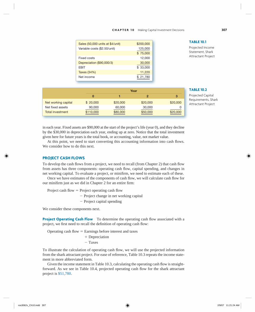
in each year. Fixed assets are $90,000 at the start of the project’s life (year 0), and they decline by the $30,000 in depreciation each year, ending up at zero. Notice that the total investment given here for future years is the total book, or accounting, value, not market value. At this point, we need to start converting this accounting information into cash fl ows. We consider how to do this next.
PROJECT CASH FLOWSTo develop the cash fl ows from a project, we need to recall (from Chapter 2) that cash fl ow from assets has three components: operating cash fl ow, capital spending, and changes in net working capital. To evaluate a project, or minifi rm, we need to estimate each of these. Once we have estimates of the components of cash fl ow, we will calculate cash fl ow for our minifi rm just as we did in Chapter 2 for an entire fi rm:
Project cash fl ow � Project operating cash fl ow
� Project change in net working capital
� Project capital spending
We consider these components next.
Project Operating Cash Flow To determine the operating cash fl ow associated with a project, we fi rst need to recall the defi nition of operating cash fl ow:
Operating cash fl ow � Earnings before interest and taxes
� Depreciation
� Taxes
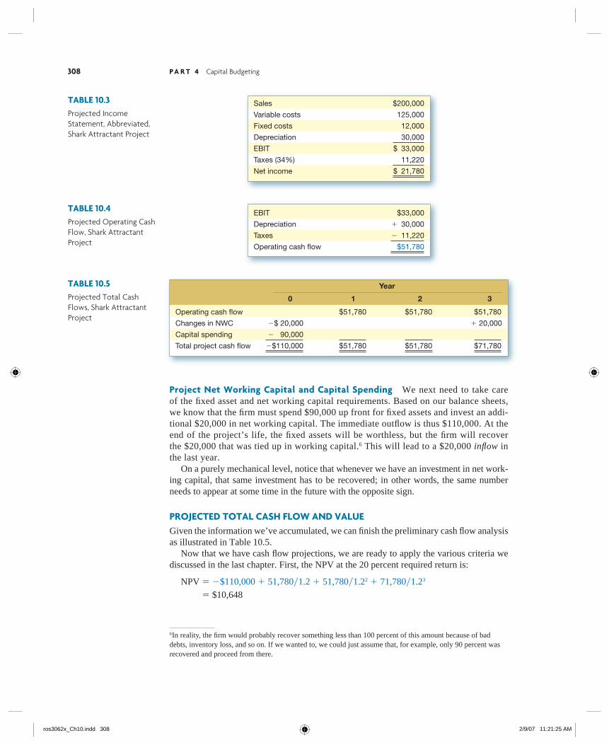
To illustrate the calculation of operating cash fl ow, we will use the projected information from the shark attractant project. For ease of reference, Table 10.3 repeats the income state-ment in more abbreviated form. Given the income statement in Table 10.3, calculating the operating cash fl ow is straight-forward. As we see in Table 10.4, projected operating cash fl ow for the shark attractant project is $51,780.
TABLE 10.1Projected Income Statement, Shark Attractant Project
Sales (50,000 units at $4/unit) $200,000
Variable costs ($2.50/unit) 125,000
$ 75,000
Fixed costs 12,000
Depreciation ($90,000�3) 30,000
EBIT $ 33,000
Taxes (34%) 11,220
Net income $ 21,780
TABLE 10.2Projected Capital Requirements, Shark Attractant Project
Year
0 1 2 3
Net working capital $ 20,000 $20,000 $20,000 $20,000
Net fi xed assets 90,000 60,000 30,000 0
Total investment $110,000 $80,000 $50,000 $20,000
ros3062x_Ch10.indd 307ros3062x_Ch10.indd 307 2/9/07 11:21:24 AM2/9/07 11:21:24 AM
308 P A R T 4 Capital Budgeting
Sales $200,000
Variable costs 125,000
Fixed costs 12,000
Depreciation 30,000
EBIT $ 33,000
Taxes (34%) 11,220
Net income $ 21,780
TABLE 10.3Projected Income Statement, Abbreviated, Shark Attractant Project
TABLE 10.4Projected Operating Cash Flow, Shark Attractant Project
EBIT $33,000
Depreciation � 30,000
Taxes � 11,220
Operating cash fl ow $51,780
Project Net Working Capital and Capital Spending We next need to take care of the fi xed asset and net working capital requirements. Based on our balance sheets, we know that the fi rm must spend $90,000 up front for fi xed assets and invest an addi-tional $20,000 in net working capital. The immediate outfl ow is thus $110,000. At the end of the project’s life, the fi xed assets will be worthless, but the fi rm will recover the $20,000 that was tied up in working capital.6 This will lead to a $20,000 infl ow in the last year. On a purely mechanical level, notice that whenever we have an investment in net work-ing capital, that same investment has to be recovered; in other words, the same number needs to appear at some time in the future with the opposite sign.
PROJECTED TOTAL CASH FLOW AND VALUEGiven the information we’ve accumulated, we can fi nish the preliminary cash fl ow analysis as illustrated in Table 10.5. Now that we have cash fl ow projections, we are ready to apply the various criteria we discussed in the last chapter. First, the NPV at the 20 percent required return is:
NPV � �$110,000 � 51,780�1.2 � 51,780�1.22 � 71,780�1.23
� $10,648
6In reality, the fi rm would probably recover something less than 100 percent of this amount because of bad debts, inventory loss, and so on. If we wanted to, we could just assume that, for example, only 90 percent was recovered and proceed from there.
Year
0 1 2 3
Operating cash fl ow $51,780 $51,780 $51,780
Changes in NWC �$ 20,000 � 20,000
Capital spending � 90,000
Total project cash fl ow �$110,000 $51,780 $51,780 $71,780
TABLE 10.5Projected Total Cash Flows, Shark Attractant Project
ros3062x_Ch10.indd 308ros3062x_Ch10.indd 308 2/9/07 11:21:25 AM2/9/07 11:21:25 AM
C H A P T E R 1 0 Making Capital Investment Decisions 309
Based on these projections, the project creates over $10,000 in value and should be accepted. Also, the return on this investment obviously exceeds 20 percent (because the NPV is positive at 20 percent). After some trial and error, we fi nd that the IRR works out to be about 25.8 percent. In addition, if required, we could calculate the payback and the average accounting return, or AAR. Inspection of the cash fl ows shows that the payback on this project is just a little over two years (verify that it’s about 2.1 years).7
From the last chapter, we know that the AAR is average net income divided by average book value. The net income each year is $21,780. The average (in thousands) of the four book values (from Table 10.2) for total investment is ($110 � 80 � 50 � 20)�4 � $65. So the AAR is $21,780�65,000 � 33.51 percent.8 We’ve already seen that the return on this investment (the IRR) is about 26 percent. The fact that the AAR is larger illustrates again why the AAR cannot be meaningfully interpreted as the return on a project.
10.3a What is the defi nition of project operating cash fl ow? How does this differ from net income?
10.3b For the shark attractant project, why did we add back the firm’s net working capital investment in the fi nal year?
Concept Questions
More about Project Cash FlowIn this section, we take a closer look at some aspects of project cash fl ow. In particular, we discuss project net working capital in more detail. We then examine current tax laws regarding depreciation. Finally, we work through a more involved example of the capital investment decision.
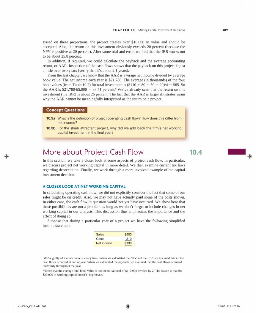
A CLOSER LOOK AT NET WORKING CAPITALIn calculating operating cash fl ow, we did not explicitly consider the fact that some of our sales might be on credit. Also, we may not have actually paid some of the costs shown. In either case, the cash fl ow in question would not yet have occurred. We show here that these possibilities are not a problem as long as we don’t forget to include changes in net working capital in our analysis. This discussion thus emphasizes the importance and the effect of doing so. Suppose that during a particular year of a project we have the following simplifi ed income statement:
Sales $500Costs 310Net income $190
10.4
7We’re guilty of a minor inconsistency here. When we calculated the NPV and the IRR, we assumed that all the cash fl ows occurred at end of year. When we calculated the payback, we assumed that the cash fl ows occurred uniformly throughout the year.8Notice that the average total book value is not the initial total of $110,000 divided by 2. The reason is that the $20,000 in working capital doesn’t “depreciate.”
ros3062x_Ch10.indd 309ros3062x_Ch10.indd 309 2/9/07 11:21:26 AM2/9/07 11:21:26 AM
310 P A R T 4 Capital Budgeting
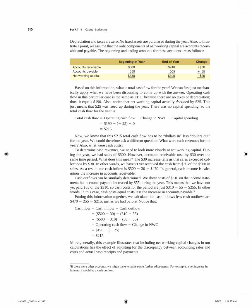
Depreciation and taxes are zero. No fi xed assets are purchased during the year. Also, to illus-trate a point, we assume that the only components of net working capital are accounts receiv-able and payable. The beginning and ending amounts for these accounts are as follows:
Beginning of Year End of Year Change
Accounts receivable $880 $910 �$30Accounts payable 550 605 � 55Net working capital $330 $305 �$25
Based on this information, what is total cash fl ow for the year? We can fi rst just mechan-ically apply what we have been discussing to come up with the answer. Operating cash fl ow in this particular case is the same as EBIT because there are no taxes or depreciation; thus, it equals $190. Also, notice that net working capital actually declined by $25. This just means that $25 was freed up during the year. There was no capital spending, so the total cash fl ow for the year is:
Total cash fl ow � Operating cash fl ow � Change in NWC � Capital spending
� $190 � (� 25) � 0
� $215
Now, we know that this $215 total cash fl ow has to be “dollars in” less “dollars out” for the year. We could therefore ask a different question: What were cash revenues for the year? Also, what were cash costs? To determine cash revenues, we need to look more closely at net working capital. Dur-ing the year, we had sales of $500. However, accounts receivable rose by $30 over the same time period. What does this mean? The $30 increase tells us that sales exceeded col-lections by $30. In other words, we haven’t yet received the cash from $30 of the $500 in sales. As a result, our cash infl ow is $500 � 30 � $470. In general, cash income is sales minus the increase in accounts receivable. Cash outfl ows can be similarly determined. We show costs of $310 on the income state-ment, but accounts payable increased by $55 during the year. This means that we have not yet paid $55 of the $310, so cash costs for the period are just $310 � 55 � $255. In other words, in this case, cash costs equal costs less the increase in accounts payable.9
Putting this information together, we calculate that cash infl ows less cash outfl ows are $470 � 255 � $215, just as we had before. Notice that:
Cash fl ow � Cash infl ow � Cash outfl ow
� ($500 � 30) � (310 � 55)
� ($500 � 310) � (30 � 55)
� Operating cash fl ow � Change in NWC
� $190 � (� 25)
� $215
More generally, this example illustrates that including net working capital changes in our calculations has the effect of adjusting for the discrepancy between accounting sales and costs and actual cash receipts and payments.
9If there were other accounts, we might have to make some further adjustments. For example, a net increase in inventory would be a cash outfl ow.
ros3062x_Ch10.indd 310ros3062x_Ch10.indd 310 2/9/07 11:21:27 AM2/9/07 11:21:27 AM
IN THEIR OWN WORDS . . .
Samuel Weaver on Capital Budgeting at The Hershey Company
The capital program at The Hershey Company and most Fortune 500 or Fortune 1,000 companies involves a three-phase approach: planning or budgeting, evaluation, and postcompletion reviews.
The fi rst phase involves identifi cation of likely projects at strategic planning time. These are selected to support the strategic objectives of the corporation. This identifi cation is generally broad in scope with minimal fi nancial evaluation attached. As the planning process focuses more closely on the short-term plans, major capital expenditures are scrutinized more rigorously. Project costs are more closely honed, and specifi c proj-ects may be reconsidered.
Each project is then individually reviewed and authorized. Planning, developing, and refi ning cash fl ows underlie capital analysis at Hershey. Once the cash fl ows have been determined, the application of capital evaluation techniques such as those using net present value, internal rate of return, and payback period is routine. Presentation of the results is enhanced using sensitivity analysis, which plays a major role for manage-ment in assessing the critical assumptions and resulting impact.
The fi nal phase relates to postcompletion reviews in which the original forecasts of the project’s performance are compared to actual results and/or revised expectations.
Capital expenditure analysis is only as good as the assumptions that underlie the project. The old cliché of GIGO (garbage in, garbage out) applies in this case. Incremental cash fl ows primarily result from incremental sales or margin improvements (cost savings). For the most part, a range of incremental cash fl ows can be identifi ed from marketing research or engineering studies. However, for a number of projects, correctly discern-ing the implications and the relevant cash fl ows is analytically challenging. For example, when a new product is introduced and is expected to generate millions of dollars’ worth of sales, the appropriate analysis focuses on the incremental sales after accounting for cannibalization of existing products.
One of the problems that we face at Hershey deals with the application of net present value, NPV, versus internal rate of return, IRR. NPV offers us the correct investment indication when dealing with mutually exclusive alternatives. However, decision makers at all levels sometimes fi nd it diffi cult to comprehend the result. Specifi -cally, an NPV of, say, $535,000 needs to be interpreted. It is not enough to know that the NPV is positive or even that it is more positive than an alternative. Decision makers seek to determine a level of “comfort” regard-ing how profi table the investment is by relating it to other standards.
Although the IRR may provide a misleading indication of which project to select, the result is provided in a way that can be interpreted by all parties. The resulting IRR can be mentally compared to expected infl ation, current borrowing rates, the cost of capital, an equity portfolio’s return, and so on. An IRR of, say, 18 percent is readily interpretable by management. Perhaps this ease of understanding is why surveys indicate that most Fortune 500 or Fortune 1,000 companies use the IRR method as a primary evaluation technique.
In addition to the NPV versus IRR problem, there are a limited number of projects for which traditional capital expenditure analysis is diffi cult to apply because the cash fl ows can’t be determined. When new computer equipment is purchased, an offi ce building is renovated, or a parking lot is repaved, it is essentially impossible to identify the cash fl ows, so the use of traditional evaluation techniques is limited. These types of “capital expendi-ture” decisions are made using other techniques that hinge on management’s judgment.
Samuel Weaver, Ph.D., is the former director, fi nancial planning and analysis, for Hershey Chocolate North America. He is a certifi ed management accountant and certifi ed fi nancial manager. His position combined the theoretical with the pragmatic and involved the analysis of many different facets of fi nance in addition to capi-tal expenditure analysis.
311
Cash Collections and Costs EXAMPLE 10.1
For the year just completed, the Combat Wombat Telestat Co. (CWT) reports sales of $998 and costs of $734. You have collected the following beginning and ending balance sheet information:
continued
ros3062x_Ch10.indd 311ros3062x_Ch10.indd 311 2/9/07 11:21:30 AM2/9/07 11:21:30 AM
312 P A R T 4 Capital Budgeting
DEPRECIATIONAs we note elsewhere, accounting depreciation is a noncash deduction. As a result, depre-ciation has cash fl ow consequences only because it infl uences the tax bill. The way that depreciation is computed for tax purposes is thus the relevant method for capital investment decisions. Not surprisingly, the procedures are governed by tax law. We now discuss some specifi cs of the depreciation system enacted by the Tax Reform Act of 1986. This system is a modifi cation of the accelerated cost recovery system (ACRS) instituted in 1981.
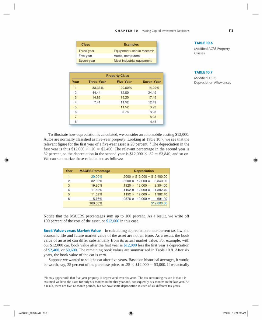
Modifi ed ACRS Depreciation (MACRS) Calculating depreciation is normally mechan-ical. Although there are a number of ifs, ands, and buts involved, the basic idea under MACRS is that every asset is assigned to a particular class. An asset’s class establishes its life for tax purposes. Once an asset’s tax life is determined, the depreciation for each year is computed by multiplying the cost of the asset by a fi xed percentage.10 The expected sal-vage value (what we think the asset will be worth when we dispose of it) and the expected economic life (how long we expect the asset to be in service) are not explicitly considered in the calculation of depreciation. Some typical depreciation classes are given in Table 10.6, and associated percentages (rounded to two decimal places) are shown in Table 10.7.11
A nonresidential real property, such as an offi ce building, is depreciated over 31.5 years using straight-line depreciation. A residential real property, such as an apartment building, is depreciated straight-line over 27.5 years. Remember that land cannot be depreciated.12
accelerated cost recovery system (ACRS)A depreciation method under U.S. tax law allowing for the accelerated write-off of property under various classifi cations.
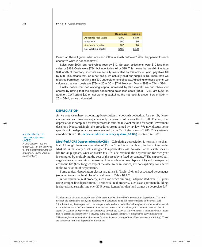
Beginning Ending
Accounts receivable $100 $110
Inventory 100 80
Accounts payable 100 70
Net working capital $100 $120
Based on these fi gures, what are cash infl ows? Cash outfl ows? What happened to each account? What is net cash fl ow? Sales were $998, but receivables rose by $10. So cash collections were $10 less than sales, or $988. Costs were $734, but inventories fell by $20. This means that we didn’t replace $20 worth of inventory, so costs are actually overstated by this amount. Also, payables fell by $30. This means that, on a net basis, we actually paid our suppliers $30 more than we received from them, resulting in a $30 understatement of costs. Adjusting for these events, we calculate that cash costs are $734 � 20 � 30 � $744. Net cash fl ow is $988 � 744 � $244. Finally, notice that net working capital increased by $20 overall. We can check our answer by noting that the original accounting sales less costs ($998 � 734) are $264. In addition, CWT spent $20 on net working capital, so the net result is a cash fl ow of $264 �
20 � $244, as we calculated.
10Under certain circumstances, the cost of the asset may be adjusted before computing depreciation. The result is called the depreciable basis, and depreciation is calculated using this number instead of the actual cost.11For the curious, these depreciation percentages are derived from a double-declining balance scheme with a switch to straight-line when the latter becomes advantageous. Further, there is a half-year convention, meaning that all assets are assumed to be placed in service midway through the tax year. This convention is maintained unless more than 40 percent of an asset’s cost is incurred in the fi nal quarter. In this case, a midquarter convention is used.12There are, however, depletion allowances for fi rms in extraction-type lines of business (such as mining). These are somewhat similar to depreciation allowances.
ros3062x_Ch10.indd 312ros3062x_Ch10.indd 312 2/9/07 11:21:32 AM2/9/07 11:21:32 AM
C H A P T E R 1 0 Making Capital Investment Decisions 313
13It may appear odd that fi ve-year property is depreciated over six years. The tax accounting reason is that it is assumed we have the asset for only six months in the fi rst year and, consequently, six months in the last year. As a result, there are fi ve 12-month periods, but we have some depreciation in each of six different tax years.
Class Examples
Three-year Equipment used in research
Five-year Autos, computers
Seven-year Most industrial equipment
Property Class
Year Three-Year Five-Year Seven-Year
1 33.33% 20.00% 14.29%
2 44.44 32.00 24.49
3 14.82 19.20 17.49
4 7.41 11.52 12.49
5 11.52 8.93
6 5.76 8.93
7 8.93
8 4.45
To illustrate how depreciation is calculated, we consider an automobile costing $12,000. Autos are normally classifi ed as fi ve-year property. Looking at Table 10.7, we see that the relevant fi gure for the fi rst year of a fi ve-year asset is 20 percent.13 The depreciation in the fi rst year is thus $12,000 � .20 � $2,400. The relevant percentage in the second year is 32 percent, so the depreciation in the second year is $12,000 � .32 � $3,840, and so on. We can summarize these calculations as follows:
Year MACRS Percentage Depreciation
1 20.00% .2000 � $12,000 � $ 2,400.00 2 32.00% .3200 � 12,000 � 3,840.00 3 19.20% .1920 � 12,000 � 2,304.00 4 11.52% .1152 � 12,000 � 1,382.40 5 11.52% .1152 � 12,000 � 1,382.40 6 5.76% .0576 � 12,000 � 691.20 100.00% $12,000.00
Notice that the MACRS percentages sum up to 100 percent. As a result, we write off 100 percent of the cost of the asset, or $12,000 in this case.
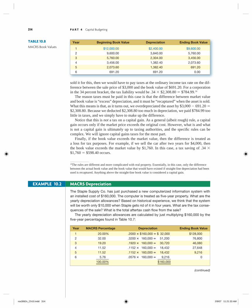
Book Value versus Market Value In calculating depreciation under current tax law, the economic life and future market value of the asset are not an issue. As a result, the book value of an asset can differ substantially from its actual market value. For example, with our $12,000 car, book value after the fi rst year is $12,000 less the fi rst year’s depreciation of $2,400, or $9,600. The remaining book values are summarized in Table 10.8. After six years, the book value of the car is zero. Suppose we wanted to sell the car after fi ve years. Based on historical averages, it would be worth, say, 25 percent of the purchase price, or .25 � $12,000 � $3,000. If we actually
TABLE 10.6Modifi ed ACRS Property Classes
TABLE 10.7Modifi ed ACRS Depreciation Allowances
ros3062x_Ch10.indd 313ros3062x_Ch10.indd 313 2/9/07 11:21:32 AM2/9/07 11:21:32 AM
314 P A R T 4 Capital Budgeting
sold it for this, then we would have to pay taxes at the ordinary income tax rate on the dif-ference between the sale price of $3,000 and the book value of $691.20. For a corporation in the 34 percent bracket, the tax liability would be .34 � $2,308.80 � $784.99.14
The reason taxes must be paid in this case is that the difference between market value and book value is “excess” depreciation, and it must be “recaptured” when the asset is sold. What this means is that, as it turns out, we overdepreciated the asset by $3,000 � 691.20 � $2,308.80. Because we deducted $2,308.80 too much in depreciation, we paid $784.99 too little in taxes, and we simply have to make up the difference. Notice that this is not a tax on a capital gain. As a general (albeit rough) rule, a capital gain occurs only if the market price exceeds the original cost. However, what is and what is not a capital gain is ultimately up to taxing authorities, and the specifi c rules can be complex. We will ignore capital gains taxes for the most part. Finally, if the book value exceeds the market value, then the difference is treated as a loss for tax purposes. For example, if we sell the car after two years for $4,000, then the book value exceeds the market value by $1,760. In this case, a tax saving of .34 � $1,760 � $598.40 occurs.
14The rules are different and more complicated with real property. Essentially, in this case, only the difference between the actual book value and the book value that would have existed if straight-line depreciation had been used is recaptured. Anything above the straight-line book value is considered a capital gain.
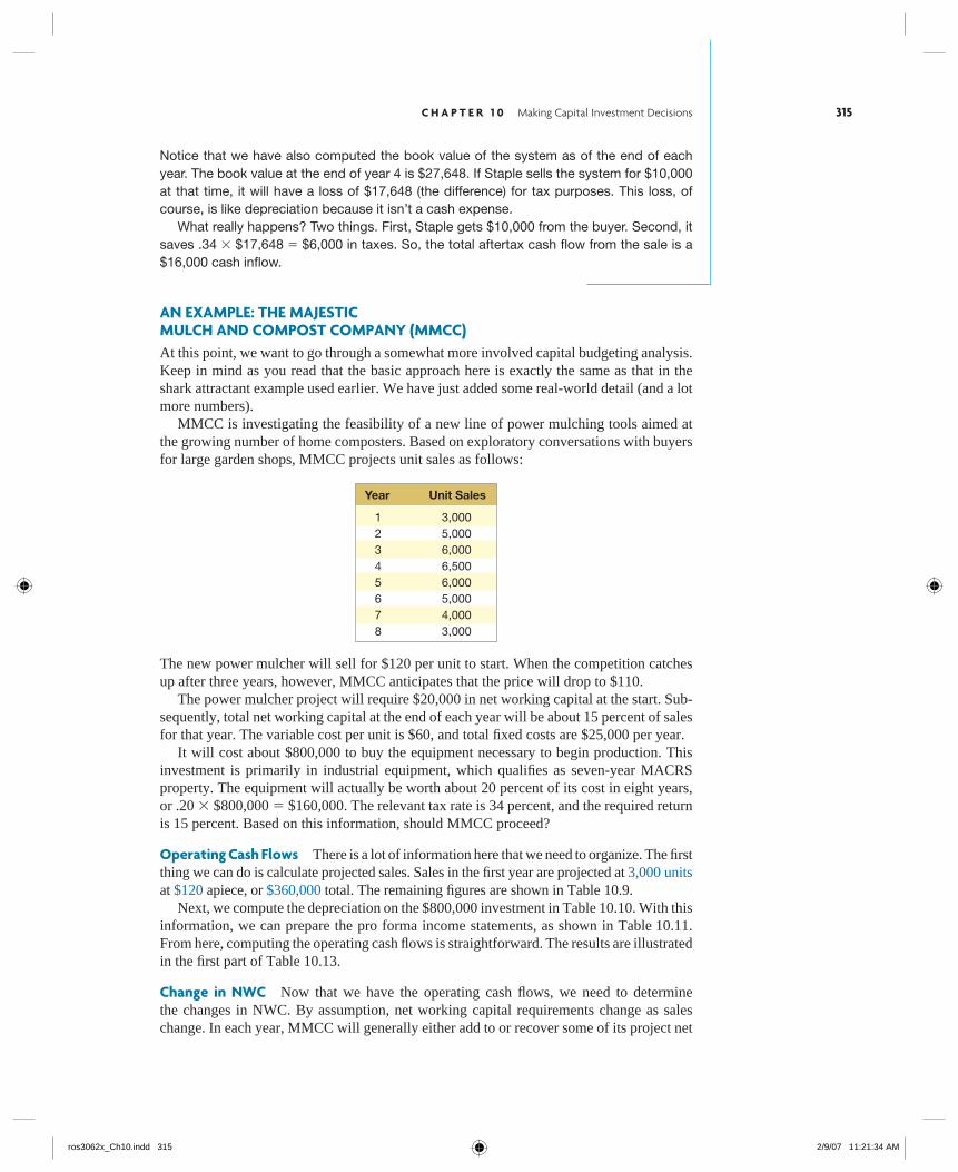
The Staple Supply Co. has just purchased a new computerized information system with an installed cost of $160,000. The computer is treated as fi ve-year property. What are the yearly depreciation allowances? Based on historical experience, we think that the system will be worth only $10,000 when Staple gets rid of it in four years. What are the tax conse-quences of the sale? What is the total aftertax cash fl ow from the sale? The yearly depreciation allowances are calculated by just multiplying $160,000 by the fi ve-year percentages found in Table 10.7:
Year MACRS Percentage Depreciation Ending Book Value
1 20.00% .2000 � $160,000 � $ 32,000 $128,000
2 32.00 .3200 � 160,000 � 51,200 76,800
3 19.20 .1920 � 160,000 � 30,720 46,080
4 11.52 .1152 � 160,000 � 18,432 27,648
5 11.52 .1152 � 160,000 � 18,432 9,216
6 5.76 .0576 � 160,000 � 9,216 0
100.00% $160,000
(continued)
EXAMPLE 10.2 MACRS Depreciation
TABLE 10.8MACRS Book Values
Year Beginning Book Value Depreciation Ending Book Value
1 $12,000.00 $2,400.00 $9,600.00
2 9,600.00 3,840.00 5,760.00
3 5,760.00 2,304.00 3,456.00
4 3,456.00 1,382.40 2,073.60
5 2,073.60 1,382.40 691.20
6 691.20 691.20 0.00
ros3062x_Ch10.indd 314ros3062x_Ch10.indd 314 2/9/07 11:21:33 AM2/9/07 11:21:33 AM
C H A P T E R 1 0 Making Capital Investment Decisions 315
Notice that we have also computed the book value of the system as of the end of each year. The book value at the end of year 4 is $27,648. If Staple sells the system for $10,000 at that time, it will have a loss of $17,648 (the difference) for tax purposes. This loss, of course, is like depreciation because it isn’t a cash expense. What really happens? Two things. First, Staple gets $10,000 from the buyer. Second, it saves .34 � $17,648 � $6,000 in taxes. So, the total aftertax cash fl ow from the sale is a $16,000 cash infl ow.
AN EXAMPLE: THE MAJESTIC MULCH AND COMPOST COMPANY (MMCC)At this point, we want to go through a somewhat more involved capital budgeting analysis. Keep in mind as you read that the basic approach here is exactly the same as that in the shark attractant example used earlier. We have just added some real-world detail (and a lot more numbers). MMCC is investigating the feasibility of a new line of power mulching tools aimed at the growing number of home composters. Based on exploratory conversations with buyers for large garden shops, MMCC projects unit sales as follows:
Year Unit Sales
1 3,000 2 5,000 3 6,000 4 6,500 5 6,000 6 5,000 7 4,000 8 3,000
The new power mulcher will sell for $120 per unit to start. When the competition catches up after three years, however, MMCC anticipates that the price will drop to $110. The power mulcher project will require $20,000 in net working capital at the start. Sub-sequently, total net working capital at the end of each year will be about 15 percent of sales for that year. The variable cost per unit is $60, and total fi xed costs are $25,000 per year. It will cost about $800,000 to buy the equipment necessary to begin production. This investment is primarily in industrial equipment, which qualifi es as seven-year MACRS property. The equipment will actually be worth about 20 percent of its cost in eight years, or .20 � $800,000 � $160,000. The relevant tax rate is 34 percent, and the required return is 15 percent. Based on this information, should MMCC proceed?
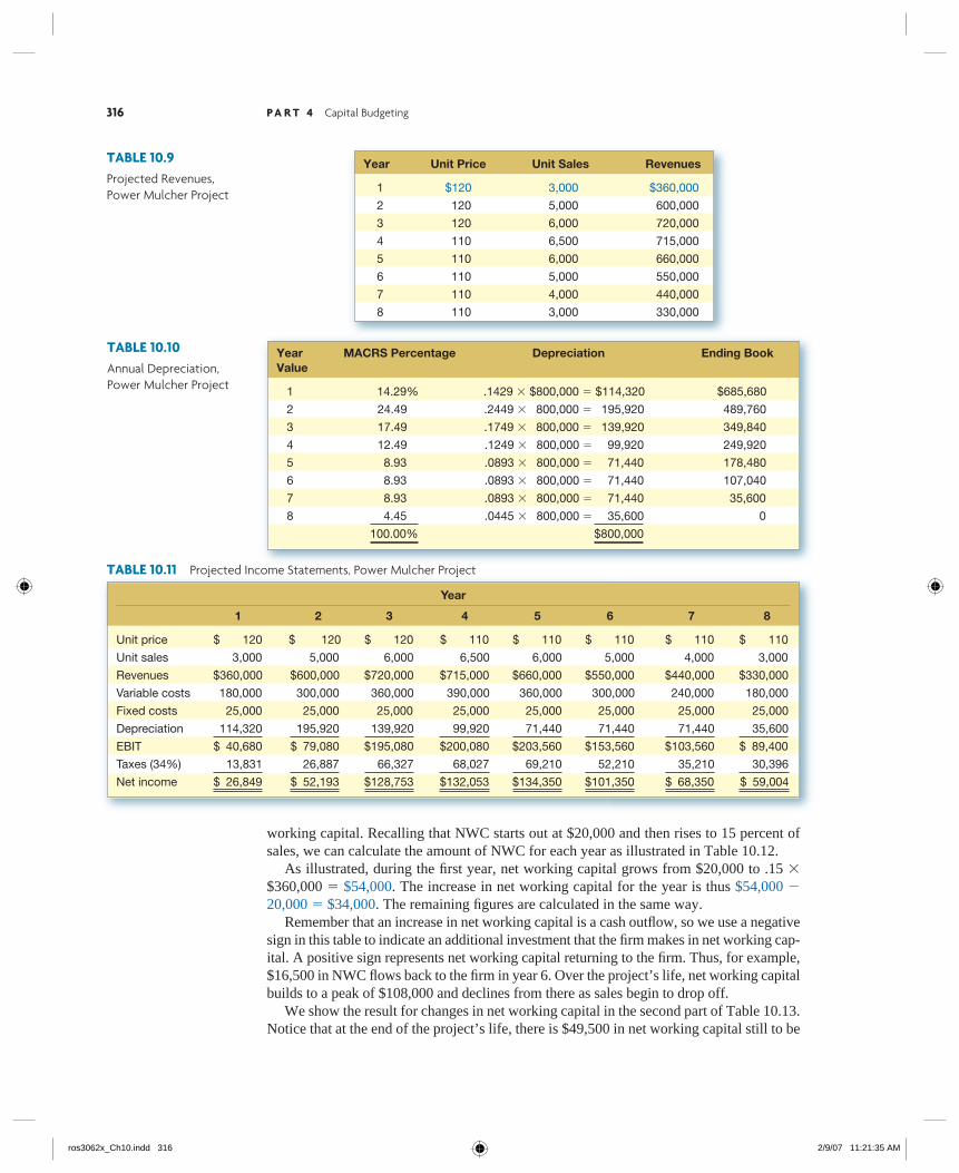
Operating Cash Flows There is a lot of information here that we need to organize. The fi rst thing we can do is calculate projected sales. Sales in the fi rst year are projected at 3,000 units at $120 apiece, or $360,000 total. The remaining fi gures are shown in Table 10.9. Next, we compute the depreciation on the $800,000 investment in Table 10.10. With this information, we can prepare the pro forma income statements, as shown in Table 10.11. From here, computing the operating cash fl ows is straightforward. The results are illustrated in the fi rst part of Table 10.13.
Change in NWC Now that we have the operating cash fl ows, we need to determine the changes in NWC. By assumption, net working capital requirements change as sales change. In each year, MMCC will generally either add to or recover some of its project net
ros3062x_Ch10.indd 315ros3062x_Ch10.indd 315 2/9/07 11:21:34 AM2/9/07 11:21:34 AM
316 P A R T 4 Capital Budgeting
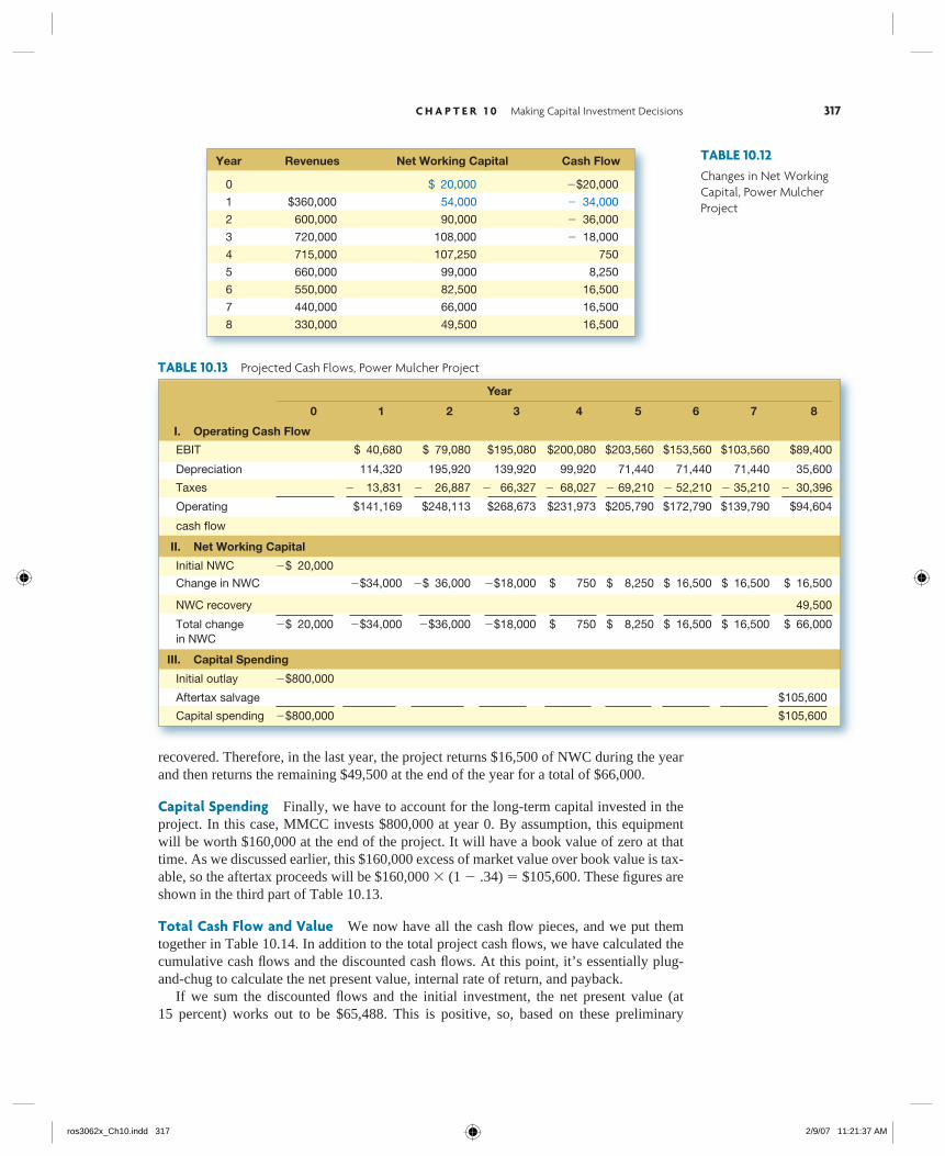
working capital. Recalling that NWC starts out at $20,000 and then rises to 15 percent of sales, we can calculate the amount of NWC for each year as illustrated in Table 10.12. As illustrated, during the fi rst year, net working capital grows from $20,000 to .15 � $360,000 � $54,000. The increase in net working capital for the year is thus $54,000 � 20,000 � $34,000. The remaining fi gures are calculated in the same way. Remember that an increase in net working capital is a cash outfl ow, so we use a negative sign in this table to indicate an additional investment that the fi rm makes in net working cap-ital. A positive sign represents net working capital returning to the fi rm. Thus, for example, $16,500 in NWC fl ows back to the fi rm in year 6. Over the project’s life, net working capital builds to a peak of $108,000 and declines from there as sales begin to drop off. We show the result for changes in net working capital in the second part of Table 10.13. Notice that at the end of the project’s life, there is $49,500 in net working capital still to be
TABLE 10.9Projected Revenues, Power Mulcher Project
Year Unit Price Unit Sales Revenues
1 $120 3,000 $360,000
2 120 5,000 600,000
3 120 6,000 720,000
4 110 6,500 715,000
5 110 6,000 660,000
6 110 5,000 550,000
7 110 4,000 440,000
8 110 3,000 330,000
TABLE 10.10Annual Depreciation, Power Mulcher Project
Year MACRS Percentage Depreciation Ending Book Value
1 14.29% .1429 � $800,000 � $114,320 $685,680
2 24.49 .2449 � 800,000 � 195,920 489,760
3 17.49 .1749 � 800,000 � 139,920 349,840
4 12.49 .1249 � 800,000 � 99,920 249,920
5 8.93 .0893 � 800,000 � 71,440 178,480
6 8.93 .0893 � 800,000 � 71,440 107,040
7 8.93 .0893 � 800,000 � 71,440 35,600
8 4.45 .0445 � 800,000 � 35,600 0
100.00% $800,000
TABLE 10.11 Projected Income Statements, Power Mulcher Project
Year
1 2 3 4 5 6 7 8
Unit price $ 120 $ 120 $ 120 $ 110 $ 110 $ 110 $ 110 $ 110
Unit sales 3,000 5,000 6,000 6,500 6,000 5,000 4,000 3,000
Revenues $360,000 $600,000 $720,000 $715,000 $660,000 $550,000 $440,000 $330,000
Variable costs 180,000 300,000 360,000 390,000 360,000 300,000 240,000 180,000
Fixed costs 25,000 25,000 25,000 25,000 25,000 25,000 25,000 25,000
Depreciation 114,320 195,920 139,920 99,920 71,440 71,440 71,440 35,600
EBIT $ 40,680 $ 79,080 $195,080 $200,080 $203,560 $153,560 $103,560 $ 89,400
Taxes (34%) 13,831 26,887 66,327 68,027 69,210 52,210 35,210 30,396
Net income $ 26,849 $ 52,193 $128,753 $132,053 $134,350 $101,350 $ 68,350 $ 59,004
ros3062x_Ch10.indd 316ros3062x_Ch10.indd 316 2/9/07 11:21:35 AM2/9/07 11:21:35 AM
C H A P T E R 1 0 Making Capital Investment Decisions 317
recovered. Therefore, in the last year, the project returns $16,500 of NWC during the year and then returns the remaining $49,500 at the end of the year for a total of $66,000.
Capital Spending Finally, we have to account for the long-term capital invested in the project. In this case, MMCC invests $800,000 at year 0. By assumption, this equipment will be worth $160,000 at the end of the project. It will have a book value of zero at that time. As we discussed earlier, this $160,000 excess of market value over book value is tax-able, so the aftertax proceeds will be $160,000 � (1 � .34) � $105,600. These fi gures are shown in the third part of Table 10.13.
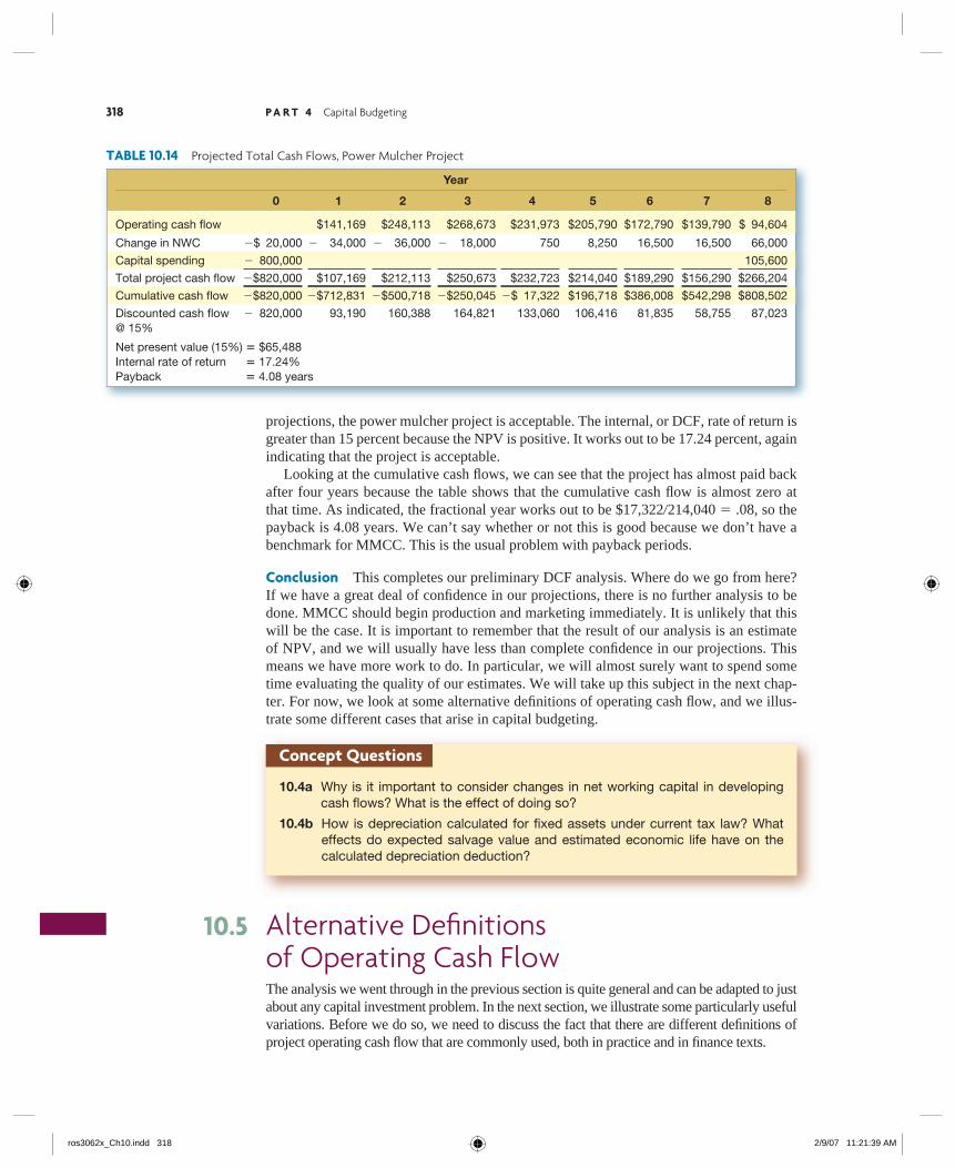
Total Cash Flow and Value We now have all the cash fl ow pieces, and we put them together in Table 10.14. In addition to the total project cash fl ows, we have calculated the cumulative cash fl ows and the discounted cash fl ows. At this point, it’s essentially plug-and-chug to calculate the net present value, internal rate of return, and payback. If we sum the discounted fl ows and the initial investment, the net present value (at 15 percent) works out to be $65,488. This is positive, so, based on these preliminary
Year
0 1 2 3 4 5 6 7 8
I. Operating Cash Flow
EBIT $ 40,680 $ 79,080 $195,080 $200,080 $203,560 $153,560 $103,560 $89,400
Depreciation 114,320 195,920 139,920 99,920 71,440 71,440 71,440 35,600
Taxes � 13,831 � 26,887 � 66,327 � 68,027 � 69,210 � 52,210 � 35,210 � 30,396
Operating $141,169 $248,113 $268,673 $231,973 $205,790 $172,790 $139,790 $94,604
cash fl ow
II. Net Working Capital
Initial NWC �$ 20,000
Change in NWC �$34,000 �$ 36,000 �$18,000 $ 750 $ 8,250 $ 16,500 $ 16,500 $ 16,500
NWC recovery 49,500
Total change in NWC
�$ 20,000 �$34,000 �$36,000 �$18,000 $ 750 $ 8,250 $ 16,500 $ 16,500 $ 66,000
III. Capital Spending
Initial outlay �$800,000
Aftertax salvage $105,600
Capital spending �$800,000 $105,600
TABLE 10.13 Projected Cash Flows, Power Mulcher Project
TABLE 10.12Changes in Net Working Capital, Power Mulcher Project
Year Revenues Net Working Capital Cash Flow
0 $ 20,000 �$20,000
1 $360,000 54,000 � 34,000
2 600,000 90,000 � 36,000
3 720,000 108,000 � 18,000
4 715,000 107,250 750
5 660,000 99,000 8,250
6 550,000 82,500 16,500
7 440,000 66,000 16,500
8 330,000 49,500 16,500
ros3062x_Ch10.indd 317ros3062x_Ch10.indd 317 2/9/07 11:21:37 AM2/9/07 11:21:37 AM
318 P A R T 4 Capital Budgeting
projections, the power mulcher project is acceptable. The internal, or DCF, rate of return is greater than 15 percent because the NPV is positive. It works out to be 17.24 percent, again indicating that the project is acceptable. Looking at the cumulative cash fl ows, we can see that the project has almost paid back after four years because the table shows that the cumulative cash fl ow is almost zero at that time. As indicated, the fractional year works out to be $17,322�214,040 � .08, so the payback is 4.08 years. We can’t say whether or not this is good because we don’t have a benchmark for MMCC. This is the usual problem with payback periods.
Conclusion This completes our preliminary DCF analysis. Where do we go from here? If we have a great deal of confi dence in our projections, there is no further analysis to be done. MMCC should begin production and marketing immediately. It is unlikely that this will be the case. It is important to remember that the result of our analysis is an estimate of NPV, and we will usually have less than complete confi dence in our projections. This means we have more work to do. In particular, we will almost surely want to spend some time evaluating the quality of our estimates. We will take up this subject in the next chap-ter. For now, we look at some alternative defi nitions of operating cash fl ow, and we illus-trate some different cases that arise in capital budgeting.
10.4a Why is it important to consider changes in net working capital in developing cash fl ows? What is the effect of doing so?
10.4b How is depreciation calculated for fixed assets under current tax law? What effects do expected salvage value and estimated economic life have on the calculated depreciation deduction?
Concept Questions
Alternative Defi nitions of Operating Cash FlowThe analysis we went through in the previous section is quite general and can be adapted to just about any capital investment problem. In the next section, we illustrate some particularly useful variations. Before we do so, we need to discuss the fact that there are different defi nitions of project operating cash fl ow that are commonly used, both in practice and in fi nance texts.
10.5
Year
0 1 2 3 4 5 6 7 8
Operating cash fl ow $141,169 $248,113 $268,673 $231,973 $205,790 $172,790 $139,790 $ 94,604
Change in NWC �$ 20,000 � 34,000 � 36,000 � 18,000 750 8,250 16,500 16,500 66,000
Capital spending � 800,000 105,600
Total project cash fl ow �$820,000 $107,169 $212,113 $250,673 $232,723 $214,040 $189,290 $156,290 $266,204
Cumulative cash fl ow �$820,000 �$712,831 �$500,718 �$250,045 �$ 17,322 $196,718 $386,008 $542,298 $808,502
Discounted cash fl ow@ 15%
� 820,000 93,190 160,388 164,821 133,060 106,416 81,835 58,755 87,023
Net present value (15%) � $65,488Internal rate of return � 17.24%Payback � 4.08 years
TABLE 10.14 Projected Total Cash Flows, Power Mulcher Project
ros3062x_Ch10.indd 318ros3062x_Ch10.indd 318 2/9/07 11:21:39 AM2/9/07 11:21:39 AM
C H A P T E R 1 0 Making Capital Investment Decisions 319
As we will see, the different approaches to operating cash fl ow that exist all measure the same thing. If they are used correctly, they all produce the same answer, and one is not necessarily any better or more useful than another. Unfortunately, the fact that alternative defi nitions are used does sometimes lead to confusion. For this reason, we examine several of these variations next to see how they are related. In the discussion that follows, keep in mind that when we speak of cash fl ow, we liter-ally mean dollars in less dollars out. This is all we are concerned with. Different defi nitions of operating cash fl ow simply amount to different ways of manipulating basic information about sales, costs, depreciation, and taxes to get at cash fl ow. For a particular project and year under consideration, suppose we have the following estimates:
Sales � $1,500
Costs � $700
Depreciation � $600
With these estimates, notice that EBIT is:
EBIT � Sales � Costs � Depreciation
� $1,500 � 700 � 600
� $200
Once again, we assume that no interest is paid, so the tax bill is:
Taxes � EBIT � T
� $200 � .34 � $68
where T, the corporate tax rate, is 34 percent. When we put all of this together, we see that project operating cash fl ow, OCF, is:
OCF � EBIT � Depreciation � Taxes
� $200 � 600 � 68 � $732
There are some other ways to determine OCF that could be (and are) used. We consider these next.
THE BOTTOM-UP APPROACHBecause we are ignoring any fi nancing expenses, such as interest, in our calculations of project OCF, we can write project net income as:
Project net income � EBIT � Taxes
� $200 � 68
� $132
If we simply add the depreciation to both sides, we arrive at a slightly different and very common expression for OCF:
OCF � Net income � Depreciation
� $132 � 600 [10.1]
� $732
This is the bottom-up approach. Here, we start with the accountant’s bottom line (net income) and add back any noncash deductions such as depreciation. It is crucial to remem-ber that this defi nition of operating cash fl ow as net income plus depreciation is correct only if there is no interest expense subtracted in the calculation of net income.
ros3062x_Ch10.indd 319ros3062x_Ch10.indd 319 2/9/07 11:21:41 AM2/9/07 11:21:41 AM
320 P A R T 4 Capital Budgeting
For the shark attractant project, net income was $21,780 and depreciation was $30,000, so the bottom-up calculation is:
OCF � $21,780 � 30,000 � $51,780
This is exactly the same OCF we had previously.
THE TOP-DOWN APPROACHPerhaps the most obvious way to calculate OCF is:
OCF � Sales � Costs � Taxes
� $1,500 � 700 � 68 � $732 [10.2]
This is the top-down approach, the second variation on the basic OCF defi nition. Here, we start at the top of the income statement with sales and work our way down to net cash fl ow by subtracting costs, taxes, and other expenses. Along the way, we simply leave out any strictly noncash items such as depreciation. For the shark attractant project, the operating cash fl ow can be readily calculated using the top-down approach. With sales of $200,000, total costs (fi xed plus variable) of $137,000, and a tax bill of $11,220, the OCF is:
OCF � $200,000 � 137,000 � 11,220 � $51,780
This is just as we had before.
THE TAX SHIELD APPROACHThe third variation on our basic defi nition of OCF is the tax shield approach. This approach will be useful for some problems we consider in the next section. The tax shield defi nition of OCF is:
OCF � (Sales � Costs) � (1 � T ) � Depreciation � T [10.3]
where T is again the corporate tax rate. Assuming that T � 34%, the OCF works out to be:
OCF � ($1,500 � 700) � .66 � 600 � .34
� $528 � 204
� $732
This is just as we had before. This approach views OCF as having two components. The fi rst part is what the proj ect’s cash fl ow would be if there were no depreciation expense. In this case, this would-have-been cash fl ow is $528. The second part of OCF in this approach is the depreciation deduction multiplied by the tax rate. This is called the depreciation tax shield. We know that depreciation is a noncash expense. The only cash fl ow effect of deducting depreciation is to reduce our taxes, a ben-efi t to us. At the current 34 percent corporate tax rate, every dollar in depreciation expense saves us 34 cents in taxes. So, in our example, the $600 depreciation deduction saves us $600 � .34 � $204 in taxes. For the shark attractant project we considered earlier in the chapter, the depreciation tax -shield would be $30,000 � .34 � $10,200. The aftertax value for sales less costs would be ($200,000 � 137,000) � (1 � .34) � $41,580. Adding these together yields the value of OCF:
OCF � $41,580 � 10,200 � $51,780
This calculation verifi es that the tax shield approach is completely equivalent to the approach we used before.
depreciation tax shieldThe tax saving that results from the depreciation deduction, calculated as depreciation multiplied by the corporate tax rate.
ros3062x_Ch10.indd 320ros3062x_Ch10.indd 320 2/9/07 11:21:41 AM2/9/07 11:21:41 AM
C H A P T E R 1 0 Making Capital Investment Decisions 321
CONCLUSIONNow that we’ve seen that all of these approaches are the same, you’re probably wondering why everybody doesn’t just agree on one of them. One reason, as we will see in the next section, is that different approaches are useful in different circumstances. The best one to use is whichever happens to be the most convenient for the problem at hand.
10.5a What are the top-down and bottom-up defi nitions of operating cash fl ow?
10.5b What is meant by the term depreciation tax shield?
Concept Questions
Some Special Cases of Discounted Cash Flow AnalysisTo fi nish our chapter, we look at three common cases involving discounted cash fl ow anal-ysis. The fi rst case involves investments that are primarily aimed at improving effi ciency and thereby cutting costs. The second case we consider comes up when a fi rm is involved in submitting competitive bids. The third and fi nal case arises in choosing between equip-ment options with different economic lives.
We could consider many other special cases, but these three are particularly important because problems similar to these are so common. Also, they illustrate some diverse appli-cations of cash fl ow analysis and DCF valuation.
EVALUATING COST-CUTTING PROPOSALSOne decision we frequently face is whether to upgrade existing facilities to make them more cost-effective. The issue is whether the cost savings are large enough to justify the necessary capital expenditure. For example, suppose we are considering automating some part of an existing pro-duction process. The necessary equipment costs $80,000 to buy and install. The automa-tion will save $22,000 per year (before taxes) by reducing labor and material costs. For simplicity, assume that the equipment has a fi ve-year life and is depreciated to zero on a straight-line basis over that period. It will actually be worth $20,000 in fi ve years. Should we automate? The tax rate is 34 percent, and the discount rate is 10 percent. As always, the fi rst step in making such a decision is to identify the relevant incremental cash fl ows. First, determining the relevant capital spending is easy enough. The initial cost is $80,000. The aftertax salvage value is $20,000 � (1 � .34) � $13,200 because the book value will be zero in fi ve years. Second, there are no working capital consequences here, so we don’t need to worry about changes in net working capital. Operating cash fl ows are the third component to consider. Buying the new equipment affects our operating cash fl ows in two ways. First, we save $22,000 before taxes every year. In other words, the fi rm’s operating income increases by $22,000, so this is the relevant incremental project operating income. Second (and it’s easy to overlook this), we have an additional depreciation deduction. In this case, the depreciation is $80,000�5 � $16,000 per year. Because the project has an operating income of $22,000 (the annual pretax cost saving) and a depreciation deduction of $16,000, taking the project will increase the fi rm’s EBIT by $22,000 � 16,000 � $6,000, so this is the project’s EBIT.
10.6
ros3062x_Ch10.indd 321ros3062x_Ch10.indd 321 2/9/07 11:21:42 AM2/9/07 11:21:42 AM
322 P A R T 4 Capital Budgeting
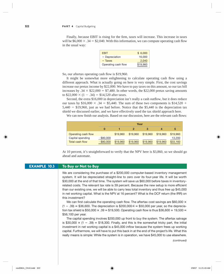
Finally, because EBIT is rising for the fi rm, taxes will increase. This increase in taxes will be $6,000 � .34 � $2,040. With this information, we can compute operating cash fl ow in the usual way:
EBIT $ 6,000� Depreciation 16,000� Taxes 2,040Operating cash fl ow $19,960
So, our aftertax operating cash fl ow is $19,960. It might be somewhat more enlightening to calculate operating cash fl ow using a different approach. What is actually going on here is very simple. First, the cost savings increase our pretax income by $22,000. We have to pay taxes on this amount, so our tax bill increases by .34 � $22,000 � $7,480. In other words, the $22,000 pretax saving amounts to $22,000 � (1 � .34) � $14,520 after taxes. Second, the extra $16,000 in depreciation isn’t really a cash outfl ow, but it does reduce our taxes by $16,000 � .34 � $5,440. The sum of these two components is $14,520 � 5,440 � $19,960, just as we had before. Notice that the $5,440 is the depreciation tax shield we discussed earlier, and we have effectively used the tax shield approach here. We can now fi nish our analysis. Based on our discussion, here are the relevant cash fl ows:
Year
0 1 2 3 4 5
Operating cash fl ow $19,960 $19,960 $19,960 $19,960 $19,960Capital spending �$80,000 13,200Total cash fl ow �$80,000 $19,960 $19,960 $19,960 $19,960 $33,160
At 10 percent, it’s straightforward to verify that the NPV here is $3,860, so we should go ahead and automate.
We are considering the purchase of a $200,000 computer-based inventory management system. It will be depreciated straight-line to zero over its four-year life. It will be worth $30,000 at the end of that time. The system will save us $60,000 before taxes in inventory-related costs. The relevant tax rate is 39 percent. Because the new setup is more effi cient than our existing one, we will be able to carry less total inventory and thus free up $45,000 in net working capital. What is the NPV at 16 percent? What is the DCF return (the IRR) on this investment? We can fi rst calculate the operating cash fl ow. The aftertax cost savings are $60,000 �
(1 � .39) � $36,600. The depreciation is $200,000�4 � $50,000 per year, so the deprecia-tion tax shield is $50,000 � .39 � $19,500. Operating cash fl ow is thus $36,600 � 19,500 �
$56,100 per year. The capital spending involves $200,000 up front to buy the system. The aftertax salvage is $30,000 � (1 � .39) � $18,300. Finally, and this is the somewhat tricky part, the initial investment in net working capital is a $45,000 infl ow because the system frees up working capital. Furthermore, we will have to put this back in at the end of the project’s life. What this really means is simple: While the system is in operation, we have $45,000 to use elsewhere.
(continued)
EXAMPLE 10.3 To Buy or Not to Buy
ros3062x_Ch10.indd 322ros3062x_Ch10.indd 322 2/9/07 11:21:43 AM2/9/07 11:21:43 AM
C H A P T E R 1 0 Making Capital Investment Decisions 323
SETTING THE BID PRICEEarly on, we used discounted cash fl ow analysis to evaluate a proposed new product. A somewhat different (and common) scenario arises when we must submit a competitive bid to win a job. Under such circumstances, the winner is whoever submits the lowest bid. There is an old joke concerning this process: The low bidder is whoever makes the big-gest mistake. This is called the winner’s curse. In other words, if you win, there is a good chance you underbid. In this section, we look at how to go about setting the bid price to avoid the winner’s curse. The procedure we describe is useful any time we have to set a price on a product or service. As with any other capital budgeting project, we must be careful to account for all relevant cash fl ows. For example, industry analysts estimated that the materials in Microsoft’s Xbox 360 cost $470 before assembly. Other items such as the power supply, cables, and controllers increased the material cost by another $55. At a retail price of $399, Microsoft obviously loses a signifi cant amount on each Xbox 360 it sells. Why would a manufacturer sell at a price well below breakeven? A Microsoft spokesperson stated that the company believed that sales of its game software would make the Xbox 360 a profi table project. To illustrate how to go about setting a bid price, imagine we are in the business of buy-ing stripped-down truck platforms and then modifying them to customer specifi cations for resale. A local distributor has requested bids for 5 specially modifi ed trucks each year for the next four years, for a total of 20 trucks in all. We need to decide what price per truck to bid. The goal of our analysis is to determine the lowest price we can profi tably charge. This maximizes our chances of being awarded the contract while guarding against the winner’s curse. Suppose we can buy the truck platforms for $10,000 each. The facilities we need can be leased for $24,000 per year. The labor and material cost to do the modifi cation works out to be about $4,000 per truck. Total cost per year will thus be $24,000 � 5 � (10,000 � 4,000) � $94,000. We will need to invest $60,000 in new equipment. This equipment will be depreciated straight-line to a zero salvage value over the four years. It will be worth about $5,000 at the end of that time. We will also need to invest $40,000 in raw materials inventory and other working capital items. The relevant tax rate is 39 percent. What price per truck should we bid if we require a 20 percent return on our investment? We start by looking at the capital spending and net working capital investment. We have to spend $60,000 today for new equipment. The aftertax salvage value is $5,000 � (1 � .39) � $3,050. Furthermore, we have to invest $40,000 today in working capital. We will get this back in four years.
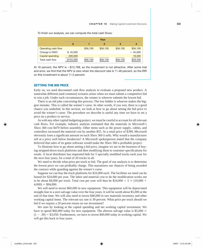
To fi nish our analysis, we can compute the total cash fl ows:
Year
0 1 2 3 4
Operating cash fl ow $56,100 $56,100 $56,100 $56,100
Change in NWC $ 45,000 � 45,000
Capital spending � 200,000 18,300
Total cash fl ow �$155,000 $56,100 $56,100 $56,100 $29,400
At 16 percent, the NPV is �$12,768, so the investment is not attractive. After some trial and error, we fi nd that the NPV is zero when the discount rate is 11.48 percent, so the IRR on this investment is about 11.5 percent.
ros3062x_Ch10.indd 323ros3062x_Ch10.indd 323 2/9/07 11:21:43 AM2/9/07 11:21:43 AM
324 P A R T 4 Capital Budgeting
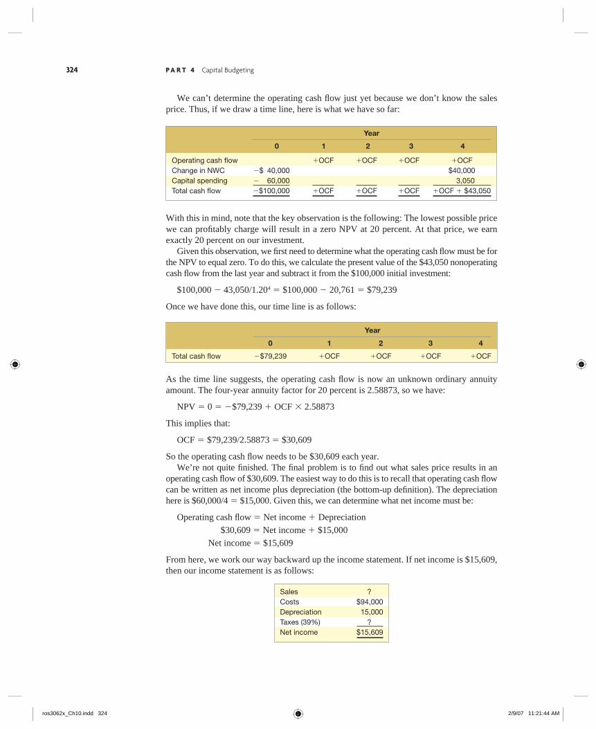
We can’t determine the operating cash fl ow just yet because we don’t know the sales price. Thus, if we draw a time line, here is what we have so far:
Year
0 1 2 3 4
Operating cash fl ow �OCF �OCF �OCF �OCFChange in NWC �$ 40,000 $40,000Capital spending � 60,000 3,050Total cash fl ow �$100,000 �OCF �OCF �OCF �OCF � $43,050
With this in mind, note that the key observation is the following: The lowest possible price we can profi tably charge will result in a zero NPV at 20 percent. At that price, we earn exactly 20 percent on our investment. Given this observation, we fi rst need to determine what the operating cash fl ow must be for the NPV to equal zero. To do this, we calculate the present value of the $43,050 nonoperating cash fl ow from the last year and subtract it from the $100,000 initial investment:
$100,000 � 43,050�1.204 � $100,000 � 20,761 � $79,239
Once we have done this, our time line is as follows:
Year
0 1 2 3 4
Total cash fl ow �$79,239 �OCF �OCF �OCF �OCF
As the time line suggests, the operating cash fl ow is now an unknown ordinary annuity amount. The four-year annuity factor for 20 percent is 2.58873, so we have:
NPV � 0 � �$79,239 � OCF � 2.58873
This implies that:
OCF � $79,239�2.58873 � $30,609
So the operating cash fl ow needs to be $30,609 each year. We’re not quite fi nished. The fi nal problem is to fi nd out what sales price results in an operating cash fl ow of $30,609. The easiest way to do this is to recall that operating cash fl ow can be written as net income plus depreciation (the bottom-up defi nition). The depreciation here is $60,000�4 � $15,000. Given this, we can determine what net income must be:
Operating cash fl ow � Net income � Depreciation
$30,609 � Net income � $15,000
Net income � $15,609
From here, we work our way backward up the income statement. If net income is $15,609, then our income statement is as follows:
Sales ?Costs $94,000Depreciation 15,000Taxes (39%) ?Net income $15,609
ros3062x_Ch10.indd 324ros3062x_Ch10.indd 324 2/9/07 11:21:44 AM2/9/07 11:21:44 AM
C H A P T E R 1 0 Making Capital Investment Decisions 325
So we can solve for sales by noting that:
Net income � (Sales � Costs � Depreciation) � (1 � T ) $15,609 � (Sales � $94,000 � $15,000) � (1 � .39) Sales � $15,609�.61 � 94,000 � 15,000 � $134,589
Sales per year must be $134,589. Because the contract calls for fi ve trucks per year, the sales price has to be $134,589�5 � $26,918. If we round this up a bit, it looks as though we need to bid about $27,000 per truck. At this price, were we to get the contract, our return would be just over 20 percent.
EVALUATING EQUIPMENT OPTIONS WITH DIFFERENT LIVESThe fi nal problem we consider involves choosing among different possible systems, equipment setups, or procedures. Our goal is to choose the most cost-effective. The approach we con-sider here is necessary only when two special circumstances exist. First, the possibilities under evaluation have different economic lives. Second, and just as important, we will need whatever we buy more or less indefi nitely. As a result, when it wears out, we will buy another one. We can illustrate this problem with a simple example. Imagine we are in the business of manufacturing stamped metal subassemblies. Whenever a stamping mechanism wears out, we have to replace it with a new one to stay in business. We are considering which of two stamping mechanisms to buy. Machine A costs $100 to buy and $10 per year to operate. It wears out and must be replaced every two years. Machine B costs $140 to buy and $8 per year to operate. It lasts for three years and must then be replaced. Ignoring taxes, which one should we choose if we use a 10 percent discount rate? In comparing the two machines, we notice that the fi rst is cheaper to buy, but it costs more to operate and it wears out more quickly. How can we evaluate these trade-offs? We can start by computing the present value of the costs for each:
Machine A: PV � �$100 � �10�1.1 � �10�1.12 � �$117.36Machine B: PV � �$140 � �8�1.1 � �8�1.12 � �8�1.13
� �$159.89
Notice that all the numbers here are costs, so they all have negative signs. If we stopped here, it might appear that A is more attractive because the PV of the costs is less. However, all we have really discovered so far is that A effectively provides two years’ worth of stamp-ing service for $117.36, whereas B effectively provides three years’ worth for $159.89. These costs are not directly comparable because of the difference in service periods. We need to somehow work out a cost per year for these two alternatives. To do this, we ask: What amount, paid each year over the life of the machine, has the same PV of costs? This amount is called the equivalent annual cost (EAC). Calculating the EAC involves fi nding an unknown payment amount. For example, for machine A, we need to fi nd a two-year ordinary annuity with a PV of �$117.36 at 10 percent. Going back to Chapter 6, we know that the two-year annuity factor is:
Annuity factor � (1 � 1�1.102)�.10 � 1.7355
For machine A, then, we have:
PV of costs � �$117.36 � EAC � 1.7355 EAC � �$117.36�1.7355
� �$67.62
equivalent annual cost (EAC)The present value of a project’s costs calculated on an annual basis.
ros3062x_Ch10.indd 325ros3062x_Ch10.indd 325 2/9/07 11:21:44 AM2/9/07 11:21:44 AM
326 P A R T 4 Capital Budgeting
For machine B, the life is three years, so we fi rst need the three-year annuity factor:
Annuity factor � (1 � 1�1.103)�.10 � 2.4869
We calculate the EAC for B just as we did for A:
PV of costs � �$159.89 � EAC � 2.4869
EAC � �$159.89�2.4869
� �$64.29
Based on this analysis, we should purchase B because it effectively costs $64.29 per year ver-sus $67.62 for A. In other words, all things considered, B is cheaper. In this case, the longer life and lower operating cost are more than enough to offset the higher initial purchase price.
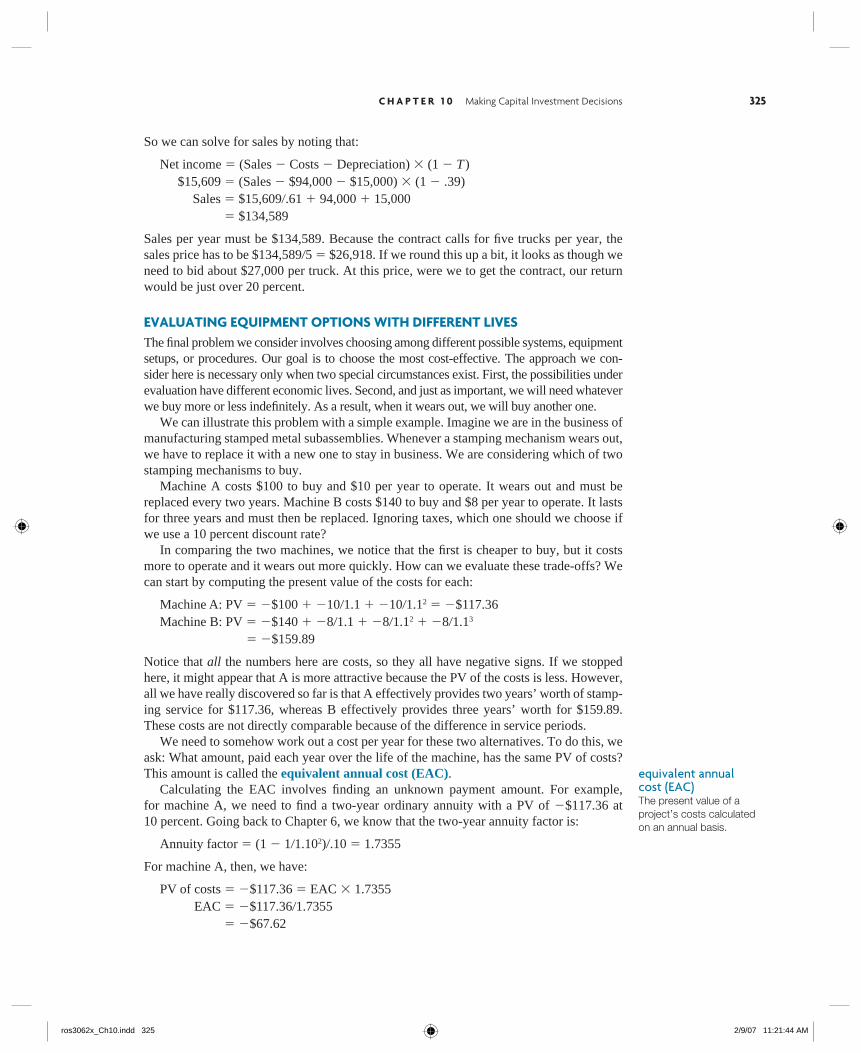
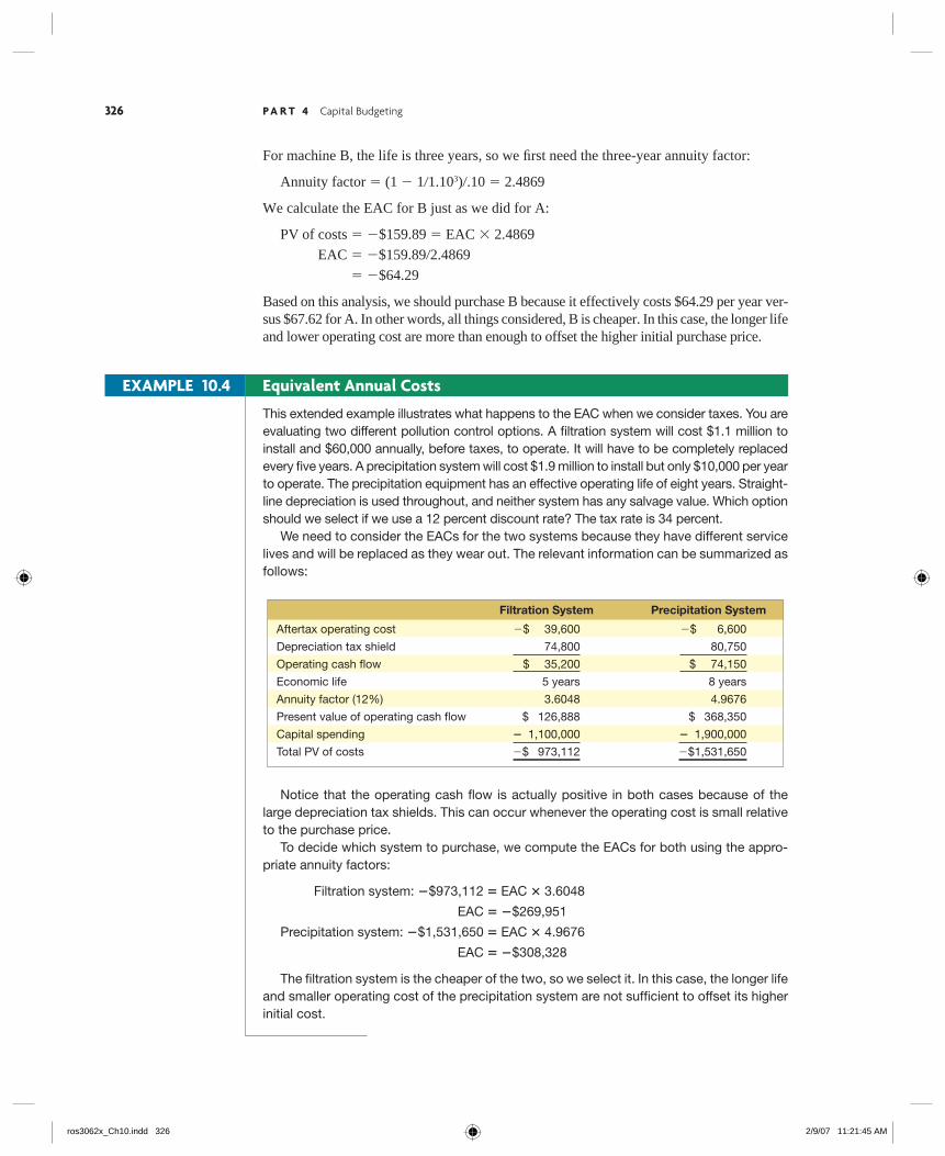
This extended example illustrates what happens to the EAC when we consider taxes. You are evaluating two different pollution control options. A fi ltration system will cost $1.1 million to install and $60,000 annually, before taxes, to operate. It will have to be completely replaced every fi ve years. A precipitation system will cost $1.9 million to install but only $10,000 per year to operate. The precipitation equipment has an effective operating life of eight years. Straight-line depreciation is used throughout, and neither system has any salvage value. Which option should we select if we use a 12 percent discount rate? The tax rate is 34 percent. We need to consider the EACs for the two systems because they have different service lives and will be replaced as they wear out. The relevant information can be summarized as follows:
Filtration System Precipitation System
Aftertax operating cost �$ 39,600 �$ 6,600
Depreciation tax shield 74,800 80,750
Operating cash fl ow $ 35,200 $ 74,150
Economic life 5 years 8 years
Annuity factor (12%) 3.6048 4.9676
Present value of operating cash fl ow $ 126,888 $ 368,350
Capital spending � 1,100,000 � 1,900,000
Total PV of costs �$ 973,112 �$1,531,650
Notice that the operating cash fl ow is actually positive in both cases because of the large depreciation tax shields. This can occur whenever the operating cost is small relative to the purchase price. To decide which system to purchase, we compute the EACs for both using the appro-priate annuity factors:
Filtration system: �$973,112 � EAC � 3.6048
EAC � �$269,951
Precipitation system: �$1,531,650 � EAC � 4.9676
EAC � �$308,328
The fi ltration system is the cheaper of the two, so we select it. In this case, the longer life and smaller operating cost of the precipitation system are not suffi cient to offset its higher initial cost.
EXAMPLE 10.4 Equivalent Annual Costs
ros3062x_Ch10.indd 326ros3062x_Ch10.indd 326 2/9/07 11:21:45 AM2/9/07 11:21:45 AM
C H A P T E R 1 0 Making Capital Investment Decisions 327
Summary and ConclusionsThis chapter has described how to put together a discounted cash fl ow analysis. In it, we covered:
1. The identifi cation of relevant project cash fl ows: We discussed project cash fl ows and described how to handle some issues that often come up, including sunk costs, opportunity costs, fi nancing costs, net working capital, and erosion.
2. Preparing and using pro forma, or projected, fi nancial statements: We showed how information from such fi nancial statements is useful in coming up with projected cash fl ows, and we also looked at some alternative defi nitions of operating cash fl ow.
3. The role of net working capital and depreciation in determining project cash fl ows: We saw that including the change in net working capital was important in cash fl ow analy-sis because it adjusted for the discrepancy between accounting revenues and costs and cash revenues and costs. We also went over the calculation of depreciation expense under current tax law.
4. Some special cases encountered in using discounted cash fl ow analysis: Here we looked at three special issues: evaluating cost-cutting investments, how to go about setting a bid price, and the unequal lives problem.
The discounted cash fl ow analysis we’ve covered here is a standard tool in the business world. It is a very powerful tool, so care should be taken in its use. The most important thing is to identify the cash fl ows in a way that makes economic sense. This chapter gives you a good start in learning to do this.
10.7
10.6a In setting a bid price, we used a zero NPV as our benchmark. Explain why this is appropriate.
10.6b Under what circumstances do we have to worry about unequal economic lives? How do you interpret the EAC?
Concept Questions
CHAPTER REVIEW AND SELF-TEST PROBLEMS
10.1 Capital Budgeting for Project X Based on the following information for proj ect X, should we undertake the venture? To answer, fi rst prepare a pro forma income statement for each year. Next calculate operating cash fl ow. Finish the problem by determining total cash fl ow and then calculating NPV assuming a 28 percent required return. Use a 34 percent tax rate throughout. For help, look back at our shark attractant and power mulcher examples.
Project X involves a new type of graphite composite in-line skate wheel. We think we can sell 6,000 units per year at a price of $1,000 each. Variable costs will run about $400 per unit, and the product should have a four-year life.
Fixed costs for the project will run $450,000 per year. Further, we will need to invest a total of $1,250,000 in manufacturing equipment. This equipment is
Vis
it u
s at
ww
w.m
hhe.
com
/rw
j
ros3062x_Ch10.indd 327ros3062x_Ch10.indd 327 2/9/07 11:21:45 AM2/9/07 11:21:45 AM
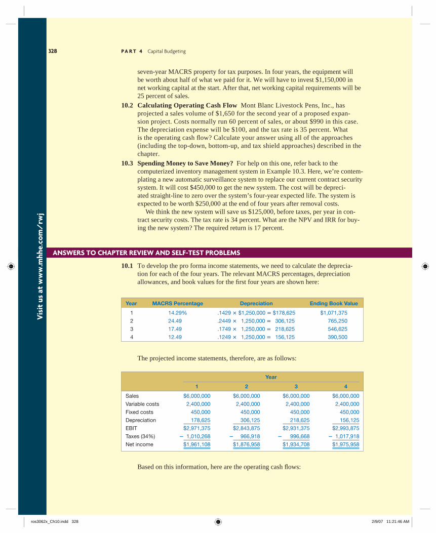
328 P A R T 4 Capital Budgeting
seven-year MACRS property for tax purposes. In four years, the equipment will be worth about half of what we paid for it. We will have to invest $1,150,000 in net working capital at the start. After that, net working capital requirements will be 25 percent of sales.
10.2 Calculating Operating Cash Flow Mont Blanc Livestock Pens, Inc., has projected a sales volume of $1,650 for the second year of a proposed expan-sion project. Costs normally run 60 percent of sales, or about $990 in this case. The depreciation expense will be $100, and the tax rate is 35 percent. What is the operating cash fl ow? Calculate your answer using all of the approaches (including the top-down, bottom-up, and tax shield approaches) described in the chapter.
10.3 Spending Money to Save Money? For help on this one, refer back to the computerized inventory management system in Example 10.3. Here, we’re contem-plating a new automatic surveillance system to replace our current contract security system. It will cost $450,000 to get the new system. The cost will be depreci-ated straight-line to zero over the system’s four-year expected life. The system is expected to be worth $250,000 at the end of four years after removal costs.
We think the new system will save us $125,000, before taxes, per year in con-tract security costs. The tax rate is 34 percent. What are the NPV and IRR for buy-ing the new system? The required return is 17 percent.
ANSWERS TO CHAPTER REVIEW AND SELF-TEST PROBLEMS
10.1 To develop the pro forma income statements, we need to calculate the deprecia-tion for each of the four years. The relevant MACRS percentages, depreciation allowances, and book values for the fi rst four years are shown here:
Year MACRS Percentage Depreciation Ending Book Value
1 14.29% .1429 � $1,250,000 � $178,625 $1,071,375
2 24.49 .2449 � 1,250,000 � 306,125 765,250
3 17.49 .1749 � 1,250,000 � 218,625 546,625
4 12.49 .1249 � 1,250,000 � 156,125 390,500
The projected income statements, therefore, are as follows:
Year
1 2 3 4
Sales $6,000,000 $6,000,000 $6,000,000 $6,000,000
Variable costs 2,400,000 2,400,000 2,400,000 2,400,000
Fixed costs 450,000 450,000 450,000 450,000
Depreciation 178,625 306,125 218,625 156,125
EBIT $2,971,375 $2,843,875 $2,931,375 $2,993,875
Taxes (34%) � 1,010,268 � 966,918 � 996,668 � 1,017,918
Net income $1,961,108 $1,876,958 $1,934,708 $1,975,958
Based on this information, here are the operating cash fl ows:
Vis
it u
s at
ww
w.m
hhe.
com
/rw
j
ros3062x_Ch10.indd 328ros3062x_Ch10.indd 328 2/9/07 11:21:46 AM2/9/07 11:21:46 AM
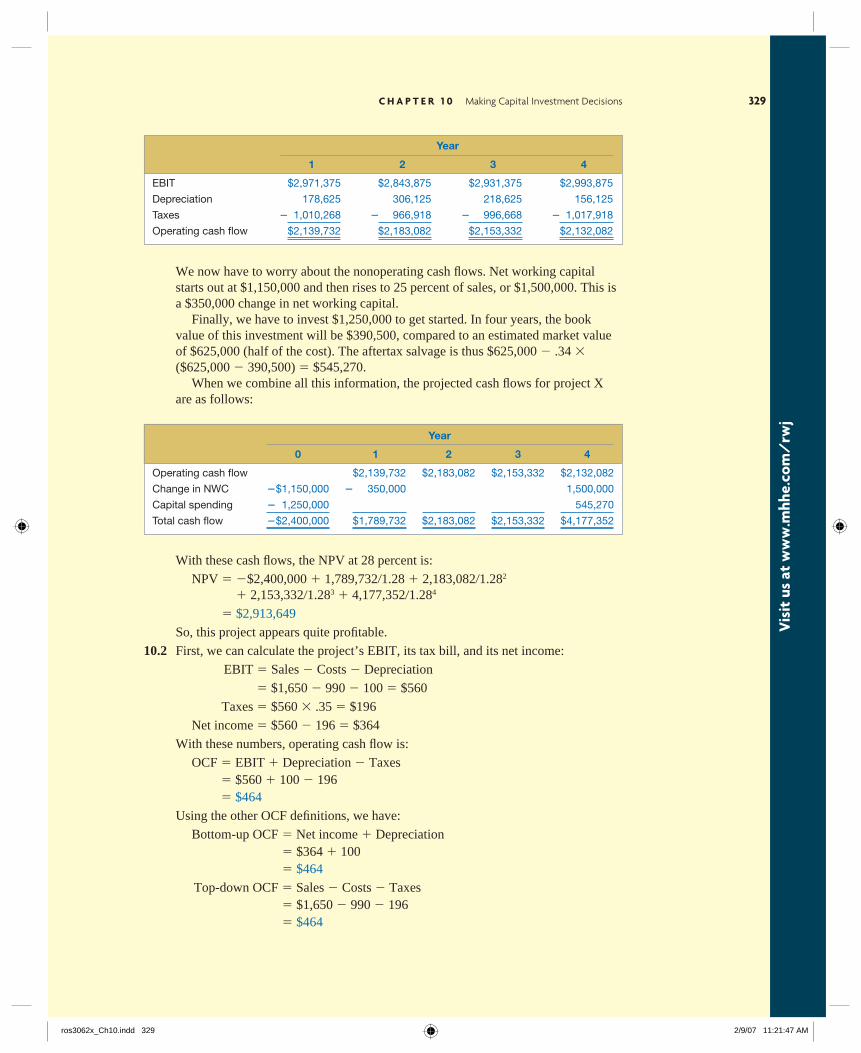
Vis
it u
s at
ww
w.m
hhe.
com
/rw
j
Year
1 2 3 4
EBIT $2,971,375 $2,843,875 $2,931,375 $2,993,875
Depreciation 178,625 306,125 218,625 156,125
Taxes � 1,010,268 � 966,918 � 996,668 � 1,017,918
Operating cash fl ow $2,139,732 $2,183,082 $2,153,332 $2,132,082
We now have to worry about the nonoperating cash fl ows. Net working capital starts out at $1,150,000 and then rises to 25 percent of sales, or $1,500,000. This is a $350,000 change in net working capital.
Finally, we have to invest $1,250,000 to get started. In four years, the book value of this investment will be $390,500, compared to an estimated market value of $625,000 (half of the cost). The aftertax salvage is thus $625,000 � .34 � ($625,000 � 390,500) � $545,270.
When we combine all this information, the projected cash fl ows for project X are as follows:
Year
0 1 2 3 4
Operating cash fl ow $2,139,732 $2,183,082 $2,153,332 $2,132,082
Change in NWC �$1,150,000 � 350,000 1,500,000
Capital spending � 1,250,000 545,270
Total cash fl ow �$2,400,000 $1,789,732 $2,183,082 $2,153,332 $4,177,352
With these cash fl ows, the NPV at 28 percent is:
NPV � �$2,400,000 � 1,789,732�1.28 � 2,183,082�1.282 � 2,153,332�1.283 � 4,177,352�1.284
� $2,913,649
So, this project appears quite profi table.
10.2 First, we can calculate the project’s EBIT, its tax bill, and its net income:
EBIT � Sales � Costs � Depreciation
� $1,650 � 990 � 100 � $560
Taxes � $560 � .35 � $196
Net income � $560 � 196 � $364
With these numbers, operating cash fl ow is:
OCF � EBIT � Depreciation � Taxes � $560 � 100 � 196 � $464
Using the other OCF defi nitions, we have:
Bottom-up OCF � Net income � Depreciation � $364 � 100 � $464
Top-down OCF � Sales � Costs � Taxes � $1,650 � 990 � 196 � $464
C H A P T E R 1 0 Making Capital Investment Decisions 329
ros3062x_Ch10.indd 329ros3062x_Ch10.indd 329 2/9/07 11:21:47 AM2/9/07 11:21:47 AM
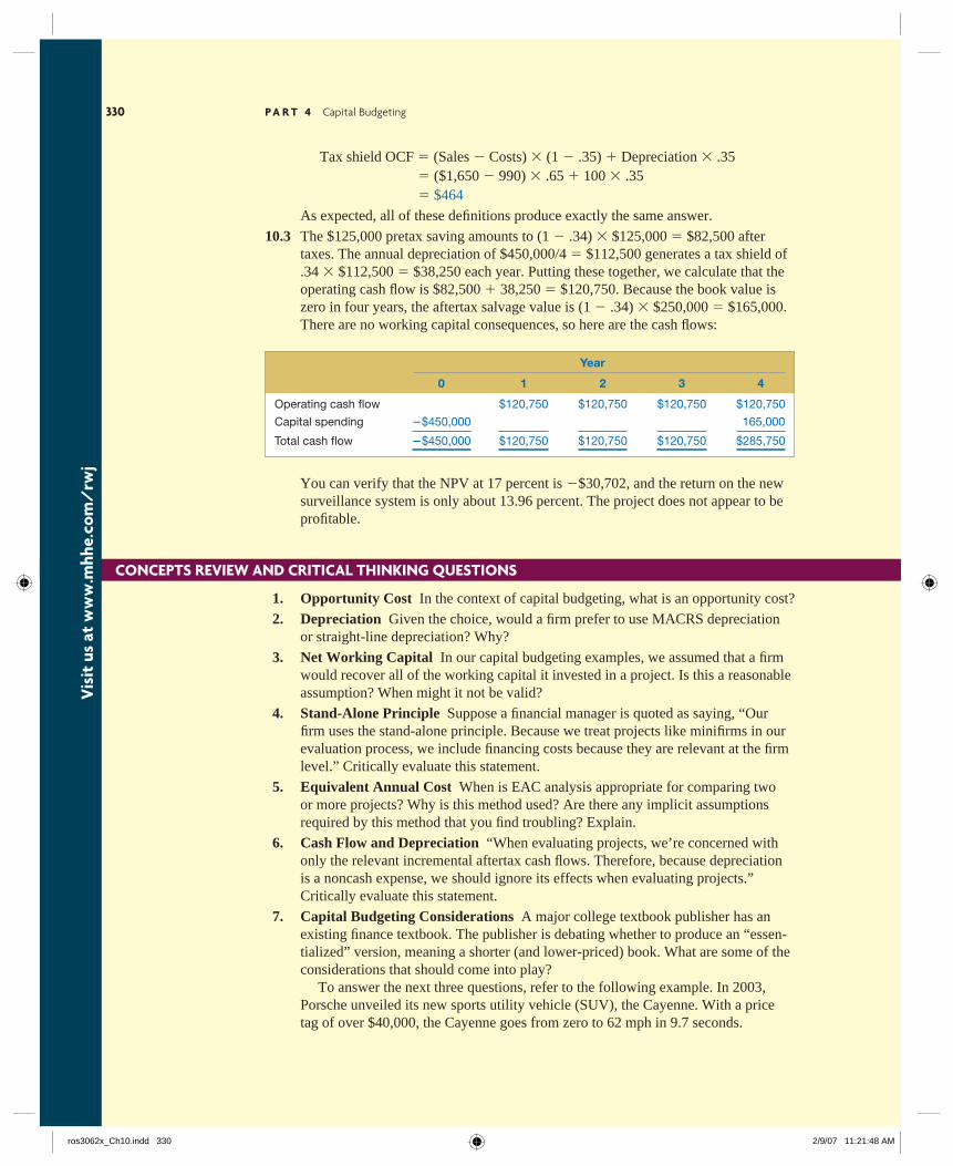
330 P A R T 4 Capital Budgeting
Tax shield OCF � (Sales � Costs) � (1 � .35) � Depreciation � .35 � ($1,650 � 990) � .65 � 100 � .35 � $464
As expected, all of these defi nitions produce exactly the same answer.
10.3 The $125,000 pretax saving amounts to (1 � .34) � $125,000 � $82,500 after taxes. The annual depreciation of $450,000�4 � $112,500 generates a tax shield of .34 � $112,500 � $38,250 each year. Putting these together, we calculate that the operating cash fl ow is $82,500 � 38,250 � $120,750. Because the book value is zero in four years, the aftertax salvage value is (1 � .34) � $250,000 � $165,000. There are no working capital consequences, so here are the cash fl ows:
Year
0 1 2 3 4
Operating cash fl ow $120,750 $120,750 $120,750 $120,750
Capital spending �$450,000 165,000
Total cash fl ow �$450,000 $120,750 $120,750 $120,750 $285,750
You can verify that the NPV at 17 percent is �$30,702, and the return on the new surveillance system is only about 13.96 percent. The project does not appear to be profi table.
CONCEPTS REVIEW AND CRITICAL THINKING QUESTIONS
Vis
it u
s at
ww
w.m
hhe.
com
/rw
j
1. Opportunity Cost In the context of capital budgeting, what is an opportunity cost?
2. Depreciation Given the choice, would a fi rm prefer to use MACRS depreciation or straight-line depreciation? Why?
3. Net Working Capital In our capital budgeting examples, we assumed that a fi rm would recover all of the working capital it invested in a project. Is this a reasonable assumption? When might it not be valid?
4. Stand-Alone Principle Suppose a fi nancial manager is quoted as saying, “Our fi rm uses the stand-alone principle. Because we treat projects like minifi rms in our evaluation process, we include fi nancing costs because they are relevant at the fi rm level.” Critically evaluate this statement.
5. Equivalent Annual Cost When is EAC analysis appropriate for comparing two or more projects? Why is this method used? Are there any implicit assumptions required by this method that you fi nd troubling? Explain.
6. Cash Flow and Depreciation “When evaluating projects, we’re concerned with only the relevant incremental aftertax cash fl ows. Therefore, because depreciation is a noncash expense, we should ignore its effects when evaluating projects.” Critically evaluate this statement.
7. Capital Budgeting Considerations A major college textbook publisher has an existing fi nance textbook. The publisher is debating whether to produce an “essen-tialized” version, meaning a shorter (and lower-priced) book. What are some of the considerations that should come into play?
To answer the next three questions, refer to the following example. In 2003, Porsche unveiled its new sports utility vehicle (SUV), the Cayenne. With a price tag of over $40,000, the Cayenne goes from zero to 62 mph in 9.7 seconds.
ros3062x_Ch10.indd 330ros3062x_Ch10.indd 330 2/9/07 11:21:48 AM2/9/07 11:21:48 AM
C H A P T E R 1 0 Making Capital Investment Decisions 331
Porsche’s decision to enter the SUV market was a response to the runaway success of other high-priced SUVs such as the Mercedes-Benz M-class. Vehicles in this class had generated years of high profi ts. The Cayenne certainly spiced up the mar-ket, and Porsche subsequently introduced the Cayenne Turbo S, which goes from zero to 60 mph in 4.8 seconds and has a top speed of 168 mph. The price tag for the Cayenne Turbo S in 2006? About $112,000!
Some analysts questioned Porsche’s entry into the luxury SUV market. The ana-lysts were concerned not only that Porsche was a late entry into the market, but also that the introduction of the Cayenne would damage Porsche’s reputation as a maker of high-performance automobiles.
8. Erosion In evaluating the Cayenne, would you consider the possible damage to Porsche’s reputation erosion?
9. Capital Budgeting Porsche was one of the last manufacturers to enter the sports utility vehicle market. Why would one company decide to proceed with a product when other companies, at least initially, decide not to enter the market?
10. Capital Budgeting In evaluating the Cayenne, what do you think Porsche needs to assume regarding the substantial profi t margins that exist in this market? Is it likely they will be maintained as the market becomes more competitive, or will Porsche be able to maintain the profi t margin because of its image and the performance of the Cayenne?
QUESTIONS AND PROBLEMS
BASIC(Questions 1–18)
1. Relevant Cash Flows Parker & Stone, Inc., is looking at setting up a new manufacturing plant in South Park to produce garden tools. The company bought some land six years ago for $5 million in anticipation of using it as a warehouse and distribution site, but the company has since decided to rent these facilities from a competitor instead. If the land were sold today, the company would net $5.3 million. The company wants to build its new manufacturing plant on this land; the plant will cost $11.6 million to build, and the site requires $425,000 worth of grading before it is suitable for construction. What is the proper cash fl ow amount to use as the initial investment in fi xed assets when evaluating this project? Why?
2. Relevant Cash Flows Winnebagel Corp. currently sells 30,000 motor homes per year at $45,000 each, and 12,000 luxury motor coaches per year at $85,000 each. The company wants to introduce a new portable camper to fi ll out its product line; it hopes to sell 19,000 of these campers per year at $12,000 each. An independent consultant has determined that if Winnebagel introduces the new campers, it should boost the sales of its existing motor homes by 4,500 units per year, and reduce the sales of its motor coaches by 900 units per year. What is the amount to use as the annual sales fi gure when evaluating this project? Why?
3. Calculating Projected Net Income A proposed new investment has projected sales of $740,000. Variable costs are 60 percent of sales, and fi xed costs are $173,000; depreciation is $75,000. Prepare a pro forma income statement assuming a tax rate of 35 percent. What is the projected net income?
Vis
it u
s at
ww
w.m
hhe.
com
/rw
j
ros3062x_Ch10.indd 331ros3062x_Ch10.indd 331 2/9/07 11:21:48 AM2/9/07 11:21:48 AM
Vis
it u
s at
ww
w.m
hhe.
com
/rw
j332 P A R T 4 Capital Budgeting
4. Calculating OCF Consider the following income statement:
Sales $876,400 Costs 547,300 Depreciation 128,000 EBIT ? Taxes (34%) ? Net income ?
Fill in the missing numbers and then calculate the OCF. What is the depreciation tax shield?
5. OCF from Several Approaches A proposed new project has projected sales of $96,000, costs of $49,000, and depreciation of $4,500. The tax rate is 35 percent. Calculate operating cash fl ow using the four different approaches described in the chapter and verify that the answer is the same in each case.
6. Calculating Depreciation A piece of newly purchased industrial equipment costs $925,000 and is classifi ed as seven-year property under MACRS. Calculate the annual depreciation allowances and end-of-the-year book values for this equipment.
7. Calculating Salvage Value Consider an asset that costs $468,000 and is depreciated straight-line to zero over its eight-year tax life. The asset is to be used in a fi ve-year project; at the end of the project, the asset can be sold for $72,000. If the relevant tax rate is 35 percent, what is the aftertax cash fl ow from the sale of this asset?
8. Calculating Salvage Value An asset used in a four-year project falls in the fi ve-year MACRS class for tax purposes. The asset has an acquisition cost of $8,400,000 and will be sold for $1,750,000 at the end of the project. If the tax rate is 35 percent, what is the aftertax salvage value of the asset?
9. Calculating Project OCF Phone Home, Inc., is considering a new three-year expan-sion project that requires an initial fi xed asset investment of $4.2 million. The fi xed asset will be depreciated straight-line to zero over its three-year tax life, after which time it will be worthless. The project is estimated to generate $3,100,000 in annual sales, with costs of $990,000. If the tax rate is 35 percent, what is the OCF for this project?
10. Calculating Project NPV In the previous problem, suppose the required return on the project is 12 percent. What is the project’s NPV?
11. Calculating Project Cash Flow from Assets In the previous problem, suppose the project requires an initial investment in net working capital of $300,000, and the fi xed asset will have a market value of $210,000 at the end of the proj ect. What is the project’s year 0 net cash fl ow? Year 1? Year 2? Year 3? What is the new NPV?
12. NPV and Modifi ed ACRS In the previous problem, suppose the fi xed asset actu-ally falls into the three-year MACRS class. All the other facts are the same. What is the project’s year 1 net cash fl ow now? Year 2? Year 3? What is the new NPV?
13. Project Evaluation Dog Up! Franks is looking at a new sausage system with an installed cost of $440,000. This cost will be depreciated straight-line to zero over the project’s fi ve-year life, at the end of which the sausage system can be scrapped for $60,000. The sausage system will save the fi rm $130,000 per year in pretax operating costs, and the system requires an initial investment in net working capital of $34,000. If the tax rate is 34 percent and the discount rate is 10 percent, what is the NPV of this project?
14. Project Evaluation Your fi rm is contemplating the purchase of a new $840,000 computer-based order entry system. The system will be depreciated straight-line to
ros3062x_Ch10.indd 332ros3062x_Ch10.indd 332 2/9/07 11:21:49 AM2/9/07 11:21:49 AM
Vis
it u
s at
ww
w.m
hhe.
com
/rw
j
C H A P T E R 1 0 Making Capital Investment Decisions 333
zero over its fi ve-year life. It will be worth $75,000 at the end of that time. You will save $330,000 before taxes per year in order processing costs, and you will be able to reduce working capital by $125,000 (this is a one-time reduction). If the tax rate is 35 percent, what is the IRR for this project?
15. Project Evaluation In the previous problem, suppose your required return on the project is 20 percent and your pretax cost savings are $380,000 per year. Will you accept the project? What if the pretax cost savings are $280,000 per year? At what level of pretax cost savings would you be indifferent between accepting the project and not accepting it?
16. Calculating EAC A fi ve-year project has an initial fi xed asset investment of $240,000, an initial NWC investment of $20,000, and an annual OCF of �$32,000. The fi xed asset is fully depreciated over the life of the project and has no salvage value. If the required return is 11 percent, what is this project’s equivalent annual cost, or EAC?
17. Calculating EAC You are evaluating two different silicon wafer milling machines. The Techron I costs $330,000, has a three-year life, and has pretax operating costs of $41,000 per year. The Techron II costs $480,000, has a fi ve-year life, and has pretax operating costs of $33,000 per year. For both milling machines, use straight-line depreciation to zero over the project’s life and assume a salvage value of $20,000. If your tax rate is 35 percent and your discount rate is 14 percent, compute the EAC for both machines. Which do you prefer? Why?
18. Calculating a Bid Price Heer Enterprises needs someone to supply it with 160,000 cartons of machine screws per year to support its manufacturing needs over the next fi ve years, and you’ve decided to bid on the contract. It will cost you $840,000 to install the equipment necessary to start production; you’ll depreciate this cost straight-line to zero over the project’s life. You estimate that in fi ve years, this equipment can be salvaged for $60,000. Your fi xed production costs will be $290,000 per year, and your variable production costs should be $8.50 per carton. You also need an initial investment in net working capital of $75,000. If your tax rate is 35 percent and you require a 12 percent return on your investment, what bid price should you submit?
19. Cost-Cutting Proposals Chatman Machine Shop is considering a four-year proj-ect to improve its production effi ciency. Buying a new machine press for $530,000 is estimated to result in $205,000 in annual pretax cost savings. The press falls in the MACRS fi ve-year class, and it will have a salvage value at the end of the proj-ect of $90,000. The press also requires an initial investment in spare parts inventory of $20,000, along with an additional $3,000 in inventory for each succeeding year of the project. If the shop’s tax rate is 35 percent and its discount rate is 9 percent, should Chatman buy and install the machine press?
20. Comparing Mutually Exclusive Projects Eads Industrial Systems Company (EISC) is trying to decide between two different conveyor belt systems. System A costs $380,000, has a four-year life, and requires $105,000 in pretax annual op erating costs. System B costs $490,000, has a six-year life, and requires $90,000 in pretax annual operating costs. Both systems are to be depreciated straight-line to zero over their lives and will have zero salvage value. Whichever project is cho-sen, it will not be replaced when it wears out. If the tax rate is 34 percent and the discount rate is 13 percent, which project should the fi rm choose?
21. Comparing Mutually Exclusive Projects Suppose in the previous problem that EISC always needs a conveyor belt system; when one wears out, it must be replaced. Which project should the fi rm choose now?
INTERMEDIATE(Questions 19–24)
ros3062x_Ch10.indd 333ros3062x_Ch10.indd 333 2/9/07 11:21:50 AM2/9/07 11:21:50 AM
Vis
it u
s at
ww
w.m
hhe.
com
/rw
j334 P A R T 4 Capital Budgeting
22. Calculating a Bid Price Consider a project to supply 100 million postage stamps per year to the U.S. Postal Service for the next fi ve years. You have an idle parcel of land available that cost $1,000,000 fi ve years ago; if the land were sold today, it would net you $1,200,000 aftertax. The land can be sold for $1,500,000 after taxes in fi ve years. You will need to install $3.8 million in new manufacturing plant and equipment to actually produce the stamps; this plant and equipment will be depreci-ated straight-line to zero over the project’s fi ve-year life. The equipment can be sold for $650,000 at the end of the project. You will also need $500,000 in initial net working capital for the project, and an additional investment of $50,000 in every year thereafter. Your production costs are 0.5 cents per stamp, and you have fi xed costs of $900,000 per year. If your tax rate is 34 percent and your required return on this project is 12 percent, what bid price should you submit on the contract?
23. Interpreting a Bid Price In the previous problem, suppose you were going to use a three-year MACRS depreciation schedule for your manufacturing equipment, and you could keep working capital investments down to only $25,000 per year. How would this new information affect your calculated bid price?
24. Comparing Mutually Exclusive Projects Vandalay Industries is considering the purchase of a new machine for the production of latex. Machine A costs $2,600,000 and will last for six years. Variable costs are 35 percent of sales, and fi xed costs are $160,000 per year. Machine B costs $4,900,000 and will last for nine years. Vari-able costs for this machine are 30 percent of sales and fi xed costs are $110,000 per year. The sales for each machine will be $9 million per year. The required return is 10 percent, and the tax rate is 35 percent. Both machines will be depreciated on a straight-line basis. If the company plans to replace the machine when it wears out on a perpetual basis, which machine should you choose?
25. Calculating Project NPV You have been hired as a consultant for Pristine Urban-Tech Zither, Inc. (PUTZ), manufacturers of fi ne zithers. The market for zithers is growing quickly. The company bought some land three years ago for $1 million in anticipation of using it as a toxic waste dump site but has recently hired another company to handle all toxic materials. Based on a recent appraisal, the company believes it could sell the land for $800,000 on an aftertax basis. In four years, the land could be sold for $1 million after taxes. The company also hired a marketing fi rm to analyze the zither market, at a cost of $125,000. An excerpt of the marketing report is as follows:
The zither industry will have a rapid expansion in the next four years. With the brand name recognition that PUTZ brings to bear, we feel that the company will be able to sell 2,900, 3,800, 2,700, and 1,900 units each year for the next four years, respectively. Again, capitalizing on the name recognition of PUTZ, we feel that a premium price of $700 can be charged for each zither. Because zithers appear to be a fad, we feel at the end of the four-year period, sales should be discontinued.
PUTZ believes that fi xed costs for the project will be $350,000 per year, and vari-able costs are 15 percent of sales. The equipment necessary for production will cost $3.8 million and will be depreciated according to a three-year MACRS schedule. At the end of the project, the equipment can be scrapped for $400,000. Net work-ing capital of $120,000 will be required by the end of the fi rst year. PUTZ has a 38 percent tax rate, and the required return on the project is 13 percent. What is the NPV of the project? Assume the company has other profi table projects.
26. Project Evaluation Aguilera Acoustics (AAI), Inc., projects unit sales for a new seven-octave voice emulation implant as follows:
CHALLENGE(Questions 25–30)
ros3062x_Ch10.indd 334ros3062x_Ch10.indd 334 2/9/07 11:21:50 AM2/9/07 11:21:50 AM
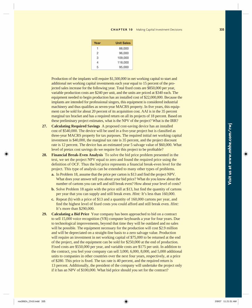
Vis
it u
s at
ww
w.m
hhe.
com
/rw
j
C H A P T E R 1 0 Making Capital Investment Decisions 335
Year Unit Sales
1 88,000
2 96,000
3 109,000
4 118,000
5 95,000
Production of the implants will require $1,500,000 in net working capital to start and additional net working capital investments each year equal to 15 percent of the pro-jected sales increase for the following year. Total fi xed costs are $850,000 per year, variable production costs are $240 per unit, and the units are priced at $340 each. The equipment needed to begin production has an installed cost of $22,000,000. Because the implants are intended for professional singers, this equipment is considered industrial machinery and thus qualifi es as seven-year MACRS property. In fi ve years, this equip-ment can be sold for about 20 percent of its acquisition cost. AAI is in the 35 percent marginal tax bracket and has a required return on all its projects of 18 percent. Based on these preliminary project estimates, what is the NPV of the project? What is the IRR?
27. Calculating Required Savings A proposed cost-saving device has an installed cost of $540,000. The device will be used in a fi ve-year project but is classifi ed as three-year MACRS property for tax purposes. The required initial net working capital investment is $40,000, the marginal tax rate is 35 percent, and the project discount rate is 12 percent. The device has an estimated year 5 salvage value of $60,000. What level of pretax cost savings do we require for this project to be profi table?
28. Financial Break-Even Analysis To solve the bid price problem presented in the text, we set the project NPV equal to zero and found the required price using the defi nition of OCF. Thus the bid price represents a fi nancial break-even level for the project. This type of analysis can be extended to many other types of problems.
a. In Problem 18, assume that the price per carton is $13 and find the project NPV. What does your answer tell you about your bid price? What do you know about the number of cartons you can sell and still break even? How about your level of costs?
b. Solve Problem 18 again with the price still at $13, but fi nd the quantity of cartons per year that you can supply and still break even. Hint: It’s less than 160,000.
c. Repeat (b) with a price of $13 and a quantity of 160,000 cartons per year, and fi nd the highest level of fi xed costs you could afford and still break even. Hint: It’s more than $290,000.
29. Calculating a Bid Price Your company has been approached to bid on a contract to sell 15,000 voice recognition (VR) computer keyboards a year for four years. Due to technological improvements, beyond that time they will be outdated and no sales will be possible. The equipment necessary for the production will cost $2.9 million and will be depreciated on a straight-line basis to a zero salvage value. Production will require an investment in net working capital of $75,000 to be returned at the end of the project, and the equipment can be sold for $250,000 at the end of production. Fixed costs are $550,000 per year, and variable costs are $175 per unit. In addition to the contract, you feel your company can sell 3,000, 6,000, 8,000, and 5,000 additional units to companies in other countries over the next four years, respectively, at a price of $280. This price is fi xed. The tax rate is 40 percent, and the required return is 13 percent. Additionally, the president of the company will undertake the project only if it has an NPV of $100,000. What bid price should you set for the contract?
ros3062x_Ch10.indd 335ros3062x_Ch10.indd 335 2/9/07 11:21:51 AM2/9/07 11:21:51 AM
336 P A R T 4 Capital Budgeting
30. Replacement Decisions Suppose we are thinking about replacing an old computer with a new one. The old one cost us $360,000; the new one will cost $730,000. The new machine will be depreciated straight-line to zero over its fi ve-year life. It will probably be worth about $135,000 after fi ve years.
The old computer is being depreciated at a rate of $120,000 per year. It will be completely written off in three years. If we don’t replace it now, we will have to replace it in two years. We can sell it now for $190,000; in two years, it will prob-ably be worth $80,000. The new machine will save us $130,000 per year in operat-ing costs. The tax rate is 38 percent, and the discount rate is 14 percent.
a. Suppose we recognize that if we don’t replace the computer now, we will be replac-ing it in two years. Should we replace now or should we wait? Hint: What we effec-tively have here is a decision either to “invest” in the old computer (by not selling it) or to invest in the new one. Notice that the two investments have unequal lives.
b. Suppose we consider only whether we should replace the old computer now without worrying about what’s going to happen in two years. What are the relevant cash fl ows? Should we replace it or not? Hint: Consider the net change in the fi rm’s aftertax cash fl ows if we do the replacement.
MINICASE
Conch Republic Electronics, Part 1Conch Republic Electronics is a midsized electronics manu-facturer located in Key West, Florida. The company president is Shelley Couts, who inherited the company. When it was founded over 70 years ago, the company originally repaired radios and other household appliances. Over the years, the company expanded into manufacturing and is now a reputa-ble manufacturer of various electronic items. Jay McCanless, a recent MBA graduate, has been hired by the company’s fi nance department. One of the major revenue-producing items manufactured by Conch Republic is a personal digital assistant (PDA). Conch Republic currently has one PDA model on the mar-ket, and sales have been excellent. The PDA is a unique item in that it comes in a variety of tropical colors and is prepro-grammed to play Jimmy Buffett music. However, as with any electronic item, technology changes rapidly, and the current PDA has limited features in comparison with newer models. Conch Republic spent $750,000 to develop a prototype for a new PDA that has all the features of the existing PDA but adds new features such as cell phone capability. The company has spent a further $200,000 for a marketing study to determine the expected sales fi gures for the new PDA. Conch Republic can manufacture the new PDA for $150 each in variable costs. Fixed costs for the operation are esti-mated to run $4.5 million per year. The estimated sales vol-ume is 70,000, 80,000, 100,000, 85,000, and 75,000 per each year for the next fi ve years, respectively. The unit price of
the new PDA will be $340. The necessary equipment can be purchased for $16.5 million and will be depreciated on a seven-year MACRS schedule. It is believed the value of the equipment in fi ve years will be $3.5 million. As previously stated, Conch Republic currently manufac-tures a PDA. Production of the existing model is expected to be terminated in two years. If Conch Republic does not intro-duce the new PDA, sales will be 80,000 units and 60,000 units for the next two years, respectively. The price of the existing PDA is $280 per unit, with variable costs of $120 each and fi xed costs of $1,800,000 per year. If Conch Republic does introduce the new PDA, sales of the existing PDA will fall by 15,000 units per year, and the price of the existing units will have to be lowered to $240 each. Net working capital for the PDAs will be 20 percent of sales and will occur with the timing of the cash fl ows for the year; for example, there is no initial outlay for NWC, but changes in NWC will fi rst occur in year 1 with the fi rst year’s sales. Conch Republic has a 35 percent corporate tax rate and a 12 percent required return. Shelly has asked Jay to prepare a report that answers the following questions:
1. What is the payback period of the project?
2. What is the profi tability index of the project?
3. What is the IRR of the project?
4. What is the NPV of the project?
Vis
it u
s at
ww
w.m
hhe.
com
/rw
j
ros3062x_Ch10.indd 336ros3062x_Ch10.indd 336 2/9/07 11:21:52 AM2/9/07 11:21:52 AM
Related Documents