Major League Soccer Scheduling Problem - CMU · Major League Soccer Scheduling Problem Canto Zhu, Muchen Zhou, Qiuyi Jia, Xiang Luo Dec.16 2016 1 Introduction Major League Soccer

Major League Soccer Scheduling Problem

Canto Zhu, Muchen Zhou, Qiuyi Jia, Xiang Luo

Dec.16 2016

1 Introduction

Major League Soccer is the highest level mens professional soccer league in United States and Canada, con-sisting of 20 teams, with 17 in United States and 3 in Canada. The League is divided by two Conferences:Western and Eastern with 10 teams each. The regular season of the League runs from early March to lateOctober each year. It is important to look at MLS mainly for three reasons. Firstly, it is a fast-growingleague, with only 10 teams competed in 1996 when the League started. Secondly, the popularity of the gamehas increased dramatically, with the average per-game attendance in MLS increased by 40% in the pastdecade, which exceeds that of NHL and NBA. Lastly, the big TV broadcasting contract signed with ESPN,Fox Sports, and Univision has demonstrated the huge commercial value of the League.

Our model aims to make an efficient schedule that balances the travel distance, opponent strength, andgame attractiveness of each team and game weeks. We will use integer programming to achieve theseoptimizing goals.

2 Rules

Each team in the League will play a total of 34 games in the regular season. 24 games are intra-conferenceand 10 are cross-conference games. The 10 cross-conference games are scheduled as 5 home and 5 away andswitch home-away schedule year by year. Among the 24 intra-conference games, 18 of which are scheduledas double round robin with other 9 teams within the conference. The rest are 6 additional intra-conferencegames, 3 home and 3 away with different opponents.

Our model will focus on the Western Conference since there are larger distance differences between cities.Once we solved one conference, it will be relatively simple to repeat the same process on the other conference.

3 Data

We collected several kinds of data for our model. The data for distance are from distance24 API to acquire thedirect distance between cities in North America. As for the calculation of fairness, we used team valuationsreleased by Forbes in 2016 for team value, past two years average winning percentages (one year for newly-formed teams) for the winning rate, and attendance percentage instead of capacity rate for attendance rateas a way to measure fans enthusiasm for their teams. All results are normalized.

1

4 Assumptions

1. Assume that no team plays more than one game per week.

A regular MLS seasons is played between March and October, with a span of roughly thirty weeks, andtypically on the weekends. Since each team has to play 34 games in total, we assume that that thereare 34 weeks so that no team plays more than once per week. In real schedules, there might be lessweeks so that some teams have to play twice in a week. MLS solves this problem by adding mid-weekgames on Wednesdays and Thursdays, which we will address in later parts of this paper. In brief, ourproject solves the 34 week problem by integer programming, then adapts it to real life schedule bymanually adding the additional mid-week games.

2. Assume that after each game, teams always return to their home city.

Following Assumption 1, we further assume that every away team returns to its home city after eachgame, since they would have enough time to rest between games. The greatest benefit it brings is thesimplicity in calculating travelling distances for a game, which is just the distance between home citiesof the two matching teams.

5 Optimization Goals

1. Minimizing total traveling distance for the 6 additional games

For the purpose of optimization, we are only trying to optimize the total traveling distance for the 6additional intra-conference games for the nature of its relative randomness. Since the other 18 intra-conference games are fixed in distance, and the other 10 cross-conference games are fixed in distance ina two-year span with home and away schedules taking turns each year, there is no need to optimize theirdistances. Similar optimization problem is the traveling tournament problem (TTP) introduced in theseminal paper of Easton et al. (2001). It is a challenging combinatorial optimization problem in sportsscheduling that derives the most significant aspects of traveling distances constraints in scheduling atimetable.

2. Home-away balance and Fairness

Besides distance optimization, we are also trying to achieve a home-away balance to ensure that noteam plays too many consecutive home games or away games. To achieve fairness for each team, wewant to balance the strength of each team’s opponents. That is, no team is playing with too manystrong teams nor too many weak teams. The strength of each team is determined by its averagewinning rate in the past two seasons. Our fairness balance is calculated by a normalized weighted sumof team value, game attendance rate, and historical winning rate.

3. Attractiveness

As for the attractiveness of the games, we adhere to realistic situation by considering special weeksand holidays, such as July the Fourth, and conflicts with other popular sports for scheduling moreattractive games. Besides, we take individual team’s opponents into consideration for attractiveness.For example, when LA plays against San Jose, it might be a lot more attractive since it’s a famousrivalry called California Clasico. We are also considering the weather effect in which for the first twoweeks’ games, we try to have the season open with some of the more warm-climate teams hosting, forinstance, eastern teams will play more aways at western teams’ homes.

2

6 Formulation

This section presents the formulation to the distance-minimizing optimization problem.

6.1 Definitions

Define T = 10 as there are 10 teams in both the Western Conference and the Eastern Conference.Define K = 34 as there are 34 games (weeks) to be scheduled.

There are three categories of variables: distance variables, attractiveness variables, and decision variables.

6.1.1 Distance variables

There is a distance associated to each pair of teams, corresponding to the distance between their home cities.Given a number T of teams, distances dij between the home cities of teams i and j, for every i, j = 1, . . . , Tare the flight distance between the two cities, with dij = 0 if i = j. The flight distances are collected fromonline resources.

6.1.2 Fairness and Attractiveness variables

There is a fairness value associated to each team, calculated by the weighted sum of winning rate, attendancerate, and commercial value of the team. It represents the strength of a team, but the product of such value ofthe two teams is also a good indicator of attractiveness of a game. Although other factors may also influencegame attractiveness, this is easier to be quantified and compared.

Given a number of T of teams, fairness ai of team i, for every i = 1, . . . , T are w1 × αi +w2 × βi +w3 × γi,where w1 is the weight for winning rate, w2 is the weight for attendance rate, and w3 is the weight forcommercial value, and αi is the normalized winning rate of team i, βi is the normalized attendance rate ofteami, and γi is the normalized commercial value of team i.

Currently, we set w1 = 13 , w2 = 1

3 , and w3 = 13 . These values are based on estimations of how much

each category contributes to strength of a team.

In addition, there is an fairnes/attractiveness value associated to each game, calculated by the productof the fairness value of the opposing teams. Given a number T of teams, fairness Aij of the game betweenteam i and j, for every i = 1, . . . , T are ai × aj . We ensure the fairness value of each game is within certainrange.

6.1.3 Decision variables

There are three sets of decision variables for three distinctive components of the set of games to be scheduled:

(1) xijk: the 6 additional games within conference

(2) yijk: the 10 games across conference

(3) zijk: the 18 regular games within conference

and xijk, yijk, zijk ∈ {0, 1}, where 1 indicates if team i plays away with team j at week k and 0 otherwise.

Note i, j ∈ [T ] for x, z while i, j ∈ [2T ] for y since x and z concern with only games within conferencegames while y concerns also with games across conference games, and k ∈ [K].

3

6.1.4 Summary of all variables

In summary, we define the following variables:

· dij := distance between the home of team i and team j

· αi := normalized winning rate of team i

· βi := normalized attendance rate of teami

· γi := normalized commercial value of team i

· ai := the weighted coefficient of winning rate, attendance rate, and commercial value of team i wherewj := the weight for winning rate, attendance rate, and commercial value in calculation of fairnessai is calculated by ai = w1 × αi + w2 × βi + w3 × γi

· For the 6 additional games, xijk =

{1, if team i plays away with team j at week k

0, otherwise

· For the 10 games across conference, yijk =


0, otherwise

· For the 18 regular games within conference, zijk =


0, otherwise

where i, j are indices of teams, i, j ∈ [T ] for x, z (within conference) and i, j ∈ [2T ] for y (across conference), and k is index of weeks, k ∈ [K].

6.2 Integer Programming Problem

The integer programming problem can be formulated according to MLS rules and variable definitions asfollows:

• Objective function

The objective is to minimize the total distance traveled by all teams:

min∑k

∑i

∑j

dijxijk i, j ∈ [T ], k ∈ [K]

• Constraints

– Constraints concerned with all x, y, z:

(1) Distance from and to the same city is 0:

diik = 0 ∀i, k

(2) Each team does not play with itself:

xiik = 0, yiik = 0, ziik = 0 ∀i, k

(3) Each team plays at most once per week:∑j

(xijk + xjik + yijk + yjik + zijk + zjik) ≤ 1 ∀i, k

4

(4) Ensure attractiveness for each week’s games is above some threshold P :∑i

∑j

(ai × aj)(xijk + yijk + zijk) ≥ P ∀k

– Constraints concerned with only x:

(5) Each team plays 3 home, 3 away additional games within conference:∑i

∑k

xijk = 3 ∀j,∑j

∑k

xijk = 3 ∀i

(6) Any two teams play at most once additionally:∑j

(xijk + xjik) ≤ 1 ∀i, k

(7) Ensure fairness is within range [L,U ]:

L ≤∑k

∑i

αi(xijk + xjik) ≤ U ∀j

– Constraints concerned with only y:

(8) Each team plays 5 home, 5 away games across conference:∑j

∑k

yijk = 5 ∀i,∑i

∑k

yijk = 5 ∀j

(9) Any two teams across conference play one game:∑j

(yijk + yjik) = 1 ∀i, k

– Constraints concerned with only z:

(10) Each team plays 9 home, 9 away regular games within conference:∑j

∑k

zijk = 9 ∀i,∑j

∑k

zijk = 9 ∀j

(11) Any two teams play 1 home, 1 away games:∑k

zijk = 1 and∑k

zjik = 1 ∀i, j

where xijk, yijk, zijk ∈ {0, 1}.

7 Implementation

After exploring various tools, we use Matlab as the integer programming solver, since it outperforms manyother tools (mainly in terms of runtime) with our large problem scale. Matlab also has well-documentedinteger programming solver libraries.

This section discusses some core implementation details.

5

7.1 Generate constants, distance, fairness, and winning rate

Set the values of T , K, distance, fairness, and winning rate.

1 M = csvread(‘Data - Basic Info.csv ’); % distance

2 A = csvread(‘Data - Fairness.csv ’); % fairness

3 w = csvread(‘Data - WinningRate.csv ’); % winning rate

45 T = 10; % number of teams

6 K = 34; % number of games/weeks

The distance data, fairness data, and winning rate data are collected from online resources and calculatedas explained in variable definitions.

Note M(i,j) in code correspondes to dij in this paper, A(i) in code correspondes to ai in this paper,and w(i) correspondes to αi in this paper. The naming is slightly different in code for better readability.

7.2 Generate objective and constraint matrices and vectors

The objective function vector obj in intlincon consists of the coefficients of the decision variables xijk.Even though yijk and zijk are not in the objective funciton, they are decision variables to be determined.So we still include them in obj but with their coefficients set as zeros. Therefore, there are naturallyT × T ×K + 2T × 2T ×K + T × T ×K coefficients in obj.

1 obj1 = zeros(T,T,K); % 3 dimensional vector for x

2 obj2 = zeros (2*T,2*T,K); % 3 dimensional vector for y

3 obj3 = zeros(T,T,K); % 3 dimensional vector for z

Generate the coefficients of xijk in the objective function

1 % populating objective function

2 for i = 1:T

3 for j = 1:T

4 for k = 1:K

5 obj1(i,j,k) = M(i,j);

6 end

7 end

8 end

Combine the entries into one obj vector

1 obj = [obj1 (:);obj2 (:);obj3 (:)]; % convert 3 dimensional obj fxn to vector

Now create the constraint matrices.

The width of each linear constraint matrix is the length of the obj vector.

1 matwid = length(obj);

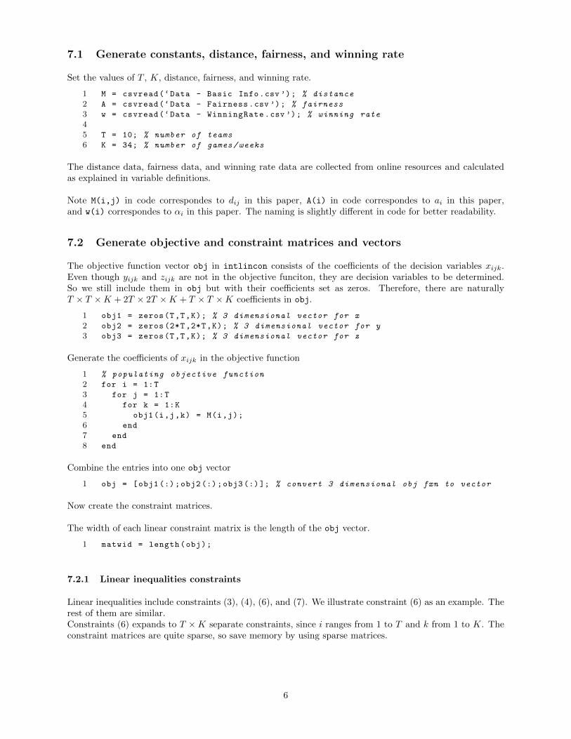
7.2.1 Linear inequalities constraints

Linear inequalities include constraints (3), (4), (6), and (7). We illustrate constraint (6) as an example. Therest of them are similar.Constraints (6) expands to T ×K separate constraints, since i ranges from 1 to T and k from 1 to K. Theconstraint matrices are quite sparse, so save memory by using sparse matrices.

6

1 ...

2 matheight = matheight + T*K % add rows to Aineq&bineq for constraint (6)

3 ... % similarly , add rows for other constraints

45 Aineq = spalloc(matheight , matwid , T*T*K*10); % allocate sparse matrix

6 bineq = zeros(matheight , 1); % allocate bineq as full

78 % Zero matrices of convenient sizes

9 clearer1 = zeros(size(obj1));

10 clearer12 = clearer1 (:);





1516 cnt = 1;

17 % any two teams play at most once additionally

18 for i = 1:T

19 for k = 1:K

20 xtemp = clearer1;

21 % sum xijk over all j as second index

22 xtemp(i, :, k) = xtemp(i, :, k) + 1;

23 % sum xjik over all j as first index

24 xtemp(:, i, k) = xtemp(:, i, k) + 1;

25 % convert to sparse matrix

26 xtemp = sparse ([ xtemp (:); clearer22; clearer32 ]);

27 % fill in the row of Aineq

28 Aineq(cnt , :) = xtemp ’;

29 % fill in the row of bineq

30 bineq(cnt) = 1;

31 cnt = cnt+1;

32 end

33 end

34 ... % similarly , add other linear inequalities constraints

7.2.2 Linear equalities constraints

Linear equalities include constraints (1), (2), (5), and (8) to (11). We illustrate constraint (5) as an example.The rest of them are similar.Constraints (5) expands to T +T separate constraints, since there are two separate parts for home and away,i ranges from 1 to T .

1 ...

2 matheight = matheight + T + T; % add rows to Aineq&bineq for constraint (5)

3 ... % similarly , add rows for other constraints

45 Aeq = spalloc(matheight , matwid , matzeros);

6 beq = zeros(matheight , 1);

78 cnt = 1;

9 % three home games

10 for j = 1:T


12 % sum xijk over all j and k

13 xtemp(:, j, :) = 1;



16 % fill in the row of Aeq

17 Aeq(cnt , :) = xtemp ’;

7

18 % same for beq

19 beq(cnt) = 3;

20 cnt = cnt +1;

21 end

2223 % three away games

24 for i = 1:T


26 % sum xijk over all i and k

27 xtemp(i, :, :) = 1;



30 % fill in the row of Aeq

31 Aeq(cnt , :) = xtemp ’;

32 % same for beq

33 beq(cnt) = 3;

34 cnt = cnt +1;

35 end

36 ... % similarly , add other linear inequalities constraints

7.3 Bound constraints and integer variables

The integer variables are all those from obj.

1 intcon = 1: length(obj);

The upper bounds and lower bounds are for the above set of integer variables also. Upper bounds are allones, and lower bounds are all zeros.

1 lb = zeros(length(obj), 1);

2 ub = zeros(length(obj), 1);

3 ub(:) = 1;

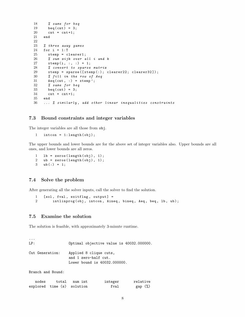
7.4 Solve the problem

After generating all the solver inputs, call the solver to find the solution.

1 [sol , fval , exitflag , output] =

2 intlinprog(obj , intcon , Aineq , bineq , Aeq , beq , lb , ub);

7.5 Examine the solution

The solution is feasible, with approximately 3-minute runtime.

...

LP: Optimal objective value is 40032.000000.

Cut Generation: Applied 8 clique cuts,

and 1 zero-half cut.

Lower bound is 40032.000000.

Branch and Bound:

nodes total num int integer relative

explored time (s) solution fval gap (%)

8

3315 190.34 1 4.003200e+04 0.000000e+00

Optimal solution found.

Intlinprog stopped because the objective value is within a gap tolerance of the

optimal value, options.AbsoluteGapTolerance = 0 (the default value). The intcon

variables are integer within tolerance, options.IntegerTolerance = 1e-05 (the

default value).

To obtain the schedule:

1 % Reshapte the result matrix by x, y, z’s variables vector sizes

2 xs = sol (1: length(clearer12));

3 X = reshape(xs , T, T, K);

45 ... % translate 3 dimensional vector X to print as

6 ... % ‘team i plays with team j on week k’

78 ... % do the same for 3 dimensional vectors Y and Z

The output is the concrete schedule.

8 Results and Comparison

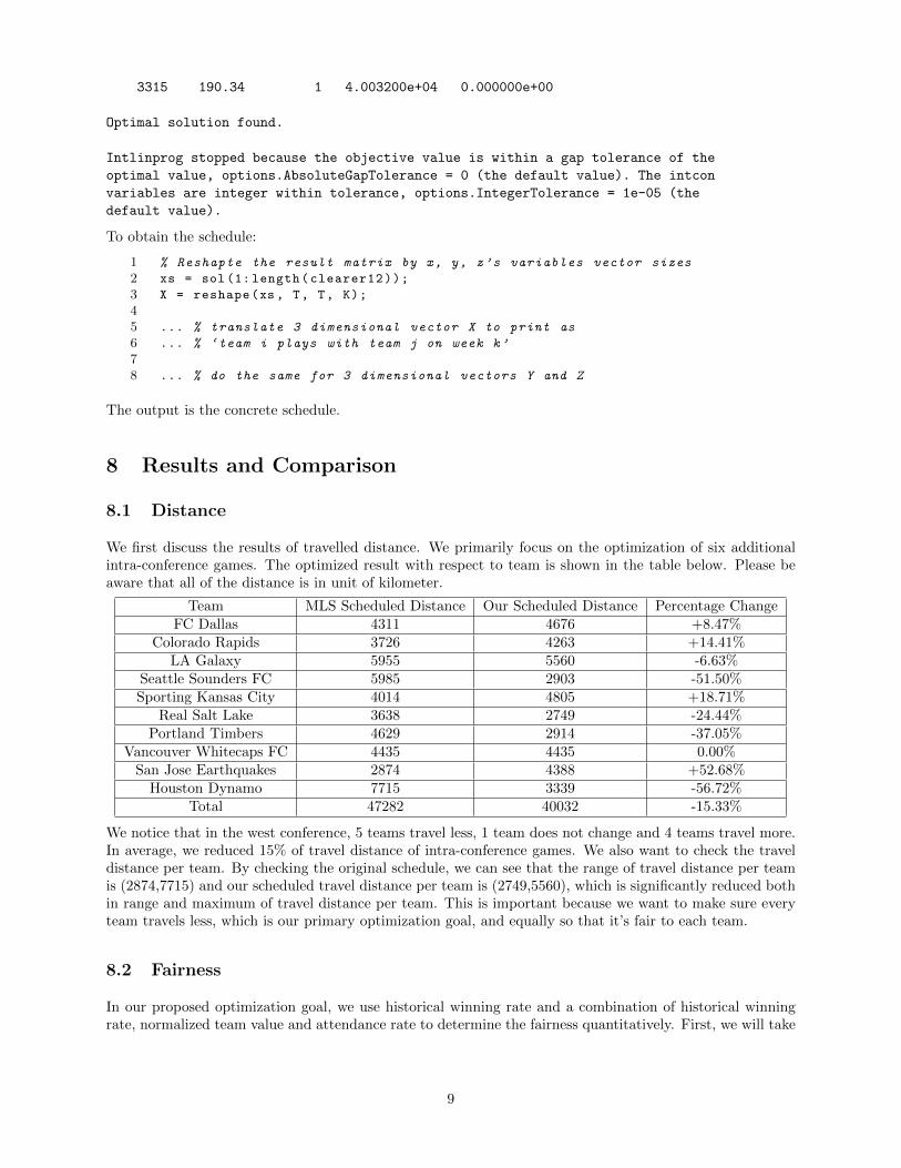
8.1 Distance

We first discuss the results of travelled distance. We primarily focus on the optimization of six additionalintra-conference games. The optimized result with respect to team is shown in the table below. Please beaware that all of the distance is in unit of kilometer.

Team MLS Scheduled Distance Our Scheduled Distance Percentage ChangeFC Dallas 4311 4676 +8.47%

Colorado Rapids 3726 4263 +14.41%LA Galaxy 5955 5560 -6.63%

Seattle Sounders FC 5985 2903 -51.50%Sporting Kansas City 4014 4805 +18.71%

Real Salt Lake 3638 2749 -24.44%Portland Timbers 4629 2914 -37.05%

Vancouver Whitecaps FC 4435 4435 0.00%San Jose Earthquakes 2874 4388 +52.68%

Houston Dynamo 7715 3339 -56.72%Total 47282 40032 -15.33%

We notice that in the west conference, 5 teams travel less, 1 team does not change and 4 teams travel more.In average, we reduced 15% of travel distance of intra-conference games. We also want to check the traveldistance per team. By checking the original schedule, we can see that the range of travel distance per teamis (2874,7715) and our scheduled travel distance per team is (2749,5560), which is significantly reduced bothin range and maximum of travel distance per team. This is important because we want to make sure everyteam travels less, which is our primary optimization goal, and equally so that it’s fair to each team.

8.2 Fairness

In our proposed optimization goal, we use historical winning rate and a combination of historical winningrate, normalized team value and attendance rate to determine the fairness quantitatively. First, we will take

9

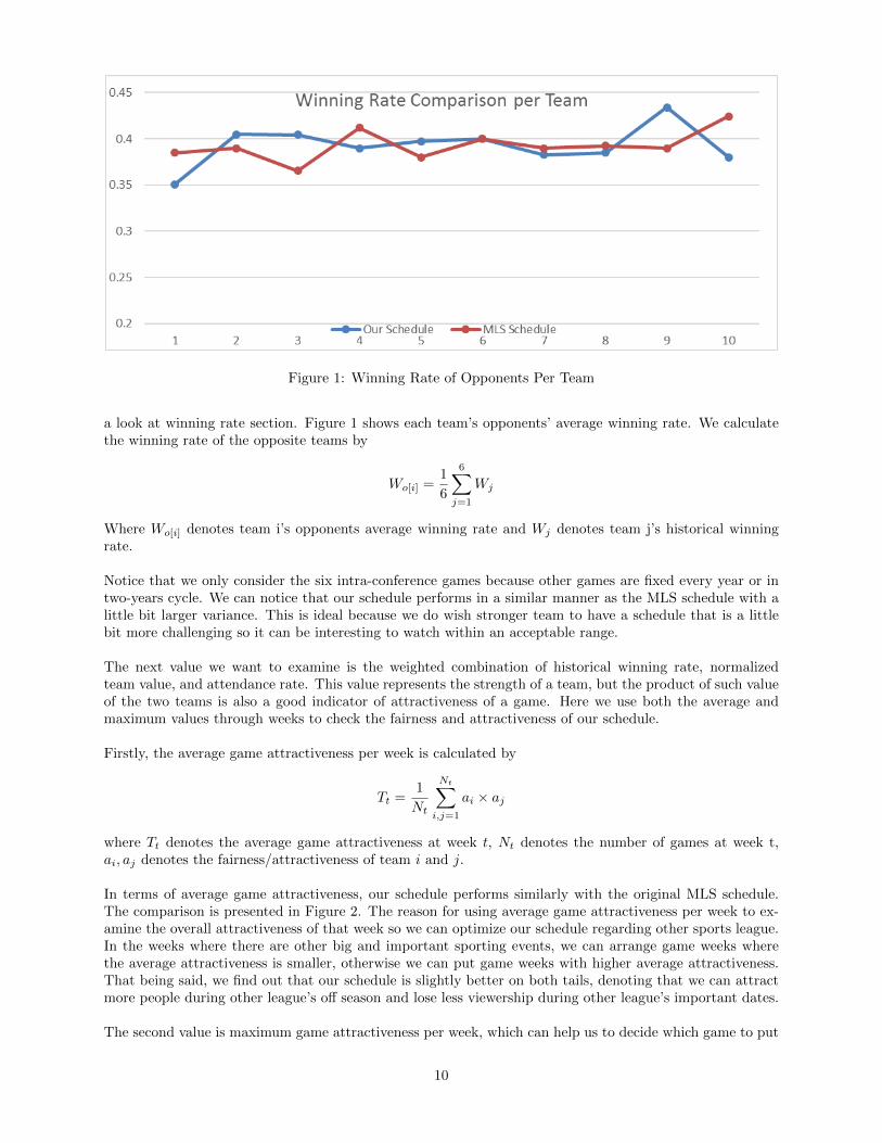
Figure 1: Winning Rate of Opponents Per Team

a look at winning rate section. Figure 1 shows each team’s opponents’ average winning rate. We calculatethe winning rate of the opposite teams by

Wo[i] =1

6

6∑j=1

Wj

Where Wo[i] denotes team i’s opponents average winning rate and Wj denotes team j’s historical winningrate.

Notice that we only consider the six intra-conference games because other games are fixed every year or intwo-years cycle. We can notice that our schedule performs in a similar manner as the MLS schedule with alittle bit larger variance. This is ideal because we do wish stronger team to have a schedule that is a littlebit more challenging so it can be interesting to watch within an acceptable range.

The next value we want to examine is the weighted combination of historical winning rate, normalizedteam value, and attendance rate. This value represents the strength of a team, but the product of such valueof the two teams is also a good indicator of attractiveness of a game. Here we use both the average andmaximum values through weeks to check the fairness and attractiveness of our schedule.

Firstly, the average game attractiveness per week is calculated by

Tt =1

Nt

Nt∑i,j=1

ai × aj

where Tt denotes the average game attractiveness at week t, Nt denotes the number of games at week t,ai, aj denotes the fairness/attractiveness of team i and j.

In terms of average game attractiveness, our schedule performs similarly with the original MLS schedule.The comparison is presented in Figure 2. The reason for using average game attractiveness per week to ex-amine the overall attractiveness of that week so we can optimize our schedule regarding other sports league.In the weeks where there are other big and important sporting events, we can arrange game weeks wherethe average attractiveness is smaller, otherwise we can put game weeks with higher average attractiveness.That being said, we find out that our schedule is slightly better on both tails, denoting that we can attractmore people during other league’s off season and lose less viewership during other league’s important dates.

The second value is maximum game attractiveness per week, which can help us to decide which game to put

10

Figure 2: Average Game Attractiveness Per Week

Figure 3: Average Game Attractiveness Per Week

11

on prime time. The comparison is shown in Figure 3. Again, our schedule performs very similar comparedwith MLS’s original schedule.

9 Discussion

9.1 Robustness

Since the number of teams and weeks are pretty much fixed, the only factors that might influence robustnessare the weights in fairness values. By testing different values, we found out that the weights have minimalinfluence on the final schedule. This influence shows that commercial value, winning rate, and attendancerate are equally important in determining the strength of a team. Therefore we decided to equally distributetheir weights in representing their share of influence in the model.

As for other changing coefficients, which are the upper and lower bounds L, U, and P for fairness andattractiveness, we tested by evaluating final results and finding the tightest bound that gives a feasiblesolution.

9.2 Further Discussion

1. Bye weeks

MLS sometimes have bye weeks, in which a team doesn’t play any game during the whole week.It ensures that players have enough time to rest and extends the length of a regular season for com-mercial reasons. Since most of the bye weeks are determined by various complex factors like nationalteam games and other major sport events, it is very hard to summarize a formulation in this model.But in real life, it is necessary to study the reasons and ways to schedule bye weeks if given enoughdata and resources.

2. Complete schedule

After scheduling for the Western Conference, we can easily apply the same method to the EasternConference as well. Obviously there is no conflict between the 24 infra-conference games, but it isnecessary to consider the 10 cross-conference games. Since crossing the states is a relatively long flight,it might be more efficient to schedule two away games within a week so that the away team doesn’tneed to fly too much. But at the same time we still need to maintain the home-away balance.

10 Conclusion

As many factors may influence a sports scheduling problem, our model simplifies and quantifies major vari-ables like traveling distance, fairness, and attractiveness to achieve an efficient, fair, and interesting gameschedule. The result shows that our model performs equally good with and even better than the officialschedule, specifically in reducing travelling distance, balancing team strength, and enhancing game attrac-tiveness. We tried to consider as many non-quantifiable variables as possible by adapting the programmingoutput to real life cases, but there are still many factors that could be taken into consideration. Fortunately,due to a relatively high robustness, it is repeatable with different conferences or seasons, thus can be testedand subject to changes in future studies.

12

A Final Schedule

The final schedule is obtained by MATLAB output and manually alternating some games by non-quantifiablefactors, like weather and special events. Home away balance and mid-week games are also considered andchecked in this final schedule.

B References

[1] RIBEIRO, CELSO C. SPORTS SCHEDULING: PROBLEMS AND APPLICATIONS. (2011).http://www.dcc.ic.uff.br/˜celso/artigos/sports-scheduling.pdf

[2] NEMHAUSER, G. L. & TRICK, M. A. SCHEDULING A MAJOR COLLEGE BASKETBALL CON-FERENCE. (1997).http://mat.gsia.cmu.edu/trick/acc.pdf

[3] MATHWORKS. Factory, Warehouse, Sales Allocation Modelhttps://www.mathworks.com/help/optim/ug/factory-warehouse-sales-allocation-model.html

13

Major League Soccer Scheduling Problem - CMU · Major League Soccer Scheduling Problem Canto Zhu, Muchen Zhou, Qiuyi Jia, Xiang Luo Dec.16 2016 1 Introduction Major League Soccer

Documents