Chapter 1 Machine Learning Methods for Automatic Image Colorization GUILLAUME C HARPIAT Pulsar Project INRIA Sophia-Antipolis, France Email: [email protected] I LJA B EZRUKOV MATTHIAS HOFMANN Y ASEMIN ALTUN B ERNHARD S CH ¨ OLKOPF Max Planck Institute for Biological Cybernetics T¨ ubingen, Germany Email: [email protected] 1.1 Introduction Automatic image colorization is the task of adding colors to a new grayscale image without any user inter- vention. This problem is ill-posed in the sense that there is not a unique colorization of a grayscale image without any prior knowledge. Indeed, many objects can have different colors. This is not only true for

Welcome message from author
This document is posted to help you gain knowledge. Please leave a comment to let me know what you think about it! Share it to your friends and learn new things together.
Transcript

Chapter 1
Machine Learning Methods for Automatic
Image Colorization
GUILLAUME CHARPIAT
Pulsar ProjectINRIASophia-Antipolis, FranceEmail: [email protected]
ILJA BEZRUKOV
MATTHIAS HOFMANN
YASEMIN ALTUN
BERNHARD SCHOLKOPF
Max Planck Institute for Biological CyberneticsTubingen, GermanyEmail: [email protected]
1.1 Introduction
Automatic image colorization is the task of adding colors to a new grayscale image without any user inter-
vention. This problem is ill-posed in the sense that there is not a unique colorization of a grayscale image
without any prior knowledge. Indeed, many objects can have different colors. This is not only true for
2 Computational Photography: Methods and Applications
artificial objects, such as plastic objects which can have random colors, but also for natural objects such
as tree leaves which can have various nuances of green and brown in different seasons, without significant
change of shape.
The most common color prior in the literature is the user. Most image colorization methods allow the
user to determine the color of some areas and extend this information to the whole image, either by pre-
computing a segmentation of the image into (preferably) homogeneous color regions, or by spreading color
flows from the user-defined color points. The latter approach involves defining a color flow function on
neighboring pixels and typically estimates this as a simple function of local grayscale intensity variations[1,
2, 3], or as a predefined threshold such that color edges are detected[4]. However, this simple and efficient
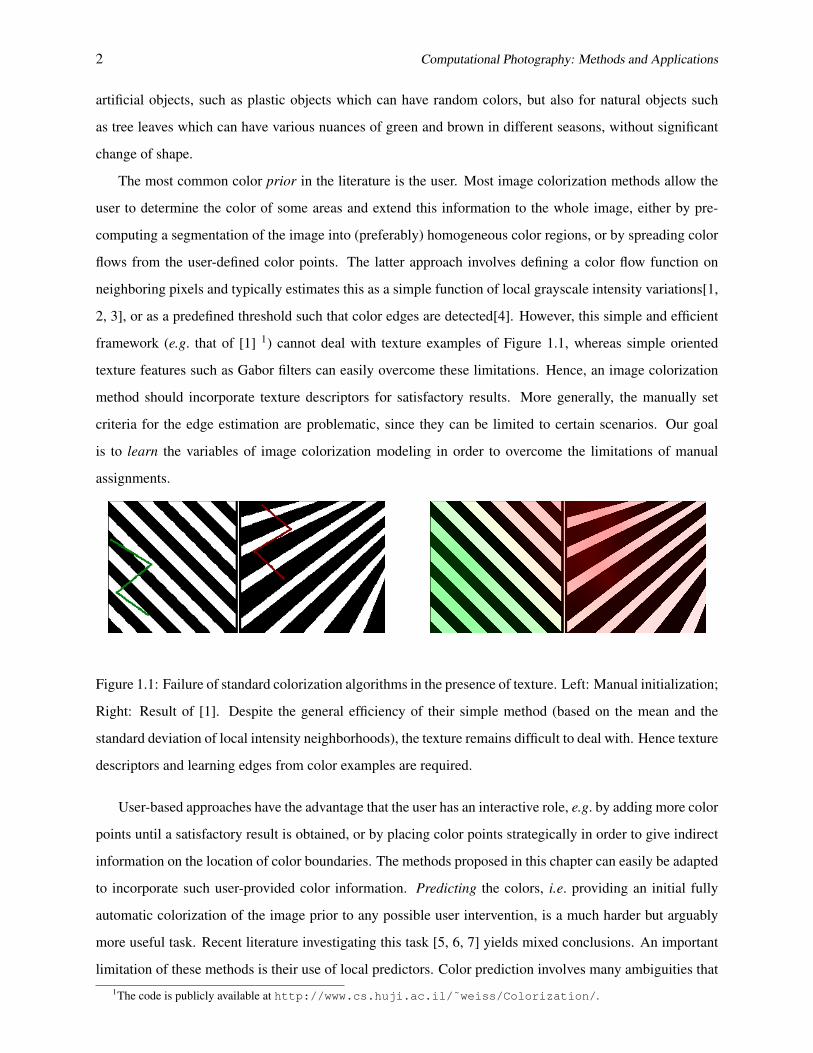
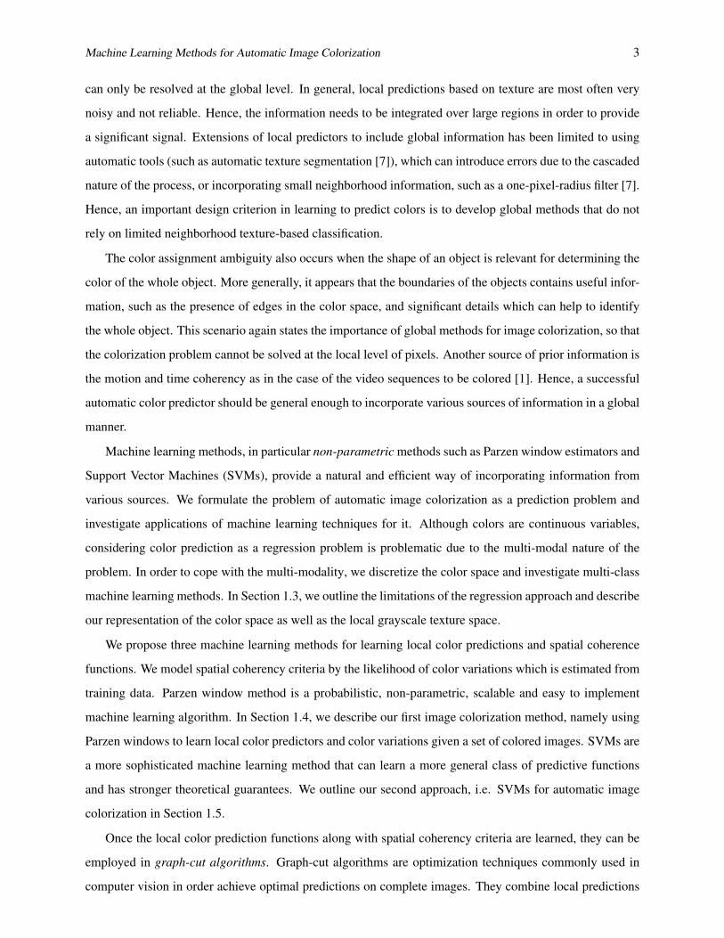
framework (e.g. that of [1] 1) cannot deal with texture examples of Figure 1.1, whereas simple oriented
texture features such as Gabor filters can easily overcome these limitations. Hence, an image colorization
method should incorporate texture descriptors for satisfactory results. More generally, the manually set
criteria for the edge estimation are problematic, since they can be limited to certain scenarios. Our goal
is to learn the variables of image colorization modeling in order to overcome the limitations of manual
assignments.
Figure 1.1: Failure of standard colorization algorithms in the presence of texture. Left: Manual initialization;
Right: Result of [1]. Despite the general efficiency of their simple method (based on the mean and the
standard deviation of local intensity neighborhoods), the texture remains difficult to deal with. Hence texture
descriptors and learning edges from color examples are required.
User-based approaches have the advantage that the user has an interactive role, e.g. by adding more color
points until a satisfactory result is obtained, or by placing color points strategically in order to give indirect
information on the location of color boundaries. The methods proposed in this chapter can easily be adapted
to incorporate such user-provided color information. Predicting the colors, i.e. providing an initial fully
automatic colorization of the image prior to any possible user intervention, is a much harder but arguably
more useful task. Recent literature investigating this task [5, 6, 7] yields mixed conclusions. An important
limitation of these methods is their use of local predictors. Color prediction involves many ambiguities that1The code is publicly available at http://www.cs.huji.ac.il/˜weiss/Colorization/.
Machine Learning Methods for Automatic Image Colorization 3
can only be resolved at the global level. In general, local predictions based on texture are most often very
noisy and not reliable. Hence, the information needs to be integrated over large regions in order to provide
a significant signal. Extensions of local predictors to include global information has been limited to using
automatic tools (such as automatic texture segmentation [7]), which can introduce errors due to the cascaded
nature of the process, or incorporating small neighborhood information, such as a one-pixel-radius filter [7].
Hence, an important design criterion in learning to predict colors is to develop global methods that do not
rely on limited neighborhood texture-based classification.
The color assignment ambiguity also occurs when the shape of an object is relevant for determining the
color of the whole object. More generally, it appears that the boundaries of the objects contains useful infor-
mation, such as the presence of edges in the color space, and significant details which can help to identify
the whole object. This scenario again states the importance of global methods for image colorization, so that
the colorization problem cannot be solved at the local level of pixels. Another source of prior information is
the motion and time coherency as in the case of the video sequences to be colored [1]. Hence, a successful
automatic color predictor should be general enough to incorporate various sources of information in a global
manner.
Machine learning methods, in particular non-parametric methods such as Parzen window estimators and
Support Vector Machines (SVMs), provide a natural and efficient way of incorporating information from
various sources. We formulate the problem of automatic image colorization as a prediction problem and
investigate applications of machine learning techniques for it. Although colors are continuous variables,
considering color prediction as a regression problem is problematic due to the multi-modal nature of the
problem. In order to cope with the multi-modality, we discretize the color space and investigate multi-class
machine learning methods. In Section 1.3, we outline the limitations of the regression approach and describe
our representation of the color space as well as the local grayscale texture space.
We propose three machine learning methods for learning local color predictions and spatial coherence
functions. We model spatial coherency criteria by the likelihood of color variations which is estimated from
training data. Parzen window method is a probabilistic, non-parametric, scalable and easy to implement
machine learning algorithm. In Section 1.4, we describe our first image colorization method, namely using
Parzen windows to learn local color predictors and color variations given a set of colored images. SVMs are
a more sophisticated machine learning method that can learn a more general class of predictive functions
and has stronger theoretical guarantees. We outline our second approach, i.e. SVMs for automatic image
colorization in Section 1.5.
Once the local color prediction functions along with spatial coherency criteria are learned, they can be
employed in graph-cut algorithms. Graph-cut algorithms are optimization techniques commonly used in
computer vision in order achieve optimal predictions on complete images. They combine local predictions

4 Computational Photography: Methods and Applications
with spatial coherency functions across neighboring pixels. This results in global interaction across pixel
colorings and yields the best coloring for a grayscale image with respect to both predictors. The details of
using graph-cuts for image colorization are given in Section 1.6.
One shortcoming of the approaches outlined above is the independent training of the two components,
namely local color predictor and spatial coherency functions. It can be argued that a joint optimization of
these models can find the optimal parameters, whereas independent training may yield sub-optimal models.
Our third approach investigates this issue and uses structured output prediction techniques where the two
models are trained jointly. We provide details of applying Structured SVMs to automatic image colorization
in Section 1.7.
After a brief discussion of related work in Section 1.2, we provide an experimental analysis of the
proposed machine learning methods on datasets of various sizes in Section 1.8. All of our approaches per-
form well with large number of colors and outperform existing methods. We observe that Parzen window
approach provides very natural colorization, especially when trained on small datasets, and perform reason-
ably well on big datasets. On large training data, SVMs and Structured SVMs leverage the information more
efficiently and yield more natural colorization, with more color details, on the expense of longer training
times. Although our experiments focus on colorization of still images, our framework can be readily ex-
tended to movies. We believe our approach has the potential to enrich existing movie colorization methods
that are sub-optimal in the sense that they heavily rely on user input.
1.2 Related Work
Colorization based on examples of color images is also known as color transfer in the literature. We refer
to [8] for a survey of this field.
Pioneer works [5, 6] opened the field of fully automatic colorization. These first results though promising
are mixed, such that they seem to deal with only a few colors. Also, many small artifacts can be observed.
We conjecture that these artifacts are due to the lack of a suitable spatial coherency criterion. Indeed, in
both cases the colorization process is iterative and consists of searching for each pixel, in scan-line order,
the best match in the training set. These approaches are thus not expressed mathematically, in particular it
is not clear whether an energy function is minimized.
Irony et al. [7] propose finding landmark points in the image where a color prediction algorithm reaches
the highest confidence and applying the method presented in [1] as if these points were given by the user.
This approach assumes the existence of a training set of colored images, that is partially segmented by
the user into regions. The new image is automatically segmented into locally homogeneous regions whose
texture is similar to one of the colored regions in the training data, and the colors are transferred. We observe

Machine Learning Methods for Automatic Image Colorization 5
two limitations of this approach, pre-processing step and spatial coherency. The pre-processing step involves
segmentation of images into regions of homogeneous texture either by the user or by automatic segmentation
tools. Given that fully automatic segmentation (based on texture or any other criteria) is known to be a
difficult problem, an automatic image colorization method that does not rely on automatic segmentation,
such as the approaches described in this chapter can be more robust. The method of [7] incorporates spatial
coherency at a local level via a one-pixel-radius filter and automatic segments. Our approach can capture
global spatial coherency via the graph-cut algorithm which assigns the best coloring to the global image.
1.3 Model for colors and grayscale texture
In the image colorization problem, two important quantities to be modeled are the output space, i.e. the color
space, and the input space, i.e. the feature representation of the grayscale images. Let I denote a grayscale
image to be colored, p the location of one particular pixel, and C a colorization of image I . Hence, I and
C are images of the same size and the color of the pixel p, denoted by C(p), is in the standard RGB color
space. Since the grayscale information is already given by I(p), we restrict C(p) such that computing the
grayscale intensity ofC(p) yields I(p). Thus, the dimension of the color space to be explored is intrinsically
two rather than three.
In this section, we present the model chosen for the color space, the limitations of a regression approach
for color prediction, our color space discretization and how to express probability distributions of continuous
valued colors given a discretization. We also describe the feature space used for the description of grayscale
patches.
1.3.1 L-a-b color space
In order to measure the similarity of two colors, we need a metric on the space of colors. This metric is also
employed to associate a saturated color to its corresponding gray level, i.e. the closest unsaturated color.
It is also at the core of the color coherency problem. An object with uniform reflectance shows different
colors in its illuminated and shadowed parts since they have different gray levels. This behavior creates the
need of a definition that is robust against changes of lightness. More precisely, the modeling of the color
space should specify how colors are expected to vary as a function of the gray level and how a dark color is
projected onto the subset of all colors that share a specific brighter gray level.
There are various color models, such as RGB, CMYK, XY Z and L-a-b. Among these, we choose the
latter since its underlying metric has been designed to express color coherency. The psychophysical L-a-b
color space was historically designed such that the Euclidean distance between the coordinates of any colors
in this space approximates to the human perception of distances between colors as accurately as possible.

6 Computational Photography: Methods and Applications
L-a-b space has three coordinates: L expresses the luminance or lightness and is consequently the grayscale
axis. a and b stand for the two orthogonal color axes. The transformation from standard RGB colors to L-a-b
is achieved by applying first the gamma correction, then a linear function in order to obtain the XY Z color
space, and finally a highly non-linear function which is basically a linear combination of the cubic roots of
the coordinates in XY Z. We refer the reader to http://brucelindbloom.com/ or to [9] for more
details on color spaces. In the following, we refer to L and (a, b) by gray level and 2D color respectively.
Since the gray level I(p) of the color C(p) at pixel p is given, we search only for the remaining 2D color,
denoted by ab(p).
1.3.2 Need for multi-modality
In automatic image colorization, we are interested in learning a function that associates the right color for a
pixel p given a local description of grayscale patches centered at p. Since colors are continuous variables,
we can employ regression tools such as Support Vector Regression or Gaussian Process Regression [10] for
image colorization. Unfortunately, a regression approach performs poorly and there is an intuitive explana-
tion for this performance: Many objects with the same or similar local descriptors can have different colors.
For instance, balloons at a fair could be green, red, blue, etc. Even if the task of recognizing a balloon was
easy and we knew that we should use the observed balloon colors to predict the color of a new balloon,
a regression approach would recommend using the average color of the observed balloons, i.e. gray. This
problem is not specific to objects of the same class, but also extends to objects with similar local descriptors.
For example, the local descriptions of grayscale patches of skin and sky are very similar. Hence, a method
trained on images including both objects would recommend purple for skin and sky, without considering
the fact that this average value is never probable. Therefore, an image colorization method requires multi-
modality, i.e. the ability to predict different colors if needed, or more precisely the ability to predict scores
or probability values of every possible color at each pixel.
1.3.3 Discretization of the color space
Due to the multi-modal nature of the color prediction problem, the machine learning methods proposed in
this paper first infer distributions for discrete colors given a pixel and then project the predicted colors to the
continuous color space. We now discuss a discretization of the 2D color space and a projection method for
continuous valued colors.
There are numerous ways of discretization, for instance via K-means. Instead of setting a regular grid in
the color space, we define a discretization adapted to the colors in the training dataset such that each color
bin contains approximately the same number of pixels. Indeed, some zones of the color space are useless

Machine Learning Methods for Automatic Image Colorization 7
Figure 1.2: Examples of color spectra and associated discretizations. For each line, from left to right: color
image; corresponding 2D colors; the location of the observed 2D colors in the ab-plane (a red dot for each
pixel) and the computed discretization in color bins; color bins filled with their average color; continuous
extrapolation: influence zones of each color bin in the ab-plane (each bin is replaced by a Gaussian, whose
center is represented by a black dot; red circles indicate the standard deviation of colors within the color bin,
blue ones are three times larger).
for many real image datasets. Allocating more color bins to zones with higher density allows the models to
have more nuances where it makes statistical sense. Figure 1.2 shows the densities of colors corresponding
to some images, as well as the discretization of the color space into 73 bins resulting from these densities.
To obtain this discretization, we used a polar coordinate system in ab, cut color bins recursively with highest
numbers of points at their average color into 4 parts, and assigned the average color to each bin.
Given the densities in the discrete color space, we express the densities for continuous colors on the
whole ab plane via interpolation. In order to interpolate the information given by each color bin i contin-
uously, we place Gaussian functions on the average color µi, with standard deviation proportional to the
empirical standard deviation σi (see last column of Figure 1.2). The interpolation of the densities d(i) in the
discrete color space to any point x in the ab plane is given by
dG(x) =∑i
1π(ασi)2
e− ‖x−µi‖
2
2(κσi)2 d(i).
We observed that κ ≈ 2 yields successful experimental results. For better performance, it is possible to
employ cross-validation for the optimal κ value for a given training set.
1.3.4 Grayscale patches and features
As discussed in Section 1.1, the gray level of one pixel is not informative for color prediction. Additional
information such as texture and local context is necessary. In order to extract as much information as possible

8 Computational Photography: Methods and Applications
to describe local neighborhoods of pixels in the grayscale image, we compute SURF descriptors [11] at
three different scales for each pixel. This leads to a vector of 192 features per pixel. We apply Principal
Component Analysis (PCA) and keep the first 27 eigenvectors, in order to reduce the number of features and
to condense the relevant information. Furthermore, as supplementary components, we include the pixel gray
level as well as two biologically inspired features: a weighted standard deviation of the intensity in a 5× 5
neighborhood (whose meaning is close to the norm of the gradient), and a smooth version of its Laplacian.
We refer to this 30-dimensional vector, computed at each pixel q, as local description, and denote it by v(q)
or v, when the text uniquely identifies q.
1.4 Parzen Windows for Color Prediction
Given a set of colored images and a new grayscale image I to be colored, the color prediction task is to
extract knowledge from the training set to predict colors C for the new image. We represent this knowledge
in two models, namely a local color predictor and a spatial coherency function. In this section, we outline
how to use Parzen window method in order to learn these models based on the representation described in
Section 1.3.
1.4.1 Learning local color prediction
Multi-modality of color prediction problem creates the need of predicting scores or probability values for all
possible colors at each pixel. This can be accomplished by modeling the conditional probability distribution
of colors knowing the local description of the grayscale patch around the pixel considered. The conditional
probability of the color ci at pixel p given the local description v of its grayscale neighborhood can be
expressed as the fraction, amongst colored examples ej = (wj , c(j)) whose local description wj is similar
to v, of those whose observed color c(j) is in the same color bin Bi. This can be estimated with a Gaussian
Parzen window model
p(ci|v) =( ∑{j : c(j)∈Bi}
k(wj ,v))/∑
j
k(wj ,v), (1.1)
where k(wj ,v) = e−‖wj−v‖2/2σ2is the Gaussian kernel. The best value for the standard deviation σ can
be estimated by cross-validation on the densities. Parzen windows also allow us to express how reliable
the probability estimation is: its confidence depends directly on the density of examples around v, since an
estimation far from the clouds of observed points loses significance. Thus, the confidence on a probability
estimate is given by the density in the feature space,
p(v) ∝∑j
k(wj ,v).

Machine Learning Methods for Automatic Image Colorization 9
Note that both distributions, p(ci|v) and p(v), require computing the similarities k(v,wj) on all pixel
pairs which can be expensive during both training and prediction. For computational efficiency, we approx-
imate them by restricting the sums to K-nearest neighbors of v in the training set with a sufficiently large
K chosen as a function of the σ and estimate the Parzen densities based on these K points. In practice, we
choose K = 500. Thanks to fast nearest neighbor search techniques such as kD-tree2, the time needed to
compute the predictions for all pixels of a 50× 50 image is only 10 seconds (for a training set of hundreds
of thousands of patches) and this scales linearly with the number of test pixels.
1.4.2 Local color variation prediction
Instead of choosing a prior for spatial coherence, based either on detection of edges, or on the Laplacian of
the intensity, or on a pre-estimated complete segmentation, we learn directly how likely it is to observe a
color variation at a pixel knowing the local description of its grayscale neighborhood, based on a training set
of real color images. The technique is similar to the one detailed in the previous section. For each example
wj of a colored patch, we compute the norm gj of the gradient of the 2D color (in the L-a-b space) at the
center of the patch. The expected color variation g(v) at the center of a new grayscale patch v is then given
by
g(v) =
∑j k(wj ,v) gj∑j k(wj ,v)
.
1.5 Support Vector Machines for Color Prediction
The method proposed in Section 1.4 improves over existing image colorization approaches by learning color
variations and local color predictors using the Parzen window method. In Section 1.6, we outline how to
use these estimators in graph-cut algorithm in order to get spatially coherent color predictions. Before we
describe the details of this technique, we propose further improvements over the Parzen window approach,
by employing Support Vector Machines (SVMs) [12] to learn the local color prediction function.
Equation 1.1 describes the Parzen window estimator for the conditional probability of the colors given
a local grayscale description v. A more general expression for the color prediction function is given by
s(ci|v; αi) =∑j
αi(j)k(wj ,v) (1.2)
where the kernel k satisfies ∀v,v′, k(v,v′) = 〈f(v), f(v′)〉 in a certain space of features f(v), embedded
with an inner product 〈·, ·〉 between feature vectors (more details in [10]). In both Equation 1.1 and Equa-
tion 1.2, the expansions for each color ci are linear in the feature space. The decision boundary between
different colors, which tells which color is the most probable, is consequently an hyperplane. The αi can be2We use the TSTOOL package available at http://www.physik3.gwdg.de/tstool/ without particular optimization.

10 Computational Photography: Methods and Applications
considered as a dual representation of the normal vector λi of the hyperplane separating the color ci from
other colors. The estimator in this primal space can then be represented as
s(ci|v; λi) = 〈λi, f(v)〉 . (1.3)
In Parzen window estimator, all α values are non-zero constants. In order to overcome computational
problems, we proposed restricting α parameters of pixels pj that are not in the neighborhood of v to be
0 in Section 1.4. A more sophisticated classification approach is via Support Vector Machines (SVMs),
which differ from Parzen Window estimators in terms of patterns whose α values are active (non-zero)
and in terms of finding the optimal values for these parameters. In particular, SVMs remove the influence
of correctly classified training points that are far from the decision boundary, since they generally do not
improve the performance of the estimator and removing such instances (setting their corresponding α values
to 0) reduces the computational cost during prediction. Hence, the goal in SVMs is to identify the instances
that are close to the boundaries, commonly referred as support vectors, for each class ci and find the optimal
αi. More precisely, the goal is to discriminate the observed color c(j) for each colored pixel ej = (wj , c(j))
from the other colors as much as possible while keeping a sparse representation in the dual space. This can
be achieved by imposing the margin constraints
s(c(j)|wj ; λc(j))− s(ci|wj ; λi) ≥ 1, ∀j,∀ci 6= c(j), (1.4)
where the decision function is given in Equation 1.3. If these constraints are satisfiable, one can find multiple
solutions by simply scaling the parameters. In order to overcome this problem, it is common to search for
parameters that satisfy the constraints with minimal complexity. This can be accomplished by minimizing
the norm of the solution λ. In cases where the constraints cannot be satisfied, one can allow violations
of the constraints by adding slack variables ξj for each colored pixel ej and penalize the violations in the
optimization, where K denotes the trade-off between the loss term and the regularization term [13] :
12
∑i ||λi||2 +K
∑j ξj , s.t. (1.5)
s(c(j)|wj ; λc(j))− s(c|wj ; λc) ≥ 1− ξj , ∀j,∀c 6= c(j)
ξj ≥ 0, ∀j.
If the constraint is satisfied for a pixel ej and a color ci, SVM yields 0 for αi(j). The pixel-color pairs with
non-zero αi(j) are the pixels that are difficult (and hence critical) for the color prediction task. These pairs
are the support vectors and these are the only training data points that appear in Equation 1.2.
The constraint optimization problem of Equation 1.5 can be rewritten as a Quadratic Program (QP)
in terms of the dual parameters αi for all colors c(i). Minimizing this function yields sparse αi, which
we can use in the local color predictor function (Equation 1.2). While training SVMs is more expensive
Machine Learning Methods for Automatic Image Colorization 11
than training Parzen window estimators, often SVMs yield better prediction performance. We refer the
reader to [10] for more details on SVMs. In our experiments, we use libsvm, which is publicly available
at http://www.csie.ntu.edu.tw/˜cjlin/libsvm/. As in the case of Parzen windows, we use a
Gaussian kernel.
1.6 Global Coherency via Graph Cuts
For each pixel of a new grayscale image, we are now able to estimate scores of all possible colors (within a
large finite set of colors due to the discretization of the color space into bins) using the techniques outlined in
Section 1.4 and in Section 1.5. Similarly, we can estimate the probability of a color variation for each pixel.
If the spatial coherency criterion given by the color variation function is incorporated into the color predictor,
the choice of the best color for a pixel is affected by the probability distributions in the neighborhood. Since
all pixels are connected through neighborhoods, it results in a global interaction across all pixels. Hence,
in order to get spatially coherent colorization the solution should be computed globally, since any local
search can yield suboptimal results. Indeed it may happen that, in some regions that are supposed to be
homogeneous, a few different colors may seem to be the most probable ones at a local level, but that the
winning color at the scale of the region is different, because in spite of its only second rank probability at
the local level, it ensures a good probability everywhere in the whole region. On the opposite end of this
spectrum are the cases where a color is selected in a whole homogeneous region because of its very high
probability at a few points with high confidence. The problem is consequently not trivial, and the issue is to
find a global solution. We propose to use local predictors and color variation models in graph cuts in order
to find spatially coherent colorization.
1.6.1 Energy minimized by graph cuts
The graph cut or max flow algorithm is an optimization technique widely used in computer vision [14, 15]
because of its suitability for many image processing problems, its speed and its guarantee to find a good
local optimum. In the multi-label case with α-expansion [16], it can be applied to all energies of the form∑i Vi(xi)+
∑i∼j Di,j(xi, xj) where xi are the unknown variables that take values in a finite setL of labels,
where the Vi are any functions, and where Di,j are any pair-wise interaction terms with the restriction that
each Di,j(·, ·) should be a metric on L. For the swap-move case, the constraints are weaker [17],
Di,j(α, α) +Di,j(β, β) ≤ Di,j(α, β) +Di,j(β, α) (1.6)
for a pair of labels α and β. We formulate the image colorization problem as an optimization problem:∑p
Vp(c(p)) + ρ∑p∼q
|c(p)− c(q)|Labgp,q
, (1.7)

12 Computational Photography: Methods and Applications
where Vp(c(p)) is the cost of choosing color c(p) locally for pixel p (whose neighboring texture is described
by v(p)) and where gp,q = 2(g(v(p))−1 + g(v(q))−1
)−1 is the harmonic mean of the estimated color
variation at pixels p and q. An 8-neighborhood is considered for the interaction term, and p ∼ q denotes
that p and q are neighbors.
The interaction term between pixels penalizes color variation where it is not expected, according to the
variations predicted in the previous paragraph. The hyper-parameter ρ enables a trade-off between local
color scores and spatial coherence score. It can be estimated using cross validation.
We described two methods that yield scores to local color prediction. These methods can be used in
order to define Vp(c(p)). When using Parzen window estimator, we define the local color cost Vp(c(p)) as
Vp(c(p)) = − log(p(v(p)
) )p(c(p)|v(p)
). (1.8)
Then, Vp penalizes colors which are not probable at the local level according to the probability distributions
obtained in section 1.4.1, with respect to the confidence in the predictions.
When using SVMs, we have two options to define Vp(c(p)). Even though SVMs are not probabilistic,
methods exist to convert SVM decision scores to probabilities [18]. Hence, we can replace p(c(p)|v(p))
term in Equation 1.8 with the probabilistic SVM scores and use graph cut algorithm in order to find spatially
coherent colorization. However, since V is not restricted to be a probabilistic function, we also can directly
use Vp(c(p)) as−s(c(p)|v(p)). This way, we do not require to get the additional p(v(p)) estimate in order
to model the confidence of the local predictor. s(c(p)|v(p)) already captures the confidence via the margin
concept and renders the additional (possibly noisy) estimation unnecessary.
We use the graph cut package3 provided by [17]. The solution for a 50 × 50 image and 73 possible
colors is obtained by graph cuts in a fraction of second and is generally satisfactory. The computation time
scales approximately quadratically with the size of the image, which is still fast, and the algorithm performs
well even on significantly down-scaled versions of the image, so that a good initial colorization can still
be given quickly for very large images as well. The computational costs compete with those of the fastest
colorization techniques [19] while achieving more spatial coherency.
1.6.2 Refinement in the continuous color space
Our method so far makes color predictions in the discrete space. In order to refine our predictions in the
continuous color space, we would like to perform some smoothing.
This can be achieved naturally for Parzen window approach. Once the density estimation is achieved
in the discrete space, we interpolate probability distributions p(ci|v(p)) estimated at each pixel p for each
color bin i, to the whole space of colors with the technique described in section 1.3. This renders Vp(c) well
3available at http://vision.middlebury.edu/MRF/code/

Machine Learning Methods for Automatic Image Colorization 13
defined for continuous color values as well. The energy function given in Equation 1.7 can consequently be
minimized in the continuous space of colors. We start from the solution obtained by graph cuts and refine it
with a gradient descent. This refinement step generally does not introduce large changes such as changing
the color of whole regions, but introduces more nuances.
1.7 Structured Support Vector Machines for Color Prediction
The methods we described so far improves over existing image colorization approaches by learning color
variations and the local color predictors separately and combining them via graph-cut algorithm. We now
propose learning the local color predictor and spatial coherence jointly, as opposed to learning them indepen-
dently as described in Section 1.4 and Section 1.5. This can be accomplished by Structured Prediction meth-
ods. In particular, we describe the application of Structured Support Vector Machines (SVM-Struct) [20]
for automatic image colorization. SVM-Struct is a machine learning method designed to predict structured
objects, such as images, where color prediction for each pixel is influenced by the prediction of neighboring
pixels as well as the local input descriptors.
1.7.1 Joint feature functions and joint estimator
The decision function of SVM-Struct is computed with respect to feature functions that are defined over the
joint input-output variables. The feature functions should capture the dependency of a color to the local char-
acteristics of the gray scale image as well as the dependency of a color to the colors of neighboring pixels.
We have already defined the feature functions for local dependencies in Section 1.3.4, these features were
denoted by v. Furthermore, in Section 1.6, we outlined an effective way of capturing color dependencies
across neighboring pixels,
f(c, c′) =∣∣c− c′∣∣
Lab, (1.9)
which are later scaled with respect to the color variations g. It is conceivable that this dependency is more
pronounced for some color pairs than others. In order to allow the model to learn such distinctions in case of
their existence, we define feature functions given in Equation 1.9 and learn a parameter λcc′ for each color
pair c, c′.
The decision function of SVM-Struct can now be defined with respect to v and the f function,
s(C|I) =∑
p〈λC(p),v(p)〉+∑
p∼q λC(p)C(q)f(C(p), C(q)), (1.10)
where C refers to a color assignment for image I and C(p) denotes its restriction to pixel p, hence the color
assigned to the pixel. As in the case of standard SVMs, there is a kernel expansion of the joint predictor

14 Computational Photography: Methods and Applications
given by
s(C|I) =∑
p
∑j αC(p)(j)k(wj ,v(p)) +
∑p∼q λC(p)C(q)f(C(p), C(q)). (1.11)
Let us discuss this estimator with respect to the previously considered functions. Compared to the SVM
based local prediction function given in Equation 1.2, we observe that this estimator is defined over a full
grayscale image I and its possible colorings C as opposed to the SVM case which is defined over an
individual grayscale pixel p and its colorings c. Furthermore, the spatial coherence criteria (the second term
in Equation 1.11) are incorporated directly rather than by two-step approaches we use in Parzen window
and SVM based methods. We can also observe that our joint predictor, Equation 1.11, is simply a variation
of the energy function used in the graph cut algorithm given in Equation 1.7, where different parameters for
spatial coherence can now be estimated by a joint learning process as opposed to learning color variation and
finding λ in the energy via cross-validation. With the additional symmetry constraint λcc′ = λc′c for each
color pair c, c′, the energy function can be optimized using the graph cuts swap move algorithm. Hence,
SVM-Struct provides a more unified approach for learning parameters and removes the necessity of the
hyper-parameter ρ.
1.7.2 Training structured SVMs
Given the joint estimator in Equation 1.11, we now define the learning procedure to estimate optimal param-
eters αi for all colors ci and λcc′ for all color pairs c, c′. The training procedure is similar to SVMs where
the norm of the parameters is minimized with respect to margin constraints. Note that the margin constraints
are now defined on colored images (Ij , Cj) for all images j in the training data,
s(Cj |Ij)− s(C|Ij) ≥ 1− ξj , ∀j,∀C 6= Cj .
As in SVMs, the goal is to separate the observed coloring Cj of an image Ij from all possible colorings
C of I . We can extend this formulation by quantifying the quality of a particular coloring with respect to
the observed coloring of an image. If a coloring C is similar to the observed coloring Cj for the training
image Ij , the model should relax the margin constraints for C and j. In order to employ this idea in our joint
optimization framework, we define a cost function ∆(C,C ′) that measures the distance between C and C ′
and imposes margin constraints with respect to this cost function,
s(Cj |Ij)− s(C|Ij) ≥ ∆(Cj , C)− ξj , ∀j,∀C 6= Cj .
The incorporation of ∆ renders the constraints of colorings similar to Cj essentially ineffective and leads
to more reliable predictions. We define this cost function as the average perceived difference between two

Machine Learning Methods for Automatic Image Colorization 15
colors across all pixels,
∆(C, C) =∑p
||C(p)− C(p)||maxc,c′ ||c− c′||
. (1.12)
The normalization term ensures that the local color differences are between 0 and 1.
There are efficient training algorithms for this optimization [20]. In our experiments, we used the SVM-
Struct implementation by Thorsten Joachims, available at http://svmlight.joachims.org/, with a
Gaussian kernel.
1.8 Experiments
We now present experimental results of our automatic colorization methods on different datasets.
(a) Given Madonna with the yarnwinder as training data, Mona Lisa is colored using Parzen windows. The border is not colored
because of the window size needed for SURF descriptors.
(b) Color variation predicted
(white stands for homogeneity and
black for color edge)
(c) Most probable color at the local
level
(d) 2D color chosen by graph cuts
Figure 1.3: Da Vinci case : coloring a painting given another painting by the same painter. Note that
previous algorithms could not deal with regions such as the neck or the forehead, where blue is the most
probable color at the local level because grayscale skin resembles sky. The surroundings of these regions
and lower-probability colors are decisive for the final color choice.

16 Computational Photography: Methods and Applications
1.8.1 Colorization based on one example
In Figure 1.3, we colored a famous painting by Leonardo Da Vinci using Parzen window method given
another painting of the painter. The two paintings are significantly different and textures are relatively dis-
similar. The prediction of color variation performs well and helps significantly to determine the boundaries
of homogeneous color regions. The multi-modality framework proves extremely useful in areas such as
Mona Lisa’s forehead or neck where the texture of skin can be easily mistaken with the texture of sky at
the local level. Without our global optimization framework, several entire skin regions would be colored
in blue, disregarding the fact that skin color is the second probable colorization for these areas.This makes
sense at the global level since they are surrounded by skin-colored areas, with low probability of edges. We
insist on the fact that the input of previous texture-based approaches is very similar to the “most probable
color” prediction (second line, middle image), whereas we consider the probabilities of all possible colors at
all pixels. This means that given a certain quality of texture descriptors, we handle much more information.
In Figure 1.4, we report the outcome of similar experiments with photographs of landscapes. The effect
of the refinement step can be observed in the sky, where nuances of blue vary more smoothly. SVMs and
SVM-Struct yields only slightly different results, hence the colorizations are not presented.
(a) Landscape example : training image, test image and result.
(b) Color variation predicted; most probable color locally; 2D color chosen by graph cuts; colors obtained after refinement step.
Figure 1.4: Landscape example with Parzen windows. Note that the sky is more homogeneous after the
refinement step, the color gradients in the sky are smoother than when obtained directly by graph cuts.
We compare our Parzen window method with the one by Irony et al., on their own example [7] in Figure
1.5; the task is easier, and results are similar. The boundaries of our color regions fit better to the zebra
contour, as observed in Figure 1.6. However, grass areas near the zebra are colored according to the grass
observed at similar locations around the zebra in the training image, thus creating color halos which are

Machine Learning Methods for Automatic Image Colorization 17
(a) Our result, for Irony et al.’s example (color zebra example, test image, result).
(b) Our predicted 2D colors(c) Irony et al.’s result with the assumption
that this is a binary classification problem.
Figure 1.5: Comparable results with Irony et al. on their own example[7]. Note that this example could
be solved easily without texture consideration, since there is a simple correspondence between gray level
intensity and color. Concerning our result, the color variations in the grass around the zebra can be explained
by the influence of the grass color for similar patches in the training image. We expect this problem to
disappear with a larger training set. The conclusion is that we should not train models using a single,
carefully-chosen training image.
(a) Irony et al.’s result (b) Our result (c) The colors we predicted
Figure 1.6: A zoom on the previous experiment. In Irony et al.’s result, a several pixel wide band of grass
around the zebra’s legs and abdomen are colored as if they were part of the zebra, while in our results the
contour of the zebra matches exactly boundaries of 2D color regions. This difference is due to the fact that
we estimate the location of boundaries through our color variation prediction.

18 Computational Photography: Methods and Applications
visually not completely satisfactory. We expect this bias to disappear with larger training sets since the color
of the background becomes independent of zebra’s presence.
1.8.2 Colorization based on a small set of different images
We next consider a very difficult task: the one of coloring an image from a Charlie Chaplin movie, with
many different objects and textures, such as a brick wall, a door, a dog, a head, hands and a loose suit.
Because of the number of objects and because of their particular arrangement, it is unlikely to find a single
color image with a similar scene that we can use as a training image. Thus we consider a small set of three
different images, each of which shares a partial similarity with the Charlie Chaplin image. The underlying
difficulty is that each training image also contains parts which should not be re-used in this target image.
Figure 1.7 shows the results using Parzen windows. The result is promising considering the training set.
In spite of the difficulty of the task, the prediction of color edges and of homogeneous regions remains
significant. The brick wall, the door, the head and the hands are globally well colored. The large trousers
are not in the training set; the mistakes in the colors of Charlie Chaplin’s dog are probably due to the blue
reflections on the dog in the training image and to the light brown of its head. Dealing with larger training
datasets increases the computation time only logarithmically, during the kD-tree search.
Figure 1.8 shows the results for SVM-based prediction. In the case of SVM colorization, the contours
of Charlie Chaplin and the dog are well recognizable in the color-only image. Face and hands do not
contain non-skin colors, but the abrupt transitions from very pale to warm tones are visually not satisfying.
The coloring of the dog contains a large fraction of skin colors, a fact which could be attributed to a high
textural similarity between these. The large red patch on the door frame is probably caused by a high local
similarity with the background flag in the first training image. Application of the spatial coherency criterion
from equation 1.7 yields a homogeneous coloring, with skin areas being well represented. The coloring of
the dog does not contain the mistakes from figure 1.7, and appears consistent. The door is colored with
regions of multiple, but similar colors, which roughly follow the edges on the background. The interaction
term effectively prevents transitions between colors that are too different, when the local probabilities are
similar. The third row shows a colorization where the interaction weights were learned with SVM-Struct.
The overall result appears less balanced than the previous one, the dog having patches of skin color and the
face consisting of two not very similar color regions. Given the difficulty of the task and the small amount
of training data, the result is presentable, as all interaction weights were learned automatically.

Machine Learning Methods for Automatic Image Colorization 19
(a) Using three training images, a Charlie Chaplin movie frame is colored.
(b) Prediction of color variations (c) Most probable color at the lo-
cal level
(d) Final result
Figure 1.7: Charlie Chaplin frame colored using Parzen windows with three training images. This example
is particularly difficult because many different textures and colors are involved and because there are not
any color images very similar to the Charlie Chaplin image. We have chosen three training images, each
of which shares a partial similarity with the target image. In spite of the complexity of the problem, the
prediction of color edges and of homogeneous regions remains significant. The brick wall, the door, the
head and the hands are globally well colored. The large trousers are not in the training set; the mistakes in
the colors of Charlie Chaplin’s dog are probably due to the blue reflections on the dog in the training image
and to the light brown of its head. Both can benefit from larger training sets.
(a) SVM (b) SVM with spatial regularization
(equation 1.7)
(c) SVM-Struct
Figure 1.8: Charlie Chaplin frame colored via SVM and SVM-Struct, with the training set of figure 1.7.

20 Computational Photography: Methods and Applications
Figure 1.9: We performed experiments on the Caltech Pasadena Houses 2000 collection, available at
http://www.vision.caltech.edu/archive.html, reproduced with permission. Our training set
consists of the 20 first images of this house database. We show here 8 of these 20 images, the whole set can
be seen at http://www-sop.inria.fr/members/Guillaume.Charpiat/color/houses.html.
(a) 21st image colored (b) 22nd image colored
(c) Predicted edges (21st and 22nd images, re-
spectively)
(d) Most probable color at the pixel level (e) Colors chosen
Figure 1.10: Colorization results on the 21st and 22nd images from the Pasadena houses Caltech dataset.

Machine Learning Methods for Automatic Image Colorization 21
1.8.3 Scaling with training set size
We performed larger-scale experiments on two datasets. The first dataset is based on the first 20 images
of the Pasadena houses Caltech database (Figure 1.9). We use this training data to predict colors for the
21st and 22nd images. Figure 1.10 illustrates colorization using Parzen windows. The colorization quality
is relatively similar to the one obtained for the previous small datasets. In order to remove texture noise
(for example the unexpected red dots in trees in figure 1.10), a higher spatial coherency weight is required,
which explains the lack of nuances. The use of more discriminative texture features can improve texture
identification, reduce texture noise and consequently allow more nuances.
Images colored using SVMs and SVM-Struct are shown in figure 1.11. In order to reduce the training
time, we used every 3rd pixel on a regular grid for all training images.
The shapes of the windows, doors and stairs can be identified from the color-only image, which is not
(a) SVM (21st image) (b) SVM + spatial regularization (21st) (c) SVM-Struct (21st)
(d) SVM (22nd image) (e) SVM + spatial regularization (22nd) (f) SVM-Struct (22nd)
Figure 1.11: Colorization results on the 21st and 22nd images from the Pasadena houses Caltech dataset
using SVM, SVM with spatial regularization, and SVM-Struct (results and colors chosen are displayed).

22 Computational Photography: Methods and Applications
the case for the Parzen window method, demonstrating the ability of SVM to discriminate between fine
details on local level. The colorization of the lawn is irregular, the local predictor tends to switch between
green and gray, which would correspond to a decision between grass or asphalt. This effect does not occur
in the Parzen window classifier and can be attributed to the sub-sampling of the training data, leading to
a comparatively low number of training points for lawn areas. Application of spatial regularization indeed
leads to the effect of the lawn becoming completely gray. When the spatial coherency criterion from equation
1.7, is applied, the coloring becomes homogeneous, and is comparable to the results from the Parzen window
method, but with a higher number of different color regions and thus a more realistic appearance. SVM-
Struct based colorization preserves a much higher number of different color regions while removing most of
the inconsistent color patches and keeping finer details. It is being able to realistically color the small bushes
in front of the second house. The spatial coherency weights for transitions between different colors were
learned from training data without the need for cross validation for the adjustment of the hyper-parameter λ.
These improvements come with expense of longer training time, which scales quadratically with the training
data.
Finally, we performed an ambitious experiment to evaluate how our approach deals with quantities of
different textures on similar objects, i.e. how it scales with the number of textures observed. We built a
portrait database of 53 paintings with very different styles (Figure 1.12), and colored five other portraits
using Parzen windows (Figure 1.13) together with the same parameters. Although given that red color
is indeed the dominant color in an important proportion of the training set, the colorizations sometimes
appear rather reddish.. The surprising part is the good quality of the prediction of the colored edges (last
Figure 1.12: Some of the 53 portraits used as a training set. Styles of paintings are very varied, with
different kinds of textures and different ways of representing edges. The full training set is available at
http://www-sop.inria.fr/members/Guillaume.Charpiat/color/.

Machine Learning Methods for Automatic Image Colorization 23
row of Figure 1.13), which yields a segmentation of the test images into homogeneous color regions. The
boundaries of skin areas in particular are very well estimated, even in the Van Gogh portrait (the fourth
image) which is very heavily textured. The good estimation of color edges helped the colorization process
to find suitable colors inside the supposedly-homogeneous areas, despite locally noisy color predictions. We
did not evaluate SVM and SVM-Struct due to expensive training.
Figure 1.13: The five portraits colored. Top : result. Middle : colors chosen, without grayscale intensity.
Bottom : color edges predicted. These color variations predicted are particularly meaningful and correspond
precisely to the boundaries of the principal regions. Thus, the color edge estimator can be seen as a segmen-
tation tool. The background colors cannot be expected to be correct since the database focuses on faces, for
example the sky in Mona Lisa’s example is not blue because only one blue sky is observed amongst the 53
training portraits. The same parameters were used in the 5 cases.

24 Computational Photography: Methods and Applications
1.9 Discussion
We presented three machine learning methods for automatic image colorization. These methods do not
require any intervention by the user other than the choice of relatively similar training data. We state the
color prediction task formally as an optimization problem with respect to an energy function. Since our
approaches retain the multi-modality until the prediction step, they extract information from training data
effectively using different machine learning methods. The fact that the problem is solved directly at the
global level with the help of graph cuts renders our framework more robust to noise and local prediction
errors. It also makes it possible to resolve large scale ambiguities as opposed to previous approaches. The
multi-modality framework is not specific to image colorization and could be used in any prediction task on
images. For example, [21] outlines a similar approach for medical imaging to predict computed tomography
scans for patients whose magnetic resonance scans are known.
Our framework exploits features derived from various sources of information. It provides a principled
way of learning local color predictors along with spatial coherence criteria as opposed to the previous meth-
ods which chose the spatial coherence criteria manually. Experimental results on small and large scale
experiments demonstrate the validity of our approach which then furthermore shows significant improve-
ments over [5] and [6], in terms of the spatial coherency formulation and the large number of possible colors.
It requires less or similar user-intervention than [7], and can handle cases which are more ambiguous or with
more texture noise.
We would like to emphasize that the automatic colorization results should not be compared to those
obtained by user-interactive approaches since such decisive information is currently not employed in our
method. However, our framework can easily incorporate user-provided information such as the color c
at pixel p in order to modify a colorization that has been obtained automatically. This can be achieved
by clamping the local prediction to the color provided by the user with high confidence. For example, in
Parzen window method, we set p(c|v(p)) = 1 and set the confidence p(v(p)) to a very large value. Similar
clamping assignments are possible for SVM based approaches. Consequently, our optimization framework
is usable for further interactive colorization. A re-colorization with user-provided color landmarks does not
require the re-estimation of color probabilities, and therefore requires only a fraction of second. We leave
this interactive setting as future work.
Acknowledgments
We would like to thank Jason Farquhar, Peter Gehler, Matthew Blaschko and Christoph Lampert for very
fruitful discussions.

Bibliography
[1] A. Levin, D. Lischinski, and Y. Weiss, “Colorization using optimization,” in SIGGRAPH ’04, (Los Angeles,
California), pp. 689–694, ACM Press, August 2004.
[2] L. Yatziv and G. Sapiro, “Fast image and video colorization using chrominance blending,” IEEE Transactions
on Image Processing, vol. 15, pp. 1120–1129, May 2006.
[3] T. Horiuchi, “Colorization algorithm using probabilistic relaxation,” Image Vision Computing, vol. 22, pp. 197–
202, March 2004.
[4] T. Takahama, T. Horiuchi, and H. Kotera, “Improvement on colorization accuracy by partitioning algorithm in
cielab color space,” in Advances in Multimedia Information Processing - PCM 2004, 5th Pacific Rim Conference
on Multimedia (K. Aizawa, Y. Nakamura, and S. Satoh, eds.), vol. 3332 of Lecture Notes in Computer Science,
(Tokyo, Japan), pp. 794–801, Springer, November 2004.
[5] T. Welsh, M. Ashikhmin, and K. Mueller, “Transferring color to greyscale images,” in SIGGRAPH ’02: Proc.
of the 29th annual conf. on Computer graphics and interactive techniques, (San Antonio, Texas), pp. 277–280,
ACM Press, July 2002.
[6] A. Hertzmann, C. E. Jacobs, N. Oliver, B. Curless, and D. H. Salesin, “Image analogies,” in SIGGRAPH 2001,
Computer Graphics Proceedings (E. Fiume, ed.), (Los Angeles, California), pp. 327–340, ACM Press, August
2001.
[7] R. Irony, D. Cohen-Or, and D. Lischinski, “Colorization by Example,” in Proceedings of Eurographics Sym-
posium on Rendering 2005 (EGSR’05, June 29–July 1, 2005, Konstanz, Germany), pp. 201–210, Eurographics
Association 2005, 2005.
[8] F. Pitie, A. Kokaram, and R. Dahyot, “Enhancement of digital photographs using color transfer techniques,” in
Single-Sensor Imaging: Methods and Applications for Digital Cameras (R. Lukac, ed.), ch. 11, pp. 295–321,
CRC Press Image Processing Series, 2008.
[9] R. W. G. Hunt, The Reproduction of Colour. John Wiley, 2004.
[10] B. Scholkopf and A. J. Smola, Learning with Kernels: Support Vector Machines, Regularization, Optimization,
and Beyond. Cambridge, MA, USA: MIT Press, 2001.
[11] H. Bay, T. Tuytelaars, and L. Van Gool, “Surf: Speeded up robust features,” in 9th European Conference on
Computer Vision, (Graz, Austria), May 2006.
25

26 Computational Photography: Methods and Applications
[12] V. Vapnik, Statistical Learning Theory. Wiley-Interscience, 1998.
[13] J. Weston and C. Watkins, “Support vector machines for multi-class pattern recognition,” in Proceedings Euro-
pean Symposium on Artificial Neural Networks, (Bruges, Belgium), April 1999.
[14] Y. Boykov and V. Kolmogorov, “An experimental comparison of min-cut/max-flow algorithms for energy min-
imization in vision,” in EMMCVPR ’01: Proc. of the Third Intl. Workshop on Energy Minimization Methods in
Computer Vision and Pattern Recognition, (London, UK), pp. 359–374, Springer-Verlag, September 2001.
[15] V. Kolmogorov and R. Zabih, “What energy functions can be minimized via graph cuts?,” in European Confer-
ence on Computer Vision, (Copenhagen, Denmark), pp. 65–81, May 2002.
[16] Y. Boykov, O. Veksler, and R. Zabih, “Fast approximate energy minimization via graph cuts,” in International
Conference on Computer Vision, (Kerkyra, Greece), pp. 377–384, September 1999.
[17] R. Szeliski, R. Zabih, D. Scharstein, O. Veksler, V. Kolmogorov, A. Agarwala, M. F. Tappen, and C. Rother,
“A comparative study of energy minimization methods for markov random fields,” in ECCV (2), 9th European
Conference on Computer Vision, Proceedings, Part II (A. Leonardis, H. Bischof, and A. Pinz, eds.), vol. 3952 of
Lecture Notes in Computer Science, (Graz, Austria), pp. 16–29, Springer, May 2006.
[18] J. Platt, “Probabilistic outputs for support vector machines and comparisons to regularized likelihood methods,”
in Advances in Large Margin Classifiers (P. B. Alexander J. Smola, ed.), pp. 61–74, MIT Press, 1999.
[19] G. Blasi and D.-R. Recupero, “Fast Colorization of Gray Images,” in Proc. of Eurographics Italian Chapter,
(Milano, Italy), September 2003.
[20] I. Tsochantaridis, T. Hofmann, T. Joachims, and Y. Altun, “Support vector machine learning for interdependent
and structured output spaces,” in Proceedings of ICML ’04: Twenty-first international conference on Machine
learning, (Banf, Alberta, Canada), July 2004.
[21] M. Hofmann, F. Steinke, V. Scheel, G. Charpiat, J. Farquhar, P. Aschoff, M. Brady, B. Scholkopf, and B. J.
Pichler, “MR-based attenuation correction for PET/MR: A novel approach combining pattern recognition and
atlas registration,” Journal of Nuclear Medicine, November 2008.

Index
L-a-b color space, 5
ambiguity, 2
automatic colorization, 1, 4
automatic image colorization, 1
Charlie Chaplin, 18
color coherency, 5
color edges, 3
color prediction, 3, 8
color space, 3, 5
color space discretization, 6
color transfer, 4
color variation likelihood, 3
color variation prediction, 9
colorization, 1
complexity, 21
conditional probability, 8
confidence, 8
density estimation, 7, 8
dual space, 10
feature space, 9
Gaussian kernel, 8
Gaussian Parzen window, 8
graph cut, 3, 11
image colorization, 1
interactive colorization, 2
L-a-b color space, 5
landscapes, 16
local color prediction, 8, 9
machine learning methods, 3
margin, 10, 14
max flow algorithm, 11
Mona Lisa, 16
multi-class learning, 3
multi-labeling problem, 11
multi-modality, 3, 6, 8
painting style, 22
paintings, 22
Parzen window, 3, 8
portraits, 22
regression, 6
RGB color space, 5
separating hyperplane, 10
spatial coherence, 3, 8, 11, 13
structured output prediction, 4
structured prediction, 13
Structured Support Vector Machines, 13
structured SVM, 4, 13
support vector, 10
Support Vector Machine, 3, 9
SURF features, 8
SVM, 3, 9
SVM-Struct, 13
texture features, 2
zebra, 16
27
Related Documents