Machine Learning: Basis and Wavelet Haar DWT in 2 levels 7 22 38 191 17 83 188 211 71 167 194 207 159 187 201 216 -20 -44 -31 -7 135 -40 -17 -46 13 -32 -17 1 -18 -42 -27 -4 32 157 146 204 김 화 평 (CSE ) Medical Image computing lab 서진근교수 연구실 + + - - + - + - + - - + + + + +

Welcome message from author
This document is posted to help you gain knowledge. Please leave a comment to let me know what you think about it! Share it to your friends and learn new things together.
Transcript

Machine Learning: Basis and Wavelet
Haar DWT in 2 levels
𝒇𝒇
7 22 38 191
17 83 188 211
71 167 194 207
159 187 201 216
-20 -44
-31 -7
135
-40 -17
-46
13 -32
-17 1
-18 -42
-27 -4
32 157
146 204
김 화 평 (CSE ) Medical Image computing lab 서진근교수 연구실
+ +
- -
+ -
+ -
+ -
- +
+ +
+ +
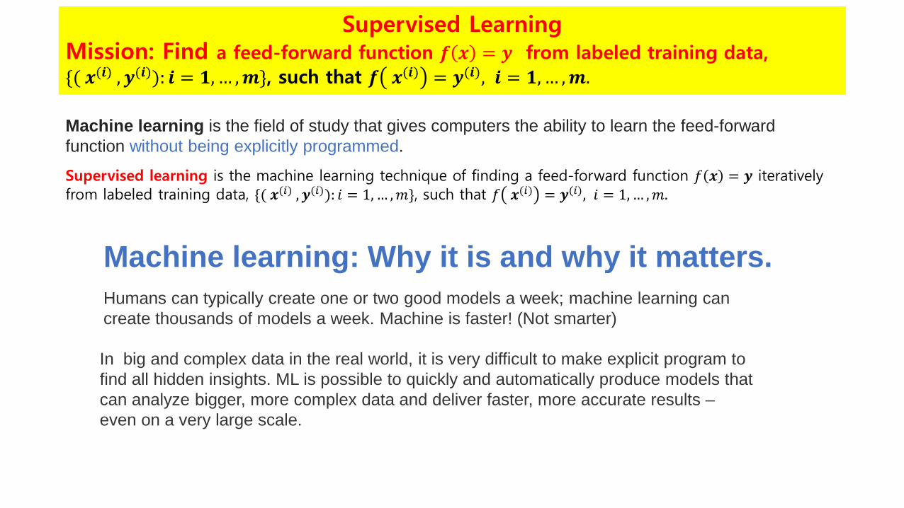
Machine learning is the field of study that gives computers the ability to learn the feed-forward function without being explicitly programmed.
Supervised Learning Mission: Find a feed-forward function 𝒇𝒇 𝒙𝒙 = 𝒚𝒚 from labeled training data, {( 𝒙𝒙
(𝒊𝒊) ,𝒚𝒚
(𝒊𝒊)): 𝒊𝒊 = 𝟏𝟏, … ,𝒎𝒎}, such that 𝒇𝒇 𝒙𝒙 (𝒊𝒊) = 𝒚𝒚
(𝒊𝒊), 𝒊𝒊 = 𝟏𝟏, … ,𝒎𝒎.
Supervised learning is the machine learning technique of finding a feed-forward function 𝑓𝑓 𝒙𝒙 = 𝒚𝒚 iteratively from labeled training data, {( 𝒙𝒙
(𝑖𝑖) ,𝒚𝒚
(𝑖𝑖)): 𝑖𝑖 = 1, … ,𝑚𝑚}, such that 𝑓𝑓 𝒙𝒙 (𝑖𝑖) = 𝒚𝒚
(𝑖𝑖), 𝑖𝑖 = 1, … ,𝑚𝑚.
Machine learning: Why it is and why it matters. Humans can typically create one or two good models a week; machine learning can create thousands of models a week. Machine is faster! (Not smarter)
In big and complex data in the real world, it is very difficult to make explicit program to find all hidden insights. ML is possible to quickly and automatically produce models that can analyze bigger, more complex data and deliver faster, more accurate results – even on a very large scale.
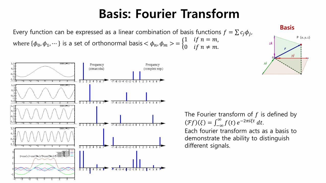
Basis: Fourier Transform Basis
The Fourier transform of 𝑓𝑓 is defined by ℱ𝑓𝑓 𝜉𝜉 = ∫ 𝑓𝑓(𝑡𝑡)∞
−∞ 𝑒𝑒−2𝜋𝜋𝑖𝑖𝜋𝜋𝜋𝜋 𝑑𝑑𝑡𝑡. Each fourier transform acts as a basis to demonstrate the ability to distinguish different signals.
Every function can be expressed as a linear combination of basis functions 𝑓𝑓 = ∑𝑐𝑐𝑗𝑗𝜙𝜙𝑗𝑗,
where 𝜙𝜙0,𝜙𝜙1,⋯ is a set of orthonormal basis < 𝜙𝜙𝑛𝑛,𝜙𝜙𝑚𝑚 > = �1 𝑖𝑖𝑓𝑓 𝑛𝑛 = 𝑚𝑚,0 𝑖𝑖𝑓𝑓 𝑛𝑛 ≠ 𝑚𝑚.

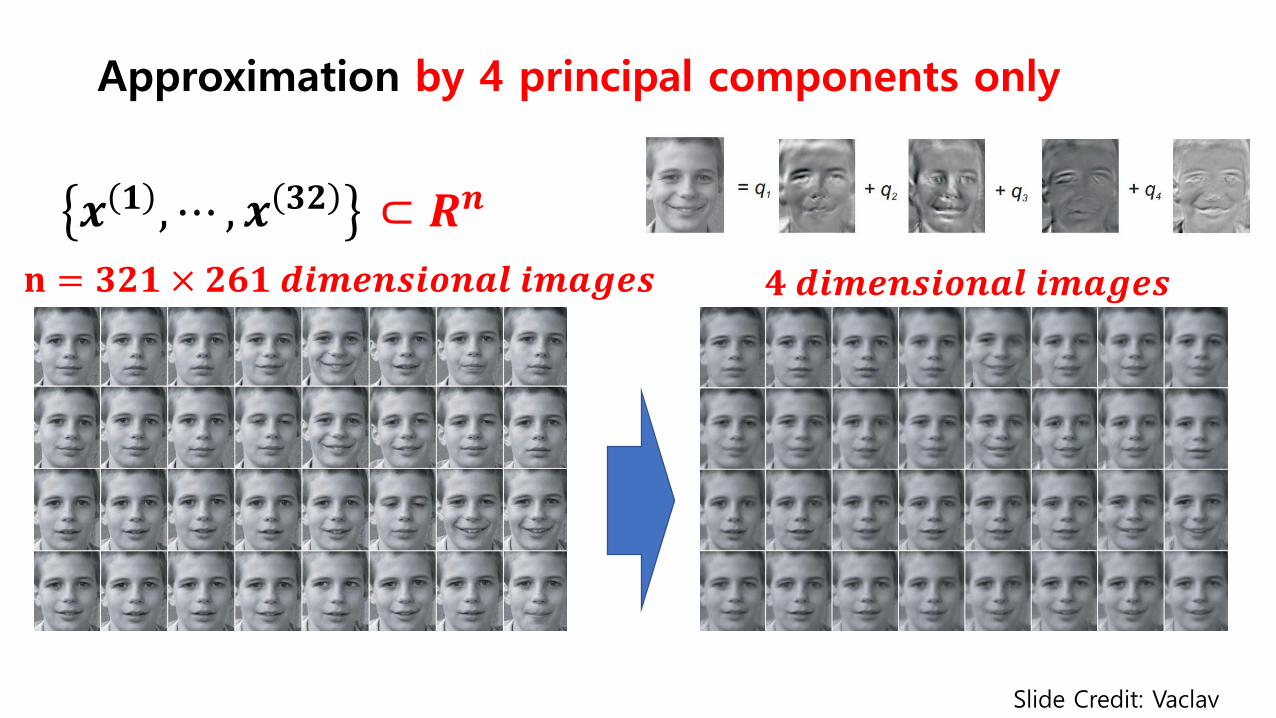
Approximation by 4 principal components (basis) only
𝒙𝒙 𝟏𝟏 ,⋯ ,𝒙𝒙 𝟑𝟑𝟑𝟑 ⊂ 𝑹𝑹𝒏𝒏 𝐧𝐧 = 𝟑𝟑𝟑𝟑𝟏𝟏 × 𝟑𝟑𝟐𝟐𝟏𝟏 𝒅𝒅𝒊𝒊𝒎𝒎𝒅𝒅𝒏𝒏𝒅𝒅𝒊𝒊𝒅𝒅𝒏𝒏𝒅𝒅𝒅𝒅 𝒊𝒊𝒎𝒎𝒅𝒅𝒊𝒊𝒅𝒅𝒅𝒅 𝟒𝟒 𝒅𝒅𝒊𝒊𝒎𝒎𝒅𝒅𝒏𝒏𝒅𝒅𝒊𝒊𝒅𝒅𝒏𝒏𝒅𝒅𝒅𝒅 𝒊𝒊𝒎𝒎𝒅𝒅𝒊𝒊𝒅𝒅𝒅𝒅
Slide Credit: Vaclav
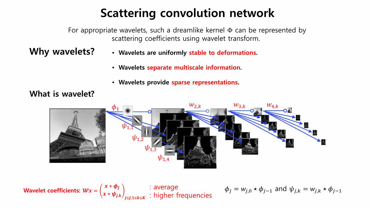
𝜙𝜙𝑗𝑗 = 𝑤𝑤𝑗𝑗,0 ⋆ 𝜙𝜙𝑗𝑗−1 and 𝜓𝜓𝑗𝑗,𝑘𝑘 = 𝑤𝑤𝑗𝑗,𝑘𝑘 ⋆ 𝜙𝜙𝑗𝑗−1 Wavelet coefficients: 𝓦𝓦𝒙𝒙 =𝒙𝒙 ⋆ 𝝓𝝓𝑱𝑱𝒙𝒙 ⋆ 𝝍𝝍𝒋𝒋,𝒌𝒌 𝒋𝒋≤𝑱𝑱,𝟏𝟏≤𝒌𝒌≤𝑲𝑲
: average : higher frequencies
𝑤𝑤2,𝑘𝑘 𝑤𝑤3,𝑘𝑘 𝑤𝑤4,𝑘𝑘 𝜙𝜙1
𝜓𝜓1,1
𝜓𝜓1,2 𝜓𝜓1,3
𝜓𝜓1,4
What is wavelet?
Why wavelets? • Wavelets are uniformly stable to deformations.
• Wavelets separate multiscale information.
• Wavelets provide sparse representations.
Scattering convolution network For appropriate wavelets, such a dreamlike kernel Φ can be represented by
scattering coefficients using wavelet transform.
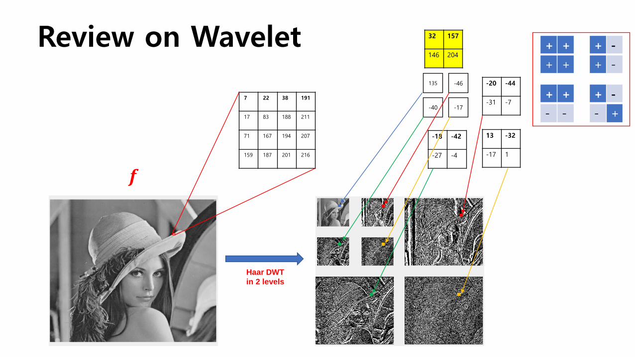
Review on Wavelet
Haar DWT in 2 levels
𝒇𝒇
7 22 38 191
17 83 188 211
71 167 194 207
159 187 201 216
-20 -44
-31 -7
135
-40 -17
-46
13 -32
-17 1
-18 -42
-27 -4
32 157
146 204
+ +
- -
+ -
+ -
+ -
- +
+ +
+ +

𝝍𝝍𝒋𝒋,𝒌𝒌 𝒙𝒙 ≔ 𝟑𝟑𝒋𝒋/𝟑𝟑𝝍𝝍(𝟑𝟑𝒋𝒋𝒙𝒙 − 𝒌𝒌) for 𝟎𝟎 ≤ 𝒌𝒌 < 𝟑𝟑𝒋𝒋.
Wavelet basis functions: The family of functions {𝝍𝝍𝒋𝒋,𝒌𝒌: 𝒋𝒋,𝒌𝒌 ∈ ℤ}, dyadic translations and dilations of a mother wavelet function 𝝍𝝍, construct a complete orthonormal Hilbert basis.
= 𝒇𝒇 𝒙𝒙 = 𝒄𝒄𝝓𝝓 𝒙𝒙 + � � 𝒄𝒄𝒋𝒋,𝒌𝒌𝝍𝝍𝒋𝒋,𝒌𝒌(𝒙𝒙)𝟑𝟑𝒋𝒋−𝟏𝟏
𝒌𝒌=𝟎𝟎
𝟑𝟑
𝒋𝒋=𝟎𝟎
where 𝒄𝒄 = ∫ 𝒇𝒇(𝒙𝒙)∞−∞ 𝝓𝝓 𝒙𝒙 𝒅𝒅𝒙𝒙,
𝒄𝒄𝒋𝒋,𝒌𝒌 = � 𝒇𝒇(𝒙𝒙)∞
−∞𝝍𝝍𝒋𝒋,𝒌𝒌 𝒙𝒙 𝒅𝒅𝒙𝒙.
𝜓𝜓0,0(𝑥𝑥) = 𝜓𝜓(𝑥𝑥)
𝜓𝜓1,0(𝑥𝑥) = 21/2𝜓𝜓(2𝑥𝑥) 𝜓𝜓1,1(𝑥𝑥) = 21/2𝜓𝜓(2𝑥𝑥 − 1)
𝜓𝜓2,1(𝑥𝑥) = 2 𝜓𝜓(22𝑥𝑥 − 1) 𝜓𝜓2,2(𝑥𝑥) = 2𝜓𝜓(22𝑥𝑥 − 2) 𝜓𝜓2,3(𝑥𝑥) = 2 𝜓𝜓(22𝑥𝑥 − 3) 𝜓𝜓2,4(𝑥𝑥) = 2 𝜓𝜓(22𝑥𝑥 − 4)
𝜙𝜙(𝑥𝑥)
Discrete Haar wavelet Transform
𝒇𝒇(𝒙𝒙)

=
+ 𝟎𝟎 ×
+ 𝟑𝟑 ×
+ 𝟏𝟏 ×
+ 𝟑𝟑 ×
− 𝟏𝟏 × − 𝟑𝟑 × − 𝟑𝟑 ×
𝟐𝟐 ×
Approximate the signal from wavelet coefficients
𝒇𝒇 𝒙𝒙 ≈ 𝒄𝒄𝝓𝝓 𝒙𝒙 + � � 𝒄𝒄𝒋𝒋,𝒌𝒌𝝍𝝍𝒋𝒋,𝒌𝒌(𝒙𝒙)𝟑𝟑𝒋𝒋−𝟏𝟏
𝒌𝒌=𝟎𝟎
𝟑𝟑
𝒋𝒋=𝟎𝟎
𝒄𝒄 = 𝟐𝟐 = � 𝒇𝒇(𝒙𝒙)
∞
−∞𝝓𝝓 𝒙𝒙 𝒅𝒅𝒙𝒙.
𝒄𝒄𝟎𝟎,𝟎𝟎 = 𝟎𝟎 = � 𝒇𝒇(𝒙𝒙)∞
−∞𝝍𝝍𝟎𝟎,𝟎𝟎 𝒙𝒙 𝒅𝒅𝒙𝒙
𝒄𝒄𝟏𝟏,𝟎𝟎 = 𝟑𝟑 = � 𝒇𝒇(𝒙𝒙)∞
−∞𝝍𝝍𝟏𝟏,𝟎𝟎 𝒙𝒙 𝒅𝒅𝒙𝒙
𝒄𝒄𝟏𝟏,𝟏𝟏 = 𝟑𝟑 = � 𝒇𝒇(𝒙𝒙)
∞
−∞𝝍𝝍𝟏𝟏,𝟏𝟏 𝒙𝒙 𝒅𝒅𝒙𝒙
𝒄𝒄𝟑𝟑,𝟎𝟎 = 𝟏𝟏 = � 𝒇𝒇(𝒙𝒙)∞
−∞𝝍𝝍𝟑𝟑,𝟎𝟎 𝒙𝒙 𝒅𝒅𝒙𝒙
𝒄𝒄𝟑𝟑,𝟏𝟏 = −𝟏𝟏 = � 𝒇𝒇(𝒙𝒙)∞
−∞𝝍𝝍𝟑𝟑,𝟏𝟏 𝒙𝒙 𝒅𝒅𝒙𝒙
…
0
6
9
7
3
5
6
10
2
6
8
4
8
4
1
-1
-2
-2
6
6
2
2
𝒉𝒉[𝒏𝒏]
g[𝒏𝒏] 𝒉𝒉[𝒏𝒏]
g[𝒏𝒏] 𝒉𝒉[𝒏𝒏]
g[𝒏𝒏]
↓2
↓2
↓2
↓2
↓2
↓2
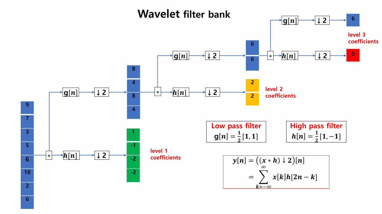
level 1 coefficients
level 2 coefficients
level 3 coefficients
High pass filter 𝒉𝒉 𝒏𝒏 = 𝟏𝟏
𝟑𝟑[𝟏𝟏,−𝟏𝟏]
Low pass filter g 𝒏𝒏 = 𝟏𝟏
𝟑𝟑[𝟏𝟏,𝟏𝟏]
∗
∗
∗
Wavelet filter bank
𝒚𝒚 𝒏𝒏 = 𝒙𝒙 ∗ 𝒉𝒉 ↓ 𝟑𝟑 𝒏𝒏
= � 𝒙𝒙 𝒌𝒌 𝒉𝒉[𝟑𝟑𝒏𝒏 − 𝒌𝒌]∞
𝒌𝒌=−∞

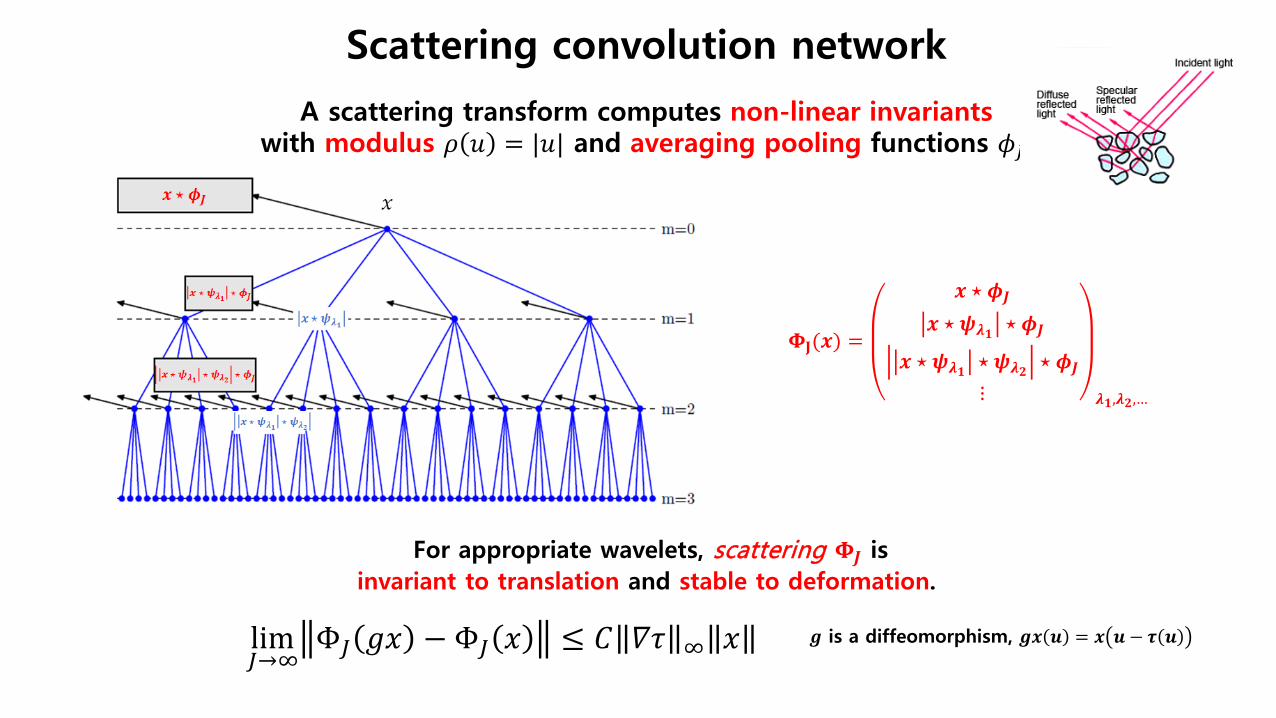
A scattering transform computes non-linear invariants with modulus 𝜌𝜌 𝑢𝑢 = |𝑢𝑢| and averaging pooling functions 𝜙𝜙𝐽𝐽.
Scattering convolution network
𝚽𝚽𝐉𝐉(𝒙𝒙) =
𝒙𝒙 ⋆ 𝝓𝝓𝑱𝑱
𝒙𝒙 ⋆ 𝝍𝝍𝝀𝝀𝟏𝟏 ⋆ 𝝓𝝓𝑱𝑱
𝒙𝒙 ⋆ 𝝍𝝍𝝀𝝀𝟏𝟏 ⋆ 𝝍𝝍𝝀𝝀𝟑𝟑 ⋆ 𝝓𝝓𝑱𝑱
⋮ 𝝀𝝀𝟏𝟏,𝝀𝝀𝟑𝟑,…
lim𝐽𝐽→∞
Φ𝐽𝐽 𝑔𝑔𝑥𝑥 − Φ𝐽𝐽 𝑥𝑥 ≤ 𝐶𝐶 𝛻𝛻𝜏𝜏 ∞ 𝑥𝑥
For appropriate wavelets, scattering 𝚽𝚽𝑱𝑱 is invariant to translation and stable to deformation.
𝒊𝒊 is a diffeomorphism, 𝒊𝒊𝒙𝒙 𝒖𝒖 = 𝒙𝒙 𝒖𝒖 − 𝝉𝝉 𝒖𝒖

: average
: detail(backward difference)
𝒙𝒙 ⋆ 𝝓𝝓𝟑𝟑 𝒙𝒙 ⋆ 𝝍𝝍𝟑𝟑
𝒙𝒙 ⋆ 𝝍𝝍𝟑𝟑
𝒙𝒙 ⋆ 𝝍𝝍𝟏𝟏
Wavelet coefficients: 𝒲𝒲𝑥𝑥 =𝑥𝑥 ⋆ 𝜙𝜙3𝑥𝑥 ⋆ 𝜓𝜓𝑗𝑗 𝑗𝑗≤3
Example of discrete Haar Wavelet Transform
for sound signal
Scattering convolution network
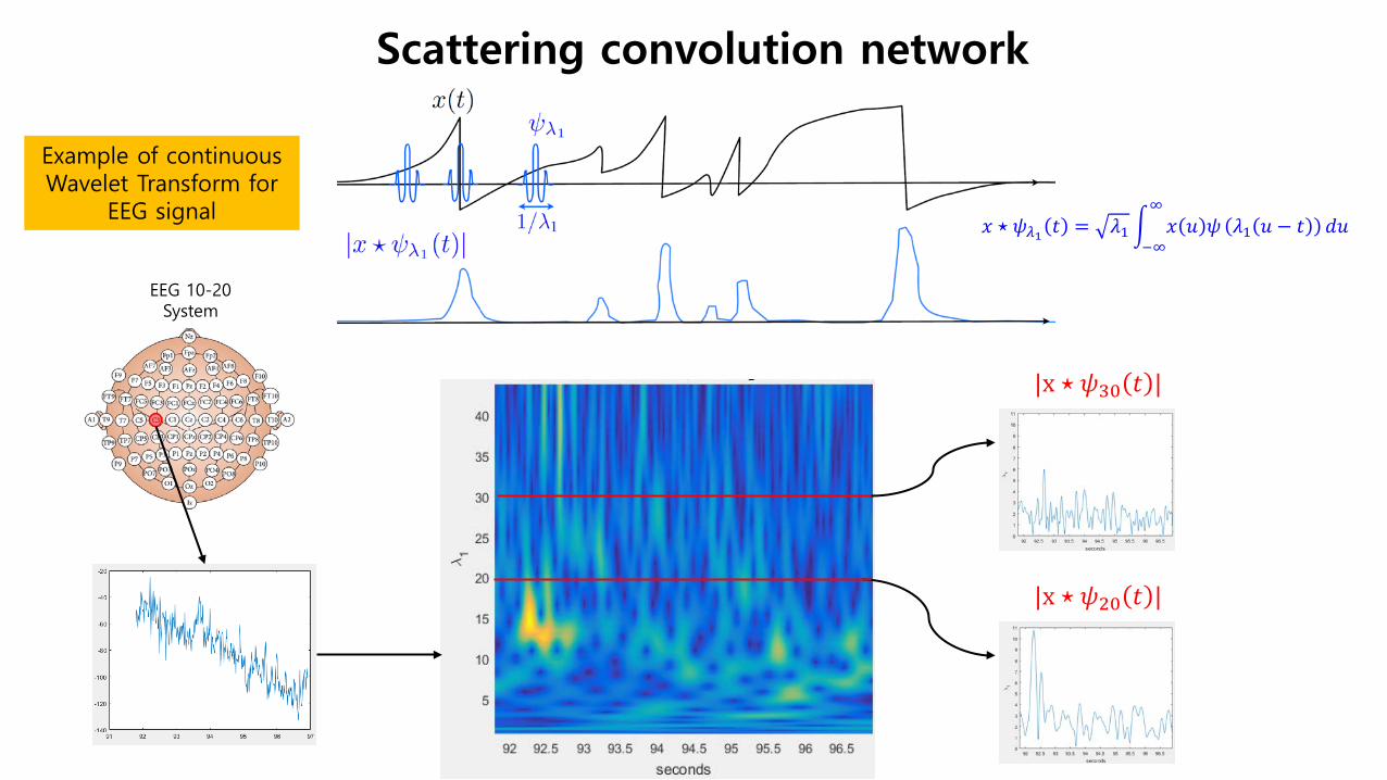
EEG 10-20 System
|x ⋆ 𝜓𝜓30 𝑡𝑡 |
|x ⋆ 𝜓𝜓20 𝑡𝑡 |
Example of continuous Wavelet Transform for
EEG signal
Scattering convolution network
𝑥𝑥 ⋆ 𝜓𝜓𝜆𝜆1 𝑡𝑡 = 𝜆𝜆1 � 𝑥𝑥 𝑢𝑢 𝜓𝜓 𝜆𝜆1 𝑢𝑢 − 𝑡𝑡∞
−∞𝑑𝑑𝑢𝑢
A scattering transform computes non-linear invariants with modulus 𝜌𝜌 𝑢𝑢 = |𝑢𝑢| and averaging pooling functions 𝜙𝜙𝐽𝐽.
Scattering convolution network
𝚽𝚽𝐉𝐉(𝒙𝒙) =
𝒙𝒙 ⋆ 𝝓𝝓𝑱𝑱
𝒙𝒙 ⋆ 𝝍𝝍𝝀𝝀𝟏𝟏 ⋆ 𝝓𝝓𝑱𝑱
𝒙𝒙 ⋆ 𝝍𝝍𝝀𝝀𝟏𝟏 ⋆ 𝝍𝝍𝝀𝝀𝟑𝟑 ⋆ 𝝓𝝓𝑱𝑱
⋮ 𝝀𝝀𝟏𝟏,𝝀𝝀𝟑𝟑,…
lim𝐽𝐽→∞
Φ𝐽𝐽 𝑔𝑔𝑥𝑥 − Φ𝐽𝐽 𝑥𝑥 ≤ 𝐶𝐶 𝛻𝛻𝜏𝜏 ∞ 𝑥𝑥
For appropriate wavelets, scattering 𝚽𝚽𝑱𝑱 is invariant to translation and stable to deformation.
𝒊𝒊 is a diffeomorphism, 𝒊𝒊𝒙𝒙 𝒖𝒖 = 𝒙𝒙 𝒖𝒖 − 𝝉𝝉 𝒖𝒖
𝒙𝒙 ⋆ 𝝍𝝍𝝀𝝀𝟏𝟏 ⋆ 𝝍𝝍𝝀𝝀𝟑𝟑 ⋆ 𝝓𝝓𝑱𝑱
𝜆𝜆2
𝜆𝜆1
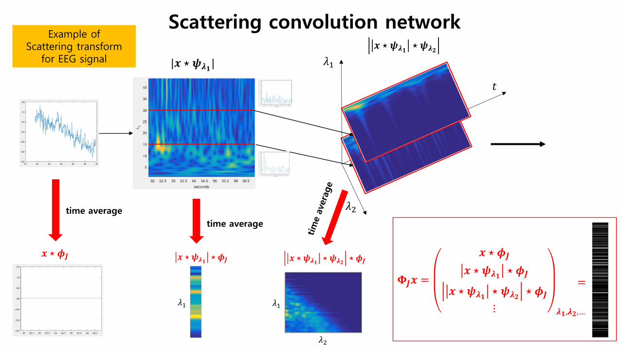
𝒙𝒙 ⋆ 𝝍𝝍𝝀𝝀𝟏𝟏 ⋆ 𝝓𝝓𝑱𝑱
𝜆𝜆1
𝒙𝒙 ⋆ 𝝓𝝓𝑱𝑱
Scattering convolution network Example of
Scattering transform for EEG signal
𝒙𝒙 ⋆ 𝝍𝝍𝝀𝝀𝟏𝟏 ⋆ 𝝍𝝍𝝀𝝀𝟑𝟑
𝜆𝜆1
𝑡𝑡
𝜆𝜆2
|𝒙𝒙 ⋆ 𝝍𝝍𝝀𝝀𝟏𝟏|
time average time average
𝚽𝚽𝑱𝑱𝒙𝒙 =
𝒙𝒙 ⋆ 𝝓𝝓𝑱𝑱
𝒙𝒙 ⋆ 𝝍𝝍𝝀𝝀𝟏𝟏 ⋆ 𝝓𝝓𝑱𝑱
𝒙𝒙 ⋆ 𝝍𝝍𝝀𝝀𝟏𝟏 ⋆ 𝝍𝝍𝝀𝝀𝟑𝟑 ⋆ 𝝓𝝓𝑱𝑱
⋮ 𝝀𝝀𝟏𝟏,𝝀𝝀𝟑𝟑,…
=

Deep learning: Convolution Neural Network
=
Handwritten digit recognition
=
0000010000
Φ = 𝑓𝑓0 𝒇𝒇 𝑓𝑓0 =
= 𝜎𝜎 𝜎𝜎 𝑠𝑠 =1
1 + 𝑒𝑒−𝑠𝑠
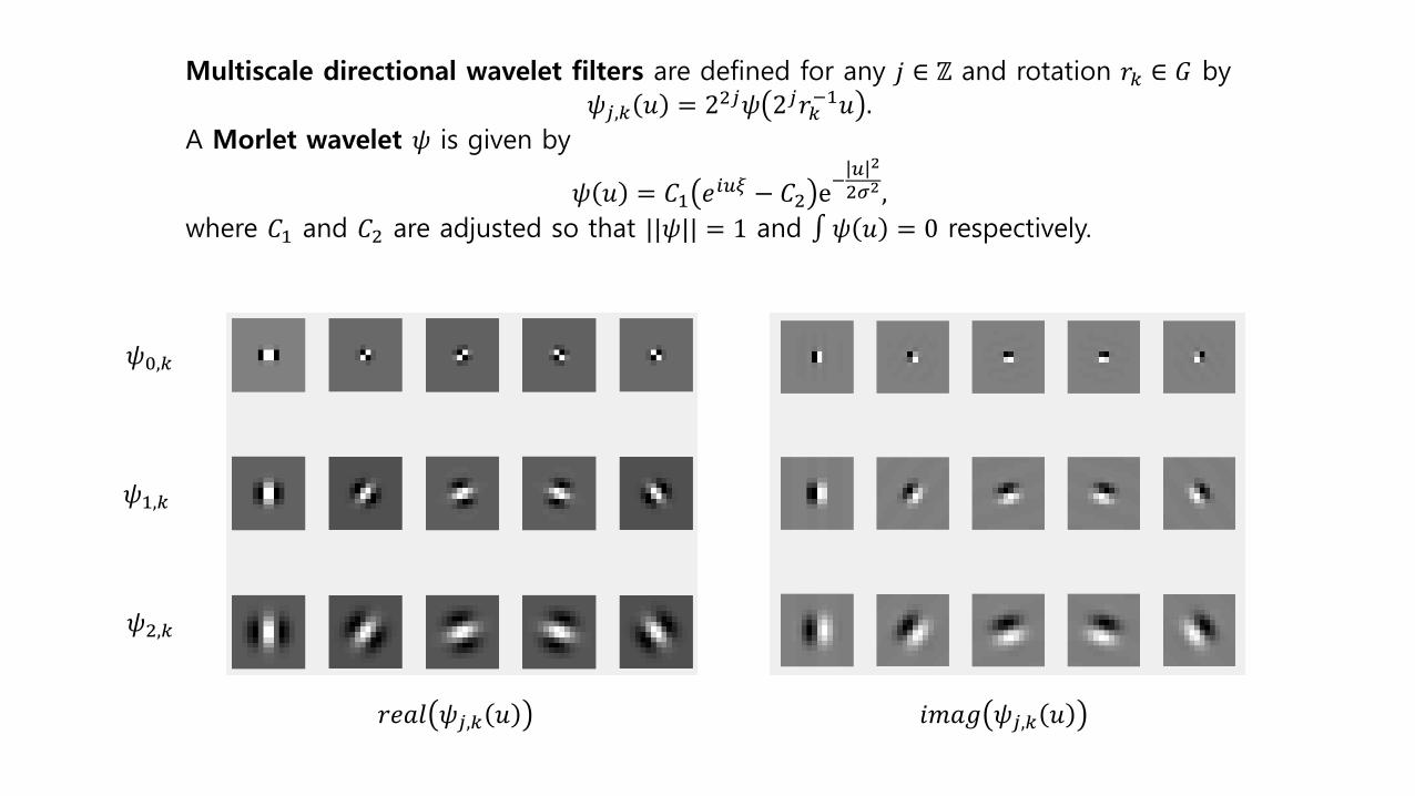
Multiscale directional wavelet filters are defined for any 𝑗𝑗 ∈ ℤ and rotation 𝑟𝑟𝑘𝑘 ∈ 𝐺𝐺 by 𝜓𝜓𝑗𝑗,𝑘𝑘 𝑢𝑢 = 22𝑗𝑗𝜓𝜓 2𝑗𝑗𝑟𝑟𝑘𝑘−1𝑢𝑢 .
A Morlet wavelet 𝜓𝜓 is given by
𝜓𝜓 𝑢𝑢 = 𝐶𝐶1 𝑒𝑒𝑖𝑖𝑖𝑖𝜋𝜋 − 𝐶𝐶2 e−𝑖𝑖 2
2𝜎𝜎2 , where 𝐶𝐶1 and 𝐶𝐶2 are adjusted so that ||𝜓𝜓|| = 1 and ∫ 𝜓𝜓 𝑢𝑢 = 0 respectively.
𝑟𝑟𝑒𝑒𝑟𝑟𝑟𝑟 𝜓𝜓𝑗𝑗,𝑘𝑘 𝑢𝑢 𝑖𝑖𝑚𝑚𝑟𝑟𝑔𝑔 𝜓𝜓𝑗𝑗,𝑘𝑘 𝑢𝑢
𝜓𝜓0,𝑘𝑘
𝜓𝜓1,𝑘𝑘
𝜓𝜓2,𝑘𝑘
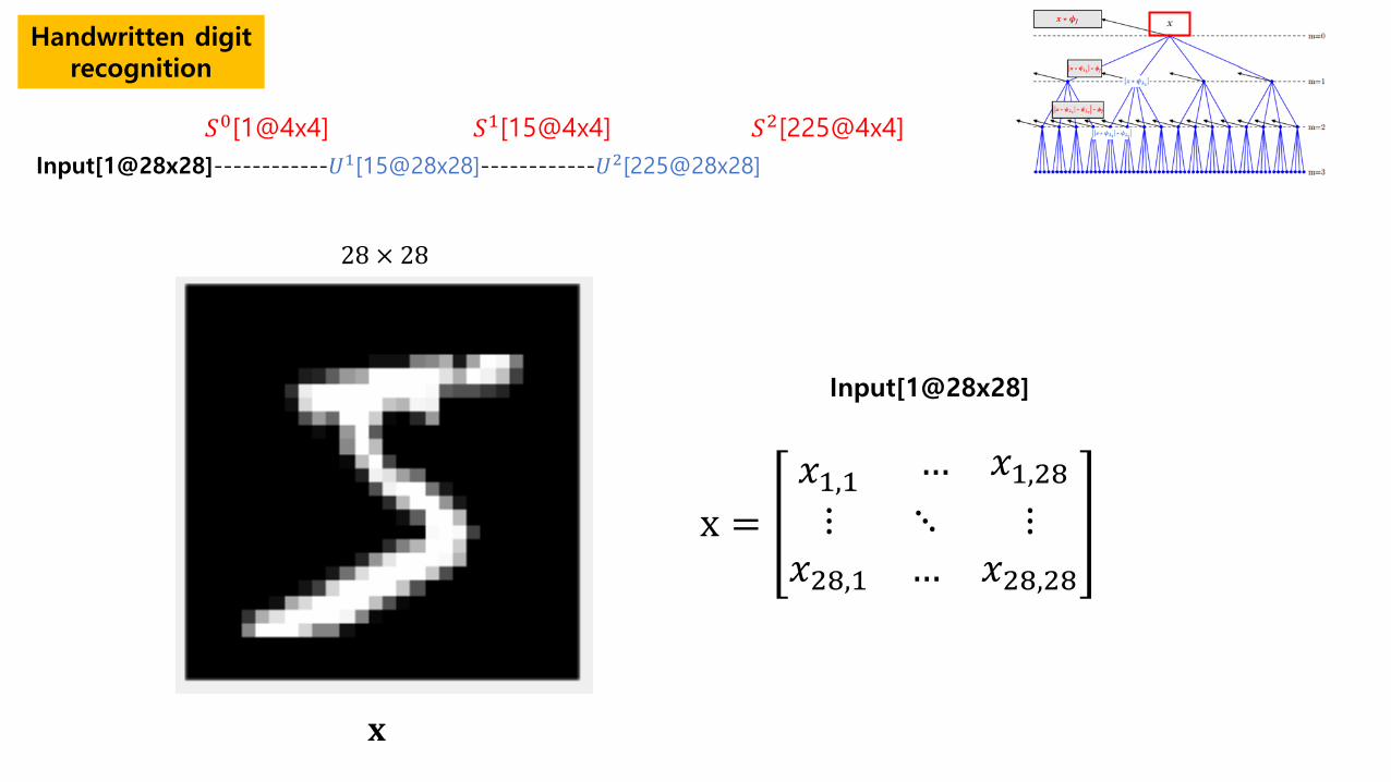
Handwritten digit recognition
Input[1@28x28]
x =𝑥𝑥1,1 … 𝑥𝑥1,28
⋮𝑥𝑥28,1
⋱ ⋮… 𝑥𝑥28,28
𝐱𝐱
Input[1@28x28]------------𝑈𝑈1[15@28x28]------------𝑈𝑈2[225@28x28]
𝑆𝑆0[1@4x4] 𝑆𝑆1[15@4x4] 𝑆𝑆2[225@4x4]
28 × 28
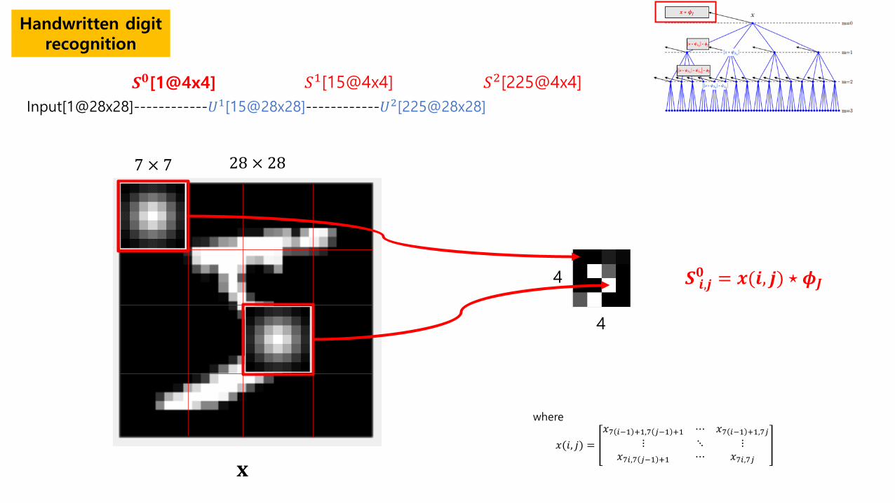
Handwritten digit recognition
4
4
𝐱𝐱
𝑺𝑺 𝒊𝒊,𝒋𝒋𝟎𝟎 = 𝒙𝒙(𝒊𝒊, 𝒋𝒋) ⋆ 𝝓𝝓𝑱𝑱
where
𝑥𝑥(𝑖𝑖, 𝑗𝑗) =𝑥𝑥7 𝑖𝑖−1 +1,7 𝑗𝑗−1 +1 ⋯ 𝑥𝑥7 𝑖𝑖−1 +1,7𝑗𝑗
⋮ ⋱ ⋮𝑥𝑥7𝑖𝑖,7 𝑗𝑗−1 +1 ⋯ 𝑥𝑥7𝑖𝑖,7𝑗𝑗
7 × 7
Input[1@28x28]------------𝑈𝑈1[15@28x28]------------𝑈𝑈2[225@28x28]
𝑺𝑺𝟎𝟎[1@4x4] 𝑆𝑆1[15@4x4] 𝑆𝑆2[225@4x4]
28 × 28

𝑼𝑼𝒊𝒊,𝒋𝒋𝟏𝟏 [𝝀𝝀𝟏𝟏] = 𝒙𝒙 𝒊𝒊, 𝒋𝒋 ⋆ 𝝍𝝍𝝀𝝀𝟏𝟏
Handwritten digit recognition
Input[1@28x28]------------𝑼𝑼𝟏𝟏[15@28x28]------------𝑈𝑈2[225@28x28]
𝑆𝑆0[1@4x4] 𝑆𝑆1[15@4x4] 𝑆𝑆2[225@4x4]
where 𝑥𝑥 𝑖𝑖, 𝑗𝑗 =𝑥𝑥�𝑖𝑖−6,𝑗𝑗−6 ⋯ 𝑥𝑥�𝑖𝑖−6,𝑗𝑗+7
⋮ ⋱ ⋮𝑥𝑥�𝑖𝑖+7,𝑗𝑗−6 ⋯ 𝑥𝑥�𝑖𝑖+7,𝑗𝑗+7
,
𝑥𝑥�𝛼𝛼,𝛽𝛽 = �𝑥𝑥𝛼𝛼,𝛽𝛽 𝑖𝑖𝑓𝑓 𝛼𝛼,𝛽𝛽 > 0,0 𝑜𝑜𝑡𝑡𝑜𝑒𝑒𝑟𝑟𝑤𝑤𝑖𝑖𝑠𝑠𝑒𝑒.
𝐱𝐱
= ⋆
14 × 14
𝜓𝜓0,𝑙𝑙1 𝜓𝜓1,𝑙𝑙1 𝜓𝜓2,𝑙𝑙1 (𝑟𝑟1 = 0,⋯ , 4) 𝑼𝑼𝟏𝟏
𝜆𝜆1 = 𝑘𝑘1, 𝑟𝑟1
28 × 28

Handwritten digit recognition
Input[1@28x28]------------U1[15@28x28]------------U2[225@28x28]
S0[1@4x4] S1[15@4x4] S2[225@4x4]
𝑺𝑺𝒊𝒊,𝒋𝒋𝟏𝟏 [𝝀𝝀𝟏𝟏] = 𝑼𝑼𝟏𝟏[𝝀𝝀𝟏𝟏](𝒊𝒊, 𝒋𝒋) ⋆ 𝝓𝝓𝑱𝑱
where
𝑈𝑈1[𝜆𝜆1](𝑖𝑖, 𝑗𝑗) =𝑈𝑈7 𝑖𝑖−1 +1,7 𝑗𝑗−1 +11 [𝜆𝜆1] ⋯ 𝑈𝑈7 𝑖𝑖−1 +1,7𝑗𝑗
1 [𝜆𝜆1] ⋮ ⋱ ⋮
𝑈𝑈7𝑖𝑖,7 𝑗𝑗−1 +11 [𝜆𝜆1] ⋯ 𝑈𝑈7𝑖𝑖,7𝑗𝑗1 [𝜆𝜆1]
𝜙𝜙𝐽𝐽 𝑈𝑈1
28 × 28
7 × 7
4 × 4
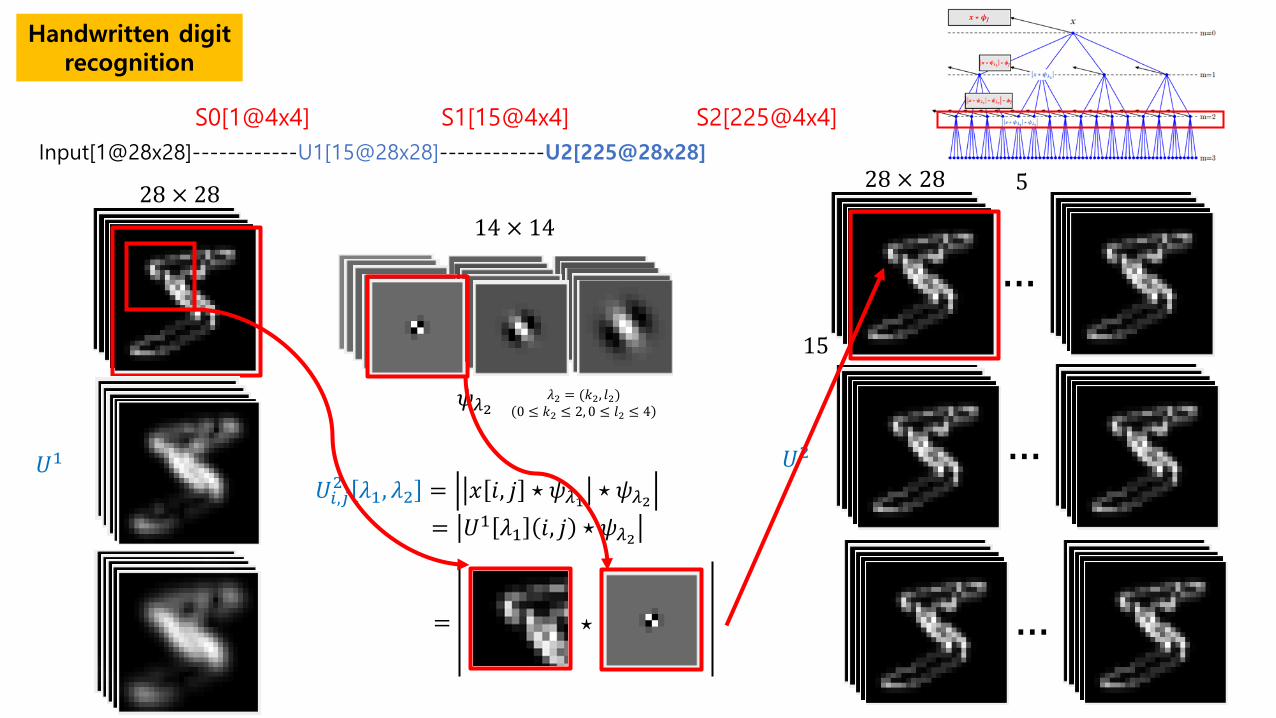
Handwritten digit recognition
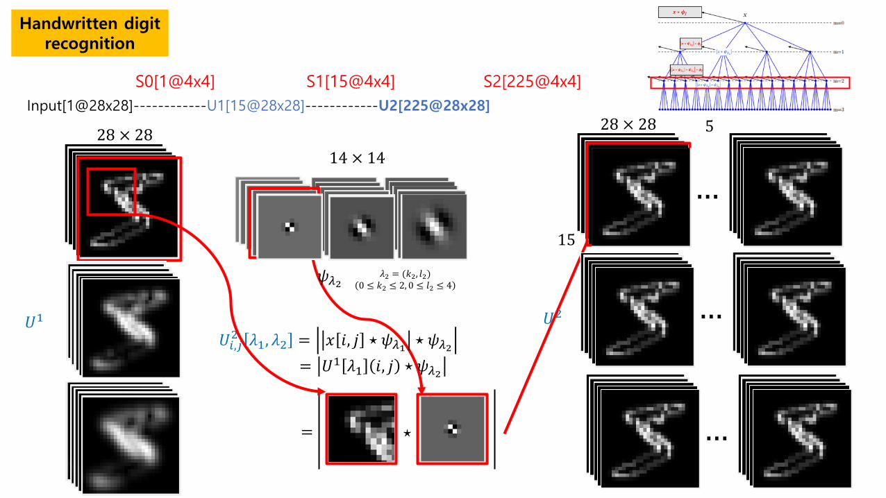
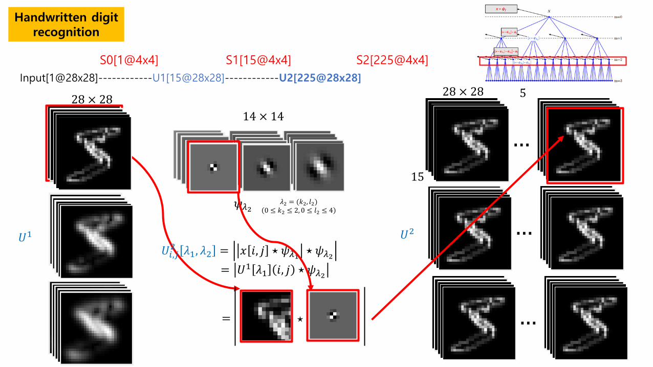
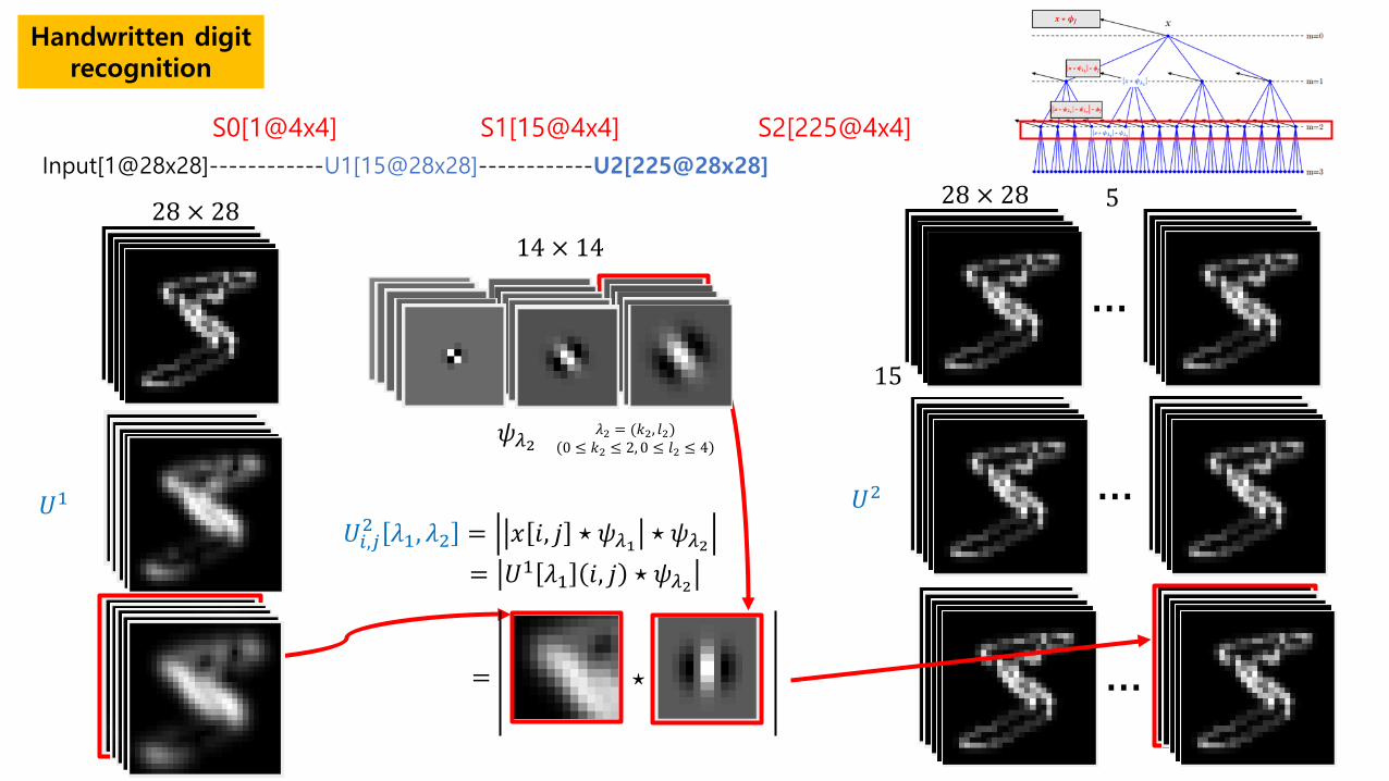
Input[1@28x28]------------U1[15@28x28]------------U2[225@28x28]
S0[1@4x4] S1[15@4x4] S2[225@4x4]
𝑈𝑈1
14 × 14
𝜓𝜓𝜆𝜆2 𝜆𝜆2 = (𝑘𝑘2, 𝑟𝑟2) 0 ≤ 𝑘𝑘2 ≤ 2, 0 ≤ 𝑟𝑟2 ≤ 4
…
…
… = ⋆
15
5
𝑈𝑈𝑖𝑖,𝑗𝑗2 𝜆𝜆1, 𝜆𝜆2 = 𝑥𝑥 𝑖𝑖, 𝑗𝑗 ⋆ 𝜓𝜓𝜆𝜆1 ⋆ 𝜓𝜓𝜆𝜆2 = 𝑈𝑈1 𝜆𝜆1 𝑖𝑖, 𝑗𝑗 ⋆ 𝜓𝜓𝜆𝜆2
𝑈𝑈2
28 × 28 28 × 28
Handwritten digit recognition
Input[1@28x28]------------U1[15@28x28]------------U2[225@28x28]
S0[1@4x4] S1[15@4x4] S2[225@4x4]
𝑈𝑈1
14 × 14
𝜓𝜓𝜆𝜆2 𝜆𝜆2 = (𝑘𝑘2, 𝑟𝑟2) 0 ≤ 𝑘𝑘2 ≤ 2, 0 ≤ 𝑟𝑟2 ≤ 4
…
…
… = ⋆
15
5
𝑈𝑈𝑖𝑖,𝑗𝑗2 𝜆𝜆1, 𝜆𝜆2 = 𝑥𝑥 𝑖𝑖, 𝑗𝑗 ⋆ 𝜓𝜓𝜆𝜆1 ⋆ 𝜓𝜓𝜆𝜆2 = 𝑈𝑈1 𝜆𝜆1 𝑖𝑖, 𝑗𝑗 ⋆ 𝜓𝜓𝜆𝜆2
𝑈𝑈2
28 × 28 28 × 28

Handwritten digit recognition
Input[1@28x28]------------U1[15@28x28]------------U2[225@28x28]
S0[1@4x4] S1[15@4x4] S2[225@4x4]
𝑈𝑈1
14 × 14
𝜓𝜓𝜆𝜆2 𝜆𝜆2 = (𝑘𝑘2, 𝑟𝑟2) 0 ≤ 𝑘𝑘2 ≤ 2, 0 ≤ 𝑟𝑟2 ≤ 4
…
…
… = ⋆
15
5
𝑈𝑈𝑖𝑖,𝑗𝑗2 𝜆𝜆1, 𝜆𝜆2 = 𝑥𝑥 𝑖𝑖, 𝑗𝑗 ⋆ 𝜓𝜓𝜆𝜆1 ⋆ 𝜓𝜓𝜆𝜆2 = 𝑈𝑈1 𝜆𝜆1 𝑖𝑖, 𝑗𝑗 ⋆ 𝜓𝜓𝜆𝜆2
𝑈𝑈2
28 × 28 28 × 28
Handwritten digit recognition
Input[1@28x28]------------U1[15@28x28]------------U2[225@28x28]
S0[1@4x4] S1[15@4x4] S2[225@4x4]
𝑈𝑈1
14 × 14
𝜓𝜓𝜆𝜆2 𝜆𝜆2 = (𝑘𝑘2, 𝑟𝑟2) 0 ≤ 𝑘𝑘2 ≤ 2, 0 ≤ 𝑟𝑟2 ≤ 4
…
…
… = ⋆
15
5
𝑈𝑈𝑖𝑖,𝑗𝑗2 𝜆𝜆1, 𝜆𝜆2 = 𝑥𝑥 𝑖𝑖, 𝑗𝑗 ⋆ 𝜓𝜓𝜆𝜆1 ⋆ 𝜓𝜓𝜆𝜆2 = 𝑈𝑈1 𝜆𝜆1 𝑖𝑖, 𝑗𝑗 ⋆ 𝜓𝜓𝜆𝜆2
𝑈𝑈2
28 × 28 28 × 28
Handwritten digit recognition
Input[1@28x28]------------U1[15@28x28]------------U2[225@28x28]
S0[1@4x4] S1[15@4x4] S2[225@4x4]
𝑈𝑈1 𝑈𝑈𝑖𝑖,𝑗𝑗2 𝜆𝜆1, 𝜆𝜆2 = 𝑥𝑥 𝑖𝑖, 𝑗𝑗 ⋆ 𝜓𝜓𝜆𝜆1 ⋆ 𝜓𝜓𝜆𝜆2
= 𝑈𝑈1 𝜆𝜆1 𝑖𝑖, 𝑗𝑗 ⋆ 𝜓𝜓𝜆𝜆2
28 × 28 14 × 14
𝜓𝜓𝜆𝜆2 𝜆𝜆2 = (𝑘𝑘2, 𝑟𝑟2) 0 ≤ 𝑘𝑘2 ≤ 2, 0 ≤ 𝑟𝑟2 ≤ 4
…
…
… = ⋆
15
5
𝑈𝑈2
28 × 28
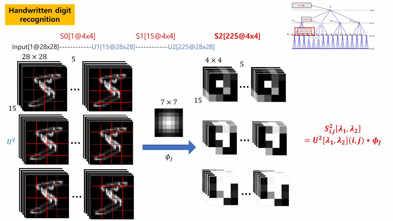
Handwritten digit recognition
Input[1@28x28]------------U1[15@28x28]------------U2[225@28x28]
S0[1@4x4] S1[15@4x4] S2[225@4x4]
…
…
…
𝜙𝜙𝐽𝐽
𝑈𝑈2
28 × 28
15
5
7 × 7
…
…
…
𝑺𝑺𝒊𝒊,𝒋𝒋𝟑𝟑 𝝀𝝀𝟏𝟏,𝝀𝝀𝟑𝟑 = 𝑼𝑼𝟑𝟑[𝝀𝝀𝟏𝟏,𝝀𝝀𝟑𝟑](𝒊𝒊, 𝒋𝒋) ⋆ 𝝓𝝓𝑱𝑱
4 × 4
15
5
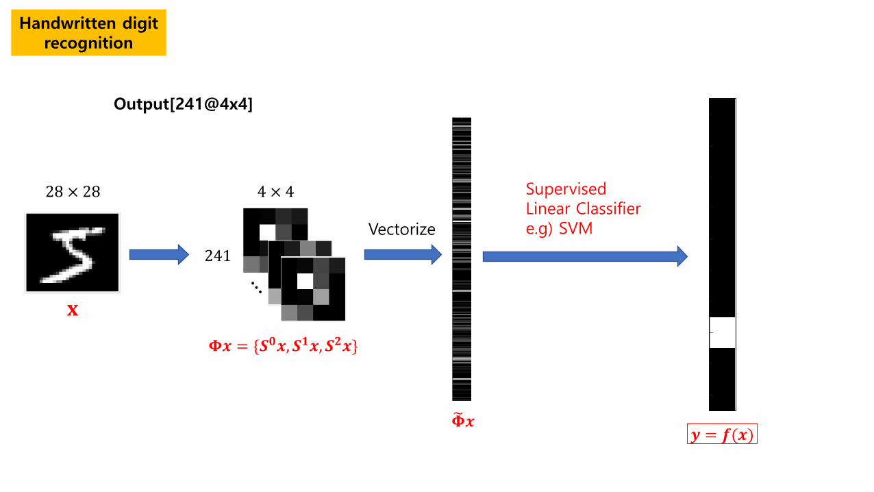
Handwritten digit recognition
Output[241@4x4]
𝚽𝚽𝒙𝒙 = {𝑺𝑺𝟎𝟎𝒙𝒙,𝑺𝑺𝟏𝟏𝒙𝒙,𝑺𝑺𝟑𝟑𝒙𝒙}
⋱
4 × 4
241
𝚽𝚽�𝒙𝒙
Vectorize
𝐱𝐱
28 × 28 Supervised Linear Classifier e.g) SVM
𝒚𝒚 = 𝒇𝒇(𝒙𝒙)
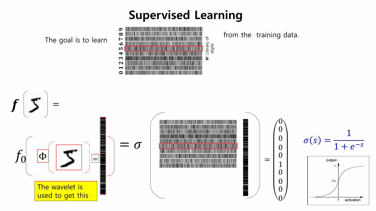
Supervised Learning
The goal is to learn
Φ =
𝟎𝟎 𝟏𝟏 𝟑𝟑 𝟑𝟑 𝟒𝟒 𝟓𝟓 𝟐𝟐 𝟕𝟕 𝟖𝟖 𝟗𝟗
𝑾𝑾: L
ibra
ry o
f dig
its
= 𝒇𝒇
=
0000010000
= 𝜎𝜎 𝜎𝜎 𝑠𝑠 =1
1 + 𝑒𝑒−𝑠𝑠
𝑓𝑓0
from the training data.
The wavelet is used to get this
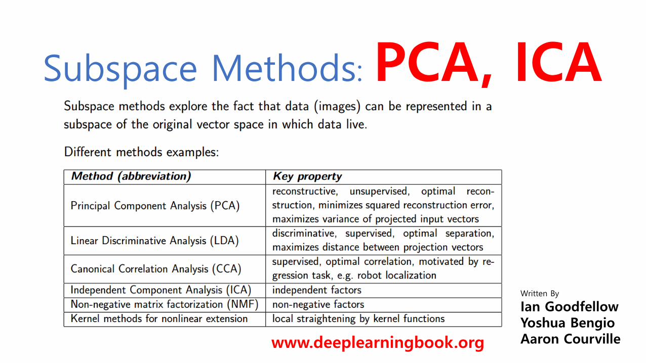
Written By
Ian Goodfellow Yoshua Bengio Aaron Courville
Subspace Methods: PCA, ICA
www.deeplearningbook.org

Basics in Principal Component Analysis
Suppose we would like to apply lossy compression to a collection of m points 𝒙𝒙 𝟏𝟏 ,⋯ ,𝒙𝒙 𝒎𝒎 ⊂ 𝑹𝑹𝒏𝒏. Lossy compression means storing the points in a way that requires less memory but may lose some precision.
𝒙𝒙 𝟏𝟏 ,⋯ ,𝒙𝒙 𝟑𝟑𝟑𝟑 ⊂ 𝑹𝑹𝒏𝒏
𝐧𝐧 = 𝟑𝟑𝟑𝟑𝟏𝟏 × 𝟑𝟑𝟐𝟐𝟏𝟏
𝒙𝒙 𝟏𝟏
𝒙𝒙 𝟑𝟑𝟑𝟑 Slide Credit: Vaclav
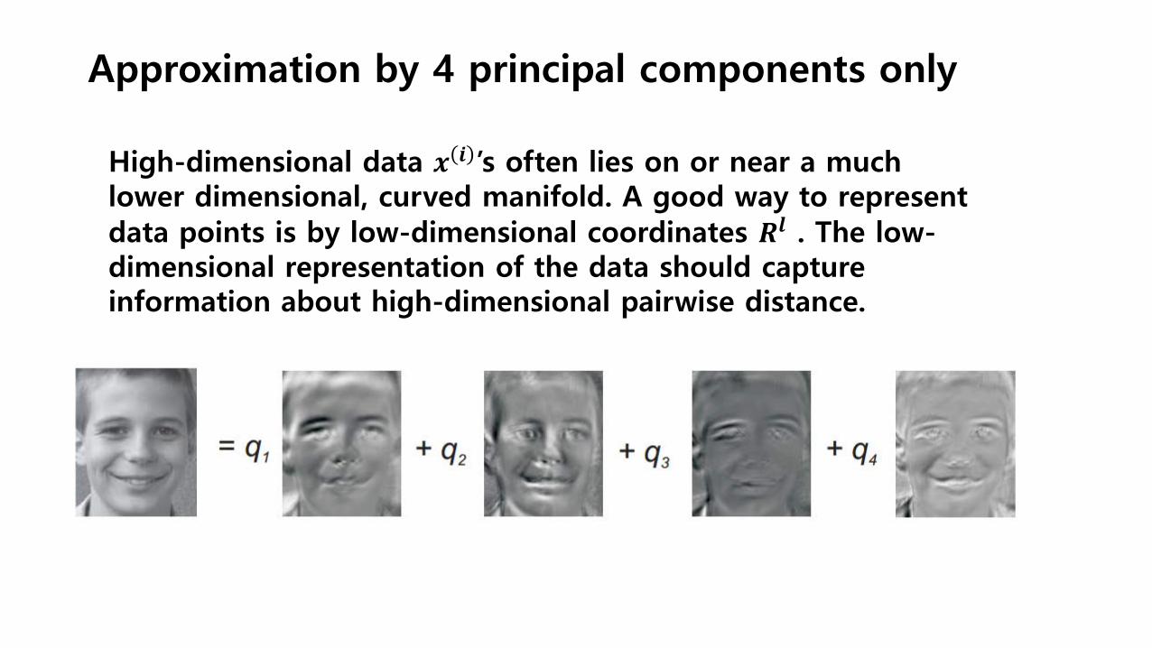
Approximation by 4 principal components only
High-dimensional data 𝒙𝒙 𝒊𝒊 ’s often lies on or near a much lower dimensional, curved manifold. A good way to represent data points is by low-dimensional coordinates 𝑹𝑹𝒅𝒅 . The low-dimensional representation of the data should capture information about high-dimensional pairwise distance.
Approximation by 4 principal components only
𝒙𝒙 𝟏𝟏 ,⋯ ,𝒙𝒙 𝟑𝟑𝟑𝟑 ⊂ 𝑹𝑹𝒏𝒏 𝐧𝐧 = 𝟑𝟑𝟑𝟑𝟏𝟏 × 𝟑𝟑𝟐𝟐𝟏𝟏 𝒅𝒅𝒊𝒊𝒎𝒎𝒅𝒅𝒏𝒏𝒅𝒅𝒊𝒊𝒅𝒅𝒏𝒏𝒅𝒅𝒅𝒅 𝒊𝒊𝒎𝒎𝒅𝒅𝒊𝒊𝒅𝒅𝒅𝒅 𝟒𝟒 𝒅𝒅𝒊𝒊𝒎𝒎𝒅𝒅𝒏𝒏𝒅𝒅𝒊𝒊𝒅𝒅𝒏𝒏𝒅𝒅𝒅𝒅 𝒊𝒊𝒎𝒎𝒅𝒅𝒊𝒊𝒅𝒅𝒅𝒅
Slide Credit: Vaclav
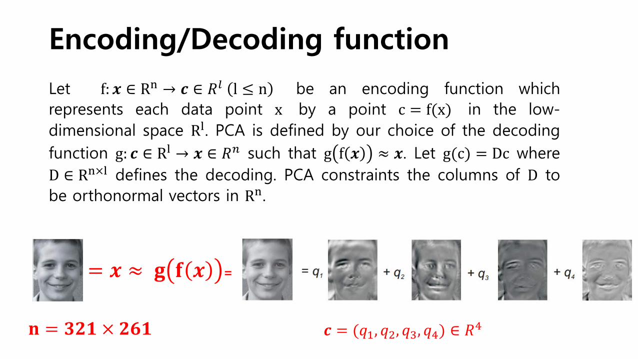
Encoding/Decoding function
Let f:𝒙𝒙 ∈ Rn → 𝒄𝒄 ∈ 𝑅𝑅𝑙𝑙 l ≤ n be an encoding function which represents each data point x by a point c = f(x) in the low-dimensional space Rl. PCA is defined by our choice of the decoding function g: 𝒄𝒄 ∈ Rl → 𝒙𝒙 ∈ 𝑅𝑅𝑛𝑛 such that g f 𝒙𝒙 ≈ 𝒙𝒙. Let g(c) = Dc where D ∈ Rn×l defines the decoding. PCA constraints the columns of D to be orthonormal vectors in Rn.
= 𝒙𝒙 ≈ 𝐠𝐠 𝐟𝐟 𝒙𝒙 =
𝒄𝒄 = (𝑞𝑞1, 𝑞𝑞2, 𝑞𝑞3, 𝑞𝑞4) ∈ 𝑅𝑅4 𝐧𝐧 = 𝟑𝟑𝟑𝟑𝟏𝟏 × 𝟑𝟑𝟐𝟐𝟏𝟏

Let 𝐠𝐠(𝐜𝐜) = 𝐃𝐃𝐜𝐜 where 𝐃𝐃 ∈ 𝑹𝑹𝐧𝐧×𝒅𝒅 defines the decoding.
𝐠𝐠 𝐜𝐜 𝐃𝐃
= [ ] 𝟎𝟎.𝟎𝟎𝟕𝟕𝟖𝟖𝟎𝟎.𝟎𝟎𝟐𝟐𝟑𝟑−𝟎𝟎.𝟏𝟏𝟖𝟖𝟑𝟑𝟎𝟎.𝟏𝟏𝟕𝟕𝟗𝟗
1ST column 2nd column 3rd column 4th column
𝐜𝐜
Slide Credit: Vaclav
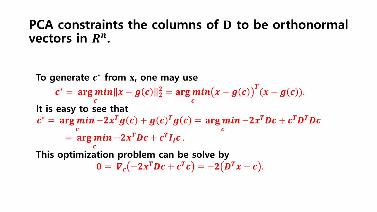
PCA constraints the columns of 𝐃𝐃 to be orthonormal vectors in 𝑹𝑹𝒏𝒏.
To generate 𝒄𝒄∗ from 𝐱𝐱, one may use
𝒄𝒄∗ = 𝐚𝐚𝐚𝐚𝐠𝐠 𝒎𝒎𝒊𝒊𝒏𝒏𝒄𝒄
𝒙𝒙 − 𝒊𝒊 𝒄𝒄 𝟑𝟑𝟑𝟑 = 𝐚𝐚𝐚𝐚𝐠𝐠 𝒎𝒎𝒊𝒊𝒏𝒏
𝒄𝒄𝒙𝒙 − 𝒊𝒊 𝒄𝒄 𝑻𝑻(𝒙𝒙 − 𝒊𝒊 𝒄𝒄 ).
It is easy to see that 𝒄𝒄∗ = 𝐚𝐚𝐚𝐚𝐠𝐠 𝒎𝒎𝒊𝒊𝒏𝒏
𝒄𝒄−𝟑𝟑𝒙𝒙𝑻𝑻𝒊𝒊 𝒄𝒄 + 𝒊𝒊 𝒄𝒄 𝑻𝑻𝒊𝒊 𝒄𝒄 = 𝐚𝐚𝐚𝐚𝐠𝐠 𝒎𝒎𝒊𝒊𝒏𝒏
𝒄𝒄−𝟑𝟑𝒙𝒙𝑻𝑻𝑫𝑫𝒄𝒄 + 𝒄𝒄𝑻𝑻𝑫𝑫𝑻𝑻𝑫𝑫𝒄𝒄
= 𝐚𝐚𝐚𝐚𝐠𝐠 𝒎𝒎𝒊𝒊𝒏𝒏𝒄𝒄
−𝟑𝟑𝒙𝒙𝑻𝑻𝑫𝑫𝒄𝒄 + 𝒄𝒄𝑻𝑻𝑰𝑰𝒅𝒅𝒄𝒄 .
This optimization problem can be solve by 𝟎𝟎 = 𝜵𝜵𝒄𝒄 −𝟑𝟑𝒙𝒙𝑻𝑻𝑫𝑫𝒄𝒄 + 𝒄𝒄𝑻𝑻𝒄𝒄 = −𝟑𝟑 𝑫𝑫𝑻𝑻𝒙𝒙 − 𝒄𝒄 .

How to choose encoding matrix 𝑫𝑫∗
By defining the encoding function 𝐟𝐟 𝒙𝒙 = 𝑫𝑫𝑻𝑻𝒙𝒙, we can define the PCA reconstruction operation
𝐚𝐚 𝒙𝒙 = 𝒊𝒊 𝒇𝒇 𝒙𝒙 = 𝑫𝑫𝑫𝑫𝑻𝑻𝒙𝒙. An encoding matrix 𝑫𝑫∗ can be chosen by
𝑫𝑫∗ = 𝐚𝐚𝐚𝐚𝐠𝐠 𝒎𝒎𝒊𝒊𝒏𝒏𝑫𝑫
∑ 𝒙𝒙 𝒊𝒊 − 𝒓𝒓 𝒙𝒙 𝒊𝒊𝟑𝟑𝟑𝟑
𝒊𝒊 subject to 𝑫𝑫𝑻𝑻𝑫𝑫 = 𝑰𝑰𝒅𝒅.
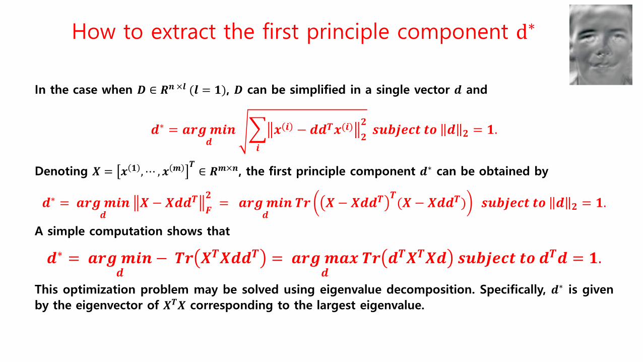
How to extract the first principle component d∗
In the case when 𝑫𝑫 ∈ 𝑹𝑹𝒏𝒏 ×𝒅𝒅 (𝒅𝒅 = 𝟏𝟏), 𝑫𝑫 can be simplified in a single vector 𝒅𝒅 and
𝒅𝒅∗ = 𝒅𝒅𝒓𝒓𝒊𝒊 𝒎𝒎𝒊𝒊𝒏𝒏𝒅𝒅
� 𝒙𝒙 𝒊𝒊 − 𝒅𝒅𝒅𝒅𝑻𝑻𝒙𝒙(𝒊𝒊)𝟑𝟑𝟑𝟑
𝒊𝒊
𝒅𝒅𝒖𝒖𝒔𝒔𝒋𝒋𝒅𝒅𝒄𝒄𝒔𝒔 𝒔𝒔𝒅𝒅 𝒅𝒅 𝟑𝟑 = 𝟏𝟏.
Denoting 𝑿𝑿 = 𝒙𝒙 𝟏𝟏 ,⋯ ,𝒙𝒙 𝒎𝒎 𝑻𝑻∈ 𝑹𝑹𝒎𝒎×𝒏𝒏, the first principle component 𝒅𝒅∗ can be obtained by
𝒅𝒅∗ = 𝒅𝒅𝒓𝒓𝒊𝒊 𝒎𝒎𝒊𝒊𝒏𝒏𝒅𝒅
𝑿𝑿 − 𝑿𝑿𝒅𝒅𝒅𝒅𝑻𝑻 𝑭𝑭𝟑𝟑 = 𝒅𝒅𝒓𝒓𝒊𝒊 𝒎𝒎𝒊𝒊𝒏𝒏
𝒅𝒅 𝑻𝑻𝒓𝒓 𝑿𝑿 − 𝑿𝑿𝒅𝒅𝒅𝒅𝑻𝑻 𝑻𝑻(𝑿𝑿 − 𝑿𝑿𝒅𝒅𝒅𝒅𝑻𝑻) 𝒅𝒅𝒖𝒖𝒔𝒔𝒋𝒋𝒅𝒅𝒄𝒄𝒔𝒔 𝒔𝒔𝒅𝒅 𝒅𝒅 𝟑𝟑 = 𝟏𝟏.
A simple computation shows that
𝒅𝒅∗ = 𝒅𝒅𝒓𝒓𝒊𝒊 𝒎𝒎𝒊𝒊𝒏𝒏𝒅𝒅
− 𝑻𝑻𝒓𝒓 𝑿𝑿𝑻𝑻𝑿𝑿𝒅𝒅𝒅𝒅𝑻𝑻 = 𝒅𝒅𝒓𝒓𝒊𝒊 𝒎𝒎𝒅𝒅𝒙𝒙𝒅𝒅
𝑻𝑻𝒓𝒓 𝒅𝒅𝑻𝑻𝑿𝑿𝑻𝑻𝑿𝑿𝒅𝒅 𝒅𝒅𝒖𝒖𝒔𝒔𝒋𝒋𝒅𝒅𝒄𝒄𝒔𝒔 𝒔𝒔𝒅𝒅 𝒅𝒅𝑻𝑻𝒅𝒅 = 𝟏𝟏.
This optimization problem may be solved using eigenvalue decomposition. Specifically, 𝒅𝒅∗ is given by the eigenvector of 𝑿𝑿𝑻𝑻𝑿𝑿 corresponding to the largest eigenvalue.

32nd row
1st row
= 𝒅𝒅∗= 𝒅𝒅𝒓𝒓𝒊𝒊 𝒎𝒎𝒊𝒊𝒏𝒏𝒅𝒅
𝑿𝑿 − 𝑿𝑿𝒅𝒅𝒅𝒅𝑻𝑻 𝑭𝑭𝟑𝟑
The first principle component
Slide Credit: Vaclav
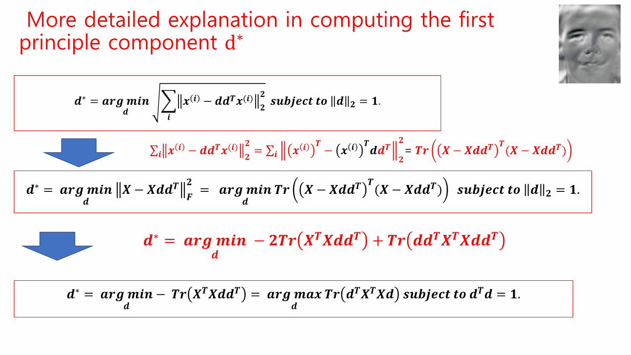
More detailed explanation in computing the first principle component d∗
𝒅𝒅∗ = 𝒅𝒅𝒓𝒓𝒊𝒊 𝒎𝒎𝒊𝒊𝒏𝒏𝒅𝒅
𝑿𝑿 − 𝑿𝑿𝒅𝒅𝒅𝒅𝑻𝑻 𝑭𝑭𝟑𝟑 = 𝒅𝒅𝒓𝒓𝒊𝒊 𝒎𝒎𝒊𝒊𝒏𝒏
𝒅𝒅 𝑻𝑻𝒓𝒓 𝑿𝑿 − 𝑿𝑿𝒅𝒅𝒅𝒅𝑻𝑻 𝑻𝑻(𝑿𝑿 − 𝑿𝑿𝒅𝒅𝒅𝒅𝑻𝑻) 𝒅𝒅𝒖𝒖𝒔𝒔𝒋𝒋𝒅𝒅𝒄𝒄𝒔𝒔 𝒔𝒔𝒅𝒅 𝒅𝒅 𝟑𝟑 = 𝟏𝟏.
𝒅𝒅∗ = 𝒅𝒅𝒓𝒓𝒊𝒊 𝒎𝒎𝒊𝒊𝒏𝒏𝒅𝒅
− 𝑻𝑻𝒓𝒓 𝑿𝑿𝑻𝑻𝑿𝑿𝒅𝒅𝒅𝒅𝑻𝑻 = 𝒅𝒅𝒓𝒓𝒊𝒊 𝒎𝒎𝒅𝒅𝒙𝒙𝒅𝒅
𝑻𝑻𝒓𝒓 𝒅𝒅𝑻𝑻𝑿𝑿𝑻𝑻𝑿𝑿𝒅𝒅 𝒅𝒅𝒖𝒖𝒔𝒔𝒋𝒋𝒅𝒅𝒄𝒄𝒔𝒔 𝒔𝒔𝒅𝒅 𝒅𝒅𝑻𝑻𝒅𝒅 = 𝟏𝟏.
∑ 𝒙𝒙 𝒊𝒊 − 𝒅𝒅𝒅𝒅𝑻𝑻𝒙𝒙(𝒊𝒊)𝟑𝟑𝟑𝟑
= ∑ 𝒙𝒙 𝒊𝒊 𝑻𝑻− 𝒙𝒙 𝒊𝒊 𝑻𝑻
𝒅𝒅𝒅𝒅𝑻𝑻𝟑𝟑
𝟑𝟑𝒊𝒊𝒊𝒊 = 𝑻𝑻𝒓𝒓 𝑿𝑿 − 𝑿𝑿𝒅𝒅𝒅𝒅𝑻𝑻 𝑻𝑻(𝑿𝑿 − 𝑿𝑿𝒅𝒅𝒅𝒅𝑻𝑻)
𝒅𝒅∗ = 𝒅𝒅𝒓𝒓𝒊𝒊 𝒎𝒎𝒊𝒊𝒏𝒏𝒅𝒅
� 𝒙𝒙 𝒊𝒊 − 𝒅𝒅𝒅𝒅𝑻𝑻𝒙𝒙(𝒊𝒊)𝟑𝟑𝟑𝟑
𝒊𝒊
𝒅𝒅𝒖𝒖𝒔𝒔𝒋𝒋𝒅𝒅𝒄𝒄𝒔𝒔 𝒔𝒔𝒅𝒅 𝒅𝒅 𝟑𝟑 = 𝟏𝟏.
𝒅𝒅∗ = 𝒅𝒅𝒓𝒓𝒊𝒊 𝒎𝒎𝒊𝒊𝒏𝒏𝒅𝒅
− 𝟑𝟑𝑻𝑻𝒓𝒓 𝑿𝑿𝑻𝑻𝑿𝑿𝒅𝒅𝒅𝒅𝑻𝑻 + 𝑻𝑻𝒓𝒓 𝒅𝒅𝒅𝒅𝑻𝑻𝑿𝑿𝑻𝑻𝑿𝑿𝒅𝒅𝒅𝒅𝑻𝑻
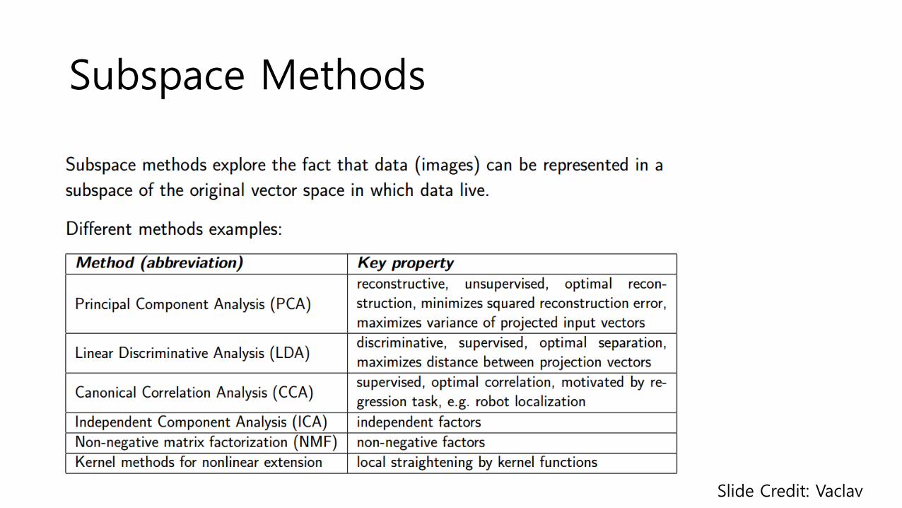
Subspace Methods
Slide Credit: Vaclav
Related Documents


![ME 697: INTELLIGENT SYSTEMS presentation/2016... · “Eggholder Function”[1] Constraints: 𝑔𝑔1= 𝑥𝑥+ 512 𝑔𝑔2= 512 −𝑥𝑥 𝑔𝑔3= 𝑦𝑦+ 512 𝑔𝑔4=](https://static.cupdf.com/doc/110x72/60569cd2f81b08010f55d532/me-697-intelligent-systems-presentation2016-aoeeggholder-functiona1-constraints.jpg)

