MA123, Chapter 3: The idea of limits (pp. 47-67, Gootman)

1/10 Chapter3.pdfUniversity Of Kentucky > Elementary Calculus and its Applications

MA123, Chapter 3: The idea of limits (pp. 47-67, Gootman)

Chapter Goals: • Evaluate limits.

• Evaluate one-sided limits.

• Understand the concepts of continuity and differentiability and their relationship.

Assignments: Assignment 04 Assignment 05

Earlier, the idea of limits came up naturally in the course of defining the derivative of a function at a point.

We now study limits more systematically. Computing a limit means computing what happens to the value of a

function as the variable in the expression gets closer and closer to (but does not equal) a particular value.

! The basic definition of limit: Let f be a function of x. The expression

limx→c

f(x) = L

means that as x gets closer and closer to c, through values both smaller and larger than c, but not equal to c,

then the values of f(x) get closer and closer to the value L.

Note: It may sometimes happen that the limit does not exist.

Example 1 (a): Use the tables to help evaluate limx→2

x2 + 8

x+ 2.

x gets close to 2 from the left

x 1.8 1.9 1.99 1.999

x2 + 8

x+ 2

x gets close to 2 from the right

2.001 2.01 2.1 2.2 x

x2 + 8

x+ 2

Example 1 (b): Suppose that, instead of calculating all the values in the above tables, you simply

substitute the value x = 2 intox2 + 8

x+ 2. What do you find?

Note: The method of substituting in the limiting value of the variable works because the operations of

arithmetic, namely, addition, subtraction, multiplication, and division, all behave reasonably with respect to

the idea of ‘getting closer to’ as long as nothing illegal happens. The one illegality you will mainly have to

watch out for is ‘division by zero’. More precisely, if f and g are two functions one has:

limx→c

!

f(x) + g(x)"

= limx→c

f(x) + limx→c

g(x) limx→c

!

f(x)− g(x)"

= limx→c

f(x)− limx→c

g(x)

limx→c

!

f(x) · g(x)"

=

#

limx→c

f(x)

$

·#

limx→c

g(x)

$

limx→c

f(x)

g(x)=

limx→c f(x)

limx→c g(x)

as long as limx→c

g(x) "= 0

21

2/10 Chapter3.pdf (2/10)University Of Kentucky > Elementary Calculus and its Applications

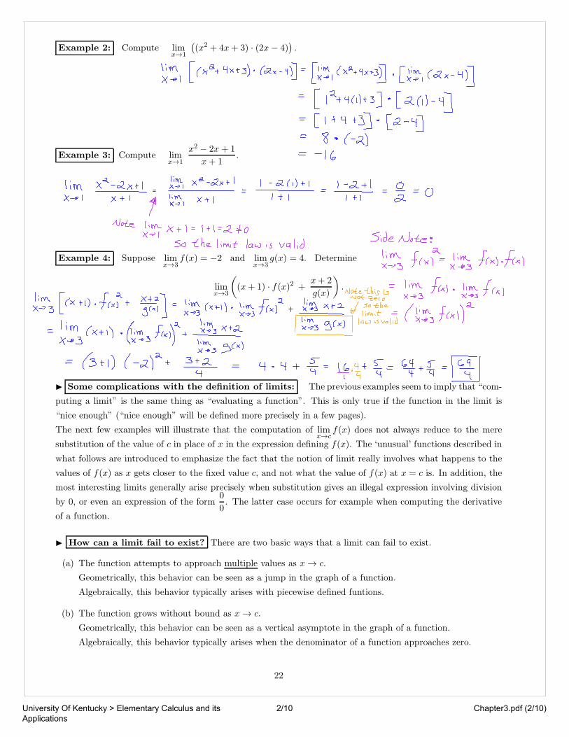
Example 2: Compute limx→1

!

(x2 + 4x+ 3) · (2x− 4)"

.

Example 3: Compute limx→1

x2 − 2x+ 1

x+ 1.

Example 4: Suppose limx→3

f(x) = −2 and limx→3

g(x) = 4. Determine

limx→3

#

(x+ 1) · f(x)2 +x+ 2

g(x)

$

.

! Some complications with the definition of limits: The previous examples seem to imply that “com-

puting a limit” is the same thing as “evaluating a function”. This is only true if the function in the limit is

“nice enough” (“nice enough” will be defined more precisely in a few pages).

The next few examples will illustrate that the computation of limx→c

f(x) does not always reduce to the mere

substitution of the value of c in place of x in the expression defining f(x). The ‘unusual’ functions described in

what follows are introduced to emphasize the fact that the notion of limit really involves what happens to the

values of f(x) as x gets closer to the fixed value c, and not what the value of f(x) at x = c is. In addition, the

most interesting limits generally arise precisely when substitution gives an illegal expression involving division

by 0, or even an expression of the form0

0. The latter case occurs for example when computing the derivative

of a function.

! How can a limit fail to exist? There are two basic ways that a limit can fail to exist.

(a) The function attempts to approach multiple values as x → c.

Geometrically, this behavior can be seen as a jump in the graph of a function.

Algebraically, this behavior typically arises with piecewise defined funtions.

(b) The function grows without bound as x → c.

Geometrically, this behavior can be seen as a vertical asymptote in the graph of a function.

Algebraically, this behavior typically arises when the denominator of a function approaches zero.

22


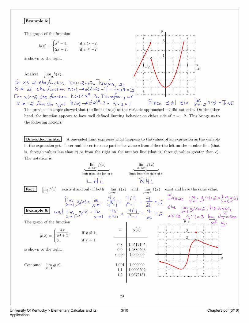
Example 5:

The graph of the function

h(x) =

{

x2 − 3, if x > −2;

2x+ 7, if x ≤ −2

is shown to the right.

Analyze limx→−2

h(x).

x

y

−2

1

3

The previous example showed that the limit of h(x) as the variable approached −2 did not exist. On the other

hand, the function appears to have well defined limiting behavior on either side of x = −2. This brings us to

the following notions:

One-sided limits: A one-sided limit expresses what happens to the values of an expression as the variable

in the expression gets closer and closer to some particular value c from either the left on the number line (that

is, through values less than c) or from the right on the number line (that is, through values greater than c).

The notation is:

limx→c−

f(x)︸︷︷︸

limit from the left of c

limx→c+

f(x)︸︷︷︸

limit from the right of c

Fact: limx→c

f(x) exists if and only if both limx→c−

f(x) and limx→c+

f(x) exist and have the same value.

Example 6:

The graph of the function

g(x) =

4x

x2 + 1, if x #= 1;

3, if x = 1.

is shown to the right.

Compute limx→1

g(x).

x g(x)

0.8 1.95121950.9 1.98895030.999 1.999999

1.001 1.9999991.1 1.99095021.2 1.9672131

x

y

1

2

3

23


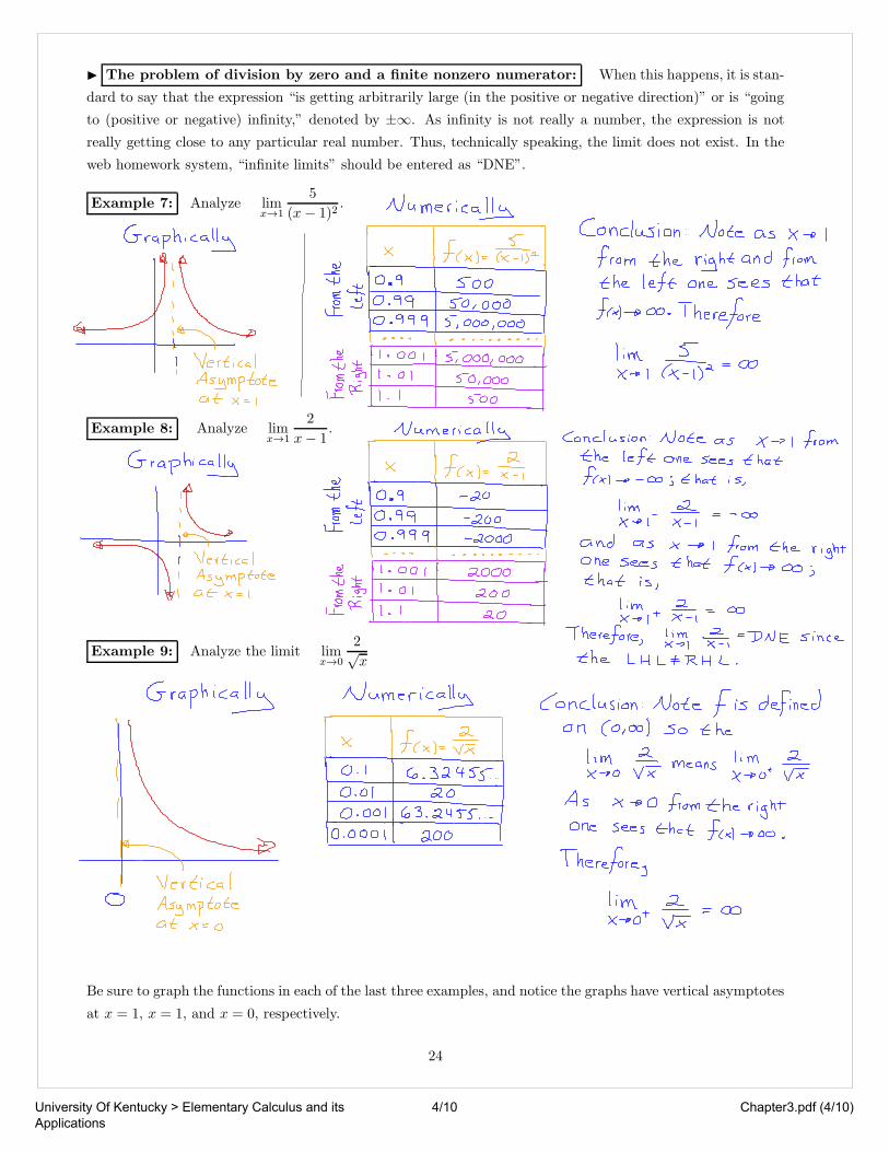
! The problem of division by zero and a finite nonzero numerator: When this happens, it is stan-

dard to say that the expression “is getting arbitrarily large (in the positive or negative direction)” or is “going

to (positive or negative) infinity,” denoted by ±∞. As infinity is not really a number, the expression is not

really getting close to any particular real number. Thus, technically speaking, the limit does not exist. In the

web homework system, “infinite limits” should be entered as “DNE”.

Example 7: Analyze limx→1

5

(x− 1)2.

Example 8: Analyze limx→1

2

x− 1.

Example 9: Analyze the limit limx→0

2√x

Be sure to graph the functions in each of the last three examples, and notice the graphs have vertical asymptotes

at x = 1, x = 1, and x = 0, respectively.

24


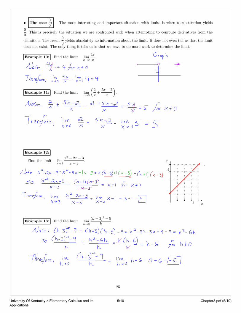
! The case0

0: The most interesting and important situation with limits is when a substitution yields

0

0. This is precisely the situation we are confronted with when attempting to compute derivatives from the

definition. The result0

0yields absolutely no information about the limit. It does not even tell us that the limit

does not exist. The only thing it tells us is that we have to do more work to determine the limit.

Example 10: Find the limit limx→0

4x

x.

Example 11: Find the limit limx→0

!2

x+

5x− 2

x

"

.

Example 12:

Find the limit limx→3

x2 − 2x− 3

x− 3.

x

y

3

4

Example 13: Find the limit limh→0

(h− 3)2 − 9

h.

25


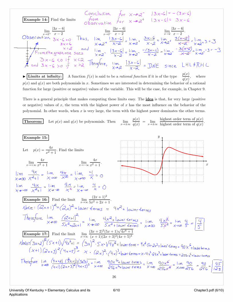
Example 14: Find the limits

limx→2+

|3x− 6|x− 2

limx→2−

|3x− 6|x− 2

limx→2

|3x− 6|x− 2

.

! Limits at infinity: A function f(x) is said to be a rational function if it is of the typep(x)

q(x), where

p(x) and q(x) are both polynomials in x. Sometimes we are interested in determining the behavior of a rational

function for large (positive or negative) values of the variable. This will be the case, for example, in Chapter 9.

There is a general principle that makes computing these limits easy. The idea is that, for very large (positive

or negative) values of x, the term with the highest power of x has the most influence on the behavior of the

polynomial. In other words, when x is very large, the term with the highest power dominates the other terms.

Theorem: Let p(x) and q(x) be polynomials. Then limx→±∞

p(x)

q(x)= lim

x→±∞

highest order term of p(x)

highest order term of q(x).

Example 15:

Let p(x) =4x

x2 + 1. Find the limits

limx→+∞

4x

x2 + 1lim

x→−∞

4x

x2 + 1. x

y

Example 16: Find the limit limx→∞

(2x+ 1)2

5x2 + 2x+ 1.

Example 17: Find the limit limx→∞

(3x+ 2)2(5x+ 1)√4x6 + 1

(x+ 1)(2x + 3)2(4x+ 5)3

26


! Continuity and differentiability:

We first give a brief, non-rigorous and intuitive explanation of two fundamental notions in Calculus whose

definitions involve limits. We then discuss how these two notions relate to each other.

Definition of continuity: A function f is continuous at a point x = c if

limx→c

f(x) = f(c).

A function f is continuous on an interval if it is continuous at every point of that interval.

Note: Geometrically, this means that the graph of f has no holes, jumps, or gaps at any point in the

domain of f . Thus you can draw the graph of f from one end of the interval to the other without lifting your

pencil off the paper.

Analytically, this means the value of the function at x = c can be recovered if one knows the values of f(x) for

near x = c. In other words, the values of a continuous function cannot change abruptly.

Fact: If f and g are continuous functions at c then

kf(x), f(x) + g(x), f(x) · g(x) andf(x)

g(x), where g(c) != 0, are continuous at c.

↑constant

Examples: Many of the standard algebraic functions are continuous.

• Polynomials are continuous at every point.

• Rational functions are continuous at every point in their domain. (i.e., rational functions are continuous

away from zeros of their denominators)

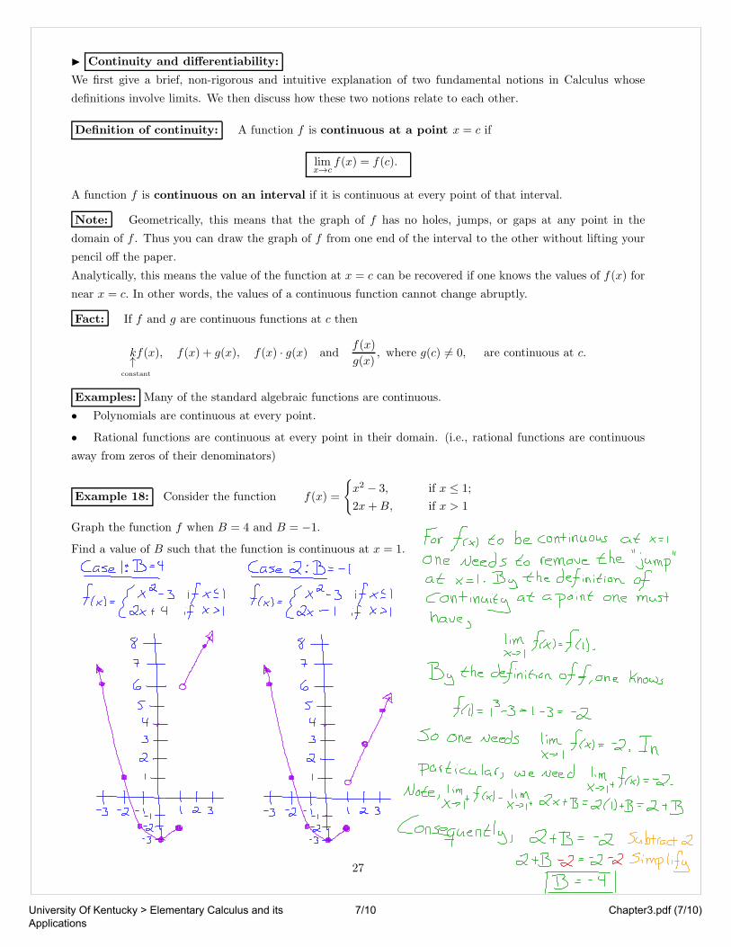
Example 18: Consider the function f(x) =

!

x2 − 3, if x ≤ 1;

2x+B, if x > 1

Graph the function f when B = 4 and B = −1.

Find a value of B such that the function is continuous at x = 1.

27


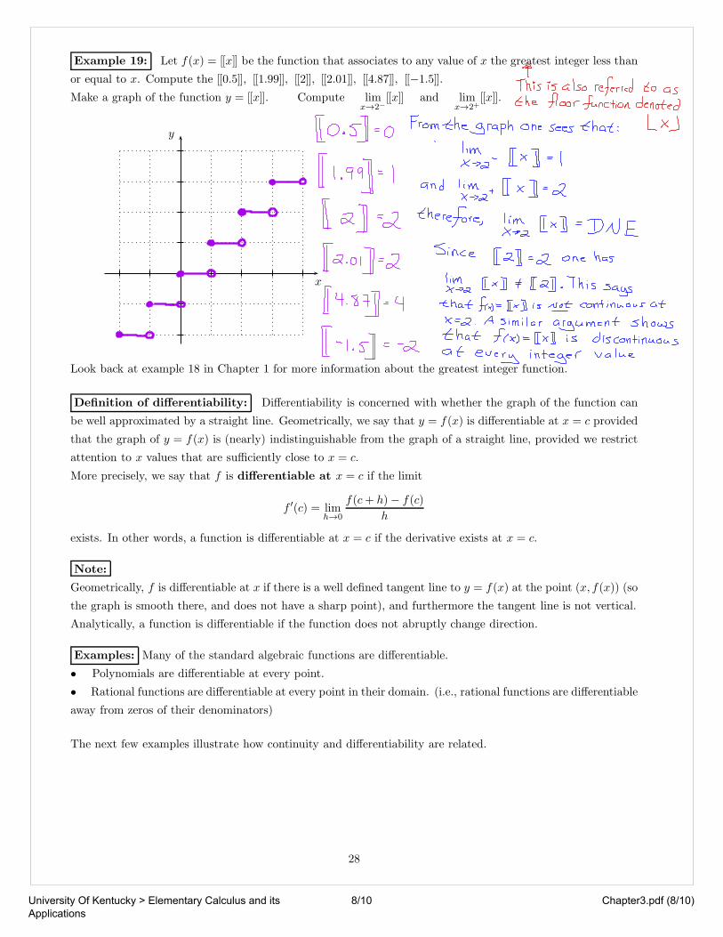
Example 19: Let f(x) = [[x]] be the function that associates to any value of x the greatest integer less than

or equal to x. Compute the [[0.5]], [[1.99]], [[2]], [[2.01]], [[4.87]], [[−1.5]].

Make a graph of the function y = [[x]]. Compute limx→2−

[[x]] and limx→2+

[[x]].

x

y

Look back at example 18 in Chapter 1 for more information about the greatest integer function.

Definition of differentiability: Differentiability is concerned with whether the graph of the function can

be well approximated by a straight line. Geometrically, we say that y = f(x) is differentiable at x = c provided

that the graph of y = f(x) is (nearly) indistinguishable from the graph of a straight line, provided we restrict

attention to x values that are sufficiently close to x = c.

More precisely, we say that f is differentiable at x = c if the limit

f ′(c) = limh→0

f(c+ h)− f(c)

h

exists. In other words, a function is differentiable at x = c if the derivative exists at x = c.

Note:

Geometrically, f is differentiable at x if there is a well defined tangent line to y = f(x) at the point (x, f(x)) (so

the graph is smooth there, and does not have a sharp point), and furthermore the tangent line is not vertical.

Analytically, a function is differentiable if the function does not abruptly change direction.

Examples: Many of the standard algebraic functions are differentiable.

• Polynomials are differentiable at every point.

• Rational functions are differentiable at every point in their domain. (i.e., rational functions are differentiable

away from zeros of their denominators)

The next few examples illustrate how continuity and differentiability are related.

28


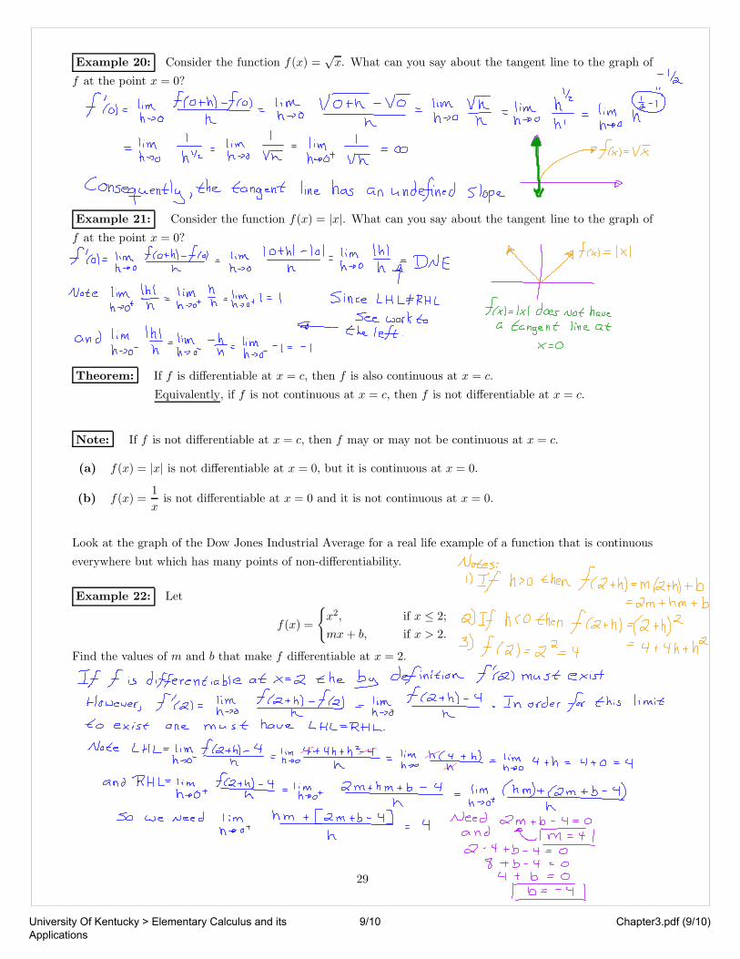
Example 20: Consider the function f(x) =√x. What can you say about the tangent line to the graph of

f at the point x = 0?

Example 21: Consider the function f(x) = |x|. What can you say about the tangent line to the graph of

f at the point x = 0?

Theorem: If f is differentiable at x = c, then f is also continuous at x = c.

Equivalently, if f is not continuous at x = c, then f is not differentiable at x = c.

Note: If f is not differentiable at x = c, then f may or may not be continuous at x = c.

(a) f(x) = |x| is not differentiable at x = 0, but it is continuous at x = 0.

(b) f(x) =1

xis not differentiable at x = 0 and it is not continuous at x = 0.

Look at the graph of the Dow Jones Industrial Average for a real life example of a function that is continuous

everywhere but which has many points of non-differentiability.

Example 22: Let

f(x) =

!

x2, if x ≤ 2;

mx+ b, if x > 2.

Find the values of m and b that make f differentiable at x = 2.

29


30

MA123, Chapter 3: The idea of limits (pp. 47-67, Gootman)

Documents