Ma Dissertation

SOLUTIONS OF ESHELBY-TYPE INCLUSION PROBLEMS AND A

RELATED HOMOGENIZATION METHOD BASED ON A

SIMPLIFIED STRAIN GRADIENT ELASTICITY THEORY

A Dissertation

by

HEMEI MA

Submitted to the Office of Graduate Studies of Texas A&M University

in partial fulfillment of the requirements for the degree of

DOCTOR OF PHILOSOPHY

May 2010

Major Subject: Mechanical Engineering

SOLUTIONS OF ESHELBY-TYPE INCLUSION PROBLEMS AND A

RELATED HOMOGENIZATION METHOD BASED ON A

SIMPLIFIED STRAIN GRADIENT ELASTICITY THEORY

A Dissertation

by

HEMEI MA

Submitted to the Office of Graduate Studies of Texas A&M University

in partial fulfillment of the requirements for the degree of

DOCTOR OF PHILOSOPHY

Approved by:

Chair of Committee, Xin-Lin Gao Committee Members, Anastasia Muliana J. N. Reddy Jay Walton Head of Department, Dennis O’Neal

May 2010

Major Subject: Mechanical Engineering

iii

ABSTRACT

Solutions of Eshelby-Type Inclusion Problems and a Related Homogenization Method

Based on a Simplified Strain Gradient Elasticity Theory. (May 2010)

Hemei Ma, B.Sc., Tongji University, Shanghai, China;

M.Sc., Tongji University, Shanghai, China

Chair of Advisory Committee: Dr. Xin-Lin Gao

Eshelby-type inclusion problems of an infinite or a finite homogeneous isotropic

elastic body containing an arbitrary-shape inclusion prescribed with an eigenstrain and an

eigenstrain gradient are analytically solved. The solutions are based on a simplified strain

gradient elasticity theory (SSGET) that includes one material length scale parameter in

addition to two classical elastic constants.

For the infinite-domain inclusion problem, the Eshelby tensor is derived in a

general form by using the Green’s function in the SSGET. This Eshelby tensor captures

the inclusion size effect and recovers the classical Eshelby tensor when the strain gradient

effect is ignored. By applying the general form, the explicit expressions of the Eshelby

tensor for the special cases of a spherical inclusion, a cylindrical inclusion of infinite

length and an ellipsoidal inclusion are obtained. Also, the volume average of the new

Eshelby tensor over the inclusion in each case is analytically derived. It is quantitatively

shown that the new Eshelby tensor and its average can explain the inclusion size effect,

unlike its counterpart based on classical elasticity.

To solve the finite-domain inclusion problem, an extended Betti’s reciprocal

iv

theorem and an extended Somigliana’s identity based on the SSGET are proposed and

utilized. The solution for the disturbed displacement field incorporates the boundary

effect and recovers that for the infinite-domain inclusion problem. The problem of a

spherical inclusion embedded concentrically in a finite spherical body is analytically

solved by applying the general solution, with the Eshelby tensor and its volume average

obtained in closed forms. It is demonstrated through numerical results that the newly

obtained Eshelby tensor can capture the inclusion size and boundary effects, unlike

existing ones.

Finally, a homogenization method is developed to predict the effective elastic

properties of a heterogeneous material using the SSGET. An effective elastic stiffness

tensor is analytically derived for the heterogeneous material by applying the Mori-Tanaka

and Eshelby’s equivalent inclusion methods. This tensor depends on the inhomogeneity

size, unlike what is predicted by existing homogenization methods based on classical

elasticity. Numerical results for a two-phase composite reveal that the composite

becomes stiffer when the inhomogeneities get smaller.

v

ACKNOWLEDGEMENTS

I would like to gratefully thank my advisor, Professor Xin-Lin Gao, for his

support, guidance, patience and encouragement during my graduate studies at Texas

A&M University. He has demonstrated to me what makes a great researcher: dedication,

diligence, persistence, commitment to excellence, and honor. Without him, this

dissertation work would not have been possible.

I am very thankful to my other committee members, Professor J.N. Reddy,

Professor Jay Walton, Professor Anastasia Muliana and Professor Steve Suh, for their

time and help. I have benefitted greatly from their comments and advice. I also thank

everyone in Professor Gao’s research group for helping me over the years.

Especially, I am eternally grateful to my parents, my husband and my sister for

their unconditional and selfless love. I am so blessed to have their full support during my

graduate studies and in my daily life.

Finally, I thank my Lord, Jesus Christ, who helps me to overcome all frustrations.

He gives me hope, faith, love and compassion.

vi

TABLE OF CONTENTS

Page

ABSTRACT .................................................................................................................. iii

ACKNOWLEDGEMENTS .......................................................................................... v

TABLE OF CONTENTS .............................................................................................. vi

LIST OF FIGURES ...................................................................................................... ix

CHAPTER

I INTRODUCTION ............................................................................................. 1 1 4 5

1.1 Background ............................................................................................ 1.2 Motivation….. ......................................................................................... 1.3 Organization ............................................................................................

II GREEN’S FUNCTION AND ESHELBY TENSOR BASED ON A SIMPLIFED STRAIN GRADIENT ELASTICITY THEORY .........................

8 8 9 13 18 23

2.1 Introduction ............................................................................................ 2.2 Simplified Strain Gradient Elasticity Theory (SSGET) .......................... 2.3 Green’s Function Based on SSGET ........................................................ 2.4 Eshelby Tensor and Eshelby-like Tensor ................................................ 2.5 Conclusion ...............................................................................................

III ESHELBY TENSOR FOR A SPHERICAL INCLUSION ............................... 25

25 25 34 39

3.1 Introduction ............................................................................................ 3.2 Eshelby Tensor for a Spherical Inclusion ................................................ 3.3 Numerical Results .................................................................................... 3.4 Summary ..................................................................................................

IV ESHELBY TENSOR FOR A PLANE STRAIN CYLINDRICAL INCLUSION ......................................................................................................

40

40 40 53 56

4.1 Introduction ............................................................................................ 4.2 Eshelby Tensor for a Cylindrical Inclusion ............................................. 4.3 Numerical Results .................................................................................... 4.4 Summary .................................................................................................

vii

CHAPTER Page

V STRAIN GRADIENT SOLUTION FOR ESHELBY’S ELLIPSOIDAL INCLUSION PROBLEM .................................................................................

58

58 58 71 75

5.1 Introduction ............................................................................................. 5.2 Ellipsoidal Inclusion ................................................................................ 5.3 Numerical Results .................................................................................... 5.4 Summary ..................................................................................................

VI SOLUTION OF AN ESHELBY-TYPE INCLUSION PROBLEM WITH A BOUNDED DOMAIN AND THE ESHELBY TENSOR FOR A SPHERICAL INCLUSION IN A FINITE SPHERICAL MATRIX .................

77

6.1 Introduction ............................................................................................. 6.2 Strain Gradient Solution of Eshelby’s Inclusion Problem in a Finite Domain…. ............................................................................................... 6.2.1 Extended Betti’s reciprocal theorem ........................................ 6.2.2 Extended Somigliana’s identity and solution of Eshelby’s inclusion problem in a finite domain ........................................ 6.3 Eshelby Tensor for a Finite-Domain Spherical Inclusion Problem ......... 6.3.1 Position-dependent Eshelby tensor .......................................... 6.3.2 Volume averaged Eshelby tensor ............................................ 6.4 Numerical Results .................................................................................... 6.5 Summary ..................................................................................................

77

79 79

81 89 89 98 99 103

VII A HOMOGENIZATION METHOD BASED ON THE ESHELBY TENSOR …........................................................................................................

105

105 106 113 116 122

7.1 Introduction ............................................................................................. 7.2 Homogenization Scheme Based on the Strain Energy Equivalence ....... 7.3 New Homogenization Method Based on the SSGET .............................. 7.4 Numerical Results .................................................................................... 7.5 Summary ..................................................................................................

VIII SUMMARY ....................................................................................................... 124

REFERENCES ............................................................................................................. 128

APPENDIX A ............................................................................................................... 136

APPENDIX B ............................................................................................................... 137

viii

Page

APPENDIX C ............................................................................................................... 139

APPENDIX D ............................................................................................................... 141

APPENDIX E ............................................................................................................... 144

APPENDIX F................................................................................................................ 149

APPENDIX G ............................................................................................................... 151

APPENDIX H ............................................................................................................... 153

APPENDIX I ................................................................................................................ 155

VITA ............................................................................................................................ 156

ix

LIST OF FIGURES

FIGURE Page

1.1 Macroscopic composite material and its microscopic structures ….. .......... 2

1.2a

Inclusion problem .........................................................................................

3

1.2b Inhomogeneity problem ................................................................................

3

3.1 1111S along a radial direction of the spherical inclusion ............................... 36

3.2 1212S along a radial direction of the spherical inclusion….. ......................... 37

3.3 2222S along a radial direction of the spherical inclusion….. ......................... 37

3.4 V1111S varying with the inclusion radius….. ............................................... 38

4.1 1111S along a radial direction of the cylindrical inclusion….. ....................... 54

4.2 1212S along a radial direction of the cylindrical inclusion….. ....................... 55

4.3 V1111S varying with the inclusion radius….. ............................................... 56

5.1 Ellipsoidal inclusion problem….. ................................................................. 59

5.2 3333S along the x3 axis of the ellipsoidal inclusion….. .................................. 72

5.3 V3333S changing with the inclusion size for different aspect ratio

values….. ......................................................................................................

74

5.4 Comparison of V3333S and

V

,3333

INCS ….. ......................................................... 74

6.1 Inclusion in a finite elastic body….. ............................................................. 81

6.2 Spherical inclusion in a finite spherical elastic body….. ............................. 89

6.3 Locations of x (∈ Ω) and y (∈ ∂Ω).….. ........................................................ 94

6.4 FIS ,1111 along a radical direction of the inclusion for the matrix with

different sizes….. ..........................................................................................

100

x

FIGURE Page

6.5 V

,1111

FIS varying with the inclusion size at different inclusion volume

fractions….. ..................................................................................................

102

7.1 Heterogeneous RVE….. ............................................................................... 107

7.2 Effective Young’s modulus of a composite with spherical inhomogeneities….. ......................................................................................

119

7.3 In-plane Young’s modulus of a composite with cylindrical inhomogeneities….. ......................................................................................

120

7.4 Effective HE11 of a composite with ellipsoidal inhomogeneities….................

121

7.5 Effective HE33 of a composite with ellipsoidal inhomogeneities….................

122

1

CHAPTER I

INTRODUCION

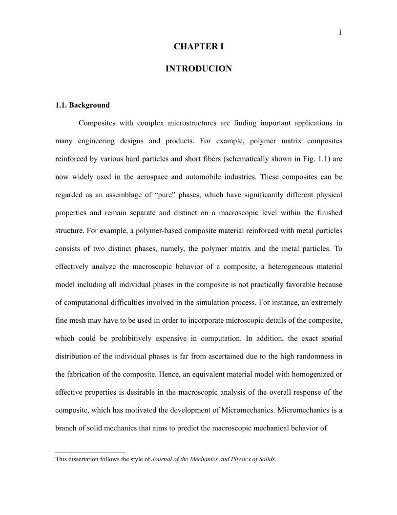
1.1. Background

Composites with complex microstructures are finding important applications in

many engineering designs and products. For example, polymer matrix composites

reinforced by various hard particles and short fibers (schematically shown in Fig. 1.1) are

now widely used in the aerospace and automobile industries. These composites can be

regarded as an assemblage of “pure” phases, which have significantly different physical

properties and remain separate and distinct on a macroscopic level within the finished

structure. For example, a polymer-based composite material reinforced with metal particles

consists of two distinct phases, namely, the polymer matrix and the metal particles. To

effectively analyze the macroscopic behavior of a composite, a heterogeneous material

model including all individual phases in the composite is not practically favorable because

of computational difficulties involved in the simulation process. For instance, an extremely

fine mesh may have to be used in order to incorporate microscopic details of the composite,

which could be prohibitively expensive in computation. In addition, the exact spatial

distribution of the individual phases is far from ascertained due to the high randomness in

the fabrication of the composite. Hence, an equivalent material model with homogenized or

effective properties is desirable in the macroscopic analysis of the overall response of the

composite, which has motivated the development of Micromechanics. Micromechanics is a

branch of solid mechanics that aims to predict the macroscopic mechanical behavior of

This dissertation follows the style of Journal of the Mechanics and Physics of Solids.

2

materials based on the understanding of their microstructures (e.g., Mura, 1987; Qu and

Cherkaoui, 2006; Nemat-Nasser and Hori, 1999; Li and Wang, 2008). It studies composites

or heterogeneous materials by incorporating microstructures of individual phases that

constitute these materials, and uses suitable homogenization methods to determine the

effective properties that can be applied directly in the macroscale analysis.

Fig.1.1. Macroscopic composite material and its microscopic structures.

The beginning of micromechanics may be traced back to Eshelby’s seminal study in

the 1950s (Eshelby, 1957, 1959). On the microscopic scale, the problem of inhomogeneities,

whose material properties are different from their surrounding matrix, is encountered. This

problem was not analytically solved until Eshelby proposed an eigenstrain method for an

inclusion problem, which can be used to simulate the inhomogeneity problem. According to

Eshelby’s original work, an inclusion is defined as a subdomain I in an infinite domain

, where a stress-free eigenstrain *ε is prescribed in the inclusion I and vanishes outside

(see Fig. 1.2a). The material property, denoted by MC in Fig. 1.2a, is the same in I and

I . In a similar way, an inhomogeneity is defined as a subdomain H in an infinite

domain (see Fig.1.2b), where the material properties in H and in H , denoted

respectively by FC and MC in Fig.1.2b, are different. From the above definitions, it is clear

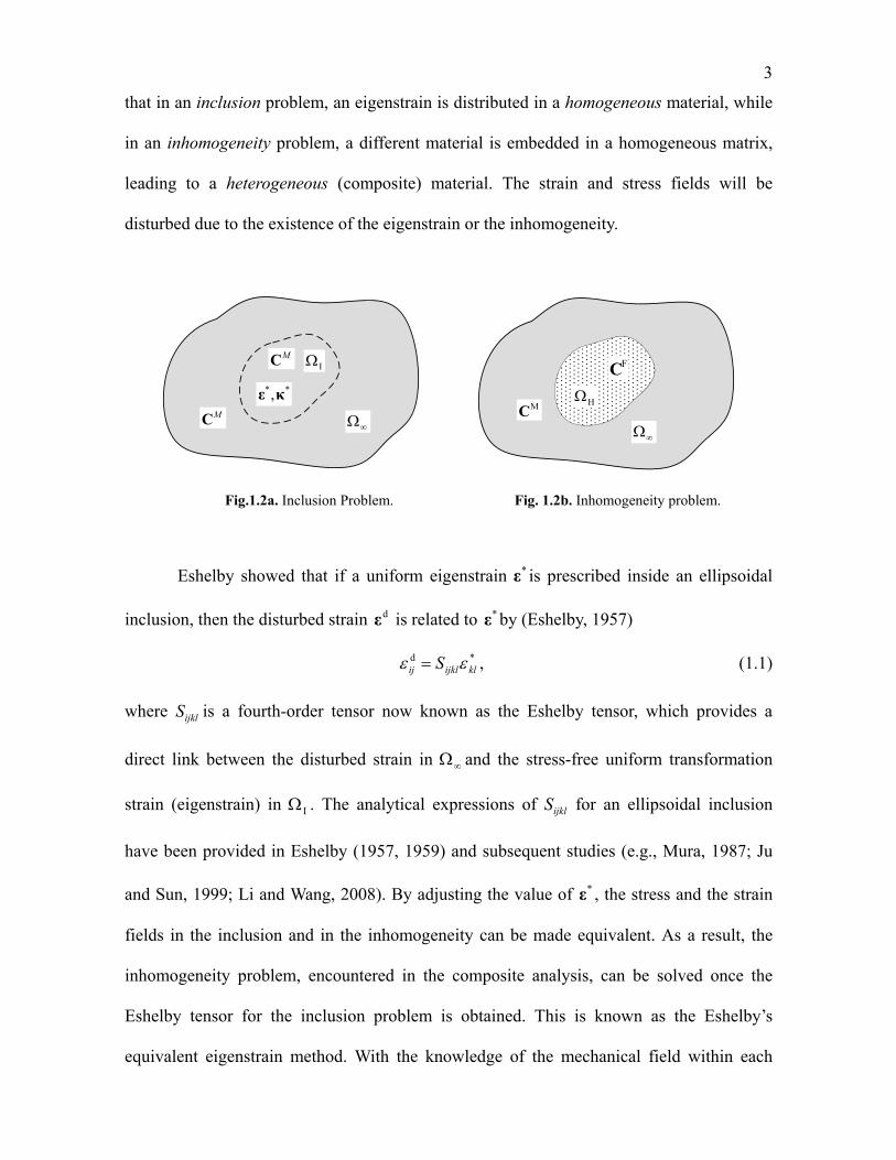
3

that in an inclusion problem, an eigenstrain is distributed in a homogeneous material, while

in an inhomogeneity problem, a different material is embedded in a homogeneous matrix,

leading to a heterogeneous (composite) material. The strain and stress fields will be

disturbed due to the existence of the eigenstrain or the inhomogeneity.

MC

FC**,κε

I

MC

MC

H

Fig.1.2a. Inclusion Problem. Fig. 1.2b. Inhomogeneity problem.

Eshelby showed that if a uniform eigenstrain *ε is prescribed inside an ellipsoidal

inclusion, then the disturbed strain dε is related to *ε by (Eshelby, 1957)

*dklijklij S , (1.1)

where ijklS is a fourth-order tensor now known as the Eshelby tensor, which provides a

direct link between the disturbed strain in and the stress-free uniform transformation

strain (eigenstrain) in I . The analytical expressions of ijklS for an ellipsoidal inclusion

have been provided in Eshelby (1957, 1959) and subsequent studies (e.g., Mura, 1987; Ju

and Sun, 1999; Li and Wang, 2008). By adjusting the value of *ε , the stress and the strain

fields in the inclusion and in the inhomogeneity can be made equivalent. As a result, the

inhomogeneity problem, encountered in the composite analysis, can be solved once the

Eshelby tensor for the inclusion problem is obtained. This is known as the Eshelby’s

equivalent eigenstrain method. With the knowledge of the mechanical field within each

4

constituent of the heterogeneous material, it is now possible to determine the overall or

effective mechanical properties based on some averaging theorems. Clearly, the Eshelby

tensor ijklS plays a key role in such homogenization analysis, and the development of new

homogenization methods will hinge on the availability of new expressions of ijklS .

1.2. Motivation

Despite the significance of the Eshelby tensor ijklS in Micromechanics, it is deduced

by Eshelby and most subsequent researchers based on classical elasticity and depends only

on the elastic constants and the inclusion shape (e.g., the aspect ratios for an ellipsoidal

inclusion). As a result, the Eshelby tensor and the subsequent homogenization methods

cannot capture the size effect exhibited by particle-matrix composites at the micro- or nano-

scale (e.g., Vollenberg and Heikens, 1989; Vollenberg, et al., 1989; Lloyd, 1994; Kouzeli

and Mortensen, 2002). This has motivated the studies on Eshelby-type inclusion problems

using higher-order elasticity theories, which, unlike classical elasticity, contain

microstructure-dependent material length scale parameters and are therefore capable of

explaining the size effect.

The higher-order elasticity theories that have been used in studying the Eshelby

inclusion problems include a micropolar theory (Cheng and He, 1995, 1997; Ma and Hu,

2006), a microstretch theory (Kiris and Inan, 2006; Ma and Hu, 2007), a modified couple

stress theory (Zheng and Zhao, 2004), and a strain gradient elasticity theory (Zhang and

Sharma, 2005). However, most of the higher-order elasticity theories used in these studies

involve at least four elastic constants, with two or more being the material length scale

parameters. Due to the difficulties in determining these microstructure-dependent length

scale parameters (e.g., Lakes, 1995; Lam et al., 2003; Maranganti and Sharma, 2007) and in

5

dealing with the fourth-order Eshelby tensor, it is very desirable to study the Eshelby

inclusion problem using a higher-order elasticity theory containing only one material length

scale parameter in addition to the two classical elastic constants. Among the afore-

mentioned works, the one reported in Zheng and Zhao (2004) appears to be the only study

that involves just one additional length scale parameter, which is based on a couple stress

theory modified from the classical couple stress theory (Koiter, 1964) that contains four

elastic constants in the constitutive equations but three in the displacement-equations of

equilibrium. There is still a lack of studies on the Eshelby-type inclusion problems based on

strain gradient elasticity theories involving only one additional elastic constant. The

objective of this dissertation is therefore to provide a systematic study of various Eshelby-

type inclusion problems involving a spherical, cylindrical or ellipsoidal inclusion embedded

in an infinite or a finite homogeneous isotropic elastic body, applying a simpler one-length-

scale-parameter strain gradient theory. It will be based on a simplified strain gradient theory

(SSGET) elaborated by Gao and Park (2007), which involves only one material length

parameter in addition to two classical elastic constants. The resulting non-classical Eshelby

tensors based on the SSGET will then be utilized to develop new homogenization methods

for analyzing heterogeneous composites.

1.3. Organization

The rest of this dissertation is organized as follows.

In Chapter II, the Green’s function in the SSGET is first obtained in terms of

elementary functions by applying Fourier transforms, which reduces to the Green’s function

in classical elasticity when the strain gradient effect is not considered. The Eshelby tensor is

then derived in a general form for an inclusion of arbitrary shape, which consists of a

6

classical part and a gradient part. The former depends on two classical elastic constants only,

while the latter depends on the length scale parameter additionally, thereby enabling the

interpretation of the size effect.

In Chapter III and Chapter IV, the explicit expressions of the Eshelby tensors for a

spherical and for a cylindrical inclusion are obtained, respectively, by applying the general

form of the Eshelby tenor derived in Chapter II. Both of the non-classical Eshelby tensors

varies with positions even inside the inclusions and captures the inclusion-size dependence,

unlike the classical Eshelby tensors. The volume averages of these newly derived Eshelby

tensors over the spherical and the cylindrical inclusions are obtained in closed forms, to

facilitate the further homogenization analyses of particle-reinforced and fiber-reinforced

composites.

In Chaper 5, the problem of an ellipsoidal inclusion (with three distinct semi-axes)

in an infinite homogeneous isotropic elastic material is analytically solved by using the

general form of the Eshelby tensor in the SSGET. Analytical expressions for the Eshelby

tensor are derived for both the interior and exterior cases in terms of two line integrals with

an unbounded upper limit and two surface integrals over a unit sphere. The Eshelby tensors

for the spherical and cylindrical inclusion problems based on the SSGET are included in the

current Eshelby tensor as two limiting cases. The volume average of the new Eshelby

tensor over the ellipsoidal inclusion needed in homogenization analyses is also analytically

obtained in this chapter.

In Chapter VI, a solution for the Eshelby-type inclusion problem of a finite

homogeneous isotropic elastic body containing an inclusion prescribed with a uniform

eigenstrain and a uniform eigenstrain gradient is derived in a general form using the SSGET.

An extended Betti’s reciprocal theorem and an extended Somigliana’s identity based on the

7

SSGET are proposed and utilized to solve the finite-domain inclusion problem. The

solution for the disturbed displacement field is expressed in terms of the Green’s function

for an infinite three-dimensional elastic body in the SSGET. It contains a volume integral

term and a surface integral term. The former is the same as that for the infinite-domain

inclusion problem based on the SSGET, while the latter represents the boundary effect. The

solution reduces to that of the infinite-domain inclusion problem when the boundary effect

is not considered. The problem of a spherical inclusion embedded concentrically in a finite

spherical elastic body is analytically solved by applying the general solution, with the

Eshelby tensor and its volume average obtained in closed forms.

A homogenization method is developed in Chapter VII to predict the effective

elastic properties of a heterogeneous material in the framework of the SSGET. At the

macroscopic scale, the heterogeneous material is modeled as a homogeneous strain-

gradient medium whose behavior can be characterized by the constitutive relations in the

SSGET. The effective elastic properties of the heterogeneous material are found to be

dependent not only on the volume fractions and shapes of the inhomogeneities but also on

the inhomogeneity sizes, unlike what is predicted by the homogenization method based on

classical elasticity. The effective elastic stiffness tensor is analytically obtained by using the

Mori-Tanaka method and Eshelby’s equivalent inclusion method.

8

CHAPTER II

GREEN’S FUNCTION AND ESHELBY

TENSOR BASED ON A SIMPLIFIED STRAIN

GRADIENT ELASTICITY THEORY

2.1. Introduction

In this chapter, a simplified strain gradient elasticity theory (SSGET) involving only

one additional material length scale parameter (Altan and Aifantis, 1997; Gao and Park,

2007) is used to analytically solve the Eshelby-type problem of an infinite homogeneous

isotropic elastic medium containing an inclusion of arbitrary shape. A variationally

consistent formulation of the SSGET was provided in Gao and Park (2007). This simplified

strain gradient elasticity theory has been applied to solve a number of problems (e.g.,

Lazopoulos, 2004; Li et al., 2004; Gao and Park, 2007; Gao et al., 2009).

The rest of this chapter is organized as follows. In Section 2.2, the simplified strain

gradient elasticity theory (SSGET) is fist reviewed. It is followed by Section 2.3 where a

three-dimensional (3-D) Green’s function in the SSGET is obtained from directly solving

the governing equations using Fourier transforms. Based on this Green’s function obtained,

the Eshelby tensor is derived in Section 2.4 in a general form for a 3-D inclusion of

arbitrary shape, which consists of a classical part and a gradient part. The former contains

only one classical elastic constant (Poisson’s ratio), while the latter includes the length scale

parameter additionally. This chapter concludes with a summary in Section 2.5.

9

2.2. Simplified Strain Gradient Elasticity Theory (SSGET)

As reviewed in Gao and Ma (2010a), the SSGET is the simplest strain gradient

elasticity theory evolving from Mindlin’s pioneering work (Mindlin, 1964, 1965; Mindlin

and Eshel, 1968). It is also known as the first gradient elasticity theory of Helmholtz type

(e.g., Lazar et al., 2005) and the dipolar gradient elasticity theory (e.g., Georgiadis et al.,

2004). The SSGET has been well studied and successfully used to solve a number of

important problems on dislocations (e.g., Lazar and Maugin, 2005), cracking (e.g., Altan

and Aifantis, 1992; Gourgiotis and Georgiadis, 2009), wave dispersion (e.g., Georgiadis et

al., 2004), inclusions (Gao and Ma, 2009, 2010a, 2010b; Ma and Gao, 2009), beams (e.g.,

Giannakopoulos and Stamoulis, 2007), plates (e.g., Lazopoulos, 2004), and thick-walled

shells (Gao and Park, 2007; Gao et al., 2009).

However, for a better understanding of this relatively recent SSGET, further

elaborations on the aspects of the theory interpretation and length scale parameter

determination are still warranted. There has been a slow embracement of strain gradient

elasticity and plasticity theories, as indicated earlier by Fleck and Hutchinson (1997) for

strain gradient elasticity theories and very recently by Evans and Hutchinson (2009) for

strain gradient plasticity theories. One reason for this slow embracement is the lack of

clarity in the theory interpretation, and another is the ambiguity in determining length scale

parameters through curve fitting (Evans and Hutchinson, 2009). These apply to the SSGET

and therefore will be discussed further below.

As stated in Gao and Park (2007), elements of the SSGET were first suggested by

Altan and Aifantis (1992, 1997) by simplifying Mindlin’s first strain gradient theory in

linear elasticity (Mindlin and Eshel, 1968) without derivations. The strain energy density

function, w, employed by Mindlin and Eshel (1968) for an isotropic linearly elastic material

10

has the general form:

,2

1

),(

,,5,,4,,3,,2,,1

,

ikjkijkijkijkjjkiijkjkiikikjijijijjjii

kijij

ccccc

ww

(2.1)

where εij is the infinitesimal strain, and are the Lamé constants in classical elasticity,

and c1–c5 are the five additional material constants (called strain gradient coefficients)

having the dimension of force. By taking

,,2

1,0 43521 ccccccc (2.2)

Eq. (2.1) becomes

,2

1

2

1),( ,,,,,

kijkijkjjkiiijijjjiikijij cww (2.3)

where c, as the only remaining strain gradient coefficient, has the dimension of length

squared. Eq. (2.3) can also be written as (Gao and Park, 2007)

,2

1),( , ijkijkijijkijijww (2.4)

where the Cauchy stress τij (energetically conjugated to εij), the double stress ijk

(energetically conjugated to κijk), the infinitesimal strain εij, and the strain gradient κijk are,

respectively, defined by

),2(,2 22ijkijllkmnkijmnijkijijllklijklij μδλLCLμμεδεC

,2

1,

2

1,,,,, ikjjkikijijkijjiij uuuu (2.5a–d)

where ui is the displacement and ij is the Kronecker delta. In Eqs. (2.5a,b), L is the material

length scale parameter (with L2 = c, c being the strain gradient coefficient introduced in Eq.

(2.3)) and Cijkl is the elastic stiffness tensor for isotropic elastic materials given by

11

)( jkiljlikklijijklC . (2.6)

The simplified strain energy density function in Eq. (2.3) was first suggested in

Altan and Aifantis (1997) without reasoning. Following Lazar and Maugin (2005), it can

now be understood that this simplified strain energy density function is physical and

exhibits the symmetry both in ij and ij and in ijk and ijk for the linearly elastic material,

as shown in Eq. (2.4). Based on Eq. (2.3), a variationally consistent formulation of the

SSGET has been provided in Gao and Park (2007), leading to the simultaneous

determination of the governing equations and the complete boundary conditions. However,

the form of the strain energy density function w given in Eq. (2.3) or Eq. (2.1) can be

discussed further next.

Physically, for linearly elastic materials, the dependence of w on

kjikij eeeε , included in Eq. (2.1) arises from the non-local nature of atomic forces,

which was first studied by Kröner (1963), where the connection between the lattice

curvature and the double stress was explored and the necessity of including the strain

gradient effect for some elastic materials was demonstrated. This was pointed out earlier by

Nix and Gao (1998). The mathematical framework that led to Mindlin’s strain energy

density function in Eq. (2.1) was established by Toupin (1962) and Green and Rivlin

(1964a, b).

For plastically deformable materials, the strain gradient effect as reflected in Eq.

(2.1) is associated with geometrically necessary dislocations, which is in addition to the

homogeneous plastic strain arising from statistically stored dislocations (e.g., Ashby, 1970;

Fleck et al., 1994; Nix and Gao, 1998; Gao et al., 1999). As a result, the strain energy

density function given in Eq. (2.1) was adopted by Fleck and Hutchinson (1997) in

12

developing their strain gradient plasticity theory for incompressible materials, where 0ii

and the first, fourth and fifth terms in Eq. (2.1) vanish, thereby leaving only three additional

constants c1, c4 and c5 in the expression of w for the general case. These three constants can

be determined from fitting experimental data obtained in micro-torsion, micro-bending and

micro-indentation tests (e.g., Fleck and Hutchinson, 1997; Shi et al., 2000; Lam et al.,

2003).

The determination of the only material length scale parameter L involved in the

SSGET, which is introduced in Eq. (2.3) through c = L2, has been discussed in a number of

publications. The most recent one is that by Gourgiotis and Georgiadis (2009), where it was

stated that the coefficient c (and thus L) can be estimated from comparing the dispersion

curves of Rayleigh waves obtained using the strain gradient theory based on Eq. (2.3) and

those from lattice dynamics calculations, as was done in Georgiadis et al. (2004). This

approach was also used earlier by Altan and Aifantis (1992). Similar to that in the strain

gradient plasticity theory of Fleck and Hutchinson (1997) for determining c1, c4 and c5

mentioned above, the parameter L can also be estimated by fitting experimental data from

small-scale tests. This has been demonstrated by Giannakopoulos and Stamoulis (2007) by

fitting the strain gradient elasticity based analytical results for the normalized stiffness of a

cantilever beam to the experimental data obtained by Kakunai et al. (1985) using

heterodyne holographic interferometry. Efforts have also been made to estimate L by fitting

the measured data from bending and torsion tests of microstructured solids (including bones

and polymeric foams) that are elastically deformed (Aifantis, 1999, 2003). These reported

methods for determining the material length scale parameter L in the SSGET have been

elaborated by Lakes (1995) together with other methods in a broader context.

As shown in Gao and Park (2007), in the SSGET the equilibrium equations have the

13

form:

0, ijij f , (2.7)

where fi is the body force, and ij is the total stress, which is related to the Cauchy stress

through

,,kijkijij μτσ (2.8)

with the Cauchy stress τij and the double stress ijk given in Eqs. (2.5a–d) in terms of the

displacement ui.

Substituting Eqs. (2.5a–d) and (2.8) into Eq. (2.7) yields the Navier-like

displacement equations of equilibrium in the SSGET as

2, , , , ,

( ) ( ) 0i ij j kk i ij j kk jmmu u L u u f . (2.9)

Clearly, Eq. (2.9) reduces to the Navier equations in classical elasticity when L = 0 (i.e.,

when the strain gradient effect is not considered). Note that the standard index notation,

together with the Einstein summation convention, is used in Eqs. (2.1)–(2.9) and

throughout this dissertation, with each Latin index (subscript) ranging from 1 to 3 and each

Greek index (subscript) ranging from 1 to 2, unless otherwise stated.

2.3. Green’s Function Based on SSGET

The solution of Eq. (2.9) subject to the boundary conditions of ui and their

derivatives vanishing at infinity, provides the fundamental solution and Green’s function in

the SSGET, as will be shown next.

The 3-D Fourier transform of a sufficiently smooth function F(x) and its inverse can

be defined as

14

xxξ xξ deFF i

)()(ˆ , (2.10a)

ξξx xξ deFF i

)(ˆ)2(

1)(

3, (2.10b)

where x is the position vector of a point in the 3-D physical space, ξ is the position vector

of the same point in the Fourier (transformed) space, i is the usual imaginary number with i2

= 1, and )(ˆ ξF is the Fourier transform of F(x).

Suppose that ui are sufficiently differentiable and that ui and their derivatives vanish

at x. Then, applying Eq. (2.10a), the product rule and the divergence theorem gives

).(ˆ)(ˆ),(ˆ)(ˆ,)()(ˆ ,,i ξξξξxxξ xξ

klljiijllkkjiijkii uuuudeuu

(2.11)

Taking Fourier transforms on Eq. (2.9) and using Eqs. (2.10a) and (2.11) will lead to

jijiijji fuLξ ˆˆ)()2()1( 0000222 , (2.12)

where 2/1kk ξ , and /0

ii are the components of the unit vector /0 ξξ .

Eq. (2.12) gives a system of three algebraic equations to solve for the three unknowns iu .

This equation system can be readily solved to obtain

)(ˆ)(ˆ)(ˆ ξξξ jiji fGu , (2.13a)

where )(ˆ ξijG is the inverse of the coefficient matrix of ξ)(ˆiu in Eq. (2.12) given by (see

Appendix A)

0000222 2

11

)1(

1)(ˆ

jijiijij LξG

ξ . (2.13b)

Taking inverse Fourier transforms on both sides of Eq. (2.13a) then yields, with the

help of the convolution theorem, the solution of Eq. (2.9) as

yyyxx dfGu jiji )()()( , (2.14)

15

where Gij (x), as the inverse Fourier transform of )(ˆ ξijG listed in Eq. (2.13b), is (see Eq.

(2.10b))

ξξx xξ deGG ijij

i3

)(ˆ8

1)(

. (2.15)

Eq. (2.14) gives the fundamental solution in the SSGET in terms of the Green’s

function Gij (x) defined in Eq. (2.15). Note that the Green’s function )( yxG is a second-

order tensor. From Eq. (2.14), it is clear that its component )( yx ijG represents the

displacement component ui at point x in a 3-D infinite elastic body due to a unit

concentrated body force applied at point y in the body in the jth direction.

To evaluate the definite integral in Eq. (2.15), a convenient spherical coordinate

system (, , ) in the transformed space is chosen such that the angle between x and ξ is ,

with the direction of x being the axis where = 0. Then, it follows that cosxxkk xξ ,

with 2/1kk xxx x , and the volume element dddd sin2ξ . Substituting Eq.

(2.13b) into Eq. (2.15) yields

.sin1

1

2

11

8

1

sin2

11

1

1

8

1)(

0 0

cosi22

2

0

00003

2

0 0 0

cosi0000223

ddeL

d

dddeL

G

xjijiij

xjijiijij

x

(2.16)

From Eq. (2.13b) it is seen that ˆ ( )ijG ξ is an even function of ξwith )(ˆ)(ˆ ξξ ijij GG , and

from Eq. (2.15) it then follows that ( )ijG x is also an even function of x with Gij(x) =

Gij(x). Using this fact and the expression of Gij(x) in Eq. (2.16) gives

Lxx eL

deL

deL

coscosxi220

cosi22 21

1

2

1

1

1

, (2.17)

16

where the second equality follows from the Euler formula, integration properties of even

and odd functions, and a known integration result in calculus. Also, it can be shown that

(see Appendix B)

)cos31(sin 20022

0

00

jiijji xxd , (2.18)

where xxx ii /0 are the components of the unit vector x/0 xx . Substituting Eqs. (2.17)

and (2.18) into Eq. (2.16) then yields

dtetxxtL

G Lxtjiijij

1

1

2002 )31(1

2

1)1(

1

2

12

16

1)(

x , (2.19)

where use has been made of cost to facilitate the integration.

Evaluating the integral in Eq. (2.19) finally gives the Green’s function as

00)()()1(32

1)( jiijij xxxx

vG

x , (2.20)

where is Poisson’s ratio, and

L

x

L

x

eLLxxLx

evx

x )22(21

1432

)(Ψ 2222

, (2.21a)

L

x

ex

L

x

L

x

L

xx

2

2

2

2 662

61

2)(Χ (2.21b)

are two convenient functions. Note that in reaching Eq. (2.20) use has also been made of

the identities (e.g., Timoshenko and Goodier, 1970):

,)1(2

,)21)(1(

EE

(2.22)

where E is the Young’s modulus.

The Green’s function derived here in Eqs. (2.20) and (2.21a,b) can be shown to be

the same as that obtained by Polyzos et al. (Polyzos et al. 2003) using a different approach

17

based on the use of the Helmholtz decomposition and potential functions. This Green’s

function can also be reduced to the Green’s function in classical elasticity when the strain

gradient effect is ignored. That is, by setting L = 0, Eqs. (2.20) and (2.21a,b) become

0 01( ) (3 4 )

16 (1 )ij ij i jG x v x xv x

, (2.23)

which is the Green’s function for 3-D problems in classical elasticity (e.g., Mura, 1987; Li

and Wang, 2008).

To facilitate the differentiation of the Green’s function needed for determining

Eshelby tensor, the expressions given in Eqs. (2.20) and (2.21a,b) can be rewritten as

follows. Note that 0, / iii xxxx and ijjiji xxx /, . It then follows that

.1

,0000

, ijijjijiijij xxxxxxx

x (2.24)

Inserting Eq. (2.24) into Eq. (2.20) then gives

)()]()([)1(32

1)( ,ijijij xxxxx

vG

x . (2.25)

Next, using Eq. (2.21b) and the following two identities:

ijijij xx

xx ,

3,2

1

3

1

3

21

, (2.26a)

ij

L

x

ijL

x

ijL

x

ex

Lex

L

x

L

xxe

x

L

x

L

,

23

2

2,2

2 1221331

(2.26b)

leads to

ij

L

x

ijL

x

ij ex

L

x

Lxe

x

L

x

L

xx

Lxxx

,

22

3

2

23

2

,

222212

42)(Χ . (2.27)

Substituting Eqs. (2.21a,b) and (2.27) into Eq. (2.25) finally yields

ijijij xBxAv

G ,)()()1(16

1)(

x , (2.28)

18

where

.22

)(,11

)1(4)(22

L

x

L

x

ex

L

x

LxxBe

xvxA

(2.29)

It can be readily shown that when L = 0, Eqs. (2.28) and (2.29) reduce to Eq. (2.23),

the Green’s function in classical elasticity.

Eqs. (2.28) and (2.29) give the final form of the strain gradient Green’s function for

3-D elastic deformations in terms of elementary functions, which is different from the form

obtained in Eqs. (2.20) and (2.21a,b) that involves )/(0 xxx ii and )/(0 xxx jj and is not

convenient for differentiation. Eqs. (2.28) and (2.29) will be directly used in Section 2.4 to

derive the general expressions of the Eshelby tensor based on the SSGET.

2.4. Eshelby Tensor and Eshelby-Like Tensor

Consider an infinite homogenous isotropic elastic body containing an inclusion in 3-

D space. An eigenstrain * and an eigenstrain gradient * are prescribed in the inclusion,

while no body force or any other external force is present in the elastic body. * and * may

have been induced by inelastic deformations such as thermal expansion, phase

transformation, residual stress, and plastic flow (e.g., Qu and Cherkaoui, 2006). For the

case of plastic flow induced deformations, * may be a plastic strain arising from

statistically stored dislocations, and * may be a plastic strain gradient resulting from local

storage of geometrically necessary dislocations (e.g., Ashby, 1970; Fleck et al., 1994; Gao

et al., 1999) that can be prescribed independently of *. Besides * and *, there is no body

force or surface force acting in the elastic infinite body containing the inclusion. Hence, the

displacement, strain and stress fields induced by the presence of * and * here are

disturbed fields, which may be superposed to those caused by applied body and/or surface

19

forces.

From Eqs. (2.7) and (2.8), the stress-equations of equilibrium in the absence of body

forces are

0,,

pjijpjij , (2.30)

where the Cauchy stress ij is related to the elastic strain *ijij

eij through the

generalized Hooke’s law:

),( *

klklijklijC (2.31a)

and the double stress ijk is obtained from Eq. (2.5b) as

),( *2

klpklpijklijpCL (2.31b)

with ijklC being the components of the stiffness tensor of the isotropic elastic body given by

Eq. 2.6.

Substituting Eqs. (2.31a,b) into Eq. (2.30) then yields the displacement-equations of

equilibrium as

,0)()( *,

2*,,,

2 pjklpjklijkljpklpklijkl LCLC (2.32)

where ijklC are given in Eq. (2.6). A comparison of Eq. (2.32) with Eq. (2.9) shows that Eq.

(2.32) will be the same as that of Eq. (2.9) if the body force components fj there are now

replaced by )( *

,

2*

, pjklpjklijklLC and Eqs. (2.5c,d) are used. As a result, the solution of Eq.

(2.32) can be readily obtained from Eq. (2.14) as

y)yx(y)yx()x( dCLGdCGu pklmpjklmijklmjklmiji )( *

,2*

, . (2.33)

The use of the product rule, the divergence theorem and the fact that 0,0 ** lmplm

outside the inclusion (and thus at infinity) in Eq. (2.33), together with ijklC = constants,

20

gives

y)yx(y)yx()x( dCLGdCGu lmpjklmkpijlmjklmkiji )]([ *2

,*

, . (2.34)

Eq. (2.34) is valid for any (uniform or non-uniform) *lm and *

lmp . For the Eshelby problem

with *lm and *

lmp being uniform in the inclusion and vanishing outside the inclusion and the

elastic body being homogeneous (with ijklC = constants), Eq. (2.34) can be rewritten as

Ω ,Ω

*2,

* y)yx(y)yx()x( dGCLdGCu kpijlmpjklmkijlmjklmi , (2.35)

where denotes the region occupied by the inclusion.

It should be mentioned that all the derivatives in the integrals introduced so far are

with respect to y, which is the integration variable. However, it can be easily proved that

k

ij

k

ij

x

G

y

G

)()( yxyx. (2.36)

Using Eq. (2.36) in Eq. (2.35) then gives the displacement as

.Ω

*2

Ω

*

y)yx(y)yx()x( dGxx

CLdGx

Cu ijpk

lmpjklmijk

lmjklmi (2.37)

Let

Ω )( yy dFF (2.38)

be the volume integral of a sufficiently smooth function F(y) over the inclusion occupying

region . Then, Eq. (2.37) can be written as

kpijlmpjklmkijlmjklmiGCLGCu

,

*2

,

*)( x , (2.39)

where Gij is the volume integral of the Green’s function Gij(xy) defined according to Eq.

(2.38), and the derivatives indicated are now with respect to x. Inserting Eq. (2.39) into Eq.

(2.5c) then yields

21

**

*

,,

2*

,, 22

1

lmpijlmplmijlm

lmpqklmkpijqkpjiqlmqklmkijqkjiqij

TS

CGGL

CGG

(2.40)

as the actual (disturbance) strain, ij, induced by the presence of the eigenstrain, *

lm , and the

eigenstrain gradient, *

lmp , where

.2

,2

1,,

2

,, qklmkpijqkpjiqijlmpqklmkijqkjiqijlm CGGL

TCGGS (2.41a,b)

Clearly, Eq. (2.40) shows that ij is solely related to *

lm in the absence of *

lmp , and ij is

linked to only *

lmp if *

lm = 0.

The fourth-order tensor Sijlm defined in Eqs. (2.40) and (2.41a) is known as the

Eshelby tensor. Since ij and *ij are both symmetric, Sijlm satisfies Sijlm = Sijml = Sjilm (a minor

symmetry rather than the major symmetry that requires Sijmn = Smnij additionally) and

therefore has 36 independent components. From Eqs. (2.28), (2.29), (2.38) and (2.41a) it

then follows that

,Γ)(Λ)ΓΓ)(1()1(8

1

Φ)1(2

1ΛΛ

8

1

,

2

,,

,,,

qklmijkqjqkiiqkj

qklmijkqjqkiiqkjijlm

CLvv

Cv

S

(2.42)

where

yxx

yxxyxx

yx

Le)(Γ,

1)(Λ,)(Φ (2.43a–c)

are three scalar-valued functions that can be obtained analytically or numerically by

evaluating the volume integrals. Clearly, among these three functions only (x) depends on

the length scale parameter L. As a result, the Eshelby tensor given in Eq. (2.42) can be

22

separated into the classical part, CijlmS , which is independent of the material length scale

parameter L, and the gradient part, GijlmS , which depends on L, thereby being microstructure-

dependent. Accordingly, the general form of the Eshelby tensor in the SSGET derived in Eq.

(2.42) for an inclusion of arbitrary shape can be rewritten as

,Γ)Λ()ΓΓ)(1()1(8

1

,Φ)1(2

1ΛΛ

8

1

,

,2

,,

,,,

qklmijkqjqkiiqkjGijlm

qklmijkqjqkiiqkjCijlm

Gijlm

Cijlmijlm

CLvv

S

Cv

S

SSS

(2.44a–c)

where the scalar-valued functions (x), (x) and (x) are defined in Eq. (2.43) along with

Eq. (2.38). Clearly, when L = 0 (i.e., when the strain gradient effect is ignored), Eqs. (2.43)

and (2.44a–c) show that GijlmS = 0 and C

ijlmijlmSS . That is, the Eshelby tensor obtained in Eqs.

(2.44a–c) using the SSGET reduces to that based on classical elasticity.

The fifth-order Eshelby-like tensor Tijlmp defined in Eqs. (2.40) and (2.41b) links the

eigenstrain gradient, *

lmp , to the actual (induced) strain, ij. Since ij is symmetric and

**

mlplmp , Tijlmp satisfies Tijlmp = Tijmlp = Tjilmp and therefore has 108 independent

components (as opposed to 35 = 243 such components). From Eqs. (2.28), (2.29), (2.38)

and (2.41b) it follows that

qklmijkpqjqkpiiqkpjijlmp CLvv

LT ,

2,,

2

ΓΛ2Φ2ΓΛΓΛ)1(4)1(32

(2.45)

as the expression of the fifth-order tensor, with the scalar-valued functions (x), (x) and

(x) defined in Eq. (2.43) along with Eq. (2.38). Clearly, Tijlmp has only the gradient part

and vanishes when L = 0 (i.e., when the strain gradient effect is not considered). In fact, in

this special case without the microstructural effect (i.e., L = 0), both GijlmS and Tijlmp vanish,

23

and Eq. (2.40) simply becomes *

ij

C

ijlmijS , the defining relation for the Eshelby tensor

based on classical elasticity (Eshelby, 1957), as expected.

It can be shown that (x), (x) and (x) defined in Eqs. (2.43a–c) satisfy the

following relations (see Appendix C):

Ω,,0

Ω,,4)(Λ,Γ

1Γ,Λ2Φ 2

,2,,, x

xx

π

Lijijkkijijkk (2.46a–c)

By using Eqs. (2.46a–c) and (2.26), the Eshelby tensor in Eqs. (2.44b,c) can be

further simplified as

,Φ)21()ΛΛΛ(Λ)21)(1(Λ)21(2)1)(21(8

1,,,,,, ijlmjmlijlmiimljilmjlmij

Cijlm vδδδδvvvv

vvS

(2.47a)

.Λ2Γ2)ΓΓΓΓ)(1(Γ2)1(8

1,

2,

2,,,,, ijlmijlmjmilimjljlimiljmlmij

Gijlm LLvv

vS

(2.47b)

and the Eshelby-like tensor in Eq. (2.45) can be simplified as

ijlmpjmlpiimlpjjlmpiilmpjlmijpijlmp δδδδvδvvπ

LT ,,,,,,

2

))(1(2)1(8

, (2.48)

where

Γ)(Λ2Φ)(Γ,Λ)( 2 Lxx . (2.49)

Note that in Eqs. (2.47a,b) and (2.48), v is the Poisson’s ratio, which is related to the Lamé

constants λ and μ through (e.g., Timoshenko and Goodier, 1970)

,)1(2

,)21)(1(

EE

(2.50)

where E is Young’s modulus.

2.5. Conclusion

The Eshelby-type inclusion problem is solved analytically by using the SSGET.

This is accomplished by first deriving the Green’s function in the SSGET in terms of

24

elementary functions using Fourier transforms. The resulting Green’s function reduces to

that in classical elasticity when the strain gradient effect is ignored. The Eshelby tensor is

then obtained in a general form for an inclusion of arbitrary shape using the Green’s

function method. The newly derived Eshelby tensor consists of two parts: a classical part

depending only on Poisson’s ratio and the shape of the inclusion, and a gradient part

involving the length scale parameter and depending on the size of the inclusion additionally.

The classical part is identical to the Eshelby tensor based the classical elasticity theory;

while the gradient part vanishes when the strain gradient effect is not considered.

25

CHAPTER III

ESHELBY TENSOR FOR A SPHERICAL

INCLUSION

3.1. Introduction

The Eshelby inclusion problem of a spherical inclusion embedded in an infinite

homogeneous isotropic elastic medium is of great importance due to its direct relation to

particle-reinforced composites (e.g., Weng, 1984; Gao, 2008). Therefore, in this chapter, the

Eshelby tensor for the spherical inclusion problem based on the simplified strain gradient

elasticity theory (SSGET) will be derived by directly applying the general formulas

obtained in Chapter II.

The rest of this chapter is organized as follows. In Section 3.2, the explicit

expressions of the Eshelby tensor are obtained for the spherical inclusion problem by

directly applying the general form of the Eshelby tensor derived in Chapter II. This specific

Eshelby tensor is found to be position-dependent even inside the inclusion, unlike its

counterpart based on classical elasticity. For homogenization applications, the volume

average of this Eshelby tensor over the spherical inclusion is analytically determined.

Sample numerical results are provided in Section 3.3 to illustrate the newly developed

Eshelby tensor for the spherical inclusion problem. This chapter concludes in Section 3.4.

3.2. Eshelby Tensor for a Spherical Inclusion

Consider a spherical inclusion of radius R and centered at the origin of the Cartesian

coordinate system (x1, x2, x3) in the physical space. In this case, the three volume integrals

defined in Eq. (2.43) along with Eq. (2.38) can be exactly evaluated to obtain the following

26

closed-form expressions:

Ω;,3

4

15

4

Ω,,3

2

15)(Φ3

5

4224

x

x

xRx

R

RxRxx

(3.1a,b)

Ω;,3

4

Ω,,23

2

)(Λ 3

22

x

x

x

R

Rxx

(3.1c,d)

Ω.,coshsinh4

,Ω,sinh1

)(44)(Γ 3

22

x

x

L

x

L

R

eL

R

L

R

L

R

x

LL

x

xeRLLL

x

(3.1e,f)

Note that in Eqs. (3.1a–f), 2/1|| kk xxx x , as defined earlier in Section 2.3. Note that

(x), (x) and (x) in Eqs. (3.1a–f) are independent on the direction of position vector x

due to the spherical symmetry of the inclusion. These expressions can be readily shown to

be equivalent to those provided by Cheng and He (1995) and Zheng and Zhao (2004),

where different definitions and notation were used for the three scalar-valued functions.

Clearly, (x), (x) or (x) given in Eqs. (3.1a–f) are infinitely differentiable at any x 0.

The general forms of the Eshelby tensor S and the Eshelby gradient tensor T, given

in Eqs. (2.44a-c) and Eq. (2.45), respectively, are expressed in terms of the derivatives of

(x), (x) and (x) with respect to xi. To facilitate the differentiation of these three

functions, the following differential relations are given for a sufficiently smooth function

F(x).

27

,79

,

,57

,

,

,

,

3343

25

2,

3154105,

232

42

,

23364,

233,

12,

1,

FDxFDxxxxxFDxxxxF

FDxFDxxxFDxxxxxF

FDFDxxxFDxxxF

FDFDxxFDxxxxF

FDxFDxxxF

FDFDxxF

FDxF

mijmjimijmjiijkkm

mklijmlkijmlkjiijklm

ijjiijjiijmm

klijlkijlkjiijkl

kijkjiijk

ijjiij

ii

(3.2)

where

.

,)()(

)()()(

,

,

,

,10510545101

,151561

,331

,1

,

3

15

10

6

3

432

)3()4()5(

55

32

)4(

44

233221

jkiljlikklijklij

jmkilmlikklimimkjlmljkkljm

ljkimjmikkmijkjmiljlimlmijmjkiljlikklijmklij

jiklmjlikmmjiklilkjm

mikjlmlijkjlkimmjkilmljikmlkijmlkij

ljikkjillijkkijljikllkijlkij

jikikjkijkij

xx

xxxx

xxxxxxxxxxxx

xxxxxxxxxxxxxxxxxxxxx

xxxxxxxxxxxxxx

xxxx

x

F

x

F

x

F

x

FF

xFD

x

F

x

F

x

FF

xFD

x

F

x

FF

xFD

x

FF

xFD

x

FFD

(3.3)

In Eq. (3.3) F = dF/dx, F = d2F/dx2, F = d3F/dx3, F(4) = d4F/dx4, and F(5) = d5F/dx5, as

usual. Also, in Eqs. (3.2) and (3.3) F can be replaced by (x), (x) or (x) involved in Eqs.

(2.44a–c) and Eq. (2.45).

Using Eqs. (2.6), (3.2) and (3.3) in Eq. (2.44b) leads to

),)(())((

)()()()()(0000

6

00000000

5

00

4

00

321

mlji

C

lijmmijlljimmjil

C

mlij

C

jilm

C

jlimjmil

C

lmij

CC

ijlm

xxxxxKxxxxxxxxxK

xxxKxxxKxKxKS

(3.4)

where

,Φ)31(ΦΛ)1(4)21)(1(8

1)(

23

2

11DDxDv

vvxK C

(3.5a)

28

,ΦΛ)1(2)1(8

1)(

212DDv

vxK C

(3.5b)

,Φ)51(ΦΛ)1(4)21)(1(8 34

2

2

2

3DvDxDvv

vv

xK C

(3.5c)

Φ,)1(8 3

2

4D

v

xK C

(3.5d)

,ΦΛ)1()1(8 32

2

5DDv

v

xK C

(3.5e)

Φ.)1(8 4

4

6D

v

xK C

(3.5f)

It is seen from Eqs. (3.4) and (3.5a–f) that CijlmS depends only on one material

constant (i.e., Poisson’s ratio ν) even for this spherical inclusion. Similarly, applying Eqs.

(2.6), (3.2) and (3.3) to Eq. (2.44c) results in

),)(())((

)()())(()(0000

6

00000000

5

00

4

00

321

mlji

G

lijmmijlljimmjil

G

mlij

G

jilm

G

jlimjmil

G

lmij

GG

ijlm

xxxxxKxxxxxxxxxK

xxxKxxxKxKxKS

(3.6)

where

,)Λ(Γ21

31)Λ(Γ

21Γ

21

)1(2

)1(4

12

2

3

22

11

DL

v

vDxL

v

vD

v

vv

vK G

(3.7a)

,)Λ(ΓΓ)1()1(4

12

2

12

DLDv

vK G

(3.7b)

,)Λ(Γ21

51)Λ(Γ

21Γ

21

)1(2

)1(4 3

2

4

22

2

2

3

DL

v

vDxL

v

vD

v

vv

v

xK G

(3.7c)

),Λ(Γ)1(4 3

22

4

D

v

xLK G

(3.7d)

,)Λ(Γ2Γ)1()1(8 3

2

2

2

5

DLDv

v

xK G

(3.7e)

).Λ(Γ)1(4 4

42

6

D

v

xLK G

(3.7f)

Clearly, Eqs. (3.6) and (3.7a–f) show that G

ijlmS depends not only on Poisson’s ratio ν

but also on the material length scale parameter L, unlike CijlmS given in Eqs. (3.4) and (3.5a–

f). Finally, the use of Eqs. (2.6), (3.2) and (3.3) in Eq. (2.45) yields

29

.)2

ΦΛΓ()

2

ΦΛΓ(

)2

ΦΛΓ(2)

2

ΦΛΓ(7

)2

ΦΛΓ()9()

2

ΦΛΓ(

21

2

)ΛΓ())(1(

)ΛΓ())(1(

)ΛΓ()ΛΓ(21

)1(4

)1(8

23152410

252

233

243

225

22

23333

3

233

2

LDx

LDxxx

LDxxxxxL

LDx

LDxxxxx

LDxxxx

v

vL

Dxxxxv

Dxxxxxxxxxxxxv

DxDxxxv

vv

v

LT

plmijpmlij

pmljiijp

pjiijppjilm

imlpjjmlpiilmpjjlmpi

impljjmpliilpmjjlpmi

ijppjilmijlmp

(3.8)

Then, it follows from Eqs. (3.1a,c,e), (3.3), (3.4) and (3.5a–f ) that the classical part of the

Eshelby tensor for the interior case with x locating inside the spherical inclusion (i.e., x

or x < R) is

).()1(15

54

)1(15

15jlimjmillmij

Cijlm vv

S

(3.9)

Next, using Eqs. (3.1a,c,e) and (3.3) leads to

L

xLxLxL

L

xxLxLx

xL

eRLD

L

xLxLx

L

xLxLx

xL

eRLD

L

xLxL

L

xLxx

Lx

eRLD

L

xLx

L

xLx

x

eRLD

L

xL

L

xx

x

eRLLD

DDDRxD

DDDD

L

R

L

R

L

R

L

R

L

R

sinh632815cosh945105)(4

Γ

,sinh10545cosh2125)(4

Γ

,sinh523cosh15)(4

Γ

,sinh3cosh3)(4

Γ

,sinhcosh)(4

Γ

,0ΦΦ,15

8Φ),5(

15

4Φ

,0ΛΛΛ,3

4Λ

42244325

1135

422422

924

2222

73

22

52

31

432

22

1

4321

(3.10)

for any interior point x (or x < R). Substituting Eq. (3.10) into Eqs. (3.6) and (3.7a–f )

will then give the closed-form expression of the gradient part of the Eshelby tensor for the

30

interior case with x locating inside the spherical inclusion. Similarly, the use of Eq. (3.10)

in Eq. (3.8) will yield the explicit formula for determining Tijlmp at any x inside the spherical

inclusion (i.e., x or x < R).

Note that Eq. (3.9) clearly shows that for the spherical inclusion considered here the

classical part of the Eshelby tensor, CijlmS , is uniform inside the inclusion, independent of L,

R and x. In fact, CijlmS listed in Eq. (3.9) is identical to that based on classical elasticity (see,

e.g., Equation (3.123) in Li and Wang, (2008)). In contrast, the gradient part, GijlmS , given in

Eqs. (3.6), (3.7a–f) and (3.10) depends on L, R and x in a complicated manner, and is

therefore non-uniform inside the spherical inclusion and differs for different materials (with

distinct values of L) and inclusion sizes (with distinct values of R). However, if the strain

gradient effect is ignored, then L = 0 and Eqs. (3.6), (3.7a–f) and (3.10) give 0GijlmS . It

thus follows from Eq. (2.44a) that Cijlmijlm SS . That is, the Eshelby tensor for the spherical

inclusion derived here using the SSGET reduces to that based on classical elasticity when L

= 0.

Considering that GijlmS is position-dependent inside the spherical inclusion, its

volume average over the spherical region occupied by the inclusion is examined next. This

averaged Eshelby tensor is needed for predicting the effective elastic properties of a

heterogeneous composite containing spherical inclusions. The volume average of a

sufficiently smooth function F(x) over the spherical inclusion occupying region is

defined by

,sin 3/4

1

)Ω(Vol

10

2

0 0

23ΩV

RdxddxF

RFdVF

(3.11)

where use has been made of the volume element dxddxdV sin2 in a spherical

31

coordinate system. Letting GijlmS given in Eqs. (3.6) and (3.7a–f) be F(x) in Eq. (3.11) will

lead to V

GijlmS .

Note that in the spherical coordinate system adopted here,

.cos,sinsin,cossin 03

02

01 xxx (3.12)

It then follows from Eq. (3.12) that

).(15

4sin)(

),(3

8sin)(

,3

4sin

2

0 0

0000

2

0 0

00000000

2

0 0

00

jlimjmillmijmlji

jlimjmillijmmijlljimmjil

ijji

ddxxxx

ddxxxxxxxx

ddxx

(3.13)

Using Eqs. (3.13) and (3.6) in Eq. (3.11) then gives

)(

5

123

5

13

165264313V jlimjmilGGG

lmijGGGGG

ijlm KKKKKKKR

S , (3.14)

where

R G

nGn dxxKxK

0

2 ,)( (3.15)

with G

nK (n = 1, 2, …, 6) to be substituted from Eqs. (3.7a–f ) and (3.10). The six integrals

in Eq. (3.15) can be exactly evaluated, and Eq. (3.14) becomes

,)(541511)1(10

1 2223

V jlimjmillmijGijlm vve

L

R

L

R

R

L

vS L

R

(3.16)

which gives

,11)1(10

57V3333V2222

223

V1111

2 GGG SSeL

R

L

R

R

LS L

R

,11)1(10

15V3322V3311V2211V2233V1133

223

V1122

2 GGGGGG SSSSSeL

R

L

R

R

L

v

vS L

R

32

V3131V2323

223

V1212

2

11)1(10

54 GGG SSeL

R

L

R

R

L

v

vS L

R

(3.17a–c)

as the 12 non-vanishing, volume-averaged components of the gradient part of the Eshelby

tensor inside the inclusion. Clearly, these components are constants, but they depend on the

inclusion size, R, the length scale parameter, L, and Poisson’s ratio,, of the material. This

differs from the components of the classical part of the Eshelby tensor inside the inclusion,

which, as given in Eq. (3.9), are constants depending only on . However, when L = 0 (or

R/L ), Eq. (3.17a–c) shows that all non-zero components of V

GijlmS will vanish, as will

be further illustrated in the next section.

By following the same procedure, the volume average of the classical part of the

Eshelby tensor inside the inclusion, V

CijlmS , can also be obtained using Eqs. (3.9) and

(3.11). Since CijlmS is uniform inside the inclusion, there will be C

ijlmCijlm SS

V. It then

follows from Eqs. (2.6), (3.11), (3.9) and (3.16) that

)(5415112

31

)1(15

1 2223

V jlimjmillmijijlm vveL

R

L

R

R

L

vS L

R

(3.18) as the volume average of the Eshelby tensor inside the spherical inclusion based on the

SSGET. Clearly, when L = 0 (or R/L ), Eq. (3.18) reduces to Cijlm

Cijlm SS

V given in Eq.

(3.9).

The volume average of Tijlmp for x locating inside the spherical inclusion (i.e., x

or x < R) can be readily shown to vanish, i.e.,

.0sin3/4

1

)Ω(Vol

10

2

0 0

2

3ΩV dxddxT

RdVTT

R

ijlmpijlmpijlmp

(3.19)

The reason for this is that Tijlmp involved in Eq. (3.19) and to be substituted from Eqs. (3.8)

33

and (3.10) is odd in 0

ix , which makes the integration of Tijlmp over any spherical surface

vanish (e.g., Li et al. 2007).

Similarly, the Eshelby tensor for the exterior case with x locating outside the

spherical inclusion (i.e., x or x > R) can be determined by using Eqs. (3.1b,d,f) in the

general formulas derived in Section 2.4 for an inclusion of arbitrary shape. Specifically,

from Eqs. (3.3) and Eqs. (3.1b,d,f) it follows that

L

x

L

x

L

x

L

x

L

x

eLxLxLxLLxxxL

L

R

L

R

L

R

D

eLxLxLLxxLx

L

R

L

R

L

R

D

eLxLLxxx

L

R

L

R

L

R

D

eLLxxx

L

R

L

R

L

RL

D

eLxx

L

R

L

R

L

RL

D

xRx

RDxR

x

RD

xRx

RDxR

x

RD

x

RD

x

RD

x

RD

x

RD

542332451125

43223494

322373

2252

3

2

1

229

3

422

7

3

3

225

3

222

3

3

1

9

3

47

3

35

3

23

3

1

94594542010515

coshsinh4

Γ

,1051054510

coshsinh4

Γ

,15156

coshsinh4

Γ

,33

coshsinh4

Γ

,

coshsinh4

Γ

),57(4

Φ),(4

Φ

),53(15

4Φ),5(

15

4Φ

,140

Λ,20

Λ,4

Λ,3

4Λ

(3.20)

for any exterior point x (or x > R). Note that the functions listed in Eq. (3.20) for the

exterior case with x (or x > R) are clearly different from those defined in Eq. (3.10) for

the interior case with x (or x < R). From Eqs. (3.20), (3.4) and (3.5a–f) the classical

part of the Eshelby tensor for any x outside the spherical inclusion (i.e., x or x < R) is

then obtained as

34

.752

1)(

2

12

1)21(

2

1

)(3)21(530

13)21(5

30

1

)1(

0000220000000022

00220022

2222

5

3

mljilijmmijlljimmjil

mlijjilm

jlimjmillmij

C

ijlm

xxxxRxxxxxxxxxvxR

xxxRxxRxv

RxvRxvx

RS

(3.21)

It can be readily shown that the expression given in Eq. (3.21) is the same as that based on

classical elasticity (e.g., Cheng and He, 1995). Clearly, a comparison of Eq. (3.21) with Eq.

(3.9) shows that CijlmS is not uniform outside the spherical inclusion, although it is uniform

inside the same spherical inclusion.

Finally, using Eq. (3.20) in Eqs. (3.6) and (3.7a–f) will result in the explicit formula

for determining GijlmS at any exterior point x (or x > R), and the substitution of Eq.

(3.20) into Eq. (3.8) will lead to the closed-form expression for Tijlmp at any point x locating

outside the spherical inclusion.

3.3. Numerical Results

By using the closed-form expressions of the Eshelby tensor for the spherical

inclusion derived in the preceding section, some numerical results are obtained and

presented here to quantitatively illustrate how the components of the newly obtained

Eshelby tensor vary with position and inclusion size.

From Eqs. (3.6), (3.7a–f) and (3.10), the components of the gradient part of the

Eshelby tensor at any x inside the spherical inclusion along the x1 axis (with x2 = 0 = x3) can

be obtained as

,cosh)12(2sinh24)4(2)1()1(

224224

51111

L

xLvxxL

L

xLLxvxve

vx

RLS L

RG

35

,cosh)122(sinh12)52()1(

2224224

511331122

L

xLvxxxL

L

xLLxvvxe

vx

RLSS L

RGG

,cosh24)3(

sinh24)11()1()1(2

22

4224

513131212

L

xLxvxL

L

xLLxvxve

vx

RLSS L

RGG

,cosh)12)1(sinh)12)5()1(

)( 2222

533112211

L

xLxvx

L

xLxvLe

vx

RLLSS L

RGG

,cosh9)2(sinh9)5()1(

)( 2222

533332222

L

xLxvx

L

xLxvLe

vx

RLLSS L

RGG

,cosh)3(sinh)3)1()1(

)( 2222

533222233

L

xLvxx

L

xLxvLe

vx

RLLSS L

RGG

.cosh)3)1(sinh3)2()1(

)( 2222

52323

L

xLxvx

L

xLxvLe

vx

RLLS L

RG

(3.22a–g)

Note that in this special case (with x = x1, x2 = 0 = x3) there are only 12 non-zero

components among the 36 independent components of GijlmS .

In the numerical analysis, the Poisson’s ratio v is taken to be 0.3, and the material

length scale parameter L to be 17.6 m. Figure. 3.1 shows the distribution of

GC SSS 111111111111 along the x1 axis (or a radial direction of the inclusion due to the

spherical symmetry) for five different values of the inclusion radius, where the values of

CS1111 and GS1111 are, respectively, obtained from Eqs. (3.9) and (3.22a).

36

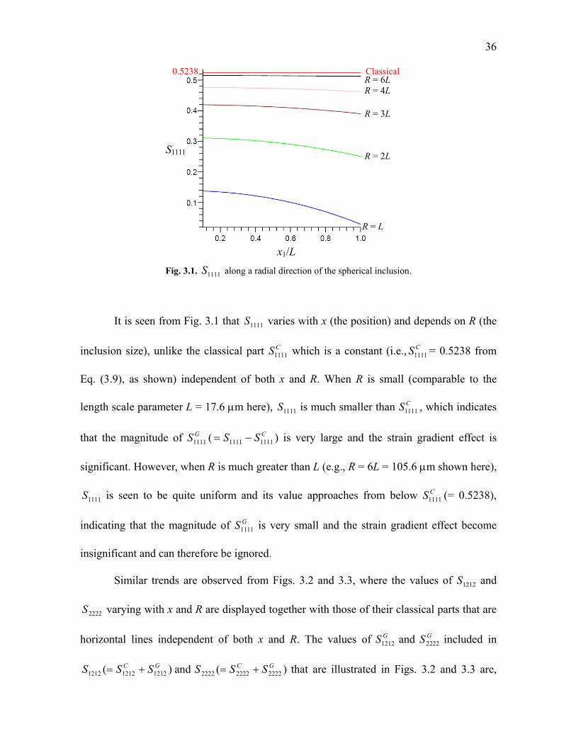
Fig. 3.1. 1111S along a radial direction of the spherical inclusion.

It is seen from Fig. 3.1 that 1111S varies with x (the position) and depends on R (the

inclusion size), unlike the classical part CS1111 which is a constant (i.e., CS1111 = 0.5238 from

Eq. (3.9), as shown) independent of both x and R. When R is small (comparable to the

length scale parameter L = 17.6 m here), 1111S is much smaller than CS1111 , which indicates

that the magnitude of GS1111 ( CSS 11111111 ) is very large and the strain gradient effect is

significant. However, when R is much greater than L (e.g., R = 6L = 105.6 m shown here),

1111S is seen to be quite uniform and its value approaches from below CS1111 (= 0.5238),

indicating that the magnitude of GS1111 is very small and the strain gradient effect become

insignificant and can therefore be ignored.

Similar trends are observed from Figs. 3.2 and 3.3, where the values of 1212S and

2222S varying with x and R are displayed together with those of their classical parts that are

horizontal lines independent of both x and R. The values of GS1212 and

GS2222 included in

)( 121212121212GC SSS and )( 222222222222

GC SSS that are illustrated in Figs. 3.2 and 3.3 are,

x1/L

S1111

Classical R = 6L

R = L

R = 2L

R = 3L

R = 4L

0.5238

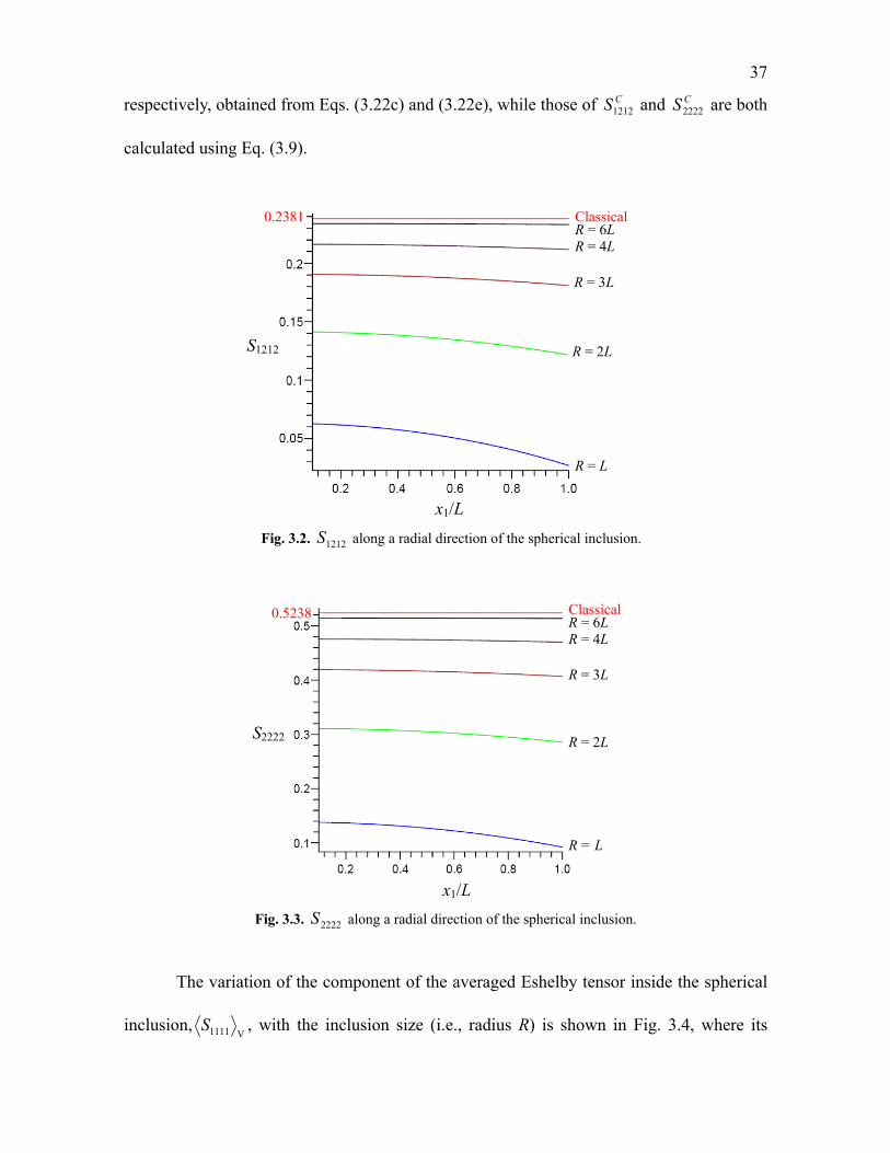
37

respectively, obtained from Eqs. (3.22c) and (3.22e), while those of CS1212 and CS2222 are both

calculated using Eq. (3.9).

Fig. 3.2. 1212S along a radial direction of the spherical inclusion.

Fig. 3.3. 2222S along a radial direction of the spherical inclusion.

The variation of the component of the averaged Eshelby tensor inside the spherical

inclusion,V1111S , with the inclusion size (i.e., radius R) is shown in Fig. 3.4, where its

x1/L

S2222

Classical R = 6L

R = L

R = 2L

R = 3L

R = 4L

0.5238

x1/L

S1212 R = 2L

R = 3L

0.2381

R = L

R = 4L R = 6L Classical

38

counterpart in classical elasticity, V1111

CS , is also displayed for comparison. Note that

V1111S is obtained from Eq. (3.18), while V1111

CS (= CS1111 = 0.5238) is from Eq. (3.9). The

material properties used here are v = 0.3 and L = 17.6 m, which are the same as those used

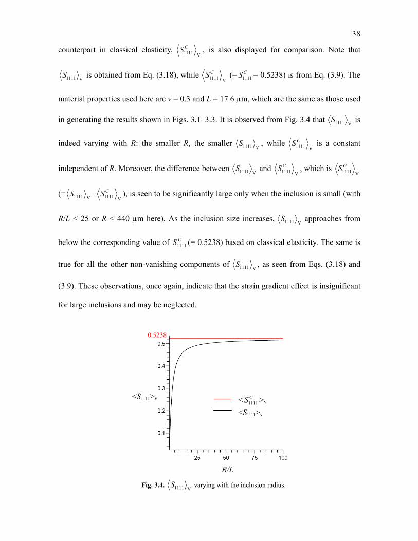
in generating the results shown in Figs. 3.1–3.3. It is observed from Fig. 3.4 that V1111S is

indeed varying with R: the smaller R, the smaller V1111S , while

V1111CS is a constant

independent of R. Moreover, the difference between V1111S and

V1111CS , which is

V1111GS

(=V1111S

V1111CS ), is seen to be significantly large only when the inclusion is small (with

R/L < 25 or R < 440 m here). As the inclusion size increases, V1111S approaches from

below the corresponding value of CS1111 (= 0.5238) based on classical elasticity. The same is

true for all the other non-vanishing components of V1111S , as seen from Eqs. (3.18) and

(3.9). These observations, once again, indicate that the strain gradient effect is insignificant

for large inclusions and may be neglected.

Fig. 3.4.

V1111S varying with the inclusion radius.

R/L

<S1111>v < CS1111 >v

<S1111>v

0.5238

39

Clearly, the numerical results presented above quantitatively show that the newly

obtained Eshelby tensor captures the size effect at the micron scale, unlike that based on

classical elasticity.

3.4. Summary

The Eshelby tensor for the spherical inclusion problem is explicitly obtained by

employing the general form of the non-classical Eshelby tensor derived in Chapter II using

the SSGET. To further illustrate this Eshelby tensor, sample numerical results are provided,

which reveal that the components of the new Eshelby tensor vary with both the position and

the inclusion size, thereby capturing the size effect at the micron scale.

In addition, the volume average of this new Eshelby tensor over the spherical

inclusion is derived in a closed form, which is needed in homogenization analyses. The

components of the averaged Eshelby tensor are found to decrease as the inclusion radius

decreases, and these components are observed to approach from below the values of the

corresponding components of the Eshelby tensor based on classical elasticity when the

inclusion size is large enough.

40

CHAPTER IV

ESHELBY TENSOR FOR A PLANE STRAIN

CYLINDRICAL INCLUSION

4.1. Introduction

The current chapter aims to apply the general formulas for a 3-D inclusion of

arbitrary shape obtained in Chapter II to solve the Eshelby cylindrical inclusion problem,

which is closely related to the fiber-reinforced composites (e.g., Luo and Weng, 1989) and

hence of great importance. The solution is derived in a closed form, and the Eshelby tensors

for the two regions inside and outside the cylindrical inclusion are obtained in explicit

expressions for the first time using a higher-order elasticity theory.

The rest of this chapter is organized as follows. In Section 4.2, the closed-form

expressions of the Eshelby tensor and the Eshelby-like tensor for a plane strain cylindrical

inclusion embedded in an infinite homogeneous isotropic elastic material are presented,

which have 15 and 30 independent components, respectively. The non-classical Eshelby

tensor is derived for the two regions inside and outside the inclusion, and the volume

average of the new Eshelby tensor over the cylindrical inclusion is exactly determined.

Numerical results are provided in Section 4.3 to quantitatively illustrate the position

dependence and the inclusion size dependence of the newly obtained Eshelby tensor for the

cylindrical inclusion. The chapter concludes in Section 4.4.

4.2. Eshelby Tensor for a Cylindrical Inclusion

A closed-form expression of the Eshelby tensor for a plane strain cylindrical

41

inclusion of infinite length embedded in an infinite homogeneous isotropic elastic body is

derived here by using the general formulas obtained in Chapter II.

Consider an infinitely long cylindrical inclusion of radius a whose symmetry axis

(central line) passes through the origin of the cylindrical coordinate system (r, x3) in the

physical space. In this case, (x), (x) defined in Eqs. (2.43a,b) can be obtained from their

derivatives given in Mura (1987) for both interior points (i.e., Ωx or x < a) and exterior

points (i.e., Ωx or x > a) as

Ω,,ln2

Ω,,)(Λ

22

12

x

x

CxR

Cxx

(4.1a,b)

Ω,,lnln2

1

Ω,,8

1

)(Φ

42224

324

x

x

CNxxxRxR

CMxxx

(4.2a,b)

where 2

2

2

1xxx x (unlike in the arbitrary 3-D case), and C1~C4 , M and N are

constants whose values are of no interest here since only the second-order derivatives of

and fourth-order derivatives of are involved in the expressions of S and T given in Eqs.

(2.44a–c) and (2.45), respectively. Also, (x) defined in Eq. (2.43c) can be evaluated to

obtain the following closed-form expressions (see Appendix D):

Ω,,4

,Ω,4)(Γ

01

10

x

x

L

xK

L

aLaI

L

aK

L

xaILL

x

(4.3a,b)

where In() and Kn() (n = 0, 1) are, respectively, the modified Bessel functions of the first

and second kinds of the nth order, which satisfy the following asymptotic relations (e.g.,

Arfken and Weber, 2005):

42

.2

~,2

1~ zase

zzKe

zzI Z

n

Z

n

(4.4)

Note that , and in Eqs. (4.1a,b)–(4.3a,b) are independent on the direction of the

position vector x due to the circular symmetry of the inclusion. Clearly, (x), (x) and (x)

are infinitely differentiable at any x 0.

Note that for this case, the inclusion is infinitely long and can be treated as in a

plane strain state, 2/12

2

2

1xxx x and the derivatives of (x), (x) and (x), defined

in Eq. (2.43a–c), with respect to x3 should vanish. Accordingly, the fourth-order Eshelby

tensor, S, and the fifth-order Eshelby-like tensor, T, will have expressions different from

those for the spherical inclusion, listed in Eqs. (3.4), (3.6) and (3.8), as will be seen below.

Using the expression of (x), (x) and (x), given in Eqs. (4.1)–(4.3) into the

general forms of S and T, given in Eqs. (2.44a–c) and (2.45), obtains the special

expressions of S and T for the plane strain cylindrical inclusion. Considering that the

general forms of S and T are expressed in terms of the derivatives of (x), (x) and (x)

with respect to xi, it is convenient to first give the following differential equations for a

sufficiently smooth function F(x) (with 2/122

21 xxx ).

,68

,

,

,46

,

,,

3343

25

2,

3154105,

23364,

232

42

,

233,

12,1,

FDxFDxxxxxFDxxxxF

FDxFDxxxFDxxxxxF

FDFDxxFDxxxxF

FDFDxxxFDxxxF

FDxFDxxxF

FDFDxxFFDxF

(4.5)

where use has been made of the results 2 and

43

.)()(

)()()(

,

,,

,

,10510545101

,151561

,331

,1

,

15

10

33

6

432

)4()5(

55

32

)4(

44

233221

xx

xxxx

xxxxxxxxxxxxxxx

xxxxxxxxxxxxxxxxxx

xxxx

xxxxxxxxxxxxxx

x

F

x

F

x

F

x

FF

xFD

x

F

x

F

x

FF

xFD

x

F

x

FF

xFD

x

FF

xFD

x

FFD

(4.6)

In Eq. (4.6), F = dF/dx, F = d2F/dx2, F = d3F/dx3, F(4) = d4F/dx4, and F(5) = d5F/dx5. Also,

in Eqs. (4.5) and (4.6) F can be replaced by (x), (x) or (x) involved in the general form

of the Eshelby tensor in Eqs. (2.44b,c) and the general form of the Eshelby-like tensor in

Eq.(2.45). Note that each Greek index ranges from 1 to 2 in Eqs. (4.5) and (4.6) and

throughout this dissertation unless otherwise stated.

After using Eqs. (4.5) and (4.6) in Eqs. (2.44b,c), the components of the Eshelby

tensor, with each index ranging from 1 to 2, for a plane strain cylindrical inclusion can be

obtained in the form of

),)(())((

)()()()()(0000

6

00000000

5

00

4

00

321

xxxxxJxxxxxxxxxJ

xxxJxxxJxJxJS

(4.7)

where xxx /0 is the component of the unit vector x/0 xx , and )(~)(

61xJxJ are

scalar-valued functions in terms of (x), (x), (x) and , which are different for each case

and will be individually given below. The superscript “” in Eq. (4.7) can be replaced by

“C” or “G” to represent the classical or the gradient part of the Eshelby tensor, respectively.

44

Clearly, S has 9 independent components (rather than 24 = 16 ones) due to the minor

symmetry (i.e., SSS ) exhibited by the Eshelby tensor.

For the classical part of the Eshelby tensor (i.e., CS), )(~)(

61xJxJ CC are obtained

as

,Φ)21(ΦΛ)1(4)21)(1(8

123

2

11DDxDv

vvJ C

,ΦΛ)1(2)1(8

1212

DDvv

J C

,Φ)41(ΦΛ)1(4)21)(1(8 34

2

2

2

3DvDxDvv

vv

xJ C

(4.8a–f)

Φ,)1(8 3

2

4D

v

xJ C

,ΦΛ)1()1(8 32

2

5DDv

v

xJ C

Φ.)1(8 4

4

6D

v

xJ C

Using Eqs. (4.8a–f) in Eq. (4.7) will yield the expression of CS

, which has 9 independent

components.

From Eqs. (2.44b) and (4.5), the other non-vanishing components of SC for a plane

strain cylindrical inclusion can be readily obtained as

ΛΛ8

112

200

33DDxxxS C

, (4.9a)

,Φ4Φ6Φ

ΛΛ)1(4)21)(1(8

23

002

4

400

12

200

33

DDxxxDxxx

DDxxxvvv

vS C

(4.9b)

where use has been made of the fact that the derivatives of x and x with respect to x3

involved in Eq. (2.44b) vanish. It is clear that CS33

has 3 independent components and

CS33

has 3 independent components.

45

For the gradient part of the Eshelby tensor (i.e., GS

), )(~)(61

xJxJ GG are found to

be

,)Λ(Γ)21()Λ(ΓΓ)1(2)21)(1(4

12

2

3

22

11

DLvDxvLDvv

vvJ G

,)Λ(ΓΓ)1()1(4

12

2

12

DLDv

vJ G

,)Λ(Γ)41()Λ(ΓΓ)1(2)21)(1(4 3

2

4

22

2

2

3

DLvDxvLDvv

vv

xJ G

),Λ(Γ)1(4 3

22

4

D

v

xLJ G

(4.10a–f)

,)Λ(Γ2Γ)1()1(8 3

2

2

2

5

DLDv

v

xJ G

).Λ(Γ)1(4 4

42

6

D

v

xLJ G

Substituting Eqs. (4.10a–f) into Eq. (4.7) will give the expression for GS , which

has 9 independent components. The other non-vanishing components of SG are obtained

from Eqs. (2.24c) and (4.5) as

12200

33 8

1DDxxxS G

, (4.11a)

,)ΛΓ(6)ΛΓ(Γ)1(2

)ΛΓ(4)ΛΓ(Γ)1(2)21)(1(4

3

2

4

22

2

200

2

2

3

22

133

DLDxLDvxxx

DLDxLDvvv

vS G

(4.11b)

where use has been made of the fact that the derivatives of (x), (x) and (x) with respect

to x3 involved in Eq. (2.44c) vanish. Clearly, GS33

has 3 independent components, and GS33

has 3 independent components.

By using Eq. (4.5) in Eq. (2.45), the components of the fifth-order Eshelby-like

tensor T, with each index ranging from 1 to 2, for a plane strain cylindrical inclusion can be

determined as

46

,GGG

G6G)8(G21

P)1(

P))(1(

PP21

)1(4

)1(8

315

0

4

3

10

000

5

500000

33

0

4

3000

3

0

5

5000

23

0

3

0

3

0

3

0

3

3000000000000

23

0

3

3000

2

xDxDxxxxDxxxxxx

xDxDxxxxxDxxxxv

v

xDxxxxv

Dxxxxxxxxxxxxxv

xDxDxxxxv

vv

v

LT

(4.12)

which includes 18 independent components. The other non-vanishing components of T are

obtained from Eqs. (2.45) and (4.5) as

PP8 23

0

3

0003

2

33DxxDxxxx

LT

, (4.13a)

which includes 6 independent components, and

,G6G8G

PP)1(4)21)(1(8

33

0

4

000

3

03

5

0005

23

0

3

0003

2

33

DxxDxxxxxDxxxx

DxxDxxxxvvv

vLT

(4.13b)

which contains 6 independent components. The functions P(x) and G(x) involved in Eqs.

(4.12) and (4.13a,b) are defined in terms of (x), (x) and (x) as

Γ)(Λ2Φ)G(Γ,Λ)P( 2 Lxx . (4.14)

Eqs. (4.7)–(4.13a,b) give the expressions for the components of the fourth-order

Eshelby tensor, S, and the fifth-order Eshelby-like tensor, T, based on the simplified strain

gradient theory for a plane strain cylindrical inclusion and with an infinite length in the x3

direction. As indicated earlier, for this plane strain inclusion problem, S has 15 independent

components and T has 30 independent components, which are in contrast to 36 and 108, the

numbers of independent components of S and T, respectively, in the general case of a 3-D

inclusion of arbitrary shape (see Eqs. (2.47a,b) and (2.48)). In addition, these expressions

for the components of S and T are in terms of the three scalar-valued functions (x), (x)

and (x), which are independent of x3 (with 2/12

2

2

1xxx x ).

47

Using Eqs. (4.1a) and (4.2a) along with Eqs. (4.6) and (4.8a–f) in the expression of

SC given in Eqs. (4.7) and (4.9a,b) leads to the non-zero components of the classical part of

the Eshelby tensor at any x inside the cylindrical inclusion (i.e., x or x < a) as

,)1(2

,4

1),(

)1(8

43

)1(8

143333

v

vSS

v

v

v

vS CCC

(4.15a–c)

which are identical to those based on classical elasticity (e.g., Mura, 1987). Note that Eqs.

(4.15a–c) list all 15 independent components of SC.

The use of Eqs. (4.1a), (4.2a) and (4.3a) in Eqs. (4.7), (4.10a–f) and (4.11a,b) gives

the expressions of the non-zero components of the gradient part of the Eshelby tensor SG

for points inside the inclusion (i.e., x or x < a) as

),)(())((

)()()()()(0000

6

00000000

5

00

4

00

321

xxxxxJxxxxxxxxxJ

xxxJxxxJxJxJSGG

GGGGG

(4.16)

where

,)2()1( 1

22

03

1

1ILvxLxI

xv

aKJ G

,)2()1( 1

222

03

1

2ILvxxLxI

xv

aKJ G

,)82()4()1( 1

222

0

22

3

1

3ILvxxLILvxx

Lxv

aKJ G

(4.17a–f)

,)8(4)1( 1

22

03

1

4ILxLxI

xv

aKJ G

,)82(2)8()1(2 1

222

0

222

3

1

5ILvxxLILvxxx

Lxv

aKJ G

,)6(8)24()1( 1

22

0

22

3

1

6ILxLILxx

Lxv

aKJ G

and

11000

133 )2(2

LILIxIxxKxL

aS G

, (4.18a)

)2(1 10

001

133 LIxIxxLI

xL

aK

v

vS G

. (4.18b)

48

In Eqs. (4.17a–f) and (4.18a,b), I0 = I0( Lx

), I1 = I1( Lx

) and K1 = K1( La

) are modified Bessel

functions of the indicated arguments, with x < a. Eqs. (4.16)–(4.18a,b) provide the explicit

expressions of all 15 independent components of SG.

It is clearly seen from Eqs. (4.15a–c) that the classical part of the Eshelby tensor, SC,

is independent of x, a and L and is therefore uniform inside the cylindrical inclusion. In

contrast, the gradient part, SG, given by Eqs. (4.16)–(4.18a,b) depends on x, a and L in a

complicated manner. That is, SG is non-uniform inside the cylindrical inclusion and differs

for materials with different values of a (the inclusion size) and/or L (the material length

scale parameter). However, if the strain gradient effect is not considered, then L = 0 (so that

x/L , a/L ) and Eqs. (4.4), (4.16)–(4.18a,b) give 0GijlmS . It thus follows from Eq.

(2.44a) that S = SC. That is, the Eshelby tensor for the cylindrical inclusion derived here

using the simplified strain gradient elasticity theory reduces to that based on classical

elasticity when L = 0.

Considering that SG is position-dependent inside the inclusion, the volume average

of SG over the cylindrical inclusion will be needed in calculating the volume average of S

(= SC + SG) to be used for predicting the effective properties of a heterogeneous fiber-

reinforced composite. Hence, the volume average of SG is evaluated next.

Note that the volume average of a sufficiently smooth function F(x) (with

2

2

2

1xxx x ) over the domain u occupied by the cylindrical inclusion of a unit

length is defined by

a

dxdxFa

FdVF0

2

02Ωu

V

1

)Ω(Vol

1u

, (4.19)

where use has been made of the volume element 3dxdxdxdV in the cylindrical

49

coordinate system (r, x3) (with r = 2/122

21 xxx ) and the fact that F = F(x) is

independent of x3. In Eq. (4.19) and throughout this chapter, the volume average over the

inclusion domain uis denoted by the symbolV

.

Consider the transformation from the Cartesian to the cylindrical coordinate system:

.sin,cos 02

01 xx (4.20)

It follows from Eq. (4.20) that

dxx 02

0

0 , )(4

0002

0

0

dxxxx . (4.21a,b)

Applying Eqs. (4.19) and (4.21a,b) to Eqs. (4.7), (4.10a–f) and (4.11a,b) leads to the

volume average of the gradient part of the Eshelby tensor, V

GS , as

)(

4

122

4

12

165264312V GGGGGGGG JJJJJJJ

aS , (4.22)

,Γ2Γ8 0 12

22V33

aG xdxDDxa

S

(4.23)

,)Λ(Γ)Λ(Γ8)Λ(Γ8

Γ2Γ)1(2)21)(1(4

44

32

22

0 122

2V33

xdxDxDxDL

DDxvavv

vS

aG

(4.24)

where

a G

n

G

ndxxJxJ 0 )( (n =1, 2, ..., 6), (4.25)

with G

nJ (n = 1, 2, ..., 6) to be substituted from Eqs. (4.10a–f). The six integrals for GG JJ

61~

defined in Eq. (4.25) can be exactly evaluated with the help of the following results:

111 )(1

cFDdxFDdx

d

xxdxFxD nnn (n = 1, 2, ..., 5),

,Γ2'Γ'Γ2)''Γ()'Γ''Γ(Γ 223 cxdxxdxxdxDx

,'Γ

3''Γ)'Γ

3''Γ

3'''Γ(Γ 3233 c

xdx

xxdxDx

50

,'Γ

15''Γ7'''Γ])''Γ

(15'''Γ7)''''Γ[(Γ 445 c

xxdx

xxdxDx (4.26)

where c1~c4 are integration constants, F is a smooth function of x (with 2

2

2

1xxx x )

which can be (x), (x) or (x), D1F~D5F are differentials defined in Eq. (4.6), and D0F

F.

It then follows from Eqs. (4.10a–f), (4.1a), (4.3a) and (4.22)–(4.26) that the volume

averages of the non-zero components of the gradient part of the Eshelby tensor,V

GS , are

L

aI

L

aK

v

v

v

vS G

11V)(

)1(4

34

)1(4

41 , (4.27a)

L

aI

L

aKS G

11V33 2

1, (4.27b)

L

aI

L

aK

v

vS G

11V33 1, (4.27c)

where I1() and K1() are modified Bessel functions of the indicated argument La . A

comparison of the expressions of V

GS in Eqs. (4.27a–c) with those of V

CS SC given in

Eqs. (4.15a–c) shows that

Cijkl

Gijkl S

L

aI

L

aKS

11V

2 . (4.28)

Hence, the volume average of the Eshelby tensor over the cylindrical inclusion of the unit

length is obtained from Eqs. (2.44a), (4.15a–c), (4.19) and (4.28) as

C

ijklijkl SL

aI

L

aKS

11V

21 , (4.29)

where CijklS are given in Eq. (4.15a–c). Eq. (4.29) shows that

VijklS depends on a/L.

When L = 0 (or a/L ), Eq. (4.4) gives

L

aI

L

aK 11 0, and hence Eq. (4.29) reduces

to C

ijklijkl SS V

, as will be further illustrated in the next section. Based on the closed-form

expression of the average Eshelby tensor derived in Eq. (4.29), the inhomogeneity problem

51

involving the cylindrical inclusion of a different material (e.g., Mura, 1987) and the related

homogenization of strain gradient composites reinforced by cylindrical fibers can then be

analyzed by using Eshelby’s equivalent eigenstrain method, as was done by Xun et al.

(2004) for micropolar composites.

The volume averages of the components of the fifth-order Eshelby-like tensor T

inside the cylindrical inclusion of the unit length are, based on Eq. (4.19),

a

ijklmijklm dxxdTa

T0

2

02V

1

(4.30)

where Tijklm, given in Eqs. (4.12) and (4.13a,b), is odd in 0x . As a result, the integration of

Tijklm with respect to on the interval of [0, 2] vanishes, thereby leading to VijklmT = 0.

Finally, the Eshelby tensor for exterior points x (or x > a) can be similarly

determined as follows. Using Eqs. (4.1b), (4.2b), (4.3b) and (4.6) in Eqs. (4.7)–(4.9a,b)

yields the non-vanishing components of SC as

,)23(8)

)((4)(4)2(4

))(24()24()1(8

000022000000

0022002200222

2222224

2

xxxxxRxxxxxx

xxRvxxxRxxxRxvx

RxvxRxvxxv

RS C

(4.31a)

002

2

33 24 xx

x

RS C , (4.31b)

002

2

33 2)1(2 xx

x

R

v

vS C

, (4.31c)

which are the same as those of the Eshelby tensor outside a cylindrical inclusion based on

classical elasticity (Cheng and He, 1997). Clearly, Eqs. (4.31a–c) show that the classical

part of the Eshelby tensor, SC, is not uniform outside the inclusion (with x or x > a) but

changes with x, which is the distance from x (the point of interest) to the central line of the

cylindrical inclusion. This is different from the case for x inside the inclusion (with Ωx .

52

or x < a), where SC is uniform for all Ωx , as shown in Eqs. (4.15a–c)..

Substituting Eqs. (4.1b), (4.2b), (4.3b) and (4.6) into Eqs. (4.10a–f) and (4.11a,b)

yields

,)1(

)2()1( 4

22

122

031

1 xv

RLKLvxLxK

xv

aIJ G

(4.32a)

,)1(

)2()1( 4

22

1222

031

2 xv

RLKLvxxLxK

xv

aIJ G

(4.32b)

,)1(

4)82()4(

)1( 4

22

1222

022

31

3 xv

RLKLvxxLKLvxx

Lxv

aIJ G

(4.32c)

,)1(

4)8(4

)1( 4

22

122

031

4 xv

RLKLxLxK

xv

aIJ G

(4.32d)

,)1(

4)82(2)8(

)1(2 4

22

1222

0222

31

5 xv

RLKLvxxLKLvxxx

Lxv

aIJ G

(4.32e)

,)1(

24)6(8)24(

)1( 4

22

122

022

31

6 xv

RLKLxLKLxx

Lxv

aIJ G

(4.32f)

and

11000

133 )2(2

LKLKxKxxIxL

aS G

, (4.33a)

)2(1 10

001

133 LKxKxxLK

xL

aI

v

vS G

. (4.33b)

In Eqs. (4.32a–f) and (4.33a,b), I1 = I1( La

), K0 = K0( Lx

) and K1 = K1( Lx

) are modified

Bessel functions of the indicated arguments, with x > a. Using Eqs. (4.32a–f) in Eq. (4.7)

will then yield the expression for GS , which has 9 independent components. The other 6

non-vanishing components of SG in this case are obtained from Eqs. (4.33a,b). It is

observed from Eqs. (4.7), (4.4), (4.32a–f) and (4.33a,b) that the components of SG in this

exterior case (with x or x > a) will vanish when L = 0 (or x/L , a/L ). By

substituting the components of SG obtained here and the components of SC derived in Eqs.

(4.31a–c) into Eq. (2.44a) will finally give the explicit expressions of the Eshelby tensor S

(= SC + SG) for any point x outside the cylindrical inclusion (i.e., x or x > a).

53

4.3. Numerical Results

In this section, some numerical results are presented to quantitatively illustrate how

the components of the Eshelby tensor for the cylindrical inclusion vary with position and

inclusion size, which has been analytically demonstrated in the preceding section.

From Eqs. (4.16)–(4.18a,b), the non-zero components of the gradient part of the

Eshelby tensor, SG, for any x inside the cylindrical inclusion (i.e., x or x < a) along the

x1 axis (with x2 = 0, x = x1) can be obtained as

,)6()3()1( 1

22

0

222

3

1

1111ILvxLIxvxLx

Lxv

aKS G

(4.34a)

,3)26()1( 01

222

3

1

2222LxIIxvxL

xv

aKS G

(4.34b)

,)6()3()1( 1

2220

223

11122 IxLvxLIvxLx

Lxv

aKS G

(4.34c)

1222

031

2211 )6(3)1(

IvxxLLxIxv

aKS G

, (4.34d)

122

0222

31

1212 )6(2)6()1(2

ILxLIvxxLxLxv

aKS G

, (4.34e)

1132321013131 2),(

2IK

x

aSLIxIK

xL

aS GG , (4.34f,g)

x

IaK

v

vSLIxI

xL

aK

v

vS GG 11

2233101

1133 1),(

1

, (4.34h,i)

where I0 = I0( Lx

), I1 = I1( Lx

) and K1 = K1( La

) are modified Bessel functions of the indicated

arguments. As shown in Eqs. (4.34a–i), in this special case (with x = x1, x2 = 0) there are

only 9 non-zero components among the 15 independent non-zero components of SG.

The distribution of GC SSS 111111111111 along the x1 axis (a generic radial direction of

the inclusion due to the axial symmetry) for five different values of a is shown in Fig. 4.1,

where the values of CS1111 and

GS1111 are, respectively, obtained from Eqs. (4.15a) and (4.34a).

For illustration purpose, in the numerical analysis leading to the results displayed in Figs.

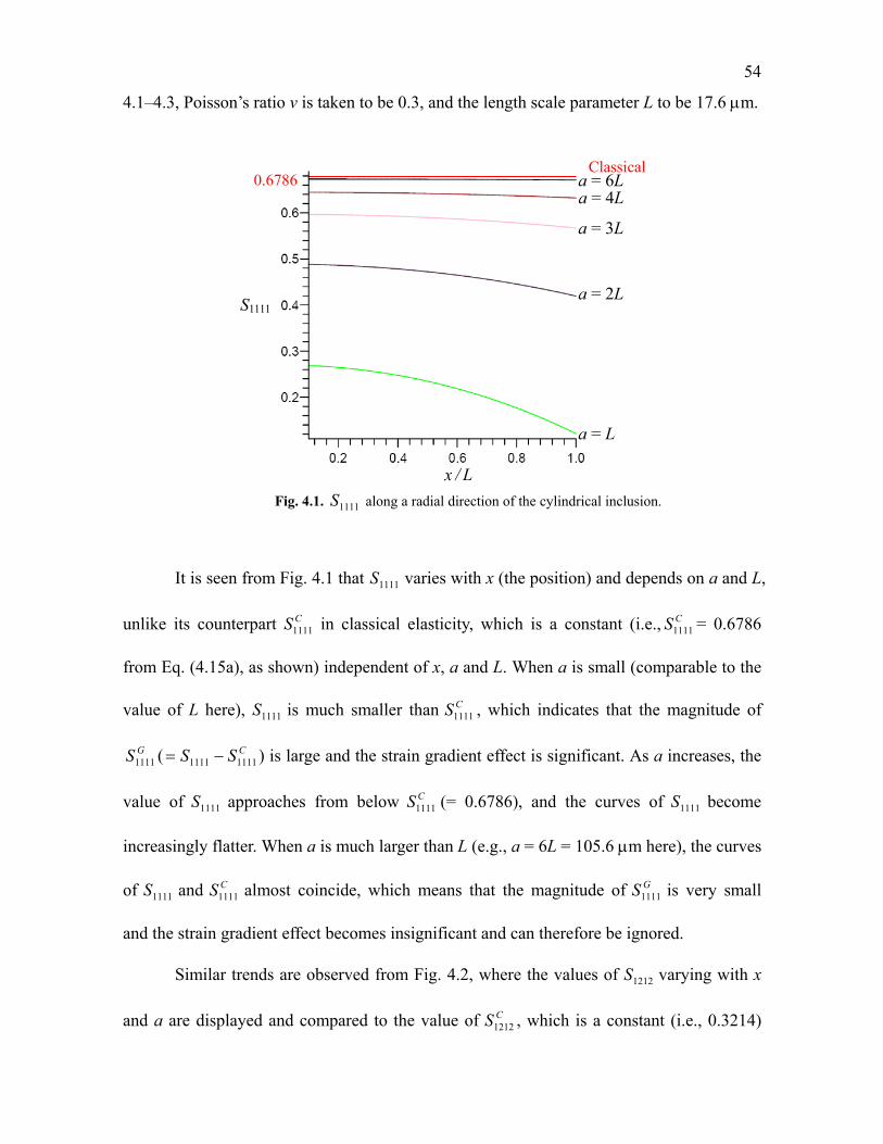
54

4.1–4.3, Poisson’s ratio v is taken to be 0.3, and the length scale parameter L to be 17.6 m.

Fig. 4.1. 1111S along a radial direction of the cylindrical inclusion.

It is seen from Fig. 4.1 that 1111S varies with x (the position) and depends on a and L,

unlike its counterpart CS1111 in classical elasticity, which is a constant (i.e., CS1111 = 0.6786

from Eq. (4.15a), as shown) independent of x, a and L. When a is small (comparable to the

value of L here), 1111S is much smaller than CS1111 , which indicates that the magnitude of

GS1111 ( CSS 11111111 ) is large and the strain gradient effect is significant. As a increases, the

value of 1111S approaches from below CS1111 (= 0.6786), and the curves of 1111S become

increasingly flatter. When a is much larger than L (e.g., a = 6L = 105.6 m here), the curves

of 1111S and CS1111 almost coincide, which means that the magnitude of

GS1111 is very small

and the strain gradient effect becomes insignificant and can therefore be ignored.

Similar trends are observed from Fig. 4.2, where the values of 1212S varying with x

and a are displayed and compared to the value of CS1212 , which is a constant (i.e., 0.3214)

a = L

a = 2L

a = 3L

a = 4L a = 6L

x / L

0.6786

S1111

Classical

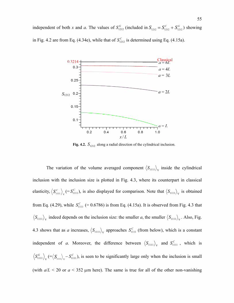
55

independent of both x and a. The values of GS1212 (included in

GC SSS 121212121212 ) showing

in Fig. 4.2 are from Eq. (4.34e), while that of CS1212 is determined using Eq. (4.15a).

Fig. 4.2. 1212S along a radial direction of the cylindrical inclusion.

The variation of the volume averaged component V1111S inside the cylindrical

inclusion with the inclusion size is plotted in Fig. 4.3, where its counterpart in classical

elasticity, V1111

CS (= CS1111), is also displayed for comparison. Note that V1111S is obtained

from Eq. (4.29), while CS1111 (= 0.6786) is from Eq. (4.15a). It is observed from Fig. 4.3 that

V1111S indeed depends on the inclusion size: the smaller a, the smaller V1111S . Also, Fig.

4.3 shows that as a increases, V1111S approaches CS1111 (from below), which is a constant

independent of a. Moreover, the difference between V1111S and CS1111 , which is

V1111GS (=

V1111S CS1111), is seen to be significantly large only when the inclusion is small

(with a/L < 20 or a < 352 m here). The same is true for all of the other non-vanishing

S1212

x / L

a = L

a = 2L

a = 3L a = 4L

a = 6L0.3214 Classical

56

components of VijklS , which is mathematically dictated by Eq. (4.29). These observations

indicate that the strain gradient effect is insignificant for large inclusions and may therefore

be neglected, which agrees with what is observed above from examining Figs. 4.1 and 4.2.

Fig. 4.3.

V1111S varying with the inclusion radius.

4.4. Summary

The Eshelby tensor for a cylindrical inclusion in the two regions inside and outside

the inclusion is obtained in explicit expressions for the first time using the general form of

the Eshelby tensor for a plane strain inclusion based on the strain gradient theory. The

newly obtained Eshelby tensor has 15 independent non-zero components (as opposed to 36

such components in the case of a 3-D inclusion of arbitrary shape) and consists of a

classical part (depending only on Poisson’s ratio) and a gradient part (depending on the

length scale parameter additionally). The gradient part vanishes when the strain gradient

effect is not considered. This non-classical Eshelby tensor contains a material length scale

parameter and can explain the size effect at the micron scale, unlike that based on classical

elasticity. When the strain gradient effect is suppressed, this Eshelby tensor reduces to that

a / L

<S1111> V1111CS

V1111S

0.6786

57

for a cylindrical inclusion based on classical elasticity.

To further illustrate the newly derived Eshelby tensor, sample numerical results are

provided. These results quantitatively show that the new Eshelby tensor depends on both

the position and inclusion size and can capture the size effect at the micron scale.

In addition, the volume average of the newly derived position-dependent Eshelby

tensor over the cylindrical inclusion of a unit length is obtained in a closed form, which is

needed in homogenization analyses of fiber-reinforced composites. The volume averaged

components of the Eshelby tensor are found to become smaller as the inclusion radius

decreases, but they are observed to approach (from below) the constant values of the

corresponding components of the Eshelby tensor based on classical elasticity when the

inclusion size becomes sufficiently large.

58

CHAPTER V

STRAIN GRADIENT SOLUTION FOR

ESHELBY’S ELLIPSOIDAL INCLUSION

PROBLEM

5.1. Introduction

The simplified strain elasticity theory (SSGET) introduced in Chapter II has been

found a success in capturing the size effect exhibited by composite materials filled with

inhomogeneities of micron scale, as discussed in the preceding chapters. A spherical

inclusion and a cylindrical inclusion problem have been solved in the framework of the

SSGET. This chapter aims to solve a more general and complex ellipsoidal inclusion

problem based on the SSGET, which are of fundamental interest in a wide range of physical

and engineering problems in the micromechanics of heterogeneous solids.

The rest of this chapter is organized as follows. In Section 5.2, analytical

expressions of the Eshelby tensor inside and outside an ellipsoidal inclusion are deduced by

applying the general form of the Eshelby tensor derived in Chapter II. The volume average

of this Eshelby tensor over the ellipsoidal inclusion is analytically evaluated. Numerical

results are provided in Section 5.3 to quantitatively illustrate the position dependence and

the inclusion size dependence of the newly obtained Eshelby tensor for the ellipsoidal

inclusion problem. This chapter concludes with a summary in Section 5.4.

5.2. Ellipsoidal Inclusion

Consider an ellipsoidal inclusion of three semi-axes a1, a2 and a3 and centered at the

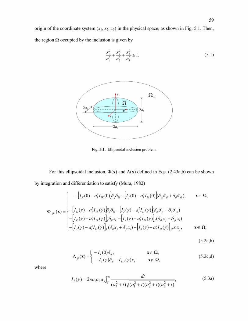
59

origin of the coordinate system (x1, x2, x3) in the physical space, as shown in Fig. 5.1. Then,

the region occupied by the inclusion is given by

.123

23

22

22

21

21

a

x

a

x

a

x (5.1)

12a

22a

32a

3e

1e

2e

Fig. 5.1. Ellipsoidal inclusion problem.

For this ellipsoidal inclusion, (x) and (x) defined in Eqs. (2.43a,b) can be shown

by integration and differentiation to satisfy (Mura, 1982)

Ω;,)()()()()(

)()()()()(

)()()()()(

Ω,),()0()0()0()0(

)(Φ

,2

,2

,2

,2

22

22

,

x

x

x

jiklIJIJijljilkIJIJ

ijkjiklIJIJkijlIKIK

jkiljlikIJIJklijIKIK

jkiljlikIJIJklijIKIK

ijkl

xxIaIxxIaI

xxIaIxIaI

IaIIaI

IaIIaI

(5.2a,b)

Ω,,)()(

Ω,,)0()(Λ

,, x

xx

ijIijI

ijIij xII

I

(5.2c,d)

where

,))()(()(

2)(23

22

21

2321

tatatata

dtaaaπI

I

I (5.3a)

60

,))()(())((

2)(23

22

21

22321

tatatatata

dtaaaπI

JI

IJ (5.3b)

which are functions of , with I, J1, 2, 3. For x (interior points) = 0, and for x

(exterior points) is the largest positive root of the following equation:

123

23

22

22

21

21

a

x

a

x

a

x , (5.4)

which shows that is a function of x. Note that in Eqs. (5.2a–d) and in the sequel each

repeated lower-case index implies summation from 1 to 3, while each upper-case index

takes the same value as its corresponding lower-case index but implies no summation.

For interior points with x , it follows from Eqs. (2.47a) and (5.2a,c) that the

classical part of the Eshelby tensor is

,)()0()0()0()1()0()1(

)0()0()0(2)1(8

1

2

2,

jlimjmilIJIJML

lmijILILIINC

ijlm

δδδδIaIIvIv

δδIaIvIvπ

S

(5.5)

which is the same as that provided in Li and Wang (2008). It is clear from Eq. (5.5) that the

Eshelby tensor INCijlmS , is uniform (i.e., independent of position x) inside the ellipsoidal

inclusion, which is a well-known result (e.g., Markenscoff, 1998) and has recently been

elaborated in a broader context by Liu (2008). In fact, it can be shown that the components

of INCijlmS , given in Eq. (5.5) depend only on the two aspect ratios of the ellipsoidal inclusion,

defined by α1 = a1/a3 and α2 = a2/a3, and Poisson’s ratio of the matrix material, .

For exterior points with x , it can be shown that the use of Eqs. (2.47a) and

(5.2b,d) yields the classical part of the Eshelby tensor as (Mura, 1982)

61

,)()()()()(

)()()()()()1(8

1)(

)()()(8

1)(

)1(4)(

,2

,2

,2

,2

,

,,,,,

jilmIJIJijmjimlIJIJ

ijljilmIJIJlijmILILmjliM

miljMljmiLlimjLilmjICijlm

EXCijlm

xxIaIxδxδIaI

xδxδIaIxδIaIvπ

xδI

xδIxδIxδIπ

xδIvπ

vSS

(5.6)

where

.)()()()()1()()1(

)()()(2)1(8

1)(

2

2

jlimjmilIJIJML

lmijILILICijlm

δδδδIaIIvIv

δδIaIvIvπ

S

(5.7)

Clearly, Eq. (5.6) involves the first- and second-order derivatives of II() and IIJ() defined

in Eqs. (5.3a,b), which are not explicit and will be replaced with more direct expressions. It

can be shown from Eqs. (5.3a,b), after some lengthy algebra, that

,4

)(,4

)( 321,

321,

pPJI

pIJpPJ

pJ

xaaaI

xaaaI

(5.8a,b)

,ˆˆˆˆˆˆ4

224

)()( 321,

2

jipqPqpjiQPJIpqIJIJji nnnnnn

Z

aaaIaIxx

(5.8c) where

,)(

,))()((22

23

22

21

M

mm

a

xxZaaa

2

1

II a

, (5.9a–c)

1 2 3 2 3 2ˆ, , .

( ) ( )m m i

iM I

x x xn

a a Z

(5.9d–f)

Using Eqs. (5.7) and (5.8a–c) in Eq. (5.6) then gives

,

)()(

)(

)7(

)6()5(

)4()3()2()1(,

mljiIJLM

lijmLImijlMIJljimLJmjilMJI

jilmJILmlijMLIjlimjmilIJlmijILEXC

ijlm

xxxxS

xxxxSxxxxS

xxSxxSSSS

(5.10)

where

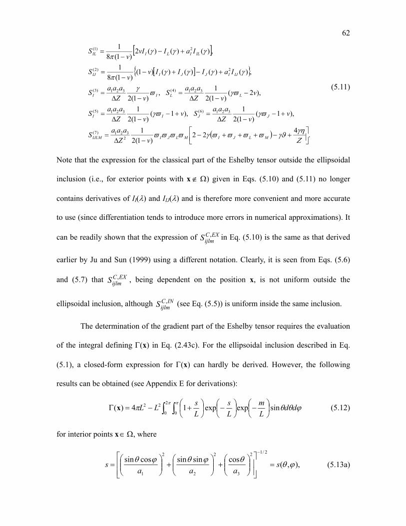
62

.4

22)1(2

1

),1()1(2

1),1(

)1(2

1

),2()1(2

1,

)1(2

,)()()()()1()1(8

1

,)()()(2)1(8

1

2321)7(

321)6(321)5(

321)4(321)3(

2)2(

2)1(

MLJIMLJIIJLM

JJII

LLII

IJIJJIIJ

ILILIIL

vZ

aaaS

vvZ

aaaSv

vZ

aaaS

vvZ

aaaS

vZ

aaaS

IaIIIvv

S

IaIvIv

S

(5.11)

Note that the expression for the classical part of the Eshelby tensor outside the ellipsoidal

inclusion (i.e., for exterior points with x ) given in Eqs. (5.10) and (5.11) no longer

contains derivatives of II() and IIJ() and is therefore more convenient and more accurate

to use (since differentiation tends to introduce more errors in numerical approximations). It

can be readily shown that the expression of EXCijlmS , in Eq. (5.10) is the same as that derived

earlier by Ju and Sun (1999) using a different notation. Clearly, it is seen from Eqs. (5.6)

and (5.7) that EXCijlmS , , being dependent on the position x, is not uniform outside the

ellipsoidal inclusion, although INCijlmS , (see Eq. (5.5)) is uniform inside the same inclusion.

The determination of the gradient part of the Eshelby tensor requires the evaluation

of the integral defining (x) in Eq. (2.43c). For the ellipsoidal inclusion described in Eq.

(5.1), a closed-form expression for (x) can hardly be derived. However, the following

results can be obtained (see Appendix E for derivations):

2

0 0

22 sinexpexp14)( ddL

m

L

s

L

sLLx (5.12)

for interior points x , where

),,(cossinsincossin

2/12

3

2

2

2

1

s

aaas

(5.13a)

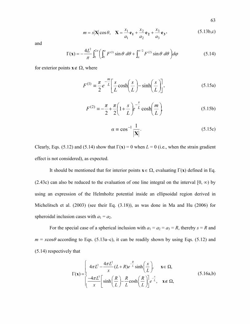
63

321 eeeXX3

3

2

2

1

1,cosa

x

a

x

a

xθsm , (5.13b,c)

and

ddFdF

L

2

0

2/ )2(

0

)1(2

sinsin4

)(Γ x (5.14)

for exterior points x , where

L

s

L

s

L

se

πF L

m

sinhcosh2

)1( , (5.15a)

,cosh122

)2(

L

me

L

sππF L

s

(5.15b)

X

1cos 1α . (5.15c)

Clearly, Eqs. (5.12) and (5.14) show that (x) = 0 when L = 0 (i.e., when the strain gradient

effect is not considered), as expected.

It should be mentioned that for interior points x , evaluating (x) defined in Eq.

(2.43c) can also be reduced to the evaluation of one line integral on the interval [0, ) by

using an expression of the Helmholtz potential inside an ellipsoidal region derived in

Michelitsch et al. (2003) (see their Eq. (3.18)), as was done in Ma and Hu (2006) for

spheroidal inclusion cases with a1 = a2.

For the special case of a spherical inclusion with a1 = a2 = a3 = R, thereby s = R and

m = xcos according to Eqs. (5.13a–c), it can be readily shown by using Eqs. (5.12) and

(5.14) respectively that

22

3

44 ( ) sinh , Ω,

Γ( )4

sinh cosh , Ω,

R

L

x

L

L xL L R e

x L

L R R Re

x L L L

x

x

x

(5.16a,b)

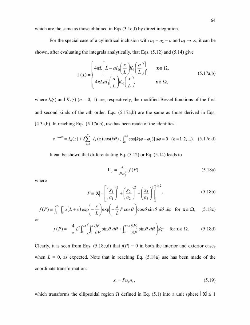
64

which are the same as those obtained in Eqs.(3.1e,f) by direct integration.

For the special case of a cylindrical inclusion with a1 = a2 = a and a3 , it can be

shown, after evaluating the integrals analytically, that Eqs. (5.12) and (5.14) give

Ω,,4

,Ω,4)(Γ

01

10

x

xx

L

xK

L

aLaIπ

L

aK

L

xaILLπ

(5.17a,b)

where In() and Kn() (n = 0, 1) are, respectively, the modified Bessel functions of the first

and second kinds of the nth order. Eqs. (5.17a,b) are the same as those derived in Eqs.

(4.3a,b). In reaching Eqs. (5.17a,b), use has been made of the identities:

)cos()(2)(1

0cos kzIzIe k

k

z

, ...).,2,1(0)](cos[2

0 0 kdk

(5.17c,d)

It can be shown that differentiating Eq. (5.12) or Eq. (5.14) leads to

),(Γ2, Pf

Pa

x

I

ii (5.18a)

where 2/12

3

32

2

22

1

1

a

x

a

x

a

xP X , (5.18b)

2

0 0sincoscosexpexp)( ddP

L

s

L

ssLsPf for x , (5.18c)

or

dd

P

Fd

P

FLPf

2

0

2/2

0

12 sinsin4

)( for x . (5.18d)

Clearly, it is seen from Eqs. (5.18c,d) that f(P) = 0 in both the interior and exterior cases

when L = 0, as expected. Note that in reaching Eq. (5.18a) use has been made of the

coordinate transformation:

iIi nPax , (5.19)

which transforms the ellipsoidal region defined in Eq. (5.1) into a unit sphere X 1

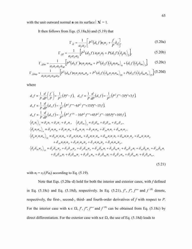
65

with the unit outward normal n on its surface X= 1.

It then follows from Eqs. (5.18a,b) and (5.19) that

,1

Γ 12

,

ijji

JIij δ

Pf

nnfdPaa

(5.20a)

,)()(1

Γ312

3, lijlji

LJIijl nδfdPnnnfdP

aaa (5.20b)

,1Γ

31622

34

, lmijmlijmljiMLJI

ijlm δδfdnnδfdPnnnnfdPaaaa

(5.20c)

,)()()(1

Γ152103

34

5, plmijmljippmlji

PMLJIijlmp nδδfdPnnnδfdPnnnnnfdP

aaaaa (5.20d)

where

,

,

,

,,

,105'105''45'''1011

,15'15''6'''11

,3'3''11

,'11

15

10

6

33

23)4(4

934

23

723

251231

mlpijlmpijmjlipimpjlmjpiljmpilljmip

ilpjmjlpimljpimjlmipilmjppimjlpjmilplmijplmij

pmlijpmijlpmjilplijm

pljimpjilmljimpmjilpmlijpmljipmljip

jilmlijmmijlljimmjilmlijmlij

jlimjmillmijlmijijljillijlij

nnnnnnn

nnnnnnnnn

nnnnnnnnnnnn

nnnnnnnnnnnnnnnnnnnnn

nnnnnnnnnnnnnn

nnnn

fPffPfPfPP

fddP

d

Pfd

fPffPfPP

fddP

d

Pfd

fPffPP

fddP

d

PfdfPf

PP

f

dP

d

Pfd

(5.21)

with ni = xi/(PaI) according to Eq. (5.19).

Note that Eqs. (5.20a–d) hold for both the interior and exterior cases, with f defined

in Eq. (5.18c) and Eq. (5.18d), respectively. In Eq. (5.21), f , f, f and f (4) denote,

respectively, the first-, second-, third- and fourth-order derivatives of f with respect to P.

For the interior case with x , f , f, f and f (4) can be obtained from Eq. (5.18c) by

direct differentiation. For the exterior case with x , the use of Eq. (5.18d) leads to

66

,sinsin4

,sinsin4

,sinsin4

,sinsin4

2

0

2/

5

)2(5

0 5

)1(52)4(

2

0

2/

4

)2(4

0 4

)1(42

2

0

2/

3

)2(3

0 3

)1(32

2

0

2/

2

)2(2

0 2

)1(22

ddP

Fd

P

FLf

ddP

Fd

P

FLf

ddP

Fd

P

FLf

ddP

Fd

P

FLf

(5.22)

where F(1) and F(2) are defined in Eqs. (5.15a,b). In reaching Eq. (5.22) use has also been

made of the result [F(1)F(2)] = = 0, which enables the terms involving /P to vanish.

Using Eqs. (5.20a,c) in Eq. (2.47b) then yields the gradient part of the Eshelby

tensor as

,22

)1(

)1(2

)1(8

1

,2

31622

34

2

12

12

ijlmlmijmlijmljiMLJI

LJ

jlim

MI

jlim

MJ

jmil

LI

jmil

LI

lijm

LJ

ljim

MI

mijl

MJ

mjillmijji

JI

Gijlm

LδδfdnnδfdPnnnnfdPaaaa

L

aa

δδ

aa

δδ

aa

δδ

aa

δδ

P

fv

aa

nnδ

aa

nnδ

aa

nnδ

aa

nnδfdPvδδ

P

fnnfdP

aa

v

vπS

(5.23)

where ni = xi/(PaI) from Eq (5.19), and P is defined in Eq. (5.18b).

Equation (5.23) applies to both the interior and exterior cases, but the expressions

for f(P) and ,ijlm are different in each case. For the interior case with x , f(P) is given in

Eq. (5.18c) and ,ijlm = 0 (see Eq. (5.2c)), while for the exterior case with x , f(P) is

provided in Eq. (5.18d) and ,ijlm is obtained from Eq. (5.2d), after some lengthy algebra, as

,)

(2

4)(1

4 321,

IJLjilmIJLlijm

IJMmijlIJLljimIJMmjilILMmlij

IJLMmljiJIjlimJIjmilLIlmijijlm

MxxMxx

MxxMxxMxxMxx

ΝxxxxZ

aaa

( 5.24)

where

67

ZZM MLIMLIILM

2

2

1)(

12 , (5.25a)

,12)2(3

2

1

4

1))(

6(

)()(1

2

22

222223

ZZZ

ZΝ

MLJI

MLJIMLJIMLJIIJLM

(5.25b)

,23

22

21 2

343

22

42

21

41 xxx . (5.25c,d)

From Eqs. (5.23)–(5.25a–d) it is seen that the gradient part of the Eshelby tensor,

GijlmS , is position-dependent inside and outside the ellipsoidal inclusion, since f, P, ni, and

,ijlm (for the exterior case) involved in GijlmS are all functions of x. This differs from the

classical part, INCijlmS , , which is uniform inside the same inclusion.

Next, substituting Eqs. (5.20b,d) into Eq. (2.48) gives the fifth-order Eshelby-like

tensor as

],)2()Λ)(1(2

)1(8

)()()(2

))(()1(

))(()1(

)()(21

)1(8

,2

,,,,,

2

1521033

452

33331

23

3123

2

ijlmpimjlpjmilpiljmpjlimplmijp

plmijmljippmlji

MIimpjlMJjmpilLIilpjmLJjlmip

MIimpljMJjmpliLIilpmjLJjlpmi

jippjiMLlmPMLJI

ijlmp

Lδδδδvδvvπ

L

nδδfdPnnnδfdPnnnnnfdPL

aaδnδaaδnδaaδnδaaδnδfdPv

aaδnnnaaδnnnaaδnnnaaδnnnfdPv

nδfdPnnnfdPaaδvaaaaavπ

LT

(5.26)

where ni = xi/(PaI) from Eq (5.19), P is defined in Eq. (5.18b), and ,ijp, ,ijlmp, ,ijlmp can be

obtained from Eqs. (5.2a–d). Clearly, Tijlmp = 0 whenever L = 0. That is, this fifth-order

Eshelby-like tensor vanishes both inside and outside the ellipsoidal inclusion when the

strain gradient effect is not considered.

Equation (5.26) is valid for both the interior and exterior cases, but the expressions

68

for f(P), and are different in each case. For the interior case with x , f(P) is given in

Eq. (5.18c) and the derivatives of and involved are obtained from Eqs. (5.2a,c) as

.0,0,0Φ ,,,,,,, ijlmpjlpilpjmpimpijpijlmp (5.27)

For the exterior case with x , f(P) is provided in Eq. (5.18d) and the derivatives of

and are determined from Eqs. (5.2b,d), after some tedious derivations, as

,22

)2()2(2

22

22

)2(2

)(

)2(2

)(

)2(2

)(

)2(2

])()(

)([4

22

2

22

2

22

2

22

2

22

2

22

321

,

JLMPpmlJLPplmJLMmlpJLMlmpI

JLMmlLJ

lmPpJLPplLJ

lpMmII

lMLJI

PMIpmP

mpIji

JLMmlLJ

lmImlMLJII

ijpjip

JLPplLJ

lpIplPLJII

ijmjim

JMPpmMJ

mpIpmPMJII

ijljil

LMPpmML

mpIpmPMLII

lij

ljmipjpimLJmjlipjpilMJ

mlpijMLpjlimjmilPJplmijPLIijlmp

ΝxxxMxMxMx

MxxZ

xMxxZ

xZ

a

xZZ

xxZ

axx

MxxZ

xxZ

axx

MxxZ

xxZ

axx

MxxZ

xxZ

axx

MxxZ

xxZ

ax

xx

xxxZaaa

(5.28a)

,2

2

18

4

2321

321,

Zxxx

Z

aaa

xxxZ

aaa

PJIpjiPJI

ijpJIjipJIpijPIijp

(5.28b)

69

,8)

(44

)(2)2

(2)(2)

(2)(24 321

,

IJLMPpmljiIJLPpjilm

IJLPplijmIJMPpmijlIJLPpljimIJMPpmjil

ILMPpmlijIJLMljimpmjilpmlijpmljip

IJLjpimILMmpijIJLjmiplILMlpijIJMipjl

IJMjpilmIJLlmipIJLlpimIJMmpiljIJMmpjl

IJLlmjpIJLlpjmiIJPjlimIJPjmilILPlmijpijlmp

xxxxxxxxδ

xxxδxxxδxxxδxxxδ

xxxδxxxδxxxδxxxδxxxδ

δδδδδδxδδδδ

δδxδδδδδδxδδ

δδδδxδδδδδδxaaaπ

(5.28c) where

,6

8

1

4

3246123

1

430120

))(12

2

3(

)(6)(

2

3

4

3)2(

1260)(

)24

2

3()(2

33

32

31

353

23

52

22

51

21

2

223

322222

33333

22

22

34

PMLPMJPMIPLIPLJ

PJIMJILJIMLJMLI

PMLJI

PMLJIPMLJI

PMLJI

PMLJIPMLJI

IJLMP

xxxZ

ZZZ

ZZ

ZZΗ

(5.28d)

and MIJK and NIJKL are given in Eqs. (5.25a,b).

Considering that GijlmS is position-dependent inside the ellipsoidal inclusion, its

volume average over the ellipsoidal region occupied by the inclusion is examined next.

This averaged Eshelby tensor is needed for predicting the effective elastic properties of a

heterogeneous composite containing ellipsoidal inhomogeneities.

The volume average of a sufficiently smooth function F(x) over the ellipsoidal

inclusion occupying region is defined by, with the help of the coordinate transformation

defined in Eq. (5.19),

,sin)(4

3)(

)Ω(Vol

1)(

1

0

2

0 0

2

ΩV

dPddPFdVFF xxx (5.29)

70

where dV = a1a2a3P2sin dP d d, with P = X (see Eq. (5.18b)). It then follows from Eqs.

(2.47b), (5.2c) and (5.29) that

,2)

)1(2)1(8

1

V,2

V,

V,V,V,V,V

ijlmjmil

imjljlimiljmlmijGijlm

Lδ

δδδvδvvπ

S

(5.30)

where

MLJI

jlim

PPijlmJI

ijPij aaaa

δδffff

aa

δf 3

01V,1V, )2()2'2''(5

1Γ,Γ , (5.31a,b)

with f defined in Eq. (5.18c). Note that in reaching Eqs. (5.31a,b) use has been made of the

integral identities given in Eq. (3.13). Using Eqs. (5.31a,b) in Eq. (5.30) finally gives

MLJI

jmil

PPjlimLJMI

jmilMJLI

PJI

lmij

P

Gijlm

aaaaffff

L

aaaa

aaaafv

aafv

vS

301

2

11V

)2()2'2''(5

211

11)1(2

)1(8

1

(5.32)

as the average of the gradient part of the Eshelby tensor over the ellipsoidal inclusion . It

can be readily shown that for the spherical inclusion case with a1 = a2 = a3 = R, Eq. (5.32)

recovers the closed-form expression of V

GijlmS derived in Eq. (3.18).

Since INCijlmS , is uniform inside the inclusion, the use of Eqs. (5.5) and (5.29) gives

INCijlm

INCijlm SS ,

V

, . It then follows from Eqs. (2.44a), (5.5) and (5.32) that

MLJI

jmil

PP

jlimLJMI

jmilMJLI

P

jlimjmilIJIJML

lmijJI

PILILIijlm

aaaaffff

L

aaaaaaaafv

IaIIvIv

aa

fvIaIvI

vS

301

2

1

2

12

V

)2()2'2''(5

2

1111)1(

)0()0()0()1()0()1(

2)0()0()0(2

)1(8

1

(5.33)

71

as the volume average of the Eshelby tensor inside the ellipsoidal inclusion based on the

SSGET. In Eq. (5.33), II(0) and IIJ(0) are constants obtainable from Eqs. (5.3a,b), and f =

f(P) is defined in Eq. (5.18c). Clearly, when L = 0, Eq. (5.33) reduces to INCijlm

INCijlm SS ,

V

,

given in Eq. (5.5), since f(P) 0 for any value of P (> 0) when L = 0 (see Eq. (5.18c)).

The volume average of Tijlmp for x locating inside the ellipsoidal inclusion (i.e., x

) can be readily shown to vanish, i.e.,

.0sin4

3)(

)Ω(Vol

1)(

1

0

2

0 0

2

ΩV dPddPTdVTT ijlmpijlmpijlmp

xx (5.34)

This is based on the fact that Tijlmp(x) involved in Eq. (5.34), which is to be substituted from

Eqs. (5.26) and (5.27), contains the components of the unit normal vector n = niei =

(sincos)e1+(sinsin)e2+(cos)e3 on the unit sphere surface X= 1 through ni, ninjnl and

ninjnlnmnp, which satisfy the following integral identities:

.0sin,0sin,0sin2

0 0

2

0 0

2

0 0 dθdθnnnnndθdθnnndθdθn

π πpmlji

π πlji

π πi

(5.35)

It then follows from Eqs. (2.40), (5.29) and (5.34) that

,*

VV lmijlmij εSε (5.36)

where VijlmS is given in Eq. (5.33). Equation (5.36) shows that the average disturbed

strain is only related to the eigenstrain * even in the presence of the eigenstrain gradient

*.

5.3. Numerical Results

To quantitatively illustrate how the newly derived Eshelby tensor changes with the

position and inclusion size, some numerical results are presented in this section.

Figure 5.2 shows the distribution of GC SSS 333333333333 along the x3 axis (with x1 =

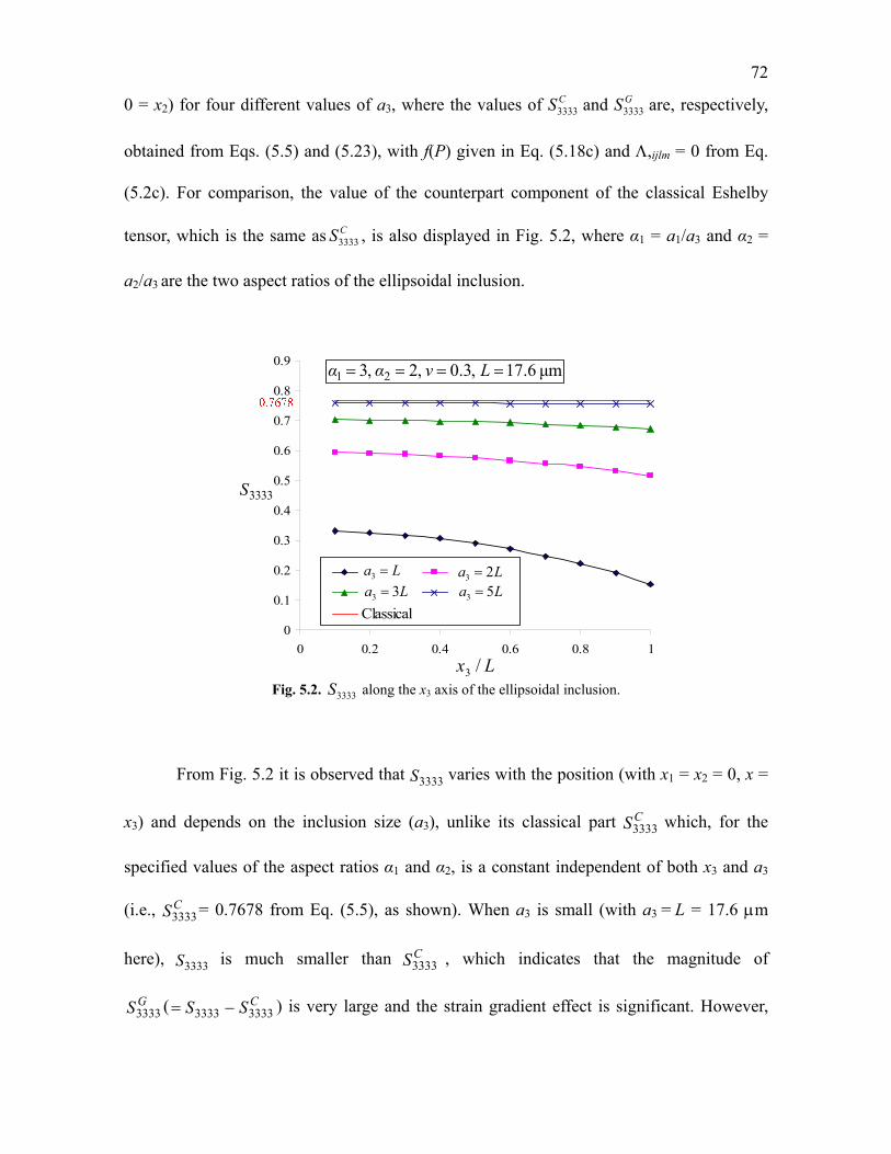
72

0 = x2) for four different values of a3, where the values of CS3333 and

GS3333 are, respectively,

obtained from Eqs. (5.5) and (5.23), with f(P) given in Eq. (5.18c) and ,ijlm = 0 from Eq.

(5.2c). For comparison, the value of the counterpart component of the classical Eshelby

tensor, which is the same as CS3333 , is also displayed in Fig. 5.2, where α1 = a1/a3 and α2 =

a2/a3 are the two aspect ratios of the ellipsoidal inclusion.

0

0.1

0.2

0.3

0.4

0.5

0.6

0.7

0.8

0.9

0 0.2 0.4 0.6 0.8 1

L 2L 3L 5L

Classical

La 3 La 23 La 33 La 53

μm6.17,3.0,2,3 21 Lναα

Lx /3

3333S

Fig. 5.2. 3333S along the x3 axis of the ellipsoidal inclusion.

From Fig. 5.2 it is observed that 3333S varies with the position (with x1 = x2 = 0, x =

x3) and depends on the inclusion size (a3), unlike its classical part CS3333 which, for the

specified values of the aspect ratios α1 and α2, is a constant independent of both x3 and a3

(i.e., CS3333 = 0.7678 from Eq. (5.5), as shown). When a3 is small (with a3 = L = 17.6 m

here), 3333S is much smaller than CS3333 , which indicates that the magnitude of

GS3333 ( CSS 33333333 ) is very large and the strain gradient effect is significant. However,

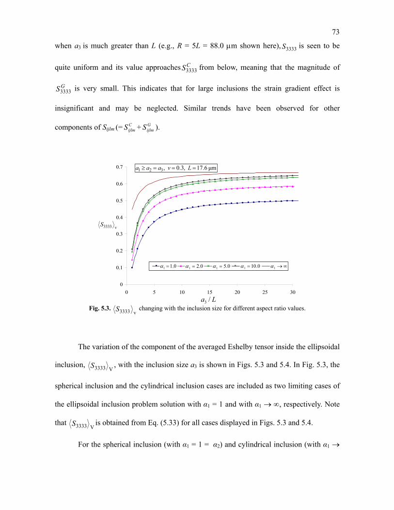
73

when a3 is much greater than L (e.g., R = 5L = 88.0 m shown here), 3333S is seen to be

quite uniform and its value approaches CS3333 from below, meaning that the magnitude of

GS3333 is very small. This indicates that for large inclusions the strain gradient effect is

insignificant and may be neglected. Similar trends have been observed for other

components of Sijlm (=CijlmS + G

ijlmS ).

0

0.1

0.2

0.3

0.4

0.5

0.6

0.7

0 5 10 15 20 25 30

L 2L 5L 10L cylind0.11 0.21 0.51 0.101 1

μm6.17,3.0,321 Lνaaa

La /3

v3333S

Fig. 5.3.

v3333S changing with the inclusion size for different aspect ratio values.

The variation of the component of the averaged Eshelby tensor inside the ellipsoidal

inclusion, V3333S , with the inclusion size a3 is shown in Figs. 5.3 and 5.4. In Fig. 5.3, the

spherical inclusion and the cylindrical inclusion cases are included as two limiting cases of

the ellipsoidal inclusion problem solution with α1 = 1 and with α1 , respectively. Note

that V3333S is obtained from Eq. (5.33) for all cases displayed in Figs. 5.3 and 5.4.

For the spherical inclusion (with α1 = 1 = α2) and cylindrical inclusion (with α1

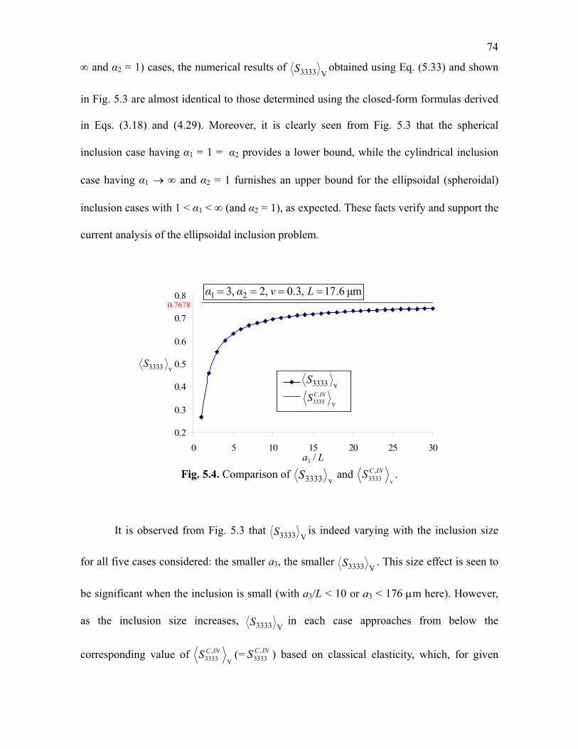
74

and α2 = 1) cases, the numerical results of V3333S obtained using Eq. (5.33) and shown

in Fig. 5.3 are almost identical to those determined using the closed-form formulas derived

in Eqs. (3.18) and (4.29). Moreover, it is clearly seen from Fig. 5.3 that the spherical

inclusion case having α1 = 1 = α2 provides a lower bound, while the cylindrical inclusion

case having α1 and α2 = 1 furnishes an upper bound for the ellipsoidal (spheroidal)

inclusion cases with 1 < α1 < (and α2 = 1), as expected. These facts verify and support the

current analysis of the ellipsoidal inclusion problem.

0.2

0.3

0.4

0.5

0.6

0.7

0.8

0 5 10 15 20 25 30

Grad

class

μm6.17,3.0,2,3 21 Lναα

v3333S

La /3

0.7678

v3333S

V3333INC,S

Fig. 5.4. Comparison of

v3333S and v

,3333

INCS .

It is observed from Fig. 5.3 that V3333S is indeed varying with the inclusion size

for all five cases considered: the smaller a3, the smaller V3333S . This size effect is seen to

be significant when the inclusion is small (with a3/L < 10 or a3 < 176 m here). However,

as the inclusion size increases, V3333S in each case approaches from below the

corresponding value of V

,3333

INCS (= INCS ,3333 ) based on classical elasticity, which, for given

75

values of the aspect ratios, is a constant independent of a3, as discussed in Section 5.2. This

comparison is further illustrated in Fig. 5.4, where it is shown that the classical Eshelby

tensor component, as a constant (i.e., V

,3333

INCS = 0.7678 from Eq. (5.5) for α1 = 3 and α2 =

2), cannot explain the inclusion size effect.

5.4. Summary

The Eshelby problem of an ellipsoidal inclusion (with three distinct semi-axes) in an

infinite homogeneous isotropic elastic material is analytically solved by using a simplified

strain gradient elasticity theory (SSGET) that involves one material length scale parameter.

Analytical expressions for the Eshelby tensor are derived for both the interior and exterior

cases in terms of two line integrals with an unbounded upper limit and two surface integrals

over a unit sphere.

The newly obtained fourth-order Eshelby tensor for each case consists of two parts:

a classical part depending only on Poisson’s ratio, and a gradient part depending on the

length scale parameter additionally. As a result, the new Eshelby tensor based on the

SSGET can capture the inclusion size effect, unlike its classical counterpart. The fourth-

order Eshelby tensor is accompanied by a fifth-order Eshelby-like tensor that links the

eigenstrain gradient to the disturbed strain and contains only a gradient part. In the absence

of the microstructure-dependent strain gradient effect, both the gradient part of the Eshelby

tensor and the Eshelby-like tensor vanish, and the non-classical Eshelby tensor is reduced

to that based on classical elasticity. Moreover, the Eshelby tensors for the spherical and

cylindrical inclusion problems based on the SSGET are included in the current Eshelby

tensor as two limiting cases.

76

In addition, the newly obtained Eshelby tensor inside or outside the ellipsoidal

inclusion depends on the position, differing from the classical Eshelby tensor that is

uniform inside the inclusion. This necessitates the determination of the volume average of

the new Eshelby tensor over the ellipsoidal inclusion needed in homogenization analyses,

which is done analytically in this study.

To further illustrate the newly derived non-classical Eshelby tensor, sample

numerical results are provided. These results reveal that the non-classical Eshelby tensor

varies with both the position and the inclusion size, thereby capturing the size effect at the

micron scale, unlike the classical Eshelby tensor. The components of the averaged Eshelby

tensor are found to decrease as the inclusion size decreases, and these components are

observed to approach (from below) the values of the corresponding components of the

Eshelby tensor based on classical elasticity when the inclusion size is large enough.

77

CHAPTER VI

SOLUTION OF AN ESHELBY-TYPE

INCLUSION PROBLEM WITH A BOUNDED

DOMAIN AND THE ESHELBY TENSOR FOR

A SPHERICAL INCLUSION IN A FINITE

SPHERICAL MATRIX

6.1. Introduction

In the last four chapters, the Eshelby tensor for an inclusion embedded in an infinite

homogeneous isotropic elastic body is obtained using the simplified strain gradient elastic

theory (SSGET). This non-classical Eshelby tensor contains a material length scale

parameter and, therefore, is capable of explaining the microstructure-dependent size effect

in the composites at the micro- or nano- scale. However, both the classical Eshelby tensor

and the newly derived non-classical Eshelby tensor are for an inclusion embedded in an

infinite elastic matrix. This implies that the disturbed displacement due to the inclusion

makes no influence on the displacement at the boundary of the elastic body, and vice versa.

Consequently, these Eshelby tensors and the subsequent homogenization methods cannot

account for the boundary effect of a finite body. Hence, there has been a need to obtain the

Eshelby tensor for an inclusion in a finite matrix subject to traction, displacement or mixed

boundary conditions.

A few analytical studies have been performed using classical elasticity to solve the

problem of an inclusion in a finite homogeneous isotropic elastic body. Kinoshita and Mura

78

(1984) provided the first theoretical study of the finite-domain inclusion problem based on

classical elasticity. They proved the existence and uniqueness of the Neumann tensor for a

bounded homogeneous elastic body, which reduces to the Green’s function (also a second-

order tensor) when the body is unbounded. The use of this Neumann tensor would then lead

to solutions of finite-domain eigenstrain problems. However, the determination of the

Neumann tensor for a bounded elastic body is rather challenging, and only the Neumann

tensor for a half space was given in Kinoshita and Mura (1984). By using a displacement

method in classical elasticity and solving the boundary-value problems directly, Luo and

Weng (1987) determined the elastic field in a spherically concentric three-phase solid

consisting of an inclusion, an interphase layer, and an infinite matrix. The presence of the

finite interphase layer between the inclusion and matrix enabled a modification of the Mori-

Tanaka method, but no explicit expression of Eshelby tensor for the modified problem was

provided there. More recently, Eshelby tensor for a spherical inclusion in a finite spherical

elastic matrix was analytically obtained in Li et al. (2007) by using Somigliana’s identity

and Green’s function for an infinite three-dimensional (3-D) elastic body in classical

elasticity. In contrast, no analytical solution has been provided for the finite-domain

inclusion problem using any higher-order elasticity theory. This motivated the current study.

In the present chapter, a solution for the Eshelby inclusion problem of a finite

homogeneous isotropic elastic body containing an inclusion prescribed with a uniform

eigenstrain and a uniform eigenstrain gradient is first derived in a general form. It makes

use of an extended Betti’s reciprocal theorem and an extended Somigliana’s identity based

on a simplified strain gradient elasticity theory elaborated in Gao and Park (2007), which

involves only one material length scale parameter and has been successfully employed to

obtain analytical solutions of several problems (e.g., Gao and Ma, 2009; Gao et al., 2009;

79

Ma and Gao, 2009). The problem of a spherical inclusion embedded concentrically in a

finite spherical elastic body is then analytically solved by applying the general solution,

with the Eshelby tensor and its volume average derived in closed forms.

The rest of this chapter is organized as follows. In Section 6.2, an extended Betti’s

reciprocal theorem is first proposed and proved. It is then followed by the derivation of a

general solution for the finite-domain Eshelby inclusion problem based on this reciprocal

theorem and an extended Somigliana’s identity that arises subsequently. The finite-domain

spherical inclusion problem is solved in Section 6.3 by using the general formulas derived

in Section 6.2, which leads to closed-form expressions of the Eshelby tensor and its volume

average. In Section 6.4, sample numerical results are presented to quantitatively show how

the components of the Eshelby tensor obtained in Section 6.3 vary with the position,

inclusion size, matrix size, and inclusion volume fraction, where the size and boundary

effects are observed and discussed. The chapter concludes with a summary in Section 6.5.

6.2. Strain Gradient Solution of Eshelby’s Inclusion Problem in a Finite Domain

6.2.1. Extended Betti’s reciprocal theorem

For an elastic body satisfying the SSGET reviewed in Section 2.1, Betti’s first

reciprocal theorem in classical elasticity (e.g., Sadd, 2009) can be extended to

dVdV Iijk

IIijk

Iij

IIij

IIijk

Iijk

IIij

Iij

)()()()()()()()( , (6.1)

where the superscripts “(I)” and “(II)” represent two loading sets, and is the region

occupied by the elastic body.

To prove this extended Betti’s reciprocal theorem based on the SSGET, it is noted

that the second term in the strain energy density function on each side of Eq. (6.1), which is

80

absent in classical elasticity, is required in the SSGET (see Eq. (2.4)). Also,

,

,)()()()(2)()(2)()(

)()()()()()()()(

Imnk

IImnk

Imnk

IIijkmnij

IIijk

Imnkijmn

IIijk

Iijk

Ikl

IIkl

Ikl

IIijklij

IIij

Iklijkl

IIij

Iij

CLCL

CC

(6.2)

where use has been made of Eqs. (2.5a,b) and the major symmetry of the stiffness tensor

(i.e., Cijkl = Cklij). Substituting Eq. (6.2) into the left hand side of Eq. (6.1) will immediately

give the right hand side of Eq. (6.1), thereby proving Eq. (6.1).

Physically, the extended Betti’s theorem expressed in Eq. (6.1) states that the strain

energy in the elastic body induced by the loading set (I) through the displacement field

caused by the loading set (II) is equal to that induced by the loading set (II) through the

displacement field caused by loading set (I).

Using Eqs. (2.5a–d) and (2.7) gives, with the help of the divergence theorem,

dAnuqutdVudV lIIli

Ii

IIi

Ii

IIi

Ijij

IIijk

Iijk

IIij

Iij

)(,

)()()(

Ω

)()(,Ω

)()()()( (6.3)

for any region bounded by a smooth surface (without any edge), where n = niei is

the outward unit normal vector on , and ti and qi are, respectively, the Cauchy traction

and double stress traction defined by (Gao and Park, 2007),

kjijkijllkijkjkijkjiji nnqnnnnnt ,)()( ,, . (6.4a,b)

With the help of Eq. (6.3), Eq. (6.1) can be rewritten as

.)(,

)()()()()(,

)(,

)()()()()(, dAnuqutdVudAnuqutdVu l

Ili

IIi

Ii

IIi

Ii

IIjijl

IIli

Ii

IIi

Ii

IIi

Ijij

(6.5)

Eq. (6.5), as the extended Betti’s second reciprocal theorem based on the SSGET, will be

directly used to derive the solution of the finite-domain inclusion problem next.

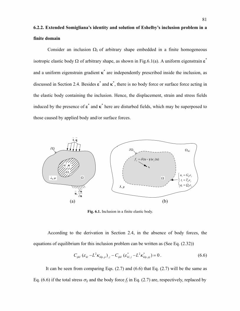
81

6.2.2. Extended Somigliana’s identity and solution of Eshelby’s inclusion problem in a

finite domain

Consider an inclusion I of arbitrary shape embedded in a finite homogeneous

isotropic elastic body of arbitrary shape, as shown in Fig.6.1(a). A uniform eigenstrain *

and a uniform eigenstrain gradient * are independently prescribed inside the inclusion, as

discussed in Section 2.4. Besides * and *, there is no body force or surface force acting in

the elastic body containing the inclusion. Hence, the displacement, strain and stress fields

induced by the presence of * and * here are disturbed fields, which may be superposed to

those caused by applied body and/or surface forces.

**,κε

I

n

uu

,

qt,

jiji

jiji

jiji

eQq

eTt

eGu

)()( xyx jj ef

(a) (b)

Fig. 6.1. Inclusion in a finite elastic body.

According to the derivation in Section 2.4, in the absence of body forces, the

equations of equilibrium for this inclusion problem can be written as (See Eq. (2.32))

0)()( *,

2*,,,

2 pjklpjklijkljpklpklijkl LCLC . (6.6)

It can be seen from comparing Eqs. (2.7) and (6.6) that Eq. (2.7) will be the same as

Eq. (6.6) if the total stress ij and the body force fj in Eq. (2.7) are, respectively, replaced by

82

)( ,2

pklpklijklij LC , (6.7)

)( *,

2*, pjklpjklijkli LCf . (6.8)

The total stress expression listed in Eq. (6.7) is exactly what is given by Eqs. (2.5a,b)

and (2.7). Hence, Eqs. (2.7), (6.7) and (6.8) can be used as an alternative to the equilibrium

equations provided in Eq. (6.6).

On the other hand, consider an infinite homogeneous isotropic elastic body ∞

subject to a unit concentrated body force applied at point x, as shown in Fig.6.1(b).

Substituting the special body force fi(y) = (x y)ei(x) into Eq. (2.7), leads to the

equilibrium equations for this point-force problem as

0)()()(, xyxy ijij e , (6.9)

where )( yx is the 3-D Dirac delta function, and )(xie is the ith component of the unit

force. Note that the Green’s function )( yxG in the SSGET, given in Eq. (2.28) and (2.29)

is a second-order tensor whose component )( yx ijG represents the displacement

component ui at point y in a 3-D infinite elastic body due to a unit concentrated body force

applied at point x in the body in the jth direction. That is, )( yx ijG (= )( yx jiG ) satisfies

the equilibrium equations in Eq. (6.9). Actually, the use of this Green’s function will give

the solution of the this concentrated-force problem based on the SSGET for the

displacement, stress, traction and double stress traction at point y in the 3-D infinite elastic

body due to the unit concentrated body force applied at point x (see Eqs. (6.11a–c)).

The complete boundary conditions in the SSGET have been derived in Gao and

Park (2007) using a variational formulation. Two typical kinds of such boundary conditions

are the Dirichlet-like boundary conditions:

83

on, , n

unuuu i

lliii , (6.10a)

i.e., the displacement and displacement gradient are specified on the smooth boundary ,

and the Neumann-like boundary conditions:

on, iiii qqtt , (6.10b)

i.e., the Cauchy traction and double stress traction are specified on . For the inclusion

problem under consideration, the disturbed displacement, strain and stress fields due to *

and * can be obtained by setting the prescribed field quantities on to zero (i.e., using

homogeneous boundary conditions), as was done in Li et al. (2007) in the context of

classical elasticity.

To solve the finite-domain inclusion problem satisfying Eqs. (6.6) and (6.10a) or

Eqs. (6.6) and (6.10b), the extended Betti’s theorem expressed in Eq. (6.5) can be used. The

loading by * and * in the current inclusion problem shown Fig. 6.1(a) is taken to be the

loading set (II), while that by a unit concentrated body force applied at a point inside a

finite elastic body identical to that of (see Fig. 6.1(b)) as the loading set (I). For the latter,

the finite elastic body is cut out of an infinite body ∞ having the same elastic properties (

and ), and the displacement, Cauchy traction and double stress traction at any point y on

the boundary (cutting surface) are respectively given by

)()()( xyxy jiji eGu , (6.11a)

)()()( xyxy jiji eTt , (6.11b)

)()()( xyxy jiji eQq , (6.11c)

where Gij(x y) is the 3-D Green’s function based on the SSGET listed in Eq. (2.28), and

Tij(x y) and Qij(x y) are, respectively, the second-order Cauchy traction and double

stress traction transformation tensors related to the Green’s function Gij(x y), which lead

84

to, respectively, the traction and double stress traction in the ith direction at point y due to

the unit concentrated body force applied in the jth direction at point x. The expressions of

Tij(x y) and Qij(x y) based on the SSGET can be obtained from Eqs. (6.11a), (2.5a–d)

(2.7) and (6.4a,b) as (see Appendix F)

),)](2(

)([)1(32

])2(

)2()2()([

])()()([)1(32

)2()()1(32

1

,,,,,,

,,

2

,,,

,2

,2

,,,2

,2

,,,,,,2

2

,,,,,

jllpjllpjpijkpikjpjkip

ijkpmmlpjjplikiklpkipl

pikpikpipkjijkikjki

lpikplmmpikpmmikmm

jijkjikjkiikmmik

nnnnnnnBAA

BAv

LnnnBAnnnA

nBAAnBAnA

nnnBAnBAnBAv

L

nBnAnAnBAv

T

(6.12a)

,)2()()1(32 ,,,,,

2

pjijkpikjpjkipijkpmmik nnBAABAv

LQ

(6.12b)

where A = A(r) and B = B(r) are defined in Eqs. (2.29). When L = 0, Tik and Qik in Eqs.

(6.12a,b) reduce to

,0,3

)12())(21()1(8

123

C

ikki

ikjjkiikC

ik Qr

rrvnrnrnrv

rvT

(6.12c,d)

which are the traction transformation tensors based on classical elasticity. It can be readily

shown that Eq. (6.12c) is the same as that provided in Paris and Canas (1997) (see Eq.

(5.4.20) there).

Using Eqs. (2.7), (6.7–6.9) and (6.11a–c) in Eq. (6.5) yields, with the help of the

divergence theorem, the disturbed displacement field at any point x for the finite

domain inclusion problem as

,)()()(

)()()()()(

)()()()()(

)(,

)(

)(,

)(

*,

2*,

)(

ylII

ilimII

iim

ylIIliim

IIiim

yklpjpimkljimijklII

m

dAnqGtG

dAnuQuT

dVGLGCu

yyxyx

yyyxyyx

yyxyyxx

(6.13)

85

where the derivatives are with respective to y (the integration variable), and use has been

made of the fact that the eigenstrain and eigenstrain gradient vanish on the boundary of the

finite body , which is outside the inclusion. It is seen from Eq. (6.13) that the

displacement contains contributions from field quantities distributed both in the volume

and on its surface . If the two surface integrals in Eq. (6.13) are suppressed, the

disturbed displacement field given in Eq. (6.13) reduces to that for the problem of an

inclusion in an infinite elastic body based on the SSGET (see Eq. (2.34)). This means that

the two surface integrals in Eq. (6.13) represent the boundary effect due to the finite size of

the elastic body and/or the constraints existing on the finite boundary. Eq. (6.13) can be

viewed as an extended Somigliana’s identity based on the SSGET, which plays a role

similar to that of the Somigliana’s identity in classical elasticity (e.g., Paris and Canas,

1997; Sadd, 2009).

Furthermore, if the microstructure-dependent strain gradient effect is neglected by

setting L = 0, the higher-order terms involved in Eq. (6.13) vanish (with ijk = 0, qi = 0 and

Qij = 0 from Eqs. (2.5b), (6.4b) and (6.12b), respectively), and Eq. (6.13) reduces to

,)()()()()()( )()(*,

)(y

IIi

Cim

IIi

Cimykl

Cjimijkl

IIm dAtGuTdVGCu

yxyyxyyxx (6.14)

where CijG is the Green’s function for a 3-D infinite elastic body in classical elasticity listed

in Eq. (2.23), jCim

Cjim yGG /)(, yx , C

imT is the classical Cauchy traction transformation

tenor given in Eq. (6.12c), and )( IIit is the traction related to the Cauchy stress )( II

ij by

jII

ijII

i nt )()( . It can be readily verified that Eq. (6.14) is the same as the Somigliana’s

identity in classical elasticity used by Li et.al. (2007).

Now, with 0,0

n

uu i

i on for the loading set (II), it follows from Eqs. (6.10a)

86

and (6.13) that

,)()()(

)()()()()(

)(,

)(

*,

2*,

)(

ylII

ilimII

iim

yklpjpimkljimijklII

m

dAnqGtG

dVGLGCu

yyxyx

yyxyyxx (6.15)

which is the disturbed displacement field in the finite elastic body subject to the

homogeneous Dirichlet-like boundary conditions. Similarly, using Eq. (6.10b) in Eq. (6.13)

gives, with 0,0 ii qt on for the loading set (II),

,)()()()()(

)()()()()(

)(,

)(

*,

2*,

)(

ylIIliim

IIiim

yklpjpimkljimijklII

m

dAnuQuT

dVGLGCu

yyyxyyx

yyxyyxx (6.16)

which is the disturbed displacement field in the finite elastic body subject to the

homogeneous Neumann-like boundary conditions.

Clearly, Eqs. (6.15) and (6.16) are integral equations that involve the unknown

displacement components in the integrands of the surface integrals. It is very challenging to

obtain analytical solutions of such integral equations even for inclusion problems involving

simple-shape elastic bodies and inclusions. Hence, only the inclusion problems defined in

Eq. (6.15), which are associated with the simpler Dirichlet-like boundary conditions, will

continue to be formulated in the rest of this section.

As stated earlier, the derivatives involved in the integrals in Eqs. (6.13)–(6.16) are

with respect to y, which is the integration variable. Note that

k

ij

k

ij

x

G

y

G

)()( yxyx. (6.17)

Using Eq. (6.17) in Eq. (6.15) then gives

.)()()(

)()()()()(

)(,

)(

*,

2*,

)(

ylII

ilimII

iim

yklpjpimkljimijklII

m

dAnqGtG

dVGLGCu

yyxyx

yyxyyxx (6.18)

87

In Eq. (6.18) and all of the ensuing equations, the derivatives are taken with respect to x

unless otherwise stated.

Substituting Eq. (6.18) into Eq. (2.5c) yields the disturbed strain as

,)()(2

1

)()(2

1)(

,,,,

*,,

2*,,

ylilminlnimiminnim

yklpjpminjpnimkljminjnimijklmn

dAnqGGtGG

dVGGLGGC

x (6.19)

where the surface integral term represents the boundary effect on the disturbed strain field

for the finite-domain inclusion problem. Note that in Eq. (6.19) and other subsequent

equations, the superscript “(II)” is dropped for convenience, since the strain, traction and

double stress traction involved in Eq. (6.19) and ensuing equations are all for the inclusion

problem under the loading set (II) shown in Fig. 6.1(a).

For uniform * and *, the volume integral term in Eq. (6.19) represents the

disturbed strain field in an infinite (unbounded) elastic body containing the inclusion (see

Eq. (2.34)), which can be written as

*,*,)( klpmnklpklmnklmn TS x , (6.20a)

,)(2

1,,

, yjminjnimijklmnkl dVGGCS (6.20b)

,)(2 ,,

2, yjpminjpnimijklmnklp dVGGC

LT (6.20c)

where ,mnklS and ,

mnklpT , as defined, are, respectively, the fourth-order Eshelby tensor and the

fifth-order Eshelby-like (gradient) tenor for the unbounded-domain inclusion problem, and

the superscript “ ” can be either “I”, representing the interior case with x located inside the

inclusion, or “E”, representing the exterior case with x located outside the inclusion.

Based on Eqs. (6.20a–c) and the similarity between the unbounded and bounded

cases, it is postulated that for the present bounded-domain inclusion problem the disturbed

88

strain field has the following form:

*,*, )()()( klpF

mnklpklF

mnklmn TS xxx , (6.21)

which is similar to the one given in Eqs. (6.20a–c) for the unbounded-domain inclusion

problem. In Eq. (6.21), Fmnklp

Fmnkl TS ,, and, denote, respectively, the Eshelby tensor and the

Eshelby-like tensor for the current finite-domain inclusion problem.

Using Eqs. (2.5a,b), (2.7) and (6.21) in Eqs. (6.4a,b) gives

**mnrimnrmnimni fgt , **

mnrimnrmnimni thq , (6.22a,b)

where

],)()()1[( ,,

,2

,,

,2,22

jqqpF

pklmnjpF

pklmnjF

klmnijklimn nnnSLnSLnSLCg (6.23a)

])()()1[( ,,

,2

,,

,2,22

jqqpF

pklmnrjpF

pklmnrjF

klmnrijklimnr nnnTLnTLnTLCf , (6.23b)

pjpF

klmnijklimn nnSCLh ,,2 , (6.23c)

pjpF

klmnrijklimnr nnTCLt ,,2 . (6.23d)

Substituting Eqs. (6.20a–c), (6.21) and (6.22a,b) into Eq. (6.19) then yields

.)()(2

1,,

**

Ω ,,**

*,*,*,*,

yqqminqnimklpiklpkliklminnimklpiklpklikl

klpmnklpklmnklklpF

mnklpklF

mnkl

dAnGGthGGfg

TSTS

(6.24)

From Eq. (6.24) it follows that

,,,, FBmnklmnkl

Fmnkl SSS FB

mnklpmnklpF

mnklp TTT ,,, , (6.25a,b)

where

yqqminqnimiklminnimiklFB

mnkl dAnGGhGGgS )()(

2

1,,,,

, , (6.26a)

yqqminqnimiklpminnimiklpFB

mnklp dAnGGtGGfT )()(

2

1,,,,

, . (6.26b)

89

Here FBmnklS , and FB

mnklpT , can be regarded, respectively, as the boundary parts of the finite-

domain Eshelby tensor and Eshelby-like tensor. In the absence of the boundary effect,

FBmnklS , = 0, FB

mnklpT , = 0, and FmnklS , and F

mnklpT , reduce, respectively, to their counterparts ,mnklS and

,mnklpT for the unbounded-domain inclusion problem, as shown in Eqs. (6.25a,b).

Clearly, Eqs. (6.25a,b), (6.26a,b) and (6.23a-d) define the integral equations to solve

for FmnklS , and F

mnklpT , , which depend on the shape and size of both the elastic body (through

the surface integrals listed in Eqs. (6.26a,b)) and the inclusion (via ,mnklS and ,

mnklpT ). Hence,

closed-form solutions may be derived only for problems involving simple-shape finite

elastic bodies and inclusions. The spherical inclusion problem to be discussed next is one of

such problems that have been solved analytically.

6.3. Eshelby Tensor for a Finite-Domain Spherical Inclusion Problem

6.3.1. Position-dependent Eshelby tensor

Consider a finite spherical elastic body of radius H containing a concentric

spherical inclusion I of radius R, as illustrated in Fig. 6.2.

** κ,ε

Fig. 6.2. Spherical Inclusion in a finite spherical elastic body.

90

For the unbounded spherical inclusion problem, the Eshelby tensor inside the

inclusion based on the SSGET, which is derived in obtained in Section 3.2, can be written

as

)()( ,,, xx GImnkl

CImnkl

Imnkl SSS , (6.27)

where x is a point located inside the inclusion (i.e., x I or 0 < |x| < R), CImnklS , is the

classical part that is uniform for all x I, and )(, xGImnklS is the gradient part that varies with

the position of point x. It can be readily shown that ,ImnklS obtained in Eqs. (3.4) – (3.7a–f)

and involved in Eq. (6.27) can be written in a matrix form as

)]([)]([)( ,0, xSS ITmnkl

Imnkl

xx, (6.28)

where

],,

,,,,[)]([000000000000

0000T0

lknmkmnllmnkknmllnmk

nmkllkmnnkmlnlmkklmnmnkl

xxxxxxxxxxxx

xxxx

x (6.29a)

)]([][)]([ ,,, xSSxS GICII , (6.29b)

,0,0,0,0,)1(15

54,

)1(15

15][ ,

T

CIS

(6.29c)

,,,,,,)]([ ,6

,5

,4

,3

,2

,1

, TGIGIGIGIGIGIGI SSSSSSxS (6.29d)

with

,)Λ(Γ21

31)Λ(Γ

21Γ

21

)1(2

)1(4

12

23

221

,1

DL

v

vDxL

v

vD

v

vv

vS GI

(6.30a)

,)Λ(ΓΓ)1()1(4

12

21

,2

DLDv

vS GI

(6.30b)

,)Λ(Γ21

51)Λ(Γ

21Γ

21

)1(2

)1(4 32

422

2

2,

3

DL

v

vDxL

v

vD

v

vv

v

xS GI

(6.30c)

),Λ(Γ)1(4 3

22,

4

Dv

xLS GI

(6.31d)

91

,)Λ(Γ2Γ)1()1(8 3

22

2,

5

DLDvv

xS GI

(6.30e)

).Λ(Γ)1(4 4

42,

6

Dv

xLS GI

(6.30f)

The differentials 4321 ,,, DDDD and 4321 ,,, DDDD involved in Eqs. (6.30a–

f) are given by Eq. (3.10). In Eq. (6.29a) and throughout this dissertation, xxx ii /0 is the

ith component of the unit vector x0 = x/x, and mm xxx x is the distance from point x

to the center of the spherical body that serves as the origin of the coordinate system.

For the unbounded spherical inclusion problem, the Eshelby tensor outside the

inclusion based on the SSGET has been obtained in Section 3.2 and is summarized here,

)()()( ,,, xxx GEmnkl

CEmnkl

Emnkl SSS , (6.31)

where x is a point located outside the inclusion (i.e., x I or R < |x| < H), )(, xCEmnklS is the

classical part, and )(, xGEmnklS is the gradient part. Both CE

mnklS , and GEmnklS , vary with the position of

x in this exterior case, unlike in the interior case. In a matrix form, Eq. (6.31) can be written

as

)],([)]([)( ,0, xSS ETmnkl

Emnkl

xx (6.32)

where Tmnkl )]([ 0x is the same as that defined in Eq. (6.29a), and

)],([)]([)]([ ,,, xSxSxS GECEE (6.33)

in which

92

,75105,1515,15)21(15

,1515),21(53),21(53)1(30

1)]([

222

2223,

T

CE

x

R

x

Rv

x

Rv

x

Rv

x

Rv

x

R

x

R

vxS

(6.34a)

TGEGEGEGEGEGEGE SSSSSSxS ,6

,5

,4

,3

,2

,1

, ,,,,,)( , (6.34b)

with GES ,1 – GES ,

6 obtainable from using Eq. (3.20) in their interior counterparts GIS ,1 –

GIS ,6 given in Eqs. (6.30a–f).

Based on the similarity between the unbounded- and bounded-domain inclusion

problems and the forms of the Eshelby tensor for the unbounded-domain problem given in

Eqs. (6.28) and (6.32), it is postulated that the Eshelby tensor for the current bounded-

domain spherical inclusion problem can be expressed in a similar form as

)]([)]([)( ,0, xSS FTmnkl

Fmnkl

xx , (6.35)

where Tmnkl )]([ 0x is the same as that defined in Eq. (6.29a), and

TFFFFFFF xSxSxSxSxSxSxS )(),(),(),(),(),()]([ ,6

,5

,4

,3

,2

,1

, (6.36)

is an array of six components yet to be determined.

Using Eq. (6.35) in Eqs. (6.23a,b) yields, after carrying out the algebra,

)(, HSg FEiklikl , 0iklh , (6.37a,b)

on , where

Tlkikillikiklikl Mnnnnnn ,, , (6.38)

93

T

TM

)143(224)2(2

)61)((4)21(28

0082

)61)(23(0)23(2

022

0023

, (6.39)

with 22 / HL , and being the Lamé constants, yyn ii / being the ith component of

the unit vector n representing the direction of y, and mm yyy y .

Using Eqs. (6.37a,b)–(6.39) in Eq. (6.26a) gives the boundary part of the finite-

domain Eshelby tensor, in a matrix form, as

)(,,2

1 ,321

, HSMQQQS FETFBmnkl , (6.40)

where

,)(

,))((,)(

,,3

,,2,,1

yminnimlki

yminnimkillikyminnimikl

dAGGnnnQ

dAGGnnQdAGGnQ (6.41)

with ijG , given in Eqs. (2.28) and (2.29), being the 3-D Green’s function for an infinite

elastic body based on the SSGET. The use of Eqs. (2.28) and (2.29) in Eq. (6.41) results in

imninmmnkl BnAnAnQ

,,,1 2 , (6.42a)

lmnkkmnlmklnnklmmlknnlkm BnBnAnAnAnAnQ,,,,,,2 22 (6.42b)

imnlki

mlkn

nlkm nnnBnnnAnnnAQ

,,,3 2 , (6.42c)

where

L

r

L

r

er

L

r

Lr

vrBe

rrA

22 22

)1(16

1)(,1

1

4

1)(

, (6.43a,b)

with yx r . In Eqs. (6.42a–c) and in the sequel, f denotes the surface integral of

function f over ∂Ω (i.e., the surface of the spherical elastic body of radius H) defined by

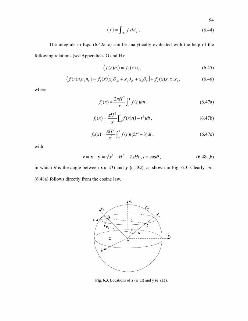
94

ydAff . (6.44)

The integrals in Eqs. (6.42a–c) can be analytically evaluated with the help of the

following relations (see Appendices G and H):

ii xxfnrf )()( 0 , (6.45)

kjiijkikjjkikji xxxxfxxxxfnnnrf )()()( 21 , (6.46)

where

1

1

2

0 )(2

)( tdtrfx

Hxf

, (6.47a)

1

1

22

1 )1()()( dtttrfx

Hxf

, (6.47b)

1

1

23

2

2 )35()()( dtttrfx

Hxf

, (6.47c)

with

xHtHxr 222 yx , t cos , (6.48a,b)

in which is the angle between x ( ) and y ( ), as shown in Fig. 6.3. Clearly, Eq.

(6.48a) follows directly from the cosine law.

1e

2e

3e

2e

3e

1e

Fig. 6.3. Locations of x ( ) and y ( ).

95

Applying Eqs. (6.45) and (6.47a) to )(rA and )(rB defined in Eqs. (6.43a,b),

respectively, yields, together with Eq. (6.44),

,)()( 0 ii xxAnrA ii xxBnrB )()( 0 , (6.49a,b)

where

3

10

)(

3

1)(

x

xxA

, 3

12222

0 )1(2

)(

)1(60

105)(

xv

xL

v

LHxxB

, (6.50a,b)

with

)]/cosh()/sinh()[()( /1 LxxLxLLHLex LH . (6.51)

Similarly, the application of Eqs. (6.46) and (6.47b,c) to )(rA and )(rB respectively results

in

,)()()(

,)()()(

21

21

kjiijkikjjkikji

kjiijkikjjkikji

xxxxBxxxxBnnnrB

xxxxAxxxxAnnnrA

(6.52a,b)

where

),(1

105

73)( 2522

22

1 xxHH

HxxA

)()1(2

])3(6)2(21[)1(1260

1)( 252

24222222

21 xxHv

LxHLxLHH

HvxB

,

)(1

7

1)( 37222 x

xHHxA

,

)()1(2)1(1260

9590)( 372

2

2

222

2 xxHv

L

Hv

HxLxB

,

,)]/cosh()/sinh([)]/cosh()/sinh()[(45

)/sinh(7)]/cosh()()/sinh([3

)]/cosh()/sinh()[(18)(

2225

22322333

22224/2

LxxLxHxHLLxxLxLHLL

LxxHLLxHxLxHxLxLHL

LxxHLxHxLxLHLex LH

.)]/cosh()/sinh([6)]/cosh()/sinh()[(225

)/sinh(36)]/cosh()()/sinh([15

)/cosh()]/cosh()/sinh()[(90)(

2225

22322333

3322224/3

LxxLxHxHLLxxLxLHLL

LxxHLLxHxLxHxLxLHL

LxLxHLxxHLxHxLxLHLex LH

(6.53a–f )

Using Eqs. (6.49a,b)–(6.53a–f) in Eqs. (5.42a–c) then leads to, in a matrix form,

96

TT

mnkl xQQQQ )]([)(,, 0321 x , (6.54)

where )( 0xmnkl T is the same as that given in Eq. (6.29a), and [Q(x)] is a 3 by 6 matrix

whose components are given by

),2Χ(2

),4Χ2(),2Ζ(2

),X2(2),2Χ(2),2Ζ(2

,4),4(

,,4,42,4

,0),Ν(2),Ν(2

132214

36

1211122

35122112

34

11222

3311132111131

034

2602012

25

2324022

23010220121

161513122012

141011

BDDADxQ

BDDADAxQBDDADxQ

DBDAxQBDAQBDDAQ

BDxQBDADxQ

QQBDxQBDAQBDQ

QQQQDADxQDAQ

(6.55)

with

00 3)( BBxx , 11 3)( BBxx , 22 5)( BBxx . (6.56)

The differential operators D1(·), D2(·) and D3(·) involved in Eq. (6.55) are defined in Eq.

(3.3).

Substituting Eq. (6.54) into Eq. (6.40) then yields the boundary part of the finite-

domain Eshelby tensor as

)()()(2

1)( ,0, HSMxQS FETTT

mnklFB

mnkl xx , (6.57)

where [Q(x)] is the 3 by 6 matrix whose components are listed in Eq. (6.55), [M] is given in

Eq. (6.39), and )]([ , HS FE can be determined as follows.

Note that Eq. (6.57) can be rewritten as

)()()()( ,0, HSxKS FET

mnklFB

mnkl xx , (6.58)

where

TT MxQxK ][)]([2

1)]([ (6.59)

is a six by six matrix. Using Eqs. (6.28), (6.32), (6.35) and (6.58) in Eq. (6.25a) gives,

97

noting that the six components of )( 0xmnkl are linearly independent,

)]()][([)]([)]([ ,,, HSxKxSxS FEIFI (6.60)

for the interior case with 0 < x < R, and

)]([)]([)]([)]([ ,,, HSxKxSxS FEEFE (6.61)

for the exterior case with R < x < H. By setting x H, Eq. (6.61) gives

)]([)](I[)]([ ,1, HSHKHS EFE , (6.62)

where [I] is the six by six identity matrix, [K(H)] is obtainable from Eq. (6.59) with x = H,

and )]([ , HS E can be determined from Eq. (6.33) with x = H.

Finally, it follows from Eqs. (6.62), (6.60), (6.29b) and (6.35) that the Eshelby

tensor inside the spherical inclusion for the finite-domain inclusion problem can be

expressed as

)]([)]([][)]([)( ,,,0, xSxSSS FBGICITmnkl

FImnkl xx , (6.63)

)]([)](I[)]([)]([ ,1, HSHKxKxS EFB , (6.64)

where x I, 0 < x < R, and [SI,C], [SI,G] and [SB,F] are, respectively, the classical, gradient

and boundary parts of the interior Eshelby tensor based on the SSGET. Note that [SI,C], as

given in Eq. (6.29c), is uniform inside the inclusion, while [SI,G], as listed in Eqs. (6.29d)

and (6.30a–f), depends on L, R and x in a complicated manner. In addition, [SB,F] given in

Eq. (6.64) varies with L, R, H and x. That is, [SB,F] is non-uniform inside the inclusion and

is different for the elastic body with different body and/or inclusion sizes (i.e., with varying

H and/or R) and different materials (with changing L).

98

6.3.2. Volume averaged Eshelby tensor

Considering that the finite-domain Eshelby tensor SI,F is position-dependent inside

the inclusion, the volume average of SI,F over the spherical inclusion will be needed in

predicting effective properties of a heterogeneous particle-reinforced composite. Hence, the

volume average of SI,F is evaluated here.

The volume average of a sufficiently smooth function F(x) over the spherical

inclusion occupying the region I is defined in Eq. (3.11). Replacing F(x) in Eq. (3.11)

with )(, xFImnklS given in Eq. (6.63) then leads to, with the help of Eqs. (3.11) and (6.29a),

V

,

V

,

V

, FBmnkl

Imnkl

FImnkl SSS , (6.65)

where the volume averaged Eshelby tensor for the unbounded spherical inclusion problem

has been obtained in a closed-form in Eq. (3.16). And the volume averaged boundary part

of the Eshelby tensor for the bounded spherical inclusion problem is given by

)(),,(),,( 21V

,nkmlnlmkklmn

FBmnkl HLRSHLRSS , (6.66)

with

FBFBFBFB SSSS

RHLRS ,

6,

4,

3,

131 5

13

1),,( , (6.67a)

FBFBFB SSS

RHLRS ,

6,

5,

232 5

123

1),,( , (6.67b)

R FB

nFB

n dxxSxS0

,2, )( . (6.67c)

Note that )(, xS FBn (n = 1, 2, …, 6) in Eq. (6.67c) is the nth component of the array [SB,F(x)]

given in Eq. (6.64).

By following a similar procedure, the volume average of the fifth-order Eshelby-

like tensor FImnklpT , over the spherical inclusion can also be evaluated, which gives

99

0V

, FImnklpT . It then follows from Eqs. (5.21) and (3.11) that

,*

V

,

V klFI

mnklmn S (6.68)

where V

,FImnklS is given in Eq. (6.65) along with Eqs. (6.67a–c). Equation (6.68) shows that

the average disturbed strain is only related to the eigenstrain * even in the presence of the

eigenstrain gradient *. This result will have important applications in homogenization

analyses.

6.4. Numerical Results

To demonstrate how the components of the Eshelby tensor for the finite-domain

spherical inclusion problem derived in Section 6.3 quantitatively change with the position x,

inclusion size R and matrix size H, some numerical results are provided in this section. In

the numerical analysis presented here, the Poisson’s ratio v is taken to be 0.3, and the

material length scale parameter L to be 17.6 m.

Figure 6.4 shows the distribution of )( ,1111

,1111

,1111

,1111

FBGICIFI SSSS along the x1 axis (or

any radial direction due to the spherical symmetry) of a spherical inclusion concentrically

embedded in a finite spherical elastic matrix. The values of FIS ,1111 displayed in Fig. 6.4 are

obtained from Eqs. (6.63), (6.64), (6.29a,c,d) and (6.30a–f) while those of ,1111IS are

determined from Eqs. (6.28) and (6.29a–j). The inclusion has a fixed size of R = L, while

the matrix domain has three different sizes: H = 2R, H = 3R, and H = 5R, as indicated in Fig.

6.4, where the distribution of )( ,1111

,1111

,1111

GICII SSS for the unbounded spherical inclusion

problem along the same direction is also plotted for comparison. Note that CIS ,1111 is a

constant (i.e., CIS ,1111 = 0.5238 from Eqs. (6.28) and (6.29a–c)).

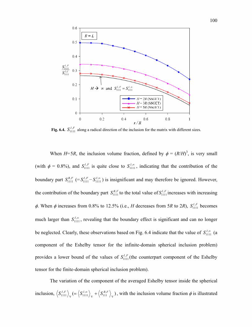
100

CI

FI

S

S,

1111

,1111

,1111

,1111

IFI SS

Fig. 6.4. FIS ,

1111 along a radical direction of the inclusion for the matrix with different sizes.

When H=5R, the inclusion volume fraction, defined by = (R/H)3, is very small

(with = 0.8%), and FIS ,1111 is quite close to ,

1111IS , indicating that the contribution of the

boundary part FBS ,1111 (= FIS ,

1111−,

1111IS ) is insignificant and may therefore be ignored. However,

the contribution of the boundary part FBS ,1111 to the total value of FIS ,

1111 increases with increasing

. When increases from 0.8% to 12.5% (i.e., H decreases from 5R to 2R), FIS ,1111 becomes

much larger than ,1111IS , revealing that the boundary effect is significant and can no longer

be neglected. Clearly, these observations based on Fig. 6.4 indicate that the value of ,1111IS (a

component of the Eshelby tensor for the infinite-domain spherical inclusion problem)

provides a lower bound of the values of FIS ,1111 (the counterpart component of the Eshelby

tensor for the finite-domain spherical inclusion problem).

The variation of the component of the averaged Eshelby tensor inside the spherical

inclusion, )(V

,111V

,1111V

,1111

FBIFI SSS , with the inclusion volume fraction is illustrated

101

in Fig. 6.5. The values of V

,1111IS based on the SSGET for the unbounded spherical

inclusion problem and those of V

,1111

FIS based on classical elasticity for the finite-domain

spherical inclusion problem are also displayed in Fig. 6.5 for comparison. Note that the

values of V

,1111

FIS shown in Fig. 6.5 are obtained from Eqs. (6.65), (3.16), (6.66) and

(6.67a–c), with those for the classical elasticity-based cases determined by setting L 0.

From Eq. (3.16) it is seen that V

,1111IS based on the SSGET is independent of H and is

therefore the same for all of the SSGET-based V

,1111

FIS curves with different values of

shown in Fig. 6.5 (including the curve with 0 or H ). Therefore, the distance

between a line for V

,1111

FIS with a specified ( 0) and the line for V

,1111IS with 0,

based on either the SSGET or classical elasticity, are actually the boundary part V

,111

FBS (=

V

,1111

FIS V

,1111IS ) (see Eq. (6.65)).

Figure 6.5 shows that the inclusion size effect is predicted by the current finite-

domain inclusion problem solution based on the SSGET – unbounded (with 0) and

bounded (with different values of 0). That is, in each case with a fixed inclusion volume

fraction , the smaller the inclusion radius R is, the smaller the value of V

,1111

FIS is. This

size effect is seen to be more significant for the cases with small inclusion volume fractions,

where the boundary effect is small, as will be discussed below. However, as the inclusion

size becomes large (with R > 264 m or R/L > 15 for = 12.5% here), the size effect is

seen to be diminishing. In contrast, the solution based on classical elasticity gives a

constant value of V

,1111

FIS for each value of , which provides an upper bound of the values

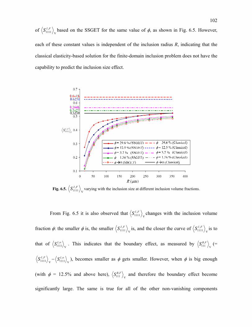
102

of V

,1111

FIS based on the SSGET for the same value of , as shown in Fig. 6.5. However,

each of these constant values is independent of the inclusion radius R, indicating that the

classical elasticity-based solution for the finite-domain inclusion problem does not have the

capability to predict the inclusion size effect.

V

FIS ,1111

Fig. 6.5.

V

,1111

FIS varying with the inclusion size at different inclusion volume fractions.

From Fig. 6.5 it is also observed that V

,1111

FIS changes with the inclusion volume

fraction : the smaller is, the smaller V

,1111

FIS is, and the closer the curve of V

,1111

FIS is to

that of V

,1111IS . This indicates that the boundary effect, as measured by

V

,111

FBS (=

V

,1111

FIS V

,1111IS ), becomes smaller as gets smaller. However, when is big enough

(with = 12.5% and above here), V

,111

FBS and therefore the boundary effect become

significantly large. The same is true for all of the other non-vanishing components

103

ofV

,FImnklS , which is dictated by Eqs. (6.66) and (6.67a–c). These observations indicate that

the boundary effect is insignificant and may be neglected only when inclusion volume

fraction is sufficiently low. In addition, the numerical results reveal that the average

Eshelby tensor for the finite-domain spherical inclusion problem is bounded from below by

the average Eshelby tensor based on the SSGET for the infinite-domain spherical inclusion

problem and is bounded from above by the average Eshelby tensor based on classical

elasticity for the same inclusion problem.

6.5. Summary

An Eshelby-type inclusion problem of a finite elastic body of arbitrary shape

containing an arbitrarily-shaped inclusion prescribed with a uniform eigenstrain and a

uniform eigenstrain gradient is solved using an extended Betti’s reciprocal theorem and an

extended Somigliana’s identity based on a simplified strain gradient elasticity theory

(SSGET), which are proposed and proved in this chapter. The solution for the displacement

field in the bounded elastic body induced by the eigenstrain and eigenstrain gradient is

obtained in a general form in terms of the Green’s function for the unbounded 3-D elastic

medium based on the SSGET. This solution recovers that for the unbounded-domain

inclusion problem if the boundary effect is suppressed.

The solution for the finite-domain spherical inclusion problem is derived by using

the general solution, which leads to closed-form expressions of the Eshelby tensor and its

volume average. Being dependent on the position, inclusion size, matrix size, and material

length scale parameter, this Eshelby tensor can capture the inclusion size and boundary

effects, unlike existing Eshelby tensors for bounded or unbounded inclusion problems. In

the absence of both the strain gradient and boundary effects, this Eshelby tensor recovers

104

that for the spherical inclusion in an infinite elastic body based on classical elasticity.

To quantitatively illustrate the Eshelby tensor for the finite-domain spherical

inclusion problem, sample numerical results are presented, which show that the inclusion

size effect can be significant if the inclusion is small and that the boundary effect can be

dominant if the inclusion volume fraction is large. But the inclusion size effect becomes

insignificant for a large inclusion, and the boundary effect tends to be vanishingly small at a

sufficiently low inclusion volume fraction. In addition, it is found that the components of

both the Eshelby tensor and its volume average for the finite-domain spherical inclusion

problem are bounded from below by those of the Eshelby tensor and its volume average for

the infinite-domain spherical inclusion problem based on the SSGET. Furthermore, the

averaged Eshelby tensor for the finite-domain spherical inclusion problem based on the

SSGET is bounded from above by its counterpart based on classical elasticity.

105

CHAPTER VII

A HOMOGENIZATION METHOD BASED ON

THE ESHELBY TENSOR

7.1. Introduction

With the solution for an Eshelby-type inclusion problem obtained, the

corresponding inhomogeneity problem, where a homogeneous matrix contains a different

material (inhomogeneity) subject to uniform boundary conditions, can be solved by using

the equivalence between the inclusion and the inhomogeneity problems. Hence, the local

elastic fields in the inhomogeneity and in the matrix are obtainable. However, in many

engineering applications, the overall or effective properties of a heterogeneous material are

more desirable than the local behavior in each constituent, considering that a structure

component may contain numerous constituents. This has motivated the development of

homogenization methods, which have been recognized as a great success in predicting the

effective properties of a composite material based on the geometrical and mechanical

characteristics of all constituents and their distributions in the composite (Hashin, 1983;

Nemat-Nasser and Hori, 1999).

This chapter aims to develop a homogenization method for predicting the effective

elastic properties of a heterogeneous material using the SSGET elaborated in Section 2.2.

To this end, an energetically equivalent homogeneous medium, whose elastic behavior is

described by the SSGET, is constructed. The effective elastic properties of the

heterogeneous material are found to depend not only on the volume fractions, shapes and

distributions of the inhomogeneities but also on the inhomogeneity sizes, unlike what is

106

predicted by the classical elasticity-based homogenization methods. Note that the materials

considered in this chapter are primarily heterogeneous materials with non-periodic

microstructures. Hence, the term ‘heterogeneous material’ refers to a heterogeneous

material with non-periodic microstructures, unless indicated otherwise.

The chapter is organized as follows. In Section 7.2, a homogenization scheme based

on the strain energy equivalence and the SSGET is proposed. A non-classical boundary

condition is applied, which gives a uniform strain gradient on the boundary. An effective

elastic stiffness tensor and an effective material length scale parameter for a heterogeneous

material are obtained in terms of the volume fractions and elastic fields in each constituent.

In Section 7.3, an analytical solution for the effective elastic stiffness tensor is derived by

using the Mori-Tanaka method and Eshelby’s equivalent inclusion method. Numerical

examples for a two-phase composite are presented in Section 7.4. This chapter concludes

with a summary in Section 7.5.

7.2. Homogenization Scheme Based on the Strain Energy Equivalence

Consider a representative volume element (RVE) of a composite material, as

schematically shown in Fig.7.1, where ellipsoidal inhomogeneities, with dimensions being

much smaller than the size of the RVE, are aligned along the x3-axis and are uniformly

dispersed in the homogeneous matrix. The matrix and the inhomogeneities are taken to be

perfectly bounded. This model composite is heterogeneous (but not necessarily isotropic),

while each inhomogeneity and the matrix are assumed to be homogeneous. For

convenience, no body force is considered in the remaining part of this chapter unless

indicated otherwise.

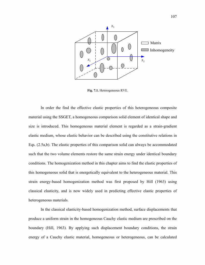
107

1x

3x

2x

Matrix

Inhomogeneity

Fig. 7.1. Heterogeneous RVE.

In order the find the effective elastic properties of this heterogeneous composite

material using the SSGET, a homogeneous comparison solid element of identical shape and

size is introduced. This homogeneous material element is regarded as a strain-gradient

elastic medium, whose elastic behavior can be described using the constitutive relations in

Eqs. (2.5a,b). The elastic properties of this comparison solid can always be accommodated

such that the two volume elements restore the same strain energy under identical boundary

conditions. The homogenization method in this chapter aims to find the elastic properties of

this homogeneous solid that is energetically equivalent to the heterogeneous material. This

strain energy-based homogenization method was first proposed by Hill (1963) using

classical elasticity, and is now widely used in predicting effective elastic properties of

heterogeneous materials.

In the classical elasticity-based homogenization method, surface displacements that

produce a uniform strain in the homogeneous Cauchy elastic medium are prescribed on the

boundary (Hill, 1963). By applying such displacement boundary conditions, the strain

energy of a Cauchy elastic material, homogeneous or heterogeneous, can be calculated

108

from the averaged stress and averaged strain. This uniform-strain boundary condition is

based on the assumption that the fluctuation wavelength of the applied strain is much larger

than the size of the RVE. That is, the applied strain to the RVE is macroscopically uniform.

However, when a material experiences a larger deformation gradient such that the mean

fields vary with the position of the RVE in the material, non-uniform strain boundary

conditions have to be applied to account for the strain gradient. One of such boundary

conditions is that the displacement on the boundary is approximated by the following

quadratic expression (e.g., Forest, 1998; Bigoni and Drugan, 2007):

0 0ˆ ( ) ( )i ij j ijk j ku x x x x x , (7.1)

where 0ij and 0

ijk are, respectively, the components of a second-order tensor and a third-

order tensor, xi is the ith component of the position vector x, and is the boundary of the

domain occupied by the RVE. Clearly, Eq. (7.1) shows that 00ikjijk . If 0

ijk = 0, Eq.

(7.1) recoveres the uniform-strain boundary condition used in Hill’s homogenization

method (Hill, 1963). The displacement in Eq. (7.1) must satisfy the Navier-like

displacement equilibrium equations give in Eq. (2.9) without body forces. Using Eq. (7.1)

in Eq. (2.9) together with 0jf , results in

0 0(2 1)iik kiiv , (7.2)

which gives three constraints on specifying 0ijk .

Substituting Eq. (7.1) into Eqs. (2.5c,d) yields the strain and strain gradient on the

boundary as

0 0 0 0 0ˆ ˆ( ) ( ) , ( )ij ij ijp jip p ijk ijk jikx x x (7.3a,b)

109

for any x . From Eqs. (7.3a,b), it is seen that the strain ij is linearly dependent on the

position x, while the strain gradient ijk is uniform on the boundary of the RVE. For a

homogeneous material subject to the boundary condition in Eqs. (7.3a,b), it is conceivable

that the strain gradient will be uniform throughout the material. This indicates that the

displacement throughout the material takes the same form as that given in Eq. (7.1), subject

to the constraints listed in Eq. (7.2). In other words, for a homogeneous material Eqs. (7.1)

and (7.3a,b) also hold for the interior points (i.e., x ).

However, if a heterogeneous material model is subject to the boundary condition

given in Eq. (7.1), the strain gradient in the interior will not be uniform as shown in Eq.

(7.3b) due to the disturbance of existing inhomogeneities. In general, for a heterogeneous

material, the strain and stress fields depend on the morphology and properties of the

constituents and their distributions in the material.

The volume-averaged strain energy, U, stored in a material based on the SSGET can

be expressed in terms of quantities on the boundary as (see Appendix I)

1 1( ) ( )

2Vol( ) 2Vol( )ij ij ijk ijk ij i j ijk ij kU dV u n n dA

, (7.4)

where n = niei is the outward unit normal vector on , ijk is the component of the strain

gradient tensor defined in Eq. (2.5d), and ijk is the component of the double stress tensor

defined in Eq. (2.5b). Using Eqs. (7.1) and (7.3a) in Eq. (7.4) gives

0 0 0 0 01( ) .

2Vol( ) ij im m j ijk ij k ij imn m n j ijk ijp jip p kU x n n x x n x n dA (7.5)

Applying the divergence theorem and the equilibrium equations 0, jij in Eq. (7.5) yields

dVxdVU ijppijijpijij )()(Vol

1

)(Vol2

1 00

. (7.6)

110

Eq. (7.6) gives the strain energy in an equilibrated material subject to the uniform strain

gradient boundary condition listed in Eq. (7.1). Note that Eq. (7.4)–(7.6) are valid for both

homogeneous and heterogeneous materials, for no assumption is made on material

properties in reaching Eq. (7.4).

For a homogeneous material, using the constitutive equations in Eqs. (2.5a,b) and

Eqs. (7.3a,b), which are valid for x , into Eq. (7.6) leads to

pkpklmkijpHijlmplmijp

Hijlmklmkij

Hijlmlmij

HijlmH LxxCxCxCCU

200000000 22

1

, (7.7)

where HU is the volume-averaged strain energy in the homogenous material, HijlmC and

L are, respectively, the stiffness tensor and the material length scale parameter of the

homogeneous material, and

denotes the volume average over the domain .

On the other hand, for a heterogeneous material with (N+1) phases (with each phase

defined as a collection of inhomogeneities whose shape, size and elastic properties are

identical), the volume-averaged strain energy obtained in Eq. (7.6) can be further expressed

as

)(2

1 )(

0

0

0

)(0

nnnijppij

nN

nijp

N

nij

nijC xU

, (7.8)

where use has been made of

n

ffN

n

n

0

)( , (7.9)

in which f is a continuous quantity in the domain , n is a subdomain of occupied by

the nth phase, is the union of n with n ranging from 0 to N. In Eqs. (7.8) and (7.9) and

throughout this chapter, the matrix is designated as the phase with n = 0, nrepresents

the volume-averaged value over n , and )(n is the volume fraction of the nth phase.

111

Note that in reaching Eq. (7.8), it has been assumed that each constituent of the

heterogeneous material is a homogeneous strain-gradient medium whose constitutive

behavior can be described by Eqs. (2.5a,b). Using Eqs. (2.5a,b) in Eq. (7.8) yields

N

nklp

npkl

nijkl

nijp

N

nkl

nijkl

nijC

nnnLxCCU

0

2)()()(0

0

)()(0

2

1 , (7.10)

where )(nijklC and L(n) are, respectively, the stiffness tensor and the material length scale

parameter for the nth phase.

To get the effective elastic property of the heterogeneous material, the volume-

averaged strain energy in the homogeneous comparison solid element given in Eq. (7.7) and

that in the heterogeneous material element given in Eq. (7.10) should be identical, which

requires

.

2

1

22

1

1

2)()()(0

1

)()(0

200000000

N

nklp

npkl

nijkl

nijp

N

nkl

nijkl

nij

pkpklmkijpHijlmplmijp

Hijlmklmkij

Hijlmlmij

Hijlm

nnnLxCC

LxxCxCxCC

(7.11)

From Eq. (7.11) HijlmC and L , which are, respectively, the effective stiffness tensor and the

effective material length scale parameter of the heterogeneous material can be determined.

Note that HijlmC and L should be independent of the location of the RVE. Therefore, the

origin of the coordinate system can be placed at the centroid of the RVE for convenience.

This givespx = 0. Then, Eq. (7.11) becomes

.

2

1

22

1

1

2)()()(0

1

)()(0

20000

N

nklp

npkl

nijkl

nijp

N

nkl

nijkl

nij

pkpklmkijpHijlmlmij

Hijlm

nnnLxCC

LxxCC

(7.12)

Considering that 0ij and 0

ijp can be chosen independently, Eq. (7.12) gives two sets

112

of equations

,0

)()(0

N

nkl

nijkl

nlm

Hijlm

nCC (7.13)

N

nklp

npkl

nijkl

npkpklmk

Hijlm

nn

LxCLxxC0

2)()()(202 . (7.14)

From Eqs. (7.13) and (7.14), it is seen that once the relation between n

ε and 0ε , and the

relation between n

xε , n

κ and 0β are known, the effective stiffness tensor HijlmC and

the effective material length scale parameter L can be determined for given volume fraction,

stiffness tensor and material length scale parameter of each constituent of the composite. Eq.

(7.13) is the same as what is obtained from the classical homogenization method (e.g.,

Weng, 1984; Li and Wang, 2008), where only a uniform strain 0ε is applied on the

boundary and both the constituents of the heterogeneous material and its homogeneous

equivalent are treated as Cauchy media.

It is clear from Eq. (7.12) that if only the uniform-strain boundary condition is

prescribed, i.e., 0ijk = 0 in Eqs. (7.1) and (7.12), the terms involving 0

ijp on the both sides of

Eq. (7.12) will vanish. As a result, Eq. (7.12) will be reduced to Eq. (7.13). In this case, the

effective material length scale parameter L will not be involved. This implies that if the

overall behavior of the heterogeneous material is expected to be characterized by the

constitutive relations in the SSGET, the uniform strain gradient boundary condition in Eq.

(7.1) (at least) has to be applied. This will lead to the determination of the effective material

length scale parameter L from Eq. (7.14).

HijlmC and L can be readily obtained from Eqs. (7.13) and (7.14) if the exact elastic

strain and strain gradient fields in each phase are known. The exact solution for the elastic

fields in a heterogeneous RVE subject to the boundary condition in Eq. (7.1) may only be

113

derived using the SSGET for inhomogeneities of simple shapes such as spherical and

cylindrical ones. For inhomogeneities of complex shapes, numerical/approximate solutions

will have to be sought and implemented to computationally complete the homogenization

analysis.

In the next section, an analytical method is utilized to solve HijlmC from Eq. (7.13).

The volume-averaged strain in each phase will be determined analytically using the

Eshelby tensors obtained in Chapters III–V.

7.3. New Homogenization Method Based on the SSGET

To solve Eq. (7.13) subject to the boundary condition in Eq. (7.1), the concept of

averaged strain, which was first proposed by Mori and Tanaka (1973), is used. It can be

imagined that the volume-averaged strain over the matrix, 0

ε , is different from that over

the whole heterogeneous material due to the presence of inhomogeneities. For simplicity,

one inhomogeneity will be considered here. The volume-averaged strain over this

inhomogeneity further differs from that over the matrix by a perturbed value n

d

ε . That is,

nn

d

εεε

0. (7.15)

To determine the volume-averaged strain n

ε in Eq. (7.15), an inclusion problem

will be introduced, where a homogeneous body, , made of the same material as that of the

matrix, contains an inclusion which is of identical shape and size with those of the

inhomogeneity. The inclusion is prescribed with a uniform stress-free eigenstrain *ε and

subject to the same averaged strain as in Eq. (7.15). The volume-averaged stresses over the

inclusion and over the inhomogeneity can be made equivalent by suitably adjusting *ε . In

114

other words, the inclusion and the inhomogeneity problems are equivalent in the sense that

their averaged strain and stress fields are identical. This equivalence states (Eshelby, 1957)

)(:)(:00

)(*)0(

nn

dnd

εεCεεεC , (7.16)

where )0(C and )(nC are, respectively, the fourth-order stiffness tensors of the matrix and the

inhomogeneity.

From the derivations in Chapter II (see Eq. (2.40)) and considering that the size of

the RVE is much larger than that of the inclusion, the volume-averaged disturbed strain due

to the uniform eigenstrain *ε over the domain occupied by an arbitrarily shaped 3-D

inclusion is

*: εSεnn

d

, (7.17)

wheren

S is the volume-averaged Eshelby tensor based on the SSGET over the inclusion

domain and has been obtain for spherical, cylindrical and elliptical inclusions in Chapters

III–V (see Eqs. (3.18), (4.29) and (5.33)).

Using Eq. (7.17) in Eq. (7.16), the eigenstrain can be obained as

0

:*

εQε , (7.18)

with

)(:]:)[( )0()(1)0()()0( CCCSCCQ

nn

n. (7.19)

Then from Eqs. (7.17)–(7.19) and (7.15), the volume-averaged strain over the inclusion

domain is related to that over the matrix through

0( : ) :

n n ε I S Q ε , (7.20)

where I is the fourth-order identity tensor. Using the following identity (Li and Wang,

115

2008):

(0) 1 ( ) (0) 1: :[ ] : ( )n n

n

I S Q I S C C C , (7.21)

Eq. (7.20) is found to be identical to what is obtained using the classical Mori-Tanaka

homogenization method based on classical elasticity (see Eqs. (7.16) and (7.17) in Qu and

Cherkaoui, 2006) except for the expression of .n

S n

S in Eq. (7.20) based on the

SSGET contains a material length scale parameter and hence can capture the inclusion size

effect, unlike its counterpart based on classical elasticity.

The above analysis involving a single inhomogeneity phase, which is a collection of

inhomogeneities with identical size, shape and elastic properties and hence having the

samen

S and Q, remains valid for other phases. Therefore, from Eq. (7.20), it follows

0:):()(

1

)0(

0

)(

εQSIIεεnn

nN

n

N

n

n , (7.22)

where the volume-averaged strain over the matrix domain is related to that over the whole

RVE.

Using Eqs. (2.5c) and (7.1) and 0

x gives

0εε

. (7.23)

Through Eqs. (7.20), (7.22) and (7.23) the relation between the applied strain, 0ε , on the

boundary of the RVE and the volume-averaged strain over the domain of each phase is

determined. Then, substituting Eqs. (7.23), (7.22) and (7.20) into (7.13) and letting the

coefficients of 0

ε on both sides of the equation be equal will result in

1

)(

1

)0()()(

1

)0()0( ):(:):(:

QSIIQSICCC

nn

nN

n

nnN

n

H (7.24)

116

as the effective stiffness tensor of the heterogeneous material. Note that the

inhomogeneities are assumed to be unidirectional. Therefore, the influence of the

inhomogeneity orientation distribution is not incorporated in Eq. (7.24).

From Eq. (7.24) it is seen that the effective stiffness tensor HC depends not only on

the shapes but also on the sizes of the inhomogeneities through the volume-averaged

Eshelby tensor, n

S , which involves the material length scale parameter of the matrix.

Therefore, this effective stiffness tensor based on the SSGET is expected to be able to

capture the experimentally observed particle size effect in composites (e.g., Kouzeli and

Mortensen, 2002; Vollenberg, and Heikens, 1989; Vollenberg, et al., 1989).

7.4. Numerical Results

Several examples are provided here to quantitatively illustrate the dependence of the

effective elastic properties of a heterogeneous material on inhomogeneity sizes, as

analytically demonstrated in the preceding section. For simplicity, a composite material

with two isotropic phases is chosen for analysis. For such a material, the total phase number

N = 2, and Eq. (7.24) becomes

1 1

(0) (1) 1[(1 ) : ( : )] :[(1 ) ( : )]H

C C C I S Q I I S Q , (7.25)

where )0(C and )1(C are, respectively, the fourth-order isotropic stiffness tensors of the

matrix and the inhomogeneity phase, is the volume fraction of the inhomogeneity phase,

and Q can be obtained from Eq. (7.19) with n = 1.

For a spherical inclusion with radius R, the volume-averaged Eshelby tensor

1S based on the SSGET given in Eq. (3.18) can be rewritten as

117

1

P SP SS S

S I I , (7.26)

where

,112

31

)1(15

108

,112

31

)1(3

1

)0(2

)0(2

2

)0(

2

)0(

3)0(

2

)0(

2

)0(

3)0(

L

R

L

R

eL

R

L

R

R

L

v

vS

eL

R

L

R

R

L

v

vS

S

P

(7.27)

and PI and SI are two fourth-order tensors whose components are, respectively, given by

klijjkiljlikPijklI

3

1

2

1 , klij

SijklI

3

1 . (7.28)

When the gradient effect is not considered (i.e., when L = 0), Eqs. (7.26) and (7.27) can be

reduced to the Eshelby tensor for a spherical inclusion based on classical elasticity:

1

C C P C SP SS S

S I I , (7.29a)

where

)1(15

108,

)1(3

1

v

vS

v

vS C

SCP

. (7.29b)

Using IP and IS given in Eq. (7.28), the stiffness tensors )0(C and )1(C can also be

decomposed as

(0) (0) (0)3 2P SK G C I I , (1) (1) (1)3 2P SK G C I I , (7.30)

where )0(K and )1(K are, respectively, the bulk moduli of the matrix and the inhomogeneity,

and )0(G and )1(G are, respectively, the shear moduli of the matrix and the inhomogeneity.

After using Eqs. (7.30) and (7.26) in Eq. (7.25), the effective stiffness tensor can be

obtained in the following closed form:

3 I 2 IH H P H SK G C , (7.31)

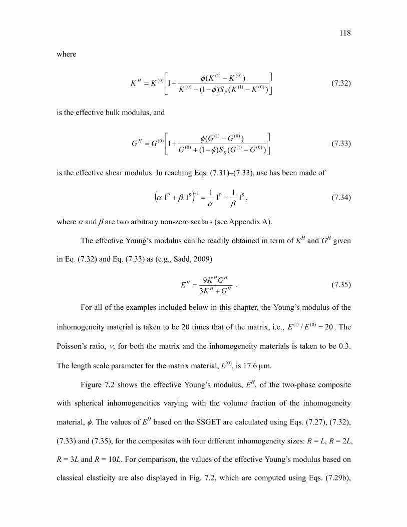
118

where

)()1(

)(1

)0()1()0(

)0()1()0(

KKSK

KKKK

P

H

(7.32)

is the effective bulk modulus, and

)()1(

)(1

)0()1()0(

)0()1()0(

GGSG

GGGG

S

H

(7.33)

is the effective shear modulus. In reaching Eqs. (7.31)–(7.33), use has been made of

SP1SP I1

I1

II

, (7.34)

where and are two arbitrary non-zero scalars (see Appendix A).

The effective Young’s modulus can be readily obtained in term of KH and GH given

in Eq. (7.32) and Eq. (7.33) as (e.g., Sadd, 2009)

HH

HHH

GK

GKE

3

9 . (7.35)

For all of the examples included below in this chapter, the Young’s modulus of the

inhomogeneity material is taken to be 20 times that of the matrix, i.e., 20/ )0()1( EE . The

Poisson’s ratio, , for both the matrix and the inhomogeneity materials is taken to be 0.3.

The length scale parameter for the matrix material, L(0), is 17.6 m.

Figure 7.2 shows the effective Young’s modulus, EH, of the two-phase composite

with spherical inhomogeneities varying with the volume fraction of the inhomogeneity

material, . The values of EH based on the SSGET are calculated using Eqs. (7.27), (7.32),

(7.33) and (7.35), for the composites with four different inhomogeneity sizes: R = L, R = 2L,

R = 3L and R = 10L. For comparison, the values of the effective Young’s modulus based on

classical elasticity are also displayed in Fig. 7.2, which are computed using Eqs. (7.29b),

119

(7.32) (7.33) and (7.35).

0

2

4

6

8

10

12

14

16

18

20

0 0.2 0.4 0.6 0.8 1

R = L

R = 2L

R = 3L

R = 10L

classical

R = L

R = 2L

R = 3L

R = 10L

Classical)0(E

E H

Fig. 7.2. Effective Young’s modulus of a composite with spherical inhomogeneities.

From Fig. 7.2, it is observed that EH based on the SSGET depends not only on the

volume fraction of the inhomogeneity phase, but also on the inhomogeneity size R. Also, it

is seen that the values of EH based on the SSGET are much larger than those based on

classical elasticity when R is small (with R = L = 17.6 m here). This agrees with the

experimental observations (Kouzeli and Mortensen, 2002): the smaller the inhomogeneity

size is, the stiffer the composite material is. As R increases, the curves for EH with the strain

gradient effect become closer to that (the dashed curve) based on classical elasticity, which

indicates that the strain gradient effect decreases as the inhomogeneity size increases. When

the inhomogeneity size R is much larger than L (e.g., R = 10L = 176 m here), the values of

EH approach the classical values, indicating that the strain gradient effect becomes

insignificant and therefore may be ignored. The same trend is observed for the effective

shear modulus of this composite containing spherical inhomogeneities.

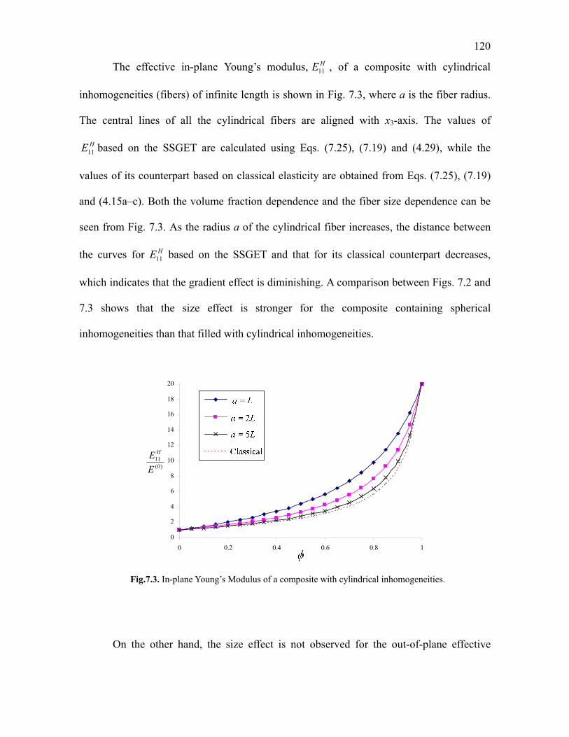
120

The effective in-plane Young’s modulus, HE11 , of a composite with cylindrical

inhomogeneities (fibers) of infinite length is shown in Fig. 7.3, where a is the fiber radius.

The central lines of all the cylindrical fibers are aligned with x3-axis. The values of

HE11 based on the SSGET are calculated using Eqs. (7.25), (7.19) and (4.29), while the

values of its counterpart based on classical elasticity are obtained from Eqs. (7.25), (7.19)

and (4.15a–c). Both the volume fraction dependence and the fiber size dependence can be

seen from Fig. 7.3. As the radius a of the cylindrical fiber increases, the distance between

the curves for HE11 based on the SSGET and that for its classical counterpart decreases,

which indicates that the gradient effect is diminishing. A comparison between Figs. 7.2 and

7.3 shows that the size effect is stronger for the composite containing spherical

inhomogeneities than that filled with cylindrical inhomogeneities.

0

2

4

6

8

10

12

14

16

18

20

0 0.2 0.4 0.6 0.8 1

R = L

R = 2L

R = 5L

classical

)0(11

E

E H

Fig.7.3. In-plane Young’s Modulus of a composite with cylindrical inhomogeneities.

On the other hand, the size effect is not observed for the out-of-plane effective

121

Young’s modulus HE33 for the composite with cylindrical inhomogeneities. Both HE33 based

on the SSGET and its counterpart base on classical elasticity are linearly dependent on the

volume fraction .

0

2

4

6

8

10

12

14

16

18

20

0 0.2 0.4 0.6 0.8 1

R = L

R = 2L

R = 5L

classical

a3 = L

a3 = 2L

a3 = 5L

Classical

)0(11

E

E H

Fig. 7.4. Effective HE11 of a composite with ellipsoidal inhomogeneities.

The effective Young’s moduli are displayed in Figs. 7.4 and 7.5 for composites

containing ellipsoidal inhomogeneities with three distinct semi-axes satisfying a1 : a2: a3 =

3 : 2 : 1. The a3-axis of each of the ellipsoidal inhomogeneities is aligned with the x3-axis in

the chosen Cartesian coordinate system. HE11 plotted in Fig. 7.4 is the effective Young’s

modulus in the x1-direction, while HE33 shown in Fig. 7.5 is the effective Young’s modulus

in the x3-direction. Both HE11 and HE33 are obtained from the orthotropic effective stiffness

tensor CH, calculated using Eqs. (7.25), (7.19) and (5.33). The size effect is clearly seen

from Figs. 7.4 and 7.5 for both HE11 and HE33 : the smaller a3 is, the larger the effective

Young’s modulus is. The size effect is more significant on HE33 than on HE11 , as indicated in

122

Figs. 7.4 and 7.5. This can be explained by the fact that the ellipsoidal inhomogeneities

have the smallest dimension along the x3-axis.

0

2

4

6

8

10

12

14

16

18

20

0 0.2 0.4 0.6 0.8 1

R = L

R = 2L

R = 5L

classical

)0(33

E

E H

Fig. 7.5. Effective HE33 of a composite with ellipsoidal inhomogeneities.

7.5. Summary

A homogenization method is developed in this chapter for predicting the effective

elastic properties of a heterogeneous material using the SSGET. The overall behavior of the

heterogeneous material is modeled as a homogeneous strain-gradient medium which is

characterized by the SSGET. The effective elastic properties of the heterogeneous material

are found to be dependent not only on the volume fractions, shapes and material properties

of the inhomogeneities but also on the inhomogeneity sizes, unlike what is predicted by the

homogenization methods based on classical elasticity. The effective elastic stiffness tensor

is analytically obtained by using the Mori-Tanaka and Eshelby’s equivalent inclusion

methods.

123

To quantitatively illustrate the effective elastic properties of the composite material,

sample numerical results are presented, which show that the inhomogeneity size has a

strong influence on the effective Young’s moduli when the inhomogeneity size is small (at

the micron scale). The composite becomes stiffer when the inhomogeneities become

smaller. It is also found that the inhomogeneity size effect on the effective Young’s moduli

becomes insignificant and may be neglected for composites filled by large inhomogeneities.

124

CHAPTER VIII

SUMMARY

The Eshelby inclusion problem of an inclusion embedded in an infinite homogeneous

isotropic elastic material and prescribed with an eigenstrain and an eigenstrain gradient is

solved analytically by using a simplified strain gradient elasticity theory (SSGET). This is

accomplished by first deriving the three-dimensional Green’s function in the SSGET in

terms of elementary functions using Fourier transforms. The fourth-order Eshelby tensor is

then obtained in a general form for an inclusion of arbitrary shape. The newly derived

Eshelby tensor consists of two parts: a classical part depending only on Poisson’s ratio, and

a gradient part depending on the length scale parameter additionally. The accompanying

fifth-order Eshelby-like tensor relating the prescribed eigenstrain gradient to the disturbed

strain is also obtained analytically. When the strain gradient effect is not considered, the

new Eshelby tensor reduces to that based on classical elasticity, and the Eshelby-like tensor

vanishes.

The expressions of the Eshelby tensor for the special cases of a spherical inclusion

and a cylindrical inclusion of infinite length are explicitly obtained by employing the

general form of the newly derived Eshelby tensor. The numerical results quantitatively

show that the components of the non-classical Eshelby tensor for either the spherical or the

cylindrical inclusion vary with both the position and the inclusion size, unlike their

counterparts in classical elasticity. For both the spherical and cylindrical inclusion problems,

it is found that when the inclusion radius is small the contribution of the gradient part is

significantly large and thus should not be ignored. For homogenization applications, the

volume average of the non-classical Eshelby tensor over the spherical inclusion or the

125

cylindrical inclusion is derived in a closed form. It is observed that the components of the

volume-averaged Eshelby tensor change with the inclusion size: the smaller the inclusion

radius is, the smaller the component values are. Also, the values of these components are

seen to approach from below those of their classical counterparts when the inclusion size

becomes sufficiently large.

Moreover, the more general and complex ellipsoidal inclusion problem is

analytically solved. By applying the general form of the Eshelby tensor in the SSGET, the

Eshelby tensor for an ellipsoidal inclusion is obtained in analytical expressions for both of

the regions inside and outside the inclusion in terms of two line integrals and two surface

integrals over a unit sphere. The Eshelby tensor for the ellipsoidal inclusion problem

includes those for the spherical and cylindrical inclusion problems based on the SSGET as

two limiting cases. The volume-averaged Eshelby tensor over the ellipsoidal inclusion is

also analytically obtained. Numerical results quantitatively show both the inclusion size

dependence and the position dependence exhibited by the components of the Eshelby tensor

derived. The same trend as that in the spherical and cylindrical inclusion problems is found

here: the smaller the ellipsoidal inclusion is, the smaller the values of the components of the

Eshelby tensor and its volume average are.

In order to incorporate the boundary effect, in addition to the particle size effect, a

solution for the Eshelby-type inclusion problem of a finite homogeneous isotropic elastic

body containing an inclusion is derived in a general form by using the SSGET. An extended

Betti’s reciprocal theorem and an extended Somigliana’s identity based on the SSGET are

proposed and utilized to solve the finite-domain inclusion problem. The solution for the

disturbed displacement field is expressed in terms of the Green’s function for an infinite

three-dimensional elastic body in the SSGET. It contains a volume integral term and a

126

surface integral term. The former is the same as that for the infinite-domain inclusion

problem based on the SSGET, while the latter represents the boundary effect. The solution

reduces to that of the infinite-domain inclusion problem when the boundary effect is not

considered. The problem of a spherical inclusion embedded concentrically in a finite

spherical elastic body is analytically solved by applying the general solution, with the

Eshelby tensor and its volume average obtained in closed forms. This Eshelby tensor

depends on the position, inclusion size, matrix size, and material length scale parameter and,

as a result, can capture the inclusion size and boundary effects, unlike existing ones. It

reduces to the Eshelby tensor based on classical elasticity for the spherical inclusion in an

infinite matrix if both the strain gradient and boundary effects are suppressed. Numerical

results reveal that the inclusion size effect can be quite large when the inclusion is very

small and that the boundary effect can dominate when the inclusion volume fraction is very

high. However, the inclusion size effect is diminishing as the inclusion becomes large

enough, and the boundary effect is vanishing as the inclusion volume fraction gets

sufficiently low.

Finally, a homogenization method based on the SSGET is developed to predict the

effective elastic properties of a heterogeneous (composite) material. The overall elastic

behavior of the heterogeneous material is characterized by a homogeneous elastic medium

that obeys the SSGET. An effective elastic stiffness tensor and an effective material length

scale parameter are obtained for the heterogeneous material by applying the Mori-Tanaka

and Eshelby’s equivalent inclusion methods. Numerical results show that both of them are

dependent not only on the volume fractions and shapes of the inhomogeneities but also on

the inhomogeneity sizes, unlike what is predicted by existing homogenization methods

based on classical elasticity. It is illustrated through numerical results for a two-phase

127

composite that the inhomogeneity size has a strong influence on the effective Young’s

moduli when the inhomogeneity size is small (at the micron scale). The composite becomes

stiffer when the inhomogeneities get smaller. However the inhomogeneity size effect on the

effective Young’s moduli becomes insignificant and may be neglected for a composite filled

with large inhomogeneities.

128

REFERENCES

Aifantis, E.C., 1999. Strain gradient interpretation of size effects. Int. J. Frac. 95,

299–314.

Aifantis, E.C., 2003. Update on a class of gradient theories. Mech. Mater. 35, 259–

280.

Altan, B.S., Aifantis, E.C., 1992. On the structure of the mode III crack-tip in

gradient elasticity. Scripta Met. 26, 319–324.

Altan, B.S., Aifantis, E.C., 1997. On some aspects in the special theory of gradient

elasticity. J. Mech. Behavior Mater. 8 (3), 231–282.

Arfken, G.B., Weber, H.-J., 2005. Mathematical Methods for Physicists, 6th ed.

Elsevier, San Diego.

Ashby, M.F., 1970. The deformation of plastically non-homogeneous materials. Phil.

Mag. 21, 399–424.

Bigoni, D., Drugan, W.J., 2007. Analytical derivation of Cosserat moduli via

homogenization of heterogeneous elastic materials. ASME J. Appl. Mech. 74, 741–753.

Cheng, Z.-Q., He, L.-H., 1995. Micropolar elastic fields due to a spherical inclusion.

Int. J. Eng. Sci. 33, 389–397.

Cheng, Z.-Q., He, L.-H., 1997. Micropolar elastic fields due to a circular cylindrical

inclusion. Int. J. Eng. Sci. 35, 659–668.

Eshelby, J.D., 1957. The determination of the elastic field of an ellipsoidal inclusion,

and related problems. Proc. R. Soc. Lond. A 241, 376–396.

Eshelby, J.D., 1959. The elastic field outside an ellipsoidal inclusion. Proc. R. Soc.

Lond. A 252, 561–569.

129

Evans, A.G., Hutchinson, J.W., 2009. A critical assessment of theories of strain

gradient plasticity. Acta Mater. 57, 1675–1688.

Fleck, N.A. , Hutchinson, J.W., 1997. Strain gradient plasticity. Adv. Appl. Mech.

33, 295–361.

Fleck, N.A., Muller, G.M., Ashby, M.F. , Hutchinson, J.W., 1994. Strain gradient

plasticity: theory and experiment. Acta Metall. Mater. 42, 475–487.

Forest, S., 1998. Mechanics of generalized continua: construction by

homogenization. J. Phys. IV France 8, 39–47.

Gao, H., Huang, Y., Nix, W.D., Hutchinson, J.W., 1999. Mechanism-based strain

gradient plasticity – I. Theory. J. Mech. Phys. Solids 47, 1239–1263.

Gao, X.-L., Ma, H. M., 2010a. Strain gradient solution for Eshelby’s ellipsoidal

inclusion problem. Proc. Royal Soc. A (published online in March 2010)

(doi:10.1098/rspa.2009.0631)

Gao, X.-L., Ma, H. M., 2010b. Solution of Eshelby's inclusion problem with a

bounded domain and Eshelby's tensor for a spherical inclusion in a finite spherical matrix

based on a simplified strain gradient elasticity theory. J. Mech. Phys. Solids (published

online in February 2010). (doi:10.1016/j.jmps.2010.01.006)

Gao, X.-L., Ma, H.M., 2009. Green’s function and Eshelby’s tensor based on a

simplified strain gradient elasticity theory. Acta Mech. 207, 163–181.

Gao, X.-L., Park, S.K., 2007. Variational formulation of a simplified strain gradient

elasticity theory and its application to a pressurized thick-walled cylinder problem. Int. J.

Solids Struct. 44, 7486–7499.

Gao, X.-L., 2008. Analytical solution for the stress field around a hard spherical

particle in a metal matrix composite incorporating size and finite volume effects. Math.

130

Mech. Solids 13, 357–372.

Gao, X.-L., Park, S. K., Ma, H.M., 2009. Analytical solution for a pressurized thick-

walled spherical shell based on a simplified strain gradient elasticity theory. Math. Mech.

Solids 14, 747–758.

Georgiadis, H.G., Vardoulakis, I., Velgaki, E.G., 2004. Dispersive Rayleigh-wave

propagation in microstructured solids characterized by dipolar gradient elasticity. J.

Elasticity 74, 17–45.

Giannakopoulos, A.E., Stamoulis, K., 2007. Structural analysis of gradient elastic

components. Int. J. Solids Struct. 44, 3440–3451.

Gourgiotis, P.A., Georgiadis, H.G., 2009. Plane-strain crack problems in

microstructured solids governed by dipolar gradient elasticity, J. Mech. Phys. Solids 57.

1898–1920.

Gradshteyn, I.S., Ryzhik, I.M., 2007. Table of Integrals, Series, and Products, Alan

Jeffrey and Daniel Zwillinger (Eds.), 7th ed. Academic Press, Boston.

Green, A.E., Rivlin, R.S., 1964a. Simple force and stress multipoles. Arch. Rat.

Mech. Anal. 16, 325–353.

Green, A.E., Rivlin, R.S., 1964b. Multipolar continuum mechanics. Arch. Rat. Mech.

Anal. 17, 113–147.

Hashin, Z., 1983. Analysis of composite materials—a survey. J. Appl. Mech. 50,

481–505.

Hill, R., 1963. Elastic properties of reinforced solids: some theoretical principles. J.

Mech. Phys. Solids 11, 357–372.

Ju, J. W., Sun, L. Z., 1999. A novel formulation for the exterior-point Eshelby's

tensor of an ellipsoidal inclusion. ASME J Appl. Mech. 66, 570–574.

131

Kakunai, S., Masaki, J., Kuroda, R., Iwata, K., Nagata, R., 1985. Measurement of

apparent Young’s modulus in the bending of cantilever beam by heterodyne holographic

interferometry. Exp. Mech. 25, 408–412.

Kinoshita, N., Mura, T., 1984. Eigenstrain problems in a finite elastic body. SIAM J.

Appl. Math. 44, 524–535.

Kiris, A., Inan, E., 2006. Eshelby tensors for a spherical inclusion in microstretch

elastic fields. Int. J. Solids Struct. 43, 4720–4738.

Koiter, W.T., 1964. Couple-stresses in the theory of elasticity: I and II. Proc. K. Ned.

Akad. Wet. B67 (1), 17–44.

Kouzeli, M., Mortensen, A., 2002. Size dependent strengthening in particle

reinforced aluminium. Acta Mater. 50, 39–51.

Kröner, E., 1963. On the physical reality of torque stresses in continuum mechanics.

Int. J. Eng. Sci. 1, 261–278.

Lakes, R., 1995. Experimental methods for study of Cosserat elastic solids and other

generalized elastic continua. In: Muhlhaus, H.(Ed.), Continuum Models for Materials with

Micro-Structure. Wiley, New-York, pp.1–22.

Lam, D.C.C., Yang, F., Chong, A.C.M., Wang, J., Tong, P., 2003. Experiments and

theory in strain gradient elasticity. J. Mech. Phys. Solids 51, 1477–1508.

Lazar, M., Maugin, G.A., 2005. Nonsingular stress and strain fields of dislocations

and disclinations in first strain gradient elasticity. Int. J. Eng. Sci. 43, 1157–1184.

Lazar, M., Maugin, G.A., Aifantis, E.C., 2005. On dislocations in a special class of

generalized elasticity. Phys. Stat. Sol. (b) 242, 2365–2390.

Lazopoulos, K.A., 2004. On the gradient strain elasticity theory of plates. Euro. J.

Mech. A/Solids 23, 843–852.

132

Li, S., Wang, G., 2008. Introduction to Micromechanics and Nanomechanics, World

Scientific, Singapore.

Li, S., Miskioglu, I., Altan, B.S., 2004. Solution to line loading of a semi-infinite

solid in gradient elasticity. Int. J. Solids Struct. 41, 3395–3410.

Li, S., Sauer, R.A., Wang, G., 2007. The Eshelby tensors in a finite spherical domain

– Part I: Theoretical formulations. ASME J. Appl. Mech. 74, 770–783.

Liu, L. P., 2008. Solutions to the Eshelby conjectures. Proc. Royal Soc. Lond. A 464,

573–594.

Lloyd, D.J., 1994. Particle reinforced aluminum and magnesium matrix composites.

Int. Mater. Rev. 39, 1–23.

Luo, H.A., Weng, G.J., 1987. On Eshelby's inclusion problem in a three-phase

spherically concentric solid, and a modification of Mori-Tanaka’s method. Mech. Mater. 6,

347–361.

Luo, H.A., Weng, G.J., 1989. On Eshelby's S-tensor in a three-phase cylindrically

concentric solid, and the elastic moduli of fiber-reinforced composites. Mech. Mater. 8, 77–

88.

Ma, H.M., Gao, X.-L., 2010. Eshelby’s tensors for plane strain and cylindrical

inclusions based on a simplified strain gradient elasticity theory. Acta Mech. 211, 115–129.

Ma, H.S., Hu, G.K., 2006. Eshelby tensors for an ellipsoidal inclusion in a

micropolar material. Int. J. Eng. Sci. 44, 595–605.

Ma, H.S., Hu, G.K., 2007. Eshelby tensors for an ellipsoidal inclusion in a

microstretch material. Int. J. Solids Struct. 44, 3049–3061.

Magnus, W., Oberhettinger, F., Soni, R.P., 1966. Formulas and Theorems for the

Special Functions of Mathematical Physics. Springer-Verlag, New York.

133

Maranganti, R., Sharma, P., 2007. A novel atomistic approach to determine strain-

gradient elasticity constants: Tabulation and comparison for various metals, semiconductors,

silica, polymers and the (Ir) relevance for nanotechnologies. J. Mech. Phy. Solids 55, 1823–

1852.

Markenscoff, X., 1998. Inclusions with constant eigenstress. J. Mech. Phys. Solids

46, 2297–2301.

Michelitsch, T.M., Gao, H., Levin, V.M., 2003. Dynamic Eshelby tensor and

potentials for ellipsoidal inclusions. Proc. R. Soc. Lond. A 459, 863–890.

Mindlin, R.D., Eshel, N.N., 1968. On first strain-gradient theories in linear elasticity.

Int. J. Solids Struct. 4, 109–124.

Mindlin, R.D., 1964. Micro-structure in linear elasticity. Arch. Rat. Mech. Anal. 16,

51–78.

Mindlin, R.D., 1965. Second gradient of strain and surface-tension in linear

elasticity. Int. J. Solids Struct. 1, 417–438.

Mori, T., Tanaka, K., 1973. Average stress in matrix and average elastic energy of

materials with misfitting inclusions. Acta Metall. 21, 571–574.

Mura, T., 1987. Micromechanics of Defects in Solids, 2nd ed. Martinus Nijhoff,

Dordrecht.

Nemat-Nasser, S., Hori, M., 1999. Micromechanics: Overall Properties of

Heterogeneous Materials, 2nd ed. Elsevier Science, Amsterdam, The Netherlands.

Nix, W.D., Gao, H., 1998. Indentation size effects in crystalline materials: a law for

strain gradient plasticity. J. Mech. Phys. Solids 46, 411–425.

Paris, F., Canas, J., 1997. Boundary Element Method: Fundamentals and

Applications. Oxford Science Publications, Oxford.

134

Polyzos, D., Tsepoura, K.G., Tsinopoulos, S.V., Beskos, D.E., 2003. A boundary

element method for solving 2-D and 3-D static gradient elastic problems Part I: Integral

formulation. Comput. Methods Appl. Mech. Engrg. 192, 2845–2873.

Qu, J., Cherkaoui, M., 2006. Fundamentals of Micromechanics of Solids. Wiley,

Hoboken, NJ.

Sadd, M.H., 2009. Elasticity: Theory, Applications, and Numerics, 2nd ed. Academic

Press, Burlington, MA.

Shi, M.X., Huang, Y., Hwang, K.C., 2000. Fracture in a higher-order elastic

continuum. J. Mech. Phys. Solids 48, 2513–2538.

Timoshenko, S.P., Goodier, J.N., 1970. Theory of Elasticity, 3rd ed. McGraw-Hill,

New York.

Toupin, R.A., 1962. Elastic materials with couple-stresses. Arch. Rat. Mech. Anal.

11, 385–414.

Vollenberg, P.H.T., Heikens, D., 1989. Particle size dependence of the Young’s

modulus of filled polymers: 1. Preliminary experiments. Polymer 30, 1656–1662.

Vollenberg, P.H.T., de Haan, J.W., van de Ven, L.J.M., Heikens, D., 1989. Particle

size dependence of the Young’s modulus of filled polymers: 2. Annealing and solid-state

nuclear magnetic resonance experiments. Polymer 30, 1663–1668.

Weng, G. J., 1984. Some elastic properties of reinforced solids, with special

reference to isotropic ones containing spherical inclusions. Int. J. Eng. Sci. 22, 845–856.

Xun, F., Hu, G.K., Huang, Z.P., 2004. Effective in plane moduli of composites with

a micropolar matrix and coated fibers. Int. J. Solids Struct. 41, 247–265.

Zhang, X., Sharma, P., 2005. Inclusions and inhomogeneities in strain gradient

elasticity with couple stresses and related problems. Int. J. Solids Struct. 42, 3833–3851.

135

Zheng, Q.-S., Zhao, Z.-H., 2004. Green’s function and Eshelby’s fields in couple-

stress elasticity. Int. J. Multiscale Comput. Eng. 2, 15–27.

136

APPENDIX A

Note that in reaching Eq. (2.13b) use has been made of the following identity:

,I1

I1

II1

Sij

Pij

Sij

Pij

(A.1)

where , are two arbitrary non-zero scalars, 00I jiSij are the components of a second-

order spin tensor 00 ξξI S (with 0ξ being a unit vector introduced in Eq. (2.12)),

00I jiijPij are the components of the associated projection tensor IP = I IS, with I =

ijeiej being the second-order identity tensor. Eq. (A.1) can be easily proved by using the

definition of an inverse matrix.

137

APPENDIX B

In this appendix, it is shown that the integration result given in Eq. (2.18) is true.

That is,

)cos31(sin 20022

0

00

jiijji xxd . (B.1)

[Proof] For the chosen spherical coordinate system (, , ) in the transformed space where

the position vector = 0ξ makes the angle with the position vector x (with the direction

of x being where = 0) in the physical space, one can write the unit vector in the

direction as

,)sinsincos(cos 0000 zyxξ (B.2)

where x0 is the unit vector along the x direction, and y0 and z0 are the unit vectors

perpendicular to x0. In component form, Eq. (B.2) reads

.)sinsincos(cos 0000 iiii zyx (B.3)

Then, it follows from Eq. (B.3) that

.sinsincossinsinsincossin

cossinsincossincoscossin

sincossincoscossincos

220020000

200220000

000020000

jijiji

jijiji

jijijiji

zzyzxz

zyyyxy

zxyxxx

(B.4)

Note that

.sin,cos,0cossin,0sin,0cos2

0

22

0

22

0

2

0

2

0

ddddd

(B.5)

Integrating on both sides of Eq. (B.4), together with the use of Eq. (B.5), results in

.sinsincos2 2002002002

0

00

jijijiji zzyyxxd (B.6)

138

Notice that

,

)]()()[(

)()()(

))(())(())((

000000

000000

000000000000

ijji

ji

jijiji

jijijijijiji zzyyxx

Iee

ezzyyxxe

ezzeeyyeexxe

ezezeyeyexex

(B.7)

where the fourth equality is based on the fact that the three orthogonal unit vectors x0, y0

and z0 form a set of base vectors in the 3-D physical space. Using Eq. (B.7) and the identity

sin2θ = 1 cos2θ in Eq. (B.6) will immediately give Eq. (B.1).

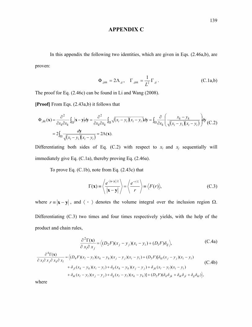
139

APPENDIX C

In this appendix the following two identities, which are given in Eqs. (2.46a,b), are

proven:

ijijkkijijkk L ,2,,, Γ1

Γ,Λ2Φ . (C.1a,b)

The proof for Eq. (2.46c) can be found in Li and Wang (2008).

[Proof] From Eqs. (2.43a,b) it follows that

).(Λ22

)(Φ

Ω

ΩΩ

2

Ω

2

,

xy

yyyyxx

iiii

iiii

kk

kiiii

kkkkkk

yxyx

d

dyxyx

yx

xdyxyx

xxd

xx (C.2)

Differentiating both sides of Eq. (C.2) with respect to xi and xj sequentially will

immediately give Eq. (C.1a), thereby proving Eq. (2.46a).

To prove Eq. (C.1b), note from Eq. (2.43c) that

,)()(Γ rFr

ee LrL

yxx

yx

(C.3)

where yx r , and denotes the volume integral over the inclusion region .

Differentiating (C.3) two times and four times respectively yields, with the help of the

product and chain rules,

,)())()((

)(Γ12

2

ijiijjji

δFDyxyxFDxx

x (C.4a)

,))(()])(())((

))(())(())((

))(()[())()()()((

)(Γ

2

34

4

klijjlikjkilkkllijjjllik

iilljkjjkkiliikkjl

iijjkliijjkklllkji

δδδδδδFDyxyxδyxyxδ

yxyxδyxyxδyxyxδ

yxyxδFDyxyxyxyxFDxxxx

x

(C.4b)

where

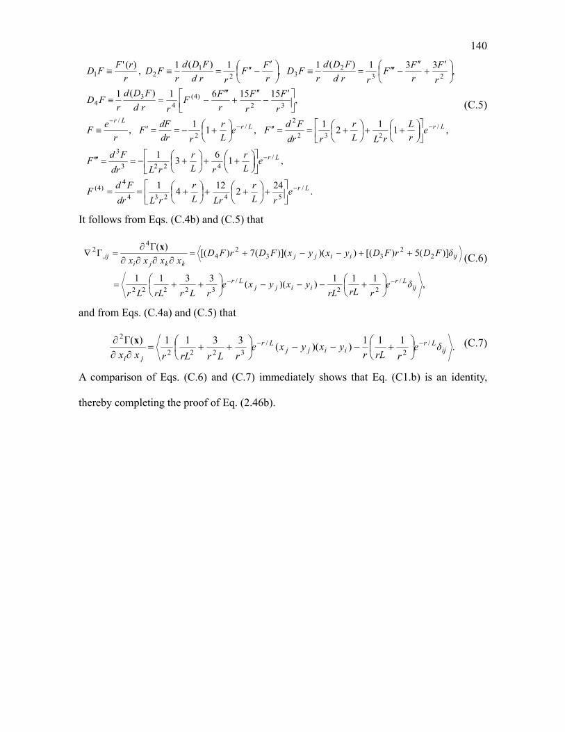
140

.24

212

41

,16

31

,11

21

,11

,

,151561

)(1

,331

)(1,

1

)(1,

)('

/54234

4)4(

/4223

3

/232

2/

2

/

32)4(

43

4

232

321

21

Lr

Lr

LrLrLr

erL

r

LrL

r

rLdr

FdF

eL

r

rL

r

rLdr

FdF

er

L

rLL

r

rdr

FdFe

L

r

rdr

dFF

r

eF

r

F

r

F

r

FF

rrd

FDd

rFD

r

F

r

FF

rrd

FDd

rFD

r

FF

rrd

FDd

rFD

r

rFFD

(C.5)

It follows from Eqs. (C.4b) and (C.5) that

,111

))((3311

)](5)[())()]((7)[(

)(ΓΓ

/22

/32222

22

332

4

4

,2

ijLr

iijjLr

ijiijjkkji

ij

δerrLrL

yxyxerLrrLLr

δFDrFDyxyxFDrFDxxxx

x(C.6)

and from Eqs. (C.4a) and (C.5) that

.111

))((3311

)(Γ /2

/3222

2

ijLr

iijjLr

ji

δerrLr

yxyxerLrrLrxx

x (C.7)

A comparison of Eqs. (C.6) and (C.7) immediately shows that Eq. (C1.b) is an identity,

thereby completing the proof of Eq. (2.46b).

141

APPENDIX D

For the infinitely long cylindrical inclusion of the radius a, which occupies the

domain , the scalar-valued function (x) defined in Eq. (2.43c) becomes, in the

cylindrical coordinate system (r, , y3) originated from the symmetry axis (as the y3-axis) of

the inclusion,

,)(

)(Γ2

0 3233

2

/)(

0

233

2

drddy

yxR

erx

LyxRa

(D.1)

where

.tan,,)()(1

212

2

2

1

2

22

2

11 y

yyyryxyxR (D.2a–c)

Note that

L

RKdt

tR

edy

yxR

e LtRLyxR

00 22

/

3233

2

/)(

22)(

22233

2

, (D.3)

where K0, as defined, is the modified Bessel function of the second kind of the zeroth order

(e.g., Gradshteyn and Ryzhik, 2007). Eq. (D.2a) can be rewritten as

cos222 rxrxR , (D.4)

where 2

2

2

1xxx x (as defined earlier) and α is the angle between the vectors x =

x1e1+x2e2 and R1 = y1e1+y2e2 on the plane y3 = 0. Clearly, α = θ − c, where c is the angle

between the specified vector x and the y1 axis and is a constant. Using the expression of R

given in Eq. (D.4) in K0( LR

) defined in Eq. (D.3) leads to (Magnus et al, 1966)

)()cos(2

)()cos(2

100

100

0

rxnL

xK

L

rI

L

xK

L

rI

rxnL

rK

L

xI

L

rK

L

xI

L

RK

nnn

nnn

(D.5a,b)

where In() and Kn() (n = 0, 1, 2, …) are the modified Bessel functions of the indicated

142

arguments.

Using Eqs. (D.3) and (D.5a,b) in Eq. (D.1) then gives, for any point x located inside

the inclusion (with x < a),

,4

44

4

)(cos2

)(cos22)(Γ

102

101001

0 0000

2

01

00

0

2

01

00

L

aK

L

xLaIL

L

aK

L

xLaI

L

xK

L

xI

L

xK

L

xILx

rdrL

rK

L

xIrdr

L

xK

L

rI

drrdcnL

rK

L

xI

L

rK

L

xI

drrdcnL

xK

L

rI

L

xK

L

rIx

x a

x

a

xn

nn

x

nnn

(D.6)

where use has been made of the following results:

),()]([),()]([,0)](cos[ 0101

2

0rrKrrK

drd

rIrrIrdrd

dcn

z

zKzIzKzI1

0110 . (D.7a–d)

Note that Eq. (D.7a) is a result of direct integration, whereas Eqs. (D.7b–d) are obtained

using the general formulas given in Magnus et al. (1966).

Similarly, substituting Eqs. (D.3) and (D.5b) into Eq. (D.1) yields, for any point x

located outside the inclusion (with x > a and thus r < a < x),

,44

)(cos22)(Γ

010 00

0

2

01

00

L

xK

L

aLaIrdr

L

xK

L

rI

drrdcnL

xK

L

rI

L

xK

L

rIx

a

a

nnn

(D.8)

where use has been made of Eqs. (D.7a,b). The final results obtained in Eqs. (D.6) and

(D.8) are exactly those listed in Eqs. (4.3a,b). They are also the same as those given in

Cheng and He (1997) for a similar scalar-valued function involved in their analysis based

143

on a micropolar elasticity theory. However, in this appendix the more general case with α =

θ – c (≠ θ) is considered and the derivation details are provided, which differ from what

was presented in Cheng and He (1997).

144

APPENDIX E

In this appendix, the expressions of (x) for the ellipsoidal inclusion problem given

in Eqs. (5.12) and (5.14) are derived.

Note that )(x in Eq. (2.43c) can be rewritten as

ΩΓ( )

r

Led

r

x y , (E.1)

where yx r . It can be shown using an inverse Fourier transform that

,e1

4Re

8

122

2

3

dξL

Lπ

πr

e iL

r

r (E.2)

where r (= x y) is the position vector of a point in the 3-D physical space, ξ is the position

vector of the same point in the Fourier (transformed) space Ω, i is the usual imaginary

number with i2 = −1. Using Eq. (E.2) in Eq. (E.1) then gives

,e1

1eRe

2)(

222

2

yx xy ddξLπ

L ii (E.3)

where is the region occupied by the ellipsoidal inclusion. Consider the coordinate

transformations:

,,

s

a

a

yY Ii

iI

ii (E.4)

where yi, Yi, i and i are, respectively, the components of y, Y, and , ,ξ and

2332

222

111

aξaξaξξ

s . (E.5)

Clearly, , as defined in Eq. (E.4), is a unit vector. Then, it follows from Eq. (E.4) that

145

.,,11: 321

2

3

3

2

2

2

2

1

1 YyYyY

sdaaad

a

y

a

y

a

y (E.6)

The use of Eq. (E.6) leads to

,)sin()cos(1

4

sine2e

33321

1

0 0

2cos321

ssss

aaa

dYYdaaad Yξsii

yyξ

(E.7)

where the inclination angle

in the chosen spherical coordinate system (Y,

, ) is

measured relative the direction of . Substituting Eq. (E.7) into Eq. (E.3) then yields

dLs

sssaaaL xx cos

1

)sin()cos(2)(

22333212

(E.8)

To evaluate the integral in Eq. (E.8), consider the following coordinate

transformations:

I

iiIii a

xXaK , , (E.9a,b)

where Ki and xi are, respectively, the components of K (with the magnitude K) and x (with

the magnitude x). Also, a convenient spherical coordinate system (K, , ) is chosen such

that the angle between K and X (with the magnitude X) is , with the direction of X being

the axis where = 0. As a result,

.cos,sinsin,cossin 321 KKKKKK (E.10)

Using Eqs. (E.9a,b) and (E.10) then gives

,cosXKxξ

, θsXξξ

mξsKKK ii

(E.11a,b)

),(cossinsincossin

2/12

3

2

2

2

1

s

aaas

, (E.11c)

where use has also been made of Eq. (E.5) in reaching Eq. (E.11a) and the fact that

146

ii to obtain Eq. (E.11c). Finally, it follows from Eqs. (E.9a), (E.10) and (E.11a) that

cos),(,sinsin),(,cossin),(3

32

21

1 sa

sa

sa

(E.12)

as the coordinate transformation from the Cartesian system (1, 2, 3) to the curvilinear

system (, , ). The Jacobian of this transformation can be readily obtained from Eq.

(E.12) as

,sin2

321

3

θξaaa

sJ (E.13)

which leads to the volume element relation:

dddaaa

sd sin2

321

3

. (E.14)

With the help of the coordinate transformation in (E.12) and the associated volume

element relation in (E.14), Eq. (E.8) becomes

2

0 0

2

2

0 0 0 22

2

sin2

sin1

)cos()sin()cos(2)(

ddFL

dddL

msssLx

(E.15a)

where m and s are defined in Eqs. (E.11b,c), and

).,()1(

)cos()sin(

)1(

)cos()cos(0 2222

Fd

L

ms

L

mssF

(E.15b)

Note that (e.g., Gradshteyn and Ryzhik, 2007)

;0,0for4)1(

)cos()cos( )(||0 2

baee

πξd

ξ

ξbξa baba (E.16a)

.0,2

)cosh(2

,0),sinh(2

)1(

)cos()sin(0 2

abπ

beπ

baaeπ

ξdξξ

ξbξa

a

b

(E.16b,c)

For the interior case with x , there is .1/// 23

23

22

22

21

21 axaxax This means

147

that XiXi < 1 (see Eq. (E.9b) or 1 XX , thereby giving 0 < m < s for 0 <cos <1 or 0 <

m < s for 1 <cos <0 according to Eq. (E.11b) for any x . It then follows from Eqs.

(E.16a,c) that for the interior case with both 0 < m < s (or 0 < </2) and 0 < m < s (or /2

< <) there is

.cosh122

L

me

L

sF L

s (E.17)

Using Eq. (E.17) in Eq. (E.15a) then results in

2

0 0

22 sinexp14)( ddL

me

L

sLL L

s

x (E.18)

for the interior case with x , where m = sXcos from Eq. (E.11b), and s = s(, ) is

given in Eq. (E.11c). This completes the derivation of Eq. (5.12).

For the exterior case with x , there is 1/// 23

23

22

22

21

21 axaxax or 1X ,

which makes the comparison between the values of m and s (satisfying m = sXcos given in

Eq. (E.11b)) more involved. In fact, the following four situations now need to be

considered separately.

(1) 0 < s < m or Xθ /1cos > 0 (see Eq. (E.11b)): Using Eqs. (E.16a,b) gives

.sinhcosh2

)1(

L

s

L

s

L

se

πF L

m

(E.19)

(2) 0 < m < s or Xθ /1cos0 (see Eq. (E.11b)): Applying Eqs. (E.16a,c) yields

,cosh122

)2(

L

me

L

sF L

s (E.20)

which is the same as F for the interior case given in Eq. (E.17).

(3) 0 < m < s or 0cos||/1 X (see Eq. (E.11b)): The use of Eqs. (E.16a,c) leads to

148