M. Wu: ENEE631 Digital Image Processing (Spring'09) More on Motion Analysis More on Motion Analysis Spring ’09 Instructor: Min Wu Electrical and Computer Engineering Department, University of Maryland, College Park bb.eng.umd.edu (select ENEE631 S’09) [email protected] ENEE631 Spring’09 ENEE631 Spring’09 Lecture 18 (4/8/2009) Lecture 18 (4/8/2009)

M. Wu: ENEE631 Digital Image Processing (Spring'09) More on Motion Analysis Spring ’09 Instructor: Min Wu Electrical and Computer Engineering Department,
Jan 03, 2016
Welcome message from author
This document is posted to help you gain knowledge. Please leave a comment to let me know what you think about it! Share it to your friends and learn new things together.
Transcript
M. Wu: ENEE631 Digital Image Processing (Spring'09)
More on Motion AnalysisMore on Motion Analysis
Spring ’09 Instructor: Min Wu
Electrical and Computer Engineering Department,
University of Maryland, College Park
bb.eng.umd.edu (select ENEE631 S’09) [email protected]
ENEE631 Spring’09ENEE631 Spring’09Lecture 18 (4/8/2009)Lecture 18 (4/8/2009)
M. Wu: ENEE631 Digital Image Processing (Spring'09) Lec18 – More on Motion Analysis [2]
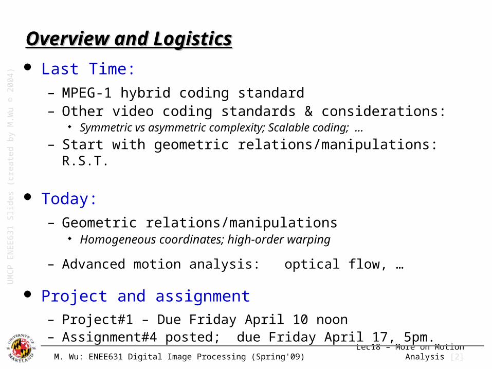
Overview and LogisticsOverview and Logistics Last Time:
– MPEG-1 hybrid coding standard– Other video coding standards & considerations:
Symmetric vs asymmetric complexity; Scalable coding; …
– Start with geometric relations/manipulations: R.S.T.
Today:
– Geometric relations/manipulations Homogeneous coordinates; high-order warping
– Advanced motion analysis: optical flow, …
Project and assignment– Project#1 – Due Friday April 10 noon– Assignment#4 posted; due Friday April 17, 5pm.
UM
CP
EN
EE
63
1 S
lide
s (c
rea
ted
by
M.W
u ©
20
04
)

M. Wu: ENEE631 Digital Image Processing (Spring'09) Lec18 – More on Motion Analysis [4]
Example of Example of Image RegistrationImage Registration
Figure from Gonzalez-Wood 3/e online book resource
M. Wu: ENEE631 Digital Image Processing (Spring'09) Lec18 – More on Motion Analysis [8]
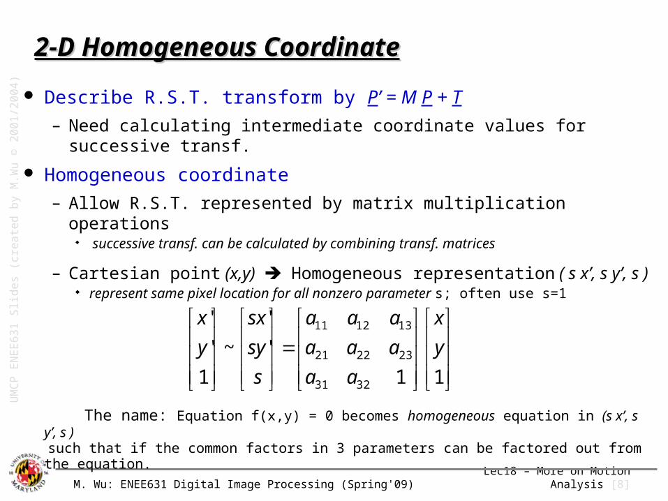
2-D Homogeneous Coordinate2-D Homogeneous Coordinate
Describe R.S.T. transform by P’ = M P + T
– Need calculating intermediate coordinate values for successive transf.
Homogeneous coordinate
– Allow R.S.T. represented by matrix multiplication operations successive transf. can be calculated by combining transf. matrices
– Cartesian point (x,y) Homogeneous representation ( s x’, s y’, s ) represent same pixel location for all nonzero parameter s; often
use s=1
The name: Equation f(x,y) = 0 becomes homogeneous equation in (s x’, s y’, s ) such that if the common factors in 3 parameters can be factored out from the equation.
1
1
'
'
~
1
'
'
3231
232221
131211
y
x
aa
aaa
aaa
s
sy
sx
y
x
UM
CP
EN
EE
63
1 S
lide
s (c
rea
ted
by
M.W
u ©
20
01
/20
04
)
M. Wu: ENEE631 Digital Image Processing (Spring'09) Lec18 – More on Motion Analysis [9]
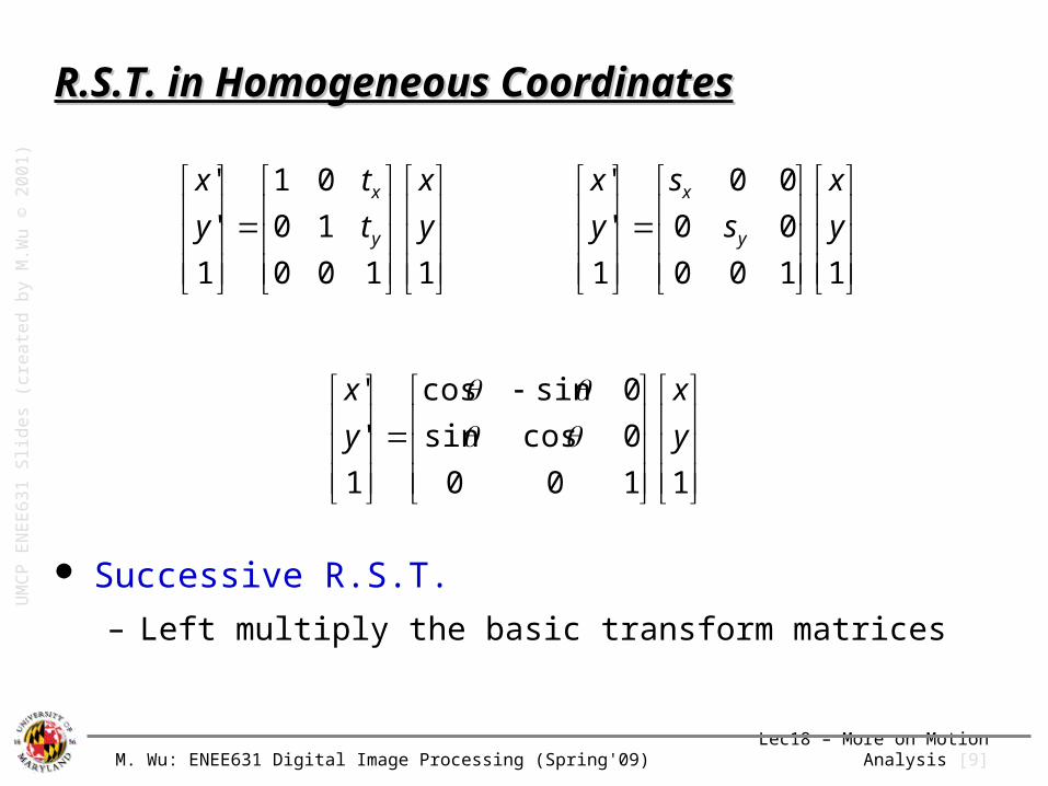
R.S.T. in Homogeneous CoordinatesR.S.T. in Homogeneous Coordinates
Successive R.S.T.
– Left multiply the basic transform matrices
1
100
10
01
1
'
'
y
x
t
t
y
x
y
x
1
100
00
00
1
'
'
y
x
s
s
y
x
y
x
1
100
0cossin
0sincos
1
'
'
y
x
y
x
UM
CP
EN
EE
63
1 S
lide
s (c
rea
ted
by
M.W
u ©
20
01
)
M. Wu: ENEE631 Digital Image Processing (Spring'09) Lec18 – More on Motion Analysis [10]
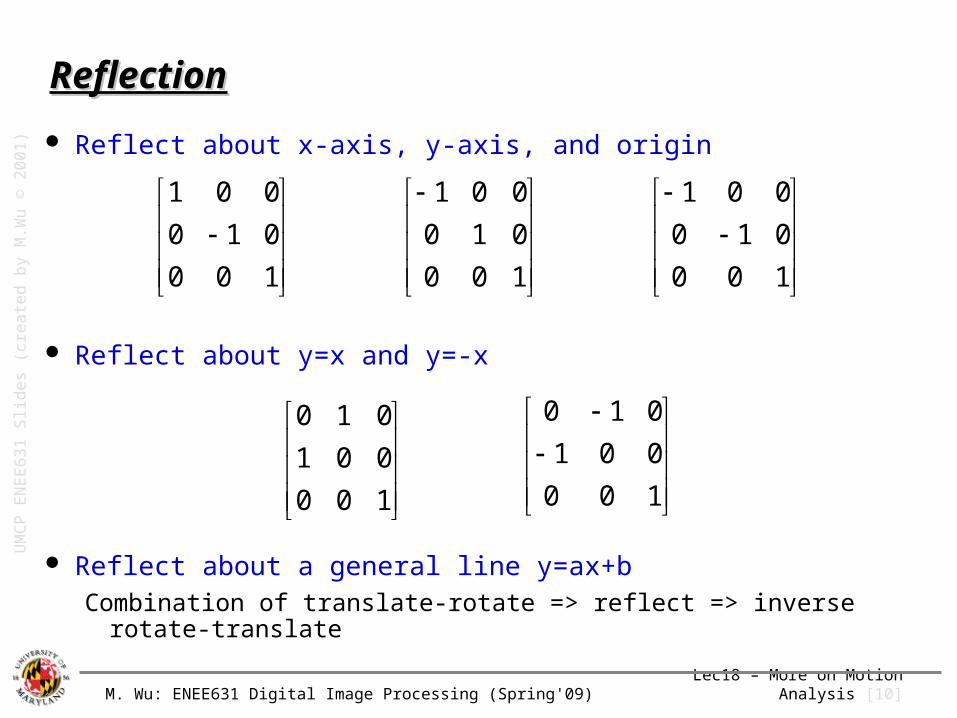
ReflectionReflection
Reflect about x-axis, y-axis, and origin
Reflect about y=x and y=-x
Reflect about a general line y=ax+bCombination of translate-rotate => reflect => inverse rotate-translate
100
010
001
100
010
001
100
010
001
100
001
010
100
001
010
UM
CP
EN
EE
63
1 S
lide
s (c
rea
ted
by
M.W
u ©
20
01
)
M. Wu: ENEE631 Digital Image Processing (Spring'09) Lec18 – More on Motion Analysis [11]
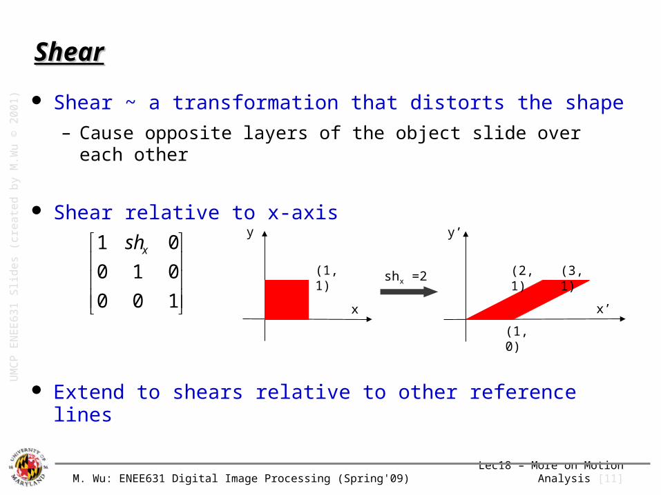
ShearShear
Shear ~ a transformation that distorts the shape
– Cause opposite layers of the object slide over each other
Shear relative to x-axis
Extend to shears relative to other reference lines
100
010
01
xsh(1, 1)
y
x
(1, 0)
y’
x’
(2, 1) (3, 1)shx =2
UM
CP
EN
EE
63
1 S
lide
s (c
rea
ted
by
M.W
u ©
20
01
)

M. Wu: ENEE631 Digital Image Processing (Spring'09) Lec18 – More on Motion Analysis [12]
General Composite TransformsGeneral Composite Transforms
Combined R.S.T. – {aij} is determined by
R.S.T. parameters
Rigid-body transform– Only involve translations and rotations– 2x2 rotation submatrix is orthogonal: row vectors are orthonormal
Extension to 3-D homogeneous coordinate– ( sX, sY, sZ, s ) with 4x4 transformation matrices
1
1001
'
'
232221
131211
y
x
aaa
aaa
y
x
UM
CP
EN
EE
63
1 S
lide
s (c
rea
ted
by
M.W
u ©
20
01
)

M. Wu: ENEE631 Digital Image Processing (Spring'09) Lec18 – More on Motion Analysis [14]
General Composite Transforms (cont’d)General Composite Transforms (cont’d) Affine transforms ~ 6 parameters
– Can be expressed as composition of RST,reflection and shear
– Parallel lines are transformed as parallel lines
Projective transforms ~ 8 parameters
– Cover more general geometric transformations between 2 planes Widely used in computer vision (e.g. image mosaicing, synthesized
views)
– Two unique phenomena: Chirping: increase in perceived spatial freq as distance to camera
increases Converging/Keystone effects: parallel lines appear closer & merging in
distance
1
1001
'
'
232221
131211
y
x
aaa
aaa
y
x
wc
bwAw y
x
cc
baa
baa
s
sy
sx
Tnew
yxw T
1
1
1
'
' ]','[
21
22221
11211
UM
CP
EN
EE
63
1 S
lide
s (c
rea
ted
by
M.W
u ©
20
01
)

M. Wu: ENEE631 Digital Image Processing (Spring'09) Lec18 – More on Motion Analysis [15]
Effects of Various Geometric MappingsEffects of Various Geometric Mappings
UM
CP
EN
EE
63
1 S
lide
s (c
rea
ted
by
M.W
u ©
20
04
)
From Wang’s Book Preprint Fig.5.18

M. Wu: ENEE631 Digital Image Processing (Spring'09) Lec18 – More on Motion Analysis [16]
Higher-order Nonlinear Spatial WarpingHigher-order Nonlinear Spatial Warping
Analogous to “rubber sheet stretching”
– Forward and reverse mapping of pixels’ coordinate indices
(x, y) (x’, y’)
Polynomial warping
– Extend affine transform to higher-order polynomial mapping– 2nd-order warping
x’ = a0 + a1 x + a2 y + a3 x2 + a4 xy + a5 y2
y’ = b0 + b1 x + b2 y + b3 x2 + b4 xy + b5 y2
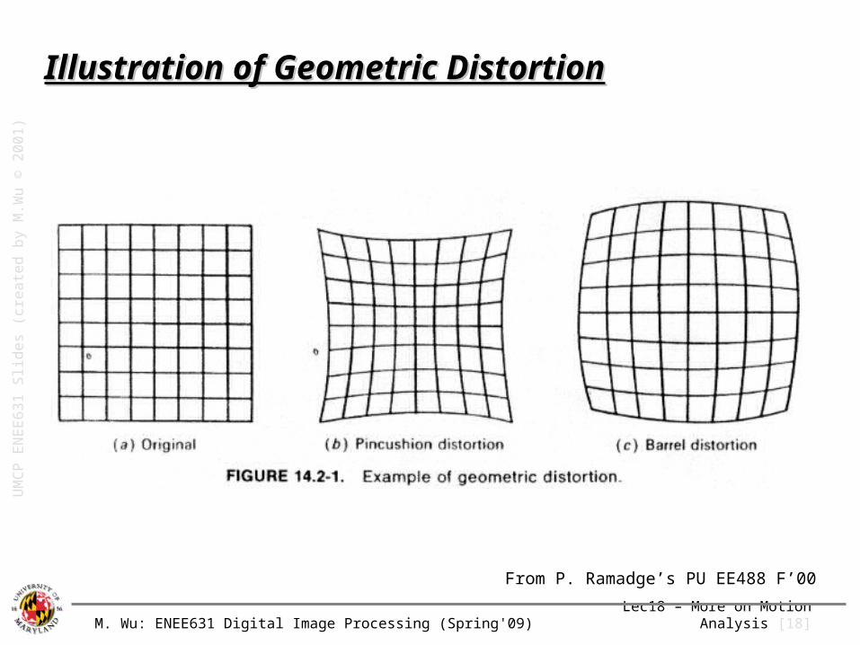
Spatial distortion in imaging system (lens)
– Pincushion and Barrel distortion
UM
CP
EN
EE
63
1 S
lide
s (c
rea
ted
by
M.W
u ©
20
01
)

M. Wu: ENEE631 Digital Image Processing (Spring'09) Lec18 – More on Motion Analysis [17]
Example of Example of 22ndnd-order -order Polynomial Polynomial Spatial Spatial WarpingWarping
UM
CP
EN
EE
63
1 S
lide
s (c
rea
ted
by
M.W
u ©
20
01
)
From P. Ramadge’s PU EE488 F’00
M. Wu: ENEE631 Digital Image Processing (Spring'09) Lec18 – More on Motion Analysis [18]
Illustration of Geometric DistortionIllustration of Geometric Distortion
UM
CP
EN
EE
63
1 S
lide
s (c
rea
ted
by
M.W
u ©
20
01
)
From P. Ramadge’s PU EE488 F’00
M. Wu: ENEE631 Digital Image Processing (Spring'09) Lec18 – More on Motion Analysis [19]
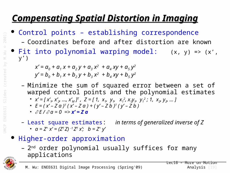
Compensating Spatial Distortion in ImagingCompensating Spatial Distortion in Imaging Control points – establishing correspondence
– Coordinates before and after distortion are known Fit into polynomial warping model: (x, y) => (x’, y’)
x’ = a0 + a1 x + a2 y + a3 x2 + a4 xy + a5 y2
y’ = b0 + b1 x + b2 y + b3 x2 + b4 xy + b5 y2
– Minimize the sum of squared error between a set of warped control points and the polynomial estimates
x’ = [ x’1, x’2, …, x’M ]T , Z = [ 1, x1, y1, x12, x1y1, y1
2 ; 1, x2, y2, … ]
E = ( x’ – Z a )T ( x’ – Z a ) + ( y’ – Z b )T ( y’ – Z b ) E / a = 0 => x’ = Z a
– Least square estimates: in terms of generalized inverse of Z a = Z^ x’ = (ZT Z) -1 ZT x’; b = Z^ y’
Higher-order approximation– 2nd order polynomial usually suffices for many applications
UM
CP
EN
EE
63
1 S
lide
s (c
rea
ted
by
M.W
u ©
20
01
)

M. Wu: ENEE631 Digital Image Processing (Spring'09) Lec18 – More on Motion Analysis [21]
Further Explorations on Motion EstimationsFurther Explorations on Motion Estimations
1. How to parameterize the underlying motion field?
2. What is the estimation criteria?
3. How to search for the optimal parameters?
UM
CP
EN
EE
63
1 S
lide
s (c
rea
ted
by
M.W
u ©
20
01
)
M. Wu: ENEE631 Digital Image Processing (Spring'09) Lec18 – More on Motion Analysis [22]
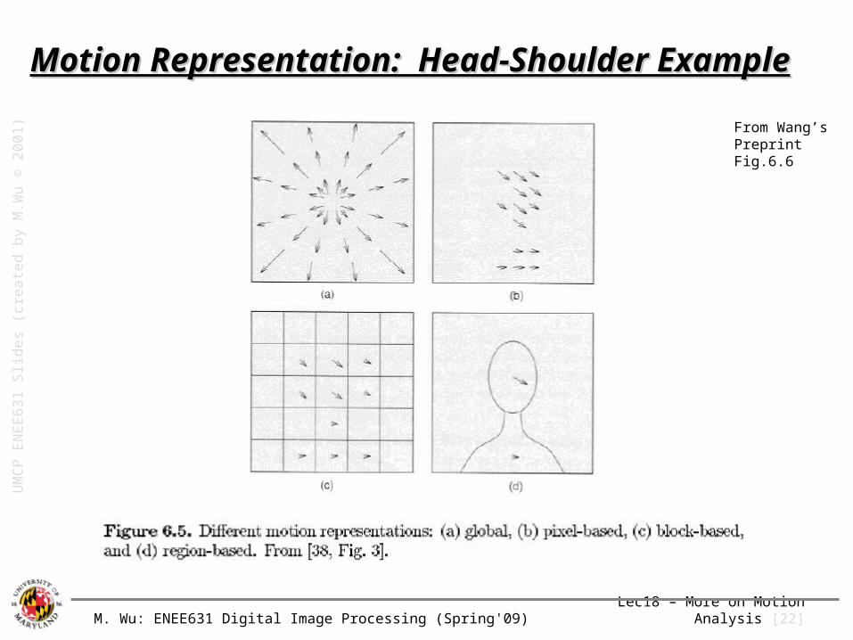
Motion Representation: Head-Shoulder ExampleMotion Representation: Head-Shoulder Example
From Wang’s Preprint Fig.6.6
UM
CP
EN
EE
63
1 S
lide
s (c
rea
ted
by
M.W
u ©
20
01
)
M. Wu: ENEE631 Digital Image Processing (Spring'09) Lec18 – More on Motion Analysis [23]
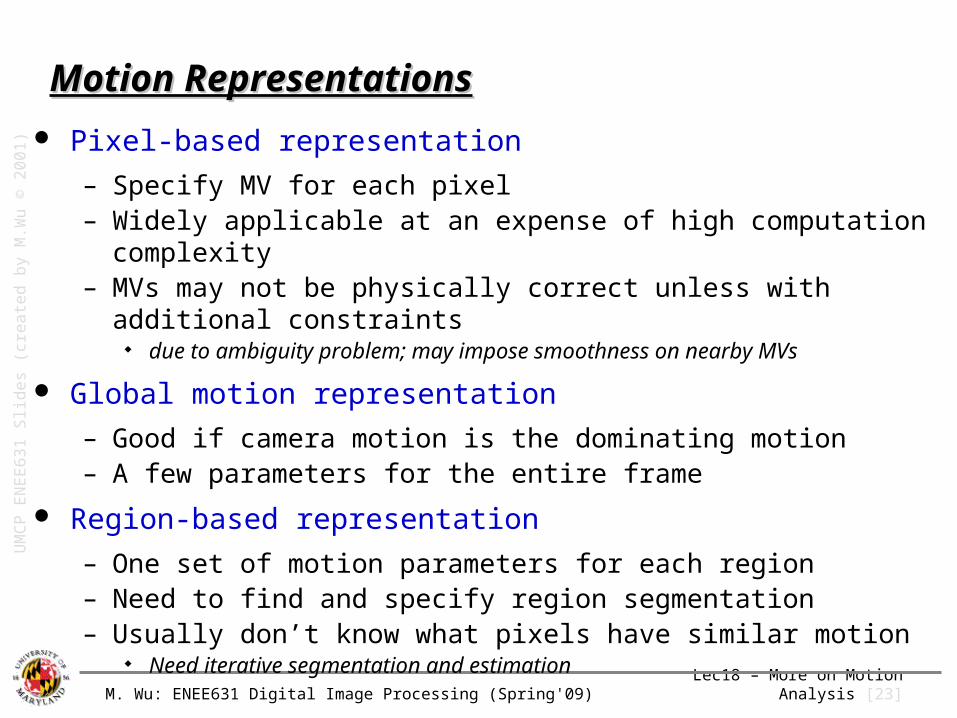
Motion RepresentationsMotion Representations
Pixel-based representation
– Specify MV for each pixel– Widely applicable at an expense of high computation complexity– MVs may not be physically correct unless with additional constraints
due to ambiguity problem; may impose smoothness on nearby MVs
Global motion representation
– Good if camera motion is the dominating motion– A few parameters for the entire frame
Region-based representation
– One set of motion parameters for each region– Need to find and specify region segmentation– Usually don’t know what pixels have similar motion
Need iterative segmentation and estimation
UM
CP
EN
EE
63
1 S
lide
s (c
rea
ted
by
M.W
u ©
20
01
)

M. Wu: ENEE631 Digital Image Processing (Spring'09) Lec18 – More on Motion Analysis [24]
Motion Representation (cont’d)Motion Representation (cont’d) Block-based representation
– Fixed partitioning into blocks and characterize each with simple model (e.g., translation model)
[Pro] Good compromise between accuracy and complexity, and shown success in video coding
[Con] False discontinuities of MVs between adjacent blocks
Mesh-based representation– Partition image into polygons and specify MV
for nodes– MVs of interior are interpolated from node MV
[Pro] Provide continuous motion everywhere; Good for facial and other non-rigid motions
[Con] Often fail to capture motion discontinuities at object boundaries
From R.Liu Seminar Course @ UMCP
UM
CP
EN
EE
63
1 S
lide
s (c
rea
ted
by
M.W
u ©
20
01
/20
04
)
M. Wu: ENEE631 Digital Image Processing (Spring'09) Lec18 – More on Motion Analysis [25]
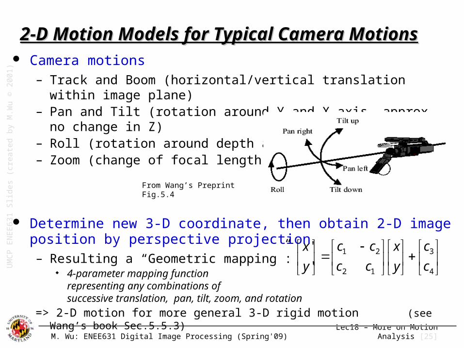
2-D Motion Models for Typical Camera Motions2-D Motion Models for Typical Camera Motions Camera motions
– Track and Boom (horizontal/vertical translation within image plane)– Pan and Tilt (rotation around Y and X axis, approx. no change in Z)– Roll (rotation around depth axis Z)– Zoom (change of focal length)
Determine new 3-D coordinate, then obtain 2-D image position by perspective projection– Resulting a “Geometric mapping”:
4-parameter mapping function representing any combinations of successive translation, pan, tilt, zoom, and rotation
=> 2-D motion for more general 3-D rigid motion (see Wang’s book Sec.5.5.3)
4
3
12
21
'
'
c
c
y
x
cc
cc
y
x
From Wang’s Preprint Fig.5.4
UM
CP
EN
EE
63
1 S
lide
s (c
rea
ted
by
M.W
u ©
20
01
)
M. Wu: ENEE631 Digital Image Processing (Spring'09) Lec18 – More on Motion Analysis [27]
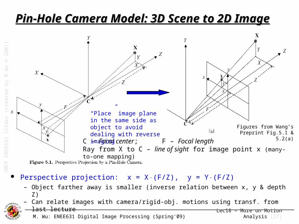
Pin-Hole Camera Model: 3D Scene to 2D ImagePin-Hole Camera Model: 3D Scene to 2D Image
Perspective projection: x = X(F/Z), y = Y(F/Z)– Object farther away is smaller (inverse relation between x, y & depth Z)– Can relate images with camera/rigid-obj. motions using transf. from last lecture
C – Focal center; F – Focal lengthRay from X to C – line of sight for image point x (many-to-one mapping)
“Place” image plane in the same side as object to avoid dealing with reverse imaging Figures from Wang’s
Preprint Fig.5.1 & 5.2(a)
UM
CP
EN
EE
63
1 S
lide
s (c
rea
ted
by
M.W
u ©
20
01
)

M. Wu: ENEE631 Digital Image Processing (Spring'09) Lec18 – More on Motion Analysis [28]
2-D Models Corresponding to 3-D Rigid Motion2-D Models Corresponding to 3-D Rigid Motion General case: six-parameter 3-D motion per object point
– Map to 2-D via perspective projection (scaling translation vector and object depth by same factor lead to same image)
– Mapping can change from point to point for arbitrary object surface
Projective transform– 8 parameters to relate any two planes in 3-D space– Either no translation along Z, or any motion of a planar object– Two unique phenomena: Chirping and converging/keystone effects
Chirping: equal-distance objects become closer as being farther away
Two parallel lines appear to move closer in distance
Approximation of projective mapping
– Affine motion (6 parameters): cannot capture converging & chirping– Bilinear motion (8 parameters): capture converging but not chirping
[Suggested readings: Wang’s book Sec. 5.5.3 & 5.5.4]
UM
CP
EN
EE
63
1 S
lide
s (c
rea
ted
by
M.W
u ©
20
04
)
M. Wu: ENEE631 Digital Image Processing (Spring'09) Lec18 – More on Motion Analysis [30]
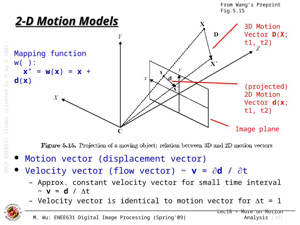
3D Motion Vector D(X; t1, t2)
(projected)2D Motion Vector d(x; t1, t2)
Image plane
Mapping function w( ): x’ = w(x) = x + d(x)
2-D Motion Models2-D Motion Models
Motion vector (displacement vector) Velocity vector (flow vector) ~ v = d / t
– Approx. constant velocity vector for small time interval ~ v = d / t– Velocity vector is identical to motion vector for t = 1
From Wang’s Preprint Fig.5.15U
MC
P E
NE
E6
31
Slid
es
(cre
ate
d b
y M
.Wu
© 2
00
1)

M. Wu: ENEE631 Digital Image Processing (Spring'09) Lec18 – More on Motion Analysis [31]
2-D Motion Field2-D Motion Field
Motion field
– {d ( x; t1, t2 )} for all image positions
Representing 2-D discrete motion fieldby vector graph
– Magnitude– Direction
From Wang’s Preprint Fig.5.16
UM
CP
EN
EE
63
1 S
lide
s (c
rea
ted
by
M.W
u ©
20
01
)
M. Wu: ENEE631 Digital Image Processing (Spring'09) Lec18 – More on Motion Analysis [32]
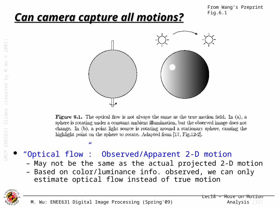
Can camera capture all motions?Can camera capture all motions?
“Optical flow”: Observed/Apparent 2-D motion– May not be the same as the actual projected 2-D motion– Based on color/luminance info. observed, we can only estimate
optical flow instead of true motion
From Wang’s Preprint Fig.6.1U
MC
P E
NE
E6
31
Slid
es
(cre
ate
d b
y M
.Wu
© 2
00
1)
M. Wu: ENEE631 Digital Image Processing (Spring'09) Lec18 – More on Motion Analysis [33]
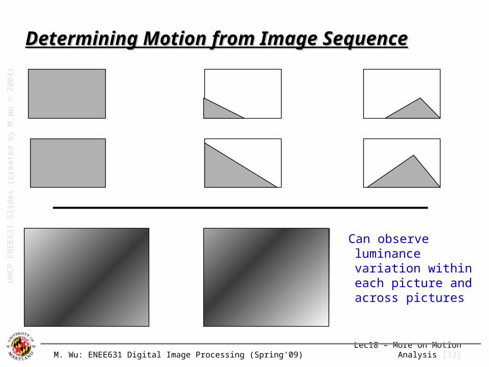
Determining Motion from Image SequenceDetermining Motion from Image Sequence
Can observe luminance variation within each picture and across pictures
UM
CP
EN
EE
63
1 S
lide
s (c
rea
ted
by
M.W
u ©
20
04
)
M. Wu: ENEE631 Digital Image Processing (Spring'09) Lec18 – More on Motion Analysis [34]
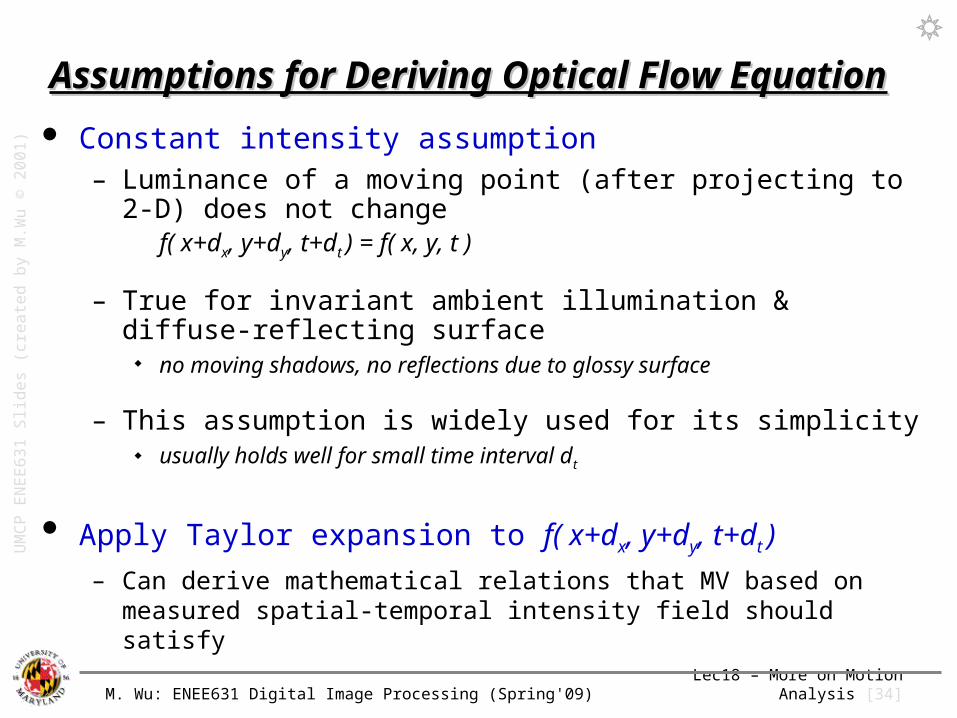
Assumptions for Deriving Optical Flow EquationAssumptions for Deriving Optical Flow Equation
Constant intensity assumption– Luminance of a moving point (after projecting to 2-D) does not
changef( x+dx, y+dy, t+dt ) = f( x, y, t )
– True for invariant ambient illumination & diffuse-reflecting surface no moving shadows, no reflections due to glossy surface
– This assumption is widely used for its simplicity usually holds well for small time interval dt
Apply Taylor expansion to f( x+dx, y+dy, t+dt ) – Can derive mathematical relations that MV based on measured spatial-
temporal intensity field should satisfy
UM
CP
EN
EE
63
1 S
lide
s (c
rea
ted
by
M.W
u ©
20
01
)

M. Wu: ENEE631 Digital Image Processing (Spring'09) Lec18 – More on Motion Analysis [35]
Optical Flow Equation (O.F.E.)Optical Flow Equation (O.F.E.)
tyx
tyx
dt
fd
y
fd
x
ftyxfLHS
tyxfdtdydxf
),,(
),,(),,( Const luminance assumpt.
1st order Taylor’s expansion
t)y,f(x, ofector gradient v spatial theis , here
0)(or , 0
0
T
yf
xf
Tyx
tyx
f
t
ff
t
fv
y
fv
x
f
dt
fd
y
fd
x
f
v
UM
CP
EN
EE
63
1 S
lide
s (c
rea
ted
by
M.W
u ©
20
01
/20
04
)
M. Wu: ENEE631 Digital Image Processing (Spring'09) Lec18 – More on Motion Analysis [36]
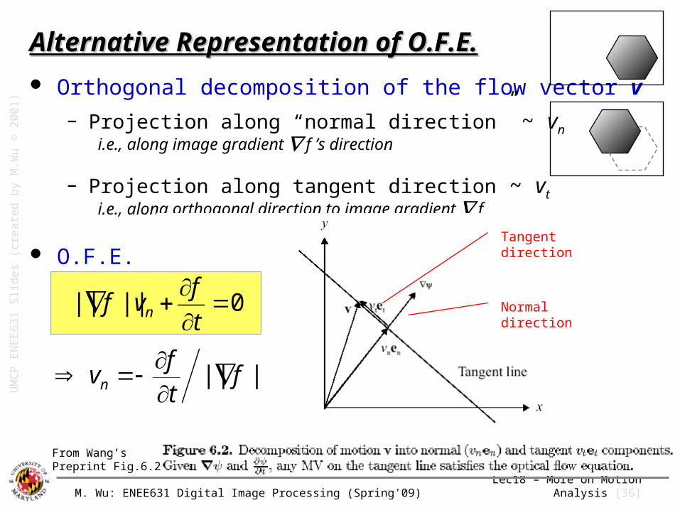
Alternative Representation of O.F.E.Alternative Representation of O.F.E.
Orthogonal decomposition of the flow vector v
– Projection along “normal direction” ~ vni.e., along image gradient f ’s direction
– Projection along tangent direction ~ vti.e., along orthogonal direction to image gradient f
O.F.E. f Normal direction
Tangent direction
0||||
t
fvf n
From Wang’s Preprint Fig.6.2
UM
CP
EN
EE
63
1 S
lide
s (c
rea
ted
by
M.W
u ©
20
01
)
|||| ftf
vn
M. Wu: ENEE631 Digital Image Processing (Spring'09) Lec18 – More on Motion Analysis [37]
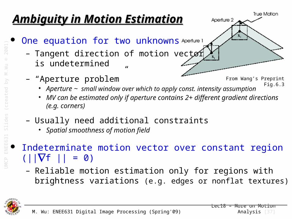
Ambiguity in Motion EstimationAmbiguity in Motion Estimation
One equation for two unknowns– Tangent direction of motion vector
is undetermined
– “Aperture problem” Aperture ~ small window over which to apply const. intensity
assumption MV can be estimated only if aperture contains 2+ different
gradient directions (e.g. corners)
– Usually need additional constraints Spatial smoothness of motion field
Indeterminate motion vector over constant region (||f || = 0)– Reliable motion estimation only for regions with brightness variations
(e.g. edges or nonflat textures)
From Wang’s Preprint Fig.6.3
UM
CP
EN
EE
63
1 S
lide
s (c
rea
ted
by
M.W
u ©
20
01
)

M. Wu: ENEE631 Digital Image Processing (Spring'09) Lec18 – More on Motion Analysis [39]
General Methodologies for Motion EstimationGeneral Methodologies for Motion Estimation
Two categories: Feature vs. Intensity based estimation
Feature based
– Step-1 establish correspondences between feature pairs – Step-2 estimate parameters of a chosen motion model by
least-square fitting of the correspondences
– Good for global/camera motion describable by parametric models Common models: affine, projective, … (Wang Sec.5.5.2-
5.5.4) Applications: Image mosaicing, synthesis of multiple-views
Intensity based
– Apply optical flow equation (or its variation) to local regions– Good for non-simple motion and multiple objects– Applications: video coding, motion prediction and filtering
UM
CP
EN
EE
63
1 S
lide
s (c
rea
ted
by
M.W
u ©
20
01
)

M. Wu: ENEE631 Digital Image Processing (Spring'09) Lec18 – More on Motion Analysis [40]
Summary of Today’s LectureSummary of Today’s Lecture
Advanced motion analysis– Capture 3-D scene and motion in 2-D camera plane– Relate two images for global motion analysis and image registration– Optical flow and optical flow equation for describing small motion– General approaches for estimating motion
Next Lecture: – Video content analysis
Readings
– Gonzalez’s 3/e book 2.6.5 (geometric transform)
– Wang’s book: Section 5.1, 5.3, 5.5, 5.6 (video modeling); 6.1 – 6.3 (motion analysis)

M. Wu: ENEE631 Digital Image Processing (Spring'09) Lec18 – More on Motion Analysis [41]
M. Wu: ENEE631 Digital Image Processing (Spring'09) Lec18 – More on Motion Analysis [43]
Key Issues for Motion EstimationKey Issues for Motion Estimation
1. How to parameterize the underlying motion field?
2. What is the estimation criteria?
3. How to search for the optimal parameters?
UM
CP
EN
EE
63
1 S
lide
s (c
rea
ted
by
M.W
u ©
20
01
)
M. Wu: ENEE631 Digital Image Processing (Spring'09) Lec18 – More on Motion Analysis [44]
Motion Estimation CriteriaMotion Estimation Criteria
Criterion based on displaced frame difference– E.g. in block matching approach
Criterion based on optical flow equations
Other criteria and considerations– Smoothness constraints– Bayesian criterion
UM
CP
EN
EE
63
1 S
lide
s (c
rea
ted
by
M.W
u ©
20
01
)

M. Wu: ENEE631 Digital Image Processing (Spring'09) Lec18 – More on Motion Analysis [45]
M.E. Criterion Based on Displaced Frame Diff.M.E. Criterion Based on Displaced Frame Diff.
Error of Displace Frame Difference (DFD)
Necessary condition for minimizing EDFD
– For p=2, Gradient of EDFD w.r.t. a is zero:
(MSE)Error SquaredMean ~2p
(MAD) Difference AbsoluteMean ~ 1p
parametersmotion of vector ~
framecurrent in set pixel the~
|)());((|
a
xaxwx
p
currefDFD ffE
0
a
DFDE
UM
CP
EN
EE
63
1 S
lide
s (c
rea
ted
by
M.W
u ©
20
01
)
M. Wu: ENEE631 Digital Image Processing (Spring'09) Lec18 – More on Motion Analysis [46]
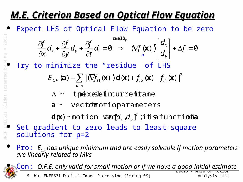
M.E. Criterion Based on Optical Flow EquationM.E. Criterion Based on Optical Flow Equation Expect LHS of Optical Flow Equation to be zero
Try to minimize the “residue” of LHS
Set gradient to zero leads to least-square solutions for p=2
Pro: EOF has unique minimum and are easily solvable if motion parameters are linearly related to MVs
Con: O.F.E. only valid for small motion or if we have a good initial estimate
axd
a
xxxdxax
offunction a isit ;],[tor motion vec ~)(
parametersmotion of vector ~
framecurrent in set pixel the~
|)()()())((|)( 121
Tyx
p
ttT
tOF
dd
fffE
0))((
0
small
fd
dfd
t
fd
y
fd
x
f
y
xTtd
tyx x
UM
CP
EN
EE
63
1 S
lide
s (c
rea
ted
by
M.W
u ©
20
01
)
M. Wu: ENEE631 Digital Image Processing (Spring'09) Lec18 – More on Motion Analysis [47]
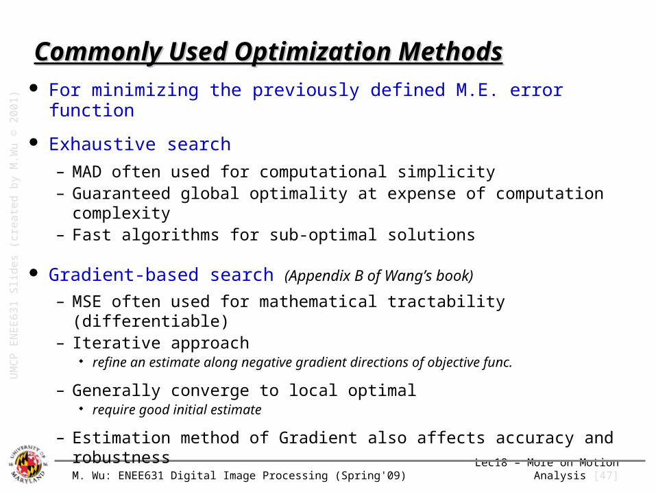
Commonly Used Optimization MethodsCommonly Used Optimization Methods For minimizing the previously defined M.E. error function
Exhaustive search
– MAD often used for computational simplicity– Guaranteed global optimality at expense of computation complexity– Fast algorithms for sub-optimal solutions
Gradient-based search (Appendix B of Wang’s book)
– MSE often used for mathematical tractability (differentiable)– Iterative approach
refine an estimate along negative gradient directions of objective func.
– Generally converge to local optimal require good initial estimate
– Estimation method of Gradient also affects accuracy and robustness
UM
CP
EN
EE
63
1 S
lide
s (c
rea
ted
by
M.W
u ©
20
01
)
M. Wu: ENEE631 Digital Image Processing (Spring'09) Lec18 – More on Motion Analysis [48]
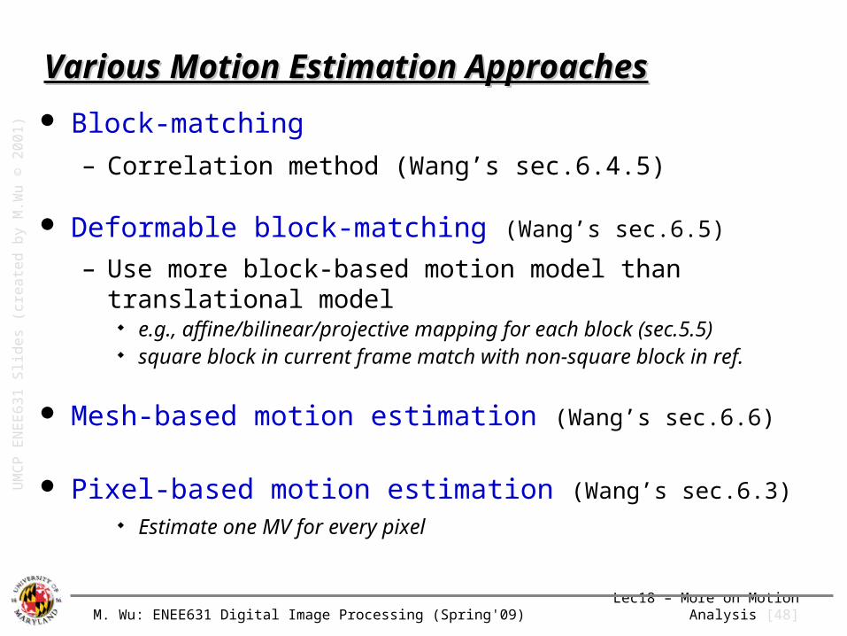
Various Motion Estimation ApproachesVarious Motion Estimation Approaches
Block-matching
– Correlation method (Wang’s sec.6.4.5)
Deformable block-matching (Wang’s sec.6.5)
– Use more block-based motion model than translational model e.g., affine/bilinear/projective mapping for each block
(sec.5.5) square block in current frame match with non-square block
in ref.
Mesh-based motion estimation (Wang’s sec.6.6)
Pixel-based motion estimation (Wang’s sec.6.3) Estimate one MV for every pixel
UM
CP
EN
EE
63
1 S
lide
s (c
rea
ted
by
M.W
u ©
20
01
)

M. Wu: ENEE631 Digital Image Processing (Spring'09) Lec18 – More on Motion Analysis [49]
Pixel-Based Motion EstimationPixel-Based Motion Estimation Estimate motion vectors at each pixel
– Based on Optical Flow Equation– Add smoothness constraints on motion field to avoid poor M.E. – Gradient based search ~ e.g., steepest gradient descent (Appendix B)
Motion estimation criterion– Expect LHS of O.F. Equation to be zero
– Try to minimize the “residue” of LHS
– Smoothness constraints Add magnitude of spatial gradient of velocity vectors to objective func.
0))((
0
small
fd
dfd
t
fd
y
fd
x
f
y
xTtd
tyx x
axd
a
xxxdxax
offunction a isit ;],[tor motion vec ~)(
parametersmotion of vector ~
framecurrent in set pixel the~
|)()()())((|)( 121
Tyx
p
ttT
tOF
dd
fffE
UM
CP
EN
EE
63
1 S
lide
s (c
rea
ted
by
M.W
u ©
20
01
)

M. Wu: ENEE631 Digital Image Processing (Spring'09) Lec18 – More on Motion Analysis [50]
Related Documents