Lyapunov Stability Analysis of a Competition Model with ...

Available online at https://ganitjournal.bdmathsociety.org/

GANIT: Journal of Bangladesh Mathematical Society

GANIT J. Bangladesh Math. Soc. 40.2 (2020) 95–110

DOI: https://doi.org/10.3329/ganit.v40i2.51311

Lyapunov Stability Analysis of a Competition Model with

Crowding Effects

Md. Kamrujjaman∗a, Kamrun Nahar Keyab, and Md Shafiqul Islam c

aDepartment of Mathematics, University of Dhaka, Dhaka 1000, BangladeshbDepartment of Science and Humanities, Military Institute of Science and Technology, Mirpur Cantonment, Dhaka 1216,

BangladeshcSchool of Mathematical and Computational Sciences, University of Prince Edward Island, Charlottetown, PE, Canada

ABSTRACT

The present study is connected to the analysis of a nonlinear system that covered a wide range of mathematicalbiology in terms of competition, cooperation, and symbiosis interactions between two species. We focus on howpopulations change their densities when two different species follow the non-symmetric logistic growth laws.We have investigated the stability of the corresponding densities of population, and to control the convergenceof solutions by proper choice of interacting constant and periodic parameters. It shows the effect of crowdingtolerance on both species. It will show that there exists an infinite number of coexistence solutions if theresource distributions are identical for both populations. If the carrying capacity of the first species exceeds therest one, then eventually the second population drops down to extinction. The results are presented studyingthe Lyapunov functional, phase portraits, and in a series of numerical examples.

c© 2020 Published by Bangladesh Mathematical Society

Received: July 27, 2020 Accepted: October 26, 2020 Published Online: January 15, 2021

Keywords: Lyapunov functional; stability; competition; crowding effects; phase portraits; numerical solutions.

AMS Subject Classifications 2020: 92D25, 35K57 (primary), 35K61, 37N25.

1 Introduction

The study of competition among different species is a prevailing feature in ecology. Different biological con-siderations are known to develop two-species competition models using different growth functions. Competitionarises whenever at least two species strive for a goal that cannot be shared, where one’s gain is the other’sloss. When they are only affected by their populations, then this type of competition is defined as intraspecificcompetition [1]. When resources are limited, several species may depend on these resources. Thus, each ofthe species competes with the others to gain access to the resources and this type of competition is known asinterspecific competition [2, 3, 4]. In interspecific competition species less suited to compete for the resourcesmay die out unless they adapt by character dislocation. In the literature, the well developed and most populargrowth laws were established in [5, 6, 7, 8, 9, 10]. In this paper, we develop a basic competition model based on

∗Corresponding author. E-mail address: [email protected]

96 Kamrujjaman et al. / GANIT J. Bangladesh Math. Soc. 40.2 (2020) 95–110

two different species either intraspecific or interspecific competition with two different growth rates and theircarrying capacities are non-identical. Taking into account of two different species, we consider the followingsystem of nonlinear differential equations with initial conditions:

dudt

= r1(t)u(t)

(1− u(t) + v(t)

k1(t)

), t > 0,

dvdt

= r2(t)u(t)

(1− u(t) + v(t)

k2(t)

), t > 0,

u(t0) = u0 > 0, v(t0) = v0 > 0.

(1.1)

This system of equations (1.1) consists of functions that are smooth and continuous. Here u and v denote thepopulation density of two species and k1, k2 represent their respective carrying capacity. Similarly, r1 and r2 arethe specific growth rates of u and v respectively. It is assumed that both functions defined in (1.1) are smoothenough, e.g., C1+α, 0 < α < 1 over time domain. The density of u and v is always positive since we assumethat population density is not negative. Henceforth (1.1) is an initial value problem with conditions u(t0) > 0and v(t0) > 0. Since the carrying capacity and growth rates of the two populations are distinct, the dynamicswill show the crowding effect behavior which is an important observation in the study. It is also remarked thatthe carrying capacities and intrinsic growth rates are time-periodic as well as constant. If carrying capacity ishigher in a habitat then the movement of the population will increase in the niche compared to other habitats;biologically the dynamics of the crowding effect will arise. We will discuss here how growth rates change dueto the change in carrying capacity and also give some illustrations on the stability of the population. Amongvarious methods for analyzing the stability of nonlinear systems, we use here a well-known method of Lyapunovfunctional.

Instead of logistic growth, let us consider the following function

f(t, u, k,M) = r(t)u(t)

(1− u(t)

k(t)

)(u(t)

M(t)− 1

), t > 0, (1.2)

where, r is the intrinsic growth rate, and k is the carrying capacity for population u. The function M is thesparse function and shows the Allee effect [11, 12, 13]. If 0 < M < k then there is a weak Allee effect while thestrong Allee effect is visible for M < 0 < k. If we consider the mathematical model introducing the functiondefined in (1.2), both crowding and Allee effect study can be observed. It is noted that the crowding out inecology is a result of competition by parasites within a host for finite resources. Typically, the severity of thiseffect increases with increasing numbers of parasites within a host and manifests in reduced body size and thusfitness. A strong Allee effect moves the species to extinction even for a weak Allee effect in many cases.

It is also noted that we introduced the linearization techniques [14] and linear differential equation theoryto analyze the steady states of our considered model. Often, mathematical models of real-world phenomenaare formulated in terms of systems of nonlinear differential equations [15, 16], which can be difficult to solveexplicitly. To overcome this barrier, we take a qualitative approach to the analysis of solutions to nonlinearsystems by making phase portraits and using stability analysis [17, 18, 19, 20]. We demonstrate these techniquesin the analysis of an individual problem in the area of nonlinear differential equations. The model is originallymotivated by population models in mathematical biology when solutions are required to be non-negative, butthe differential equations can be understood outside of this traditional scope of population models.

In mathematical modeling of ecology, the asymptotic behavior of the solutions of two species interactingpopulation has been central to understanding the coexistence and spatial dissociation of two species [21, 22,23]. In the weak competition case, the positive stationary solution (u, v) is globally asymptotically stableindependent of the diffusion coefficients. Materially, there exists a Lyapunov functional which allows for along-time asymptotic analysis [24]. The recent study has been proven that the directed dispersal organism hasevolutionary advantages to designing its own habitat for a competition coupled species model [25, 26].

We represent the stability of equilibria of the model in various parameters; at least two important constantsor periodic parameters that make the difference in the logistic growth model. It is found that if the competitionfavors the latter species, there is still a range of parameters for which there is coexistence. Numerical investiga-tion shows the long term behavior of the complete model that characterizes the population densities on severallevels. Throughout the entire study, we come to a conclusion of the stability of different competing species.

The rest of the paper is organized in the following way. In Section 2, we discuss the basic study of Lyapunovstability and Lyapunov functional. Section 3 presents the process of finding Lyapunov functional and techniquesof stability analysis through the Lyapunov function for a general system. In Section 4, we discuss the local

Kamrujjaman et al. / GANIT J. Bangladesh Math. Soc. 40.2 (2020) 95–110 97

and global stability of equilibriums with phase portrait. A number of examples are presented in Section 5 forapplications. Finally, Section 6 concludes the summary of the results and future discussions.

2 Preliminaries

In this section, we introduce some auxiliary results which are available in the literature [2, 7, 27, 28], andthese features will be used throughout the paper.

2.1 Lyapunov stability

Linear stability analysis tells us how a system behaves near an equilibrium point. It does not however tellus anything about what happens farther away from equilibrium. Phase-plane analysis combined with linearstability analysis can generally give us a full picture of the dynamics, but things become much more difficultin higher-dimensional spaces. In this section, we consider a technique due to Lyapunov which can be used todetermine the stability of an equilibrium point [10, 16, 29]. This method forms the basis of much of modernnonlinear control theory and also provides a theoretical justification for using local linear control techniques.Lyapunov stability is an intuitive approach to analyzing the stability and convergence of dynamic systemswithout explicitly computing the solutions of their differential equations.

To discuss Lyapunov stability for nonlinear equations we need to demonstrate some important definitionswhich are given below:

Definition 1. [27] A point x∗ is said to be an equilibrium point of

dx

dt= f(t, x) (2.1)

at time t0 if for all t ≥ t0, f(t, x∗) = 0.

Definition 2. [27] The equilibrium x = 0 of (2.1) is stable if, for each time t0, and for every constant R > 0,there exists some r(R, t0) such that

||x(t0)|| < r implies, ||x(t)|| < R for all t ≥ t0.

It is uniformly stable if r is independent of t0. The equilibrium is unstable if it is not stable.

Definition 3. [27] The equilibrium x = 0 of (2.1) is asymptotically stable if: (a) it is stable, and (b) for eachtime t0 there exists some r(t0) > 0 such that

||x(t0)|| < r ⇒ ||x(t)|| → 0 as t→∞

It is uniformly asymptotically stable if it is asymptotically stable and both r is independent of t0.

2.2 Lyapunov’s method

In many cases, it is possible to determine whether an equilibrium of a nonlinear system is locally stableby examining the stability of the linear approximation to the nonlinear dynamics about the equilibrium point.This approach is known as Lyapunov’s method.

Theorem 1. [27, 28] Let x = f(x), f(x∗) = 0 where x = dxdt and x∗ is in the interior of Ω ⊂ Rn. Assume that

V : Ω→ R is a function and

(i) V (x∗) = 0.

(ii) V (x) > 0 for all x ∈ Ω, x 6= x∗.


(iii) V (x) ≤ 0 along all trajectories of the system in Ω.

(iv) V < 0 for all x ∈ Ω, x 6= x∗.

If (i)-(iii) is satisfing then x∗ is said to be locally stable and if (iv) is also satisfied then x∗ is said to be locallyasymptotically stable.

A function that fulfills condition (i)-(iii) is called Lyapunov function.

2.3 Hartman-Grobman theorem

The Hartman-Grobman theorem is another important result in the local qualitative theory of ordinarydifferential equations (ODEs). The theorem shows that x = f(x) with f(0) = 0 and its linearized systemx = Df(x)x have the same qualitative structures near a hyperbolic equilibrium.

Definition 4. [27] Let A and B be subsets of Rn. A homomorphism A onto B is a continuous one-to-one mapH : A→ B such that H−1 : B → A. The two sets A and B are called homomorphic or topologically equivalent.Consider

x = f(x) (2.2)

Where x = 0 is a hyperbolic equilibrium. The linearized system

x = Ax (2.3)

where A = Df(0).

Theorem 2. [27] If x = 0 is a hyperbolic equilibrium (2.2) and (2.3), then there exists a homomorphism H ofan open set U containing the origin onto an open set V containing the origin such that for each x0 ∈ U , thereexists an open interval I0 ⊂ R containing the origin such that for all t ∈ I0

H φt(x0) = eAtH(x0)

3 Lyapunov Functional and Techniques of Stability Analysis

3.1 Construction of Lyapunov function

We can construct a Lyapunov function by two methods-one is a variable gradient method, and the otheris Krasovskii’s generalized method. In this paper, we grab the first method for analyzing the solution of theproposed model.

Assume that the gradient of the Lyapunov function V (x) is known up to some parameters.

∇V (x) = [V1, · · · · · · , Vn]T =

[∂V

∂x1, · · · · · · , ∂V

∂xn

]T

∇Vi =

n∑j=1

hijxj , i = 1, · · · · · · , n

Using the curl conditions ∂2V∂xi∂xj

= ∂∇Vi

∂xj=

∂∇Vj

∂xisimplify the coefficients hij for i, j = 1, · · · , n and hence

obtain V (x) ≡ ∂V∂x . Then integrate it to obtain V (x) as shown below

V (x) =

x∫0

∇V (x) dx

Executing this method, we have to keep in mind that the value of hij , i, j = 1, · · · , n should be chosen so that

V (x) is positive definite and V (x) is negative definite.


3.2 Techniques for solving nonlinear systems using eigenvalues

Consider a nonlinear system of differential equations using dummy variables x and y:x′ = f(x, y)

y′ = g(x, y)(3.1)

Where f and g are functions of two variables x = x(t) and y = y(t) such that f and g are not both linearfunctions of x and y. It is also noted that the notation x′ = dx

dt and y′ = dydt .

Unlike a linear system, a nonlinear system could have none, one, two, three, or any number of critical points.However, the critical points are found setting x′ = y′ = 0, and solve the resulting system

f(x, y) = 0

g(x, y) = 0

And every solution of this system of algebraic equations is an equilibrium point of the given system (3.1). Sincethere might be multiple equilibrium points present in the phase portrait, each trajectory could be influenced bymore than one equilibrium point. These results have a much more chaotic appearance of the phase portrait [29].We will approximate the behavior of the nearby trajectories using the linearizations of f and g. The techniqueconverts the nonlinear system into a linear system whose phase portrait approximates the local behavior of theoriginal nonlinear system near the equilibrium point.

Consider the Taylor series expansion about the equilibrium point (x, y) = (α, β) and we have

x′ = f(x, y) ≈ f(α, β) + fx(α, β)(x− α) + fy(α, β)(y − β)

y′ = g(x, y) ≈ g(α, β) + gx(α, β)(x− α) + gy(α, β)(y − β)

Since f(α, β) = 0 = g(α, β), the above linearizations become

x′ = f(x, y) = fx(α, β)(x− α) + fy(α, β)(y − β)

y′ = g(x, y) = gx(α, β)(x− α) + gy(α, β)(y − β)

Now it is a homogeneous linear system with a coefficient matrix

A =

(fx(α, β) fy(α, β)gx(α, β) gy(α, β)

)Above matrix is calculated by putting x = α, and y = β into the matrix of first partial derivatives

J(x, y) =

(fx fygx gy

)This matrix J(x, y) is often called the Jacobian matrix. It needs to be calculated once for each nonlinear system.For each critical point of the system, all we need to do is to compute the coefficient matrix of the linearizedsystem about the equilibrium point (x, y) = (α, β) and then use its eigenvalues to determine the stability.

4 Local and Global Stability Analysis

4.1 Linearization of the System

First, we have to linearize the system for further analysis. Rewrite the functions of equation (1.1) to findthe Lyapunov function as

r1(t)u(t)

(1− u(t) + v(t)

k1(t)

)= f(u, v)

r2(t)u(t)

(1− u(t) + v(t)

k2(t)

)= g(u, v)

(4.1)


To find the linearization matrices at the equilibria, we differentiate the equations of (4.1) and then obtain,

∂f

∂u=r1k1

(k1 − 2u− v)

∂f

∂v= − r1

k1u

∂g

∂u= − r2

k2v

∂g

∂v=r2k2

(k2 − u− 2v)

These partial functions produce the linearization matrix ∇V (u, v), and hence

∇V (u, v) =

∂f∂u

∂f∂v

∂g∂u

∂g∂v

( uv

)

and finally which yields

∇V (u, v) =

( r1k1

(k1 − 2u− v) − r1k1u

− r2k2v r2

k2(k2 − u− 2v)

)(uv

)(4.2)

Substituting the coordinates of the equilibrium points (0, 0), (k1, 0), (0, k2) and (u∗, v∗) into this formula, weobtain the linearization matrices to discuss the stability analysis of our main problem (1.1).

In the following section, we will consider all the equilibrium points to find stability or instability conditions.

4.2 Steady states analysis

Trivial equilibrium (0, 0): At the equilibrium point (u, v) = (0, 0), four partial derivatives are∂f∂u

= r1,

∂f∂v

= 0,∂g∂u

= 0,∂g∂v

= r2. Inserting these values in (4.2), we execute ∇(u, v):

∇V (u, v) =

(r1 00 r2

)(uv

)=

(r1ur2v

)Integrating the gradient function yields the Lyapunov function V such that

V (u, v) =

u∫0

r1x dx+

v∫0

r2y dy

= r1u2

2+ r2

v2

2> 0, r1 > 0, r2 > 0.

Let us now differentiate the previous function V (u, v), and we obtain

∂V

∂t= r1u

du

dt+ r2v

dv

dt

=r21k1u2(k1 − u− v) +

r22k2v2(k2 − u− v), using (1.1)

If ∂V∂t

> 0 by considering u > 0, v > 0 as Lyapunov stability conditions, it can be concluded that the equilibrium

point (0, 0) is locally unstable.


Due to the graphical analysis, the linearization matrix at (0, 0) is

A(0,0) =

(r1 00 r2

)(4.3)

We consider both r1 > r2 and r1 < r2. Let us first consider r1 = 2 and r2 = 1 which gives eigenvaluesλ1 = 2, λ2 = 1 and the corresponding eigenvectors(

10

)and

(01

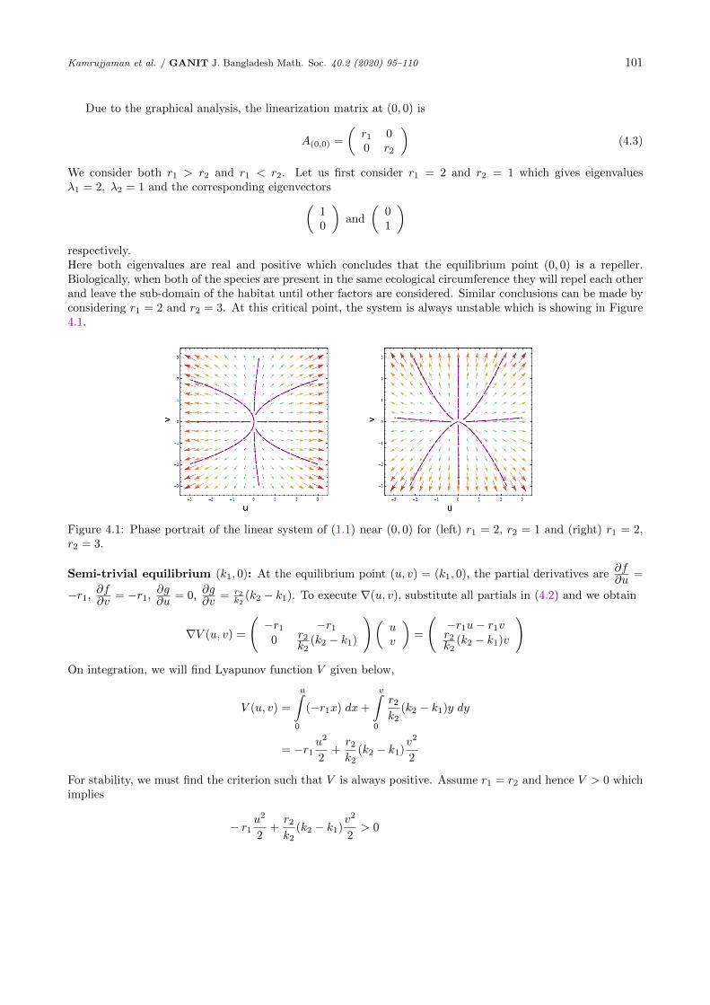
)respectively.Here both eigenvalues are real and positive which concludes that the equilibrium point (0, 0) is a repeller.Biologically, when both of the species are present in the same ecological circumference they will repel each otherand leave the sub-domain of the habitat until other factors are considered. Similar conclusions can be made byconsidering r1 = 2 and r2 = 3. At this critical point, the system is always unstable which is showing in Figure4.1.

Figure 4.1: Phase portrait of the linear system of (1.1) near (0, 0) for (left) r1 = 2, r2 = 1 and (right) r1 = 2,r2 = 3.

Semi-trivial equilibrium (k1, 0): At the equilibrium point (u, v) = (k1, 0), the partial derivatives are∂f∂u

=

−r1,∂f∂v

= −r1,∂g∂u

= 0,∂g∂v

= r2k2

(k2 − k1). To execute ∇(u, v), substitute all partials in (4.2) and we obtain

∇V (u, v) =

(−r1 −r1

0 r2k2

(k2 − k1)

)(uv

)=

(−r1u− r1vr2k2

(k2 − k1)v

)

On integration, we will find Lyapunov function V given below,

V (u, v) =

u∫0

(−r1x) dx+

v∫0

r2k2

(k2 − k1)y dy

= −r1u2

2+r2k2

(k2 − k1)v2

2

For stability, we must find the criterion such that V is always positive. Assume r1 = r2 and hence V > 0 whichimplies

− r1u2

2+r2k2

(k2 − k1)v2

2> 0


⇒ −u2k2 + (k2 − k1)v2 > 0, since r1 > 0, r2 > 0

⇒ (k2 − k1)

k2>u2

v2> 0.

which implies that k2 > k1. Now, differentiating the function V , we have

∂V

∂t= −r1u

du

dt+r2k2

(k2 − k1)vdv

dt

= − r21

k1u2(k1 − u− v) +

(r2k2

)2

(k2 − k1)v2(k2 − u− v)

For satisfying the Lyapunov condition, we must consider ∂V∂t

< 0. Hence either

− r21k1

(k1u2 − u3 − vu2) < 0

⇒ k1 > u+ v, r1 > 0, k1 > 0

Or (r2k2

)2

(k2 − k1)v2(k2 − u− v) < 0

⇒ 0 < k2 < u+ v if k2 > k1

However if k1 > k2 then we obtain the following inequalities

k2 > u+ v

Considering conditions, it can be clarified that for the case k1 > k2, the equilibrium point (k1, 0) is locally aswell as globally asymptotically stable independently of initial densities, see Figure 5.3(right).

Remark 1. It is noticed that both u > 0 and v > 0 throughout this section to satisfy all the inequalities ofstability analysis.

For the shake of graphical analysis, consider the linearization matrix at (k1, 0):

A(k1,0) =

(−r1 −r1

0 r2k2

(k2 − k1)

)(4.4)

where corresponding eigenvalues are λ1 = −r1 and λ2 = r2k2

(k2 − k1). Here λ2 > 0 if k2 > k1 and λ2 < 0 for

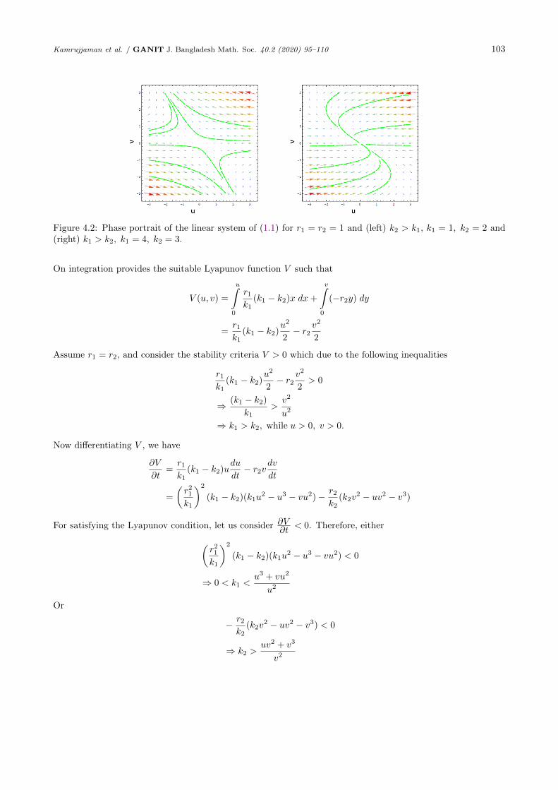
k2 < k1. Initially we consider r1 = r2 = 1 and k2 > k1, where k1 = 1, k2 = 2 and we obtain the eigenvaluesλ1 = −1 and λ2 = 0.5 and corresponding eigenvectors are(

10

)and

(−0.830770.556666

)respectively. Since both eigenvalues are negative, we can summarize the critical point (k1, 0) is an asymptoticallystable point shown in Figure 4.2 (right). So, in this case, as the species, v is extinct from the given ecologicalterritory, whereas the species u is the sole winner.Semi-trivial equilibrium (0, k2): At the equilibrium point (u, v) = (0, k2), the corresponding partial deriva-

tives are∂f∂u

= r1k1

(k1 − k2),∂f∂v

= 0,∂g∂u

= −r2,∂g∂v

= −r2. Substituting these values in (4.2), one can

implement ∇V (u, v) as:

∇V (u, v) =

(r1k1

(k1 − k2) 0

−r2 −r2

)(uv

)=

(r1k1

(k1 − k2)u

−r2u− r2v

)


Figure 4.2: Phase portrait of the linear system of (1.1) for r1 = r2 = 1 and (left) k2 > k1, k1 = 1, k2 = 2 and(right) k1 > k2, k1 = 4, k2 = 3.

On integration provides the suitable Lyapunov function V such that

V (u, v) =

u∫0

r1k1

(k1 − k2)x dx+

v∫0

(−r2y) dy

=r1k1

(k1 − k2)u2

2− r2

v2

2

Assume r1 = r2, and consider the stability criteria V > 0 which due to the following inequalities

r1k1

(k1 − k2)u2

2− r2

v2

2> 0

⇒ (k1 − k2)

k1>v2

u2

⇒ k1 > k2, while u > 0, v > 0.

Now differentiating V , we have

∂V

∂t=r1k1

(k1 − k2)udu

dt− r2v

dv

dt

=

(r21k1

)2

(k1 − k2)(k1u2 − u3 − vu2)− r2

k2(k2v

2 − uv2 − v3)

For satisfying the Lyapunov condition, let us consider ∂V∂t

< 0. Therefore, either(r21k1

)2

(k1 − k2)(k1u2 − u3 − vu2) < 0

⇒ 0 < k1 <u3 + vu2

u2

Or

− r2k2

(k2v2 − uv2 − v3) < 0

⇒ k2 >uv2 + v3

v2


Considering these two inequalities, we can conclude that if k2 > k1 then the equilibrium point (0, k2) is bothlocally and globally asymptotically stable for any non-negative and non-trivial initial values, see Figure 5.3(left).

To study the graphical analysis via phase plane, let us check the linearization matrix at (0, k2) such that

A(0,k2) =

(r1k1

(k1 − k2) 0

−r2 −r2

)(4.5)

where λ1 = r1/k1(k1 − k2) and λ2 = −r2 are respective eigenvalues. The eigenvalues λ1 > 0 if k1 > k2 andλ1 < 0 if k2 > k1. It is also seen that the eigenvalue λ2 is always negative. For instantaneous example, considerr1 = r2 and k1 > k2; specifically let us assume that k1 = 3, k2 = 2 and r1 = r2 = 1 and the respectiveeigenvalues are λ1 = −1 and λ2 = 0.33 with corresponding eigenvectors:(

01

)and

(0.799278−0.600961

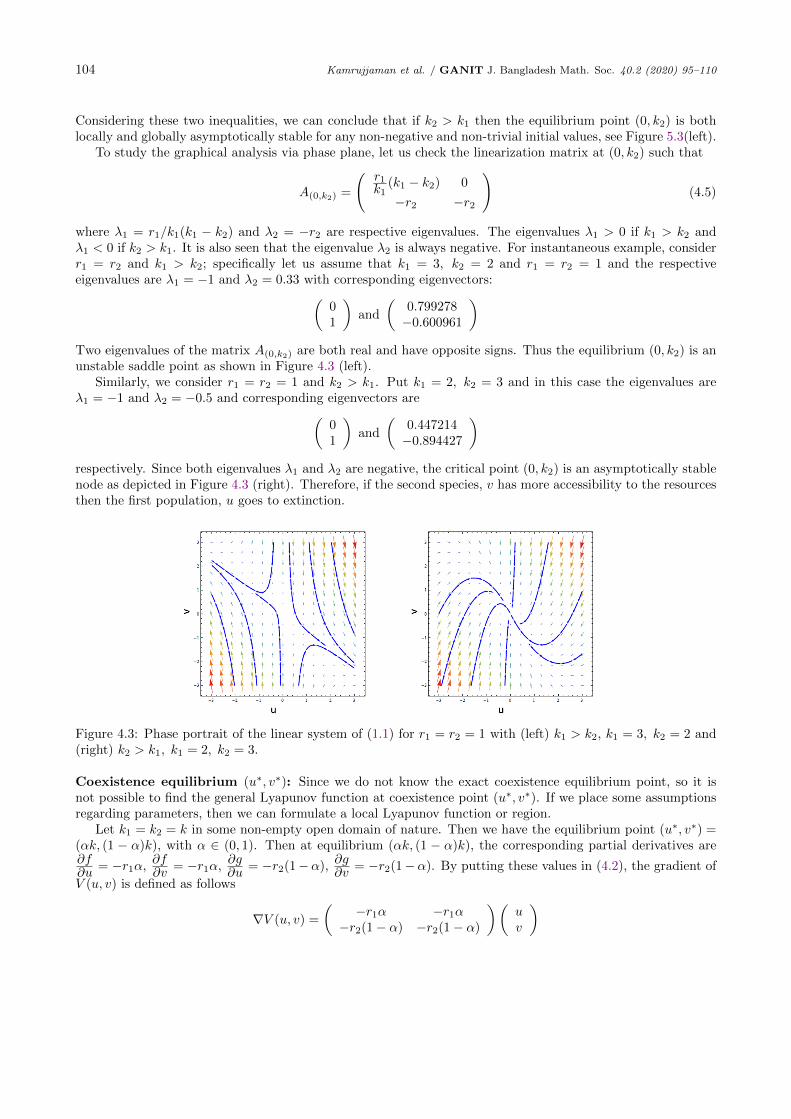
)Two eigenvalues of the matrix A(0,k2) are both real and have opposite signs. Thus the equilibrium (0, k2) is anunstable saddle point as shown in Figure 4.3 (left).

Similarly, we consider r1 = r2 = 1 and k2 > k1. Put k1 = 2, k2 = 3 and in this case the eigenvalues areλ1 = −1 and λ2 = −0.5 and corresponding eigenvectors are(

01

)and

(0.447214−0.894427

)respectively. Since both eigenvalues λ1 and λ2 are negative, the critical point (0, k2) is an asymptotically stablenode as depicted in Figure 4.3 (right). Therefore, if the second species, v has more accessibility to the resourcesthen the first population, u goes to extinction.

Figure 4.3: Phase portrait of the linear system of (1.1) for r1 = r2 = 1 with (left) k1 > k2, k1 = 3, k2 = 2 and(right) k2 > k1, k1 = 2, k2 = 3.

Coexistence equilibrium (u∗, v∗): Since we do not know the exact coexistence equilibrium point, so it isnot possible to find the general Lyapunov function at coexistence point (u∗, v∗). If we place some assumptionsregarding parameters, then we can formulate a local Lyapunov function or region.

Let k1 = k2 = k in some non-empty open domain of nature. Then we have the equilibrium point (u∗, v∗) =(αk, (1 − α)k), with α ∈ (0, 1). Then at equilibrium (αk, (1 − α)k), the corresponding partial derivatives are∂f∂u

= −r1α,∂f∂v

= −r1α,∂g∂u

= −r2(1−α),∂g∂v

= −r2(1−α). By putting these values in (4.2), the gradient of

V (u, v) is defined as follows

∇V (u, v) =

(−r1α −r1α

−r2(1− α) −r2(1− α)

)(uv

)


=

(−r1α(u+ v)

−r2(1− α)(u+ v)

)Integrating ∇V provides the following Lyapunov function V such that

V (u, v) =

u∫0

(−r1α)x dx+

v∫0

(−r2(1− α))y dy

= −r1αu2

2− r2(1− α)

v2

2

Regarding the stability analysis, we must find the criterion such that V is always positive. Assume r1 = r2 = rand V > 0 implies

− rαu2

2− r(1− α)

v2

2> 0

⇒ −α(1− α)

>v2

u2

⇒ −α(1− α)

> 0, while u > 0, v > 0

⇒ 1− α > 0⇒ 0 < α < 1

So V will be positive for α ∈ (0, 1), which was our primary assumption of coexistence solution. To check thelocal or global stability of the coexistence solution, differentiate the function V , and we have

∂V

∂t= −r1αu

du

dt− r2(1− α)v

dv

dt

= −r21

kα(ku2 − u3 − vu2)− r22

k(1− α)(kv2 − uv2 − v3)

For satisfying the Lyapunov strategy, the necessary condition is ∂V∂t

< 0 and hence, either

− r21kα(ku2 − u3 − vu2) < 0

⇒ k >u3 + vu2

u2

Or

− r22k

(1− α)(kv2 − uv2 − v3) < 0

⇒ k >uv2 + v3

v2

Considering these two conditions it can be illuminated that when α ∈ (0, 1), the equilibrium point (αk, (1−α)k)is globally asymptotically stable, see Figure 5.3(middle).

Consider the linearization matrix at (αk, (1− α)k) such that

A(αk,(1−α)k) =

(−r1α −r1α

−r2(1− α) −r2(1− α)

)(4.6)

where λ1 = 0 and λ2 = −(r1α+ r2(1− α)) are respective eigenvalues. Since one eigenvalue is zero, so here wedo not have any point attractor or a point from which it will be repelled.

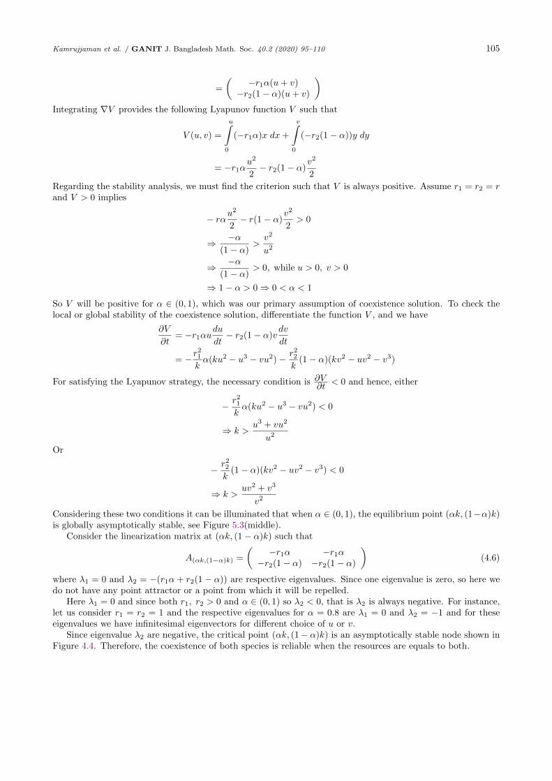
Here λ1 = 0 and since both r1, r2 > 0 and α ∈ (0, 1) so λ2 < 0, that is λ2 is always negative. For instance,let us consider r1 = r2 = 1 and the respective eigenvalues for α = 0.8 are λ1 = 0 and λ2 = −1 and for theseeigenvalues we have infinitesimal eigenvectors for different choice of u or v.

Since eigenvalue λ2 are negative, the critical point (αk, (1− α)k) is an asymptotically stable node shown inFigure 4.4. Therefore, the coexistence of both species is reliable when the resources are equals to both.


Figure 4.4: Phase portrait of the linear system of (1.1) for r1 = r2 = 1 and k1 = k2 = 1 with (left) α = 0.8, and(right) α = 0.5.

5 Numerical Results and Discussions

In this section, we discuss some examples of numerical solutions of the initial value problem (IVP) (1.1).The parameters like specific growth and resource function play a significant role to change population density.

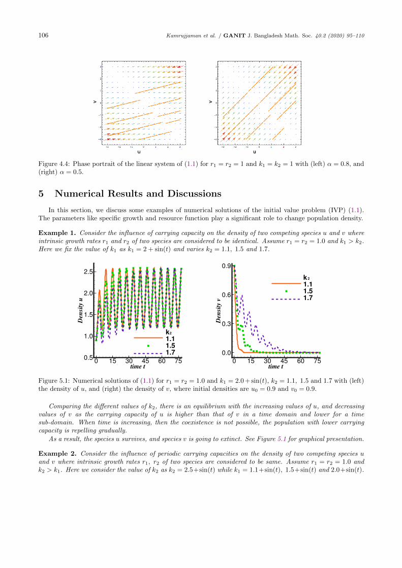
Example 1. Consider the influence of carrying capacity on the density of two competing species u and v whereintrinsic growth rates r1 and r2 of two species are considered to be identical. Assume r1 = r2 = 1.0 and k1 > k2.Here we fix the value of k1 as k1 = 2 + sin(t) and varies k2 = 1.1, 1.5 and 1.7.

time t

Den

sity

u

0 15 30 45 60 750.5

1.0

1.5

2.0

2.5

k

1.1

1.5

1.7

2

time t

Den

sity

v

0 15 30 45 60 75

0.0

0.3

0.6

0.9

k

1.1

1.5

1.7

2

Figure 5.1: Numerical solutions of (1.1) for r1 = r2 = 1.0 and k1 = 2.0 + sin(t), k2 = 1.1, 1.5 and 1.7 with (left)the density of u, and (right) the density of v, where initial densities are u0 = 0.9 and v0 = 0.9.

Comparing the different values of k2, there is an equilibrium with the increasing values of u, and decreasingvalues of v as the carrying capacity of u is higher than that of v in a time domain and lower for a timesub-domain. When time is increasing, then the coexistence is not possible, the population with lower carryingcapacity is repelling gradually.

As a result, the species u survives, and species v is going to extinct. See Figure 5.1 for graphical presentation.

Example 2. Consider the influence of periodic carrying capacities on the density of two competing species uand v where intrinsic growth rates r1, r2 of two species are considered to be same. Assume r1 = r2 = 1.0 andk2 > k1. Here we consider the value of k2 as k2 = 2.5+sin(t) while k1 = 1.1+sin(t), 1.5+sin(t) and 2.0+sin(t).


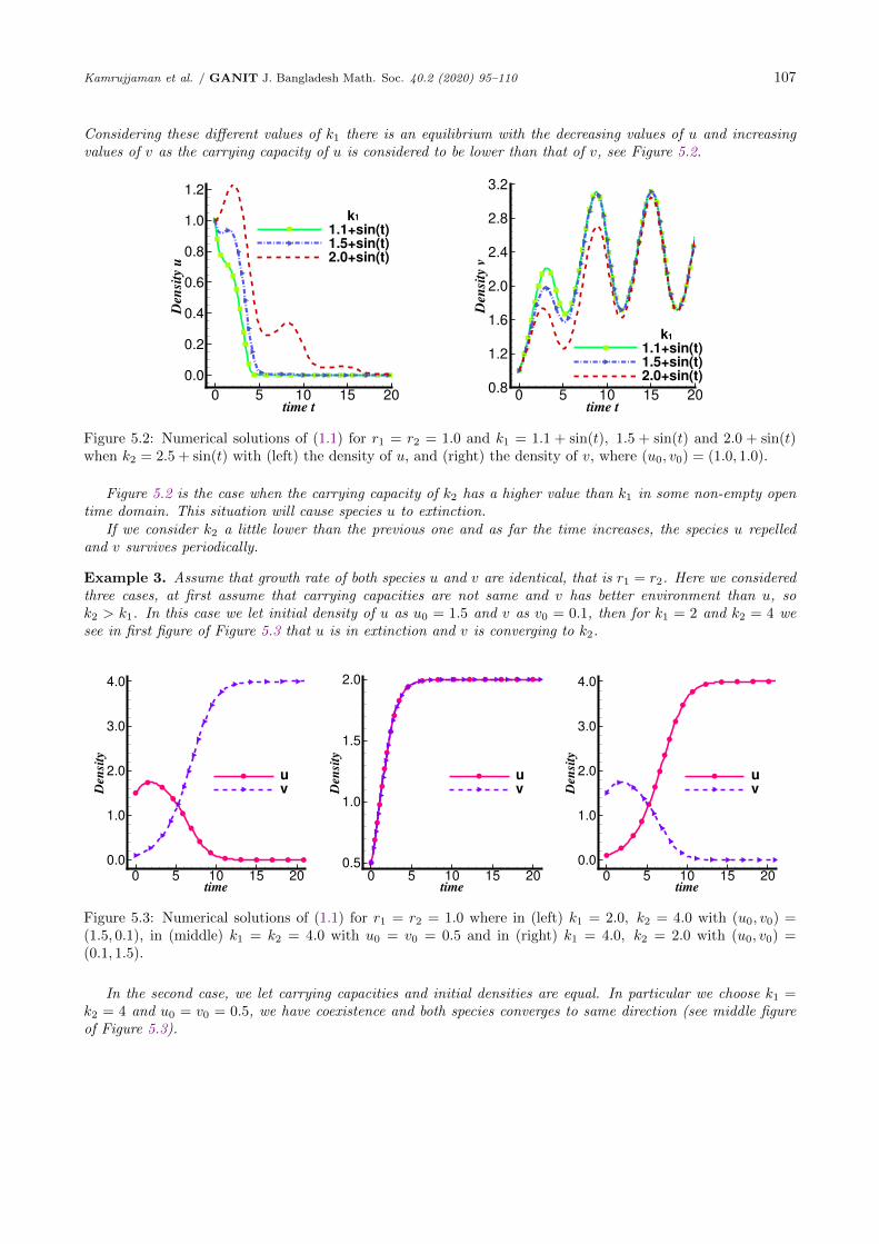
Considering these different values of k1 there is an equilibrium with the decreasing values of u and increasingvalues of v as the carrying capacity of u is considered to be lower than that of v, see Figure 5.2.

time t

Den

sity

u

0 5 10 15 20

0.0

0.2

0.4

0.6

0.8

1.0

1.2

k1.1+sin(t)1.5+sin(t)2.0+sin(t)

1

time t

Den

sity

v

0 5 10 15 200.8

1.2

1.6

2.0

2.4

2.8

3.2

k1.1+sin(t)1.5+sin(t)2.0+sin(t)

1

Figure 5.2: Numerical solutions of (1.1) for r1 = r2 = 1.0 and k1 = 1.1 + sin(t), 1.5 + sin(t) and 2.0 + sin(t)when k2 = 2.5 + sin(t) with (left) the density of u, and (right) the density of v, where (u0, v0) = (1.0, 1.0).

Figure 5.2 is the case when the carrying capacity of k2 has a higher value than k1 in some non-empty opentime domain. This situation will cause species u to extinction.

If we consider k2 a little lower than the previous one and as far the time increases, the species u repelledand v survives periodically.

Example 3. Assume that growth rate of both species u and v are identical, that is r1 = r2. Here we consideredthree cases, at first assume that carrying capacities are not same and v has better environment than u, sok2 > k1. In this case we let initial density of u as u0 = 1.5 and v as v0 = 0.1, then for k1 = 2 and k2 = 4 wesee in first figure of Figure 5.3 that u is in extinction and v is converging to k2.

time

Den

sity

0 5 10 15 20

0.0

1.0

2.0

3.0

4.0

u

v

time

Den

sity

0 5 10 15 20

0.5

1.0

1.5

2.0

u

v

time

Den

sity

0 5 10 15 20

0.0

1.0

2.0

3.0

4.0

u

v

Figure 5.3: Numerical solutions of (1.1) for r1 = r2 = 1.0 where in (left) k1 = 2.0, k2 = 4.0 with (u0, v0) =(1.5, 0.1), in (middle) k1 = k2 = 4.0 with u0 = v0 = 0.5 and in (right) k1 = 4.0, k2 = 2.0 with (u0, v0) =(0.1, 1.5).

In the second case, we let carrying capacities and initial densities are equal. In particular we choose k1 =k2 = 4 and u0 = v0 = 0.5, we have coexistence and both species converges to same direction (see middle figureof Figure 5.3).


Lastly we consider the contrary case of the first one. We assumed that k1 > k2 and by choosing k1 = 4,k2 = 2 and initial densities as (u0, v0) = (0.1, 1.5) then in the last figure of Figure 5.3 shows that one speciesis in extinction and the another one is converging towards carrying capacity. For this properties species v is inextinction and species u converges to k1.

Example 4. Consider the equal carrying capacities for both species; for example, k1 = k2 = 2.0 + sin(t). Herewe show that the effects of intrinsic growth rates on the density of populations by varying growth rates for eachspecies.

time t

Den

sity

u

0 5 10 15 20 25 30

0.6

1.2

1.8

2.4

r =4.01

r

1.0

2.0

3.5

2

time t

Den

sity

v0 5 10 15 20 25 30

0.6

0.9

1.2

1.5

1.8

r =4.01

r

1.0

2.0

3.5

2

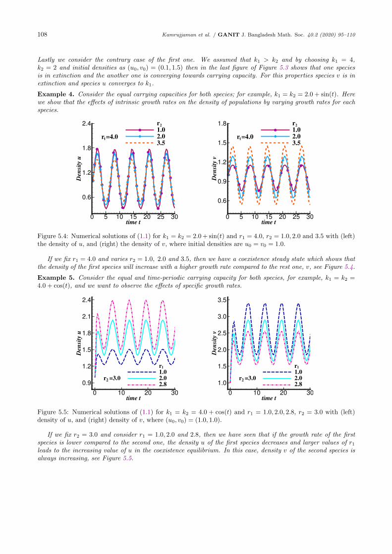
Figure 5.4: Numerical solutions of (1.1) for k1 = k2 = 2.0 + sin(t) and r1 = 4.0, r2 = 1.0, 2.0 and 3.5 with (left)the density of u, and (right) the density of v, where initial densities are u0 = v0 = 1.0.

If we fix r1 = 4.0 and varies r2 = 1.0, 2.0 and 3.5, then we have a coexistence steady state which shows thatthe density of the first species will increase with a higher growth rate compared to the rest one, v, see Figure 5.4.

Example 5. Consider the equal and time-periodic carrying capacity for both species, for example, k1 = k2 =4.0 + cos(t), and we want to observe the effects of specific growth rates.

time t

Den

sity

u

0 10 20 30

0.9

1.2

1.5

1.8

2.1

2.4

r1.02.02.8

1

r =3.02

time t

Den

sity

v

0 10 20 30

1.0

1.5

2.0

2.5

3.0

3.5

r1.02.02.8

1

r =3.02

Figure 5.5: Numerical solutions of (1.1) for k1 = k2 = 4.0 + cos(t) and r1 = 1.0, 2.0, 2.8, r2 = 3.0 with (left)density of u, and (right) density of v, where (u0, v0) = (1.0, 1.0).

If we fix r2 = 3.0 and consider r1 = 1.0, 2.0 and 2.8, then we have seen that if the growth rate of the firstspecies is lower compared to the second one, the density u of the first species decreases and larger values of r1leads to the increasing value of u in the coexistence equilibrium. In this case, density v of the second species isalways increasing, see Figure 5.5.


6 Conclusions

In this paper, we studied a two-species competition population model both analytically and numerically.The results were presented for local and global cases using phase diagrams and periodic functions. It was seenthat in many cases it is possible to determine whether an equilibrium of a nonlinear system is locally stableor globally asymptotically stable simply by Lyapunov’s theorem. This method relies on the observation thatasymptotic stability is intimately linked to the existence of a Lyapunov function. The system is asymptoticallystable means that the equilibrium state at the origin is asymptotically stable, if and only if the eigenvalues havenegative real parts. By this stability analysis, we will get a clear conception about the growth and extinctionof various competitive species. Numerical investigations both confirmed and completed the theoretical resultswhile comparing the density of two different species. Here we have seen that the considered model suggests thatcarrying capacity plays an important role in the determination of the competition outcome between two speciesin a given ecological circumference. If the carrying capacity remains the same for two species, the populationwith a larger growth rate grows high and the population with a smaller growth rate decreases gradually. Whengrowth rates are considered identical, the population with a larger carrying capacity has higher density and isthe sole winner. Dynamical behavior of the system was investigated at equilibrium points. As one parameter isvaried, the dynamics of the system near to this solution change the stability. Both analytically and numerically,the results showed that the model sensitively depends on the parameter values and initial conditions. For futurestudies, it would be interesting if one can study these models for particular species in any habitats.

Acknowledgments

The authors are grateful to the anonymous reviewers for their constructive suggestions to improve the qualityof the paper significantly. The research was partially supported by TWAS grant: 2019 19−169 RG/MATHS/AS I.

References

[1] Gilpin, M. E., Ayala, F. J., Global models of growth and competition, Proc Natl Acad Sci USA, 70(12):3590-3593 (1973).

[2] Protter, M. H., Weinberger, H. F., Maximum Principles in Differential Equations, Prentice Hall, Inc.,Englewood Cliffs, N.J. (1967).

[3] Smith, H. L., Monotone Dynamical Systems: An Introduction to the Theory of Competitive and Coop-erative Systems, American Mathematical Society, Providence, RI, 41 (1995).

[4] Gopalsamy, K., Exchange of equilibria in two species Lotka-Volterra competition models, J. Austral. Math.Soc. (Series B), 24(2): 160-170 (1982).

[5] Sun, J., Zhang, D., Wu, B., Qualitative properties of cooperative degenerate Lotka-volterra model, Ad-vances in Difference Equations, 281 (2013).

[6] Hsu, S. B., Smith, H. L., Waltman, P., Competitive exclusion and coexistence for competitive systems onordered Banach spaces, Trans. Amer. Math. Soc., 348(10): 4083–4094 (1996).

[7] Dancer, E. N., Positivity of maps and applications, Topological Nonlinear Analysis, Chapter Part of theProgress in Nonlinear Differential Equations and Their Applications book series (15), 303–340, (1995).

[8] Lam, K. Y., Munther, D., A remark on the global dynamics of competitive systems on ordered Banachspaces, Proc. Am. Math. Soc., 144: 1153–1159 (2015).

[9] Braverman, E., Kamrujjaman, M., Korobenko, L., Competitive spatially distributed population dynamicsmodels: Does diversity in diffusion strategies promote coexistence? Math. Biosci., 264: 63–73 (2015).


[10] Murray, J. D., Mathematical Biology: I An Introduction, Springer-Verlag (2002).

[11] Sun, G. Q., Mathematical modeling of population dynamics with Allee effect, Nonlinear Dynamics, 85:1–12 (2016).

[12] Wittmann, M. J., Stuis, H., Metzler, D., Genetic Allee effects and their interaction with ecological Alleeeffects, Journal of Animal Ecology, 87(1): 11–23 (2016).

[13] Liu, X., Fan, G., Zhang T., Evolutionary dynamics of single species model with Allee effect, Physica A,526: 120774 (2019).

[14] Morgan, R., Linearization and Stability Analysis of Nonlinear Problems, Rose-Hulman UndergraduateMathematics Journal, 16(2): 66-91, Article 5 (2015).

[15] Hirsch, M. W., Smale, S., Devaney, R. L., Differential Equations, Dynamical Systems, and An introductionto Chaos, Elsevier Academic Press, USA (2004).

[16] Guckenheimer, J., Holmes, P., Nonlinear Oscillations, Dynamical Systems, and Bifurcations of VectorFields, Springer-Verlag, New York (1983).

[17] Huu, K. N., Stability analysis in competition population model, Int. J. Math. Models and Methods inApplied sciences, 6(1): 11-19 (2012).

[18] Hartman, P., A lemma in the theory of structural stability of differential equations, Proceedings of theAMS, 11: 610–620 (1960).

[19] Bicout, D. J., Linear Stability Analysis, EPSP-TIMC, UMR 5525 (2013).

[20] Eberly, D., Stability analysis for systems of differential equations, CA 94042, USA (2008).

[21] Kamrujjaman, M., Interplay of Resource Distributions and Diffusion Strategies for Spatially Heteroge-neous Populations, J. Mathematical Modeling, 7(2): 175–198 (2019).

[22] Kamrujjaman, M., Directed vs Regular Diffusion Strategy: Evolutionary Stability Analysis of a Compe-tition Model and an Ideal Free Pair, Differential Equations and Applications, 11(2): 267–290 (2019).

[23] Kamrujjaman, M., Ahmed, A., Ahmed S., Competitive Reaction-Diffusion Systems: Traveling Waves andNumerical Solutions, Advances in Research, 19(6): 1–12 (2019).

[24] Kamrujjaman, M., Weak Competition and Ideally Distributed Populations in a Cooperative DiffusiveModel with Crowding Effects, Physical Science International Journal, 18(4): 1–16 (2018).

[25] Kamrujjaman, M., Keya K. N., Global Analysis of a Directed Dynamics Competition Model, J. Advancesin Mathematics and Computer Science, 27(2): 1–14 (2018).

[26] Kamrujjaman, M., Dispersal Dynamics: Competitive Symbiotic and Predator-Prey Interactions, J. Ad-vanced Mathematics and Applications, 6: 7–17 (2017).

[27] Perko, L., Differential Equations and dynamical Systems, Springer (2008).

[28] LaSalle, J. P., The stability of dynamical system, Regional Conference Series in Applied Mathematics,SIAM, Philadelphia (1976).

[29] Wiggins, S., Introduction to Applied Nonlinear Dynamical Systems and Chaos, Springer-Verlag, NewYork (1983).

Lyapunov Stability Analysis of a Competition Model with ...

Documents