Learning Control Lyapunov Function to Ensure Stability of ...lasa.epfl.ch/publications/uploadedFiles/Khansari_Billard_RAS2014.pdf · Learning Control Lyapunov Function to Ensure Stability

Learning Control Lyapunov Function to EnsureStability of Dynamical System-based Robot Reaching Motions

S. Mohammad Khansari-Zadeh∗, Aude Billard1

EPFL-STI-IMT-LASA, CH-1015, Lausanne, Switzerland

Abstract

We consider an imitation learning approach to model robot point-to-point (also known as discrete or reaching) movements with aset of autonomous Dynamical Systems (DS). Each DS model codes a behavior (such as reaching for a cup and swinging a golfclub) at the kinematic level. An estimate of these DS models are usually obtained from a set of demonstrations of the task. Whenmodeling robot discrete motions with DS, ensuring stability of the learned DS is a key requirement to provide a useful policy.In this paper we propose an imitation learning approach that exploits the power of Control Lyapunov Function (CLF) controlscheme to ensure global asymptotic stability of nonlinear DS. Given a set of demonstrations of a task, our approach proceeds inthree steps: 1) Learning a valid Lyapunov function from the demonstrations by solving a constrained optimization problem, 2)Using one of the-state-of-the-art regression techniques to model an (unstable) estimate of the motion from the demonstrations,and 3) Using (1) to ensure stability of (2) during the task execution via solving a constrained convex optimization problem. Theproposed approach allows learning a larger set of robot motions compared to existing methods that are based on quadratic Lyapunovfunctions. Additionally, by using the CLF formalism, the problem of ensuring stability of DS motions becomes independent fromthe choice of regression method. Hence it allows the user to adopt the most appropriate technique based on the requirements of thetask at hand without compromising stability. We evaluate our approach both in simulation and on the 7 degrees of freedom BarrettWAM arm.

Keywords: Robot point-to-point Movements, Imitation Learning, Control Lyapunov Function, Nonlinear dynamical systems,Stability Analysis, Movement Primitives

1. Introduction

When designing robots meant to interact in a human environ-ment, it is essential to develop methods that can easily transferskills from nonexpert users to robots, and at the same time, pro-vide the required robustness and reactivity to interact with adynamic environment. Classical approaches to modeling robotmotions rely on decomposing the task execution into two sepa-rate processes:planningandexecution[1]. The former is usedas a means to generate a feasible path that can satisfy the task’srequirements, and the latter is designed so that it follows thegenerated feasible path as closely as possible. Hence these ap-proaches consider any deviation from the desired path (due toperturbations or changes in environment) as the tracking error,and various control theories have been developed to efficientlysuppress this error in terms of some objective functions. De-spite the great success of these approaches in providing power-ful robotic systems, particularly in factories, they are ill-suitedfor robotic systems that are aimed to work in the close vicinityof humans, and thus alternative techniques must be sought.

∗Ecole Polytechnique Federale de Lausanne, LASA Laboratory, Switzerland.Email addresses:[email protected](S. Mohammad Khansari-Zadeh),

[email protected](A. Billard)URL: http://lasa.epfl.ch/

1Ecole Polytechnique Federale de Lausanne, LASA Laboratory, Switzerland.

In robotics, Dynamical Systems (DS) based approaches tomotion generation have been shown to be interesting alterna-tives to classical methods as they offer a natural means to in-tegrate planning and execution into one single unit [2, 3, 4, 5].For instance when modeling robot reaching motions with DS,all possible solutions to reach the target are embedded into onesingle model [6]. Such a model represents a global map whichspecifiesinstantlythe correct direction for reaching the target,considering the current state of the robot, the target, and all theother objects in the robot’s working space. Such models aremore similar to human movements in that they can effortlesslyadapt its motion to changes in the environment rather than stub-bornly following the previous path [6, 7, 8, 9, 10, 11, 12]. Inother words, the main advantage of using DS-based formulationcan be summarized as: “Modeling movements with DS allowshaving robotic systems that have inherent adaptivity to changesin a dynamic environment, and that can swiftly adopt a newpath to reach the target”. This advantage is the direct outcomeof having a unified planning and execution unit.

Imitation learning (also known as learning from demonstra-tions) is one of the most common and intuitive ways of build-ing an estimate of DS motions from a set of demonstrations[6, 13, 7, 8]. When modeling robot motions with DS,ensuringstability of the estimated DS – ensuring the robot reaches thefinal desired state – is one of the main challenges that should

Accepted in Robotics and Autonomous Systems March 3, 2014

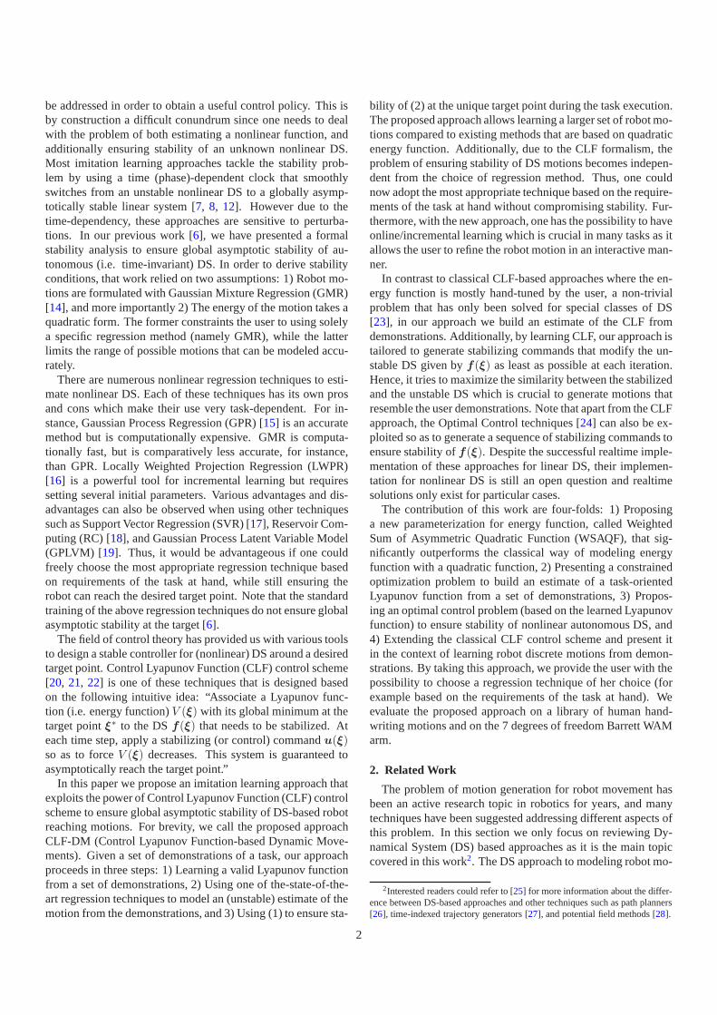
be addressed in order to obtain a useful control policy. This isby construction a difficult conundrum since one needs to dealwith the problem of both estimating a nonlinear function, andadditionally ensuring stability of an unknown nonlinear DS.Most imitation learning approaches tackle the stability prob-lem by using a time (phase)-dependent clock that smoothlyswitches from an unstable nonlinear DS to a globally asymp-totically stable linear system [7, 8, 12]. However due to thetime-dependency, these approaches are sensitive to perturba-tions. In our previous work [6], we have presented a formalstability analysis to ensure global asymptotic stability of au-tonomous (i.e. time-invariant) DS. In order to derive stabilityconditions, that work relied on two assumptions: 1) Robot mo-tions are formulated with Gaussian Mixture Regression (GMR)[14], and more importantly 2) The energy of the motion takes aquadratic form. The former constraints the user to using solelya specific regression method (namely GMR), while the latterlimits the range of possible motions that can be modeled accu-rately.

There are numerous nonlinear regression techniques to esti-mate nonlinear DS. Each of these techniques has its own prosand cons which make their use very task-dependent. For in-stance, Gaussian Process Regression (GPR) [15] is an accuratemethod but is computationally expensive. GMR is computa-tionally fast, but is comparatively less accurate, for instance,than GPR. Locally Weighted Projection Regression (LWPR)[16] is a powerful tool for incremental learning but requiressetting several initial parameters. Various advantages and dis-advantages can also be observed when using other techniquessuch as Support Vector Regression (SVR) [17], Reservoir Com-puting (RC) [18], and Gaussian Process Latent Variable Model(GPLVM) [19]. Thus, it would be advantageous if one couldfreely choose the most appropriate regression technique basedon requirements of the task at hand, while still ensuring therobot can reach the desired target point. Note that the standardtraining of the above regression techniques do not ensure globalasymptotic stability at the target [6].

The field of control theory has provided us with various toolsto design a stable controller for (nonlinear) DS around a desiredtarget point. Control Lyapunov Function (CLF) control scheme[20, 21, 22] is one of these techniques that is designed basedon the following intuitive idea: “Associate a Lyapunov func-tion (i.e. energy function)V (ξ) with its global minimum at thetarget pointξ∗ to the DSf(ξ) that needs to be stabilized. Ateach time step, apply a stabilizing (or control) commandu(ξ)so as to forceV (ξ) decreases. This system is guaranteed toasymptotically reach the target point.”

In this paper we propose an imitation learning approach thatexploits the power of Control Lyapunov Function (CLF) controlscheme to ensure global asymptotic stability of DS-based robotreaching motions. For brevity, we call the proposed approachCLF-DM (Control Lyapunov Function-based Dynamic Move-ments). Given a set of demonstrations of a task, our approachproceeds in three steps: 1) Learning a valid Lyapunov functionfrom a set of demonstrations, 2) Using one of the-state-of-the-art regression techniques to model an (unstable) estimate of themotion from the demonstrations, and 3) Using (1) to ensure sta-

bility of (2) at the unique target point during the task execution.The proposed approach allows learning a larger set of robot mo-tions compared to existing methods that are based on quadraticenergy function. Additionally, due to the CLF formalism, theproblem of ensuring stability of DS motions becomes indepen-dent from the choice of regression method. Thus, one couldnow adopt the most appropriate technique based on the require-ments of the task at hand without compromising stability. Fur-thermore, with the new approach, one has the possibility to haveonline/incremental learning which is crucial in many tasks as itallows the user to refine the robot motion in an interactive man-ner.

In contrast to classical CLF-based approaches where the en-ergy function is mostly hand-tuned by the user, a non-trivialproblem that has only been solved for special classes of DS[23], in our approach we build an estimate of the CLF fromdemonstrations. Additionally, by learning CLF, our approach istailored to generate stabilizing commands that modify the un-stable DS given byf(ξ) as least as possible at each iteration.Hence, it tries to maximize the similarity between the stabilizedand the unstable DS which is crucial to generate motions thatresemble the user demonstrations. Note that apart from the CLFapproach, the Optimal Control techniques [24] can also be ex-ploited so as to generate a sequence of stabilizing commands toensure stability off(ξ). Despite the successful realtime imple-mentation of these approaches for linear DS, their implemen-tation for nonlinear DS is still an open question and realtimesolutions only exist for particular cases.

The contribution of this work are four-folds: 1) Proposinga new parameterization for energy function, called WeightedSum of Asymmetric Quadratic Function (WSAQF), that sig-nificantly outperforms the classical way of modeling energyfunction with a quadratic function, 2) Presenting a constrainedoptimization problem to build an estimate of a task-orientedLyapunov function from a set of demonstrations, 3) Propos-ing an optimal control problem (based on the learned Lyapunovfunction) to ensure stability of nonlinear autonomous DS, and4) Extending the classical CLF control scheme and present itin the context of learning robot discrete motions from demon-strations. By taking this approach, we provide the user with thepossibility to choose a regression technique of her choice (forexample based on the requirements of the task at hand). Weevaluate the proposed approach on a library of human hand-writing motions and on the 7 degrees of freedom Barrett WAMarm.

2. Related Work

The problem of motion generation for robot movement hasbeen an active research topic in robotics for years, and manytechniques have been suggested addressing different aspects ofthis problem. In this section we only focus on reviewing Dy-namical System (DS) based approaches as it is the main topiccovered in this work2. The DS approach to modeling robot mo-

2Interested readers could refer to [25] for more information about the differ-ence between DS-based approaches and other techniques such as path planners[26], time-indexed trajectory generators [27], and potential field methods [28].

2

ξ1

ξ2

Swing Motion

Resting Motion

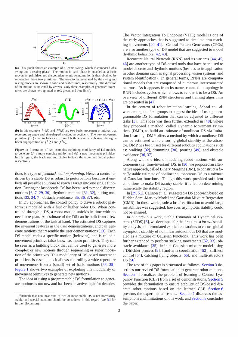
(a) This graph shows an example of a tennis swing, which is composed of aswing and a resting phase. The motion in each phase is encoded as a basicmovement primitive, and the complete tennis swing motion is thus obtained bysequencing these two primitives. The trajectories generated by the swing andresting models are shown in solid and dashed lines, respectively. The directionof the motion is indicated by arrows. Only three examples of generated trajec-tories are shown here (plotted as red, green, and blue lines).

−0.2 −0.15 −0.1 −0.05 0

0

0.05

0.1

ξ1(m)

ξ2(m

)

f 1(ξ)

−0.3 −0.2 −0.1 0−0.1

−0.05

0

0.05

0.1

ξ1(m)

ξ2(m

)

f 2(ξ)

−0.3 −0.2 −0.1 0

0

0.05

0.1

0.15

ξ1(m)

ξ2(m

)

f 3(ξ) = 0.8f 1(ξ) + f 2(ξ)

(b) In this examplef1(ξ) andf2(ξ) are two basic movement primitives thatrepresent an angle and sine-shaped motion, respectively. The new movementprimitive f3(ξ) that includes a mixture of both behaviors is obtained through alinear superposition off1(ξ) andf2(ξ).

Figure 1: Illustration of two examples exploiting modularity of DS modelsto generate(a) a more complex motion and(b) a new movement primitive.In this figure, the black star and circles indicate the target and initial points,respectively.

tions is a type offeedback motion planning. Hence a controllerdriven by a stable DS is robust to perturbations because it em-beds all possible solutions to reach a target into one single func-tion. During the last decade, DS has been used to model discretemotions [6, 7, 29, 30], rhythmic motions [31, 32], hitting mo-tions [33, 34, 7], obstacle avoidance [35, 36, 37], etc.

In DS approaches, the control policy to drive a robotic plat-form is modeled with a first or higher order DS. When con-trolled through a DS, a robot motion unfolds in time with noneed to re-plan. An estimate of the DS can be built from a fewdemonstrations of the task at hand. The estimated DS capturesthe invariant features in the user demonstrations, and can gen-erate motions that resemble the user demonstrations [13]. EachDS model codes a specific motion (behavior), and is called amovement primitive (also known as motor primitive). They canbe seen as a building block that can be used to generate morecomplex or new motions through sequencing or superimposi-tion of the primitives. This modularity of DS-based movementprimitives is essential as it allows controlling a wide repertoireof movements from a (small) set of basic motions [38, 39].Figure 1shows two examples of exploiting this modularity ofmovement primitives to generate new motions3.

The idea of using a programmable DS formulation to gener-ate motions is not new and has been an active topic for decades.

3Remark that nonlinear sum of two or more stable DS is not necessarilystable, and special attention should be considered in this regard (see [6] forfurther discussion).

The Vector Integration To Endpoint (VITE) model is one ofthe early approaches that is suggested to simulate arm reach-ing movements [40, 41]. Central Pattern Generators (CPGs)are also another type of DS model that are suggested to modelrhythmic behaviors [42, 43].

Recurrent Neural Network (RNN) and its variants [44, 45,46] are another type of DS-based tools that have been used tomodel discrete and rhythmic motions (besides to its applicationin other domains such as signal processing, vision systems, andsystem identification). In general terms, RNNs are computa-tional models that are composed of numerous interconnectedneurons. As it appears from its name, connection topology inRNN includes cycles which allows to render it to be a DS. Anoverview of different RNN structures and training algorithmsare presented in [47].

In the context of robot imitation learning, Schaal et. al.were among the first groups to suggest the idea of using a pro-grammable DS formulation that can be adjusted to differenttasks [3]. This idea was then further extended in [48], wherethey proposed a method, called Dynamic Movement Primi-tives (DMP), to build an estimate of nonlinear DS via Imita-tion Learning. DMP offers a method by which a nonlinear DScan be estimated while ensuring global stability at the attrac-tor. DMP has been used for different robotics applications suchas: walking [32], drumming [30], pouring [49], and obstacleavoidance [36, 37].

Along with the idea of modeling robot motions with au-tonomous (i.e. time-invariant) DS, in [50] we proposed an alter-native approach, called Binary Merging (BM), to construct alo-cally stable estimate of nonlinear autonomous DS as a mixtureof Gaussian functions. Though this work provided sufficientconditions to make DSlocally stable, it relied on determiningnumerically the stability region.

In [29, 51], Calinon et. al. suggested a DS approach based onHidden Semi-Markov Model and Gaussian Mixture Regression(GMR). In these works, sole a brief verification to avoid largeinstabilities was suggested; however, asymptotic stability couldnot be ensured.

In our previous work, Stable Estimator of Dynamical sys-tems (SEDS) [6], we developed for the first time aformalstabil-ity analysis and formulated explicit constraints to ensure globalasymptotic stability of nonlinear autonomous DS that are mod-eled as a mixture of Gaussian functions. This work has beenfurther extended to perform striking movements [52, 33], ob-stacle avoidance [35], infinite Gaussian mixture model usinga Dirichlet process [9], hand-arm coordination [53], stiffnesscontrol [54], catching flying objects [55], and multi-attractorsDS [56].

The rest of this paper is structured as follows:Section 3de-scribes our revised DS formulation to generate robot motions.Section 4formalizes the problem of learning a Control Lya-punov Function (CLF) from a set of demonstrations.Section 5provides the formulation to ensure stability of DS-based dis-crete robot motions based on the learned CLF.Section 6presents the experimental results.Section 7discusses the as-sumptions and limitations of this work, andSection 8concludesthe paper.

3

ξ1

ξ2

Initial PointTarget PointUnstable Generated TrajectorySpurious attractors

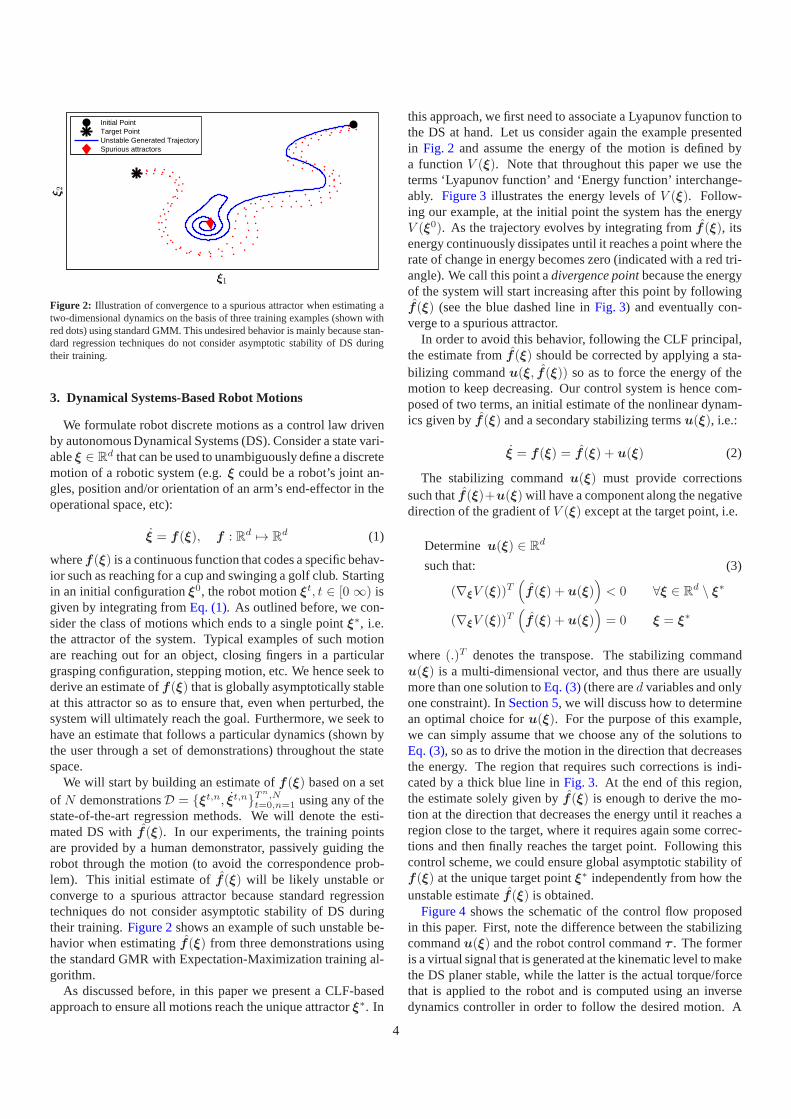
Figure 2: Illustration of convergence to a spurious attractor when estimating atwo-dimensional dynamics on the basis of three training examples (shown withred dots) using standard GMM. This undesired behavior is mainly because stan-dard regression techniques do not consider asymptotic stability of DS duringtheir training.

3. Dynamical Systems-Based Robot Motions

We formulate robot discrete motions as a control law drivenby autonomous Dynamical Systems (DS). Consider a state vari-ableξ ∈ R

d that can be used to unambiguously define a discretemotion of a robotic system (e.g.ξ could be a robot’s joint an-gles, position and/or orientation of an arm’s end-effector in theoperational space, etc):

ξ = f(ξ), f : Rd 7→ Rd (1)

wheref(ξ) is a continuous function that codes a specific behav-ior such as reaching for a cup and swinging a golf club. Startingin an initial configurationξ0, the robot motionξt, t ∈ [0 ∞) isgiven by integrating fromEq. (1). As outlined before, we con-sider the class of motions which ends to a single pointξ∗, i.e.the attractor of the system. Typical examples of such motionare reaching out for an object, closing fingers in a particulargrasping configuration, stepping motion, etc. We hence seek toderive an estimate off(ξ) that is globally asymptotically stableat this attractor so as to ensure that, even when perturbed, thesystem will ultimately reach the goal. Furthermore, we seek tohave an estimate that follows a particular dynamics (shown bythe user through a set of demonstrations) throughout the statespace.

We will start by building an estimate off(ξ) based on a setof N demonstrationsD = {ξt,n, ξt,n}T

n,Nt=0,n=1 using any of the

state-of-the-art regression methods. We will denote the esti-mated DS withf (ξ). In our experiments, the training pointsare provided by a human demonstrator, passively guiding therobot through the motion (to avoid the correspondence prob-lem). This initial estimate off(ξ) will be likely unstable orconverge to a spurious attractor because standard regressiontechniques do not consider asymptotic stability of DS duringtheir training.Figure 2shows an example of such unstable be-havior when estimatingf(ξ) from three demonstrations usingthe standard GMR with Expectation-Maximization training al-gorithm.

As discussed before, in this paper we present a CLF-basedapproach to ensure all motions reach the unique attractorξ∗. In

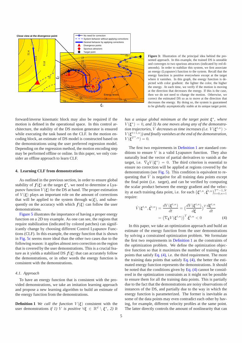
this approach, we first need to associate a Lyapunov function tothe DS at hand. Let us consider again the example presentedin Fig. 2 and assume the energy of the motion is defined bya functionV (ξ). Note that throughout this paper we use theterms ‘Lyapunov function’ and ‘Energy function’ interchange-ably. Figure 3illustrates the energy levels ofV (ξ). Follow-ing our example, at the initial point the system has the energyV (ξ0). As the trajectory evolves by integrating fromf (ξ), itsenergy continuously dissipates until it reaches a point where therate of change in energy becomes zero (indicated with a red tri-angle). We call this point adivergence pointbecause the energyof the system will start increasing after this point by followingf(ξ) (see the blue dashed line inFig. 3) and eventually con-verge to a spurious attractor.

In order to avoid this behavior, following the CLF principal,the estimate fromf(ξ) should be corrected by applying a sta-bilizing commandu(ξ, f(ξ)) so as to force the energy of themotion to keep decreasing. Our control system is hence com-posed of two terms, an initial estimate of the nonlinear dynam-ics given byf(ξ) and a secondary stabilizing termsu(ξ), i.e.:

ξ = f(ξ) = f(ξ) + u(ξ) (2)

The stabilizing commandu(ξ) must provide correctionssuch thatf(ξ)+u(ξ) will have a component along the negativedirection of the gradient ofV (ξ) except at the target point, i.e.

Determineu(ξ) ∈ Rd

such that: (3)

(∇ξV (ξ))T(

f(ξ) + u(ξ))

< 0 ∀ξ ∈ Rd \ ξ∗

(∇ξV (ξ))T(

f(ξ) + u(ξ))

= 0 ξ = ξ∗

where(.)T denotes the transpose. The stabilizing commandu(ξ) is a multi-dimensional vector, and thus there are usuallymore than one solution toEq. (3)(there ared variables and onlyone constraint). InSection 5, we will discuss how to determinean optimal choice foru(ξ). For the purpose of this example,we can simply assume that we choose any of the solutions toEq. (3), so as to drive the motion in the direction that decreasesthe energy. The region that requires such corrections is indi-cated by a thick blue line inFig. 3. At the end of this region,the estimate solely given byf(ξ) is enough to derive the mo-tion at the direction that decreases the energy until it reaches aregion close to the target, where it requires again some correc-tions and then finally reaches the target point. Following thiscontrol scheme, we could ensure global asymptotic stability off(ξ) at the unique target pointξ∗ independently from how theunstable estimatef(ξ) is obtained.

Figure 4shows the schematic of the control flow proposedin this paper. First, note the difference between the stabilizingcommandu(ξ) and the robot control commandτ . The formeris a virtual signal that is generated at the kinematic level to makethe DS planer stable, while the latter is the actual torque/forcethat is applied to the robot and is computed using an inversedynamics controller in order to follow the desired motion. A

4

ξ1

ξ2

9 10

11

1112

12

13

1313

14

14

14

14

15

15

15

15

16

16

1616

17

17

1717

18

18

18

19

1919

2020

No need for correction

System behavior without applying corrections

Desired behavior by applying corrections

Divergence points

Spurious attractors

Target point

Close view at the divergence point

11.4

11.6

11.8

12

Energy levels

Figure 3: Illustration of the principal idea behind the pre-sented approach. In this example, the trained DS is unstableand converges to two spurious attractors (indicated by red di-amonds). In order to stabilize this system, we first associatean energy (Lyapunov) function to the system. Recall that theenergy function is positive everywhere except at the targetwhere it vanishes. In this graph, the energy function is de-picted with color gradient: the lighter the color, the higherthe energy. At each time, we verify if the motion is movingat the direction that decreases the energy. If this is the case,then we do not need to change the motion. Otherwise, wecorrect the estimated DS so as to move at the direction thatdecreases the energy. By doing so, the system is guaranteedto be globally asymptotically stable at its unique target point.

forward/inverse kinematic block may also be required if themotion is defined in the operational space. In this control ar-chitecture, the stability of the DS motion generator is ensuredwhile executing the task based on the CLF. In the motion en-coding block, an estimate of DS model is constructed based onthe demonstrations using the user preferred regression model.Depending on the regression method, the motion encoding stepmay be performed offline or online. In this paper, we only con-sider an offline approach to learn CLF.

4. Learning CLF from demonstrations

As outlined in the previous section, in order to ensure globalstability of f(ξ) at the targetξ∗, we need to determine a Lya-punov functionV (ξ) for the DS at hand. The proper estimationof V (ξ) plays an important role on the amount of correctionsthat will be applied to the system throughu(ξ), and subse-quently on the accuracy with whichf(ξ) can follow the userdemonstrations.

Figure 5illustrates the importance of having a proper energyfunction on a 2D toy example. As one can see, the regions thatrequire stabilization (indicated by colored patches) can signif-icantly change by choosing different Control Lyapunov Func-tions (CLF). In this example, the energy function that is shownin Fig. 5cseems more ideal than the other two cases due to thefollowing reason: it applies almost zero correction on the regionthat is covered by the user demonstrations. This is a crucial fea-ture as it yields a stabilized DSf(ξ) that can accurately followthe demonstrations, or in other words the energy function isconsistent with the demonstrations.

4.1. Approach

To have an energy function that is consistent with the pro-vided demonstrations, we take an imitation learning approachand propose a new learning algorithm to build an estimate ofthe energy function from the demonstrations.

Definition 1 We call the functionV (ξ) consistent with theuser demonstrationsif 1) V is positive∀ξ ∈ R

d \ ξ∗, 2) It

has a unique global minimum at the target pointξ∗, whereV (ξ∗) = 0, and 3) As one moves along any of the demonstra-tion trajectories,V decreases as time increases (i.e.V (ξt,n) >V (ξt+1,n)) and finally vanishes at the end of the demonstration,V (ξT

n,n) = 0.

The first two requirements inDefinition 1are standard con-ditions to ensureV is a valid Lyapunov function. They alsonaturally lead the vector of partial derivatives to vanish at thetarget, i.e. ∇ξV (ξ∗) = 0. The third criterion is essential toensure no correction will be applied at regions covered by thedemonstrations (seeFig. 5). This condition is equivalent to re-questing thatV is negative for all training data points exceptthe final point (i.e. target), and can be verified by computingthe scalar product between the energy gradient and the veloc-ity at each training data point, i.e. for each{ξt,n, ξt,n}T

n−1,Nt=0,n=1

require:

V (ξt,n, ξt,n) =dV (ξt,n)

dt=

(dV (ξt,n)

dξ

)T dξt,n

dt

=(∇ξV (ξt,n)

)Tξt,n < 0 (4)

In this paper, we take an optimization approach and build anestimate of the energy function from the user demonstrationsby solving a constrained optimization problem. We formulatethe first two requirements inDefinition 1 as the constraints ofthe optimization problem. We define the optimization objec-tive function so that it maximizes the number of training datapoints that satisfyEq. (4), i.e. the third requirement. The morethe training data points that satisfyEq. (4), the better the esti-mated energy function represents the demonstrations. It shouldbe noted that the conditions given byEq. (4)cannot be consid-ered in the optimization constraints as it might not be possibleto ensure them for all the training data points. This is partiallydue to the fact that the demonstrations are noisy observations ofinstances of the DS, and partially due to the way in which theenergy function is parameterized. The former is inevitable assome of the data points may even contradict each other by hav-ing, for example, different velocity profiles at the same point.The latter directly controls the amount of nonlinearity that can

5

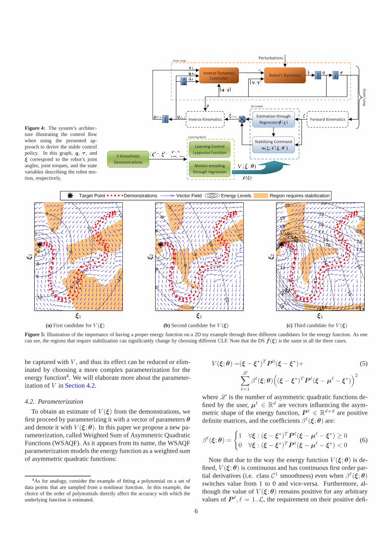
Figure 4: The system’s architec-ture illustrating the control flowwhen using the presented ap-proach to derive the stable controlpolicy. In this graph,q, τ , andξ correspond to the robot’s jointangles, joint torques, and the statevariables describing the robot mo-tion, respectively.

Stabilizing Command

Robot’s Dynamics

Forward KinematicsInverse Kinematics

Inverse Dynamics

Controller

Inner Loop

N Kinesthetic

DemonstrationsMotion encoding

through regression

Ou

ter

Loo

p

Perturbations

Learning Block

Estimation through

Regression

DS model

Learning Control

Lyapunov Function

6778899910101011

11 Target Point Demonstrations Vector Field Energy Levels Region requires stabilization

6

7

7

8

8

9

9

9

10

10

10

11

11

ξ1

ξ2

(a) First candidate forV (ξ)

6

7

7

8

8

8

9

9

9

9

10

10

11

ξ1

ξ2

(b) Second candidate forV (ξ)

910

11

11

12

12

13

13

13

14

14

14

14

15

15

15

15

15

1616

16

16

1616

17

17

17 17

17

18

1818

18

1919

19

2020

20

ξ1

ξ2

(c) Third candidate forV (ξ)

Figure 5: Illustration of the importance of having a proper energy function on a 2D toy example through three different candidates for the energy function. As onecan see, the regions that require stabilization can significantly change by choosing different CLF. Note that the DSf(ξ) is the same in all the three cases.

be captured withV , and thus its effect can be reduced or elim-inated by choosing a more complex parameterization for theenergy function4. We will elaborate more about the parameter-ization ofV in Section 4.2.

4.2. Parameterization

To obtain an estimate ofV (ξ) from the demonstrations, wefirst proceed by parameterizing it with a vector of parametersθ

and denote it withV (ξ; θ). In this paper we propose a new pa-rameterization, called Weighted Sum of Asymmetric QuadraticFunctions (WSAQF). As it appears from its name, the WSAQFparameterization models the energy function as a weighted sumof asymmetric quadratic functions:

4As for analogy, consider the example of fitting a polynomial on a set ofdata points that are sampled from a nonlinear function. In this example, thechoice of the order of polynomials directly affect the accuracy with which theunderlying function is estimated.

V (ξ; θ) =(ξ − ξ∗)TP 0(ξ − ξ∗)+ (5)L∑

ℓ=1

βℓ(ξ; θ)(

(ξ − ξ∗)TP ℓ(ξ − µℓ − ξ∗))2

whereL is the number of asymmetric quadratic functions de-fined by the user,µℓ ∈ R

d are vectors influencing the asym-metric shape of the energy function,P ℓ ∈ R

d×d are positivedefinite matrices, and the coefficientsβℓ(ξ; θ) are:

βℓ(ξ; θ) =

{

1 ∀ξ : (ξ − ξ∗)TP ℓ(ξ − µℓ − ξ∗) ≥ 0

0 ∀ξ : (ξ − ξ∗)TP ℓ(ξ − µℓ − ξ∗) < 0(6)

Note that due to the way the energy functionV (ξ; θ) is de-fined,V (ξ; θ) is continuous and has continuous first order par-tial derivatives (i.e. classC1 smoothness) even whenβℓ(ξ; θ)switches value from 1 to 0 and vice-versa. Furthermore, al-though the value ofV (ξ; θ) remains positive for any arbitraryvalues ofP ℓ, ℓ = 1..L, the requirement on their positive defi-

6

niteness is essential to ensure thatV (ξ; θ) has a unique globalminimum, see the second requirement inDefinition 1.

There are three main advantages in using the WSAQF pa-rameterization: 1) It allows us to bypass the first two cri-teria in Definition 1 just by requiring the matricesP ℓ to bepositive definite. This verification can be done easily, hencesignificantly reducing the workload of the learning algorithm.As a result, compared to numerical approaches for stabilityevaluation, the WSAQF parameterization can better scale upto higher dimensional dataset. 2) By construction, it ensures∇ξV (ξ) 6= 0, ∀ξ 6= ξ∗ and∇ξV (ξ∗) = 0. An importantfeature that makes the energy function free from local minimaand the target point the unique global minimum of the energyfunction. 3) This form of energy function allows having energycomponents that act locally without introducing any discontinu-ity in the total energy of the system. As a result, a considerablywider set of motions can be modeled compared to the conven-tional quadratic energy function.

4.3. Learning Algorithm

The learning parameters of WSAQF are the components ofP ℓ andµℓ, i.e. θ = {P 0, ...,PL ,µ1, ...,µL }. A locallyoptimal solution toθ, and thus equivalently the energy function,can be found by solving the following constrained optimizationproblem:

minθJ(θ)

N∑

n=1

Tn

∑

t=0

(1 + w)sign(ψt,n)

2(ψt,n)2 + · · ·

+(1− w)

2(ψt,n)2

subject to (7)

P ℓ ≻ 0 ∀ℓ = 0..L

where≻ denotes the positive definiteness of a matrix,w is asmall positive scalar (i.e.w > 0 andw ≪ 1), andψt,n is:

ψt,n = ψ(ξt,n, ξt,n; θ) =(∇ξV (ξt,n; θ))

Tξt,n

‖∇ξV (ξt,n; θ)‖‖ξt,n‖(8)

Throughout this paper we use the interior-point algorithm tosolve this optimization problem [57]. Note that by definingthe objective function as described above, the solver first fa-vors lowering the number of data points for whichEq. (4)doesnot hold, and as a second priority, it tries to align the gradientof energy with the negative direction of movement. By tun-ing the value ofw, one can control the priority portion of thesetwo objectives. Furthermore, the normalization by the norm ofthe gradient and velocity vectors inEq. (8) is essential to givean equal importance to all training data points during the opti-mization. Note that, the global asymptotic stability off(ξ) canbe ensured irrespective of the number of data points for whichEq. (4)does not hold. However, the lower the number of datapoints that violateEq. (4), the lesser the amount of correctionsapplied tof (ξ) in the region(s) covered by the demonstrations.

x

y

10

16

18

20

21

22

23

23

24

242

5

25

26

26

27

27

28

29

x

y

2930313233 3435

35

36

36

37

3738 38

38

39

394041 42

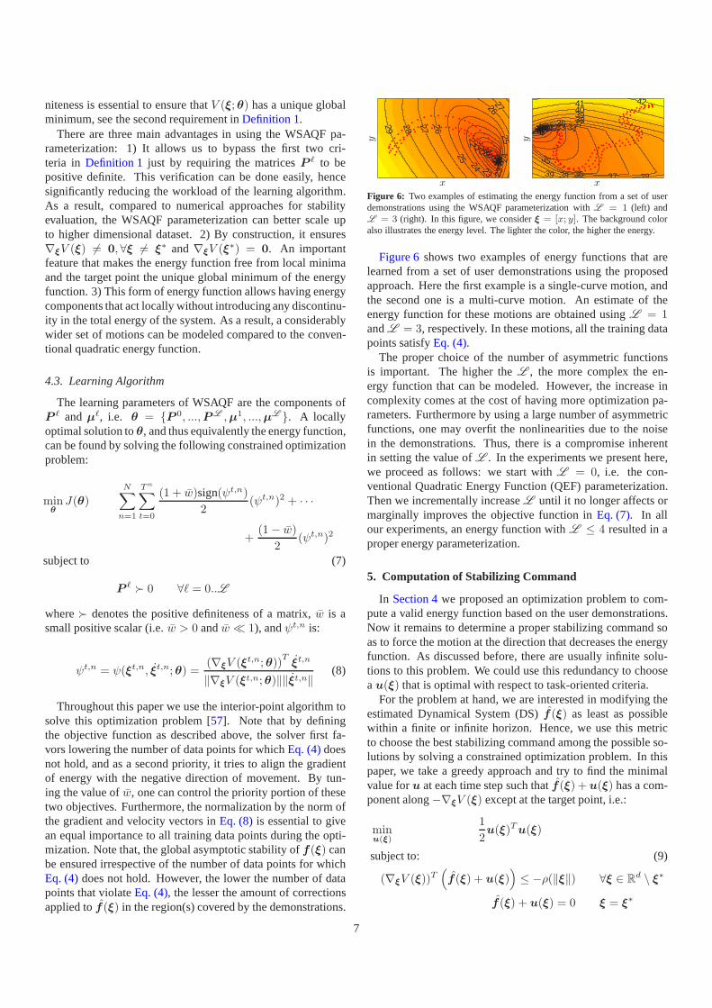
Figure 6: Two examples of estimating the energy function from a set of userdemonstrations using the WSAQF parameterization withL = 1 (left) andL = 3 (right). In this figure, we considerξ = [x; y]. The background coloralso illustrates the energy level. The lighter the color, the higher the energy.

Figure 6shows two examples of energy functions that arelearned from a set of user demonstrations using the proposedapproach. Here the first example is a single-curve motion, andthe second one is a multi-curve motion. An estimate of theenergy function for these motions are obtained usingL = 1andL = 3, respectively. In these motions, all the training datapoints satisfyEq. (4).

The proper choice of the number of asymmetric functionsis important. The higher theL , the more complex the en-ergy function that can be modeled. However, the increase incomplexity comes at the cost of having more optimization pa-rameters. Furthermore by using a large number of asymmetricfunctions, one may overfit the nonlinearities due to the noisein the demonstrations. Thus, there is a compromise inherentin setting the value ofL . In the experiments we present here,we proceed as follows: we start withL = 0, i.e. the con-ventional Quadratic Energy Function (QEF) parameterization.Then we incrementally increaseL until it no longer affects ormarginally improves the objective function inEq. (7). In allour experiments, an energy function withL ≤ 4 resulted in aproper energy parameterization.

5. Computation of Stabilizing Command

In Section 4we proposed an optimization problem to com-pute a valid energy function based on the user demonstrations.Now it remains to determine a proper stabilizing command soas to force the motion at the direction that decreases the energyfunction. As discussed before, there are usually infinite solu-tions to this problem. We could use this redundancy to chooseau(ξ) that is optimal with respect to task-oriented criteria.

For the problem at hand, we are interested in modifying theestimated Dynamical System (DS)f (ξ) as least as possiblewithin a finite or infinite horizon. Hence, we use this metricto choose the best stabilizing command among the possible so-lutions by solving a constrained optimization problem. In thispaper, we take a greedy approach and try to find the minimalvalue foru at each time step such thatf(ξ) +u(ξ) has a com-ponent along−∇ξV (ξ) except at the target point, i.e.:

minu(ξ)

1

2u(ξ)Tu(ξ)

subject to: (9)

(∇ξV (ξ))T(

f(ξ) + u(ξ))

≤ −ρ(‖ξ‖) ∀ξ ∈ Rd \ ξ∗

f(ξ) + u(ξ) = 0 ξ = ξ∗

7

ξ1

ξ2

91011

11

12

12

13

13

13

14

14

14

14

15

15

15

15

16 16

1616

17

17

17

17

18

18

18

19

19

2020

0

50

100

150

200

250

300

350

>400

Figure 7: Applyingu∗(ξ) from Eq. (10)to ensure global asymptotic stabilityof f(ξ) for the 2D toy example ofFig. 5. The value of1

2u∗(ξ)Tu∗(ξ) is

indicated with color gradient (unit ismm2/s2).

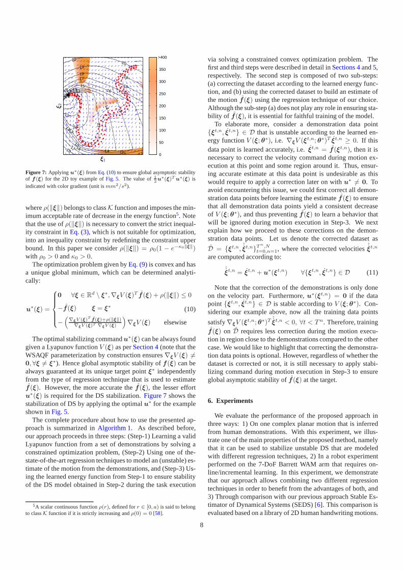
whereρ(‖ξ‖) belongs to classK function and imposes the min-imum acceptable rate of decrease in the energy function5. Notethat the use ofρ(‖ξ‖) is necessary to convert the strict inequal-ity constraint inEq. (3), which is not suitable for optimization,into an inequality constraint by redefining the constraint upperbound. In this paper we considerρ(‖ξ‖) = ρ0(1 − e−κ0‖ξ‖)with ρ0 > 0 andκ0 > 0.

The optimization problem given byEq. (9)is convex and hasa unique global minimum, which can be determined analyti-cally:

u∗(ξ) =

0 ∀ξ ∈ Rd \ ξ∗,∇ξV (ξ)T f (ξ) + ρ(‖ξ‖) ≤ 0

−f(ξ) ξ = ξ∗

−(

∇ξV (ξ)T f(ξ)+ρ(‖ξ‖)∇ξV (ξ)T ∇ξV (ξ)

)

∇ξV (ξ) elsewise

(10)

The optimal stabilizing commandu∗(ξ) can be always foundgiven a Lyapunov functionV (ξ) as perSection 4(note that theWSAQF parameterization by construction ensures∇ξV (ξ) 6=0, ∀ξ 6= ξ∗). Hence global asymptotic stability off(ξ) can bealways guaranteed at its unique target pointξ∗ independentlyfrom the type of regression technique that is used to estimatef (ξ). However, the more accurate thef(ξ), the lesser effortu∗(ξ) is required for the DS stabilization.Figure 7shows thestabilization of DS by applying the optimalu∗ for the exampleshown inFig. 5.

The complete procedure about how to use the presented ap-proach is summarized inAlgorithm 1. As described before,our approach proceeds in three steps: (Step-1) Learning a validLyapunov function from a set of demonstrations by solving aconstrained optimization problem, (Step-2) Using one of the-state-of-the-art regression techniques to model an (unstable) es-timate of the motion from the demonstrations, and (Step-3) Us-ing the learned energy function from Step-1 to ensure stabilityof the DS model obtained in Step-2 during the task execution

5A scalar continuous functionρ(r), defined forr ∈ [0, a) is said to belongto classK function if it is strictly increasing andρ(0) = 0 [58].

via solving a constrained convex optimization problem. Thefirst and third steps were described in detail inSections 4and5,respectively. The second step is composed of two sub-steps:(a) correcting the dataset according to the learned energy func-tion, and (b) using the corrected dataset to build an estimate ofthe motionf(ξ) using the regression technique of our choice.Although the sub-step (a) does not play any role in ensuring sta-bility of f(ξ), it is essential for faithful training of the model.

To elaborate more, consider a demonstration data point{ξt,n, ξt,n} ∈ D that is unstable according to the learned en-ergy functionV (ξ; θ∗), i.e. ∇ξV (ξt,n; θ∗)T ξt,n ≥ 0. If thisdata point is learned accurately, i.e.ξt,n = f(ξt,n), then it isnecessary to correct the velocity command during motion ex-ecution at this point and some region around it. Thus, ensur-ing accurate estimate at this data point is undesirable as thiswould require to apply a correction later on withu∗ 6= 0. Toavoid encountering this issue, we could first correct all demon-stration data points before learning the estimatef (ξ) to ensurethat all demonstration data points yield a consistent decreaseof V (ξ; θ∗), and thus preventingf(ξ) to learn a behavior thatwill be ignored during motion execution in Step-3. We nextexplain how we proceed to these corrections on the demon-stration data points. Let us denote the corrected dataset as

D = {ξt,n, ˆξt,n}Tn,N

t=0,n=1, where the corrected velocitiesξt,n

are computed according to:

ˆξt,n = ξt,n + u∗(ξt,n) ∀{ξt,n, ξt,n} ∈ D (11)

Note that the correction of the demonstrations is only doneon the velocity part. Furthermore,u∗(ξt,n) = 0 if the datapoint {ξt,n, ξt,n} ∈ D is stable according toV (ξ; θ∗). Con-sidering our example above, now all the training data points

satisfy∇ξV (ξt,n; θ∗)Tˆξt,n < 0, ∀t < T n. Therefore, training

f(ξ) on D requires less correction during the motion execu-tion in region close to the demonstrations compared to the othercase. We would like to highlight that correcting the demonstra-tion data points is optional. However, regardless of whether thedataset is corrected or not, it is still necessary to apply stabi-lizing command during motion execution in Step-3 to ensureglobal asymptotic stability off(ξ) at the target.

6. Experiments

We evaluate the performance of the proposed approach inthree ways: 1) On one complex planar motion that is inferredfrom human demonstrations. With this experiment, we illus-trate one of the main properties of the proposed method, namelythat it can be used to stabilize unstable DS that are modeledwith different regression techniques, 2) In a robot experimentperformed on the 7-DoF Barrett WAM arm that requires on-line/incremental learning. In this experiment, we demonstratethat our approach allows combining two different regressiontechniques in order to benefit from the advantages of both, and3) Through comparison with our previous approach Stable Es-timator of Dynamical Systems (SEDS) [6]. This comparison isevaluated based on a library of 2D human handwriting motions.

8

Algorithm 1 Control Lyapunov Function-based DynamicMovements (CLF-DM)

Step-1: Learning the Lyapunov Function:Input: D = {ξt,n, ξt,n}T

n,N

t=0,n=1 and a threshold valueκ1: L ← 02: i← 03: while truedo4: EstimateV (ξ;θi) by solvingEq. (7).5: if i > 0 and ‖J(θi)− J(θi−1)‖ < κ then6: break7: end if8: L ← L+ 19: end while

10: θ∗ ← θi−1

Output: V (ξ;θ∗)

Step-2: Learning the (unstable) DS Model:Input: D = {ξt,n, ξt,n}T

n,Nt=0,n=1 andV (ξ;θ∗)

11: (Optional): CorrectD based onV (ξ;θ∗) usingEq. (11)and saveit asD.

12: Learnf (ξ) from D using a regression method.Output: f(ξ)

Step-3: Robot Execution:Input: f(ξ), V (ξ;θ∗), ρ(‖ξ‖), initial stateξ0, target stateξ∗, accu-

racy toleranceǫ, and integration time stepδt13: i← 014: while ‖ξi − ξ∗‖ > ǫ do15: Computef(ξi)16: Computeu∗(ξi) from Eq. (10)17: ξi ← f (ξi) + u∗(ξi)18: Compute next stateξi+1 ← ξi + ξiδt

19: i← i+ 120: end while

6.1. Learning a Complex Motion with four Regression Methods

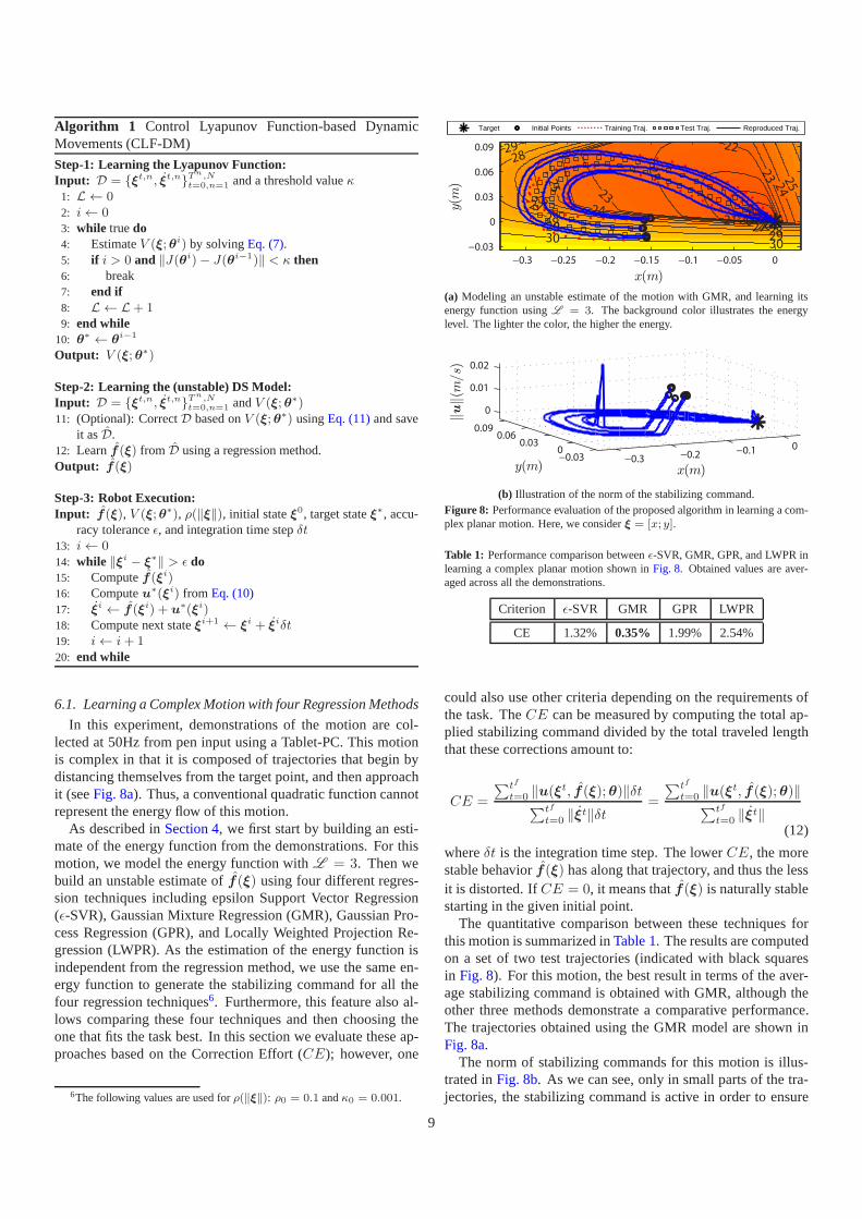
In this experiment, demonstrations of the motion are col-lected at 50Hz from pen input using a Tablet-PC. This motionis complex in that it is composed of trajectories that begin bydistancing themselves from the target point, and then approachit (seeFig. 8a). Thus, a conventional quadratic function cannotrepresent the energy flow of this motion.

As described inSection 4, we first start by building an esti-mate of the energy function from the demonstrations. For thismotion, we model the energy function withL = 3. Then webuild an unstable estimate off(ξ) using four different regres-sion techniques including epsilon Support Vector Regression(ǫ-SVR), Gaussian Mixture Regression (GMR), Gaussian Pro-cess Regression (GPR), and Locally Weighted Projection Re-gression (LWPR). As the estimation of the energy function isindependent from the regression method, we use the same en-ergy function to generate the stabilizing command for all thefour regression techniques6. Furthermore, this feature also al-lows comparing these four techniques and then choosing theone that fits the task best. In this section we evaluate these ap-proaches based on the Correction Effort (CE); however, one

6The following values are used forρ(‖ξ‖): ρ0 = 0.1 andκ0 = 0.001.

Target Initial Points Training Traj. Test Traj. Reproduced Traj.

−0.3 −0.25 −0.2 −0.15 −0.1 −0.05 0

−0.03

0

0.03

0.06

0.09

19202122

22

23

23

24

24

25

25

25

26

26

27

27

28

28

28

29

29293030

x(m)

y(m

)

(a) Modeling an unstable estimate of the motion with GMR, and learning itsenergy function usingL = 3. The background color illustrates the energylevel. The lighter the color, the higher the energy.

−0.3−0.2

−0.10

−0.030

0.030.06

0.09

0

0.01

0.02

x(m)y(m)kuk(m

/s)

(b) Illustration of the norm of the stabilizing command.Figure 8: Performance evaluation of the proposed algorithm in learning a com-plex planar motion. Here, we considerξ = [x;y].

Table 1: Performance comparison betweenǫ-SVR, GMR, GPR, and LWPR inlearning a complex planar motion shown inFig. 8. Obtained values are aver-aged across all the demonstrations.

Criterion ǫ-SVR GMR GPR LWPR

CE 1.32% 0.35% 1.99% 2.54%

could also use other criteria depending on the requirements ofthe task. TheCE can be measured by computing the total ap-plied stabilizing command divided by the total traveled lengththat these corrections amount to:

CE =

∑tf

t=0 ‖u(ξt, f (ξ); θ)‖δt

∑tf

t=0 ‖ξt‖δt

=

∑tf

t=0 ‖u(ξt, f (ξ); θ)‖

∑tf

t=0 ‖ξt‖

(12)

whereδt is the integration time step. The lowerCE, the morestable behaviorf(ξ) has along that trajectory, and thus the lessit is distorted. IfCE = 0, it means thatf(ξ) is naturally stablestarting in the given initial point.

The quantitative comparison between these techniques forthis motion is summarized inTable 1. The results are computedon a set of two test trajectories (indicated with black squaresin Fig. 8). For this motion, the best result in terms of the aver-age stabilizing command is obtained with GMR, although theother three methods demonstrate a comparative performance.The trajectories obtained using the GMR model are shown inFig. 8a.

The norm of stabilizing commands for this motion is illus-trated inFig. 8b. As we can see, only in small parts of the tra-jectories, the stabilizing command is active in order to ensure

9

convergence to the target. On average for the GMR model, thevalue of the correction effort is0.35%. Furthermore, the acti-vation of the stabilizing command on a small region around thetarget verifies thatf (ξ) is unstable, and without using the pre-sented approach, all trajectories would have missed the target.Finally, one can observe that the generated trajectories resem-ble the user demonstrations despite applying stabilizing com-mands. This is mainly due to the fact that stabilizing commandsare derived from an energy function that is estimated based onthe user demonstrations. Note that the result from this exper-iment does not necessarily imply that GMR outperforms otherregression techniques for any kind of motions. Instead, it aimsat providing a simple means to choose the best regression tech-nique for the task at hand.

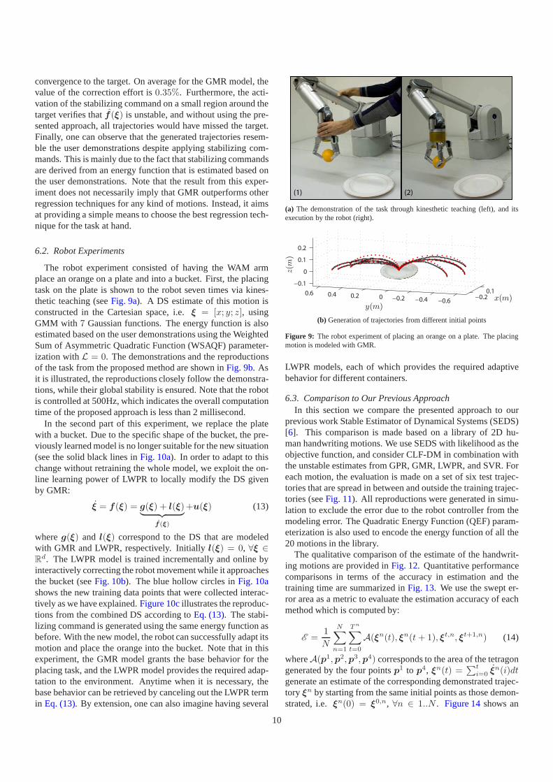
6.2. Robot Experiments

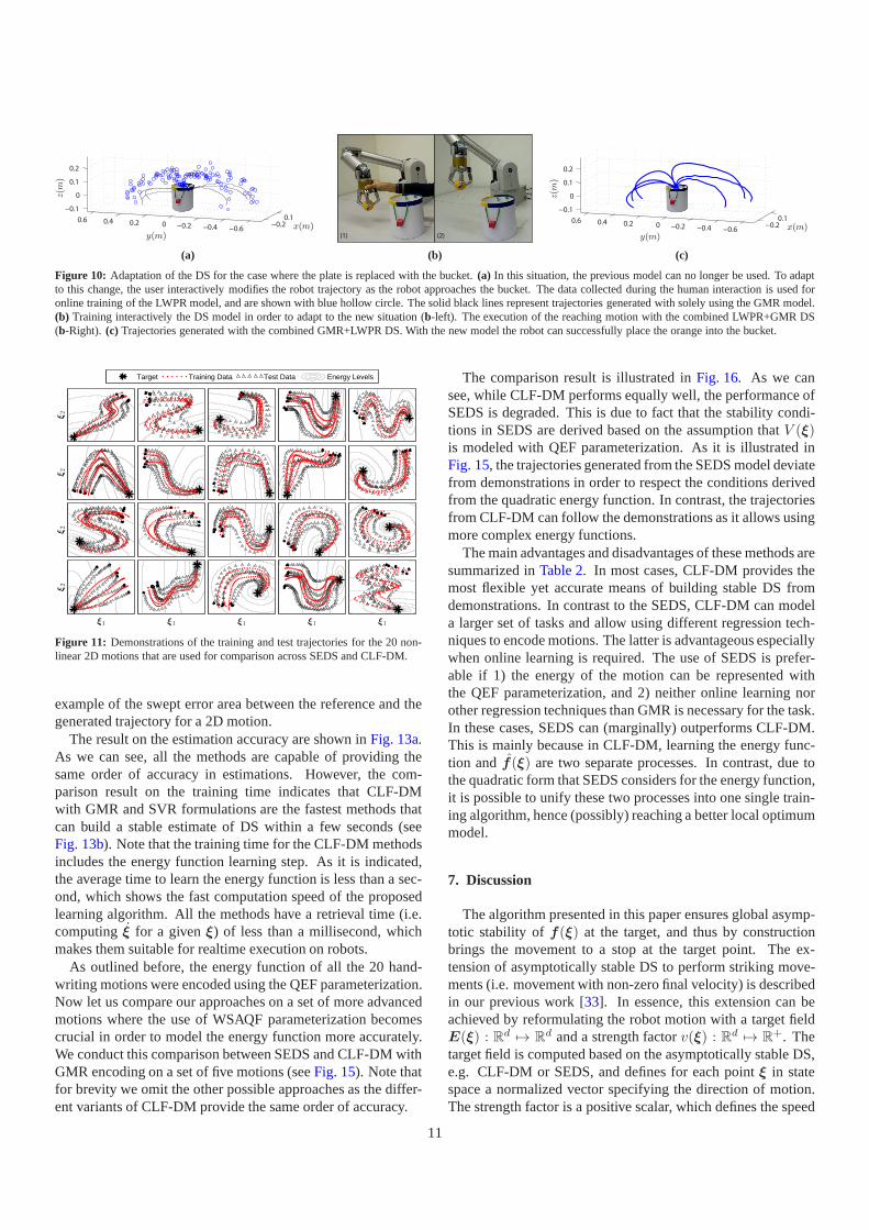
The robot experiment consisted of having the WAM armplace an orange on a plate and into a bucket. First, the placingtask on the plate is shown to the robot seven times via kines-thetic teaching (seeFig. 9a). A DS estimate of this motion isconstructed in the Cartesian space, i.e.ξ = [x; y; z], usingGMM with 7 Gaussian functions. The energy function is alsoestimated based on the user demonstrations using the WeightedSum of Asymmetric Quadratic Function (WSAQF) parameter-ization withL = 0. The demonstrations and the reproductionsof the task from the proposed method are shown inFig. 9b. Asit is illustrated, the reproductions closely follow the demonstra-tions, while their global stability is ensured. Note that the robotis controlled at 500Hz, which indicates the overall computationtime of the proposed approach is less than 2 millisecond.

In the second part of this experiment, we replace the platewith a bucket. Due to the specific shape of the bucket, the pre-viously learned model is no longer suitable for the new situation(see the solid black lines inFig. 10a). In order to adapt to thischange without retraining the whole model, we exploit the on-line learning power of LWPR to locally modify the DS givenby GMR:

ξ = f(ξ) = g(ξ) + l(ξ)︸ ︷︷ ︸

f(ξ)

+u(ξ) (13)

whereg(ξ) and l(ξ) correspond to the DS that are modeledwith GMR and LWPR, respectively. Initiallyl(ξ) = 0, ∀ξ ∈R

d. The LWPR model is trained incrementally and online byinteractively correcting the robot movement while it approachesthe bucket (seeFig. 10b). The blue hollow circles inFig. 10ashows the new training data points that were collected interac-tively as we have explained.Figure 10cillustrates the reproduc-tions from the combined DS according toEq. (13). The stabi-lizing command is generated using the same energy function asbefore. With the new model, the robot can successfully adapt itsmotion and place the orange into the bucket. Note that in thisexperiment, the GMR model grants the base behavior for theplacing task, and the LWPR model provides the required adap-tation to the environment. Anytime when it is necessary, thebase behavior can be retrieved by canceling out the LWPR termin Eq. (13). By extension, one can also imagine having several

(1) (2)

(a) The demonstration of the task through kinesthetic teaching (left), and itsexecution by the robot (right).

−0.20.1

−0.6−0.4−0.200.20.40.6

−0.1

0

0.1

0.2

x(m)y(m)

z(m

)

(b) Generation of trajectories from different initial points

Figure 9: The robot experiment of placing an orange on a plate. The placingmotion is modeled with GMR.

LWPR models, each of which provides the required adaptivebehavior for different containers.

6.3. Comparison to Our Previous ApproachIn this section we compare the presented approach to our

previous work Stable Estimator of Dynamical Systems (SEDS)[6]. This comparison is made based on a library of 2D hu-man handwriting motions. We use SEDS with likelihood as theobjective function, and consider CLF-DM in combination withthe unstable estimates from GPR, GMR, LWPR, and SVR. Foreach motion, the evaluation is made on a set of six test trajec-tories that are spread in between and outside the training trajec-tories (seeFig. 11). All reproductions were generated in simu-lation to exclude the error due to the robot controller from themodeling error. The Quadratic Energy Function (QEF) param-eterization is also used to encode the energy function of all the20 motions in the library.

The qualitative comparison of the estimate of the handwrit-ing motions are provided inFig. 12. Quantitative performancecomparisons in terms of the accuracy in estimation and thetraining time are summarized inFig. 13. We use the swept er-ror area as a metric to evaluate the estimation accuracy of eachmethod which is computed by:

E =1

N

N∑

n=1

Tn

∑

t=0

A(ξn(t), ξn(t+ 1), ξt,n, ξt+1,n) (14)

whereA(p1,p2,p3,p4) corresponds to the area of the tetragongenerated by the four pointsp1 to p4, ξn(t) =

∑t

i=0 ξn(i)dt

generate an estimate of the corresponding demonstrated trajec-tory ξn by starting from the same initial points as those demon-strated, i.e.ξn(0) = ξ0,n, ∀n ∈ 1..N . Figure 14shows an

10

−0.20.1

−0.6−0.4−0.200.20.40.6

−0.1

0

0.1

0.2

x(m)y(m)

z(m

)

(a)

(1) (2)

(b)

−0.20.1

−0.6−0.4−0.200.20.40.6

−0.1

0

0.1

0.2

x(m)y(m)

z(m

)

(c)

Figure 10: Adaptation of the DS for the case where the plate is replaced with the bucket.(a) In this situation, the previous model can no longer be used. To adaptto this change, the user interactively modifies the robot trajectory as the robot approaches the bucket. The data collected during the human interaction is used foronline training of the LWPR model, and are shown with blue hollow circle. The solid black lines represent trajectories generated with solely using the GMR model.(b) Training interactively the DS model in order to adapt to the new situation (b-left). The execution of the reaching motion with the combined LWPR+GMR DS(b-Right). (c) Trajectories generated with the combined GMR+LWPR DS. With the new model the robot can successfully place the orange into the bucket.

Target Training Data Test Data Energy Levels

ξ2

ξ1

ξ2

ξ1 ξ1 ξ1 ξ1

ξ1

ξ2

ξ1 ξ1 ξ1 ξ1

ξ1

ξ2

ξ1 ξ1 ξ1 ξ1

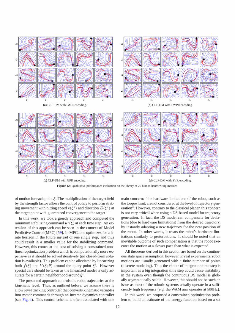
Figure 11: Demonstrations of the training and test trajectories for the 20 non-linear 2D motions that are used for comparison across SEDS and CLF-DM.

example of the swept error area between the reference and thegenerated trajectory for a 2D motion.

The result on the estimation accuracy are shown inFig. 13a.As we can see, all the methods are capable of providing thesame order of accuracy in estimations. However, the com-parison result on the training time indicates that CLF-DMwith GMR and SVR formulations are the fastest methods thatcan build a stable estimate of DS within a few seconds (seeFig. 13b). Note that the training time for the CLF-DM methodsincludes the energy function learning step. As it is indicated,the average time to learn the energy function is less than a sec-ond, which shows the fast computation speed of the proposedlearning algorithm. All the methods have a retrieval time (i.e.computingξ for a givenξ) of less than a millisecond, whichmakes them suitable for realtime execution on robots.

As outlined before, the energy function of all the 20 hand-writing motions were encoded using the QEF parameterization.Now let us compare our approaches on a set of more advancedmotions where the use of WSAQF parameterization becomescrucial in order to model the energy function more accurately.We conduct this comparison between SEDS and CLF-DM withGMR encoding on a set of five motions (seeFig. 15). Note thatfor brevity we omit the other possible approaches as the differ-ent variants of CLF-DM provide the same order of accuracy.

The comparison result is illustrated inFig. 16. As we cansee, while CLF-DM performs equally well, the performance ofSEDS is degraded. This is due to fact that the stability condi-tions in SEDS are derived based on the assumption thatV (ξ)is modeled with QEF parameterization. As it is illustrated inFig. 15, the trajectories generated from the SEDS model deviatefrom demonstrations in order to respect the conditions derivedfrom the quadratic energy function. In contrast, the trajectoriesfrom CLF-DM can follow the demonstrations as it allows usingmore complex energy functions.

The main advantages and disadvantages of these methods aresummarized inTable 2. In most cases, CLF-DM provides themost flexible yet accurate means of building stable DS fromdemonstrations. In contrast to the SEDS, CLF-DM can modela larger set of tasks and allow using different regression tech-niques to encode motions. The latter is advantageous especiallywhen online learning is required. The use of SEDS is prefer-able if 1) the energy of the motion can be represented withthe QEF parameterization, and 2) neither online learning norother regression techniques than GMR is necessary for the task.In these cases, SEDS can (marginally) outperforms CLF-DM.This is mainly because in CLF-DM, learning the energy func-tion andf(ξ) are two separate processes. In contrast, due tothe quadratic form that SEDS considers for the energy function,it is possible to unify these two processes into one single train-ing algorithm, hence (possibly) reaching a better local optimummodel.

7. Discussion

The algorithm presented in this paper ensures global asymp-totic stability of f(ξ) at the target, and thus by constructionbrings the movement to a stop at the target point. The ex-tension of asymptotically stable DS to perform striking move-ments (i.e. movement with non-zero final velocity) is describedin our previous work [33]. In essence, this extension can beachieved by reformulating the robot motion with a target fieldE(ξ) : Rd 7→ R

d and a strength factorv(ξ) : Rd 7→ R+. The

target field is computed based on the asymptotically stable DS,e.g. CLF-DM or SEDS, and defines for each pointξ in statespace a normalized vector specifying the direction of motion.The strength factor is a positive scalar, which defines the speed

11

ξ2

ξ1

ξ2

ξ1 ξ1 ξ1 ξ1

ξ1

ξ2

ξ1 ξ1 ξ1 ξ1

ξ1

ξ2

ξ1 ξ1 ξ1 ξ1

(a) CLF-DM with GMR encoding.

ξ2

ξ1

ξ2

ξ1 ξ1 ξ1 ξ1

ξ1

ξ2

ξ1 ξ1 ξ1 ξ1

ξ1

ξ2

ξ1 ξ1 ξ1 ξ1

(b) CLF-DM with LWPR encoding.

ξ2

ξ1

ξ2

ξ1 ξ1 ξ1 ξ1

ξ1

ξ2

ξ1 ξ1 ξ1 ξ1

ξ1

ξ2

ξ1 ξ1 ξ1 ξ1

(c) CLF-DM with GPR encoding.

ξ2

ξ1

ξ2

ξ1 ξ1 ξ1 ξ1

ξ1

ξ2

ξ1 ξ1 ξ1 ξ1

ξ1

ξ2

ξ1 ξ1 ξ1 ξ1

(d) CLF-DM with SVR encoding.

Figure 12: Qualitative performance evaluation on the library of 20 human handwriting motions.

of motion for each pointξ. The multiplication of the target fieldby the strength factor allows the control policy to perform strik-ing movement with hitting speedv(ξ∗) and directionE(ξ∗) atthe target point with guaranteed convergence to the target.

In this work, we took a greedy approach and computed theminimum stabilizing commandu∗(ξ) at each time step. An ex-tension of this approach can be seen in the context of ModelPredictive Control (MPC) [59]. In MPC, one optimizes for a fi-nite horizon in the future instead of one single step, and thuscould result in a smaller value for the stabilizing command.However, this comes at the cost of solving a constrained non-linear optimization problem which is computationally more ex-pensive as it should be solved iteratively (no closed-form solu-tion is available). This problem can be alleviated by linearizingboth f(ξ) andV (ξ; θ) around the query pointξt. Howeverspecial care should be taken as the linearized model is only ac-curate for a certain neighborhood aroundξt.

The presented approach controls the robot trajectories at thekinematic level. Thus, as outlined before, we assume there isa low level tracking controller that converts kinematic variablesinto motor commands through an inverse dynamics controller(seeFig. 4). This control scheme is often associated with one

main concern: “the hardware limitations of the robot, such asthe torque limit, are not considered at the level of trajectory gen-eration”. However, contrary to the classical planer, this concernis not very critical when using a DS-based model for trajectorygeneration. In fact, the DS model can compensate for devia-tions (due to hardware limitations) from the desired trajectory,by instantly adapting a new trajectory for the new position ofthe robot. In other words, it treats the robot’s hardware lim-itations similarly to perturbations. It should be noted that aninevitable outcome of such compensation is that the robot exe-cutes the motion at a slower pace than what is expected.

All theorems derived in this section are based on the continu-ous state space assumption; however, in real experiments, robotmotions are usually generated with a finite number of points(discrete modeling). Thus the choice of integration time step isimportant as a big integration time step could cause instabilityin the system even though the continuous DS model is glob-ally asymptotically stable. However, this should not be such anissue as most of the robotic systems usually operate in a suffi-ciently high frequency (e.g. the WAM arm operates at500Hz).

In this work, we proposed a constrained optimization prob-lem to build an estimate of the energy function based on a set

12

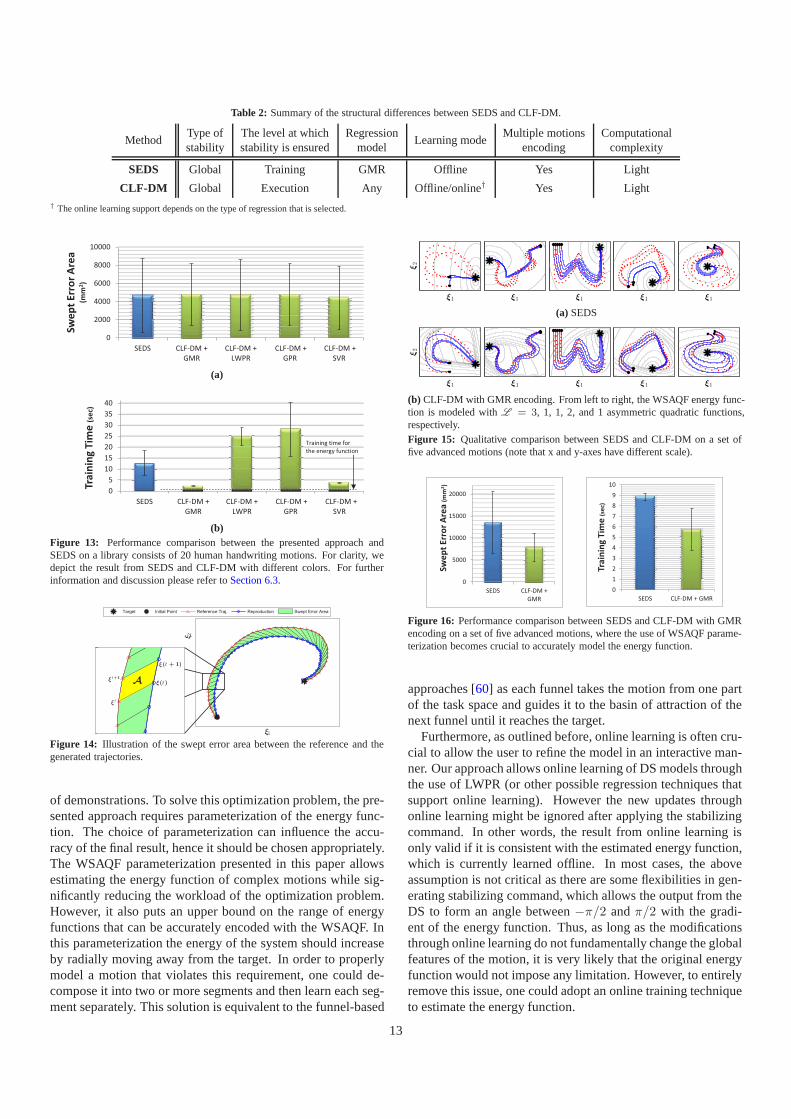
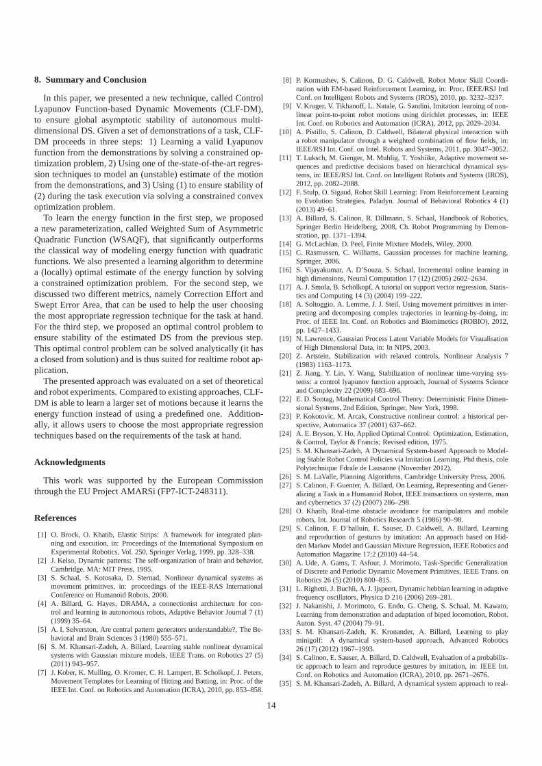
Table 2: Summary of the structural differences between SEDS and CLF-DM.

MethodType of The level at which Regression

Learning modeMultiple motions Computational

stability stability is ensured model encoding complexity

SEDS Global Training GMR Offline Yes Light

CLF-DM Global Execution Any Offline/online† Yes Light† The online learning support depends on the type of regression that is selected.

0

2000

4000

6000

8000

10000

SEDS CLF-DM +

GMR

CLF-DM +

LWPR

CLF-DM +

GPR

CLF-DM +

SVR

Sw

ep

t E

rro

r A

rea

(m

m2)

(a)

0

5

10

15

20

25

30

35

40

SEDS CLF-DM +

GMR

CLF-DM +

LWPR

CLF-DM +

GPR

CLF-DM +

SVR

Tra

inin

g T

ime

(se

c)

Training time for

the energy function

(b)Figure 13: Performance comparison between the presented approach andSEDS on a library consists of 20 human handwriting motions. For clarity, wedepict the result from SEDS and CLF-DM with different colors. For furtherinformation and discussion please refer toSection 6.3.

ξ1

ξ 2

ξ(t + 1)

ξ(t)

ξ t

ξ t+1

A

Figure 14: Illustration of the swept error area between the reference and thegenerated trajectories.

of demonstrations. To solve this optimization problem, the pre-sented approach requires parameterization of the energy func-tion. The choice of parameterization can influence the accu-racy of the final result, hence it should be chosen appropriately.The WSAQF parameterization presented in this paper allowsestimating the energy function of complex motions while sig-nificantly reducing the workload of the optimization problem.However, it also puts an upper bound on the range of energyfunctions that can be accurately encoded with the WSAQF. Inthis parameterization the energy of the system should increaseby radially moving away from the target. In order to properlymodel a motion that violates this requirement, one could de-compose it into two or more segments and then learn each seg-ment separately. This solution is equivalent to the funnel-based

ξ1

ξ2

ξ1 ξ1 ξ1 ξ1

(a) SEDS

ξ1

ξ2

ξ1 ξ1 ξ1 ξ1

(b) CLF-DM with GMR encoding. From left to right, the WSAQF energy func-tion is modeled withL = 3, 1, 1, 2, and 1 asymmetric quadratic functions,respectively.Figure 15: Qualitative comparison between SEDS and CLF-DM on a set offive advanced motions (note that x and y-axes have different scale).

0

5000

10000

15000

20000

SEDS CLF-DM +

GMR

Sw

ep

t E

rro

r A

rea

(m

m2)

0

1

2

3

4

5

6

7

8

9

10

SEDS CLF-DM + GMRTra

inin

g T

ime

(se

c)

Figure 16: Performance comparison between SEDS and CLF-DM with GMRencoding on a set of five advanced motions, where the use of WSAQF parame-terization becomes crucial to accurately model the energy function.

approaches [60] as each funnel takes the motion from one partof the task space and guides it to the basin of attraction of thenext funnel until it reaches the target.

Furthermore, as outlined before, online learning is often cru-cial to allow the user to refine the model in an interactive man-ner. Our approach allows online learning of DS models throughthe use of LWPR (or other possible regression techniques thatsupport online learning). However the new updates throughonline learning might be ignored after applying the stabilizingcommand. In other words, the result from online learning isonly valid if it is consistent with the estimated energy function,which is currently learned offline. In most cases, the aboveassumption is not critical as there are some flexibilities in gen-erating stabilizing command, which allows the output from theDS to form an angle between−π/2 andπ/2 with the gradi-ent of the energy function. Thus, as long as the modificationsthrough online learning do not fundamentally change the globalfeatures of the motion, it is very likely that the original energyfunction would not impose any limitation. However, to entirelyremove this issue, one could adopt an online training techniqueto estimate the energy function.

13

8. Summary and Conclusion

In this paper, we presented a new technique, called ControlLyapunov Function-based Dynamic Movements (CLF-DM),to ensure global asymptotic stability of autonomous multi-dimensional DS. Given a set of demonstrations of a task, CLF-DM proceeds in three steps: 1) Learning a valid Lyapunovfunction from the demonstrations by solving a constrained op-timization problem, 2) Using one of the-state-of-the-art regres-sion techniques to model an (unstable) estimate of the motionfrom the demonstrations, and 3) Using (1) to ensure stability of(2) during the task execution via solving a constrained convexoptimization problem.

To learn the energy function in the first step, we proposeda new parameterization, called Weighted Sum of AsymmetricQuadratic Function (WSAQF), that significantly outperformsthe classical way of modeling energy function with quadraticfunctions. We also presented a learning algorithm to determinea (locally) optimal estimate of the energy function by solvinga constrained optimization problem. For the second step, wediscussed two different metrics, namely Correction Effort andSwept Error Area, that can be used to help the user choosingthe most appropriate regression technique for the task at hand.For the third step, we proposed an optimal control problem toensure stability of the estimated DS from the previous step.This optimal control problem can be solved analytically (it hasa closed from solution) and is thus suited for realtime robot ap-plication.

The presented approach was evaluated on a set of theoreticaland robot experiments. Compared to existing approaches, CLF-DM is able to learn a larger set of motions because it learns theenergy function instead of using a predefined one. Addition-ally, it allows users to choose the most appropriate regressiontechniques based on the requirements of the task at hand.

Acknowledgments

This work was supported by the European Commissionthrough the EU Project AMARSi (FP7-ICT-248311).

References

[1] O. Brock, O. Khatib, Elastic Strips: A framework for integrated plan-ning and execution, in: Proceedings of the International Symposium onExperimental Robotics, Vol. 250, Springer Verlag, 1999, pp. 328–338.

[2] J. Kelso, Dynamic patterns: The self-organization of brain and behavior,Cambridge, MA: MIT Press, 1995.

[3] S. Schaal, S. Kotosaka, D. Sternad, Nonlinear dynamical systems asmovement primitives, in: proceedings of the IEEE-RAS InternationalConference on Humanoid Robots, 2000.

[4] A. Billard, G. Hayes, DRAMA, a connectionist architecture for con-trol and learning in autonomous robots, Adaptive Behavior Journal 7 (1)(1999) 35–64.

[5] A. I. Selverston, Are central pattern generators understandable?, The Be-havioral and Brain Sciences 3 (1980) 555–571.

[6] S. M. Khansari-Zadeh, A. Billard, Learning stable nonlinear dynamicalsystems with Gaussian mixture models, IEEE Trans. on Robotics 27 (5)(2011) 943–957.

[7] J. Kober, K. Mulling, O. Kromer, C. H. Lampert, B. Scholkopf, J. Peters,Movement Templates for Learning of Hitting and Batting, in: Proc. of theIEEE Int. Conf. on Robotics and Automation (ICRA), 2010, pp. 853–858.

[8] P. Kormushev, S. Calinon, D. G. Caldwell, Robot Motor Skill Coordi-nation with EM-based Reinforcement Learning, in: Proc. IEEE/RSJ IntlConf. on Intelligent Robots and Systems (IROS), 2010, pp. 3232–3237.

[9] V. Kruger, V. Tikhanoff, L. Natale, G. Sandini, Imitation learning of non-linear point-to-point robot motions using dirichlet processes, in: IEEEInt. Conf. on Robotics and Automation (ICRA), 2012, pp. 2029–2034.

[10] A. Pistillo, S. Calinon, D. Caldwell, Bilateral physical interaction witha robot manipulator through a weighted combination of flow fields, in:IEEE/RSJ Int. Conf. on Intel. Robots and Systems, 2011, pp. 3047–3052.

[11] T. Luksch, M. Gienger, M. Muhlig, T. Yoshiike, Adaptive movement se-quences and predictive decisions based on hierarchical dynamical sys-tems, in: IEEE/RSJ Int. Conf. on Intelligent Robots and Systems (IROS),2012, pp. 2082–2088.

[12] F. Stulp, O. Sigaud, Robot Skill Learning: From Reinforcement Learningto Evolution Strategies, Paladyn. Journal of Behavioral Robotics 4 (1)(2013) 49–61.

[13] A. Billard, S. Calinon, R. Dillmann, S. Schaal, Handbook of Robotics,Springer Berlin Heidelberg, 2008, Ch. Robot Programming by Demon-stration, pp. 1371–1394.

[14] G. McLachlan, D. Peel, Finite Mixture Models, Wiley, 2000.[15] C. Rasmussen, C. Williams, Gaussian processes for machine learning,

Springer, 2006.[16] S. Vijayakumar, A. D’Souza, S. Schaal, Incremental online learning in

high dimensions, Neural Computation 17 (12) (2005) 2602–2634.[17] A. J. Smola, B. Scholkopf, A tutorial on support vector regression, Statis-

tics and Computing 14 (3) (2004) 199–222.[18] A. Soltoggio, A. Lemme, J. J. Steil, Using movement primitives in inter-

preting and decomposing complex trajectories in learning-by-doing, in:Proc. of IEEE Int. Conf. on Robotics and Biomimetics (ROBIO), 2012,pp. 1427–1433.

[19] N. Lawrence, Gaussian Process Latent Variable Models for Visualisationof High Dimensional Data, in: In NIPS, 2003.

[20] Z. Artstein, Stabilization with relaxed controls, Nonlinear Analysis 7(1983) 1163–1173.

[21] Z. Jiang, Y. Lin, Y. Wang, Stabilization of nonlinear time-varying sys-tems: a control lyapunov function approach, Journal of Systems Scienceand Complexity 22 (2009) 683–696.

[22] E. D. Sontag, Mathematical Control Theory: Deterministic Finite Dimen-sional Systems, 2nd Edition, Springer, New York, 1998.

[23] P. Kokotovic, M. Arcak, Constructive nonlinear control: a historical per-spective, Automatica 37 (2001) 637–662.

[24] A. E. Bryson, Y. Ho, Applied Optimal Control: Optimization, Estimation,& Control, Taylor & Francis; Revised edition, 1975.

[25] S. M. Khansari-Zadeh, A Dynamical System-based Approach to Model-ing Stable Robot Control Policies via Imitation Learning, Phd thesis, colePolytechnique Fdrale de Lausanne (November 2012).

[26] S. M. LaValle, Planning Algorithms, Cambridge University Press, 2006.[27] S. Calinon, F. Guenter, A. Billard, On Learning, Representing and Gener-

alizing a Task in a Humanoid Robot, IEEE transactions on systems, manand cybernetics 37 (2) (2007) 286–298.

[28] O. Khatib, Real-time obstacle avoidance for manipulators and mobilerobots, Int. Journal of Robotics Research 5 (1986) 90–98.

[29] S. Calinon, F. D’halluin, E. Sauser, D. Caldwell, A. Billard, Learningand reproduction of gestures by imitation: An approach based on Hid-den Markov Model and Gaussian Mixture Regression, IEEE Robotics andAutomation Magazine 17:2 (2010) 44–54.

[30] A. Ude, A. Gams, T. Asfour, J. Morimoto, Task-Specific Generalizationof Discrete and Periodic Dynamic Movement Primitives, IEEE Trans. onRobotics 26 (5) (2010) 800–815.

[31] L. Righetti, J. Buchli, A. J. Ijspeert, Dynamic hebbian learning in adaptivefrequency oscillators, Physica D 216 (2006) 269–281.

[32] J. Nakanishi, J. Morimoto, G. Endo, G. Cheng, S. Schaal, M. Kawato,Learning from demonstration and adaptation of biped locomotion, Robot.Auton. Syst. 47 (2004) 79–91.

[33] S. M. Khansari-Zadeh, K. Kronander, A. Billard, Learning to playminigolf: A dynamical system-based approach, Advanced Robotics26 (17) (2012) 1967–1993.

[34] S. Calinon, E. Sauser, A. Billard, D. Caldwell, Evaluation of a probabilis-tic approach to learn and reproduce gestures by imitation, in: IEEE Int.Conf. on Robotics and Automation (ICRA), 2010, pp. 2671–2676.

[35] S. M. Khansari-Zadeh, A. Billard, A dynamical system approach to real-

14

time obstacle avoidance, Autonomous Robots 32 (2012) 433–454.[36] D.-H. Park, H. Hoffmann, P. Pastor, S. Schaal, Movement reproduction

and obstacle avoidance with dynamic movement primitives and potentialfields, in: IEEE Int. Conf. on Humanoid Robotics, 2008, pp. 91–98.

[37] F. Stulp, G. Raiola, A. Hoarau, S. Ivaldi, O. Sigaud, Learning CompactParameterized Skills with a Single Regression, in: Proc. IEEE-RAS Int.Conf. on Humanoid Robots (Humanoids), 2013, pp. 1–7.

[38] S. Schaal, A. J. Ijspeert, A. Billard, Computational Approaches to MotorLearning by Imitation, Philosophical Transactions: Biological Sciences(The Royal Society) 358 (1431) (2003) 537–547.

[39] D. Wolpert, M. Kawato, Multiple paired forward and inverse models formotor control, Neural Networks 11 (1998) 1317–1329.

[40] D. Bullock, S. Grossberg, The VITE Model: A Neural Command Cir-cuit for Generating Arm and Articulator Trajectories, Dynamic Patternsin Complex Systems (1988) 305–326.

[41] P. Gaudiano, S. Grossberg, Adaptive vector integration to endpoint: Self-organizing neural circuits for control of plannedmovement trajectories,Human Movement Science 11 (1992) 141–155.

[42] M. Raibert, Legged robots that balance, Cambridge MA: MIT Press,1986.

[43] A. J. Ijspeert, J. Hallam, D. Willshaw, Evolution of a central pattern gen-erator for the swimming and trotting gaits of the salamander, in: Int. Conf.on Computational Intelligence & Neurosciences (ICCIN), 1998, pp. 24–38.

[44] M. Lukosevicius, H. Jaeger, Reservoir computing approaches to recurrentneural network training, Computer Science Review 3 (3) (2009) 127–149.

[45] R. F. Reinhart, J. J. Steil, Neural learning and dynamical selection of re-dundant solutions for inverse kinematic control, in: IEEE-RAS Int. Conf.on Humanoid Robots (Humanoids), 2011, pp. 564–569.

[46] B. Pearlmutter, Learning state space trajectories in recurrent neural net-works, Neural Computation 1 (1989) 263–269.

[47] A. F. Atiya, A. G. Parlos, S. Member, S. Member, New Results on Recur-rent Network Training: Unifying the Algorithms and Accelerating Con-vergence, IEEE Trans. Neural Networks 11 (2000) 697–709.

[48] S. Schaal, Dynamic movement primitives - A framework for motor con-trol in humans and humanoid robots, in: Int. Symposium on AdaptiveMotion of Animals and Machines, 2003.

[49] B. Nemec, M. Tamosiunaite, F. Worgotter, A. Ude, Task adaptationthrough exploration and action sequencing, in: Proc. of the IEEE-RASInt. Conf. on Humanoid Robots (Humanoids), 2009, pp. 610–616.

[50] S. M. Khansari-Zadeh, A. Billard, BM: An iterative algorithm to learnstable non-linear dynamical systems with Gaussian mixture models, in:Int, Conf. on Robotics and Automation (ICRA), 2010, pp. 2381–2388.

[51] S. Calinon, A. Pistillo, D. G. Caldwell, Encoding the time and space con-straints of a task in explicit-duration hidden Markov model, in: Proc.IEEE/RSJ Int. Conf. on Intelligent Robots and Systems (IROS), 2011,pp. 3413–3418.

[52] K. Kronander, S. M. Khansari Zadeh, A. Billard, Learning to control pla-nar hitting motions in a minigolf-like task, in: Proc. of the IEEE/RSJ Int.Conf. on Intelligent Robots and Systems (IROS), 2011, pp. 710–717.

[53] A. Shukla, A. Billard, Coupled dynamical system based arm-hand grasp-ing model for learning fast adaptation strategies, Robotics and Au-tonomous Systems 60 (3) (2012) 424–440.

[54] K. Kronander, A. Billard, Learning compliant manipulation throughkinesthetic and tactile human-robot interaction, IEEE Transactions onHaptics.

[55] S. Kim, Rapid and reactive robot control framework for catching objectsin flight, Phd thesis, cole Polytechnique Fdrale de Lausanne (2014).

[56] A. Shukla, A. Billard, Augmented-SVM: Automatic space partitioningfor combining multiple non-linear dynamics, in: Advances in Neural In-formation Processing Systems (NIPS), 2012, pp. 1025–1033.

[57] J. Bonnans, J. Gilbert, Numerical Optimization, 2nd Edition, Springer,2006.

[58] H. Khalil, Nonlinear systems, Prentice Hall Upper Saddle River, 1996.[59] P. Kulchenko, E. Todorov, First-exit model predictive control of fast dis-

continuous dynamics: Application to ball bouncing, in: IEEE Int. Conf.on Robotics and Automation (ICRA), 2011, pp. 2144–2151.

[60] L. Yang, S. LaValle, The sampling-based neighborhood graph: an ap-proach to computing and executing feedback motion strategies, IEEETransactions on Robotics and Automation 20 (3) (2004) 419–432.

Seyed Mohammad Khansari-Zadeh is a post-doctoral researcher at LASA laboratory at EPFL. Hereceived his Ph.D. (2012) in Robotics from EPFL,and his M.Sc. (2008) in Dynamics and Control fromSharif University of Technology. His research inter-ests include imitation learning for robot control, dy-namical systems, nonlinear control, and humanoids.

Aude Billard is Associate Professor and head of theLearning Algorithms and Systems Laboratory at theSchool of Engineering at EPFL. She received herB.Sc. (1994) and M.Sc. (1995) in Physics from EPFLand her Ph.D. in Artificial Intelligence (1998) fromthe University of Edinburgh.

15