LYAPUNOV-BASED CONTROL OF SATURATED AND …ncr.mae.ufl.edu/dissertations/nic.pdf · lyapunov-based control of saturated and time-delayed nonlinear systems by nicholas fischer a dissertation

LYAPUNOV-BASED CONTROL OF SATURATED AND TIME-DELAYED NONLINEARSYSTEMS

By

NICHOLAS FISCHER

A DISSERTATION PRESENTED TO THE GRADUATE SCHOOLOF THE UNIVERSITY OF FLORIDA IN PARTIAL FULFILLMENT

OF THE REQUIREMENTS FOR THE DEGREE OFDOCTOR OF PHILOSOPHY

UNIVERSITY OF FLORIDA

2012

c© 2012 Nicholas Fischer

2

To my parents Debbie and Matt Fischer for their enduring support

and constant encouragement

3

ACKNOWLEDGMENTS

I would like to express sincere gratitude to my advisor, Dr. Warren E. Dixon, whose

experience and motivation have been instrumental in my academic success. As an

advisor, he has provided guidance in my research and encouragement in developing my

own ideas. As a mentor, he has helped me develop professional skills and has prepared

me for the future. I would like to extend my gratitude to my committee members Prabir

Barooah, Carl Crane, Pramod Khargonekar, and Eric. M. Schwartz for the time and

recommendations they provided. Also, I would like to thank my family, coworkers

(especially Rushikesh Kamalapurkar for his countless hours of coauthoring work with

nonsmooth analysis), and friends for their support and inspiritment.

4

TABLE OF CONTENTS

page

ACKNOWLEDGMENTS . . . . . . . . . . . . . . . . . . . . . . . . . . . . . . . . . . 4

LIST OF FIGURES . . . . . . . . . . . . . . . . . . . . . . . . . . . . . . . . . . . . . 7

LIST OF ABBREVIATIONS . . . . . . . . . . . . . . . . . . . . . . . . . . . . . . . . 8

ABSTRACT . . . . . . . . . . . . . . . . . . . . . . . . . . . . . . . . . . . . . . . . . 9

CHAPTER

1 INTRODUCTION . . . . . . . . . . . . . . . . . . . . . . . . . . . . . . . . . . . 11

1.1 Motivation and Problem Statement . . . . . . . . . . . . . . . . . . . . . . 111.2 Literature Review . . . . . . . . . . . . . . . . . . . . . . . . . . . . . . . . 151.3 Contributions . . . . . . . . . . . . . . . . . . . . . . . . . . . . . . . . . . 23

2 LASALLE-YOSHIZAWA COROLLARY FOR DISCONTINUOUS SYSTEMS . . 27

2.1 Preliminaries . . . . . . . . . . . . . . . . . . . . . . . . . . . . . . . . . . 272.2 Main Result . . . . . . . . . . . . . . . . . . . . . . . . . . . . . . . . . . . 322.3 Design Example 1 (Adaptive + Sliding Mode) . . . . . . . . . . . . . . . . 362.4 Design Example 2 (RISE) . . . . . . . . . . . . . . . . . . . . . . . . . . . 402.5 Summary . . . . . . . . . . . . . . . . . . . . . . . . . . . . . . . . . . . . 47

3 SATURATED RISE FEEDBACK CONTROL . . . . . . . . . . . . . . . . . . . . 48

3.1 Dynamic Model . . . . . . . . . . . . . . . . . . . . . . . . . . . . . . . . . 483.2 Control Development . . . . . . . . . . . . . . . . . . . . . . . . . . . . . . 493.3 Stability Analysis . . . . . . . . . . . . . . . . . . . . . . . . . . . . . . . . 533.4 Euler-Lagrange Extension . . . . . . . . . . . . . . . . . . . . . . . . . . . 573.5 Experimental Results . . . . . . . . . . . . . . . . . . . . . . . . . . . . . . 613.6 Summary . . . . . . . . . . . . . . . . . . . . . . . . . . . . . . . . . . . . 64

4 RISE-BASED CONTROL OF AN UNCERTAIN NONLINEAR SYSTEM WITHTIME-VARYING STATE DELAYS . . . . . . . . . . . . . . . . . . . . . . . . . . 65

4.1 Dynamic Model . . . . . . . . . . . . . . . . . . . . . . . . . . . . . . . . . 654.2 Control Development . . . . . . . . . . . . . . . . . . . . . . . . . . . . . . 664.3 Stability Analysis . . . . . . . . . . . . . . . . . . . . . . . . . . . . . . . . 714.4 Summary . . . . . . . . . . . . . . . . . . . . . . . . . . . . . . . . . . . . 75

5 LYAPUNOV-BASED CONTROL OF AN UNCERTAIN NONLINEAR SYSTEMWITH TIME-VARYING INPUT DELAY . . . . . . . . . . . . . . . . . . . . . . . 76

5.1 Dynamic Model . . . . . . . . . . . . . . . . . . . . . . . . . . . . . . . . . 765.2 Control Development . . . . . . . . . . . . . . . . . . . . . . . . . . . . . . 77

5

5.3 Stability Analysis . . . . . . . . . . . . . . . . . . . . . . . . . . . . . . . . 795.4 Euler-Lagrange Extension . . . . . . . . . . . . . . . . . . . . . . . . . . . 835.5 Simulation Results . . . . . . . . . . . . . . . . . . . . . . . . . . . . . . . 865.6 Summary . . . . . . . . . . . . . . . . . . . . . . . . . . . . . . . . . . . . 87

6 TIME-VARYING INPUT AND STATE DELAY COMPENSATION FOR UNCER-TAIN NONLINEAR SYSTEMS . . . . . . . . . . . . . . . . . . . . . . . . . . . 89

6.1 Dynamic Model . . . . . . . . . . . . . . . . . . . . . . . . . . . . . . . . . 896.2 Control Development . . . . . . . . . . . . . . . . . . . . . . . . . . . . . . 906.3 Stability Analysis . . . . . . . . . . . . . . . . . . . . . . . . . . . . . . . . 946.4 Simulation Results . . . . . . . . . . . . . . . . . . . . . . . . . . . . . . . 986.5 Summary . . . . . . . . . . . . . . . . . . . . . . . . . . . . . . . . . . . . 100

7 SATURATED CONTROL OF AN UNCERTAIN NONLINEAR SYSTEM WITHINPUT DELAY . . . . . . . . . . . . . . . . . . . . . . . . . . . . . . . . . . . . 103

7.1 Dynamic Model . . . . . . . . . . . . . . . . . . . . . . . . . . . . . . . . . 1037.2 Control Development . . . . . . . . . . . . . . . . . . . . . . . . . . . . . . 1047.3 Stability Analysis . . . . . . . . . . . . . . . . . . . . . . . . . . . . . . . . 1087.4 Euler-Lagrange Extension . . . . . . . . . . . . . . . . . . . . . . . . . . . 1127.5 Simulation Results . . . . . . . . . . . . . . . . . . . . . . . . . . . . . . . 1147.6 Summary . . . . . . . . . . . . . . . . . . . . . . . . . . . . . . . . . . . . 115

8 CONCLUSION AND FUTURE WORK . . . . . . . . . . . . . . . . . . . . . . . 118

8.1 Dissertation Summary . . . . . . . . . . . . . . . . . . . . . . . . . . . . . 1188.2 Limitations and Future Work . . . . . . . . . . . . . . . . . . . . . . . . . . 120

APPENDIX

A PROOF OF P (CH 3) . . . . . . . . . . . . . . . . . . . . . . . . . . . . . . . . 123

B PROOF OF P (CH 6) . . . . . . . . . . . . . . . . . . . . . . . . . . . . . . . . 125

C PROOF OF χ BOUND (CH 7) . . . . . . . . . . . . . . . . . . . . . . . . . . . . 127

REFERENCES . . . . . . . . . . . . . . . . . . . . . . . . . . . . . . . . . . . . . . . 130

BIOGRAPHICAL SKETCH . . . . . . . . . . . . . . . . . . . . . . . . . . . . . . . . 144

6

LIST OF FIGURES

Figure page

2-1 Set closure of K [f ] (x) for x > 0 case. . . . . . . . . . . . . . . . . . . . . . . . 30

2-2 Set closure of K [f ] (x) for x = 0 case. . . . . . . . . . . . . . . . . . . . . . . . 30

3-1 Tracking errors vs. time for controller proposed in (3–11). . . . . . . . . . . . . 63

3-2 Desired and actual trajectories vs. time for controller proposed in (3–11). . . . 63

3-3 Control torque vs. time for controller proposed in (3–11). . . . . . . . . . . . . . 64

5-1 Tracking errors vs. time for controller proposed in (5–6) with +50% frequencyvariance in input delay. . . . . . . . . . . . . . . . . . . . . . . . . . . . . . . . . 88

6-1 Tracking errors vs. time for the proposed controller in (6–12). . . . . . . . . . . 100

6-2 Tracking errors, actuation effort and time-varying delays vs time for Case 3. . . 101

6-3 Tracking errors, actuation effort and time-varying delays vs time for Case 5. . . 101

7-1 Tracking error vs. time for proposed controller in (7–10). . . . . . . . . . . . . . 116

7-2 Control torque vs. time for proposed controller in (7–10). . . . . . . . . . . . . . 116

7

LIST OF ABBREVIATIONS

a.e. Almost Everywhere

DCAL Desired Compensation Adaptation Law

EL Euler-Lagrange

EMK Exact Model Knowledge

LK Lyapunov-Krasovskii

LMI Linear Matrix Inequality

LP Linear-in-the-Parameters

LR Lyapunov-Razumikhin

LYC LaSalle-Yoshizawa Corollaries

LYT LaSalle-Yoshizawa Theorem

MVT Mean Value Theorem

NN Neural Network

non-LP Not Linear-in-the-Parameters

PD Proportional-Derivative

PID Proportional-Integral-Derivative

RHS Right-Hand Side

RISE Robust Integral of the Sign of the Error

RMS Root Mean Square

SARC Saturated Adaptive Robust Control

UC Uniformly Continuous

UUB Uniformly Ultimately Bounded

8

Abstract of Dissertation Presented to the Graduate Schoolof the University of Florida in Partial Fulfillment of theRequirements for the Degree of Doctor of Philosophy

LYAPUNOV-BASED CONTROL OF SATURATED AND TIME-DELAYED NONLINEARSYSTEMS

By

Nicholas Fischer

December 2012

Chair: Warren E. DixonMajor: Mechanical Engineering

Time delays and actuator saturation are two phenomena which affect the perfor-

mance of dynamic systems under closed-loop control. Effective compensation mech-

anisms can be applied to systems with actuator constraints or time delays in either the

state or the control. The focus of this dissertation is the design of control strategies for

nonlinear systems with combinations of parametric uncertainty, bounded disturbances,

actuator saturation, time delays in the state, and/or time delays in the input.

The first contribution of this work is the development of a saturated control strategy

based on the Robust Integral of the Sign of the Error (RISE), capable of compensating

for system uncertainties and bounded disturbances. To facilitate the design of this

controller and analysis, two Lyapunov-based stability corollaries based on the LaSalle-

Yoshizawa Theorem (LYT) are introduced using nonsmooth analysis techniques.

Leveraging these two results, a RISE-based control design for systems with time-

varying state-delays is developed. Since delays can also commonly occur in the control

input, a predictor-based control strategy for systems with time-varying input delays is

presented. Extending the results for time-delayed systems, a predictor-based controller

for uncertain nonlinear systems subject to simultaneous time-varying unknown state

and known input delays is introduced. Because errors can build over the deadtime

interval when input delays are present leading to large actuator demands, a predictor-

based saturated controller for uncertain nonlinear systems with constant input-delays

9

is developed. Each of the proposed controllers provides advantages over previous

literature in their ability to provide smooth, continuous control signals in the presence

of exogenous bounded disturbances. Lyapunov-based stability analyses, extensions

to Euler-Lagrange (EL) dynamic systems, simulations, and experiments are also

provided to demonstrate the performance of each of the control designs throughout the

dissertation.

10

CHAPTER 1INTRODUCTION

1.1 Motivation and Problem Statement

There exist numerous control solutions for nonlinear systems with additive distur-

bances. General control literature suggests that robust techniques (such as high gain,

sliding mode, or variable structure control) have successfully been developed to accom-

modate for parametric uncertainties and disturbances in nonlinear plants [1–7]. The

coupling of these robust methods with adaptive components has also been shown to

improve the overall performance of both regulation and tracking problems for nonlinear

systems. Robust control techniques that yield an asymptotic result are typically discon-

tinuous, and often suffer from limitations such as the demand for infinite bandwidth or

chatter. Continuous robust control designs such as the RISE strategy [8] have also been

developed and have been shown to be effective for systems with bounded disturbances.

The RISE strategy works by implicitly learning [9] and compensating for sufficiently

smooth bounded disturbances and unstructured parametric uncertainty through the use

of a sufficiently large gain multiplied by an integral signum term. RISE techniques are

used throughout the dissertation as they present a state-of-the-art approach for control

of uncertain nonlinear systems.

Classical stability theory is not applicable for systems described by discontinuous

differential equations based on the local Lipschitz assumption (i.e., nonsmooth sys-

tems). Examples of such systems include: systems with friction modeled as a force

proportional to the sign of a velocity, systems with feedback from a network, digital

systems, systems with a discontinuous control law, etc. Differential inclusions are a

mathematical tool that can be used to discuss the existence of solutions for nonsmooth

systems. Utilizing a differential inclusion framework, numerous Lyapunov methods using

generalized notions of solutions have been developed in literature for both autonomous

11

and nonautonomous systems. Of these, several stability theorems have been estab-

lished which apply to nonsmooth systems for which the derivative of the candidate

Lyapunov function can be upper bounded by a negative-definite function: Lyapunov’s

generalized theorem and finite-time convergence in [10–15] are some examples of such.

However, for certain classes of controllers (e.g., adaptive controllers, output feedback

controllers, etc.), a negative-definite bound may be difficult (or impossible) to achieve,

restricting the use of such methods.

Stability techniques such as the LaSalle-Yoshizawa Theorem (LYT) were introduced

for continuous systems to specifically handle the case when the Lyapunov function

derivative is bounded by a semi-definite function. Historically, some authors have stated

the use of the LYT incorrectly (if the system contains discontinuities, then the locally

Lipschitz property required by the theorem does not hold) or have stated that the LYT

can applied using nonsmooth techniques without proof. The focus of Chapter 2 is the

explicit development of a corollary to the LYT which can be used as an analysis tool for

nonsmooth systems with a negative-semi-definite derivative of the candidate Lyapunov

function.

While robust control techniques (whether continuous or discontinuous) have been

shown to be effective for the compensation of parametric uncertainties and additive

disturbances, in general, these techniques (including all previous RISE methods)

do not account for the fact that the commanded input may require more actuation

than is physically possible by the system (e.g., due to large initial condition offsets,

an aggressive desired trajectory, or large perturbations). For example, the typical

RISE structure uses a sufficiently large gain multiplied by an integral term, which can

potentially lead to a computed control command that exceeds actuator capabilities.

Because degraded control performance and the potential risk of thermal or mechanical

failure can occur when unmodeled actuator constraints are violated, control schemes

which can ensure performance while operating within actuator limitations are motivated.

12

Leveraging the outcomes developed in Chapter 2, Chapter 3 presents a saturated

RISE controller which limits the control authority at or below an adjustable a priori

limit. Saturated control designs are available in literature; however, the integration of a

saturation scheme into the continuous RISE structure has remained an open problem

due, in part to the integrator compensation.

As described in the survey papers [16–19] and relatively recent monographs such

as [20–25], time delays are pervasive in nature and engineered systems. A few well-

known and documented engineering applications include: digital implementation of a

continuous control signal, regenerative chatter in metal cutting (especially prevalent

in high speed manufacturing), delays in torque production due to engine cycle delays

in internal combustion engines, chemical process control, rolling mills, control over

networks, active queue management, financial markets (especially, computer controller

exchanges of financial products), etc. Delays are also inherent in many biological

process such as: delay in a person’s response due to drugs and alcohol, delays in

force production in muscle, the cardiovascular control system, etc. Systems that do not

compensate for delays can exhibit reduced performance and potential instability.

Since a time delay can be considered another type of disturbance to the system,

researchers have investigated adaptive and/or robust techniques to compensate for

the undesirable implications delays have on closed-loop control of nonlinear systems.

Typical time delayed control results have used novel prediction/compensation tech-

niques (such as Smith predictors or Artstein reduction methods) to handle the delayed

terms in closed-loop control; however, methods that achieve asymptotic or exponential

results utilizing classic robust techniques suffer from the same discontinuous limitations

(e.g., demand for infinite bandwidth and/or chatter) as delay-free control designs. Lever-

aging a design approach similar to that of the previous chapter, Chapter 4 presents a

RISE-based control design for nonlinear systems with time-varying state delays.

13

While state delays are prevalent in a number of engineered systems, time delays

can also occur in the control. Examples of systems with input delays can be found in

numerous applications, from teleoperated robotic systems to biological processes.

Problems arising from delay corruption of the control input remain unsolved for large

classes of practical systems (e.g., uncertain nonlinear systems). While several results

have used variations of the Smith and Artstein methods to solve the input delay problem

for linear systems (with known and unknown dynamics), and nonlinear systems with

exact model knowledge (EMK) (i.e., known forward-complete and strict feedforward

systems), few results solve the input delay problem for uncertain nonlinear systems.

As stated in the “Beyond this Book” section of the seminal work in [22], Krstic indicates

that approaches developed for uncertain linear systems do not extend in an obvious

way to nonlinear plants since the linear boundedness of the plant model is explicitly

used in the stability proof of such results, and that new methods must be developed

for delay-adaptive control for select classes of nonlinear systems with unknown input

delays. Methods that solve the input delay problem for uncertain nonlinear systems with

known and unknown constant time delays have been studied in [26–32]. However, due

to uncertainties in the inherent nature of real world systems, it is often more practical to

consider time-varying or state-dependent time delays in the control. Chapter 5 presents

a controller for uncertain nonlinear systems with time-varying input delays. Motivated by

the same time-varying delay considerations, Chapter 6 integrates the work of Chapters

2, 4 and 5 to design a controller which is capable of handling composite time-varying

state delays and time-varying input delays, while achieving better transient and steady

state performance and stability.

For systems with input delays, errors can build over the delay interval also leading

to large actuator demands, exacerbating potential problems with actuator saturation.

Motivated by the same actuator saturation concerns presented in Chapter 3, Chapter 7

develops a control strategy for uncertain input-delayed nonlinear systems with constant

14

time delays and actuator saturation constraints. Previous techniques and outcomes

obtained in Chapter 3 are utilized to develop a continuous control design which allows

for the bound on the control to be adjusted a priori.

The work in this dissertation is based on Lyapunov stability theory (a common

tool in nonlinear control) and presents several control strategies for open problems in

nonlinear control literature. Specifically, the work focuses on real-world problems with

practical implementation considerations, integrated throughout the individual theoretical

contributions.

1.2 Literature Review

A literature review of Chapters 2-7 is presented below.

Chapter 2: Lasalle-Yoshizawa Corollary for Discontinuous Systems: Peano’s

Theorem states that for a differential equation given by x = f (x, t), if f (x, t) is contin-

uous on Rn × [0,+∞), then for each initial pair (x0, t0) ∈ Rn × [0,+∞) there exists at

least one local classical solution x (t) such that x (t0) = x0. When the function f (x, t)

is also assumed to be locally Lipschitz continuous, it is possible to prove local unique-

ness and continuity of solutions with respect to the initial conditions. In control theory,

this assumption is often too restrictive [33]. Thus, it is often more appropriate to pose

assumptions on f (x, t) such that the function f (x, t) is essentially locally bounded on

Rn × [0,+∞), that is, for each x ∈ Rn, the function t → f (x, t) is measurable and for

almost every t ≥ 0, the function is continuous. This simple assumption is the basis

for the branch of mathematics (and its extensions into control systems analysis) which

includes nonsmooth components of differential equations.

Matrosov Theorems provide a framework for examining the stability of equilibrium

points (and sets through various extensions) when a candidate Lyapunov function has

negative semi-definite decay. The classical Matrosov Theorem [34] is based on the

existence of a differentiable, positive-definite and radially unbounded Lyapunov-like

function with a negative semi-definite derivative, where auxiliary functions that sum

15

to be positive-definite are then used to establish stability or asymptotic stability of an

equilibrium. Various extensions of this theorem have been developed (cf. [35–39]) to

encompass discrete and hybrid systems and to establish stability of closed sets. In

particular, [38] (see also the related work in [35] and [36]) extended Matrosov’s Theorem

to differential inclusions, while also addressing the stability of sets. An extension of

Matrosov’s Theorem to the stability of sets was also examined in [39], where a weak

version of the theorem is developed for autonomous systems in the spirit of LaSalle’s

Invariance Principle.

In contrast to Matrosov Theorems, LaSalle’s Invariance Principle [40] has been

widely adopted as a method, for continuous autonomous (time-invariant) systems, to

relax the strict negative-definiteness condition on the candidate Lyapunov function

derivative while still ensuring asymptotic stability of the origin. Stability of the origin

is proven by showing that bounded solutions converge to the largest invariant subset

contained in the set of points where the derivative of the candidate Lyapunov function is

zero. In [41], LaSalle’s Invariance Principle was modified to state that bounded solutions

converge to the largest invariant subset of the set where an integrable output function

is zero. The integral invariance method was further extended in [42] to differential

inclusions. As described in [43], additional extensions of the invariance principle to

systems with discontinuous right-hand sides (RHS) were presented in [44–46] for

Filippov solutions and [47] for Carathéodory solutions.

Various extensions of LaSalle’s Invariance Principle have also been developed

for hybrid systems (cf. [43, 48–52]). The results in [48] and [51] focus on switched

linear systems, whereas the result in [52] focuses on switched nonlinear systems.

In [50], hybrid extensions of LaSalle’s Invariance Principle were applied for systems

where at least one solution exists for each initial condition, for deterministic systems,

and continuous hybrid systems. Left-continuous and impulsive hybrid systems are

considered in extensions in [49]. In [43], two invariance principles are developed for

16

hybrid systems: one involves a Lyapunov-like function that is nonincreasing along all

trajectories that remain in a given set, and the other considers a pair of auxiliary output

functions that satisfy certain conditions only along the hybrid trajectory. A review of

invariance principles for hybrid systems is provided in [53].

The challenge for developing invariance-like principles for nonautonomous systems

is that it may be unclear how to even define a set where the derivative of the candidate

Lyapunov function is stationary since the candidate Lyapunov function is a function

of both state and time [54, 55]. By augmenting the state vector with time (cf. [56,

57]), a nonautonomous system can be expressed as an autonomous system: this

technique allows autonomous systems results (cf. [58] and [59]) to be extended to

nonautonomous systems. While the state augmentation method can be a useful

tool, in general, augmenting the state vector yields a non-compact attractor (when

the time dependence is not periodic), destroying some of the latent structure of the

original equation; for example, the new equation will not have any bounded, periodic,

or almost periodic motions. Some results (cf. [60–62]) have explored ways to utilize

the augmented system’s non-compact attractors by focusing on solution operator

decomposition, energy equations or new notions of compactness, but these methods

typically require additional regularity conditions (with respect to time) than cases when

time is kept as a distinct variable.

The Krasovskii-LaSalle Theorem [63] was originally developed for periodic systems,

with several generalizations also existing for not necessarily periodic systems (e.g.,

see [45, 64–67]). In particular, a (Krasovskii-LaSalle) Extended Invariance Principle

is developed in [67] to prove that the origin of a nonautonomous switched system

with a piecewise continuous uniformly bounded in time RHS is globally asymptotically

stable (or uniformly globally asymptotically stable for autonomous systems). The result

in [67] uses a Lipschitz continuous, radially unbounded, positive-definite function with

a negative semi-definite derivative (condition C1) along with an auxiliary Lipschitz

17

continuous (possibly indefinite) function whose derivative is upper bounded by terms

whose sum are positive-definite (condition C2).

Also for nonautonomous systems, the LaSalle-Yoshizawa Theorem (LYT) (i.e., [55,

Theorem 8.4] and [68, Theorem A.8]), based on the work in [40, 69, 70], provides a

convenient analysis tool which allows the limiting set (which does not need to be invari-

ant) to be defined where the negative semi-definite bound on the candidate Lyapunov

derivative is equal to zero, guaranteeing asymptotic convergence of the state. Given its

utility, the LYT has been applied, for example, in adaptive control and in deriving stability

from passivity properties such as feedback passivation and backstepping designs of

nonlinear systems [40]. Available proofs for the LYT exploit Barbalat’s Lemma [71],

which is often invoked to show asymptotic convergence for general classes of nonlinear

systems. In general, adapting the LYT to systems where the RHS is not locally Lipschitz

has remained an open problem. However, using Barbalat’s Lemma and the observation

that an absolutely continuous function that has a uniformly locally integrable derivative

is uniformly continuous, the result in [71] proves asymptotic convergence of an output

function for nonlinear systems with Lp disturbances. The result in [71] is developed

for differential equations with a continuous right-hand side, but [71, Facts 1-4] provide

insights into the application of Barbalat’s Lemma to discontinuous systems.

Chapter 3: Saturated RISE Feedback Control: Motivated by issues with actuator

constraints for robust control methods, some efforts have focused on developing

saturated controllers for the regulation problem (cf. [72–77]) and the more general

tracking problem (cf. [78–88]). In [78], the authors developed an adaptive, full-state

feedback controller to produce semi-global asymptotic tracking while compensating

for unknown parametric uncertainties using multiple embedded hyperbolic saturation

functions. The authors of [79] were able to extend the Proportional-Integral-Derivative

(PID)-based work of [74] to the tracking control problem by utilizing a general class of

saturation functions to achieve a global uniform asymptotic tracking result for a linearly

18

parameterizable (LP) system. This work was based on prior work in [80] and [81] which

incorporated hyperbolic saturation functions into the saturated Proportional-Derivative

(PD)+ control strategy developed in [82]. The works of [79–81] rely on gains which

must abide by a saturation-avoidance inequality (restricting the ability to adjust the

performance of the controller) or the characterization of desired trajectories to avoid

saturation, both of which limit the domain for which the controller can operate. Anti-

windup schemes have been developed [89] to compensate for saturation nonlinearities

in nonlinear Euler-Lagrange (EL) systems using PID-like control structures. Results

in [90] and [91] achieved global regulation of saturated nonlinear systems using a

PID-like control structure and a passivity-based analysis. Each of the saturated PD+

and PID+ based control methods provide an elegant, intuitive structure for which to

control an uncertain system; however, due to the inclusion of gravity compensation

terms, a priori knowledge of both the model structure and its parameters is required.

This assumption is particularly intrusive in the example of systems with added mass

such as that of a robot manipulator system with unknown or varying payloads. To

compensate for uncertain dynamics and the evaluation of the unknown gravity term,

Alvarez-Ramirez, et. al [83] includes an additional saturated integral term and uses

energy shaping and damping injection methods to yield a semi-global stability result.

More recently in [84], a saturated PID framework controller was proposed which uses

sigmoidal functions to achieve global asymptotic regulation to a set-point; however, it

is unclear how the result can be extended to the tracking problem due to the control

structure.

While each of the mentioned contributions developed saturated controllers with

asymptotic stability results, they have not been proven to stabilize systems with both

uncertain dynamics and additive unmodeled disturbances. Hong and Yao proposed the

development of a continuous saturated adaptive robust control (SARC) algorithm [85]

capable of achieving an ultimately bounded tracking result in the presence of an

19

external disturbance. Corradini, et. al proposed a discontinuous saturated sliding mode

controller [86] for linear plant models in the presence of bounded matched uncertainties

to achieve a semi-global tracking result. In [87], two control algorithms are developed for

robust stabilization of spacecraft in the presence of control input saturation, parametric

uncertainty, and external disturbances using a discontinuous variable structure control

design. In [88], the authors develop a SARC controller a using discontinuous projection

method to achieve globally bounded tracking of artificial muscles. However, while each

of these saturated robust techniques are able to address uncertain nonlinear systems

with additive disturbances, the discontinuous nature of the results motivates the design

of continuous saturated robust control techniques. Robust control designs utilizing

nested saturation functions for uncertain feedforward nonlinear systems [92–94] have

guaranteed global asymptotic stability despite unmodeled dynamic disturbances.

Chapter 4: RISE-Based Control of an Uncertain Nonlinear System With

Time-Varying State Delays: Motivated by performance and stability problems with

time-delayed systems, solutions typically use appropriate Lyapunov-Razumikhin

(LR) or Lyapunov-Krasovskii (LK) functionals to derive bounds on the delay such

that the closed-loop system is stable. Numerous methods have been developed

throughout literature for time-delayed linear systems and nonlinear systems with known

dynamics [16, 18, 21–23]. For uncertain nonlinear systems, techniques have also been

developed to compensate for both known and unknown constant state-delays [95–102].

Extensions of these designs to systems with nonlinear, bounded disturbances also

exist [100,102,103].

For some applications, it is often more practical to consider time-varying or state-

dependent time delays. Control methods for uncertain nonlinear systems with time-

varying state delays have been studied in results such as [99, 104–107]. However,

compensation of time-varying state-delays in systems with both uncertain dynamics

and added exogenous disturbances is explored in only a few results. A robust integral

20

sliding mode technique for stochastic systems with time-varying delays and linearly

state-bounded nonlinear uncertainties is developed in [108] but depends on convex

optimization routines and a Linear Matrix Inequality (LMI) feasibility condition. In [109],

an adaptive fuzzy logic control method yielding a semi-global uniformly ultimately

bounded (UUB) tracking result is illustrated for a system in Brunovsky form. The authors

of [110] utilize the circle criterion and an LMI feasibility condition to design a nonlinear

observer for neural-network-based control of a class of uncertain stochastic nonlinear

strict-feedback systems. The design proposes a neural network (NN) weight update

law that directly cancels the bound on the reconstruction error to yield a globally stable

result. Discontinuous model reference adaptive controllers have been designed in [111]

and [112] for uncertain nonlinear plants with time-varying delays to achieve asymptotic

stability results; however, the discontinuous nature of these results motivates the design

of continuous control techniques.

Chapter 5: Lyapunov-Based Control of an Uncertain Nonlinear System with

Time-Varying Input Delay: Many of the results for linear systems with constant delays

are extensions of classic Smith predictors [113], Artstein model reduction [114], or finite

spectrum assignment [115]. Due to uncertainties in the inherent nature of real world

systems, it is often more practical to consider time-varying or state-dependent time

delays in the control. Extensions of linear control techniques to time-varying input delays

are also available [18,116–121].

For nonlinear systems, controllers considering constant [95–102] and time-varying

[99, 104–112, 122, 123] state delays have been recently developed. However, results

which consider delayed inputs are far less prevalent, especially for systems with model

uncertainties and/or disturbances. Examples of these include constant input delay

results in [26–32,124–129] and time-varying input delay results based on LMI [130,131]

and backstepping [132–134] techniques.

21

Chapter 6: Time-Varying Input And State Delay Compensation for Uncertain

Nonlinear Systems Results: Results which focus on simultaneous constant state and

input delays for linear systems are provided in [135–137]. Results which tackle both

time-varying state and input delays in uncertain nonlinear systems are rare. The review

of literature in Chapter 5 illustrated that few results even exist for nonlinear systems with

solely time-varying input delays. Recently in [134], authors extended the predictor-based

techniques in [135] and [133] were extended to nonlinear systems with time-varying

delays in the state and/or the input utilizing a backstepping transformation to construct

a predictor-based compensator. The development in [135] and [133] assumes that the

disturbance-free plant is asymptotically stabilizable in the absence of delay, and that the

rate of change of the delay is bounded by 1 (a common assumption for predictor-based

work). To the author’s knowledge, development of a control method for an uncertain

nonlinear system with simultaneous time-varying delayed state and actuation with

additive bounded disturbances remains as an unsolved problem.

Chapter 7: Saturated Control of an Uncertain Nonlinear System with Input

Delay: Saturated controllers for state delay systems have been rigorously studied

for both linear and nonlinear systems [138–142]. However, the majority of saturated

controllers presently available for systems with input delays are based on linear plant

models [141, 143–145] and only a few results are present for nonlinear systems (espe-

cially those with uncertainties). The authors of [144] proposed a parametric Lyapunov

equation-based low-gain feedback law which guarantees stability of a linear system

with delayed and saturated control input. In [146], global uniform asymptotic stabi-

lization is obtained with bounded feedback of a strict-feedforward linear system with

delay in the control input. The authors were able to extend the result to an uncertain

but disturbance-free strict-feedforward nonlinear system with delays in the control input

in [28] using a system of nested saturation functions. The controller requires a nonlinear

strict-feedforward dynamic system with parametric uncertainty, h (t), which satisfies

22

the following condition: |h (xi+1, xi+2, ..., xn)| ≤ M(x2i+1, x

2i+2, ..., x

2n

)where M denotes

a positive real number when |xj| ≤ 1, j = i + 1, ..., n. Unlike compensation-based

delay methods, the design in [28] cleverly exploits the inherent robustness to delay

in the particular structure of the feedback law and the plant. Krstic proposed a satu-

rated compensator-based approach in [30] which results in a nonlinear version of the

Smith Predictor [113] with nested saturation functions. The controller is able to achieve

quantifiable closed-loop performance by using an infinite dimensional compensator for

strict-feedforward nonlinear systems with no uncertainties.

1.3 Contributions

The contributions of Chapters 2-7 are discussed as follows:

Chapter 2: Lasalle-Yoshizawa Corollaries for Discontinuous Systems: Two

general Lyapunov-based stability theorems are developed using Filippov solutions for

nonautonomous nonlinear systems with RHS discontinuities through locally Lipschitz

continuous and regular Lyapunov functions whose time derivatives (in the sense of

Filippov) can be bounded by negative semi-definite functions. The chapter also poses

as an introduction to Filippov solutions and their use in control design and analysis.

Applicability of the corollaries is illustrated with two design examples including an

adaptive sliding mode control law and a standard RISE control law.

Chapter 3: Saturated RISE Feedback Control: The main contribution of Chapter

3 is the development of a new RISE-based closed-loop error system that consists of

a saturated, continuous tracking controller for a class of uncertain, nonlinear systems

which includes time-varying and non-LP functions and unmodeled dynamic effects.

Nonsmooth analysis methods introduced in Chapter 2 are used throughout the devel-

opment. The technical challenge presented by this objective is the need to introduce

saturation bounds on the integral signum term while maintaining its functionality to

implicitly learn the system disturbances. To achieve the result, a new auxiliary filter

structure is designed using hyperbolic functions that work in tandem with the redesigned

23

continuous saturated RISE-like control structure. While the controller is continuous,

the closed loop error system contain discontinuities which are examined through a

differential inclusion framework. The resulting controller is bounded by the magnitude

of an adjustable control gain, and yields asymptotic tracking. The result is extended to

general nonlinear systems which can be described by EL dynamics and is illustrated

with experimental results to demonstrate the control performance.

Chapter 4: RISE-Based Control of an Uncertain Nonlinear System With Time-

Varying State Delays: A continuous controller is developed for uncertain nonlinear

systems with an unknown, arbitrarily large, time-varying state delay. Motivated by

previous work in [147], a continuous RISE control structure is augmented with a

three-layer NN to compensate for time-varying state delays which are arguments of

uncertain nonautonomous functions that contain not linear-in-the-parameters (non-LP)

uncertainty. Under the assumption that the time delay can be arbitrarily large, bounded

and slowly varying, LK functionals are utilized to prove semi-global asymptotic tracking.

In comparison to the previous work for constant state delays in [122], new efforts in this

chapter required to compensate for time-varying state delays include: strategic grouping

of delay-dependent and delay-free terms and a redesigned LK functional. In comparison

to [122], NNs are used in the current work to compensate for the non-LP disturbances,

and new efforts are required to design the online NN update laws in the presence of the

unknown time-varying delay.

Chapter 5: Lyapunov-Based Control of an Uncertain Nonlinear System with

Time-Varying Input Delay: Looking instead at time delays which occur in the input

instead of the state, Chapter 5 presents a control method to compensate for time-

varying input delays in uncertain nonlinear systems with additive disturbances under

the assumption that the time delay is bounded and slowly varying. In this result, LK

functionals and an innovative PD-like control structure with a predictive integral term of

past control values are used to facilitate the design and analysis of a control method

24

that can compensate for the input delay. Since the LK functionals contain time-varying

delay terms, additional complexities are introduced into the analysis. Techniques used

to compensate for the time-varying delay result in new sufficient control conditions that

depend on the length of the delay as well as the rate of delay. The developed controller

achieves semi-global UUB tracking despite the time-varying input delay, parametric

uncertainties and additive bounded disturbances in the plant dynamics. An extension

to general Euler-Lagrange dynamic systems is provided and the resulting controller is

numerically simulated for a two-link robot manipulator to examine the performance of the

developed controller.

Chapter 6: Time-varying Input And State Delay Compensation for Uncertain

Nonlinear Systems Results: Motivated by Chapter 5’s UUB result, the previous

time-varying input delay work is extended in two directions: a) Utilizing techniques for

constant input-delayed systems first introduced in [129], time-varying input delays in

a nonlinear plant are now considered, b) the ability to compensate for simultaneous

unknown time-varying state delays is added, and c) the stability of the closed-loop

system is improved to asymptotic tracking. The state delays present in the system are

robustly compensated for using a desired compensation adaptation law (DCAL)-based

approach. However, this technique is not sufficient to compensate for the system’s

input delays. A predictor-like error signal based on previous control values provides

a delay-free open-loop system, allowing for control design flexibility and the use of

more complicated feedback signals over the previous result in Chapter 5. In Chapter

5, complex cross-terms that resulted from the controller inhibited the ability to achieve

an asymptotic stability result. In comparison, this result uses a robust technique,

termed the robust integral of the sign of the error (RISE) (instead of the previous PD-

like compensator) is used, allowing for compensation of the system disturbance and

elimination of the ultimate bound on the tracking error. A Lyapunov-based stability

analysis utilizing Lyapunov-Krasovskii (LK) functionals demonstrates the ability to

25

achieve semi-global asymptotic tracking in the presence of model uncertainty, additive

sufficiently smooth disturbances and simultaneous time-varying state and input delays.

The stability analysis considers the effect of arbitrarily small measurement noise and

the existence of solutions for discontinuous differential equations. The subsequent

development is based on the assumption that the state delay is bounded and slowly

varying, but unknown. Improving on the result in Chapter 5, the assumption that the

input delays must be sufficiently small is relaxed; instead, the input delays are assumed

to be known, bounded and slowly varying. Numerical simulations compare the result to

the previous input-delayed control design in Chapter 5 and examine the robustness of

the method to various combinations of simultaneous input and state delays.

Chapter 7: Saturated Control of an Uncertain Nonlinear System with Input

Delay: To safeguard from the risk of actuator saturation for input-delayed systems,

the work presented in Chapter 7 introduces a new saturated control design that can

predict/compensate for input delays in uncertain nonlinear systems. Based on the

previous non-saturated feedback work and the design structures utilized in Chapters

3 and 5, a continuous saturated controller is developed which allows the bound on the

control to be known a priori and to be adjusted by changing the feedback gains. The

saturated controller is shown to guarantee UUB tracking despite a known, constant input

delay, parametric uncertainties and sufficiently smooth additive disturbances. Efforts

focus on developing a delay compensating auxiliary signal to obtain a delay-free open-

loop error system and the construction of an LK functional to cancel the time delayed

terms. The result is extended to general nonlinear systems which can be described

by EL dynamics and is illustrated with experimental results to demonstrate the control

performance.

26

CHAPTER 2LASALLE-YOSHIZAWA COROLLARY FOR DISCONTINUOUS SYSTEMS

In this chapter, two generalized corollaries to the LYT are presented for nonau-

tonomous nonlinear systems described by differential equations with discontinuous

right-hand sides. Lyapunov-based analysis methods which achieve asymptotic con-

vergence when the candidate Lyapunov derivative is upper bounded by a negative

semi-definite function in the presence of differential inclusions are presented. Two

design examples illustrate the utility of the corollaries.

2.1 Preliminaries

A function f defined on a space X is called essentially locally bounded, if for any

x ∈ X there exists a neighborhood U ⊆ X of x such that f (U) is a bounded set for

almost all u ∈ U . The essential supremum is the proper generalization of the maximum

to measurable functions, the technical difference is that the values of a function on a

set of measure zero1 do not affect the essential supremum. Given two metric spaces

(X, dX) and (Y, dY ) the function f : X → Y is called locally Lipschitz if for any x ∈ X

there exists a neighborhood U ⊆ X of x so that f restricted to U is Lipschitz continuous.

As an example, any C1 continuous function is locally Lipschitz.

Consider the system

x = f (x, t) (2–1)

where x (t) ∈ D ⊂ Rn denotes the state vector, f : D × [0,∞) → Rn is a Lebesgue

measurable and essentially locally bounded, uniformly in t function, and D is some

open and connected set. Existence and uniqueness of the continuous solution x (t)

are provided under the condition that the function f is Lipschitz continuous [148].

1 Recall that for sets in the Euclidean n-space (Rn), Lebesgue measure is commonlyutilized. For example, any singleton sets, countable sets, or subsets of Rn whose dimen-sion is less than n are considered Lebesgue measure zero in Rn.

27

However, if f contains a discontinuity at any point in D, then a solution to (2–1) may not

exist in the classical sense. Thus, it is necessary to redefine the concept of a solution.

Utilizing differential inclusions, the value of a generalized solution (e.g., Filippov [149] or

Krasovskii [150] solutions) at a certain point can be found by interpreting the behavior of

its derivative at nearby points. Generalized solutions will be close to the trajectories of

the actual system since they are a limit of solutions of ordinary differential equations with

a continuous right-hand side [10]. While there exists a Filippov solution for any arbitrary

initial condition x (t0) ∈ D, the solution is generally not unique [149,151].

Definition 2.1. (Filippov Solution) [149] A function x : [0,∞) → Rn is called a

solution of (2–1) on the interval [0,∞) if x (t) is absolutely continuous and for almost all

t ∈ [0,∞),

x ∈ K [f ] (x (t) , t)

where K [f ] (x (t) , t) is an upper semi-continuous, nonempty, compact and convex

valued map on D, defined as

K [f ] (x (t) , t) ,⋂δ>0

⋂µN=0

cof (B (x (t) , δ) \N, t) , (2–2)

⋂µN=0

denotes the intersection over sets N of Lebesgue measure zero, co denotes

convex closure, and B (x (t) , δ) = υ ∈ Rn| ‖x (t)− υ‖ < δ.

Remark 2.1. One can also formulate the solutions of (2–1) in other ways [152]; for

instance, using Krasovskii’s definition of solutions [150]. The corollaries presented in

this work can also be extended to Krasovskii solutions (see [153], for example). In the

case of Krasovskii solutions, one would get stronger conclusions (i.e., conclusions for a

potentially larger set of solutions) at the cost of slightly stronger assumptions (e.g., local

boundedness rather than essentially local boundedness).

Example 2.1. Differential Inclusion Computation

28

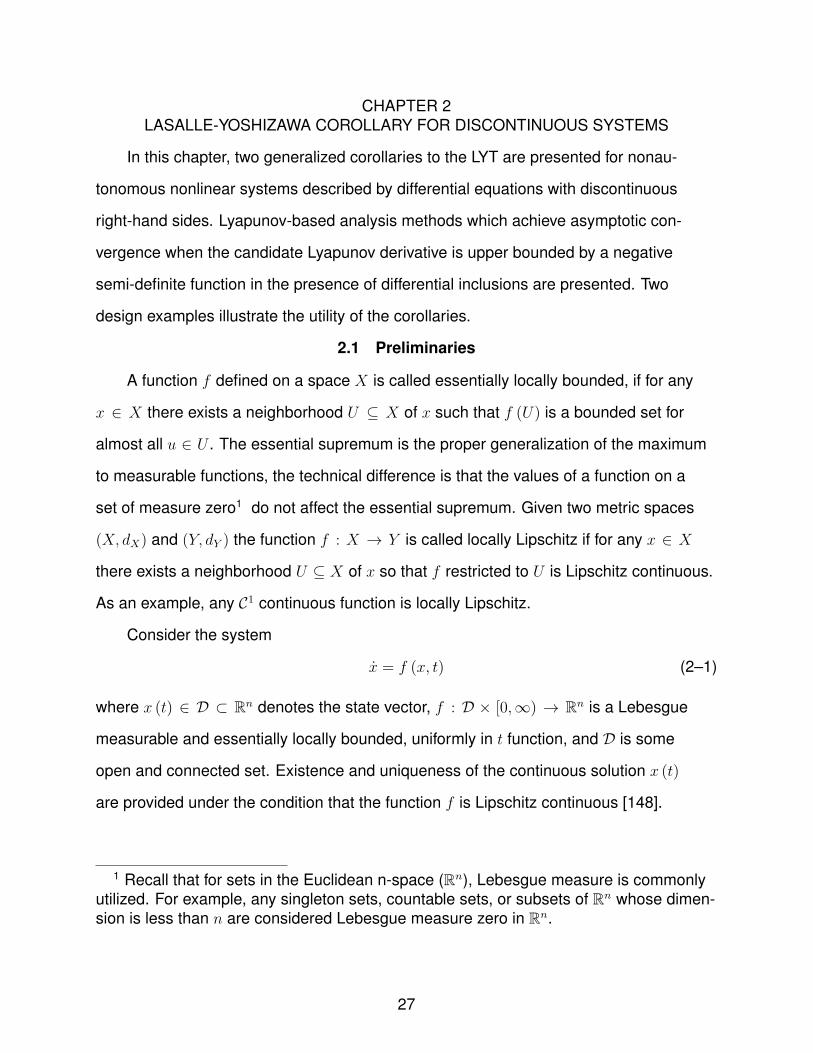
Consider the differential system given by

x = f (x, t) + g (x, t) (2–3)

where f (x, t) = sgn (x) and g (x, t) = sin (x). Based on Definition 2.1, the Filippov

solution for the system in (2–3) is given by

x ∈ K [f + g] (x, t) .

Based on the calculus for K [·] developed in [154], K [f + g] (x) ⊆ K [f ] (x, t)+K [g] (x, t).

For continuous functions, the differential inclusion evaluated at every point is equivalent

to the continuous function evaluated at that point, i.e, K [g] (x, t) = g (x, t). To examine

how the differential inclusion is computed, first note that the sets (of Lebesgue measure

zero) of discontinuity for f (x, t) include the singleton set 0.

When x > 0 or x < 0, it is straight forward to compute that the expressions for

K [f ] (·) reduce to the singletons 1 and −1, respectively. An illustration of the

positive case is depicted in Figure 2-1 where ∀δ (only 3 of the infinite sizes are shown),

the function f evaluated at the appropriate reduced set is equivalent to K [f ] (x+) =

co −1, 1∩ co −1, 1∩ co 1∩ .... Computing the closed convex hull of each intersection

reduces the inclusion to K [f ] (x+) = [−1, 1] ∩ [−1, 1] ∩ 1 ∩ ... = 1. The same

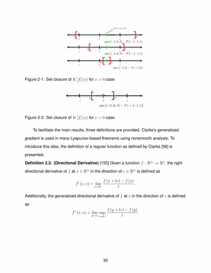
arguments can be used to compute the differential inclusion for x < 0.

At x = 0, the expression for K [f ] (x) reduces to K [f ] (0) =⋂δ>0

co [sgn (B (0, δ)− 0)].

Since B (0, δ), δ > 0, an open interval containing the origin, intersects both (0,∞) and

(−∞, 0) on sets of positive measure, K [f ] (0) =⋂δ>0

co [sgn ([x− δ, x+ δ]− 0)] =

co −1, 1 = [−1, 1]. This closure is illustrated in Figure 2-2.

Thus it is easy to see that the differential inclusion can be described by x ∈

SGN (x) + sin (x) where SGN (·) is the set-valued sign function defined by SGN (x) = 1

if x > 0, [−1, 1] if x = 0, and −1 if x < 0. So at x 6= 0, x ∈ K [f + g] is a singleton and at

x = 0, x ∈ K [f + g] is a set.

29

-1 1 0 -11-δ δ

Pick any x>0

-1 1 0 -δ δ

1

-1 1 0 -δ δ

Figure 2-1. Set closure of K [f ] (x) for x > 0 case.

-1 1 0

-δ δ

Figure 2-2. Set closure of K [f ] (x) for x = 0 case.

To facilitate the main results, three definitions are provided. Clarke’s generalized

gradient is used in many Lyapunov-based theorems using nonsmooth analysis. To

introduce this idea, the definition of a regular function as defined by Clarke [56] is

presented.

Definition 2.2. (Directional Derivative) [155] Given a function f : Rm → Rn, the right

directional derivative of f at x ∈ Rm in the direction of v ∈ Rm is defined as

f ′ (x, v) = limt→0+

f (x+ tv)− f (x)

t.

Additionally, the generalized directional derivative of f at x in the direction of v is defined

as

f o (x, v) = limy→x

supt→0+

f (y + tv)− f (y)

t.

30

Definition 2.3. (Regular Function) [56] A function f : Rm → Rn is said to be regular at

x ∈ Rm if for all v ∈ Rm, the right directional derivative of f at x in the direction of v exists

and f ′ (x, v) = f o (x, v).2

The following Lemma provides a method for computing the time derivative of a

regular function V using Clarke’s generalized gradient [56] and K [f ] (x, t) along the

solution trajectories of the system in (2–1).

Definition 2.4. (Clarke’s Generalized Gradient) [56] For a function V : Rn × R → R

that is locally Lipschitz in (x, t), define the generalized gradient of V at (x, t) by

∂V (x, t) = co lim∇V (x, t) | (xi, ti)→ (x, t) , (xi, ti) /∈ ΩV

where ΩV is the set of measure zero where the gradient of V is not defined.

Definition 2.5. (Locally bounded, uniformly in t) Let f : D × [0,∞) → R. The map

x→ f (x, t) is locally bounded, uniformly in t, if for each compact set K ⊂ D, there exists

c > 0 such that |f (x, t)| ≤ c, ∀ (x, t) ∈ K × [0,∞).

Lemma 2.1. (Chain Rule) [45] Let x (t) be a Filippov solution of system (2–1) and

V : D × [0,∞)→ R be a locally Lipschitz, regular function. Then V (x (t) , t) is absolutely

continuous, ddtV (x (t) , t) exists almost everywhere (a.e.), i.e., for almost all t ∈ [0,∞),

and V (x (t) , t)a.e.∈ ˙V (x (t) , t) where

˙V (x, t) ,⋂

ξ∈∂V (x,t)

ξT

K [f ] (x, t)

1

.Remark 2.2. Throughout the subsequent discussion, for brevity of notation, let a.e. refer

to almost all t ∈ [0,∞).

2 Note that any C1 continuous function is regular and the sum of regular functions isregular [156].

31

2.2 Main Result

For the system described in (2–1) with a continuous right-hand side, existing

Lyapunov theory can be used to examine the stability of the closed-loop system using

continuous techniques such as those described in [148]. However, these theorems

must be altered for the set-valued map ˙V (x (t) , t) for systems with right-hand sides

which are not Lipschitz continuous [10, 11, 45]. Lyapunov analysis for nonsmooth

systems is analogous to the analysis used for continuous systems. The differences

are that differential equations are replaced with inclusions, gradients are replaced with

generalized gradients, and points are replaced with sets throughout the analysis. The

following presentation and subsequent proofs demonstrate how the LYT can be adapted

for such systems.

The following auxiliary lemma from [154] and Barbalat’s Lemma are provided to

facilitate the proofs of the nonsmooth LYC.

Lemma 2.2. [154] Let x (t) be any Filippov solution to the system in (2–1) and V :

D × [0,∞) → R be a locally Lipschitz, regular function. If V (x (t) , t)a.e.

≤ 0, then

V (x (t) , t) ≤ V (x (t0) , t0) ∀t > t0.

Proof. For the sake of contradiction, let there exist some t > t0 such that V (x (t) , t) >

V (x (t) , t0). Then,

ˆ t

t0

V (x (σ) , σ) dσ = V (x (t) , t)− V (x (t) , t0) > 0.

It follows that V (x (t) , t) > 0 on a set of positive measure, which contradicts that

V (x (t) , t) ≤ 0, a.e.

The following Lemma recalls Barbalat’s lemma for nonautonomous systems, which

will be used in the proof of the nonsmooth LYC.

32

Lemma 2.3. (Barbalat’s Lemma) [148] Let φ : R → R be a uniformly continuous (UC)

function on [0,∞). Suppose that limt→∞

´ t0φ (τ) dτ exists and is finite. Then,

φ (t)→ 0 as t→∞.

Based on Lemmas 2.2 and 2.3, nonsmooth corollaries to the LYT (c.f., [55, Theo-

rem 8.4] and [68, Theorem A.8]) are provided in Corollary 2.1 and 2.2.

Corollary 2.1. For the system in (2–1), let D ⊂ Rn be an open and connected set

containing x = 0 and suppose f is Lebesgue measurable and essentially locally

bounded, uniformly in t. Let V : D× [0,∞)→ R be locally Lipschitz and regular such that

W1 (x) ≤ V (x, t) ≤ W2 (x) ∀t ≥ 0, ∀x ∈ D (2–4)

V (x (t) , t)a.e.

≤ −W (x (t)) (2–5)

where W1 and W2 are continuous positive definite functions, and W is a continuous

positive semi-definite function on D. Choose r > 0 and c > 0 such that Br ⊂ D and c <

min‖x‖=r

W1 (x) and x (t) is a Filippov solution to (2–1) where x (t0) ∈ x ∈ Br |W2 (x) ≤ c.

Then x (t) is bounded and satisfies

W (x (t))→ 0 as t→∞.

Proof. Since Br ⊂ D and c < min‖x‖=r

W1 (x), x ∈ Br |W1 (x) ≤ c is in the interior of Br.

Define a time-dependent set Ωt,c by

Ωt,c = x ∈ Br | V (x, t) ≤ c .

From (2–4), the set Ωt,c contains x ∈ Br |W2 (x) ≤ c since

W2 (x) ≤ c⇒ V (x, t) ≤ c.

33

On the other hand, Ωt,c is a subset of x ∈ Br |W1 (x) ≤ c since

V (x, t) ≤ c⇒ W1 (x) ≤ c.

Thus,

x ∈ Br |W2 (x) ≤ c ⊂ Ωt,c ⊂ x ∈ Br |W1 (x) ≤ c ⊂ Br ⊂ D.

Based on (2–5), V (x (t) , t)a.e.

≤ 0, hence, V (x (t) , t) is non-increasing from Lemma

2.2. For any t0 ≥ 0 and any x (t0) ∈ Ωt0,c, the solution starting at (x (t0) , t0) stays in

Ωt,c for every t ≥ t0. Therefore, any solution starting in x ∈ Br |W2 (x) ≤ c stays in

Ωt,c, and consequently in x ∈ Br |W1 (x) ≤ c, for all future time. Hence, the Filippov

solution x (t) is bounded such that ‖x (t)‖ < r, ∀t ≥ t0.

From Lemma 2.2, V (x (t) , t) is also bounded such that V (x (t) , t) ≤ V (x (t0) , t0).

Now, since V (x (t) , t) is Lebesgue measurable from (2–5),

ˆ t

t0

W (x (τ)) dτ ≤ −ˆ t

t0

V (x (τ) , τ) dτ = V (x (t0) , t0)−V (x (t) , t) ≤ V (x (t0) , t0) . (2–6)

Therefore,´ tt0W (x (τ)) dτ is bounded ∀t > t0. Existence of lim

t→∞

´ tt0W (x (τ)) dτ is guar-

anteed since the left-hand side of (2–6) is monotonically nondecreasing (based on the

definition of W (x) in (2.1)) and bounded above. Since x (t) is locally absolutely contin-

uous and f is essentially locally bounded, uniformly in t, x (t) is uniformly continuous.3

Because W (x) is continuous in x and x is on the compact set Br, W (x (t)) is uniformly

continuous in t on (t0,∞]. Therefore, by Lemma 2.3, it concludes that

W (x (t))→ 0 as t→∞. (2–7)

3 Since x (t) is locally absolutely continuous, |x(t2)− x(t1)| =∣∣∣´ t2t1 x(t)dt

∣∣∣. From the as-sumption that x → f (x, t) is essentially locally bounded, uniformly in t and since x ∈L∞, then, x ∈ L∞. Using the fact that defining x (t) on a set of zero measure does notchange x implies that

∣∣∣´ t2t1 x(t)dt∣∣∣ ≤ ∣∣∣´ t2t1 Mdt

∣∣∣, where M is a constant. Thus,∣∣∣´ t2t1 Mdt

∣∣∣ =

M |t2 − t1|, hence x (t) is uniformly continuous.

34

Remark 2.3. From Def. 2.1, K [f ] (x, t) is an upper semi-continuous, nonempty, compact

and convex valued map. While existence of a Filippov solution for any arbitrary initial

condition x (t0) ∈ D is provided by the definition, generally speaking, the solution is

non-unique [149,151].

Note that Corollary 2.1 establishes (2–7) for a specific x (t). Under the stronger

condition that4 ˙V (x, t) ≤ W (x) ∀x ∈ D, it is possible to show that (2–7) holds for all

Filippov solutions of (2–1). The next corollary is presented to illustrate this point.

Corollary 2.2. For the system given in (2–1), let D ⊂ Rn be a domain containing x = 0

and suppose f is Lebesgue measurable and essentially locally bounded, uniformly in t.

Let V : D × [0,∞)→ Rbe locally Lipschitz and regular such that

W1 (x) ≤ V (x, t) ≤ W2 (x) (2–8)

˙V (x, t) ≤ −W (x) (2–9)

∀t ≥ 0, ∀x ∈ D where W1 and W2 are continuous positive definite functions, and

W is a continuous positive semi-definite function on D. Choose r > 0 and c > 0

such that Br ⊂ D and c < min‖x‖=r

W1 (x). Then, all Filippov solutions of (2–1) such that

x (t0) ∈ x ∈ Br |W2 (x) ≤ c are bounded and satisfy

W (x (t))→ 0 as t→∞. (2–10)

Proof. Let x (t) be any arbitrary Filippov solution of (2–1). Then, from Lemma 2.1,

and (2–9), V (x (t) , t)a.e.

≤ −W (x (t)), which is precisely the condition (2–5). Since the

4 The inequality ˙V (x, t) ≤ W (x) is used to indicate that every element of the set˙V (x, t) is less than or equal to the scalar W (x).

35

selection of x (t) is arbitrary, Corollary 2.1 can be used to imply that the result in (2–7)

holds for each x (t).

2.3 Design Example 1 (Adaptive + Sliding Mode)

The LYC (and the LaSalle-Yoshizawa Theorem) are useful in its ability to provide

boundedness and convergence of solutions, while providing a compact framework

to define the region of attraction for which boundedness and convergence results

hold. In fact, the region of attraction is provided as part of the corollary structures.

In the case of semi-global and local results, these domains and sets are especially

useful. It is important to note that Barbalat’s Lemma can be used to achieve the same

results (in fact, it is used in the proof for Corollary 2.1); however, the use of Barbalat’s

Lemma would require the identification of the region of attraction for which convergence

holds and does not provide boundedness of the trajectories. For illustrative purposes,

the following design example targets the regulation of a first order nonlinear system.

Corollary 2.1 and 2.2 can also be directly applied to general nth order time-varying

nonlinear systems and to tracking control problems.

To illustrate the utility of Corollary 2.2, consider a first order nonlinear differential

equation given by

x = f (x, t) + d (x, t) + u (t) (2–11)

where f : Rn × [0,∞) → Rn is an unknown, linear-parameterizable, essentially locally

bounded, uniformly in t function that can be expressed as f (x, t) = Y (x, t) θ when

θ ∈ Rp is a vector of unknown constant parameters, and Y : Rn × [0,∞)→ Rn×p × [0,∞)

is the regression matrix for f (x, t), u : [0,∞) → Rn is the control input, x (t) ∈ Rn is

the measurable system state, and d (x, t) is an essentially locally bounded disturbance

which satisfies

‖d (x, t)‖ ≤ c1 + c2 (‖x‖) ‖x‖ (2–12)

36

where c1 ∈ R+ is a positive constant, and c2 (‖x‖) : R+ → R+ is a positive, globally

invertible, state-dependent function. A regulation controller for (2–11) can be designed

as

u (x, t) , −k1x− k2sgn (x)− Y θ (2–13)

where θ (x, t) ∈ Rp is the estimate of θ, k1, k2 ∈ R+ are gain constants, and sgn (·) is

defined ∀ξ ∈ Rn =

[ξ1 ξ2 ... ξn

]Tas sgn (ξ) ,

[sgn (ξ1) sgn (ξ2) ... sgn (ξn)

]T.

Based on the subsequent stability analysis, an adaptive update law can be defined as

˙θ = ΓY Tx (2–14)

where Γ ∈ Rn×n is a positive gain matrix. The closed-loop system is given by

x = Y θ + d (x, t)− k1x− k2sgn (x) (2–15)

where θ ∈ Rp denotes the mismatch θ , θ − θ. In (2–15), it is apparent that the

RHS contains a discontinuity in x (t) and requires the use of differential inclusions to

provide existence of solutions. Let y(x, θ)∈ Rn+p denote y ,

x

θ

and choose a

positive-definite, locally Lipschitz, regular Lyapunov candidate function as

V (y) =1

2xTx+

1

2θTΓ−1θ. (2–16)

The candidate Lyapunov function in (2–16) satisfies the following inequalities:

W1 (y) ≤ V (y) ≤ W2 (y) (2–17)

where the continuous positive-definite functions W1 (y) ,W2 (y) ∈ R are defined as

W1 (y) , λ1 ‖y‖2, W2 (y) , λ2 ‖y‖2 and λ1, λ2 ∈ R+ are known constants. Then,

37

V (y (t) , t)a.e.∈ ˙V (y (t) , t) and

˙V =⋂

ξ∈∂V (x,θ,t)

ξTK

x

˙θ

1

(x, θ, t

).

Since V (y, t) is C∞ in y,5

˙V ⊂ ∇V TK

x

˙θ

(x, θ) ⊂ [xT , θTΓ−1]K

x

˙θ

(x, θ) . (2–18)

After using (2–15), the expression in (2–18) can be written as

˙V ⊂ xT(Y θ + d (x, t)− k1x− k2K [sgn (x)]

)− θTΓ−1 ˙

θ (2–19)

where K [sgn(x)] = SGN (x) such that SGN (xi) = 1 if xi > 0, [−1, 1] if xi = 0, and −1 if

xi < 0 ∀i = 1, 2, ..., n.

Remark 2.4. One could also consider the discontinuous function instead of the differ-

ential inclusion (i.e., the sgn (·) function can alternatively be defined as sgn (0) = 0)

using Caratheodory solutions; however, this method lacks would not be an indicator

for what happens when measurement noise is present in the system. As described in

results such as [157–159], Filippov and Krasovskii solutions for discontinuous differential

equations are appropriate for capturing the possible closed-loop system behavior in

the presence of arbitrarily small measurement noise. By utilizing the set valued map

SGN (·) in the analysis, we account for the possibility that when the true state satisfies

5 For continuously differentiable Lyapunov candidate functions, the generalized gradi-ent reduces to the standard gradient. However, this is not required by the Corollary itselfand only assists in evaluation.

38

x = 0, sgn (x) (of the measured state) falls within the set [−1, 1]. Therefore, the pre-

sented analysis is more robust to measurement noise than an analysis that depends on

sgn (0) to be defined as a known singleton.

Substituting for the adaptive update law in (2–14), canceling terms and utilizing the

bound for d (x, t) in (2–12), the expression in (2–18) can be upper bounded as

˙V ≤ −k1 ‖x‖2 + c1 ‖x‖+ c2 (‖x‖) ‖x‖2 − k2 ‖x‖ . (2–20)

The set in (2–19) reduces to the scalar inequality in (2–20) since in the case when

K [sgn (x)] is defined as a set, it is multiplied by x, i.e., when x = 0, 0 · SGN (0) = 0.

Regrouping similar terms, the expression in (2–20) can be written as

˙V ≤ − (k1 − c2 (‖x‖)) ‖x‖2 − (k2 − c1) ‖x‖ . (2–21)

Provided k2 > c1 and k1 > c2 (‖x‖), the expression in (2–21) can be upper bounded

as ˙V ≤ −W (y (t)) where W (y) is a positive semi-definite function defined on the

domain D ,y | ‖y‖ < c−1

2 (k1)

. The inequalities in (2–17) can be used to show that

V (y (t) , t) ∈ L∞ in D; hence, x (t) and θ (x (t) , t) ∈ L∞ in D. Since θ contains the

constant unknown system parameters and θ (x (t) , t) ∈ L∞ in D, the definition for

θ (x (t) , t) can be used to show that θ (x (t) , t) ∈ L∞ in D. Given that x (t) ∈ L∞ in D,

Y (x (t) , t) ∈ L∞ in D. Since x (t) , θ (x (t) , t) , and Y (x (t) , t) ∈ L∞ in D, the control

is bounded from (2–13) and the adaption law in (2–14). The closed-loop dynamics in

(2–12) and (2–15) can be used to conclude that x (t) ∈ L∞ in D; hence, x (t) is uniformly

continuous in D.

Choose 0 < r < c−12 (k1) such that Br ⊂ D denotes a closed ball, and let S ⊂ Br

denote the set defined as

S ,

y ⊂ Br |W2 (y) < min

‖y‖=rW1 (y) = λ1r

2

. (2–22)

39

Invoking Corollary 2.2, W (y (t)) = − (k1 − c2 (‖x‖)) ‖x‖2 → 0 as t→∞ ∀y (0) ∈ S, thus,

x→ 0 as t→∞ ∀y (0) ∈ S. The region of attraction in (2–22) can be made arbitrarily

large to include all initial conditions (a semi-global type result) by increasing the gain k1.

Remark 2.5. For some systems (e.g., closed-loop error systems with sliding mode

control laws), it may be possible to show that Corollary 2.2 is more easily applied, as

is the focus of the first example. However, in other cases, it may be difficult to satisfy

the inequality in (2–9). The usefulness of Corollary 2.1 is demonstrated in those cases

where it is difficult or impossible to show that the inequality in (2–9) can be satisfied, but

it is possible to show that (2–5) can be satisfied for almost all time, as is the focus of the

next example.

2.4 Design Example 2 (RISE)

To illustrate the utility of Corollary 2.1, consider a second order nonlinear differential

equation given by

x = f (x, t) + d (t) + u (t) (2–23)

where f : Rn × [0,∞) → Rn is an unknown essentially locally bounded, uniformly

in t function, u : [0,∞) → Rn is the control input, x (t) ∈ Rn is the measurable

system state, and d (t) ∈ Rn is an essentially locally bounded disturbance, which

satisfies d (t) , d (t) , d (t) ∈ L∞. A desired trajectory, denoted by xd ∈ Rn, satisfies

x(i)d (t) ∈ Rn, ∀i = 0, 1, ..., 4.

To quantify the control objective, a tracking error, denoted by e1 (η, ηd) ∈ R6, is

defined as

e1 , xd − x, (2–24)

and two auxiliary tracking errors denoted by e2 (e1, e1) , r (e2, e2) ∈ R6, are defined as

e2 , e1 + α1e1, (2–25)

r , e2 + α2e2 (2–26)

40

where α1, α2 ∈ R+ are adjustable gains. The auxiliary signal r (e2, e2) is introduced to

facilitate the stability analysis and is not used in the control design since the expression

in (2–25) depends on the unmeasurable state x (t).

The open loop error system can be expressed as

r = xd + S − f (xd, t)− d (t)− u (t) + α2e2 (2–27)

where the auxiliary function S ∈ Rn is defined as S , f (xd, t) − f (x, t) + α1e1 + α2e2. A

RISE-based control structure [8,160] can be designed as

u , (ks + 1) e2 − (ks + 1) e2 (0) + υ. (2–28)

where υ (e2) ∈ Rn is the Filippov solution to the following differential equation

υ , (ks + 1)αe2 + βsgn (e2) , υ (0) = 0, (2–29)

β, ks ∈ R are positive, constant control gains and sgn (·) is defined ∀ξ ∈ Rm =[ξ1 ξ2 ... ξm

]Tas sgn (ξ) ,

[sgn (ξ1) sgn (ξ2) ... sgn (ξm)

]T. The differential

equation given in (2–29) is continuous except when e2 = 0. Using Filippov’s theory

of differential inclusions [149, 161–163], the existence of solutions can be established

for υ ∈ K [h1] (e2), where h1 (e2) ∈ Rn is defined as the right-hand side of (2–29) and

K [h1] ,⋂δ>0

⋂µSm=0

coh1 (B (e2, δ)− Sm), where⋂

µSm=0

denotes the intersection of all

sets Sm (of Lebesgue measure zero) of discontinuities, co denotes convex closure, and

B (e2, δ) = ς ∈ R| ‖e2 − ς‖ < δ [45,154].

To facilitate the subsequent analysis, the controller in (2–28) is substituted into

(2–27) and the time derivative found by utilizing a DCAL approach to regroup terms as

r = N +Nd − e2 − (ks + 1) r − βsgn (e2) (2–30)

where N (e2, r, t) ∈ Rn and Nd (t) ∈ Rn are defined as

N , S + e2, (2–31)

41

Nd ,...x d − f (xd, xd, t) + d (t) . (2–32)

Using (2–24)-(2–25) and the Mean Value Theorem, the function N (·) in (2–31) can be

upper bounded as [164, App A] ∥∥∥N∥∥∥ ≤ ρ (‖z‖) ‖z‖ , (2–33)

where z (e1, e2, r) ∈ R3n is defined as

z ,

[eT1 eT2 rT

]T(2–34)

and ρ : R → R is a positive, globally invertible, nondecreasing function. Assuming the

disturbance and desired trajectory are sufficiently smooth, the following inequalities can

be developed:

‖Nd‖ ≤ ζ1,∥∥∥Nd

∥∥∥ ≤ ζ2

where ζ1, ζ2 ∈ R+ are known constants.

Let y (z, P ) ∈ R3n+1 be defined as

y ,

[zT√P

]T(2–35)

where the auxiliary function P (e2, t) ∈ R is defined as the Filippov solution to the

following differential equation

P=−rT (Nd − βsgn (e2))

P (e2 (t0) , t0)=βn∑i=1

|e2i (t0)| − e2 (t0)T Nd (t0) (2–36)

where the subscript i = 1, 2, ..., n denotes the ith element of the vector. Similar to the

development in (2–29), existence of solutions for P can be established using Filippov’s

theory of differential inclusions for P ∈ K [h2] (e2, r, t), where h2 (e2, r, t) ∈ R is defined as

h2 , −rT (Nd − βsgn (e2)) and K [h2] ,⋂δ>0

⋂µSm=0

coh2 (B (e2, δ)− Sm, r, t) as in (2–29).

Integrating (2–36) by parts and provided β > ζ1 + ζ2α2

, P (e2, t) ≥ 0 (see [165] for details).

42

Let VL : D × [0,∞) → R be continuously differentiable in y, locally Lipschitz in t,

regular, and defined as

VL =1

2eT1 e1 +

1

2eT2 e2 +

1

2rT r + P (2–37)

which satisfies the following inequalities:

U1 (y) ≤ VL (y, t) ≤ U2 (y) , (2–38)

where U1 (y), U2 (y)∈ R are positive definite functions defined as U1 , λ1 ‖y‖2 and

U2 , λ2 ‖y‖2.

Under Filippov’s framework, the time derivative of (2–37) exists almost everywhere

(a.e.), i.e., for almost all t ∈ [0,∞), and VL (y, t)a.e.∈ ˙VL (y, t) where

˙VL =⋂

ξ∈∂VL(y,t)

ξTK

[eT1 eT2 rT 1

2P−

12 P 1

]T,

where ∂VL is the generalized gradient of VL (y, t) [45,154,166]. Since V (y, t) is C∞ in y,

˙VL ⊂ ∇V TL K

[eT1 eT2 rT 1

2P−

12 P

]T, (2–39)

where ∇VL ,

[eT1 eT2 rT 2P

12

]T.

Using the calculus for K [·] from [154], substituting (2–24), (2–25), (2–28), (2–30),

and (2–36), and canceling similar terms, the expression in (2–39) becomes

˙VL⊂eT1 e2 − α1eT1 e1 − α2e

T2 e2 + rT N + rTNd − (ks + 1) rT r

−rTβK [sgn (e2)]− rT (Nd − βK [sgn (e2)]) , (2–40)

43

where K [sgn(e2)] = SGN (e2) such that SGN (e2i) = 1 if e2i (·) > 0, [−1, 1] if e2i (·) = 0,

and −1 if e2i (·) < 0.6 Utilizing the fact that the set in (2–40) reduces to a scalar equality

since the RHS is continuous a.e., i.e, the RHS is continuous except for the Lebesgue

negligible set of times when rTβK [sgn (e2)] − rTβK [sgn (e2)] 6= 0 [45, 167], an upper

bound for VL is given as

VLa.e.

≤ −α1 ‖e1‖2 + ‖e1‖ ‖e2‖ − α2 ‖e2‖2

+ρ (‖z‖) ‖r‖ ‖z‖ − (ks + 1) ‖r‖2 . (2–41)

To show that the number of times when rTβK [sgn (e2)] − rTβK [sgn (e2)] 6= 0 is

measure zero, we recall the error system definition in (2–26) and introduce the following

lemma.

Lemma 2.4. Let f : [0,∞) → R be a continuously differentiable function with the

property: f (x) = 0, f ′ (t) 6= 0, then

µ(f−1 (0)

)= 0, (2–42)

where µ denotes the Lebesgue measure on [0,∞).

Proof. We will first prove that all the points in the set f−1 (0) are isolated. That is,

(∀a ∈ f−1 (0)

)(∃ε > 0) |

(((a− ε, a+ ε) ∩

(f−1 (0)

))\ a = φ

). (2–43)

To obtain a contradiction, the negation of the statement above is,

(∃a ∈ f−1 (0)

)| (∀ε > 0)

(((a− ε, a+ ε) ∩

(f−1 (0)

))\ a 6= φ

). (2–44)

6 As in the previous example, the sgn (·) function can alternatively be defined assgn (0) = 0; however, this restriction lacks robustness with respect to measurementnoise.

44

Assuming (2–44), let b ∈ ((a− ε, a+ ε) ∩ (f−1 (0))) \ a. Without loss of generality we

can assume b > a and f ′ (a) > 0. As f is differentiable and f (a) = f (b) = 0, by Rolle’s

theorem, ∃c ∈ (a, b) such that

f ′ (c) = 0. (2–45)

By continuity of f ′ at a,

(∀εa > 0) (∃δa > 0) | (∀x ∈ [0,∞)) (|x− a| < δa =⇒ f ′ (a)− εa < f ′ (x) < f ′ (a) + εa) .

In particular, pick εa = f ′ (a) . Then,

(∃δa > 0) | (∀x ∈ [0,∞)) (|x− a| < δa =⇒ f ′ (x) > 0) .

Now, pick ε = δa in (2–44). Thus from b ∈ ((a− δa, a+ δa) ∩ (f−1 (0))) \ a we get

|b− a| < δa which from c ∈ (a, b) implies |c− a| < δa which implies f ′ (c) > 0, which

contradicts (2–45).

Thus, all the points in the set f−1 (0) are isolated, and hence, f−1 (0) is a

discrete set. As any discrete subset of Euclidean space is countable, (2–42) is obtained.

The set of times

Λ ,t ∈ [0,∞) : r (t)T βK [sgn (e2 (t))]− r (t)T βK [sgn (e2 (t))] 6= 0

⊂ [0,∞)

is equivalent to the set of times t : e2 (t) = 0 ∧ r (t) 6= 0. From (2–26), this set can

also be represented by t : e2 (t) = 0 ∧ e2 (t) 6= 0. Provided e2 (t) is continuously

differentiable (it is in our case), Lemma 2.4 can be used to show that the set of time

instances t : e2 (t) = 0 ∧ e2 (t) 6= 0 is isolated, and thus, measure zero. This implies

that the set Λ is measure zero.

Utilizing Young’s Inequality, the expression in (2–41) can be reduced to

VLa.e.

≤ −σ ‖z‖2 − ks ‖r‖2 + ρ (‖z‖) ‖r‖ ‖z‖ , (2–46)

45

where σ = minα1 − 1

2, α2 − 1

2, 1

and z (e1, e2, r) was defined in (2–34). If the gains

are selected such that α1 >12

and α2 >12, and by completing the squares for r (·), the

expression in (2–46) can be upper bounded as

VLa.e.

≤ −σ ‖z‖2 +ρ2 (‖z‖) ‖z‖2

4ks≤ −U (y) , (2–47)

where U (y) , c ‖z‖2, for some positive constant c ∈ R, is a continuous positive

semi-definite function such that

D ,y ∈ R3n+1 | ‖y‖ ≤ ρ−1

(2√σks

).

The size of the domain D can be enlarged by increasing the gain ks. The inequalities in

(2–38) and (2–47) can be used to show that VL ∈ L∞ in D. Thus, e1 (·) , e2 (·) , r (·) ∈ L∞

in D. The closed-loop error system can be used to conclude that the remaining signals

are bounded in D, and the definitions for U (y) and z (·) can be used to show that U (y)

is uniformly continuous in D. Let SD ⊂ D denote a set defined as

SD ,

y ∈ D | U2 (y) < λ1

(ρ−1

(2√σks

))2.

The region of attraction in SD can be made arbitrarily large to include any initial con-

ditions by increasing the control gain ks. From (2–47), Corollary 2.1 can be invoked to

show that c ‖z‖2 → 0 as t → ∞ ∀y (0) ∈ SD. Based on the definition of z (·) in (2–34),

‖e1‖ → 0 as t→∞∀y (0) ∈ SD.

Remark 2.6. In Example 2.4, we apply Corollary 2.1 when VL (y, t)a.e.

≤ −W (y). The

difference in this case from Example 2.3, stems from the fact that it is not possible to

directly show that all solutions satisfy (2–9). Instead, it is possible to showthat (2–5) can

be satisfied in the analysis, and Lemma 2.4 and the associated arguments can be used

to prove that this case is satisfied for all time.

46

2.5 Summary

This chapter introduced the mechanics required to utilize nonsmooth analysis in

Lyapunov-based control design and have extended the LYT to differential systems with a

discontinuous RHS using Filippov differential inclusions. The result presents theoretical

tools applicable to nonlinear systems with discontinuities in the plant dynamics or in the

control structure. The generalized Lyapunov-based analysis methods are developed

using differential inclusions in the sense of Filippov to achieve asymptotic convergence

when the Lyapunov derivative is upper bounded by a negative semi-definite function.

Cases when the bound on the Lyapunov derivative holds for all possible Filippov

solutions are also considered. An adaptive, sliding mode control example and a RISE

control example are provided to illustrate the utility of the main results.

47

CHAPTER 3SATURATED RISE FEEDBACK CONTROL

In this chapter, a saturated controller is developed for a class of uncertain, second-

order, nonlinear systems which includes time-varying and non-LP functions with

bounded disturbances using a continuous control law with smooth saturation functions.

Based on the RISE control methodology, the proposed controller is able to utilize the

benefits of high gain control strategies while guaranteeing saturation limits are not

surpassed. The bounds on the control are known a priori and can be adjusted by

changing the feedback gains. The saturated controller yields asymptotic tracking despite

uncertainty and added disturbances in the dynamics. Experimental results using a

two-link robot manipulator demonstrate the performance of the proposed controller.

3.1 Dynamic Model

Consider a general class of nonlinear systems of the following form:

x = f (x, x, t) + u (x, x, t) + d (t) (3–1)

where x (t) , x (t) ∈ Rn are the generalized system states, u (x, x, t) ∈ Rn is the

generalized control input, f (x, x, t) : R2n × [0,∞) → Rn is an unknown nonlinear

C2 function, and d (t) : [0,∞) → Rn denotes a generalized, sufficiently smooth, non-

vanishing nonlinear disturbance (e.g., unmodeled effects).

The subsequent development is based on the assumption that x (t) and x (t) are

measurable outputs. Additionally, the following assumptions will be exploited.

Assumption 3.1. The nonlinear disturbance term and its first two time derivatives (i.e.,

d (t) , d (t) , d (t)) exist and are bounded by known constants [122,147,168].1

1 Many practical disturbance terms are continuous including friction (see [169, 170]),wind disturbances, wave/ocean disturbances, unmodeled sufficiently smooth distur-bances, etc.).

48

Assumption 3.2. The desired trajectory xd (t) ∈ Rn is designed such that x(i)d (t) ∈

Rn, ∀i = 0, 1, ..., 4 exist and are bounded.2

Remark 3.1. To aid the subsequent control design and analysis, the vector Tanh (·) ∈

Rn and the matrix Cosh (·) ∈ Rn×n are defined as

Tanh (ξ) , [tanh (ξ1) , ..., tanh (ξn)]T (3–2)

Cosh (ξ) , diag cosh (ξ1) , ..., cosh (ξn) (3–3)

where ξ = [ξ1, ..., ξn]T ∈ Rn. Based on the definition of (3–2), the following inequalities

hold ∀ξ ∈ Rn [78]:

‖ξ‖2 ≥n∑i=1

ln (cosh (ξi)) ≥1

2tanh2 (‖ξ‖) , ‖ξ‖ > ‖Tanh (ξ)‖

‖Tanh (ξ)‖2 ≥ tanh2 (‖ξ‖) , ξTTanh (ξ) ≥ TanhT (ξ)Tanh (ξ) . (3–4)

Throughout the paper, ‖·‖ denotes the standard Euclidean norm.

3.2 Control Development

The objective is to design an amplitude-limited, continuous controller which ensures

the system state x (t) tracks a desired trajectory xd (t). To quantify the control objective,

a tracking error denoted e1 (x, xd) ∈ Rn is defined as

e1 , xd − x. (3–5)

Embedding the control in a bounded trigonometric term is an obvious way to

limit the control authority below an a priori limit; however, by injecting these terms,

difficulty arises in the closed-loop stability analysis. This challenge is exacerbated by

the presence of integral control functions that are included to compensate for added

2 Many guidance and navigation applications utilize smooth, high-order differentiabledesired trajectories. Curve fitting methods can also be used to generate sufficientlysmooth time-varying trajectories.

49

disturbances as in this result. Motivated by these stability analysis complexities and

through an iterative analysis procedure, two measurable filtered tracking errors are

designed which include extra smooth saturation terms. Specifically, the filtered tracking

errors e2 (e1, e1, ef ) , r (e2, e2) ∈ Rn, are defined as

e2 , e1 + α1Tanh (e1) + Tanh (ef ) , (3–6)

r , e2 + α2Tanh (e2) + α3e2 (3–7)

where α1, α2, α3 ∈ R denote constant positive control gains, Tanh (·) was defined in

(3–2), and ef (e1, e2) ∈ Rn is an auxiliary signal whose dynamics are given by

ef , Cosh2 (ef ) −γ1e2 + Tanh (e1)− γ2Tanh (ef ) (3–8)

and γ1, γ2 ∈ R are constant positive control gains. The auxiliary signal r (e2, e2) is

introduced to facilitate the stability analysis and is not used in the control design since

the expression in (3–7) depends on the unmeasurable generalized state x (t). The

structure of the error systems (and included auxiliary signals) is motivated by the need

to inject and cancel terms in the subsequent stability analysis, and will become apparent

in Section 3.3.

An open-loop tracking error can be obtained by utilizing the filtered tracking error in

(3–7) and substituting from (3–1), (3–5), (3–6), and (3–8) to yield

r = S − fd + xd − d− u (t)− γ1e2 (3–9)

where the auxiliary function S (e1, e2, ef , t) ∈ Rn is defined as

S , fd − f − γ2Tanh (ef ) + α1Cosh−2 (e1) [e2 − α1Tanh (e1)− Tanh (ef )] (3–10)

+α2Tanh (e2) + α3e2 + Tanh (e1) ,

and a desired trajectory dependent auxiliary term is defined as fd = f (xd, xd, t) ∈ Rn.

50

Based on the form of (3–9) and through an iterative stability analysis, the continu-

ous controller, u (v), is designed as3

u , γ1Tanh (v) (3–11)

where v (e1, e2) ∈ Rn is the generalized Filippov solution to the following differential

equation

v = Cosh2 (v) [α2Tanh (e2)+α3e2 +βsgn (e2)−α1Cosh−2 (e1) e2 +γ2e2], v (0) = 0 (3–12)

where β ∈ R is a positive constant control gain and sgn (·) is defined

∀ξ ∈ Rm =

[ξ1 ξ2 ... ξm

]Tas sgn (ξ) ,

[sgn (ξ1) sgn (ξ2) ... sgn (ξm)

]T.4

Using Filippov’s theory of differential inclusions [149, 161–163], the existence of solu-

tions can be established for v ∈ K [h1] (e1, e2), where h1 (e1, e2) ∈ Rn is defined as the

RHS of (3–12) and K [h1] ,⋂δ>0

⋂µSm=0

coh1 (e1, B (e2, δ)− Sm), where⋂

µSm=0

denotes the

intersection of all sets Sm of Lebesgue measure zero, co denotes convex closure, and

B (e2, δ) = ς ∈ Rn| ‖e2 − ς‖ < δ [45,154].

In review of (3–5)-(3–10), the control strategy in (3–11) and (3–12) entails several

components including the development of the filtered error systems in (3–6) and (3–

7), which are composed of saturated hyperbolic tangent functions designed from the

Lyapunov analysis to cancel cross terms. The motivation for the design of (3–8) stems

from the need to inject a −γ1e2 signal into the closed-loop error system and to cancel

cross terms in the analysis. Based on the stability analysis methods associated with

3 An important feature of the controller in (3–11) is its applicability to the case whereconstraints exist on the available control. Note that the control law is upper bounded bythe adjustable control gain γ1 as ‖u‖ ≤

√n · γ1 where n is the dimension of u.

4 The initial condition for v (0, 0) is selected such that u (0) = 0.

51

the RISE control strategy [8, 147, 169, 171], an extra derivative is applied to the closed-

loop error system. The time derivative of (3–11) will include a Cosh−2(v) term. The

design of (3–12) is motivated by the desire to cancel the Cosh−2(v) term, enabling the

remaining terms to provide the desired feedback and cancel nonconstructive terms and

disturbances as dictated by the subsequent stability analysis.

The closed-loop tracking error system can be developed by taking the time deriva-

tive of (3–9), and using the time derivative of (3–11) to yield

r = N +Nd − γ1r − γ1βsgn (e2)− Tanh (e2)− e2 (3–13)

where N (e1, e2, r, ef ) ∈ Rn and Nd (xd, xd, xd, t) ∈ Rn are defined as

N , S + γ1α1Cosh−2 (e1) e2 − γ1γ2e2 + Tanh (e2) + e2, (3–14)

Nd ,...x d − fd − d. (3–15)

The structure of (3–13) is motivated by the desire to segregate terms that can be upper

bounded by state-dependent terms and terms that can be upper bounded by constants.

By applying the Mean Value Theorem (MVT), an upper bound can be developed for the

expression in (3–14) as [164, App A]∥∥∥N∥∥∥ ≤ ρ (‖w‖) ‖w‖ (3–16)

where the bounding function ρ (·) ∈ R is a positive, globally invertible, nondecreasing

function, and

w (e1, e2, r, ef ) ∈ R5n is defined as

w ,[TanhT (e1) , eT2 , r

T , TanhT (ef )]T. (3–17)

From Assumptions 3.1 and 3.2, the following inequality can be developed based on the

expression in (3–15):

‖Nd‖ ≤ ζNd1,∥∥∥Nd

∥∥∥ ≤ ζNd2(3–18)

52

where ζNd1, ζNd2

∈ R, are known positive constants.

3.3 Stability Analysis

Theorem 3.1. Given the dynamics in (3–1), the controller given by (3–11) and (3–12)

ensures asymptotic tracking in the sense that

‖e1‖ → 0 as t→∞

provided the control gains are selected sufficiently large based on the initial condi-

tions of the states (see the subsequent stability analysis) and the following sufficient

conditions

α1 >1

2, α2 > 0, α3 >

1

2+γ2

1ζ2

4, γ2 >

1

ζ2, βγ1 > ζNd1

+ζNd2

α3

. (3–19)

where α1, α2, α3, γ1, γ2 and β were introduced in (3–6)-(3–8) and (3–12), respectively,

and ζ ∈ R is a subsequently defined adjustable positive constant.

Proof. Let z (e1, e2, r, ef ) ∈ R4n be defined as

z ,[eT1 , e

T2 , r

T , TanhT (ef )]T (3–20)

and y (z, P ) ∈ R4n+1 be defined as

y ,

[zT√P

]T. (3–21)

In (3–21), the auxiliary function P (e2, t) ∈ R is defined as the generalized Filippov

solution to the following differential equation

P = −rT (Nd − βγ1sgn (e2)) , P (e2 (t0) , t0) = βγ1

n∑i=1

|e2i (t0)| − e2 (t0)T Nd (t0) (3–22)

where the subscript i = 1, 2, ..., n denotes the ith element of the vector. Similar to the

development in (3–12), existence of solutions for P (e2, t) can be established using

Filippov’s theory of differential inclusions for P ∈ K [h2] (e2, r, t), where h2 (e2, r, t) ∈ R is

defined as h2 , −rT (Nd − βγ1sgn (e2)) and K [h2] ,⋂δ>0

⋂µSm=0

coh2 (B (e2, δ)− Sm, r, t) as

53

in (3–41). Provided the sufficient condition for β in (3–19) is satisfied, P (e2, t) ≥ 0 (See

the Appendix A for details).

Let VL (y, t) : D × [0,∞)→ R be a positive-definite regular function defined as

VL ,n∑i=1

ln (cosh (e1i)) +n∑i=1

ln (cosh (e2i)) +1

2eT2 e2 +

1

2rT r

+1

2TanhT (ef )Tanh (ef ) + P (3–23)

where e1i (·) and e2i (·) denote the ith element of the vector e1 (x, xd) and e2 (e1, e1, ef ),

respectively. The Lyapunov function candidate in (3–23) satisfies the following inequali-

ties:

φ1 (y) ≤ VL (y, t) ≤ φ2 (y) . (3–24)

Based on (3–4) and (3–23), the continuous positive definite functions φ1 (y) , φ2 (y) ∈ R

in (3–24) are defined as φ1 (y) , 12tanh2 (‖y‖), φ2 (y) , 3

2‖y‖2.

Under Filippov’s framework, the time derivative of (3–23) exists almost everywhere,

i.e., for almost all t ∈ [t0, tf ], and V (y, t)a.e.∈ ˙V (y, t) where

˙VL =⋂

ξ∈∂VL(y,t)

ξTK

[eT1 eT2 rT Cosh−2 (ef ) e

Tf

1

2P−

12 P 1

]T,

∂VL is the generalized gradient of VL (y, t) [166]. Since VL (y, t) is a Lipschitz continuous

regular function,

˙VL ⊂ ∇V TL K

[eT1 eT2 rT Cosh−2 (ef ) e

Tf

1

2P−

12 P

]T(3–25)

where ∇VL ,[TanhT (e1) ,

(TanhT (e2) + eT2

), rT , TanhT (ef ) , 2P

12

]T.

54

Using the calculus for K [·] from [154], and substituting (3–5)-(3–8), and (3–13) into

(3–25), yields

˙VL ⊂ rT(N +Nd − γ1r − Tanh (e2)− e2 − γ1βK [sgn (e2)]

)+TanhT (e1) (e2 − α1Tanh (e1)− Tanh (ef )) + TanhT (e2) (r − α2Tanh (e2)− α3e2)

+eT2 (r − α2Tanh (e2)− α3e2) + TanhT (ef ) (−γ1e2 + Tanh (e1))

+TanhT (ef ) (−γ2Tanh (ef )) + P (3–26)

where K [sgn(e2)] = SGN (e2) [154] such that SGN (e2i) = 1 if e2i (·) > 0, [−1, 1] if

e2i (·) = 0, and −1 if e2i (·) < 0. Substituting (3–22), canceling common terms and

rearranging the resulting expression yields

VLa.e.= −α1Tanh

T (e1)Tanh (e1)− α2TanhT (e2)Tanh (e2)− α3e

T2 e2

−γ2TanhT (ef )Tanh (ef )− γ1r

T r + rT N + TanhT (e1) e2 − TanhT (e2)α3e2

−γ1TanhT (ef ) e2 − α2e

T2 Tanh (e2) (3–27)

where the set in (3–26) reduces to the scalar equality in (3–27) since the RHS is

continuous a.e., i.e, the RHS is continuous except for the Lebesgue measure zero set of

times when rTγ1βK [sgn (e2)] − rTγ1βK [sgn (e2)] 6= 0.5 Utilizing the definition of (3–7),

(3–16), and (3–18), the expression in (3–27) can be upper bounded as

VLa.e.

≤ −α1 ‖Tanh (e1)‖2 − (2α2 + α3) ‖Tanh (e2)‖2 − α3 ‖e2‖2 − γ2 ‖Tanh (ef )‖2 − γ1 ‖r‖2

+ρ ‖w‖ ‖r‖+ ‖Tanh (e1)‖ ‖e2‖+ γ1 ‖Tanh (ef )‖ ‖e2‖ . (3–28)

5 The set of times Λ ,t ∈ [0,∞) : r (t)T γ1βK [sgn (e2 (t))]− r (t)T γ1βK [sgn (e2 (t))] 6= 0

⊂

[0,∞) is equivalent to the set of times t : e2 (t) = 0 ∧ r (t) 6= 0. From (3–7), this set canalso be represented by t : e2 (t) = 0 ∧ e2 (t) 6= 0. Provided e2 (t) is continuously dif-ferentiable, it can be shown that the set of time instances t : e2 (t) = 0 ∧ e2 (t) 6= 0 isisolated, and thus, measure zero. This implies that the set Λ is measure zero.

55

Young Inequality can be applied to select terms in (3–28) as

‖Tanh (e1)‖ ‖e2‖ ≤1

2‖Tanh (e1)‖2 +

1

2‖e2‖2 (3–29)

γ1 ‖Tanh (ef )‖ ‖e2‖ ≤1

ζ2‖Tanh (ef )‖2 +

γ21ζ

2

4‖e2‖2 .

To facilitate the subsequent stability analysis, let γ1 be selected as γ1 = γa + γb where

γa, γb ∈ R are positive gain constants. Utilizing (3–29), completing the squares on r (·)

and grouping terms, the expression in (3–28) can be upper bounded by

VLa.e.

≤ −(α1 −

1

2

)‖Tanh (e1)‖2 − (2α2 + α3) ‖Tanh (e2)‖2 −

(α3 −

1

2− γ2

1ζ2

4

)‖e2‖2

−(γ2 −

1

ζ2

)‖Tanh (ef )‖2 − γa ‖r‖2 +

ρ2 (‖w‖) ‖w‖2

4γb. (3–30)

Provided the sufficient conditions in (3–19) are satisfied, (3–17) and (3–20) can be used

to conclude that

VLa.e.

≤ −φ3 (‖z‖) ≤ −U (y) (3–31)

where φ3 (‖z‖) ∈ R is defined as φ3 ,(λ− ρ2(‖w‖)

4γb

)tanh2 (‖z‖), λ ∈ R+ is defined as

λ = minα1 − 1

2, 2α2 + α3, α3 − 1

2− γ2

1ζ2

4, γ2 − 1

ζ2 , γa

, and U (y) , c tanh2 (‖z‖) ∀y ⊂ D

is a continuous, positive semi-definite function for some positive constant c ∈ R, where

D ,y ∈ R4n+1 | ‖y‖ ≤ ρ−1

(2√λγb

). (3–32)

The inequalities in (3–24) and (3–31) can be used to show that VL (y, t) ∈ L∞ in D,

hence,

e1 (·) , e2 (·) , r (·) , Tanh (ef (·)) ∈ L∞ in D. From (3–2), Tanh (e1) , Tanh (e2) ∈ L∞

in D. Thus, from (3–6) and (3–7), e1 (·) , e2 (·) ∈ L∞ in D. From (3–11) and (3–4),

u (·) ∈ L∞ in D. From Assumption 3.2 and by utilizing the fact that e1 (·) , e1 (·)∈ L∞,

q (t) , q (t) ∈ L∞ in D. From the above statements, (3–13) can be used to show that

r (·) ∈ L∞ in D. Since f is C2 and q (t) , q (t) ∈ L∞, f (q, q, t) ∈ L∞. Utilizing the derivative

of (3–7), Assumption 3.1 and the facts that e2 (·) , e2 (·) , r (·) , f (·) , u (·) ∈ L∞, the product

56

Cosh−2 (ef ) ef ∈ L∞. Thus, z (·) ∈ L∞ in D and it can be shown that z (·) is uniformly

continuous (UC) in D. Since z (·) is UC, tanh (‖z‖) is UC. The definitions of U (y) and

z (·) can be used to prove that U (y) is UC in D. Let S ⊂ D denote a set defined as

S ,

y ∈ D | φ2 (y) <

(ρ−1

(2√λγb

))2. (3–33)

The region of attraction in (3–33) can be made larger by increasing the control gain γb.

For arbitrarily large initial conditions or arbitrarily large disturbances, the control gains

required to satisfy the sufficient gain conditions in (3–19) may demand an input that is

not physically deliverable by the system (i.e., the gain γ1 may be required to be larger

than the saturation limit of the actuator). Despite gain dependency on the system’s initial

conditions, this result does not satisfy the standard semi-global result because under the

consideration of input constraints, γb cannot be arbitrarily increased and consequently

the region of attraction cannot be arbitrarily enlarged to include all initial conditions.6

From (3–31), Corollary 2.1 can be invoked to show that tanh (‖z‖) → 0 as t →

∞∀y (0) ∈ S. Based on the definition of z (·) in (3–20), ‖e1‖ → 0 as t→∞∀y (0) ∈ S.

3.4 Euler-Lagrange Extension

The results presented in Chapter 3 can be extended to general systems which can

be described by EL equations of motion. Specifically, consider a nonlinear system of the

form

M (q) q + Vm (q, q) q +G (q) + F (q) + τd (t) = u (t) (3–34)

where M (q) ∈ Rn×n denotes the generalized, state-dependent inertia, Vm (q, q) ∈ Rn×n

denotes the generalized centrifugal and Coriolis forces, G (q) ∈ Rn denotes the

6 This outcome is not surprising from a physical perspective in the sense that suchdemands may yield cases where the actuation is insufficient to stabilize the system.

57

generalized gravity, F (q) ∈ Rn denotes the generalized friction, τd ∈ Rn denotes a

general nonlinear disturbance (e.g., unmodeled effects), q (t) , q (t) , q (t) ∈ Rn denote the

generalized states and u (t) ∈ Rn denotes the generalized control force.

The design of the error systems and controller follow similarly to the method pre-

sented in Section 3.2. Utilizing standard properties of the inertia and centrifugal/Coriolis

matrices, and the assumptions from Section 3.1, the control development can be

extended to achieve a similar result as in Section 3.3.

Assumption 3.3. The inertia matrix M (q) is symmetric positive-definite, and satisfies

the following inequality ∀y (t) ∈ Rn :

m ‖y‖2 ≤ yTMy ≤ m (q) ‖y‖2 (3–35)

where m ∈ R is a known positive constant, m (q) ∈ R is a known positive function, and

‖·‖ denotes the standard Euclidean norm.

The error systems e1 (·), e2 (·), r (·), ef (·) are designed as in (3–5)-(3–8), respec-

tively. An open-loop error system similar to (3–9) is developed as

Mr = S +R− u (t)−Mγ1e2 (3–36)

where the auxiliary functions S (e1, e2, ef , t) ∈ Rn and R (qd, qd, qd, t) ∈ Rn are defined as

S,Mqd + Vmq +G+ F − Sd +Mα1Cosh−2 (e1) [e2 − α1Tanh (e1)− Tanh (ef )]

−Mγ2Tanh (ef ) +Mα2Tanh (e2) +Mα3e2 +MTanh (e1) , (3–37)

R , Sd + τd (3–38)

and a desired trajectory dependent auxiliary term, Sd (qd, qd, qd, t) ∈ Rn, defined as

Sd ,Mdqd + Vmdqd +Gd + Fd, (3–39)

is added and subtracted. In (3–39), Md, Vmd, Gd, Fd denote M (qd) ∈ Rn×n, Vm (qd, qd) ∈

Rn×n, G (qd) ∈ Rn, F (qd) ∈ Rn, respectively.

58

The control is designed similarly to that of (3–11) and (3–12), however several

additional terms must be included to handle terms associated with the inertia ma-

trix. Because of this, the EL extension result requires the inertia matrix to be known.

Based on the form of (3–36) and through an iterative stability analysis, the continuous

controller, u (t), is designed as

u , γ1Tanh (v) (3–40)

where v (e1, e2) ∈ Rn is the generalized Filippov solution to the following differential

equation

v=Cosh2 (v) [Mα2Tanh (e2) +Mα3e2 + βsgn (e2)

−α1Cosh−2 (e1) e2 − Me2 + γ2Me2

], (3–41)

v (0) = 0, where β ∈ R is a positive constant control gain. Because the RHS of v

contains the sgn (·) function, Filippov theory must again be used to prove existence of

solutions. Because the details follow from the previous development, they are omitted in

this extension.

The closed-loop tracking error system can be developed by inserting the control

into (3–36), taking the time derivative, and by adding and subtracting Tanh (e2) and e2 to

yield

Mr = −1

2Mr + N +Nd −Mγ1r − γ1βsgn (e2)− Tanh (e2)− e2 (3–42)

where N (e1, e2, r, ef ) ∈ Rn and Nd

(qd, qd, qd, q

(3)d , t

)∈ Rn are defined as

N , −1

2Mr + ˙S + Tanh (e2) + e2 (3–43)

and

Nd , R. (3–44)

In (3–43), ˙S (e1, e2, ef , t) ∈ Rn is defined as ˙S , S − α1γ1MCosh−2 (e1) e2 + γ1γ2Me2

where the last two terms are from the time derivative of (3–40) and cancel with inverse

59

terms inside of S (which arise due to Tanh (ef ) terms inside S) to yield ˙S free of direct

use of the gain parameter γ1. Remaining γ1 terms in ˙S are encapsulated within Tanh (·)

functions and thus can be upper bounded by 1.

Utilizing a similar Lyapunov candidate function VL (y, t) : D × [0,∞)→ R defined as

VL ,n∑i=1

ln (cosh (e1i)) +n∑i=1

ln (cosh (e2i)) +1

2eT2 e2 +

1

2rTMr

+1

2TanhT (ef )Tanh (ef ) + P, (3–45)

and Corollary 2.1, it can be shown that

VLa.e.

≤ −φ3 (‖z‖) ≤ −U (y) (3–46)

where φ3 (‖z‖) ∈ R is defined as φ3 ,(λ− ρ2(‖x‖)

4γb

)tanh2 (‖z‖), λ is defined similar to in

(3–31), and U (y) , c · tanh2 (‖z‖) for some positive constant c, is a continuous, positive

semi-definite function defined on D (defined in (3–32)). Additionally, γ1 is designed such

that γ1 , γa+γbm

where γa, γb ∈ R are positive gain constants and x (e1, e2, r, ef ) ∈ R5n is

defined the same as w in (3–17). From (3–46), tanh (‖z‖) → 0 as t → ∞ ∀y (0) ∈ S

where S is defined as

S,y ∈ D |max

1

2m (q) ,

3

2

‖y‖2 <

1

2min 1,m

(ρ−1(

2√λγb

))2

.

Based on the definition of z (·) in (3–20), it can be shown that

‖e1 (t)‖ → 0 as t→∞∀y (0) ∈ S.

Additional details regarding the EL extension of this chapter can be found in [172].

60

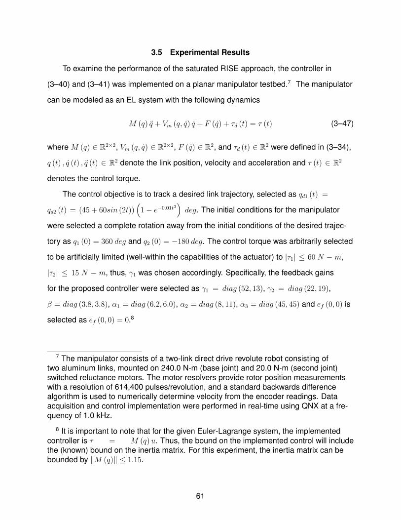
3.5 Experimental Results

To examine the performance of the saturated RISE approach, the controller in

(3–40) and (3–41) was implemented on a planar manipulator testbed.7 The manipulator

can be modeled as an EL system with the following dynamics

M (q) q + Vm (q, q) q + F (q) + τd (t) = τ (t) (3–47)

where M (q) ∈ R2×2, Vm (q, q) ∈ R2×2, F (q) ∈ R2, and τd (t) ∈ R2 were defined in (3–34),

q (t) , q (t) , q (t) ∈ R2 denote the link position, velocity and acceleration and τ (t) ∈ R2

denotes the control torque.

The control objective is to track a desired link trajectory, selected as qd1 (t) =

qd2 (t) = (45 + 60sin (2t))(

1− e−0.01t3)deg. The initial conditions for the manipulator

were selected a complete rotation away from the initial conditions of the desired trajec-

tory as q1 (0) = 360 deg and q2 (0) = −180 deg. The control torque was arbitrarily selected

to be artificially limited (well-within the capabilities of the actuator) to |τ1| ≤ 60 N − m,

|τ2| ≤ 15 N − m, thus, γ1 was chosen accordingly. Specifically, the feedback gains

for the proposed controller were selected as γ1 = diag (52, 13), γ2 = diag (22, 19),

β = diag (3.8, 3.8), α1 = diag (6.2, 6.0), α2 = diag (8, 11), α3 = diag (45, 45) and ef (0, 0) is

selected as ef (0, 0) = 0.8

7 The manipulator consists of a two-link direct drive revolute robot consisting oftwo aluminum links, mounted on 240.0 N-m (base joint) and 20.0 N-m (second joint)switched reluctance motors. The motor resolvers provide rotor position measurementswith a resolution of 614,400 pulses/revolution, and a standard backwards differencealgorithm is used to numerically determine velocity from the encoder readings. Dataacquisition and control implementation were performed in real-time using QNX at a fre-quency of 1.0 kHz.

8 It is important to note that for the given Euler-Lagrange system, the implementedcontroller is τ = M (q)u. Thus, the bound on the implemented control will includethe (known) bound on the inertia matrix. For this experiment, the inertia matrix can bebounded by ‖M (q)‖ ≤ 1.15.

61

Table 3-1. Steady-state RMS error and torque for each of the analyzed control designs.RMS Error 1 RMS Error 2 RMS Torque 1 RMS Torque 2

PID w/ AW [173] 8.3857 1.4096 14.5630 1.8732

Adaptive FSFB [174] 3.8232 1.6538 14.9367 1.2360

Saturated RISE (Proposed) 0.1607 0.2889 14.3363 1.1883

The performance of the saturated RISE control design was compared against two

controllers available in literature: a classical PID controller with conditional integral

clamping anti-windup [173] and an adaptive full-state feedback controller with bounded

inputs [174]. Each controller was tuned to achieve the best possible performance, given

the saturation bounds. Since each controller has a different structure, it is difficult to

comment on the comparative nature of the gains which were implemented. Starting

with the same large initial condition offset, the tracking errors of each controller are

depicted in Figure 3-1. The actual trajectories with respect to the desired trajectories are

shown in Figure 3-2. The control torques for each controller are shown in Figure 3-3 and

each remain within the prescribed bounds. To quantify the steady-state performance,

root mean square (RMS) errors are listed in Table 3-1. The table illustrates that for

comparable RMS torque values, the saturated RISE controller exhibits improved steady-

state performance when compared to the other control designs.

62

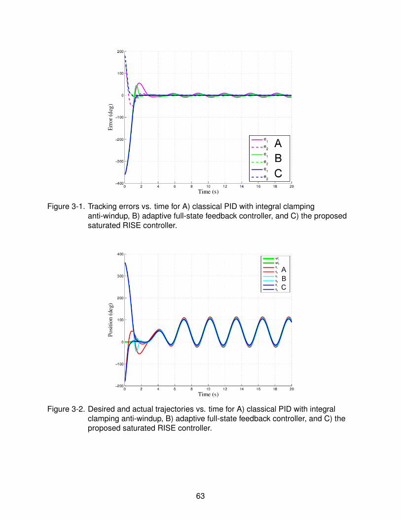
Figure 3-1. Tracking errors vs. time for A) classical PID with integral clampinganti-windup, B) adaptive full-state feedback controller, and C) the proposedsaturated RISE controller.

Figure 3-2. Desired and actual trajectories vs. time for A) classical PID with integralclamping anti-windup, B) adaptive full-state feedback controller, and C) theproposed saturated RISE controller.

63

Figure 3-3. Control torque vs. time for A) classical PID with integral clampinganti-windup, B) adaptive full-state feedback controller, and C) the proposedsaturated RISE controller.

3.6 Summary

A continuous saturated controller is developed for a class of uncertain nonlinear

systems which includes time-varying and non-LP functions and additive bounded dis-

turbances. The bound on the control is known a priori and can be adjusted by changing

the feedback gains. The saturated controller is shown to guarantee asymptotic tracking

using smooth hyperbolic functions. An extension to EL systems is presented and illus-

trated via experimental results using a two-link robot manipulator to demonstrate the

performance of the control design.

64

CHAPTER 4RISE-BASED CONTROL OF AN UNCERTAIN NONLINEAR SYSTEM WITH

TIME-VARYING STATE DELAYS

This chapter considers a continuous control design for second-order control

affine nonlinear systems with time-varying state delays. Building on previous work in

Chapters 2 and 3, a NN is augmented with a RISE control structure to achieve semi-

global asymptotic tracking in the presence of unknown, arbitrarily large, time-varying

delays, non-LP uncertainty and additive bounded disturbances. By expressing unknown

functions in terms of the desired trajectories and through strategic grouping of delay-free

and delay-dependent terms, LK functionals are utilized to cancel the delayed terms in

the analysis and obtain delay-free NN update laws.

4.1 Dynamic Model

Consider a class of uncertain second-order control affine nonlinear systems with an

unknown time-varying state delay described by

x = f (x, x, t) + g (x (t−τ) , x (t−τ) , t) + d (t) + u (t) . (4–1)

In (4–1), f (x, x, t) : R2n × [0,∞) → Rn is an unknown function, g (x (t− τ) , x (t− τ) , t) :

R2n × [0,∞) → Rn is an unknown time-delayed function, τ (t) ∈ R is an unknown, time-

varying, arbitrarily large time-delay, d (t) : [0,∞) → Rn is a sufficiently smooth bounded

disturbance (e.g., unmodeled effects), u (t) ∈ Rn is the control input, and x (t) , x (t) ∈ Rn

are measurable system states. Throughout the chapter, a time-dependent delayed

function is denoted as ζ (t− τ) or ζτ , and ‖·‖ denotes the Euclidean norm of a vector.

Following the work of Chapter 3, Assumptions 3.1 and 3.2 are utilized for the

system in (4–1). Additionally, the following assumptions are applicable:

Assumption 4.1. The unknown time delay is bounded such that 0 ≤ τ (t) ≤ ϕ1 and the

rate of change of the delay is bounded such that |τ (t)| ≤ ϕ2 < 1 where ϕ1, ϕ2 ∈ R+ are

known constants.

65

Assumption 4.2. The functions f (·) , g (·) and their first and second derivatives with

respect to their arguments are Lipschitz continuous.

4.2 Control Development

The control objective is to design a continuous controller that will ensure x (t) tracks

a desired trajectory. As in Chapter 3, a tracking error denoted e1 (x, t) ∈ Rn is defined as

e1 , xd − x. (4–2)

To facilitate the subsequent analysis, two filtered tracking errors, denoted by

e2 (e1, e1, t) , r (e2, e2, t) ∈ Rn, are defined as

e2 , e1 + α1e1 (4–3)

r , e2 + α2e2 (4–4)

where α1, α2 ∈ R+ are known gain constants. The auxiliary signal r (e2, e2, t) is intro-

duced to facilitate the stability analysis and is not used in the control design since the

expression in (4–4) depends on the unmeasurable state x (t).

An open-loop tracking error can be obtained by substituting for (4–1)-(4–4) to yield

r = α1e1 + α2e2 + xd − d

−f (x, x, t)− g (xτ , xτ , t)− u. (4–5)

Using a desired compensation adaptation law (DCAL)-based design approach [175],

(4–5) can be written as

r = α1e1 + α2e2 + S1 + Sd + xd − d

+g (xd, xd)− g (xdτ , xdτ )− u (4–6)

66

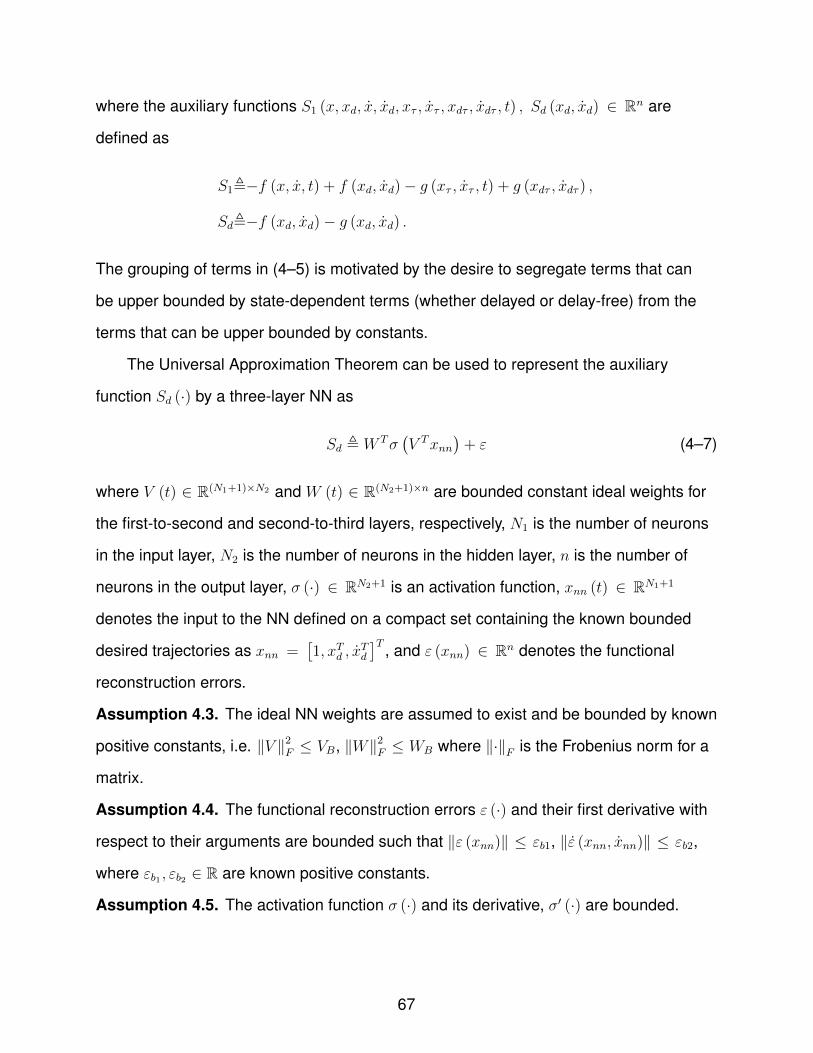
where the auxiliary functions S1 (x, xd, x, xd, xτ , xτ , xdτ , xdτ , t) , Sd (xd, xd) ∈ Rn are

defined as

S1,−f (x, x, t) + f (xd, xd)− g (xτ , xτ , t) + g (xdτ , xdτ ) ,

Sd,−f (xd, xd)− g (xd, xd) .

The grouping of terms in (4–5) is motivated by the desire to segregate terms that can

be upper bounded by state-dependent terms (whether delayed or delay-free) from the

terms that can be upper bounded by constants.

The Universal Approximation Theorem can be used to represent the auxiliary

function Sd (·) by a three-layer NN as

Sd , W Tσ(V Txnn

)+ ε (4–7)

where V (t) ∈ R(N1+1)×N2 and W (t) ∈ R(N2+1)×n are bounded constant ideal weights for

the first-to-second and second-to-third layers, respectively, N1 is the number of neurons

in the input layer, N2 is the number of neurons in the hidden layer, n is the number of

neurons in the output layer, σ (·) ∈ RN2+1 is an activation function, xnn (t) ∈ RN1+1

denotes the input to the NN defined on a compact set containing the known bounded

desired trajectories as xnn =[1, xTd , x

Td

]T , and ε (xnn) ∈ Rn denotes the functional

reconstruction errors.

Assumption 4.3. The ideal NN weights are assumed to exist and be bounded by known

positive constants, i.e. ‖V ‖2F ≤ VB, ‖W‖2

F ≤ WB where ‖·‖F is the Frobenius norm for a

matrix.

Assumption 4.4. The functional reconstruction errors ε (·) and their first derivative with

respect to their arguments are bounded such that ‖ε (xnn)‖ ≤ εb1, ‖ε (xnn, xnn)‖ ≤ εb2,

where εb1 , εb2 ∈ R are known positive constants.

Assumption 4.5. The activation function σ (·) and its derivative, σ′ (·) are bounded.

67

Remark 4.1. Assumptions 4.3-4.4 are standard assumptions in NN control literature

(cf. [176]). The ideal weight upper bounds are assumed to be known to facilitate the use

of the projection algorithm to ensure the weight estimates are always bounded. There

are numerous activations functions which satisfy Assumption 4.5, e.g., sigmoidal or

hyperbolic tangent functions.

The controller is designed using a three-layer NN feedforward term augmented by a

RISE feedback term as

u , Sd + µ. (4–8)

The RISE feedback term µ (e2, υ) ∈ Rn is defined as [8,160]

µ , (ks + 1) e2 − (ks + 1) e2 (0) + υ (4–9)

where υ (e2) ∈ Rn is the generalized Filippov solution to the following differential

equation

υ , (ks + 1)α2e2 + βsgn (e2) , (4–10)

β, ks ∈ R are positive, constant control gains, and sgn (·) is defined ∀ξ ∈ Rn =[ξ1 ξ2 ... ξn

]Tas sgn (ξ) ,

[sgn (ξ1) sgn (ξ2) ... sgn (ξn)

]T.1

Using Filippov’s theory of differential inclusions [149, 161–163], the existence of

solutions can be established for υ ∈ K [h1] (e2), where h1 (e2) ∈ Rn is defined as the

RHS of υ in (4–10) and K [h1] ,⋂δ>0

⋂µSm=0

coh1 (B (e2, δ)− Sm), where⋂

µSm=0

denotes the

intersection over all sets Sm of Lebesgue measure zero, co denotes convex closure, and

B (e2, δ) = ς ∈ Rn| ‖e2 − ς‖ < δ [45,154].

The NN feedforward term Sd (t) ∈ Rn in (4–8) is designed as

Sd , W Tσ(V Txnn

)(4–11)

1 The initial condition for v (0) is selected such that u (0) = 0.

68

where V (t) ∈ R(N1+1)×N2 and W (t) ∈ R(N2+1)×n are estimates of the ideal weights.

Based on the subsequent stability analysis, the DCAL-based weight update laws for the

NN in (4–11) are generated online as

·

W , proj(

Γ1σ′V T xnne

T2

)(4–12)

·

V , proj

(Γ2xnn

(σ′T We2

)T), (4–13)

where Γ1 ∈ R(N2+1)×(N2+1) and Γ2 ∈ R(N1+1)×(N1+1) are positive-definite, constant

symmetric control gain matrices, and σ′ (·) ∈ RN2+1 denotes the partial derivative of

σ , σ(V Txnn

).

The closed-loop dynamics are developed by substituting (4–8)-(4–11) into (4–6),

taking the time derivative, and adding and subtracting W T σ′V T xnn + W T σ′V T xnn to yield

r=α1e1 + α2e2 + S1 +...x d − d

−g (xdτ , xdτ , xdτ ) + g (xd, xd, xd)

− (ks + 1) r − βsgn (e2) + W T σ′V T xnn

+W T σ′V T xnn +W Tσ′V T xnn −W T σ′V T xnn

−W T σ′V T xnn − ˙W T σ − W T σ′

˙V Txnn + ε (4–14)

where estimate mismatches for the ideal weights, denoted V (t) ∈ R(N1+1)×N2 and

W (t) ∈ R(N2+1)×n, are defined as V (t) = V (t)− V (t) and W (t) = W (t)− W (t). Using

the NN weight update laws from (4–12) and (4–13), the expression in (4–14) can be

rewritten as

r = N +N + e2 − (ks + 1) r − βsgn (e2) (4–15)

69

where N(W , V , e1, e2, e1, e2, t

)∈ Rn and N

(W , V , t

)∈ Rn are defined as

N,α1e1 + α2e2 + S1 − e2 − proj(

Γ1σ′V T xnne

T2

)Tσ

−W T σ′proj

(Γ2xnn

(σ′T We2

)T), (4–16)

N,ND +NB. (4–17)

In (4–17), ND (xd, xd, xd,...x d, t) ∈ Rn is defined as

ND , W Tσ′V T xnn + ε+...x d − d

−g (xdτ , xdτ , xdτ ) + g (xd, xd, xd) (4–18)

and NB

(W , V , xd, xd, xd, t

)∈ Rn is separated such that

NB , NB1 +NB2 (4–19)

where NB1

(W, V, xd, xd, xd, t

), NB2

(W, V, xd, xd, xd, t

)∈ Rn are defined as

NB1 , −W T σ′V T xnn − W T σ′V T xnn,

NB2 , W T σ′V T xnn + W T σ′V T xnn.

Separating the terms in (4–17) is motivated by the fact that the different components

have different bounds [147].

Using Assumptions 3.1 and 4.1-4.5, ND (·) from (4–18) and NB (·) from (4–19) and

their time derivatives can be upper bounded as

‖ND‖ ≤ ζ1, ‖NB‖ ≤ ζ2,∥∥∥ND

∥∥∥ ≤ ζ3,∥∥∥NB

∥∥∥ ≤ ζ4 + ζ5 ‖e2‖ ,

where ζi ∈ R+, ∀i = 1, ..., 5 are known constants. Additionally, N (·) from (4–16) can be

upper bounded as

∥∥∥N∥∥∥ ≤ ρ1 (‖z‖) ‖z‖+ ρ2 (‖zτ‖) ‖zτ‖ (4–20)

70

where z (e1, e2, r) ∈ R3n denotes the vector z =

[eT1 eT2 rT

]Tand ρ1 (·) , ρ2 (·) : R→ R

are positive, globally invertible, nondecreasing functions. The upper bound for the

auxiliary function N (·) is segregated into delay-free and delay-dependent bounding

functions to eliminate the delayed terms with the use of an LK functional in the stability

analysis. Specifically, let RLK (z, t) ∈ R denote an LK functional defined as

RLK ,γ

2ks

ˆ t

t−τ(t)

ρ22 (‖z (σ)‖) ‖z (σ)‖2dσ (4–21)

where γ ∈ R+ is an adjustable constant, and ks and ρ2 (·) were introduced in (4–9) and

(4–20), respectively.

4.3 Stability Analysis

Theorem 4.1. The controller proposed in (4–8) and the weight update laws designed in

(4–12)-(4–13) ensure that the states and controller are bounded and the tracking errors

are regulated in the sense that

‖e1‖ → 0 as t→∞

provided the control gain ks introduced in (4–9) is selected sufficiently large based on

the initial conditions of the states, and the remaining control gains are selected based on

the following sufficient conditions

α1 >1

2, α2 > β2 +

1

2, β2 > ζ5,

β > ζ1 + ζ2 +1

α2

ζ3 +1

α2

ζ4, (1− ϕ2) γ > 1 (4–22)

where α1, α2, β, γ were introduced in (4–2), (4–3), (4–10) and (4–21), ϕ2 was introduced

in Assumption 4.1 and β2 is a subsequently defined gain constant.

Proof. Let D ⊂ R3n+3 be a domain containing y (e1, e2, r, P,Q,RLK) ∈ R3n+3, defined as

y ,

[z√P√Q√RLK

]. (4–23)

71

Similar to (3–22), the auxiliary function P (e2, t) ∈ R is defined as the generalized

Filippov solution to the following differential equation

P , −rT (NB1 +ND − βsgn (e2))− eT2NB2 + β2 ‖e2‖2 ,

P (e2 (t0) , t0) , β

n∑i=1

|e2i (t0)| − e2 (t0)T ND (t0) (4–24)

where the subscript i = 1, 2, ..., n denotes the ith element of the vector. Similar to

the development in (4–10), existence of solutions for P (e2, t) can be established

using Filippov’s theory of differential inclusions for P ∈ K [h2] (r, e2, e2, t), where

h2 (r, e2, e2, t) ∈ R is defined as the RHS of P . Provided the sufficient conditions in

(4–22) are satisfied, P (e2, t) ≥ 0 (See [147] for proof). Additionally, the auxiliary function

Q(W , V , t

)∈ R in (4–23) is defined as

Q ,α2

2tr(W TΓ−1

1 W)

+α2

2tr(V TΓ−1

2 V)

(4–25)

where Q ≥ 0 since Γ1 and Γ2 are constant, symmetric, and positive definite matrices and

α2 ∈ R+.

Let V (y, t) : D × [0,∞)→ R be a continuously differentiable in y, locally Lipschitz in

t, regular function defined as

V ,1

2eT1 e1 +

1

2eT2 e2 +

1

2rT r + P +Q+RLK (4–26)

which satisfies the following inequalities

φ1 (y) ≤ V (t) ≤ φ2 (y) (4–27)

where the continuous positive-definite functions φ1 (y) , φ2 (y) ∈ R are defined as

φ1 (y) , λ1 ‖y‖2, φ2 (y) , λ2 ‖y‖2 and λ1, λ2 ∈ R+ are known constants. Under Filippov’s

framework, the time derivative of (4–26) exists almost everywhere, i.e., for almost all

72

t ∈ [t0, tf ], and V (y, t)a.e.∈ ˙V (y, t) where

˙V =⋂

ξ∈∂V (y,t)

ξTK [%]

where % ∈ R3n+4 is defined as % ,

[eT1 eT2 rT 1

2P−

12 P 1

2Q−

12 Q 1

2R− 1

2LKRLK 1

]T,

and ∂V is the generalized gradient of V (y, t) [166]. Since V (y, t) is C∞,

˙V ⊂ ∇V K [·]T (4–28)

where

∇V ,

[eT1 eT2 rT 2P

12 2Q

12 2R

12LK

].

Using the calculus for K [·] from [154], and substituting (4–2)-(4–4), and (4–15),

(4–24), the time derivatives of (4–21), and (4–25) into (4–28), yields

˙V ⊂ eT1 (e2 − α1e1) + eT2 (r − α2e2) + rT(N +ND +NB1 +NB2 + e2 − (ks + 1) r

)+rT (−βK [sgn (e2)]) + β2 ‖e2‖2 − rT (NB1 +ND − βK [sgn (e2)])− eT2NB2 (4–29)

+γ

2ksρ2

2 (‖z‖) ‖z‖2 − γ (1− τ)

2ksρ2

2 (‖zτ‖) ‖zτ‖2 + tr(α2W

TΓ−11

˙W)

+ tr(α2V

TΓ−12

˙V)

where K [sgn(e2)] = SGN (e2) [154] such that SGN (e2i) = 1 if e2i (·) > 0, [−1, 1] if

e2i (·) = 0, and −1 if e2i (·) < 0. Canceling terms and utilizing the bounds from (4–20) and

Assumption 4.1, (4–29) can upper bounded as

Va.e.

≤ ‖e1‖ ‖e2‖ − α1 ‖e1‖2 − α2 ‖e2‖2 + ‖r‖ ρ1 (‖z‖) ‖z‖+ ‖r‖ ρ2 (‖zτ‖) ‖zτ‖

− (ks + 1) ‖r‖2 + β2 ‖e2‖2 +γ

2ksρ2

2 (‖z‖) ‖z‖2 − γ (1− ϕ2)

2ksρ2

2 (‖zτ‖) ‖zτ‖2(4–30)

where the set in (4–29) reduces to the scalar inequality in (4–30) since the RHS is

continuous a.e., i.e, the RHS is continuous except for the Lebesgue negligible set of

times when rTβK [sgn (e2)] − rTβK [sgn (e2)] 6= 0. Young’s Inequality can be used to

show that ‖e1‖ ‖e2‖ ≤ 12‖e1‖2+ 1

2‖e2‖2 and ‖r‖ ρ2 (‖zτ‖) ‖zτ‖ ≤ ks

2‖r‖2+ 1

2ksρ2

2 (‖zτ‖) ‖zτ‖2,

73

which allows for the following upper bound for (4–30)

Va.e.

≤ 1

2‖e1‖2 +

1

2‖e2‖2 − α1 ‖e1‖2 − α2 ‖e2‖2 − ks

2‖r‖2 − ‖r‖2 + β2 ‖e2‖2

+ ‖r‖ ρ1 (‖z‖) ‖z‖+1

2ksρ2

2 (‖zτ‖) ‖zτ‖2 +γ

2ksρ2

2 (‖z‖) ‖z‖2

−γ (1− ϕ2)

2ksρ2

2 (‖zτ‖) ‖zτ‖ . (4–31)

If (1− ϕ2) γ > 1, and by completing the squares for r (e2, e2, t), (4–31) becomes

Va.e.

≤ −(α1 −

1

2

)‖e1‖2 −

(α2 − β2 −

1

2

)‖e2‖2 − ‖r‖2

+1

2ksρ2

1 (‖z‖) ‖z‖2 +γ

2ksρ2

2 (‖z‖) ‖z‖2 . (4–32)

Regrouping similar terms, the expression can be upper bounded by

Va.e.

≤ −(λ3 −

ρ2 (‖z‖)2ks

)‖z‖2 (4–33)

where ρ2 (‖z‖) , ρ21 (‖z‖) + γρ2

2 (‖z‖) and λ3 , minα1 − 1

2, α2 − β2 − 1

2, 1

. The

bounding function ρ (‖z‖) : R → R is a positive-definite, globally invertible, nondecreas-

ing function. The expression in (4–33) can be further upper bounded by a continuous,

positive semi-definite function

Va.e.

≤ −φ3 (y) = −c ‖z‖2 ∀y ∈ D (4–34)

for some positive constant c ∈ R+ and domain D =y ∈ R3n+3 | ‖y‖ < ρ−1

(√2λ3ks

).

Larger values of ks will expand the size of the domain D . The inequalities in (4–27)

and (4–34) can be used to show that V ∈ L∞ in D . Thus, e1 (·) , e2 (·) , r (·) ∈ L∞ in D .

The closed-loop error system can be used to conclude that the remaining signals are

bounded in D , and the definitions for φ1 (·) and z (·) can be used to show that φ1 (·) is

uniformly continuous in D . Let SD ⊂ D denote a set defined as

SD ,

y ∈ D | φ2 < λ1

(ρ−1

(√2λ3ks

))2. (4–35)

74

The region of attraction in (4–35) can be made arbitrarily large to include any initial

conditions by increasing the control gain ks. From (4–34), 2.1 can be invoked to show

that c ‖z‖2 → 0 as t → ∞ ∀y (0) ∈ SD . Based on the definition of z (·) in (4–20),

‖e1‖ → 0 as t→∞∀y (0) ∈ SD .

4.4 Summary

A continuous, neural network augmented, RISE controller is utilized for uncertain

nonlinear systems which include unknown, arbitrarily large, time-varying state delays

and additive bounded disturbances. The controller assumes the time-delay is bounded

and slowly varying. Time-varying LK functionals are utilized to prove semi-global

asymptotic tracking of the closed-loop system in the presence of time-varying and

non-LP functions and sufficiently smooth unmodeled dynamic effects.

75

CHAPTER 5LYAPUNOV-BASED CONTROL OF AN UNCERTAIN NONLINEAR SYSTEM WITH

TIME-VARYING INPUT DELAY

A predictor-based controller is developed for uncertain second-order nonlinear

systems subject to time-varying input delay and additive bounded disturbances. A

Lyapunov-based stability analysis utilizing LK functionals is provided to prove semi-

global uniformly ultimately bounded tracking assuming the input delay is known,

sufficiently small, and slowly varying. Simulation results demonstrate the robustness of

the control design with respect to uncertainties in the magnitude and time-variation of

the delay.

5.1 Dynamic Model

Consider a class of control affine, second-order1 nonlinear systems described by

x = f (x, x, t) + u (t− τ (t)) + d (x, t) (5–1)

where x (t) , x (t) ∈ Rn are the generalized system states, u (t− τ) ∈ Rn represents

the generalized delayed control input vector, where τ (t) ∈ R+ is a known non-negative

time-varying delay, f (x, x, t) : R2n × [0,∞) → Rn is an unknown nonlinear C2 function,

uniformly bounded in t, and d (x, t) ∈ Rn denotes a sufficiently smooth exogenous

disturbance (e.g., unmodeled effects).

The subsequent development is based on the assumption that x (t) and x (t) are

measurable outputs, and the time delay and control input vector and its past values (i.e.,

u (t− θ)∀θ ∈ [0 τ (t)]) are measurable. Throughout the chapter, a time-dependent-

delayed function is denoted as ζ (t− τ (t)) or ζτ .

Additionally, the following assumptions and properties will be exploited. Note that

these assumptions have been adjusted slightly from the assumptions in the previous

1 The result in this chapter can be extended to nth-order nonlinear systems following asimilar development to those presented in [122,177].

76

chapters. For example, this chapter considers a more general disturbance (with possible

state-dependencies) and a more restrictive bound on the delay.

Assumption 5.1. The nonlinear disturbance term and its first time derivative (i.e.,

d (x, t) , d (x, x, t)) exist and are bounded such that ‖d (x, t)‖ ≤ d1 ‖x‖ + d2 and∥∥∥d (x, x, t)∥∥∥ ∈ L∞, where d1, d2 ∈ R are nonnegative constants.

Assumption 5.2. The time delay is bounded such that 0 ≤ τ (t) ≤ ϕ1, where ϕ1 ∈ R+

is a sufficiently small (see subsequent stability analysis) known constant and the rate

of change of the delay is bounded such that |τ (t)| < ε < 12, where ε ∈ R+ is a known

constant.

Assumption 5.3. The desired trajectory xd (t) ∈ Rn is designed to be sufficiently smooth

such that xd (t) , xd (t) , xd (t) ∈ L∞.

Remark 5.1. In Assumption 5.2, the slowly time-varying constraint (i.e., |τ (t)| < ε < 12) is

common (though slightly more restrictive) to results which utilize classical LK functionals

to compensate for time-varying time-delays [18]. The input delay is required to be known

since past values of the control are used in the control structure.

5.2 Control Development

The objective is to design a continuous controller that will ensure the generalized

state x (t) of the input-delayed system in (5–1) tracks xd (t). To quantify the control

objective, a tracking error denoted by e (x, t) ∈ Rn, is defined as

e , xd − x. (5–2)

To facilitate the subsequent analysis, a measurable auxiliary tracking error, denoted by

r (e, e, ez) ∈ Rn, is defined as

r , e+ αe− ez (5–3)

77

where α ∈ R+ is a known gain constant, and ez (t) ∈ Rn is an auxiliary signal containing

the time-delays in the system, defined as

ez ,ˆ t

t−τ(t)

u (θ) dθ. (5–4)

The ez (t) component of (5–3) is motivated by the desire to inject a predictor-like term

in the error system development. By injecting the integral of the control effort over the

delay interval, the open-loop error system for the auxiliary error can be expressed in

terms of a delay-free control input.

The open-loop error system can be obtained taking the time derivative of (5–3) and

utilizing the expressions in (5–1), (5–2) and (5–4) to yield

r = xd − f (x, x, t)− d (x, t)− u− uτ τ + αe. (5–5)

From (5–5) and the subsequent stability analysis, the control input u (r) is designed

as [31]

u = kbr (5–6)

where kb ∈ R+ is a known constant control gain. The closed-loop error system is

obtained utilizing (5–3), (5–5) and (5–6) to yield

r = Nd + χ− kbr − kbrτ τ − e− d (x, t) (5–7)

where the auxiliary terms χ (e, r, ez), Nd (xd, xd, xd, t) ∈ Rn are defined as

χ , −f (x, x, t) + f (xd, xd, t) + αr − α2e+ αez + e, (5–8)

Nd , xd − f (xd, xd, t) . (5–9)

Assumptions 5.1 and 5.3 are used to develop the following inequality based on the

expression in (5–9)

‖Nd‖ ≤ nd (5–10)

78

where nd ∈ R+ is a known constant. The structure of (5–7) is motivated by the desire to

segregate terms that can be upper bounded by state-dependent terms and terms that

can be upper bounded by constants. Using the MVT, the expression in (5–8) can be

upper bounded as [164, App A] (also similar to the presentation in Appendix B)

‖χ‖ ≤ ρ (‖z‖) ‖z‖ (5–11)

where ρ (‖z‖) is a positive, globally invertible, nondecreasing function, and z (e, r, ez) ∈

R3n is defined as

z ,

[eT rT eTz

]T. (5–12)

To facilitate the subsequent stability analysis, let y (e, r, P,Q) ∈ R2n+2 be defined as

y ,

[eT rT

√P√Q

]T(5–13)

where P (t, τ) , Q (r, t, τ) ∈ R denote LK functionals defined as

P , ω

ˆ t

t−τ(t)

(ˆ t

s

‖u (θ)‖2 dθ

)ds, (5–14)

Q ,kb2

ˆ t

t−τ(t)

‖r (θ)‖2 dθ (5–15)

and ω ∈ R+ is a known, adjustable constant. Additionally, let kb = kb1 + kb2 + kb3, where

kbi ∈ R+, i = 1, 2, 3 are adjustable constants.

5.3 Stability Analysis

Theorem 5.1. Given the dynamics in (5–1), the controller in (5–6) ensures semi-global

uniformly ultimately bounded tracking in the sense that

‖e (t)‖ ≤ ε0exp (−ε1t) + ε2 (5–16)

where ε0, ε1, ε2 ∈ R+ denote constants, provided the time-delay is sufficiently small,

the rate of change of the time-delay is sufficiently slow (see Assumption 5.2) and the

79

following sufficient gain conditions are satisfied

α >ζ2

4, kb1 >

1

3

(kb2 + kb3 + 4k2

bωτ), ωζ2 >

2τ

1− τ,

4βkb3 > ρ22

√√√√√2 ‖y (0)‖2 + n2

4kb2δ

min

1, 12kbτ

(5–17)

where β , min

α− ζ2

4, kb1 − kb

2(1− τ)− k2

bωτ,1τ

(ω2

(1− τ)− τζ2

) and ζ, δ ∈ R+

are subsequently defined constants.

Proof. Let VL (y, t) : D × [0, ∞) → R be a continuously differentiable, positive-definite

functional on a domain D ⊆ R2n+2, defined as

VL ,1

2eT e+

1

2rT r + P +Q (5–18)

which can be bounded as1

2‖y‖2 ≤ VL ≤ ‖y‖2 . (5–19)

Utilizing (5–3) and (5–7), applying the Leibniz Rule to determine the time derivative of

(5–14) and (5–15), and by canceling similar terms, the time derivative of (5–18) can be

expressed as

VL = −αeT e+ eT ez + rTNd + rTχ− rTd− kbrT r − kbτ rT rτ + ωτ ‖u‖2

−ω (1− τ)

ˆ t

t−τ(t)

‖u (θ)‖2 dθ +kb2‖r‖2 − kb (1− τ)

2‖rτ‖2 . (5–20)

Young’s Inequality can be used to upper bound select terms in (5–20) as

‖e‖ ‖ez‖ ≤ζ2

4‖e‖2 +

1

ζ2‖ez‖2 , (5–21)

‖r‖ ‖rτ‖ ≤1

2‖r‖2 +

1

2‖rτ‖2 . (5–22)

80

Utilizing Assumption 5.2, (5–6), (5–10), (5–11), (5–21) and (5–22), (5–20) can be

expanded, regrouped and upper bounded as

VL ≤ −α ‖e‖2 +ζ2

4‖e‖2 +

1

ζ2‖ez‖2 + nd ‖r‖+ ρ (‖z‖) ‖z‖ ‖r‖+ d1 ‖x‖ ‖r‖+ d2 ‖r‖

−kb ‖r‖2 +kbτ

2‖r‖2 +

kbτ

2‖rτ‖2 + k2

bωτ ‖r‖2 − ω (1− τ)

ˆ t

t−τ(t)

‖u (θ)‖2 dθ

+kb2‖r‖2 − kb (1− τ)

2‖rτ‖2 . (5–23)

Utilizing the Cauchy-Schwarz inequality, the integral in (5–23) can be upper bounded as

− ω (1− τ)

ˆ t

t−τ(t)

‖u (θ)‖2 dθ ≤ −ω (1− τ)

2τ‖ez‖2 − ω (1− τ)

2

ˆ t

t−τ(t)

‖u (θ)‖2 dθ. (5–24)

Substituting (5–24) into (5–23) yields

VL ≤ −(α− ζ2

4

)‖e‖2 − 1

τ

(ω

2(1− τ)− τ

ζ2

)‖ez‖2 −

(kb1 −

kbτ

2− kb

2− k2

bωτ

)‖r‖2

+kbτ

2‖rτ‖2 − kb (1− τ)

2‖rτ‖2 − kb2 ‖r‖2 + n ‖r‖ − kb3 ‖r‖2 + ρ2 (‖z‖) ‖z‖ ‖r‖

−ω (1− τ)

2

ˆ t

t−τ‖u (θ)‖2 dθ (5–25)

where kbi ∀i = 1, 2, 3 were defined after (5–15), n ∈ R+ is defined as n , nd + d2,

and ρ2 (‖z‖) ∈ R is a positive, globally invertible, nondecreasing function defined as

ρ2 (‖z‖) , ρ (‖z‖) + d1 ‖x‖. Based on Assumption 5.2, kb(1−τ)2‖rτ‖2 > kbτ

2‖rτ‖2. Utilizing

this fact and completing the squares for ‖r‖, the expression in (5–25) can be upper

bounded as

VL ≤ −(β − ρ2

2 (‖z‖)4kb3

)‖z‖2 − ω (1− τ)

2

ˆ t

t−τ‖u (θ)‖2 dθ +

n2

4kb2(5–26)

where β is an auxiliary constant defined in Theorem 5.1. If the sufficient conditions in

(5–17) are satisfied, then β > 0. The inequality [31]

ˆ t

t−τ(t)

(ˆ t

s

‖u (θ)‖2 dθ

)ds ≤ τ sup

s∈[t, t−τ ]

[ˆ t

s

‖u (θ)‖2 dθ

]= τ

ˆ t

t−τ(t)

‖u (θ)‖2 dθ

81

can be used to upper bound (5–26) as

VL ≤ −(β − ρ2

2 (‖z‖)4kb3

)‖z‖2 +

n2

4kb2− ω

4τ(1− τ)

ˆ t

t−τ(t)

(ˆ t

s

‖u (θ)‖2 dθ

)−k

2bω

4(1− τ)

ˆ t

t−τ(t)

‖r (θ)‖2 dθ. (5–27)

Based on (5–12)-(5–15), an upper bound for (5–27) can be developed as

VL ≤ −β2 ‖y‖2 −(β − ρ2

2 (‖z‖)4kb3

)‖ez‖2 +

n2

4kb2(5–28)

where β2 (‖z‖ , τ, τ) ∈ R+ is defined as

β2 = infτ,τ

β − ρ2

2 (‖z‖)4kb3

,kbω (1− τ)

2,

(1− τ)

4τ

.

Provided the following inequality is satisfied,

β − ρ22 (‖z‖)4kb3

> 0, (5–29)

the bound in (5–19) can be used to upper bound the inequality in (5–28) as

VL ≤ −β2VL +n2

4kb2. (5–30)

Based on Assumption 5.2, and provided the inequality in (5–29) is satisfied, β2 (‖z‖ , τ, τ)

can be lower bounded by a constant, δ, introduced in Theorem 5.1; hence, the linear

differential equation in (5–30) satisfies

VL ≤ VL (0) e−δt +n2

4kb2δ

[1− e−δt

]. (5–31)

From (5–19) and (5–31),

‖y (t)‖2 ≤ 2 ‖y (0)‖2 +n2

4kb2δ. (5–32)

Based on (5–13) and (5–32),

‖e (t)‖2 + ‖r (t)‖2 +Q (t) ≤ 2 ‖y (0)‖2 +n2

4kb2δ. (5–33)

82

Based on (5–3), (5–4), and (5–15), ‖ez (t)‖2 ≤ 2kbτ (t)Q (t) ; hence from (5–33),

min

1,

1

2kbτ

‖z (t)‖2 ≤ ‖e (t)‖2 + ‖r (t)‖2 +

‖ez (t)‖2

2kbτ≤ 2 ‖y (0)‖2 +

n2

4kb2δ. (5–34)

From (5–34), a final sufficient condition for (5–29) can be obtained as

4βkb3 > ρ22

√√√√√2 ‖y (0)‖2 + n2

4kb2δ

min

1, 12kbτ

. (5–35)

Consider a set S defined as

S ,

y (t) ∈ R2n+2 | ‖y (0)‖ <

√1

2min

1,

1

2kbτ

ρ−1

2

(2√βkb3

)− n2

4kb2δ

. (5–36)

From (5–31), given y (0), kb3 can be selected such that y (0) ∈ S (i.e. a semi-global

result) to yield the result in (5–16) when τ is sufficiently small.

Remark 5.2. Given an initial condition y (0), kb3 can be selected large enough to satisfy

the sufficient condition in (5–35), provided τ is sufficiently small (i.e., |τ(t)| < ετ < 1).

If kb3 is selected arbitrarily large, then ω, introduced in (5–14), needs to be selected

arbitrarily small so that kb1 can be selected large enough to satisfy the second sufficient

condition given in (5–17). If ω is selected arbitrarily small, then ζ, from Theorem 5.1

and (5–21), needs to be selected sufficiently large to satisfy the third sufficient condition

given in (5–17), provided τ(t) satisfies Assumption 5.2. The constants ω and ζ are not

present in the controller. However, the ramifications of the fact that ζ must be selected

large enough, are that the control gain α, defined in (5–3), must be selected sufficiently

large based on the first inequality in (5–17).

5.4 Euler-Lagrange Extension

Although the work in [28, 30, 146, 178] provides fundamental contributions to the

input delay problem for feedforward systems, the applicability of these methods to

general uncertain electromechanical systems (e.g., modeled by EL dynamics) is not

clear. A transformation is provided in [179] to convert an EL system into a feedforward

83

system, but the transformation requires EMK. It is not apparent how to transform a

feedforward system into an EL system when the system parameters are unknown or the

dynamics are uncertain, which implies that methods developed for feedforward systems

with input delays may not be applicable to uncertain EL dynamics.

The results in this chapter can be extended to general, nonlinear EL dynamics. To

illustrate this, consider an input-delayed Euler-Lagrange system of the form

M(q) q+Vm(q, q) q+G(q)+F (q)+d (t)=u (t− τ (t)) (5–37)

where M (q) ∈ Rn×n denotes a generalized inertia matrix, Vm (q, q) ∈ Rn×n denotes

a generalized centripetal-Coriolis matrix, G (q) ∈ Rn denotes a generalized gravity

vector, F (q) ∈ Rn denotes generalized friction, d (t) ∈ Rn denotes an exogenous

disturbance, u (t− τ (t)) ∈ Rn represents the generalized delayed input control vector,

where τ (t) ∈ R is a non-negative time-varying delay, and q (t) , q (t) , q (t) ∈ Rn denote

the generalized states.

The subsequent development is based on the assumption that q (t) , q (t) are

measurable outputs, M (q), Vm (q, q), G (q), F (q), d (t) are unknown, the time-varying

input delay is known. Knowledge of past values of the control input are again assumed.

Additionally, the following property is used:

Property 1. The inertia matrix M (q) is symmetric positive-definite, and satisfies the

following inequality:

m ‖ξ‖2 ≤ ξTMξ ≤ m ‖ξ‖2 , ∀ξ ∈ Rn

where m, m ∈ R+ are known constants and ‖·‖ denotes the standard Euclidean norm.

The inclusion of this EL extension can be considered as an application to the

method presented in this chapter. The design of the error systems and controller follow

similarly to the development in Section 5.2. Specifically, (5–3) can be modified slightly to

accommodate the uncertain inertia effects in the dynamics and (5–4) and (5–6) can be

designed as in Section 5.2.

84

The filtered tracking error, r (e, ez, t) is redefined as

r , e+ αe−Bez (5–38)

where B ∈ Rn×n is a symmetric, positive-definite constant gain matrix that satisfies the

following inequality ‖B‖∞ ≤ b where b ∈ R+ is a known constant. The error between B

and M−1 (q) is denoted by η (q) ∈ Rn×n and is defined as

η , B −M−1

and satisfies the following inequality ‖η‖∞ ≤ η where η ∈ R+ is a known constant.

Due to the inclusion of B, the open loop error system will contain an additive time-

delayed term: Mη (u− uτ ). Motivated by the need to cancel this term in the stability

analysis, based on the structure of (5–6) and inspired by the work in [180], the LK

functional Q (ef ) ∈ R is redefined as

Q ,kb (2mη + 1)

2 (1− τ)

ˆ t

t−τ(t)

‖r (θ)‖2 dθ. (5–39)

A Lyapunov-based stability analysis similar to the one presented for the general second-

order nonlinear system in Section 5.3 is used to derive sufficient conditions for UUB

tracking. Due to the form of (5–37) and the inclusion of B, The Euler-Lagrange exten-

sion analysis results in altered sufficient conditions:

α >b2ψ2

4, kb > sup

τ,τ

(ϕ2 (2mη + 1)

2 (1− τ)2 (ψ2ω (1− τ) + τ)

),

k3 > supτ,τ

(k2bωτ +

2kbmη

1− τ

)(5–40)

where ϕ2 ∈ R+ is a known constant bound on the second derivative of the delay. For

more details of the extension and a complete stability analysis, see [181].

85

5.5 Simulation Results

The controller in (5–6) was simulated using two-link planar robot manipulator

dynamics to examine the performance and robustness to variations in the input delay.

Motivation for using robot dynamics stems from the fact that the dynamics can be

expressed as an EL system (as provided in the extension) that is common to a large

class of practical engineering systems. In (5–37), M (q) ,

p1 + 2p3c2 p2 + p3c2

p2 + p3c2 p2

,

Vm (q, q) ,

−p3s2q2 −p3s2 (q1 + q2)

p3s2q1 0

, and F (q) ,

fd1 0

0 fd2

q1

q2

, where

p1 = 3.473kg ·m2, p2 = 0.196kg ·m2, p3 = 0.242kg ·m2, fd1 = 5.3Nmsec, fd2 = 1, 1Nmsec,

c2 denotes cos (q2), and s2 denotes sin (q2). An additive non-vanishing exogenous

disturbance was applied as d1 (t) = 0.2sin(t2

), and d2 (t) = 0.1sin

(t4

). The initial

conditions for the manipulator were selected as q1, q2 = 0 deg. The desired trajectories

were selected as

qd1 (t) = 20sin (1.5t)(

1− e−0.01t3)deg,

qd2 (t) = 10sin (1.5t)(

1− e−0.01t3)deg.

To illustrate robustness to the input delay, simulations were completed using

various time-varying delays. For each case, the RMS errors are shown in Table 5-1.

The results indicate that the performance of the system is relatively less sensitive to the

delay frequency and more sensitive to the delay magnitude. This outcome agrees with

previous input delay results where the tracking performance reduces as larger constant

delays are applied to the system [31].

Results in Table 5-1 indicate that the performance degradation resulting from

the frequency of the delay appeared to be minimal. Thus, analysis was also con-

ducted to further examine the robustness of the controller with respect to unknown

variances in the frequency and magnitude of the delay. In each case, the actual input

86

Table 5-1. RMS errors for time-varying time-delay rates and magnitudes.Time-Delay τ (t) (ms) RMS Error Link 1 RMS Error Link 2Fast, Small 2 · sin

(t2

)+ 3 0.0524o 0.0363o

Fast, Large 20 · sin(t2

)+ 30 0.4913o 0.5687o

Slow, Small 2 · sin(t

10

)+ 3 0.0521o 0.0341o

Slow, Large 20 · sin(t

10

)+ 30 0.5179o 0.6970o

Table 5-2. RMS errors when the controller is applied with a mismatch between theassumed time delay and the actual delay. The Time-Delay Variance columnindicates the % difference of the magnitude and frequency of the actual inputdelay in the system.

Time-Delay Variance RMS Error Link 1 RMS Error Link 2-30% magnitude 0.0633o 0.0766o

-10% magnitude 0.0497o 0.0662o

0% magnitude 0.0394o 0.0605o

+10% magnitude 0.0495o 0.0764o

+30% magnitude 0.0628o 0.1069o

+10% frequency 0.0393o 0.0605o

+30% frequency 0.0394o 0.0604o

+50% frequency 0.0405o 0.0619o

delay was varied from the assumed known delay used in the controller. The con-

troller was implemented assuming a sinusoidal time-varying input delay given as

τ (t) =(1 + mv

100

)masin

(t

(1+ fv100)fa

)+ φ s, where ma denotes the baseline magnitude

coefficient (3 ms in this case), mv denotes the magnitude variance, fa denotes the base-

line frequency coefficient (6 in this case), fv denotes the frequency coefficient variance,

and φ denotes the delay offset (7 ms in this case), resulting in a baseline delay signal

with a peak magnitude of 10 ms. The results in Table 5-2 suggest that the controller

is robust to variances in the delay magnitude and frequency. Figure 5-1 illustrates the

time-delay and the tracking errors associated with the +50% frequency variance case.

5.6 Summary

A continuous predictor-based controller is developed for uncertain nonlinear

systems which include time-varying input delays and sufficiently smooth additive

bounded disturbances. The controller guarantees UUB tracking provided the delay is

sufficiently small and slowly varying. An extension illustrates the controller’s applicability

87

0 10 20 30 40 50 60 70 80 90 1004

5

6

7

8

9

10x 10

−3

Time (s)T

ime−

Del

ay (

s)

(a)

Controller DelayPlant Delay

0 10 20 30 40 50 60 70 80 90 100−0.2

−0.15

−0.1

−0.05

0

0.05

0.1

0.15

Time (s)

Err

or (

deg)

(b)

e

1

e2

Figure 5-1. Tracking errors vs. time for controller proposed in (5–6) with +50% frequencyvariance in input-delay: A) Time-delay in seconds, B) Tracking error indegrees.

to a wide array of electromechanical systems that can be described by EL dynamics.

While the control development can be applied when there is uncertainty in the system

dynamics, the controller is based on the assumption that the time-varying delay is

known. However, the simulation results indicate some robustness to uncertainty in the

delay magnitude and frequency. Various practical scenarios motivate the need to relax

the assumption that the delay profile is known. Future efforts will focus on eliminating

this assumption, which presents a significant challenge, since the inherent structure of

the predictor depends on integrating the control effort over the known delay interval.

The stability analysis also indicates (in a conservative manner through sufficient

gain conditions) an expected link between the initial conditions, the delay magnitude, the

delay rate, and the domain of attraction. A favorable outcome of the developed controller

is that given any finite initial condition and finite amount of delay (though sufficiently

small), the control gains can be selected to ensure the tracking error is regulated,

assuming arbitrarily large control authority.

88

CHAPTER 6TIME-VARYING INPUT AND STATE DELAY COMPENSATION FOR UNCERTAIN

NONLINEAR SYSTEMS

Chapter 6 combines the work of Chapters 4 and 5 by considering a nonlinear

system with both time-varying input and state delays. A continuous, robust, predictor-

based controller is developed for uncertain, second-order nonlinear systems subject

to simultaneous time-varying (unknown) state and (known) input delays in addition to

additive bounded disturbances. A DCAL-based predictor structure of previous control

values facilitates a delay-free open-loop error system and the design of a controller

based on the RISE control technique. A stability analysis utilizing LK functionals

guarantees semi-global asymptotic tracking (thanks in part to a new error system

development and the inclusion of the RISE controller) assuming the delays are bounded

and slowly varying. Numerical simulations illustrate improved performance over Chapter

5’s time-varying input delay control design and robustness of the developed method to

various combinations of simultaneous input and state delays.

6.1 Dynamic Model

Consider a class of second order nonlinear systems of the following form1 :

x = f (x, x, t) + g (x (t− τs (t)) , x (t− τs (t)) , t) + d (t) + u (x, x, t− τi (t)) (6–1)

where x (t) , x (t) ∈ Rn are the generalized system states, u (x, x, t− τi) ∈ Rn is the

generalized control input, f (x, x, t) : R2n × [0,∞) → Rn is an unknown nonlinear C2

function, g (x (t− τs) , x (t− τs) , t) : Rn × Rn × [0,∞) → Rn is an unknown nonlinear

C2 time-delayed function, d (t) ∈ Rn denotes a generalized, sufficiently smooth,

1 The result in this chapter can be extended to nth-order nonlinear systems following asimilar development to those presented in [122,129,177].

89

nonvanishing nonlinear disturbance (e.g., unmodeled effects) and τi (t) , τs (t) ∈ R+

denote non-negative input and state delays, respectively.

The subsequent development is based on the assumption that x (t) and x (t)

are measurable outputs. Throughout the chapter, a time-dependent delayed function

is denoted as ζ (t− τ) or ζτ , and ‖·‖ denotes the Euclidean norm of a vector. As in

Chapter 4, Assumption 3.1 is used to describe the disturbance term, and Assumption

3.2 is used to describe the desired trajectory. Additionally, the following assumptions on

the delays will be exploited.

Assumption 6.1. The input and state delays are bounded such that 0 ≤ τi (t) ≤ ϕi1

and 0 ≤ τs (t) ≤ ϕs1 and the rate of change of the delays are bounded such that

|τi (t)| ≤ ϕi2 < 1 and |τs (t)| ≤ ϕs2 < 1 where ϕj ∈ R+ ∀j = i1, i2, s1, s2 are known

constants. The state delay is assumed to be unknown, while the input delay is assumed

to be known.

Remark 6.1. In Assumption 6.1, the slowly time-varying constraint (i.e., |τi,s (t)| ≤

ϕi2,s2 < 1) is common to results which utilize classical LK functionals to compensate

for time-varying time-delays [18]. Knowledge of the state delays in the system is not

required since compensation for the state delays is addressed through the use of a

DCAL-based robust control approach. This technique is not sufficient to address the

input delays in the system, presenting a more significant challenge to develop a tech-

nique to compensate for the input delays separately from the state delay compensation.

The input delay is assumed to be known since the interval of past control values in the

predictor structure depends on the delay. The simulation results illustrate robustness to

how well this value needs to be known.

6.2 Control Development

The objective is to design a continuous controller that will ensure the system state

x (t) of the delayed system in (6–1) tracks the desired state trajectory. To quantify the

90

control objective, a tracking error denoted by e1 (x, t) ∈ Rn, is defined as

e1 , xd − x. (6–2)

To facilitate the subsequent analysis, two auxiliary tracking errors e2 (e1, e1) , r (e2, e2, eu) ∈

Rn are defined as [129]

e2 , e1 + α1e1 (6–3)

r, e2 + α2e2 + eu (6–4)

where α1, α2 ∈ R denote constant positive control gains and eu (τi (t) , t) ∈ Rn denotes

the mismatch between the delayed control input and the actual control input, defined as

eu , u (t− τi (t))− u (t) . (6–5)

The auxiliary signal eu facilitates the ability to inject a delay-free control input into the

error system development. In contrast to the development in Chapter 5, the predictor-

like term in (6–5) is contained within the r (·) auxiliary term instead of the e2 (·) signal.

Functionally, the eu term still injects an integral of past control values into the open-

loop system in this form; however, the development in this chapter introduces fewer

cross-terms, allowing for more control design flexibility in the subsequent analysis. The

auxiliary signal r (e2, e2) is introduced to facilitate the stability analysis and is not used

in the control design since the expression in (6–4) depends on the unmeasurable state

x (t). The structure of the error systems (and included auxiliary signals) is motivated by

the need to inject and cancel terms in the subsequent stability analysis and will become

apparent in Section 6.3.

An auxiliary filter for (6–5), denoted by euf (eu) ∈ Rn, is defined as the solution to the

differential equation

euf , −α2euf + eu. (6–6)

91

Substituting (6–6) into (6–4), yields

r = e2 + α2e2 + euf + α2euf . (6–7)

Utilizing an auxiliary signal, η (e2, euf ) ∈ Rn, defined as

η = e2 + euf , (6–8)

the expression in (6–7) can be rewritten as

r = η + α2η. (6–9)

Equation (6–9) is an intermediate step in the development of the open loop error system

that will be explicitly used in the subsequent stability analysis. Substituting (6–1)-(6–3)

into (6–9) yields

r = xd − f (x, x, t)− g (xτs , xτs , t)− d (t)− uτi + α1e1 + euf + α2η. (6–10)

Using a DCAL-based design approach [175], an open-loop tracking error can be

obtained by substituting (6–6) and (6–8) into (6–10), allowing the time-delayed control

inputs to cancel as

r = S1 + S2 − u (6–11)

where the auxiliary function S1 (x, xd, x, xd, xτs , xτs , xdτs , xdτs , e1, e2, t) ∈ Rn and

S2 (xd, xd, xd, xdτs , xdτs , t) ∈ Rn are defined as

S1 , f (xd, xd, t)− f (x, x, t) + g (xdτs , xdτs , t)− g (xτs , xτs , t) + α1e1 + α2e2

S2 , xd − f (xd, xd, t)− g (xdτs , xdτs , t)− d.

Based on the form of (6–11) and the subsequent stability analysis, the controller,

u (e2, v), is designed as

u , (ks + 1) e2 − (ks + 1) e2 (t0) + v (6–12)

92

where v (e2, eu, η) ∈ Rn is the Filippov solution to the following differential equation

v , (ks + 1)α2e2 + (ks + 1) eu + βsgn (η) (6–13)

where ks, β ∈ R are positive constant control gains, and sgn (·) is defined ∀ξ ∈

Rm =

[ξ1 ξ2 ... ξm

]Tas sgn (ξ) ,

[sgn (ξ1) sgn (ξ2) ... sgn (ξm)

]T.2

The existence of Filippov solutions can be established for v ∈ K [h1] (e2, eu, η),

where h1 (e2, eu, η) ∈ Rn is defined as the right-hand side of (6–13), and K [h1] ,⋂δ>0

⋂µSm=0

coh1 (e2, eu, B (η, δ)− Sm), where⋂

µSm=0

denotes the intersection of all

sets Sm of Lebesgue measure zero, co denotes convex closure, and B (η, δ) =

ς ∈ Rn| ‖η − ς‖ < δ [45, 154]. In this case, Sm is expressed by the singleton set

η = 0.

The closed-loop tracking error system can be developed by taking the time deriva-

tive of (6–11) and using the time derivative of (6–12) to yield

r = N +Nd − e2 − (ks + 1) r − βsgn (η) (6–14)

where N (S1, e2) ∈ Rn and Nd (S2) ∈ Rn are defined as

N , S1 + e2, (6–15)

Nd, S2. (6–16)

The structure of (6–14) is motivated by the desire to segregate terms that can be

upper bounded by a state-dependent signal and terms that can be upper bounded

by constants. Based on Assumptions 3.1 and 3.2, the following inequalities can be

developed from the expression in (6–16):

‖Nd‖ ≤ ζNd1,∥∥∥Nd

∥∥∥ ≤ ζNd2(6–17)

2 The initial condition for v (0) is selected such that u (0) = 0.

93

where ζNd1, ζNd2

∈ R, are known positive constants. Applying the MVT, an upper bound

can be developed for the expression in (6–15) as [164, Appendix A]∥∥∥N∥∥∥ ≤ ρ1 (‖z‖) ‖z‖+ ρ2 (‖zτs‖) ‖zτs‖ (6–18)

where z (e1, e2, r) ∈ R3n denotes the vector

z ,[eT1 , e

T2 , r

T]T (6–19)

and the bounding terms ρ1 (·) , ρ2 (·) ∈ R are a positive, globally invertible, nondecreasing

functions. The upper bound for the auxiliary function N (·) is segregated into delay-free

and delay-dependent bounding functions to eliminate the delayed terms with the use of

an LK functional in the stability analysis.

6.3 Stability Analysis

Theorem 6.1. Given the dynamics in (6–1), the controller given in (6–12) and (6–13)

ensures asymptotic tracking in the sense that

‖e1 (t)‖ → 0 as t→∞

provided the control gains are selected based on the following sufficient conditions

α1 >1

2, α2 > 1, β > ζNd1

+ζNd2

α2

,

2ω (1− τi)2ω + 1

> τi, 2σks > ρ2 (‖z (0)‖) (6–20)

where σ , minα1 − 1

2, α2 − 1, 1

∈ R, ρ (‖z‖) : R → R is a subsequently defined

positive-definite, globally invertible, nondecreasing function, and ‖z (0)‖ contains the

initial conditions of the state.

Proof. Let D ⊂ R3n+3 be a domain containing y (z, P,Q,RLK) ∈ R3n+3, defined as

y ,

[zT√P√Q√RLK

]T. (6–21)

94

In (6–21), the auxiliary function P (η, t) ∈ R is defined as the Filippov solution to the

following differential equation

P = −rT (Nd − βsgn (η)) , P (η (t0) , t0) = β

n∑i=1

|ηi (t0)| − ηi (t0)T Nd (t0) (6–22)

where the subscript i = 1, 2, ..., n denotes the ith element of a vector. Similar to the

development in (6–13), existence of solutions P (η, t) for (6–22) can be established.

Provided the sufficient condition for β in (6–20) is satisfied, P (η, t) ≥ 0 (See Appendix B

for details). Additionally, let Q (u, τi, t) , RLK (z, τs, t) ∈ R denote LK functionals, defined

as

Q,ω

ˆ t

t−τi(t)

(ˆ t

s

‖u (θ)‖2 dθ

)ds (6–23)

RLK ,γ

2ks

ˆ t

t−τs(t)

ρ22 (‖z (σ)‖) ‖z (σ)‖2dσ (6–24)

where ω, γ ∈ R are known, positive, adjustable constants, and ks and ρ2 (·) were

introduced in (6–12) and (6–18), respectively.

Let V : D × [0,∞)→ R be a continuously differentiable in y (·), locally Lipschitz in t,

regular function defined as

V ,1

2eT1 e1 +

1

2eT2 e2 +

1

2rT r + P +Q+RLK (6–25)

which satisfies the following inequalities:

φ1 (y) ≤ V (y, t) ≤ φ2 (y) . (6–26)

where the continuous, positive-definite functions φ1 (y) , φ2 (y) ∈ R in (6–26) are defined

as φ1 (y) , λ1 ‖y‖2, φ2 (y) , λ2 ‖y‖2 and λ1, λ2 ∈ R+ are positive constants.

Under Filippov’s framework, the time derivative of (6–25) exists almost everywhere,

i.e., for almost all t ∈ [t0, tf ], and V (y, t)a.e.∈ ˙V (y, t) where

˙V =⋂

ξ∈∂VL(y,t)

ξTK

[eT1 eT2 rT

1

2P−

12 P

1

2Q−

12 Q

1

2R− 1

2LKRLK 1

]T,

95

and ∂V is the generalized gradient of V (y, t) [166]. Since V (y, t) is a Lipschitz continu-

ous regular function

˙V ⊂ ∇V TK

[eT1 eT2 rT

1

2P−

12 P

1

2Q−

12 Q

1

2R− 1

2LKRLK

]T(6–27)

where ∇V ,[eT1 , e

T2 , r

T , 2P12 , 2Q

12 , 2R

12LK

]T.

Using the calculus for K [·] from [154], applying the Leibniz Rule to determine the

time derivative of (6–23) and (6–24), and substituting (6–2)-(6–4), (6–14), and (6–22)

into (6–27), yields

˙V ⊂ eT1 (e2 − α1e1) + eT2 (r − α2e2 − eu) + rT(N +Nd − e2 − (ks + 1) r − βK [sgn (η)]

)−rT (Nd − βK [sgn (η)]) + ωτi ‖u‖2 − ω (1− τi)

ˆ t

t−τi(t)‖u (θ)‖2 dθ

+γ

2ksρ2

2 (‖z‖) ‖z‖2 − γ (1− τs)2ks

ρ22 (‖zτs‖) ‖zτs‖

2 (6–28)

where K [sgn(e2)] = SGN (e2) such that SGN (e2i) = 1 if e2i (·) > 0, [−1, 1] if e2i (·) = 0,

and −1 if e2i (·) < 0 [154].

Canceling common terms, the expression in (6–28) can be upper bounded as

˙Va.e.

≤ −α1 ‖e1‖2 − α2 ‖e2‖2 − (ks + 1) ‖r‖2 + ‖e1‖ ‖e2‖+ ‖e2‖ ‖eu‖

+ ‖r‖ ρ1 (‖z‖) ‖z‖+ ‖r‖ ρ2 (‖zτs‖) ‖zτs‖+ ωτi ‖u‖2 − ω (1− τi)ˆ t

t−τi(t)‖u (θ)‖2 dθ

+γ

2ksρ2

2 (‖z‖) ‖z‖2 − γ (1− τs)2ks

ρ22 (‖zτs‖) ‖zτs‖

2 (6–29)

where the set in (6–28) reduces to the scalar inequality in (6–29) since the RHS is

continuous a.e., i.e, the RHS is continuous except for the Lebesgue negligible set of

times when rTβK [sgn (η)] − rTβK [sgn (η)] 6= 0 [45, 167].3 Utilizing the definition of

3 The set of times Λ ,t ∈ [0,∞) : r (t)T βK [sgn (η (t))]− r (t)T βK [sgn (η (t))] 6= 0

⊂

[0,∞) is equivalent to the set of times t : η (t) = 0 ∧ r (t) 6= 0. From (6–9), this set can

96

(6–4), (6–17) and (6–18), and Young’s Inequality to show that∥∥eT1 e2

∥∥ ≤ 12‖e1‖2 + 1

2‖e2‖2,∥∥eT2 eu∥∥ ≤ 1

2‖e2‖2 + 1

2‖eu‖2 and ‖r‖ ρ2 (‖zτs‖) ‖zτs‖ ≤ ks

2‖r‖2 + 1

2ksρ2

2 (‖zτs‖) ‖zτs‖2, the

expression in (6–29) can be upper bounded as

˙Va.e.

≤ −(α1 −

1

2

)‖e1‖2 − (α2 − 1) ‖e2‖2 −

(ks + 1− ks

2

)‖r‖2 +

1

2‖eu‖2 + ωτi ‖u‖2

−ω (1− τi)ˆ t

t−τi(t)‖u (θ)‖2 dθ +

γ

2ksρ2

2 (‖z‖) ‖z‖2 − γ (1− τs)2ks

ρ22 (‖zτs‖) ‖zτs‖

2

+ ‖r‖ ρ1 (‖z‖) ‖z‖+1

2ksρ2

2 (‖zτs‖) ‖zτs‖2 . (6–30)

If (1− ϕs2) γ > 1, by completing the squares for ‖r‖ and by utilizing the fact that

‖u (t)‖2 ≤ˆ t

t−τi(t)‖u (θ)‖2 dθ, ‖eu‖2 ≤ τi

ˆ t

t−τi(t)‖u (θ)‖2 dθ,

the expression in (6–30) can be upper bounded as

˙Va.e.

≤ −(α1 −

1

2

)‖e1‖2 − (α2 − 1) ‖e2‖2 − ‖r‖2 +

ρ21 (‖z‖) ‖z‖2

2ks

+γρ2

2 (‖z‖) ‖z‖2

2ks−(ω (1− τi)− ωτi −

τi2

) ˆ t

t−τi(t)‖u (θ)‖2 dθ. (6–31)

If the conditions in (6–20) are satisfied, the expression in (6–31) reduces to

˙Va.e.

≤ −(σ − ρ2 (‖z‖)

2ks

)‖z‖2 ≤ −φ3 (y) = −c ‖z‖2 ∀y ∈ D

for some positive constant c ∈ R+ and domain D =y ∈ R3n+3 | ‖y‖ < ρ−1

(√2σks

),

where σ was introduced in (6–20), and the bounding function ρ (‖z‖) from (6–20) is

defined as ρ2 (‖z‖) , ρ21 (‖z‖) + γρ2

2 (‖z‖). Larger values of ks will expand the size of

the domain D . The inequalities in (6–26) and (6–31) can be used to show that V ∈ L∞

in D . Thus, e1 (·) , e2 (·) , r (·) ∈ L∞ in D . The closed-loop error system can be used to

also be represented by t : η (t) = 0 ∧ η (t) 6= 0. Provided η (t) is continuously differen-tiable, it can be shown that the set of time instances t : η (t) = 0 ∧ η (t) 6= 0 is isolated,and thus, measure zero. This implies that the set Λ is measure zero.

97

conclude that the remaining signals are bounded in D , and the definitions for φ3 (·) and

z (·) can be used to show that φ3 (·) is uniformly continuous in D . Let SD ⊂ D denote a

set defined as

SD ,

y ∈ D | φ2 (y) < λ1

(ρ−1

(√2σks

))2. (6–32)

The region of attraction in (6–32) can be made arbitrarily large to include any initial

conditions by increasing the control gain ks. From (6–28), [182, Corollary 1] can be

invoked to show that c ‖z‖2 → 0 as t→∞∀y (0) ∈ SD . Based on the definition of z (·) in

(6–19), ‖e1‖ → 0 as t→∞∀y (0) ∈ SD .

6.4 Simulation Results

The controller in (6–12) was simulated to examine the performance and ro-

bustness to variations in both the state and input delay. Specifically the dynamics

from (6–1) are utilized where n = 2, f (x, x, t) ,

−p4s2

p5s2x2

, g (xτs , xτs , t) ,

−p3s2x2 −p3s2 (x1 + x2)

p3s2x1 0

x1τs

x2τs

+

fd1 0

0 fd2

x1τs

x2τs

, x, x, x ∈ R2 denote

the state position, velocity, and acceleration, d (t) ∈ R2 denotes an additive external

disturbance, u (x, x, t− τi (t)) ∈ R2 denotes the delayed control input and τs (t) , τi (t) ∈ R

denote the unknown non-negative time-varying state delay and the known non-negative

time-varying input delay, respectively. Additionally, p1 = 3.473, p2 = 0.196, p3 = 0.242,

p4 = 0.238, p5 = 0.146, fd1 = 5.3, fd2 = 1, 1, and s2, s2τs denote sin (x2 (t)) and

sin (x2 (t− τs)).

Remark 6.2. The system is assumed to have delay-free sensor feedback. This is

evident in the dynamic model presented in (6–1), as the state delay only appears within

the delayed function g (x (t− τs (t)) , x (t− τs (t)) , t). Scenarios where delays are found

in the output are not considered in this work. The dynamics in (6–1) can be transformed

into an EL-like system to resemble a class of systems which describes a large number

98

of physical applications (see [129] for additional details on extensions to Euler-Lagrange

dynamics).

An additive, non-vanishing, exogenous disturbance was applied as d1 = 0.2sin(t2

),

and d2 = 0.1sin(t4

). The initial conditions for the system were selected as x1, x2 = 0.

The desired trajectories were selected as

xd1 (t) = (30sin (1.5t) + 20)(

1− e−0.01t3),

xd2 (t) =− (20sin (t/2) + 10)(

1− e−0.01t3).

To illustrate robustness to the delays, several simulations were completed using

various time-varying delays. First, to compare the proposed controller to the previous

input-delayed work in [123], the controller in (6–12) is simulated with no state delay.

Figure 6-1 illustrates the comparative results of the two controllers, assuming τi =

−10 · sin(t3

)+ 30 and τs = 0 (since the result in [123] did not consider state delays).

Notably, the the proposed controller achieves better tracking performance compared to

the PD-like controller in Chapter 5.

Next, robustness of the proposed controller was examined for the cases when both

state and input delays are present in the system. Various time delay combinations were

considered and for each case, the RMS errors are shown in Table 6-1. To illustrate

the findings, Figure 6-2 depicts the tracking errors, actuation effort and time-varying

delays for Case 3. Additionally, Case 5 is provided in Figure 6-3. The results indicate

that the performance of the system is relatively less sensitive to the delay frequency

and more sensitive to the delay magnitude. This outcome agrees with previous input

delay results where the tracking performance reduces as larger delays are applied to the

system [31, 181]. In general, simulation results illustrate that the proposed controller is

able to achieve better tracking performance as well as handle larger input delays (even

with added simultaneous state delays) than the previous time-varying input-delayed

work in [181]. Additionally, convergence and performance are achieved in more delay

99

0 5 10 15 20 25 30 35 40 45 50−0.6

−0.4

−0.2

0

0.2

0.4

Time (s)

Err

or

(a)

e

1

e2

0 5 10 15 20 25 30 35 40 45 50−1

−0.5

0

0.5

1

Time (s)

Err

or

(b)

e

1

e2

Figure 6-1. Tracking errors for the A) proposed controller and B) the PD-like controllerin [181] when considering an input delay of τi = −10 · sin

(t3

)+ 30 and no

state delay.

Table 6-1. RMS errors for time-varying time-delay rates and magnitudes.State-Delay Input-Delay τs (t) (ms) τi (t) (ms) Error x1 Error x2

Case 1 Slow, Small Slow, Large 5 · sin(t8

)+ 10 −50 · sin

(t10

)+ 100 1.46o 1.47o

Case 2 Fast, Small Fast, Small 10 · sin(t2

)+ 40 −10 · sin

(t3

)+ 30 0.29o 0.30o

Case 3 Slow, Large Fast, Large 10 · sin(

t10

)+ 40 −50 · sin

(t2

)+ 100 1.32o 1.39o

Case 4 Slow, Large Slow, Large 10 · sin(

t10

)+ 40 50 · sin

(t10

)+ 100 1.52o 2.02o

Case 5 Fast, Large Fast, Small 50 · sin (t) + 800 5 · sin(t2

)+ 30 0.16o 0.32o

cases, indicating added robustness to delays in the system. As depicted in the example

cases for the given dynamics, the controller is more robust to larger magnitude delays in

the state than in the input, as indicated in the stability analysis and is apparent in Case

5. This is not surprising based on the sufficient condition in (6–20).

6.5 Summary

This chapter presents a continuous predictor-based controller for uncertain nonlin-

ear systems which include simultaneous time-varying state and input delays as well as

sufficiently smooth additive bounded disturbances. The controller utilizes a DCAL-based

design approach to assist in compensation of the unknown state delays coupled with

100

0 5 10 15 20 25 30 35 40 45 50−4

−2

0

2

4

Err

or

e

1

e2

0 5 10 15 20 25 30 35 40 45 50−10

−5

0

5

10

Con

trol

u

1

u2

0 5 10 15 20 25 30 35 40 45 500

50

100

150

Time (s)

Del

ay (

ms)

tau

s

taui

Figure 6-2. Tracking errors, actuation effort and time-varying delays vs time for Case 3.

0 5 10 15 20 25 30 35 40 45 50−1

−0.5

0

0.5

1

Err

or

e

1

e2

0 5 10 15 20 25 30 35 40 45 50−4

−2

0

2

4

Con

trol

u

1

u2

0 5 10 15 20 25 30 35 40 45 500

500

1000

Time (s)

Del

ay (

ms)

tau

s

taui

Figure 6-3. Tracking errors, actuation effort and time-varying delays vs time for Case 5.

101

an error system structure that provides a delay-free open-loop error system. The RISE-

based controller and LK functionals guarantee semi-global asymptotic tracking provided

the rate of the delays is sufficiently slow, but does not restrict the bound on the delays to

be sufficiently small. The control development can be applied when there is uncertainty

in the system dynamics and when the state delay is unknown; however, the controller

is based on the assumption that the time-varying input delay is known. Numerical sim-

ulations compare the result to a previous time-varying input-delay control design and

examine the robustness of the method to various combinations of simultaneous input

and state delays. The simulation results illustrate robustness to the uncertainty in the

magnitude and frequency of the input delays and state delays. These results point to the

possibility that different control or analysis methods could be developed to eliminate the

assumption that the input delay is known.

102

CHAPTER 7SATURATED CONTROL OF AN UNCERTAIN NONLINEAR SYSTEM WITH INPUT

DELAY

Leveraging the work of Chapters 3 and 5, this chapter examines saturated control of

a general class of uncertain nonlinear systems with time-delayed actuation and additive

bounded disturbances. The bound on the control is known a priori and can be adjusted

by changing the feedback gains. A Lyapunov-based stability analysis utilizing LK

functionals is provided to prove UUB tracking despite uncertainties in the dynamics. The

result is extended to general nonlinear systems which can be described by EL dynamics

and is illustrated with simulation results to demonstrate the control performance.

7.1 Dynamic Model

Consider a class of nonlinear systems described by

x = f (x, x, t) + u (t− τ) + d (t) (7–1)

where x (t) , x (t) ∈ Rn are the generalized system states, u (t− τ) ∈ Rn represents

the generalized delayed control input vector, where τ ∈ R+ is a constant time delay,

f (x, x, t) : R2n× [0,∞)→ Rn is an unknown nonlinear C2 function, and d (t) : [0,∞)→ Rn

denotes a sufficiently smooth exogenous disturbance (e.g., unmodeled effects).

The subsequent development is based on the assumption that x (t) and x (t) are

measurable outputs, the time delay constant, τ , is known, and the control input vector

u (t) and its past values (i.e., u (t− θ)∀θ ∈ [0 τ ]) are measurable. Throughout the

chapter, a time dependent delayed function is denoted as ζ (t− τ) or ζτ . Additionally,

Assumption 5.3 and the following assumptions are used.

Assumption 7.1. The disturbance term and its first time derivative are bounded by

known constants, i.e., ‖d (t)‖ ≤ c1,∥∥∥d (t)

∥∥∥ ≤ c2 where c1, c2 ∈ R+.

103

Remark 7.1. The nonlinear function f (x, x, t) is C2 and the MVT can be used to prove

that it satisfies the following inequality

‖f (x, x, t)− f (xd, xd, t)‖ ≤ ρ (‖ϕ‖) ‖ϕ‖

where ϕ (x, x, xd, xd) ∈ R2n is defined as ϕ = [x− xd, x− xd]T . Defining f (x, x, t) in this

way is less restrictive than claiming the function f (x, x, t) satisfies the global Lipschitz

condition (which would yield a linear bound in the states, i.e., ρ (‖ϕ‖) = ρ).

As in Chapter 3, to aid the subsequent control design and analysis, the vector

Tanh (·) ∈ Rn and the matrix Cosh (·) ∈ Rn×n are defined as follows

Tanh (ξ) , [tanh (ξ1) , ..., tanh (ξn)]T , (7–2)

Cosh (ξ) , diag cosh (ξ1) , ..., cosh (ξn) (7–3)

where ξ = [ξ1, ..., ξn]T ∈ Rn and diag · represents a diagonal matrix. Based on the

definitions in (7–2) and (7–3), the following inequalities hold ∀ξ ∈ Rn [183]:

‖ξ‖2 ≥n∑i=1

ln (cosh (ξi)) ≥1

2tanh2 (‖ξ‖) , ‖ξ‖ > ‖Tanh (ξ)‖ , ‖Tanh (ξ)‖2 ≥ tanh2 (‖ξ‖) ,

ξTTanh (ξ) ≥ TanhT (ξ)Tanh (ξ) ,‖ξ‖

tanh (‖ξ‖)≤ ‖ξ‖+ 1. (7–4)

7.2 Control Development

The control objective is to design an amplitude-limited, continuous controller that

will ensure the generalized state x (t) of the input-delayed system in (7–1) tracks xd (t)

despite uncertainties and additive bounded disturbances in the dynamic model. To

quantify the control objective, a tracking error, denoted by e (x, t) ∈ Rn, is defined as

e , xd − x. (7–5)

Embedding the control in a bounded trigonometric term (e.g., tanh (·)) is an obvious

way to limit the control authority below an a priori limit; however, difficulty arises in the

104

closed-loop stability analysis with respect to the delay present in the control. Motivated

by these stability analysis complexities and through an iterative analysis procedure,

a measurable filtered tracking error is designed which includes additional smooth

saturation terms and a finite integral of past control values. Specifically, the filtered

tracking error r (e, e, ef , ez, t) ∈ Rn is defined as

r , e (x, t) + αTanh (e) + Tanh (ef )− ez (t) (7–6)

where α ∈ R+ is a known adjustable gain constant, ef (e, r, t) ∈ Rn is the solution of the

auxiliary error filter dynamics given by

ef , Cosh2 (ef ) (−kr + Tanh (e)− γTanh (ef )) (7–7)

where ef (0) = 0 and k, γ ∈ R+ are constant control gains, and ez (t) ∈ Rn denotes the

finite integral of past control values, defined as

ez ,ˆ t

t−τu (θ) dθ. (7–8)

From the definition in (7–8), the finite integral can be upper bounded as ‖ez‖ ≤ ζz, where

ζz ∈ R+ is a known bounding constant provided the control is bounded.

The open-loop error system can be obtained by taking the time derivative of (7–6)

and utilizing the expressions in (7–1) and (7–5) to yield

r = xd (t)− f (x, x, t)− u (t)− d (t) (7–9)

+ αCosh−2 (e) e (x, t) + Cosh−2 (ef ) ef (e, ef , r, t) .

From (7–9) and the subsequent stability analysis, the control input, u (e, ef , t), is de-

signed as

u , −kTanh (ef ) + 2Tanh (e) (7–10)

105

where k was introduced in (7–7).1

An important feature of the controller given by (5–6) is its applicability to the case

where constraints exist on the available actuator commands. Note that the control law is

bounded by the adjustable control gain k since ‖u‖ ≤ (k + 2)√n.

In review of (7–5)-(7–9), the strategy employed to develop the controller in (7–10)

entails several components. One component is the development of the filtered error

system in (7–6) and (7–7), which is composed of saturated hyperbolic tangent functions

designed from the Lyapunov analysis to cancel cross terms. The filtered error system

also includes a predictor term (7–8), which utilizes past values of the control. The

motivation for the design of (7–7) stems from the need to inject a −kr signal into the

closed-loop error system, since such terms can not be directly injected through the

saturated controller, and to cancel cross terms in the analysis. The saturated control

structure motivates the need for hyperbolic tangent functions in the Lyapunov analysis

to yield −‖Tanh (ef )‖2 terms. The time derivative of the hyperbolic tangent function

will yield a Cosh−2(ef ) term. The design of (7–7) is motivated by the desire to cancel

the Cosh−2(ef ) term, enabling the remaining terms to provide the desired feedback and

cancel nonconstructive terms as dictated by the subsequent stability analysis.

1 To implement the controller in (7–10), the tracking error e (·) and integral of past con-trol values ez (·) should be evaluated first. The signal ez (·) is considered to be 0 untilt = τ . The filtered tracking error r (·) can be evaluated using either the initial conditionfor ef (·) (ef (0) = 0 as stated after (7–7)) or the computed value after the first iteration.The auxiliary signal ef (·) can be solved online by evaluating ef (·) at each time step us-ing the computed values for e (·) and r (·) and the previous value for ef (·). Since eachof the terms on the right hand side of (7–7) are measurable, the solution ef (t) can befound using any of the numerous numerical integration techniques available in literature.Once each of the auxiliary error signals have been computed, (7–10) can be imple-mented.

106

The closed-loop error system is obtained by utilizing (7–7), (7–9), and (7–10) to

yield

r = S (xd, xd, xd, t) + χ (e, e, ef , t) + kTanh (ef )− Tanh (e)− kr (e, e, ef , ez, t) (7–11)

where the auxiliary terms S (xd, xd, xd, t) ∈ Rn and χ (e, e, ef , t) ∈ Rn are defined as

S , xd (t)− f (xd, xd, t)− d (t) , (7–12)

χ , −f (x, x, t) + f (xd, xd, t) + αCosh−2 (e) e (x, t)− γTanh (ef ) . (7–13)

The structure of (7–11) is motivated by the desire to segregate terms that can be upper

bounded by state-dependent terms and terms that can be upper bounded by constants.

Using Assumptions 5.3 and 6.1, the following inequality can be developed based on the

expression in (7–12)

‖S‖ ≤ s (7–14)

where s ∈ R+ is a known constant. Using the MVT, (7–4) and (7–6), the expression in

(7–13) can be upper bounded (see Appendix C for details) as

‖χ‖ ≤ χ (‖z‖) ‖z‖ (7–15)

where the bounding function χ : R4n+1 → R is a positive, globally invertible, nondecreas-

ing function, and z (e, ef , r, ez, P ) ∈ R4n+1 is defined as

z ,

[eT TanhT (ef ) rT eTz

√P

]T. (7–16)

In (7–16), P (t) ∈ R+ denotes an LK functional defined as

P , ω

ˆ t

t−τ

(ˆ t

s

‖u (θ)‖2 dθ

)ds (7–17)

where ω ∈ R+ is a known constant.

107

7.3 Stability Analysis

Theorem 7.1. Given the dynamics in (7–1), the controller in (7–10) ensures uniformly

ultimately bounded tracking provided the adjustable control gains α, γ, k are selected

according to the following sufficient conditions

α>ψ2

4+2ωτ(2k+1), γ>kωτ(k+2), ωψ2 > 2τ, (7–18)

4βk2 ≥ χ2 (µ)(cosh−1

(e2µ2

)+ 1)2

(7–19)

where ψ ∈ R+ is an known, adjustable, positive constant, µ ∈ R is defined as µ ,

maxd, ‖z (0)‖

, and d ∈ R is a subsequently defined, positive constant that defines the

radius of a ball containing the position tracking errors.

Proof. Let VL (z, t) : D × [0, ∞) → R be a continuously differentiable, positive-definite

functional on a domain D ⊆ R4n+1, defined as

VL ,1

2rT r +

n∑i=1

ln (cosh (ei)) +1

2TanhT (ef )Tanh (ef ) + P, (7–20)

which can be bounded using (7–4) as

φ1 (‖z‖) ≤ VL ≤ φ2 (‖z‖) . (7–21)

where the strictly increasing non-negative functions φ1 (·) , φ2 (·) : R4n+1 → R are defined

as

φ1 (‖z‖) , 1

2ln (cosh (‖z‖)) , φ2 (‖z‖) , ‖z‖2 . (7–22)

After utilizing (7–6), (7–7), (7–11) and by canceling similar terms, the time derivative

of (7–20) can be expressed as

VL = rTχ+ rTS − krT r − αTanhT (e)Tanh (e)− γTanhT (ef )Tanh (ef )

+ TanhT (e) ez + ωτ ‖u‖2 − ωˆ t

t−τ‖u (θ)‖2 dθ (7–23)

108

where the Leibniz Rule was applied to determine the time derivative of (7–17). Using

(7–4), (7–10), (7–14), and (7–15), (7–23) can be upper bounded by

VL ≤ −k ‖r‖2 − α ‖Tanh (e)‖2 − γ ‖Tanh (ef )‖2 + ‖r‖ χ (‖z‖) ‖z‖+ ‖r‖ s

+ ‖Tanh (e)‖ ‖ez‖+ k2ωτ ‖Tanh (ef )‖2 + 4ωτ ‖Tanh (e)‖2

+ 4kωτ ‖Tanh (ef )‖ ‖Tanh (e)‖ − ωˆ t

t−τ‖u (θ)‖2 dθ. (7–24)

Young’s Inequality can be used to upper bound select terms in (7–24) as

‖Tanh(e)‖‖ez‖ ≤ψ2

4‖Tanh(e)‖2+

1

ψ2‖ez‖2, (7–25)

‖Tanh(ef )‖‖Tanh(e)‖ ≤ 1

2‖Tanh(ef )‖2+

1

2‖Tanh(e)‖2

where ψ is a known constant. Utilizing the Cauchy-Schwarz Inequality, the last integral

in (7–23) can be upper bounded as

− ωˆ t

t−τ‖u (θ)‖2dθ ≤ − ω

2τ‖ez‖2 − ω

2

ˆ t

t−τ‖u (θ)‖2dθ. (7–26)

Using (7–25) and (7–26), (7–24) can be upper bounded as

VL ≤ −k1 ‖r‖2 −(α− ψ2

4− 4ωτ

(k

2+ 1

))‖Tanh (e)‖2

−(γ − 2kωτ − k2ωτ

)‖Tanh (ef )‖2 −

(ω

2τ− 1

ψ2

)‖ez‖2

− k2 ‖r‖2 + χ (‖z‖) ‖z‖ ‖r‖ − k3 ‖r‖2 + s ‖r‖ − ω

2

ˆ t

t−τ‖u (θ)‖2 dθ (7–27)

where k, introduced in (7–7) and (7–10), is split into adjustable constants k1, k2, k3 ∈ R+

as k , k1 + k2 + k3. After completing the squares, the expression in (7–27) can be upper

bounded as

VL ≤ −k1 ‖r‖2−(α− ψ2

4− 4ωτ

(k

2+ 1

))‖Tanh (e)‖2−

(γ − 2kωτ − k2ωτ

)‖Tanh (ef )‖2

−(ω

2τ− 1

ψ2

)‖ez‖2 +

χ2 (‖z‖)4k2

‖z‖2 − ω

2

ˆ t

t−τ‖u (θ)‖2 dθ +

s2

4k3

. (7–28)

109

The inequality

ˆ t

t−τ

(ˆ t

s

‖u (θ)‖2 dθ

)ds ≤ τ sup

s∈[t, t−τ ]

[ˆ t

s

‖u (θ)‖2 dθ

]= τ

ˆ t

t−τ‖u (θ)‖2 dθ

can be used to upper bound (7–28) as

VL ≤ −k1 ‖r‖2−(α− ψ2

4− 4ωτ

(k

2+ 1

))‖Tanh (e)‖2−

(γ − 2kωτ − k2ωτ

)‖Tanh (ef )‖2

−(ω

2τ− 1

ψ2

)‖ez‖2 +

χ2 (‖z‖)4k2

‖z‖2 − ω

2τ

ˆ t

t−τ

(ˆ t

s

‖u (θ)‖2 dθ

)ds+

s2

4k3

. (7–29)

Let y (e, ef , ez, r, P ) ∈ R4n+1 be defined as

y ,[TanhT (e) TanhT (ef ) eTz rT

√P]T. (7–30)

By using (7–16) and (7–30), (7–29) can be upper bounded as

VL ≤ −β ‖y‖2 +χ2 (‖z‖)

4k2

‖z‖2 +s2

4k3

(7–31)

where the auxiliary constant β ∈ R+ is defined as

β , min

k1, α−

ψ2

4− 4ωτ

(k

2+ 1

), γ − 2kωτ − k2ωτ,

ω

2τ− 1

ψ2,

1

2τ

. (7–32)

If the sufficient conditions in (7–18) are satisfied, then β > 0. Provided the following

inequality is satisfiedχ2 (‖z‖)

4k2

‖z‖2 − β ‖y‖2 ≤ 0, (7–33)

(7–31) can be expressed as

VL ≤ −β2 ‖y‖2 +s2

4k3

(7–34)

where β2 ∈ R+ is some constant. From the definitions in (7–16) and (7–30) and utilizing

the fact that ‖y‖2 ≥ tanh2 (‖z‖) from (7–4), the expression in (7–33) is satisfied if(‖z‖

tanh (‖z‖)

)2

≤ 4βk2

χ2 (‖z‖). (7–35)

110

Using the properties in (7–4), a sufficient condition for (7–35) is

(‖z‖+ 1)2 ≤ 4βk2

χ2 (‖z‖). (7–36)

The first lower bound on VL (z, t) from (7–21) can be used to state that

‖z‖ ≤ cosh−1 (exp (2VL)) ; (7–37)

hence, a sufficient condition for (7–36) can be obtained as

χ2(cosh−1 (exp (2VL)) + 1

)2 ≤ 4βk2. (7–38)

If the condition (7–38) is satisfied, then from (7–4), the expression in (7–34) can be

rewritten as

VL ≤ −φ3 (‖z‖) +s2

4k3

(7–39)

where the strictly increasing non-negative function φ3 : R4n+1 → R is defined as

φ3 (‖z‖) , β2tanh2 (‖z‖). Given (7–21), and (7–39), z (·) (as well as e (·) and r (·) via the

definition in (7–16) and standard linear analysis) is UUB [184] in the sense that

‖e (t)‖ ≤ ‖z (t)‖ < d, ∀t ≥ T(d, ‖z (0)‖

)(7–40)

provided the sufficient conditions in (7–18) and the inequality in (7–38) are satisfied.

In (7–40), d ∈ R is a positive constant that defines the radius of a ball containing the

position tracking errors, selected according to [184]

d >(φ−1

1 φ2

)(φ−1

3

(s2

4k3

)), (7–41)

and T(d, ‖z (0)‖

)∈ R is a positive constant that denotes the ultimate time to reach the

ball [184]

T ,

0 ‖z (0)‖ ≤

(φ−1

2 φ1

)(d)

φ2(‖z(0)‖)−φ1((φ−12 φ1)(d))

φ3(φ−12 φ1)(d)− s2

4k3

‖z (0)‖ >(φ−1

2 φ1

)(d).

111

From (7–21) and (7–40), a final sufficient condition for (7–38), given in (7–19), can

be expressed in terms of either the initial conditions of the system or the ultimate

bound.

Remark 7.2. Based on (7–39), the size of the ultimate bound in (7–41) can be made

smaller by selecting k3 larger. For arbitrarily large delays or arbitrarily large initial

conditions, the control gains required to satisfy the sufficient gain conditions in (7–19)

may demand torque that is not physically deliverable by the system (i.e., the gain k may

be required to be larger than the saturation limit of the actuator). The gain condition in

(7–19) is directly influenced by the bound given in (7–15), which results from the bounds

derived in Remark 7.1. For example, if f is globally Lipschitz, then the upper bound

on χ reduces to a constant times the state and a local condition on the state z can be

determined as ‖z (0)‖ ≤√

4βk2/χ − 1, which can be enlarged by increasing k2 (up to

a point based on the actuator constraints). Given the current, more general bound for

χ in Remark 7.1, a simplified closed-form initial condition bound can not be derived.

However, given an upper bound on the disturbance, an upper bound on the time delay,

and the initial conditions, (7–19) and (7–32) can be used to determine the sufficient gain

βk2, if possible, based on the actuator limit. This result does not satisfy the standard

semi-global result because under the consideration of input constraints, k cannot be

arbitrarily increased and consequently cannot satisfy all initial conditions. This outcome

is not surprising from a physical perspective in the sense that such demands may yield

cases where the actuation is insufficient to stabilize the system.

7.4 Euler-Lagrange Extension

Similar to the development in Section 5.4 of Chapter 5, the controller presented in

(7–10) can be extended to nonlinear EL systems of the form

M (q) q+Vm (q, q) q+G (q)+F (q)+d (t)=u (t− τ) (7–42)

112

where M (q) ∈ Rn×n denotes the generalized inertia, Vm (q, q) ∈ Rn×n denotes the

generalized centrifugal and Coriolis forces, G (q) ∈ Rn denotes the generalized gravity,

F (q) ∈ Rn denotes the generalized friction and q (t) , q (t) , q (t) ∈ Rn denote the

generalized states. Utilizing standard properties of the inertia and centrifugal/Coriolis

matrices, the control development can be extended to achieve the same result as in

Section 7.3.

The design of the error systems and controller follow similarly to the method

presented previously. Specifically, (7–6) can be modified slightly to accommodate the

uncertain inertia effects in the dynamics and (7–7), (7–8) and (7–10) can be designed

as in Section 7.2.

As in the development of (7–6), the filtered tracking error, r (e, ef , ez, t) is redefined

as

r , e+ αTanh (e) + Tanh (ef )−Bez

where ef is defined as in (7–7) and B ∈ Rn×n is a symmetric, positive-definite constant

gain matrix that satisfies the following inequality ‖B‖∞ ≤ b where b ∈ R+ is a known

constant. The error between B and M−1 (q) is denoted by η (q) ∈ Rn×n and is defined as

η , B −M−1

and satisfies the following inequality ‖η‖∞ ≤ η where η ∈ R+ is a known constant.

Due to the inclusion of B, the open-loop error system will contain an additive

time-delayed term: Mη (u− uτ ). Motivated by the need to cancel this term in the

stability analysis, based on the structure of (7–10) and inspired by the work in [180], two

additional LK functionals are added to the Lyapunov functional candidate, VL (z, t) ∈ R,

defined as

VL ,1

2rTMr +

n∑i=1

ln (cosh (ei)) +1

2TanhT (ef )Tanh (ef ) + P +Q+R

113

where P (t) is defined as in (7–17) and Q (ef ) , R (e) ∈ R denote LK functionals defined

as

Q ,kmη

2

ˆ t

t−τ‖Tanh (ef )‖2 dθ, R ,

mη

2

ˆ t

t−τ‖Tanh (e)‖2 dθ.

A Lyapunov-based stability analysis similar to the one presented for the general

second-order nonlinear system in Section 7.3 is used to derive sufficient conditions for

UUB tracking. The EL system in (7–42) requires a sufficient condition on B (in addition

to gain conditions similar to those given in (7–18) and (7–19)), given by

k1 >(k2 + k3) 2mη

1− 2mηm

where m,m ∈ R are the known constant upper and lower bound on the inertia matrix.

The sufficient gain conditions indicate that k1 can be selected sufficiently large provided

1 − 2mηm

> 0. This condition indicates that the constant approximation matrix B must be

chosen sufficiently close to M−1 (q) so that ‖B −M−1 (q)‖∞ < m2m

. Additional details

regarding the EL extension of this chapter can be found in [185].

7.5 Simulation Results

Utilizing the extension from Section 7.4, the controller was simulated for a two-link

planar manipulator. The EL dynamics of the manipulator are given as τ1

τ2

=

p1 + 2p3c2 p2 + p3c2

p2 + p3c2 p2

q1

q2

+

−p3s2q2 −p3s2 (q1 + q2)

p3s2q1 0

q1

q2

+

fd1 0

0 fd2

q1

q2

+

τd1

τd2

where p1 = 3.473 kg · m2, p2 = 0.196 kg · m2, p3 = 0.242 kg · m2, fd1 = 5.3 Nm sec,

fd2 = 1, 1 Nm sec, c2 denotes cos (q2), and s2 denotes sin (q2). The disturbance terms

were selected as τd1 = 0.5sin(t5

), and τd2 = 0.1sin

(t5

). The desired trajectories for links

114

1 and 2 for all simulations were selected as

qd1 (t) = 1.5sin (t/2) rad, qd2 (t) = 0.5sin (t/4) rad.

The initial conditions for the manipulator were selected as stationary with a significant

offset from the initial conditions of the desired trajectory as[q1 q2

]T=

[1 2

]Trad.

For comparison, the simulation was completed using various values of input delay,

ranging from 100 ms to 1 s. For each case it is desired for the actuation torque to be

limited to τ1 ≤ 20N, τ2 ≤ 10N. Because the controller assumes that the inertia matrix is

unknown, a best guess estimate of the constant matrix B is selected as

B =

4.0 0.4

0.4 0.2

.Additional results show that the performance/robustness of the developed saturated

controller with respect to the mismatch between B and M−1 (q) indicating an insignif-

icant amount of variation in the performance even when each element of M−1 (q) is

overestimated by as much as 300%, an improvement over the result shown in [31].

Figure (7-1) illustrates the tracking errors associated with each of the input delay

cases. As the delay magnitude is increased, the performance degrades and the tracking

error bound increases. Figure (7-2) shows that even with a large input delay in the

system, the proposed controller is able to ensure that the control torque does not

exceed the actuator limits (as specified by the controller gains) while ensuring the

boundedness of the tracking error.

7.6 Summary

A continuous saturated controller is developed for uncertain nonlinear systems

which include input delays and sufficiently smooth additive bounded disturbances. The

bound on the control is known a priori and can be adjusted by changing the feedback

gains. The saturated controller is shown to guarantee UUB tracking provided the delay

115

0 10 20 30 40 50 60−2

−1

0

1

Time (s)E

rror

(ra

d)

(a)

e

1

e2

0 10 20 30 40 50 60−2

−1

0

1

2

Time (s)

Err

or (

rad)

(b)

e

1

e2

0 10 20 30 40 50 60−2

−1

0

1

2

Time (s)

Err

or (

rad)

(c)

e

1

e2

Figure 7-1. Tracking error vs. time for proposed controller in (7–10). A) 100 ms inputdelay, B) 500 ms input delay, C) 1 s input delay.

0 10 20 30 40 50 60−20

−10

0

10

20

Time (s)

Act

uatio

n (N

m)

(a)

tau

1

tau2

0 10 20 30 40 50 60−20

−10

0

10

20

Time (s)

Act

uatio

n (N

m)

(b)

tau

1

tau2

0 10 20 30 40 50 60−20

−10

0

10

20

Time (s)

Act

uatio

n (N

m)

(c)

tau

1

tau2

Figure 7-2. Control torque vs. time for proposed controller in (7–10). A) 100 ms inputdelay, B) 500 ms input delay, C) 1 s input delay.

116

is sufficiently small. The result is extended to general EL systems and simulation results

are performed on a two-link robotic manipulator to demonstrate the effectiveness of the

control design.

117

CHAPTER 8CONCLUSION AND FUTURE WORK

8.1 Dissertation Summary

The focus of this work is to develop control methods for uncertain nonlinear systems

with real world considerations including time-delays and actuator saturation. The

work covers a wide variety of systems with practical considerations and has facilitated

the introduction of an important Lyapunov-based stability Corollary, suitable for use

in numerous applications as well as many theoretical studies in nonlinear control

design and analysis. Because real world systems are affected by nonlinear behaviors

that are often not considered, the work in this dissertation aims to compensate for

these phenomena with practical control designs that can be implemented in relevant

engineered systems.

Chapter 2 focuses on introducing the mechanics required to utilize nonsmooth

analysis in Lyapunov-based control design and extending the LYT to differential systems

with a discontinuous RHS using generalized solutions in the sense of Filippov. The

result presents theoretical tools applicable to nonlinear systems with discontinuities in

the plant dynamics or in the control structure. Generalized Lyapunov-based analysis

methods are developed using differential inclusions to achieve asymptotic convergence

of the state when the Lyapunov derivative is upper bounded by a negative semi-definite

function. Semi-global sliding mode control and RISE control examples illustrate the use

of the Corollaries in control design and analysis.

RISE-based control techniques have been shown to effectively suppress additive

bounded disturbances and parametric uncertainties in nonlinear systems; however,

the technique’s high-gain nature often limits its applicability in systems where actu-

ator limitations exist since standard RISE techniques can potentially demand large

actuation efforts when large initial offsets or disturbances are present. In Chapter 3, a

continuous saturated controller is developed for a class of uncertain nonlinear systems

118

which includes time-varying and non-LP functions and additive bounded disturbances,

achieving semi-global asymptotic tracking. The bound on the control is known a priori

and can be adjusted by changing the feedback gains. Embedding the sgn (·) of an error

signal inside and integral term allows for a continuous control design without the risk

of infinite actuation demand or chatter, as commonly found in standard sliding mode

control designs. However, with the inclusion of an sgn (·) function and because most

Lyapunov-based stability analyses are based on existence of solutions when continuous

differential equations are utilized, the work in Chapter 2 is motivated.

The next four chapters focus on nonlinear systems with time delays. Chapter 4

extends our RISE-based control techniques to systems with time-varying state delays.

While the generalized state delay problem for nonlinear systems has been studied

rigorously, our continuous controller, which achieves asymptotic tracking in the presence

of parametric uncertainties and bounded disturbances, is one of the first of its kind. The

development involves a DCAL-based approach to separate delayed and non-delayed

terms and a neural network to compensate for non-LP uncertainties.

The more challenging open time delay problems in literature focus on the input

delay problem for nonlinear systems: the focus of Chapters 5-7. Chapter 5 begins this

work by developing a continuous predictor-based controller for uncertain nonlinear

systems which include time-varying input delays and sufficiently smooth additive

bounded disturbances, guaranteeing UUB tracking, provided the delay is sufficiently

small and slowly varying. The error system development includes a novel predictor-

based integral of past control values, facilitating the use of a delay-free control signal

which can be designed. Chapter 6 goes a step further by combining the input delay

problem from Chapter 5 and the state delay problem from Chapter 6 to develop a RISE-

based control method capable of handling both time-varying state and input delays

and the inclusion of plant uncertainties and bounded disturbances. A new error system

development which introduces auxiliary filtered signals allows additional flexibility in

119

control design over the previous UUB approach. Now, the predictor-based controller and

LK functional design guarantee semi-global asymptotic tracking provided the rate of the

delays is sufficiently slow, but does not restrict the bound on the delays to be sufficiently

small.

The final chapter circles back to analyze the effect of actuator saturation for input-

delayed systems. Since errors can build over the actuator dead-time, this work is highly

motivated. Specifically, a continuous saturated controller is developed for uncertain

nonlinear systems which include constant, known input delays and sufficiently smooth

additive bounded disturbances. The bound on the control is known a priori and can be

adjusted by changing the feedback gains while the controller is shown to guarantee

UUB tracking provided the delay is sufficiently small.

8.2 Limitations and Future Work

The work in this dissertation opens new doors for both RISE-based control methods

and control designs for time-delayed nonlinear systems. In this section, open problems

related to the work in this dissertation are discussed.

From Chapter 2:

1. The LYC utilizes existence of solutions in the sense of Filippov. However, similar

results in literature that develop stability techniques utilizing differential inclusions

have also been shown for other types of solution definitions. One such example

are Krasovskii solutions, as utilized in results such as [153]. Extending the work

of Chapter 2 to general solution definitions (not restricted to Filippov) is a likely

achievable goal. In general, utilizing Krasovskii solutions in place of Filippov

solutions facilitates stronger overall stability results at the cost of requiring more

restrictive system assumptions.

From Chapter 3:

1. The stability result achieved in this chapter is semi-global, meaning that the control

gains must be selected according to the initial conditions of the system. However,

120

in practice (both simulation and experiments), the controller exhibits global-like

performance. Utilizing techniques similar to [174], it may be possible to exploit the

Tanh (·) properties in the control development to manipulate the bound on χ to

achieve a global stability result.

2. In the EL extension, the inertia matrix M (q) is required to be known. This is due

to the fact that M−1 (q) pre-multiplies the control input throughout the open and

closed loop analysis. It may be possible to modifying the control design or the error

system development to eliminate this assumption.

From Chapter 4:

1. All LK functional-based analysis techniques for time-varying-delayed systems

introduce a restriction on the derivative of the delay. This is intuitively due to the

fact that the derivative of the LK functional results in a (1− τ). Alternative stability

techniques such as Razumikhin methods may be capable of eliminating the

assumption on the rate of the delay, but future efforts have yet to confirm this.

From Chapter 5:

1. As in Chapter 4, the use of LK functionals introduces restrictive sufficient condi-

tions on the rate of the delay.

2. Due to the fact that the stability result depends on a sufficient condition related to

the initial conditions of the system, it is difficult to predict the admissible values of

delay that the system can tolerate.

3. The delay is assumed to be sufficiently small and slowly varying. This limits the

number of applications for which the controller can be applied. Relaxing these

assumptions to a) uncertain delays, b) arbitrarily large delays, and c) arbitrarily

fast delays are future goals of this work, in addition to reducing the steady state

ultimately bounded tracking.

4. The condition on B in the EL extension that requires B to be selected sufficiently

close to M−1 (q) is rather restrictive if the inertia matrix is entirely unknown. While

121

these parameters are often measurable offline, incorporating a more robust

method of handling the inertia uncertainties is motivated.

From Chapter 6:

1. The modified error system development allows us to integrate a RISE-based

control law in the closed-loop system, allowing us to achieve asymptotic tracking.

However, the controller is still restricted by knowledge of the input delay (since it

is used in the error system) and the bound on the delay rates. It may be possible

to extend the result to include uncertain input delays (the state delays are already

assumed uncertain) and to relax the assumption on the delay rates.

2. As in 3, the the Euler-Lagrange extension of this result requires knowledge of the

inertia matrix.

3. The second order dynamics presented in (6–1) do not facilitate a trivial extension

to Euler-Lagrange dynamics. This extension would introduce signals that have

both state and input delays present. Considerations for these composite delay

terms require additional focus.

From Chapter 7:

1. The stability analysis in this work is also dependent on a sufficient condition

related to the initial conditions of the system. Accurate prediction of the admissible

values of the delay for a given system are obtained, however; they are limited by

the assumption that the delay is constant and known.

2. Utilizing the work in Chapter 3 and 6, design of a saturated controller for uncertain

nonlinear systems with asymptotic tracking may now be possible using RISE

techniques.

122

APPENDIX APROOF OF P (CH 3)

Lemma A.1. Given the differential equation in (3–22), P (e2, t) ≥ 0 if β satisfies

βγ1 > ζNd1+ζNd2

α3

. (A–1)

Proof. For sake of notation, define an auxiliary signal σ (e2, r, t) ∈ Rn as the integral of

terms found in P (e2, t) in (3–22)

σ (e2, r, t) =

ˆ t

0

rT(τ) (Nd (τ)−βγ1sgn (e2 (τ))) dτ.

By using (3–7), integrating by parts, and regrouping yields

σ (e2, r, t) =

ˆ t

t0

α2TanhT (e2 (τ)) [Nd (τ)− βγ1sgn (e2 (τ))] dτ

+

ˆ t

t0

α3eT2 (τ) [Nd (τ)− βγ1sgn (e2 (τ))] dτ

−ˆ t

t0

α3eT2 (τ)

[1

α3

∂Nd (τ)

∂τ

]dτ + eT2Nd (t) (A–2)

−eT2 (t0)Nd (t0)− βγ1

n∑i=1

|e2i (t)|+ βγ1

n∑i=1

|e2i (t0)| .

From (3–8) and (3–18), the expression in (A–2) can be upper bounded by

σ (e2, r, t) ≤ˆ t

t0

α2 ‖Tanh (e2 (τ))‖ [ζNd1− βγ1] dτ

+

ˆ t

t0

α3 ‖e2 (τ)‖[ζNd1

+ζNd2

α3

− βγ1

]dτ

+ ‖e2 (t)‖ [ζNd1− βγ1] + βγ1

n∑i=1

|e2i (t0)|

−eT2 (t0)Nd (t0) . (A–3)

Thus, from (A–3), if β satisfies (A–1), then

σ (e2, r, t) ≤ βγ1

n∑i=1

|e2i (t0)| − eT2 (t0)Nd (t0) = P (e2 (t0) , t0) . (A–4)

123

Integrating both sides of (3–22) yields

P (e2, t) = P (e2 (t0) , t0)− σ (e2, r, t) ,

which indicates P (e2, t) ≥ 0 from (A–4).

124

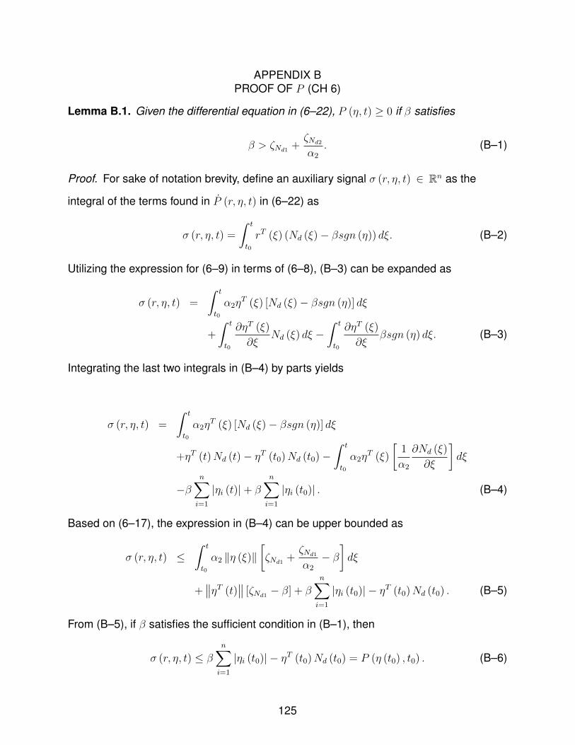
APPENDIX BPROOF OF P (CH 6)

Lemma B.1. Given the differential equation in (6–22), P (η, t) ≥ 0 if β satisfies

β > ζNd1+ζNd2

α2

. (B–1)

Proof. For sake of notation brevity, define an auxiliary signal σ (r, η, t) ∈ Rn as the

integral of the terms found in P (r, η, t) in (6–22) as

σ (r, η, t) =

ˆ t

t0

rT (ξ) (Nd (ξ)− βsgn (η)) dξ. (B–2)

Utilizing the expression for (6–9) in terms of (6–8), (B–3) can be expanded as

σ (r, η, t) =

ˆ t

t0

α2ηT (ξ) [Nd (ξ)− βsgn (η)] dξ

+

ˆ t

t0

∂ηT (ξ)

∂ξNd (ξ) dξ −

ˆ t

t0

∂ηT (ξ)

∂ξβsgn (η) dξ. (B–3)

Integrating the last two integrals in (B–4) by parts yields

σ (r, η, t) =

ˆ t

t0

α2ηT (ξ) [Nd (ξ)− βsgn (η)] dξ

+ηT (t)Nd (t)− ηT (t0)Nd (t0)−ˆ t

t0

α2ηT (ξ)

[1

α2

∂Nd (ξ)

∂ξ

]dξ

−βn∑i=1

|ηi (t)|+ βn∑i=1

|ηi (t0)| . (B–4)

Based on (6–17), the expression in (B–4) can be upper bounded as

σ (r, η, t) ≤ˆ t

t0

α2 ‖η (ξ)‖[ζNd1

+ζNd1

α2

− β]dξ

+∥∥ηT (t)

∥∥ [ζNd1− β] + β

n∑i=1

|ηi (t0)| − ηT (t0)Nd (t0) . (B–5)

From (B–5), if β satisfies the sufficient condition in (B–1), then

σ (r, η, t) ≤ βn∑i=1

|ηi (t0)| − ηT (t0)Nd (t0) = P (η (t0) , t0) . (B–6)

125

Integrating both sides of P (η (t0) , t0) in (6–22) yields

P (η, t) = P (η (t0) , t0)− σ (r, η, t)

which indicates that P (η, t) ≥ 0 from (B–6).

126

APPENDIX CPROOF OF χ BOUND (CH 7)

Lemma C.1. The MVT can be used to develop the upper bound in (7–15)

‖χ‖ ≤ χ (‖z‖) ‖z‖

where the bounding function χ : R4n+1 → R is a positive, globally invertible, nondecreas-

ing function, and z (e, ef , r, ez, P ) ∈ R4n+1 is defined as

z ,

[eT TanhT (ef ) rT eTz

√P

]T. (C–1)

Proof. The proof of Lemma C.1 follows from that of [164, App A]. The auxiliary error

χ (·) in (7–13) can be written as the sum of errors pertaining to each of its arguments as

follows:

χ (·) = χ (x, x, e, r, Tanh (ef ) , ez)− χ (xd, xd, 0, 0, 0, 0)

= χ (x, xd, 0, 0, 0, 0)− χ (xd, xd, 0, 0, 0, 0)

+χ (x, x, 0, 0, 0, 0)− χ (x, xd, 0, 0, 0, 0)

+χ (x, x, e, 0, 0, 0)− χ (x, x, 0, 0, 0, 0)

+χ (x, x, e, r, 0, 0)− χ (x, x, e, 0, 0, 0)

+χ (x, x, e, r, Tanh (ef ) , 0)− χ (x, x, e, r, 0, 0)

+χ (x, x, e, r, Tanh (ef ) , ez)− χ (x, x, e, r, Tanh (ef ) , 0) .

Applying the MVT to further describe χ (·),

χ (·) =∂χ (σ1, xd, 0, 0, 0, 0)

∂σ1

|σ1=v1 (x− xd) +∂χ (x, σ2, 0, 0, 0, 0)

∂σ2

|σ2=v2 (x− xd)

+∂χ (x, x, σ3, 0, 0, 0)

∂σ3

|σ3=v3 (e− 0) +∂χ (x, x, e, σ4, 0, 0)

∂σ4

|σ4=v4 (r − 0)

∂χ (x, x, e, r, σ4, 0)

∂σ5

|σ5=v5 (Tanh (ef )− 0)

+∂χ (x, x, e, r, Tanh (ef ) , σ5)

∂σ6

|σ6=v6 (ez − 0) (C–2)

127

where

v1 = x− c1 (x− xd) , v2 = x− c2 (x− xd) , v3 = e (1− c3) ,

v4 = r (1− c4) , v5 = ef (1− c5) , v6 = ez (1− c6)

and ci ∈ (0, 1) ∈ R, i = [1, 6] are unknown constants. From (C–2), χ (·) can be upper

bounded as

‖χ (·)‖ =

∥∥∥∥∂χ (σ1, xd, 0, 0, 0)

∂σ1

|σ1=v1

∥∥∥∥ ‖e‖+

∥∥∥∥∂χ (x, σ2, 0, 0, 0)

∂σ2

|σ2=v2

∥∥∥∥ ‖r − αTanh (e) + Tanh (ef )− ez‖

+

∥∥∥∥∂χ (x, x, σ3, 0, 0)

∂σ3

|σ3=v3

∥∥∥∥ ‖e‖+

∥∥∥∥∂χ (x, x, e, σ4, 0, 0)

∂σ4

|σ4=v4

∥∥∥∥ ‖r‖+

∥∥∥∥∂χ (x, x, e, r, σ4, 0)

∂σ5

|σ5=v5

∥∥∥∥ ‖Tanh (ef )‖

+

∥∥∥∥∂χ (x, x, e, r, Tanh (ef ) , σ5)

∂σ6

|σ6=v6

∥∥∥∥ ‖ez‖ . (C–3)

We can upper bound the partial derivatives as∥∥∥∥∂χ (σ1, xd, 0, 0, 0)

∂σ1

|σ1=v1

∥∥∥∥ ≤ ρ1 (e)∥∥∥∥∂χ (x, σ2, 0, 0, 0)

∂σ2

|σ2=v2

∥∥∥∥ ≤ ρ2 (r, e, Tanh (ef ) , ez)∥∥∥∥∂χ (x, x, σ3, 0, 0)

∂σ3

|σ3=v3

∥∥∥∥ ≤ ρ3 (e)∥∥∥∥∂χ (x, x, e, σ4, 0, 0)

∂σ4

|σ4=v4

∥∥∥∥ ≤ ρ4 (r)∥∥∥∥∂χ (x, x, e, r, σ4, 0)

∂σ5

|σ5=v5

∥∥∥∥ ≤ ρ5 (Tanh (ef ))∥∥∥∥∂χ (x, x, e, r, ef , σ5)

∂σ6

|σ6=v6

∥∥∥∥ ≤ ρ6 (ez)

where ρi (·) ∈ R, i = [1, 6] are positive, nondecreasing functions. The bound on χ (·) can

be further simplified

‖χ (·)‖ ≤ ρ1 (e) ‖e‖+ ρ2 (r, e, Tanh (ef ) , ez) ‖r − αTanh (e) + Tanh (ef )− ez‖

+ρ3 (e) ‖e‖+ ρ4 (r) ‖r‖+ ρ5 (Tanh (ef )) ‖Tanh (ef )‖+ ρ6 (ez) ‖ez‖ .

128

Since ‖Tanh (e)‖ ≤ ‖e‖ , the upper bound

‖r − αTanh (e) + Tanh (ef )− ez‖ ≤ ‖r‖+ α ‖e‖+ ‖Tanh (ef )‖+ ‖ez‖ ,

can be used to bound χ (·) as

‖χ (·)‖ ≤ (ρ1 (e) + ρ3 (e) + αρ2 (r, e, Tanh (ef ) , ez)) ‖e‖

+ (ρ2 (r, e, Tanh (ef ) , ez) + ρ4 (r)) ‖r‖

+ (ρ2 (r, e, Tanh (ef ) , ez) + ρ5 (Tanh (ef ))) ‖Tanh (ef )‖

+ (ρ2 (r, e, Tanh (ef ) , ez) + ρ6 (ez)) ‖ez‖ .

Using the definition from (C–1), χ (·) can be expressed in terms of z (·) as

‖χ (·)‖ ≤ (ρ1 (e) + ρ3 (e) + αρ2 (r, e, Tanh (ef ) , ez)) ‖z‖

+ (ρ2 (r, e, Tanh (ef ) , ez) + ρ4 (r)) ‖z‖

+ (ρ2 (r, e, Tanh (ef ) , ez) + ρ5 (Tanh (ef ))) ‖z‖

+ (ρ2 (r, e, Tanh (ef ) , ez) + ρ6 (ez)) ‖z‖ ,

‖χ (·)‖ ≤ (ρ1 + (α + 3) ρ2 + ρ3 + ρ4 + ρ5 + ρ6) ‖z‖ .

Therefore,

‖χ (·)‖ ≤ χ (‖z‖) ‖z‖

where χ (‖z‖) is some positive, nondecreasing function. Any positive nondecreasing

function can be upper bounded by a positive strictly increasing function. Thus, the

conditions for global invertibility hold. Finally,

‖χ (·)‖ ≤ χ (‖z‖) ‖z‖ ≤ χ (‖z‖) ‖z‖

where χ (‖z‖) is a positive globally invertible, nondecreasing function. Note that since√P is positive by definition, its conservative matter in the bounding of χ does not play a

factor.

129

REFERENCES

[1] Z. Qu, Robust Control of Nonlinear Uncertain Systems. Wiley Inc., New-York,1998.

[2] V. I. Utkin, Sliding Modes in Control and Optimization. Springer-Verlag, 1992.

[3] J. Slotine and W. Li, Applied Nonlinear Control. Prentice Hall, 1991.

[4] C. Abdallah, D. Dawson, P. Dorato, and M. Jamshidi, “Survey of robust control forrigid robots,” IEEE Control System Mag., vol. 11, no. 2, pp. 24–30, 1991.

[5] K. Zhou and J. C. Doyle, Essentials of Robust Control. Prentice Hall, 1997.

[6] A. Ilchmann and E. Ryan, “High-gain control without identification: A survey,”GAMM Mitt, vol. 31, no. 1, pp. 115–125, 2008.

[7] Y. Wang, L. Xie, and C. E. de Souza, “Robust control of a class of uncertainnonlinear systems,” Syst. Control Lett., vol. 19, pp. 139–149, August 1992.

[8] P. M. Patre, W. Mackunis, C. Makkar, and W. E. Dixon, “Asymptotic tracking forsystems with structured and unstructured uncertainties,” IEEE Trans. Control Syst.Technol., vol. 16, pp. 373–379, 2008.

[9] Z. Qu and J. X. Xu, “Model-based learning controls and their comparisons usinglyapunov direct method,” in Asian Journal of Control, vol. 4, No. 1, no. No. 1, Mar.2002, pp. 99–110.

[10] Z. Guo and L. Huang, “Generalized Lyapunov method for discontinuous systems,”Nonlinear Anal., vol. 71, pp. 3083–3092, 2009.

[11] G. Cheng and X. Mu, “Finite-time stability with respect to a closed invariant set fora class of discontinuous systems,” Appl. Math. Mech., vol. 30(8), pp. 1069–1075,2009.

[12] M. Forti, M. Grazzini, P. Nistri, and L. Pancioni, “Generalized Lyapunov approachfor convergence of neural networks with discontinuous or non-Lipschitz activations,”Physica D, vol. 214, pp. 88–99, 2006.

[13] Q. Wu and N. Sepehri, “On Lyapunov’s stability analysis of non-smooth systemswith applications to control engineering,” Int. J. of Nonlinear Mech., vol. 36, no. 7,pp. 1153–1161, 2001.

[14] Q. Wu, N. Sepehri, P. Sekhavat, and S. Peles, “On design of continuous Lyapunov’sfeedback control,” J. Franklin Inst., vol. 342, no. 6, pp. 702–723, 2005.

[15] E. Moulay and W. Perruquetti, “Finite time stability of differential inclusions,” IMA J.Math. Control Info., vol. 22, pp. 465–275, 2005.

130

[16] R. Sipahi, S.-I. Niculescu, C. Abdallah, W. Michiels, and K. Gu, “Stability andstabilization of systems with time delay: Limitations and opportunities,” IEEE Contr.Syst. Mag., vol. 31, no. 1, pp. 38–65, 2011.

[17] K. Gu and S. Niculescu, “Survey on recent results in the stability and control oftime-delay systems,” J. Dyn. Syst. Meas. Contr., vol. 125, p. 158, 2003.

[18] J.-P. Richard, “Time-delay systems: an overview of some recent advances andopen problems,” Automatica, vol. 39, no. 10, pp. 1667 – 1694, 2003.

[19] K. Watanabe, E. Nobuyama, and A. Kojima, “Recent advances in control of timedelay systems-a tutorial review,” in IEEE Conf. Decis. Control, vol. 2, 1996, pp.2083–2089.

[20] J. Chiasson and J. Loiseau, Applications of time delay systems, ser. Lecture notesin control and information sciences. Springer, 2007.

[21] K. Gu, V. L. Kharitonov, and J. Chen, Stability of Time-delay systems. Birkhauser,2003.

[22] M. Krstic, Delay Compensation for Nonlinear, Adaptive, and PDE Systems.Springer, 2009.

[23] J. Loiseau, W. Michiels, S.-I. Niculescu, and R. Sipahi, Eds., Topics in Time DelaySystems: Analysis, Algorithms, and Control. Spring Verlag, 2009.

[24] M. S. Mahmoud, Robust control and filtering for time-delay systems. CRC Press,2000.

[25] S.-I. Niculescu and K. Gu, Advances in time-delay systems. Spring Verlag, 2004.

[26] M. Krstic and A. Smyshlyaev, “Backstepping boundary control for first-orderhyperbolic PDEs and application to systems with actuator and sensor delays,”Syst. Contr. Lett., vol. 57, no. 9, pp. 750–758, 2008.

[27] D. Bresch-Pietri and M. Krstic, “Adaptive trajectory tracking despite unknown inputdelay and plant parameters,” Automatica, vol. 45, no. 9, pp. 2074 – 2081, 2009.

[28] F. Mazenc, S. Mondie, R. Francisco, P. Conge, I. Lorraine, and F. Metz, “Globalasymptotic stabilization of feedforward systems with delay in the input,” IEEETrans. Autom. Control, vol. 49, (5), pp. 844–850, 2004.

[29] B. Chen, X. Liu, and S. Tong, “Robust fuzzy control of nonlinear systems with inputdelay,” Chaos, Solitons & Fractals, vol. 37, no. 3, pp. 894–901, 2008.

[30] M. Krstic, “Input delay compensation for forward complete and strict-feedforwardnonlinear systems,” IEEE Trans. Autom. Control, vol. 55, pp. 287–303, feb. 2010.

131

[31] N. Sharma, S. Bhasin, Q. Wang, and W. E. Dixon, “Predictor-based control for anuncertain Euler-Lagrange system with input delay,” Automatica, vol. 47, no. 11, pp.2332–2342, 2011.

[32] B. Castillo-Toledo, S. Di Gennaro, and G. Castro, “Stability analisys for a class ofsampled nonlinear systems with time-delay,” in Proc. IEEE Conf. Decis. Control,2010, pp. 1575 –1580.

[33] A. Bacciotti and L. Rosier, Liapunov functions and stabilty in control theory.Springer, 2005.

[34] V. M. Matrosov, “On the stability of motion,” J. Appl. Math. Mech., vol. 26, pp.1337–1353, 1962.

[35] A. Loría, E. Panteley, D. Popovic, and A. R. Teel, “A nested Matrosov theoremand persistency of excitation for uniform convergence in stable nonautonomoussystems,” IEEE Trans. Autom. Contr., vol. 50, no. 2, pp. 183–198, 2005.

[36] R. Sanfelice and A. Teel, “Asymptotic stability in hybrid systems via nestedMatrosov functions,” IEEE Trans. on Autom. Control, vol. 54, no. 7, pp. 1569–1574,July 2009.

[37] M. Malisoff and F. Mazenc, “Constructions of strict Lyapunov functions for discretetime and hybrid time-varying systems,” Nonlin. Anal.: Hybrid Syst., vol. 2, no. 2, pp.394–407, 2008.

[38] A. Teel, E. Panteley, and A. Loría, “Integral characterizations of uniform asymptoticand exponential stability with applications,” Math. of Control, Signals, and Sys.,vol. 15, pp. 177–201, 2002.

[39] A. Astolfi and L. Praly, “A LaSalle version of Matrosov theorem,” in Proc. IEEEConf. Decis. Control, 2011, pp. 320–324.

[40] J. P. LaSalle, An Invariance Principle in the Theory of Stability. New York:Academic Press, 1967.

[41] C. Byrnes and C. Martin, “An integral-invariance principle for nonlinear systems,”IEEE Trans. on Autom. Control, vol. 40, no. 6, pp. 983–994, 1995.

[42] E. Ryan, “An integral invariance principle for differential inclusions with applicationsin adaptive control,” SIAM J. Control Optim., vol. 36, no. 3, pp. 960–980, 1998.

[43] R. Sanfelice, R. Goebel, and A. Teel, “Invariance principles for hybrid systems withconnections to detectability and asymptotic stability,” IEEE Trans. Autom. Contr.,vol. 52, no. 12, pp. 2282–2297, 2007.

[44] H. Logemann and E. Ryan, “Asymptotic behaviour of nonlinear systems,” Amer.Math. Month., vol. 111, pp. 864–889, 2004.

132

[45] D. Shevitz and B. Paden, “Lyapunov stability theory of nonsmooth systems,” IEEETrans. Autom. Control, vol. 39 no. 9, pp. 1910–1914, 1994.

[46] A. Bacciotti and F. Ceragioli, “Stability and stabilization of discontinuous systemsand nonsmooth Lyapunov functions,” Control, Optim., and Calc. of Var., vol. 4, pp.361–376, 1999.

[47] ——, “Nonpathological Lyapunov functions and discontinuous Caratheodorysystems,” Automatica, vol. 42, pp. 453–458, 2006.

[48] J. Hespanha, “Uniform stability of switched linear systems: Extensions of LaSalle’sInvariance Principle,” IEEE Trans. on Autom. Control, vol. 49, no. 4, pp. 470–482,April 2004.

[49] V. Chellaboina, S. Bhat, and W. Haddad, “An invariance principle for nonlinearhybrid and impulsive dynamical systems,” Nonlinear Anal., vol. 53, pp. 527–550,2003.

[50] J. Lygeros, K. Johansson, J. Simic, Z. Jiang, and S. Sastry, “Dynamical propertiesof hybrid automata,” IEEE Trans. on Autom. Control, vol. 48, no. 1, pp. 2–17, Jan.2003.

[51] J. Hespanha, D. Liberzon, D. Angeli, and E. Sontag, “Nonlinear norm-observabilitynotions and stability of switched systems,” IEEE Trans. on Autom. Control, vol. 50,no. 2, pp. 154–168, Feb. 2005.

[52] A. Bacciotti and L. Mazzi, “An invariance principle for nonlinear switched systems,”Syst. Contr. Lett., vol. 54, pp. 1109–1119, 2005.

[53] R. Goebel, R. Sanfelice, and A. Teel, Hybrid Dynamical Systems. PrincetonUniversity Press, 2012.

[54] T.-C. Lee, D.-C. Liaw, and B.-S. Chen, “A general invariance principle for nonlineartime-varying systems and its applications,” IEEE Trans. Autom. Contr., vol. 46,no. 12, pp. 1989 –1993, dec 2001.

[55] H. K. Khalil, Nonlinear Systems, 3rd ed. Prentice Hall, 2002.

[56] F. Clarke, Optimization and Nonsmooth Analysis. Reading, MA: Addison-Wesley,1983.

[57] V. V. Nemyckii and V. V. Stepanov, Qualitative theory of differential equations.Princeton Univ. Press, N.J., 1960.

[58] C. M. Kellett and A. R. Teel, “Weak converse Lyapunov theorems and controlLyapunov functions,” SIAM J. Contr. Optim., vol. 42, no. 6, pp. 1934–1959, 2004.

133

[59] A. R. Teel and L. Praly, “A smooth Lyapunov function from a class-KL estimateinvolving two positive semidefinite functions,” ESAIM Contr. Optim. Calc. Var.,vol. 5, pp. 313–367, 2000.

[60] I. Moise, R. Rosa, and X. Wang, “Attractors for noncompact nonautonomoussystems via energy equations,” Discret. Contin. Dyn. Syst., vol. 10, pp. 473–496,2004.

[61] T. Caraballo, G. Åukaszewicz, and J. Real, “Pullback attractors for asymptoticallycompact non-autonomous dynamical systems,” Nonlin. Anal.: Theory, Methods,Appl., vol. 64, no. 3, pp. 484 – 498, 2006.

[62] G. R. Sell, “Nonautonomous differential equations and topological dynamics i. thebasic theory,” Trans. Amer. Math. Society, vol. 127, no. 2, pp. 241–262, 1967.

[63] M. Vidyasagar, Nonlinear Systems Analysis, 2nd ed. SIAM, 2002.

[64] T.-C. Lee and Z.-P. Jiang, “A generalization of Krasovskii-LaSalle theorem fornonlinear time-varying systems: Converse results and applications,” IEEE Trans.Autom. Contr., vol. 50, no. 8, pp. 1147–1163, 2005.

[65] Z. Artstein, “Uniform asymptotic stability via the limiting equations,” J. Diff. Equat.,vol. 27, pp. 172–189, 1978.

[66] J. Alvarez, Y. Orlov, and L. Acho, “An invariance principle for discontinuousdynamic systems with applications to a Coulomb friction oscillator,” ASME J.Dynam. Syst., Meas., Control, vol. 74, pp. 190–198, 2000.

[67] Y. Orlov, “Extended invariance principle for nonautonomous switched systems,”IEEE Trans. Autom. Contr., vol. 48, no. 8, pp. 1448–1452, 2003.

[68] M. Krstic, P. V. Kokotovic, and I. Kanellakopoulos, Nonlinear and Adaptive ControlDesign. John Wiley & Sons, 1995.

[69] J. P. LaSalle, “Some extensions of Liapunov’s second method,” IRE Trans. CircuitTheory, vol. CT-7, pp. 520–527, 1960.

[70] T. Yoshizawa, “Asymptotic behavior of solutions of a system of differentialequations,” Contrib. Differ. Equ., vol. 1, pp. 371–387, 1963.

[71] A. Teel, “Asymptotic convergence from lp stability,” IEEE Trans. Autom. Contr.,vol. 44, no. 11, pp. 2169–2170, 1999.

[72] R. Colbaugh, E. Barany, and K. Glass, “Global regulation of uncertain manipulatorsusing bounded controls,” in Proc. IEEE Int. Conf. Robot. Autom., vol. 2, 1997, pp.1148–1155.

134

[73] R. Kelly and V. Santibanez, “A class of global regulators with bounded controlactions for robot manipulators,” in Proc. IEEE Conf. Decis. Control, vol. 3, 1996,pp. 3382–3387.

[74] A. Zavala-Rio and V. Santibanez, “A natural saturating extension of the PD-with-desired-gravity-compensation control law for robot manipulators with boundedinputs,” IEEE Trans. Robot., vol. 23, no. 2, pp. 386–391, 2007.

[75] H. Yazarel, C. C. Cheah, and H. C. Liaw, “Adaptive SP-D control of a roboticmanipulator in the presence of modeling error in a gravity regressor matrix: theoryand experiment,” IEEE Trans. Robot. Autom., vol. 18, no. 3, pp. 373–379, 2002.

[76] Y. X. Su, D. Sun, L. Ren, and J. Mills, “Integration of saturated PI synchronouscontrol and PD feedback for control of parallel manipulators,” IEEE Trans. Robot,vol. 22(1), pp. 202–207, 2006.

[77] V. Santibanez, R. Kelly, and M. Llama, “A novel global asymptotic stable set-pointfuzzy controller with bounded torques for robot manipulators,” IEEE Trans. FuzzySyst., vol. 13, no. 3, pp. 362–372, 2005.

[78] W. E. Dixon, D. M. Dawson, F. Zhang, and E. Zergeroglu, “Global exponentialtracking control of a mobile robot system via a pe condition,” in Proc. IEEE Conf.Decis. Control, Phoenix, Arizona, December 1999, pp. 4822–4827.

[79] E. Aguinaga-Ruiz, A. Zavala-Rio, V. Santibanez, and F. Reyes, “Global trajectorytracking through static feedback for robot manipulators with bounded inputs,” IEEETrans. Control Syst. Technol., vol. 17, no. 4, pp. 934–944, 2009.

[80] V. Santibanez and R. Kelly, “Global asymptotic stability of bounded output feedbacktracking control for robot manipulators,” in Proc. IEEE Conf. Decis. Control, vol. 2,2001, pp. 1378–1379.

[81] J. Moreno-Valenzuela, V. Santibáñez, and R. Campa, “A class of OFT controllersfor torque-saturated robot manipulators: Lyapunov stability and experimentalevaluation,” J. Intell. Rob. Syst., vol. 51, pp. 65–88, 2008.

[82] A. Loria and H. Nijmeijer, “Bounded output feedback tracking control of fullyactuated Euler-Lagrange systems,” Syst. Control Lett., vol. 33, pp. 151–161, March1998.

[83] J. Alvarez-Ramirez, V. Santibanez, and R. Campa, “Stability of robot manipulatorsunder saturated PID compensation,” IEEE Trans. Control Syst. Technol., vol. 16,no. 6, pp. 1333–1341, Nov. 2008.

[84] Y. Su, P. Muller, and C. Zheng, “Global asymptotic saturated PID control for robotmanipulators,” IEEE Trans. Control Syst. Technol., vol. 18, no. 6, pp. 1280–1288,2010.

135

[85] Y. Hong and B. Yao, “A globally stable high-performance adaptive robust controlalgorithm with input saturation for precision motion control of linear motor drivesystems,” IEEE/ASME Trans. Mechatron., vol. 12, no. 2, pp. 198–207, 2007.

[86] M. Corradini, A. Cristofaro, and G. Orlando, “Robust stabilization of multi inputplants with saturating actuators,” IEEE Trans. Autom. Control, vol. 55, no. 2, pp.419–425, 2010.

[87] J. D. Boskovic, S.-M. Li, and R. K. Mehra, “Robust adaptive variable structurecontrol of spacecraft under control input saturation,” J. Guid. Contr. Dynam., vol.24(1), pp. 14–22, 2001.

[88] L. Zhang, J. Xie, and D. Lu, “Adaptive robust control of one-link joint actuatedby pneumatic artificial muscles,” in Proc. Conf. BioInfo. Biomed. Eng., 2007, pp.1185–1189.

[89] F. Morabito, A. Teel, and L. Zaccarian, “Nonlinear antiwindup applied to Euler-Lagrange systems,” Robotics and Automation, IEEE Transactions on, vol. 20,no. 3, pp. 526–537, 2004.

[90] R. Gorez, “Globally stable PID-like control of mechanical systems.” Syst. Contr.Lett., vol. 38, pp. 61–72, 1999.

[91] J. L. Meza, V. Santibanez, and V. Hernandez, “Saturated nonlinear PID globalregulator for robot manipulators: Passivity based analysis,” in Proc. IFAC WorldCongr., Prague, Czech Republic, 2005.

[92] M. Arcak, A. Teel, and P. Kokotovic, “Robust nonlinear control of feedforwardsystems with unmodeled dynamics,” Automatica, vol. 37, no. 2, pp. 265–272, 2001.

[93] L. Marconi and A. Isidori, “Robust global stabilization of a class of uncertainfeedforward nonlinear systems,” Systems & Control Letters, vol. 41, no. 4, pp.281–290, 2000.

[94] G. Kaliora and A. Astolfi, “Nonlinear control of feedforward systems with boundedsignals,” Automatic Control, IEEE Transactions on, vol. 49, no. 11, pp. 1975–1990,2004.

[95] S. S. Ge, F. Hong, and T. H. Lee, “Adaptive neural control of nonlinear time-delaysystems with unknown virtual control coefficients,” IEEE Trans. Syst. Man Cybern.Part B Cybern., vol. 34, no. 1, pp. 499–516, 2004.

[96] S. Ge, F. Hong, and T. Lee, “Robust adaptive control of nonlinear systems withunknown time delays,” Automatica, vol. 41, no. 7, pp. 1181–1190, Jul. 2005.

[97] S. J. Yoo, J. B. Park, and C. H. Choi, “Adaptive dynamic surface control forstabilization of parametric strict-feedback nonlinear systems with unknown timedelays,” IEEE Trans. Autom. Contr., vol. 52, no. 12, pp. 2360–2365, 2007.

136

[98] C.-C. Hua, X.-P. Guan, and G. Feng, “Robust stabilisation for a class of time-delaysystems with triangular structure,” IET Control Theory Appl., vol. 1, no. 4, pp.875–879, 2007.

[99] H. Wu, “Adaptive robust state observers for a class of uncertain nonlineardynamical systems with delayed state perturbations,” IEEE Trans. Automat. Contr.,vol. 54, no. 6, pp. 1407–1412, 2009.

[100] M. Wang, B. Chen, and S. Zhang, “Adaptive neural tracking control of nonlineartime-delay systems with disturbances,” Int. J. Adapt Control Signal Process.,vol. 23, pp. 1031–1049, 2009.

[101] S.-C. Tong and N. Sheng, “Adaptive fuzzy observer backstepping control for aclass of uncertain nonlinear systems with unknown time-delay,” Int.. J. Autom. andComput., vol. 7, no. 2, pp. 236–246, 2010.

[102] A. Kuperman and Q.-C. Zhong, “Robust control of uncertain nonlinear systemswith state delays based on an uncertainty and disturbance estimator,” Int. J. RobustNonlinear Control, vol. 21, pp. 79–92, 2011.

[103] Z. Wang and K. J. Burnham, “Robust filtering for a class of stochastic uncertainnonlinear time-delay systems via exponential state estimation,” IEEE Trans. SignalProcess., vol. 49, no. 4, pp. 794–804, 2001.

[104] H. Huang and D. Ho, “Delay-dependent robust control of uncertain stochasticfuzzy systems with time-varying delay,” IET Control Theory Appl., vol. 1, no. 4, pp.1075–1085, 2007.

[105] B. Ren, S. S. Ge, T. H. Lee, and C. Su, “Adaptive neural control for a class ofnonlinear systems with uncertain hysteresis inputs and time-varying state delays,”IEEE Trans. Neural Netw., vol. 20, pp. 1148–1164, 2009.

[106] S. J. Yoo and J. B. Park, “Neural-network-based decentralized adaptive control fora class of large-scale nonlinear systems with unknown time-varying delays,” IEEETrans. Syst. Man Cybern., vol. 39, no. 5, pp. 1316–1323, 2009.

[107] M. Wang, S. S. Ge, and K. Hong, “Approximation-based adaptive tracking controlof pure-feedback nonlinear systems with multiple unknown time-varying delays,”IEEE Trans. Neur. Netw., vol. 21, no. 11, pp. 1804–1816, 2010.

[108] Y. Niu, D. W. C. Ho, and J. Lam, “Robust integral sliding mode control for uncertainstochastic systems with time-varying delay,” Automatica, vol. 41, pp. 873–880,2005.

[109] T. Zhang, Q. Wang, H. Wen, and Y. Yang, “Adaptive fuzzy control for a class ofnonlinear time-varying delay systems,” in Proc. World Congr. Intell. Control andAutom., Chongqing, China, 2008.

137

[110] W. Chen, L. Jiao, J. Li, and R. Li, “Adaptive nn backstepping output-feedbackcontrol for stochastic nonlinear strict-feedback systems with time-varying delays,”IEEE Trans. Syst. Man Cybern., vol. 40, no. 3, pp. 939–950, 2010.

[111] B. Mirkin and P.-O. Gutman, “Robust adaptive output-feedback tracking for a classof nonlinear time-delayed plants,” IEEE Trans. Automat. Contr., vol. 55, no. 10, pp.2418–2424, 2010.

[112] B. Mirkin, P.-O. Gutman, Y. Shtessel, and C. Edwards, “Continuous decentralizedMRAC with sliding mode of nonlinear delayed dynamic systems,” in IFAC WorldCongr., Milano, Italy, 2011.

[113] O. M. Smith, “A controller to overcome deadtime,” ISA J., vol. 6, pp. 28–33, 1959.

[114] Z. Artstein, “Linear systems with delayed controls: A reduction,” IEEE Trans.Autom. Control, vol. 27, no. 4, pp. 869–879, 1982.

[115] A. Manitius and A. Olbrot, “Finite spectrum assignment problem for systems withdelays,” IEEE Trans. Autom. Control, vol. 24, no. 4, pp. 541–552, 1979.

[116] M. Nihtila, “Adaptive control of a continuous-time system with time-varying inputdelay,” IEEE Trans. Autom. Contr., vol. 12, pp. 357–364, 1989.

[117] ——, “Finite pole assignment for systems with time-varying input delays,” in Proc.IEEE Conf. Decis. Control, 1991, pp. 927–928.

[118] R. Lozano, P. Castillo, P. Garcia, and A. Dzul, “Robust prediction-based controlfor unstable delay systems: Application to the yaw control of a mini-helicopter,”Automatica, vol. 40, no. 4, pp. 603–612, 2004.

[119] D. Yue and Q.-L. Han, “Delayed feedback control of uncertain systems withtime-varying input delay,” Automatica, vol. 41, no. 2, pp. 233–240, 2005.

[120] Z. Wang, P. Goldsmith, and D. Tan, “Improvement on robust control of uncertainsystems with time-varying input delays,” IET Control Theory Appl., vol. 1, no. 1, pp.189 –194, 2007.

[121] M. Krstic, “Lyapunov stability of linear predictor feedback for time-varying inputdelay,” IEEE Trans. Autom. Control, vol. 55, pp. 554–559, 2010.

[122] N. Sharma, S. Bhasin, Q. Wang, and W. E. Dixon, “RISE-based adaptive controlof a control affine uncertain nonlinear system with unknown state delays,” IEEETrans. Automat. Control, vol. 57, no. 1, pp. 255–259, Jan. 2012.

[123] N. Fischer, R. Kamalapurkar, N. Sharma, and W. E. Dixon, “Rise-based control ofan uncertain nonlinear system with time-varying state delays,” in Proc. IEEE Conf.Decis. Control, Maui, HI, Dec. 2012.

138

[124] F. Mazenc and S.-I. Niculescu, “Generating positive and stable solutions throughdelayed state feedback,” Automatica, vol. 47, pp. 525–533, 2011.

[125] I. Karafyllis, “Stabilization by means of approximate predictors for systems withdelayed input,” SIAM J. Control Optim., vol. 49, no. 3, pp. 1100–1123, 2011.

[126] F. Carravetta, P. Palumbo, and P. Pepe, “Quadratic optimal control of linearsystems with time-varying input delay,” in Proc. IEEE Conf. Decis. Contr., 2010, pp.4996–5000.

[127] F. Mazenc, S. Niculescu, and M. Bekaik, “Stabilization of time-varying nonlinearsystems with distributed input delay by feedback of plant’s state,” AutomaticControl, IEEE Transactions on, vol. PP, no. 99, p. 1, 2012.

[128] P. Pepe, Z.-P. Jiang, and E. Fridman, “A new Lyapunov-Krasovskii methodologyfor coupled delay differential and difference equations,” Int. J. Control, vol. 81, pp.107–115, 2008.

[129] S. Obuz, E. Tatlicioglu, S. C. Cekic, and D. M. Dawson, “Predictor-based robustcontrol of uncertain nonlinear systems subject to input delay,” in IFAC Workshopon Time Delay Syst., vol. 10, no. 1, 2012.

[130] X. Jiao, J. Yang, and Q. Li, “Adaptive control for a class of nonlinear systemswith time-varying delays in the state and input,” J. Contr. Theory Appl., vol. 9, pp.183–188, 2011.

[131] J. Liu, J. Zhang, Y. Zheng, and M. He, “Robust H-infinity control for discrete-timeT-S fuzzy systems with input delay,” J. Contr. Theory Appl., vol. 9, pp. 189–194,2011.

[132] I. Karafyllis, “Finite-time global stabilization by means of time-varying distributeddelay feedback,” SIAM J. Control Optim., vol. 45, pp. 320–342, 2006.

[133] N. Bekiaris-Liberis and M. Krstic, “Compensation of time-varying input delay fornonlinear systems,” in Mediterr. Conf. Control and Autom., Corfu, Greece, 2011.

[134] ——, “Compensation of time-varying input and state delays for nonlinear systems,”J. Dyn. Syst. Meas. Contr., vol. 134, no. 1, p. 011009, 2012.

[135] ——, “Stabilization of linear strict feedback systems with delayed integrators,”Automatica, vol. 46, pp. 1902–1910, 2010.

[136] M. Jankovic, “Forwarding, backstepping, and finite spectrum assignment for timedelay systems,” Automatica, vol. 45, pp. 2–9, 2009.

[137] ——, “Recursive predictor design for state and output feedback controllers forlinear time delay systems,” Automatica, vol. 46, pp. 510–517, 2010.

139

[138] S. Tarbouriech and M. Turner, “Anti-windup design: an overview of some recentadvances and open problems,” IET Control Theory Appl., vol. 3, no. 1, pp. 1–19,2009.

[139] S.-I. Niculescu, J.-M. Dion, and L. Dugard, “Robust stabilization for uncertaintime-delay systems containing saturating actuators,” IEEE Trans. Autom. Control,vol. 41, no. 5, pp. 742–747, May 1996.

[140] H. Wang, Y. Wang, Y. Mao, Y. Jing, and L. Guo, “Robust congestion control foruncertain time-varying delay network systems,” in Proc. Conf. Chinese. ControlDecis., 2008, pp. 739–743.

[141] Y.-Y. Cao, Z. Wang, and J. Tang, “Analysis and anti-windup design for time-delaysystems subject to input saturation,” in Proc. Int. Conf. Mechatron. Autom., 2007,pp. 1968–1973.

[142] X. Cai, J. Huang, and L. Liu, “Stability analysis of linear time-delay differentialinclusion systems subject to input saturation,” IET Control Theory Appl., vol. 4,no. 11, pp. 2592–2602, 2010.

[143] J.-K. Park, C.-H. Choi, and H. Choo, “Dynamic anti-windup method for a class oftime-delay control systems with input saturation,” Int. J. Robust Nonlinear Control,vol. 10, no. 6, pp. 457–488, 2000.

[144] B. Zhou, Z. Lin, and G. Duan, “Stabilization of linear systems with input delay andsaturation - a parametric Lyapunov equation approach,” Int. J. Robust NonlinearControl, vol. 20, no. 13, pp. 1502–1519, 2010.

[145] Z. Bin and L. Zongli, “A parametric Lyapunov equation approach to stabilizationof discrete-time systems with input delay and saturation,” in Proc. Chinese ControlConf., 2010, pp. 5964–5969.

[146] F. Mazenc, S. Mondie, S. Niculescu, P. Conge, I. Lorraine, and F. Metz, “Globalasymptotic stabilization for chains of integrators with a delay in the input,” IEEETrans. Autom. Control, vol. 48, pp. 57–63, 2003.

[147] P. M. Patre, W. MacKunis, K. Kaiser, and W. E. Dixon, “Asymptotic tracking foruncertain dynamic systems via a multilayer neural network feedforward and RISEfeedback control structure,” IEEE Trans. Automat. Control, vol. 53, no. 9, pp.2180–2185, 2008.

[148] H. K. Khalil, Nonlinear Systems, 2nd ed. Prentice Hall, 1996.

[149] A. F. Filippov, Differential Equations with Discontinuous Right-hand Sides. KluwerAcademic Publishers, 1988.

[150] N. N. Krasovskii, Stability of motion. Stanford University Press, 1963.

[151] J. P. Aubin and A. Cellina, Differential Inclusions. Springer, Berlin, 1984.

140

[152] O. Hájek, “Discontinuous differential equations,” J. Diff. Eq., vol. 32, pp. 149–170,1979.

[153] F. M. Ceragioli, “Discontinuous ordinary differential equations and stabilization,”Ph.D. dissertation, Universita di Firenze, Italy, 1999.

[154] B. Paden and S. Sastry, “A calculus for computing Filippov’s differential inclusionwith application to the variable structure control of robot manipulators,” IEEE Trans.Circuits Syst., vol. 34 no. 1, pp. 73–82, 1987.

[155] W. Kaplan, Advanced Calculus, 4th ed. Reading, MA: Addison-Wesley, 1991.

[156] F. Clarke, Y. Ledyaev, R. Stern, and P. Wolenski, Nonsmooth Analysis and ControlTheory, 178th ed., ser. Graduate Texts in Mathematics. Springer, New York,1998.

[157] H. Hermes, “Discontinuous vector fields and feedback control,” in DifferentialEquations and Dynamical Systems. Academic Press, 1967.

[158] J.-M. Coron and L. Rosier, “A relation between continuous time-varying anddiscontinuous feedback stabilization,” J. Math. Systems. Estim. Control, vol. 4,no. 1, pp. 67–84, 1994.

[159] R. Goebel, R. Sanfelice, and A. Teel, “Hybrid dynamical systems,” IEEE Contr.Syst. Mag.,, vol. 29, no. 2, pp. 28 –93, 2009.

[160] B. Xian, D. M. Dawson, M. S. de Queiroz, and J. Chen, “A continuous asymptotictracking control strategy for uncertain nonlinear systems,” IEEE Trans. Autom.Control, vol. 49, pp. 1206–1211, 2004.

[161] A. Filippov, “Differential equations with discontinuous right-hand side,” Am. Math.Soc. Transl., vol. 42 no. 2, pp. 199–231, 1964.

[162] G. V. Smirnov, Introduction to the theory of differential inclusions. AmericanMathematical Society, 2002.

[163] J. P. Aubin and H. Frankowska, Set-valued analysis. Birkhäuser, 2008.

[164] M. de Queiroz, J. Hu, D. Dawson, T. Burg, and S. Donepudi, “Adaptiveposition/force control of robot manipulators without velocity measurements:Theory and experimentation,” IEEE Trans. Syst. Man Cybern., vol. 27-B, no. 5, pp.796–809, 1997.

[165] P. Patre, “Lyapunov-based robust and adaptive control of nonlinear systemsusing a novel feedback structure,” Ph.D. dissertation, University of Florida, 2009,available online: http://ncr.mae.ufl.edu/dissertations/patre.pdf.

[166] F. H. Clarke, Optimization and nonsmooth analysis. SIAM, 1990.

141

[167] R. Leine and N. van de Wouw, “Non-smooth dynamical systems,” in Stabilityand Convergence of Mechanical Systems with Unilateral Constraints, ser. LectureNotes in Applied and Computational Mechanics. Springer Berlin / Heidelberg,2008, vol. 36, pp. 59–77.

[168] P. Patre, W. Mackunis, K. Dupree, and W. E. Dixon, “Modular adaptive controlof uncertain Euler-Lagrange systems with additive disturbances,” IEEE Trans.Automat. Control, vol. 56, no. 1, pp. 155–160, 2011.

[169] C. Makkar, G. Hu, W. G. Sawyer, and W. E. Dixon, “Lyapunov-based trackingcontrol in the presence of uncertain nonlinear parameterizable friction,” IEEETrans. Automat. Control, vol. 52, pp. 1988–1994, 2007.

[170] C. Makkar, W. E. Dixon, W. G. Sawyer, and G.H, “A new continuously differentiablefriction model for control systems design,” in Proc. IEEE/ASME Int. Conf. Adv.Intell. Mechatron., Monterey, CA, July 2005, pp. 600–605.

[171] P. M. Patre, W. MacKunis, K. Dupree, and W. E. Dixon, RISE-Based Robust andAdaptive Control of Nonlinear Systems. Birkhäuser: Boston, 2010.

[172] N. Fischer, Z. Kan, and W. E. Dixon, “Saturated RISE feedback control forEuler-Lagrange systems,” in American Control Conference, Montréal, Canada,June 2012, pp. 244–249.

[173] K. S. Walgama, S. Ronnback, and J. Sternby, “Generalization of conditioningtechnique for anti-windup compensators,” Proc. IEE Control Theory Appl., vol. 139,no. 2, pp. 109–118, 1992.

[174] W. E. Dixon, M. S. de Queiroz, D. M. Dawson, and F. Zhang, “Tracking control ofrobot manipulators with bounded torque inputs,” Robotica, vol. 17, pp. 121–129,1999.

[175] T. Burg, D. M. Dawson, and P. Vedagarbha, “A redesigned dcal controller withoutvelocity measurements: Theory and demonstration,” Robotica, vol. 15, no. 4, pp.337–346, 1997.

[176] F. L. Lewis, R. Selmic, and J. Campos, Neuro-Fuzzy Control of Industrial Systemswith Actuator Nonlinearities. Philadelphia, PA, USA: Society for Industrial andApplied Mathematics, 2002.

[177] S. Bhasin, N. Sharma, P. Patre, and W. E. Dixon, “Asymptotic tracking by areinforcement learning-based adaptive critic controller,” J. of Control Theory andApp., vol. 9, no. 3, pp. 400–409, 2011.

[178] R. Francisco, F. Mazenc, and S. Mondié, Global asymptotic stabilization of aPVTOL aircraft model with delay in the input. Springer, 2007.

[179] F. Mazenc and S. Bowong, “Tracking trajectories of the cart-pendulum system,”Automatica, vol. 39, no. 4, pp. 677–684, 2003.

142

[180] N. Sharma, S. Bhasin, Q. Wang, and W. E. Dixon, “Predictor-based control foran uncertain Euler-Lagrange system with input delay,” in Proc. Am. Control Conf.,2010, pp. 1422–1427.

[181] N. Fischer, R. Kamalapurkar, N. Fitz-Coy, and W. E. Dixon, “Lyapunov-basedcontrol of an uncertain Euler-Lagrange system with time-varying input delay,” inAmerican Control Conference, Montréal, Canada, June 2012, pp. 3919–3924.

[182] N. Fischer, R. Kamalapurkar, and W. E. Dixon. (2012) A corollary for nonsmoothsystems. arXiv:1205.6765.

[183] F. Zhang, D. M. Dawson, M. S. de Queiroz, and W. E. Dixon, “Global adaptiveoutput feedback tracking control of robot manipulators,” IEEE Trans. Automat.Control, vol. 45, pp. 1203–1208, 2000.

[184] M. Corless and G. Leitmann, “Continuous state feedback guaranteeing uniformultimate boundedness for uncertain dynamic systems,” IEEE Trans. Autom.Control, vol. 26, no. 5, pp. 1139–1144, 1981.

[185] N. Fischer, A. Dani, N. Sharma, and W. E. Dixon, “Saturated control of anuncertain Euler-Lagrange system with input delay,” in Proc. IEEE Conf. Decis.Control, Orlando, FL, 2011, pp. 7587–7592.

143

BIOGRAPHICAL SKETCH

Nic Fischer was born in St. Petersburg, Florida. He received a Bachelor of Science

degree in mechanical engineering from the University of Florida in 2008. He joined

the Nonlinear Controls and Robotics (NCR) research group in 2006 with the hopes of

continuing his research into graduate school. After competing his bachelor’s degree,

Nic decided to pursue doctoral research in under the advisement of Dr. Warren Dixon

at the University of Florida. Focusing on nonlinear control theory and applications, Nic

earned a Master of Science degree in December of 2010 and completed his Ph.D. in

December of 2012, both in mechanical engineering. As a graduate researcher, Nic was

awarded the Outstanding Graduate Research Award for the Department of Mechanical

and Aerospace Engineering for his work in nonlinear control theory in 2012. He also

received the Ph.D. Gator Engineering Attribute of Professional Excellence award in 2012

from the UF College of Engineering. Nic has led several student projects including UF’s

SubjuGator autonomous underwater vehicle. Additionally, Nic worked as a mechanical

engineering intern at Honeywell International in 2006.

144