4. Lyapunov Stability 전자전기공학부 장석규 4.4 Comparison Functions ~ 4.9 Input-to-State Stability 1

Welcome message from author
This document is posted to help you gain knowledge. Please leave a comment to let me know what you think about it! Share it to your friends and learn new things together.
Transcript

4. Lyapunov Stability
전자전기공학부장석규
4.4 Comparison Functions~ 4.9 Input-to-State Stability
1
4.4 Comparison Functions
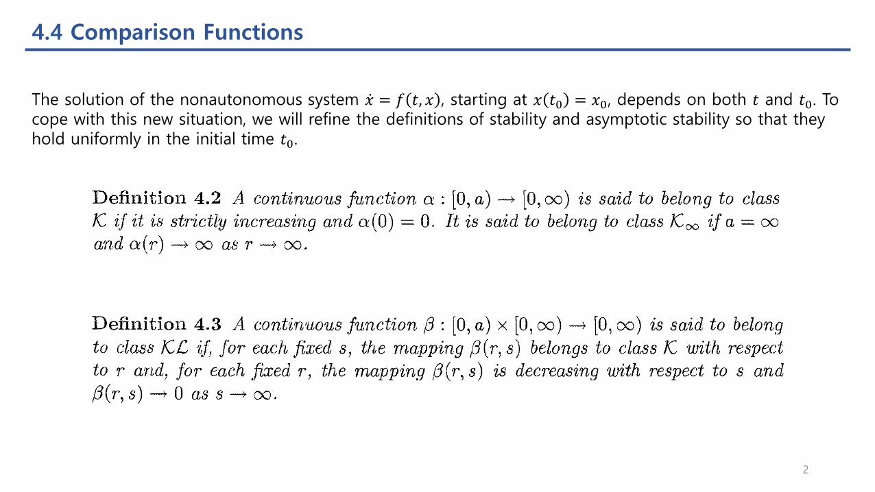
The solution of the nonautonomous system ሶ𝑥 = 𝑓 𝑡, 𝑥 , starting at 𝑥 𝑡0 = 𝑥0, depends on both 𝑡 and 𝑡0. To cope with this new situation, we will refine the definitions of stability and asymptotic stability so that they hold uniformly in the initial time 𝑡0.
2
4.4 Comparison Functions
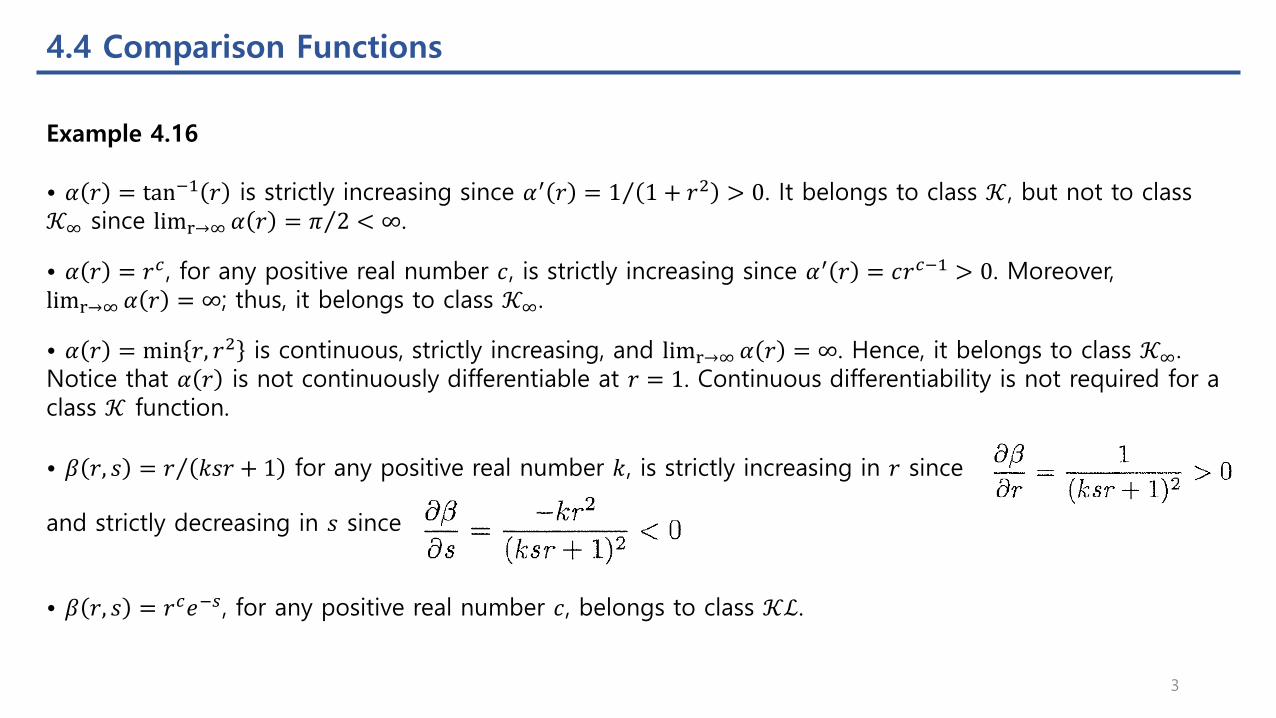
Example 4.16
• 𝛼 𝑟 = tan−1 𝑟 is strictly increasing since 𝛼′ 𝑟 = Τ1 1 + 𝑟2 > 0. It belongs to class 𝒦, but not to class 𝒦∞ since limr→∞ 𝛼 𝑟 = Τ𝜋 2 < ∞.
• 𝛼 𝑟 = 𝑟𝑐 , for any positive real number 𝑐, is strictly increasing since 𝛼′ 𝑟 = 𝑐𝑟𝑐−1 > 0. Moreover, limr→∞ 𝛼 𝑟 = ∞; thus, it belongs to class 𝒦∞.
• 𝛼 𝑟 = min 𝑟, 𝑟2 is continuous, strictly increasing, and limr→∞ 𝛼 𝑟 = ∞. Hence, it belongs to class 𝒦∞. Notice that 𝛼 𝑟 is not continuously differentiable at 𝑟 = 1. Continuous differentiability is not required for a class 𝒦 function.
• 𝛽 𝑟, 𝑠 = Τ𝑟 𝑘𝑠𝑟 + 1 for any positive real number 𝑘, is strictly increasing in 𝑟 since
and strictly decreasing in 𝑠 since
• 𝛽 𝑟, 𝑠 = 𝑟𝑐𝑒−𝑠, for any positive real number 𝑐, belongs to class 𝒦ℒ.
3
4.4 Comparison Functions
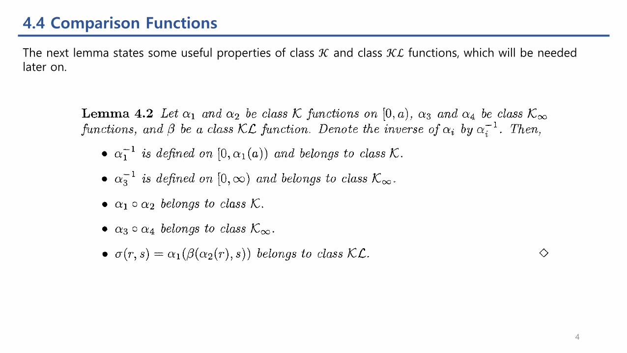
The next lemma states some useful properties of class 𝒦 and class 𝒦ℒ functions, which will be needed later on.
4
4.4 Comparison Functions
5
4.4 Comparison Functions
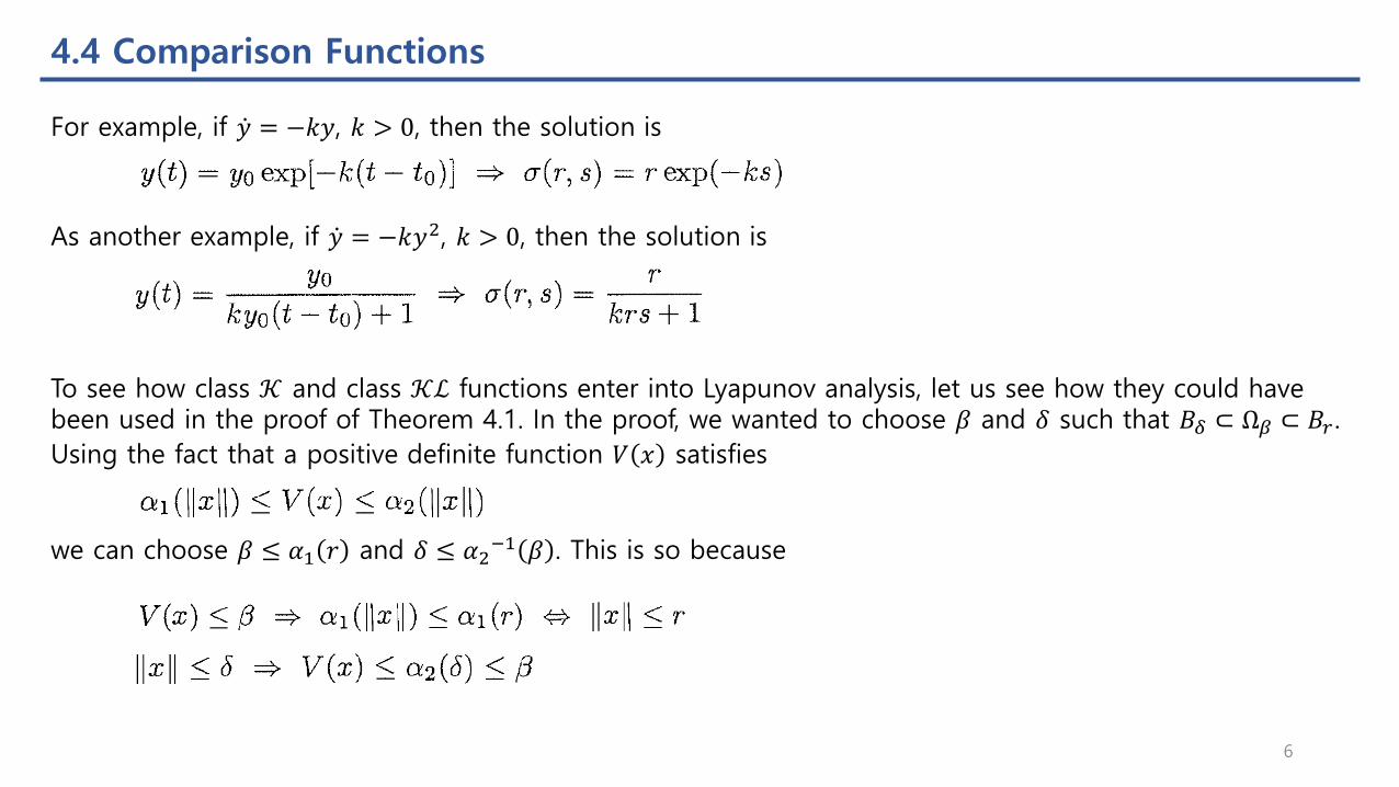
For example, if ሶ𝑦 = −𝑘𝑦, 𝑘 > 0, then the solution is
As another example, if ሶ𝑦 = −𝑘𝑦2, 𝑘 > 0, then the solution is
To see how class 𝒦 and class 𝒦ℒ functions enter into Lyapunov analysis, let us see how they could have been used in the proof of Theorem 4.1. In the proof, we wanted to choose 𝛽 and 𝛿 such that 𝐵𝛿 ⊂ Ω𝛽 ⊂ 𝐵𝑟 .
Using the fact that a positive definite function 𝑉 𝑥 satisfies
we can choose 𝛽 ≤ 𝛼1 𝑟 and 𝛿 ≤ 𝛼2−1 𝛽 . This is so because
6
4.4 Comparison Functions
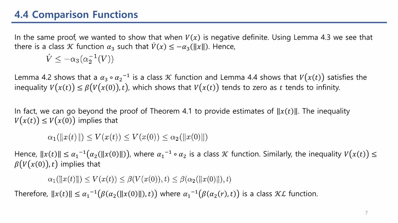
In the same proof, we wanted to show that when 𝑉 𝑥 is negative definite. Using Lemma 4.3 we see that there is a class 𝒦 function 𝛼3 such that ሶ𝑉 𝑥 ≤ −𝛼3 𝑥 . Hence,
Lemma 4.2 shows that a 𝛼3 ∘ 𝛼2−1 is a class 𝒦 function and Lemma 4.4 shows that 𝑉 𝑥 𝑡 satisfies the
inequality 𝑉 𝑥 𝑡 ≤ 𝛽 𝑉 𝑥 0 , 𝑡 , which shows that 𝑉 𝑥 𝑡 tends to zero as 𝑡 tends to infinity.
In fact, we can go beyond the proof of Theorem 4.1 to provide estimates of 𝑥 𝑡 . The inequality
𝑉 𝑥 𝑡 ≤ 𝑉 𝑥 0 implies that
Hence, 𝑥 𝑡 ≤ 𝛼1−1 𝛼2 𝑥 0 , where 𝛼1
−1 ∘ 𝛼2 is a class 𝒦 function. Similarly, the inequality 𝑉 𝑥 𝑡 ≤
𝛽 𝑉 𝑥 0 , 𝑡 implies that
Therefore, 𝑥 𝑡 ≤ 𝛼1−1 𝛽 𝛼2 𝑥 0 , 𝑡 where 𝛼1
−1 𝛽 𝛼2 𝑟 , 𝑡 is a class 𝒦ℒ function.
7

4.5 Nonautonomous Systems
Consider the nonautonomous system
where 𝑓: 0,∞ × 𝐷 → 𝑅𝑛 is piecewise continuous in 𝑡 and locally Lipschitz in 𝑥 on 0,∞ × 𝐷, and 𝐷 ⊂ 𝑅𝑛 is a domain that contains the origin 𝑥 = 0. The origin is an equilibrium point for (4.15) at 𝑡 = 0 if
An equilibrium point at the origin could be a translation of a nonzero equilibrium point or, more generally, a translation of a nonzero solution of the system. Suppose ത𝑦 𝜏 is a solution of the system
defined for all 𝜏 ≥ 𝑎. The change of variables
transforms the system into the form
Since
the origin 𝑥 = 0 is an equilibrium point of the transformed system at 𝑡 = 0.
8
4.5 Nonautonomous Systems
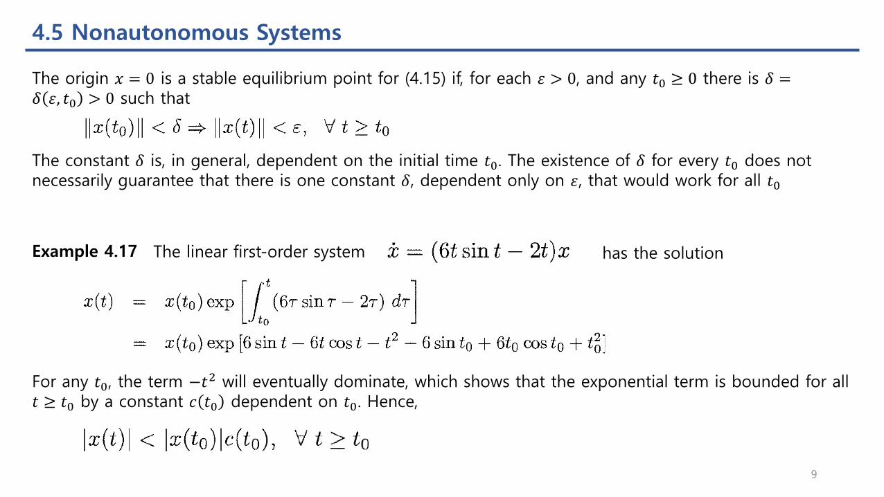
The origin 𝑥 = 0 is a stable equilibrium point for (4.15) if, for each 휀 > 0, and any 𝑡0 ≥ 0 there is 𝛿 =𝛿 휀, 𝑡0 > 0 such that
The constant 𝛿 is, in general, dependent on the initial time 𝑡0. The existence of 𝛿 for every 𝑡0 does not necessarily guarantee that there is one constant 𝛿, dependent only on 휀, that would work for all 𝑡0
Example 4.17 The linear first-order system has the solution
For any 𝑡0, the term −𝑡2 will eventually dominate, which shows that the exponential term is bounded for all 𝑡 ≥ 𝑡0 by a constant 𝑐 𝑡0 dependent on 𝑡0. Hence,
9
4.5 Nonautonomous Systems
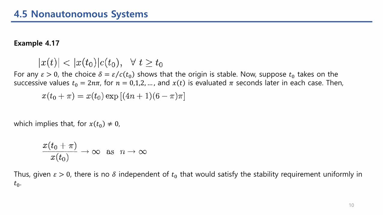
For any 휀 > 0, the choice 𝛿 = Τ휀 𝑐 𝑡0 shows that the origin is stable. Now, suppose 𝑡0 takes on the successive values 𝑡0 = 2𝑛𝜋, for 𝑛 = 0,1,2, … , and 𝑥 𝑡 is evaluated 𝜋 seconds later in each case. Then,
which implies that, for 𝑥 𝑡0 ≠ 0,
Thus, given 휀 > 0, there is no 𝛿 independent of 𝑡0 that would satisfy the stability requirement uniformly in 𝑡0.
Example 4.17
10

4.5 Nonautonomous Systems
Example 4.18 The linear first-order system has the solution
Since 𝑥 𝑡 ≤ 𝑥 𝑡0 , ∀ 𝑡 ≥ 𝑡0, the origin is clearly stable. Actually, given any 휀 > 0, we can choose 𝛿independent of 𝑡0. It is also clear that
Consequently, according to Definition 4.1, the origin is asymptotically stable. Notice, however, that the convergence of 𝑥 𝑡 to the origin is not uniform with respect to the initial time 𝑡0.
Recall that convergence of 𝑥 𝑡 to the origin is equivalent to saying that, given any 휀 > 0, there is 𝑇 =𝑇 휀, 𝑡0 > 0 such that 𝑥 𝑡 < 휀 for all 𝑡 > 𝑡0 + 𝑇. Although this is true for every 𝑡0, the constant 𝑇 cannot be chosen independent of 𝑡0.
11
4.5 Nonautonomous Systems
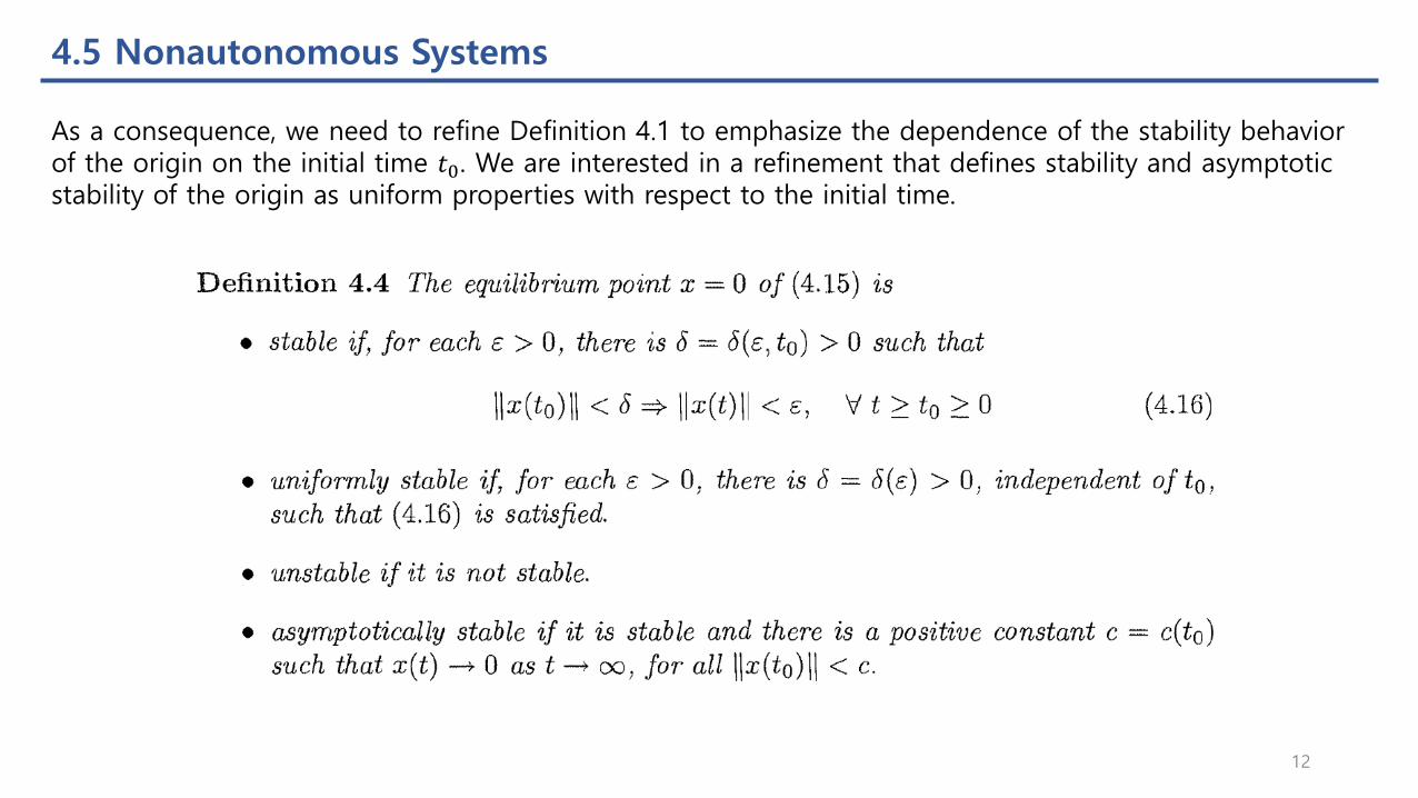
As a consequence, we need to refine Definition 4.1 to emphasize the dependence of the stability behavior of the origin on the initial time 𝑡0. We are interested in a refinement that defines stability and asymptotic stability of the origin as uniform properties with respect to the initial time.
12
4.5 Nonautonomous Systems
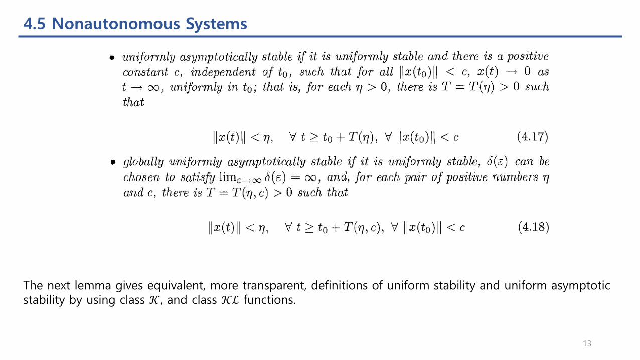
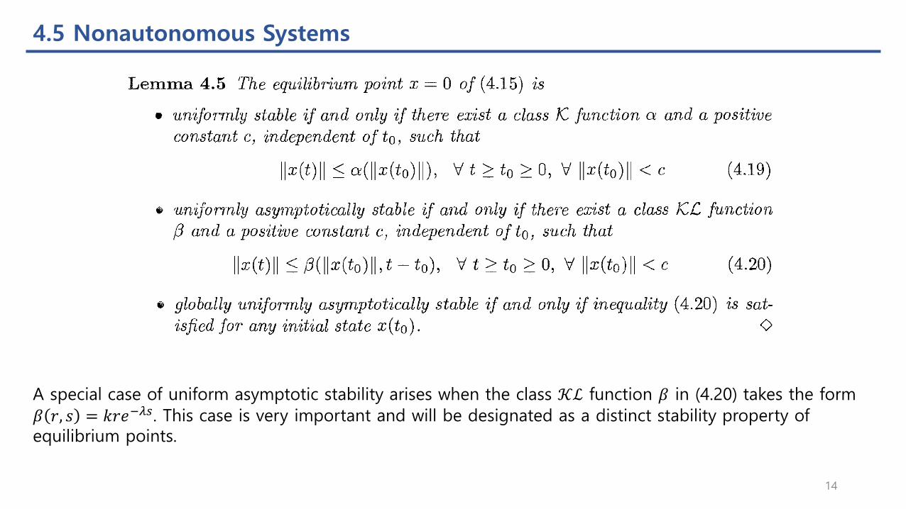
The next lemma gives equivalent, more transparent, definitions of uniform stability and uniform asymptotic stability by using class 𝒦, and class 𝒦ℒ functions.
13
4.5 Nonautonomous Systems
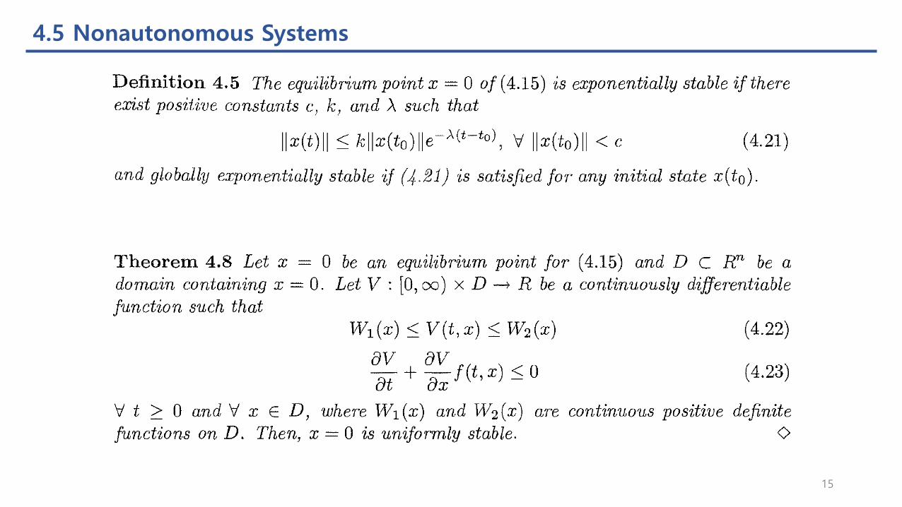
A special case of uniform asymptotic stability arises when the class 𝒦ℒ function 𝛽 in (4.20) takes the form
𝛽 𝑟, 𝑠 = 𝑘𝑟𝑒−𝜆𝑠. This case is very important and will be designated as a distinct stability property of equilibrium points.
14
4.5 Nonautonomous Systems
15
4.5 Nonautonomous Systems
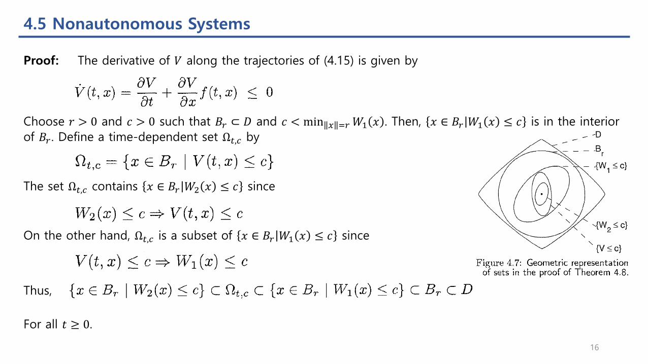
Proof: The derivative of 𝑉 along the trajectories of (4.15) is given by
Choose 𝑟 > 0 and 𝑐 > 0 such that 𝐵𝑟 ⊂ 𝐷 and 𝑐 < min 𝑥 =𝑟𝑊1 𝑥 . Then, 𝑥 ∈ 𝐵𝑟 𝑊1 𝑥 ≤ 𝑐 is in the interior
of 𝐵𝑟 . Define a time-dependent set Ω𝑡,𝑐 by
The set Ω𝑡,𝑐 contains 𝑥 ∈ 𝐵𝑟 𝑊2 𝑥 ≤ 𝑐 since
On the other hand, Ω𝑡,𝑐 is a subset of 𝑥 ∈ 𝐵𝑟 𝑊1 𝑥 ≤ 𝑐 since
Thus,
For all 𝑡 ≥ 0.
16
4.5 Nonautonomous Systems
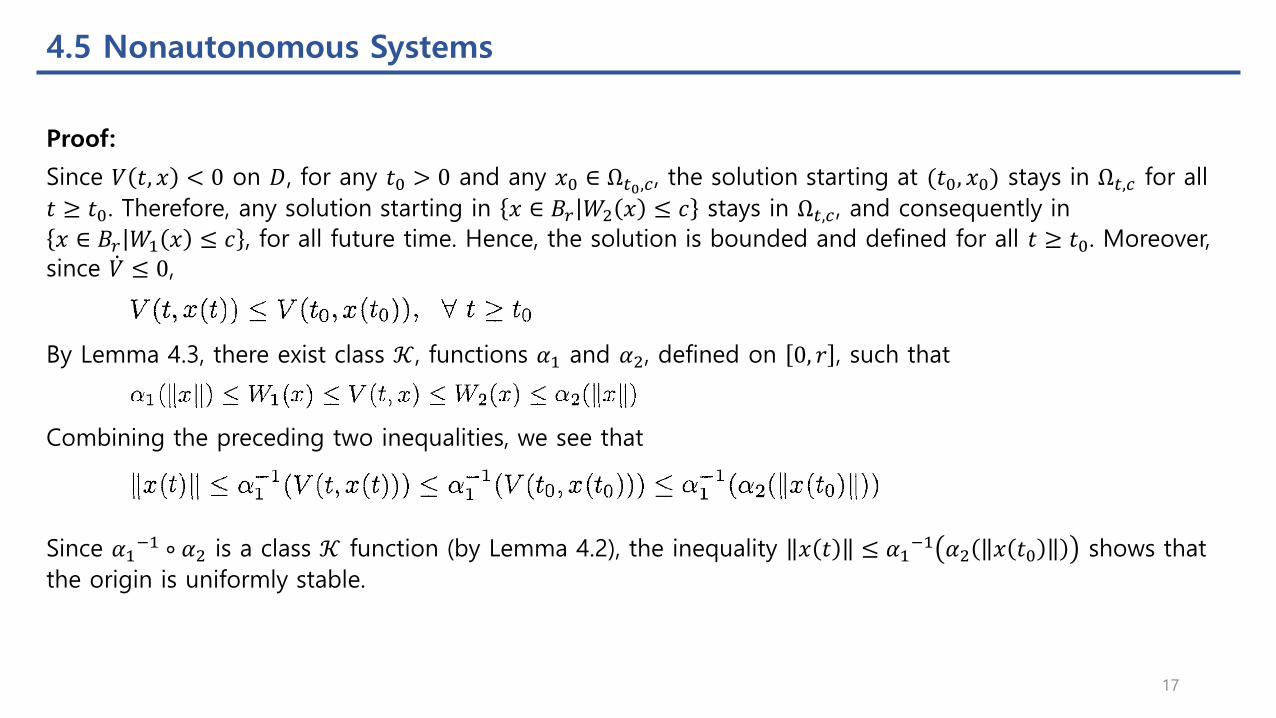
Since 𝑉 𝑡, 𝑥 < 0 on 𝐷, for any 𝑡0 > 0 and any 𝑥0 ∈ Ω𝑡0,𝑐, the solution starting at (𝑡0, 𝑥0) stays in Ω𝑡,𝑐 for all
𝑡 ≥ 𝑡0. Therefore, any solution starting in 𝑥 ∈ 𝐵𝑟 𝑊2 𝑥 ≤ 𝑐 stays in Ω𝑡,𝑐, and consequently in
𝑥 ∈ 𝐵𝑟 𝑊1 𝑥 ≤ 𝑐 , for all future time. Hence, the solution is bounded and defined for all 𝑡 ≥ 𝑡0. Moreover, since ሶ𝑉 ≤ 0,
Proof:
By Lemma 4.3, there exist class 𝒦, functions 𝛼1 and 𝛼2, defined on 0, 𝑟 , such that
Combining the preceding two inequalities, we see that
Since 𝛼1−1 ∘ 𝛼2 is a class 𝒦 function (by Lemma 4.2), the inequality 𝑥 𝑡 ≤ 𝛼1
−1 𝛼2 𝑥 𝑡0 shows that
the origin is uniformly stable.
17
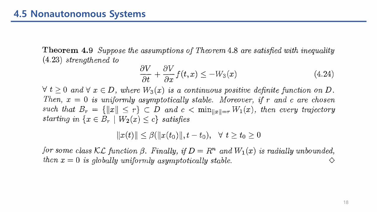
4.5 Nonautonomous Systems
18
4.5 Nonautonomous Systems
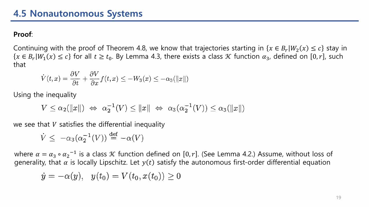
Proof:
Continuing with the proof of Theorem 4.8, we know that trajectories starting in 𝑥 ∈ 𝐵𝑟 𝑊2 𝑥 ≤ 𝑐 stay in 𝑥 ∈ 𝐵𝑟 𝑊1 𝑥 ≤ 𝑐 for all 𝑡 ≥ 𝑡0. By Lemma 4.3, there exists a class 𝒦 function 𝛼3, defined on 0, 𝑟 , such
that
Using the inequality
we see that 𝑉 satisfies the differential inequality
where 𝛼 = 𝛼3 ∘ 𝛼2−1 is a class 𝒦 function defined on 0, 𝑟 . (See Lemma 4.2.) Assume, without loss of
generality, that 𝛼 is locally Lipschitz. Let 𝑦 𝑡 satisfy the autonomous first-order differential equation
19
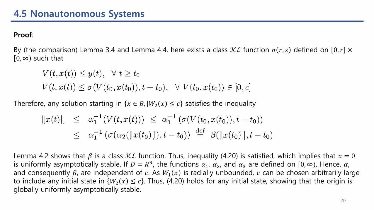
4.5 Nonautonomous Systems
By (the comparison) Lemma 3.4 and Lemma 4.4, here exists a class 𝒦ℒ function 𝜎 𝑟, 𝑠 defined on 0, 𝑟 ×0,∞ such that
Proof:
Therefore, any solution starting in 𝑥 ∈ 𝐵𝑟 𝑊2 𝑥 ≤ 𝑐 satisfies the inequality
Lemma 4.2 shows that 𝛽 is a class 𝒦ℒ function. Thus, inequality (4.20) is satisfied, which implies that 𝑥 = 0is uniformly asymptotically stable. If 𝐷 = 𝑅𝑛, the functions 𝛼1, 𝛼2, and 𝛼3 are defined on [0,∞). Hence, 𝛼, and consequently 𝛽, are independent of 𝑐. As 𝑊1 𝑥 is radially unbounded, 𝑐 can be chosen arbitrarily large to include any initial state in 𝑊2 𝑥 ≤ 𝑐 . Thus, (4.20) holds for any initial state, showing that the origin is globally uniformly asymptotically stable.
20

4.5 Nonautonomous Systems
A function 𝑉 𝑡, 𝑥 is said to be positive semidefinite if 𝑉 𝑡, 𝑥 ≥ 0. It is said to be positive definite if 𝑉 𝑡, 𝑥 ≥𝑊1 𝑥 for some positive definite function 𝑊1 𝑥 , radially unbounded if is so, and decrescent if 𝑉 𝑡, 𝑥 ≤𝑊2 𝑥 .
Therefore, Theorems 4.8 and 4.9 say that the origin is uniformly stable if there is a continuously differentiable, positive definite, decrescent function 𝑉 𝑡, 𝑥 , whose derivative along the trajectories of the system is negative semidefinite. It is uniformly asymptotically stable if the derivative is negative definite, and globally uniformly asymptotically stable if the conditions for uniform, asymptotic stability hold globally with a radially unbounded 𝑉 𝑡, 𝑥 .
21
4.5 Nonautonomous Systems
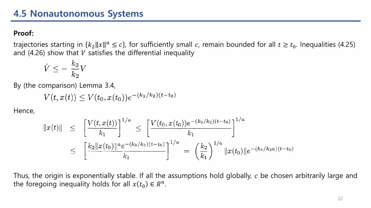
Proof:
trajectories starting in 𝑘2 𝑥 𝑎 ≤ 𝑐 , for sufficiently small 𝑐, remain bounded for all 𝑡 ≥ 𝑡0. Inequalities (4.25) and (4.26) show that 𝑉 satisfies the differential inequality
By (the comparison) Lemma 3.4,
Hence,
Thus, the origin is exponentially stable. If all the assumptions hold globally, 𝑐 be chosen arbitrarily large and the foregoing inequality holds for all 𝑥 𝑡0 ∈ 𝑅𝑛.
22
4.5 Nonautonomous Systems
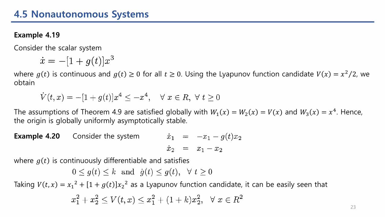
Example 4.19
Consider the scalar system
where 𝑔 𝑡 is continuous and 𝑔 𝑡 ≥ 0 for all 𝑡 ≥ 0. Using the Lyapunov function candidate 𝑉 𝑥 = Τ𝑥2 2, we obtain
The assumptions of Theorem 4.9 are satisfied globally with 𝑊1 𝑥 = 𝑊2 𝑥 = 𝑉(𝑥) and 𝑊3 𝑥 = 𝑥4. Hence, the origin is globally uniformly asymptotically stable.
Example 4.20 Consider the system
where 𝑔 𝑡 is continuously differentiable and satisfies
Taking 𝑉 𝑡, 𝑥 = 𝑥12 + 1 + 𝑔 𝑡 𝑥2
2 as a Lyapunov function candidate, it can be easily seen that
23
4.5 Nonautonomous Systems
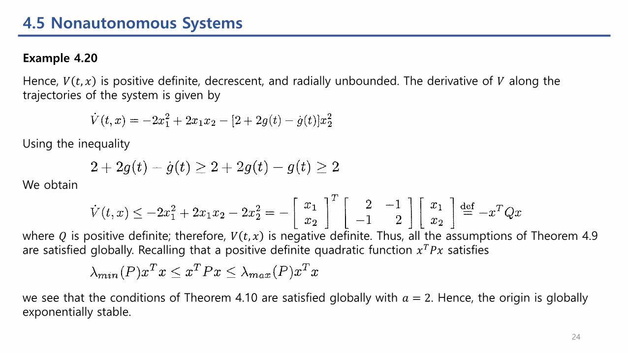
Example 4.20
Hence, 𝑉 𝑡, 𝑥 is positive definite, decrescent, and radially unbounded. The derivative of 𝑉 along the trajectories of the system is given by
Using the inequality
We obtain
where 𝑄 is positive definite; therefore, 𝑉 𝑡, 𝑥 is negative definite. Thus, all the assumptions of Theorem 4.9 are satisfied globally. Recalling that a positive definite quadratic function 𝑥𝑇𝑃𝑥 satisfies
we see that the conditions of Theorem 4.10 are satisfied globally with 𝑎 = 2. Hence, the origin is globally exponentially stable.
24

4.5 Nonautonomous Systems
Example 4.21 The linear time-varying system
has an equilibrium point at 𝑥 = 0. Let 𝐴 𝑡 be continuous for all 𝑡 ≥ 0. Suppose there is a continuously differentiable, symmetric, bounded, positive definite matrix 𝑃 𝑡 ; that is,
which satisfies the matrix differential equation
where 𝑄 𝑡 is continuous, symmetric, and positive definite; that is,
The Lyapunov function candidate
satisfies
and its derivative along the trajectories of the system (4.27) is given by
Thus, all the assumptions of Theorem 4.10 are satisfied globally with 𝑎 = 2, and we conclude that the origin is globally exponentially stable.
25
4.6 Linear Time-Varying Systems and Linearization
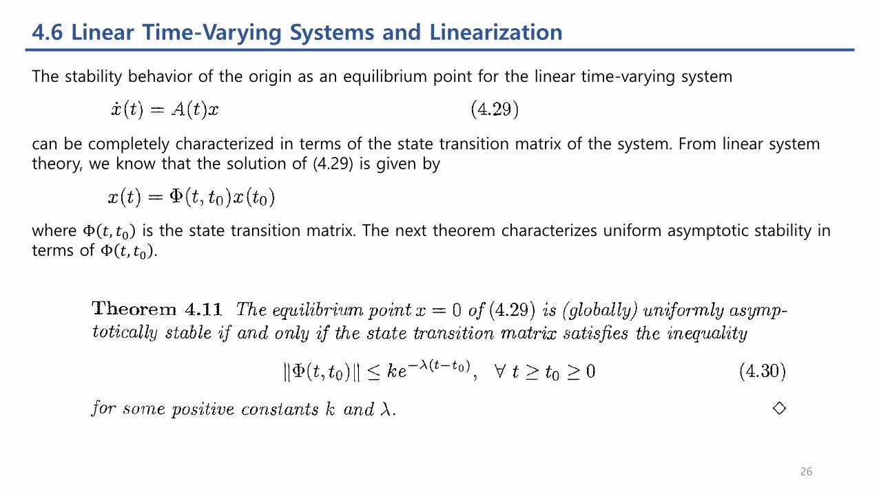
The stability behavior of the origin as an equilibrium point for the linear time-varying system
can be completely characterized in terms of the state transition matrix of the system. From linear system theory, we know that the solution of (4.29) is given by
where Φ 𝑡, 𝑡0 is the state transition matrix. The next theorem characterizes uniform asymptotic stability in terms of Φ 𝑡, 𝑡0 .
26
4.6 Linear Time-Varying Systems and Linearization
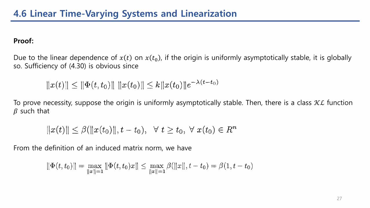
Proof:
Due to the linear dependence of 𝑥 𝑡 on 𝑥 𝑡0 , if the origin is uniformly asymptotically stable, it is globally so. Sufficiency of (4.30) is obvious since
To prove necessity, suppose the origin is uniformly asymptotically stable. Then, there is a class 𝒦ℒ function 𝛽 such that
From the definition of an induced matrix norm, we have
27
4.6 Linear Time-Varying Systems and Linearization
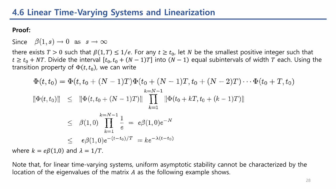
Since
Proof:
there exists 𝑇 > 0 such that 𝛽 1, 𝑇 ≤ Τ1 𝑒. For any 𝑡 ≥ 𝑡0, let 𝑁 be the smallest positive integer such that 𝑡 ≥ 𝑡0 + 𝑁𝑇. Divide the interval 𝑡0, 𝑡0 + 𝑁 − 1 𝑇 into 𝑁 − 1 equal subintervals of width 𝑇 each. Using the transition property of Φ 𝑡, 𝑡0 , we can write
where 𝑘 = 𝑒𝛽 1,0 and 𝜆 = Τ1 𝑇.
Note that, for linear time-varying systems, uniform asymptotic stability cannot be characterized by the location of the eigenvalues of the matrix 𝐴 as the following example shows.
28
4.6 Linear Time-Varying Systems and Linearization
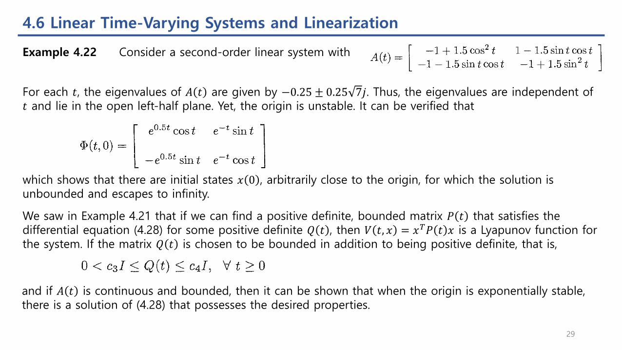
Example 4.22 Consider a second-order linear system with
For each 𝑡, the eigenvalues of 𝐴 𝑡 are given by −0.25 ± 0.25 7𝑗. Thus, the eigenvalues are independent of 𝑡 and lie in the open left-half plane. Yet, the origin is unstable. It can be verified that
which shows that there are initial states 𝑥 0 , arbitrarily close to the origin, for which the solution is unbounded and escapes to infinity.
We saw in Example 4.21 that if we can find a positive definite, bounded matrix 𝑃 𝑡 that satisfies the differential equation (4.28) for some positive definite 𝑄 𝑡 , then 𝑉 𝑡, 𝑥 = 𝑥𝑇𝑃 𝑡 𝑥 is a Lyapunov function for the system. If the matrix 𝑄 𝑡 is chosen to be bounded in addition to being positive definite, that is,
and if 𝐴 𝑡 is continuous and bounded, then it can be shown that when the origin is exponentially stable, there is a solution of (4.28) that possesses the desired properties.
29
4.6 Linear Time-Varying Systems and Linearization
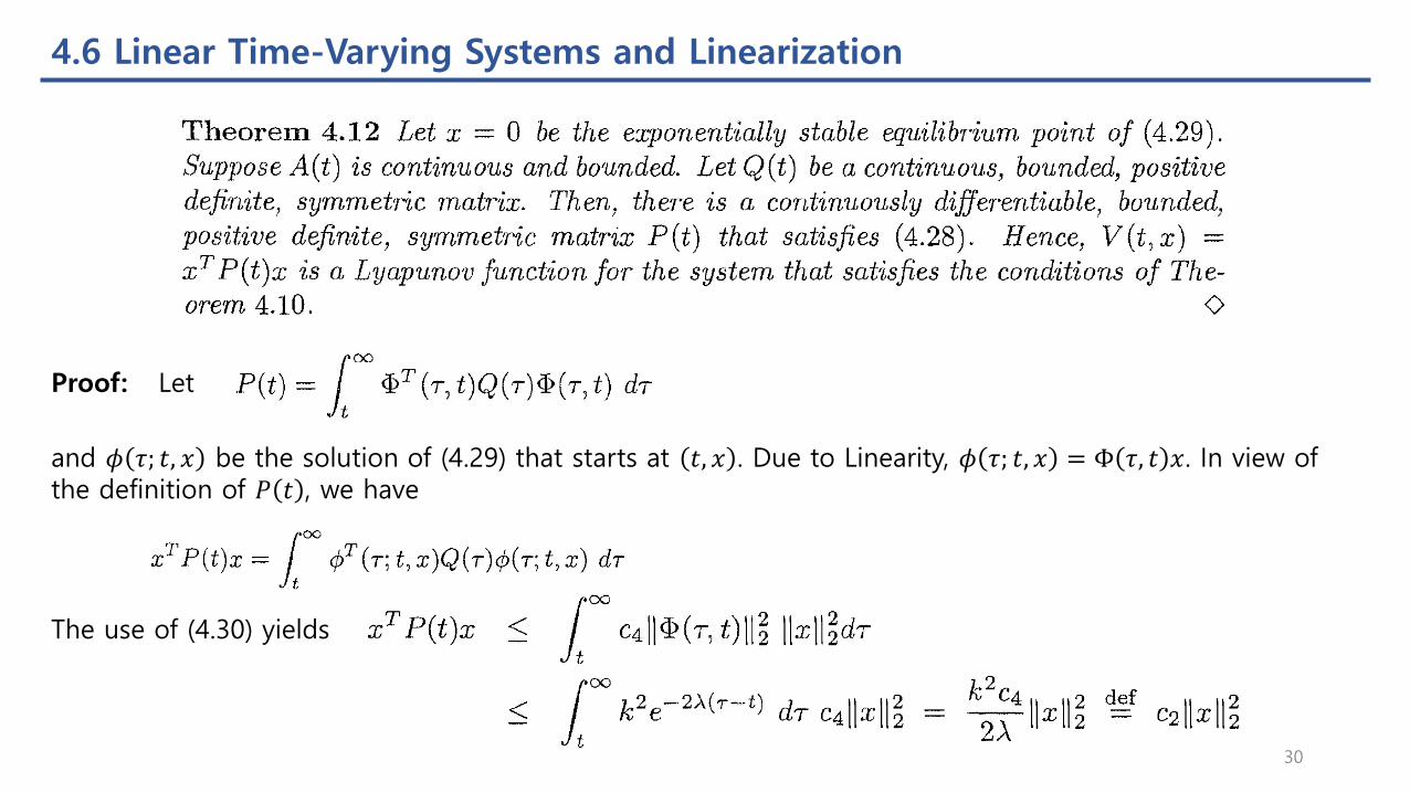
Proof: Let
and 𝜙 𝜏; 𝑡, 𝑥 be the solution of (4.29) that starts at 𝑡, 𝑥 . Due to Linearity, 𝜙 𝜏; 𝑡, 𝑥 = Φ 𝜏, 𝑡 𝑥. In view of the definition of 𝑃 𝑡 , we have
The use of (4.30) yields
30

4.6 Linear Time-Varying Systems and Linearization
Proof: On the other hand, since
the solution 𝜙 𝜏; 𝑡, 𝑥 satisfies the lower bound
Hence,
Thus,
which shows that 𝑃 𝑡 is positive definite and bounded. The definition of 𝑃 𝑡 shows that it is symmetric and continuously differentiable. The fact that 𝑃 𝑡 satisfies (4.28) can be shown by differentiating 𝑃 𝑡 and using the property
31
4.6 Linear Time-Varying Systems and Linearization
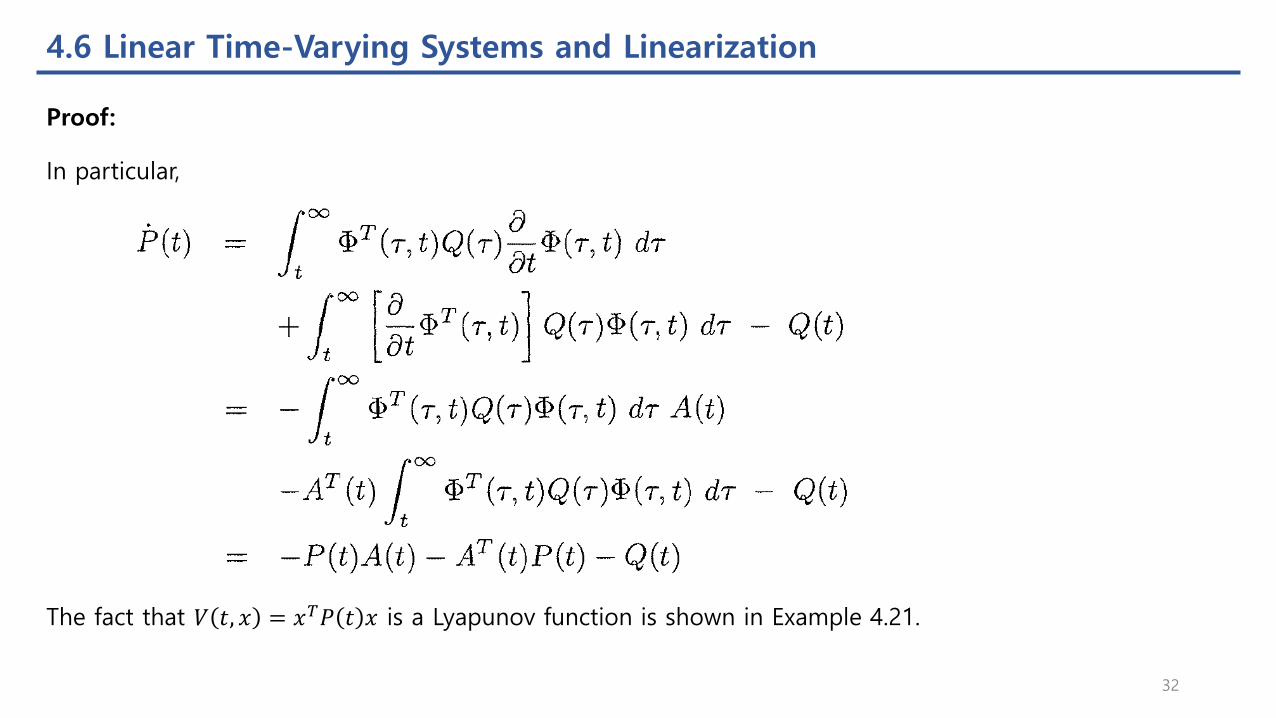
In particular,
The fact that 𝑉 𝑡, 𝑥 = 𝑥𝑇𝑃 𝑡 𝑥 is a Lyapunov function is shown in Example 4.21.
Proof:
32

4.6 Linear Time-Varying Systems and Linearization
Consider the nonlinear nonautonomous system
where 𝑓: 0,∞ × 𝐷 → 𝑅𝑛 is continuously differentiable and 𝐷 = 𝑥 ∈ 𝑅𝑛 𝑥 2 < 𝑟 . Suppose the origin 𝑥 = 0is an equilibrium point for the system at 𝑡 = 0; that is, 𝑓 𝑡, 0 = 0 for all 𝑡 ≥ 0. Furthermore, suppose the Jacobian matrix Τ𝑑𝑓 𝑑𝑥 is bounded and Lipschitz on 𝐷, uniformly in 𝑡; thus,
for all 1 < 𝑖 < 𝑛. By the mean value theorem,
where 𝑧𝑖 is a point on the line segment connecting 𝑥 to the origin. Since 𝑓 𝑡, 0 = 0, we can write 𝑓𝑖 𝑡, 𝑥 as
33
4.6 Linear Time-Varying Systems and Linearization
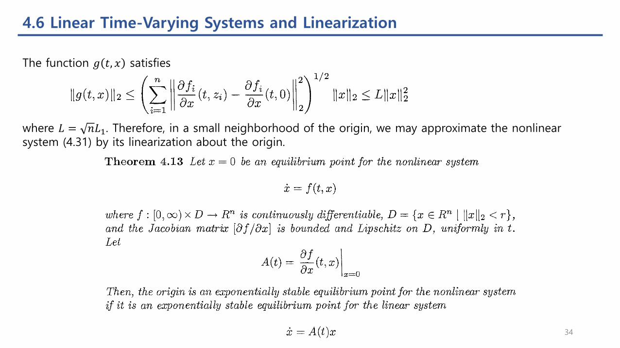
The function 𝑔 𝑡, 𝑥 satisfies
where 𝐿 = 𝑛𝐿1. Therefore, in a small neighborhood of the origin, we may approximate the nonlinear system (4.31) by its linearization about the origin.
34
4.6 Linear Time-Varying Systems and Linearization
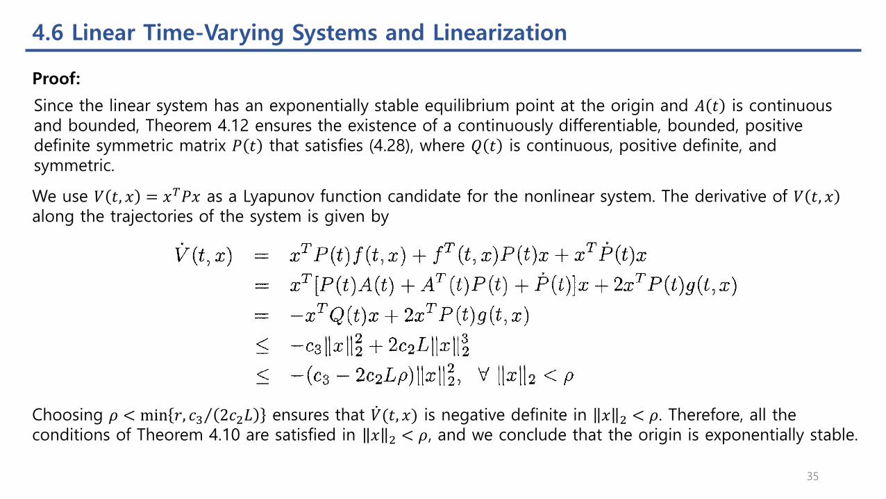
Proof:
Since the linear system has an exponentially stable equilibrium point at the origin and 𝐴 𝑡 is continuous and bounded, Theorem 4.12 ensures the existence of a continuously differentiable, bounded, positive definite symmetric matrix 𝑃 𝑡 that satisfies (4.28), where 𝑄 𝑡 is continuous, positive definite, and symmetric.
We use 𝑉 𝑡, 𝑥 = 𝑥𝑇𝑃𝑥 as a Lyapunov function candidate for the nonlinear system. The derivative of 𝑉 𝑡, 𝑥along the trajectories of the system is given by
Choosing 𝜌 < min 𝑟, Τ𝑐3 2𝑐2𝐿 ensures that ሶ𝑉(𝑡, 𝑥) is negative definite in 𝑥 2 < 𝜌. Therefore, all the conditions of Theorem 4.10 are satisfied in 𝑥 2 < 𝜌, and we conclude that the origin is exponentially stable.
35
4.7 Converse Theorems
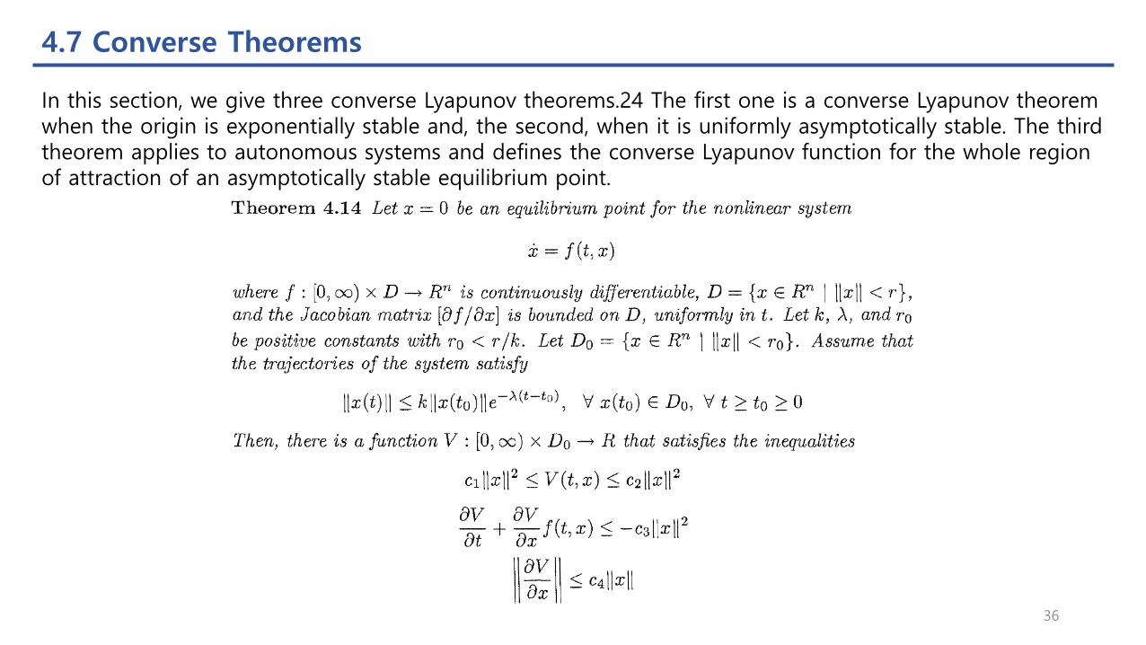
In this section, we give three converse Lyapunov theorems.24 The first one is a converse Lyapunov theorem when the origin is exponentially stable and, the second, when it is uniformly asymptotically stable. The third theorem applies to autonomous systems and defines the converse Lyapunov function for the whole region of attraction of an asymptotically stable equilibrium point.
36
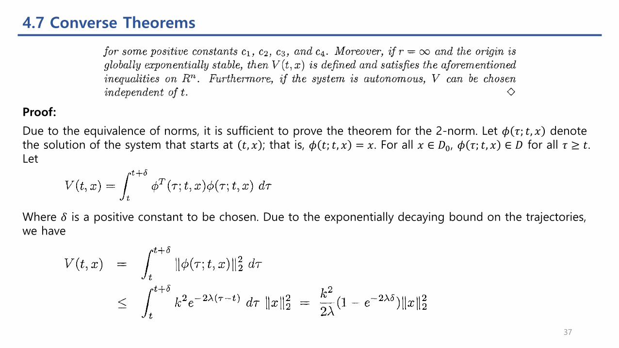
4.7 Converse Theorems
Proof:
Due to the equivalence of norms, it is sufficient to prove the theorem for the 2-norm. Let 𝜙 𝜏; 𝑡, 𝑥 denote the solution of the system that starts at 𝑡, 𝑥 ; that is, 𝜙 𝑡; 𝑡, 𝑥 = 𝑥. For all 𝑥 ∈ 𝐷0, 𝜙 𝜏; 𝑡, 𝑥 ∈ 𝐷 for all 𝜏 ≥ 𝑡. Let
Where 𝛿 is a positive constant to be chosen. Due to the exponentially decaying bound on the trajectories, we have
37

4.7 Converse Theorems
On the other hand, the Jacobian matrix 𝑑𝑓/𝑑𝑥 is bounded on 𝐷. Let
Proof:
Then, 𝑓 𝑡, 𝑥 2 ≤ 𝐿 𝑥 2 and 𝜙 𝜏; 𝑡, 𝑥 satisfies the lower bound
Hence,
Thus, 𝑉 𝑡, 𝑥 satisfies the first inequality of the theorem with
38
4.7 Converse Theorems
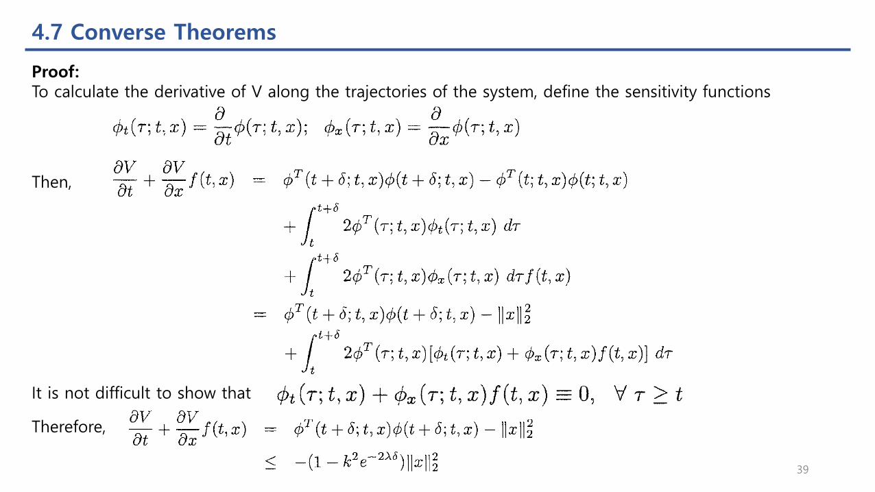
To calculate the derivative of V along the trajectories of the system, define the sensitivity functions
Then,
It is not difficult to show that
Proof:
Therefore,
39
4.7 Converse Theorems
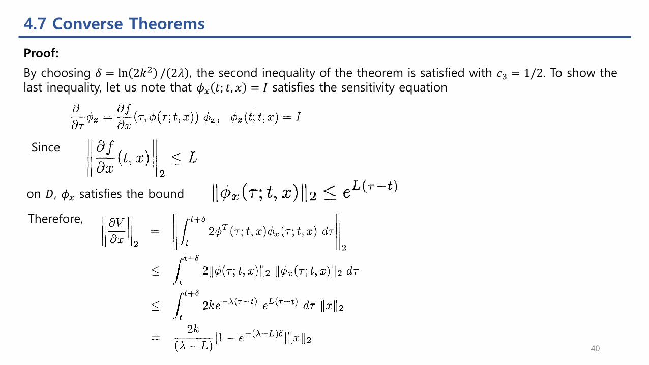
Since
on 𝐷, 𝜙𝑥 satisfies the bound
Therefore,
By choosing 𝛿 = ln 2𝑘2 / 2𝜆 , the second inequality of the theorem is satisfied with 𝑐3 = 1/2. To show the last inequality, let us note that 𝜙𝑥 𝑡; 𝑡, 𝑥 = 𝐼 satisfies the sensitivity equation
Proof:
40
4.7 Converse Theorems
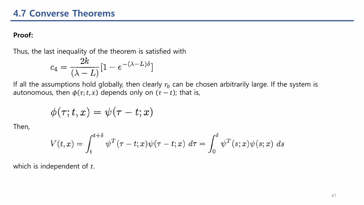
Thus, the last inequality of the theorem is satisfied with
If all the assumptions hold globally, then clearly 𝑟0 can be chosen arbitrarily large. If the system is autonomous, then 𝜙 𝜏; 𝑡, 𝑥 depends only on 𝜏 − 𝑡 ; that is,
Then,
which is independent of 𝑡.
Proof:
41
4.7 Converse Theorems
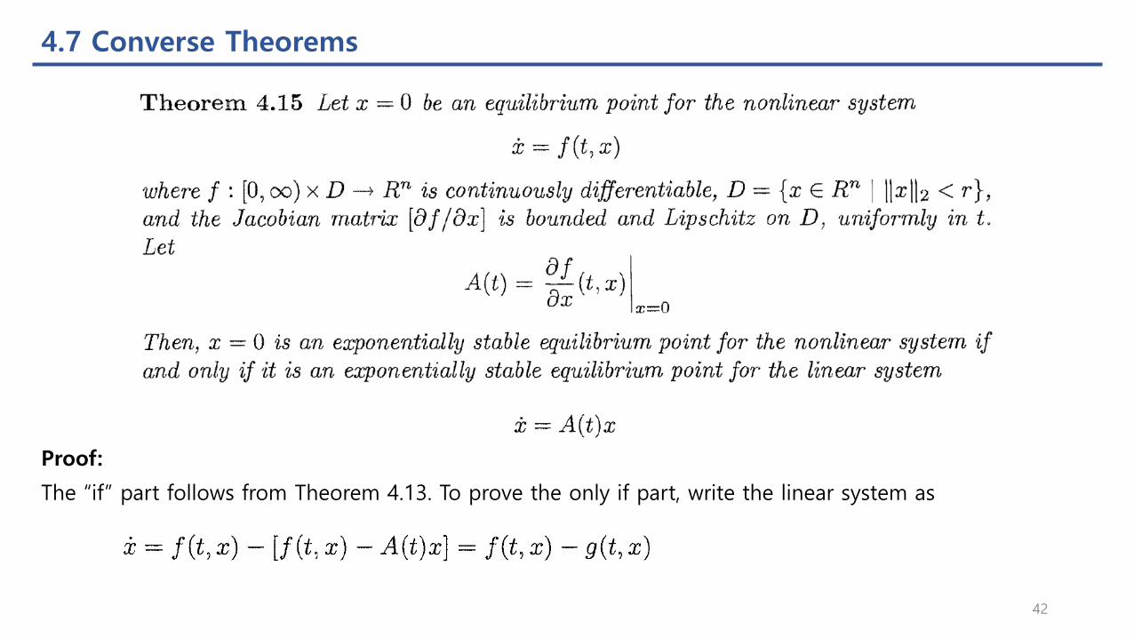
Proof:
The “if” part follows from Theorem 4.13. To prove the only if part, write the linear system as
42
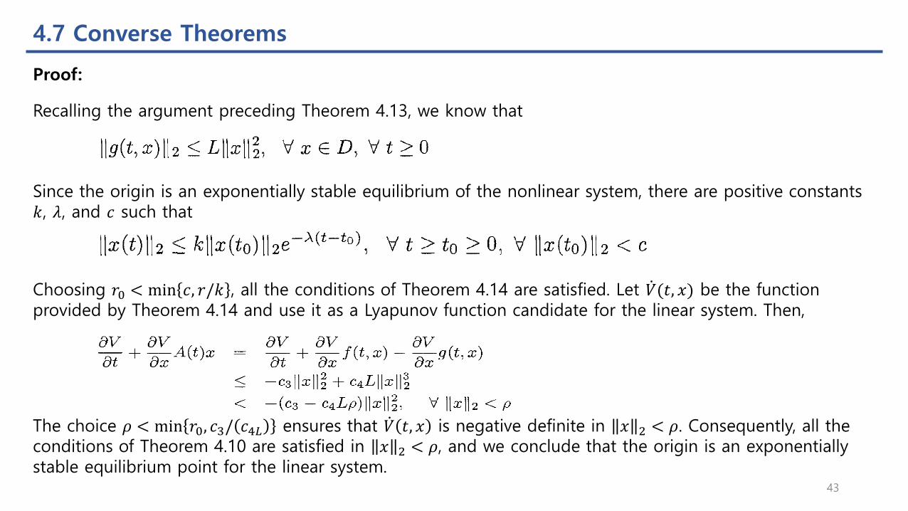
The choice 𝜌 < min 𝑟0, 𝑐3/ 𝑐4𝐿 ensures that ሶ𝑉 𝑡, 𝑥 is negative definite in 𝑥 2 < 𝜌. Consequently, all the conditions of Theorem 4.10 are satisfied in 𝑥 2 < 𝜌, and we conclude that the origin is an exponentially stable equilibrium point for the linear system.
4.7 Converse Theorems
Proof:
Recalling the argument preceding Theorem 4.13, we know that
Since the origin is an exponentially stable equilibrium of the nonlinear system, there are positive constants 𝑘, 𝜆, and 𝑐 such that
Choosing 𝑟0 < min 𝑐, 𝑟/𝑘 , all the conditions of Theorem 4.14 are satisfied. Let ሶ𝑉(𝑡, 𝑥) be the function provided by Theorem 4.14 and use it as a Lyapunov function candidate for the linear system. Then,
43
4.7 Converse Theorems
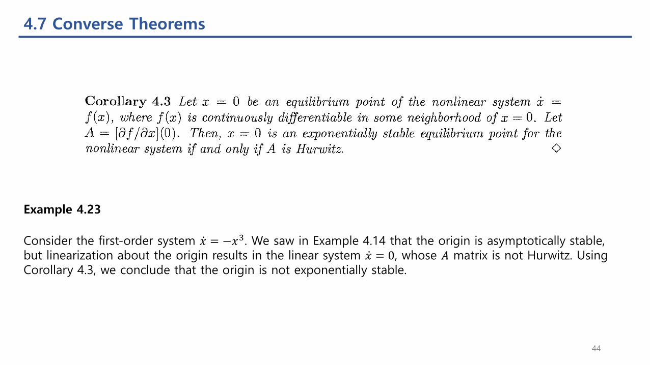
Example 4.23
Consider the first-order system ሶ𝑥 = −𝑥3. We saw in Example 4.14 that the origin is asymptotically stable, but linearization about the origin results in the linear system ሶ𝑥 = 0, whose 𝐴 matrix is not Hurwitz. Using Corollary 4.3, we conclude that the origin is not exponentially stable.
44
4.7 Converse Theorems
45
4.7 Converse Theorems
46
4.8 Boundedness and Ultimate Boundedness
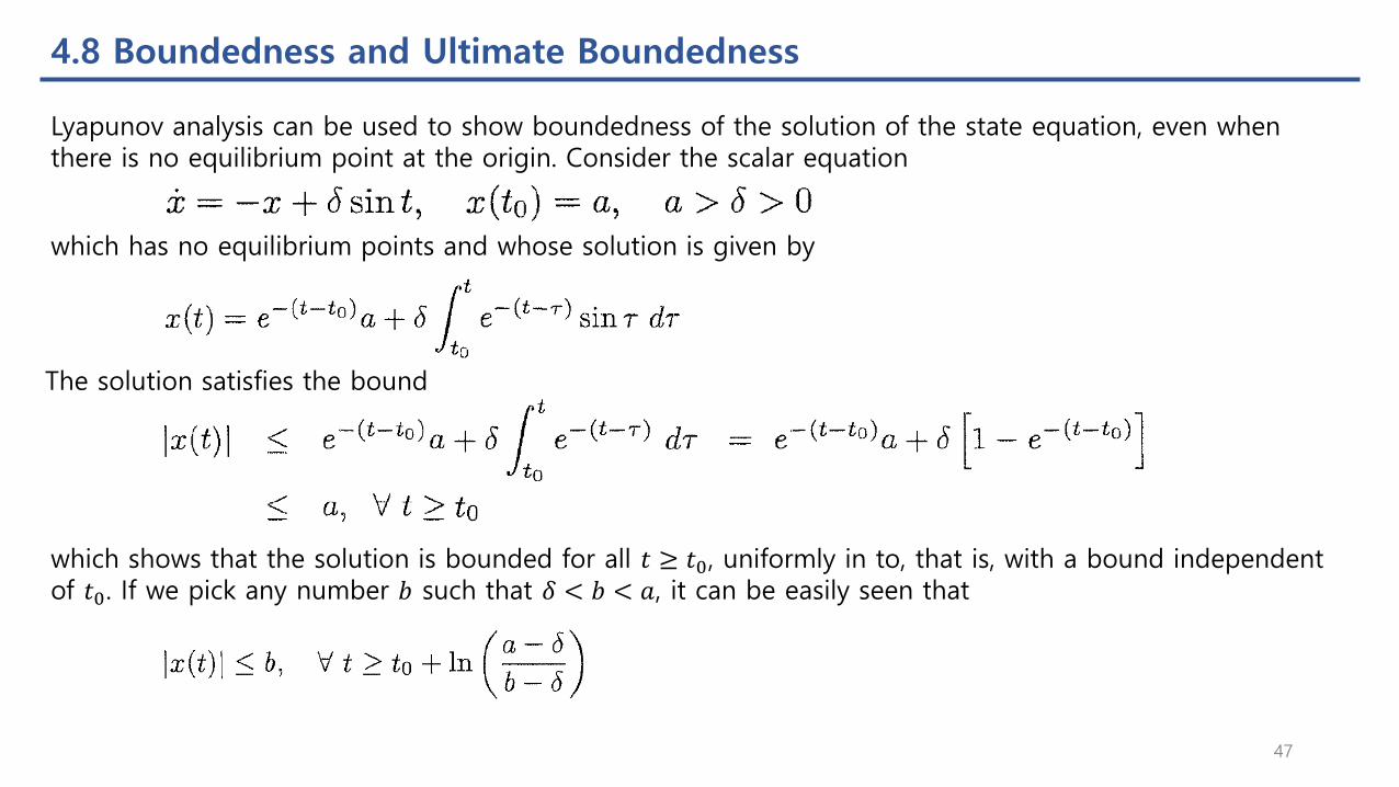
Lyapunov analysis can be used to show boundedness of the solution of the state equation, even when there is no equilibrium point at the origin. Consider the scalar equation
which has no equilibrium points and whose solution is given by
The solution satisfies the bound
which shows that the solution is bounded for all 𝑡 ≥ 𝑡0, uniformly in to, that is, with a bound independent of 𝑡0. If we pick any number 𝑏 such that 𝛿 < 𝑏 < 𝑎, it can be easily seen that
47
4.8 Boundedness and Ultimate Boundedness
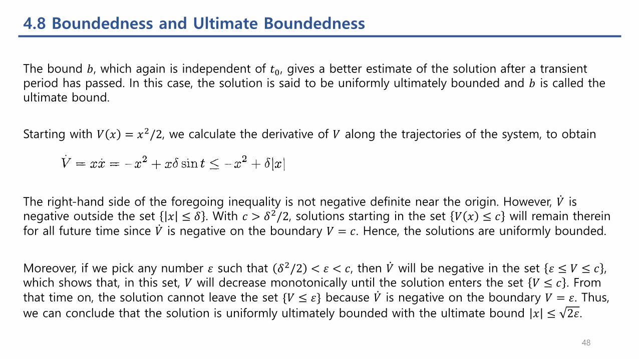
The bound 𝑏, which again is independent of 𝑡0, gives a better estimate of the solution after a transient period has passed. In this case, the solution is said to be uniformly ultimately bounded and 𝑏 is called the ultimate bound.
Starting with 𝑉 𝑥 = 𝑥2/2, we calculate the derivative of 𝑉 along the trajectories of the system, to obtain
The right-hand side of the foregoing inequality is not negative definite near the origin. However, ሶ𝑉 is negative outside the set 𝑥 ≤ 𝛿 . With 𝑐 > 𝛿2/2, solutions starting in the set 𝑉 𝑥 ≤ 𝑐 will remain therein for all future time since ሶ𝑉 is negative on the boundary 𝑉 = 𝑐. Hence, the solutions are uniformly bounded.
Moreover, if we pick any number 휀 such that 𝛿2/2 < 휀 < 𝑐, then ሶ𝑉 will be negative in the set 휀 ≤ 𝑉 ≤ 𝑐 , which shows that, in this set, 𝑉 will decrease monotonically until the solution enters the set 𝑉 ≤ 𝑐 . From that time on, the solution cannot leave the set {𝑉 ≤ 휀} because ሶ𝑉 is negative on the boundary 𝑉 = 휀. Thus,
we can conclude that the solution is uniformly ultimately bounded with the ultimate bound 𝑥 ≤ 2휀.
48
4.8 Boundedness and Ultimate Boundedness
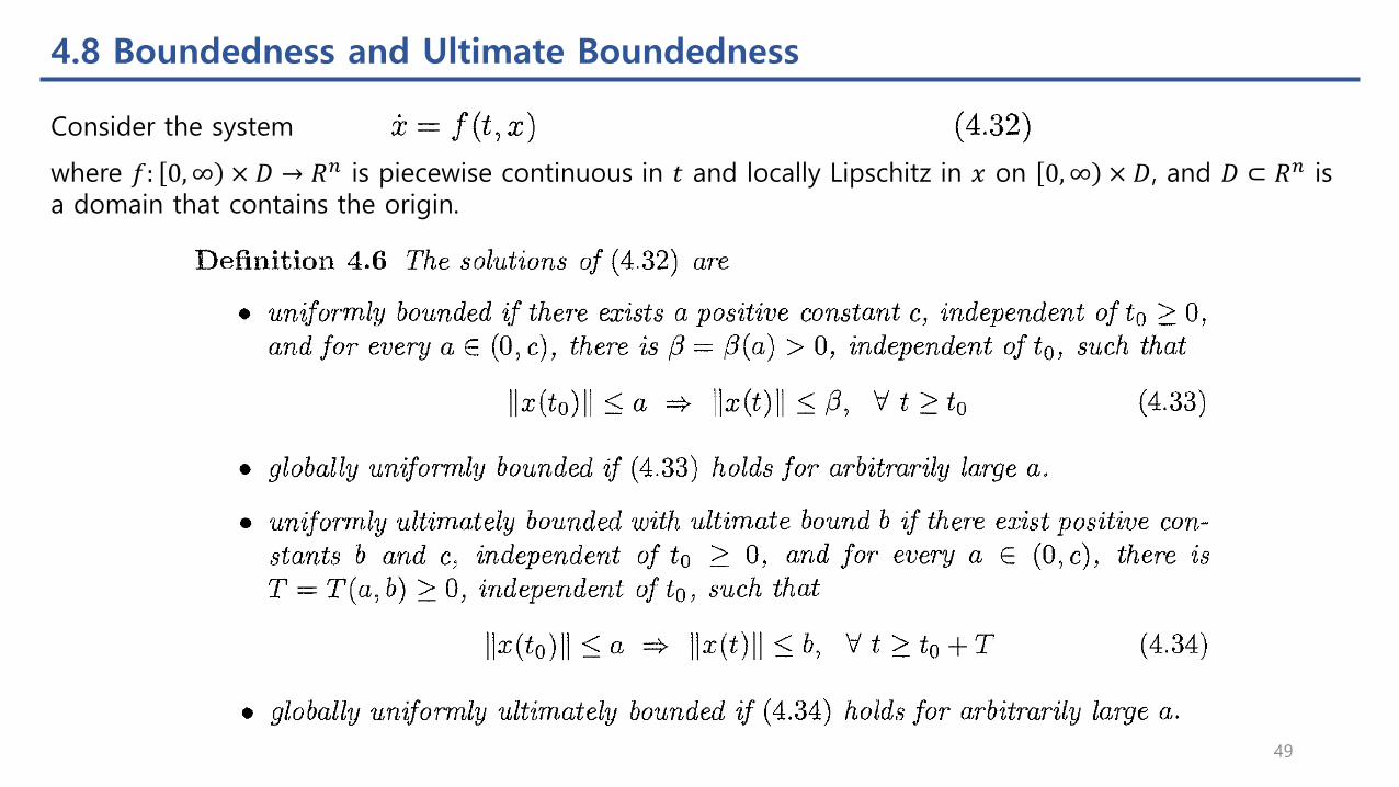
Consider the system
where 𝑓: 0,∞ × 𝐷 → 𝑅𝑛 is piecewise continuous in 𝑡 and locally Lipschitz in 𝑥 on 0,∞ × 𝐷, and 𝐷 ⊂ 𝑅𝑛 is a domain that contains the origin.
49
4.8 Boundedness and Ultimate Boundedness
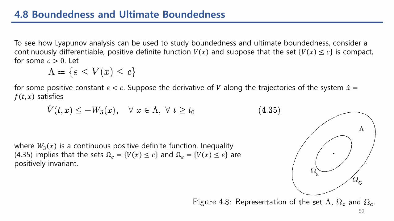
To see how Lyapunov analysis can be used to study boundedness and ultimate boundedness, consider a continuously differentiable, positive definite function 𝑉 𝑥 and suppose that the set 𝑉 𝑥 ≤ 𝑐 is compact, for some 𝑐 > 0. Let
for some positive constant 휀 < 𝑐. Suppose the derivative of 𝑉 along the trajectories of the system ሶ𝑥 =𝑓 𝑡, 𝑥 satisfies
where 𝑊3 𝑥 is a continuous positive definite function. Inequality (4.35) implies that the sets Ω𝑐 = 𝑉 𝑥 ≤ 𝑐 and Ω = 𝑉 𝑥 ≤ 휀 are positively invariant.
50
4.8 Boundedness and Ultimate Boundedness
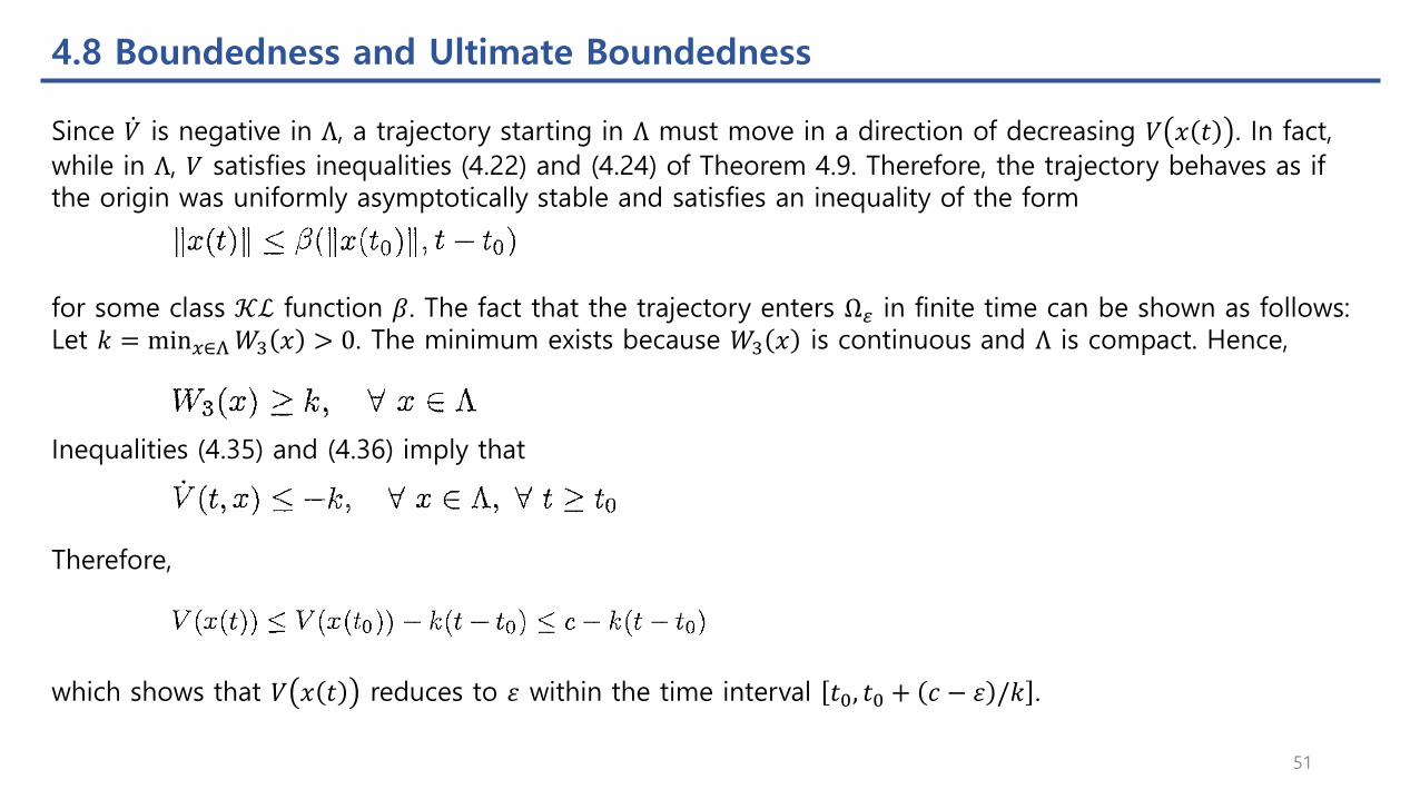
Since ሶ𝑉 is negative in Λ, a trajectory starting in Λ must move in a direction of decreasing 𝑉 𝑥 𝑡 . In fact,
while in Λ, 𝑉 satisfies inequalities (4.22) and (4.24) of Theorem 4.9. Therefore, the trajectory behaves as if the origin was uniformly asymptotically stable and satisfies an inequality of the form
for some class 𝒦ℒ function 𝛽. The fact that the trajectory enters Ω in finite time can be shown as follows: Let 𝑘 = min𝑥∈Λ𝑊3 𝑥 > 0. The minimum exists because 𝑊3 𝑥 is continuous and Λ is compact. Hence,
Inequalities (4.35) and (4.36) imply that
Therefore,
which shows that 𝑉 𝑥 𝑡 reduces to 휀 within the time interval 𝑡0, 𝑡0 + 𝑐 − 휀 /𝑘 .
51
4.8 Boundedness and Ultimate Boundedness
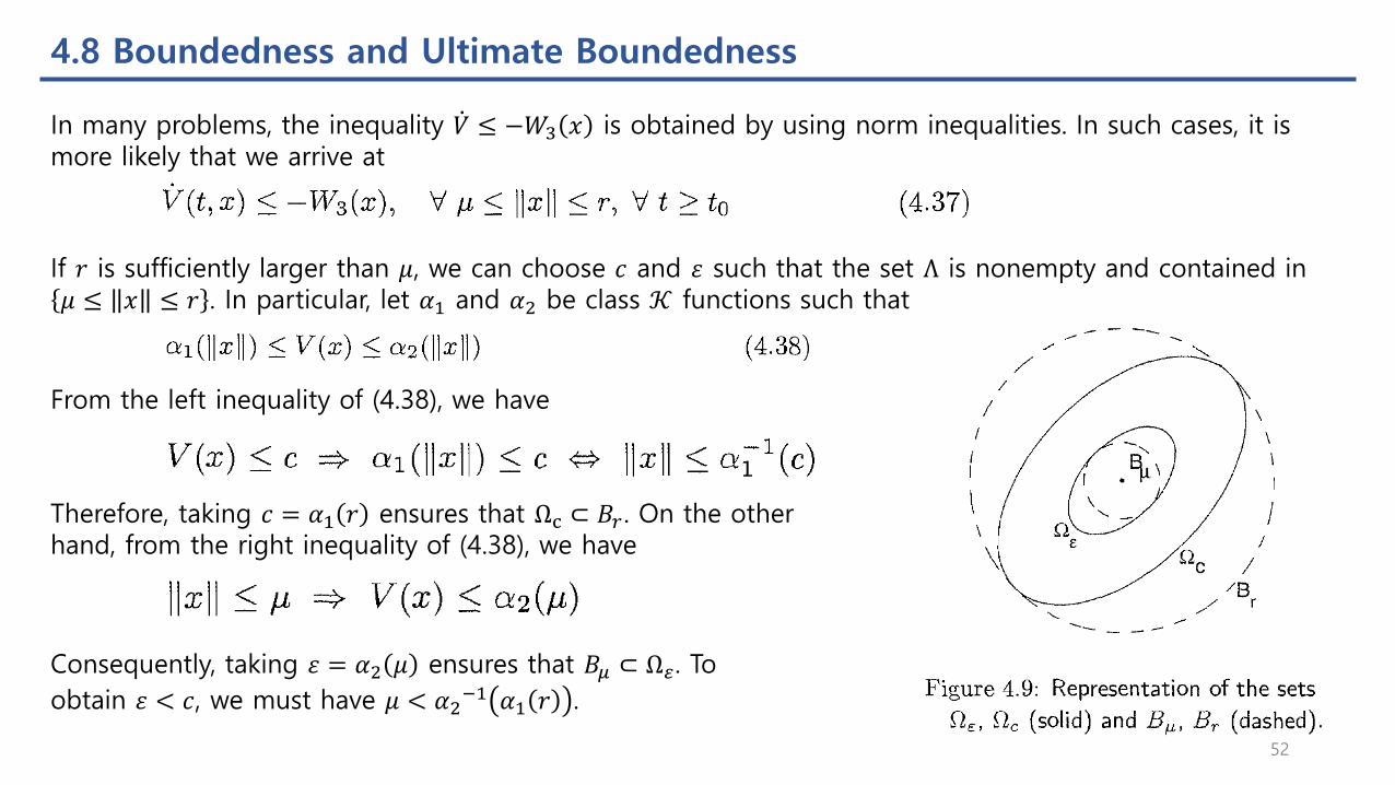
In many problems, the inequality ሶ𝑉 ≤ −𝑊3 𝑥 is obtained by using norm inequalities. In such cases, it is more likely that we arrive at
If 𝑟 is sufficiently larger than 𝜇, we can choose 𝑐 and 휀 such that the set Λ is nonempty and contained in 𝜇 ≤ 𝑥 ≤ 𝑟 . In particular, let 𝛼1 and 𝛼2 be class 𝒦 functions such that
From the left inequality of (4.38), we have
Therefore, taking 𝑐 = 𝛼1 𝑟 ensures that Ωc ⊂ 𝐵𝑟 . On the other hand, from the right inequality of (4.38), we have
Consequently, taking 휀 = 𝛼2 𝜇 ensures that 𝐵𝜇 ⊂ Ω . To
obtain 휀 < 𝑐, we must have 𝜇 < 𝛼2−1 𝛼1 𝑟 .
52

4.8 Boundedness and Ultimate Boundedness
The foregoing argument shows that all trajectories starting in Ω𝑐 enter Ω within a finite time 𝑇. To calculate the ultimate bound on 𝑥 𝑡 , we use the left inequality of (4.38) to write
Recalling that 휀 = 𝛼2 𝜇 , we see that
Therefore, the ultimate bound can be taken as 𝑏 = 𝛼1−1 𝛼2 𝜇 .
53

4.8 Boundedness and Ultimate Boundedness
Inequalities (4.42) and (4.43) show that 𝑥 𝑡 is uniformly bounded for all 𝑡 ≥ 𝑡0 and uniformly ultimately
bounded with the ultimate bound 𝛼1−1 𝛼2 𝜇 . The ultimate bound is a class 𝒦 function of 𝜇; hence, the
smaller the value of 𝜇, the smaller the ultimate bound. As 𝜇 → 0, the ultimate bound approaches zero.
54
4.8 Boundedness and Ultimate Boundedness
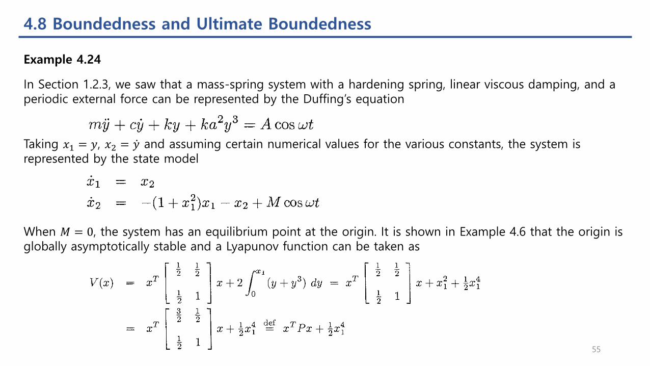
Example 4.24
In Section 1.2.3, we saw that a mass-spring system with a hardening spring, linear viscous damping, and a periodic external force can be represented by the Duffing’s equation
Taking 𝑥1 = 𝑦, 𝑥2 = ሶ𝑦 and assuming certain numerical values for the various constants, the system is represented by the state model
When 𝑀 = 0, the system has an equilibrium point at the origin. It is shown in Example 4.6 that the origin is globally asymptotically stable and a Lyapunov function can be taken as
55
4.8 Boundedness and Ultimate Boundedness
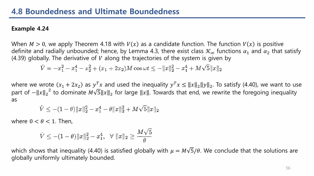
When 𝑀 > 0, we apply Theorem 4.18 with 𝑉 𝑥 as a candidate function. The function 𝑉 𝑥 is positive definite and radially unbounded; hence, by Lemma 4.3, there exist class 𝒦∞ functions 𝛼1 and 𝛼2 that satisfy (4.39) globally. The derivative of 𝑉 along the trajectories of the system is given by
where we wrote 𝑥1 + 2𝑥2 as 𝑦𝑇𝑥 and used the inequality 𝑦𝑇𝑥 ≤ 𝑥 2 𝑦 2. To satisfy (4.40), we want to use
part of − 𝑥 22
to dominate 𝑀 5 𝑥 2 for large 𝑥 . Towards that end, we rewrite the foregoing inequality as
where 0 < 𝜃 < 1. Then,
which shows that inequality (4.40) is satisfied globally with 𝜇 = 𝑀 5/𝜃. We conclude that the solutions are globally uniformly ultimately bounded.
Example 4.24
56

4.8 Boundedness and Ultimate Boundedness
We have to find the functions 𝛼1 and 𝛼2 to calculate the ultimate bound. From the inequalities
we see that 𝛼1 and 𝛼2 can be taken as
Thus, the ultimate bound is given by
Example 4.24
57
4.9 Input-to-State Stability
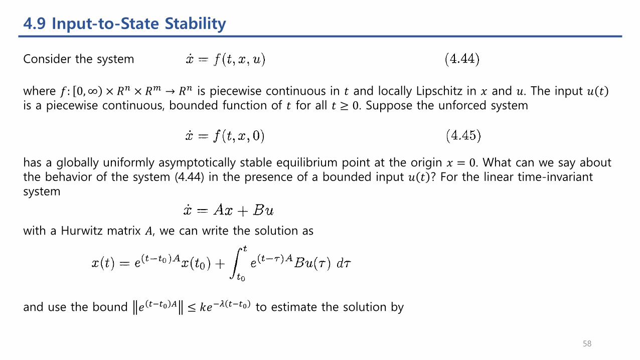
Consider the system
where 𝑓: 0,∞ × 𝑅𝑛 × 𝑅𝑚 → 𝑅𝑛 is piecewise continuous in 𝑡 and locally Lipschitz in 𝑥 and 𝑢. The input 𝑢 𝑡is a piecewise continuous, bounded function of 𝑡 for all 𝑡 ≥ 0. Suppose the unforced system
has a globally uniformly asymptotically stable equilibrium point at the origin 𝑥 = 0. What can we say about the behavior of the system (4.44) in the presence of a bounded input 𝑢 𝑡 ? For the linear time-invariant system
with a Hurwitz matrix 𝐴, we can write the solution as
and use the bound 𝑒 𝑡−𝑡0 𝐴 ≤ 𝑘𝑒−𝜆 𝑡−𝑡0 to estimate the solution by
58
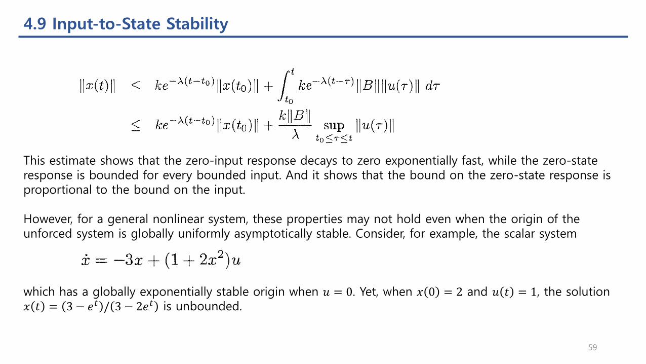
4.9 Input-to-State Stability
This estimate shows that the zero-input response decays to zero exponentially fast, while the zero-state response is bounded for every bounded input. And it shows that the bound on the zero-state response is proportional to the bound on the input.
However, for a general nonlinear system, these properties may not hold even when the origin of the unforced system is globally uniformly asymptotically stable. Consider, for example, the scalar system
which has a globally exponentially stable origin when 𝑢 = 0. Yet, when 𝑥 0 = 2 and 𝑢 𝑡 = 1, the solution 𝑥 𝑡 = 3 − 𝑒𝑡 / 3 − 2𝑒𝑡 is unbounded.
59
4.9 Input-to-State Stability
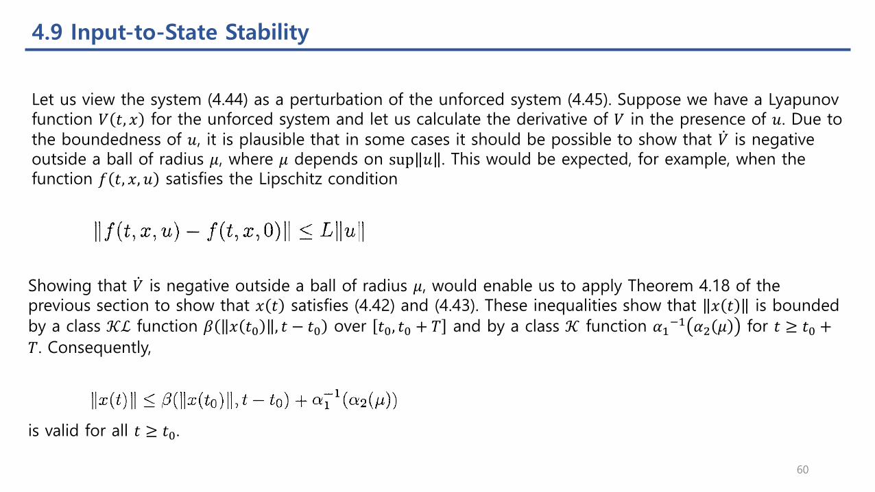
Let us view the system (4.44) as a perturbation of the unforced system (4.45). Suppose we have a Lyapunov function 𝑉 𝑡, 𝑥 for the unforced system and let us calculate the derivative of 𝑉 in the presence of 𝑢. Due to the boundedness of 𝑢, it is plausible that in some cases it should be possible to show that ሶ𝑉 is negative outside a ball of radius 𝜇, where 𝜇 depends on sup 𝑢 . This would be expected, for example, when the function 𝑓 𝑡, 𝑥, 𝑢 satisfies the Lipschitz condition
Showing that ሶ𝑉 is negative outside a ball of radius 𝜇, would enable us to apply Theorem 4.18 of the previous section to show that 𝑥 𝑡 satisfies (4.42) and (4.43). These inequalities show that 𝑥 𝑡 is bounded
by a class 𝒦ℒ function 𝛽 𝑥 𝑡0 , 𝑡 − 𝑡0 over 𝑡0, 𝑡0 + 𝑇 and by a class 𝒦 function 𝛼1−1 𝛼2 𝜇 for 𝑡 ≥ 𝑡0 +
𝑇. Consequently,
is valid for all 𝑡 ≥ 𝑡0.
60
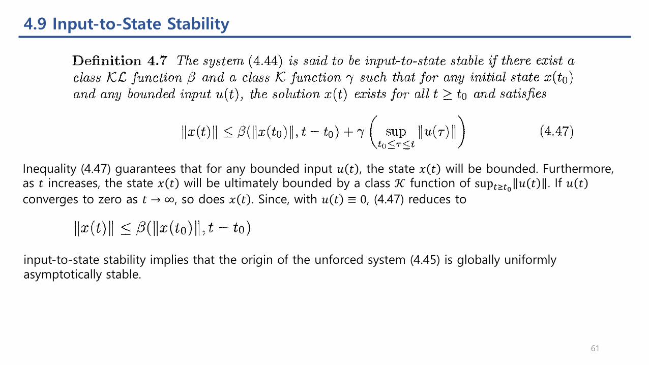
4.9 Input-to-State Stability
Inequality (4.47) guarantees that for any bounded input 𝑢 𝑡 , the state 𝑥 𝑡 will be bounded. Furthermore, as 𝑡 increases, the state 𝑥 𝑡 will be ultimately bounded by a class 𝒦 function of sup𝑡≥𝑡0 𝑢 𝑡 . If 𝑢 𝑡
converges to zero as 𝑡 → ∞, so does 𝑥 𝑡 . Since, with 𝑢 𝑡 ≡ 0, (4.47) reduces to
input-to-state stability implies that the origin of the unforced system (4.45) is globally uniformly asymptotically stable.
61
4.9 Input-to-State Stability
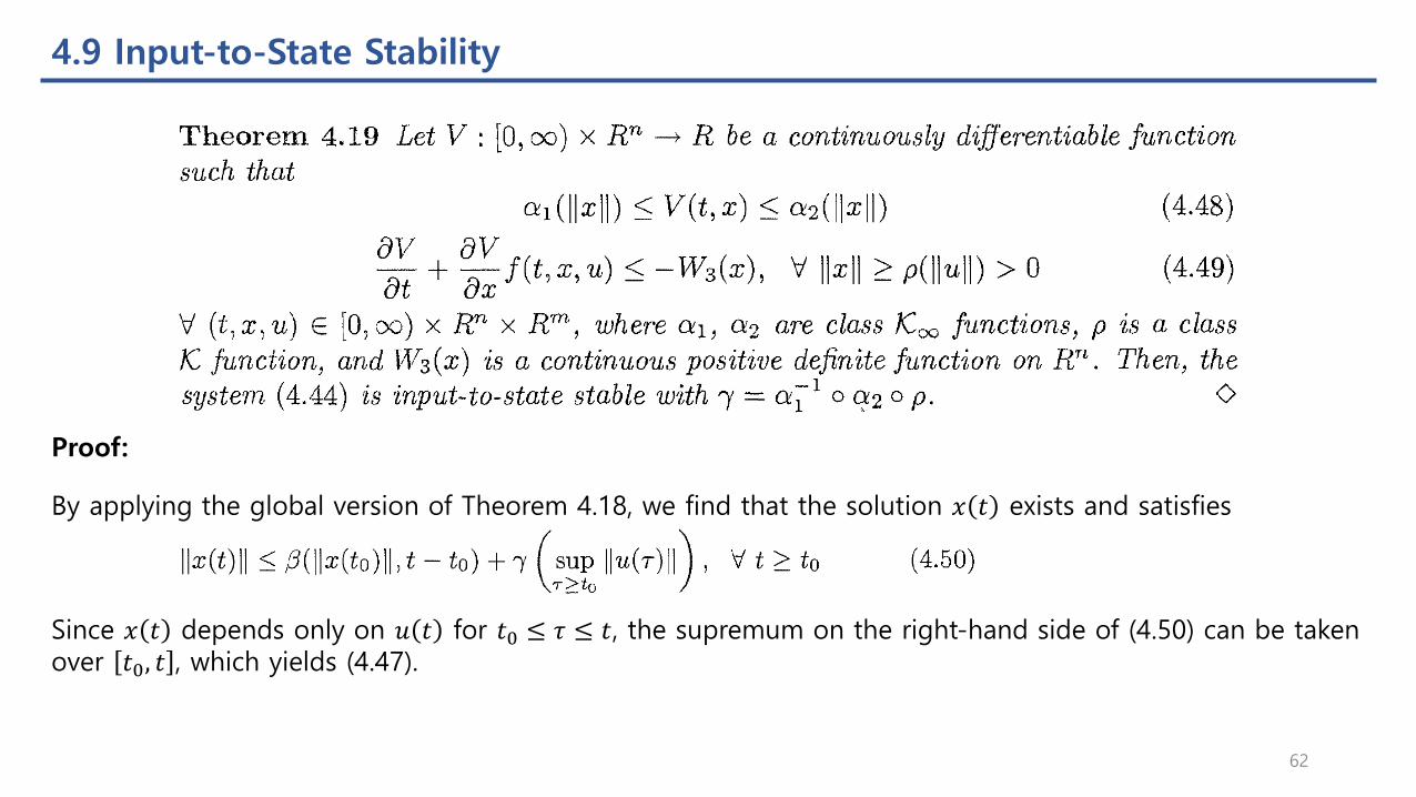
Proof:
By applying the global version of Theorem 4.18, we find that the solution 𝑥 𝑡 exists and satisfies
Since 𝑥 𝑡 depends only on 𝑢 𝑡 for 𝑡0 ≤ 𝜏 ≤ 𝑡, the supremum on the right-hand side of (4.50) can be taken over 𝑡0, 𝑡 , which yields (4.47).
62
4.9 Input-to-State Stability
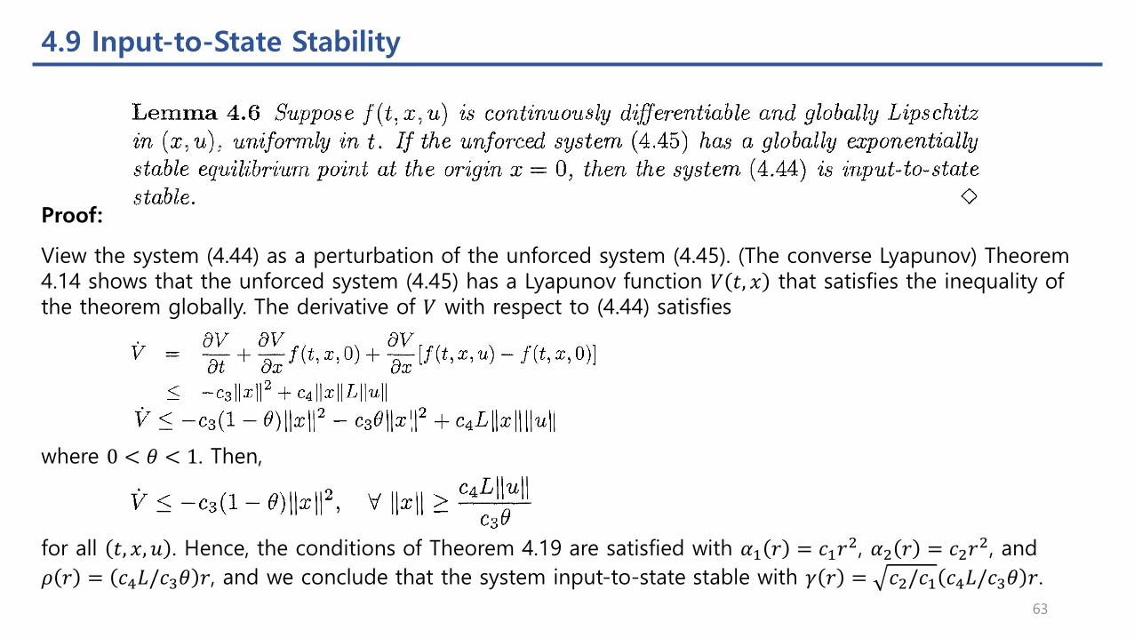
View the system (4.44) as a perturbation of the unforced system (4.45). (The converse Lyapunov) Theorem 4.14 shows that the unforced system (4.45) has a Lyapunov function 𝑉 𝑡, 𝑥 that satisfies the inequality of the theorem globally. The derivative of 𝑉 with respect to (4.44) satisfies
Proof:
where 0 < 𝜃 < 1. Then,
for all 𝑡, 𝑥, 𝑢 . Hence, the conditions of Theorem 4.19 are satisfied with 𝛼1 𝑟 = 𝑐1𝑟2, 𝛼2 𝑟 = 𝑐2𝑟
2, and
𝜌 𝑟 = 𝑐4𝐿/𝑐3𝜃 𝑟, and we conclude that the system input-to-state stable with 𝛾 𝑟 = 𝑐2/𝑐1 𝑐4𝐿/𝑐3𝜃 𝑟.
63

4.9 Input-to-State Stability
Example 4.25
The system
has a globally asymptotically stable origin when 𝑢 = 0. Taking 𝑉 = 𝑥2/2, the derivative of 𝑉 along the trajectories of the system is given by
where 0 < 𝜃 < 1. Thus, the system is input-to-state stable with 𝛾 𝑟 = 𝑟/𝜃 1/3.
Example 4.26
The system
has a globally exponentially stable origin when 𝑢 = 0, but Lemma 4.6 does not apply since 𝑓 is not globally Lipschitz. Taking 𝑉 = 𝑥2/2, we obtain
Thus, the system is input-to-state stable with 𝛾 𝑟 = 𝑟2.
In Examples 4.25 and 4.26, the function 𝑉 𝑥 = 𝑥2/2 satisfies (4.48) with 𝛼1 𝑟 = 𝛼2 𝑟 = 𝑟2/2. Hence,
𝛼1−1 𝛼2 𝑟 = 𝑟 and 𝛾 𝑟 reduces to 𝜌 𝑟 .
64
4.9 Input-to-State Stability
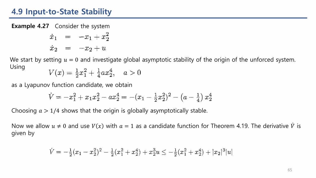
Example 4.27 Consider the system
We start by setting 𝑢 = 0 and investigate global asymptotic stability of the origin of the unforced system. Using
as a Lyapunov function candidate, we obtain
Choosing 𝑎 > 1/4 shows that the origin is globally asymptotically stable.
Now we allow 𝑢 ≠ 0 and use 𝑉 𝑥 with 𝑎 = 1 as a candidate function for Theorem 4.19. The derivative ሶ𝑉 is given by
65
4.9 Input-to-State Stability
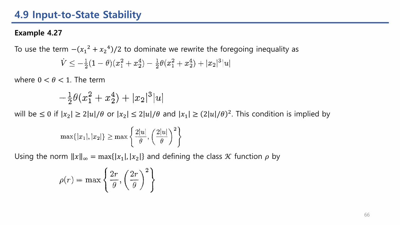
To use the term − 𝑥12 + 𝑥2
4 /2 to dominate we rewrite the foregoing inequality as
where 0 < 𝜃 < 1. The term
Example 4.27
will be ≤ 0 if 𝑥2 ≥ 2 𝑢 /𝜃 or 𝑥2 ≤ 2 𝑢 /𝜃 and 𝑥1 ≥ 2 𝑢 /𝜃 2. This condition is implied by
Using the norm 𝑥 ∞ = max 𝑥1 , 𝑥2 and defining the class 𝒦 function 𝜌 by
66
4.9 Input-to-State Stability
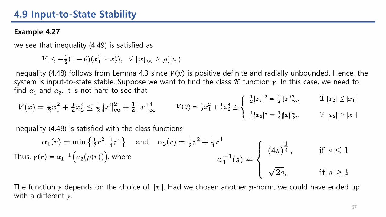
we see that inequality (4.49) is satisfied as
Example 4.27
Inequality (4.48) follows from Lemma 4.3 since 𝑉 𝑥 is positive definite and radially unbounded. Hence, the system is input-to-state stable. Suppose we want to find the class 𝒦 function 𝛾. In this case, we need to find 𝛼1 and 𝛼2. It is not hard to see that
Inequality (4.48) is satisfied with the class functions
Thus, 𝛾 𝑟 = 𝛼1−1 𝛼2 𝜌 𝑟 , where
The function 𝛾 depends on the choice of 𝑥 . Had we chosen another 𝑝-norm, we could have ended up with a different 𝛾.
67

4.9 Input-to-State Stability
An interesting application of the concept of input-to-state stability arises in the stability analysis of the cascade system
where 𝑓1: 0,∞ × 𝑅𝑛1 × 𝑅𝑛2 → 𝑅𝑛1 and 𝑓2: 0,∞ × 𝑅𝑛2 → 𝑅𝑛2 are piecewise continuous in 𝑡 and locally
Lipschitz in 𝑥 =𝑥1𝑥2
. Suppose both
and (4.52) have globally uniformly asymptotically stable equilibrium points at their respective origins. Under what condition will the origin 𝑥 = 0 of the cascade system possess the same property?
68

4.9 Input-to-State Stability
Proof:
Let 𝑡0 ≥ 0 be the initial time. The solutions of (4.51) and (4.52) satisfy
globally, where 𝑡 ≥ 𝑠 ≥ 𝑡0, 𝛽1, 𝛽2 are class 𝒦ℒ functions and 𝛾1 is a class 𝒦 function. Apply (4.53) with 𝑠 =𝑡 + 𝑡0 /2 to obtain
69
4.9 Input-to-State Stability
Proof:
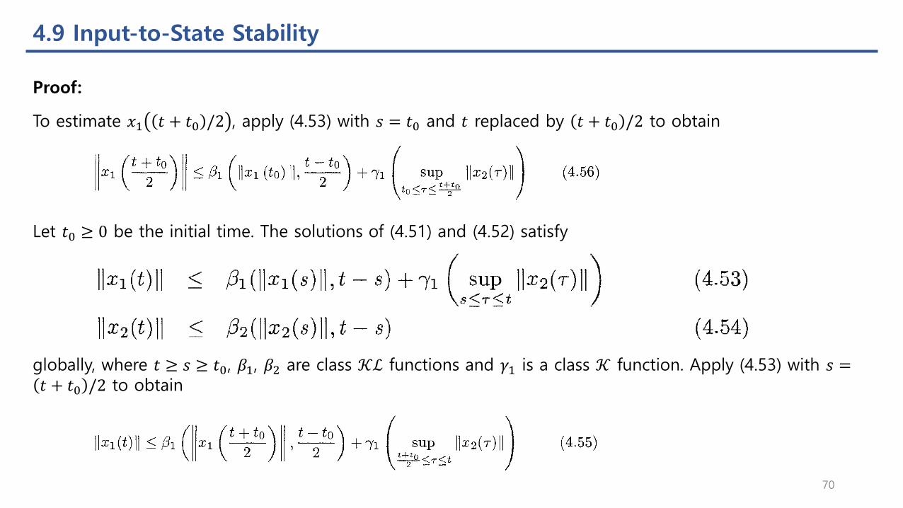
To estimate 𝑥1 𝑡 + 𝑡0 /2 , apply (4.53) with 𝑠 = 𝑡0 and 𝑡 replaced by 𝑡 + 𝑡0 /2 to obtain
Let 𝑡0 ≥ 0 be the initial time. The solutions of (4.51) and (4.52) satisfy
globally, where 𝑡 ≥ 𝑠 ≥ 𝑡0, 𝛽1, 𝛽2 are class 𝒦ℒ functions and 𝛾1 is a class 𝒦 function. Apply (4.53) with 𝑠 =𝑡 + 𝑡0 /2 to obtain
70
4.9 Input-to-State Stability
Proof:
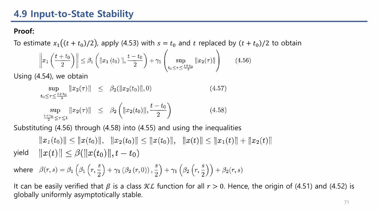
To estimate 𝑥1 𝑡 + 𝑡0 /2 , apply (4.53) with 𝑠 = 𝑡0 and 𝑡 replaced by 𝑡 + 𝑡0 /2 to obtain
Using (4.54), we obtain
Substituting (4.56) through (4.58) into (4.55) and using the inequalities
yield
where
It can be easily verified that 𝛽 is a class 𝒦ℒ function for all 𝑟 > 0. Hence, the origin of (4.51) and (4.52) is globally uniformly asymptotically stable.
71
Related Documents


![Lyapunov Stability Rizki Adi Nugroho [1410501075]](https://static.cupdf.com/doc/110x72/589a2d3a1a28ab051f8b5cbd/lyapunov-stability-rizki-adi-nugroho-1410501075.jpg)