LPF computation revisited

LPF computation revisited⋆

Maxime Crochemore1,4, Lucian Ilie⋆⋆2, Costas S. Iliopoulos1,5,Marcin Kubica3, Wojciech Rytter⋆ ⋆ ⋆3,6, and Tomasz Walen3

1 Dept. of Computer Science, King’s College London, London WC2R 2LS, UK2 Dept. of Computer Science, University of Western Ontario, London,

Ontario, N6A 5B7, Canada3 Institute of Informatics, Warsaw University, ul. Banacha 2,

02-097 Warszawa, Poland4 Universite Paris-Est, France

5 Digital Ecosystems & Business Intelligence Institute, Curtin University ofTechnology, Perth WA 6845, Australia

6 Dept. of Math. and Informatics, Copernicus University, Torun, Poland

Abstract. We present efficient algorithms for storing past segments of atext. They are computed using two previously computed read-only arrays(SUF and LCP) composing the Suffix Array of the text. They computethe maximal length of the previous factor (subword) occurring at eachposition of the text in a table called LPF. This notion is central both inmany conservative text compression techniques and in the most efficientalgorithms for detecting motifs and repetitions occurring in a text.The main results are: a linear-time algorithm that computes explicitlythe permutation that transforms the LCP table into the LPF table; atime-space optimal computation of the LPF table; and an O(n log n)strong in-place computation of the LPF table.Keywords: longest previous factor, suffix array, Ziv-Lempel factorisa-tion, text compression, detection of repetitions.

1 Longest Previous Factor

We consider a string y of length n on the alphabet A: y = y[0 . . n − 1]. Theproblem is to compute the Longest Previous Factor table defined, for 0 ≤ i < n,by

LPF[i] = maxk | y[i . . i + k − 1] occurs at a position j < i.For example, the text y = abaabababbabbb has the following LPF table.

position i 0 1 2 3 4 5 6 7 8 9 10 11 12 13y[i] a b a a b a b a b b a b b b

LPF[i] 0 0 1 3 2 4 3 2 1 4 3 2 2 1

⋆ Research supported in part by the Royal Society, UK.⋆⋆ Research supported in part by NSERC.

⋆ ⋆ ⋆ Supported by grant N206 004 32/0806 of the Polish Ministry of Science and HigherEducation.

The problem may be regarded as an extension of the Ziv-Lempel factorisation(LZ77) of a string as defined in [20]. A string y is decomposed into factors, calledphrases, u0, u1, . . . , uk, for which y = u0u1 · · ·uk and defined informally by:ui = va where a is a letter and v is the longest segment of u0u1 · · ·ui occurringboth at position |u0u1 · · ·ui−1| and before it in y. The factorisation is used inseveral adaptive compression methods which encode carefully re-occurrences ofphrases by pointers or integers (see [18] or [19]). The factorisation yields morepowerful compressors than the factorisation in [21] (called LZ78) where a phraseis an extension by a single letter of a previous phrase. But the LZ77 factorisationis more difficult to compute.

It is clear that the LZ77 factorisation comes readily when the LPF table isavailable, which is a remarkable application of the table (see [5]). This implies alinear-time solution for LZ77 factorisation on integer alphabets. Previous solu-tions using a Suffix Tree [17] or a Suffix Automaton [2] of the text not only runin time O(|y| log |A|) but these data structures are more space-expensive thanthe Suffix Array.

A slight variant of string parsing, whose relation with the LZ77 factorisationis analysed in [1], plays an important role in String Algorithms. The intuitivereason is that, when processing a string on-line, the work done on an elementof the factorisation can usually be skipped because already done on one of itsprevious occurrences. A typical application of this idea resides in algorithms tocompute repetitions in strings (see [2, 15, 14]). For example, the algorithm in [14]reports all maximal repetitions (called runs) occurring in a string in O(|y| log |A|)time. It runs in linear time if a Suffix Array is used instead of a Suffix Tree [4].Indeed the technique seems to be the only technique that leads to linear-timealgorithms independently of the alphabet size for this type of question.

Suffix Arrays provide an ideal data structure to solve many questions requir-ing an index on all the factors of a string. Introduced by Manber and Myers [16]the structure can be built in linear-time by different methods [10, 12, 13, 8] forsorting the suffixes of the text possibly adding the method of [11] to computethe Longest Common Prefix table. The result holds if the text is drawn from aninteger alphabet, that is, if the alphabet of the text can be sorted in linear time(otherwise the Ω(n log n) lower bound for sorting applies).

The notion of Longest Previous Factor has been introduced by Franek et al.as part of their concept of a Quasi Suffix Array (their π array is the LPF table)in [7], where the authors presented a direct computation running in O(n log n)average time. A naive computation of the LPF table, either on the text itself oron its Suffix Array, as done by the algorithm LPF-naive in Section 5, leads toquadratic effective running time on many inputs.

In this article we intensively use the Suffix Array of the text to be processed,and we consider only linear-time solutions. A graphical representation of the Suf-fix Array structure helps understand the design of the algorithms. The LongestPrevious Factor is coined in [4], where a linear-time computation is describedand applied to LZ77 factorisation. Another version running on-line on the SuffixArray of the text and requiring only O(

√n) extra memory space is shown in [5].

We improve on the previous results and show that the computation of theLongest Previous Factor table of a text from its Suffix Array can be implementedto run in linear time with only a constant amount of additional memory space.Thus, the method is time-space optimal.

The next section introduces the necessary material for the design of LongestPrevious Factor computations. First, an algorithm similar to the one in [4] isdescribed. The algorithm is regarded in Section 3 as using the Suffix Array likea sorting network. Section 4 shows how the computation can be done on-line onthe Suffix Array and Section 5 describes the time-space optimal algorithm forconstructing the table.

2 Using a Suffix Array

The Suffix Array of the text y is a data structure used for indexing its content.It comprises two tables that we denote SUF and LCP and that are defined asfollows.

The table SUF stores the list of position on y associated with the sorted listof its suffixes in increasing lexicographic order. That is, the table is such that

y[SUF[0] . . n− 1] < y[SUF[1] . . n− 1] < · · · < y[SUF[n− 1] . . n− 1].

Thus, indices on SUF are ranks of the suffixes in their sorted list.The second table LCP is also indexed by the ranks of suffixes and stores

the longest common prefixes between consecutive suffixes in the sorted list. Letlcp(i, j) = longest common prefix of y[i . . n − 1] and y[j . . n − 1], for two posi-tions i and j on y. Then, LCP[0] = 0 and, for 0 < r < n, we set

LCP[r] = |lcp(SUF[r − 1], SUF[r])|.

(The actual Suffix Array contains indeed about n additional LCP values usedfor binary searching the suffixes.)

Example 1. For the text y = abaabababbabbb we get the Suffix Array:

rank r 0 1 2 3 4 5 6 7 8 9 10 11 12 13SUF[r] 2 0 3 5 7 10 13 1 4 6 9 12 8 11LCP[r] 0 1 3 4 2 3 0 1 2 3 4 1 2 2

The computation of the Suffix Array of y can be done in time O(n log n) inthe comparison model [16] (see [3, 6, 9]). If the text is on an alphabet of integersin the range [0, nc] for some constant c, the Suffix Array can be built in timeO(n) [10, 12, 13, 8] (see also [3]).

Graphic representation The Suffix Array of the text y has a nice graphic repre-sentation that helps understand the algorithms computing the LPF table. Theabscissae axis refers to ranks of suffixes and the ordinates axis refers to their po-sitions. The sorted list of suffixes is plotted by their positions, and consecutivepositions are linked by an edge whose label is the associated LCP value. Figure 1shows the Suffix Array representation for the text of Example 1.

0 1 2 3 4 5 6 7 8 9 10 11 12 13 140

1

2

3

4

5

6

7

8

9

10

11

12

13

14

ranks of suffixes

posi

tions

ofsu

ffixes

2

0

3

5

7

10

13

1

4

6

9

12

8

11

1

3

4

2

3

0

1

2

3

4

1 22

Fig. 1. Graph of the permutation of positions on abaabababbabbb (Example 1) in thelexicographic order of its suffixes. Labels of edges are Longest Common Prefix lengthsbetween consecutive suffixes.

Simple algorithm The LCP table satisfies a simple property consequence of thelexicographic order: the LCP value between two positions at ranks r and t, r < t,is the minimal value in LCP[r + 1 . . t].

For a rank r, let us define prev[r] as the largest rank s, s < r, for whichSUF[s] < SUF[r] if it exists, and as −1 otherwise. Let us also define the dualnotion next[r] as the smallest rank t, r < t, for which SUF[t] < SUF[r] if it exists,and as n otherwise. The above property implies that to compute LPF[SUF[r]]there is no need to look at ranks smaller than prev[r] or greater than next[r],that is

LPF[SUF[r]] = max |lcp(SUF[r], SUF[prev[r]])|, |lcp(SUF[r], SUF[next[r]])| (1)

where undefined LCP values are set to 0. In particular, if a position i is a “peak”at rank r in the graphic representation of the Suffix Array (SUF[r] = i) we get

LPF[i] = maxLCP[r], LCP[r + 1].

And the minimum of the two values is the LCP between positions at ranks r−1and r + 1 if defined. This gives the idea underlying the next algorithm.

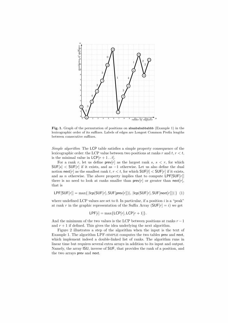
Figure 2 illustrates a step of the algorithm when the input is the text ofExample 1. The algorithm LPF-simple computes the two tables prev and next,which implement indeed a double-linked list of ranks. The algorithm runs inlinear time but requires several extra arrays in addition to its input and output.Namely, the array ISU, inverse of SUF, that provides the rank of a position, andthe two arrays prev and next.

0 1 2 3 4 5 6 7 8 9 10 11 12 13 140

1

2

3

4

5

6

7

8

9

10

11

12

13

14

ranks of suffixes

posi

tions

ofsu

ffixes

2

0

3

5

7

10

13

1

4

6

9

12

8

11

1

3

4

2

3

0

1

2

3

4

1 22

0

0

1

Fig. 2. Illustration of the run of the algorithm LPF-simple on the text abaabababbabbb(see Figure 1) after processing positions 13, 12, 11, 10. Gray positions and gray edgesare no longer considered. The next step is to process position 9 at rank 10. Accordingto the weights of edges pending from 9, we have LPF[9] = max4, 1 = 4. Positions 6and 8 will be linked, through the prev and next arrays on their ranks, with an edge ofweight min4, 1 = 1, which is indeed LPF[8].

LPF-simple(SUF, LCP, n)

1 LCP-copy← LCP

2 LCP-copy[n]← 03 ISU← inverse SUF

4 for r← 0 to n− 1 do

5 prev[r]← r − 16 next[r]← r + 17 for i← n− 1 downto 0 do

8 r ← ISU[i]9 LPF[i]← maxLCP-copy[r], LCP-copy[next[r]]

10 LCP-copy[next[r]]← minLCP-copy[r], LCP-copy[next[r]]11 if prev[r] ≥ 0 then

12 next[prev[r]]← next[r]13 if next[r] < n then

14 prev[next[r]]← prev[r]15 return LPF

Proposition 1. The algorithm LPF-simple computes the LPF array of a textof length n from its Suffix Array in linear time and space. It requires 3n + cinteger cells in addition to its input and output.

The array next can alternatively be pre-computed by the following procedurewhose linear-time behaviour is an interesting exercise left to the reader. Theprocedure also computes the array LPF> defined in [4] and that accounts forlarger ranks only. It is defined, for r = 0, . . . , n− 1, by

LPF>[r] = |lcp(SUF[r], SUF[next[r]])|.

Next(SUF, LCP, n)

1 next[n− 1]← n2 LPF>[n− 1]← 03 for r← n− 2 downto 0 do

4 t← r + 15 ℓ← LCP[t]6 while t < n and SUF[t] > SUF[r] do

7 ℓ← minℓ, LPF>[t]8 t← next[t]9 next[r]← t

10 LPF>[r]← ℓ11 return next, LPF>

The computation of the dual prev and LPF< arrays is done symmetrically.When both arrays LPF< and LPF> are available, the computation of the LPF

table is an application of identity 1 that rewrites, for position i at rank r, as

LPF[i] = max(LPF>[r], LPF<[r]).

3 Sorting network

It has been noticed in [4] that the content of the LPF table is the same asthat of the LCP table up to some permutation. A question arises then: whatpermutation is it? Does it depend on the text, its Suffix Array or maybe just itsLCP array? It turns out that, for fixed SUF and LCP arrays, it does not dependon the actual text. It is possible to construct such a sorting network, whose shapedepends only on the Suffix Array, that transforms the LCP array into the LPF

table. This observation leads to the algorithm LPF-sorting, producing LPF bypermutating the elements of LCP.

In the algorithm LPF-sorting below we assume that the table next intro-duced in the previous section has been pre-computed by the procedure Next

(in which instructions related to LPF> are useless and may be removed, as wellas the parameter LCP). Table next is used to compute, for each position i, thenext closest position nextp[i] in the Suffix Array that is smaller than i, that is,

nextp[SUF[r]] = SUF[mint | t > r and SUF[t] < SUF[r]].

Initially, the LPF table is a copy of the LCP array permuted according to theSUF table. The algorithm sorts the array by permuting its elements to get theLPF table.

LPF-sorting(SUF, LCP, n)

1 SUF[n]← −12 for r← 0 to n− 1 do

3 LPF[SUF[r]]← LCP[r]4 nextp[SUF[r]]← SUF[next[r]]5 for i← n− 1 downto 0 do

6 if (nextp[i] ≥ 0) and (LPF[i] < LPF[nextp[i]]) then

7 Exchange(LPF[i], LPF[nextp[i]])8 return LPF

Note that the elements of LPF are exchanged (lines 6–7) only if they are notin increasing order. Which elements are compared, depends on values in nextp,and this in turn depends only on the Suffix Array. So, for a given Suffix Array,one can construct a sorting network implementing lines 5–7 of the algorithmLPF-sorting. Hence, the following proposition holds:

Proposition 2. For a given Suffix Array of a text, there exists a sorting networkprocessing a sequence of n numbers in such a way that it transforms the LCP

table into the LPF table. Moreover, the shape of the sorting network depends onlyon the Suffix Array, but not on its LCP table nor on the actual text.

As it is done for any sorting procedure, instead of directly computing theLPF table, the algorithm LPF-sorting can equivalently produce explicitly thepermutation π to transform the LCP array into the LPF table, that is, the per-mutation that satisfies LPF[i] = LCP[π[i]].

The algorithm LPF-sorting uses only one integer array in addition to itsinput and output since the next table it uses is substituted for the nextp table.This yields the next statement.

Proposition 3. The algorithm LPF-sorting computes the LPF table of a textof length n from its Suffix Array in linear time and space. It requires n+c integercells in addition to its input and output.

4 On-line computation

Techniques of the previous sections to compute the LPF table are simple butspace consuming. In this section and the next one we address this issue. Weshow that a computation on-line on the Suffix Array using a stack reduces thememory space to only O(

√n) for a text of length n.

The design of the on-line computation still relies on the property used forthe algorithm of Section 2 and related to “peaks” (see lines 6-8 below). It re-lies additionally on another straightforward property that we describe now. As-sume that a position SUF[r] at rank r satisfies LCP[r] ≥ LCP[r + 1]. Then, noposition after it in the list can provide a larger LCP value and therefore weget LPF[SUF[r]] = LCP[r]. This is implemented in lines 10-11 of the algorithmLPF-on-line.

Note that lines 15 to 18 may be removed from the algorithm LPF-on-line

if the Suffix Array can be extended to rank n and initialised to SUF[n] = −1and LCP[n] = 0. But we prefer the present design that is compatible with thealgorithm of the next section.

LPF-on-line(SUF, LCP, n)

1 EmptyStack(S)2 for r← 0 to n− 1 do

3 r-lcp← LCP[r]4 while not Empty(S) do

5 (t, t-lcp)← Top(S)6 if SUF[r] < SUF[t] then

7 LPF[SUF[t]]← maxt-lcp, r-lcp8 r-lcp← mint-lcp, r-lcp9 Pop(S)

10 elseif (SUF[r] > SUF[t]) and (r-lcp ≤ t-lcp) then

11 LPF[SUF[t]]← t-lcp12 Pop(S)13 else break14 Push(S, (r, r-lcp))15 while not Empty(S) do

16 (t, t-lcp)← Top(S)17 LPF[SUF[t]]← t-lcp18 Pop(S)19 return LPF

Stack size The extra memory space used by the algorithm LPF-on-line tocompute the LPF table of a text is occupied by the stack and a constant numberof integer variables. To evaluate the total size required by the algorithm it isthen important to determine the maximal size of the stack for a text of lengthn. It is proved in [5] that this quantity is O(

√n).

For most values of n there are plenty of texts for which the stack reachesits maximal size. But if n is of the form k(k + 1)/2, that is, if it is the sum ofthe first k positive integers, then there is a unique string on the alphabet a, b(with a < b) giving the maximal size stack. This word is aabab

2 · · · abk−1 andthe maximal stack size is k.

The next table shows maximal stack sizes for texts of lengths 4 to 19:

length n 4 5 6 7 8 9 10 11 12 13 14 15 16 17 18 19 20 21 22max-stack-size 2 2 3 3 3 3 4 4 4 4 4 5 5 5 5 5 5 6 6

Proposition 4. The algorithm LPF-on-line computes the LPF array of a textof length n from its Suffix Array in linear time and O(

√n) space. It requires less

than 2√

2n + c integer cells in addition to its input and output.

5 Time-space optimal implementation

In this section we show that the computation of the LPF table of a text can beimplemented with only constant memory space in addition to the Suffix Arrayof the text and its LPF table. The underlying property used for this purpose isthe O(

√n) stack size reported in the previous section. The property allows an

implementation of the stack inside the LPF table for a sufficiently large part ofthe text. The rest of the computation for the remaining positions is done in amore time-expensive manner but for a small part of the text. This preserves thelinear running time of the whole computation.

LPF-optimal(SUF, LCP, n)

1 ⊲ it is assumed that n ≥ 8

2 K ← ⌊n− 2√

2n⌋3 ⊲ next three procedures share the same LPF table4 LPF-on-line(SUF, LCP, K)5 LPF-naive(SUF, LCP, K, n)6 LPF-anchored(SUF, LCP, K, n)7 return LPF

It is rather clear that only constant extra memory space is required to imple-ment the strategy retained by the algorithm LPF-optimal. The choice of theparameter K is a result of the previous section and is done to let enough spacein the LPF array to implement the stack used by the algorithm LPF-on-line.

Although not done here, the choice of the parameter K can be dynamic anddone during the algorithm LPF-on-line as n − 2k − 1, where k is the size ofthe stack just before executing line 15. This certainly reduces the actual runningtime but does not improve its asymptotic evaluation.

In the algorithm LPF-optimal, the stack of the procedure LPF-on-line

is implemented in the LPF table. Access to the table is done via the SUF array.Doing so, the stack is treated like a continuous space LPF[SUF[K . . n − 1]]. El-ements are stored sequentially so that the elementary stack operations (empty,top, push, pop) are all executed in constant time. Therefore, the running timeof the first step is O(n) (indeed O(K)) as for the algorithm LPF-on-line.

Example 2. The next table shows the content of the LPF array at two stagesof the run of the procedure LPF-on-line on Example 1: (i) immediately afterprocessing rank 5 and (ii) at the end of the first step.

rank r 0 1 2 3 4 5 6 7 8 9 10 11 12 13(i) LPF[SUF[r]] 1 3 4 5 3 4 2 1 0(ii) LPF[SUF[r]] 1 0 3 4 2 3 1 8 2 7 0

Row (i) shows that LPF values of positions 2, 3, 5 at respective ranks 0, 2,3 have already been computed. The part LPF[SUF[8 . . 13]] of the table storesthe content of the stack: ((1, 0), (4, 2), (5, 3)). Row (ii) shows that values havealready been computed for positions at ranks 0 to 6. The content of the stack is((7, 0), (8, 2)). On this example, K could have been set dynamically to 5.

Naive computation The second step of the algorithm LPF-optimal processesthe Suffix Array from rank K. For each rank r, the values prev[r], next[r] andthe corresponding LCP values are computed starting from r and going backwardand forward, respectively. The code is given below for the sake of completenessbut it contains no algorithmic high value.

The process takes O(n−K) time per rank, and hence the total running timeof the step is O((n−K)2), which is O(n) since K = n− 2

√2n.

LPF-naive(SUF, LCP, K, n)

1 LCP[n]← 02 for r← K to n− 1 do

3 left ← LCP[r]4 s← r − 15 while s ≥ K and SUF[s] > SUF[r] do

6 left ← minleft , LCP[s]7 s← s− 18 if s = K − 1 then

9 left ← 010 t← r + 111 right ← LCP[t]12 while t < n and SUF[t] > SUF[r] do

13 t← t + 114 right ← minright , LCP[t]15 LPF[SUF[r]]← maxleft , right16 return LPF

Completing the computation The first two steps of the algorithm LPF-optimal

process independently two segments of the Suffix Array. The last step consistsin joining their results, which requires updating some LPF values. Indeed, for arank r, r < K, next[r] can be in [K, n−1], which implies that the computation ofLPF[SUF[r]] might not be achieved. The same phenomenon happens for a rankin the second part, whose associated prev rank is smaller than K.

The next algorithm updates all LPF values and completes the whole com-putation. It assumes that the LPF calculation has been done independently onparts LPF[SUF[0 . .K−1]] and LPF[SUF[K . . n−1]] of the array, which is realisedby the first two steps on the algorithm LPF-optimal.

The running time of this last step LPF-anchored is obviously linear, O(n),as are the other steps of the algorithm LPF-optimal.

The first conclusion of the section is the following statement.

Theorem 1. The Longest Previous Factor table of a text of length n on aninteger alphabet can be built from its Suffix Array in time O(n) (independentlyof the alphabet size) with a constant amount of extra memory space.

LPF-anchored(SUF, LCP, K, n)

1 s← K − 12 t← K3 ℓ← LCP[K]4 while (s ≥ 0) and (t < n) do

5 ⊲ invariant: ℓ = min LCP[s + 1, . . . , r]6 if SUF[s] < SUF[t] then

7 LPF[SUF[t]]← maxLPF[SUF[t]], ℓ8 t← t + 19 ℓ← minℓ, LCP[t]

10 else LPF[SUF[s]]← maxLPF[SUF[s]], ℓ11 ℓ← minℓ, LCP[s]12 s← s− 113 return LPF

The algorithm LPF-optimal uses the Suffix Array of the input text in aread-only manner but does not use the LPF table in a write-only manner. If thislast condition is to be satisfied, the question remains of whether there exists alinear-time LPF table construction running with constant extra space. We getthis feature if the algorithm LPF-anchored is applied recursively by dividingthe Suffix Array into two equal parts. The running time becomes O(n log n) inthe model of computation allowing priority writes.

Theorem 2. The Longest Previous Factor table of a text of length n on aninteger alphabet can be built from its read-only Suffix Array in time O(n log n)(independently of the alphabet size) with a constant amount of extra memoryspace and with a write-only output.

Despite the use of the output as auxiliary storage in the ultimate linear-timealgorithm, the series of algorithms described in the article provide a large rangeof efficient solutions that meet many practical needs.

6 Acknowledgements

Authors warmly thank German Tischler for his careful inspection of the algo-rithms described in the article.

References

1. J. Berstel and A. Savelli. Crochemore factorization of Sturmian and other infinitewords. In R. Kralovic and P. Urzyczyn, editors, Mathematical Foundations of

Computer Science, volume 4162 of Lecture Notes in Computer Science, pages 157–166. Springer, 2006.

2. M. Crochemore. Transducers and repetitions. Theoretical Computer Science,45(1):63–86, 1986.

3. M. Crochemore, C. Hancart, and T. Lecroq. Algorithms on Strings. CambridgeUniversity Press, Cambridge, UK, 2007. 392 pages.

4. M. Crochemore and L. Ilie. Computing Longest Previous Factor in linear time andapplications. Inf. Process. Lett., 106(2):75–80, 2008.

5. M. Crochemore, L. Ilie, and W. F. Smyth. A simple algorithm for computing theLempel-Ziv factorization. In J. A. Storer and M. W. Marcellin, editors, 18th Data

Compression Conference, pages 482–488. IEEE Computer Society, Los Alamitos,CA, 2008.

6. M. Crochemore and W. Rytter. Jewels of Stringology. World Scientific Publishing,Hong-Kong, 2002. 310 pages.

7. F. Franek, J. Holub, W. F. Smyth, and X. Xiao. Computing quasi suffix arrays.Journal of Automata, Languages and Combinatorics, 8(4):593–606, 2003.

8. G. Nong, S. Zhang, and W. H. Chan. Linear Time Suffix Array Construction UsingD-Critical Substrings, In G. Kucherov and E. Ukkonen, editors, Combinatorial

Pattern Matching, volume 5577 of Lecture Notes in Computer Science, pages 54–67. Springer, 2009.

9. D. Gusfield. Algorithms on Strings, Trees and Sequences: Computer Science and

Computational Biology. Cambridge University Press, Cambridge, UK, 1997. 534pages.

10. J. Karkkainen and P. Sanders. Simple linear work suffix array construction. InJ. C. M. Baeten, J. K. Lenstra, J. Parrow, and G. J. Woeginger, editors, Automata,

Languages and Programming, volume 2719 of Lecture Notes in Computer Science,pages 943–955. Springer, 2003.

11. T. Kasai, G. Lee, H. Arimura, S. Arikawa, and K. Park. Linear-time longest-common-prefix computation in suffix arrays and its applications. In Combinatorial

Pattern Matching, volume 2089 of Lecture Notes in Computer Science, pages 181–192. Springer, 2001.

12. D. K. Kim, J. S. Sim, H. Park, and K. Park. Linear-time construction of suf-fix arrays. In Combinatorial Pattern Matching, volume 2676 of Lecture Notes in

Computer Science, pages 186–199. Springer, 2003.13. P. Ko and S. Aluru. Space efficient linear time construction of suffix arrays. In

Combinatorial Pattern Matching, volume 2676 of Lecture Notes in Computer Sci-

ence, pages 200–210. Springer, 2003.14. R. M. Kolpakov and G. Kucherov. Finding maximal repetitions in a word in linear

time. In FOCS, pages 596–604, 1999.15. M. G. Main. Detecting leftmost maximal periodicities. Discret. Appl. Math.,

25:145–153, 1989.16. U. Manber and G. Myers. Suffix arrays: a new method for on-line string searches.

SIAM J. Comput., 22(5):935–948, 1993.17. M. Rodeh, V. R. Pratt, and S. Even. Linear algorithm for data compression via

string matching. J. ACM, 28(1):16–24, 1981.18. J. Storer and T. Szymanski. Data compression via textual substitution. J. ACM,

29(4):928–951, 1982.19. I. Witten, A. Moffat, and T. Bell. Managing Gigabytes. Van Nostrand Reinhold,

New York, 1994.20. J. Ziv and A. Lempel. A universal algorithm for sequential data compression.

IEEE Transactions on Information Theory, 23(3):337–343, 1977.21. J. Ziv and A. Lempel. Compression of individual sequences via variable-rate coding.

IEEE Transactions on Information Theory, 24(5):530–536, 1978.