Low Complexity DFT-Domain Noise PSD Tracking Using High-Resolution Periodograms

Hindawi Publishing CorporationEURASIP Journal on Advances in Signal ProcessingVolume 2009, Article ID 925870, 15 pagesdoi:10.1155/2009/925870

Research Article

Low Complexity DFT-Domain Noise PSD Tracking UsingHigh-Resolution Periodograms

Richard C. Hendriks,1 Richard Heusdens,1 Jesper Jensen (EURASIP Member),2

and Ulrik Kjems2

1 Department of Mediamatics, Delft University of Technology, Mekelweg 4 2628 CD Delft, The Netherlands2 Oticon A/S, 2765 Smørum, Denmark

Correspondence should be addressed to Richard C. Hendriks, [email protected]

Received 18 February 2009; Revised 16 June 2009; Accepted 26 August 2009

Recommended by Soren Jensen

Although most noise reduction algorithms are critically dependent on the noise power spectral density (PSD), most proceduresfor noise PSD estimation fail to obtain good estimates in nonstationary noise conditions. Recently, a DFT-subspace-based methodwas proposed which improves noise PSD estimation under these conditions. However, this approach is based on eigenvaluedecompositions per DFT bin, and might be too computationally demanding for low-complexity applications like hearing aids.In this paper we present a noise tracking method with low complexity, but approximately similar noise tracking performance asthe DFT-subspace approach. The presented method uses a periodogram with resolution that is higher than the spectral resolutionused in the noise reduction algorithm itself. This increased resolution enables estimation of the noise PSD even when speechenergy is present at the time-frequency point under consideration. This holds in particular for voiced type of speech sounds whichcan be modelled using a small number of complex exponentials.

Copyright © 2009 Richard C. Hendriks et al. This is an open access article distributed under the Creative Commons AttributionLicense, which permits unrestricted use, distribution, and reproduction in any medium, provided the original work is properlycited.

1. Introduction

The growing interest in mobile digital speech processingdevices for both human-to-human and human-to-machinecommunication has led to an increased use of these devices innoisy conditions. In such conditions, it is desirable to applynoise reduction as a preprocessing step in order to extend theSNR range in which the performance of these applications issatisfactory.

A group of methods that is often used for noise reductionin the single-microphone setup are the so-called discreteFourier transform (DFT) domain-based approaches. Thesemethods work on a frame-by-frame basis where the noisysignal is divided in windowed time-frames, such that bothquasistationarity constraints imposed by the input signaland delay constraints imposed by the application at handare satisfied. Subsequently, these windowed time-framesare transformed using a DFT. From the resulting noisyspeech DFT coefficients the corresponding clean speechDFT coefficients are estimated, typically by using Bayesianestimators [1] followed by an inverse DFT to the time

domain and an overlap-add procedure to synthesize theenhanced signal.

Typically, clean speech DFT estimators depend on thespeech and noise power spectral density (PSD), for example,[2–5]. Since these two quantities are defined in terms of thestatistical expectation operator they are unknown in practiceand have to be estimated from the noisy speech signal. Thespeech PSD is often estimated by exploiting the so-calleddecision-directed approach [2]. This method is sometimesfavored over maximum likelihood estimation of the speechPSD [2], because it results in a lower amount and morenatural sounding residual noise [6]. Accurate noise PSDestimation is also of vital importance in order to obtain anestimated clean speech signal with good quality. Errors in thenoise PSD estimate influence directly the amount of achievednoise suppression. Specifically, an overestimate of the noisePSD will typically lead to oversuppression of the noise andpotentially to a loss of speech quality, while an underestimateof the noise PSD leaves an unnecessary amount of residualnoise in the enhanced signal.

2 EURASIP Journal on Advances in Signal Processing

Speech estimatorwindowing

Segmentation &

windowing

Segmentation &

Speech PSDestimator

Noise PSDestimator

DFT

IDFT

HR-DFT

Overlap-

add

Proposed scheme for noise tracking

yt yt(i)

yt,HR(i)

y(k, i)

K

K

K

K

Q Q

σ2X (k, i)

σ2N (k, i)

z−1

yHR(q, i) |yHR(q, i)|2| · |2

x(k, i)

xt(i)

xt

Figure 1: Overview of a DFT-domain-based noise reduction system with the proposed noise PSD tracking algorithm.

Under rather stationary noise conditions, the use of avoice activity detector [7, 8] (VAD) can be sufficient forestimation of the noise PSD. With a VAD the noise PSD isestimated during speech pauses. However, VAD based noisePSD estimation fails when the noise is non-stationary. Analternative is to estimate the noise PSD using algorithmsbased on minimum statistics [9, 10] (MS). These methodsdo not rely on the explicit use of a VAD, but make use of thefact that the power level of the noisy signal in a particularfrequency bin seen across a sufficiently long time intervalwill reach the noise-power level. From the minimum value insuch a time-interval the noise PSD is estimated by applyingan appropriate bias compensation [11]. A crucial parameterin MS based noise PSD estimation is the length of the time-interval. If the interval is chosen too short, speech energywill leak into the noise PSD estimate, because the intervalwill not contain a noise-only region. However, increasing theduration of the interval will increase the tracking delay inregions where the noise PSD is increasing in level.

Another method that does not depend on a VADis quantile-based (QB) noise PSD estimation [12]. Thismethod relies on estimation of the noise PSD by computingper DFT bin a temporal quantile p of noisy periodogramsin a certain time-interval. For the special case of a p = 0.5quantile, the noise PSD is estimated by the median of thedata in the time-interval. The speed at which this methodcan estimate the noise PSD for nonstationary noise sourcesdepends on the length of the time-interval. As such, QB noisePSD estimation methods are subject to a similar tradeoff

as MS. Since the noise PSD estimate is based on a quantileacross time and not only on the minimum, QB noise PSDestimation is expected to track decreasing noise levels withlarger delay than MS, while an increasing noise level canpotentially be tracked faster than MS. In addition, it isalso more likely that QB noise PSD estimation is subjectto leakage of speech into the noise PSD estimate because itexploits the quantile instead of the minimum within a time-interval.

Other recent advancements for noise PSD estimationcomprise data-driven noise PSD estimation [13], improved

minima controlled recursive averaging [14], noise PSDestimation based on classified codebooks [15], and noisePSD estimation based on harmonic tunnelling [16]. Theapproach based on harmonic tunnelling makes explicit useof the harmonic structure in voiced speech sounds andestimates the noise PSD by exploiting the gaps betweenharmonics. Consequently, this method can continuouslyupdate the noise PSD under the condition that the DFT binunder consideration does not contain a speech harmonic.

Recently, in [17], a method for noise tracking was pro-posed which exploits the tonal structure in speech, but whichcan also estimate the noise PSD when speech is actuallypresent in the DFT bin under consideration. This method,named DFT-subspace approach, is based on the constructionof correlation matrices in the DFT-domain for each time-frequency point. These correlation matrices are decomposedusing an eigenvalue decomposition into two submatrices ofwhich the columns span two mutually orthogonal vectorspaces, namely, a noisy signal subspace and a noise-onlysubspace. The eigenvalues that describe the energy in thenoise-only subspace then allow for an update of the noisePSD, even when speech is present. Although the methodproposed in [17] has been shown to be effective for noise PSDestimation and can be implemented in MATLAB in real-timeon a modern PC, the necessary eigenvalue decompositionsmight be too complex for applications with very low-complexity constraints like portable communication devicessuch as mobile phones and hearing aids.

A possible way to reduce the computational complexityof the algorithm in [17] is to use subspace trackingalgorithms that are able to track subspaces efficiently overtime, for example, [18, 19]. Although this might reduce thecomputational complexity of the DFT-subspace algorithm, itmight also change its performance in an unpredictable way.

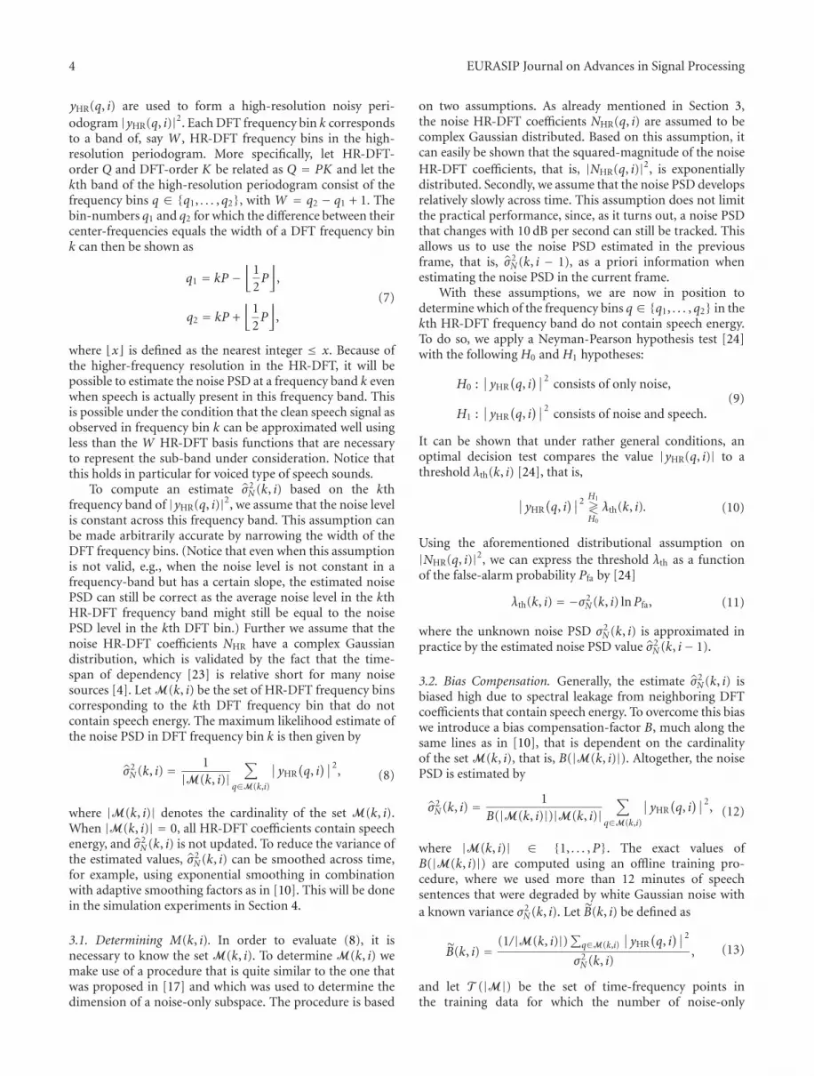
In this paper, we propose an alternative noise PSDtracking algorithm with approximately similar performanceas the method presented in [17], but with considerablyreduced computational complexity. The proposed methodis outlined in Figure 1. The method makes use of the factthat often speech sounds can be modelled using a small

EURASIP Journal on Advances in Signal Processing 3

number of complex exponentials [20]. Notice that this holdsin particular for voiced type of speech sounds, especiallyat lower frequencies. The noise PSD tracking method isbased on noisy periodograms computed using a DFT witha frequency resolution that is typically higher than that ofthe DFT used in the noise reduction algorithm itself. In thefollowing, we will use the expression HR-DFT to refer to thehigh-resolution DFT that is used to estimate the noise PSD.To refer to the DFT that is used to compute the noisy DFTcoefficients in the noise reduction algorithm we maintain theexpression DFT. For example, in the simulation experimentsreported in Section 4, we use a 256-points DFT and a 1024-points HR-DFT at a sampling rate of 8 kHz. Hence, due tothe difference in resolution between the DFT and the HR-DFT, every DFT bin corresponds to a sub-band of severalHR-DFT bins. The high-resolution periodogram is dividedin sub-bands, corresponding to the frequency bins obtainedby the DFT. Analogous to the method in [17] we divide theHR-DFT bins within each sub-band to contain noisy speechand noise only. The noise-only HR-DFT bins are used tocompute a maximum likelihood estimate of the noise PSDlevel.

The remainder of this paper is organized as follows. InSection 2 the basic notation and assumptions are introducedthat will be used throughout this paper. In Section 3 theproposed noise PSD estimation method based on high-resolution periodograms is presented. Furthermore, in Sec-tion 4 experimental results will be presented followed by adiscussion on the proposed noise PSD estimator in Section 5.Finally, in Section 6 concluding remarks are given.

2. DFT-Based Speech Estimators

Let the bandlimited and sampled time-domain noisy speechsignal be denoted by yt, where the subscript t explicitlyindicates that this is a time-domain signal. We assume thatyt consists of a clean speech signal xt that is degraded byadditive noise nt, that is,

yt = xt + nt . (1)

The noisy signal yt is divided in frames of length L1 byapplying a sliding window w1(m) with m ∈ {0, . . . ,L1 − 1}with a window-shift M. Let k and i be the frequency-binindex and time-frame index, respectively, and let K ≥ L1 bethe DFT order. The noisy DFT coefficients y(k, i) are thengiven by the discrete Fourier transform of the windowedtime-frames, that is,

y(k, i) =L1−1∑m=0

yt(iM + m)w1(m) exp

[−2πkmj

K

], (2)

where j =√−1 is the imaginary unit and where w1 is the

normalized analysis window such that∑L1−1

m=0 w21(m) = 1.

(This normalization is used to overcome energy differencesbetween the DFT and HR-DFT coefficients when usingdifferent analysis windows in both transforms.) Similarly,let x(k, i) and n(k, i) be the clean speech and noise DFT

coefficient at frequency bin k and time-frame i. Due tolinearity of the Fourier transform, it holds that

y(k, i) = x(k, i) + n(k, i). (3)

The DFT coefficients y(k, i), x(k, i), and n(k, i) are assumedto be realizations of the zero-mean complex-valued randomvariables Y(k, i), X(k, i), and N(k, i), respectively. Further, itis assumed that X(k, i) and N(k, i) are uncorrelated, that is,

E[X(k, i)N∗(k, i)] = 0 ∀k, i. (4)

In order to find an estimate of the clean speech DFTcoefficient x(k, i), say x(k, i), a gain function G(k, i) istypically applied to the noisy DFT coefficients, that is,

x(k, i) = G(k, i)y(k, i). (5)

There exist various ways to determine this gain function,for example, based on Bayesian principles [2–5] or basedon more heuristically motivated arguments, for example,spectral subtraction [21]. However, irrespective of how thegain function is derived, it holds that all gain functions are

dependent on the noise PSD σ2N (k, i) = E[|N(k, i)|2]. As

discussed above, this quantity is generally not known withcertainty, but must be estimated from the available data.

3. Noise PSD Estimation Based onHigh-Resolution Periodograms

In the proposed noise PSD tracking method we distinguishbetween two different type of time-frames. The time-framesthat are used for the actual processing of the noisy signal inthe noise reduction system have a length of L1 samples andare defined in Section 2. We refer to these time-frames assignal-frames. The second type will be called super-framesand have a length of L2 samples where generally L2 > L1.The super-frames are used to estimate the noise PSD usinghigh-resolution DFTs (HR-DFTs). Let D be the allowedalgorithmic delay in samples in addition to the delay of thesignal-frame. A super-frame with index i then comprises thetime samples yt(iM+m) withm ∈ {L1−L2+D, . . . ,L1−1+D}.For simplicity we assume that size and position of the super-frames with respect to the signal-frames is fixed. However,notice that size and position of the super-frames could bemade adaptive with respect to the underlying noisy signal, forexample, using a segmentation algorithm for noisy speech aspresented in [22].

Let Q ≥ L2 be the order of the HR-DFT and let w2 bea normalized window function such that

∑L2−1m=0 w

22(m) = 1.

The HR-DFT coefficient of a super-frame at frequency bin qand time-frame i is given by

yHR

(q, i)=

L1−1+D∑

m=L1−L2+D

yt(iM + m)w2(m) exp

[−2πqmj

Q

],

(6)

where the subscript HR indicates that this is a coefficientof the HR-DFT of a super-frame. The HR-DFT coefficients


yHR(q, i) are used to form a high-resolution noisy peri-

odogram |yHR(q, i)|2. Each DFT frequency bin k correspondsto a band of, say W , HR-DFT frequency bins in the high-resolution periodogram. More specifically, let HR-DFT-order Q and DFT-order K be related as Q = PK and let thekth band of the high-resolution periodogram consist of thefrequency bins q ∈ {q1, . . . , q2}, with W = q2 − q1 + 1. Thebin-numbers q1 and q2 for which the difference between theircenter-frequencies equals the width of a DFT frequency bink can then be shown as

q1 = kP −⌊

1

2P⌋

,

q2 = kP +

⌊1

2P⌋

,

(7)

where ⌊x⌋ is defined as the nearest integer ≤ x. Because ofthe higher-frequency resolution in the HR-DFT, it will bepossible to estimate the noise PSD at a frequency band k evenwhen speech is actually present in this frequency band. Thisis possible under the condition that the clean speech signal asobserved in frequency bin k can be approximated well usingless than the W HR-DFT basis functions that are necessaryto represent the sub-band under consideration. Notice thatthis holds in particular for voiced type of speech sounds.

To compute an estimate σ2N (k, i) based on the kth

frequency band of |yHR(q, i)|2, we assume that the noise levelis constant across this frequency band. This assumption canbe made arbitrarily accurate by narrowing the width of theDFT frequency bins. (Notice that even when this assumptionis not valid, e.g., when the noise level is not constant in afrequency-band but has a certain slope, the estimated noisePSD can still be correct as the average noise level in the kthHR-DFT frequency band might still be equal to the noisePSD level in the kth DFT bin.) Further we assume that thenoise HR-DFT coefficients NHR have a complex Gaussiandistribution, which is validated by the fact that the time-span of dependency [23] is relative short for many noisesources [4]. Let M(k, i) be the set of HR-DFT frequency binscorresponding to the kth DFT frequency bin that do notcontain speech energy. The maximum likelihood estimate ofthe noise PSD in DFT frequency bin k is then given by

σ2N (k, i) = 1

|M(k, i)|∑

q∈M(k,i)

∣∣yHR

(q, i)∣∣2

, (8)

where |M(k, i)| denotes the cardinality of the set M(k, i).When |M(k, i)| = 0, all HR-DFT coefficients contain speechenergy, and σ2

N (k, i) is not updated. To reduce the variance ofthe estimated values, σ2

N (k, i) can be smoothed across time,for example, using exponential smoothing in combinationwith adaptive smoothing factors as in [10]. This will be donein the simulation experiments in Section 4.

3.1. Determining M(k, i). In order to evaluate (8), it isnecessary to know the set M(k, i). To determine M(k, i) wemake use of a procedure that is quite similar to the one thatwas proposed in [17] and which was used to determine thedimension of a noise-only subspace. The procedure is based

on two assumptions. As already mentioned in Section 3,the noise HR-DFT coefficients NHR(q, i) are assumed to becomplex Gaussian distributed. Based on this assumption, itcan easily be shown that the squared-magnitude of the noise

HR-DFT coefficients, that is, |NHR(q, i)|2, is exponentiallydistributed. Secondly, we assume that the noise PSD developsrelatively slowly across time. This assumption does not limitthe practical performance, since, as it turns out, a noise PSDthat changes with 10 dB per second can still be tracked. Thisallows us to use the noise PSD estimated in the previousframe, that is, σ2

N (k, i − 1), as a priori information whenestimating the noise PSD in the current frame.

With these assumptions, we are now in position todetermine which of the frequency bins q ∈ {q1, . . . , q2} in thekth HR-DFT frequency band do not contain speech energy.To do so, we apply a Neyman-Pearson hypothesis test [24]with the following H0 and H1 hypotheses:

H0 :∣∣yHR

(q, i)∣∣2

consists of only noise,

H1 :∣∣yHR

(q, i)∣∣2

consists of noise and speech.(9)

It can be shown that under rather general conditions, anoptimal decision test compares the value |yHR(q, i)| to athreshold λth(k, i) [24], that is,

∣∣yHR

(q, i)∣∣2

H1

≷H0

λth(k, i). (10)

Using the aforementioned distributional assumption on

|NHR(q, i)|2, we can express the threshold λth as a functionof the false-alarm probability Pfa by [24]

λth(k, i) = −σ2N (k, i) lnPfa, (11)

where the unknown noise PSD σ2N (k, i) is approximated in

practice by the estimated noise PSD value σ2N (k, i− 1).

3.2. Bias Compensation. Generally, the estimate σ2N (k, i) is

biased high due to spectral leakage from neighboring DFTcoefficients that contain speech energy. To overcome this biaswe introduce a bias compensation-factor B, much along thesame lines as in [10], that is dependent on the cardinalityof the set M(k, i), that is, B(|M(k, i)|). Altogether, the noisePSD is estimated by

σ2N (k, i) = 1

B(|M(k, i)|)|M(k, i)|∑

q∈M(k,i)

∣∣yHR

(q, i)∣∣2

, (12)

where |M(k, i)| ∈ {1, . . . ,P}. The exact values ofB(|M(k, i)|) are computed using an offline training pro-cedure, where we used more than 12 minutes of speechsentences that were degraded by white Gaussian noise with

a known variance σ2N (k, i). Let B(k, i) be defined as

B(k, i) =(1/|M(k, i)|)

∑q∈M(k,i)

∣∣yHR

(q, i)∣∣2

σ2N (k, i)

, (13)

and let T (|M|) be the set of time-frequency points inthe training data for which the number of noise-only


bins in a frequency band is estimated to be |M|. Thebias compensation-factor B(|M(k, i)|), is then computed by

averaging B(k, i) over the set T (|M|) leading to

B(|M|) = 1

|T (|M|)|∑

(k,i)∈T (|M|)B(k, i). (14)

Although this training procedure makes use of white noisein order to compute B(|M|), this does not limit theapplicability of the proposed noise PSD estimator as it can beused to track both white and non-white noise sources as longas the noise-level in a band can be assumed approximatelyconstant. The training procedure is applied using only oneSNR, that is, at a global SNR of 10 dB. Clearly, the biascompensation could be extended by making B(|M|) alsoa function of SNR. However, in the results presented inSection 4 we keep B(|M|) independent of SNR in order tokeep complexity and storage requirements low.

3.3. Algorithm Overview. In this section, we give a summaryof the necessary processing steps in the proposed algorithm.It is assumed that all processing steps are repeated for eachtime-frame index i. However, when less processing power isavailable the update rate could be reduced.

(1) Compute HR-DFT of a windowed noisy super-frameusing (6).

(2) Determine the set |M(k, i)| for each band k using (9).

(3) Compute σ2N (k, i) for each band k using (12).

(4) Apply smoothing across time of the estimate noisePSD in order to reduce its variance.

Whenever |M(k, i)| = 0, all frequency bins in the bandcontain speech energy in which case it is not possible toupdate the noise PSD in that band during time-frame i.In these situations, the estimate from the time-frame i − 1is used. To overcome a complete locking of the noise PSDestimator under extreme situations when |M(k, i)| = 0 for avery long time we adopt the safety-net proposed in [13] and

compute the minimum Pmin(k, i) of |y(k, i)|2 across a longtime-interval, for example, a time-interval of one second.Using Pmin(k, i), the noise PSD is updated by

σ ′2

N (k, i) = max[σ2N (k, i),Pmin(k, i)

]. (15)

4. Experimental Results

For performance evaluation of the proposed method fornoise PSD estimation we compare its performance withthree reference methods, namely, noise PSD estimation basedon MS as proposed in [10], QB noise PSD estimation asproposed in [12] with quantile parameter p = 0.5 anda buffer length of 20 frames, and noise PSD estimationbased on the DFT-subspace approach as proposed in [17].The speech database that we used consists of more than 7minutes of Danish speech that was read from newspapersby 17 different speakers, 9 female speakers and 8 malespeakers, and does not contain long portions of silence.

These speech signals were not used for computation of thebias compensation in Section 3.2. The speech signals weredegraded by a variety of noise sources at input SNRs of 0,5, 10, and 15 dB. Both the speech and the noise signals wereused at a sampling frequency of 8 kHz. All signals start with anoise-only period of 0.5 seconds. All algorithms use the first0.1 seconds for initialization; these noise-only samples areexcluded from all performance measurements. The length ofthe signal-frames is set to L1 = 256, that is, 32 milliseconds.The length L2 of the super-frames for the proposed methodis a tradeoff between complexity constraints and stationarityrequirements on the noisy speech signal on one hand, andthe potential to exploit the increased frequency resolutionfor noise PSD estimation on the other hand. In Section 4.1.2experiments will be performed that also reflect this tradeoff.Based on these experiments it follows that the best choicein terms of noise tracking performance for the length ofthe super-frames is around 70–100 milliseconds. In orderto make a fair comparison possible with the DFT-subspaceapproach [17], we therefore chose the length L2 such that itequals the amount of data used in [17] and use L2 = 640samples, that is, 80 milliseconds.

The signal-frames have an overlap of 50% and arewindowed using a square-root-Hann window. The super-frames are windowed using a Hann window. The order ofthe DFT and the HR-DFT are K = 256 and Q = 1024,respectively, and are chosen as an integer power of 2 tofacilitate an efficient implementation of the DFT using FFTs.The false-alarm probability in (11) was set to Pfa = 0.001.The estimated values of B(|M|) are between 1 and 3.7.Obviously, the estimated bias compensation factors B(|M|)depend on the chosen parameter settings, for example,super-frame length L2 and the HR-DFT order Q. In theexperimental results presented in this section we focus onreal-time applications that require low algorithmic delay.Therefore, we set the allowed algorithmic delay to D = 0 forall methods. Further, we apply the same safety-net procedureas in (15) to the DFT-subspace approach [17] to avoidlocking of the estimator.

4.1. Noise PSD Estimation Performance. Because optimalestimators used for noise reduction are always functionsof the true noise variance σ2

N (k, i), we can evaluate theperformance of noise PSD tracking algorithms by measuringdirectly the error between σ2

N (k, i) and its estimate σ2N (k, i).

For this purpose we use the symmetric log-error distortionmeasure defined in [17] as

LogErr = 1

IK

K∑

k=1

I∑

i=1

∣∣∣∣∣10 log

[σ2N (k, i)

σ2N (k, i)

]∣∣∣∣∣ (dB), (16)

where I denotes the total number of signal-frames andσ2N (k, i) denotes the ideal noise PSD that is obtained by

smoothing measured noise periodograms across time usingan exponential window, that is,

σ2N (k, i) = ασ2

N (k, i− 1) + (1− α)|n(k, i)|2, (17)

with a smoothing factor α = 0.9 [10].


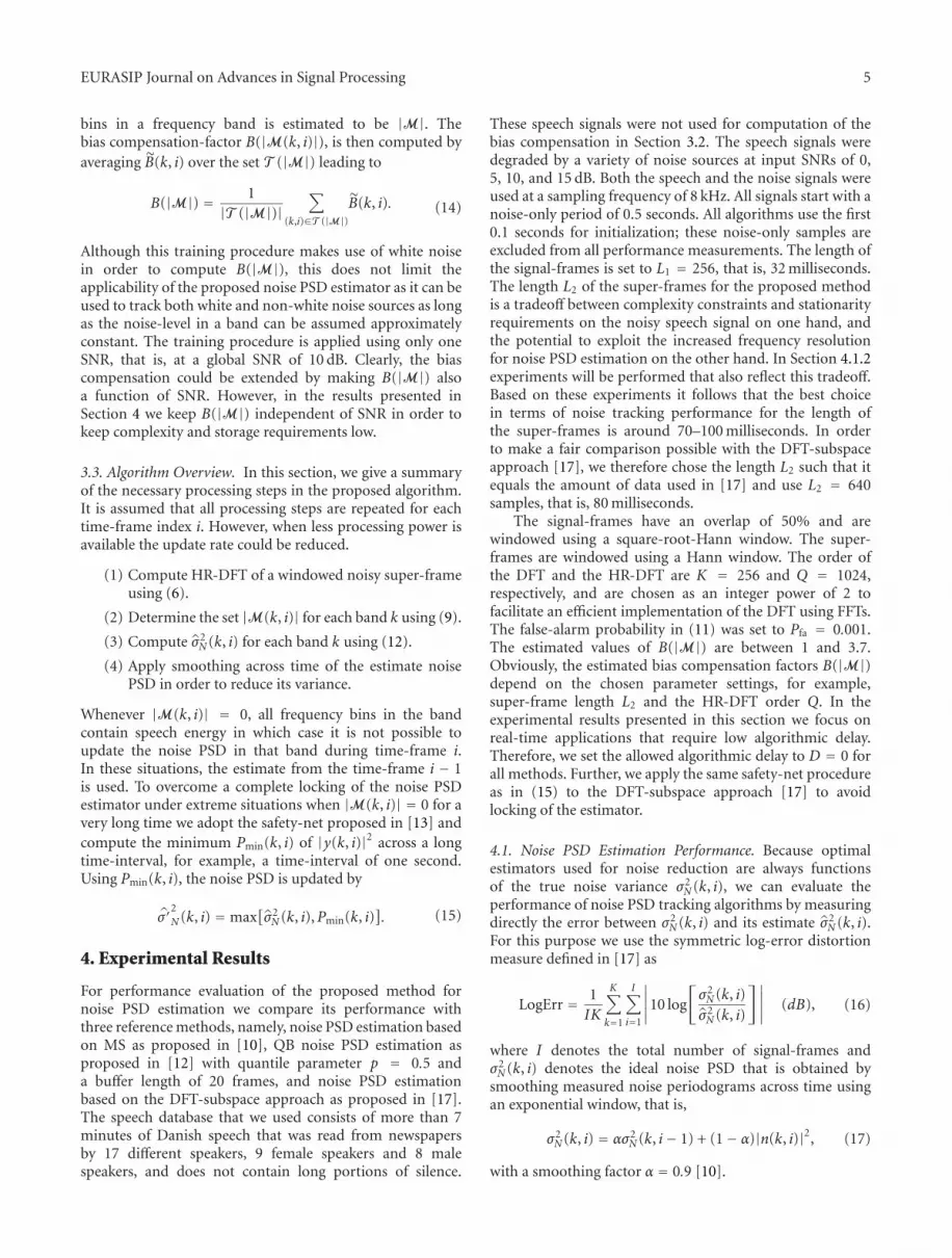
4.1.1. Synthetic Performance Example. To demonstrate thepotential of the proposed approach, we consider a syntheticexample of noise PSD estimation where the presence ofspeech is modelled by a sinusoid at a frequency of 937.5 Hz,that is, centered in the 31st frequency bin. This cleansynthetic signal is shown in Figure 2(a). During the timeinstance of approximately 2 till 5 seconds, the sinusoid iscontinuously present in periods of 450 milliseconds, eachtime followed by a 150 ms period where the sinusoid isabsent in order to model speech absence. Subsequently,this synthetic clean signal is degraded by white Gaussiannoise. The SNR in the frequency bin under considerationis approximately 36 dB during presence of the sinusoidalcomponent in the first 3.5 seconds. In the time spanfrom 3.5 till 4.5 seconds the SNR decreases from 36 dBto 30 dB. For visibility the results are distributed over twosubplots. Figure 2(b) shows the noise PSD estimated by theproposed method and MS, compared to the true noise PSD.Figure 2(c) shows the noise PSD estimated by the DFT-subspace approach and QB noise PSD estimation, comparedto the true noise PSD.

From the comparison in Figures 2(b) and 2(c) it is clearthat both the MS and the QB approach heavily overestimatethe noise PSD. This is caused by the presence of the sinusoidalcomponent, which leads to tracking of the PSD of the noisysinusoid instead of the noise PSD. The proposed approachand the DFT-subspace approach show accurate tracking ofthe changing noise level. That the proposed approach isable to track the changing noise level is due to the higherfrequency resolution that is exploited. This also becomesclear from Figure 2(d) where the number of HR-DFT bins isshown for the DFT bin under consideration that are classifiedas noise-only, that is, |M(k, i)|. As expected, when thereis no speech presence |M(k, i)| equals the total numberof HR-DFT bins that fall within one DFT bin, that is,under the given parameter settings |M(k, i)| = 5. Whenthe sinusoidal component is present, |M(k, i)| decreases toone or two, which means that the estimated noise PSD canstill be updated even though the sinusoidal component ispresent.

4.1.2. Super-Frame Size L2. In this section, we investigatethe relation between the length of the super-frames L2 andnoise tracking performance. To do so, we degraded thespeech signals in the database by two different noise sources,namely, white noise and non-stationary white noise. Thenon-stationary white noise consists of white noise that ismodulated by the following function:

f (m) = 1 + 0.5 sin

(2πm f mod

fs

), (18)

where m is the sample index, fs the sampling frequency,and f mod the modulation frequency, which increases linearlyin 25 seconds from 0 Hz to 0.5 Hz, that is, a maximumchange of the noise PSD of approximately 10 dB per second.An example of such a modulated white noise sequencecan be seen in Figure 6. Subsequently, the proposed noisetracking algorithm is applied with several super-frame sizes

−1

0

1

0 1 2 3 4 5 6 7 8

Time (s)

(a)

203040

σ2 N

(dB

)

0 1 2 3 4 5 6 7 8

Time (s)

(b)

203040

σ2 N

(dB

)

0 1 2 3 4 5 6 7 8

Time (s)

(c)

135

|M(k

,i)|

0 1 2 3 4 5 6 7 8

Time (s)

(d)

Figure 2: Synthetic noise tracking example. (a) Clean syntheticsignal. (b) Comparison between true noise PSD (dotted line),proposed approach (solid line), and MS (dashed line) for DFTbin centered around 937.5 Hz. (c) Comparison between true noisePSD (dotted line), DFT-subspace approach (solid line), and QBapproach (dashed line) for DFT bin centered around 937.5 Hz. (d)Cardinality of the set M(k, i) for the frequency bin centered around937.5 Hz.

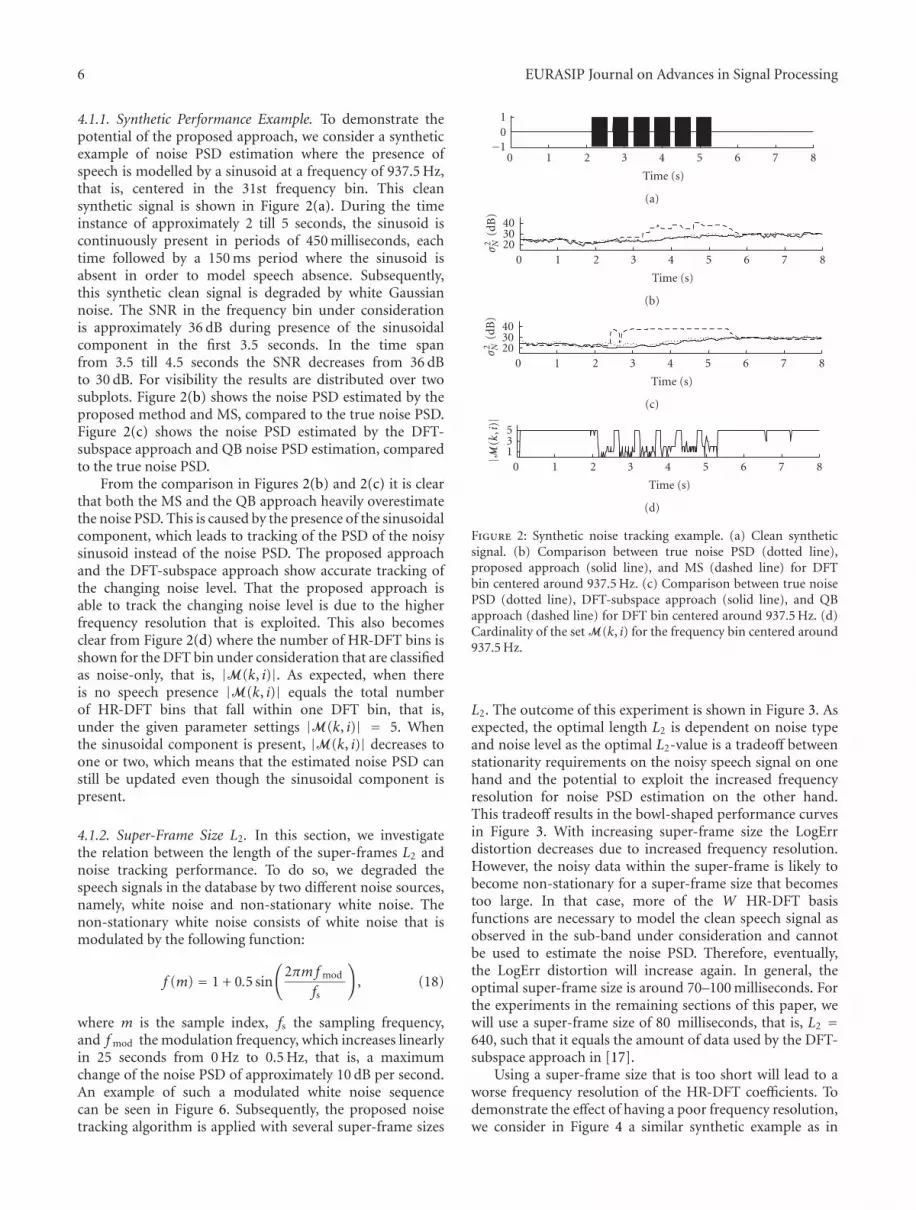
L2. The outcome of this experiment is shown in Figure 3. Asexpected, the optimal length L2 is dependent on noise typeand noise level as the optimal L2-value is a tradeoff betweenstationarity requirements on the noisy speech signal on onehand and the potential to exploit the increased frequencyresolution for noise PSD estimation on the other hand.This tradeoff results in the bowl-shaped performance curvesin Figure 3. With increasing super-frame size the LogErrdistortion decreases due to increased frequency resolution.However, the noisy data within the super-frame is likely tobecome non-stationary for a super-frame size that becomestoo large. In that case, more of the W HR-DFT basisfunctions are necessary to model the clean speech signal asobserved in the sub-band under consideration and cannotbe used to estimate the noise PSD. Therefore, eventually,the LogErr distortion will increase again. In general, theoptimal super-frame size is around 70–100 milliseconds. Forthe experiments in the remaining sections of this paper, wewill use a super-frame size of 80 milliseconds, that is, L2 =640, such that it equals the amount of data used by the DFT-subspace approach in [17].

Using a super-frame size that is too short will lead to aworse frequency resolution of the HR-DFT coefficients. Todemonstrate the effect of having a poor frequency resolution,we consider in Figure 4 a similar synthetic example as in


0.8

1

1.2

1.4

40 60 80 100 120

Super-frame size (ms)

Lo

gErr

(dB

)

(a)

0.8

1

1.2

1.4

40 60 80 100 120


Lo

gErr

(dB

)

(b)

0.9

1

1.1

1.2

1.3

40 60 80 100 120


Lo

gErr

(dB

)

(c)

1.1

1.2

1.3

1.4

1.5

40 60 80 100 120


Lo

gErr

(dB

)

(d)

Figure 3: Noise tracking performance in terms of LogErr (dB) as a function of the length of the super-frames for stationary Gaussian whitenoise (solid line) and nonstationary Gaussian white noise (dashed line) at an input SNR of (a) 0 dB (b) 5 dB (c) 10 dB (d) 15 dB.

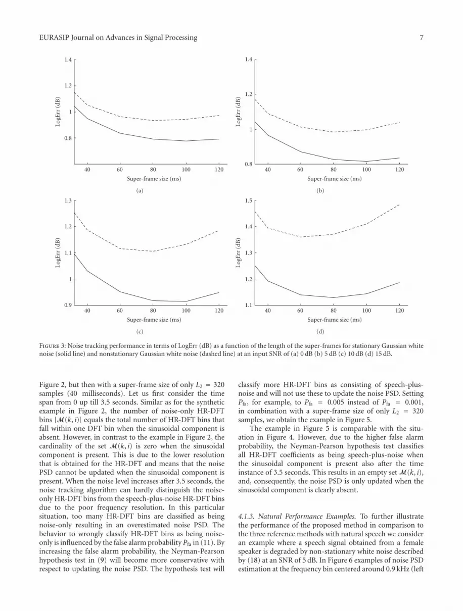
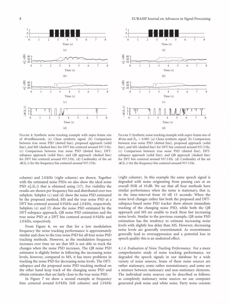
Figure 2, but then with a super-frame size of only L2 = 320samples (40 milliseconds). Let us first consider the timespan from 0 up till 3.5 seconds. Similar as for the syntheticexample in Figure 2, the number of noise-only HR-DFTbins |M(k, i)| equals the total number of HR-DFT bins thatfall within one DFT bin when the sinusoidal component isabsent. However, in contrast to the example in Figure 2, thecardinality of the set M(k, i) is zero when the sinusoidalcomponent is present. This is due to the lower resolutionthat is obtained for the HR-DFT and means that the noisePSD cannot be updated when the sinusoidal component ispresent. When the noise level increases after 3.5 seconds, thenoise tracking algorithm can hardly distinguish the noise-only HR-DFT bins from the speech-plus-noise HR-DFT binsdue to the poor frequency resolution. In this particularsituation, too many HR-DFT bins are classified as beingnoise-only resulting in an overestimated noise PSD. Thebehavior to wrongly classify HR-DFT bins as being noise-only is influenced by the false alarm probability Pfa in (11). Byincreasing the false alarm probability, the Neyman-Pearsonhypothesis test in (9) will become more conservative withrespect to updating the noise PSD. The hypothesis test will

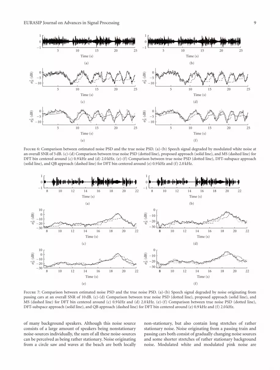
classify more HR-DFT bins as consisting of speech-plus-noise and will not use these to update the noise PSD. SettingPfa, for example, to Pfa = 0.005 instead of Pfa = 0.001,in combination with a super-frame size of only L2 = 320samples, we obtain the example in Figure 5.

The example in Figure 5 is comparable with the situ-ation in Figure 4. However, due to the higher false alarmprobability, the Neyman-Pearson hypothesis test classifiesall HR-DFT coefficients as being speech-plus-noise whenthe sinusoidal component is present also after the timeinstance of 3.5 seconds. This results in an empty set M(k, i),and, consequently, the noise PSD is only updated when thesinusoidal component is clearly absent.

4.1.3. Natural Performance Examples. To further illustratethe performance of the proposed method in comparison tothe three reference methods with natural speech we consideran example where a speech signal obtained from a femalespeaker is degraded by non-stationary white noise describedby (18) at an SNR of 5 dB. In Figure 6 examples of noise PSDestimation at the frequency bin centered around 0.9 kHz (left


−1

0

1

0 1 2 3 4 5 6 7 8

Time (s)

(a)

203040

σ2 N

(dB

)

0 1 2 3 4 5 6 7 8

Time (s)

(b)

203040

σ2 N

(dB

)

0 1 2 3 4 5 6 7 8

Time (s)

(c)

135

|M(k

,i)|

0 1 2 3 4 5 6 7 8

Time (s)

(d)

Figure 4: Synthetic noise tracking example with super-frame sizeof 40 milliseconds. (a) Clean synthetic signal. (b) Comparisonbetween true noise PSD (dotted line), proposed approach (solidline), and MS (dashed line) for DFT bin centered around 937.5 Hz.(c) Comparison between true noise PSD (dotted line), DFT-subspace approach (solid line), and QB approach (dashed line)for DFT bin centered around 937.5 Hz. (d) Cardinality of the setM(k, i) for the frequency bin centered around 937.5 Hz.

column) and 2.0 kHz (right column) are shown. Togetherwith the estimated noise PSDs we also show the ideal noisePSD σ2

N (k, i) that is obtained using (17). For visibility theresults are shown per frequency bin and distributed over twosubplots. Subplot (c) and (d) show the noise PSD estimatedby the proposed method, MS and the true noise PSD at aDFT bin centered around 0.9 kHz and 2.0 kHz, respectively.Subplots (e) and (f) show the noise PSD estimated by theDFT-subspace approach, QB noise PSD estimation and thetrue noise PSD at a DFT bin centered around 0.9 kHz and2.0 kHz, respectively.

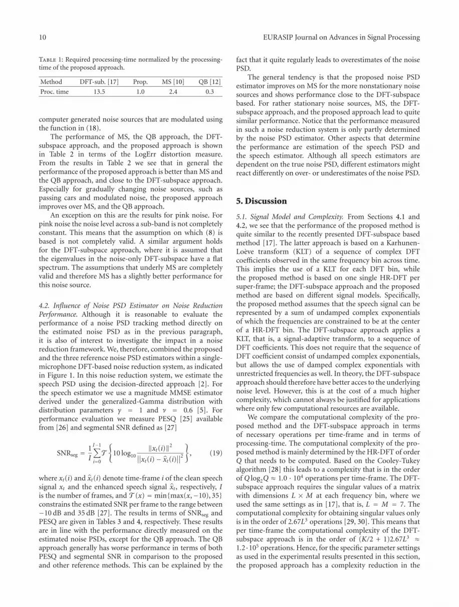
From Figure 6, we see that for a low modulationfrequency the noise tracking performance is approximatelysimilar and close to the true noise PSD for all four noise PSDtracking methods. However, as the modulation frequencyincreases over time we see that MS is not able to track thechanges when the noise PSD increases. The QB noise PSDestimator is slightly better in following the increasing noiselevels, however, compared to MS, it has more problems intracking the noise PSD for decreasing noise levels. The DFT-subspace and the proposed noise PSD tracking method onthe other hand keep track of the changing noise PSD andobtain estimates that are fairly close to the true noise PSD.

In Figure 7 we show a second example at frequencybins centered around 0.9 kHz (left column) and 2.0 kHz

−1

0

1

0 1 2 3 4 5 6 7 8

Time (s)

(a)

203040

σ2 N

(dB

)

0 1 2 3 4 5 6 7 8

Time (s)

(b)

203040

σ2 N

(dB

)

0 1 2 3 4 5 6 7 8

Time (s)

(c)

135

|M(k

,i)|

0 1 2 3 4 5 6 7 8

Time (s)

(d)

Figure 5: Synthetic noise tracking example with super-frame size of40 ms and Pfa = 0.005. (a) Clean synthetic signal. (b) Comparisonbetween true noise PSD (dotted line), proposed approach (solidline), and MS (dashed line) for DFT bin centered around 937.5 Hz.(c) Comparison between true noise PSD (dotted line), DFT-subspace approach (solid line), and QB approach (dashed line)for DFT bin centered around 937.5 Hz. (d) Cardinality of the setM(k, i) for the frequency bin centered around 937.5 Hz.

(right column). In this example the same speech signal isdegraded with noise originating from passing cars at anoverall SNR of 10 dB. We see that all four methods havesimilar performance when the noise is stationary, that is,in the time-interval from 10 till 15 seconds. When thenoise level changes rather fast both the proposed and DFT-subspace-based noise PSD tracker show almost immediatetracking of the changing noise PSD, while both the QBapproach and MS are unable to track these fast increasingnoise levels. Similar to the previous example, QB noise PSDestimation has the tendency to estimate increasing noiselevels with slightly less delay than MS. However, decreasingnoise levels are generally overestimated. As overestimatesgenerally lead to oversuppression and a potential loss inspeech quality this is an undesired effect.

4.1.4. Evaluation of Noise Tracking Performance. For a morecomprehensive study of noise tracking performance, wedegraded the speech signals in our database by a widevariety of noise sources. Some of these noise sources arerather stationary, some rather nonstationary, and some area mixture between stationary and non-stationary elements.The individual noise sources can be described as follows:as completely stationary noise sources we use computergenerated pink noise and white noise. Party noise consists


−1

0

1

5 10 15 20 25

Time (s)

(a)

−1

0

1

5 10 15 20 25

Time (s)

(b)

−10

−5

0

5 10 15 20

σ2 N

(dB

)

25

Time (s)

(c)

−10

−5

0

5 10 15 20

σ2 N

(dB

)

25

Time (s)

(d)

−10

−5

0

5 10 15 20

σ2 N

(dB

)

25

Time (s)

(e)

−10

−5

0

5 10 15 20

σ2 N

(dB

)

25

Time (s)

(f)

Figure 6: Comparison between estimated noise PSD and the true noise PSD. (a)-(b) Speech signal degraded by modulated white noise atan overall SNR of 5 dB. (c)-(d) Comparison between true noise PSD (dotted line), proposed approach (solid line), and MS (dashed line) forDFT bin centered around (c) 0.9 kHz and (d) 2.0 kHz. (e)-(f) Comparison between true noise PSD (dotted line), DFT-subspace approach(solid line), and QB approach (dashed line) for DFT bin centered around (e) 0.9 kHz and (f) 2.0 kHz.

−1

0

1

8 10 12 14 16 18 20 22

Time (s)

(a)

−1

0

1

8 10 12 14 16 18 20 22

Time (s)

(b)

−30−20−10

0

10

8 10

σ2 N

(dB

)

12 14 16 18 20 22

Time (s)

(c)

−30

−20

−10

σ2 N

(dB

)

0

88 10 12 14 16 18 20 22

Time (s)

(d)

−30−20−10

0

10

8 10

σ2 N

(dB

)

12 14 16 18 20 22

Time (s)

(e)

−30

−20

−10

σ2 N

(dB

)

0

88 10 12 14 16 18 20 22

Time (s)

(f)

Figure 7: Comparison between estimated noise PSD and the true noise PSD. (a)-(b) Speech signal degraded by noise originating frompassing cars at an overall SNR of 10 dB. (c)-(d) Comparison between true noise PSD (dotted line), proposed approach (solid line), andMS (dashed line) for DFT bin centered around (c) 0.9 kHz and (d) 2.0 kHz. (e)-(f) Comparison between true noise PSD (dotted line),DFT-subspace approach (solid line), and QB approach (dashed line) for DFT bin centered around (e) 0.9 kHz and (f) 2.0 kHz.

of many background speakers. Although this noise sourceconsists of a large amount of speakers being nonstationarynoise-sources individually, the sum of all these noise-sourcescan be perceived as being rather stationary. Noise originatingfrom a circle saw and waves at the beach are both locally

non-stationary, but also contain long stretches of ratherstationary noise. Noise originating from a passing train andpassing cars both consist of gradually changing noise sourcesand some shorter stretches of rather stationary backgroundnoise. Modulated white and modulated pink noise are


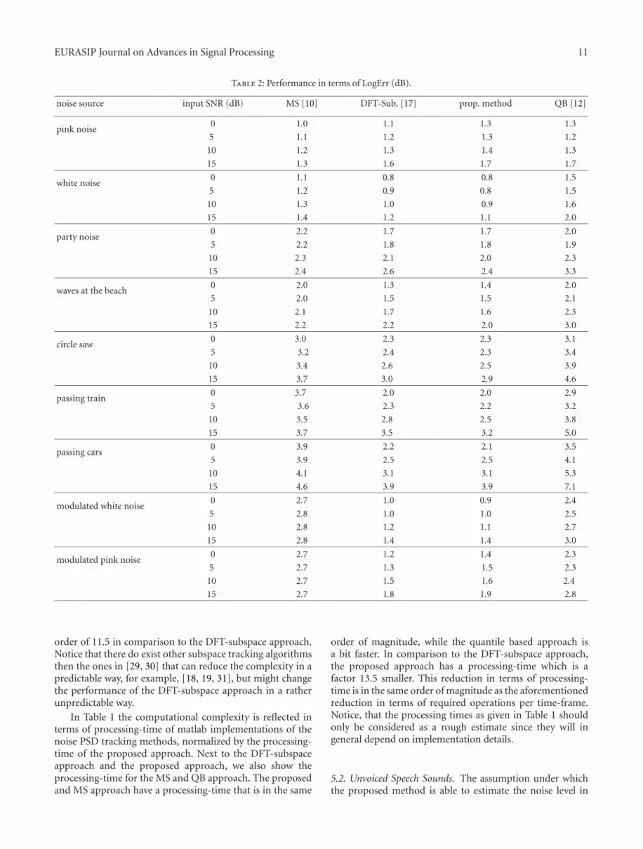
Table 1: Required processing-time normalized by the processing-time of the proposed approach.

Method DFT-sub. [17] Prop. MS [10] QB [12]

Proc. time 13.5 1.0 2.4 0.3

computer generated noise sources that are modulated usingthe function in (18).

The performance of MS, the QB approach, the DFT-subspace approach, and the proposed approach is shownin Table 2 in terms of the LogErr distortion measure.From the results in Table 2 we see that in general theperformance of the proposed approach is better than MS andthe QB approach, and close to the DFT-subspace approach.Especially for gradually changing noise sources, such aspassing cars and modulated noise, the proposed approachimproves over MS, and the QB approach.

An exception on this are the results for pink noise. Forpink noise the noise level across a sub-band is not completelyconstant. This means that the assumption on which (8) isbased is not completely valid. A similar argument holdsfor the DFT-subspace approach, where it is assumed thatthe eigenvalues in the noise-only DFT-subspace have a flatspectrum. The assumptions that underly MS are completelyvalid and therefore MS has a slightly better performance forthis noise source.

4.2. Influence of Noise PSD Estimator on Noise ReductionPerformance. Although it is reasonable to evaluate theperformance of a noise PSD tracking method directly onthe estimated noise PSD as in the previous paragraph,it is also of interest to investigate the impact in a noisereduction framework. We, therefore, combined the proposedand the three reference noise PSD estimators within a single-microphone DFT-based noise reduction system, as indicatedin Figure 1. In this noise reduction system, we estimate thespeech PSD using the decision-directed approach [2]. Forthe speech estimator we use a magnitude MMSE estimatorderived under the generalized-Gamma distribution withdistribution parameters γ = 1 and ν = 0.6 [5]. Forperformance evaluation we measure PESQ [25] availablefrom [26] and segmental SNR defined as [27]

SNRseg =1

I

I−1∑

i=0

T

{10 log10

‖xt(i)‖2

∥∥xt(i)− xt(i)∥∥2

}, (19)

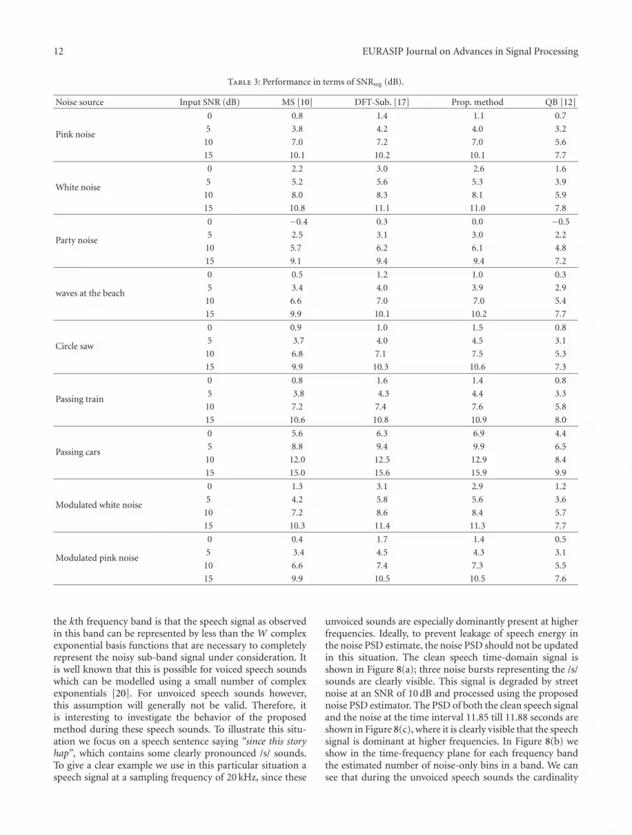
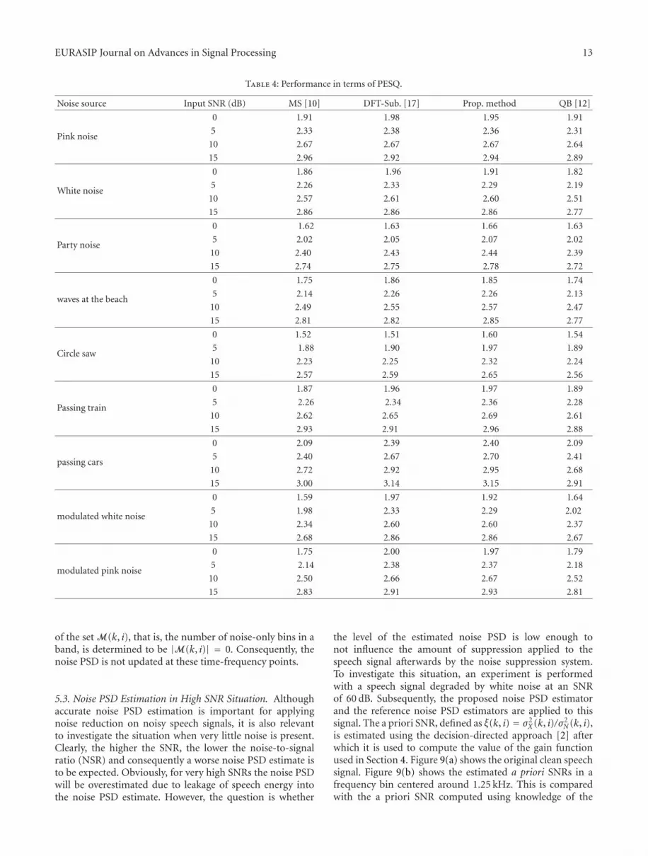
where xt(i) and xt(i) denote time-frame i of the clean speechsignal xt and the enhanced speech signal xt, respectively, Iis the number of frames, and T (x) = min{max(x,−10), 35}constrains the estimated SNR per frame to the range between−10 dB and 35 dB [27]. The results in terms of SNRseg andPESQ are given in Tables 3 and 4, respectively. These resultsare in line with the performance directly measured on theestimated noise PSDs, except for the QB approach. The QBapproach generally has worse performance in terms of bothPESQ and segmental SNR in comparison to the proposedand other reference methods. This can be explained by the

fact that it quite regularly leads to overestimates of the noisePSD.

The general tendency is that the proposed noise PSDestimator improves on MS for the more nonstationary noisesources and shows performance close to the DFT-subspacebased. For rather stationary noise sources, MS, the DFT-subspace approach, and the proposed approach lead to quitesimilar performance. Notice that the performance measuredin such a noise reduction system is only partly determinedby the noise PSD estimator. Other aspects that determinethe performance are estimation of the speech PSD andthe speech estimator. Although all speech estimators aredependent on the true noise PSD, different estimators mightreact differently on over- or underestimates of the noise PSD.

5. Discussion

5.1. Signal Model and Complexity. From Sections 4.1 and4.2, we see that the performance of the proposed method isquite similar to the recently presented DFT-subspace basedmethod [17]. The latter approach is based on a Karhunen-Loeve transform (KLT) of a sequence of complex DFTcoefficients observed in the same frequency bin across time.This implies the use of a KLT for each DFT bin, whilethe proposed method is based on one single HR-DFT persuper-frame; the DFT-subspace approach and the proposedmethod are based on different signal models. Specifically,the proposed method assumes that the speech signal can berepresented by a sum of undamped complex exponentialsof which the frequencies are constrained to be at the centerof a HR-DFT bin. The DFT-subspace approach applies aKLT, that is, a signal-adaptive transform, to a sequence ofDFT coefficients. This does not require that the sequence ofDFT coefficient consist of undamped complex exponentials,but allows the use of damped complex exponentials withunrestricted frequencies as well. In theory, the DFT-subspaceapproach should therefore have better acces to the underlyingnoise level. However, this is at the cost of a much highercomplexity, which cannot always be justified for applicationswhere only few computational resources are available.

We compare the computational complexity of the pro-posed method and the DFT-subspace approach in termsof necessary operations per time-frame and in terms ofprocessing-time. The computational complexity of the pro-posed method is mainly determined by the HR-DFT of orderQ that needs to be computed. Based on the Cooley-Tukeyalgorithm [28] this leads to a complexity that is in the orderof Q log2Q ≈ 1.0 · 104 operations per time-frame. The DFT-subspace approach requires the singular values of a matrixwith dimensions L × M at each frequency bin, where weused the same settings as in [17], that is, L = M = 7. Thecomputational complexity for obtaining singular values onlyis in the order of 2.67L3 operations [29, 30]. This means thatper time-frame the computational complexity of the DFT-subspace approach is in the order of (K/2 + 1)2.67L3 ≈1.2·105 operations. Hence, for the specific parameter settingsas used in the experimental results presented in this section,the proposed approach has a complexity reduction in the


Table 2: Performance in terms of LogErr (dB).

noise source input SNR (dB) MS [10] DFT-Sub. [17] prop. method QB [12]

pink noise0 1.0 1.1 1.3 1.3

5 1.1 1.2 1.3 1.2

10 1.2 1.3 1.4 1.3

15 1.3 1.6 1.7 1.7

white noise0 1.1 0.8 0.8 1.5

5 1.2 0.9 0.8 1.5

10 1.3 1.0 0.9 1.6

15 1.4 1.2 1.1 2.0

party noise0 2.2 1.7 1.7 2.0

5 2.2 1.8 1.8 1.9

10 2.3 2.1 2.0 2.3

15 2.4 2.6 2.4 3.3

waves at the beach0 2.0 1.3 1.4 2.0

5 2.0 1.5 1.5 2.1

10 2.1 1.7 1.6 2.3

15 2.2 2.2 2.0 3.0

circle saw0 3.0 2.3 2.3 3.1

5 3.2 2.4 2.3 3.4

10 3.4 2.6 2.5 3.9

15 3.7 3.0 2.9 4.6

passing train0 3.7 2.0 2.0 2.9

5 3.6 2.3 2.2 3.2

10 3.5 2.8 2.5 3.8

15 3.7 3.5 3.2 5.0

passing cars0 3.9 2.2 2.1 3.5

5 3.9 2.5 2.5 4.1

10 4.1 3.1 3.1 5.3

15 4.6 3.9 3.9 7.1

modulated white noise0 2.7 1.0 0.9 2.4

5 2.8 1.0 1.0 2.5

10 2.8 1.2 1.1 2.7

15 2.8 1.4 1.4 3.0

modulated pink noise0 2.7 1.2 1.4 2.3

5 2.7 1.3 1.5 2.3

10 2.7 1.5 1.6 2.4

15 2.7 1.8 1.9 2.8

order of 11.5 in comparison to the DFT-subspace approach.Notice that there do exist other subspace tracking algorithmsthen the ones in [29, 30] that can reduce the complexity in apredictable way, for example, [18, 19, 31], but might changethe performance of the DFT-subspace approach in a ratherunpredictable way.

In Table 1 the computational complexity is reflected interms of processing-time of matlab implementations of thenoise PSD tracking methods, normalized by the processing-time of the proposed approach. Next to the DFT-subspaceapproach and the proposed approach, we also show theprocessing-time for the MS and QB approach. The proposedand MS approach have a processing-time that is in the same

order of magnitude, while the quantile based approach isa bit faster. In comparison to the DFT-subspace approach,the proposed approach has a processing-time which is afactor 13.5 smaller. This reduction in terms of processing-time is in the same order of magnitude as the aforementionedreduction in terms of required operations per time-frame.Notice, that the processing times as given in Table 1 shouldonly be considered as a rough estimate since they will ingeneral depend on implementation details.

5.2. Unvoiced Speech Sounds. The assumption under whichthe proposed method is able to estimate the noise level in


Table 3: Performance in terms of SNRseg (dB).

Noise source Input SNR (dB) MS [10] DFT-Sub. [17] Prop. method QB [12]

Pink noise

0 0.8 1.4 1.1 0.7

5 3.8 4.2 4.0 3.2

10 7.0 7.2 7.0 5.6

15 10.1 10.2 10.1 7.7

White noise

0 2.2 3.0 2.6 1.6

5 5.2 5.6 5.3 3.9

10 8.0 8.3 8.1 5.9

15 10.8 11.1 11.0 7.8

Party noise

0 −0.4 0.3 0.0 −0.5

5 2.5 3.1 3.0 2.2

10 5.7 6.2 6.1 4.8

15 9.1 9.4 9.4 7.2

waves at the beach

0 0.5 1.2 1.0 0.3

5 3.4 4.0 3.9 2.9

10 6.6 7.0 7.0 5.4

15 9.9 10.1 10.2 7.7

Circle saw

0 0.9 1.0 1.5 0.8

5 3.7 4.0 4.5 3.1

10 6.8 7.1 7.5 5.3

15 9.9 10.3 10.6 7.3

Passing train

0 0.8 1.6 1.4 0.8

5 3.8 4.3 4.4 3.3

10 7.2 7.4 7.6 5.8

15 10.6 10.8 10.9 8.0

Passing cars

0 5.6 6.3 6.9 4.4

5 8.8 9.4 9.9 6.5

10 12.0 12.5 12.9 8.4

15 15.0 15.6 15.9 9.9

Modulated white noise

0 1.3 3.1 2.9 1.2

5 4.2 5.8 5.6 3.6

10 7.2 8.6 8.4 5.7

15 10.3 11.4 11.3 7.7

Modulated pink noise

0 0.4 1.7 1.4 0.5

5 3.4 4.5 4.3 3.1

10 6.6 7.4 7.3 5.5

15 9.9 10.5 10.5 7.6

the kth frequency band is that the speech signal as observedin this band can be represented by less than the W complexexponential basis functions that are necessary to completelyrepresent the noisy sub-band signal under consideration. Itis well known that this is possible for voiced speech soundswhich can be modelled using a small number of complexexponentials [20]. For unvoiced speech sounds however,this assumption will generally not be valid. Therefore, itis interesting to investigate the behavior of the proposedmethod during these speech sounds. To illustrate this situ-ation we focus on a speech sentence saying “since this storyhap”, which contains some clearly pronounced /s/ sounds.To give a clear example we use in this particular situation aspeech signal at a sampling frequency of 20 kHz, since these

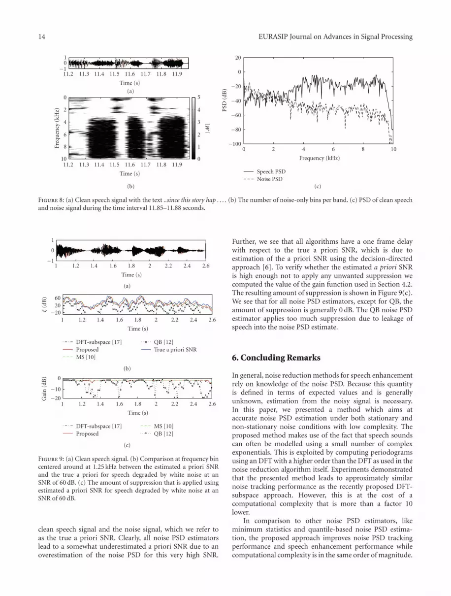
unvoiced sounds are especially dominantly present at higherfrequencies. Ideally, to prevent leakage of speech energy inthe noise PSD estimate, the noise PSD should not be updatedin this situation. The clean speech time-domain signal isshown in Figure 8(a); three noise bursts representing the /s/sounds are clearly visible. This signal is degraded by streetnoise at an SNR of 10 dB and processed using the proposednoise PSD estimator. The PSD of both the clean speech signaland the noise at the time interval 11.85 till 11.88 seconds areshown in Figure 8(c), where it is clearly visible that the speechsignal is dominant at higher frequencies. In Figure 8(b) weshow in the time-frequency plane for each frequency bandthe estimated number of noise-only bins in a band. We cansee that during the unvoiced speech sounds the cardinality


Table 4: Performance in terms of PESQ.

Noise source Input SNR (dB) MS [10] DFT-Sub. [17] Prop. method QB [12]

Pink noise

0 1.91 1.98 1.95 1.91

5 2.33 2.38 2.36 2.31

10 2.67 2.67 2.67 2.64

15 2.96 2.92 2.94 2.89

White noise

0 1.86 1.96 1.91 1.82

5 2.26 2.33 2.29 2.19

10 2.57 2.61 2.60 2.51

15 2.86 2.86 2.86 2.77

Party noise

0 1.62 1.63 1.66 1.63

5 2.02 2.05 2.07 2.02

10 2.40 2.43 2.44 2.39

15 2.74 2.75 2.78 2.72

waves at the beach

0 1.75 1.86 1.85 1.74

5 2.14 2.26 2.26 2.13

10 2.49 2.55 2.57 2.47

15 2.81 2.82 2.85 2.77

Circle saw

0 1.52 1.51 1.60 1.54

5 1.88 1.90 1.97 1.89

10 2.23 2.25 2.32 2.24

15 2.57 2.59 2.65 2.56

Passing train

0 1.87 1.96 1.97 1.89

5 2.26 2.34 2.36 2.28

10 2.62 2.65 2.69 2.61

15 2.93 2.91 2.96 2.88

passing cars

0 2.09 2.39 2.40 2.09

5 2.40 2.67 2.70 2.41

10 2.72 2.92 2.95 2.68

15 3.00 3.14 3.15 2.91

modulated white noise

0 1.59 1.97 1.92 1.64

5 1.98 2.33 2.29 2.02

10 2.34 2.60 2.60 2.37

15 2.68 2.86 2.86 2.67

modulated pink noise

0 1.75 2.00 1.97 1.79

5 2.14 2.38 2.37 2.18

10 2.50 2.66 2.67 2.52

15 2.83 2.91 2.93 2.81

of the set M(k, i), that is, the number of noise-only bins in aband, is determined to be |M(k, i)| = 0. Consequently, thenoise PSD is not updated at these time-frequency points.

5.3. Noise PSD Estimation in High SNR Situation. Althoughaccurate noise PSD estimation is important for applyingnoise reduction on noisy speech signals, it is also relevantto investigate the situation when very little noise is present.Clearly, the higher the SNR, the lower the noise-to-signalratio (NSR) and consequently a worse noise PSD estimate isto be expected. Obviously, for very high SNRs the noise PSDwill be overestimated due to leakage of speech energy intothe noise PSD estimate. However, the question is whether

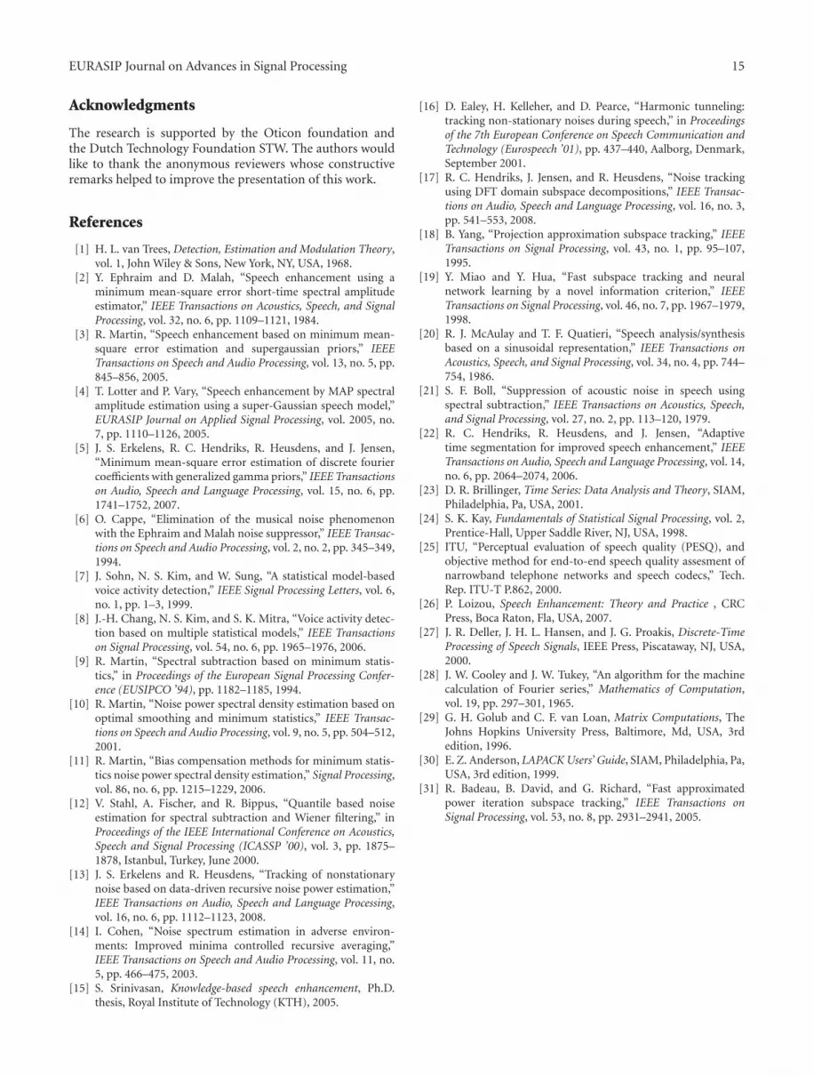
the level of the estimated noise PSD is low enough tonot influence the amount of suppression applied to thespeech signal afterwards by the noise suppression system.To investigate this situation, an experiment is performedwith a speech signal degraded by white noise at an SNRof 60 dB. Subsequently, the proposed noise PSD estimatorand the reference noise PSD estimators are applied to thissignal. The a priori SNR, defined as ξ(k, i) = σ2

X(k, i)/σ2N (k, i),

is estimated using the decision-directed approach [2] afterwhich it is used to compute the value of the gain functionused in Section 4. Figure 9(a) shows the original clean speechsignal. Figure 9(b) shows the estimated a priori SNRs in afrequency bin centered around 1.25 kHz. This is comparedwith the a priori SNR computed using knowledge of the


−101

11.2 11.3 11.4 11.5 11.6 11.7 11.8 11.9

Time (s)

(a)

(b) (c)

11.2 11.3 11.4 11.5 11.6 11.7 11.8 11.9

Time (s)

10

8

6

4

2

0

Fre

qu

ency

(kH

z)

0

1

2

3

4

5

|M|

−100

−80

−60

−40

−20

0

20

PSD

(dB

)

0 2 4 6 8 10

Frequency (kHz)

Speech PSD

Noise PSD

Figure 8: (a) Clean speech signal with the text ..since this story hap . . . . (b) The number of noise-only bins per band. (c) PSD of clean speechand noise signal during the time interval 11.85–11.88 seconds.

−1

0

1

1 1.2 1.4 1.6 1.8 2 2.2 2.4 2.6

Time (s)

(a)

−2020

60

ξ(d

B)

1 1.2 1.4 1.6 1.8 2 2.2 2.4 2.6

Time (s)

DFT-subspace [17]

Proposed

MS [10]

QB [12]

True a priori SNR

(b)

−20

−10

0

Gai

n(d

B)

1 1.2 1.4 1.6 1.8 2 2.2 2.4 2.6

Time (s)

DFT-subspace [17]

Proposed

MS [10]

QB [12]

(c)

Figure 9: (a) Clean speech signal. (b) Comparison at frequency bincentered around at 1.25 kHz between the estimated a priori SNRand the true a priori for speech degraded by white noise at anSNR of 60 dB. (c) The amount of suppression that is applied usingestimated a priori SNR for speech degraded by white noise at anSNR of 60 dB.

clean speech signal and the noise signal, which we refer toas the true a priori SNR. Clearly, all noise PSD estimatorslead to a somewhat underestimated a priori SNR due to anoverestimation of the noise PSD for this very high SNR.

Further, we see that all algorithms have a one frame delaywith respect to the true a priori SNR, which is due toestimation of the a priori SNR using the decision-directedapproach [6]. To verify whether the estimated a priori SNRis high enough not to apply any unwanted suppression wecomputed the value of the gain function used in Section 4.2.The resulting amount of suppression is shown in Figure 9(c).We see that for all noise PSD estimators, except for QB, theamount of suppression is generally 0 dB. The QB noise PSDestimator applies too much suppression due to leakage ofspeech into the noise PSD estimate.

6. Concluding Remarks

In general, noise reduction methods for speech enhancementrely on knowledge of the noise PSD. Because this quantityis defined in terms of expected values and is generallyunknown, estimation from the noisy signal is necessary.In this paper, we presented a method which aims ataccurate noise PSD estimation under both stationary andnon-stationary noise conditions with low complexity. Theproposed method makes use of the fact that speech soundscan often be modelled using a small number of complexexponentials. This is exploited by computing periodogramsusing an DFT with a higher order than the DFT as used in thenoise reduction algorithm itself. Experiments demonstratedthat the presented method leads to approximately similarnoise tracking performance as the recently proposed DFT-subspace approach. However, this is at the cost of acomputational complexity that is more than a factor 10lower.

In comparison to other noise PSD estimators, likeminimum statistics and quantile-based noise PSD estima-tion, the proposed approach improves noise PSD trackingperformance and speech enhancement performance whilecomputational complexity is in the same order of magnitude.


Acknowledgments

The research is supported by the Oticon foundation andthe Dutch Technology Foundation STW. The authors wouldlike to thank the anonymous reviewers whose constructiveremarks helped to improve the presentation of this work.

References

[1] H. L. van Trees, Detection, Estimation and Modulation Theory,vol. 1, John Wiley & Sons, New York, NY, USA, 1968.

[2] Y. Ephraim and D. Malah, “Speech enhancement using aminimum mean-square error short-time spectral amplitudeestimator,” IEEE Transactions on Acoustics, Speech, and SignalProcessing, vol. 32, no. 6, pp. 1109–1121, 1984.

[3] R. Martin, “Speech enhancement based on minimum mean-square error estimation and supergaussian priors,” IEEETransactions on Speech and Audio Processing, vol. 13, no. 5, pp.845–856, 2005.

[4] T. Lotter and P. Vary, “Speech enhancement by MAP spectralamplitude estimation using a super-Gaussian speech model,”EURASIP Journal on Applied Signal Processing, vol. 2005, no.7, pp. 1110–1126, 2005.

[5] J. S. Erkelens, R. C. Hendriks, R. Heusdens, and J. Jensen,“Minimum mean-square error estimation of discrete fouriercoefficients with generalized gamma priors,” IEEE Transactionson Audio, Speech and Language Processing, vol. 15, no. 6, pp.1741–1752, 2007.

[6] O. Cappe, “Elimination of the musical noise phenomenonwith the Ephraim and Malah noise suppressor,” IEEE Transac-tions on Speech and Audio Processing, vol. 2, no. 2, pp. 345–349,1994.

[7] J. Sohn, N. S. Kim, and W. Sung, “A statistical model-basedvoice activity detection,” IEEE Signal Processing Letters, vol. 6,no. 1, pp. 1–3, 1999.

[8] J.-H. Chang, N. S. Kim, and S. K. Mitra, “Voice activity detec-tion based on multiple statistical models,” IEEE Transactionson Signal Processing, vol. 54, no. 6, pp. 1965–1976, 2006.

[9] R. Martin, “Spectral subtraction based on minimum statis-tics,” in Proceedings of the European Signal Processing Confer-ence (EUSIPCO ’94), pp. 1182–1185, 1994.

[10] R. Martin, “Noise power spectral density estimation based onoptimal smoothing and minimum statistics,” IEEE Transac-tions on Speech and Audio Processing, vol. 9, no. 5, pp. 504–512,2001.

[11] R. Martin, “Bias compensation methods for minimum statis-tics noise power spectral density estimation,” Signal Processing,vol. 86, no. 6, pp. 1215–1229, 2006.

[12] V. Stahl, A. Fischer, and R. Bippus, “Quantile based noiseestimation for spectral subtraction and Wiener filtering,” inProceedings of the IEEE International Conference on Acoustics,Speech and Signal Processing (ICASSP ’00), vol. 3, pp. 1875–1878, Istanbul, Turkey, June 2000.

[13] J. S. Erkelens and R. Heusdens, “Tracking of nonstationarynoise based on data-driven recursive noise power estimation,”IEEE Transactions on Audio, Speech and Language Processing,vol. 16, no. 6, pp. 1112–1123, 2008.

[14] I. Cohen, “Noise spectrum estimation in adverse environ-ments: Improved minima controlled recursive averaging,”IEEE Transactions on Speech and Audio Processing, vol. 11, no.5, pp. 466–475, 2003.

[15] S. Srinivasan, Knowledge-based speech enhancement, Ph.D.thesis, Royal Institute of Technology (KTH), 2005.

[16] D. Ealey, H. Kelleher, and D. Pearce, “Harmonic tunneling:tracking non-stationary noises during speech,” in Proceedingsof the 7th European Conference on Speech Communication andTechnology (Eurospeech ’01), pp. 437–440, Aalborg, Denmark,September 2001.

[17] R. C. Hendriks, J. Jensen, and R. Heusdens, “Noise trackingusing DFT domain subspace decompositions,” IEEE Transac-tions on Audio, Speech and Language Processing, vol. 16, no. 3,pp. 541–553, 2008.

[18] B. Yang, “Projection approximation subspace tracking,” IEEETransactions on Signal Processing, vol. 43, no. 1, pp. 95–107,1995.

[19] Y. Miao and Y. Hua, “Fast subspace tracking and neuralnetwork learning by a novel information criterion,” IEEETransactions on Signal Processing, vol. 46, no. 7, pp. 1967–1979,1998.

[20] R. J. McAulay and T. F. Quatieri, “Speech analysis/synthesisbased on a sinusoidal representation,” IEEE Transactions onAcoustics, Speech, and Signal Processing, vol. 34, no. 4, pp. 744–754, 1986.

[21] S. F. Boll, “Suppression of acoustic noise in speech usingspectral subtraction,” IEEE Transactions on Acoustics, Speech,and Signal Processing, vol. 27, no. 2, pp. 113–120, 1979.

[22] R. C. Hendriks, R. Heusdens, and J. Jensen, “Adaptivetime segmentation for improved speech enhancement,” IEEETransactions on Audio, Speech and Language Processing, vol. 14,no. 6, pp. 2064–2074, 2006.

[23] D. R. Brillinger, Time Series: Data Analysis and Theory, SIAM,Philadelphia, Pa, USA, 2001.

[24] S. K. Kay, Fundamentals of Statistical Signal Processing, vol. 2,Prentice-Hall, Upper Saddle River, NJ, USA, 1998.

[25] ITU, “Perceptual evaluation of speech quality (PESQ), andobjective method for end-to-end speech quality assesment ofnarrowband telephone networks and speech codecs,” Tech.Rep. ITU-T P.862, 2000.

[26] P. Loizou, Speech Enhancement: Theory and Practice , CRCPress, Boca Raton, Fla, USA, 2007.

[27] J. R. Deller, J. H. L. Hansen, and J. G. Proakis, Discrete-TimeProcessing of Speech Signals, IEEE Press, Piscataway, NJ, USA,2000.

[28] J. W. Cooley and J. W. Tukey, “An algorithm for the machinecalculation of Fourier series,” Mathematics of Computation,vol. 19, pp. 297–301, 1965.

[29] G. H. Golub and C. F. van Loan, Matrix Computations, TheJohns Hopkins University Press, Baltimore, Md, USA, 3rdedition, 1996.

[30] E. Z. Anderson, LAPACK Users’ Guide, SIAM, Philadelphia, Pa,USA, 3rd edition, 1999.

[31] R. Badeau, B. David, and G. Richard, “Fast approximatedpower iteration subspace tracking,” IEEE Transactions onSignal Processing, vol. 53, no. 8, pp. 2931–2941, 2005.

Low Complexity DFT-Domain Noise PSD Tracking Using High-Resolution Periodograms

Documents