HAL Id: tel-01303774 https://tel.archives-ouvertes.fr/tel-01303774 Submitted on 18 Apr 2016 HAL is a multi-disciplinary open access archive for the deposit and dissemination of sci- entific research documents, whether they are pub- lished or not. The documents may come from teaching and research institutions in France or abroad, or from public or private research centers. L’archive ouverte pluridisciplinaire HAL, est destinée au dépôt et à la diffusion de documents scientifiques de niveau recherche, publiés ou non, émanant des établissements d’enseignement et de recherche français ou étrangers, des laboratoires publics ou privés. Lossy and lossless image coding with low complexity and based on the content Yi Liu To cite this version: Yi Liu. Lossy and lossless image coding with low complexity and based on the content. Signal and Image processing. INSA de Rennes; Rennes, INSA, 2015. English. NNT : 2015ISAR0028. tel- 01303774

Welcome message from author
This document is posted to help you gain knowledge. Please leave a comment to let me know what you think about it! Share it to your friends and learn new things together.
Transcript
HAL Id: tel-01303774https://tel.archives-ouvertes.fr/tel-01303774
Submitted on 18 Apr 2016
HAL is a multi-disciplinary open accessarchive for the deposit and dissemination of sci-entific research documents, whether they are pub-lished or not. The documents may come fromteaching and research institutions in France orabroad, or from public or private research centers.
L’archive ouverte pluridisciplinaire HAL, estdestinée au dépôt et à la diffusion de documentsscientifiques de niveau recherche, publiés ou non,émanant des établissements d’enseignement et derecherche français ou étrangers, des laboratoirespublics ou privés.
Lossy and lossless image coding with low complexity andbased on the content
Yi Liu
To cite this version:Yi Liu. Lossy and lossless image coding with low complexity and based on the content. Signal andImage processing. INSA de Rennes; Rennes, INSA, 2015. English. �NNT : 2015ISAR0028�. �tel-01303774�

THÈSE INSA Rennessous le sceau de l'Université Européenne de Bretagne
pour obtenir le grade de
DOCTEUR DE L'INSA DE RENNES
Spécialité : Traitement du Signal et des Images
présentée par
Yi LIU
ÉCOLE DOCTORALE : MATISSE
LABORATOIRE : IETR � UMR CNRS 6164
Codage d'imagesavec et sans pertes àbasse complexité et
basé contenu
Thèse soutenue le 18/03/2015
devant le jury composé de :
PUECH William
Professeur à l'Université de Montpellier / Président
MOKRAOUI Anissa
Professeure à l'Universtié Paris XIII / Rapporteuse
DUFAUX Frédéric
Directeur de Recherche à Telecom ParisTech / Rapporteur
LE MEUR Olivier
Maître de Conférences à l'Université de Rennes 1 / Examinateur
ZHANG Lu
Maître de Conférences à l'INSA de Rennes / Examinatrice
DEFORGES Olivier
Professeur à l'INSA de Rennes / Directeur de thèse

Codage d'images
avec et sans pertes à
basse complexité et
basé contenu
YI LIU
Document protégé par les droits d'auteur

Acknowledgments
I would like to thank Prof. MOKRAOUI Anissa, Prof. DUFAUX Frédéric, Prof. PUECH
William and Prof. LE MEUR Olivier for accepting to be members of the Ph.D. jury and taking
time to read and review this manuscript.
I would like to express my deep gratitude to my supervisor, Prof. Olivier Déforges, for
accepting me as a Ph.D student, for the resource and suggestion required to the work in this
thesis, and for a wider horizon of the topic of the thesis. His experience on research and patience
also made this thesis more valuable.
I would like to thank Dr. Lu Zhang for reading my manuscripts and offering valuable ad-
vices, and also thank Dr. Khouloud Samrouth and Dr. François Pasteau for the interpretation
and discussion during the work of the thesis.
Special thanks to the team IETR for the friendly and gentle support. Thanks Prof. Joseph
Ronsin and Luce Morin for providing reports and lectures, thanks Frédéric Garesché for solving
the technique problems.
Thanks to graduated Dr. Wenbin Zou, Dr. Weizhi Lu, Dr. Jinglin Zhang, Dr. Xiaohui Yi,
Dr. Yu Zhao, Dr. Cong Bai and Dr. Ming Liu for the help and advice on the research and
accommodation.
Special thanks to Wenjing Shuai for the encouragement and assistance. She gave me much
support and motivation during the work.
Thanks to Wei Liu, Han Yuan, Xiao Fan, Dandan Yao, Yang Yang, Qingyuan Gu, Zhigang
Yao, Liang Tang, Hua Fu, Jia Fu, Tian Xia, Shibo Liu, Yanping Wang, Jiali Xu, Xu Zhang,
Hengyang Wei, Hua Lu and friends for the pleasure time in Rennes.
Thanks to my parents, grandparents and other family members for the encouragement and
care every week.
Thanks to the China Scholarship Council for the support of the thesis.
Thanks to friendly French people for the help and pleasure time in France.
1

2 Acknowledgments
Résumé en français
Au cours de ces dernières décennies, l’image numérique en tant que média fut un moyen
particulièrement efficace pour le stockage et la transmission de l’information. Pour des uti-
lisations académiques, les documents, les archives d’art, et les images médicales ont été nu-
mérisés afin de faciliter le stockage et la recherche. En outre, la production massive d’images
numériques émerge dans les applications multimédias. Récemment, la société internet Yahoo
a affirmé que pas moins de 880 milliards photos ont été prises en 2014. Selon les sources is-
sues du SEC(U.S. Securities and Exchange Commission), plus de 250 millions des photos sont
téléchargées par Facebook tous les jours.
Afin de réduire les ressources de stockage pour la représentation d’une image, l’organisa-
tion internationale de normalisation (ISO) a établi et publié de nombreux standards de com-
pression d’image, tels que JPEG, JPEG, JPEG2000 et JPEG XR. En plus des normes, il existe
ensuite de nombreuses méthodes de compression efficaces, telles que CALIC ou SPIHT. Les
contributions présentées dans cette thèse se situent dans le contexte du codage LAR (Locally
Adaptive Resolution). Ce projet de recherche doctoral vise à proposer solution améliorée du
codec de codage d’images LAR, à la fois d’un point de vue des performances de compression
et de la complexité. L’étude présentée dans cette thèse concerne principalement les techniques
d’optimisation débit/distorsions (RDO) pour LAR. Avec un double objectif d’efficacité de co-
dage et de basse complexité, un nouveau schéma de codage LAR est également proposé dans
le mode sans perte (compression entièrement réversible).
Chapitre 1 la Technologie de Compression d’image
Afin de dresser le contexte de cette thèse, ce chapitre donne une introduction générale à la
compression d’image.
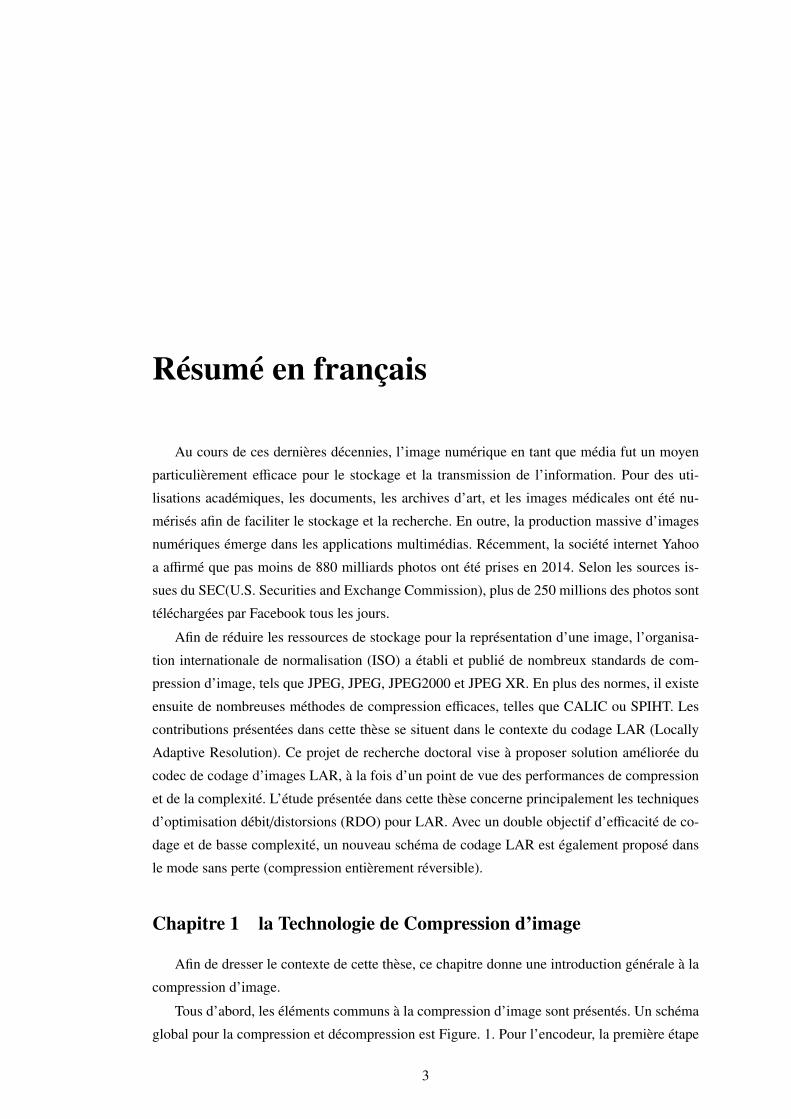
Tous d’abord, les éléments communs à la compression d’image sont présentés. Un schéma
global pour la compression et décompression est Figure. 1. Pour l’encodeur, la première étape
3
4 Résumé étendu en français
L’Image
originaleDécorrélation
Quantifica-
tion
Codage
entropique
Code flux
Décodage
entropique
Déquantifica-
tion
Décorrélation
inverse
L’image
récupérée
encodeur
décodeur
Imagecodeur
spatial
image basse
résolution+
+
- Texture codeur
spectral
Niveau l
Niveau l+1
Niveau l+2
1ère
pyramide2ère
pyramide
Transfor-
mation de
l’espace
de
couleur
Image
Prédiction
multi-niveaux
niveau n
niveau
n-1
...
niveau
1
Erreur de
prévision
Structure
pyramide
Luminance
Chrominance
Prédiction
multi-niveaux
niveau n
niveau
n-1
...
niveau
1
Structure
pyramide
Classification
niveau n
niveau
n - 1
niveau 1
...
Classification
niveau n
niveau
n - 1
niveau 1
...
Erreur de
prévision
......
Sub-
séquence
Codage
d’entropie
niveau n
niveau
n - 1
niveau 1
...
Codage
d’entropie
niveau n
niveau
n - 1
niveau 1
...
Assem
-blage
Flux
code
Sub-
séquence
Figure 1 – la procédure de la compression et la décompression d’image.
est la décorrélation qui permet de réduire la redondance spatiale. Cette redondance représente
la similitude des pixels locaux. Les techniques utilisées sont la prédiction, la transformation, la
mise en correspondance, etc. La deuxième étape, la quantification, est classiquement utilisée en
compression avec pertes. A l’issue de l’étape précédente, il existe de très nombreuses valeurs
autour de zéro, permettant de réduire la dynamique des coefficients, ce qui induit la redon-
dance statistique. Cette redondance est réduite par l’étape suivante, le codage de la entropie.
Le codage de Huffman, le codage arithmétique et le codage par plage sont les techniques cou-
ramment utilisées pour cette étape. Après la phase d’encodage, le flux est envoyé au décodeur
pour reconstruire l’image.
Dans un second temps, les techniques standards ou non de compression d’image sont pré-
sentées en tant que pratiques exemples de solutions. JPEG fut spécifié en 1991, et est basé sur
la transformée DCT (transformée en cosinus discrète). Le JPEG “classique” définit un proces-
sus de compression avec pertes. La partie de compression sans pertes fait l’objet d’une norme
spécifique appelée JPEG-LS qui utilise un algorithme différent de celui de JPEG. JPEGXR per-
met la compression avec perte ou sans pertes, et fut adopté comme norme en 2007. Il fournit
un format permettant la compression et la décompression en n’utilisant que des calculs sur des
entiers. JPEG2000 est aussi une norme commune à l’ISO et ITV, adopté en 2001. Il est capable
de compresser avec ou sans pertes, et se base principalement sur une transformée en ondelettes.
Les performances de JPEG 2000 en compression avec et sans pertes sont supérieures à celle
de la méthode de compression JPEG. Outre les normes, il excite des méthodes efficaces pour
Résumé étendu en français 5
la compression d’image, comme CALIC et SPIHT. CALIC (Context based Adaptive Lossless
Image Codec) permet de réaliser une compression sans perte uniquement, avec une efficacité
supérieure en comparaison avec méthodes standards, mais au prix d’une complexité de cal-
culs accrue. SPIHT (Set Partitioning in Hierarchical Trees) est un algorithme de compression
destiné à la compression des coefficients de la transformée en ondelettes. Il transforme progres-
sivement ces coefficients en un flux de bits. Au cours de décodage, les coefficients sont raffinés
plus en plus.
Enfin, nous présentons un test comparatif entre les performances des différents codecs
d’image. Pour la compression sans pertes, JPEG2000 propose la meilleure efficacité pour les
images couleur, et CALIC pour l’image en niveau gris. JPEG2000 et SPIHT obtiennent les
meilleurs résultats que les autres codecs pour la compression d’image avec pertes.
Chapitre 2 l’introduction de codec LAR
Plusieurs standards de compression d’images ont été proposés par le passé et mis à profit
dans de nombreuses applications multimedia, mais la recherche continue dans ce domaine afin
d’offrir de plus grande qualité de codage et/ou de plus faibles complexité de traitements. En
2008, le comité de standardisation JPEG a lancé un appel à proposition appelé AIC (Advanced
Image Coding). L’objectif était de pouvoir standardiser de nouvelles technologies allant au-
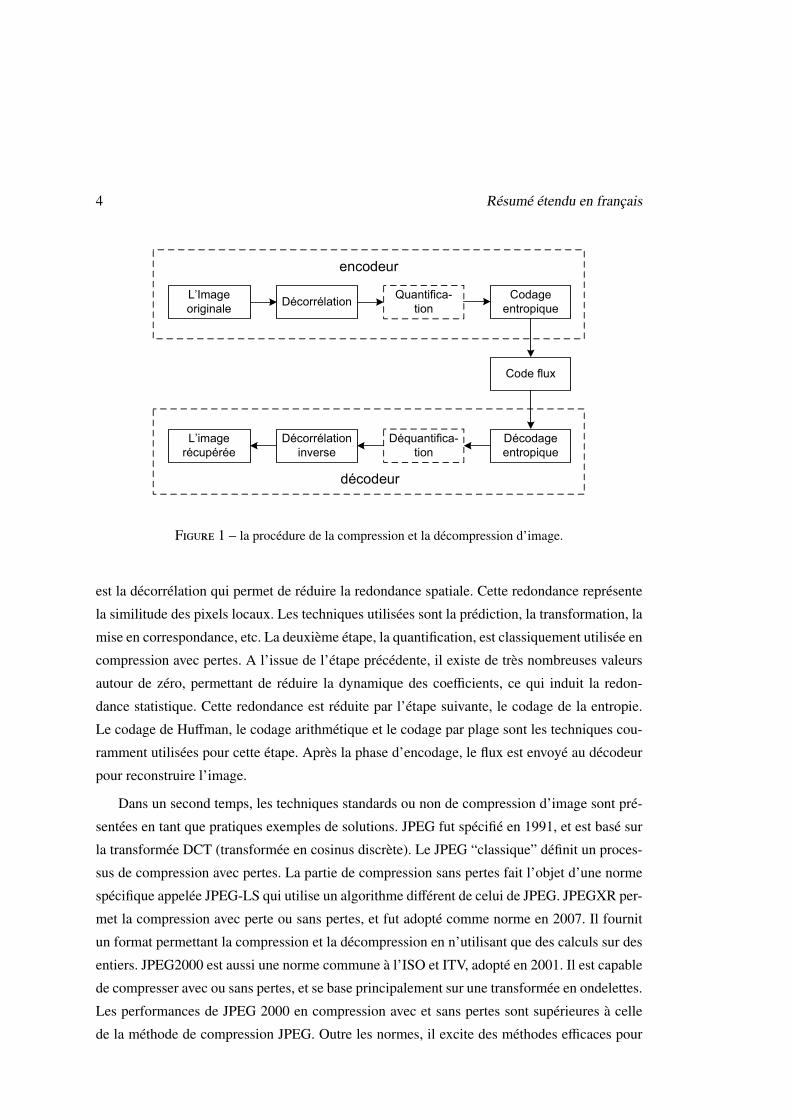
delà des standards existants. Le codec LAR fut alors proposé comme réponse à cet appel. Le
système LAR tend à associer une efficacité de compression et une représentation basée contenu.
Il supporte le codage avec et sans pertes avec la même structure.
Imagecodeur
spatial
image basse
résolution+
+
- Texture codeur
spectral
Figure 2 – LAR codec à deux couches
La méthode LAR est constituée d’un codec à deux couches : le codeur spatial, fournissant
une image basse résolution, et le codeur spectral traitant de la texture (Fig. 2). L’originalité de
l’algorithme repose sur le principe suivant : la résolution locale, i.e. la taille des pixels, peut
varier en fonction de l’activité locale. Ainsi, les pixels de petite taille se situent naturellement
sur les contours de l’image, alors que les zones uniformes sont représentées par un bloc de
grande taille. Cette grille de résolution spécifique s’appuyant sur le Quadtree déterminé par un
6 Résumé étendu en français
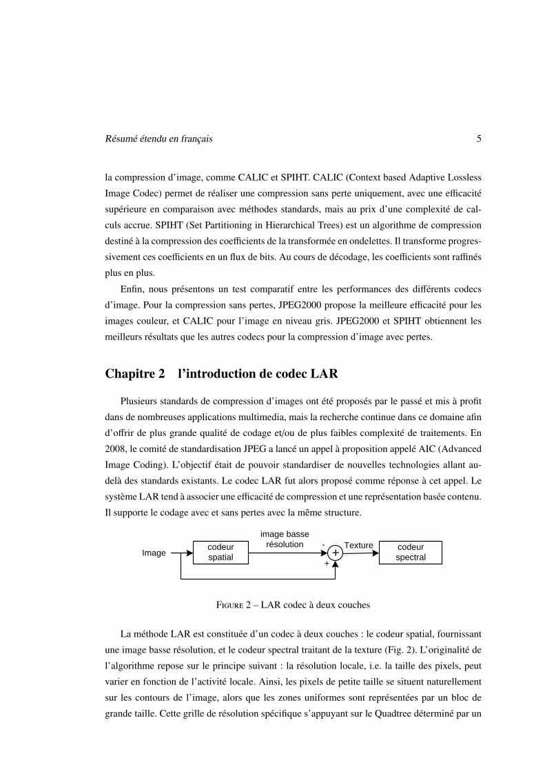
gradient morphologique. En outre, une technique, l’interleaved S+P, a été utilisée pour la pro-
priété de scalabilité de codage de la source. Elle est constituée de deux parties : la construction
et la décomposition de la pyramide.
Figure 3 – Construction de la pyramide par deux pyramides
Soit Y l’image originale de taille Nx × Ny, la représentation multirésolution d’une image
est donnée par l’ensemble {Il}lmaxl=0 , où lmax désigne le sommet de la pyramide et l = 0 la pleine
résolution. Quatre blocs sont représentés au niveau supérieur par un bloc de valeur égale à la
moyenne des deux blocs sous-jacents de la première diagonale (Fig. 3).I0(i, j) = Y(i, j), l = 0;
Il(i, j) =
⌊Il−1(2i, 2 j) + Il−1(2i + 1, 2 j + 1)
2
⌋, l > 0,
(1)
avec 0 ≤ i ≤ Nlx, 0 ≤ j ≤ Nl
y, où Nlx = Nx/l and Nl
y = Ny/l. La transformation de la deuxième
diagonale d’un bloc 2×2 donné peut en effet aussi être vue comme la réalisation d’une seconde
pyramide.
Le processus de décomposition dyadique de la pyramide résulte de l’extension de la mé-
thode de prédiction. Pour la première pyramide, la valeur de la moyenne étant déjà connue
(niveau supérieur de la première pyramide). Il faut ainsi estimer la valeur gradient de la pre-
mière diagonale d’un bloc 2 × 2 :
2Gl(i, j) =2.1[0.9Il+1(i, j) +
16
(Il(2i + 1, 2 j − 1) + Il(2i − 1, 2 j − 1)
+ Il(2i − 1, 2 j + 1))− 0.05
(Il(2i, 2 j − 2) + Il(2i − 2, 2 j)
)− 0.15
(Il+1(i, j + 1) + Il+1(i + 1, j)
)− Il+1(i, j)
] (2)
.
Résumé étendu en français 7
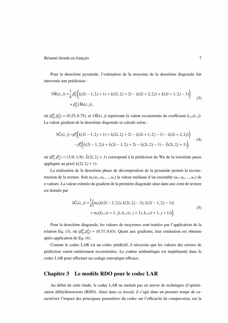
Pour la deuxième pyramide, l’estimation de la moyenne de la deuxième diagonale fait
intervenir une prédiction :
3Ml(i, j) =14β0
0
(Il(2i − 1, 2 j + 1) + Il(2i, 2 j + 2) − Il(2i + 2, 2 j) + Il(2i + 1, 2 j − 1)
)+ β1
0ˆ1Ml(i, j) ,
(3)
où (β00, β
10) = (0.25, 0.75), et 1Ml(i, j) représente la valeur reconstruite du coefficient Il+1(i, j).
La valeur gradient de la deuxième diagonale se calcule selon :
3Gl(i, j) =β01
(Il(2i − 1, 2 j + 1) + Il(2i, 2 j + 2) − Il(2i + 1, 2 j − 1) − Il(2i + 2, 2 j)
)− β0
1
(Il(2i − 1, 2 j) + Il(2i − 1, 2 j + 2) − Il(2i, 2 j − 1) − Il(2i, 2 j + 1)
),
(4)
où (β01, β
11) = (3/8, 1/8). Il(2i, 2 j + 1) correspond à la prédiction du Wu de la troisième passe
appliquée au pixel Il(2i, 2 j + 1).
La réalisation de la deuxième phase de décomposition de la pyramide permet la recons-
truction de la texture. Soit me(u1, u2, ..., un) la valeur médiane d’un ensemble (u1, u2, ..., un) de
n valeurs. La valeur estimée du gradient de la première diagonale situe dans une zone de texture
est donnée par
2Gt(i, j) =14
(me
(Il(2i − 2, 2 j), Il(2i, 2 j − 2), Il(2i − 1, 2 j − 1)
)+ me
(Il+1(i + 1, j), Il+1(i, j + 1), Il+1(i + 1, j + 1)
)).
(5)
Pour la deuxième diagonale, les valeurs de moyennes sont traitées par l’application de la
relation Eq. (3), où (β00, β
10) = (0.37, 0.63). Quant aux gradients, leur estimation est obtenue
après application de Eq. (4).
Comme le codec LAR est un codec prédictif, il nécessite que les valeurs des erreurs de
prédiction soient entièrement reconstruites. Le codeur arithmétique est implémenté dans le
codec LAR pour effectuer un codage entropique efficace.
Chapitre 3 Le modèle RDO pour le codec LAR
Au début de cette étude, le codec LAR ne mettait pas en œuvre de techniques d’optimi-
sation débit/distorsions (RDO). Ainsi dans ce travail, il s’agit dans un premier temps de ca-
ractériser l’impact des principaux paramètres du codec sur l’efficacité de compression, sur la
8 Résumé étendu en français
caractérisation des relations existantes entre efficacité de codage, puis de construire des mo-
dèles RDO pour la configuration des paramètres afin d’obtenir une efficacité de codage proche
de l’optimal.0 2 4 6 8 10 12 14
0
50
100
150
200
250
300
350
400
450
500
bpp
MS
Ebike crop
Distortion curve
Optimal point
Thr = 150
Thr = 90
Thr = 0
0 0.2 0.4 0.6 0.8 1 1.2 1.4 1.6
40
50
60
70
80
90
bpp
MS
E
bike crop
Distortion curve
Optimal point
0 50 100 150 200 2500
10
20
30
40
50
60
70
80
90
quqp
Th
r
Optimal pair
quqp = 53
Region I Region II
Figure 4 – Combinaisons optimales des paramètres pour ’bike crop’
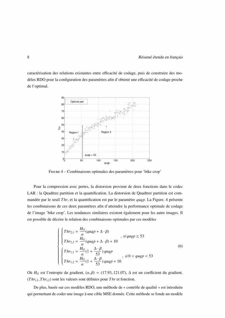
Pour la compression avec pertes, la distorsion provient de deux fonctions dans le codec
LAR : la Quadtree partition et la quantification. La distorsion de Quadtree partition est com-
mandée par le seuil Thr, et la quantification est par le paramètre quqp. La Figure. 4 présente
les combinaisons de ces deux paramètres afin d’atteindre la performance optimale de codage
de l’image ’bike crop’. Les tendances similaires existent également pour les autre images. Il
est possible de décrire le relation des combinaisons optimales par ces modèles
Thr2,1 =
HG
α(quqp + ∆ · β)
Thr2,2 =HG
α(quqp + ∆ · β) + 10
, si quqp ≥ 53
Thr1,1 =
HG
α(1 +
∆ · β
53) quqp
Thr1,2 =HG
α(1 +
∆ · β
53) quqp + 10
, si 0 < quqp < 53
(6)
Où HG est l’entropie du gradient, (α, β) = (17.93, 121.07), ∆ est un coefficient du gradient.
(Thri,1,Thri,2) sont les valeurs sont définies pour Thr et fonction.
De plus, basée sur ces modèles RDO, une méthode de « contrôle de qualité » est introduite
qui permettant de coder une image à une cible MSE donnée. Cette méthode se fonde un modèle
Résumé étendu en français 9
(a) appliqués localement
(b) appliqués globalement
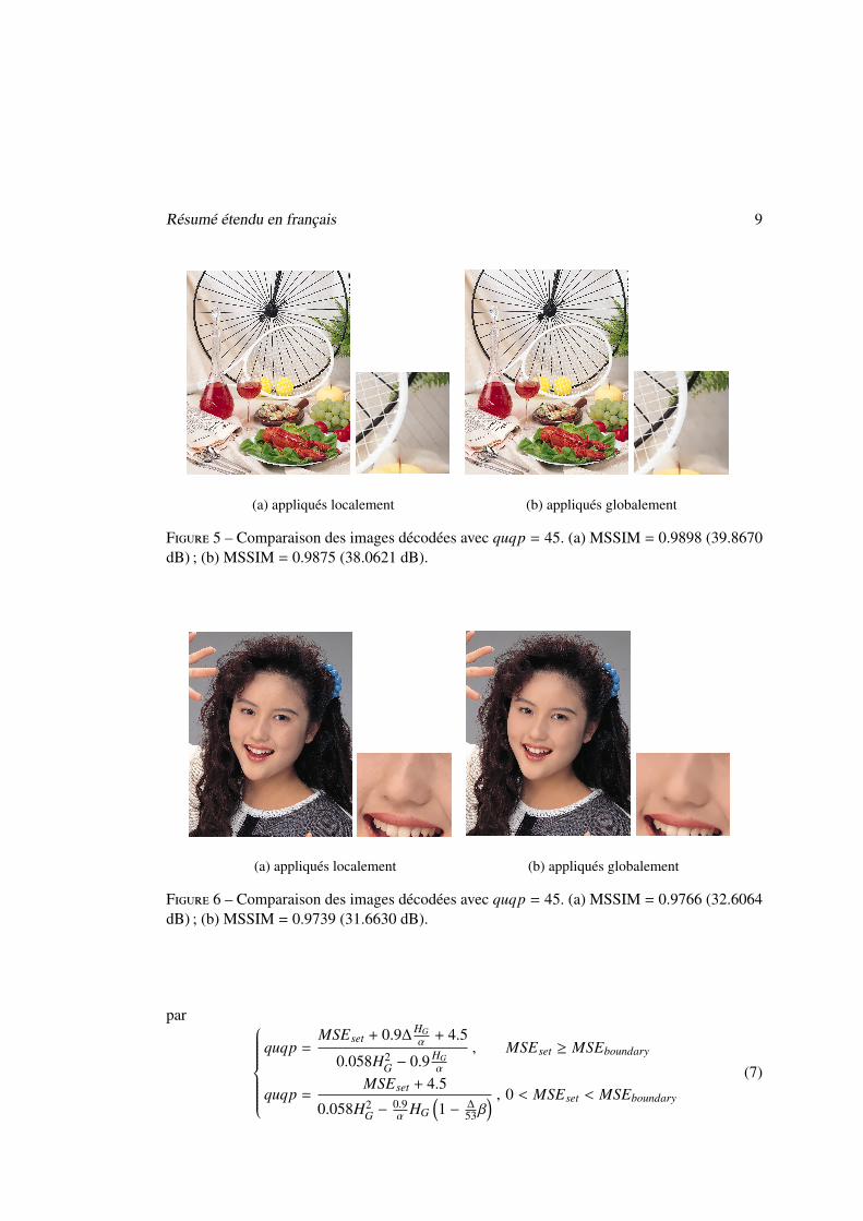
Figure 5 – Comparaison des images décodées avec quqp = 45. (a) MSSIM = 0.9898 (39.8670dB) ; (b) MSSIM = 0.9875 (38.0621 dB).
(a) appliqués localement
(b) appliqués globalement
Figure 6 – Comparaison des images décodées avec quqp = 45. (a) MSSIM = 0.9766 (32.6064dB) ; (b) MSSIM = 0.9739 (31.6630 dB).
par quqp =
MSEset + 0.9∆HGα + 4.5
0.058H2G − 0.9 HG
α
, MSEset ≥ MSEboundary
quqp =MSEset + 4.5
0.058H2G −
0.9α HG
(1 − ∆
53β) , 0 < MSEset < MSEboundary
(7)
10 Résumé étendu en français
Imagecodeur
spatial
image basse
résolution+
+
- Texture codeur
spectral
Niveau l
Niveau l+1
Niveau l+2
1ère
pyramide2ère
pyramide
Transfor-
mation de
l’espace
de
couleur
Image
Prédiction
multi-niveaux
niveau n
niveau
n-1
...
niveau
1
Erreur de
prévision
Structure
pyramide
Luminance
Chrominance
Prédiction
multi-niveaux
niveau n
niveau
n-1
... niveau
1
Structure
pyramide
Classification
niveau n
niveau
n - 1
niveau 1
...
Classification
niveau n
niveau
n - 1
niveau 1
...
Erreur de
prévision
......
Sub-
séquence
Codage
d’entropie
niveau n
niveau
n - 1
niveau 1
...
Codage
d’entropie
niveau n
niveau
n - 1
niveau 1
...
Assem
-blage
Flux
code
Sub-
séquence
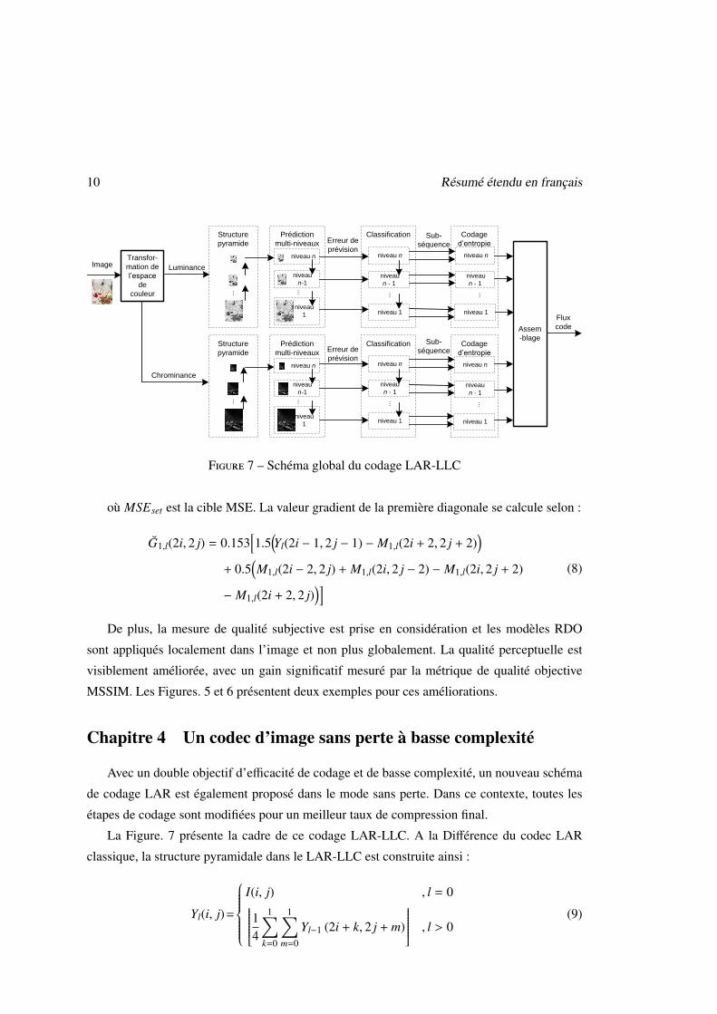
Figure 7 – Schéma global du codage LAR-LLC
où MSEset est la cible MSE. La valeur gradient de la première diagonale se calcule selon :
G1,l(2i, 2 j) = 0.153[1.5
(Yl(2i − 1, 2 j − 1) − M1,l(2i + 2, 2 j + 2)
)+ 0.5
(M1,l(2i − 2, 2 j) + M1,l(2i, 2 j − 2) − M1,l(2i, 2 j + 2)
− M1,l(2i + 2, 2 j))] (8)
De plus, la mesure de qualité subjective est prise en considération et les modèles RDO
sont appliqués localement dans l’image et non plus globalement. La qualité perceptuelle est
visiblement améliorée, avec un gain significatif mesuré par la métrique de qualité objective
MSSIM. Les Figures. 5 et 6 présentent deux exemples pour ces améliorations.
Chapitre 4 Un codec d’image sans perte à basse complexité
Avec un double objectif d’efficacité de codage et de basse complexité, un nouveau schéma
de codage LAR est également proposé dans le mode sans perte. Dans ce contexte, toutes les
étapes de codage sont modifiées pour un meilleur taux de compression final.
La Figure. 7 présente la cadre de ce codage LAR-LLC. A la Différence du codec LAR
classique, la structure pyramidale dans le LAR-LLC est construite ainsi :
Yl(i, j)=
I(i, j) , l = 014
1∑k=0
1∑m=0
Yl−1 (2i + k, 2 j + m)
, l > 0(9)
Résumé étendu en français 11
Où 0 ≤ i ≤ Nx/2l. b.c signifie l’arrondi vers le bas.
Pour la prédiction multi-niveaux, l’estimation de la moyenne des deux diagonales est
Gd,l(2i, 2 j) =α
4
(Gd,l(2i − 2, 2 j − 2) + Gd,l(2i + 2, 2 j − 2)
)+ β
(Yl+1(i − 1, j − 1) + Yl+1(i + 1, j + 1)
− Yl+1(i − 1, j + 1) − Yl+1(i + 1, j − 1)) (10)
Où α = 0.3, β = 0.035. L’estimation de la gradient de la première diagonale fait intervenir une
prédiction :
G1,l(2i, 2 j) = 0.153[1.5
(Yl(2i − 1, 2 j − 1) − M1,l(2i + 2, 2 j + 2)
)+ 0.5
(M1,l(2i − 2, 2 j) + M1,l(2i, 2 j − 2) − M1,l(2i, 2 j + 2)
− M1,l(2i + 2, 2 j))] (11)
La valeur gradient de la deuxième diagonale se calcule selon :
G2,l(2i, 2 j) =α
2
(Yl(2i, 2 j) − Yl(2i − 1, 2 j + 1) + Yl(2i + 2, 2 j) − Yl(2i + 1, 2 j + 1)
)+
1 − α2
(Yl(2i + 1, 2 j − 1) − Yl(2i, 2 j) + Yl(2i + 1, 2 j + 1)
− Yl(2i, 2 j + 2)) (12)
Où
G2,l(2i, 2 j) =38
(Yl(2i + 1, 2 j − 1) + Yl(2i + 2, 2 j) − Yl(2i − 1, 2 j + 1) − Yl(2i, 2 j + 2)
)−
18
(Yl(2i, 2 j − 1) + Yl(2i + 2, 2 j − 1) − Yl(2i − 1, 2 j) − Xl(2i + 1, 2 j)
) (13)
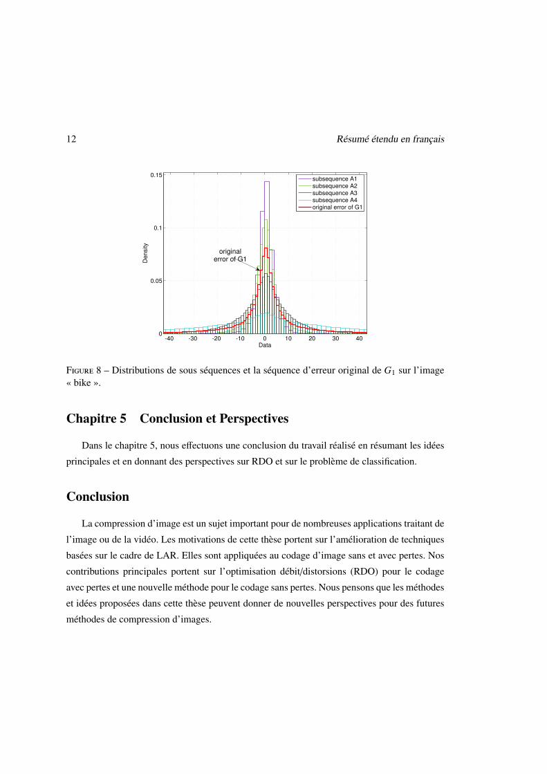
Après la prédiction, les erreurs sont classées en quatre groupes, afin de réduire l’entropie
de la séquence à coder. Cette classification se fonde sur le fait que l’entropie de la source
diminue quand la source est séparée en deux sous-sources avec les différentes distributions de
probabilité. La Figure. 8 présente un exemple pour la gradient de la première diagonale de
l’image « bike ».
Le LAR-LLC utilise le codeur Huffman pour effectuer un codage entropique efficace.
12 Résumé étendu en français
-40 -30 -20 -10 0 10 20 30 400
0.05
0.1
0.15
Data
De
nsity
subsequence A1subsequence A2subsequence A3subsequence A4original error of G1
originalerror of G1
Figure 8 – Distributions de sous séquences et la séquence d’erreur original de G1 sur l’image« bike ».
Chapitre 5 Conclusion et Perspectives
Dans le chapitre 5, nous effectuons une conclusion du travail réalisé en résumant les idées
principales et en donnant des perspectives sur RDO et sur le problème de classification.
Conclusion
La compression d’image est un sujet important pour de nombreuses applications traitant de
l’image ou de la vidéo. Les motivations de cette thèse portent sur l’amélioration de techniques
basées sur le cadre de LAR. Elles sont appliquées au codage d’image sans et avec pertes. Nos
contributions principales portent sur l’optimisation débit/distorsions (RDO) pour le codage
avec pertes et une nouvelle méthode pour le codage sans pertes. Nous pensons que les méthodes
et idées proposées dans cette thèse peuvent donner de nouvelles perspectives pour des futures
méthodes de compression d’images.
Contents
Acknowledgments 1
Contents 13
Introduction 17
1 Image compression technology 21
1.1 Common approaches in image compression . . . . . . . . . . . . . . . . . . . 22
1.1.1 Prediction . . . . . . . . . . . . . . . . . . . . . . . . . . . . . . . . . 22
1.1.2 Transform . . . . . . . . . . . . . . . . . . . . . . . . . . . . . . . . . 23
1.1.3 Matching . . . . . . . . . . . . . . . . . . . . . . . . . . . . . . . . . 25
1.1.4 Scalar Quantization . . . . . . . . . . . . . . . . . . . . . . . . . . . . 27
1.1.5 Variable length coding . . . . . . . . . . . . . . . . . . . . . . . . . . 27
1.1.6 Conclusion of common methods . . . . . . . . . . . . . . . . . . . . . 29
1.2 Still image coding standards . . . . . . . . . . . . . . . . . . . . . . . . . . . 29
1.2.1 JPEG . . . . . . . . . . . . . . . . . . . . . . . . . . . . . . . . . . . 29
1.2.2 JPEG-LS . . . . . . . . . . . . . . . . . . . . . . . . . . . . . . . . . 30
1.2.3 JPEG2000 . . . . . . . . . . . . . . . . . . . . . . . . . . . . . . . . 31
1.2.4 JPEGXR . . . . . . . . . . . . . . . . . . . . . . . . . . . . . . . . . 35
1.3 Nonstandard still image coding methods . . . . . . . . . . . . . . . . . . . . . 36
1.3.1 CALIC . . . . . . . . . . . . . . . . . . . . . . . . . . . . . . . . . . 36
1.3.2 SPIHT . . . . . . . . . . . . . . . . . . . . . . . . . . . . . . . . . . 38
1.4 Image compression performance . . . . . . . . . . . . . . . . . . . . . . . . . 40
1.4.1 Lossy compression performance . . . . . . . . . . . . . . . . . . . . . 40
1.4.2 Lossless compression performance . . . . . . . . . . . . . . . . . . . . 42
1.5 LAR codec for JPEG-AIC Response . . . . . . . . . . . . . . . . . . . . . . . 43
13
14 Contents
2 Introduction to LAR codec 45
2.1 Quadtree Partitioning . . . . . . . . . . . . . . . . . . . . . . . . . . . . . . . 46
2.2 Interleaved Pyramid Construction . . . . . . . . . . . . . . . . . . . . . . . . 47
2.3 Pyramid Decomposition and Prediction Model . . . . . . . . . . . . . . . . . . 49
2.3.1 LAR block process . . . . . . . . . . . . . . . . . . . . . . . . . . . . 50
2.3.2 Texture block process . . . . . . . . . . . . . . . . . . . . . . . . . . . 51
2.4 Quantization . . . . . . . . . . . . . . . . . . . . . . . . . . . . . . . . . . . . 51
2.5 Entropy coding . . . . . . . . . . . . . . . . . . . . . . . . . . . . . . . . . . 52
2.6 Conclusion . . . . . . . . . . . . . . . . . . . . . . . . . . . . . . . . . . . . 53
3 Rate-distortion-optimization (RDO) model for LAR codec 55
3.1 Parameter effects on distortion . . . . . . . . . . . . . . . . . . . . . . . . . . 56
3.2 Optimal Thr-quqp model . . . . . . . . . . . . . . . . . . . . . . . . . . . . . 58
3.3 Experiment of the RDO model . . . . . . . . . . . . . . . . . . . . . . . . . . 64
3.4 Quality Control . . . . . . . . . . . . . . . . . . . . . . . . . . . . . . . . . . 70
3.4.1 MSE Determination Model . . . . . . . . . . . . . . . . . . . . . . . 71
3.4.2 MSE constraint method . . . . . . . . . . . . . . . . . . . . . . . . . 72
3.4.3 Experiments of the MSE setting method . . . . . . . . . . . . . . . . . 74
3.5 Locally perceptual quality enhancement . . . . . . . . . . . . . . . . . . . . . 76
3.5.1 Adaptive Thr allocation scheme . . . . . . . . . . . . . . . . . . . . . 78
3.5.2 The Structure Similarity (SSIM) quality assessment . . . . . . . . . . . 79
3.5.3 Experiments of the adaptive Thr allocation scheme . . . . . . . . . . . 84
3.6 Conclusion . . . . . . . . . . . . . . . . . . . . . . . . . . . . . . . . . . . . 89
4 A low complexity lossless image codec : LAR-LLC 91
4.1 Framework of Coding Scheme . . . . . . . . . . . . . . . . . . . . . . . . . . 93
4.2 HD-ST Transform and Pyramid . . . . . . . . . . . . . . . . . . . . . . . . . 94
4.3 Pyramidal Prediction . . . . . . . . . . . . . . . . . . . . . . . . . . . . . . . 97
4.3.1 Prediction for Gd,l . . . . . . . . . . . . . . . . . . . . . . . . . . . . 98
4.3.2 Prediction for G1,l . . . . . . . . . . . . . . . . . . . . . . . . . . . . 98
4.3.3 Prediction for G2,l . . . . . . . . . . . . . . . . . . . . . . . . . . . . 100
4.4 Entropy Pre-coding and Coding of Prediction Errors . . . . . . . . . . . . . . . 102
4.5 Compression Performance . . . . . . . . . . . . . . . . . . . . . . . . . . . . 107
4.5.1 Compression Efficiency . . . . . . . . . . . . . . . . . . . . . . . . . 107
4.5.2 Computation Complexity . . . . . . . . . . . . . . . . . . . . . . . . . 112
Contents 15
4.6 Conclusion . . . . . . . . . . . . . . . . . . . . . . . . . . . . . . . . . . . . 115
5 Conclusion and Perspectives 117
5.1 Conclusion of the thesis work . . . . . . . . . . . . . . . . . . . . . . . . . . . 117
5.1.1 Rate-distortion-optimization model for LAR codec . . . . . . . . . . . 117
5.1.2 Lossless Low-complexity codec LAR-LLC . . . . . . . . . . . . . . . 118
5.2 Perspectives . . . . . . . . . . . . . . . . . . . . . . . . . . . . . . . . . . . . 119
5.2.1 Distortion control based on the perceptual quality in the lossy coding . 119
5.2.2 Better context model for the classification in the Pre-coding process . . 120
Glossary 121
Publication 123
Bibliography 134

16 Contents
Introduction
In nowadays, digital images are commonly captured by digital cameras, smart-phones, ta-
blets and so on. The main usage of the digital image is to record the visual information for the
conservation and communication. In the academic field, the digital imaging has been a practi-
cal tool for the storage of important documents, art archives, and medical images. Besides, the
massive production of digital images emerges in multimedia applications. The internet corpora-
tion Yahoo claimed that as many as 880 billion photos were taken in 2014 [pop13]. According
to the quote directly from the SEC doc [SC12], on average more than 250 million photos per
day were uploaded to Facebook in the three months ended December 31, 2011. That’s almost
3,000 photos per second. All those photos take up a lot of space on servers, stored more than
100 petabytes (100 million gigabytes) [pop12]. Meanwhile, for popular photo sharing games,
the transmission of digital images also occupies the bandwidth of the telecommunication.
In this context, the image compression technique is required. The aim of this technique
is to reduce the bit resource for the representation of an image. In practical cases, the image
compression codec should be able to perform lossless and lossy compressions. The lossless
coding is mainly used for the original archive and other important cases where any losses are
not allowed. The lossy coding aims at a high compression ratio and is commonly applied to
the commercial multimedia, such as videos and images for the entertainment in internet. In
the case of social networking, different targeted devices exhibiting different screen resolutions
have to be considered. Moreover, those terminals have also different computational abilities.
Therefore, there is a need for the codec with both resolution and computation scalability.
With the development of digital cameras, computer entertainments and internet commu-
nications, different image codecs have been proposed. The mostly used one is JPEG which
has been standardized by the JPEG committee in 1992 [CCI92]. It is based on the Discrete
Cosine Transform (DCT) with a dedicated quantization process. This coding method has a
low computational complexity and has been well implemented in both software and hardware.
The drawbacks are the limited quality of the decoded image and the lack of the lossless co-
17
18 Introduction
ding function. For the lossless function, JPEG-LS was standardized in 1998 [IT98]. It adopts
a predictive coding method which is different from the JPEG. In 2002, JPEG committee stan-
dardized JPEG2000 which supports both the lossy and the lossless coding [IT02]. Compared
with JPEG, its decoded images have better objective qualities, such as PSNR, at the same com-
pression ratios. Besides, JPEG2000 supports the multiresolution, the rate control functions and
so on. However, JPEG2000 requires high computation, limiting its application. Then, JPEG
XR was created by Microsoft and standardized in 2009 [ISO09]. It has a lower computational
complexity than that of JPEG2000 and better coding quality than JPEG.
Besides these standards, other image coding methods were proposed to improve the com-
pression performance such as CALIC and SPIHT which are introduced in Section 1.3. The
LAR (Locally Adaptive Resolution) codec, which is explained in Chapter 2, was also designed
as an image coding solution. It is the base for the study in this thesis.
The contributions presented in this thesis aim at the improvement of the coding perfor-
mance of the LAR codec. Although the LAR codec has a complete structure, its coding steps
are still under a rough configuration and need a further analysis to achieve a preferable perfor-
mance. The first research aims at the study of the distortion caused by different configurations.
This work gives a better choice of parameters for the rate distortion optimization. The second
research focuses on a more efficient coding solution with a low computational cost.
The thesis is organized as follows. The commonly used image compression methods are
firstly presented in Chapter 1. Next, Chapter 2 introduces the LAR codec. The rate distor-
tion optimization scheme for the LAR codec is proposed in Chapter 3. In Chapter 4, the low-
complexity lossless image codec is designed and tested. Finally, the conclusion and prospects
are presented in Chapter 5.
1 Image compression technology
The commonly applied image coding structure and methods are presented. Based on these
methods, the standardized schemes and some non-standardized codecs are briefly introduced.
Their lossy and lossless coding performance finally are compared respectively.
2 Introduction to LAR codec
The coding steps of the LAR codec are presented. In this chapter, the framework of the
LAR codec is introduced step by step. The quadtree partition is firstly used to detect the local
activity of pixels of the image and draw a quadtree map which is determined by a threshold.
Based on the map, the image is degraded from the full resolution to lower resolutions level
Introduction 19
by level, generating to a pyramidal structure. Then, a decomposition starts from the lowest
resolution level to higher resolution levels, until the full resolution image is reconstructed.
The prediction and the quantization of the prediction errors are used in the decomposition.
Finally, the quantized prediction errors are coded. Although the LAR has the complete coding
framework, the coding parameters have not been well configured to find the optimal coding
performance. In order to relieve this limitation, a Rate-Distortion-Optimization (RDO) model
is proposed in Chapter 3.
3 Rate-Distortion-Optimization (RDO) model for LAR codec
In this chapter, the distortions caused by the change of the quantization factor and the
quadtree partition threshold are studied to understand the rate-distortion performance of the
LAR codec. Next, the relationship between the optimal coding efficiency and changes of the
parameters are analyzed in order to propose a RDO model for the LAR codec. The RDO model
is tested and the experimental results are discussed. Based on the RDO model, a linear quality
control (QC) model is also built. This QC model is used to constraint the distortion of the coded
image to the target one which is set before the coding by the user. Besides, a locally adaptive
scheme of the RDO model is proposed to improve the perceptual quality of the decoded image.
Finally, the coding performance of optimized LAR codec is compared with other image coding
schemes.
4 A low complexity lossless image codec : LAR-LLC
The LAR codec has the lossless coding function. However, the coding performance is not as
efficient as the one of JPEG2000. Therefore, we propose a new lossless coding method aiming
at improving the compression ratio and reducing the computational complexity. This method
still uses the framework of the LAR, but changes each coding steps. It adopts a new transform
for the resolution scalability and reconstructs images in different resolutions according to new
context models for prediction. Besides, it exploits the remaining correlation of the prediction
errors, and a classification process is proposed to improve the compression efficiency. Finally
the lossless coding efficiency of the codec is compared with standard codecs and recently pro-
posed image codecs.
5 Conclusion and Prospects
The contributions of the thesis are based on a predictive image codec. An RDO model is
firstly proposed to this codec, then a quality constraint scheme and a locally subjective quality
20 Introduction
enhancement scheme are introduced. After, a new complete lossless image coding method is
proposed to achieve an efficient compression ratio with a low computational complexity.
Thanks to the study presented in this thesis, different ideas are proposed as prospects for
the image coding. Firstly a scheme of the lossy coding based on the characters of the Human
Visual System is designed. This envisage can be seen as an extension of the locally adaptive
scheme of the RDO model introduced in Chapter 3, but the idea can be a reference for other
image coding solutions. Another idea is to improve the efficiency of the classification step used
in the lossless codec introduced in Chapter 4. More analysis and experiments are required to
design a new pre-coding scheme.
Chapter 1
Image compression technology
Modern industry employs images extensively. As an important medium, the image is a
common form used for the storage and transmission of the visual information. Besides the
traditional photography, the image is also applied for the technical drawing, art archiving, me-
dical imaging, film production and so on. These extensive applications bring a massive storage
of images. This requirement encourages researchers on the image compression technology to
make use of the limited storage and communication capacity efficiently.
A digital image is a rectangular array of picture elements, arranged in m rows and n
columns. The size m × n refers to the resolution of the image and the elements are called
pixels. In an image, especially for the natural image, some adjacent pixels probably have the
same or very similar colors. These pixels are highly correlated. This correlation is also cal-
led spatial redundancy. Image compression technologies mainly focus on the reduction of the
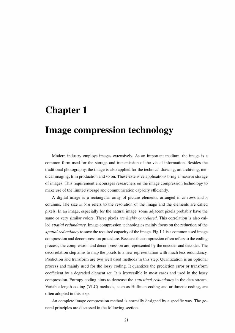
spatial redundancy to save the required capacity of the image. Fig.1.1 is a common used image
compression and decompression procedure. Because the compression often refers to the coding
process, the compression and decompression are represented by the encoder and decoder. The
decorrelation step aims to map the pixels to a new representation with much less redundancy.
Prediction and transform are two well used methods in this step. Quantization is an optional
process and mainly used for the lossy coding. It quantizes the prediction error or transform
coefficient by a degraded element set. It is irreversible in most cases and used in the lossy
compression. Entropy coding aims to decrease the statistical redundancy in the data stream.
Variable length coding (VLC) methods, such as Huffman coding and arithmetic coding, are
often adopted in this step.
An complete image compression method is normally designed by a specific way. The ge-
neral principles are discussed in the following section.
21
22 chapter 1
Original
imageDecorrelation Quantization
Entropy
coding
Code stream
Entropy
decoding
De-
quantization
Inverse
decorrelation
Recovered
image
encoder
decoder
Figure 1.1 – Image compression and decompression procedure.
1.1 Common approaches in image compression
1.1.1 Prediction
Original
imageDecorrelation Quantization
Entropy
coding
Code stream
Entropy
decoding
De-
quantization
Inverse
decorrelation
Recovered
image
encoder
decoder
Xi
...
...
Yi-1Yi-2
Yi-3Yi-4Yi-5Yi-6Yi-7
Yi-8Yi-9Yi-10Yi-11Yi-12 Reference
space
Predicted
pixel
Figure 1.2 – Pixels for prediction.
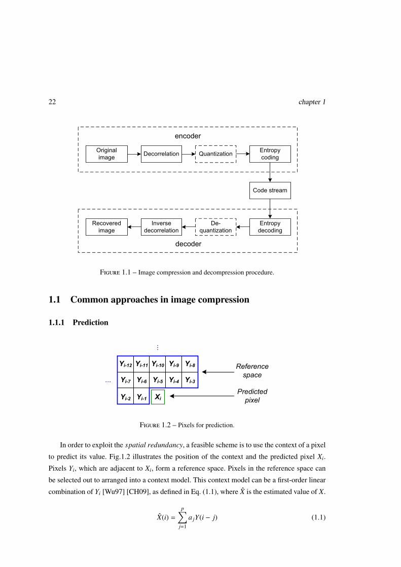
In order to exploit the spatial redundancy, a feasible scheme is to use the context of a pixel
to predict its value. Fig.1.2 illustrates the position of the context and the predicted pixel Xi.
Pixels Yi, which are adjacent to Xi, form a reference space. Pixels in the reference space can
be selected out to arranged into a context model. This context model can be a first-order linear
combination of Yi [Wu97] [CH09], as defined in Eq. (1.1), where X is the estimated value of X.
X(i) =
p∑j=1
a jY(i − j) (1.1)
Common approaches in image compression 23
The linear model is easy to calculate. However, the correlation between X and Y is variable
and probably not linear. One solution is to use non-linear model [ZM04]. This model adopts two
or higher order relations to describe the non linear correlation. Another solution is still apply
the linear one, but select it from a linear context model set [PKC+10]. Both solutions make
efforts to give a precise predicted value for Xi. It leads to a low amplitude prediction error for
each pixel. The reason why the prediction is helpful for the compression can be shown by the
change of entropy. Assuming that the pixel of the image is from a set of X = {X1, X2, X3, ..., Xn},
the probability of occurrence of X is {p1, p2, p3, ..., pn}. The uncertainty of the pixel can be
represented by the entropy H(X).
H(X) = H(p1, p2, p3, ..., pn) = −
n∑i=1
pi log pi (1.2)
If we consider the pixels Y of the reference space in order to predict X, the image entropy
becomes H(X|Y). It means the uncertainty of X when Y has been known. Because after pre-
diction, the prediction error replaces the pixel, H(X|Y) can also be seen as the entropy of the
prediction error. In information theory, it exits that
H(X|Y) ≤ H(X) (1.3)
and the equality exits only when Y is independent to X. Because Y is correlated to X, H(X|Y)
must be less than H(X). Another fact is that the entropy also represents the required least
average codeword length by the entropy coding. Thus, after the prediction step, the information
of the image needs less codeword resource than that without the prediction by the entropy
coding. As a result, the prediction is an effective process to reduce the spatial redundancy.
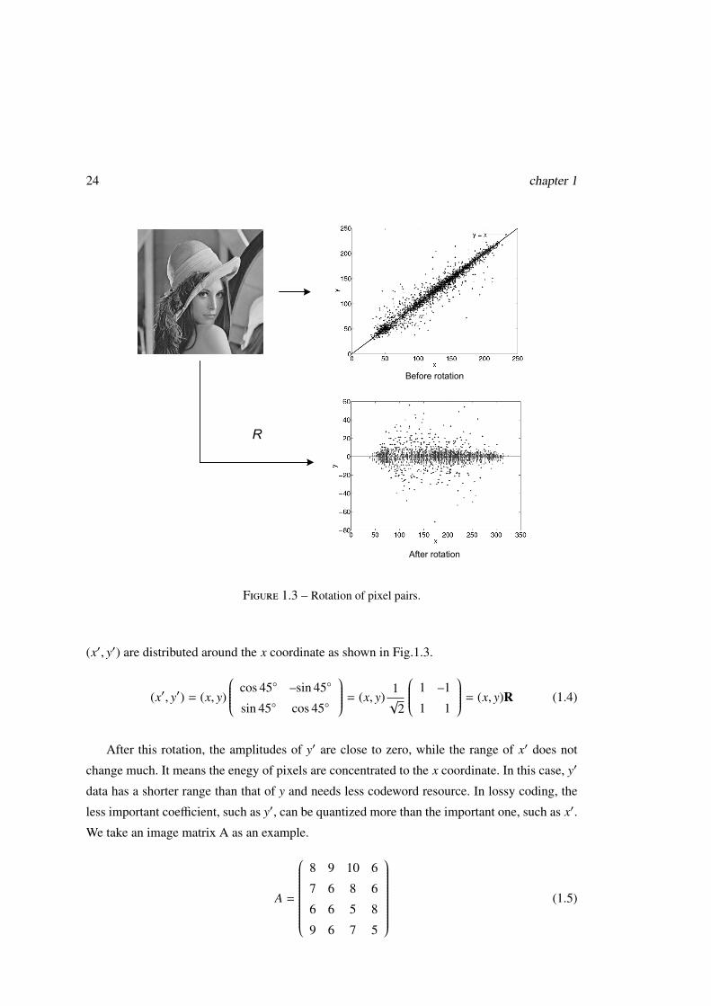
1.1.2 Transform
Transform is another way to convert the pixels (which are correlated) of an image to a more
compact representation where they are decorrelated. One proper method of the transform is the
spatial rotation. Take the image "lena" as an example. We scan the image in raster order and
groupe pairs of adjacent pixels (x, y). Next we plot pairs (x, y) of pixels in two-dimensional
space. For the correlation of adjacent pixels, x and y normally have similar values. Most pairs
(x, y) locate on the line y = x. We rotate the image by multiplying all points with a 45◦ clo-
ckwise rotation matrix (1.4). And then we plot the new (x′, y′) in the space. The rotated pairs
24 chapter 1
Original
imageDecorrelation Quantization
Entropy
coding
Code stream
Entropy
decoding
De-
quantization
Inverse
decorrelation
Recovered
image
encoder
decoder
Xi
...
...
Yi-1Yi-2
Yi-3Yi-4Yi-5Yi-6Yi-7
Yi-8Yi-9Yi-10Yi-11Yi-12 Reference
space
Predicted
pixel
R
Before rotation
After rotation
Figure 1.3 – Rotation of pixel pairs.
(x′, y′) are distributed around the x coordinate as shown in Fig.1.3.
(x′, y′) = (x, y)
cos 45◦ –sin 45◦
sin 45◦ cos 45◦
= (x, y)1√
2
1 –1
1 1
= (x, y)R (1.4)
After this rotation, the amplitudes of y′ are close to zero, while the range of x′ does not
change much. It means the enegy of pixels are concentrated to the x coordinate. In this case, y′
data has a shorter range than that of y and needs less codeword resource. In lossy coding, the
less important coefficient, such as y′, can be quantized more than the important one, such as x′.
We take an image matrix A as an example.
A =
8 9 10 6
7 6 8 6
6 6 5 8
9 6 7 5
(1.5)
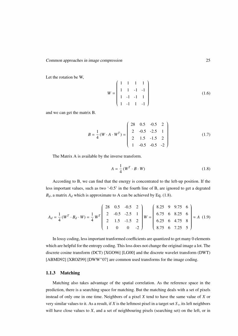
Common approaches in image compression 25
Let the rotation be W,
W =
1 1 1 1
1 1 -1 -1
1 -1 -1 1
1 -1 1 -1
(1.6)
and we can get the matrix B.
B =14
(W · A ·WT ) =
28 0.5 -0.5 2
2 -0.5 -2.5 1
2 1.5 -1.5 2
1 -0.5 -0.5 -2
(1.7)
The Matrix A is available by the inverse transform.
A =14
(WT · B ·W) (1.8)
According to B, we can find that the energy is concentrated to the left-up position. If the
less important values, such as two ‘-0.5’ in the fourth line of B, are ignored to get a degrated
Bd, a matrix Ad which is approximate to A can be achieved by Eq. (1.8).
Ad =14
(WT · Bd ·W) =14
WT
28 0.5 -0.5 2
2 -0.5 -2.5 1
2 1.5 -1.5 2
1 0 0 -2
W =
8.25 9 9.75 6
6.75 6 8.25 6
6.25 6 4.75 8
8.75 6 7.25 5
≈ A (1.9)
In lossy coding, less important tranformed coefficients are quantized to get many 0 elements
which are helpful for the entropy coding. This loss does not change the original image a lot. The
discrete cosine transform (DCT) [XGO96] [LG00] and the discrete wavelet transform (DWT)
[ABMD92] [XROZ99] [DWW+07] are common used transforms for the image coding.
1.1.3 Matching
Matching also takes advantage of the spatial correlation. As the reference space in the
prediction, there is a searching space for matching. But the matching deals with a set of pixels
instead of only one in one time. Neighbors of a pixel X tend to have the same value of X or
very similar values to it. As a result, if X is the leftmost pixel in a target set S t, its left neighbors
will have close values to X, and a set of neighbouring pixels (searching set) on the left, or in
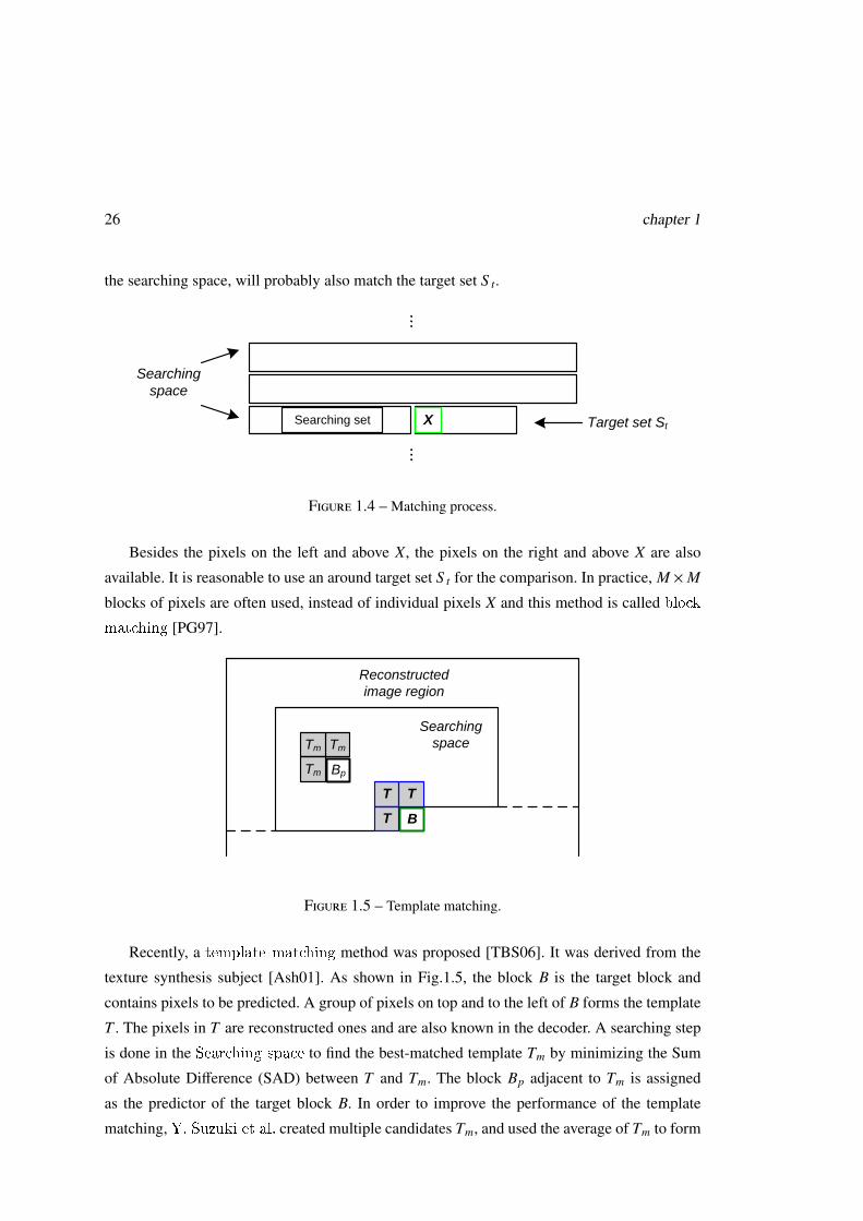
26 chapter 1
the searching space, will probably also match the target set S t.
R
Before rotation
After rotation
X
Searching
space
Searching set Target set St
......
Figure 1.4 – Matching process.
Besides the pixels on the left and above X, the pixels on the right and above X are also
available. It is reasonable to use an around target set S t for the comparison. In practice, M ×M
blocks of pixels are often used, instead of individual pixels X and this method is called block
matching [PG97].
R
Before rotation
After rotation
X
Searching
space
Searching set Target set St
......
Searching
space
Reconstructed
image region
B
TT
T
Tm
Tm
Tm
Bp
Figure 1.5 – Template matching.
Recently, a template matching method was proposed [TBS06]. It was derived from the
texture synthesis subject [Ash01]. As shown in Fig.1.5, the block B is the target block and
contains pixels to be predicted. A group of pixels on top and to the left of B forms the template
T . The pixels in T are reconstructed ones and are also known in the decoder. A searching step
is done in the Searching space to find the best-matched template Tm by minimizing the Sum
of Absolute Difference (SAD) between T and Tm. The block Bp adjacent to Tm is assigned
as the predictor of the target block B. In order to improve the performance of the template
matching, Y. Suzuki et al. created multiple candidates Tm, and used the average of Tm to form
Common approaches in image compression 27
the final predictor, reducing the coding noise [SBT07]. M. Turkan et al. applied the sparse
signal approximation to search a basis function which approximates the known values in T ,
and kept the same basis function and weighting coefficients to estimate the pixels in B [TG10].
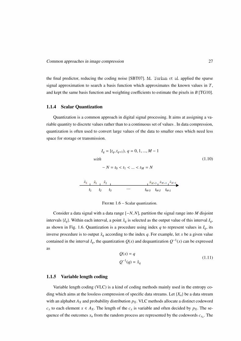
1.1.4 Scalar Quantization
Quantization is a common approach in digital signal processing. It aims at assigning a va-
riable quantity to discrete values rather than to a continuous set of values . In data compression,
quantization is often used to convert large values of the data to smaller ones which need less
space for storage or transmission.
Iq = [tq, tq+1), q = 0, 1, ...,M − 1
with
− N = t0 < t1 < ... < tM = N
(1.10)
HH2
HL2LL2
LH2
LL1 HL1
Tile
HH1LH1
Resolution R2
Resolution R1
Resolution R0
R / L
D
0 LjLj - 1
Dj
Dj - 1
...t1 t2 t3 tM-3 tM-2 tM-1
Figure 1.6 – Scalar quantization.
Consider a data signal with a data range [−N,N], partition the signal range into M disjoint
intervals {Iq}. Within each interval, a point xq is selected as the output value of this interval Iq,
as shown in Fig. 1.6. Quantization is a procedure using index q to represent values in Iq, its
inverse procedure is to output xq according to the index q. For example, let x be a given value
contained in the interval Iq, the quantization Q(x) and dequantization Q−1(x) can be expressed
asQ(x) = q
Q−1(q) = xq
(1.11)
1.1.5 Variable length coding
Variable length coding (VLC) is a kind of coding methods mainly used in the entropy co-
ding which aims at the lossless compression of specific data streams. Let {Xn} be a data stream
with an alphabet AX and probability distribution pX . VLC methods allocate a distinct codeword
cx to each element x ∈ AX . The length of the cx is variable and often decided by pX . The se-
quence of the outcomes xn from the random process are represented by the codewords cxn . The
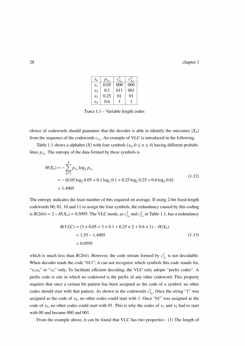
28 chapter 1
xn pxn c1xn
c2xn
x1 0.05 000 000x2 0.1 011 001x3 0.25 01 01x4 0.6 1 1
Table 1.1 – Variable length codes
choice of codewords should guarantee that the decoder is able to identify the outcomes {Xn}
from the sequence of the codewords cxn . An example of VLC is introduced in the following.
Table 1.1 shows a alphabet {X} with four symbols {xn, 0 ≤ n ≤ 4} having different probabi-
lities pxn . The entropy of the data formed by these symbols is
H(Xn) = −
4∑n=1
pxn log2 pxn
= −(0.05 log2 0.05 + 0.1 log2 0.1 + 0.25 log2 0.25 + 0.6 log2 0.6
)= 1.4905
(1.12)
The entropy indicates the least number of bits required on average. If using 2-bit fixed-length
codewords 00, 01, 10 and 11 to assign the four symbols, the redundancy caused by this coding
is R(2bit) = 2−H(Xn) = 0.5095. The VLC mode, as c1xn
and c2xn
in Table 1.1, has a redundancy
R(VLC) = (3 × 0.05 + 3 × 0.1 + 0.25 × 2 + 0.6 × 1) − H(Xn)
= 1.55 − 1.4905
= 0.0595
(1.13)
which is much less than R(2bit). However, the code stream formed by c1xn
is not decodable.
When decoder reads the code “011”, it can not recognize which symbols this code stands for,
“x3x4” or “x2” only. To facilitate efficient decoding, the VLC only adopts “prefix codes”. A
prefix code is one in which no codeword is the prefix of any other codeword. This property
requires that once a certain bit pattern has been assigned as the code of a symbol, no other
codes should start with that pattern. As shown in the codewords c2xn
, Once the string “1” was
assigned as the code of x4, no other codes could start with 1. Once “01” was assigned as the
code of x3, no other codes could start with 01. This is why the codes of x1 and x2 had to start
with 00 and became 000 and 001.
From the example above, it can be found that VLC has two properties : (1) The length of
Still image coding standards 29
the codeword is variable. Assigning short codes to symbols which occur more frequently in
order to reduce required average codeword length ; (2) Codewords have the prefix property.
The classic design of VLC, such as Huffman coding, Golomb coding and Arithmetic coding,
are common methods used in data compression. In practical image coding schemes, the classic
methods are combined with other processes to make up a complex VLC approach. As noted
above, the probability of the symbol is important for the coding ratio. However, the statistic of
probability delays the overall coding and goes against the parallel processing. One solution is to
set context states which identify the most probable symbol. The context state is adaptive during
the coding. This approach can be found in MQ coder [SAT08a] and context-based adaptive
binary arithmetic coding (CABAC) [MSW03].
1.1.6 Conclusion of common methods
Image compression methods are not limited to the approches above. Some methods are
designed for specific type of images or application scenarios. For example, the fractal coding
is suited for images which have parts looking like other ones [WDJ99]. Progressive coding
is adaptive to the storage and transmission capacity for the multiresolution. Modern image
compression schemes have distinctive coding procedures to each other. One scheme can adopt
several coding concepts and use two or more methods for different parts of the image, or in dif-
ferent stages during the procedure. The International Organization for Standardization (ISO)
and International Telecommunication Union (ITU) have announced image compression stan-
dards for practical applications. Four widely used JPEG series will be introduced in Section
1.2.
1.2 Still image coding standards
1.2.1 JPEG
JPEG is the first international compression standard for the continuous tone still images,
both grayscale and color images [Wal92] [CCI92]. It includes two basic compression methods.
A DCT (Discrete cosine transform) based method is specified for lossy compression, and a
predictive method for lossless compression. The lossless mode of JPEG has not been very
successful in the coding efficiency, so ISO has proposed another standard for the lossless image
compression. This standard is known as JPEG-LS and will be introduced in Subsection 1.2.2.
The lossy mode of JPEG has been widely used for natural image coding due to its acceptale
30 chapter 1
Color
Transform8x8 DCT
Uniform Scalar
Quantization
Differential
coding
Zig-zag scan
and RLEVLC
VLC
DC Huffman
tables
AC Huffman
tables
Input
image
DC
ACQuantization
tables
Data
stream
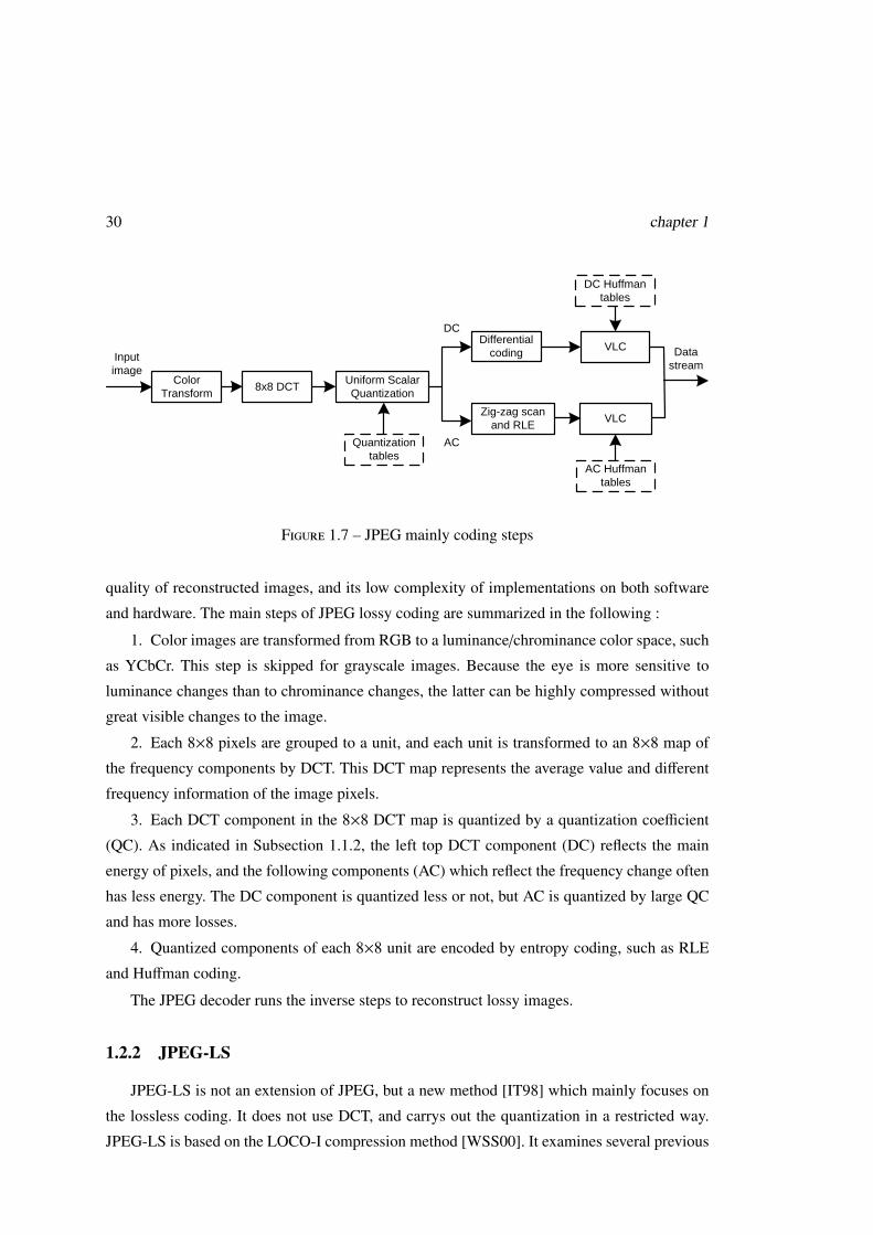
Figure 1.7 – JPEG mainly coding steps
quality of reconstructed images, and its low complexity of implementations on both software
and hardware. The main steps of JPEG lossy coding are summarized in the following :
1. Color images are transformed from RGB to a luminance/chrominance color space, such
as YCbCr. This step is skipped for grayscale images. Because the eye is more sensitive to
luminance changes than to chrominance changes, the latter can be highly compressed without
great visible changes to the image.
2. Each 8×8 pixels are grouped to a unit, and each unit is transformed to an 8×8 map of
the frequency components by DCT. This DCT map represents the average value and different
frequency information of the image pixels.
3. Each DCT component in the 8×8 DCT map is quantized by a quantization coefficient
(QC). As indicated in Subsection 1.1.2, the left top DCT component (DC) reflects the main
energy of pixels, and the following components (AC) which reflect the frequency change often
has less energy. The DC component is quantized less or not, but AC is quantized by large QC
and has more losses.
4. Quantized components of each 8×8 unit are encoded by entropy coding, such as RLE
and Huffman coding.
The JPEG decoder runs the inverse steps to reconstruct lossy images.
1.2.2 JPEG-LS
JPEG-LS is not an extension of JPEG, but a new method [IT98] which mainly focuses on
the lossless coding. It does not use DCT, and carrys out the quantization in a restricted way.
JPEG-LS is based on the LOCO-I compression method [WSS00]. It examines several previous
Still image coding standards 31
R
Before rotation
After rotation
X
Searching
space
Searching set Target set St
......
Searching
space
Reconstructed
image region
B
TT
T
Tm
Tm
Tm
Bp
a
b c d
x y z
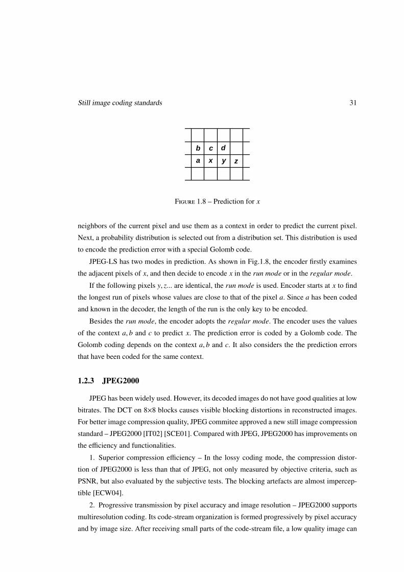
Figure 1.8 – Prediction for x
neighbors of the current pixel and use them as a context in order to predict the current pixel.
Next, a probability distribution is selected out from a distribution set. This distribution is used
to encode the prediction error with a special Golomb code.
JPEG-LS has two modes in prediction. As shown in Fig.1.8, the encoder firstly examines
the adjacent pixels of x, and then decide to encode x in the run mode or in the regular mode.
If the following pixels y, z... are identical, the run mode is used. Encoder starts at x to find
the longest run of pixels whose values are close to that of the pixel a. Since a has been coded
and known in the decoder, the length of the run is the only key to be encoded.
Besides the run mode, the encoder adopts the regular mode. The encoder uses the values
of the context a, b and c to predict x. The prediction error is coded by a Golomb code. The
Golomb coding depends on the context a, b and c. It also considers the the prediction errors
that have been coded for the same context.
1.2.3 JPEG2000
JPEG has been widely used. However, its decoded images do not have good qualities at low
bitrates. The DCT on 8×8 blocks causes visible blocking distortions in reconstructed images.
For better image compression quality, JPEG commitee approved a new still image compression
standard – JPEG2000 [IT02] [SCE01]. Compared with JPEG, JPEG2000 has improvements on
the efficiency and functionalities.
1. Superior compression efficiency – In the lossy coding mode, the compression distor-
tion of JPEG2000 is less than that of JPEG, not only measured by objective criteria, such as
PSNR, but also evaluated by the subjective tests. The blocking artefacts are almost impercep-
tible [ECW04].
2. Progressive transmission by pixel accuracy and image resolution – JPEG2000 supports
multiresolution coding. Its code-stream organization is formed progressively by pixel accuracy
and by image size. After receiving small parts of the code-stream file, a low quality image can
32 chapter 1
HH2
HL2LL2
LH2
LL1 HL1
Tile
HH1LH1
Resolution R2
Resolution R1
Resolution R0
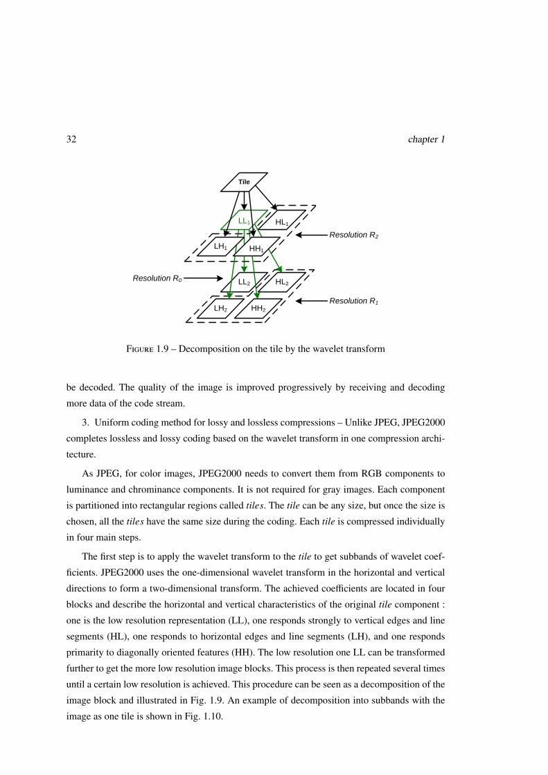
Figure 1.9 – Decomposition on the tile by the wavelet transform
be decoded. The quality of the image is improved progressively by receiving and decoding
more data of the code stream.
3. Uniform coding method for lossy and lossless compressions – Unlike JPEG, JPEG2000
completes lossless and lossy coding based on the wavelet transform in one compression archi-
tecture.
As JPEG, for color images, JPEG2000 needs to convert them from RGB components to
luminance and chrominance components. It is not required for gray images. Each component
is partitioned into rectangular regions called tiles. The tile can be any size, but once the size is
chosen, all the tiles have the same size during the coding. Each tile is compressed individually
in four main steps.
The first step is to apply the wavelet transform to the tile to get subbands of wavelet coef-
ficients. JPEG2000 uses the one-dimensional wavelet transform in the horizontal and vertical
directions to form a two-dimensional transform. The achieved coefficients are located in four
blocks and describe the horizontal and vertical characteristics of the original tile component :
one is the low resolution representation (LL), one responds strongly to vertical edges and line
segments (HL), one responds to horizontal edges and line segments (LH), and one responds
primarity to diagonally oriented features (HH). The low resolution one LL can be transformed
further to get the more low resolution image blocks. This process is then repeated several times
until a certain low resolution is achieved. This procedure can be seen as a decomposition of the
image block and illustrated in Fig. 1.9. An example of decomposition into subbands with the
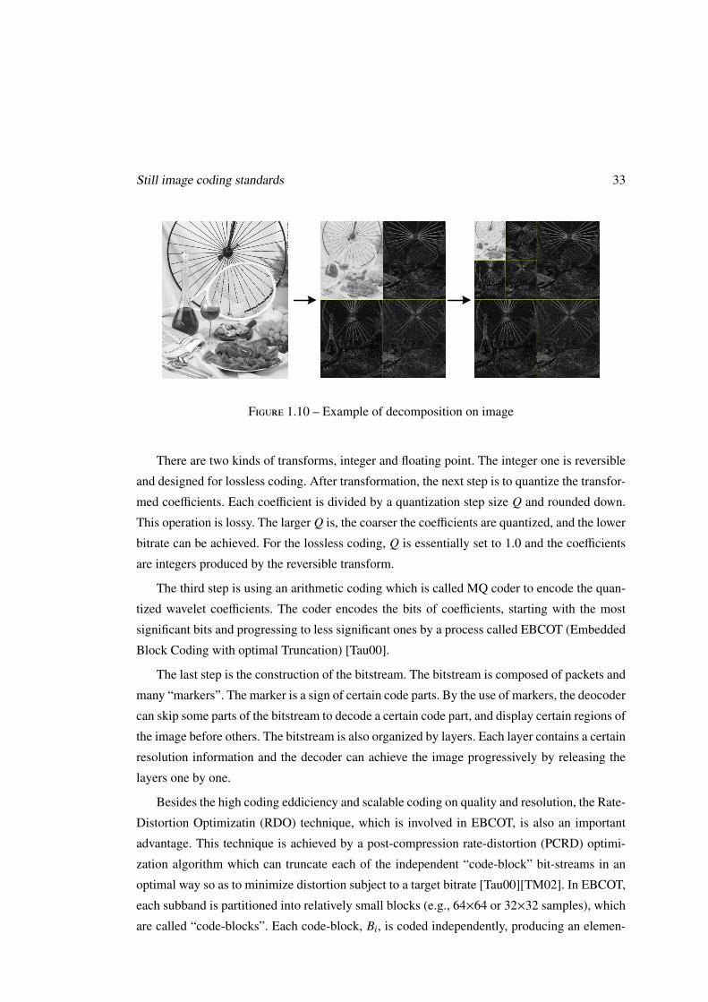
image as one tile is shown in Fig. 1.10.
Still image coding standards 33HH2
HL2LL2
LH2
LL1 HL1
Tile
HH1LH1
Resolution R2
Resolution R1
Resolution R0
Figure 1.10 – Example of decomposition on image
There are two kinds of transforms, integer and floating point. The integer one is reversible
and designed for lossless coding. After transformation, the next step is to quantize the transfor-
med coefficients. Each coefficient is divided by a quantization step size Q and rounded down.
This operation is lossy. The larger Q is, the coarser the coefficients are quantized, and the lower
bitrate can be achieved. For the lossless coding, Q is essentially set to 1.0 and the coefficients
are integers produced by the reversible transform.
The third step is using an arithmetic coding which is called MQ coder to encode the quan-
tized wavelet coefficients. The coder encodes the bits of coefficients, starting with the most
significant bits and progressing to less significant ones by a process called EBCOT (Embedded
Block Coding with optimal Truncation) [Tau00].
The last step is the construction of the bitstream. The bitstream is composed of packets and
many “markers”. The marker is a sign of certain code parts. By the use of markers, the deocoder
can skip some parts of the bitstream to decode a certain code part, and display certain regions of
the image before others. The bitstream is also organized by layers. Each layer contains a certain
resolution information and the decoder can achieve the image progressively by releasing the
layers one by one.
Besides the high coding eddiciency and scalable coding on quality and resolution, the Rate-
Distortion Optimizatin (RDO) technique, which is involved in EBCOT, is also an important
advantage. This technique is achieved by a post-compression rate-distortion (PCRD) optimi-
zation algorithm which can truncate each of the independent “code-block” bit-streams in an
optimal way so as to minimize distortion subject to a target bitrate [Tau00][TM02]. In EBCOT,
each subband is partitioned into relatively small blocks (e.g., 64×64 or 32×32 samples), which
are called “code-blocks”. Each code-block, Bi, is coded independently, producing an elemen-
34 chapter 1
tary bitstream ci. It is assumed that the overrall distortion of the reconstructed image can be
represented as a sum of distortions from each code-block. Let Di denote the distortion contri-
buted by the block Bi, if its elementary bitstream is truncated to the length Li, the overall length
of the final compressed bitstream is constrained as Lmax, the selection of the set of trunction
points {zi} should have ∑i
L(zi)i ≤ Lmax (1.14)
and can minimize the overall distortion D.
D =∑
i
D(zi)i (1.15)
In order to combine Eq.(1.14) and Eq.(1.15), a quantity λ is involved. Let {zi,λ} be the set of
truncation points which minimizes
D(λ) + λL(λ) =∑
i
(D(zi,λ)
i + λL(zi,λ)i
)(1.16)
Where λ > 0. The truncation points {zi,λ} are optimal, when the distortion D cannot be further
reduced. Thus, it is desired to find a value of λ such that the truncation points {zi,λ} which can
minimize Eq. (1.16) yield L(λ) = Lmax. Since the set of available truncation points is discrete,
the suitable λ could not be found to make L(λ) be exactly equal to Lmax. Nevertheless, the
code-blocks are relatively small and there are typically many truncation points to find λ to
meet L(λ) ≤ Lmax. PCRD does not try to find the optimal truncation points zopt of Eq.(1.16)
directly, but focuses on(D(zi,λ)
i + λL(zi,λ)i
)for each code-block Bi respectively. For a given λ > 0 :
1. Initialize zopt = 0.
2. For j = 1, 2, ..., set ∆L = L ji − Lzopt
i , and ∆D = Dzopti − D j
i . ∆L is the increment of the
length, and ∆D is the decrement of the distortion if zopt is replaced by j. If ∆D/∆L > λ, replace
zopt by j. This step guarantees that D(zopt)i + λL(zopt)
i ≤ D(z)i + λL(z)
i for all z ≤ t.
3. Set zi,λ = zopt.
Because the number of code-blocks may be very large, and the searching for zopt needs
to be executed under many different λ, a subset Hi which contains feasible truncation points
should be found to reduce unnecessary computation.
Fig. 1.11 illustrates an example of rate distortion curve. It can be noticed that the distortion
D dicreases while the bitrate R increases (the length of the bit-stream L will replace R in the
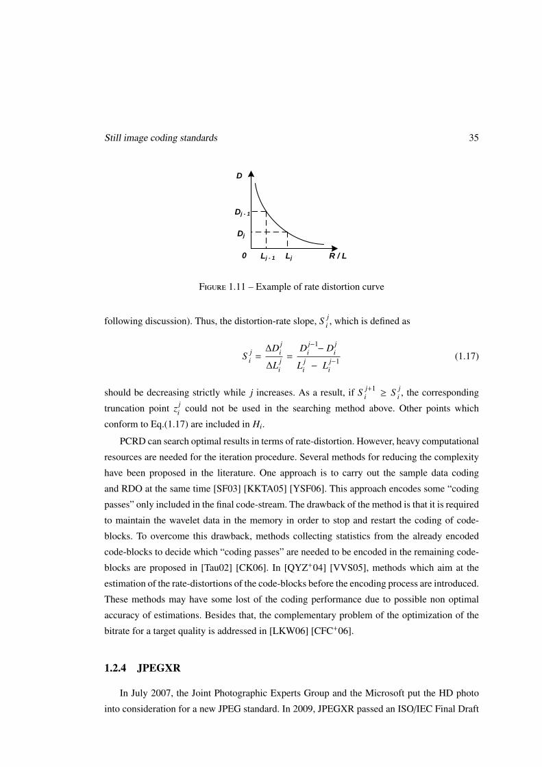
Still image coding standards 35
HH2
HL2LL2
LH2
LL1 HL1
Tile
HH1LH1
Resolution R2
Resolution R1
Resolution R0
R / L
D
0 LjLj - 1
Dj
Dj - 1
Figure 1.11 – Example of rate distortion curve
following discussion). Thus, the distortion-rate slope, S ji , which is defined as
S ji =
∆D ji
∆L ji
=D j−1
i − D ji
L ji − L j−1
i
(1.17)
should be decreasing strictly while j increases. As a result, if S j+1i ≥ S j
i , the corresponding
truncation point z ji could not be used in the searching method above. Other points which
conform to Eq.(1.17) are included in Hi.
PCRD can search optimal results in terms of rate-distortion. However, heavy computational
resources are needed for the iteration procedure. Several methods for reducing the complexity
have been proposed in the literature. One approach is to carry out the sample data coding
and RDO at the same time [SF03] [KKTA05] [YSF06]. This approach encodes some “coding
passes” only included in the final code-stream. The drawback of the method is that it is required
to maintain the wavelet data in the memory in order to stop and restart the coding of code-
blocks. To overcome this drawback, methods collecting statistics from the already encoded
code-blocks to decide which “coding passes” are needed to be encoded in the remaining code-
blocks are proposed in [Tau02] [CK06]. In [QYZ+04] [VVS05], methods which aim at the
estimation of the rate-distortions of the code-blocks before the encoding process are introduced.
These methods may have some lost of the coding performance due to possible non optimal
accuracy of estimations. Besides that, the complementary problem of the optimization of the
bitrate for a target quality is addressed in [LKW06] [CFC+06].
1.2.4 JPEGXR
In July 2007, the Joint Photographic Experts Group and the Microsoft put the HD photo
into consideration for a new JPEG standard. In 2009, JPEGXR passed an ISO/IEC Final Draft
36 chapter 1
International Standard (FDIS) ballot to be a new still image compression standard and file
format for continuous tone photographic images [ISO09]. JPEGXR is based on the technology
developed by Microsoft under the name HD Photo[STZ+07].
Compared with JPEG, JPEGXR also shows a better quality at an equivalent compression
ratio. Its compression efficiency is close to, but not exceeds that of JPEG2000 [DSOD+07].
Although JPEG2000 has provided high coding ratios, it is not put into wide application for
the reason of the high computation complexity, especially caused by EBCOT. JPEGXR was
proposed to offer a low complexity coding solution. It has same capabilities as JPEG2000,
such as the same processing steps for both lossless and lossy coding, and coding images by
segmented tile regions.
JPEGXR uses an integer transform adopting a lifting scheme [TSS+08]. This transform is
close to a 4×4 DCT but is lossless. JPEGXR allows an optional overlap step. This step operates
on 4×4 blocks which are offset by 2 samples in each direction from the 4×4 core transform
blocks. Its purpose is to improve compression capability and reduce block-boundary artifacts
at low bitrates. At high bitrates, when the block-boundary artifacts are not obvious, this overlap
step is skipped for reducing the encoding and decoding time.
JPEGXR format (.JXR) is popularized mainly by Microsoft, it is supported in Adobe Flash
Player 11, Windows Imaging Component, Windows operating systems, such as Windows Vista,
Windows 7 and 8, Internet Explorer from 9 to 11.
1.3 Nonstandard still image coding methods
Besides the standards, there are many other image coding methods. Some of them deal
with lossy compression trying to achieve high qualities of decoded images as far as possible
[ZZX14] ; some concentrate on the bitrate only for lossless coding [WSLY09], and also one
general coder performing lossless and lossy coding is desirable [PINS04]. Most contributions
are published in literature, but a few of them provide reference programmes. In this section
we present two efficient image coding methods which have been tested by researchers and
practitioners.
1.3.1 CALIC
The name “CALIC” stands for Context-based, Adaptive, Lossless Image Compression
[WM96] [WM97]. It is one of the best performing practical and general purpose lossless image
coding techniques.
Nonstandard still image coding methods 37
Binary
mode ?
yy
Gap
PredictorContext Formation
& Quantization
y yp
Two Row Buffer
Binary
Context
Formation
Bias
Cancellation
Binary
Context
Formation
Entropy
Codingy
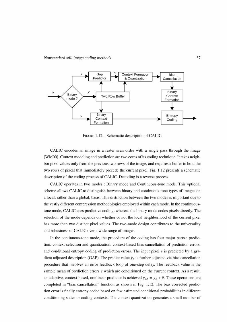
Figure 1.12 – Schematic description of CALIC
CALIC encodes an image in a raster scan order with a single pass through the image
[WM00]. Context modeling and prediction are two cores of its coding technique. It takes neigh-
bor pixel values only from the previous two rows of the image, and requires a buffer to hold the
two rows of pixels that immediately precede the current pixel. Fig. 1.12 presents a schematic
description of the coding process of CALIC. Decoding is a reverse process.
CALIC operates in two modes : Binary mode and Continuous-tone mode. This optional
scheme allows CALIC to distinguish between binary and continuous-tone types of images on
a local, rather than a global, basis. This distinction between the two modes is important due to
the vastly different compression methodologies employed within each mode. In the continuous-
tone mode, CALIC uses predictive coding, whereas the binary mode codes pixels directly. The
selection of the mode depends on whether or not the local neighborhood of the current pixel
has more than two distinct pixel values. The two-mode design contributes to the universality
and robustness of CALIC over a wide range of images.
In the continuous-tone mode, the procedure of the coding has four major parts : predic-
tion, context selection and quantization, context-based bias cancellation of prediction errors,
and conditional entropy coding of prediction errors. The input pixel y is predicted by a gra-
dient adjusted description (GAP). The predict value yp is further adjusted via bias cancellation
procedure that involves an error feedback loop of one-step delay. The feedback value is the
sample mean of prediction errors e which are conditioned on the current context. As a result,
an adaptive, context-based, nonlinear predictor is achieved yap = yp + e. These operations are
completed in “bias cancellation” function as shown in Fig. 1.12. The bias corrected predic-
tion error is finally entropy coded based on few estimated conditional probabilities in different
conditioning states or coding contexts. The context quantization generates a small number of
38 chapter 1
Binary
mode ?
yy
Gap
PredictorContext Formation
& Quantization
y yp
Two Row Buffer
Binary
Context
Formation
Bias
Cancellation
Binary
Context
Formation
Entropy
Codingy
y1 y
y2y3 y4
y5
y6y7
y8
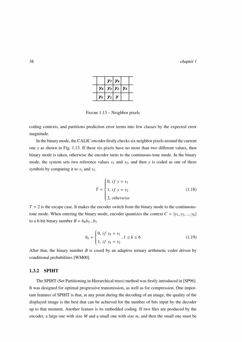
Figure 1.13 – Neighbor pixels
coding contexts, and partitions prediction error terms into few classes by the expected error
magnitude.
In the binary mode, the CALIC encoder firstly checks six neighbor pixels around the current
one y as shown in Fig. 1.13. If these six pixels have no more than two different values, then
binary mode is taken, otherwise the encoder turns to the continuous-tone mode. In the binary
mode, the system sets two reference values s1 and s2, and then y is coded as one of three
symbols by comparing it to s1 and s2.
T =
0, i f y = s1
1, i f y = s2
2, otherwise
(1.18)
T = 2 is the escape case. It makes the encoder switch from the binary mode to the continuous-
tone mode. When entering the binary mode, encoder quantizes the context C = {y1, y2, ..., y6}
to a 6-bit binary number B = b6b5...b1
bk =
0, i f yk = s1
1, i f yk = s2
, 1 ≤ k ≤ 6 (1.19)
After that, the binary number B is cosed by an adaptive ternary arithmetic coder driven by
conditional probabilities [WM00].
1.3.2 SPIHT
The SPIHT (Set Partitioning in Hierarchical trees) method was firstly introduced in [SP96].
It was designed for optimal progressive transmission, as well as for compression. One impor-
tant features of SPIHT is that, at any point during the decoding of an image, the quality of the
displayed image is the best that can be achieved for the number of bits input by the decoder
up to that moment. Another feature is its embedded coding. If two files are produced by the
encoder, a large one with size M and a small one with size m, and then the small one must be
Nonstandard still image coding methods 39
k 1 2 3 4 5 6sign s s s s s s14 1 1 0 0 0 013 a b 1 1 0 012 c d e f 1 1...
......
......
......
0 h i g k l m
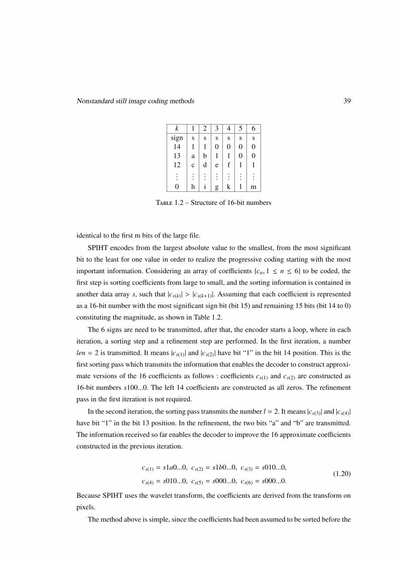
Table 1.2 – Structure of 16-bit numbers
identical to the first m bits of the large file.
SPIHT encodes from the largest absolute value to the smallest, from the most significant
bit to the least for one value in order to realize the progressive coding starting with the most
important information. Considering an array of coefficients {cn, 1 ≤ n ≤ 6} to be coded, the
first step is sorting coefficients from large to small, and the sorting information is contained in
another data array s, such that |cs(k)| > |cs(k+1)|. Assuming that each coefficient is represented
as a 16-bit number with the most significant sign bit (bit 15) and remaining 15 bits (bit 14 to 0)
constituting the magnitude, as shown in Table 1.2.
The 6 signs are need to be transmitted, after that, the encoder starts a loop, where in each
iteration, a sorting step and a refinement step are performed. In the first iteration, a number
len = 2 is transmitted. It means |cs(1)| and |cs(2)| have bit “1” in the bit 14 position. This is the
first sorting pass which transmits the information that enables the decoder to construct approxi-
mate versions of the 16 coefficients as follows : coefficients cs(1) and cs(2) are constructed as
16-bit numbers s100...0. The left 14 coefficients are constructed as all zeros. The refinement
pass in the first iteration is not required.
In the second iteration, the sorting pass transmits the number l = 2. It means |cs(3)| and |cs(4)|
have bit “1” in the bit 13 position. In the refinement, the two bits “a” and “b” are transmitted.
The information received so far enables the decoder to improve the 16 approximate coefficients
constructed in the previous iteration.
cs(1) = s1a0...0, cs(2) = s1b0...0, cs(3) = s010...0,
cs(4) = s010...0, cs(5) = s000...0, cs(6) = s000...0.(1.20)
Because SPIHT uses the wavelet transform, the coefficients are derived from the transform on
pixels.
The method above is simple, since the coefficients had been assumed to be sorted before the
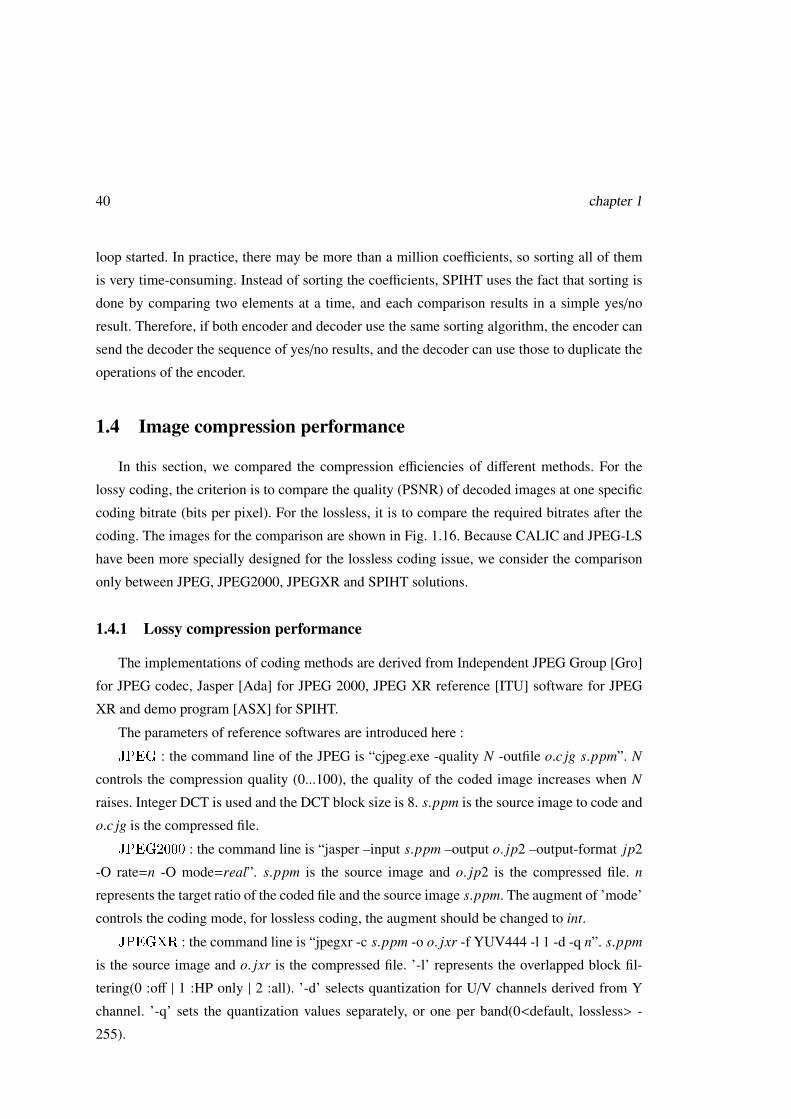
40 chapter 1
loop started. In practice, there may be more than a million coefficients, so sorting all of them
is very time-consuming. Instead of sorting the coefficients, SPIHT uses the fact that sorting is
done by comparing two elements at a time, and each comparison results in a simple yes/no
result. Therefore, if both encoder and decoder use the same sorting algorithm, the encoder can
send the decoder the sequence of yes/no results, and the decoder can use those to duplicate the
operations of the encoder.
1.4 Image compression performance
In this section, we compared the compression efficiencies of different methods. For the
lossy coding, the criterion is to compare the quality (PSNR) of decoded images at one specific
coding bitrate (bits per pixel). For the lossless, it is to compare the required bitrates after the
coding. The images for the comparison are shown in Fig. 1.16. Because CALIC and JPEG-LS
have been more specially designed for the lossless coding issue, we consider the comparison
only between JPEG, JPEG2000, JPEGXR and SPIHT solutions.
1.4.1 Lossy compression performance
The implementations of coding methods are derived from Independent JPEG Group [Gro]
for JPEG codec, Jasper [Ada] for JPEG 2000, JPEG XR reference [ITU] software for JPEG
XR and demo program [ASX] for SPIHT.
The parameters of reference softwares are introduced here :
JPEG : the command line of the JPEG is “cjpeg.exe -quality N -outfile o.c jg s.ppm”. N
controls the compression quality (0...100), the quality of the coded image increases when N
raises. Integer DCT is used and the DCT block size is 8. s.ppm is the source image to code and
o.c jg is the compressed file.
JPEG2000 : the command line is “jasper –input s.ppm –output o. jp2 –output-format jp2
-O rate=n -O mode=real”. s.ppm is the source image and o. jp2 is the compressed file. n
represents the target ratio of the coded file and the source image s.ppm. The augment of ’mode’
controls the coding mode, for lossless coding, the augment should be changed to int.
JPEGXR : the command line is “jpegxr -c s.ppm -o o. jxr -f YUV444 -l 1 -d -q n”. s.ppm
is the source image and o. jxr is the compressed file. ’-l’ represents the overlapped block fil-
tering(0 :off | 1 :HP only | 2 :all). ’-d’ selects quantization for U/V channels derived from Y
channel. ’-q’ sets the quantization values separately, or one per band(0<default, lossless> -
255).
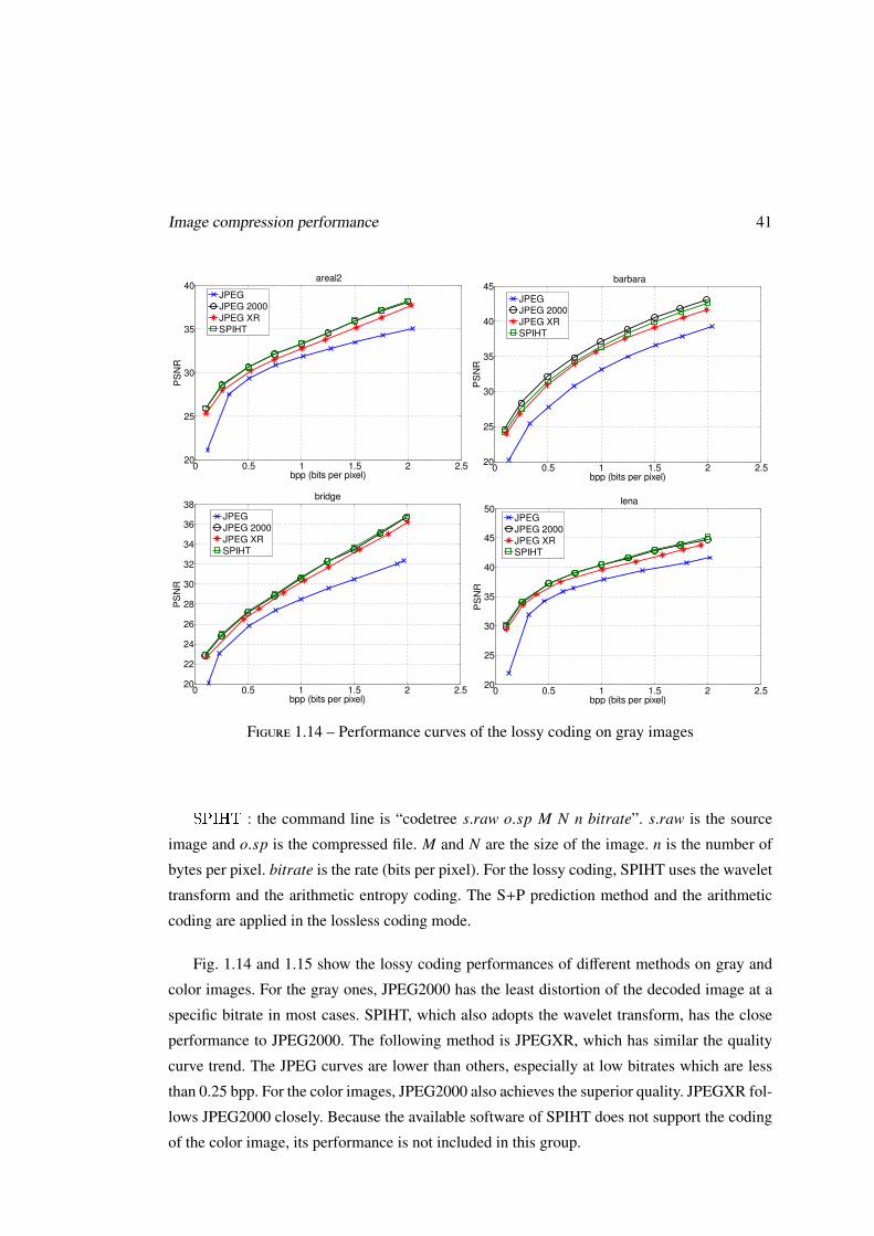
Image compression performance 41
0 0.5 1 1.5 2 2.520
25
30
35
40
bpp (bits per pixel)
PS
NR
areal2
JPEG
JPEG 2000
JPEG XR
SPIHT
0 0.5 1 1.5 2 2.520
25
30
35
40
45
bpp (bits per pixel)
PS
NR
barbara
JPEGJPEG 2000
JPEG XRSPIHT
0 0.5 1 1.5 2 2.520
25
30
35
40
bpp (bits per pixel)
PS
NR
areal2
JPEG
JPEG 2000
JPEG XR
SPIHT
0 0.5 1 1.5 2 2.520
25
30
35
40
45
bpp (bits per pixel)P
SN
R
barbara
JPEGJPEG 2000
JPEG XRSPIHT
0 0.5 1 1.5 2 2.520
22
24
26
28
30
32
34
36
38
bpp (bits per pixel)
PS
NR
bridge
JPEG
JPEG 2000
JPEG XR
SPIHT
0 0.5 1 1.5 2 2.520
25
30
35
40
45
50
bpp (bits per pixel)
PS
NR
lena
JPEG
JPEG 2000JPEG XR
SPIHT
0 0.5 1 1.5 2 2.520
22
24
26
28
30
32
34
36
38
bpp (bits per pixel)P
SN
R
bridge
JPEG
JPEG 2000
JPEG XR
SPIHT
0 0.5 1 1.5 2 2.520
25
30
35
40
45
50
bpp (bits per pixel)
PS
NR
lena
JPEG
JPEG 2000JPEG XR
SPIHT
Figure 1.14 – Performance curves of the lossy coding on gray images
SPIHT : the command line is “codetree s.raw o.sp M N n bitrate”. s.raw is the source
image and o.sp is the compressed file. M and N are the size of the image. n is the number of
bytes per pixel. bitrate is the rate (bits per pixel). For the lossy coding, SPIHT uses the wavelet
transform and the arithmetic entropy coding. The S+P prediction method and the arithmetic
coding are applied in the lossless coding mode.
Fig. 1.14 and 1.15 show the lossy coding performances of different methods on gray and
color images. For the gray ones, JPEG2000 has the least distortion of the decoded image at a
specific bitrate in most cases. SPIHT, which also adopts the wavelet transform, has the close
performance to JPEG2000. The following method is JPEGXR, which has similar the quality
curve trend. The JPEG curves are lower than others, especially at low bitrates which are less
than 0.25 bpp. For the color images, JPEG2000 also achieves the superior quality. JPEGXR fol-
lows JPEG2000 closely. Because the available software of SPIHT does not support the coding
of the color image, its performance is not included in this group.
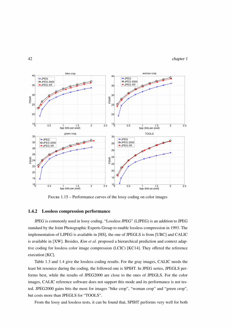
42 chapter 1
0 0.5 1 1.5 2 2.515
20
25
30
35
40
bpp (bits per pixel)
PS
NR
bike crop
JPEG
JPEG 2000
JPEG XR
0 0.5 1 1.5 2 2.515
20
25
30
35
40
bpp (bits per pixel)
PS
NR
woman crop
JPEG
JPEG 2000JPEG XR
0 0.5 1 1.5 2 2.515
20
25
30
35
40
bpp (bits per pixel)
PS
NR
bike crop
JPEG
JPEG 2000
JPEG XR
0 0.5 1 1.5 2 2.515
20
25
30
35
40
bpp (bits per pixel)
PS
NR
woman crop
JPEG
JPEG 2000JPEG XR
0 0.5 1 1.5 2 2.516
18
20
22
24
26
28
30
32
bpp (bits per pixel)
PS
NR
green crop
JPEG
JPEG 2000
JPEG XR
0 0.5 1 1.5 2 2.516
18
20
22
24
26
28
30
bpp (bits pe pixel)
PS
NR
TOOLS
JPEGJPEG 2000
JPEG XR
0 0.5 1 1.5 2 2.516
18
20
22
24
26
28
30
32
bpp (bits per pixel)
PS
NR
green crop
JPEG
JPEG 2000
JPEG XR
0 0.5 1 1.5 2 2.516
18
20
22
24
26
28
30
bpp (bits pe pixel)
PS
NR
TOOLS
JPEGJPEG 2000
JPEG XR
Figure 1.15 – Performance curves of the lossy coding on color images
1.4.2 Lossless compression performance
JPEG is commonly used in lossy coding. “Lossless JPEG” (LJPEG) is an addition to JPEG
standard by the Joint Photographic Experts Group to enable lossless compression in 1993. The
implementation of LJPEG is available in [HS], the one of JPEGLS is from [UBC] and CALIC
is available in [XW]. Besides, Kim et al. proposed a hierarchical prediction and context adap-
tive coding for lossless color image compression (LCIC) [KC14]. They offered the reference
execution [KC].
Table 1.3 and 1.4 give the lossless coding results. For the gray images, CALIC needs the
least bit resource during the coding, the followed one is SPIHT. In JPEG series, JPEGLS per-
forms best, while the results of JPEG2000 are close to the ones of JPEGLS. For the color
images, CALIC reference software does not support this mode and its performance is not tes-
ted. JPEG2000 gains bits the most for images “bike crop”, “woman crop” and “green crop”,
but costs more than JPEGLS for “TOOLS”.
From the lossy and lossless tests, it can be found that, SPIHT performs very well for both
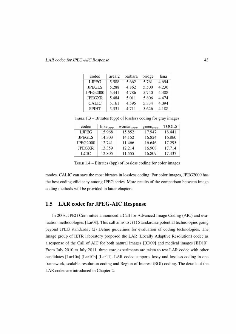
LAR codec for JPEG-AIC Response 43
codec areal2 barbara bridge lenaLJPEG 5.588 5.662 5.761 4.694
JPEGLS 5.288 4.862 5.500 4.236JPEG2000 5.441 4.786 5.740 4.308JPEGXR 5.484 5.011 5.806 4.474CALIC 5.161 4.595 5.334 4.094SPIHT 5.331 4.711 5.626 4.188
Table 1.3 – Bitrates (bpp) of lossless coding for gray images
codec bikecrop womancrop greencrop TOOLSLJPEG 15.968 15.852 17.947 18.441
JPEGLS 14.303 14.152 16.824 16.860JPEG2000 12.741 11.466 16.646 17.295JPEGXR 13.359 12.214 16.908 17.714
LCIC 12.805 11.555 16.809 17.437
Table 1.4 – Bitrates (bpp) of lossless coding for color images
modes. CALIC can save the most bitrates in lossless coding. For color images, JPEG2000 has
the best coding efficiency among JPEG series. More results of the comparison between image
coding methods will be provided in latter chapters.
1.5 LAR codec for JPEG-AIC Response
In 2008, JPEG Committee announced a Call for Advanced Image Coding (AIC) and eva-
luation methodologies [Lar08]. This call aims to : (1) Standardize potential technologies going
beyond JPEG standards ; (2) Define guidelines for evaluation of coding technologies. The
Image group of IETR laboratory proposed the LAR (Locally Adaptive Resolution) codec as
a response of the Call of AIC for both natural images [BD09] and medical images [BD10].
From July 2010 to July 2011, three core experiments are taken to test LAR codec with other
candidates [Lar10a] [Lar10b] [Lar11]. LAR codec supports lossy and lossless coding in one
framework, scalable resolution coding and Region of Interest (ROI) coding. The details of the
LAR codec are introduced in Chapter 2.
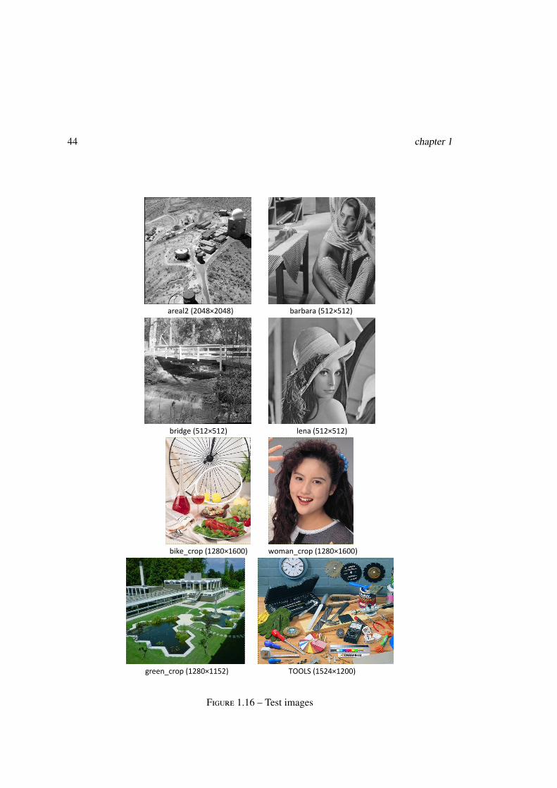
44 chapter 1
areal2 (2048×2048) barbara (512×512)
bridge (512×512) lena (512×512)
bike_crop (1280×1600) woman_crop (1280×1600)
green_crop (1280×1152) TOOLS (1524×1200)
Figure 1.16 – Test images
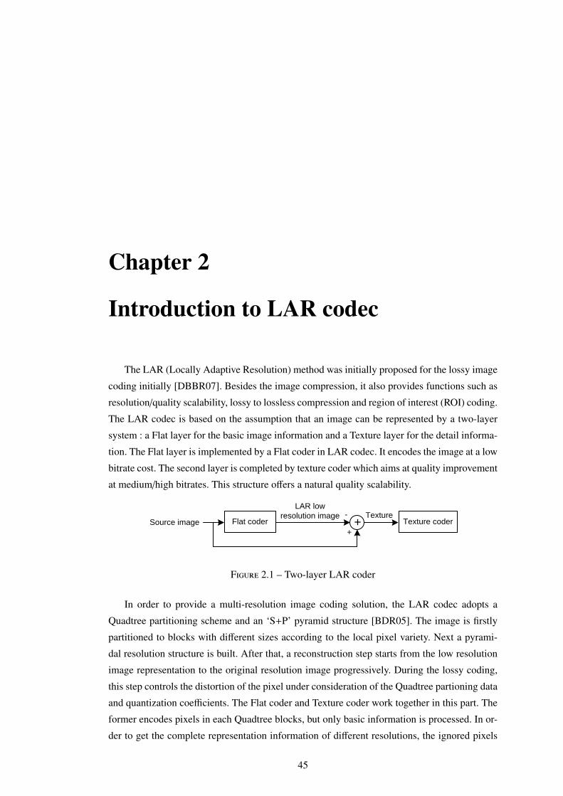
Chapter 2
Introduction to LAR codec
The LAR (Locally Adaptive Resolution) method was initially proposed for the lossy image
coding initially [DBBR07]. Besides the image compression, it also provides functions such as
resolution/quality scalability, lossy to lossless compression and region of interest (ROI) coding.
The LAR codec is based on the assumption that an image can be represented by a two-layer
system : a Flat layer for the basic image information and a Texture layer for the detail informa-
tion. The Flat layer is implemented by a Flat coder in LAR codec. It encodes the image at a low
bitrate cost. The second layer is completed by texture coder which aims at quality improvement
at medium/high bitrates. This structure offers a natural quality scalability.
Source image Flat coder
LAR low
resolution image+
+
- TextureTexture coder
Figure 2.1 – Two-layer LAR coder
In order to provide a multi-resolution image coding solution, the LAR codec adopts a
Quadtree partitioning scheme and an ‘S+P’ pyramid structure [BDR05]. The image is firstly
partitioned to blocks with different sizes according to the local pixel variety. Next a pyrami-
dal resolution structure is built. After that, a reconstruction step starts from the low resolution
image representation to the original resolution image progressively. During the lossy coding,
this step controls the distortion of the pixel under consideration of the Quadtree partioning data
and quantization coefficients. The Flat coder and Texture coder work together in this part. The
former encodes pixels in each Quadtree blocks, but only basic information is processed. In or-
der to get the complete representation information of different resolutions, the ignored pixels
45
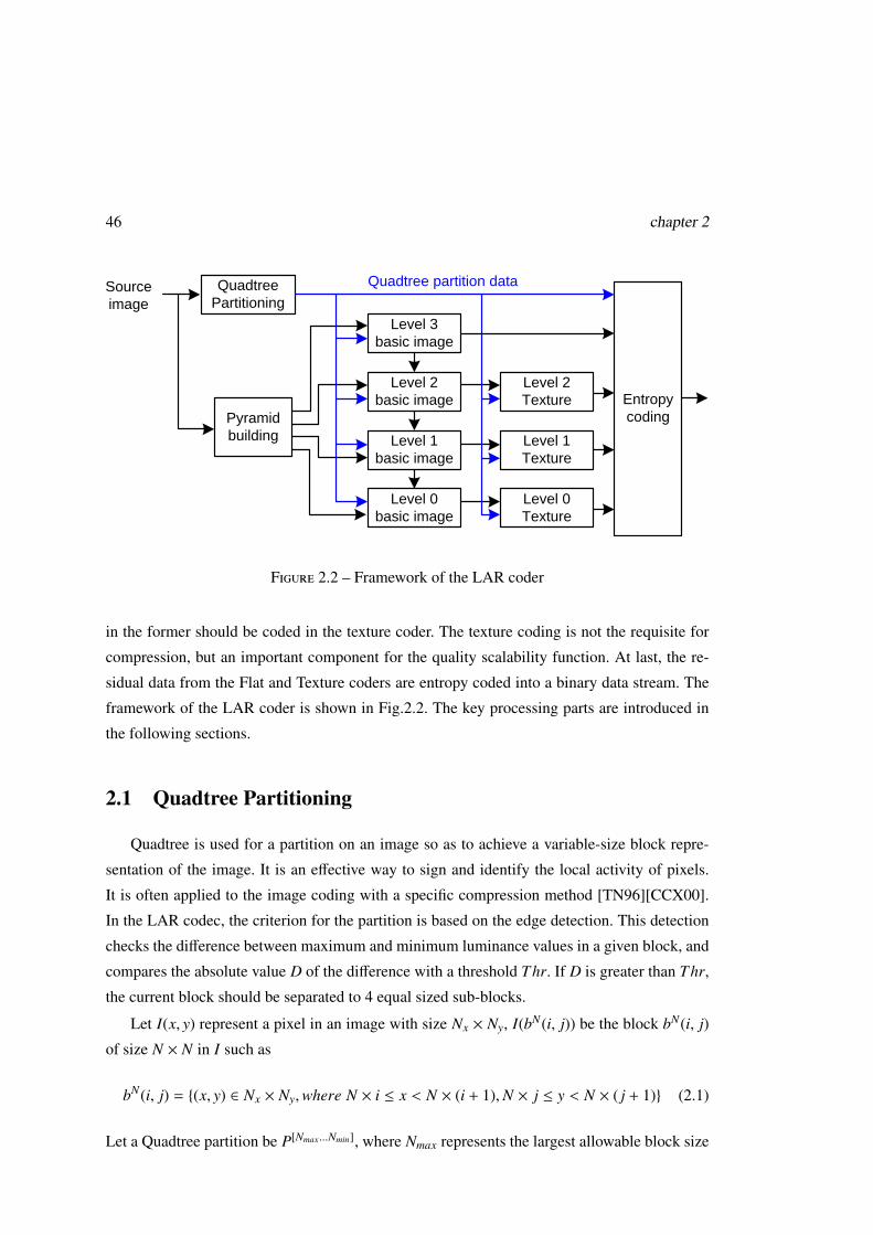
46 chapter 2
Source image Flat coder
LAR low
resolution image+
+
- TextureTexture coder
Source
image
Quadtree
Partitioning
Pyramid
building
Level 3
basic image
Level 2
basic image
Level 1
basic image
Level 0
basic image
Level 2
Texture
Level 1
Texture
Level 0
Texture
Entropy
coding
Quadtree partition data
Figure 2.2 – Framework of the LAR coder
in the former should be coded in the texture coder. The texture coding is not the requisite for
compression, but an important component for the quality scalability function. At last, the re-
sidual data from the Flat and Texture coders are entropy coded into a binary data stream. The
framework of the LAR coder is shown in Fig.2.2. The key processing parts are introduced in
the following sections.
2.1 Quadtree Partitioning
Quadtree is used for a partition on an image so as to achieve a variable-size block repre-
sentation of the image. It is an effective way to sign and identify the local activity of pixels.
It is often applied to the image coding with a specific compression method [TN96][CCX00].
In the LAR codec, the criterion for the partition is based on the edge detection. This detection
checks the difference between maximum and minimum luminance values in a given block, and
compares the absolute value D of the difference with a threshold Thr. If D is greater than Thr,
the current block should be separated to 4 equal sized sub-blocks.
Let I(x, y) represent a pixel in an image with size Nx × Ny, I(bN(i, j)) be the block bN(i, j)
of size N × N in I such as
bN(i, j) = {(x, y) ∈ Nx × Ny,where N × i ≤ x < N × (i + 1),N × j ≤ y < N × ( j + 1)} (2.1)
Let a Quadtree partition be P[Nmax...Nmin], where Nmax represents the largest allowable block size
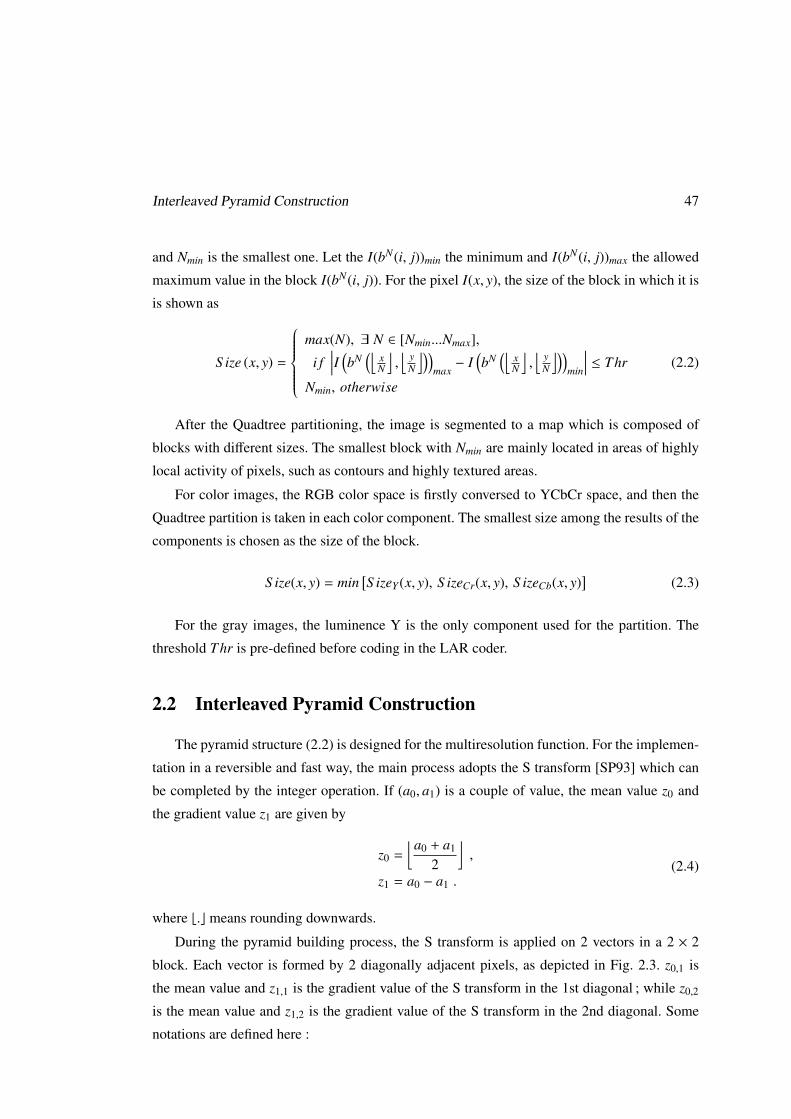
Interleaved Pyramid Construction 47
and Nmin is the smallest one. Let the I(bN(i, j))min the minimum and I(bN(i, j))max the allowed
maximum value in the block I(bN(i, j)). For the pixel I(x, y), the size of the block in which it is
is shown as
S ize (x, y) =
max(N), ∃ N ∈ [Nmin...Nmax],
i f∣∣∣∣I (
bN(⌊
xN
⌋,⌊
yN
⌋))max− I
(bN
(⌊xN
⌋,⌊
yN
⌋))min
∣∣∣∣ ≤ Thr
Nmin, otherwise
(2.2)
After the Quadtree partitioning, the image is segmented to a map which is composed of
blocks with different sizes. The smallest block with Nmin are mainly located in areas of highly
local activity of pixels, such as contours and highly textured areas.
For color images, the RGB color space is firstly conversed to YCbCr space, and then the
Quadtree partition is taken in each color component. The smallest size among the results of the
components is chosen as the size of the block.
S ize(x, y) = min[S izeY (x, y), S izeCr(x, y), S izeCb(x, y)
](2.3)
For the gray images, the luminence Y is the only component used for the partition. The
threshold Thr is pre-defined before coding in the LAR coder.
2.2 Interleaved Pyramid Construction
The pyramid structure (2.2) is designed for the multiresolution function. For the implemen-
tation in a reversible and fast way, the main process adopts the S transform [SP93] which can
be completed by the integer operation. If (a0, a1) is a couple of value, the mean value z0 and
the gradient value z1 are given by
z0 =
⌊a0 + a1
2
⌋,
z1 = a0 − a1 .(2.4)
where b.c means rounding downwards.
During the pyramid building process, the S transform is applied on 2 vectors in a 2 × 2
block. Each vector is formed by 2 diagonally adjacent pixels, as depicted in Fig. 2.3. z0,1 is
the mean value and z1,1 is the gradient value of the S transform in the 1st diagonal ; while z0,2
is the mean value and z1,2 is the gradient value of the S transform in the 2nd diagonal. Some
notations are defined here :
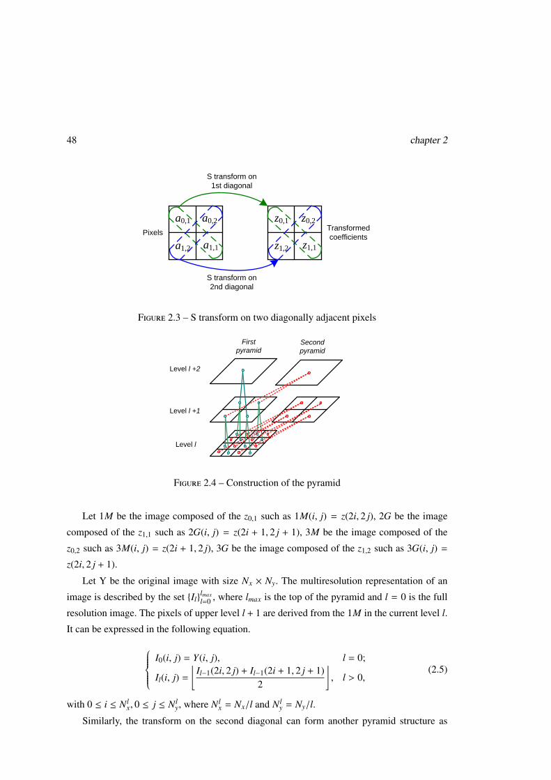
48 chapter 2
Source image Flat coder
LAR low
resolution image+
+
- TextureTexture coder
Source
image
Quadtree
Partitioning
Pyramid
building
Level 3
basic image
Level 2
basic image
Level 1
basic image
Level 0
basic image
Level 2
Texture
Level 1
Texture
Level 0
Texture
Entropy
coding
Quadtree partition data
a0,1
a1,1
a0,2
a1,2
z0,1
z1,1
z0,2
z1,2
Pixels Transformed
coefficients
S transform on
1st diagonal
S transform on
2nd diagonal
Figure 2.3 – S transform on two diagonally adjacent pixels
Source image Flat coder
LAR low
resolution image+
+
- TextureTexture coder
Source
image
Quadtree
Partitioning
Pyramid
building
Level 3
basic image
Level 2
basic image
Level 1
basic image
Level 0
basic image
Level 2
Texture
Level 1
Texture
Level 0
Texture
Entropy
coding
Quadtree partition data
a0,1
a1,1
a0,2
a1,2
z0,1
z1,1
z0,2
z1,2
Pixels Transformed
coefficients
S transform on
1st diagonal
S transform on
2nd diagonal Level l
Level l +1
Level l +2
First
pyramidSecond
pyramid
Figure 2.4 – Construction of the pyramid
Let 1M be the image composed of the z0,1 such as 1M(i, j) = z(2i, 2 j), 2G be the image
composed of the z1,1 such as 2G(i, j) = z(2i + 1, 2 j + 1), 3M be the image composed of the
z0,2 such as 3M(i, j) = z(2i + 1, 2 j), 3G be the image composed of the z1,2 such as 3G(i, j) =
z(2i, 2 j + 1).
Let Y be the original image with size Nx × Ny. The multiresolution representation of an
image is described by the set {Il}lmaxl=0 , where lmax is the top of the pyramid and l = 0 is the full
resolution image. The pixels of upper level l + 1 are derived from the 1M in the current level l.
It can be expressed in the following equation.
I0(i, j) = Y(i, j), l = 0;
Il(i, j) =
⌊Il−1(2i, 2 j) + Il−1(2i + 1, 2 j + 1)
2
⌋, l > 0,
(2.5)
with 0 ≤ i ≤ Nlx, 0 ≤ j ≤ Nl
y, where Nlx = Nx/l and Nl
y = Ny/l.
Similarly, the transform on the second diagonal can form another pyramid structure as
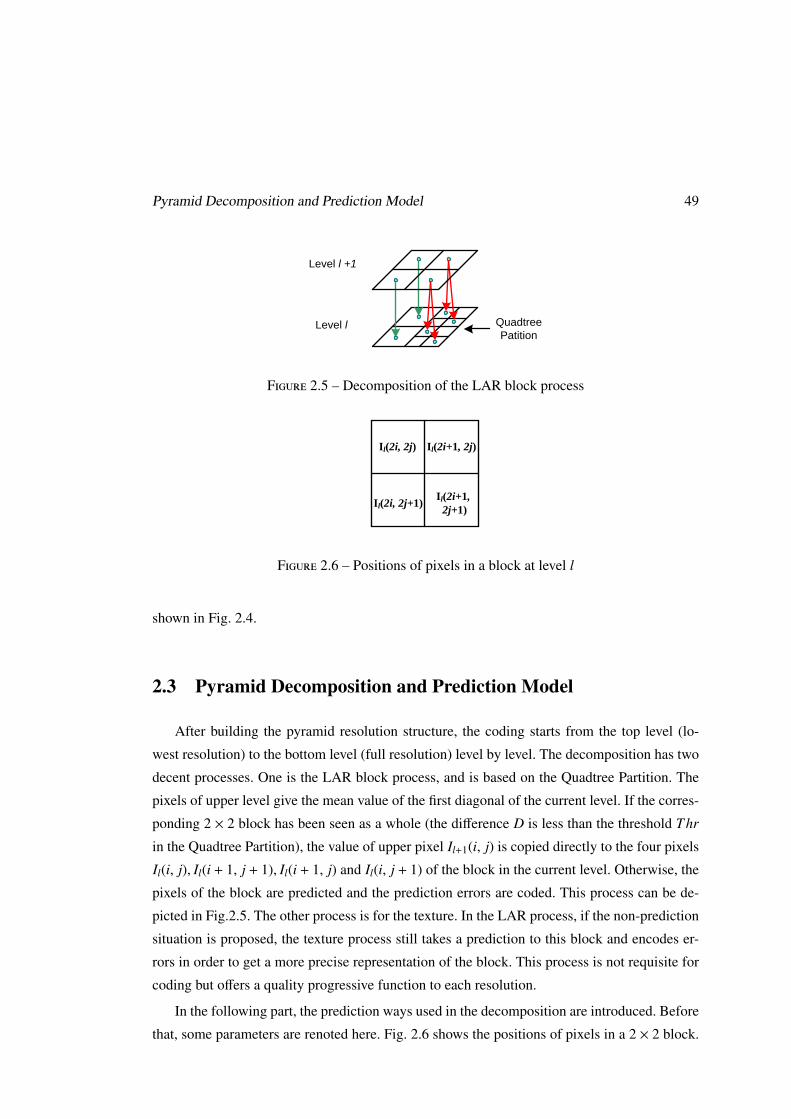
Pyramid Decomposition and Prediction Model 49
Source image Flat coder
LAR low
resolution image+
+
- TextureTexture coder
Source
image
Quadtree
Partitioning
Pyramid
building
Level 3
basic image
Level 2
basic image
Level 1
basic image
Level 0
basic image
Level 2
Texture
Level 1
Texture
Level 0
Texture
Entropy
coding
Quadtree partition data
a0,1
a1,1
a0,2
a1,2
z0,1
z1,1
z0,2
z1,2
Pixels Transformed
coefficients
S transform on
1st diagonal
S transform on
2nd diagonal Level l
Level l +1
Level l +2
First
pyramidSecond
pyramid
Level l
Level l +1
Quadtree
Patition
Figure 2.5 – Decomposition of the LAR block process
Source image Flat coder
LAR low
resolution image+
+
- TextureTexture coder
Source
image
Quadtree
Partitioning
Pyramid
building
Level 3
basic image
Level 2
basic image
Level 1
basic image
Level 0
basic image
Level 2
Texture
Level 1
Texture
Level 0
Texture
Entropy
coding
Quadtree partition data
a0,1
a1,1
a0,2
a1,2
z0,1
z1,1
z0,2
z1,2
Pixels Transformed
coefficients
S transform on
1st diagonal
S transform on
2nd diagonal Level l
Level l +1
Level l +2
First
pyramidSecond
pyramid
Level l
Level l +1
Quadtree
Patition
Il(2i, 2j)
Il(2i+1,
2j+1)
Il(2i+1, 2j)
Il(2i, 2j+1)
Figure 2.6 – Positions of pixels in a block at level l
shown in Fig. 2.4.
2.3 Pyramid Decomposition and Prediction Model
After building the pyramid resolution structure, the coding starts from the top level (lo-
west resolution) to the bottom level (full resolution) level by level. The decomposition has two
decent processes. One is the LAR block process, and is based on the Quadtree Partition. The
pixels of upper level give the mean value of the first diagonal of the current level. If the corres-
ponding 2 × 2 block has been seen as a whole (the difference D is less than the threshold Thr
in the Quadtree Partition), the value of upper pixel Il+1(i, j) is copied directly to the four pixels
Il(i, j), Il(i + 1, j + 1), Il(i + 1, j) and Il(i, j + 1) of the block in the current level. Otherwise, the
pixels of the block are predicted and the prediction errors are coded. This process can be de-
picted in Fig.2.5. The other process is for the texture. In the LAR process, if the non-prediction
situation is proposed, the texture process still takes a prediction to this block and encodes er-
rors in order to get a more precise representation of the block. This process is not requisite for
coding but offers a quality progressive function to each resolution.
In the following part, the prediction ways used in the decomposition are introduced. Before
that, some parameters are renoted here. Fig. 2.6 shows the positions of pixels in a 2 × 2 block.
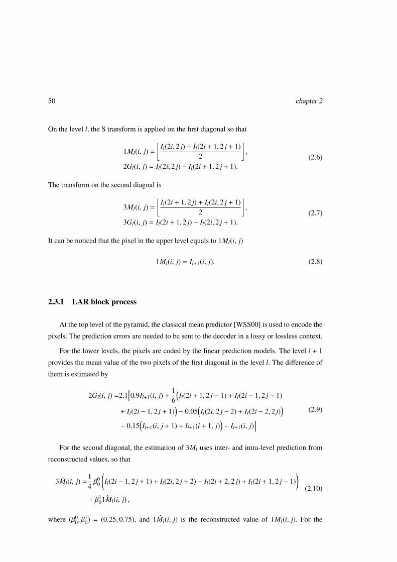
50 chapter 2
On the level l, the S transform is applied on the first diagonal so that
1Ml(i, j) =
⌊Il(2i, 2 j) + Il(2i + 1, 2 j + 1)
2
⌋,
2Gl(i, j) = Il(2i, 2 j) − Il(2i + 1, 2 j + 1).(2.6)
The transform on the second diagnal is
3Ml(i, j) =
⌊Il(2i + 1, 2 j) + Il(2i, 2 j + 1)
2
⌋,
3Gl(i, j) = Il(2i + 1, 2 j) − Il(2i, 2 j + 1).(2.7)
It can be noticed that the pixel in the upper level equals to 1Ml(i, j)
1Ml(i, j) = Il+1(i, j). (2.8)
2.3.1 LAR block process
At the top level of the pyramid, the classical mean predictor [WSS00] is used to encode the
pixels. The prediction errors are needed to be sent to the decoder in a lossy or lossless context.
For the lower levels, the pixels are coded by the linear prediction models. The level l + 1
provides the mean value of the two pixels of the first diagonal in the level l. The difference of
them is estimated by
2Gl(i, j) =2.1[0.9Il+1(i, j) +
16
(Il(2i + 1, 2 j − 1) + Il(2i − 1, 2 j − 1)
+ Il(2i − 1, 2 j + 1))− 0.05
(Il(2i, 2 j − 2) + Il(2i − 2, 2 j)
)− 0.15
(Il+1(i, j + 1) + Il+1(i + 1, j)
)− Il+1(i, j)
] (2.9)
For the second diagonal, the estimation of 3Ml uses inter- and intra-level prediction from
reconstructed values, so that
3Ml(i, j) =14β0
0
(Il(2i − 1, 2 j + 1) + Il(2i, 2 j + 2) − Il(2i + 2, 2 j) + Il(2i + 1, 2 j − 1)
)+ β1
0ˆ1Ml(i, j) ,
(2.10)
where (β00, β
10) = (0.25, 0.75), and 1Ml(i, j) is the reconstructed value of 1Ml(i, j). For the
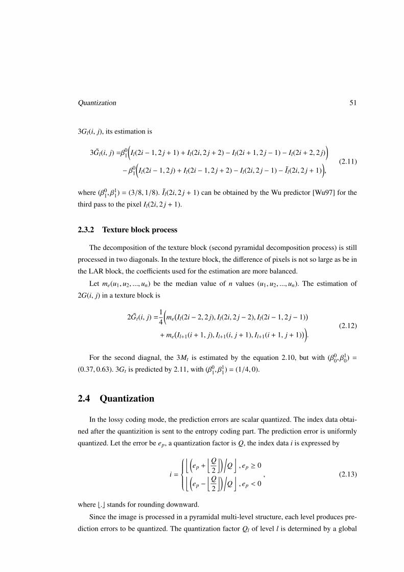
Quantization 51
3Gl(i, j), its estimation is
3Gl(i, j) =β01
(Il(2i − 1, 2 j + 1) + Il(2i, 2 j + 2) − Il(2i + 1, 2 j − 1) − Il(2i + 2, 2 j)
)− β0
1
(Il(2i − 1, 2 j) + Il(2i − 1, 2 j + 2) − Il(2i, 2 j − 1) − Il(2i, 2 j + 1)
),
(2.11)
where (β01, β
11) = (3/8, 1/8). Il(2i, 2 j + 1) can be obtained by the Wu predictor [Wu97] for the
third pass to the pixel Il(2i, 2 j + 1).
2.3.2 Texture block process
The decomposition of the texture block (second pyramidal decomposition process) is still
processed in two diagonals. In the texture block, the difference of pixels is not so large as be in
the LAR block, the coefficients used for the estimation are more balanced.
Let me(u1, u2, ..., un) be the median value of n values (u1, u2, ..., un). The estimation of
2G(i, j) in a texture block is
2Gt(i, j) =14
(me
(Il(2i − 2, 2 j), Il(2i, 2 j − 2), Il(2i − 1, 2 j − 1)
)+ me
(Il+1(i + 1, j), Il+1(i, j + 1), Il+1(i + 1, j + 1)
)).
(2.12)
For the second diagnal, the 3Mt is estimated by the equation 2.10, but with (β00, β
10) =
(0.37, 0.63). 3Gt is predicted by 2.11, with (β01, β
11) = (1/4, 0).
2.4 Quantization
In the lossy coding mode, the prediction errors are scalar quantized. The index data obtai-
ned after the quantizition is sent to the entropy coding part. The prediction error is uniformly
quantized. Let the error be ep, a quantization factor is Q, the index data i is expressed by
i =
⌊ (
ep +
⌊Q2
⌋) /Q
⌋, ep ≥ 0⌊ (
ep −
⌊Q2
⌋) /Q
⌋, ep < 0
, (2.13)
where b.c stands for rounding downward.
Since the image is processed in a pyramidal multi-level structure, each level produces pre-
diction errors to be quantized. The quantization factor Ql of level l is determined by a global
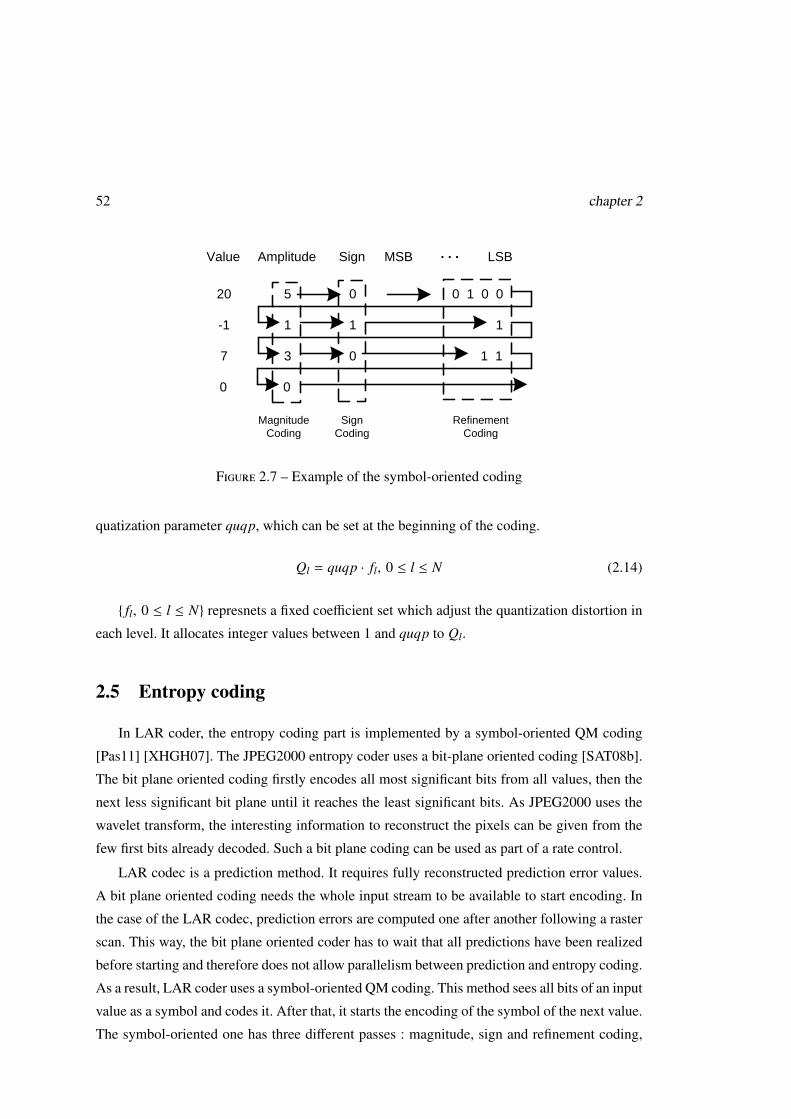
52 chapter 2
Source image Flat coder
LAR low
resolution image+
+
- TextureTexture coder
Source
image
Quadtree
Partitioning
Pyramid
building
Level 3
basic image
Level 2
basic image
Level 1
basic image
Level 0
basic image
Level 2
Texture
Level 1
Texture
Level 0
Texture
Entropy
coding
Quadtree partition data
a0,1
a1,1
a0,2
a1,2
z0,1
z1,1
z0,2
z1,2
Pixels Transformed
coefficients
S transform on
1st diagonal
S transform on
2nd diagonal Level l
Level l +1
Level l +2
First
pyramidSecond
pyramid
Level l
Level l +1
Quadtree
Patition
Il(2i, 2j)
Il(2i+1,
2j+1)
Il(2i+1, 2j)
Il(2i, 2j+1)
Value Amplitude Sign MSB LSB
20 5 0 0 1 0 0
. . .
-1 1 1
7 3 0
1
1 1
0 0
Magnitude
Coding
Sign
Coding
Refinement
Coding
Figure 2.7 – Example of the symbol-oriented coding
quatization parameter quqp, which can be set at the beginning of the coding.
Ql = quqp · fl, 0 ≤ l ≤ N (2.14)
{ fl, 0 ≤ l ≤ N} represnets a fixed coefficient set which adjust the quantization distortion in
each level. It allocates integer values between 1 and quqp to Ql.
2.5 Entropy coding
In LAR coder, the entropy coding part is implemented by a symbol-oriented QM coding
[Pas11] [XHGH07]. The JPEG2000 entropy coder uses a bit-plane oriented coding [SAT08b].
The bit plane oriented coding firstly encodes all most significant bits from all values, then the
next less significant bit plane until it reaches the least significant bits. As JPEG2000 uses the
wavelet transform, the interesting information to reconstruct the pixels can be given from the
few first bits already decoded. Such a bit plane coding can be used as part of a rate control.
LAR codec is a prediction method. It requires fully reconstructed prediction error values.
A bit plane oriented coding needs the whole input stream to be available to start encoding. In
the case of the LAR codec, prediction errors are computed one after another following a raster
scan. This way, the bit plane oriented coder has to wait that all predictions have been realized
before starting and therefore does not allow parallelism between prediction and entropy coding.
As a result, LAR coder uses a symbol-oriented QM coding. This method sees all bits of an input
value as a symbol and codes it. After that, it starts the encoding of the symbol of the next value.
The symbol-oriented one has three different passes : magnitude, sign and refinement coding,
Conclusion 53
as shown in Fig.2.7.
The magnitude coding has two functions in the coding. The first one is coding the number of
bits needed to represent the symbol to be encoded. The second one is to adjust the complexity of
the overall entropy coding by minimizing the number of coding passes needed. The magnitude
coding firstly computes the minimal number of bits A to represent the symbol A. Then, the bits
A are coded through unary coding with a dictionnary containing the length of the codeword.
Finally, each bit from the unary codeword is encoded with the QM Coder.
The sign is directly coded after the magnitude coding and the algorithm is not different from
the bit plane oriented QM Coding. At last, the remaining bits are encoded in the refinement
coding. The number of the refinement bits has been determined by the magnitude coding pass.
2.6 Conclusion
The LAR framework tends to associate the compression efficiency and the content-based
representation. It relies on an S transform based multiresolution representation. The coding
scheme involves the prediction, quantization and entropy coding of the quantized prediction
errors. The implementation of the LAR codec can complete both lossy and lossless coding
under the same coding structure.
Although the LAR codec has the complete and independent coding structure, it is not op-
timized for the rate-distortion. For the implementation, there are key parameters, such as the
Thr of the quadtree partition and the quqp of the quantization, play important roles for the
compression efficiency. The optimal collocations of parameters are not determined during the
coding. As a result, the coding efficiency is much limited. Since the original version of the LAR
codec aims at coding functionalities, the computation comlexity causes a more time consump-
tion than JPEG 2000. These problems make the LAR be not standardized successfully in the
JPEG-AIC response.
The main drawbacks of LAR codec are about its limited coding efficiency and the compu-
tation complexity. In my work, I firstly analyzed the main coding steps of LAR, next tried to
build models to describe the relation of key parameters and keeped the LAR codec work under
a configuration which is close to the optimal choice. Further, the subjective measurement is
taken into consideration and perceptual quality is improved at high bitrates.
Aiming at a low complexity efficient image codec, a new coding scheme is proposed and
achieved in lossless mode under the LAR framework. In this context, coding steps are changed
for better coding performance, and a classification module is introduced to decrease the entropy

54 chapter 2
of the prediction errors. The QM coding is also replaced by the classic Huffman coding for
less computation cost. This new coding scheme achieves a better lossless image compression
efficiency which is equivalent to the one of JPEG2000, while has much lower coding latency.
Chapter 3
Rate-distortion-optimization (RDO) mo-del for LAR codec
The rate-distortion-optimization (RDO) is an important issue for the image coding tech-
niques. Studies have been conducted on state of the art codecs to understand their behaviors
in terms of quality and/or rate. Such studies are often a step of a rate distortion optimization
design. For example, the impacts of quantization on the DCT coefficients for the JPEG codec
[YL96], and an improved algorithm for RDO in JPEG2000 [XGC+06].
Given a particular compression framework, there are often two ways to study the possible
optimization methods. One is to focus on the statistic properties of inside functions. It tries to
monitor each coding unit and adjust parameters during the coding so as to achieve a desirable
performance at a specific bitrate, such as the PCRD used in JPEG2000 1.2.3. This process
is effective but involves large of computation and possible required memory. Another way is
looking for the best operating points for that specific system. For example, consider a scalar
quantizer followed by an entropy coder. If all the quantization choices have been considered,
an operational rate-distortion curve can be defined and plotted by pairs of each bitrate and the
distortion achieved by designing the best codec for this bitrate. This curve can distinguish bet-
ween the best achievable operating points and those which are sub-optimal or unachievable. A
particular case is shown in Fig. 3.1. The encoder can select among a discrete set of coding pa-
rameters, such as a discrete set of quantization elements. The R-D points are obtained through
the choice of different combination of coding parameters. The individual admissible operating
points are connected to form a convex hull. This method tries to find the optimal rate-distortion
performance in the current compression framework. Once some key parameters are chosen, the
coding processes step by step without much adaptive modification. Thus it reduces the coding
55
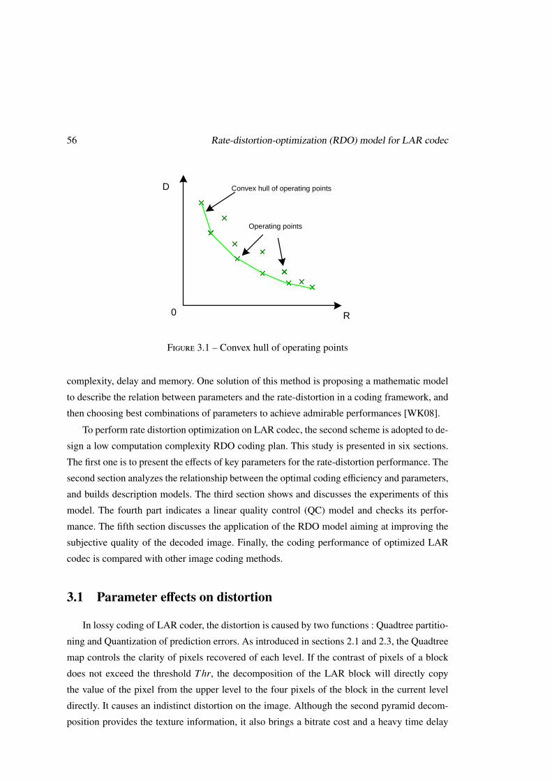
56 Rate-distortion-optimization (RDO) model for LAR codec
Convex hull of operating points
Operating points
R
D
0
Figure 3.1 – Convex hull of operating points
complexity, delay and memory. One solution of this method is proposing a mathematic model
to describe the relation between parameters and the rate-distortion in a coding framework, and
then choosing best combinations of parameters to achieve admirable performances [WK08].
To perform rate distortion optimization on LAR codec, the second scheme is adopted to de-
sign a low computation complexity RDO coding plan. This study is presented in six sections.
The first one is to present the effects of key parameters for the rate-distortion performance. The
second section analyzes the relationship between the optimal coding efficiency and parameters,
and builds description models. The third section shows and discusses the experiments of this
model. The fourth part indicates a linear quality control (QC) model and checks its perfor-
mance. The fifth section discusses the application of the RDO model aiming at improving the
subjective quality of the decoded image. Finally, the coding performance of optimized LAR
codec is compared with other image coding methods.
3.1 Parameter effects on distortion
In lossy coding of LAR coder, the distortion is caused by two functions : Quadtree partitio-
ning and Quantization of prediction errors. As introduced in sections 2.1 and 2.3, the Quadtree
map controls the clarity of pixels recovered of each level. If the contrast of pixels of a block
does not exceed the threshold Thr, the decomposition of the LAR block will directly copy
the value of the pixel from the upper level to the four pixels of the block in the current level
directly. It causes an indistinct distortion on the image. Although the second pyramid decom-
position provides the texture information, it also brings a bitrate cost and a heavy time delay
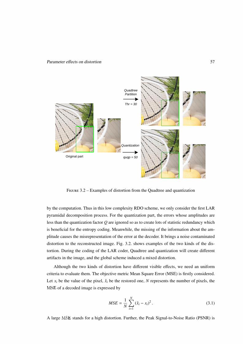
Parameter effects on distortion 57
Convex hull of operating points
Operating points
R
D
0
Original part
Thr = 30
Quadtree
Partition
quqp = 50
Quantization
Figure 3.2 – Examples of distortion from the Quadtree and quantization
by the computation. Thus in this low complexity RDO scheme, we only consider the first LAR
pyramidal decomposition process. For the quantization part, the errors whose amplitudes are
less than the quantization factor Q are ignored so as to create lots of statistic redundancy which
is beneficial for the entropy coding. Meanwhile, the missing of the information about the am-
plitude causes the misrepresentation of the error at the decoder. It brings a noise contaminated
distortion to the reconstructed image. Fig. 3.2. shows examples of the two kinds of the dis-
tortion. During the coding of the LAR coder, Quadtree and quantization will create different
artifacts in the image, and the global scheme induced a mixed distortion.
Although the two kinds of distortion have different visible effects, we need an uniform
criteria to evaluate them. The objective metric Mean Square Error (MSE) is firstly considered.
Let xi be the value of the pixel, xi be the restored one, N represents the number of pixels, the
MSE of a decoded image is expressed by
MSE =1N
N∑i=1
(xi − xi)2 . (3.1)
A large MSE stands for a high distortion. Further, the Peak Signal-to-Noise Ratio (PSNR) is
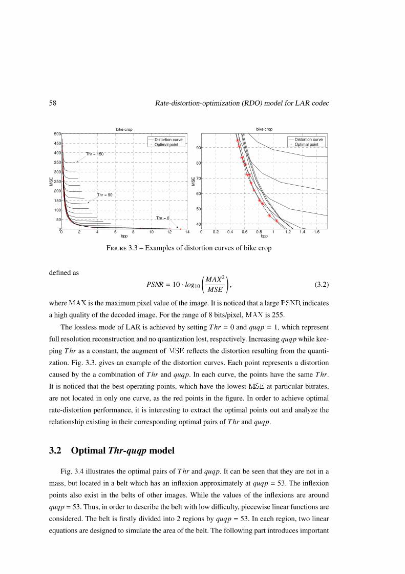
58 Rate-distortion-optimization (RDO) model for LAR codec
0 2 4 6 8 10 12 140
50
100
150
200
250
300
350
400
450
500
bpp
MS
E
bike crop
Distortion curve
Optimal point
Thr = 150
Thr = 90
Thr = 0
0 0.2 0.4 0.6 0.8 1 1.2 1.4 1.6
40
50
60
70
80
90
bpp
MS
E
bike crop
Distortion curve
Optimal point
Figure 3.3 – Examples of distortion curves of bike crop
defined as
PSNR = 10 · log10
(MAX2
MSE
), (3.2)
where MAX is the maximum pixel value of the image. It is noticed that a large PSNR indicates
a high quality of the decoded image. For the range of 8 bits/pixel, MAX is 255.
The lossless mode of LAR is achieved by setting Thr = 0 and quqp = 1, which represent
full resolution reconstruction and no quantization lost, respectively. Increasing quqp while kee-
ping Thr as a constant, the augment of MSE reflects the distortion resulting from the quanti-
zation. Fig. 3.3. gives an example of the distortion curves. Each point represents a distortion
caused by the a combination of Thr and quqp. In each curve, the points have the same Thr.
It is noticed that the best operating points, which have the lowest MSE at particular bitrates,
are not located in only one curve, as the red points in the figure. In order to achieve optimal
rate-distortion performance, it is interesting to extract the optimal points out and analyze the
relationship existing in their corresponding optimal pairs of Thr and quqp.
3.2 Optimal Thr-quqp model
Fig. 3.4 illustrates the optimal pairs of Thr and quqp. It can be seen that they are not in a
mass, but located in a belt which has an inflexion approximately at quqp = 53. The inflexion
points also exist in the belts of other images. While the values of the inflexions are around
quqp = 53. Thus, in order to describe the belt with low difficulty, piecewise linear functions are
considered. The belt is firstly divided into 2 regions by quqp = 53. In each region, two linear
equations are designed to simulate the area of the belt. The following part introduces important
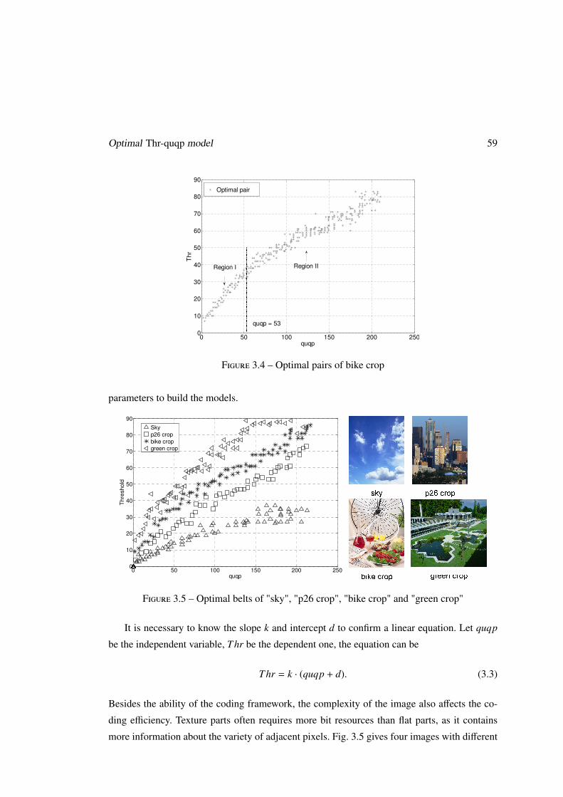
Optimal Thr-quqp model 59
0 2 4 6 8 10 12 140
50
100
150
200
250
300
350
400
450
500
bpp
MS
E
bike crop
Distortion curve
Optimal point
Thr = 150
Thr = 90
Thr = 0
0 0.2 0.4 0.6 0.8 1 1.2 1.4 1.6
40
50
60
70
80
90
bpp
MS
E
bike crop
Distortion curve
Optimal point
0 50 100 150 200 2500
10
20
30
40
50
60
70
80
90
quqp
Th
r
Optimal pair
quqp = 53
Region I Region II
Figure 3.4 – Optimal pairs of bike crop
parameters to build the models.
0 2 4 6 8 10 12 140
50
100
150
200
250
300
350
400
450
500
bpp
MS
E
bike crop
Distortion curve
Optimal point
Thr = 150
Thr = 90
Thr = 0
0 0.2 0.4 0.6 0.8 1 1.2 1.4 1.6
40
50
60
70
80
90
bpp
MS
E
bike crop
Distortion curve
Optimal point
0 50 100 150 200 2500
10
20
30
40
50
60
70
80
90
quqp
Thre
sho
ld
Sky
p26 crop
bike crop
green crop
0 50 100 150 200 2500
10
20
30
40
50
60
70
80
90
quqp
Th
r
Optimal pair
quqp = 53
Region I Region II
Figure 3.5 – Optimal belts of "sky", "p26 crop", "bike crop" and "green crop"
It is necessary to know the slope k and intercept d to confirm a linear equation. Let quqp
be the independent variable, Thr be the dependent one, the equation can be
Thr = k · (quqp + d). (3.3)
Besides the ability of the coding framework, the complexity of the image also affects the co-
ding efficiency. Texture parts often requires more bit resources than flat parts, as it contains
more information about the variety of adjacent pixels. Fig. 3.5 gives four images with different
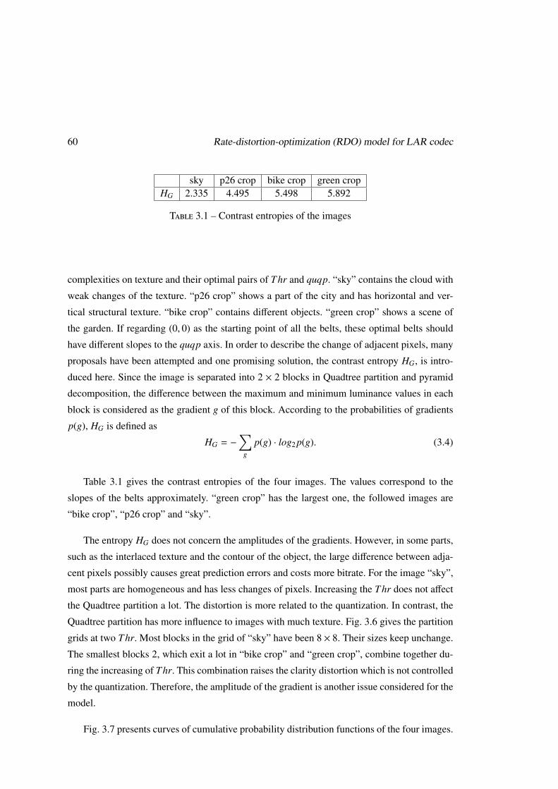
60 Rate-distortion-optimization (RDO) model for LAR codec
sky p26 crop bike crop green cropHG 2.335 4.495 5.498 5.892
Table 3.1 – Contrast entropies of the images
complexities on texture and their optimal pairs of Thr and quqp. “sky” contains the cloud with
weak changes of the texture. “p26 crop” shows a part of the city and has horizontal and ver-
tical structural texture. “bike crop” contains different objects. “green crop” shows a scene of
the garden. If regarding (0, 0) as the starting point of all the belts, these optimal belts should
have different slopes to the quqp axis. In order to describe the change of adjacent pixels, many
proposals have been attempted and one promising solution, the contrast entropy HG, is intro-
duced here. Since the image is separated into 2 × 2 blocks in Quadtree partition and pyramid
decomposition, the difference between the maximum and minimum luminance values in each
block is considered as the gradient g of this block. According to the probabilities of gradients
p(g), HG is defined as
HG = −∑
g
p(g) · log2 p(g). (3.4)
Table 3.1 gives the contrast entropies of the four images. The values correspond to the
slopes of the belts approximately. “green crop” has the largest one, the followed images are
“bike crop”, “p26 crop” and “sky”.
The entropy HG does not concern the amplitudes of the gradients. However, in some parts,
such as the interlaced texture and the contour of the object, the large difference between adja-
cent pixels possibly causes great prediction errors and costs more bitrate. For the image “sky”,
most parts are homogeneous and has less changes of pixels. Increasing the Thr does not affect
the Quadtree partition a lot. The distortion is more related to the quantization. In contrast, the
Quadtree partition has more influence to images with much texture. Fig. 3.6 gives the partition
grids at two Thr. Most blocks in the grid of “sky” have been 8 × 8. Their sizes keep unchange.
The smallest blocks 2, which exit a lot in “bike crop” and “green crop”, combine together du-
ring the increasing of Thr. This combination raises the clarity distortion which is not controlled
by the quantization. Therefore, the amplitude of the gradient is another issue considered for the
model.
Fig. 3.7 presents curves of cumulative probability distribution functions of the four images.
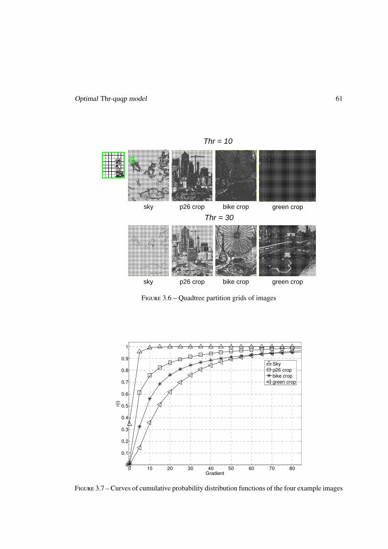
Optimal Thr-quqp model 61
sky
sky
p26 crop
p26 crop
bike crop
bike crop
green crop
green crop
Thr = 10
Thr = 30
0 10 20 30 40 50 60 70 80
0
0.1
0.2
0.3
0.4
0.5
0.6
0.7
0.8
0.9
1
Gradient
r(i)
Sky
p26 crop
bike crop
green crop
Figure 3.6 – Quadtree partition grids of images
0 10 20 30 40 50 60 70 800
0.1
0.2
0.3
0.4
0.5
0.6
0.7
0.8
0.9
1
Gradient
r(i)
Sky
p26 crop
bike crop
green crop
Figure 3.7 – Curves of cumulative probability distribution functions of the four example images
62 Rate-distortion-optimization (RDO) model for LAR codec
The gradient represents the values of the gradient g. The r(i) is defined as
r(i) =
i∑g=0
p(g). (3.5)
If an image has large portions of the same color and moderate transitions, most gradients have
small values and the r(i) curve rises more quickly as the “sky” one. The cumulation curve
becomes close to 1 even the gradient is only 10. after that, since r(i) is no more than 1, the
increasing of the curve becomes very small. For the “green” one, the curve rises much slower
and r(i) reaches 0.9 at Gradient = 50. The rate of rise is obvious and comparable before reaching
the flat part where r(i) is close to 1. There are two choices to reflect the rising speed. One is
to fix a threshold, such as r(i) = 0.9. Each image has its own value of i when its r(i) curve
reaches 0.9. The images with much texture information have a wide range of the gradient. The
curve increases slowly and get a large i, as the one of “green crop” in Fig. 3.7. However, the
threshold are not constant exactly. The r(i − 1) may be lower than 0.9 but r(i) rises to 0.92
or more, especially for the simply structured image with the sharp rising of r(i). It is not fair
for the comparison. The other solution used here is choosing a range of the gradient [id, iu ]
and calculate the difference of r(i). A large difference indicates that lots of gradients fall in
this range. In Fig. 3.7, the curves become more steady after i = 45. Before that, the curves
rise in different speeds and locate separately. The difference between r(0) and r(45) would be
a choice to represent their speeds. However, r(0) is quite small for the textured images. The
difference between r(0) and r(45) mainly depends on the values of r(45) which do not differ
much between images. In order to distinguish the difference between [id, iu ] obviously, the
lower bound id is increased to 7 and the difference between r(45) and r(7) is used to evaluate
the slope of a r-curve. From the Fig.3.7, the “green crop” has the largest difference while the
“sky” one is the least.
∆ = r(45) − r(7) (3.6)
According to the study above, the RDO linear model is firstly formed as
Thr =HG
α(quqp + ∆ · β). (3.7)
HG contributes to the slope. For images with less textures, ∆ has a small value in order to
slow the augment of Thr. α and β are coefficients trying to map the models according with
the distribution of the optimal belt. These coefficients are constant and achieved by the curve
fitting.
Optimal Thr-quqp model 63
The objective of curve fitting is to theoretically describe experimental data with a model
(function or equation) and to find the parameters associated with this model. In this section,
the curve fitting is applied to find the values of the coefficients, α and β, which make the RDO
model match the data of the optimal quqp-Thr belt as closely as possible. The best values of
the coefficients are the ones that minimize the value of the summed square of residuals, which
is given by
SR =
n∑i=1
(yi − yi)2 (3.8)
where y is a fitted value for a given point, yi is the measured data value for the point, n is the
number of data points included in the fit and SR is the sum of square of residuals. 8 cropped
images from the ISO 12640 JPEG test set and 12 free images in high resolution are taken out to
form a training set. The RDO model is trained for each image to get a pair of corresponding α
and β by the curve fitting. Indeed, the values of (α, β) of images are different but wave in a small
range. Therefore, the average value of α and the average one of β, α = 17.93 and β = 121.07,
are chosen as the coefficients of the model. Noticing the equation (3.7) does not go through
the original point, it is used for the region II. However, this equation can provide the crossover
point C (quqp = 53,Thr = Thrquqp=53), which should exit in both linear models of the region
I and II. Considering the two points (0, 0) and C, the linear model for the region I can also be
obtained
Thr =HG
α(1 +
∆ · β
53) quqp. (3.9)
Since the belt has the width, a distance, 10, in the Thr direction is used to shift the linear model
so as to cover the possible area of the belt. The proposed RDO model is expressed as
Thr2,1 =
HG
α(quqp + ∆ · β)
Thr2,2 =HG
α(quqp + ∆ · β) + 10
, i f quqp ≥ 53
Thr1,1 =
HG
α(1 +
∆ · β
53) quqp
Thr1,2 =HG
α(1 +
∆ · β
53) quqp + 10
, i f 0 < quqp < 53
(3.10)
where Thri,1 is the model 1 for the region i (i = 1, 2) and Thri,2 is the model 2. The two models
try to simulate the boundaries of the belt. During the practical coding, the average value of
model 1 and 2 is chosen as Thr.
Thr = (Thri,1 + Thri,2)/2 (3.11)
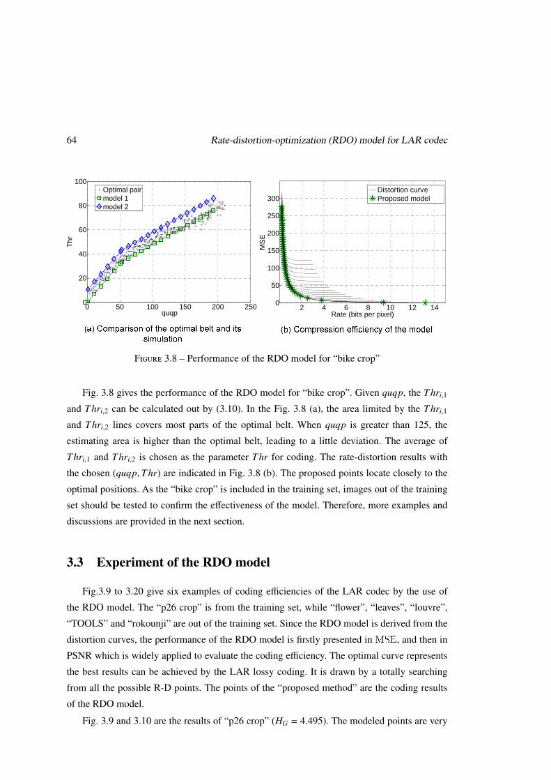
64 Rate-distortion-optimization (RDO) model for LAR codec
0 50 100 150 200 2500
20
40
60
80
100
quqp
Thr
Optimal pairmodel 1model 2
2 4 6 8 10 12 140
50
100
150
200
250
300
Rate (bits per pixel)
MS
E
Distortion curveProposed model
Figure 3.8 – Performance of the RDO model for “bike crop”
Fig. 3.8 gives the performance of the RDO model for “bike crop”. Given quqp, the Thri,1
and Thri,2 can be calculated out by (3.10). In the Fig. 3.8 (a), the area limited by the Thri,1
and Thri,2 lines covers most parts of the optimal belt. When quqp is greater than 125, the
estimating area is higher than the optimal belt, leading to a little deviation. The average of
Thri,1 and Thri,2 is chosen as the parameter Thr for coding. The rate-distortion results with
the chosen (quqp,Thr) are indicated in Fig. 3.8 (b). The proposed points locate closely to the
optimal positions. As the “bike crop” is included in the training set, images out of the training
set should be tested to confirm the effectiveness of the model. Therefore, more examples and
discussions are provided in the next section.
3.3 Experiment of the RDO model
Fig.3.9 to 3.20 give six examples of coding efficiencies of the LAR codec by the use of
the RDO model. The “p26 crop” is from the training set, while “flower”, “leaves”, “louvre”,
“TOOLS” and “rokounji” are out of the training set. Since the RDO model is derived from the
distortion curves, the performance of the RDO model is firstly presented in MSE, and then in
PSNR which is widely applied to evaluate the coding efficiency. The optimal curve represents
the best results can be achieved by the LAR lossy coding. It is drawn by a totally searching
from all the possible R-D points. The points of the “proposed method” are the coding results
of the RDO model.
Fig. 3.9 and 3.10 are the results of “p26 crop” (HG = 4.495). The modeled points are very
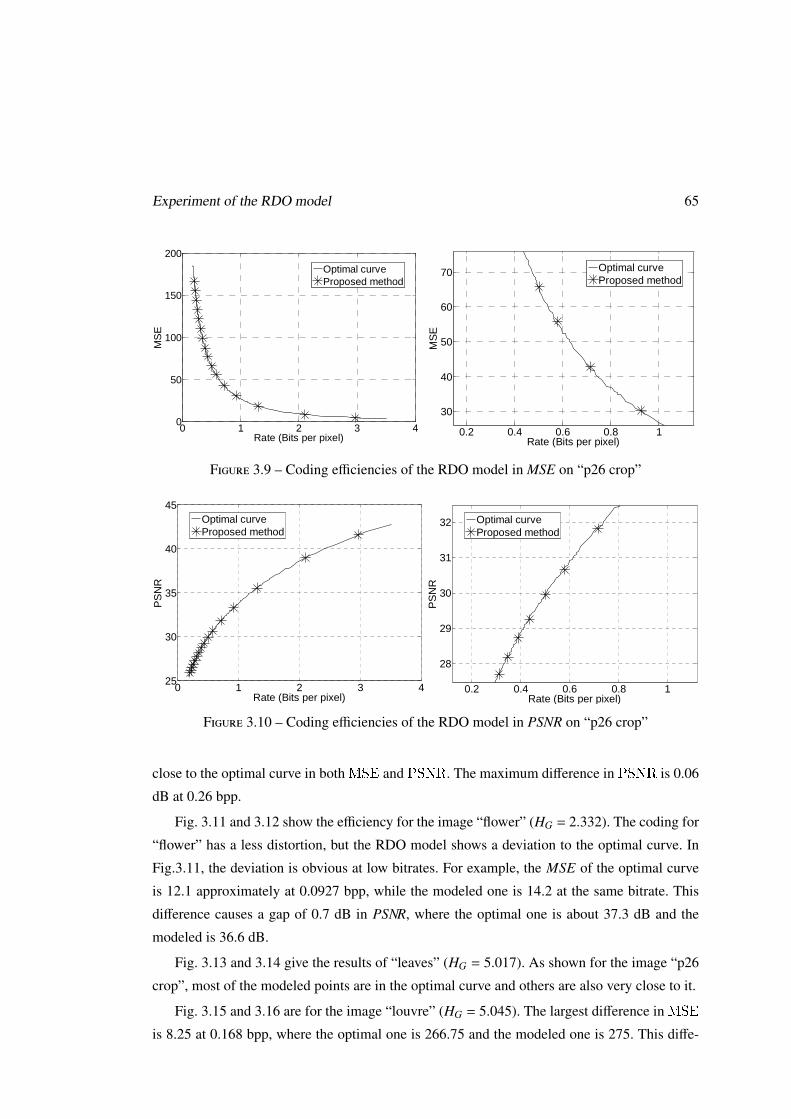
Experiment of the RDO model 65
0 1 2 3 40
50
100
150
200
Rate (Bits per pixel)
MS
E
Optimal curveProposed method
0.2 0.4 0.6 0.8 1
30
40
50
60
70
Rate (Bits per pixel)M
SE
Optimal curveProposed method
0 0.5 1 1.5 2 2.5 30
5
10
15
20
25
30
35
Rate (bits per pixel)
MS
E
Optimal curveProposed method
0 0.2 0.4 0.63
4
5
6
7
8
9
10
11
Rate (bits per pixel)
MS
E
Optimal curveProposed method
0 2 4 6 80
20
40
60
80
100
120
Rate (bits per pixel)
MS
E
Optimal curveProposed method
0.5 1 1.5 210
15
20
25
30
35
Rate (bits per pixel)
MS
E
Optimal curveProposed method
0 1 2 3 4 50
50
100
150
200
250
300
Rate (bits per pixel)
MS
E
Optimal curveProposed method
0.2 0.4 0.6 0.8 1 1.2 1.420
30
40
50
60
70
80
90
Rate (bits per pixel)
MS
E
Optimal curveProposed method
1.5 2 2.5 3 3.5
60
80
100
120
140
160
Rate (Bits per pixel)
MS
E
Optimal curveProposed method
0 2 4 6 8 100
50
100
150
200
250
300
350
400
450
Rate (Bits per pixel)
MS
E
Optimal curveProposed method
0 1 2 3 4 5 60
10
20
30
40
50
Rate (Bites per pixel)
MS
E
Optimal curveProposed Method
0 0.5 1 1.5 2 2.5
10
15
20
25
30
Rate (Bites per pixel)
MS
E
Optimal curveProposed Method
Figure 3.9 – Coding efficiencies of the RDO model in MSE on “p26 crop”
0 1 2 3 425
30
35
40
45
Rate (Bits per pixel)
PS
NR
Optimal curveProposed method
0.2 0.4 0.6 0.8 1
28
29
30
31
32
Rate (Bits per pixel)
PS
NR
Optimal curveProposed method
0 0.1 0.2 0.3 0.4 0.5 0.636.5
37
37.5
38
38.5
39
39.5
40
40.5
Rate (Bits per pixel)
PS
NR
Optimal curveProposed method
0 0.5 1 1.5 2 2.5 332
34
36
38
40
42
44
46
48
50
Rate (Bits per pixel)
PS
NR
Optimal curveProposed method
0 1 2 3 4 5 6 725
30
35
40
45
50
Rate (Bits per pixel)
PS
NR
Optimal curveProposed method
0.5 1 1.5 2
31
32
33
34
35
36
Rate (Bits per pixel)
PS
NR
Optimal curveProposed method
Figure 3.10 – Coding efficiencies of the RDO model in PSNR on “p26 crop”
close to the optimal curve in both MSE and PSNR. The maximum difference in PSNR is 0.06
dB at 0.26 bpp.
Fig. 3.11 and 3.12 show the efficiency for the image “flower” (HG = 2.332). The coding for
“flower” has a less distortion, but the RDO model shows a deviation to the optimal curve. In
Fig.3.11, the deviation is obvious at low bitrates. For example, the MSE of the optimal curve
is 12.1 approximately at 0.0927 bpp, while the modeled one is 14.2 at the same bitrate. This
difference causes a gap of 0.7 dB in PSNR, where the optimal one is about 37.3 dB and the
modeled is 36.6 dB.
Fig. 3.13 and 3.14 give the results of “leaves” (HG = 5.017). As shown for the image “p26
crop”, most of the modeled points are in the optimal curve and others are also very close to it.
Fig. 3.15 and 3.16 are for the image “louvre” (HG = 5.045). The largest difference in MSE
is 8.25 at 0.168 bpp, where the optimal one is 266.75 and the modeled one is 275. This diffe-
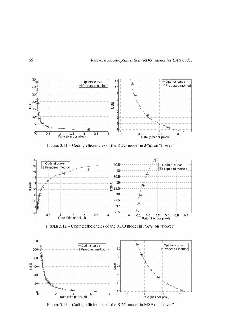
66 Rate-distortion-optimization (RDO) model for LAR codec0 1 2 3 4
0
50
100
150
200
Rate (Bits per pixel)
MS
E
Optimal curveProposed method
0.2 0.4 0.6 0.8 1
30
40
50
60
70
Rate (Bits per pixel)
MS
E
Optimal curveProposed method
0 0.5 1 1.5 2 2.5 30
5
10
15
20
25
30
35
Rate (bits per pixel)
MS
E
Optimal curveProposed method
0 0.2 0.4 0.63
4
5
6
7
8
9
10
11
Rate (bits per pixel)
MS
E
Optimal curveProposed method
0 2 4 6 80
20
40
60
80
100
120
Rate (bits per pixel)
MS
E
Optimal curveProposed method
0.5 1 1.5 210
15
20
25
30
35
Rate (bits per pixel)
MS
E
Optimal curveProposed method
0 1 2 3 4 50
50
100
150
200
250
300
Rate (bits per pixel)
MS
E
Optimal curveProposed method
0.2 0.4 0.6 0.8 1 1.2 1.420
30
40
50
60
70
80
90
Rate (bits per pixel)
MS
E
Optimal curveProposed method
1.5 2 2.5 3 3.5
60
80
100
120
140
160
Rate (Bits per pixel)
MS
E
Optimal curveProposed method
0 2 4 6 8 100
50
100
150
200
250
300
350
400
450
Rate (Bits per pixel)
MS
E
Optimal curveProposed method
0 1 2 3 4 5 60
10
20
30
40
50
Rate (Bites per pixel)
MS
E
Optimal curveProposed Method
0 0.5 1 1.5 2 2.5
10
15
20
25
30
Rate (Bites per pixel)
MS
E
Optimal curveProposed Method
Figure 3.11 – Coding efficiencies of the RDO model in MSE on “flower”
0 1 2 3 425
30
35
40
45
Rate (Bits per pixel)
PS
NR
Optimal curveProposed method
0.2 0.4 0.6 0.8 1
28
29
30
31
32
Rate (Bits per pixel)
PS
NR
Optimal curveProposed method
0 0.1 0.2 0.3 0.4 0.5 0.636.5
37
37.5
38
38.5
39
39.5
40
40.5
Rate (Bits per pixel)
PS
NR
Optimal curveProposed method
0 0.5 1 1.5 2 2.5 332
34
36
38
40
42
44
46
48
50
Rate (Bits per pixel)
PS
NR
Optimal curveProposed method
0 1 2 3 4 5 6 725
30
35
40
45
50
Rate (Bits per pixel)
PS
NR
Optimal curveProposed method
0.5 1 1.5 2
31
32
33
34
35
36
Rate (Bits per pixel)
PS
NR
Optimal curveProposed method
Figure 3.12 – Coding efficiencies of the RDO model in PSNR on “flower”
0 1 2 3 40
50
100
150
200
Rate (Bits per pixel)
MS
E
Optimal curveProposed method
0.2 0.4 0.6 0.8 1
30
40
50
60
70
Rate (Bits per pixel)
MS
E
Optimal curveProposed method
0 0.5 1 1.5 2 2.5 30
5
10
15
20
25
30
35
Rate (bits per pixel)
MS
E
Optimal curveProposed method
0 0.2 0.4 0.63
4
5
6
7
8
9
10
11
Rate (bits per pixel)
MS
E
Optimal curveProposed method
0 2 4 6 80
20
40
60
80
100
120
Rate (bits per pixel)
MS
E
Optimal curveProposed method
0.5 1 1.5 210
15
20
25
30
35
Rate (bits per pixel)
MS
E
Optimal curveProposed method
0 1 2 3 4 50
50
100
150
200
250
300
Rate (bits per pixel)
MS
E
Optimal curveProposed method
0.2 0.4 0.6 0.8 1 1.2 1.420
30
40
50
60
70
80
90
Rate (bits per pixel)
MS
E
Optimal curveProposed method
1.5 2 2.5 3 3.5
60
80
100
120
140
160
Rate (Bits per pixel)
MS
E
Optimal curveProposed method
0 2 4 6 8 100
50
100
150
200
250
300
350
400
450
Rate (Bits per pixel)
MS
E
Optimal curveProposed method
0 1 2 3 4 5 60
10
20
30
40
50
Rate (Bites per pixel)
MS
E
Optimal curveProposed Method
0 0.5 1 1.5 2 2.5
10
15
20
25
30
Rate (Bites per pixel)
MS
E
Optimal curveProposed Method
Figure 3.13 – Coding efficiencies of the RDO model in MSE on “leaves”
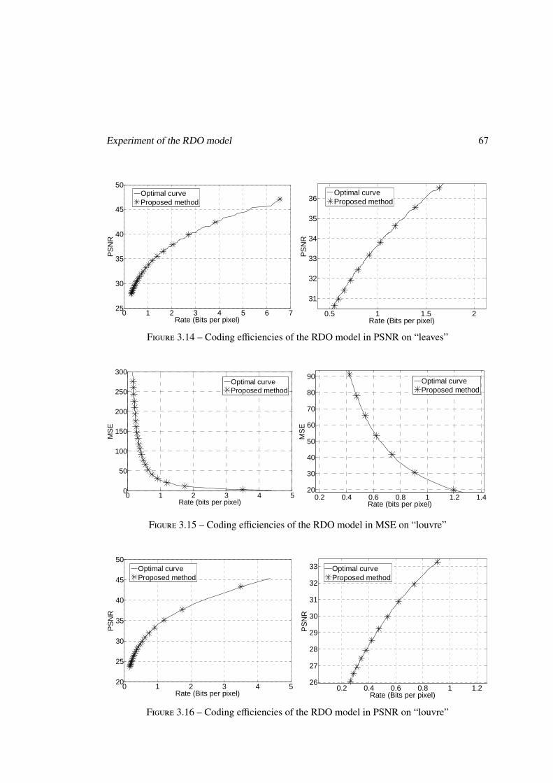
Experiment of the RDO model 67
0 1 2 3 425
30
35
40
45
Rate (Bits per pixel)
PS
NR
Optimal curveProposed method
0.2 0.4 0.6 0.8 1
28
29
30
31
32
Rate (Bits per pixel)
PS
NR
Optimal curveProposed method
0 0.1 0.2 0.3 0.4 0.5 0.636.5
37
37.5
38
38.5
39
39.5
40
40.5
Rate (Bits per pixel)
PS
NR
Optimal curveProposed method
0 0.5 1 1.5 2 2.5 332
34
36
38
40
42
44
46
48
50
Rate (Bits per pixel)
PS
NR
Optimal curveProposed method
0 1 2 3 4 5 6 725
30
35
40
45
50
Rate (Bits per pixel)
PS
NR
Optimal curveProposed method
0.5 1 1.5 2
31
32
33
34
35
36
Rate (Bits per pixel)
PS
NR
Optimal curveProposed method
Figure 3.14 – Coding efficiencies of the RDO model in PSNR on “leaves”
0 1 2 3 40
50
100
150
200
Rate (Bits per pixel)
MS
E
Optimal curveProposed method
0.2 0.4 0.6 0.8 1
30
40
50
60
70
Rate (Bits per pixel)
MS
E
Optimal curveProposed method
0 0.5 1 1.5 2 2.5 30
5
10
15
20
25
30
35
Rate (bits per pixel)
MS
E
Optimal curveProposed method
0 0.2 0.4 0.63
4
5
6
7
8
9
10
11
Rate (bits per pixel)
MS
E
Optimal curveProposed method
0 2 4 6 80
20
40
60
80
100
120
Rate (bits per pixel)
MS
E
Optimal curveProposed method
0.5 1 1.5 210
15
20
25
30
35
Rate (bits per pixel)
MS
E
Optimal curveProposed method
0 1 2 3 4 50
50
100
150
200
250
300
Rate (bits per pixel)
MS
E
Optimal curveProposed method
0.2 0.4 0.6 0.8 1 1.2 1.420
30
40
50
60
70
80
90
Rate (bits per pixel)
MS
E
Optimal curveProposed method
1.5 2 2.5 3 3.5
60
80
100
120
140
160
Rate (Bits per pixel)
MS
E
Optimal curveProposed method
0 2 4 6 8 100
50
100
150
200
250
300
350
400
450
Rate (Bits per pixel)
MS
E
Optimal curveProposed method
0 1 2 3 4 5 60
10
20
30
40
50
Rate (Bites per pixel)
MS
E
Optimal curveProposed Method
0 0.5 1 1.5 2 2.5
10
15
20
25
30
Rate (Bites per pixel)
MS
E
Optimal curveProposed Method
Figure 3.15 – Coding efficiencies of the RDO model in MSE on “louvre”
0 1 2 3 4 520
25
30
35
40
45
50
Rate (Bits per pixel)
PS
NR
Optimal curveProposed method
0.2 0.4 0.6 0.8 1 1.226
27
28
29
30
31
32
33
Rate (Bits per pixel)
PS
NR
Optimal curveProposed method
0 2 4 6 8 1020
25
30
35
40
45
Rate (Bits per pixel)
PS
NR
Optimal curveProposed method
0.5 1 1.5 2 2.522
23
24
25
26
27
28
Rate (Bits per pixel)
PS
NR
Optimal curveProposed method
0 1 2 3 4 5 630
32
34
36
38
40
42
44
46
Rate (Bits per pixel)
PS
NR
Optimal curveProposed method
0.2 0.4 0.6 0.8 1 1.2 1.433
33.5
34
34.5
35
35.5
36
36.5
Rate (Bits per pixel)
PS
NR
Optimal curveProposed method
Figure 3.16 – Coding efficiencies of the RDO model in PSNR on “louvre”
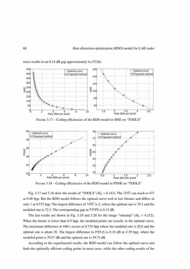
68 Rate-distortion-optimization (RDO) model for LAR codec
rence results in an 0.14 dB gap approximately in PSNR.
0 1 2 3 40
50
100
150
200
Rate (Bits per pixel)
MS
E
Optimal curveProposed method
0.2 0.4 0.6 0.8 1
30
40
50
60
70
Rate (Bits per pixel)
MS
E
Optimal curveProposed method
0 0.5 1 1.5 2 2.5 30
5
10
15
20
25
30
35
Rate (bits per pixel)
MS
E
Optimal curveProposed method
0 0.2 0.4 0.63
4
5
6
7
8
9
10
11
Rate (bits per pixel)
MS
E
Optimal curveProposed method
0 2 4 6 80
20
40
60
80
100
120
Rate (bits per pixel)
MS
E
Optimal curveProposed method
0.5 1 1.5 210
15
20
25
30
35
Rate (bits per pixel)
MS
E
Optimal curveProposed method
0 1 2 3 4 50
50
100
150
200
250
300
Rate (bits per pixel)
MS
E
Optimal curveProposed method
0.2 0.4 0.6 0.8 1 1.2 1.420
30
40
50
60
70
80
90
Rate (bits per pixel)
MS
E
Optimal curveProposed method
1.5 2 2.5 3 3.5
60
80
100
120
140
160
Rate (Bits per pixel)
MS
E
Optimal curveProposed method
0 2 4 6 8 100
50
100
150
200
250
300
350
400
450
Rate (Bits per pixel)
MS
E
Optimal curveProposed method
0 1 2 3 4 5 60
10
20
30
40
50
Rate (Bites per pixel)
MS
E
Optimal curveProposed Method
0 0.5 1 1.5 2 2.5
10
15
20
25
30
Rate (Bites per pixel)
MS
E
Optimal curveProposed Method
Figure 3.17 – Coding efficiencies of the RDO model in MSE on “TOOLS”
0 1 2 3 4 520
25
30
35
40
45
50
Rate (Bits per pixel)
PS
NR
Optimal curveProposed method
0.2 0.4 0.6 0.8 1 1.226
27
28
29
30
31
32
33
Rate (Bits per pixel)
PS
NR
Optimal curveProposed method
0 2 4 6 8 1020
25
30
35
40
45
Rate (Bits per pixel)
PS
NR
Optimal curveProposed method
0.5 1 1.5 2 2.522
23
24
25
26
27
28
Rate (Bits per pixel)
PS
NR
Optimal curveProposed method
0 1 2 3 4 5 630
32
34
36
38
40
42
44
46
Rate (Bits per pixel)
PS
NR
Optimal curveProposed method
0.2 0.4 0.6 0.8 1 1.2 1.433
33.5
34
34.5
35
35.5
36
36.5
Rate (Bits per pixel)
PS
NR
Optimal curveProposed method
Figure 3.18 – Coding efficiencies of the RDO model in PSNR on “TOOLS”
Fig. 3.17 and 3.18 show the results of “TOOLS” (HG = 6.143). The MSE can reach to 437
at 0.48 bpp. But the RDO model follows the optimal curve well at low bitrates and differs in
only 1 at 0.572 bpp. The largest difference of MSE is 2, where the optimal one is 70.3 and the
modeled one is 72.3. The corresponding gap in PSNR is 0.12 dB.
The last results are shown in Fig. 3.19 and 3.20 for the image “rokounji” (HG = 4.152).
When the bitrate is lower than 0.5 bpp, the modeled points are exactly in the optimal curve.
The maximum difference in MSE occurs at 0.735 bpp where the modeled one is 20.8 and the
optimal one is about 20. The largest difference in PSNR is 0.18 dB at 2.39 bpp, where the
modeled point is 39.57 dB and the optimal one is 39.75 dB.
According to the experimental results, the RDO model can follow the optimal curve and
finds the optimally efficient coding points in most cases, while the other coding results of the
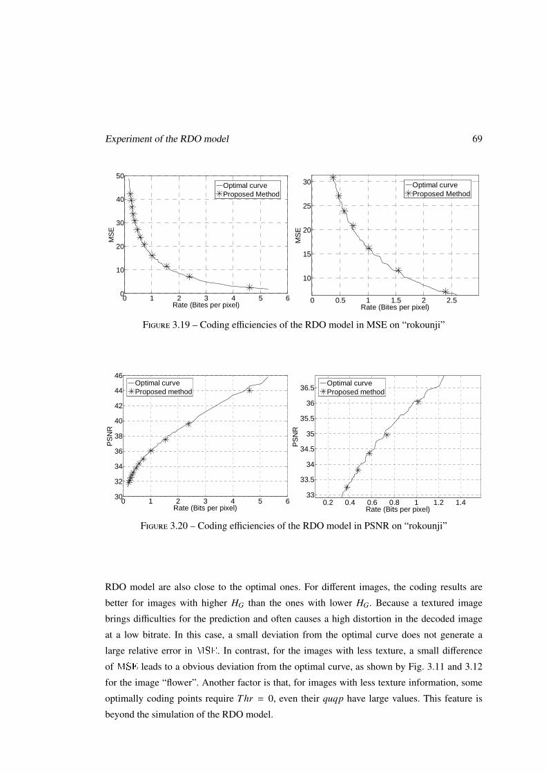
Experiment of the RDO model 69
0 1 2 3 40
50
100
150
200
Rate (Bits per pixel)
MS
E
Optimal curveProposed method
0.2 0.4 0.6 0.8 1
30
40
50
60
70
Rate (Bits per pixel)
MS
E
Optimal curveProposed method
0 0.5 1 1.5 2 2.5 30
5
10
15
20
25
30
35
Rate (bits per pixel)
MS
E
Optimal curveProposed method
0 0.2 0.4 0.63
4
5
6
7
8
9
10
11
Rate (bits per pixel)
MS
E
Optimal curveProposed method
0 2 4 6 80
20
40
60
80
100
120
Rate (bits per pixel)
MS
E
Optimal curveProposed method
0.5 1 1.5 210
15
20
25
30
35
Rate (bits per pixel)
MS
E
Optimal curveProposed method
0 1 2 3 4 50
50
100
150
200
250
300
Rate (bits per pixel)
MS
E
Optimal curveProposed method
0.2 0.4 0.6 0.8 1 1.2 1.420
30
40
50
60
70
80
90
Rate (bits per pixel)
MS
E
Optimal curveProposed method
1.5 2 2.5 3 3.5
60
80
100
120
140
160
Rate (Bits per pixel)
MS
E
Optimal curveProposed method
0 2 4 6 8 100
50
100
150
200
250
300
350
400
450
Rate (Bits per pixel)
MS
E
Optimal curveProposed method
0 1 2 3 4 5 60
10
20
30
40
50
Rate (Bites per pixel)
MS
E
Optimal curveProposed Method
0 0.5 1 1.5 2 2.5
10
15
20
25
30
Rate (Bites per pixel)M
SE
Optimal curveProposed Method
Figure 3.19 – Coding efficiencies of the RDO model in MSE on “rokounji”
0 1 2 3 4 520
25
30
35
40
45
50
Rate (Bits per pixel)
PS
NR
Optimal curveProposed method
0.2 0.4 0.6 0.8 1 1.226
27
28
29
30
31
32
33
Rate (Bits per pixel)
PS
NR
Optimal curveProposed method
0 2 4 6 8 1020
25
30
35
40
45
Rate (Bits per pixel)
PS
NR
Optimal curveProposed method
0.5 1 1.5 2 2.522
23
24
25
26
27
28
Rate (Bits per pixel)
PS
NR
Optimal curveProposed method
0 1 2 3 4 5 630
32
34
36
38
40
42
44
46
Rate (Bits per pixel)
PS
NR
Optimal curveProposed method
0.2 0.4 0.6 0.8 1 1.2 1.433
33.5
34
34.5
35
35.5
36
36.5
Rate (Bits per pixel)
PS
NR
Optimal curveProposed method
Figure 3.20 – Coding efficiencies of the RDO model in PSNR on “rokounji”
RDO model are also close to the optimal ones. For different images, the coding results are
better for images with higher HG than the ones with lower HG. Because a textured image
brings difficulties for the prediction and often causes a high distortion in the decoded image
at a low bitrate. In this case, a small deviation from the optimal curve does not generate a
large relative error in MSE. In contrast, for the images with less texture, a small difference
of MSE leads to a obvious deviation from the optimal curve, as shown by Fig. 3.11 and 3.12
for the image “flower”. Another factor is that, for images with less texture information, some
optimally coding points require Thr = 0, even their quqp have large values. This feature is
beyond the simulation of the RDO model.
70 Rate-distortion-optimization (RDO) model for LAR codec
3.4 Quality Control
Rate-distortion optimization (RDO) schemes aim at optimizing compression performance.
Depending on the RDO, functionalities, such as Rate Control (RC) and Quality Control (QC),
can realize practical applications during the coding. RC enables to compress the images at
a given rate. Its techniques are coding technique dependent, with various original possibility
of the coder. For example, besides the PCRD 1.2.3, JPEG2000 provides an embedded stream
enabling a fine RC [CLC08], [ZWD11]. Recently, RDO-domain has been introduced as an
efficient RC technique for H.264 [LLW10].
Besides, QC is also an important function. For the data storage and quality preferred ap-
plications, such as the archive recording, medical imaging and High Definition Television
(HDTV), the quality of the decoded image is the most concerning issue to the users. Recent
works of QC mostly focus on the perceptual quality metric. In [LKW06], a vision model was
proposed to incorporate various masking effects of human visual perception and a perceptual
distortion metric. This model was applied into JPEG2000 to control the embedded bit-plane
coding in order to meet the desired target perceptual quality. Similarly, Gao and Yuan pro-
posed a quality metric called weighted normalized mean square error of wavelet subbands
(WNMSE) [GZ08]. Besides, they also introduced a compression algorithm, quality constrai-
ned scalar quantization (QCSQ), to compress the image to a desired visual quality measured by
WNMSE. Because the perceptual evaluation of the image is still a developing issue. The novel
metrics are proved by examples in the papers, but it is hard to say that they have answered
all the questions for measuring the human visual system (HVS) and can work well for other
images. Besides, considering only the HVS is not affair for the objectively detecting applica-
tion. For the medical imaging and the areal relief mapping, the visual system based metrics
may be insensitive to some distortion, which contains the valuable information, and give a
“lossless” score. In this case, the objective quality metrics, MSE and PSNR, are better choices
to find any distortion of the decoded image.
By applying the Quadtree partition, the quantization of the LAR codec focuses on the small
blocks, which often appear in the texture parts and edges, where HVS are not sensitive. Thus,
the LAR codec also puts the effects of the HVS into consideration. For a wide application
in both objectively and visually oriented metrics, the QC method introduced for LAR is still
aiming at the targeted MSE and PSNR.
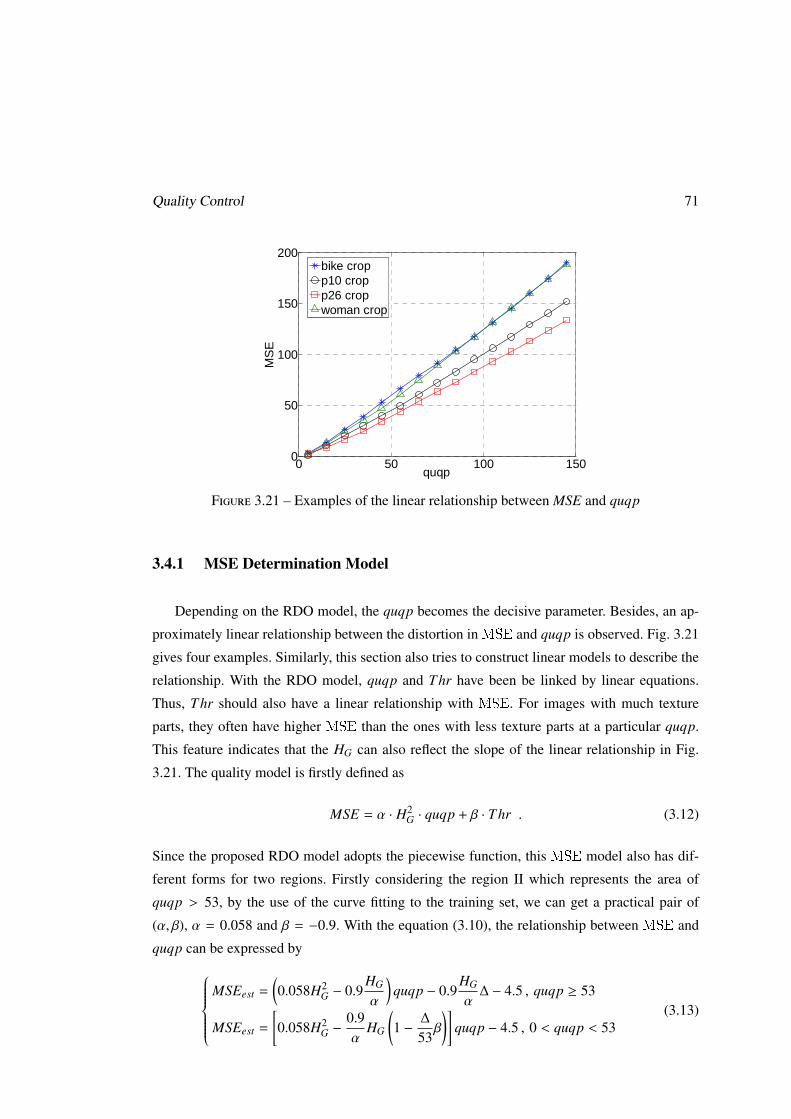
Quality Control 71
0 50 100 1500
50
100
150
200
quqp
MS
E
bike cropp10 cropp26 cropwoman crop
Figure 3.21 – Examples of the linear relationship between MSE and quqp
3.4.1 MSE Determination Model
Depending on the RDO model, the quqp becomes the decisive parameter. Besides, an ap-
proximately linear relationship between the distortion in MSE and quqp is observed. Fig. 3.21
gives four examples. Similarly, this section also tries to construct linear models to describe the
relationship. With the RDO model, quqp and Thr have been be linked by linear equations.
Thus, Thr should also have a linear relationship with MSE. For images with much texture
parts, they often have higher MSE than the ones with less texture parts at a particular quqp.
This feature indicates that the HG can also reflect the slope of the linear relationship in Fig.
3.21. The quality model is firstly defined as
MSE = α · H2G · quqp + β · Thr . (3.12)
Since the proposed RDO model adopts the piecewise function, this MSE model also has dif-
ferent forms for two regions. Firstly considering the region II which represents the area of
quqp > 53, by the use of the curve fitting to the training set, we can get a practical pair of
(α, β), α = 0.058 and β = −0.9. With the equation (3.10), the relationship between MSE and
quqp can be expressed byMSEest =
(0.058H2
G − 0.9HG
α
)quqp − 0.9
HG
α∆ − 4.5 , quqp ≥ 53
MSEest =
[0.058H2
G −0.9α
HG
(1 −
∆
53β
)]quqp − 4.5 , 0 < quqp < 53
(3.13)
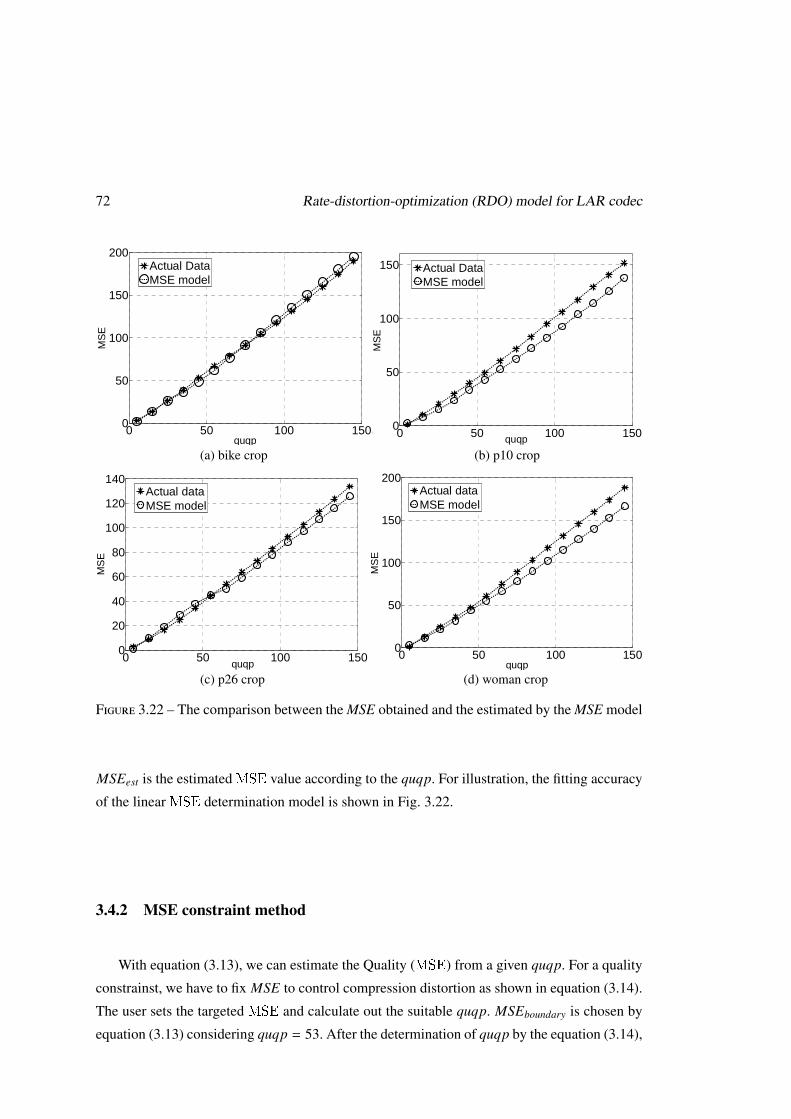
72 Rate-distortion-optimization (RDO) model for LAR codec
0 50 100 1500
50
100
150
200
quqp
MS
E
Actual DataMSE model
0 50 100 1500
50
100
150
quqp
MS
E
Actual DataMSE model
0 50 100 1500
20
40
60
80
100
120
140
quqp
MS
E
Actual dataMSE model
0 50 100 1500
50
100
150
200
quqp
MS
E
Actual dataMSE model
0 50 100 1500
50
100
150
200
quqp
MS
E
bike cropp10 cropp26 cropwoman crop
(a) bike crop
0 50 100 1500
50
100
150
200
quqp
MS
E
Actual DataMSE model
0 50 100 1500
50
100
150
quqp
MS
E
Actual DataMSE model
0 50 100 1500
20
40
60
80
100
120
140
quqp
MS
E
Actual dataMSE model
0 50 100 1500
50
100
150
200
quqp
MS
E
Actual dataMSE model
0 50 100 1500
50
100
150
200
quqp
MS
E
bike cropp10 cropp26 cropwoman crop
(b) p10 crop
0 50 100 1500
50
100
150
200
quqp
MS
E
Actual DataMSE model
0 50 100 1500
50
100
150
quqp
MS
E
Actual DataMSE model
0 50 100 1500
20
40
60
80
100
120
140
quqp
MS
E
Actual dataMSE model
0 50 100 1500
50
100
150
200
quqp
MS
E
Actual dataMSE model
0 50 100 1500
50
100
150
200
quqp
MS
E
bike cropp10 cropp26 cropwoman crop
(c) p26 crop
0 50 100 1500
50
100
150
200
quqp
MS
E
Actual DataMSE model
0 50 100 1500
50
100
150
quqp
MS
E
Actual DataMSE model
0 50 100 1500
20
40
60
80
100
120
140
quqp
MS
E
Actual dataMSE model
0 50 100 1500
50
100
150
200
quqp
MS
E
Actual dataMSE model
0 50 100 1500
50
100
150
200
quqp
MS
E
bike cropp10 cropp26 cropwoman crop
(d) woman crop
Figure 3.22 – The comparison between the MSE obtained and the estimated by the MSE model
MSEest is the estimated MSE value according to the quqp. For illustration, the fitting accuracy
of the linear MSE determination model is shown in Fig. 3.22.
3.4.2 MSE constraint method
With equation (3.13), we can estimate the Quality (MSE) from a given quqp. For a quality
constrainst, we have to fix MSE to control compression distortion as shown in equation (3.14).
The user sets the targeted MSE and calculate out the suitable quqp. MSEboundary is chosen by
equation (3.13) considering quqp = 53. After the determination of quqp by the equation (3.14),
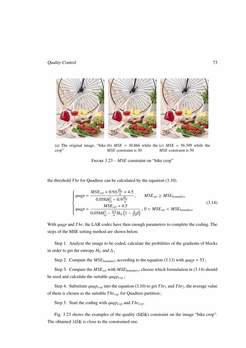
Quality Control 73
(a) The original image, “bikecrop”
(b) MSE = 30.866 while theMSE constraint is 30
(c) MSE = 56.399 while theMSE constraint is 50
Figure 3.23 – MSE constraint on “bike crop”
the threshold Thr for Quadtree can be calculated by the equation (3.10).
quqp =
MSEset + 0.9∆HGα + 4.5
0.058H2G − 0.9 HG
α
, MSEset ≥ MSEboundary
quqp =MSEset + 4.5
0.058H2G −
0.9α HG
(1 − ∆
53β) , 0 < MSEset < MSEboundary
(3.14)
With quqp and Thr, the LAR codec have then enough parameters to complete the coding. The
steps of the MSE setting method are shown below.
Step 1. Analyze the image to be coded, calculate the probilities of the gradients of blocks
in order to get the entropy HG and ∆ ;
Step 2. Compute the MSEboundary according to the equation (3.13) with quqp = 53 ;
Step 3. Compare the MSEset with MSEboundary, choose which formulation in (3.14) should
be used and calculate the suitable quqpexp ;
Step 4. Substitute quqpexp into the equation (3.10) to get Thr1 and Thr2, the average value
of them is chosen as the suitable Threxp for Quadtree partition ;
Step 5. Start the coding with quqpexp and Threxp.
Fig. 3.23 shows the examples of the quality (MSE) constraint on the image “bike crop”.
The obtained MSE is close to the constrained one.
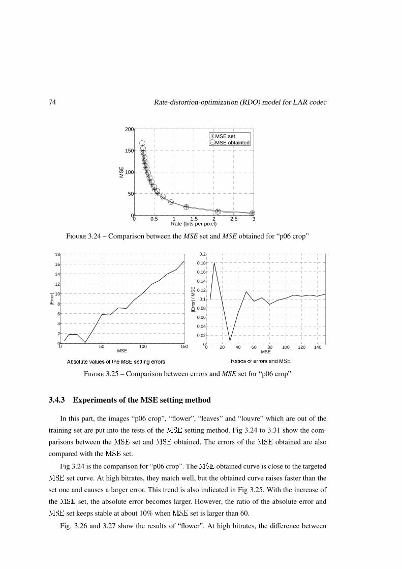
74 Rate-distortion-optimization (RDO) model for LAR codec
0 50 100 1500
50
100
150
200
quqp
MS
E
Actual Data
0 50 100 1500
20
40
60
80
100
120
140
quqp
MS
E
Actual data
0 50 100 1500
50
100
150
200
quqp
MS
E
Actual DataMSE model
0 50 100 1500
20
40
60
80
100
120
140
quqp
MS
E
Actual dataMSE model
0 0.5 1 1.5 2 2.5 30
50
100
150
200
Rate (bits per pixel)
MS
E
MSE setMSE obtainted
0.05 0.1 0.15 0.20
5
10
15
20
25
Rate (bits per pixel)
MS
E
MSE setMSE obtained
0 0.5 1 1.5 2
20
40
60
80
100
120
140
Rate (bite per pixel)
MS
E
MSE setMSE obtained
0 0.5 1 1.5 2 2.5 30
20
40
60
80
100
120
140
Rate (bits per pixel)
MS
E
MSE setMSE obtained
Figure 3.24 – Comparison between the MSE set and MSE obtained for “p06 crop”
0 20 40 60 80 100 120 1400
0.02
0.04
0.06
0.08
0.1
0.12
0.14
0.16
0.18
0.2
MSE
|Err
or| /
MS
E
0 50 100 1500
2
4
6
8
10
12
14
16
18
MSE
|Err
or|
p06 crop flower leaves louvre
0 5 10 15 20 252
2.5
3
3.5
4
4.5
5
5.5
MSE
|Err
or|
Absolute values of the MSE setting errors
0 5 10 15 20 250
1
2
3
4
5
6
MSE
|Err
or| /
MS
E
Ratios of errors and MSE
0 50 100 1500
1
2
3
4
5
6
7
MSE
|Err
or|
0 50 100 1500
0.02
0.04
0.06
0.08
0.1
0.12
0.14
MSE
|Err
or| /
MS
E
0 50 100 1500
1
2
3
4
5
6
MSE
|Err
or|
0 50 100 1500
0.05
0.1
0.15
0.2
0.25
MSE
|Err
or| /
MS
E
Figure 3.25 – Comparison between errors and MSE set for “p06 crop”
3.4.3 Experiments of the MSE setting method
In this part, the images “p06 crop”, “flower”, “leaves” and “louvre” which are out of the
training set are put into the tests of the MSE setting method. Fig 3.24 to 3.31 show the com-
parisons between the MSE set and MSE obtained. The errors of the MSE obtained are also
compared with the MSE set.
Fig 3.24 is the comparison for “p06 crop”. The MSE obtained curve is close to the targeted
MSE set curve. At high bitrates, they match well, but the obtained curve raises faster than the
set one and causes a larger error. This trend is also indicated in Fig 3.25. With the increase of
the MSE set, the absolute error becomes larger. However, the ratio of the absolute error and
MSE set keeps stable at about 10% when MSE set is larger than 60.
Fig. 3.26 and 3.27 show the results of “flower”. At high bitrates, the difference between
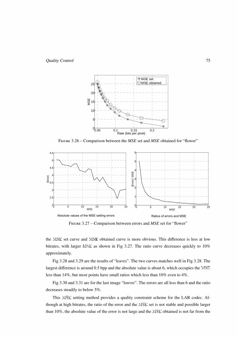
Quality Control 75
0 50 100 1500
50
100
150
200
quqp
MS
E
Actual Data
0 50 100 1500
20
40
60
80
100
120
140
quqp
MS
E
Actual data
0 50 100 1500
50
100
150
200
quqp
MS
E
Actual DataMSE model
0 50 100 1500
20
40
60
80
100
120
140
quqp
MS
E
Actual dataMSE model
0 0.5 1 1.5 2 2.5 30
50
100
150
200
Rate (bits per pixel)
MS
E
MSE setMSE obtainted
0.05 0.1 0.15 0.20
5
10
15
20
25
Rate (bits per pixel)
MS
E
MSE setMSE obtained
0 0.5 1 1.5 2
20
40
60
80
100
120
140
Rate (bite per pixel)
MS
E
MSE setMSE obtained
0 0.5 1 1.5 2 2.5 30
20
40
60
80
100
120
140
Rate (bits per pixel)
MS
E
MSE setMSE obtained
Figure 3.26 – Comparison between the MSE set and MSE obtained for “flower”
0 20 40 60 80 100 120 1400
0.02
0.04
0.06
0.08
0.1
0.12
0.14
0.16
0.18
0.2
MSE
|Err
or| /
MS
E
0 50 100 1500
2
4
6
8
10
12
14
16
18
MSE
|Err
or|
p06 crop flower leaves louvre
0 5 10 15 20 252
2.5
3
3.5
4
4.5
5
5.5
MSE
|Err
or|
Absolute values of the MSE setting errors
0 5 10 15 20 250
1
2
3
4
5
6
MSE
|Err
or| /
MS
E
Ratios of errors and MSE
0 50 100 1500
1
2
3
4
5
6
7
MSE
|Err
or|
0 50 100 1500
0.02
0.04
0.06
0.08
0.1
0.12
0.14
MSE
|Err
or| /
MS
E
0 50 100 1500
1
2
3
4
5
6
MSE
|Err
or|
0 50 100 1500
0.05
0.1
0.15
0.2
0.25
MSE
|Err
or| /
MS
E
Figure 3.27 – Comparison between errors and MSE set for “flower”
the MSE set curve and MSE obtained curve is more obvious. This difference is less at low
bitrates, with larger MSE as shown in Fig 3.27. The ratio curve decreases quickly to 10%
approximately.
Fig 3.28 and 3.29 are the results of “leaves”. The two curves matches well in Fig 3.28. The
largest difference is around 0.5 bpp and the absolute value is about 6, which occupies the MSE
less than 14%, but most points have small ratios which less than 10% even to 4%.
Fig 3.30 and 3.31 are for the last image “louvre”. The errors are all less than 6 and the ratio
decreases steadily to below 5%.
This MSE setting method provides a quality constraint scheme for the LAR codec. Al-
though at high bitrates, the ratio of the error and the MSE set is not stable and possible larger
than 10%, the absolute value of the error is not large and the MSE obtained is not far from the
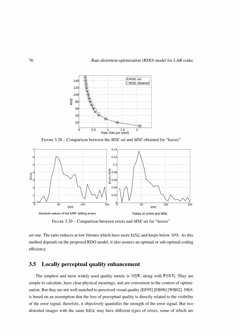
76 Rate-distortion-optimization (RDO) model for LAR codec
0 50 100 1500
50
100
150
200
quqp
MS
E
Actual Data
0 50 100 1500
20
40
60
80
100
120
140
quqp
MS
E
Actual data
0 50 100 1500
50
100
150
200
quqp
MS
E
Actual DataMSE model
0 50 100 1500
20
40
60
80
100
120
140
quqp
MS
E
Actual dataMSE model
0 0.5 1 1.5 2 2.5 30
50
100
150
200
Rate (bits per pixel)
MS
E
MSE setMSE obtainted
0.05 0.1 0.15 0.20
5
10
15
20
25
Rate (bits per pixel)
MS
E
MSE setMSE obtained
0 0.5 1 1.5 2
20
40
60
80
100
120
140
Rate (bite per pixel)
MS
E
MSE setMSE obtained
0 0.5 1 1.5 2 2.5 30
20
40
60
80
100
120
140
Rate (bits per pixel)
MS
E
MSE setMSE obtained
Figure 3.28 – Comparison between the MSE set and MSE obtained for “leaves”
0 20 40 60 80 100 120 1400
0.02
0.04
0.06
0.08
0.1
0.12
0.14
0.16
0.18
0.2
MSE
|Err
or| /
MS
E
0 50 100 1500
2
4
6
8
10
12
14
16
18
MSE
|Err
or|
p06 crop flower leaves louvre
0 5 10 15 20 252
2.5
3
3.5
4
4.5
5
5.5
MSE
|Err
or|
Absolute values of the MSE setting errors
0 5 10 15 20 250
1
2
3
4
5
6
MSE
|Err
or| /
MS
E
Ratios of errors and MSE
0 50 100 1500
1
2
3
4
5
6
7
MSE
|Err
or|
0 50 100 1500
0.02
0.04
0.06
0.08
0.1
0.12
0.14
MSE
|Err
or| /
MS
E
0 50 100 1500
1
2
3
4
5
6
MSE
|Err
or|
0 50 100 1500
0.05
0.1
0.15
0.2
0.25
MSE
|Err
or| /
MS
E
Figure 3.29 – Comparison between errors and MSE set for “leaves”
set one. The ratio reduces at low bitrates which have more MSE and keeps below 10%. As this
method depends on the proposed RDO model, it also assures an optimal or sub-optimal coding
efficiency.
3.5 Locally perceptual quality enhancement
The simplest and most widely used quality metric is MSE, along with PSNR. They are
simple to calculate, have clear physical meanings, and are convenient in the context of optimi-
zation. But they are not well matched to perceived visual quality [EF95] [EB98] [WB02]. MSE
is based on an assumption that the loss of perceptual quality is directly related to the visibility
of the error signal, therefore, it objectively quantifies the strength of the error signal. But two
distorted images with the same MSE may have different types of errors, some of which are
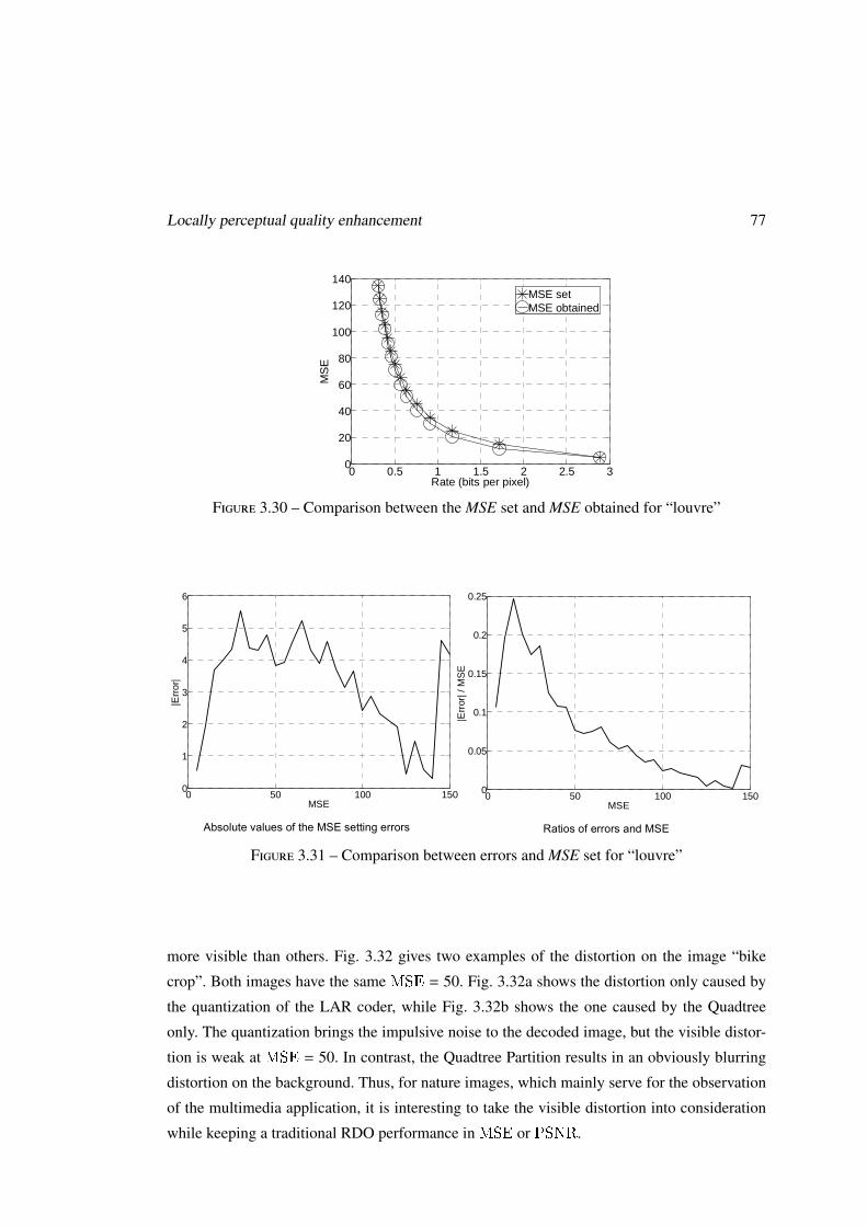
Locally perceptual quality enhancement 77
0 50 100 1500
50
100
150
200
quqp
MS
E
Actual Data
0 50 100 1500
20
40
60
80
100
120
140
quqp
MS
E
Actual data
0 50 100 1500
50
100
150
200
quqp
MS
E
Actual DataMSE model
0 50 100 1500
20
40
60
80
100
120
140
quqp
MS
E
Actual dataMSE model
0 0.5 1 1.5 2 2.5 30
50
100
150
200
Rate (bits per pixel)
MS
E
MSE setMSE obtainted
0.05 0.1 0.15 0.20
5
10
15
20
25
Rate (bits per pixel)
MS
E
MSE setMSE obtained
0 0.5 1 1.5 2
20
40
60
80
100
120
140
Rate (bite per pixel)
MS
E
MSE setMSE obtained
0 0.5 1 1.5 2 2.5 30
20
40
60
80
100
120
140
Rate (bits per pixel)
MS
E
MSE setMSE obtained
Figure 3.30 – Comparison between the MSE set and MSE obtained for “louvre”
0 20 40 60 80 100 120 1400
0.02
0.04
0.06
0.08
0.1
0.12
0.14
0.16
0.18
0.2
MSE
|Err
or| /
MS
E
0 50 100 1500
2
4
6
8
10
12
14
16
18
MSE
|Err
or|
p06 crop flower leaves louvre
0 5 10 15 20 252
2.5
3
3.5
4
4.5
5
5.5
MSE
|Err
or|
0 5 10 15 20 250
1
2
3
4
5
6
MSE
|Err
or| /
MS
E
0 50 100 1500
1
2
3
4
5
6
7
MSE
|Err
or|
0 50 100 1500
0.02
0.04
0.06
0.08
0.1
0.12
0.14
MSE
|Err
or| /
MS
E
0 50 100 1500
1
2
3
4
5
6
MSE
|Err
or|
Absolute values of the MSE setting errors
0 50 100 1500
0.05
0.1
0.15
0.2
0.25
MSE
|Err
or| /
MS
E
Ratios of errors and MSE Figure 3.31 – Comparison between errors and MSE set for “louvre”
more visible than others. Fig. 3.32 gives two examples of the distortion on the image “bike
crop”. Both images have the same MSE = 50. Fig. 3.32a shows the distortion only caused by
the quantization of the LAR coder, while Fig. 3.32b shows the one caused by the Quadtree
only. The quantization brings the impulsive noise to the decoded image, but the visible distor-
tion is weak at MSE = 50. In contrast, the Quadtree Partition results in an obviously blurring
distortion on the background. Thus, for nature images, which mainly serve for the observation
of the multimedia application, it is interesting to take the visible distortion into consideration
while keeping a traditional RDO performance in MSE or PSNR.
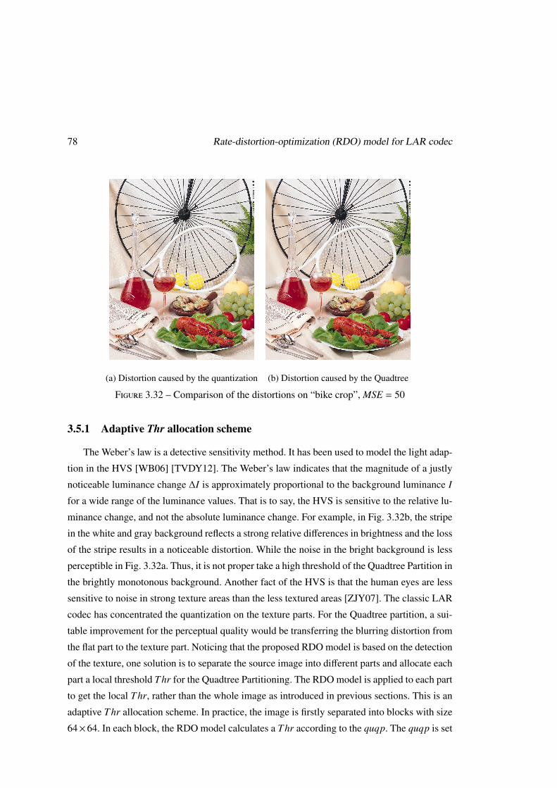
78 Rate-distortion-optimization (RDO) model for LAR codec
(a) Distortion caused by the quantization (b) Distortion caused by the Quadtree
Figure 3.32 – Comparison of the distortions on “bike crop”, MSE = 50
3.5.1 Adaptive Thr allocation scheme
The Weber’s law is a detective sensitivity method. It has been used to model the light adap-
tion in the HVS [WB06] [TVDY12]. The Weber’s law indicates that the magnitude of a justly
noticeable luminance change ∆I is approximately proportional to the background luminance I
for a wide range of the luminance values. That is to say, the HVS is sensitive to the relative lu-
minance change, and not the absolute luminance change. For example, in Fig. 3.32b, the stripe
in the white and gray background reflects a strong relative differences in brightness and the loss
of the stripe results in a noticeable distortion. While the noise in the bright background is less
perceptible in Fig. 3.32a. Thus, it is not proper take a high threshold of the Quadtree Partition in
the brightly monotonous background. Another fact of the HVS is that the human eyes are less
sensitive to noise in strong texture areas than the less textured areas [ZJY07]. The classic LAR
codec has concentrated the quantization on the texture parts. For the Quadtree partition, a sui-
table improvement for the perceptual quality would be transferring the blurring distortion from
the flat part to the texture part. Noticing that the proposed RDO model is based on the detection
of the texture, one solution is to separate the source image into different parts and allocate each
part a local threshold Thr for the Quadtree Partitioning. The RDO model is applied to each part
to get the local Thr, rather than the whole image as introduced in previous sections. This is an
adaptive Thr allocation scheme. In practice, the image is firstly separated into blocks with size
64×64. In each block, the RDO model calculates a Thr according to the quqp. The quqp is set
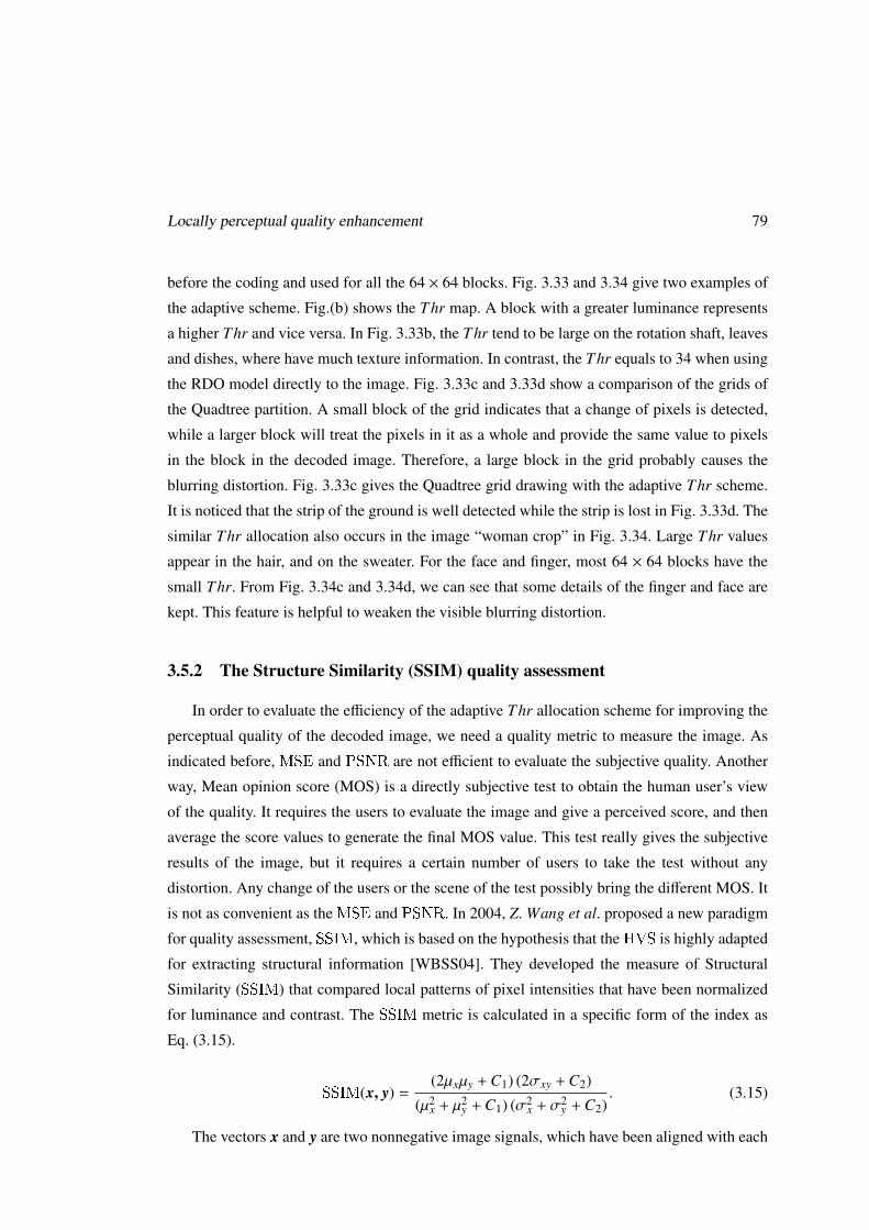
Locally perceptual quality enhancement 79
before the coding and used for all the 64 × 64 blocks. Fig. 3.33 and 3.34 give two examples of
the adaptive scheme. Fig.(b) shows the Thr map. A block with a greater luminance represents
a higher Thr and vice versa. In Fig. 3.33b, the Thr tend to be large on the rotation shaft, leaves
and dishes, where have much texture information. In contrast, the Thr equals to 34 when using
the RDO model directly to the image. Fig. 3.33c and 3.33d show a comparison of the grids of
the Quadtree partition. A small block of the grid indicates that a change of pixels is detected,
while a larger block will treat the pixels in it as a whole and provide the same value to pixels
in the block in the decoded image. Therefore, a large block in the grid probably causes the
blurring distortion. Fig. 3.33c gives the Quadtree grid drawing with the adaptive Thr scheme.
It is noticed that the strip of the ground is well detected while the strip is lost in Fig. 3.33d. The
similar Thr allocation also occurs in the image “woman crop” in Fig. 3.34. Large Thr values
appear in the hair, and on the sweater. For the face and finger, most 64 × 64 blocks have the
small Thr. From Fig. 3.34c and 3.34d, we can see that some details of the finger and face are
kept. This feature is helpful to weaken the visible blurring distortion.
3.5.2 The Structure Similarity (SSIM) quality assessment
In order to evaluate the efficiency of the adaptive Thr allocation scheme for improving the
perceptual quality of the decoded image, we need a quality metric to measure the image. As
indicated before, MSE and PSNR are not efficient to evaluate the subjective quality. Another
way, Mean opinion score (MOS) is a directly subjective test to obtain the human user’s view
of the quality. It requires the users to evaluate the image and give a perceived score, and then
average the score values to generate the final MOS value. This test really gives the subjective
results of the image, but it requires a certain number of users to take the test without any
distortion. Any change of the users or the scene of the test possibly bring the different MOS. It
is not as convenient as the MSE and PSNR. In 2004, Z. Wang et al. proposed a new paradigm
for quality assessment, SSIM, which is based on the hypothesis that the HVS is highly adapted
for extracting structural information [WBSS04]. They developed the measure of Structural
Similarity (SSIM) that compared local patterns of pixel intensities that have been normalized
for luminance and contrast. The SSIM metric is calculated in a specific form of the index as
Eq. (3.15).
SSIM(x, y) =(2µxµy + C1) (2σxy + C2)
(µ2x + µ2
y + C1) (σ2x + σ2
y + C2). (3.15)
The vectors x and y are two nonnegative image signals, which have been aligned with each
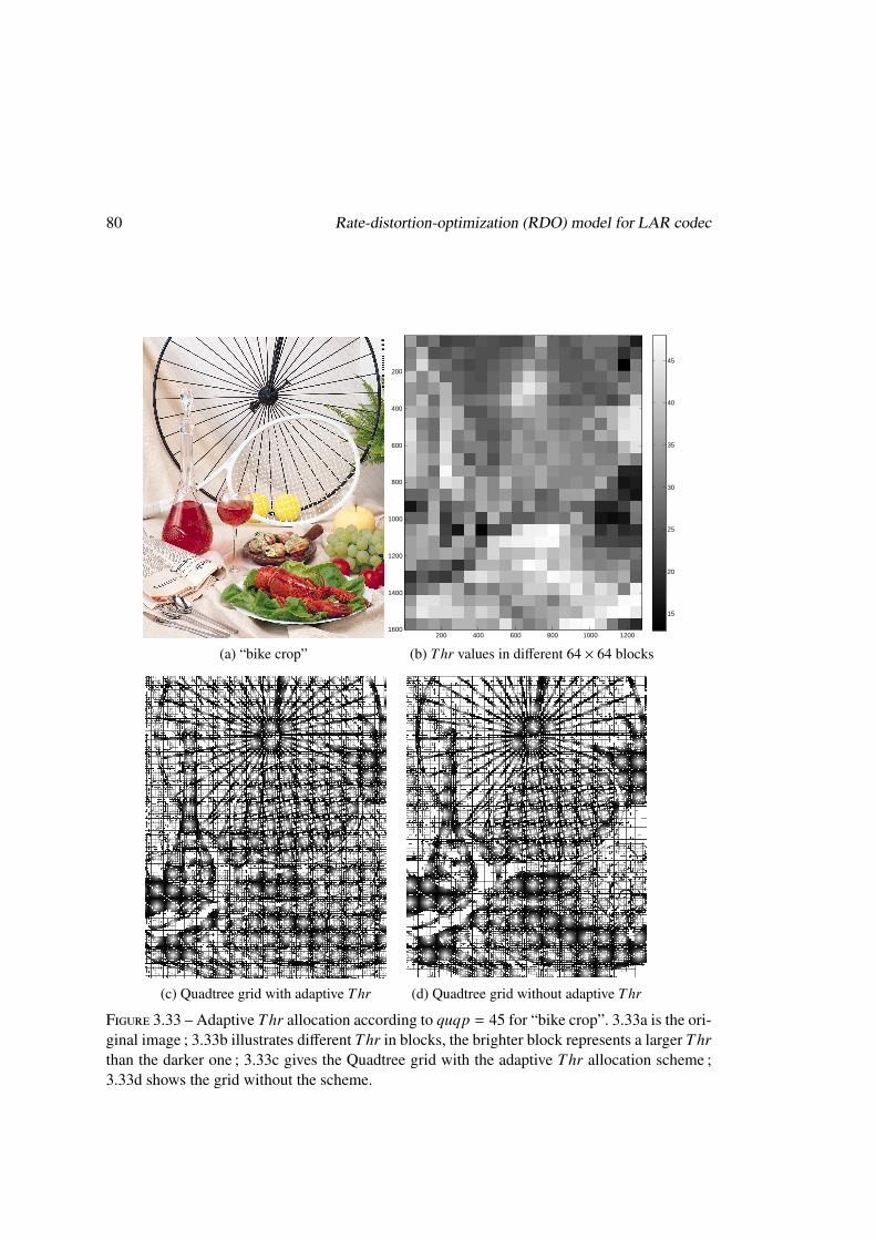
80 Rate-distortion-optimization (RDO) model for LAR codec
(a) “bike crop”
200 400 600 800 1000 1200
200
400
600
800
1000
1200
1400
1600
15
20
25
30
35
40
45
(b) Thr values in different 64 × 64 blocks
(c) Quadtree grid with adaptive Thr (d) Quadtree grid without adaptive Thr
Figure 3.33 – Adaptive Thr allocation according to quqp = 45 for “bike crop”. 3.33a is the ori-ginal image ; 3.33b illustrates different Thr in blocks, the brighter block represents a larger Thrthan the darker one ; 3.33c gives the Quadtree grid with the adaptive Thr allocation scheme ;3.33d shows the grid without the scheme.
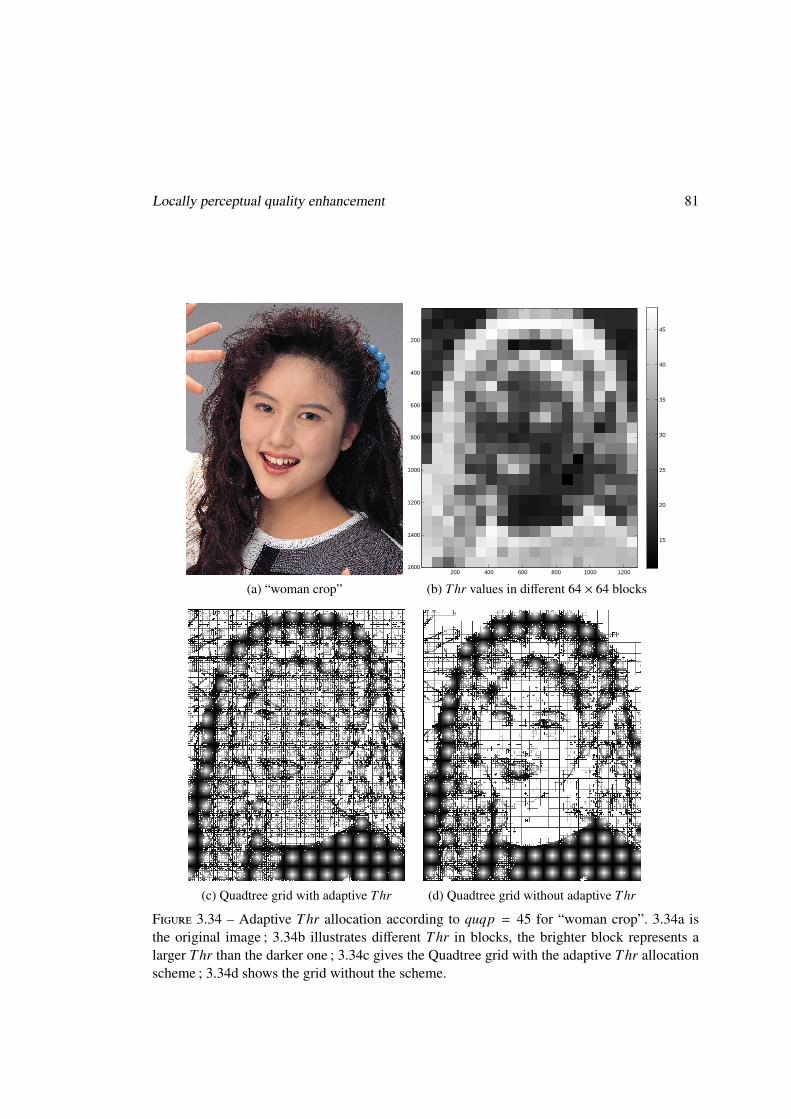
Locally perceptual quality enhancement 81
(a) “woman crop”
200 400 600 800 1000 1200
200
400
600
800
1000
1200
1400
1600
15
20
25
30
35
40
45
(b) Thr values in different 64 × 64 blocks
(c) Quadtree grid with adaptive Thr (d) Quadtree grid without adaptive Thr
Figure 3.34 – Adaptive Thr allocation according to quqp = 45 for “woman crop”. 3.34a isthe original image ; 3.34b illustrates different Thr in blocks, the brighter block represents alarger Thr than the darker one ; 3.34c gives the Quadtree grid with the adaptive Thr allocationscheme ; 3.34d shows the grid without the scheme.
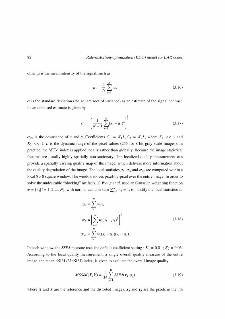
82 Rate-distortion-optimization (RDO) model for LAR codec
other. µ is the mean intensity of the signal, such as
µx =1N
N∑i=1
xi. (3.16)
σ is the standard deviation (the square root of variance) as an estimate of the signal contrast.
Its an unbiased estimate is given by
σx =
1N − 1
N∑i=1
(xi − µx)2
12
(3.17)
σxy is the covariance of x and y. Coefficients C1 = K1L,C2 = K2L, where K1 << 1 and
K2 << 1. L is the dynamic range of the pixel-values (255 for 8-bit gray scale images). In
practice, the SSIM index is applied locally rather than globally. Because the image statistical
features are usually highly spatially non-stationary. The localized quality measurement can
provide a spatially varying quality map of the image, which delivers more information about
the quality degradation of the image. The local statistics µx, σx and σxy are computed within a
local 8×8 square window. The window moves pixel-by-pixel over the entire image. In order to
solve the undesirable “blocking” artifacts, Z. Wang et al. used an Gaussian weighting function
w = {wi| i = 1, 2, ...,N}, with normalized unit sum∑N
i=1 wi = 1, to modify the local statistics as
µx =
N∑i=1
wixi
σx =
N∑i=1
wi(xi − µx)2
12
σxy =
N∑i=1
wi(xi − µx)(yi − µy).
(3.18)
In each window, the SSIM measure uses the default coefficient setting : K1 = 0.01 ; K2 = 0.03.
According to the local quality measurement, a single overall quality measure of the entire
image, the mean SSIM (MSSIM) index, is given to evaluate the overall image quality
MSSIM(X, Y) =1M
M∑j=1
SSIM(x j, y j) (3.19)
where X and Y are the reference and the distorted images. x j and y j are the pixels in the jth
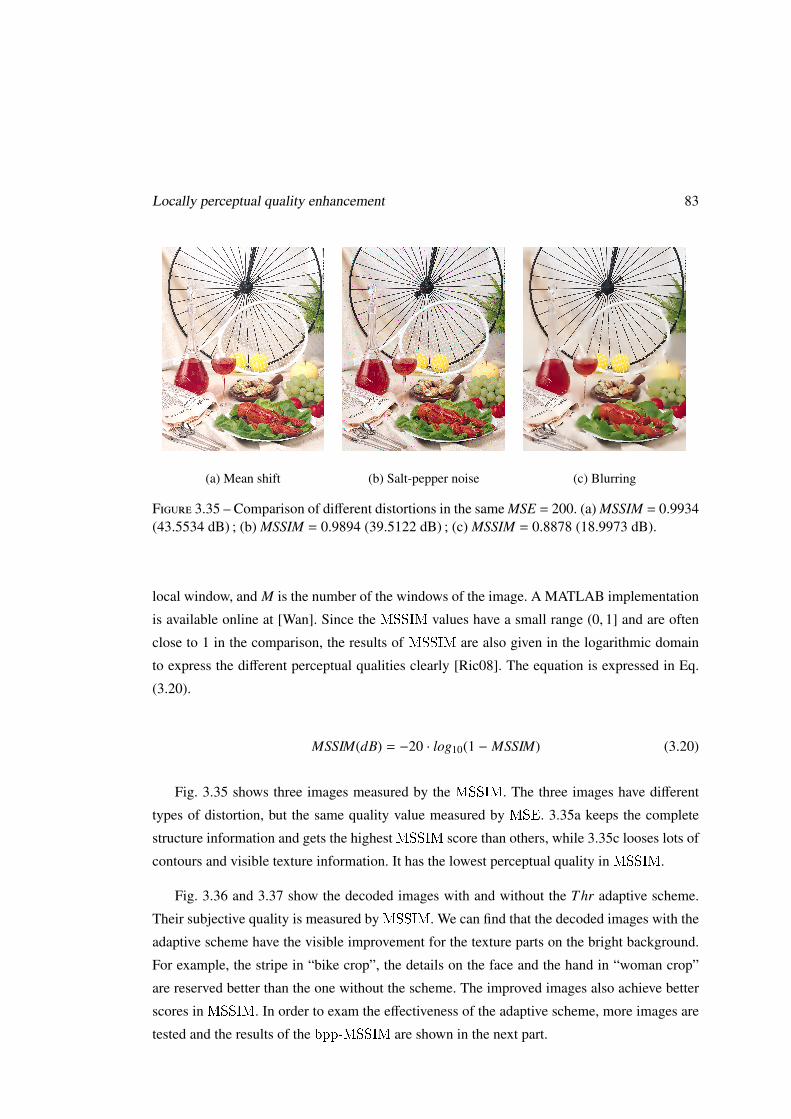
Locally perceptual quality enhancement 83
(a) Mean shift (b) Salt-pepper noise (c) Blurring
Figure 3.35 – Comparison of different distortions in the same MSE = 200. (a) MSSIM = 0.9934(43.5534 dB) ; (b) MSSIM = 0.9894 (39.5122 dB) ; (c) MSSIM = 0.8878 (18.9973 dB).
local window, and M is the number of the windows of the image. A MATLAB implementation
is available online at [Wan]. Since the MSSIM values have a small range (0, 1] and are often
close to 1 in the comparison, the results of MSSIM are also given in the logarithmic domain
to express the different perceptual qualities clearly [Ric08]. The equation is expressed in Eq.
(3.20).
MSSIM(dB) = −20 · log10(1 − MSSIM) (3.20)
Fig. 3.35 shows three images measured by the MSSIM. The three images have different
types of distortion, but the same quality value measured by MSE. 3.35a keeps the complete
structure information and gets the highest MSSIM score than others, while 3.35c looses lots of
contours and visible texture information. It has the lowest perceptual quality in MSSIM.
Fig. 3.36 and 3.37 show the decoded images with and without the Thr adaptive scheme.
Their subjective quality is measured by MSSIM. We can find that the decoded images with the
adaptive scheme have the visible improvement for the texture parts on the bright background.
For example, the stripe in “bike crop”, the details on the face and the hand in “woman crop”
are reserved better than the one without the scheme. The improved images also achieve better
scores in MSSIM. In order to exam the effectiveness of the adaptive scheme, more images are
tested and the results of the bpp-MSSIM are shown in the next part.
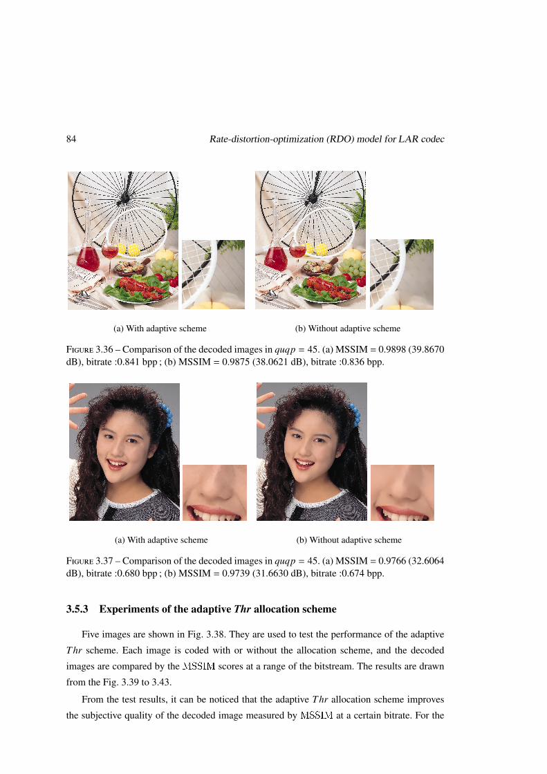
84 Rate-distortion-optimization (RDO) model for LAR codec
(a) With adaptive scheme
(b) Without adaptive scheme
Figure 3.36 – Comparison of the decoded images in quqp = 45. (a) MSSIM = 0.9898 (39.8670dB), bitrate :0.841 bpp ; (b) MSSIM = 0.9875 (38.0621 dB), bitrate :0.836 bpp.
(a) With adaptive scheme
(b) Without adaptive scheme
Figure 3.37 – Comparison of the decoded images in quqp = 45. (a) MSSIM = 0.9766 (32.6064dB), bitrate :0.680 bpp ; (b) MSSIM = 0.9739 (31.6630 dB), bitrate :0.674 bpp.
3.5.3 Experiments of the adaptive Thr allocation scheme
Five images are shown in Fig. 3.38. They are used to test the performance of the adaptive
Thr scheme. Each image is coded with or without the allocation scheme, and the decoded
images are compared by the MSSIM scores at a range of the bitstream. The results are drawn
from the Fig. 3.39 to 3.43.
From the test results, it can be noticed that the adaptive Thr allocation scheme improves
the subjective quality of the decoded image measured by MSSIM at a certain bitrate. For the
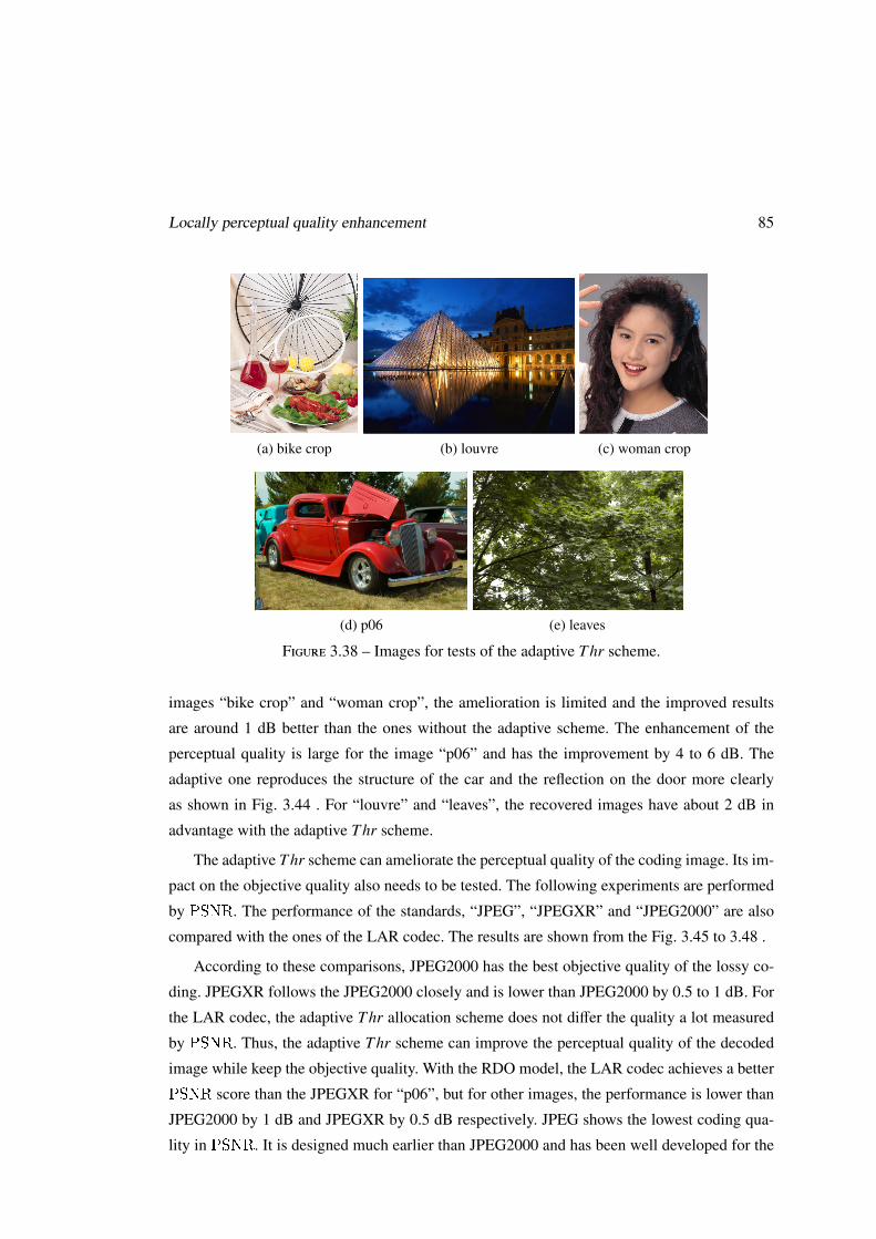
Locally perceptual quality enhancement 85
Leaves
Louvre
0 0.5 1 1.5 225
30
35
40
45
50
55
60
65
70
bpp
MS
SIM
(dB
)
with adaptive schemewithout adaptive scheme
0.3 0.4 0.5 0.6 0.7
38
40
42
44
46
48
bpp
MS
SIM
(dB
)
with adaptive schemewithout adaptive scheme
0 0.5 1 1.5 220
25
30
35
40
45
50
bpp
MS
SIM
(dB
)
with adaptive schemewithout adaptive scheme
0.3 0.4 0.5 0.6 0.7
28
29
30
31
32
33
34
bpp
MS
SIM
(dB
)
with adaptive schemewithout adaptive scheme
(a) bike crop
Leaves
Louvre
0 0.5 1 1.5 225
30
35
40
45
50
55
60
65
70
bpp
MS
SIM
(dB
)
with adaptive schemewithout adaptive scheme
0.3 0.4 0.5 0.6 0.7
38
40
42
44
46
48
bpp
MS
SIM
(dB
)
with adaptive schemewithout adaptive scheme
0 0.5 1 1.5 220
25
30
35
40
45
50
bpp
MS
SIM
(dB
)
with adaptive schemewithout adaptive scheme
0.3 0.4 0.5 0.6 0.7
28
29
30
31
32
33
34
bpp
MS
SIM
(dB
)
with adaptive schemewithout adaptive scheme
(b) louvre
Leaves
Louvre
0 0.5 1 1.5 225
30
35
40
45
50
55
60
65
70
bpp
MS
SIM
(dB
)
with adaptive schemewithout adaptive scheme
0.3 0.4 0.5 0.6 0.7
38
40
42
44
46
48
bpp
MS
SIM
(dB
)
with adaptive schemewithout adaptive scheme
0 0.5 1 1.5 220
25
30
35
40
45
50
bpp
MS
SIM
(dB
)
with adaptive schemewithout adaptive scheme
0.3 0.4 0.5 0.6 0.7
28
29
30
31
32
33
34
bpp
MS
SIM
(dB
)
with adaptive schemewithout adaptive scheme
(c) woman crop
Leaves
Louvre
0 0.5 1 1.5 225
30
35
40
45
50
55
60
65
70
bppM
SS
IM (
dB)
with adaptive schemewithout adaptive scheme
0.3 0.4 0.5 0.6 0.7
38
40
42
44
46
48
bpp
MS
SIM
(dB
)
with adaptive schemewithout adaptive scheme
0 0.5 1 1.5 220
25
30
35
40
45
50
bpp
MS
SIM
(dB
)
with adaptive schemewithout adaptive scheme
0.3 0.4 0.5 0.6 0.7
28
29
30
31
32
33
34
bpp
MS
SIM
(dB
)
with adaptive schemewithout adaptive scheme
(d) p06
Leaves
Louvre
0 0.5 1 1.5 225
30
35
40
45
50
55
60
65
70
bpp
MS
SIM
(dB
)
with adaptive schemewithout adaptive scheme
0.3 0.4 0.5 0.6 0.7
38
40
42
44
46
48
bpp
MS
SIM
(dB
)
with adaptive schemewithout adaptive scheme
0 0.5 1 1.5 220
25
30
35
40
45
50
bpp
MS
SIM
(dB
)
with adaptive schemewithout adaptive scheme
0.3 0.4 0.5 0.6 0.7
28
29
30
31
32
33
34
bpp
MS
SIM
(dB
)
with adaptive schemewithout adaptive scheme
(e) leaves
Figure 3.38 – Images for tests of the adaptive Thr scheme.
images “bike crop” and “woman crop”, the amelioration is limited and the improved results
are around 1 dB better than the ones without the adaptive scheme. The enhancement of the
perceptual quality is large for the image “p06” and has the improvement by 4 to 6 dB. The
adaptive one reproduces the structure of the car and the reflection on the door more clearly
as shown in Fig. 3.44 . For “louvre” and “leaves”, the recovered images have about 2 dB in
advantage with the adaptive Thr scheme.
The adaptive Thr scheme can ameliorate the perceptual quality of the coding image. Its im-
pact on the objective quality also needs to be tested. The following experiments are performed
by PSNR. The performance of the standards, “JPEG”, “JPEGXR” and “JPEG2000” are also
compared with the ones of the LAR codec. The results are shown from the Fig. 3.45 to 3.48 .
According to these comparisons, JPEG2000 has the best objective quality of the lossy co-
ding. JPEGXR follows the JPEG2000 closely and is lower than JPEG2000 by 0.5 to 1 dB. For
the LAR codec, the adaptive Thr allocation scheme does not differ the quality a lot measured
by PSNR. Thus, the adaptive Thr scheme can improve the perceptual quality of the decoded
image while keep the objective quality. With the RDO model, the LAR codec achieves a better
PSNR score than the JPEGXR for “p06”, but for other images, the performance is lower than
JPEG2000 by 1 dB and JPEGXR by 0.5 dB respectively. JPEG shows the lowest coding qua-
lity in PSNR. It is designed much earlier than JPEG2000 and has been well developed for the
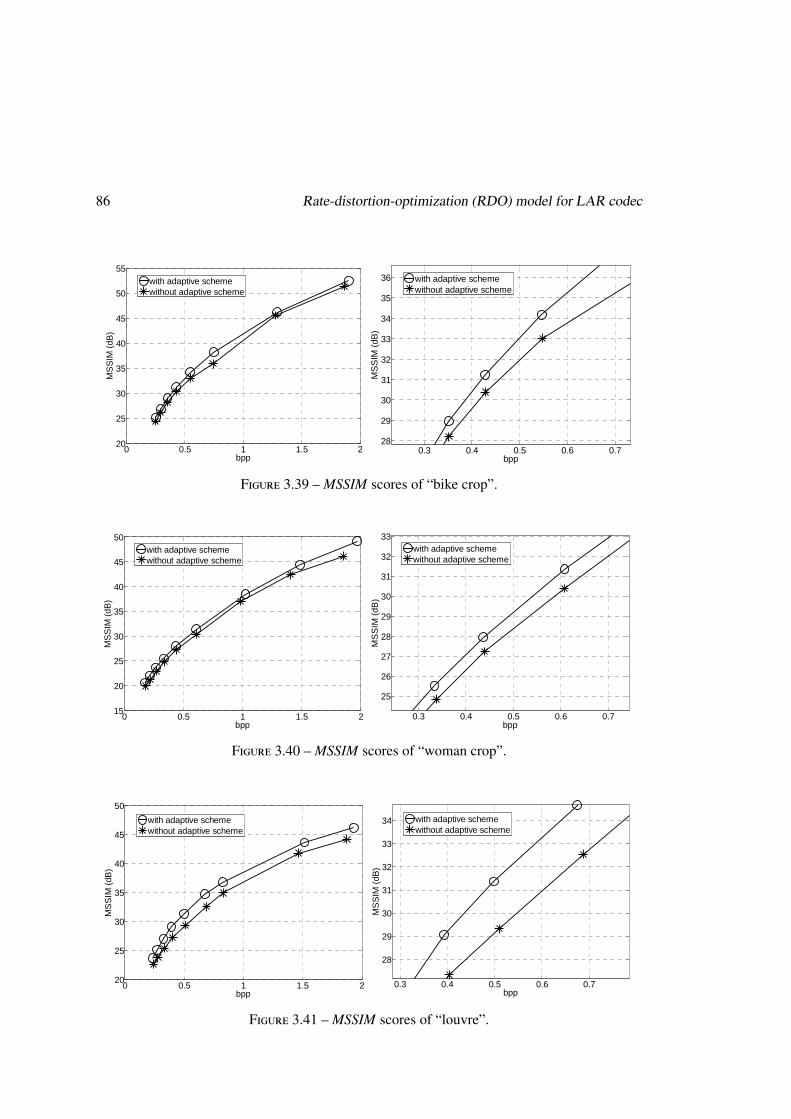
86 Rate-distortion-optimization (RDO) model for LAR codec
Bike crop
Woman crop
P06
0 0.5 1 1.5 220
25
30
35
40
45
50
55
bpp
MS
SIM
(dB
)
with adaptive schemewithout adaptive scheme
0.3 0.4 0.5 0.6 0.728
29
30
31
32
33
34
35
36
bpp
MS
SIM
(dB
)
with adaptive schemewithout adaptive scheme
0 0.5 1 1.5 215
20
25
30
35
40
45
50
bpp
MS
SIM
(dB
)
with adaptive schemewithout adaptive scheme
0.3 0.4 0.5 0.6 0.7
25
26
27
28
29
30
31
32
33
bpp
MS
SIM
(dB
)
with adaptive schemewithout adaptive scheme
0 0.5 1 1.5 220
25
30
35
40
45
50
55
60
65
bpp
MS
SIM
(dB
)
with adaptive scheme without adaptive scheme
0.3 0.4 0.5 0.6 0.7
36
38
40
42
44
46
bpp
MS
SIM
(dB
)
with adaptive scheme without adaptive scheme
Figure 3.39 – MSSIM scores of “bike crop”.
Bike crop
Woman crop
P06
0 0.5 1 1.5 220
25
30
35
40
45
50
55
bpp
MS
SIM
(dB
)
with adaptive schemewithout adaptive scheme
0.3 0.4 0.5 0.6 0.728
29
30
31
32
33
34
35
36
bpp
MS
SIM
(dB
)
with adaptive schemewithout adaptive scheme
0 0.5 1 1.5 215
20
25
30
35
40
45
50
bpp
MS
SIM
(dB
)
with adaptive schemewithout adaptive scheme
0.3 0.4 0.5 0.6 0.7
25
26
27
28
29
30
31
32
33
bpp
MS
SIM
(dB
)
with adaptive schemewithout adaptive scheme
0 0.5 1 1.5 220
25
30
35
40
45
50
55
60
65
bpp
MS
SIM
(dB
)
with adaptive scheme without adaptive scheme
0.3 0.4 0.5 0.6 0.7
36
38
40
42
44
46
bpp
MS
SIM
(dB
)
with adaptive scheme without adaptive scheme
Figure 3.40 – MSSIM scores of “woman crop”.
Leaves
louvre
0 0.5 1 1.5 225
30
35
40
45
50
55
60
65
70
bpp
MS
SIM
(dB
)
with adaptive schemewithout adaptive scheme
0.3 0.4 0.5 0.6 0.7
38
40
42
44
46
48
bpp
MS
SIM
(dB
)
with adaptive schemewithout adaptive scheme
0 0.5 1 1.5 220
25
30
35
40
45
50
bpp
MS
SIM
(dB
)
with adaptive schemewithout adaptive scheme
0.3 0.4 0.5 0.6 0.7
28
29
30
31
32
33
34
bpp
MS
SIM
(dB
)
with adaptive schemewithout adaptive scheme
Figure 3.41 – MSSIM scores of “louvre”.
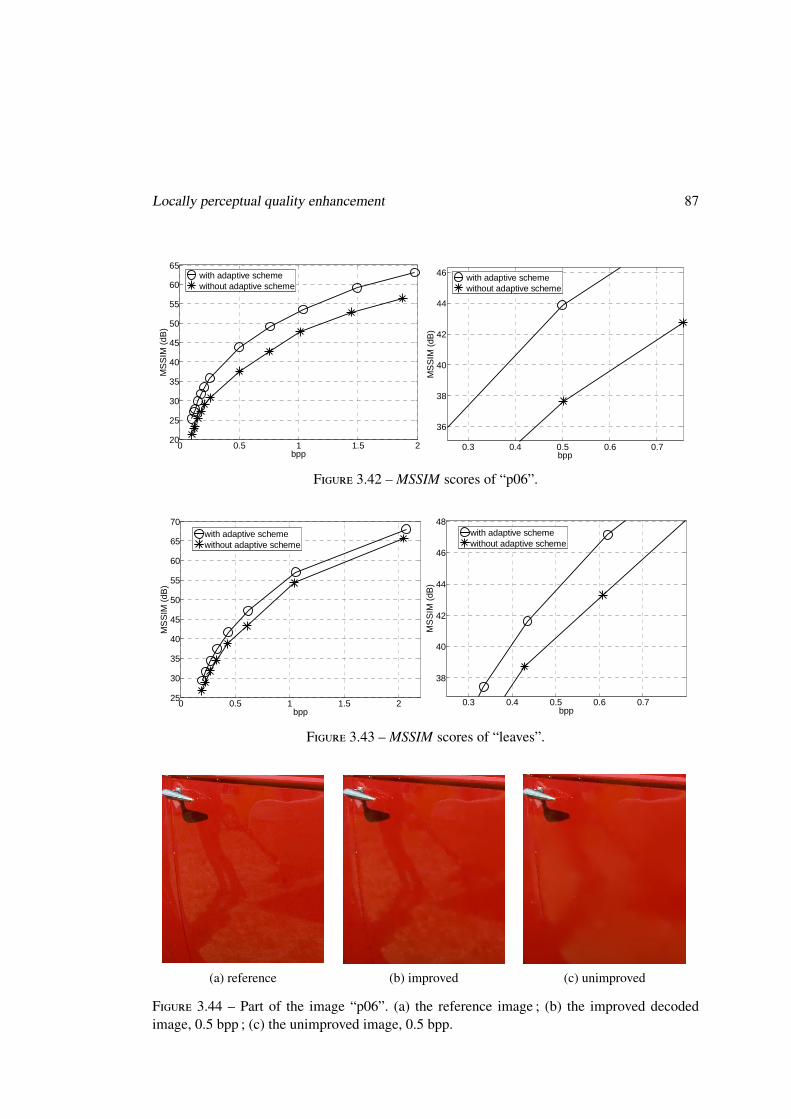
Locally perceptual quality enhancement 87
Bike crop
Woman crop
P06
0 0.5 1 1.5 220
25
30
35
40
45
50
55
bpp
MS
SIM
(dB
)
with adaptive schemewithout adaptive scheme
0.3 0.4 0.5 0.6 0.728
29
30
31
32
33
34
35
36
bpp
MS
SIM
(dB
)
with adaptive schemewithout adaptive scheme
0 0.5 1 1.5 215
20
25
30
35
40
45
50
bpp
MS
SIM
(dB
)
with adaptive schemewithout adaptive scheme
0.3 0.4 0.5 0.6 0.7
25
26
27
28
29
30
31
32
33
bpp
MS
SIM
(dB
)
with adaptive schemewithout adaptive scheme
0 0.5 1 1.5 220
25
30
35
40
45
50
55
60
65
bpp
MS
SIM
(dB
)
with adaptive scheme without adaptive scheme
0.3 0.4 0.5 0.6 0.7
36
38
40
42
44
46
bppM
SS
IM (
dB)
with adaptive scheme without adaptive scheme
Bike crop
Woman crop
P06
0 0.5 1 1.5 220
25
30
35
40
45
50
55
bpp
MS
SIM
(dB
)
with adaptive schemewithout adaptive scheme
0.3 0.4 0.5 0.6 0.728
29
30
31
32
33
34
35
36
bpp
MS
SIM
(dB
)
with adaptive schemewithout adaptive scheme
0 0.5 1 1.5 215
20
25
30
35
40
45
50
bpp
MS
SIM
(dB
)
with adaptive schemewithout adaptive scheme
0.3 0.4 0.5 0.6 0.7
25
26
27
28
29
30
31
32
33
bpp
MS
SIM
(dB
)
with adaptive schemewithout adaptive scheme
0 0.5 1 1.5 220
25
30
35
40
45
50
55
60
65
bpp
MS
SIM
(dB
)
with adaptive scheme without adaptive scheme
0.3 0.4 0.5 0.6 0.7
36
38
40
42
44
46
bpp
MS
SIM
(dB
)
with adaptive scheme without adaptive scheme
Figure 3.42 – MSSIM scores of “p06”.
Leaves
louvre
0 0.5 1 1.5 225
30
35
40
45
50
55
60
65
70
bpp
MS
SIM
(dB
)
with adaptive schemewithout adaptive scheme
0.3 0.4 0.5 0.6 0.7
38
40
42
44
46
48
bpp
MS
SIM
(dB
)
with adaptive schemewithout adaptive scheme
0 0.5 1 1.5 220
25
30
35
40
45
50
bpp
MS
SIM
(dB
)
with adaptive schemewithout adaptive scheme
0.3 0.4 0.5 0.6 0.7
28
29
30
31
32
33
34
bpp
MS
SIM
(dB
)
with adaptive schemewithout adaptive scheme
Figure 3.43 – MSSIM scores of “leaves”.
(a) reference
(b) improved
(c) unimproved
Figure 3.44 – Part of the image “p06”. (a) the reference image ; (b) the improved decodedimage, 0.5 bpp ; (c) the unimproved image, 0.5 bpp.
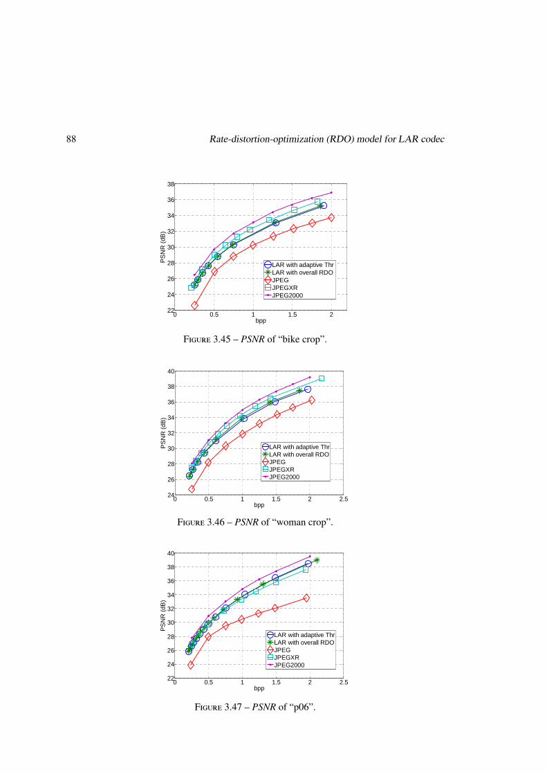
88 Rate-distortion-optimization (RDO) model for LAR codec
Bike crop
Woman crop
P06
0 0.5 1 1.5 222
24
26
28
30
32
34
36
38
bpp
PS
NR
(dB
)
LAR with adaptive ThrLAR with overall RDOJPEGJPEGXRJPEG2000
0 0.5 1 1.5 2 2.524
26
28
30
32
34
36
38
40
bpp
PS
NR
(dB
)
LAR with adaptive ThrLAR with overall RDOJPEGJPEGXRJPEG2000
0 0.5 1 1.5 2 2.522
24
26
28
30
32
34
36
38
40
bpp
PS
NR
(dB
)
LAR with adaptive ThrLAR with overall RDOJPEGJPEGXRJPEG2000
Figure 3.45 – PSNR of “bike crop”.
Bike crop
Woman crop
P06
0 0.5 1 1.5 222
24
26
28
30
32
34
36
38
bpp
PS
NR
(dB
)
LAR with adaptive ThrLAR with overall RDOJPEGJPEGXRJPEG2000
0 0.5 1 1.5 2 2.524
26
28
30
32
34
36
38
40
bpp
PS
NR
(dB
)
LAR with adaptive ThrLAR with overall RDOJPEGJPEGXRJPEG2000
0 0.5 1 1.5 2 2.522
24
26
28
30
32
34
36
38
40
bpp
PS
NR
(dB
)
LAR with adaptive ThrLAR with overall RDOJPEGJPEGXRJPEG2000
Figure 3.46 – PSNR of “woman crop”.
Bike crop
Woman crop
P06
0 0.5 1 1.5 222
24
26
28
30
32
34
36
38
bpp
PS
NR
(dB
)
LAR with adaptive ThrLAR with overall RDOJPEGJPEGXRJPEG2000
0 0.5 1 1.5 2 2.524
26
28
30
32
34
36
38
40
bpp
PS
NR
(dB
)
LAR with adaptive ThrLAR with overall RDOJPEGJPEGXRJPEG2000
0 0.5 1 1.5 2 2.522
24
26
28
30
32
34
36
38
40
bpp
PS
NR
(dB
)
LAR with adaptive ThrLAR with overall RDOJPEGJPEGXRJPEG2000
Figure 3.47 – PSNR of “p06”.
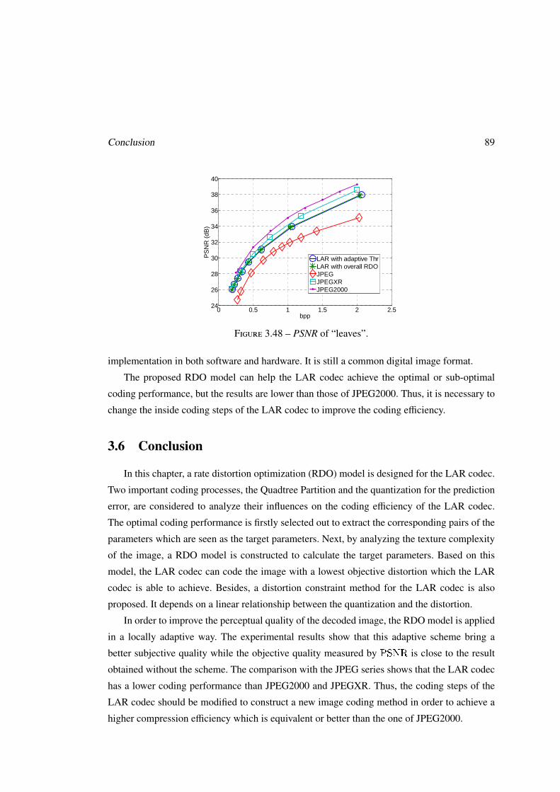
Conclusion 89
Louvre
leaves
0 0.5 1 1.5 2 2.520
25
30
35
40
45
bpp
PS
NR
(dB
)
LAR with adaptive ThrLAR with overall RDOJPEGJPEGXRJPEG2000
0 0.5 1 1.5 2 2.524
26
28
30
32
34
36
38
40
bpp
PS
NR
(dB
)
LAR with adaptive ThrLAR with overall RDOJPEGJPEGXRJPEG2000
Figure 3.48 – PSNR of “leaves”.
implementation in both software and hardware. It is still a common digital image format.
The proposed RDO model can help the LAR codec achieve the optimal or sub-optimal
coding performance, but the results are lower than those of JPEG2000. Thus, it is necessary to
change the inside coding steps of the LAR codec to improve the coding efficiency.
3.6 Conclusion
In this chapter, a rate distortion optimization (RDO) model is designed for the LAR codec.
Two important coding processes, the Quadtree Partition and the quantization for the prediction
error, are considered to analyze their influences on the coding efficiency of the LAR codec.
The optimal coding performance is firstly selected out to extract the corresponding pairs of the
parameters which are seen as the target parameters. Next, by analyzing the texture complexity
of the image, a RDO model is constructed to calculate the target parameters. Based on this
model, the LAR codec can code the image with a lowest objective distortion which the LAR
codec is able to achieve. Besides, a distortion constraint method for the LAR codec is also
proposed. It depends on a linear relationship between the quantization and the distortion.
In order to improve the perceptual quality of the decoded image, the RDO model is applied
in a locally adaptive way. The experimental results show that this adaptive scheme bring a
better subjective quality while the objective quality measured by PSNR is close to the result
obtained without the scheme. The comparison with the JPEG series shows that the LAR codec
has a lower coding performance than JPEG2000 and JPEGXR. Thus, the coding steps of the
LAR codec should be modified to construct a new image coding method in order to achieve a
higher compression efficiency which is equivalent or better than the one of JPEG2000.

90 Rate-distortion-optimization (RDO) model for LAR codec
Chapter 4
A low complexity lossless image codec :LAR-LLC
Due to the fast development of multimedia industry, the increasing demand of the media
data encourages the studies on promising technologies in order to efficiently make use of the
limited storage and communication capacity. Image compression plays an important role in this
field. In this chapter, the statement focuses on the scalable lossless image compression with
low complexity. Despite the wide use of lossy coding, for some applications, such as technical
drawing, art archiving, medical imaging and film post-production, the lossless compression is
more suitable for these high fidelity scenes. Therefore, the image coding standards, such as the
JPEG, JPEGXR and JPEG2000 also provide the lossless mode.
The compression ratio is the main indicator for evaluating the image compression method,
since the compression essentially aims at reducing the image storage space and the transmis-
sion capacity. For practical applications, the complexity is also a considerable performance
factor. In multimedia entertainment, such as Internet and High-definition television (HDTV),
high resolution images are generally desired by users. However, large size images need much
computations at the end which aggravate the coding latency. As a result, an efficient scalable
coding method with less computation is required to reduce the time-delay and adjust the image
resolution according to the channel capacity and user requirements. When implementing com-
pression techniques used in embedded systems such as digital cameras, and smart phones,
the low complexity coding algorithm is also preferable in order to reduce the electrical power
consumption and the processing time. In this context, reduced coding solutions are required for
both encoding and decoding parts. The compression methods often rely on two main stages :
a first decorrelation step based on transform and/or prediction techniques, and a final Variable
91
92 LAR-LLC
Length Coding (VLC) stage. As the VLC part is always a reversible process, the lossless co-
ding feature is generally only dependent on the first stage. For transform-based approaches, it
implies to use only reversible transforms, or to encode the residual errors after the transform.
Besides the standards, new methods are also proposed for specific image coding applica-
tions. Matsuda et al. designed an image coding scheme including a variable block-size adaptive
inter-color prediction technique [MKMI07]. This scheme requires a high computational com-
plexity of encoding due to an iterative optimization procedure. Zhao et al. applied a structure
learning and prediction scheme to the lossless image coding [ZH10]. This method is efficient
to images with rich high-frequency components, but also demands much computational com-
plexity caused by the expensive structure prediction. Pan et al. developed a low-complexity
screen compression scheme for lossy coding [PSL+13]. This scheme performs well on screen
images of texts, but underperforms JPEG2000 for natural images. Park et al. presented a low
complexity lossless image compression scheme using the context modeling and got compres-
sion results close to that of JPEGLS [PKC+10].
In this chapter, a lossless image coding method is introduced. It has the compression ef-
ficiency equivalent to JPEG2000, but lower computational complexity. This method is based
on the LAR (Locally Adaptive Resolution) framework. The extensions to the LAR codec are
also presented in [DBM06] and [BDR05] to implement the functions of the multi-resolution
and the lossless coding. The two articles introduce different pyramidal representations of the
image with the dyadic decomposition scheme for the multi-resolution. In [BDR05], the pro-
posed transform/prediction scheme called “Interleaved S+P” is directly derived from the “S
transform and Prediction (S+P) method” introduced in [SP93]. This scheme has been adopted
as the implementation of the LAR codec introduced in the chapter 2. Another dyadic decom-
position which is proposed in [DBM06] is based on the 2 × 2 block Walsh-Hadamard, with
a specific reversible mode (R-WHT) in the lossless context. This transform provides better
decorrelation performances than the “Interleaved S+P”, but at the expense of complexity.
The previous LAR codec did not achieve the compression efficiency as excellent as the
JPEG2000, and also required a medium computation cost about the same with JPEG2000.
Therefore, it is reasonable to design different coding stages based on the previous works in
order to raise the compression ratio while keeping the time consumption lower than those
of the standards. In this chapter, the proposed LAR-LLC (Lossless Low Complexity) coding
method adopts a 2×2 block transform called “Hierarchical Diagonal S Transform” (HD-ST). It
combines the advantages of the R-WHT and “S+P” for high decorrelation and low complexity,
respectively. A new inter and intra-levels prediction scheme is also introduced, with a very
Framework of Coding Scheme 93
limited complexity. Both transform and prediction are performed on the integer calculation
only.
For the VLC stage, the context adaptive arithmetic coders are generally preferred as they
provide significant gain by catching a part of the residual redundancy between symbols. Howe-
ver, these methods are also time-consuming [Sai04], [SBRM11]. The static Huffman coding is
a ideal choice for the low computational solution. In order to compensate the inherent loss of
compression efficiency compared with the arithmetic coder, a context modeling/classification
step before the VLC coding is introduced. Context modeling is an open problem in the image
coding, which has been widely analyzed in [Wu97], [PKC+10]. To avoid the problem of context
dilution and to reduce the complexity, a simple while efficient method of classification is intro-
duced. Based on the probability of distribution of the data source, we use a fixed context model
to classify the error stream into four sub-classes. The classification criterion is directly deduced
from the prediction error values, so the proposed scheme does not add significant processing
time overhead. Experiments show that the proposed low complexity lossless codec achieves a
compression ratio equivalent to JPEG2000, whereas it has much less coding latency.
The chapter is organized as follows. In Section 4.1, the general procedure of the proposed
lossless image coding method is presented. Section 4.2 introduces HD-ST transform to build
a pyramid structure for the multi-resolution. Section 4.3 introduces the prediction process ap-
plied for the reconstruction of the coded image based on lower resolution levels. Section 4.4
discusses the classification method for entropy coding. Results of the lossless coding efficiency
and the analysis of the complexity are provided in Section 4.5. Finally, this paper is concluded
in Section 4.6.
4.1 Framework of Coding Scheme
The proposed coder offers a scalable multi-resolution lossless image coding implementa-
tion. Fig. 4.1 shows the coder structure. The color image is firstly converted from RGB space to
Y Db Dr space [PSB+09]. As given in the equation (4.1), the Y Db Dr color space is reversible
and has a low computation complexity as only shift and addition operations are required. Be-
cause the green light contributes the most to the intensity perceived by humans, the luminance
Y reserves the half amplitude of the green element G, and quartered of the red and blue. The
chrominance Db and Dr represent the difference to G from B and R respectively. After the color
transform, the luminance Y and chrominance Db, Dr components are coded in parallel chan-
nels. In the pyramid structure, a multi-resolution image representation is built. Starting from
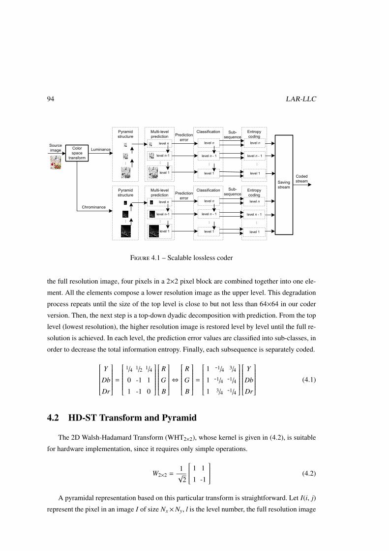
94 LAR-LLC
Color
space
transform
Source
image
Multi-level
prediction
level n
level n-1
...
level 1
Prediction
error
Pyramid
structure
Luminance
Chrominance
Multi-level
prediction
level n
level n-1
...level 1
Pyramid
structure
Classification
level n
level n - 1
level 1
...
Classification
level n
level n - 1
level 1
...
Prediction
error
......
Sub-
sequence
Entropy
coding
level n
level n - 1
level 1
...
Entropy
coding
level n
level n - 1
level 1
...
Saving
stream
Coded
stream
Sub-
sequence
Figure 4.1 – Scalable lossless coder
the full resolution image, four pixels in a 2×2 pixel block are combined together into one ele-
ment. All the elements compose a lower resolution image as the upper level. This degradation
process repeats until the size of the top level is close to but not less than 64×64 in our coder
version. Then, the next step is a top-down dyadic decomposition with prediction. From the top
level (lowest resolution), the higher resolution image is restored level by level until the full re-
solution is achieved. In each level, the prediction error values are classified into sub-classes, in
order to decrease the total information entropy. Finally, each subsequence is separately coded.Y
Db
Dr
=
1/4 1/2 1/4
0 -1 1
1 -1 0
R
G
B
⇔
R
G
B
=
1 -1/4 3/4
1 -1/4 -1/4
1 3/4 -1/4
Y
Db
Dr
(4.1)
4.2 HD-ST Transform and Pyramid
The 2D Walsh-Hadamard Transform (WHT2×2), whose kernel is given in (4.2), is suitable
for hardware implementation, since it requires only simple operations.
W2×2 =1√
2
1 1
1 -1
(4.2)
A pyramidal representation based on this particular transform is straightforward. Let I(i, j)
represent the pixel in an image I of size Nx ×Ny, l is the level number, the full resolution image
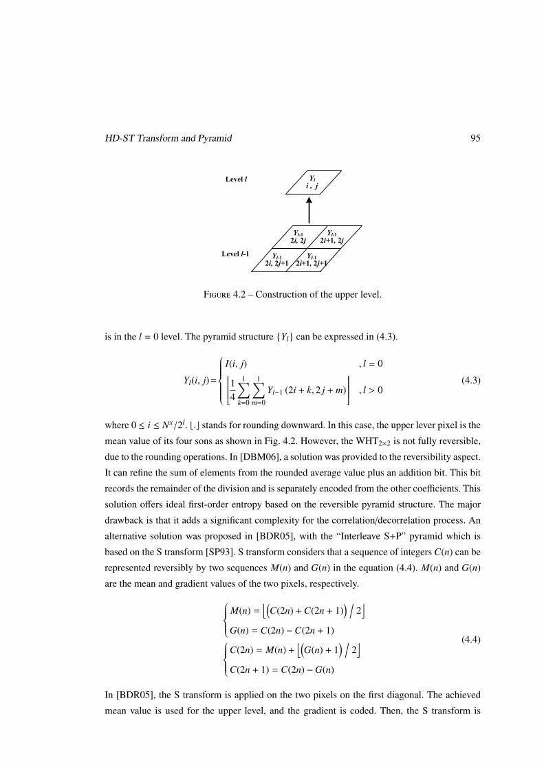
HD-ST Transform and Pyramid 95
Yl-1
2i, 2jYl-1
2i+1, 2j
Yl-1
2i, 2j+1
Yl-1
2i+1, 2j+1
Yl
i , j
Level l-1
Level l
Figure 4.2 – Construction of the upper level.
is in the l = 0 level. The pyramid structure {Yl} can be expressed in (4.3).
Yl(i, j)=
I(i, j) , l = 014
1∑k=0
1∑m=0
Yl−1 (2i + k, 2 j + m)
, l > 0(4.3)
where 0 ≤ i ≤ Nx/2l. b.c stands for rounding downward. In this case, the upper lever pixel is the
mean value of its four sons as shown in Fig. 4.2. However, the WHT2×2 is not fully reversible,
due to the rounding operations. In [DBM06], a solution was provided to the reversibility aspect.
It can refine the sum of elements from the rounded average value plus an addition bit. This bit
records the remainder of the division and is separately encoded from the other coefficients. This
solution offers ideal first-order entropy based on the reversible pyramid structure. The major
drawback is that it adds a significant complexity for the correlation/decorrelation process. An
alternative solution was proposed in [BDR05], with the “Interleave S+P” pyramid which is
based on the S transform [SP93]. S transform considers that a sequence of integers C(n) can be
represented reversibly by two sequences M(n) and G(n) in the equation (4.4). M(n) and G(n)
are the mean and gradient values of the two pixels, respectively. M(n) =⌊(
C(2n) + C(2n + 1)) /
2⌋
G(n) = C(2n) −C(2n + 1)C(2n) = M(n) +⌊(
G(n) + 1) /
2⌋
C(2n + 1) = C(2n) −G(n)
(4.4)
In [BDR05], the S transform is applied on the two pixels on the first diagonal. The achieved
mean value is used for the upper level, and the gradient is coded. Then, the S transform is
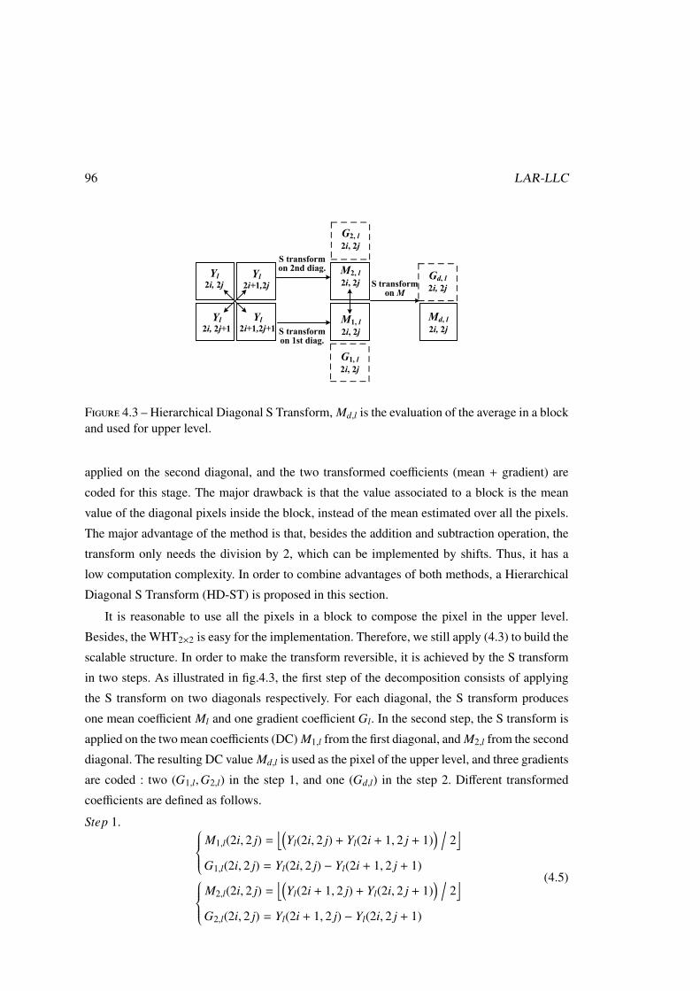
96 LAR-LLC
Yl
2i, 2j
Yl
2i+1,2j+1
Yl
2i, 2j+1
Yl
2i+1,2j
S transform on 1st diag.
S transform on 2nd diag.
M1, l
2i, 2j
G1, l
2i, 2j
M2, l
2i, 2j
G2, l
2i, 2j
S transform on M
Md, l
2i, 2j
Gd, l
2i, 2j
Yl
2i, 2j
Yl
2i+2,2j+2
Yl
2i+1,2j+1
Yl
2i-1, 2j
Yl
2i-1, 2j-1
Yl
2i+1, 2j-1
Xl
2i+1,2j+2
Xl
2i+2,2j+1
Yl
2i-1,2j+1
Yl
2i, 2j-1
Yl
2i+2, 2j-1
Yl
2i,2j+2
Yl
2i+2, 2j
Xl
2i-1, 2j+2
Xl2i+1, 2j
Xl2i, 2j+1
el
2i-2, 2j-2
Level l
Level l + 1
el
2i, 2j-2
el
2i-2, 2j
el
2i+2, 2j-2
el + 1
i, j
el
2i, 2j
Xl
2i+2,2j+2
Xl
2i-1, 2j
Yl
2i-1, 2j-1
Yl
2i-2, 2j-2
Yl
2i, 2j-2
Yl
2i+1, 2j-1
Xl
2i+1,2j+2
Xl
2i+2,2j+1
Yl
2i-2, 2j
Yl
2i-1,2j+1
Xl
2i, 2j-1
Yl
2i+2,2j-2
Xl
Xl
2i, 2j
Xl
2i+1, 2j+1
Xl2i+1, 2j
Xl
2i, 2j+1
(a) Positions of referred pixels (b) Evaluation of X
Figure 4.3 – Hierarchical Diagonal S Transform, Md,l is the evaluation of the average in a blockand used for upper level.
applied on the second diagonal, and the two transformed coefficients (mean + gradient) are
coded for this stage. The major drawback is that the value associated to a block is the mean
value of the diagonal pixels inside the block, instead of the mean estimated over all the pixels.
The major advantage of the method is that, besides the addition and subtraction operation, the
transform only needs the division by 2, which can be implemented by shifts. Thus, it has a
low computation complexity. In order to combine advantages of both methods, a Hierarchical
Diagonal S Transform (HD-ST) is proposed in this section.
It is reasonable to use all the pixels in a block to compose the pixel in the upper level.
Besides, the WHT2×2 is easy for the implementation. Therefore, we still apply (4.3) to build the
scalable structure. In order to make the transform reversible, it is achieved by the S transform
in two steps. As illustrated in fig.4.3, the first step of the decomposition consists of applying
the S transform on two diagonals respectively. For each diagonal, the S transform produces
one mean coefficient Ml and one gradient coefficient Gl. In the second step, the S transform is
applied on the two mean coefficients (DC) M1,l from the first diagonal, and M2,l from the second
diagonal. The resulting DC value Md,l is used as the pixel of the upper level, and three gradients
are coded : two (G1,l,G2,l) in the step 1, and one (Gd,l) in the step 2. Different transformed
coefficients are defined as follows.
Step 1. M1,l(2i, 2 j) =⌊(
Yl(2i, 2 j) + Yl(2i + 1, 2 j + 1)) /
2⌋
G1,l(2i, 2 j) = Yl(2i, 2 j) − Yl(2i + 1, 2 j + 1) M2,l(2i, 2 j) =⌊(
Yl(2i + 1, 2 j) + Yl(2i, 2 j + 1)) /
2⌋
G2,l(2i, 2 j) = Yl(2i + 1, 2 j) − Yl(2i, 2 j + 1)
(4.5)
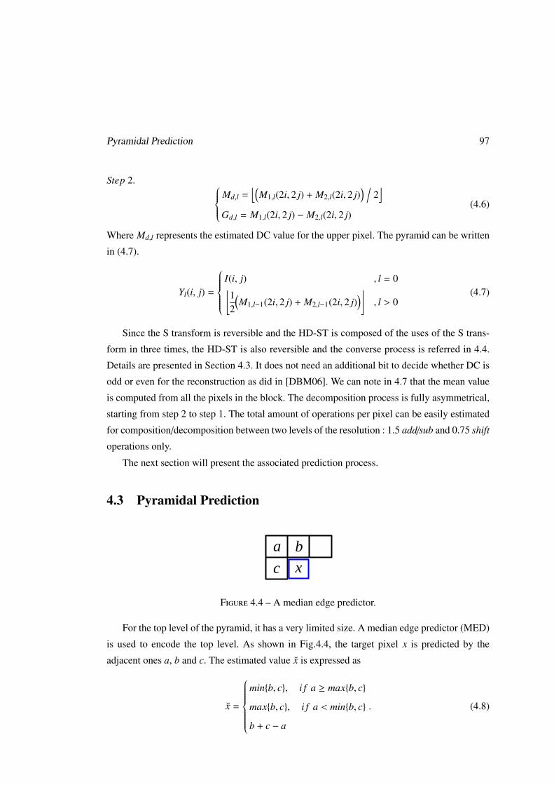
Pyramidal Prediction 97
Step 2. Md,l =⌊(
M1,l(2i, 2 j) + M2,l(2i, 2 j)) /
2⌋
Gd,l = M1,l(2i, 2 j) − M2,l(2i, 2 j)(4.6)
Where Md,l represents the estimated DC value for the upper pixel. The pyramid can be written
in (4.7).
Yl(i, j) =
I(i, j) , l = 0⌊
12
(M1,l−1(2i, 2 j) + M2,l−1(2i, 2 j)
)⌋, l > 0
(4.7)
Since the S transform is reversible and the HD-ST is composed of the uses of the S trans-
form in three times, the HD-ST is also reversible and the converse process is referred in 4.4.
Details are presented in Section 4.3. It does not need an additional bit to decide whether DC is
odd or even for the reconstruction as did in [DBM06]. We can note in 4.7 that the mean value
is computed from all the pixels in the block. The decomposition process is fully asymmetrical,
starting from step 2 to step 1. The total amount of operations per pixel can be easily estimated
for composition/decomposition between two levels of the resolution : 1.5 add/sub and 0.75 shift
operations only.
The next section will present the associated prediction process.
4.3 Pyramidal Prediction
x
a b
c
Figure 4.4 – A median edge predictor.
For the top level of the pyramid, it has a very limited size. A median edge predictor (MED)
is used to encode the top level. As shown in Fig.4.4, the target pixel x is predicted by the
adjacent ones a, b and c. The estimated value x is expressed as
x =
min{b, c}, i f a ≥ max{b, c}
max{b, c}, i f a < min{b, c}
b + c − a
. (4.8)
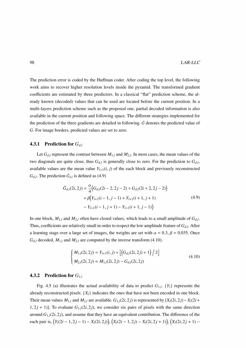
98 LAR-LLC
The prediction error is coded by the Huffman coder. After coding the top level, the following
work aims to recover higher resolution levels inside the pyramid. The transformed gradient
coefficients are estimated by three predictors. In a classical “flat” prediction scheme, the al-
ready known (decoded) values that can be used are located before the current position. In a
multi-layers prediction scheme such as the proposed one, partial decoded information is also
available in the current position and following space. The different strategies implemented for
the prediction of the three gradients are detailed in following. G denotes the predicted value of
G. For image borders, predicted values are set to zero.
4.3.1 Prediction for Gd,l
Let Gd,l represent the contrast between M1,l and M2,l. In most cases, the mean values of the
two diagonals are quite close, thus Gd,l is generally close to zero. For the prediction to Gd,l,
available values are the mean value Yl+1(i, j) of the each block and previously reconstructed
Gd,l. The prediction Gd,l is defined as (4.9)
Gd,l(2i, 2 j) =α
4
(Gd,l(2i − 2, 2 j − 2) + Gd,l(2i + 2, 2 j − 2)
)+ β
(Yl+1(i − 1, j − 1) + Yl+1(i + 1, j + 1)
− Yl+1(i − 1, j + 1) − Yl+1(i + 1, j − 1)) (4.9)
In one block, M1,l and M2,l often have closed values, which leads to a small amplitude of Gd,l.
Thus, coefficients are relatively small in order to respect the low amplitude feature of Gd,l. After
a learning stage over a large set of images, the weights are set with α = 0.3, β = 0.035. Once
Gd,l decoded, M1,l and M2,l are computed by the inverse transform (4.10). M1,l(2i, 2 j) = Yl+1(i, j) +⌊(
Gd,l(2i, 2 j) + 1) /
2⌋
M2,l(2i, 2 j) = M1,l(2i, 2 j) −Gd,l(2i, 2 j)(4.10)
4.3.2 Prediction for G1,l
Fig. 4.5 (a) illustrates the actual availability of data to predict G1,l. {Yl} represents the
already reconstructed pixels. {Xl} indicates the ones that have not been encoded in one block.
Their mean values M1,l and M2,l are available. G1,l(2i, 2 j) is represented by [Xl(2i, 2 j)−Xl(2i +
1, 2 j + 1)]. To evaluate G1,l(2i, 2 j), we consider six pairs of pixels with the same direction
around G1,l(2i, 2 j), and assume that they have an equivalent contribution. The difference of the
each pair is,(Yl(2i − 1, 2 j − 1) − Xl(2i, 2 j)
),(Xl(2i − 1, 2 j) − Xl(2i, 2 j + 1)
),(Xl(2i, 2 j + 1) −
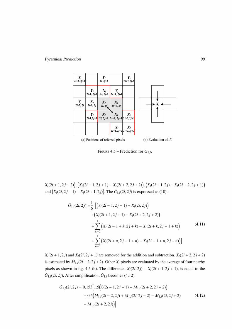
Pyramidal Prediction 99
Yl
2i, 2j
Yl
2i+1,2j+1
Yl
2i, 2j+1
Yl
2i+1,2j
S transform on 1st diag.
S transform on 2nd diag.
M1, l
2i, 2j
G1, l
2i, 2j
M2, l
2i, 2j
G2, l
2i, 2j
S transform on M
Md, l
2i, 2j
Gd, l
2i, 2j
Yl
2i, 2j
Yl
2i+2,2j+2
Yl
2i+1,2j+1
Yl
2i-1, 2j
Yl
2i-1, 2j-1
Yl
2i+1, 2j-1
Xl
2i+1,2j+2
Xl
2i+2,2j+1
Yl
2i-1,2j+1
Yl
2i, 2j-1
Yl
2i+2, 2j-1
Yl
2i,2j+2
Yl
2i+2, 2j
Xl
2i-1, 2j+2
Xl2i+1, 2j
Xl2i, 2j+1
el2i-2, 2j-2
Level l
Level l + 1
el2i, 2j-2
el2i-2, 2j
el2i+2, 2j-2
el + 1i, j
el2i, 2j
Xl
2i+2,2j+2
Xl
2i-1, 2j
Yl
2i-1, 2j-1
Yl
2i-2, 2j-2
Yl
2i, 2j-2
Yl
2i+1, 2j-1
Xl
2i+1,2j+2
Xl
2i+2,2j+1
Yl
2i-2, 2j
Yl
2i-1,2j+1
Xl
2i, 2j-1
Yl
2i+2,2j-2
XlXl
2i, 2j
Xl
2i+1, 2j+1
Xl2i+1, 2j
Xl
2i, 2j+1
(a) Positions of referred pixels
(b) Evaluation of X
Xl2i+2,2j+2
Xl2i-1, 2j
Yl2i-1, 2j-1
Yl2i-2, 2j-2
Yl2i, 2j-2
Yl2i+1, 2j-1
Xl2i+1,2j+2
Xl
2i+2,2j+1
Yl2i-2, 2j
Yl
2i-1,2j+1
Xl2i, 2j-1
Yl2i+2,2j-2
XlXl
2i, 2j
Xl
2i+1, 2j+1
Xl2i+1, 2j
Xl
2i, 2j+1
(a) Positions of referred pixels (b) Evaluation of X
Yl2i, 2j
Yl2i+2,2j+2
Yl2i+1,2j+1
Yl2i-1, 2j
Yl2i-1, 2j-1
Yl2i+1, 2j-1
Xl2i+1,2j+2
Xl2i+2,2j+1
Yl2i-1,2j+1
Yl2i, 2j-1
Yl2i+2, 2j-1
Yl2i,2j+2
Yl2i+2, 2j
Xl2i-1, 2j+2
Xl2i+1, 2j
Xl2i, 2j+1
Figure 4.5 – Prediction for G1,l.
Xl(2i + 1, 2 j + 2)),(Xl(2i − 1, 2 j + 1) − Xl(2i + 2, 2 j + 2)
),(Xl(2i + 1, 2 j) − Xl(2i + 2, 2 j + 1)
)and
(Xl(2i, 2 j − 1) − Xl(2i + 1, 2 j)
). The G1,l(2i, 2 j) is expressed as (10).
G1,l(2i, 2 j) =16
[(Yl(2i − 1, 2 j − 1) − Xl(2i, 2 j)
)+(Xl(2i + 1, 2 j + 1) − Xl(2i + 2, 2 j + 2)
)+
1∑k=0
(Xl(2i − 1 + k, 2 j + k) − Xl(2i + k, 2 j + 1 + k)
)+
1∑n=0
(Xl(2i + n, 2 j − 1 + n) − Xl(2i + 1 + n, 2 j + n)
)](4.11)
Xl(2i + 1, 2 j) and Xl(2i, 2 j + 1) are removed for the addition and subtraction. Xl(2i + 2, 2 j + 2)
is estimated by M1,l(2i + 2, 2 j + 2). Other Xl pixels are evaluated by the average of four nearby
pixels as shown in fig. 4.5 (b). The difference, Xl(2i, 2 j) − Xl(2i + 1, 2 j + 1), is equal to the
G1,l(2i, 2 j). After simplification, G1,l becomes (4.12).
G1,l(2i, 2 j) = 0.153[1.5
(Yl(2i − 1, 2 j − 1) − M1,l(2i + 2, 2 j + 2)
)+ 0.5
(M1,l(2i − 2, 2 j) + M1,l(2i, 2 j − 2) − M1,l(2i, 2 j + 2)
− M1,l(2i + 2, 2 j))] (4.12)
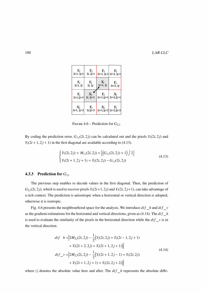
100 LAR-LLC
Yl
2i, 2j
Yl
2i+1,2j+1
Yl
2i, 2j+1
Yl
2i+1,2j
S transform on 1st diag.
S transform on 2nd diag.
M1, l
2i, 2j
G1, l
2i, 2j
M2, l
2i, 2j
G2, l
2i, 2j
S transform on M
Md, l
2i, 2j
Gd, l
2i, 2j
Yl
2i, 2j
Yl
2i+2,2j+2
Yl
2i+1,2j+1
Yl
2i-1, 2j
Yl
2i-1, 2j-1
Yl
2i+1, 2j-1
Xl
2i+1,2j+2
Xl
2i+2,2j+1
Yl
2i-1,2j+1
Yl
2i, 2j-1
Yl
2i+2, 2j-1
Yl
2i,2j+2
Yl
2i+2, 2j
Xl
2i-1, 2j+2
Xl2i+1, 2j
Xl2i, 2j+1
el
2i-2, 2j-2
Level l
Level l + 1
el
2i, 2j-2
el
2i-2, 2j
el
2i+2, 2j-2
el + 1
i, j
el
2i, 2j
Xl
2i+2,2j+2
Xl
2i-1, 2j
Yl
2i-1, 2j-1
Yl
2i-2, 2j-2
Yl
2i, 2j-2
Yl
2i+1, 2j-1
Xl
2i+1,2j+2
Xl
2i+2,2j+1
Yl
2i-2, 2j
Yl
2i-1,2j+1
Xl
2i, 2j-1
Yl
2i+2,2j-2
XlXl
2i, 2j
Xl
2i+1, 2j+1
Xl2i+1, 2j
Xl
2i, 2j+1
(a) Positions of referred pixels
(b) Evaluation of X
Xl2i+2,2j+2
Xl2i-1, 2j
Yl2i-1, 2j-1
Yl2i-2, 2j-2
Yl2i, 2j-2
Yl2i+1, 2j-1
Xl2i+1,2j+2
Xl
2i+2,2j+1
Yl2i-2, 2j
Yl
2i-1,2j+1
Xl2i, 2j-1
Yl2i+2,2j-2
XlXl
2i, 2j
Xl
2i+1, 2j+1
Xl2i+1, 2j
Xl
2i, 2j+1
(a) Positions of referred pixels (b) Evaluation of X
Yl2i, 2j
Yl2i+2,2j+2
Yl2i+1,2j+1
Yl2i-1, 2j
Yl2i-1, 2j-1
Yl2i+1, 2j-1
Xl2i+1,2j+2
Xl2i+2,2j+1
Yl2i-1,2j+1
Yl2i, 2j-1
Yl2i+2, 2j-1
Yl2i,2j+2
Yl2i+2, 2j
Xl2i-1, 2j+2
Xl2i+1, 2j
Xl2i, 2j+1
Figure 4.6 – Prediction for G2,l.
By coding the prediction error, G1,l(2i, 2 j) can be calculated out and the pixels Yl(2i, 2 j) and
Yl(2i + 1, 2 j + 1) in the first diagonal are available according to (4.13). Yl(2i, 2 j) = M1,l(2i, 2 j) +⌊(
G1,l(2i, 2 j) + 1) /
2⌋
Yl(2i + 1, 2 j + 1) = Yl(2i, 2 j) −G1,l(2i, 2 j)(4.13)
4.3.3 Prediction for G2,l
The previous step enables to decode values in the first diagonal. Then, the prediction of
G2,l(2i, 2 j), which is used to recover pixels Yl(2i+1, 2 j) and Yl(2i, 2 j+1), can take advantage of
a rich context. The prediction is anisotropic when a horizontal or vertical direction is adopted,
otherwise it is isotropic.
Fig. 4.6 presents the neighbourhood space for the analysis. We introduce di f_h and di f_v
as the gradient estimations for the horizontal and vertical directions, given as (4.14). The di f_h
is used to evaluate the similarity of the pixels in the horizontal direction while the di f_v is in
the vertical direction.
di f_h =∣∣∣∣2M2,l(2i, 2 j) −
12
(Yl(2i, 2 j) + Yl(2i − 1, 2 j + 1)
+ Yl(2i + 2, 2 j) + Yl(2i + 1, 2 j + 1))∣∣∣∣
di f_v =∣∣∣∣2M2,l(2i, 2 j) −
12
(Yl(2i + 1, 2 j − 1) + Yl(2i, 2 j)
+ Yl(2i + 1, 2 j + 1) + Yl(2i, 2 j + 2))∣∣∣∣
(4.14)
where |.| denotes the absolute value here and after. The di f_h represents the absolute diffe-
Pyramidal Prediction 101
rence between the second mean value M2,l(2i, 2 j) and the average of the adjacent pixels in the
horizontal direction, and the di f_v represents the one in the vertical direction. A large value
of di f_h or di f_v is often due to the presence of an edge. In that case, a better estimation can
be achieved by a directional prediction. Therefore, the prediction of G2,l(2i, 2 j) is treated for
the “flat” part and “edge” part respectively. In this implementation, we set a threshold to 20 to
separate the prediction into two branches. We set this threshold value in order to keep a weight
coefficient α no less than 95.5% when di f_h = 1 for the “edge” prediction in the Branch 1. α
is given by
α =di f_v
di f_h + di f_v. (4.15)
Similarly, (1 − α) is not less than 95.5% when di f_v = 1.
Branch 1 : If one of di f_h and di f_v, or both are greater than the threshold, this block
is considered in an “edge” part. The proposed predictor is defined as (4.16). When di f_h is
greater than di f_v, it probably means the “edge” is in vertical direction. Thus, the contribution
from the vertical direction is favored 1 − α is greater than α.
G2,l(2i, 2 j) =α
2
(Yl(2i, 2 j) − Yl(2i − 1, 2 j + 1) + Yl(2i + 2, 2 j) − Yl(2i + 1, 2 j + 1)
)+
1 − α2
(Yl(2i + 1, 2 j − 1) − Yl(2i, 2 j) + Yl(2i + 1, 2 j + 1)
− Yl(2i, 2 j + 2)) (4.16)
Branch 2 : If both di f_h and di f_v are not greater than the threshold, a smoother predic-
tion is suited to G2,l(2i, 2 j), given in (4.17).
G2,l(2i, 2 j) =38
(Yl(2i + 1, 2 j − 1) + Yl(2i + 2, 2 j) − Yl(2i − 1, 2 j + 1) − Yl(2i, 2 j + 2)
)−
18
(Yl(2i, 2 j − 1) + Yl(2i + 2, 2 j − 1) − Yl(2i − 1, 2 j) − Xl(2i + 1, 2 j)
) (4.17)
Xl(2i + 1, 2 j) is estimated by Wu’s predictor for the third pass [Wu97].
Xl(2i + 1, 2 j) =38
(Yl(2i, 2 j) + Yl(2i + 1, 2 j − 1) + Yl(2i + 2, 2 j) + Yl(2i + 1, 2 j + 1)
)−
14
(Yl(2i, 2 j − 1) + Yl(2i + 2, 2 j − 1)
) (4.18)
The floating-point operations are much more complex and time-consuming than the integer
ones for both software and hardware implementations [CLHH09]. Thus, we approximate the
floating-point multiplication by simple integer operations, such as the add/sub and shift. The
102 LAR-LLC
division by 2m (m ≥ 0, m is an integer) can be achieved by right-shift in m times, denoted by
(>> m), while the multiplication with 2n (n ≥ 0, n is an integer) can be achieved by left-shift
in n times, denoted by (<< n). For the prediction of the Gd,l, the coefficient 0.3 is approxima-
ted by ( 14 + 1
8 −116 = 0.3125), 0.035 is ( 1
32 + 1256 = 0.03515). For G1,l, the coefficient 0.153
is approximated by ( 18 + 1
32 −1
256 = 0.1523). The multiplications with these coefficients are
estimated by (4.19),
0.3 · X ≈ (X >> 2) + (X >> 3) − (X >> 4)
0.035 · X ≈ (X >> 5) + (X >> 8)
0.153 · X ≈ (X >> 3) + (X >> 5) − (X >> 8)
(4.19)
where X represents the multiplier. The division operation is only required for G2,l in (4.16).
After this step, pixels in the second diagonal are available in (4.20). Yl(2i + 1, 2 j) = M2,l(2i, 2 j) +⌊(
G2,l(2i, 2 j) + 1) /
2⌋
Yl(2i, 2 j + 1) = Yl(2i + 1, 2 j) −G2,l(2i, 2 j)(4.20)
4.4 Entropy Pre-coding and Coding of Prediction Errors
Context adaptive arithmetic coders are efficient solutions for VLC encoding. However,
the complexity is still considered to be higher than the Huffman one [Sai04]. For the “ultra-
fast” mode of JPEG2000, T. Ritcher et al. replaced the EBCOT coding by a simple Huffman-
runlength one [RS12]. Similarly, a Pre-coding+Huffman scheme is adopted in this section.
For the Huffman coding, we adopt the classic static mode rather than the adaptive mode.
The former generates a non-adaptive codebook from the data source, and then codes symbols
by pre-fixed codebook elements. The latter often uses the feedback loop and delays the coding
because of the limitation on the amount of symbols to be each time handled. Before the Huff-
man coder, a pre-coding step consisting in a pre-classifying symbols is applied to increase the
coding gain. This concept is based on the source separation theory : the global entropy of a
source can be reduced if the source is “well” separated into sub-sources with different Probabi-
lity Distributions (PD) [HDG92]. The implementation of pre-coding is dependent on the ove-
rall coding scheme. Marpe et al. [MC97] propose a partitioning, aggregation and conditional
coding (PACC) based on the discrete wavelet transform. Further, they use an adaptive binary
arithmetic coding to reduce the alphabet size of quantized transform coefficients [MSW03].
Instead of the arithmetic coding, LAR-LLC adopts the Huffman coding and focuses on the
Entropy Pre-coding and Coding of Prediction Errors 103
arrangement of PD. The details are introduced here.
After prediction, most residual errors have small amplitudes, and the distribution function
is symmetric around zero. A suitable classification solution would be to separate errors ac-
cording to their amplitude. The following part gives an analysis on the change of the source
entropy by the use of the amplitude classification. The error stream can be considered as a finite
input sequence A of a discrete memoryless source with a alphabet set U = {a1, a2, ..., an}. The
sequence A has a length N. Ni is the amount of the symbol ai (1 ≤ i ≤ n) in this sequence. Let
the probability of a symbol ai be
pA(ai) =Ni
N, 1 ≤ i ≤ n. (4.21)
The entropy of the sequence can be expressed by Eq. (4.22). H(A) gives the lower bound of the
average code length L for each symbol to losslessly encode A.
H(A) = −
n∑i=1
pA(ai) · log2 pA(ai) (4.22)
The least totally required code length is NH(A). Consider any subsequence A1 with a length
N1 and A2 with a length N2, A1 ∈ U1 = {a1, a2, ..., an1} and A2 ∈ U2 = {an1+1, an1+2, ..., an}.
Then U = U1 ∪ U2 and U1 ∩ U2 = ∅. It has N = N1 + N2, and the least required code length
can be expressed by (4.23) when coding A1 and A2 separately.
N1H(A1) + N2H(A2) = −N1
n1∑j=1
pA1(a j) · log2 pA1(a j)− N2
n∑k=n1+1
pA2(ak) · log2 pA2(ak) (4.23)
where pA1(a j) is the probability of a j in subsequence A1 and pA2(ak) is the probability of ak in
A2. Notice that N1 pA1(a j) equals to N p(a j), and N2 pA2(ak) equals to N p(ak). Let α = (N1/N)
(0 < α < 1), then (4.23) can be simplified as
N1H(A1) + N2H(A2) =N
− n1∑j=1
pA(a j) · log2 pA(a j) −n∑
k=n1+1
pA(ak) · log2 pA(ak)
+ N
n1∑j=1
pA1(a j) · log2N1
N+
n∑k=n1+1
pA2(ak) · log2N2
N
=NH(A) + N
[α · log2α + (1 − α) · log2(1 − α)
](4.24)
Let [ −α · log2α − (1 − α) · log2(1 − α)] be β, it can be achieved that
104 LAR-LLC
N1H(A1) + N2H(A2) = N[H(A) − β
]≤ N H(A)
(4.25)
where 0 ≤ β ≤ 1.
The length 4.25 has the minimum value N(H(A) − 1) when α = 0.5. It is noticed that the
required code length descends after the classification, and at most 1 bit is saved while N1 equals
to N2. The saved 1 bit indicates the reduction of the range of the sub alphabet of A1 and A2
compared to the alphabet of A. In order to reduce the alphabet set by the classification, one
possible way is to separate errors according to their amplitude and separately encode them.
This classification allocates the elements of the error sequence into sub-sequences. The sub-
sequences should have the equal length.
The side information will be needed for the decoder in order to recover the sub-sequences
exactly during the decoding process. For instance, in this binary classification, 1 bit is required
to indicate which class has been chosen for the current prediction error. The side information
increases the bitrate and overbalances the potential benefit of the entropy reduction. To avoid
this side information, we prefer a prior classification, and the pre-coding in LAR-LLC mainly
consists of defining good error amplitude estimation based on the information around the cur-
rent position.
In order to find an efficient, but not computationally complex estimation method, we have
investigated different criteria such as the amplitude of the gradient prediction, co-located errors
for previous gradient, and errors of the upper level. Eventually, the available prediction errors
from adjacent positions at current level and the corresponding one at upper level are considered
together for a notable improvement in the coding efficiency. The classification method based
on it is introduced in the following.
Let el(2i, 2 j) be the current prediction error of any G component in a block. The evaluated
value of its amplitude el_apt(2i, 2 j) is defined as (4.26).Coeadjacent =
14
(∣∣∣∣el(2i − 2, 2 j)∣∣∣∣+∣∣∣∣el(2i, 2 j − 2)
∣∣∣∣+∣∣∣∣el(2i − 2, 2 j − 2)
∣∣∣∣ +∣∣∣∣el(2i + 2, 2 j − 2)
∣∣∣∣)Coeupper =
∣∣∣∣el+1(i, j)∣∣∣∣
⇒ el_apt(2i, 2 j) =34
Coead jacent +14
Coeupper
(4.26)
In (4.26), Coead jacent is the average of adjacent available errors, Coeupper is the one from upper
level. Their positions are shown in Fig. 4.7 .
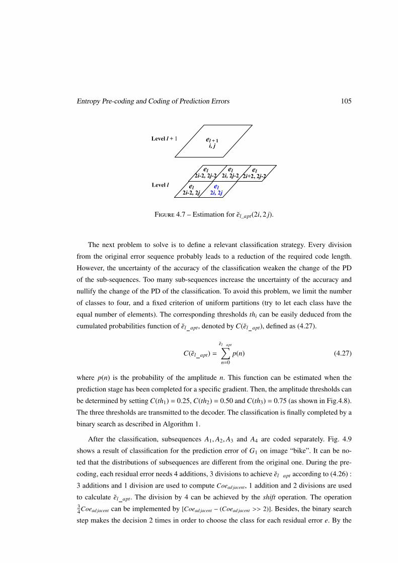
Entropy Pre-coding and Coding of Prediction Errors 105
Yl
2i, 2j
Yl
2i+1,2j+1
Yl
2i, 2j+1
Yl
2i+1,2j
S transform on 1st diag.
S transform on 2nd diag.
M1, l
2i, 2j
G1, l
2i, 2j
M2, l
2i, 2j
G2, l
2i, 2j
S transform on M
Md, l
2i, 2j
Gd, l
2i, 2j
Yl
2i, 2j
Yl
2i+2,2j+2
Yl
2i+1,2j+1
Yl
2i-1, 2j
Yl
2i-1, 2j-1
Yl
2i+1, 2j-1
Xl
2i+1,2j+2
Xl
2i+2,2j+1
Yl
2i-1,2j+1
Yl
2i, 2j-1
Yl
2i+2, 2j-1
Yl
2i,2j+2
Yl
2i+2, 2j
Xl
2i-1, 2j+2
Xl2i+1, 2j
Xl2i, 2j+1
el2i-2, 2j-2
Level l
Level l + 1
el2i, 2j-2
el2i-2, 2j
el2i+2, 2j-2
el + 1i, j
el2i, 2j
Xl
2i+2,2j+2
Xl
2i-1, 2j
Yl
2i-1, 2j-1
Yl
2i-2, 2j-2
Yl
2i, 2j-2
Yl
2i+1, 2j-1
Xl
2i+1,2j+2
Xl
2i+2,2j+1
Yl
2i-2, 2j
Yl
2i-1,2j+1
Xl
2i, 2j-1
Yl
2i+2,2j-2
XlXl
2i, 2j
Xl
2i+1, 2j+1
Xl2i+1, 2j
Xl
2i, 2j+1
(a) Positions of referred pixels
(b) Evaluation of X
Xl2i+2,2j+2
Xl2i-1, 2j
Yl2i-1, 2j-1
Yl2i-2, 2j-2
Yl2i, 2j-2
Yl2i+1, 2j-1
Xl2i+1,2j+2
Xl
2i+2,2j+1
Yl2i-2, 2j
Yl
2i-1,2j+1
Xl2i, 2j-1
Yl2i+2,2j-2
XlXl
2i, 2j
Xl
2i+1, 2j+1
Xl2i+1, 2j
Xl
2i, 2j+1
(a) Positions of referred pixels (b) Evaluation of X
Yl2i, 2j
Yl2i+2,2j+2
Yl2i+1,2j+1
Yl2i-1, 2j
Yl2i-1, 2j-1
Yl2i+1, 2j-1
Xl2i+1,2j+2
Xl2i+2,2j+1
Yl2i-1,2j+1
Yl2i, 2j-1
Yl2i+2, 2j-1
Yl2i,2j+2
Yl2i+2, 2j
Xl2i-1, 2j+2
Xl2i+1, 2j
Xl2i, 2j+1
Figure 4.7 – Estimation for el_apt(2i, 2 j).
The next problem to solve is to define a relevant classification strategy. Every division
from the original error sequence probably leads to a reduction of the required code length.
However, the uncertainty of the accuracy of the classification weaken the change of the PD
of the sub-sequences. Too many sub-sequences increase the uncertainty of the accuracy and
nullify the change of the PD of the classification. To avoid this problem, we limit the number
of classes to four, and a fixed criterion of uniform partitions (try to let each class have the
equal number of elements). The corresponding thresholds thi can be easily deduced from the
cumulated probabilities function of el_apt, denoted by C(el_apt), defined as (4.27).
C(el_apt) =
el_apt∑n=0
p(n) (4.27)
where p(n) is the probability of the amplitude n. This function can be estimated when the
prediction stage has been completed for a specific gradient. Then, the amplitude thresholds can
be determined by setting C(th1) = 0.25, C(th2) = 0.50 and C(th3) = 0.75 (as shown in Fig.4.8).
The three thresholds are transmitted to the decoder. The classification is finally completed by a
binary search as described in Algorithm 1.
After the classification, subsequences A1, A2, A3 and A4 are coded separately. Fig. 4.9
shows a result of classification for the prediction error of G1 on image “bike”. It can be no-
ted that the distributions of subsequences are different from the original one. During the pre-
coding, each residual error needs 4 additions, 3 divisions to achieve el_apt according to (4.26) :
3 additions and 1 division are used to compute Coead jacent, 1 addition and 2 divisions are used
to calculate el_apt. The division by 4 can be achieved by the shift operation. The operation34Coead jacent can be implemented by [Coead jacent − (Coead jacent >> 2)]. Besides, the binary search
step makes the decision 2 times in order to choose the class for each residual error e. By the
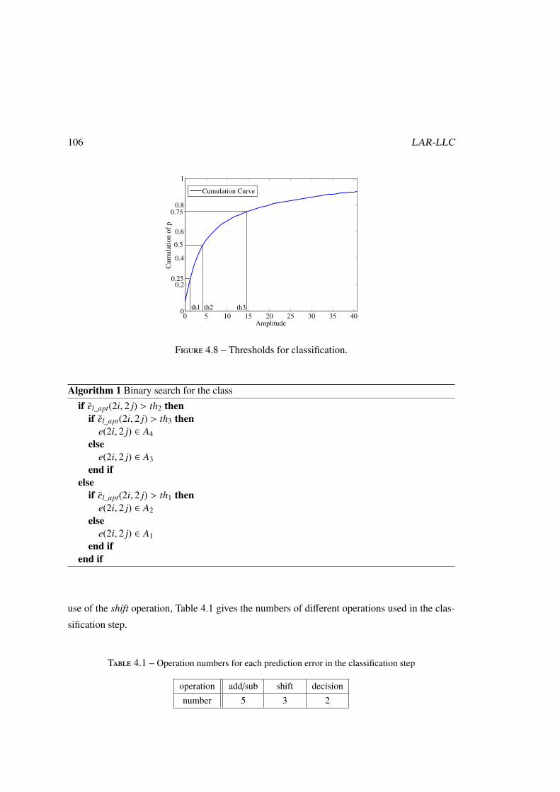
106 LAR-LLC
0 5 10 15 20 25 30 35 400
0.2
0.4
0.6
0.8
1
Amplitude
Cu
mu
lati
on
of
p
Cumulation Curve
0.25
th2th1 th3
0.75
0.5
Figure 4.8 – Thresholds for classification.
Algorithm 1 Binary search for the classif el_apt(2i, 2 j) > th2 then
if el_apt(2i, 2 j) > th3 thene(2i, 2 j) ∈ A4
elsee(2i, 2 j) ∈ A3
end ifelse
if el_apt(2i, 2 j) > th1 thene(2i, 2 j) ∈ A2
elsee(2i, 2 j) ∈ A1
end ifend if
use of the shift operation, Table 4.1 gives the numbers of different operations used in the clas-
sification step.
Table 4.1 – Operation numbers for each prediction error in the classification step
operation add/sub shift decision
number 5 3 2

Compression Performance 107
-40 -30 -20 -10 0 10 20 30 400
0.05
0.1
0.15
Data
De
nsity
subsequence A1subsequence A2subsequence A3subsequence A4original error of G1
originalerror of G1
Figure 4.9 – Distributions of subsequences and original error sequence of G1 on image “bike”.
4.5 Compression Performance
In this section, the effectiveness of the proposed LAR-LLC is compared with those of still
image compression standards in compression efficiency and coding speed. These standards
are still current references for image coding and their complete reference solutions are avai-
lable : the JPEG2000 (JPEG2K) implementation is available in [Ada] ; the JPEGXR reference
software is generated from [ITU] ; JPEGLS is from [UBC] and Lossless JPEG is offered in
[HS]. Because this work focuses on the complexity, although some other image coding me-
thods report better compression ratios with heavier computations, they are not compared in
detail in this section. Kim et al. proposed a hierarchical prediction and context adaptive coding
for lossless color image compression (LCIC) [KC14]. They offered the reference execution
[KC]. They pointed out that their coding method LCIC can show an average bit rate reduc-
tion over JPEG2K, but it needs slightly more computation time than JPEG2K. Therefore, we
also take this referenced method into the comparison. 16 images (RGB 24 bit/pixel) with dif-
ferent content/features are chosen mainly from the set of ISO/ITU reference images. They cover
contents of objects, human and surrounding views. Test images are presented in Fig.4.10.
4.5.1 Compression Efficiency
This subsection firstly shows the effectiveness of the classification scheme used in the Pre-
coding part. Table 4.2 gives the entropy reduction of the prediction error stream G1 of each
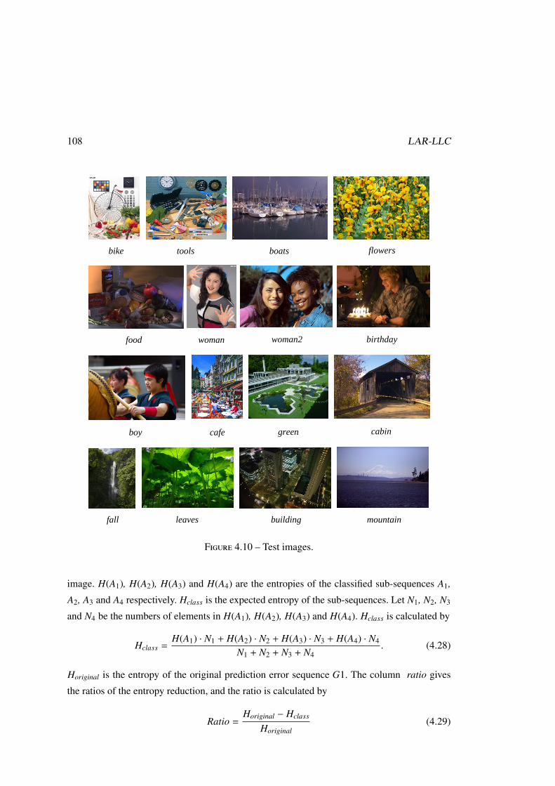
108 LAR-LLC
x
a b
c
bike tools boats flowers food woman woman2 birthday
boy cafe green cabin fall leaves building mountain
bike tools boats flowers
food woman woman2 birthday
boy cafe green cabin
fall leaves building mountain
Figure 4.10 – Test images.
image. H(A1), H(A2), H(A3) and H(A4) are the entropies of the classified sub-sequences A1,
A2, A3 and A4 respectively. Hclass is the expected entropy of the sub-sequences. Let N1, N2, N3
and N4 be the numbers of elements in H(A1), H(A2), H(A3) and H(A4). Hclass is calculated by
Hclass =H(A1) · N1 + H(A2) · N2 + H(A3) · N3 + H(A4) · N4
N1 + N2 + N3 + N4. (4.28)
Horiginal is the entropy of the original prediction error sequence G1. The column ratio gives
the ratios of the entropy reduction, and the ratio is calculated by
Ratio =Horiginal − Hclass
Horiginal(4.29)
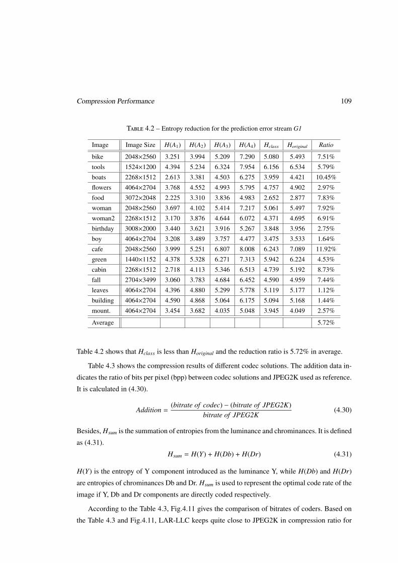
Compression Performance 109
Table 4.2 – Entropy reduction for the prediction error stream G1
Image Image Size H(A1) H(A2) H(A3) H(A4) Hclass Horiginal Ratio
bike 2048×2560 3.251 3.994 5.209 7.290 5.080 5.493 7.51%
tools 1524×1200 4.394 5.234 6.324 7.954 6.156 6.534 5.79%
boats 2268×1512 2.613 3.381 4.503 6.275 3.959 4.421 10.45%
flowers 4064×2704 3.768 4.552 4.993 5.795 4.757 4.902 2.97%
food 3072×2048 2.225 3.310 3.836 4.983 2.652 2.877 7.83%
woman 2048×2560 3.697 4.102 5.414 7.217 5.061 5.497 7.92%
woman2 2268×1512 3.170 3.876 4.644 6.072 4.371 4.695 6.91%
birthday 3008×2000 3.440 3.621 3.916 5.267 3.848 3.956 2.75%
boy 4064×2704 3.208 3.489 3.757 4.477 3.475 3.533 1.64%
cafe 2048×2560 3.999 5.251 6.807 8.008 6.243 7.089 11.92%
green 1440×1152 4.378 5.328 6.271 7.313 5.942 6.224 4.53%
cabin 2268×1512 2.718 4.113 5.346 6.513 4.739 5.192 8.73%
fall 2704×3499 3.060 3.783 4.684 6.452 4.590 4.959 7.44%
leaves 4064×2704 4.396 4.880 5.299 5.778 5.119 5.177 1.12%
building 4064×2704 4.590 4.868 5.064 6.175 5.094 5.168 1.44%
mount. 4064×2704 3.454 3.682 4.035 5.048 3.945 4.049 2.57%
Average 5.72%
Table 4.2 shows that Hclass is less than Horiginal and the reduction ratio is 5.72% in average.
Table 4.3 shows the compression results of different codec solutions. The addition data in-
dicates the ratio of bits per pixel (bpp) between codec solutions and JPEG2K used as reference.
It is calculated in (4.30).
Addition =(bitrate of codec) − (bitrate of JPEG2K)
bitrate of JPEG2K(4.30)
Besides, Hsum is the summation of entropies from the luminance and chrominances. It is defined
as (4.31).
Hsum = H(Y) + H(Db) + H(Dr) (4.31)
H(Y) is the entropy of Y component introduced as the luminance Y, while H(Db) and H(Dr)
are entropies of chrominances Db and Dr. Hsum is used to represent the optimal code rate of the
image if Y, Db and Dr components are directly coded respectively.
According to the Table 4.3, Fig.4.11 gives the comparison of bitrates of coders. Based on
the Table 4.3 and Fig.4.11, LAR-LLC keeps quite close to JPEG2K in compression ratio for
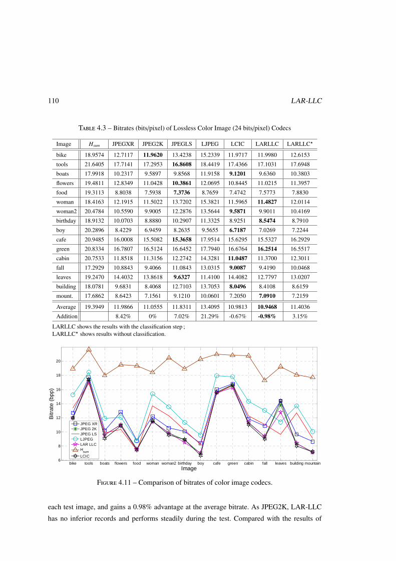
110 LAR-LLC
Table 4.3 – Bitrates (bits/pixel) of Lossless Color Image (24 bits/pixel) Codecs
Image Hsum JPEGXR JPEG2K JPEGLS LJPEG LCIC LARLLC LARLLC?
bike 18.9574 12.7117 11.9620 13.4238 15.2339 11.9717 11.9980 12.6153
tools 21.6405 17.7141 17.2953 16.8608 18.4419 17.4366 17.1031 17.6948
boats 17.9918 10.2317 9.5897 9.8568 11.9158 9.1201 9.6360 10.3803
flowers 19.4811 12.8349 11.0428 10.3861 12.0695 10.8445 11.0215 11.3957
food 19.3113 8.8038 7.5938 7.3736 8.7659 7.4742 7.5773 7.8830
woman 18.4163 12.1915 11.5022 13.7202 15.3821 11.5965 11.4827 12.0114
woman2 20.4784 10.5590 9.9005 12.2876 13.5644 9.5871 9.9011 10.4169
birthday 18.9132 10.0703 8.8880 10.2907 11.3325 8.9251 8.5474 8.7910
boy 20.2896 8.4229 6.9459 8.2635 9.5655 6.7187 7.0269 7.2244
cafe 20.9485 16.0008 15.5082 15.3658 17.9514 15.6295 15.5327 16.2929
green 20.8334 16.7807 16.5124 16.6452 17.7940 16.6764 16.2514 16.5517
cabin 20.7533 11.8518 11.3156 12.2742 14.3281 11.0487 11.3700 12.3011
fall 17.2929 10.8843 9.4066 11.0843 13.0315 9.0087 9.4190 10.0468
leaves 19.2470 14.4032 13.8618 9.6327 11.4100 14.4082 12.7797 13.0207
building 18.0781 9.6831 8.4068 12.7103 13.7053 8.0496 8.4108 8.6159
mount. 17.6862 8.6423 7.1561 9.1210 10.0601 7.2050 7.0910 7.2159
Average 19.3949 11.9866 11.0555 11.8311 13.4095 10.9813 10.9468 11.4036
Addition 8.42% 0% 7.02% 21.29% -0.67% -0.98% 3.15%
LARLLC shows the results with the classification step ;LARLLC? shows results without classification.
bike tools boats flowers food woman woman2 birthday boy cafe green cabin fall leaves building mountain
6
8
10
12
14
16
18
20
Image
Bitr
ate
(bpp
)
JPEG XRJPEG 2KJPEG LSLJPEGLAR LLCHsumLCIC
Figure 4.11 – Comparison of bitrates of color image codecs.
each test image, and gains a 0.98% advantage at the average bitrate. As JPEG2K, LAR-LLC
has no inferior records and performs steadily during the test. Compared with the results of
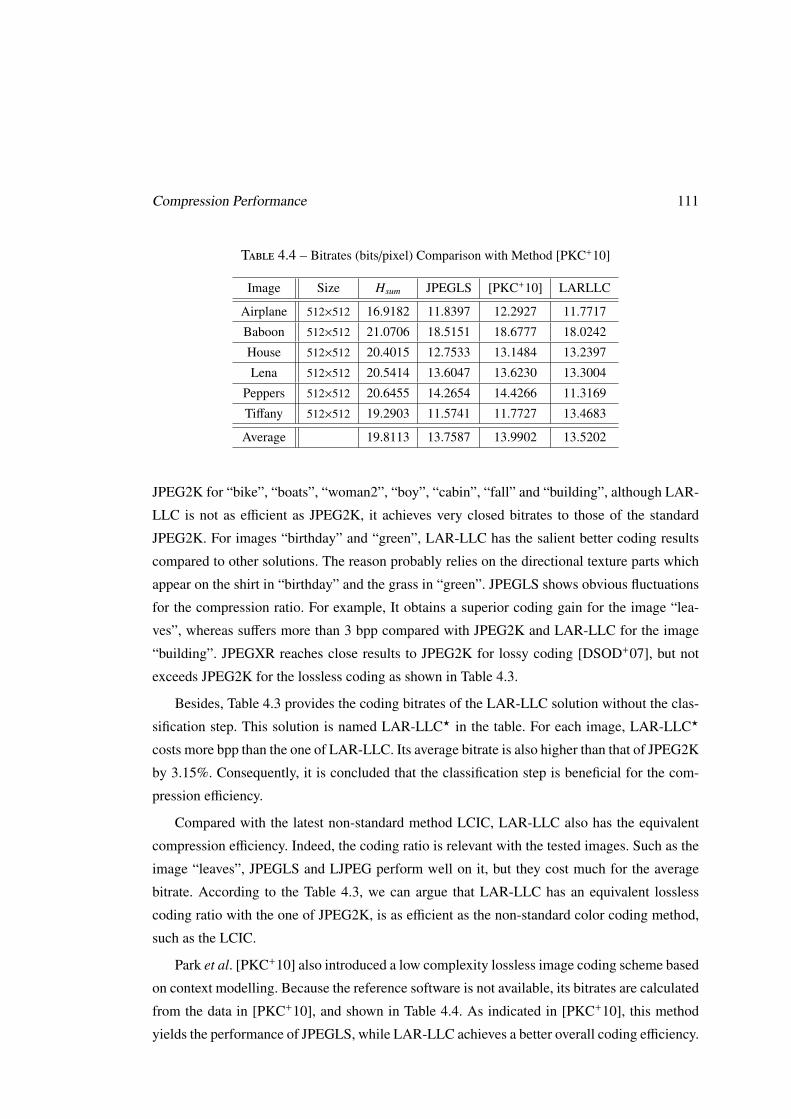
Compression Performance 111
Table 4.4 – Bitrates (bits/pixel) Comparison with Method [PKC+10]
Image Size Hsum JPEGLS [PKC+10] LARLLC
Airplane 512×512 16.9182 11.8397 12.2927 11.7717
Baboon 512×512 21.0706 18.5151 18.6777 18.0242
House 512×512 20.4015 12.7533 13.1484 13.2397
Lena 512×512 20.5414 13.6047 13.6230 13.3004
Peppers 512×512 20.6455 14.2654 14.4266 11.3169
Tiffany 512×512 19.2903 11.5741 11.7727 13.4683
Average 19.8113 13.7587 13.9902 13.5202
JPEG2K for “bike”, “boats”, “woman2”, “boy”, “cabin”, “fall” and “building”, although LAR-
LLC is not as efficient as JPEG2K, it achieves very closed bitrates to those of the standard
JPEG2K. For images “birthday” and “green”, LAR-LLC has the salient better coding results
compared to other solutions. The reason probably relies on the directional texture parts which
appear on the shirt in “birthday” and the grass in “green”. JPEGLS shows obvious fluctuations
for the compression ratio. For example, It obtains a superior coding gain for the image “lea-
ves”, whereas suffers more than 3 bpp compared with JPEG2K and LAR-LLC for the image
“building”. JPEGXR reaches close results to JPEG2K for lossy coding [DSOD+07], but not
exceeds JPEG2K for the lossless coding as shown in Table 4.3.
Besides, Table 4.3 provides the coding bitrates of the LAR-LLC solution without the clas-
sification step. This solution is named LAR-LLC? in the table. For each image, LAR-LLC?
costs more bpp than the one of LAR-LLC. Its average bitrate is also higher than that of JPEG2K
by 3.15%. Consequently, it is concluded that the classification step is beneficial for the com-
pression efficiency.
Compared with the latest non-standard method LCIC, LAR-LLC also has the equivalent
compression efficiency. Indeed, the coding ratio is relevant with the tested images. Such as the
image “leaves”, JPEGLS and LJPEG perform well on it, but they cost much for the average
bitrate. According to the Table 4.3, we can argue that LAR-LLC has an equivalent lossless
coding ratio with the one of JPEG2K, is as efficient as the non-standard color coding method,
such as the LCIC.
Park et al. [PKC+10] also introduced a low complexity lossless image coding scheme based
on context modelling. Because the reference software is not available, its bitrates are calculated
from the data in [PKC+10], and shown in Table 4.4. As indicated in [PKC+10], this method
yields the performance of JPEGLS, while LAR-LLC achieves a better overall coding efficiency.
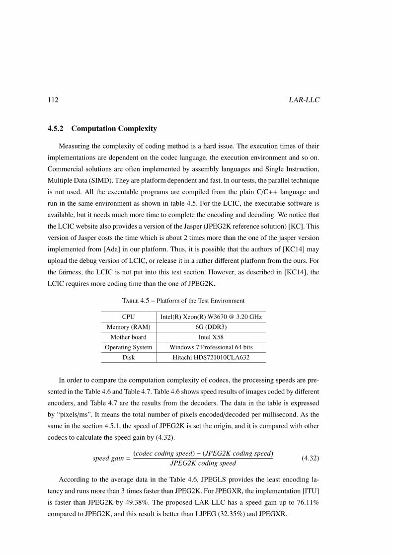
112 LAR-LLC
4.5.2 Computation Complexity
Measuring the complexity of coding method is a hard issue. The execution times of their
implementations are dependent on the codec language, the execution environment and so on.
Commercial solutions are often implemented by assembly languages and Single Instruction,
Multiple Data (SIMD). They are platform dependent and fast. In our tests, the parallel technique
is not used. All the executable programs are compiled from the plain C/C++ language and
run in the same environment as shown in table 4.5. For the LCIC, the executable software is
available, but it needs much more time to complete the encoding and decoding. We notice that
the LCIC website also provides a version of the Jasper (JPEG2K reference solution) [KC]. This
version of Jasper costs the time which is about 2 times more than the one of the jasper version
implemented from [Ada] in our platform. Thus, it is possible that the authors of [KC14] may
upload the debug version of LCIC, or release it in a rather different platform from the ours. For
the fairness, the LCIC is not put into this test section. However, as described in [KC14], the
LCIC requires more coding time than the one of JPEG2K.
Table 4.5 – Platform of the Test Environment
CPU Intel(R) Xeon(R) W3670 @ 3.20 GHz
Memory (RAM) 6G (DDR3)
Mother board Intel X58
Operating System Windows 7 Professional 64 bits
Disk Hitachi HDS721010CLA632
In order to compare the computation complexity of codecs, the processing speeds are pre-
sented in the Table 4.6 and Table 4.7. Table 4.6 shows speed results of images coded by different
encoders, and Table 4.7 are the results from the decoders. The data in the table is expressed
by “pixels/ms”. It means the total number of pixels encoded/decoded per millisecond. As the
same in the section 4.5.1, the speed of JPEG2K is set the origin, and it is compared with other
codecs to calculate the speed gain by (4.32).
speed gain =(codec coding speed) − (JPEG2K coding speed)
JPEG2K coding speed(4.32)
According to the average data in the Table 4.6, JPEGLS provides the least encoding la-
tency and runs more than 3 times faster than JPEG2K. For JPEGXR, the implementation [ITU]
is faster than JPEG2K by 49.38%. The proposed LAR-LLC has a speed gain up to 76.11%
compared to JPEG2K, and this result is better than LJPEG (32.35%) and JPEGXR.
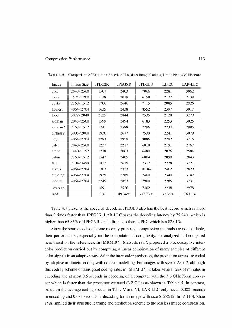
Compression Performance 113
Table 4.6 – Comparison of Encoding Speeds of Lossless Image Codecs, Unit : Pixels/Millisecond
Image Image Size JPEG2K JPEGXR JPEGLS LJPEG LAR-LLC
bike 2048×2560 1507 2403 7066 2281 3062
tools 1524×1200 1138 2019 6158 2177 2438
boats 2268×1512 1706 2646 7115 2085 2926
flowers 4064×2704 1635 2438 8552 2397 3017
food 3072×2048 2125 2844 7535 2128 3279
woman 2048×2560 1599 2494 6183 2253 3025
woman2 2268×1512 1741 2588 7296 2234 2985
birthday 3008×2000 1936 2677 7539 2241 3079
boy 4064×2704 2283 2959 8086 2292 3215
cafe 2048×2560 1237 2217 6818 2191 2767
green 1440×1152 1218 2063 6480 2076 2584
cabin 2268×1512 1547 2485 6804 2090 2843
fall 2704×3499 1822 2615 7317 2278 3221
leaves 4064×2704 1383 2323 10184 2462 2829
building 4064×2704 1935 2785 7400 2340 3142
mount. 4064×2704 2245 2853 7900 2285 3231
Average 1691 2526 7402 2238 2978
Add. 0% 49.38% 337.73% 32.35% 76.11%
Table 4.7 presents the speed of decoders. JPEGLS also has the best record which is more
than 2 times faster than JPEG2K. LAR-LLC saves the decoding latency by 75.94% which is
higher than 65.85% of JPEGXR, and a little less than LJPEG which has 82.01%.
Since the source codes of some recently proposed compression methods are not available,
their performances, especially on the computational complexity, are analyzed and compared
here based on the references. In [MKMI07], Matsuda et al. proposed a block-adaptive inter-
color prediction carried out by computing a linear combination of many samples of different
color signals in an adaptive way. After the inter-color prediction, the prediction errors are coded
by adaptive arithmetic coding with context modelling. For images with size 512×512, although
this coding scheme obtains good coding rates in [MKMI07], it takes several tens of minutes in
encoding and at most 0.5 seconds in decoding on a computer with the 3.6 GHz Xeon proces-
sor which is faster than the processor we used (3.2 GHz) as shown in Table 4.5. In contrast,
based on the average coding speeds in Table V and VI, LAR-LLC only needs 0.088 seconds
in encoding and 0.081 seconds in decoding for an image with size 512×512. In [ZH10], Zhao
et al. applied their structure learning and prediction scheme to the lossless image compression.
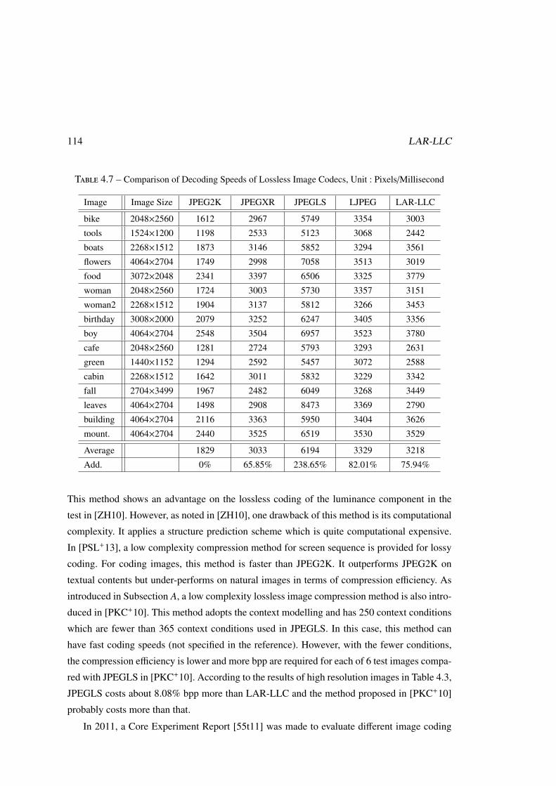
114 LAR-LLC
Table 4.7 – Comparison of Decoding Speeds of Lossless Image Codecs, Unit : Pixels/Millisecond
Image Image Size JPEG2K JPEGXR JPEGLS LJPEG LAR-LLC
bike 2048×2560 1612 2967 5749 3354 3003
tools 1524×1200 1198 2533 5123 3068 2442
boats 2268×1512 1873 3146 5852 3294 3561
flowers 4064×2704 1749 2998 7058 3513 3019
food 3072×2048 2341 3397 6506 3325 3779
woman 2048×2560 1724 3003 5730 3357 3151
woman2 2268×1512 1904 3137 5812 3266 3453
birthday 3008×2000 2079 3252 6247 3405 3356
boy 4064×2704 2548 3504 6957 3523 3780
cafe 2048×2560 1281 2724 5793 3293 2631
green 1440×1152 1294 2592 5457 3072 2588
cabin 2268×1512 1642 3011 5832 3229 3342
fall 2704×3499 1967 2482 6049 3268 3449
leaves 4064×2704 1498 2908 8473 3369 2790
building 4064×2704 2116 3363 5950 3404 3626
mount. 4064×2704 2440 3525 6519 3530 3529
Average 1829 3033 6194 3329 3218
Add. 0% 65.85% 238.65% 82.01% 75.94%
This method shows an advantage on the lossless coding of the luminance component in the
test in [ZH10]. However, as noted in [ZH10], one drawback of this method is its computational
complexity. It applies a structure prediction scheme which is quite computational expensive.
In [PSL+13], a low complexity compression method for screen sequence is provided for lossy
coding. For coding images, this method is faster than JPEG2K. It outperforms JPEG2K on
textual contents but under-performs on natural images in terms of compression efficiency. As
introduced in Subsection A, a low complexity lossless image compression method is also intro-
duced in [PKC+10]. This method adopts the context modelling and has 250 context conditions
which are fewer than 365 context conditions used in JPEGLS. In this case, this method can
have fast coding speeds (not specified in the reference). However, with the fewer conditions,
the compression efficiency is lower and more bpp are required for each of 6 test images compa-
red with JPEGLS in [PKC+10]. According to the results of high resolution images in Table 4.3,
JPEGLS costs about 8.08% bpp more than LAR-LLC and the method proposed in [PKC+10]
probably costs more than that.
In 2011, a Core Experiment Report [55t11] was made to evaluate different image coding
Conclusion 115
methods. The original LAR method is about 2 times slower than JPEG2K in both encoding
and decoding during tests. It encouraged the design of a new low complexity solution. LAR-
LLC can achieve the equivalent lossless compression efficiency of JPEG2K, while be 76.11%
faster than JPEG2K for encoding and 75.94% faster for decoding. JPEGLS has the least time
consumption on coding. However, it costs 7.02% bpp more than JPEG2K and about 8.08%
more than LAR-LLC, and has fluctuations for the compression ratio compared with LAR-
LLC. LAR-LLC has less coding latency than JPEGXR, and saves 8.67% bpp of JPEGXR.
Besides, LAR-LLC also supports the spatial scalability as JPEG2K does for multi-resolution
application.
The LAR-LLC currently runs in a mono thread configuration, but has potential parallel
processing ability in multi-threading. For the pyramid building process in Section 4.2, the DC
component for blocks at each level is independently estimated. Then, the global process can
be performed in a SIMD approach, with one thread processing one part of the image. Besides,
during the pyramidal decomposition, the image coding process involves three main pipelined
steps : prediction, classification and Huffman coding. These stages are performed for each level
and for three coefficients per level. It means that the last Huffman coding step in level l + 1 can
run simultaneously with the prediction step in level l, both handled by different threads. Some
parallel processing is also possible for JPEG2K for the Discrete Wavelet Transform (DWT)
part [SJ09] or the EBCOT module [MOS11]. Recently, new parallel processing methods and
advanced graphic processing units are also applied to JPEG2K for a significant speedup in the
execution time [LBM11][WCL12].
4.6 Conclusion
In this chapter, a low complexity scalable lossless image compression method LAR-LLC
is introduced to decrease the latency of encoding and decoding while remaining high compres-
sion efficiency. Based on a Hierarchical Diagonal S Transform, coding starts at a top-down
dyadic decomposition with targeted prediction processes. For each process, the predictor runs
in one pass and avoids the latency caused by the feedback action. Because the prediction errors
are coded from the low resolution to the full resolution level, this coding structure offers the
scalable resolution ability in the bit stream. The receiving terminal can decode the image in
progressive-resolution according to the channel capacity and user requirements. After the pre-
diction, a classification step is applied to reduce the entropy of prediction errors for increasing
the coding efficiency.
116 LAR-LLC
Experiments showed that, the pre-coding scheme including the classification action really
decreases the entropy of the error sequence, and it is beneficial for the following entropy co-
ding step. For the lossless coding of the nature color images, LAR-LLC achieves the coding
efficiency equivalent to JPEG2K, and as good as the latest non-standard coding method. Be-
sides, LAR-LLC has less coding latency in both encoding and decoding parts than the ones of
JPEG2K. Due to the space scalability, low complexity and notable compression ratio, LAR-
LLC is a good image compression solution with high quality for the multimedia storage and
communication, implementing both in hardware and in software.
Chapter 5
Conclusion and Perspectives
In this manuscript we introduced a RDO (Rate-distortion-optimization) model, an objec-
tive quality control model and an enhancement scheme of the subjective quality for the lossy
coding based on LAR the (Locally Adaptive Resolution) image codec. Besides, a new lossless
image codec, LAR-LLC (Locally-adaptive resolution, lossless low complexity), is introduced
to achieve a coding efficiency equivalent to that of JPEG2000, while having a lower computa-
tional complexity in order to reduce the coding latency. The contributions of the novelties are
presented in the conclusion section in detail.
5.1 Conclusion of the thesis work
5.1.1 Rate-distortion-optimization model for LAR codec
The classic LAR codec has complete lossy and lossless coding structures. In the lossy
coding mode, two functions, the Quadtree partitioning and the quantization of the prediction
errors, are designed to miss the information of the image in order to economize the bitrate.
Meanwhile, the Quadtree partition is controlled by a threshold Thr, and the Quantization is
regulated by a parameter quqp. The study firstly analysed the different distortions derived from
the Thr and the quqp, next selected the optimal pairs of the Thr and the quqp. Based on the
characters of adjacent pixels, a RDO model is built to describe the relationship of the Thr and
the quqp of the optimal pairs. According to the model, a suitable Thr corresponding to a set
quqp can be chosen. With the modeled Thr and quqp, the LAR codec can achieve an optimal
or closely optimal lossy coding efficiency. The RDO model is introduced in Section 3.2.
By the use of the RDO model, the Mean Square Error (MSE) of the decoded image shows
117
118 Conclusion and Perspectives
a nearly linear relationship with the quqp. Therefore, a linear model is proposed to describe
this relationship. With this linear model, users can refrain the overall distortion of the decoded
image to a target MSE by a choice of quqp. This part is introduced in Subsection 3.4.1.
Moreover, because the RDO model is sensitive to the change of pixels, it is used in adjacent
regions in order to allocate a series of Thr which is adaptive to local change of pixels. This
allocation meets the fact that the human visual system is less sensitive to noise in strong texture
areas than the less textured areas. After this adaptive Thr allocation, the decoded image has
a better perceptual quality and higher subjective score measured by the Structure Similarity
(SSIM) than the one without the allocation scheme. Meanwhile, this allocation scheme brings
a little influence on the objective quality measured by the Peak signal-to-noise ratio (PSNR).
The relative analysis is given in Section 3.5.
5.1.2 Lossless Low-complexity codec LAR-LLC
Due to the limited compression efficiency and high computational complexity, the classic
LAR codec shows a lower performance than that of the standard JPEG2000. In Chapter 4, a
new lossless image coding method LAR-LLC which is based on the LAR framework is intro-
duced. This method still supports the multi-resolution function which is realized by a HD-ST
Transform. This transform is reversible and easy to be implemented. The coding process is
similar with the classic LAR codec, and starts from the lowest resolution level. It uses the cor-
relation of intra and inter levels to reconstruct higher resolution images, until the full resolution
image is achieved. The reconstruction procedure depends on three prediction steps. The predic-
tion errors need to be coded for the decoder to recover the image. The prediction errors should
be lossless coded. In order to improve the compression efficiency of the entropy coders for the
prediction errors, a pre-coding step is added to reduce the entropy of the error sequence. The
experiments are introduced in Subsection 4.5.1. The experimental results firstly confirm that
the pre-coding step decreases the entropy of the sequence of the prediction errors, next, accor-
ding to the comparison of different codecs on the compression efficiency, LAR-LLC shows an
equivalent performance to the one of JPEG2000 : the average bitrate of LAR-LLC is 0.98%
less than the one of JPEG2000, this result is a little better than the one (0.67%) of the codec
derived from the recent proposed lossless image coing method LCIC [KC14]. LAR-LLC also
has relative stable compression ratios as JPEG2000 does in the comparison with JPEGLS. In
the complexity test, LAR-LLC shows the less coding latency than JPEG2000 : 76.11% faster
than JPEG2000 in the encoding and 75.94% in the decoding.
Perspectives 119
5.2 Perspectives
This section presents some ideas that could be prospects of the future research. These ideas
are derived from the study of the LAR, and could be benefit for other image codecs or data
compression techniques.
5.2.1 Distortion control based on the perceptual quality in the lossy coding
The metrics of the objective quality are still the most widely used methods to evaluate the
decoded images. They can detect any distortions in the reconstructed image and give corres-
ponding quality “scores” for the image. Many lossy coding methods aim at the reduction of
the objective distortion, and design their RDO and rate control (RC) schemes. However, this
strategy is not suitable in some cases for the natural images. Although some kinds of distortions
may reduce largely the objective quality, such as PSNR, they do not bring much visible uncom-
fortable effects to the decoded image, as examples discussed in Section 3.5. A human viewer
is the final judge of the image quality in most applications, therefore, it is advantageous to take
into account the properties and characteristics of the Human Visual System (HVS) that affect
the image quality as judged by human viewers when one is designing an image compression
algorithm and assessing picture quality.
The objective quality measures are mainly used because of their simple analysis and the
lack of other available and accepted standardized quality measures [EF95] [SF96]. Meanw-
hile, for the subjective measurement, the images are often rated based on the visibility of the
distortion artefacts according to a predetermined scale [SF96]. Although the test is reliable, it
requires specialized viewing conditions [CLCB03] and can not be used as a real-time scheme to
improve the coding. There has been considerable amount of research done to develop objective
metrics which incorporate the perceived quality measurement by considering HVS characteris-
tics [SF96], [GMK02], [WBSS04]. Similarly, for the LAR codec, it is possible to modify the
lossy coding under the consideration of the perceived quality. As described in Chapter 3, the
RDO model is derived from the analysis on the objective distortion measurement. The subjec-
tive enhancement scheme has been based on the fact that the edge lying in a textured region is
less visible to a human observer compared to the edge in a plain background.
In the future work, another factor needs to be considered for the visual sensitivity is the
background luminance : the visibility of the edge is often affected by the surrounding regions.
For example, the edge lying in a darker region is less visible compared to the edge in the
brighter region [KK95] [VBP05]. It indicates that the distortion in the dark region is more
120 Conclusion and Perspectives
tolerable than the one in the bright region. Therefore, it is more important to record the changes
of pixels in the plain and bright region rather than in the textured and darker region. Take the
Fig.3.34 as an example, with the adaptive Thr allocation scheme, the Quadtree grid uses small
blocks to reserve the details on the face and hand, but in the hair and the gray background, the
Quadtree grid does not need to allocate a lot of small blocks to record the changes of pixels.
This idea requires a luminance detection before the adaptive Thr allocation. For the dark region,
a fixed Thr is directly applied to the Quadtree partition. It can be seen as an extension of the
locally adaptive Thr allocation scheme in order to modify the Thr map.
Moreover, in the future work, the distortion derived from the quantization needs to be
controlled. As indicated in Subsection 3.5.1, the magnitude of a justly noticeable luminance
change ∆I is approximately proportional to the background luminance I for a wide range of
the luminance values. In the quantization step, the difference between the original pixel and the
de-quantized one is weighted by the Weber’s law as did in [WB06] [TVDY12].
5.2.2 Better context model for the classification in the Pre-coding process
Section 4.4 introduced a forward classification scheme in order to reduce the entropy of the
prediction error stream. It also indicates that if the two subclasses have no intersections, and
the same length, the average code length can reach H(A) − 1. Therefore, the accuracy of the
classification affects the final average code length. The proposed context model, shown in Fig.
4.7 and Eq. (4.26), can differ the probability distribution of subclasses as shown in Fig. 4.9.
This model has accurate rates about 60% to 70% in the tests. The entropy coding efficiency
can be enhanced with a higher accuracy. One possible method is to build a context model
set and choose a suitable model adaptively during the classification. This method requires a
local analysis on the direction of pixels in order to decide which prediction error, such as
el(2i− 2, 2 j− 2), el(2i, 2 j− 2), el(2i + 2, 2 j− 2), el(2i− 2, 2 j) and el+1(i, j), should has a higher
weight. Indeed, more latency of the coding is caused by this analysis.
Another solution is to use a data sequence to record the information of the accurate clas-
sification. This side sequence needs to be coded. Notice that the side sequence has a very li-
mited alphabet, the symbols probability repeats frequently. A Run-length plus Huffman coding
is considered to code this side information. The run-length coding generates the successive
symbols onto one new symbol and the sequence the new generated symbols is coded by the
Huffman coding. The total entropy is not reduced, but the side information sequence is quite
simple to achieve an efficient coding ratio.
Glossary
p(x) the probability of occurrence of the symbol x
H(X) the entropy of the alphabet set X
H(X|Y) the conditional entropy, the uncertainty of X when Y has been known
DCT the Discrete Cosine Transform
DWT the Discrete Wavelet Transform
VLC the variable length coding
Thr the threshold used for the Quadtree Partition
I(x, y) the pixel of an image in the position (x, y)
b.c rounding downward
1M the Image made of the mean value of the first diagonal by S transform
2G the Image made of the gradient value of the first diagonal by S transform
3M the Image made of the mean value of the second diagonal by S transform
3G the Image made of the gradient value of the second diagonal by S transform
2G the predicted image of 2G
3M the predicted image of 3M
3G the predicted image of 3G
quqp the global quantization factor
RDO rate distortion optimization
QC quality control
121

122 Glossary
RC rate control
MSE Mean Square Error
PSNR Peak Signal-to-noise Ratio
r(i) the cumulation of the probabilities
MSEest the estimated MSE
MSEset the target MSE
HVS Human Visual System
SSIM Structural Similarity
MSSIM mean SSIM
Yl(i, j) the pixel on the position (i,j) in the level l
M1,l the mean value of the first diagonal in the block of the level l
G1,l the gradient value of the first diagonal in the block of the level l
M2,l the mean value of the second diagonal in the block of the level l
G2,l the gradient value of the second diagonal in the block of the level l
Md,l the mean value of the block in the level l
Gd,l the difference value of M1,l and M2,l in the level l
Gd,l the predicted value of Gd,l
G1,l the predicted value of G1,l
G2,l the predicted value of G2,l
∪ the union
∩ the intersection
∅ the null set
e the prediction error
SIMD Single Instruction, Multiple Data
Publication
“LAR-LLC : A Low Complexity Multiresolution Lossless Image Codec”, Liu Y., Deforges O.,
Samrouth K., IEEE Trans. on Circuits and Systems for Video Technology, resubmitted after
major revision for review.
“Autofocus on Depth of Interest for 3D image coding”, Samrouth K., Deforges O., Liu Y.,
Khalil M., Falou W., EURASIP Journal on Image and Video Processing, submitted.
“A Joint 3D Image Semantic Segmentation and Scalable Coding Scheme with ROI Approach”,
Samrouth K., Deforges O., Liu Y., Khalil M., Falou W., IEEE Visual Communications and
Image Processing (IEEE VCIP), Dec. 2014.
“One Pass Quality Control and Low Complexity RDO in A Quadtree Based Scalable Image
Coder”, Liu Y., Deforges O., Pasteau F., Samrouth K., 2013 IEEE Second International Confe-
rence on Image Information Processing, Best paper, pp. 187-192, Dec. 2013.
“Low Complexity RDO Model for Locally Subjective Quality Enhancement in LAR Coder”,
Liu Y., Déforges O., Pasteau F., Samrouth K., IEEE International Conference on Signal and
Image Processing Applications (ICSIPA), pp.176-181, Oct. 2013.
“Efficient Depth Map Compression Exploiting Correlation with Texture Data in Multiresolu-
tion Predictive Image Coders”, Samrouth K., Deforges O., Liu Y., Pasteau F., Khalil M., Falou
W., 2013 IEEE International Conference on Multimedia and Expo Workshops (ICMEW), Hot
topics in 3D coding, pp.1-6, Jul. 2013.
123

124 Publication
Bibliography
[55t11] Meeting report, 55th meeting of ISO/IEC JTC 1/SC 29/WG 1. Technical Report
N5880, Jul. 2011.
[ABMD92] M. Antonini, M. Barlaud, P. Mathieu, and I. Daubechies. Image coding using
wavelet transform. IEEE Transactions on Image Processing, 1(2) :205–220,
Apr 1992.
[Ada] Michael Adams. The jasper project for JPEG 2000 part-1 standard. http ://
www.ece.uvic.ca/ frodo/ jasper/.
[Ash01] Michael Ashikhmin. Synthesizing natural textures. In Proceedings of the 2001
Symposium on Interactive 3D Graphics, I3D ’01, pages 217–226, New York,
NY, USA, 2001. ACM.
[ASX] Beong-Jo Kim Amir Said, William A. Pearlman and Zixiang Xiong. SPIHT demo
programs. http :// www.cipr.rpi.edu/ research/ SPIHT/ spiht3.html.
[BD09] Marie Babel and Olivier Déforges. Response to call for aic technologies and eva-
luation methodologies. Technical Report wg1n4870, ISO/ITU JPEG commitee,
Jan. 2009.
[BD10] Marie Babel and Olivier Déforges. Response to call for aic evaluation metho-
dologies and compression technologies for medical images. Technical Report
wg1n5315, ISO/ITU JPEG commitee, Mar. 2010.
[BDR05] M. Babel, O. Déforges, and J. Ronsin. Interleaved s+p pyramidal decomposition
with refined prediction model. In IEEE International Conference on Image
Processing, volume 2, pages II–750–3, Sept 2005.
[CCI92] ITU CCITT. Information Technology - Digital Compression and Coding of
Continuous-tone still Images - Requirements and Guidelines. Technical Report
T.81, ITU and CCITT, Sept. 1992.
125
126 Bibliography
[CCX00] Chin-Chen Chang, Tung-Shou Chen, and Guang-Xue Xiao. An improved pre-
diction method for quadtree image coding. In International Symposium on
Multimedia Software Engineering, 2000. Proceedings, pages 269–275, 2000.
[CFC+06] Yu-Wei Chang, Hung-Chi Fang, Chih-Chi Cheng, Chun-Chia Chen, and Liang-
Gee Chen. Precompression quality-control algorithm for jpeg 2000. IEEE Tran-
sactions on Image Processing, 15(11) :3279–3293, Nov 2006.
[CH09] Jianle Chen and Woo Jin Han. Adaptive linear prediction for block-based lossy
image coding. In 16th IEEE International Conference on Image Processing
(ICIP), 2009, pages 2833–2836, Nov 2009.
[CK06] Fehmi Chebil and Ragip Kurceren. Pre-compression rate allocation for jpeg2000
encoders in power constrained devices, 2006.
[CLC08] Chun-Hsien Chou, Kuo-Cheng Liu, and Ping-Hsuan Chung. Perceptually opti-
mized rate control for jpeg2000 coding of color images. In CISP '08. Congress
on Image and Signal Processing, 2008, volume 2, pages 80–84, May 2008.
[CLCB03] M. Carnec, P. Le Callet, and D. Barba. An image quality assessment method
based on perception of structural information. In International Conference on
Image Processing, volume 3, pages III–185–8 vol.2, Sept 2003.
[CLHH09] Sao-Jie Chen, Guang-Huei Lin, Pao-Ann Hsiung, and Yu-Hen Hu. Hardware
Software Co-Design of a Multimedia SOC Platform. Springer Publishing
Company, Incorporated, 1st edition, 2009.
[DBBR07] O. Déforges, M. Babel, L. Bedat, and J. Ronsin. Color lar codec : A color image
representation and compression scheme based on local resolution adjustment and
self-extracting region representation. IEEE Transactions on Circuits and Sys-
tems for Video Technology, 17(8) :974–987, Aug. 2007.
[DBM06] Olivier Déforges, Marie Babel, and Jean Motsch. The RWHT+P for an improved
lossless multiresolution coding. In , page nc. EUSIPCO, 2006.
[DSOD+07] Francesca De Simone, Mourad Ouaret, Frederic Dufaux, Andrew G. Tescher,
and Touradj Ebrahimi. A comparative study of JPEG2000, AVC/H.264, and HD
photo, 2007.
[DWW+07] Wenpeng Ding, Feng Wu, Xiaolin Wu, Shipeng Li, and Houqiang Li. Adaptive
directional lifting-based wavelet transform for image coding. IEEE Transac-
tions on Image Processing, 16(2) :416–427, Feb 2007.
Bibliography 127
[EB98] Michael P. Eckert and Andrew P. Bradley. Perceptual quality metrics applied to
still image compression. Signal Processing, 70(3) :177 – 200, 1998.
[ECW04] Farzad Ebrahimi, Matthieu Chamik, and Stefan Winkler. Jpeg vs. jpeg2000 :
An objective comparison of image encoding quality. In Proceedings of SPIE
Applications of Digital Image Processing, page 300308, 2004.
[EF95] A.M. Eskicioglu and P.S. Fisher. Image quality measures and their performance.
IEEE Transactions on Communications, 43(12) :2959–2965, Dec 1995.
[GMK02] Wenfeng Gao, C. Mermer, and Yongmin Kim. A de-blocking algorithm and a
blockiness metric for highly compressed images. IEEE Transactions on Cir-
cuits and Systems for Video Technology, 12(12) :1150–1159, Dec 2002.
[Gro] Independent JPEG Group. library for JPEG codec. http :// www.ijg.org/.
[GZ08] Zhigang Gao and Y.F. Zheng. Quality constrained compression using DWT-
Based image quality metric. IEEE Transactions on Circuits and Systems
for Video Technology, 18(7) :910–922, July 2008.
[HDG92] Y. Huang, H. Dreizen, and N.P. Galatsanos. Prioritized DCT for compression and
progressive transmission of images. IEEE Transactions on Image Processing,
1(4) :477–487, Oct 1992.
[HS] Kongji Huang and Brian Smith. LJPEG Software. ftp :// ftp.cs.cornell.edu/ pub/
multimed/.
[ISO09] ISO/IEC. JPEG XR image coding system – Part 2 : Image coding specification.
Technical Report ISO/IEC 29199-2 :2009, ISO, Jun. 2009.
[IT98] ITU-T. Information technology - Lossless and near-lossless compression of
continuous-tone still images -Baseline. Technical Report T.87, ITU-T, Jun. 1998.
[IT02] ITU-T. Information technology - JPEG 2000 image coding system : Core coding
system. Technical Report T.800, ITU-T, Aug. 2002.
[ITU] ITU. JPEG XR image coding system Reference software, ITU T.835. https ://
www.itu.int/ rec/ T-REC-T.835-201201-I/ en.
[KC] Seyun Kim and Nam Ik Cho. Executable encoder/decoder of a hierarchical
prediction and context adaptive coding for lossless color image compression.
http ://ispl.snu.ac.kr/light4u/project/LCIC.
[KC14] Seyun Kim and Nam Ik Cho. Hierarchical prediction and context adaptive coding
for lossless color image compression. IEEE Transactions on Image Proces-
sing, 23(1) :445–449, Jan 2014.
128 Bibliography
[KK95] S.A. Karunasekera and N.G. Kingsbury. A distortion measure for blocking arti-
facts in images based on human visual sensitivity. IEEE Transactions on Image
Processing, 4(6) :713–724, Jun 1995.
[KKTA05] Taekon Kim, Hyun Mun Kim, Ping-Sing Tsai, and T. Acharya. Memory effi-
cient progressive rate-distortion algorithm for jpeg 2000. IEEE Transactions
on Circuits and Systems for Video Technology, 15(1) :181–187, Jan 2005.
[Lar08] Chaker Larabi. Call for advanced image coding and evaluation methodologies
(aic). Technical Report JPEG document wg1n4805, ISO/ITU, Oct. 2008.
[Lar10a] Chaker Larabi. AIC core experiment on evaluation of LAR proposal (co-lar-01).
Technical Report wg1n5491, ISO/ITU, Jul. 2010.
[Lar10b] Chaker Larabi. AIC core experiment on evaluation of LAR proposal (co-lar-02).
Technical Report wg1n5491, ISO/ITU, Oct. 2010.
[Lar11] Chaker Larabi. AIC core experiment on performance evaluation and functionality
analysis. Technical Report wg1n5712, ISO/ITU, Feb. 2011.
[LBM11] Roto Le, I.R. Bahar, and J.L. Mundy. A novel parallel tier-1 coder for JPEG2000
using GPUs. In IEEE 9th Symposium on Application Speci�c Processors
(SASP), pages 129–136, June 2011.
[LG00] E.Y. Lam and J.W. Goodman. A mathematical analysis of the dct coefficient dis-
tributions for images. Image Processing, IEEE Transactions on, 9(10) :1661–
1666, Oct 2000.
[LKW06] Zhen Liu, L.J. Karam, and AB. Watson. Jpeg2000 encoding with perceptual
distortion control. IEEE Transactions on Image Processing, 15(7) :1763–1778,
July 2006.
[LLW10] Yinyi Lin, Yu-Ming Lee, and Chien-Da Wu. Efficient algorithm for h.264/avc
intra frame video coding. IEEE Transactions on Circuits and Systems for
Video Technology, 20(10) :1367–1372, Oct 2010.
[MC97] Detlev Marpe and Hans L. Cycon. Efficient pre-coding techniques for wavelet-
based image compression. In Proc. PCS 97, pages 45–50, 1997.
[MKMI07] I. Matsuda, T. Kaneko, A. Minezawa, and S. Itoh. Lossless coding of color images
using block-adaptive inter-color prediction. In IEEE International Conference
on Image Processing (ICIP), volume 2, pages II – 329–II – 332, Sept 2007.
Bibliography 129
[MOS11] F. Menichelli, N. Olivieri, and S. Smorfa. Performance evaluation of JPEG2000
implementation on VLIW cores, SIMD cores and multi-cores. In IEEE Interna-
tional Symposium on Circuits and Systems, pages 1483–1486, May 2011.
[MSW03] D. Marpe, H. Schwarz, and T. Wiegand. Context-based adaptive binary arithmetic
coding in the h.264/avc video compression standard. IEEE Transactions on
Circuits and Systems for Video Technology, 13(7) :620–636, July 2003.
[Pas11] François Pasteau. Statistical study of a predictive codec for color images : a
LAR-based robust and �exible framework. Traitement du Signal et de l’Image,
l’Institut National des Sciences Appliquées de Rennes, 2011.
[PG97] H. Parsiani and R. Garcia. State of the art iterated block matching fractals in
image compression. In Proceedings of the 40th Midwest Symposium on Cir-
cuits and Systems, 1997., volume 2, pages 985–988 vol.2, Aug 1997.
[PINS04] W.A Pearlman, A Islam, N. Nagaraj, and A Said. Efficient, low-complexity image
coding with a set-partitioning embedded block coder. IEEE Transactions on
Circuits and Systems for Video Technology, 14(11) :1219–1235, Nov 2004.
[PKC+10] Sung Bum Park, Jung Woo Kim, Dai Woong Choi, Jae Won Yoon, and Jae Hyun
Kim. Low complexity lossless image compression using efficient context mode-
ling. In 17th IEEE International Conference on Image Processing (ICIP),
2010, pages 485–488, Sept 2010.
[pop12] popphoto.com. People upload an average of 250 million photos per day to
facebook, Feb. 2012. http ://www.popphoto.com/news/2012/02/people-upload-
average-250-million-photos-day-to-facebook.
[pop13] popphoto.com. How many photos are uploaded to the internet every mi-
nute, May 2013. http ://www.popphoto.com/news/2013/05/how-many-photos-
are-uploaded-to-internet-every-minute.
[PSB+09] F. Pasteau, C. Strauss, M. Babel, O. Deforges, and L. Bedat. Improved colour
decorrelation for lossless colour image compression using the lar codec. In EU-
SIPCO proceedings, pages 1–4, Aug. 2009.
[PSL+13] Zhaotai Pan, Huifeng Shen, Yan Lu, Shipeng Li, and Nenghai Yu. A low-
complexity screen compression scheme for interactive screen sharing. IEEE
Transactions on Circuits and Systems for Video Technology, 23(6) :949–
960, June 2013.
130 Bibliography
[QYZ+04] Xing Qin, Xiao-Lang Yan, Xing Zhao, Chongpong Yang, and Ye Yang. A simpli-
fied model of delta-distortion for jpeg2000 rate control. In International Confe-
rence on Communications, Circuits and Systems, ICCCAS 2004., volume 1,
pages 548–552 Vol.1, June 2004.
[Ric08] T. Richter. Visual quality improvement techniques of HDPhoto/JPEG-XR. In
15th IEEE International Conference on Image Processing, 2008. ICIP 2008,
pages 2888–2891, Oct 2008.
[RS12] Thomas Richter and Sven Simon. Towards high-speed, low-complexity image
coding : variants and modification of JPEG 2000. In Proc. SPIE, volume 8499,
2012.
[Sai04] A Said. Comparative analysis of arithmetic coding computational complexity.
Technical Report HPL-2004-75, HP Laboratories Palo Alto, Apr. 2004.
[SAT08a] T. Saidani, M. Atri, and R. Tourki. Implementation of jpeg 2000 mq-coder. In 3rd
International Conference on Design and Technology of Integrated Systems
in Nanoscale Era, DTIS 2008., pages 1–4, March 2008.
[SAT08b] T. Saidani, M. Atri, and R. Tourki. Implementation of jpeg 2000 mq-coder. In
Design and Technology of Integrated Systems in Nanoscale Era, 2008. DTIS
2008. 3rd International Conference on, pages 1–4, March 2008.
[SBRM11] A. Shahbahrami, R. Bahrampour, M.S. Rostami, and M.A. Mobarhan. Evalua-
tion of huffman and arithmetic algorithms for multimedia compression standards.
IJCSEA, 1(4) :34–47, Aug. 2011.
[SBT07] Y. Suzuki, Choong Seng Boon, and Thiow Keng Tan. Inter frame coding with
template matching averaging. In IEEE International Conference on Image
Processing, 2007., volume 3, pages III – 409–III – 412, Sept 2007.
[SC12] United States Securities and Exchage Commission. Form s-1 registra-
tion statement, Feb. 2012. http ://www.sec.gov/Archives/edgar/data/1326801
/000119312512034517 /d287954ds1.htm.
[SCE01] A Skodras, C. Christopoulos, and T. Ebrahimi. The JPEG 2000 still image com-
pression standard. IEEE Signal Processing Magazine, 18(5) :36–58, Sep 2001.
[SF96] D.A. Silverstein and J.E. Farrell. The relationship between image fidelity and
image quality. In International Conference on Image Processing, volume 1,
pages 881–884 vol.1, Sep 1996.
Bibliography 131
[SF03] T. Sanguankotchakorn and J. Fangtham. A new approach to reduce encoding time
in ebcot algorithm for jpeg2000. InTENCON 2003. Conference on Convergent
Technologies for the Asia-Paci�c Region, volume 4, pages 1338–1342 Vol.4,
Oct 2003.
[SJ09] A. Shahbahrami and B. Juurlink. SIMD architectural enhancements to improve
the performance of the 2D discrete wavelet transform. In 12th Euromicro Confe-
rence on Digital System Design, Architectures, Methods and Tools, pages
497–504, Aug 2009.
[SP93] Amir Said and William A. Pearlman. Reversible image compression via multi-
resolution representation and predictive coding. volume 2094, pages 664–674,
1993.
[SP96] A Said and W.A Pearlman. A new, fast, and efficient image codec based on set
partitioning in hierarchical trees. IEEE Transactions on Circuits and Systems
for Video Technology, 6(3) :243–250, Jun 1996.
[STZ+07] S. Srinivasan, C. Tu, Z. Zhou, D. Ray, S. Regunathan, and G. Sullivan. An in-
troduction to the HD photo technical design. Technical Report JPEG document
wg1n4183, Microsoft, Apr. 2007.
[Tau00] D. Taubman. High performance scalable image compression with EBCOT. IEEE
Transactions on Image Processing, 9(7) :1158–1170, Jul 2000.
[Tau02] D. Taubman. Software architectures for jpeg2000. In 14th International Confe-
rence on Digital Signal Processing, volume 1, pages 197–200 vol.1, 2002.
[TBS06] T.K. Tan, C.S. Boon, and Y. Suzuki. Intra prediction by template matching. In
2006 IEEE International Conference on Image Processing, pages 1693–1696,
Oct 2006.
[TG10] M. Turkan and C. Guillemot. Image prediction : Template matching vs. sparse
approximation. In 17th IEEE International Conference on Image Processing
(ICIP), 2010, pages 789–792, Sept 2010.
[TM02] D. Taubman and M. Marcellin. JPEG2000 Image Compression Fundamen-
tals, Standards and Practice : Image Compression Fundamentals, Standards
and Practice. The Springer International Series in Engineering and Computer
Science. Springer US, 2002.
132 Bibliography
[TN96] Chia-Yuan Teng and D.L. Neuhoff. Quadtree-guided wavelet image coding. In
Data Compression Conference, 1996. DCC '96. Proceedings, pages 406–415,
Mar 1996.
[TSS+08] Chengjie Tu, Sridhar Srinivasan, Gary J. Sullivan, Shankar Regunathan, and Hen-
rique S. Malvar. Low-complexity hierarchical lapped transform for lossy-to-
lossless image coding in JPEG XR / HD photo, 2008.
[TVDY12] Quang Tieng, V. Vegh, R. David, and Zhengyi Yang. Application of weber’s
law to medical image registration to accommodate intensity inhomogeneities. In
Digital Image Computing Techniques and Applications (DICTA), 2012 In-
ternational Conference on, pages 1–7, Dec 2012.
[UBC] UBC. JPEG-LS codec implementation. http :// www.stat.columbia.edu/ jakulin/
jpeg-ls/ mirror.htm.
[VBP05] R. Venkatesh Babu and A. Perkis. An hvs-based no-reference perceptual quality
assessment of jpeg coded images using neural networks. In IEEE International
Conference on Image Processing, volume 1, pages I–433–6, Sept 2005.
[VVS05] K.N. Vikram, V. Vasudevan, and S. Srinivasan. Rate-distortion estimation for fast
jpeg2000 compression at low bit-rates. Electronics Letters, 41(1) :16–18, Jan
2005.
[Wal92] G.K. Wallace. The JPEG still picture compression standard. IEEE Transactions
on Consumer Electronics, 38(1) :xviii–xxxiv, Feb 1992.
[Wan] Zhou Wang. The SSIM Index for Image Quality Assessment. http : //
www.cns.nyu.edu / lcv / ssim /.
[WB02] Zhou Wang and A.C. Bovik. A universal image quality index. IEEE Signal
Processing Letters, 9(3) :81–84, March 2002.
[WB06] Zhou Wang and Alan C. Bovik. Modern image quality assessment. Synthesis
Lectures on Image, Video, and Multimedia Processing, 2(1) :1–156, 2006.
[WBSS04] Zhou Wang, A.C. Bovik, H.R. Sheikh, and E.P. Simoncelli. Image quality as-
sessment : from error visibility to structural similarity. IEEE Transactions on
Image Processing, 13(4) :600–612, April 2004.
[WCL12] Fang Wei, Qiu Cui, and Ye Li. Fine-Granular parallel EBCOT and optimiza-
tion with CUDA for digital cinema image compression. In IEEE International
Conference on Multimedia and Expo (ICME), pages 1051–1054, July 2012.
Bibliography 133
[WDJ99] B. Wohlberg and G. De Jager. A review of the fractal image coding literature.
IEEE Transactions on Image Processing, 8(12) :1716–1729, Dec 1999.
[WK08] Hanli Wang and Sam Kwong. Rate-distortion optimization of rate control for
h.264 with adaptive initial quantization parameter determination. IEEE Tran-
sactions on Circuits and Systems for Video Technology, 18(1) :140–144, Jan
2008.
[WM96] Xiaolin Wu and N. Memon. Calic-a context based adaptive lossless image codec.
In 1996 IEEE International Conference onAcoustics, Speech, and Signal
Processing, 1996. ICASSP-96. Conference Proceedings., volume 4, pages
1890–1893 vol. 4, May 1996.
[WM97] Xiaolin Wu and N. Memon. Context-based, adaptive, lossless image coding.
IEEE Transactions on Communications, 45(4) :437–444, Apr 1997.
[WM00] Xiaolin Wu and N. Memon. Context-based lossless interband compression-
extending calic. IEEE Transactions on Image Processing, 9(6) :994–1001,
Jun 2000.
[WSLY09] Shih-Tse Wei, Shang-Ru Shen, Bin-Da Liu, and Jar-Ferr Yang. Lossless image
and video coding based on h.264/avc intra predictions with simplified interpola-
tions. In 16th IEEE International Conference on Image Processing (ICIP)
2009, pages 633–636, Nov 2009.
[WSS00] M.J. Weinberger, G. Seroussi, and G. Sapiro. The LOCO-I lossless image com-
pression algorithm : principles and standardization into JPEG-LS. IEEE Tran-
sactions on Image Processing, 9(8) :1309–1324, Aug 2000.
[Wu97] Xiaolin Wu. Lossless compression of continuous-tone images via context selec-
tion, quantization, and modeling. IEEE Transactions on Image Processing,
6(5) :656–664, May 1997.
[XGC+06] Xie Xiang, Li Guolin, Zhang Chun, Zhang Li, and Wang Zhihua. Improved algo-
rithm for rdo in jpeg2000 encoder and its ic design. Systems Engineering and
Electronics, Journal of, 17(2) :430–436, June 2006.
[XGO96] Zixiang Xiong, O.G. Guleryuz, and M.T. Orchard. A dct-based embedded image
coder. IEEE Signal Processing Letters, 3(11) :289–290, Nov 1996.
[XHGH07] Chengyi Xiong, Jianhua Hou, Zhirong Gao, and Xiang He. Efficient fast algo-
rithm for mq arithmetic coder. In 2007 IEEE International Conference on
Multimedia and Expo, pages 759–762, July 2007.
134 Bibliography
[XROZ99] Zixiang Xiong, K. Ramchandran, M.T. Orchard, and Ya-Qin Zhang. A compa-
rative study of dct- and wavelet-based image coding. IEEE Transactions on
Circuits and Systems for Video Technology, 9(5) :692–695, Aug 1999.
[XW] Nasir Memon Xiaolin Wu. CALIC codec implementation. http ://
www.ece.mcmaster.ca/ xwu/.
[YL96] G.S. Yovanof and S. Liu. Statistical analysis of the dct coefficients and their quan-
tization error. In Conference Record of the Thirtieth Asilomar Conference on
Signals, Systems and Computers, 1996, volume 1, pages 601–605 vol.1, Nov
1996.
[YSF06] Wei Yu, Fangting Sun, and J.E. Fritts. Efficient rate control for jpeg-2000. IEEE
Transactions on Circuits and Systems for Video Technology, 16(5) :577–589,
May 2006.
[ZH10] Xiwen Zhao and Zhihai He. Local structure learning and prediction for efficient
lossless image compression. In IEEE International Conference on Acoustics
Speech and Signal Processing (ICASSP), pages 1286–1289, March 2010.
[ZJY07] Kang Zhiweil, Liu Jing, and He Yigang. Steganography based on wavelet trans-
form and modulus function. Journal of Systems Engineering and Electronics,
18(3) :628–632, Sept 2007.
[ZM04] Jun Zhang and Dehong Ma. Nonlinear prediction for gaussian mixture image
models. IEEE Transactions on Image Processing, 13(6) :836–847, June 2004.
[ZWD11] Facun Zhang, Qiankun Wang, and Jinghong Duan. Algorithm for jpeg2000 rate
control based on number of coding passes. In 2011 International Conference
on Multimedia Technology (ICMT), pages 137–140, July 2011.
[ZZX14] Kankan Zheng, Liang Zhang, and Rong Xie. Multilevel dct-based zerotree image
coding. In 2014 IEEE International Symposium on Broadband Multimedia
Systems and Broadcasting (BMSB), pages 1–6, June 2014.
List of figures
1 la procédure de la compression et la décompression d’image . . . . . . . . . . 4
2 LAR codec à deux couches . . . . . . . . . . . . . . . . . . . . . . . . . . . . 5
3 Construction de la pyramide par deux pyramides . . . . . . . . . . . . . . . . 6
4 Combinaisons optimales des paramètres pour ’bike crop’ . . . . . . . . . . . . 8
5 Comparaison des images décodées avec quqp = 45. (a) MSSIM = 0.9898
(39.8670 dB) ; (b) MSSIM = 0.9875 (38.0621 dB). . . . . . . . . . . . . . . . 9
6 Comparaison des images décodées avec quqp = 45. (a) MSSIM = 0.9766
(32.6064 dB) ; (b) MSSIM = 0.9739 (31.6630 dB). . . . . . . . . . . . . . . . 9
7 Schéma global du codage LAR-LLC . . . . . . . . . . . . . . . . . . . . . . . 10
8 Distributions de sous séquences et la séquence d’erreur original de G1 sur
l’image « bike ». . . . . . . . . . . . . . . . . . . . . . . . . . . . . . . . . . 12
1.1 Image compression and decompression procedure . . . . . . . . . . . . . . . . 22
1.2 Pixels for prediction . . . . . . . . . . . . . . . . . . . . . . . . . . . . . . . . 22
1.3 Rotation of pixel pairs . . . . . . . . . . . . . . . . . . . . . . . . . . . . . . 24
1.4 Matching process . . . . . . . . . . . . . . . . . . . . . . . . . . . . . . . . . 26
1.5 Template matching . . . . . . . . . . . . . . . . . . . . . . . . . . . . . . . . 26
1.6 Scalar quantization . . . . . . . . . . . . . . . . . . . . . . . . . . . . . . . . 27
1.7 JPEG mainly coding steps . . . . . . . . . . . . . . . . . . . . . . . . . . . . 30
1.8 Prediction for x . . . . . . . . . . . . . . . . . . . . . . . . . . . . . . . . . . 31
1.9 Decomposition on the tile by the wavelet transform . . . . . . . . . . . . . . . 32
1.10 Example of decomposition on image . . . . . . . . . . . . . . . . . . . . . . . 33
1.11 Example of rate distortion curve . . . . . . . . . . . . . . . . . . . . . . . . . 35
1.12 Schematic description of CALIC . . . . . . . . . . . . . . . . . . . . . . . . . 37
1.13 Neighbor pixels . . . . . . . . . . . . . . . . . . . . . . . . . . . . . . . . . . 38
1.14 Performance curves of the lossy coding on gray images . . . . . . . . . . . . . 41
135
136 List of figures
1.15 Performance curves of the lossy coding on color images . . . . . . . . . . . . . 42
1.16 Test images . . . . . . . . . . . . . . . . . . . . . . . . . . . . . . . . . . . . 44
2.1 Two-layer LAR coder . . . . . . . . . . . . . . . . . . . . . . . . . . . . . . . 45
2.2 Framework of the LAR coder . . . . . . . . . . . . . . . . . . . . . . . . . . . 46
2.3 S transform on two diagonally adjacent pixels . . . . . . . . . . . . . . . . . . 48
2.4 Construction of the pyramid . . . . . . . . . . . . . . . . . . . . . . . . . . . 48
2.5 Decomposition of the LAR block process . . . . . . . . . . . . . . . . . . . . 49
2.6 Positions of pixels in a block at level l . . . . . . . . . . . . . . . . . . . . . . 49
2.7 Example of the symbol-oriented coding . . . . . . . . . . . . . . . . . . . . . 52
3.1 Convex hull of operating points . . . . . . . . . . . . . . . . . . . . . . . . . . 56
3.2 Examples of distortion from the Quadtree and quantization . . . . . . . . . . . 57
3.3 Examples of distortion curves of bike crop . . . . . . . . . . . . . . . . . . . . 58
3.4 Optimal pairs of bike crop . . . . . . . . . . . . . . . . . . . . . . . . . . . . 59
3.5 Optimal belts of "sky", "p26 crop", "bike crop" and "green crop" . . . . . . . . 59
3.6 Quadtree partition grids of images . . . . . . . . . . . . . . . . . . . . . . . . 61
3.7 Curves of cumulative probability distribution functions of the four example
images . . . . . . . . . . . . . . . . . . . . . . . . . . . . . . . . . . . . . . . 61
3.8 Performance of the RDO model for “bike crop” . . . . . . . . . . . . . . . . . 64
3.9 Coding efficiencies of the RDO model in MSE on “p26 crop” . . . . . . . . . . 65
3.10 Coding efficiencies of the RDO model in PSNR on “p26 crop” . . . . . . . . . 65
3.11 Coding efficiencies of the RDO model in MSE on “flower” . . . . . . . . . . . 66
3.12 Coding efficiencies of the RDO model in PSNR on “flower” . . . . . . . . . . 66
3.13 Coding efficiencies of the RDO model in MSE on “leaves” . . . . . . . . . . . 66
3.14 Coding efficiencies of the RDO model in PSNR on “leaves” . . . . . . . . . . 67
3.15 Coding efficiencies of the RDO model in MSE on “louvre” . . . . . . . . . . . 67
3.16 Coding efficiencies of the RDO model in PSNR on “louvre” . . . . . . . . . . 67
3.17 Coding efficiencies of the RDO model in MSE on “TOOLS” . . . . . . . . . . 68
3.18 Coding efficiencies of the RDO model in PSNR on “TOOLS” . . . . . . . . . 68
3.19 Coding efficiencies of the RDO model in MSE on “rokounji” . . . . . . . . . . 69
3.20 Coding efficiencies of the RDO model in PSNR on “rokounji” . . . . . . . . . 69
3.21 Examples of the linear relationship between MSE and quqp . . . . . . . . . . 71
3.22 The comparison between the MSE obtained and the estimated by the MSE model 72
3.23 MSE constraint on “bike crop” . . . . . . . . . . . . . . . . . . . . . . . . . . 73
List of figures 137
3.24 Comparison between the MSE set and MSE obtained for “p06 crop” . . . . . . 74
3.25 Comparison between errors and MSE set for “p06 crop” . . . . . . . . . . . . 74
3.26 Comparison between the MSE set and MSE obtained for “flower” . . . . . . . 75
3.27 Comparison between errors and MSE set for “flower” . . . . . . . . . . . . . . 75
3.28 Comparison between the MSE set and MSE obtained for “leaves” . . . . . . . 76
3.29 Comparison between errors and MSE set for “leaves” . . . . . . . . . . . . . . 76
3.30 Comparison between the MSE set and MSE obtained for “louvre” . . . . . . . 77
3.31 Comparison between errors and MSE set for “louvre” . . . . . . . . . . . . . . 77
3.32 Comparison of the distortions on “bike crop”, MSE = 50 . . . . . . . . . . . . 78
3.33 Adaptive Thr allocation according to quqp = 45 for “bike crop”. 3.33a is the
original image ; 3.33b illustrates different Thr in blocks, the brighter block
represents a larger Thr than the darker one ; 3.33c gives the Quadtree grid with
the adaptive Thr allocation scheme ; 3.33d shows the grid without the scheme. . 80
3.34 Adaptive Thr allocation according to quqp = 45 for “woman crop”. 3.34a is
the original image ; 3.34b illustrates different Thr in blocks, the brighter block
represents a larger Thr than the darker one ; 3.34c gives the Quadtree grid with
the adaptive Thr allocation scheme ; 3.34d shows the grid without the scheme. . 81
3.35 Comparison of different distortions in the same MSE = 200. (a) MSSIM =
0.9934 (43.5534 dB) ; (b) MSSIM = 0.9894 (39.5122 dB) ; (c) MSSIM =
0.8878 (18.9973 dB). . . . . . . . . . . . . . . . . . . . . . . . . . . . . . . . 83
3.36 Comparison of the decoded images in quqp = 45. (a) MSSIM = 0.9898 (39.8670
dB), bitrate :0.841 bpp ; (b) MSSIM = 0.9875 (38.0621 dB), bitrate :0.836 bpp. 84
3.37 Comparison of the decoded images in quqp = 45. (a) MSSIM = 0.9766 (32.6064
dB), bitrate :0.680 bpp ; (b) MSSIM = 0.9739 (31.6630 dB), bitrate :0.674 bpp. 84
3.38 Images for tests of the adaptive Thr scheme. . . . . . . . . . . . . . . . . . . . 85
3.39 MSSIM scores of “bike crop”. . . . . . . . . . . . . . . . . . . . . . . . . . . 86
3.40 MSSIM scores of “woman crop”. . . . . . . . . . . . . . . . . . . . . . . . . 86
3.41 MSSIM scores of “louvre”. . . . . . . . . . . . . . . . . . . . . . . . . . . . . 86
3.42 MSSIM scores of “p06”. . . . . . . . . . . . . . . . . . . . . . . . . . . . . . 87
3.43 MSSIM scores of “leaves”. . . . . . . . . . . . . . . . . . . . . . . . . . . . . 87
3.44 Part of the image “p06”. (a) the reference image ; (b) the improved decoded
image, 0.5 bpp ; (c) the unimproved image, 0.5 bpp. . . . . . . . . . . . . . . . 87
3.45 PSNR of “bike crop”. . . . . . . . . . . . . . . . . . . . . . . . . . . . . . . . 88
3.46 PSNR of “woman crop”. . . . . . . . . . . . . . . . . . . . . . . . . . . . . . 88
138 List of figures
3.47 PSNR of “p06”. . . . . . . . . . . . . . . . . . . . . . . . . . . . . . . . . . . 88
3.48 PSNR of “leaves”. . . . . . . . . . . . . . . . . . . . . . . . . . . . . . . . . 89
4.1 Scalable lossless coder . . . . . . . . . . . . . . . . . . . . . . . . . . . . . . 94
4.2 Construction of the upper level. . . . . . . . . . . . . . . . . . . . . . . . . . . 95
4.3 Hierarchical Diagonal S Transform, Md,l is the evaluation of the average in a
block and used for upper level. . . . . . . . . . . . . . . . . . . . . . . . . . . 96
4.4 A median edge predictor. . . . . . . . . . . . . . . . . . . . . . . . . . . . . . 97
4.5 Prediction for G1,l. . . . . . . . . . . . . . . . . . . . . . . . . . . . . . . . . 99
4.6 Prediction for G2,l. . . . . . . . . . . . . . . . . . . . . . . . . . . . . . . . . 100
4.7 Estimation for el_apt(2i, 2 j). . . . . . . . . . . . . . . . . . . . . . . . . . . . 105
4.8 Thresholds for classification. . . . . . . . . . . . . . . . . . . . . . . . . . . . 106
4.9 Distributions of subsequences and original error sequence of G1 on image “bike”.107
4.10 Test images. . . . . . . . . . . . . . . . . . . . . . . . . . . . . . . . . . . . . 108
4.11 Comparison of bitrates of color image codecs. . . . . . . . . . . . . . . . . . . 110
List of Figures . . . . . . . . . . . . . . . . . . . . . . . . . . . . . . . . . . . . . . 135
List of tables
1.1 Variable length codes . . . . . . . . . . . . . . . . . . . . . . . . . . . . . . . 28
1.2 Structure of 16-bit numbers . . . . . . . . . . . . . . . . . . . . . . . . . . . . 39
1.3 Bitrates (bpp) of lossless coding for gray images . . . . . . . . . . . . . . . . . 43
1.4 Bitrates (bpp) of lossless coding for color images . . . . . . . . . . . . . . . . 43
3.1 Contrast entropies of the images . . . . . . . . . . . . . . . . . . . . . . . . . 60
4.1 Operation numbers for each prediction error in the classi�cation step . . . . . . 106
4.2 Entropy reduction for the prediction error stream G1 . . . . . . . . . . . . . . 109
4.3 Bitrates (bits/pixel) of Lossless Color Image (24 bits/pixel) Codecs . . . . . . . 110
4.4 Bitrates (bits/pixel) Comparison with Method [PKC+10] . . . . . . . . . . . . 111
4.5 Platform of the Test Environment . . . . . . . . . . . . . . . . . . . . . . . . 112
4.6 Comparison of Encoding Speeds of Lossless Image Codecs, Unit : Pixels/Millisecond113
4.7 Comparison of Decoding Speeds of Lossless Image Codecs, Unit : Pixels/Millisecond114
List of Tables . . . . . . . . . . . . . . . . . . . . . . . . . . . . . . . . . . . . . . 139
139
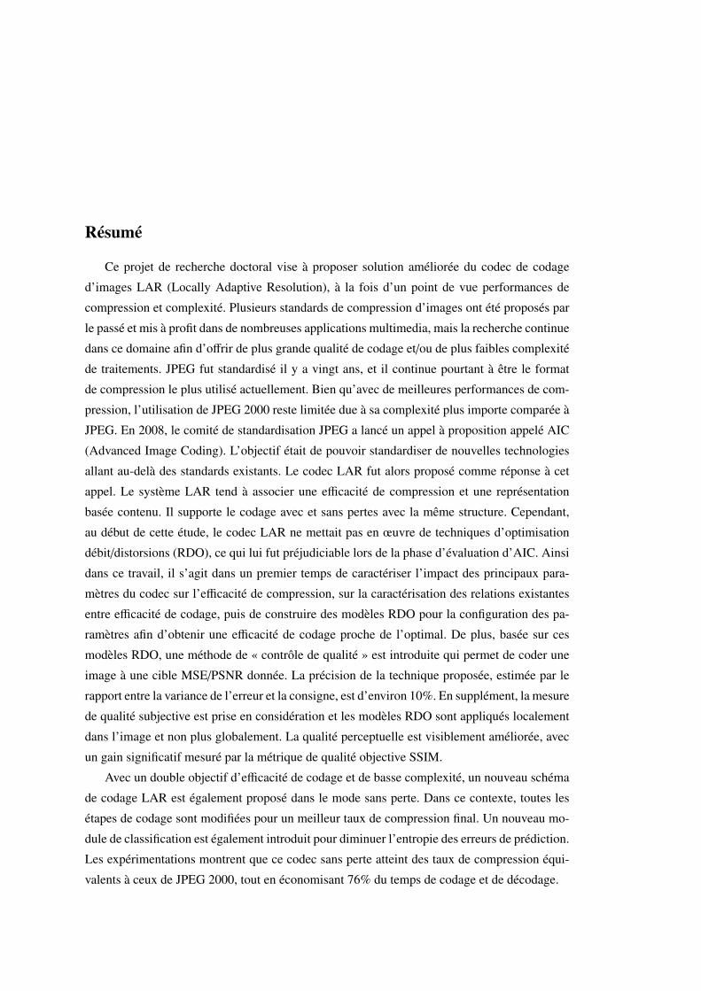
Résumé
Ce projet de recherche doctoral vise à proposer solution améliorée du codec de codage
d’images LAR (Locally Adaptive Resolution), à la fois d’un point de vue performances de
compression et complexité. Plusieurs standards de compression d’images ont été proposés par
le passé et mis à profit dans de nombreuses applications multimedia, mais la recherche continue
dans ce domaine afin d’offrir de plus grande qualité de codage et/ou de plus faibles complexité
de traitements. JPEG fut standardisé il y a vingt ans, et il continue pourtant à être le format
de compression le plus utilisé actuellement. Bien qu’avec de meilleures performances de com-
pression, l’utilisation de JPEG 2000 reste limitée due à sa complexité plus importe comparée à
JPEG. En 2008, le comité de standardisation JPEG a lancé un appel à proposition appelé AIC
(Advanced Image Coding). L’objectif était de pouvoir standardiser de nouvelles technologies
allant au-delà des standards existants. Le codec LAR fut alors proposé comme réponse à cet
appel. Le système LAR tend à associer une efficacité de compression et une représentation
basée contenu. Il supporte le codage avec et sans pertes avec la même structure. Cependant,
au début de cette étude, le codec LAR ne mettait pas en œuvre de techniques d’optimisation
débit/distorsions (RDO), ce qui lui fut préjudiciable lors de la phase d’évaluation d’AIC. Ainsi
dans ce travail, il s’agit dans un premier temps de caractériser l’impact des principaux para-
mètres du codec sur l’efficacité de compression, sur la caractérisation des relations existantes
entre efficacité de codage, puis de construire des modèles RDO pour la configuration des pa-
ramètres afin d’obtenir une efficacité de codage proche de l’optimal. De plus, basée sur ces
modèles RDO, une méthode de « contrôle de qualité » est introduite qui permet de coder une
image à une cible MSE/PSNR donnée. La précision de la technique proposée, estimée par le
rapport entre la variance de l’erreur et la consigne, est d’environ 10%. En supplément, la mesure
de qualité subjective est prise en considération et les modèles RDO sont appliqués localement
dans l’image et non plus globalement. La qualité perceptuelle est visiblement améliorée, avec
un gain significatif mesuré par la métrique de qualité objective SSIM.
Avec un double objectif d’efficacité de codage et de basse complexité, un nouveau schéma
de codage LAR est également proposé dans le mode sans perte. Dans ce contexte, toutes les
étapes de codage sont modifiées pour un meilleur taux de compression final. Un nouveau mo-
dule de classification est également introduit pour diminuer l’entropie des erreurs de prédiction.
Les expérimentations montrent que ce codec sans perte atteint des taux de compression équi-
valents à ceux de JPEG 2000, tout en économisant 76% du temps de codage et de décodage.
Abstract
This doctoral research project aims at designing an improved solution of the still image
codec called LAR (Locally Adaptive Resolution) for both compression performance and com-
plexity. Several image compression standards have been well proposed and used in the multi-
media applications, but the research does not stop the progress for the higher coding quality
and/or lower coding consumption. JPEG was standardized twenty years ago, while it is still a
widely used compression format today. With a better coding efficiency, the application of the
JPEG 2000 is limited by its larger computation cost than the JPEG one. In 2008, the JPEG
Committee announced a Call for Advanced Image Coding (AIC). This call aims to standardize
potential technologies going beyond existing JPEG standards. The LAR codec was proposed
as one response to this call. The LAR framework tends to associate the compression efficiency
and the content-based representation. It supports both lossy and lossless coding under the same
structure. However, at the beginning of this study, the LAR codec did not implement the rate-
distortion-optimization (RDO). This shortage was detrimental for LAR during the AIC eva-
luation step. Thus, in this work, it is first to characterize the impact of the main parameters of
the codec on the compression efficiency, next to construct the RDO models to configure para-
meters of LAR for achieving optimal or sub-optimal coding efficiencies. Further, based on the
RDO models, a “quality constraint” method is introduced to encode the image at a given target
MSE/PSNR. The accuracy of the proposed technique, estimated by the ratio between the error
variance and the set-point, is about 10%. Besides, the subjective quality measurement is taken
into consideration and the RDO models are locally applied in the image rather than globally.
The perceptual quality is improved with a significant gain measured by the objective quality
metric SSIM (structural similarity).
Aiming at a low complexity and efficient image codec, a new coding scheme is also propo-
sed in lossless mode under the LAR framework. In this context, all the coding steps are changed
for a better final compression ratio. A new classification module is also introduced to decrease
the entropy of the prediction errors. Experiments show that this lossless codec achieves the
equivalent compression ratio to JPEG 2000, while saving 76% of the time consumption in
average in encoding and decoding.


Résumé
Ce projet de recherche doctoral vise à proposer solution améliorée du codec de codage d’images LAR (Locally Adaptive Resolution), à la fois d’un point de vue performances de compression et complexité. Plusieurs standards de compression d’images ont été proposés par le passé et mis à profit dans de nombreuses applications multimédia, mais la recherche continue dans ce domaine afin d’offrir de plus grande qualité de codage et/ou de plus faibles complexité de traitements. JPEG fut standardisé il y a vingt ans, et il continue pourtant à être le format de compression le plus utilisé actuellement. Bien qu’avec de meilleures performances de compression, l’utilisation de JPEG 2000 reste limitée due à sa complexité plus importe comparée à JPEG. En 2008, le comité de standardisation JPEG a lancé un appel à proposition appelé AIC (Advanced Image Coding). L’objectif était de pouvoir standardiser de nouvelles technologies allant au-delà des standards existants. Le codec LAR fut alors proposé comme réponse à cet appel. Le système LAR tend à associer une efficacité de compression et une représentation basée contenu. Il supporte le codage avec et sans pertes avec la même structure. Cependant, au début de cette étude, le codec LAR ne mettait pas en œuvre de techniques d’optimisation débit/distorsions (RDO), ce qui lui fut préjudiciable lors de la phase d’évaluation d’AIC. Ainsi dans ce travail, il s’agit dans un premier temps de caractériser l’impact des principaux paramètres du codec sur l’efficacité de compression, sur la caractérisation des relations existantes entre efficacité de codage, puis de construire des modèles RDO pour la configuration des paramètres afin d’obtenir une efficacité de codage proche de l’optimal. De plus, basée sur ces modèles RDO, une méthode de « contrôle de qualité » est introduite qui permet de coder une image à une cible MSE/PSNR donnée. La précision de la technique proposée, estimée par le rapport entre la variance de l’erreur et la consigne, est d’environ 10%. En supplément, la mesure de qualité subjective est prise en considération et les modèles RDO sont appliqués localement dans l’image et non plus globalement. La qualité perceptuelle est visiblement améliorée, avec un gain significatif mesuré par la métrique de qualité objective SSIM. Avec un double objectif d’efficacité de codage et de basse complexité, un nouveau schéma de codage LAR est également proposé dans le mode sans perte. Dans ce contexte, toutes les étapes de codage sont modifiées pour un meilleur taux de compression final. Un nouveau module de classification est également introduit pour diminuer l’entropie des erreurs de prédiction. Les expérimentations montrent que ce codec sans perte atteint des taux de compression équivalents à ceux de JPEG 2000, tout en économisant 76% du temps de codage et de décodage.
N° d’ordre : D15 – 06 / 15ISAR 06
Abstract
This doctoral research project aims at designing an improved solution of the still image codec called LAR (Locally Adaptive Resolution) for both compression performance and complexity. Several image compression standards have been well proposed and used in the multimedia applications, but the research does not stop the progress for the higher coding quality and/or lower coding consumption. JPEG was standardized twenty years ago, while it is still a widely used compression format today. With a better coding efficiency, the application of the JPEG 2000 is limited by its larger computation cost than the JPEG one. In 2008, the JPEG Committee announced a Call for Advanced Image Coding (AIC). This call aims to standardize potential technologies going beyond existing JPEG standards. The LAR codec was proposed as one response to this call. The LAR framework tends to associate the compression efficiency and the content-based representation. It supports both lossy and lossless coding under the same structure. However, at the beginning of this study, the LAR codec did not implement the rate-distortion-optimization (RDO). This shortage was detrimental for LAR during the AIC evaluation step. Thus, in this work, it is first to characterize the impact of the main parameters of the codec on the compression efficiency, next to construct the RDO models to configure parameters of LAR for achieving optimal or sub-optimal coding efficiencies. Further, based on the RDO models, a “quality constraint” method is introduced to encode the image at a given target MSE/PSNR. The accuracy of the proposed technique, estimated by the ratio between the error variance and the set-point, is about 10%. Besides, the subjective quality measurement is taken into consideration and the RDO models are locally applied in the image rather than globally. The perceptual quality is improved with a significant gain measured by the objective quality metric SSIM (structural similarity). Aiming at a low complexity and efficient image codec, a new coding scheme is also proposed in lossless mode under the LAR framework. In this context, all the coding steps are changed for a better final compression ratio. A new classification module is also introduced to decrease the entropy of the prediction errors. Experiments show that this lossless codec achieves the equivalent compression ratio to JPEG 2000, while saving 76% of the time consumption in average in encoding and decoding.
Related Documents