Long-term Population Projections for Massachusetts Regions and Municipalities Prepared for the Office of the Secretary of the Commonwealth of Massachusetts Henry Renski, PhD University of Massachusetts, Amherst Department of Landscape Architecture and Regional Planning Lindsay Koshgarian, M.P.P. Research Manager, Economic and Public Policy Research UMass Donahue Institute Susan Strate Population Estimates Program Manager UMass Donahue Institute November 2013

Welcome message from author
This document is posted to help you gain knowledge. Please leave a comment to let me know what you think about it! Share it to your friends and learn new things together.
Transcript
Long-term Population Projections for
Massachusetts Regions and
Municipalities
Prepared for the Office of the Secretary of the Commonwealth of Massachusetts
Henry Renski, PhD
University of Massachusetts, Amherst
Department of Landscape Architecture and Regional Planning
Lindsay Koshgarian, M.P.P.
Research Manager, Economic and Public Policy Research
UMass Donahue Institute
Susan Strate
Population Estimates Program Manager
UMass Donahue Institute
November 2013
2
Table of Contents
I. Project Overview 6
II. State-Level Summary 8
III. Long Term Regional Population Projections 12
A. Introduction 12
B. Analysis by Region
1. Berkshire/Franklin Region 15
2. Cape and Islands Region 19
3. Central Region 23
4. Greater Boston Region 27
5. Lower Pioneer Valley Region 32
6. MetroWest Region 37
7. Northeast Region 41
8. Southeast Region 45
IV. Technical Discussion of Methods and Assumptions 49
A. Regional-Level Methods and Assumptions 49
Summary 49
Regional definitions 50
Estimating the components of change 51
Determining the launch year and cohort classes 51
Deaths and Survival 51
Domestic Migration 51
International Migration (immigration and emigration) __________53
Births and Fertility 55
Aging the population and generating projections for later years 56
B. Municipal-Level Methods and Assumptions 57
MCD-Level Model Overview 57
Data Sources 57
MCD Projections Launch Population 58
MCD Projections: Mortality 58
MCD Projections: Migration 59
Fertility 60
Controlling to the Regional-level Projections 61
Sources 62
Appendices:
Appendix A: UMDI Population Projections Advisory Committee Members
Appendix B: Detailed Projections by Age, Sex, and Municipality
3
List of Tables and Figures
Figure 2.1: Massachusetts Actual and Projected Population, 2000- 2030 8 Figure 2.2: Actual and Projected Percent Change in Massachusetts Population, 2000-2030 8 Figure 2.3: Massachusetts Actual and Projected Population by Cohort, 2010, 2020, and 2030 9 Figure 2.4: Massachusetts Projected Population Distribution by Age Group, 2010-2030 10 Figure 2.5: Actual and Projected Percentage Growth by 10-Year Period for Massachusetts, the United States, and the Northeast Region 1990-2030 10 Figure 2.6: Projected Percentage Growth by Massachusetts Region, 2010-2030 _________ 11 Figure 3.1: Massachusetts Regions for Population Forecasts 12 Figure 3.1a: The Berkshire/Franklin Region 15
Figure 3.1b: Recent and projected population, Berkshire/Franklin 15 Figure 3.1c: Annualized rates of population change, Berkshire/Franklin 15 Table 3.1: Summary Results, Estimated Components of Population Change, Berkshire/Franklin 16 Figure 3.1d: Age profile of net domestic migrants, 2005 to 2010, Berkshire/Franklin 16 Figure 3.1e: Projected levels of domestic in and out-migration, 2005 to 2030, Berkshire/Franklin 17 Figure 3.1f: Projected levels of births and deaths, 2005 to 2030, Berkshire/Franklin 17 Figure 3.1g: The age and gender composition of the Berkshire/Franklin population, 2010 (actual) vs. 2030 (forecasted) 18 Figure 3.2a: The Cape and Islands Region 19
Figure 3.2b: Recent and projected population, Cape and Islands 19 Figure 3.2c: Annualized rates of population change, Cape and Islands _ 19 Table 3.2: Summary Results, Estimated Components of Population Change, Cape and Islands 20 Figure 3.2d: Age profile of net domestic migrants, 2005 to 2010, Cape and Islands 20 Figure 3.2e: Projected levels of domestic in and out-migration, 2005 to 2030, Cape and Islands 21 Figure 3.2f: Projected levels of births and deaths, 2005 to 2030, Cape and Islands 21 Figure 3.2g: The age and gender composition of the Cape and Islands population, 2010 (actual) vs. 2030 (forecasted) 22 Figure 3.3a: The Central Region 23 Figure 3.3b: Recent and projected population, Central Region 23
4
Figure 3.3c: Annualized rates of population change, Central Region 23 Table 3.3: Summary Results, Estimated Components of Population Change, Central Region 24
Figure 3.3d: Age profile of net domestic migrants, 2005 to 2010, Central Region 24 Figure 3.3e: Projected levels of domestic in and out-migration, 2005 to 2030, Central Region 25 Figure 3.3f: Projected levels of births and deaths, 2005 to 2030, Central Region 25 Figure 3.3g: The age and gender composition of the Central region population, 2010 (actual) vs. 2030 (forecasted) 26 Figure 3.4a: The Greater Boston Region 27 Figure 3.4b: Projected Population, Greater Boston 27 Figure 3.4c: Annualized rates of population change, Greater Boston 27 Table 3.4: Summary Results, Estimated Components of Population Change, Greater Boston 28 Figure 3.4d: Age profile of net domestic migrants, 2005 to 2010, Greater Boston 28 Figure 3.4e: Projected levels of domestic in and out-migration, 2005 to 2030, Greater Boston 30 Figure 3.4f: Projected levels of births and deaths, 2005 to 2030, Greater Boston 30 Figure 3.4g: The age and gender composition of the Greater Boston region, 2010 (actual) vs. 2030 (forecasted) 31 Figure 3.5a: The Lower Pioneer Valley Region 32 Figure 3.5b: Projected Population, Lower Pioneer Valley 32 Figure 3.5c: Annualized rates of population change, Lower Pioneer Valley 32 Table 3.5: Summary Results, Estimated Components of Population Change, Lower Pioneer Valley 33 Figure 3.5d: Age profile of net domestic migrants, 2005 to 2010, Lower Pioneer Valley 33 Figure 3.5e: Projected levels of domestic in and out-migration, 2005 to 2030, Lower Pioneer Valley 34 Figure 3.5f: Projected levels of births and deaths, 2005 to 2030, Lower Pioneer Valley 34 Figure 3.5g: The age and gender composition of the Lower Pioneer Valley, 2010 (actual) vs. 2030 (forecasted) 35 Figure 3.6a: The MetroWest Region 37 Figure 3.6b: Projected Population, MetroWest 37
5
Figure 3.6c: Annualized rates of population change, MetroWest 37 Table 3.6: Summary Results, Estimated Components of Population Change, MetroWest 38 Figure 3.6d: Age profile of net domestic migrants, 2005 to 2010, MetroWest 38 Figure 3.6e: Projected levels of domestic in and out-migration, 2005 to 2030, MetroWest 39 Figure 3.6f: Projected levels of births and deaths, 2005 to 2030, MetroWest 39 Figure 3.6g: The age and gender composition of the MetroWest Region, 2010 (actual) vs. 2030 (forecasted) 40 Figure 3.7a: The Northeast Region 41 Figure 3.7b: Projected Population, Northeast Region 41 Figure 3.7c: Annualized rates of population change, Northeast Region 41 Table 3.7: Summary Results, Estimated Components of Population Change, Northeast Region 42 Figure 3.7d: Age profile of net domestic migrants, 2005 to 2010, Northeast Region 42 Figure 3.7e: Projected levels of domestic in and out-migration, 2005 to 2030, Northeast Region 43 Figure 3.7f: Projected levels of births and deaths, 2005 to 2030, Northeast Region 43 Figure 3.7g: The age and gender composition of the Northeast Region, 2010 (actual) vs. 2030 (forecasted) 44 Figure 3.8a: The Southeast Region 45 Figure 3.8b: Projected Population, Southeast Region 45 Figure 3.8c: Annualized rates of population change, Southeast Region 45 Table 3.8: Summary Results, Estimated Components of Population Change, Southeast Region 46 Figure 3.8d: Age profile of net domestic migrants, 2005 to 2010, Southeast Region 46 Figure 3.8e: Projected levels of domestic in and out-migration, 2005 to 2030, Southeast Region 47 Figure 3.8f: Projected levels of births and deaths, 2005 to 2030, Southeast Region 47 Figure 3.8g: The age and gender composition of the Southeast Region, 2010 (actual) vs. 2030 (forecasted) 48 Figure 4.1: Massachusetts Regions for Population Forecasts 50
6
I. Project Overview
Massachusetts agencies and entities have not had access to detailed, publically available, statewide
municipal population projections by age and sex since the Massachusetts Institute for Social and
Economic Research (MISER) last produced projections in 2003 based on Census 2000. The U.S.
Census Bureau previously produced state-level projections by age and sex, but has at present
discontinued them, with the last Census-produced state population projections based on Census
2000 data and released in 2005. These projections do not reflect the shift in economic and social
trends that has taken place since 2000, and their usefulness has likely passed. While some regional
planning agencies (RPAs) and statewide agencies produce municipal population projections, they
are limited to either municipal totals, subsets of the population (i.e. children of school age), or
certain geographical regions, and their methodologies vary. Agencies with broad, statewide
planning needs such as water resource management or public health are challenged with having to
somehow reconcile different and sometimes conflicting sets of methods and results, when
municipal projections are available at all.
Massachusetts is also in a minority of states that do not produce regularly updated population
projections. According to a 2009 member survey by the Federal State Cooperative for Population
Projections (FSCPP; a partnership between the U.S. Census Bureau and designated state agencies),
only eight states – including Massachusetts – do not regularly produce publicly available population
projections. Thirty-nine states produce at least state and county level projections; 35 produce these
at least every two years.
To meet this statewide need, the Massachusetts Secretary of the Commonwealth contracted with
the University of Massachusetts Donahue Institute (UMDI) to produce population projections by
age and sex for all 351 municipalities (also referred to here as minor civil divisions – or MCDs) in
Massachusetts.
The resulting set is the product of well over a year of preparation and analysis by experienced
researchers on the UMDI staff as well as input and commentary by an Advisory Committee that
included public stakeholders as well as state and national experts working in the field.1 The
methodology was developed by Dr. Henry Renski of the University of Massachusetts in Amherst,
who previously produced projections for the state of Maine and who is well regarded and published
in the fields of regional planning and projections methods.
UMDI produced cohort component model projections for two different geographic levels:
municipalities and eight sub-state regions that we defined for this purpose. These sub-state regions
include the Berkshire/Franklin, Cape and Islands, Central, Greater Boston, Lower Pioneer Valley,
MetroWest, Northeast, and Southeast regions. The UMDI projections are available for all
1 Listed in Appendix A: UMDI Population Projections Advisory Committee Members
7
municipalities by sex and 5-year age groups, from 0-4 through 85+, and at 5-year intervals
beginning in 2015 and ending in 2030. While the municipal-level projections provide a great level
of detail, the regional projections describe in broad strokes the ways that components of change
such as fertility, mortality, and migration are expected to play out over the next few decades in each
part of the state, according to our projections model.
Modeled projections cannot and do not purport to predict the future, but rather may serve as points
of reference for planners and researchers. Like all forecasts, the UMDI projections rely upon
assumptions about future trends based on past and present trends which may or may not actually
persist into the future. In general, projections for small geographies and distant futures will be less
predictive than projections for larger populations and near terms. Also, any statewide method will
tend to produce unusual looking results in very small geographies or in small age cohorts. While
our method makes adjustments for small geographies or cohorts in some of its rates, researchers
are nonetheless encouraged to use their best judgment in deciding for which cases aggregate
populations are more appropriately used.
For our projections, we use a cohort-component model based on trends in fertility, mortality, and
migration from 2000 through 2011. Our regional-level method makes use of American Community
Survey sample data on migration rates by age and uses a gross, multi-regional approach in
forecasting future levels of migration. Our sub-regional, municipal-level estimates rely instead on
residual net migration rates computed from vital statistics. The municipal-level method is applied
uniformly to all municipalities in Massachusetts, except for adjustments made to calculated rates in
very small geographies. The municipal projections are finally controlled to the regional projections
to produce the end results.
The next section of this report, Section II. State-Level Summary, highlights the total population
change anticipated for Massachusetts through 2030 after the regional projections are summed
together, while the subsequent Section III describes in greater detail the regional-level population
projections, including an Analysis section for each of the eight distinct Massachusetts regions.
Section IV of this report, Technical Discussion of Methods and Assumptions, provides more specific
information on both the regional and MCD-level projections methods utilized here, and finally
attached are the MDC-level projection results to 2030.
8
2000-2005
2005-2010
2010-2015
2015-2020
2020-2025
2025-2030
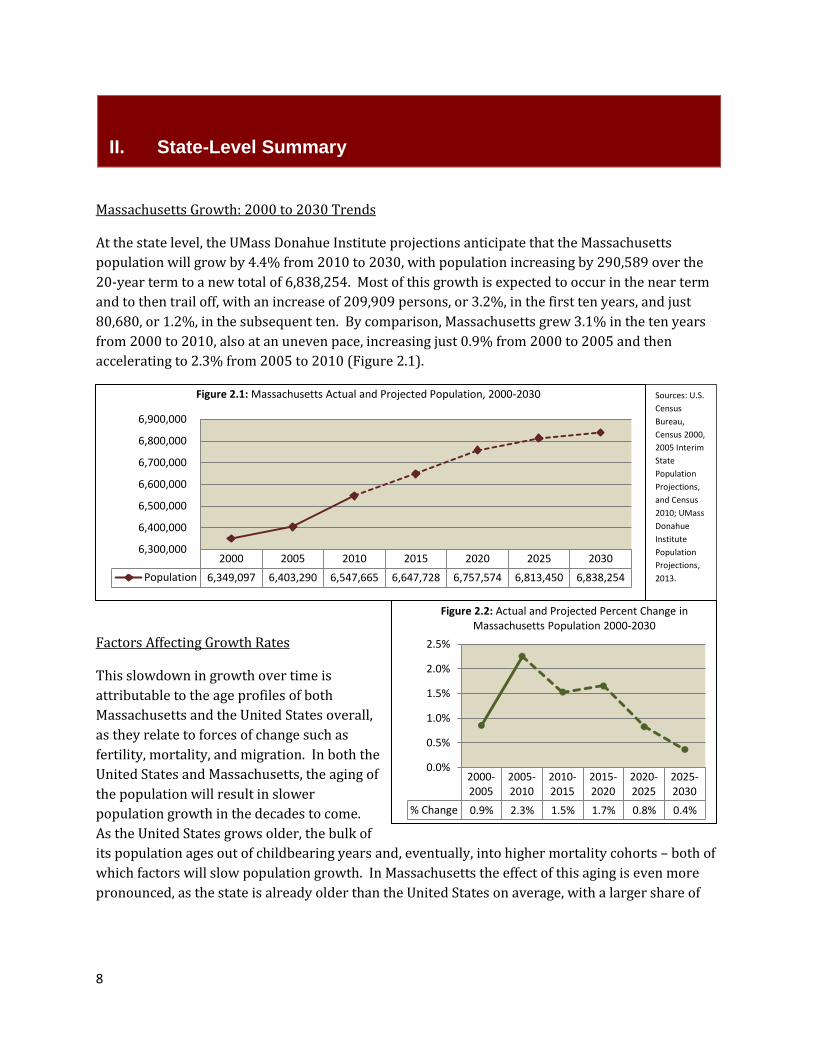
% Change 0.9% 2.3% 1.5% 1.7% 0.8% 0.4%
0.0%
0.5%
1.0%
1.5%
2.0%
2.5%
Figure 2.2: Actual and Projected Percent Change in Massachusetts Population 2000-2030
Sources: U.S.
Census
Bureau,
Census 2000,
2005 Interim
State
Population
Projections,
and Census
2010; UMass
Donahue
Institute
Population
Projections,
2013.
2000 2005 2010 2015 2020 2025 2030
Population 6,349,097 6,403,290 6,547,665 6,647,728 6,757,574 6,813,450 6,838,254
6,300,000
6,400,000
6,500,000
6,600,000
6,700,000
6,800,000
6,900,000
Figure 2.1: Massachusetts Actual and Projected Population, 2000-2030
II. State-Level Summary
Massachusetts Growth: 2000 to 2030 Trends
At the state level, the UMass Donahue Institute projections anticipate that the Massachusetts
population will grow by 4.4% from 2010 to 2030, with population increasing by 290,589 over the
20-year term to a new total of 6,838,254. Most of this growth is expected to occur in the near term
and to then trail off, with an increase of 209,909 persons, or 3.2%, in the first ten years, and just
80,680, or 1.2%, in the subsequent ten. By comparison, Massachusetts grew 3.1% in the ten years
from 2000 to 2010, also at an uneven pace, increasing just 0.9% from 2000 to 2005 and then
accelerating to 2.3% from 2005 to 2010 (Figure 2.1).
Factors Affecting Growth Rates
This slowdown in growth over time is
attributable to the age profiles of both
Massachusetts and the United States overall,
as they relate to forces of change such as
fertility, mortality, and migration. In both the
United States and Massachusetts, the aging of
the population will result in slower
population growth in the decades to come.
As the United States grows older, the bulk of
its population ages out of childbearing years and, eventually, into higher mortality cohorts – both of
which factors will slow population growth. In Massachusetts the effect of this aging is even more
pronounced, as the state is already older than the United States on average, with a larger share of
9
population in the older age-groups and a smaller share in the younger2. An increasing pool of
retirees in Massachusetts exacerbates this effect to some extent by increasing out-migration from
many regions of the state to places in the South and West, while a group of younger, post-college
cohorts also continues to contribute to a net domestic outflow.
While an aging population means slowed population growth in Massachusetts from 2010 to 2030,
the slowdown is somewhat tempered in the first 10 years, in part by a large “millennial” generation
in the United States overall. This group is now aging into the cohorts associated with increased
migration to college and work destinations, factors that historically have led to population increase
in Massachusetts, especially in the Greater Boston region. At the top end, this generation is also
entering the age group associated with starting families, and so additionally increases the overall
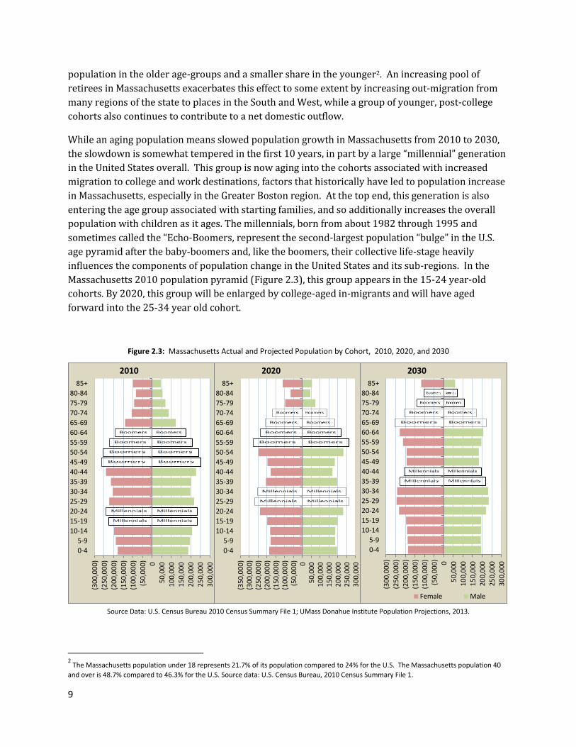
population with children as it ages. The millennials, born from about 1982 through 1995 and
sometimes called the “Echo-Boomers, represent the second-largest population “bulge” in the U.S.
age pyramid after the baby-boomers and, like the boomers, their collective life-stage heavily
influences the components of population change in the United States and its sub-regions. In the
Massachusetts 2010 population pyramid (Figure 2.3), this group appears in the 15-24 year-old
cohorts. By 2020, this group will be enlarged by college-aged in-migrants and will have aged
forward into the 25-34 year old cohort.
Figure 2.3: Massachusetts Actual and Projected Population by Cohort, 2010, 2020, and 2030
Source Data: U.S. Census Bureau 2010 Census Summary File 1; UMass Donahue Institute Population Projections, 2013.
2 The Massachusetts population under 18 represents 21.7% of its population compared to 24% for the U.S. The Massachusetts population 40
and over is 48.7% compared to 46.3% for the U.S. Source data: U.S. Census Bureau, 2010 Census Summary File 1.
(30
0,0
00
)
(25
0,0
00
)
(20
0,0
00
)
(15
0,0
00
)
(10
0,0
00
)
(50
,00
0) 0
50
,00
0
10
0,0
00
15
0,0
00
20
0,0
00
25
0,0
00
30
0,0
00
0-4
5-9
10-14
15-19
20-24
25-29
30-34
35-39
40-44
45-49
50-54
55-59
60-64
65-69
70-74
75-79
80-84
85+
2010
(35
0,0
00
)(3
00
,00
0)
(25
0,0
00
)(2
00
,00
0)
(15
0,0
00
)(1
00
,00
0)
(50
,00
0) 0
50
,00
01
00,
00
01
50,
00
02
00,
00
02
50,
00
03
00,
00
0
0-4
5-9
10-14
15-19
20-24
25-29
30-34
35-39
40-44
45-49
50-54
55-59
60-64
65-69
70-74
75-79
80-84
85+
2020
(30
0,0
00
)
(25
0,0
00
)
(20
0,0
00
)
(15
0,0
00
)
(10
0,0
00
)
(50
,00
0) 0
50
,00
0
10
0,0
00
15
0,0
00
20
0,0
00
25
0,0
00
30
0,0
00
0-4
5-9
10-14
15-19
20-24
25-29
30-34
35-39
40-44
45-49
50-54
55-59
60-64
65-69
70-74
75-79
80-84
85+
2030
Female Male
10
0.00%
2.00%
4.00%
6.00%
8.00%
10.00%
12.00%
14.00%
1990-2000 2000-2010 2010-2020 2020-2030
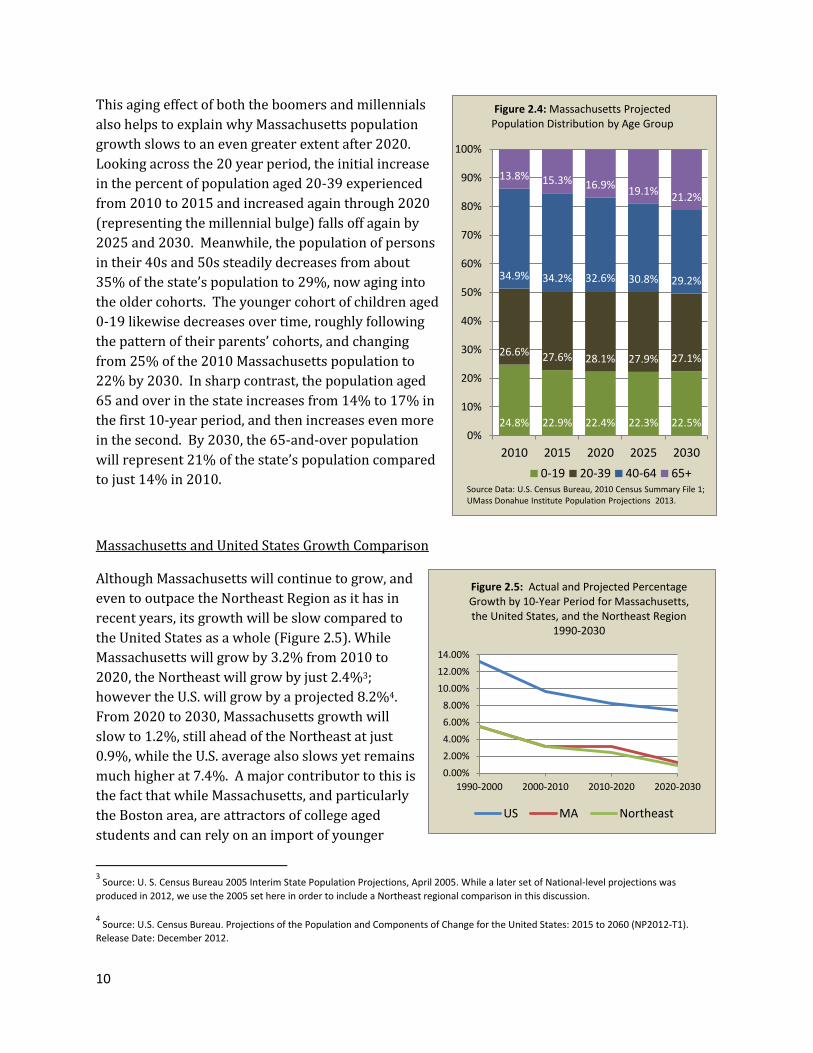
Figure 2.5: Actual and Projected Percentage Growth by 10-Year Period for Massachusetts, the United States, and the Northeast Region
1990-2030
US MA Northeast
24.8% 22.9% 22.4% 22.3% 22.5%
26.6% 27.6% 28.1% 27.9% 27.1%
34.9% 34.2% 32.6% 30.8% 29.2%
13.8% 15.3% 16.9% 19.1%
21.2%
0%
10%
20%
30%
40%
50%
60%
70%
80%
90%
100%
2010 2015 2020 2025 2030
Figure 2.4: Massachusetts Projected Population Distribution by Age Group
0-19 20-39 40-64 65+Source Data: U.S. Census Bureau, 2010 Census Summary File 1; UMass Donahue Institute Population Projections 2013.
This aging effect of both the boomers and millennials
also helps to explain why Massachusetts population
growth slows to an even greater extent after 2020.
Looking across the 20 year period, the initial increase
in the percent of population aged 20-39 experienced
from 2010 to 2015 and increased again through 2020
(representing the millennial bulge) falls off again by
2025 and 2030. Meanwhile, the population of persons
in their 40s and 50s steadily decreases from about
35% of the state’s population to 29%, now aging into
the older cohorts. The younger cohort of children aged
0-19 likewise decreases over time, roughly following
the pattern of their parents’ cohorts, and changing
from 25% of the 2010 Massachusetts population to
22% by 2030. In sharp contrast, the population aged
65 and over in the state increases from 14% to 17% in
the first 10-year period, and then increases even more
in the second. By 2030, the 65-and-over population
will represent 21% of the state’s population compared
to just 14% in 2010.
Massachusetts and United States Growth Comparison
Although Massachusetts will continue to grow, and
even to outpace the Northeast Region as it has in
recent years, its growth will be slow compared to
the United States as a whole (Figure 2.5). While
Massachusetts will grow by 3.2% from 2010 to
2020, the Northeast will grow by just 2.4%3;
however the U.S. will grow by a projected 8.2%4.
From 2020 to 2030, Massachusetts growth will
slow to 1.2%, still ahead of the Northeast at just
0.9%, while the U.S. average also slows yet remains
much higher at 7.4%. A major contributor to this is
the fact that while Massachusetts, and particularly
the Boston area, are attractors of college aged
students and can rely on an import of younger
3 Source: U. S. Census Bureau 2005 Interim State Population Projections, April 2005. While a later set of National-level projections was
produced in 2012, we use the 2005 set here in order to include a Northeast regional comparison in this discussion. 4 Source: U.S. Census Bureau. Projections of the Population and Components of Change for the United States: 2015 to 2060 (NP2012-T1).
Release Date: December 2012.
11
people into the state, other parts of the United States start out with much higher percentages of
younger cohorts already resident in their age profiles, especially in the 0-18 year old age groups5.
Lagging behind U.S. growth is also not new for Massachusetts. From 1990 to 2000 the U.S grew
13.2% compared to 5.5% for Massachusetts and the Northeast region. Similarly, from 2000 to 2010
the U.S. grew by 9.7% compared to 3.2% in the Northeast and 3.1% in Massachusetts6.
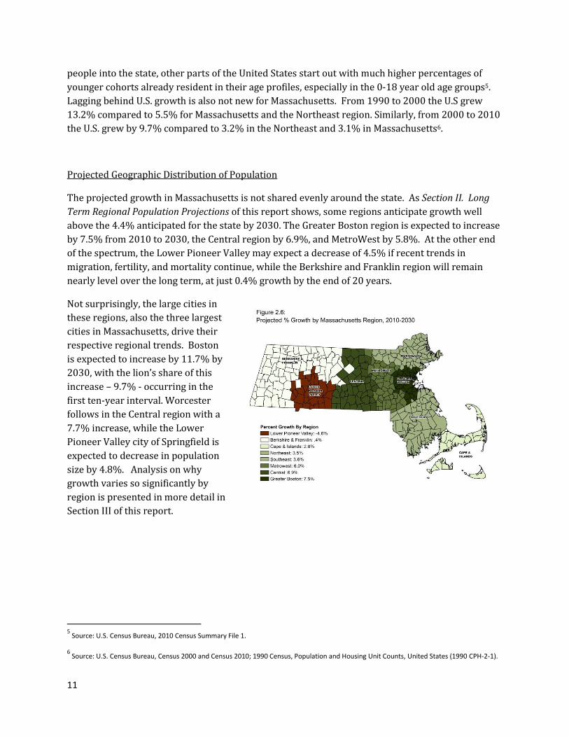
Projected Geographic Distribution of Population
The projected growth in Massachusetts is not shared evenly around the state. As Section II. Long
Term Regional Population Projections of this report shows, some regions anticipate growth well
above the 4.4% anticipated for the state by 2030. The Greater Boston region is expected to increase
by 7.5% from 2010 to 2030, the Central region by 6.9%, and MetroWest by 5.8%. At the other end
of the spectrum, the Lower Pioneer Valley may expect a decrease of 4.5% if recent trends in
migration, fertility, and mortality continue, while the Berkshire and Franklin region will remain
nearly level over the long term, at just 0.4% growth by the end of 20 years.
Not surprisingly, the large cities in
these regions, also the three largest
cities in Massachusetts, drive their
respective regional trends. Boston
is expected to increase by 11.7% by
2030, with the lion’s share of this
increase – 9.7% - occurring in the
first ten-year interval. Worcester
follows in the Central region with a
7.7% increase, while the Lower
Pioneer Valley city of Springfield is
expected to decrease in population
size by 4.8%. Analysis on why
growth varies so significantly by
region is presented in more detail in
Section III of this report.
5 Source: U.S. Census Bureau, 2010 Census Summary File 1.
6 Source: U.S. Census Bureau, Census 2000 and Census 2010; 1990 Census, Population and Housing Unit Counts, United States (1990 CPH-2-1).
12
III. Long Term Regional Population Projections
A. Introduction
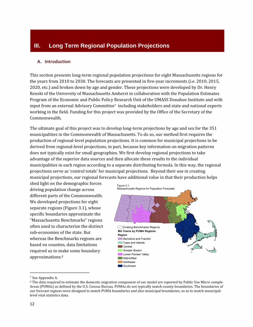
This section presents long-term regional population projections for eight Massachusetts regions for
the years from 2010 to 2030. The forecasts are presented in five-year increments (i.e. 2010, 2015,
2020, etc.) and broken down by age and gender. These projections were developed by Dr. Henry
Renski of the University of Massachusetts Amherst in collaboration with the Population Estimates
Program of the Economic and Public Policy Research Unit of the UMASS Donahue Institute and with
input from an external Advisory Committee7 including stakeholders and state and national experts
working in the field. Funding for this project was provided by the Office of the Secretary of the
Commonwealth.
The ultimate goal of this project was to develop long-term projections by age and sex for the 351
municipalities in the Commonwealth of Massachusetts. To do so, our method first requires the
production of regional-level population projections. It is common for municipal projections to be
derived from regional-level projections, in part, because key information on migration patterns
does not typically exist for small geographies. We first develop regional projections to take
advantage of the superior data sources and then allocate these results to the individual
municipalities in each region according to a separate distributing formula. In this way, the regional
projections serve as ‘control totals’ for municipal projections. Beyond their use in creating
municipal projections, our regional forecasts have additional value in that their production helps
shed light on the demographic forces
driving population change across
different parts of the Commonwealth.
We developed projections for eight
separate regions (Figure 3.1), whose
specific boundaries approximate the
“Massachusetts Benchmarks” regions
often used to characterize the distinct
sub-economies of the state. But
whereas the Benchmarks regions are
based on counties, data limitations
required us to make some boundary
approximations.8
7 See Appendix A. 8 The data required to estimate the domestic migration component of our model are reported by Public Use Micro-sample Areas (PUMAs) as defined by the U.S. Census Bureau. PUMAs do not typically match county boundaries. The boundaries of our forecast regions were designed to match PUMA boundaries and also municipal boundaries, so as to match municipal-level vital statistics data.
13
Our projections are based on a demographic accounting framework for modeling population
change, commonly referred to as a cohort-component model.9 The cohort-component approach
recognizes only four ways by which a regions population can change from one time period to the
next. It can add residents through either births or in-migration, and it can lose residents through
deaths or out-migration.
The cohort-component model also accounts for regional difference in the age profile of its residents.
Birth, death, in- and out-migration rates all vary by age and across regions. To account for this, a
cohort-component model classifies the regional population into five year age “cohorts” (e.g. 0 to 4
years old, 5 to 9,… 80 to 84, and 85 or older) and develops separate profiles for males and females.
We use data from the recent past (primarily 2005 to 2010) to determine the contribution of each
component to the changes in the population within each age-sex cohort. The counts are converted
into rates by dividing each by the appropriate eligible population. We then apply these rates to the
applicable cohort population in the forecast launch year (for us, 2010) in order to measure the
anticipated number of births, deaths, and migrants in the next five years. The number of anticipated
births, deaths and migrants are added to the launch year population in order to predict the cohort
population five years into the future. As a final step, the surviving resident population of each
cohort is aged by five years, and becomes the baseline for the next iteration of projections.
Our approach to cohort-component modeling in this projections set introduces several
methodological innovations not found in the standard practice of cohort-component modeling.
Most follow a net-migration approach, where a single net migration rate is calculated as the number
of net new migrants (in-migrants minus out-migrants) divided by the baseline population of the
study region. While commonly used, this approach has been shown to lead to erroneous
projections—particularly for fast growing and declining regions (Isserman 1993). Instead, we use a
gross-migration approach that develops separate rates for domestic in- and out-migrants. The
candidate pool of in-migration is based on people not currently living in the region, thereby tying
regional population change to broader regional and national forces.10 We further divide domestic
in-migrants into those originating in from neighboring regions and states and those coming from
elsewhere in the U.S. to further improve the accuracy of our estimates. This type of model is made
possible by utilizing the rich detail of information available through the newly released Public Use
Micro-Samples of American Community Survey. We also include a residual component, which
accounts for unknown measurement and sampling error in the data and prevents the model from
departing too dramatically from historical trends.
While we take pride in using highly detailed data and a state of the art modeling approach, no one
can predict the future with certainty. Our projections are simply one possible scenario of the
future—one conditioned largely on whether recent trends in births, deaths and migration continue
into the foreseeable future. If past trends continue, then we believe that our model should provide
an accurate reflection of population change. However, past trends rarely continue. Economic
expansion and recessionary cycles, medical and technological breakthroughs, changes in cultural 9 A more detailed description of our methodology is provided in Section IV. of this report: Technical Discussion of Methods and Assumptions. 10 The rationale behind the development of a distinct in-migration rate is that the potential population of in-migrants is not the people already living in the region (as assumed in a net migration approach), but those living anywhere but.

14
norms and lifestyle preferences, regional differences in climate change, even state and federal
policies – all of the above and more can and will influence birth, death and migration behavior. We
humbly admit that we lack the clairvoyance to predict what these changes will be in the next two
decades and what they will mean for Massachusetts and its residents. Of particular note is the
consideration that the data used for developing component-specific rates of change were largely
collected for the years of 2005 to 2010. This period covers, in equal parts, periods of relative
economic stability and severe recession. It is difficult to say, for example, whether the gradual
economic recovery will lead to an upswing in births following a period where many families put-off
having children, or whether birth rates will rebound slightly and thus return to the longer-term
trend of smaller families. We expect economic recovery to lead to greater mobility, however, we do
not know if this will result in relatively more people moving in our out of Massachusetts. Likewise,
we cannot predict the resolution of contemporary debates over immigration reform, housing policy,
and/or financing of higher education and student loan programs. Nor can we even begin to assess
whether climate change will lead to a re-colonization of the Northeast, which has been steadily
losing population to the South and Southwest for the past several decades. Making predictions like
these is far beyond our collective expertise and the scope of this study.
These caveats are not meant to completely dismiss the validity of our projections, but rather to
situate them in a reasonable context. Population change tends to be a gradual process for most
regions in the Northeast. Most of the people living in a region five years from now will be the same
folks living here today – only a little bit older. Regions with an older resident population can expect
to experience more deaths as these people age. Places with large number of residents in their late
twenties and thirties can expect more births in the coming years. A large number of U.S .residents in
grade school today will mean a larger pool of potential college students ten or fifteen years down
the road. These are many trends that we can anticipate with relative certainty, and which are
reflected in the regional results that follow.
15
B. Analysis by Region
1. Berkshire/Franklin Region
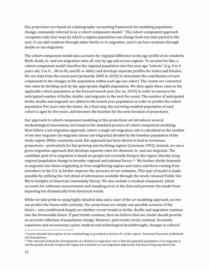
The Berkshire/Franklin county region
consists of 76 communities spanning the
Commonwealth’s western and northwestern
borders. It is predominantly rural, with its
primary population and employment centers
of Pittsfield in Berkshire County and
Greenfield in Franklin County.
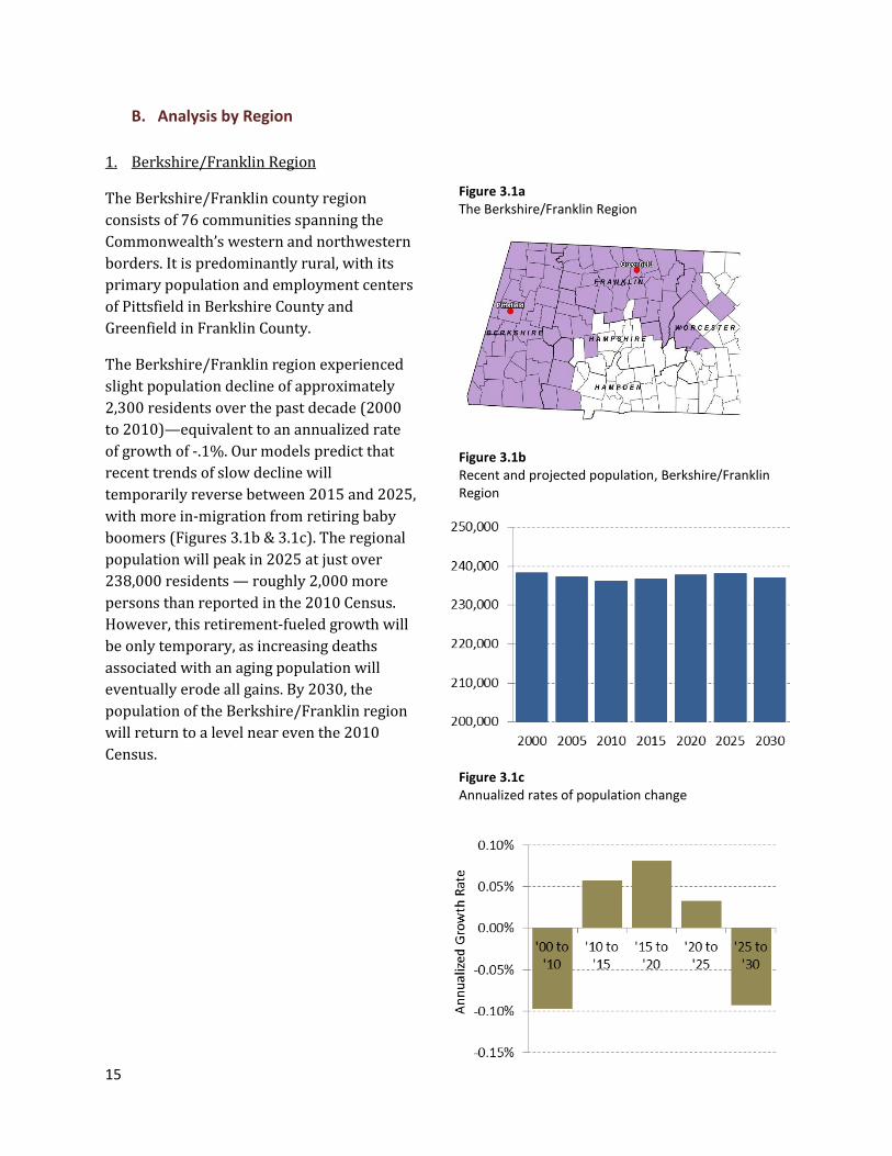
The Berkshire/Franklin region experienced
slight population decline of approximately
2,300 residents over the past decade (2000
to 2010)—equivalent to an annualized rate
of growth of -.1%. Our models predict that
recent trends of slow decline will
temporarily reverse between 2015 and 2025,
with more in-migration from retiring baby
boomers (Figures 3.1b & 3.1c). The regional
population will peak in 2025 at just over
238,000 residents — roughly 2,000 more
persons than reported in the 2010 Census.
However, this retirement-fueled growth will
be only temporary, as increasing deaths
associated with an aging population will
eventually erode all gains. By 2030, the
population of the Berkshire/Franklin region
will return to a level near even the 2010
Census.
Figure 3.1b Recent and projected population, Berkshire/Franklin Region
Figure 3.1c Annualized rates of population change
Figure 3.1a The Berkshire/Franklin Region
16
The Sources of Population Change
Table 3.1 Summary Results: Estimated Components of Population Change, Berkshire/Franklin Region
2005 to
2010 2010 to
2015 2015 to
2020 2020 to
2025 2025 to
2030
Starting Population 237,222 236,058 236,728 237,689 238,078
Births 10,833 10,526 9,644 9,364 9,131
Deaths 11,513 12,844 13,798 14,753 16,031
Natural Increase -680 -2,318 -4,154 -5,389 -6,900
Domestic In-migration, MA & Border 33,955 34,169 34,770 34,766 34,935
Domestic In-migration, Rest of U.S. 13,245 13,492 13,990 14,432 14,888
Domestic Out-migration 54,040 52,557 49,939 48,025 47,285
Net Domestic -6,840 -4,896 -1,179 1,173 2,538
Residual (Actual - Predicted Ending Pop.) 6,356 7,884 6,294 4,605 3,254
Ending Population 236,058 236,728 237,689 238,078 236,970
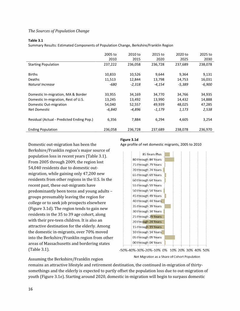
Domestic out-migration has been the
Berkshire/Franklin region’s major source of
population loss in recent years (Table 3.1).
From 2005 through 2009, the region lost
54,040 residents due to domestic out-
migration, while gaining only 47,200 new
residents from other regions in the U.S. In the
recent past, these out-migrants have
predominantly been teens and young adults –
groups presumably leaving the region for
college or to seek job prospects elsewhere
(Figure 3.1d). The region tends to gain new
residents in the 35 to 39 age cohort, along
with their pre-teen children. It is also an
attractive destination for the elderly. Among
the domestic in-migrants, over 70% moved
into the Berkshire/Franklin region from other
areas of Massachusetts and bordering states
(Table 3.1).
Assuming the Berkshire/Franklin region
remains an attractive lifestyle and retirement destination, the continued in-migration of thirty-
somethings and the elderly is expected to partly offset the population loss due to out-migration of
youth (Figure 3.1e). Starting around 2020, domestic in-migration will begin to surpass domestic
Figure 3.1d Age profile of net domestic migrants, 2005 to 2010
17
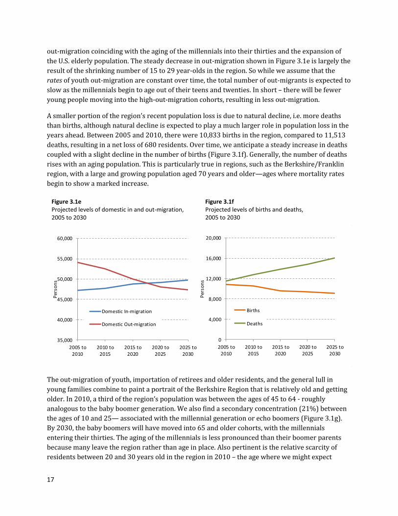
out-migration coinciding with the aging of the millennials into their thirties and the expansion of
the U.S. elderly population. The steady decrease in out-migration shown in Figure 3.1e is largely the
result of the shrinking number of 15 to 29 year-olds in the region. So while we assume that the
rates of youth out-migration are constant over time, the total number of out-migrants is expected to
slow as the millennials begin to age out of their teens and twenties. In short – there will be fewer
young people moving into the high-out-migration cohorts, resulting in less out-migration.
A smaller portion of the region’s recent population loss is due to natural decline, i.e. more deaths
than births, although natural decline is expected to play a much larger role in population loss in the
years ahead. Between 2005 and 2010, there were 10,833 births in the region, compared to 11,513
deaths, resulting in a net loss of 680 residents. Over time, we anticipate a steady increase in deaths
coupled with a slight decline in the number of births (Figure 3.1f). Generally, the number of deaths
rises with an aging population. This is particularly true in regions, such as the Berkshire/Franklin
region, with a large and growing population aged 70 years and older—ages where mortality rates
begin to show a marked increase.
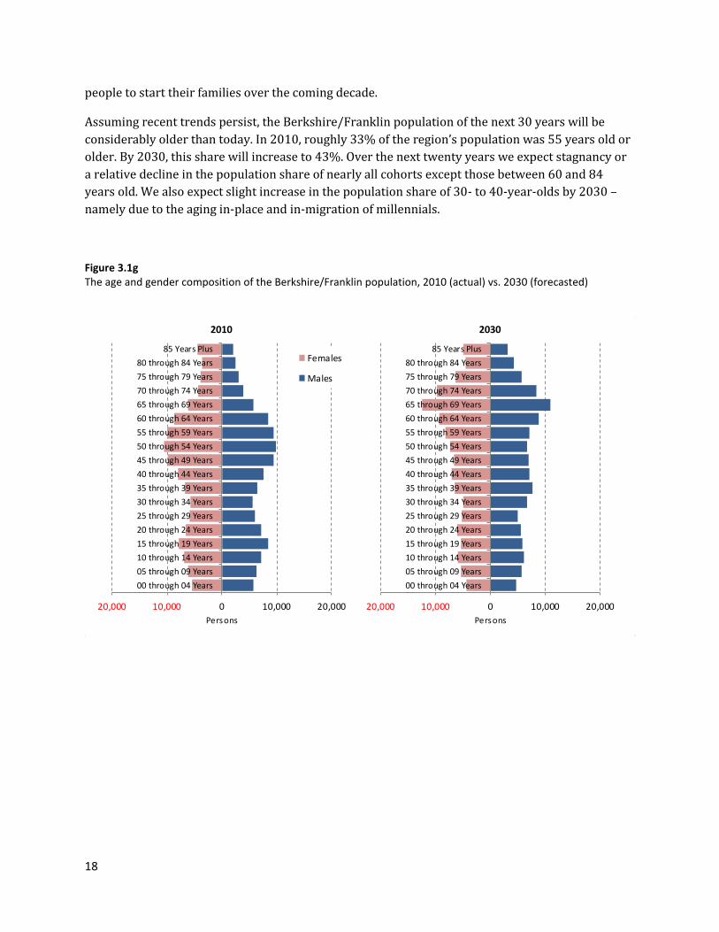
The out-migration of youth, importation of retirees and older residents, and the general lull in
young families combine to paint a portrait of the Berkshire Region that is relatively old and getting
older. In 2010, a third of the region’s population was between the ages of 45 to 64 - roughly
analogous to the baby boomer generation. We also find a secondary concentration (21%) between
the ages of 10 and 25— associated with the millennial generation or echo boomers (Figure 3.1g).
By 2030, the baby boomers will have moved into 65 and older cohorts, with the millennials
entering their thirties. The aging of the millennials is less pronounced than their boomer parents
because many leave the region rather than age in place. Also pertinent is the relative scarcity of
residents between 20 and 30 years old in the region in 2010 – the age where we might expect
35,000
40,000
45,000
50,000
55,000
60,000
2005 to2010
2010 to2015
2015 to2020
2020 to2025
2025 to2030
Per
son
s
Domestic In-migration
Domestic Out-migration
0
4,000
8,000
12,000
16,000
20,000
2005 to2010
2010 to2015
2015 to2020
2020 to2025
2025 to2030
Per
son
s
Births
Deaths
Figure 3.1e Projected levels of domestic in and out-migration, 2005 to 2030
Figure 3.1f Projected levels of births and deaths, 2005 to 2030
18
people to start their families over the coming decade.
Assuming recent trends persist, the Berkshire/Franklin population of the next 30 years will be
considerably older than today. In 2010, roughly 33% of the region’s population was 55 years old or
older. By 2030, this share will increase to 43%. Over the next twenty years we expect stagnancy or
a relative decline in the population share of nearly all cohorts except those between 60 and 84
years old. We also expect slight increase in the population share of 30- to 40-year-olds by 2030 –
namely due to the aging in-place and in-migration of millennials.
20,000 10,000 0 10,000 20,000
00 through 04 Years
05 through 09 Years
10 through 14 Years
15 through 19 Years
20 through 24 Years
25 through 29 Years
30 through 34 Years
35 through 39 Years
40 through 44 Years
45 through 49 Years
50 through 54 Years
55 through 59 Years
60 through 64 Years
65 through 69 Years
70 through 74 Years
75 through 79 Years
80 through 84 Years
85 Years Plus
Persons
Females
Males
20,000 10,000 0 10,000 20,000
00 through 04 Years
05 through 09 Years
10 through 14 Years
15 through 19 Years
20 through 24 Years
25 through 29 Years
30 through 34 Years
35 through 39 Years
40 through 44 Years
45 through 49 Years
50 through 54 Years
55 through 59 Years
60 through 64 Years
65 through 69 Years
70 through 74 Years
75 through 79 Years
80 through 84 Years
85 Years Plus
Persons
2010 2030
Figure 3.1g The age and gender composition of the Berkshire/Franklin population, 2010 (actual) vs. 2030 (forecasted)
19
2. Cape and Islands Region
Summary
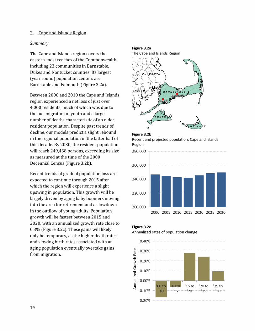
The Cape and Islands region covers the
eastern-most reaches of the Commonwealth,
including 23 communities in Barnstable,
Dukes and Nantucket counties. Its largest
(year round) population centers are
Barnstable and Falmouth (Figure 3.2a).
Between 2000 and 2010 the Cape and Islands
region experienced a net loss of just over
4,000 residents, much of which was due to
the out-migration of youth and a large
number of deaths characteristic of an older
resident population. Despite past trends of
decline, our models predict a slight rebound
in the regional population in the latter half of
this decade. By 2030, the resident population
will reach 249,438 persons, exceeding its size
as measured at the time of the 2000
Decennial Census (Figure 3.2b).
Recent trends of gradual population loss are
expected to continue through 2015 after
which the region will experience a slight
upswing in population. This growth will be
largely driven by aging baby boomers moving
into the area for retirement and a slowdown
in the outflow of young adults. Population
growth will be fastest between 2015 and
2020, with an annualized growth rate close to
0.3% (Figure 3.2c). These gains will likely
only be temporary, as the higher death rates
and slowing birth rates associated with an
aging population eventually overtake gains
from migration.
Figure 3.2b Recent and projected population, Cape and Islands Region
Figure 3.2c Annualized rates of population change
Figure 3.2a The Cape and Islands Region
20
The Sources of Population Change
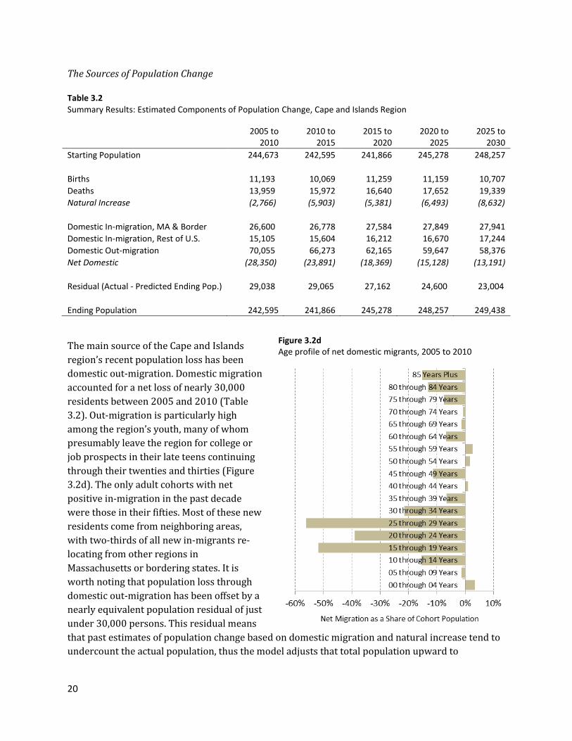
Table 3.2 Summary Results: Estimated Components of Population Change, Cape and Islands Region
2005 to
2010 2010 to
2015 2015 to
2020 2020 to
2025 2025 to
2030
Starting Population 244,673 242,595 241,866 245,278 248,257
Births 11,193 10,069 11,259 11,159 10,707
Deaths 13,959 15,972 16,640 17,652 19,339
Natural Increase (2,766) (5,903) (5,381) (6,493) (8,632)
Domestic In-migration, MA & Border 26,600 26,778 27,584 27,849 27,941
Domestic In-migration, Rest of U.S. 15,105 15,604 16,212 16,670 17,244
Domestic Out-migration 70,055 66,273 62,165 59,647 58,376
Net Domestic (28,350) (23,891) (18,369) (15,128) (13,191)
Residual (Actual - Predicted Ending Pop.) 29,038 29,065 27,162 24,600 23,004
Ending Population 242,595 241,866 245,278 248,257 249,438
The main source of the Cape and Islands
region’s recent population loss has been
domestic out-migration. Domestic migration
accounted for a net loss of nearly 30,000
residents between 2005 and 2010 (Table
3.2). Out-migration is particularly high
among the region’s youth, many of whom
presumably leave the region for college or
job prospects in their late teens continuing
through their twenties and thirties (Figure
3.2d). The only adult cohorts with net
positive in-migration in the past decade
were those in their fifties. Most of these new
residents come from neighboring areas,
with two-thirds of all new in-migrants re-
locating from other regions in
Massachusetts or bordering states. It is
worth noting that population loss through
domestic out-migration has been offset by a
nearly equivalent population residual of just
under 30,000 persons. This residual means
that past estimates of population change based on domestic migration and natural increase tend to
undercount the actual population, thus the model adjusts that total population upward to
Figure 3.2d Age profile of net domestic migrants, 2005 to 2010
21
compensate11. While we expect this residual to mainly reflect net international immigration, it also
captures prediction error associated with past components of change and thus is difficult to
interpret.
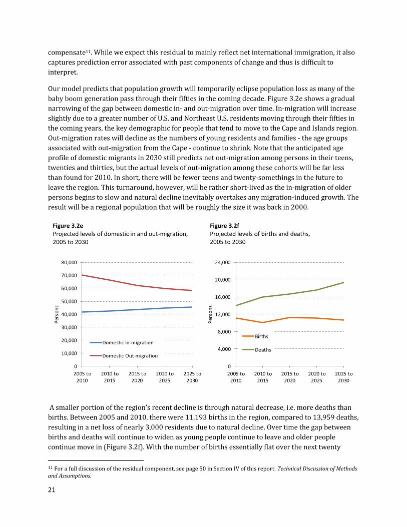
Our model predicts that population growth will temporarily eclipse population loss as many of the
baby boom generation pass through their fifties in the coming decade. Figure 3.2e shows a gradual
narrowing of the gap between domestic in- and out-migration over time. In-migration will increase
slightly due to a greater number of U.S. and Northeast U.S. residents moving through their fifties in
the coming years, the key demographic for people that tend to move to the Cape and Islands region.
Out-migration rates will decline as the numbers of young residents and families - the age groups
associated with out-migration from the Cape - continue to shrink. Note that the anticipated age
profile of domestic migrants in 2030 still predicts net out-migration among persons in their teens,
twenties and thirties, but the actual levels of out-migration among these cohorts will be far less
than found for 2010. In short, there will be fewer teens and twenty-somethings in the future to
leave the region. This turnaround, however, will be rather short-lived as the in-migration of older
persons begins to slow and natural decline inevitably overtakes any migration-induced growth. The
result will be a regional population that will be roughly the size it was back in 2000.
A smaller portion of the region’s recent decline is through natural decrease, i.e. more deaths than
births. Between 2005 and 2010, there were 11,193 births in the region, compared to 13,959 deaths,
resulting in a net loss of nearly 3,000 residents due to natural decline. Over time the gap between
births and deaths will continue to widen as young people continue to leave and older people
continue move in (Figure 3.2f). With the number of births essentially flat over the next twenty
11 For a full discussion of the residual component, see page 50 in Section IV of this report: Technical Discussion of Methods and Assumptions.
0
10,000
20,000
30,000
40,000
50,000
60,000
70,000
80,000
2005 to2010
2010 to2015
2015 to2020
2020 to2025
2025 to2030
Per
son
s
Domestic In-migration
Domestic Out-migration
0
4,000
8,000
12,000
16,000
20,000
24,000
2005 to2010
2010 to2015
2015 to2020
2020 to2025
2025 to2030
Per
son
s
Births
Deaths
Figure 3.2e Projected levels of domestic in and out-migration, 2005 to 2030
Figure 3.2f Projected levels of births and deaths, 2005 to 2030
22
20,000 10,000 0 10,000 20,000
00 through 04 Years
05 through 09 Years
10 through 14 Years
15 through 19 Years
20 through 24 Years
25 through 29 Years
30 through 34 Years
35 through 39 Years
40 through 44 Years
45 through 49 Years
50 through 54 Years
55 through 59 Years
60 through 64 Years
65 through 69 Years
70 through 74 Years
75 through 79 Years
80 through 84 Years
85 Years Plus
Persons
Females
Males
20,000 10,000 0 10,000 20,000
00 through 04 Years
05 through 09 Years
10 through 14 Years
15 through 19 Years
20 through 24 Years
25 through 29 Years
30 through 34 Years
35 through 39 Years
40 through 44 Years
45 through 49 Years
50 through 54 Years
55 through 59 Years
60 through 64 Years
65 through 69 Years
70 through 74 Years
75 through 79 Years
80 through 84 Years
85 Years Plus
Persons
2010 2030
years, the gap between deaths and births will continue to widen. By the 2025-30 period, the region
should expect a near 2:1 ratio of deaths over births with 19,339 deaths compared to 10,707 births.
A longer time horizon (i.e. 2040, 2050) would like show an even greater rise in regional deaths, and
likely a return to negative population growth, as the great population mass of baby boomers moves
into their seventies and eighties, where mortality rates rise considerably.
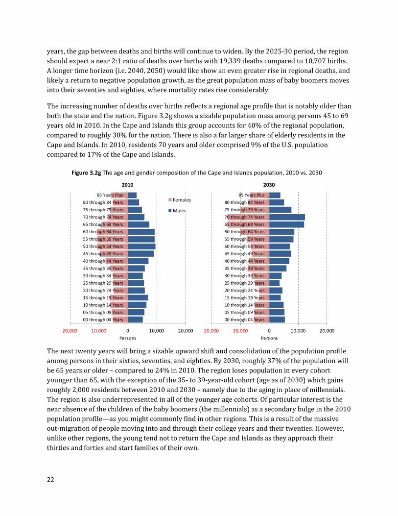
The increasing number of deaths over births reflects a regional age profile that is notably older than
both the state and the nation. Figure 3.2g shows a sizable population mass among persons 45 to 69
years old in 2010. In the Cape and Islands this group accounts for 40% of the regional population,
compared to roughly 30% for the nation. There is also a far larger share of elderly residents in the
Cape and Islands. In 2010, residents 70 years and older comprised 9% of the U.S. population
compared to 17% of the Cape and Islands.
The next twenty years will bring a sizable upward shift and consolidation of the population profile
among persons in their sixties, seventies, and eighties. By 2030, roughly 37% of the population will
be 65 years or older – compared to 24% in 2010. The region loses population in every cohort
younger than 65, with the exception of the 35- to 39-year-old cohort (age as of 2030) which gains
roughly 2,000 residents between 2010 and 2030 – namely due to the aging in place of millennials.
The region is also underrepresented in all of the younger age cohorts. Of particular interest is the
near absence of the children of the baby boomers (the millennials) as a secondary bulge in the 2010
population profile—as you might commonly find in other regions. This is a result of the massive
out-migration of people moving into and through their college years and their twenties. However,
unlike other regions, the young tend not to return the Cape and Islands as they approach their
thirties and forties and start families of their own.
Figure 3.2g The age and gender composition of the Cape and Islands population, 2010 vs. 2030
23
3. Central Region
Summary
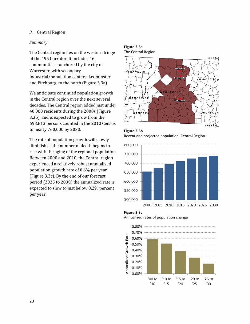
The Central region lies on the western fringe
of the 495 Corridor. It includes 46
communities—anchored by the city of
Worcester, with secondary
industrial/population centers, Leominster
and Fitchburg, to the north (Figure 3.3a).
We anticipate continued population growth
in the Central region over the next several
decades. The Central region added just under
40,000 residents during the 2000s (Figure
3.3b), and is expected to grow from the
693,813 persons counted in the 2010 Census
to nearly 760,000 by 2030.
The rate of population growth will slowly
diminish as the number of death begins to
rise with the aging of the regional population.
Between 2000 and 2010, the Central region
experienced a relatively robust annualized
population growth rate of 0.6% per year
(Figure 3.3c). By the end of our forecast
period (2025 to 2030) the annualized rate is
expected to slow to just below 0.2% percent
per year.
Figure 3.3b Recent and projected population, Central Region
Figure 3.3c Annualized rates of population change
Figure 3.3a The Central Region
24
The Sources of Population Change
Table 3.3 Summary Results: Estimated Components of Population Change, Central Region
2005 to 2010
2010 to 2015
2015 to 2020
2020 to 2025
2025 to 2030
Starting Population 674,238 693,813 711,671 725,295 735,150
Births 42,155 41,444 41,912 41,909 41,222
Deaths 28,966 32,119 33,849 35,966 39,081
Natural Increase 13,189 9,325 8,063 5,943 2,141
Domestic In-migration, MA & Border 99,475 97,413 99,343 98,519 97,997
Domestic In-migration, Rest of U.S. 28,920 28,877 29,619 30,358 31,251
Domestic Out-migration 120,590 118,246 120,876 120,580 119,281
Net Domestic 7,805 8,044 8,086 8,297 9,967
Residual (Actual - Predicted Ending Pop.) -1,419 489 -2,525 -4,385 -5,833
Ending Population 693,813 711,671 725,295 735,150 741,425
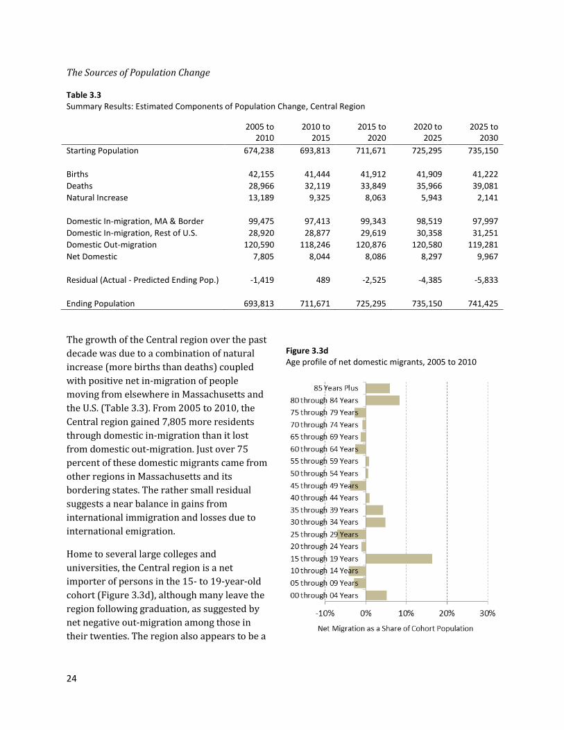
The growth of the Central region over the past
decade was due to a combination of natural
increase (more births than deaths) coupled
with positive net in-migration of people
moving from elsewhere in Massachusetts and
the U.S. (Table 3.3). From 2005 to 2010, the
Central region gained 7,805 more residents
through domestic in-migration than it lost
from domestic out-migration. Just over 75
percent of these domestic migrants came from
other regions in Massachusetts and its
bordering states. The rather small residual
suggests a near balance in gains from
international immigration and losses due to
international emigration.
Home to several large colleges and
universities, the Central region is a net
importer of persons in the 15- to 19-year-old
cohort (Figure 3.3d), although many leave the
region following graduation, as suggested by
net negative out-migration among those in
their twenties. The region also appears to be a
Figure 3.3d Age profile of net domestic migrants, 2005 to 2010
25
relatively attractive destination for elderly persons and those in their thirties—many of whom are
families with young children.
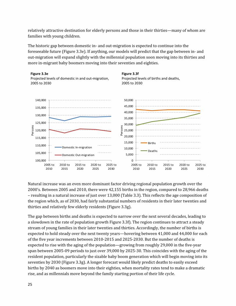
The historic gap between domestic in- and out-migration is expected to continue into the
foreseeable future (Figure 3.3e). If anything, our models will predict that the gap between in- and
out-migration will expand slightly with the millennial population soon moving into its thirties and
more in-migrant baby boomers moving into their seventies and eighties.
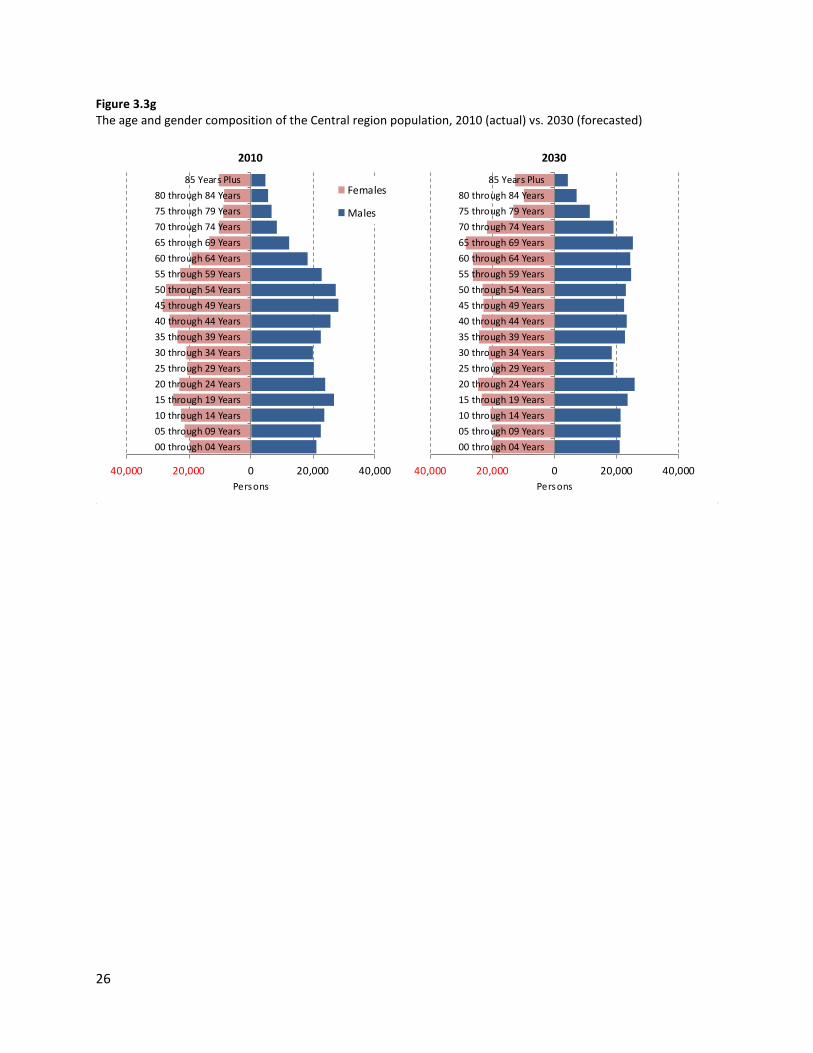
Natural increase was an even more dominant factor driving regional population growth over the
2000’s. Between 2005 and 2010, there were 42,155 births in the region, compared to 28,966 deaths
– resulting in a natural increase of just over 13,000 (Table 3.3). This reflects the age composition of
the region which, as of 2030, had fairly substantial numbers of residents in their later twenties and
thirties and relatively few elderly residents (Figure 3.3g).
The gap between births and deaths is expected to narrow over the next several decades, leading to
a slowdown in the rate of population growth Figure 3.3f). The region continues to attract a steady
stream of young families in their later twenties and thirties. Accordingly, the number of births is
expected to hold steady over the next twenty years—hovering between 41,000 and 44,000 for each
of the five year increments between 2010-2015 and 2025-2030. But the number of deaths is
expected to rise with the aging of the population—growing from roughly 29,000 in the five-year
span between 2005-09 periods to just over 39,000 by 2025-30. This coincides with the aging of the
resident population, particularly the sizable baby boom generation which will begin moving into its
seventies by 2030 (Figure 3.3g). A longer forecast would likely predict deaths to easily exceed
births by 2040 as boomers move into their eighties, when mortality rates tend to make a dramatic
rise, and as millennials move beyond the family starting portion of their life cycle.
100,000
105,000
110,000
115,000
120,000
125,000
130,000
135,000
140,000
2005 to2010
2010 to2015
2015 to2020
2020 to2025
2025 to2030
Per
son
s
Domestic In-migration
Domestic Out-migration
0
5,000
10,000
15,000
20,000
25,000
30,000
35,000
40,000
45,000
50,000
2005 to2010
2010 to2015
2015 to2020
2020 to2025
2025 to2030
Per
son
s
Births
Deaths
Figure 3.3e Projected levels of domestic in and out-migration, 2005 to 2030
Figure 3.3f Projected levels of births and deaths, 2005 to 2030
26
40,000 20,000 0 20,000 40,000
00 through 04 Years
05 through 09 Years
10 through 14 Years
15 through 19 Years
20 through 24 Years
25 through 29 Years
30 through 34 Years
35 through 39 Years
40 through 44 Years
45 through 49 Years
50 through 54 Years
55 through 59 Years
60 through 64 Years
65 through 69 Years
70 through 74 Years
75 through 79 Years
80 through 84 Years
85 Years Plus
Persons
Females
Males
40,000 20,000 0 20,000 40,000
00 through 04 Years
05 through 09 Years
10 through 14 Years
15 through 19 Years
20 through 24 Years
25 through 29 Years
30 through 34 Years
35 through 39 Years
40 through 44 Years
45 through 49 Years
50 through 54 Years
55 through 59 Years
60 through 64 Years
65 through 69 Years
70 through 74 Years
75 through 79 Years
80 through 84 Years
85 Years Plus
Persons
2010 2030
Figure 3.3g The age and gender composition of the Central region population, 2010 (actual) vs. 2030 (forecasted)

27
4. Greater Boston Region
Summary
The Greater Boston region is the major
employment and population center of the
Commonwealth of Massachusetts. It covers
the entirety of Suffolk County, and extends
into portions of Middlesex, Norfolk, and
Essex counties. There are 36 municipalities
in the Greater Boston region, including the
cities of Boston, Cambridge, Quincy and
Newton (Figure 3.4a).
Our long-term forecasts predict a steady
increase in the Greater Boston population
over the next 20 years, adding nearly
150,000 additional residents between 2010
and 2030 (Figure 3.4b). Population change in
the Greater Boston region is driven by
migration—particularly by the in-migration
young adults. Population growth will be
fastest in the next few years (Figure 3.4c) as
the swell of millennials (the children of the
baby boom generation) moves into and
through their twenties. The region tends to
lose residents to out-migration as they move
through the family-building and retirement
phases of life. Therefore, we expect
population growth to slow in the 2020s as
the millennials age into their thirties and
early forties and more baby boomers enter
their sixties and seventies. However, the
region’s population will continue to grow
during this time – albeit at a slower pace—as
international immigration and steady
increases in births will more than offset
population loss associated with domestic
out-migration and a slight increase in the
number of resident deaths.
Figure 3.4b Projected Population, Greater Boston Region
Figure 3.4a The Greater Boston Region
Figure 3.4c Annualized rates of population change
28
The Sources of Population Change
Table 3.4 Summary Results: Estimated Components of Population Change, Greater Boston Region
2005 to
2010 2010 to
2015 2015 to
2020 2020 to
2025 2025 to
2030
Starting Population 1,945,942 1,975,155 2,024,808 2,081,182 2,109,264
Births 122,374 123,710 132,135 136,953 136,705
Deaths 71,113 78,338 79,705 82,028 86,055
Natural Increase 51,261
45,372
52,430
54,925
50,650
Domestic In-migration, MA and Border States 303,920 308,034 330,303 324,015 318,746
Domestic In-migration, Rest of U.S. 222,590 224,963 230,705 234,369 238,223
Domestic Out-migration 547,465 530,536 552,980 567,474 569,114
Net Domestic -20,955 2,461 8,028 -9,090 -12,145
Immigration (International) 153,105 145,506 151,274 156,502 156,701
Residual (Actual - Predicted Pop. Ending) -154,198 -143,686 -155,359 -174,255 -181,217
Ending Population 1,975,155 2,024,808 2,081,182 2,109,264 2,123,253
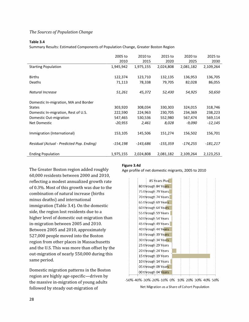
The Greater Boston region added roughly
60,000 residents between 2000 and 2010,
reflecting a modest annualized growth rate
of 0.3%. Most of this growth was due to the
combination of natural increase (births
minus deaths) and international
immigration (Table 3.4). On the domestic
side, the region lost residents due to a
higher level of domestic out-migration than
in-migration between 2005 and 2010.
Between 2005 and 2010, approximately
527,000 people moved into the Boston
region from other places in Massachusetts
and the U.S. This was more than offset by the
out-migration of nearly 550,000 during this
same period.
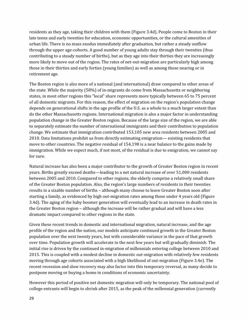
Domestic migration patterns in the Boston
region are highly age-specific—driven by
the massive in-migration of young adults
followed by steady out-migration of
Figure 3.4d Age profile of net domestic migrants, 2005 to 2010
29
residents as they age, taking their children with them (Figure 3.4d). People come to Boston in their
late teens and early twenties for education, economic opportunities, or the cultural amenities of
urban life. There is no mass exodus immediately after graduation, but rather a steady outflow
through the upper age-cohorts. A good number of young adults stay through their twenties (thus
contributing to a steady number of births), but as they age into their thirties they are increasingly
more likely to move out of the region. The rates of net-out-migration are particularly high among
those in their thirties and early forties (young families) as well as among those nearing or in
retirement age.
The Boston region is also more of a national (and international) draw compared to other areas of
the state. While the majority (58%) of in-migrants do come from Massachusetts or neighboring
states, in most other regions this “local” share represents more typically between 65 to 75 percent
of all domestic migrants. For this reason, the effect of migration on the region’s population change
depends on generational shifts in the age profile of the U.S. as a whole to a much larger extent than
do the other Massachusetts regions. International migration is also a major factor in understanding
population change in the Greater Boston region. Because of the large size of the region, we are able
to separately estimate the number of international immigrants and their contribution to population
change. We estimate that immigration contributed 153,105 new area residents between 2005 and
2010. Data limitations prohibit us from directly estimating emigration— existing residents that
move to other countries. The negative residual of 154,198 is a near balance to the gains made by
immigration. While we expect much, if not most, of the residual is due to emigration, we cannot say
for sure.
Natural increase has also been a major contributor to the growth of Greater Boston region in recent
years. Births greatly exceed deaths—leading to a net natural increase of over 51,000 residents
between 2005 and 2010. Compared to other regions, the elderly comprise a relatively small share
of the Greater Boston population. Also, the region’s large numbers of residents in their twenties
results in a sizable number of births – although many choose to leave Greater Boston soon after
starting a family, as evidenced by high out-migration rates among those under 4 years old (Figure
3.4d). The aging of the baby boomer generation will eventually lead to an increase in death rates in
the Greater Boston region – although the increase will be rather gradual and will have a less
dramatic impact compared to other regions in the state.
Given these recent trends in domestic and international migration, natural increase, and the age
profile of the region and the nation, our models anticipate continued growth in the Greater Boston
population over the next twenty years, but with considerable variance in the pace of that growth
over time. Population growth will accelerate in the next few years but will gradually diminish. The
initial rise is driven by the continued in-migration of millennials entering college between 2010 and
2015. This is coupled with a modest decline in domestic out-migration with relatively few residents
moving through age cohorts associated with a high likelihood of out-migration (Figure 3.4e). The
recent recession and slow recovery may also factor into this temporary reversal, as many decide to
postpone moving or buying a home in conditions of economic uncertainty.
However this period of positive net domestic migration will only be temporary. The national pool of
college entrants will begin to shrink after 2015, as the peak of the millennial generation (currently
30
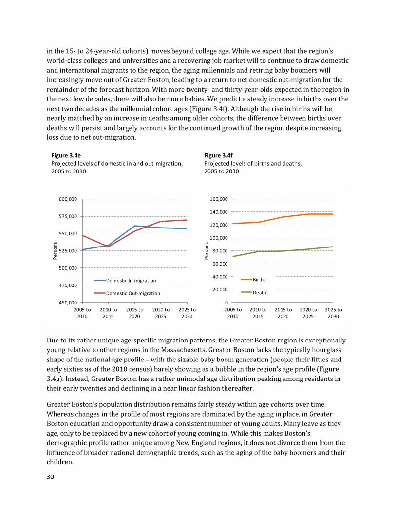
in the 15- to 24-year-old cohorts) moves beyond college age. While we expect that the region’s
world-class colleges and universities and a recovering job market will to continue to draw domestic
and international migrants to the region, the aging millennials and retiring baby boomers will
increasingly move out of Greater Boston, leading to a return to net domestic out-migration for the
remainder of the forecast horizon. With more twenty- and thirty-year-olds expected in the region in
the next few decades, there will also be more babies. We predict a steady increase in births over the
next two decades as the millennial cohort ages (Figure 3.4f). Although the rise in births will be
nearly matched by an increase in deaths among older cohorts, the difference between births over
deaths will persist and largely accounts for the continued growth of the region despite increasing
loss due to net out-migration.
Due to its rather unique age-specific migration patterns, the Greater Boston region is exceptionally
young relative to other regions in the Massachusetts. Greater Boston lacks the typically hourglass
shape of the national age profile – with the sizable baby boom generation (people their fifties and
early sixties as of the 2010 census) barely showing as a bubble in the region’s age profile (Figure
3.4g). Instead, Greater Boston has a rather unimodal age distribution peaking among residents in
their early twenties and declining in a near linear fashion thereafter.
Greater Boston’s population distribution remains fairly steady within age cohorts over time.
Whereas changes in the profile of most regions are dominated by the aging in place, in Greater
Boston education and opportunity draw a consistent number of young adults. Many leave as they
age, only to be replaced by a new cohort of young coming in. While this makes Boston’s
demographic profile rather unique among New England regions, it does not divorce them from the
influence of broader national demographic trends, such as the aging of the baby boomers and their
children.
450,000
475,000
500,000
525,000
550,000
575,000
600,000
2005 to2010
2010 to2015
2015 to2020
2020 to2025
2025 to2030
Per
son
s
Domestic In-migration
Domestic Out-migration
0
20,000
40,000
60,000
80,000
100,000
120,000
140,000
160,000
2005 to2010
2010 to2015
2015 to2020
2020 to2025
2025 to2030
Per
son
s
Births
Deaths
Figure 3.4e Projected levels of domestic in and out-migration, 2005 to 2030
Figure 3.4f Projected levels of births and deaths, 2005 to 2030
31
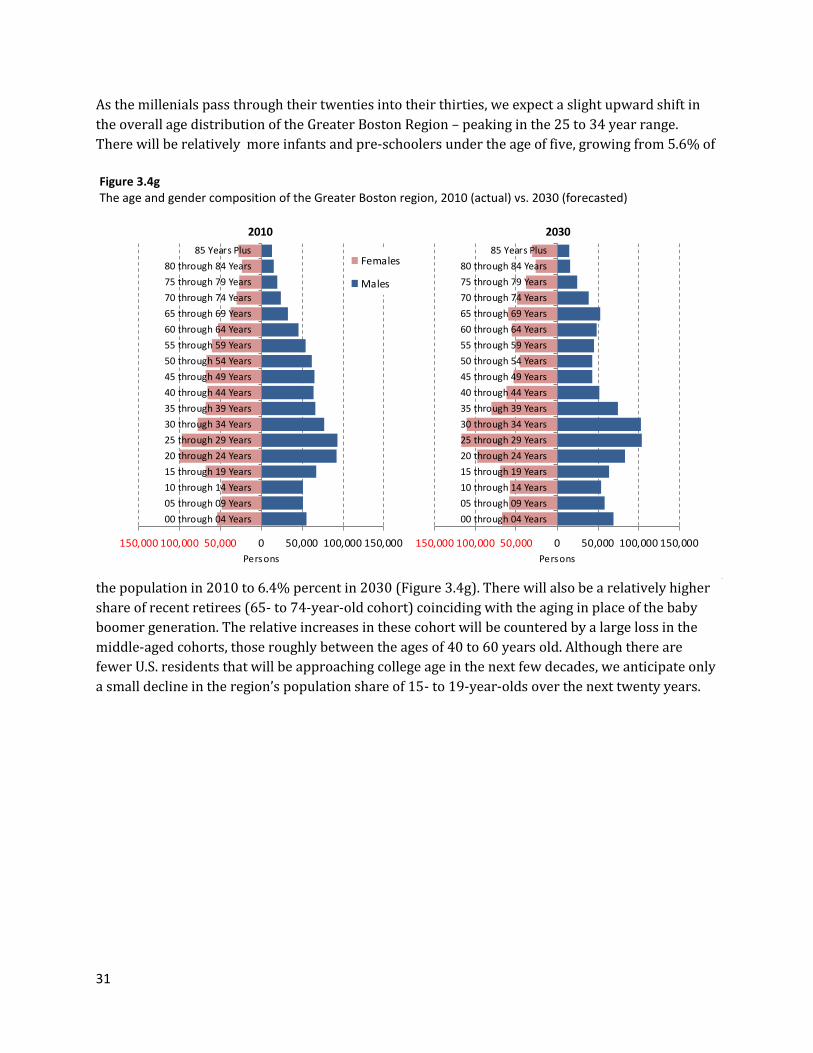
As the millenials pass through their twenties into their thirties, we expect a slight upward shift in
the overall age distribution of the Greater Boston Region – peaking in the 25 to 34 year range.
There will be relatively more infants and pre-schoolers under the age of five, growing from 5.6% of
the population in 2010 to 6.4% percent in 2030 (Figure 3.4g). There will also be a relatively higher
share of recent retirees (65- to 74-year-old cohort) coinciding with the aging in place of the baby
boomer generation. The relative increases in these cohort will be countered by a large loss in the
middle-aged cohorts, those roughly between the ages of 40 to 60 years old. Although there are
fewer U.S. residents that will be approaching college age in the next few decades, we anticipate only
a small decline in the region’s population share of 15- to 19-year-olds over the next twenty years.
150,000 100,000 50,000 0 50,000 100,000 150,000
00 through 04 Years
05 through 09 Years
10 through 14 Years
15 through 19 Years
20 through 24 Years
25 through 29 Years
30 through 34 Years
35 through 39 Years
40 through 44 Years
45 through 49 Years
50 through 54 Years
55 through 59 Years
60 through 64 Years
65 through 69 Years
70 through 74 Years
75 through 79 Years
80 through 84 Years
85 Years Plus
Persons
Females
Males
150,000 100,000 50,000 0 50,000 100,000 150,000
00 through 04 Years
05 through 09 Years
10 through 14 Years
15 through 19 Years
20 through 24 Years
25 through 29 Years
30 through 34 Years
35 through 39 Years
40 through 44 Years
45 through 49 Years
50 through 54 Years
55 through 59 Years
60 through 64 Years
65 through 69 Years
70 through 74 Years
75 through 79 Years
80 through 84 Years
85 Years Plus
Persons
2010 2030
Figure 3.4g The age and gender composition of the Greater Boston region, 2010 (actual) vs. 2030 (forecasted)
32
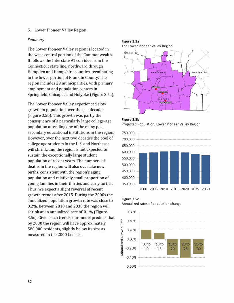
5. Lower Pioneer Valley Region
Summary
The Lower Pioneer Valley region is located in
the west-central portion of the Commonwealth.
It follows the Interstate 91 corridor from the
Connecticut state line, northward through
Hampden and Hampshire counties, terminating
in the lower portion of Franklin County. The
region includes 29 municipalities, with primary
employment and population centers in
Springfield, Chicopee and Holyoke (Figure 3.5a).
The Lower Pioneer Valley experienced slow
growth in population over the last decade
(Figure 3.5b). This growth was partly the
consequence of a particularly large college-age
population attending one of the many post-
secondary educational institutions in the region.
However, over the next two decades the pool of
college age students in the U.S. and Northeast
will shrink, and the region is not expected to
sustain the exceptionally large student
population of recent years. The numbers of
deaths in the region will also overtake new
births, consistent with the region’s aging
population and relatively small proportion of
young families in their thirties and early forties.
Thus, we expect a slight reversal of recent
growth trends after 2015. During the 2000s the
annualized population growth rate was close to
0.2%. Between 2010 and 2030 the region will
shrink at an annualized rate of-0.1% (Figure
3.5c). Given such trends, our model predicts that
by 2030 the region will have approximately
580,000 residents, slightly below its size as
measured in the 2000 Census.
Figure 3.5b Projected Population, Lower Pioneer Valley Region
Figure 3.5a The Lower Pioneer Valley Region
Figure 3.5c Annualized rates of population change

33
The Sources of Population Change
Table 3.5 Summary Results: Estimated Components of Population Change, Lower Pioneer Valley Region
2005 to 2010
2010 to 2015
2015 to 2020
2020 to 2025
2025 to 2030
Starting Population 598,128 604,304 608,446 598,040 585,918
Births 33,827 34,829 29,006 28,022 27,701
Deaths 26,748 29,507 30,081 31,120 33,063
Natural Increase 7,079 5,322 -1,075 -3,098 -5,362
Domestic In-migration, MA & Border 83,410 82,029 81,798 80,523 80,396
Domestic In-migration, Rest of U.S. 46,745 46,958 47,911 48,695 49,841
Domestic Out-migration 103,320 103,326 107,849 105,520 102,560
Net Domestic 26,835 25,661 21,860 23,698 27,677
Residual (Actual - Predicted Ending Pop.) -27,738 -26,841 -31,191 -32,722 -31,687
Ending Population 604,304 608,446 598,040 585,918 576,546
The Lower Pioneer Valley region added
just over 12,000 residents between 2000
and 2010 – due to a combination of natural
increase (more births than deaths) and net
domestic in-migration (Table 3.5).
Domestic migration is heavily
concentrated among college age students.
More than 50% of all domestic in-migrants
between 2005 and 2010 were between 15
and 25 years old (Figure 3.5d). However, a
large number leave the region after
completing their studies –reflected by a
net migration rate closer to zero in the 20
to 24 year cohorts and a negative net
migration rate among those 25 to 39 years
of age. The sizable student population
results in a higher portion of domestic in-
migrants coming from outside the
Northeast. Between 2005 and 2010, 64%
of all domestic in-migrants came from
Massachusetts or one of its bordering
Figure 3.5d Age profile of net domestic migrants, 2005 to 2010
34
states. Although a majority, this share is among the lowest of all regions in the state. Therefore, the
future size of the region is heavily influenced by not only regional demographic trends, but also
national and international ones.
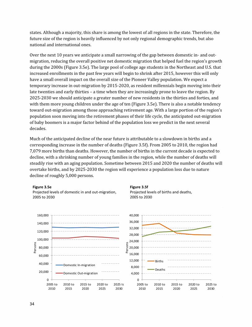
Over the next 10 years we anticipate a small narrowing of the gap between domestic in- and out-
migration, reducing the overall positive net domestic migration that helped fuel the region’s growth
during the 2000s (Figure 3.5e). The large pool of college age students in the Northeast and U.S. that
increased enrollments in the past few years will begin to shrink after 2015, however this will only
have a small overall impact on the overall size of the Pioneer Valley population. We expect a
temporary increase in out-migration by 2015-2020, as resident millennials begin moving into their
late twenties and early thirties – a time when they are increasingly prone to leave the region. By
2025-2030 we should anticipate a greater number of new residents in the thirties and forties, and
with them more young children under the age of ten (Figure 3.5e). There is also a notable tendency
toward out-migration among those approaching retirement age. With a large portion of the region’s
population soon moving into the retirement phases of their life cycle, the anticipated out-migration
of baby boomers is a major factor behind of the population loss we predict in the next several
decades.
Much of the anticipated decline of the near future is attributable to a slowdown in births and a
corresponding increase in the number of deaths (Figure 3.5f). From 2005 to 2010, the region had
7,079 more births than deaths. However, the number of births in the current decade is expected to
decline, with a shrinking number of young families in the region, while the number of deaths will
steadily rise with an aging population. Sometime between 2015 and 2020 the number of deaths will
overtake births, and by 2025-2030 the region will experience a population loss due to nature
decline of roughly 5,000 persons.
0
20,000
40,000
60,000
80,000
100,000
120,000
140,000
160,000
2005 to2010
2010 to2015
2015 to2020
2020 to2025
2025 to2030
Per
son
s
Domestic In-migration
Domestic Out-migration
0
4,000
8,000
12,000
16,000
20,000
24,000
28,000
32,000
36,000
40,000
2005 to2010
2010 to2015
2015 to2020
2020 to2025
2025 to2030
Per
son
s
Births
Deaths
Figure 3.5e Projected levels of domestic in and out-migration, 2005 to 2030
Figure 3.5f Projected levels of births and deaths, 2005 to 2030
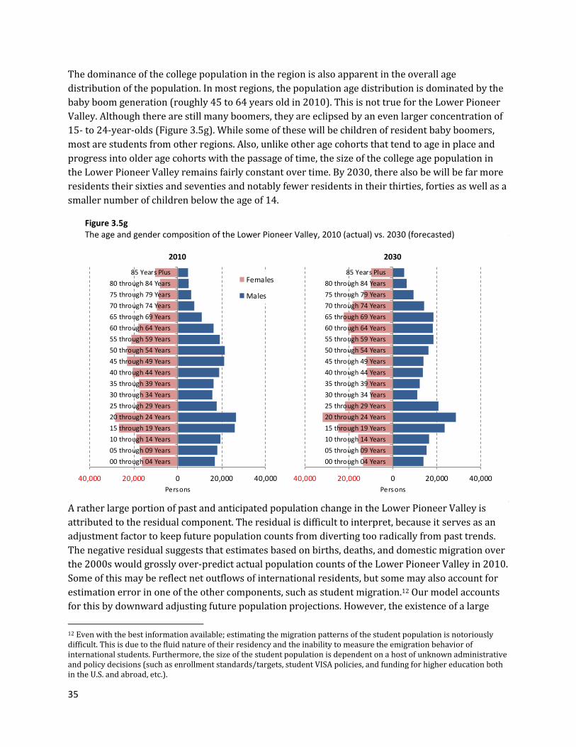
35
The dominance of the college population in the region is also apparent in the overall age
distribution of the population. In most regions, the population age distribution is dominated by the
baby boom generation (roughly 45 to 64 years old in 2010). This is not true for the Lower Pioneer
Valley. Although there are still many boomers, they are eclipsed by an even larger concentration of
15- to 24-year-olds (Figure 3.5g). While some of these will be children of resident baby boomers,
most are students from other regions. Also, unlike other age cohorts that tend to age in place and
progress into older age cohorts with the passage of time, the size of the college age population in
the Lower Pioneer Valley remains fairly constant over time. By 2030, there also be will be far more
residents their sixties and seventies and notably fewer residents in their thirties, forties as well as a
smaller number of children below the age of 14.
A rather large portion of past and anticipated population change in the Lower Pioneer Valley is
attributed to the residual component. The residual is difficult to interpret, because it serves as an
adjustment factor to keep future population counts from diverting too radically from past trends.
The negative residual suggests that estimates based on births, deaths, and domestic migration over
the 2000s would grossly over-predict actual population counts of the Lower Pioneer Valley in 2010.
Some of this may be reflect net outflows of international residents, but some may also account for
estimation error in one of the other components, such as student migration.12 Our model accounts
for this by downward adjusting future population projections. However, the existence of a large
12 Even with the best information available; estimating the migration patterns of the student population is notoriously difficult. This is due to the fluid nature of their residency and the inability to measure the emigration behavior of international students. Furthermore, the size of the student population is dependent on a host of unknown administrative and policy decisions (such as enrollment standards/targets, student VISA policies, and funding for higher education both in the U.S. and abroad, etc.).
40,000 20,000 0 20,000 40,000
00 through 04 Years
05 through 09 Years
10 through 14 Years
15 through 19 Years
20 through 24 Years
25 through 29 Years
30 through 34 Years
35 through 39 Years
40 through 44 Years
45 through 49 Years
50 through 54 Years
55 through 59 Years
60 through 64 Years
65 through 69 Years
70 through 74 Years
75 through 79 Years
80 through 84 Years
85 Years Plus
Persons
Females
Males
40,000 20,000 0 20,000 40,000
00 through 04 Years
05 through 09 Years
10 through 14 Years
15 through 19 Years
20 through 24 Years
25 through 29 Years
30 through 34 Years
35 through 39 Years
40 through 44 Years
45 through 49 Years
50 through 54 Years
55 through 59 Years
60 through 64 Years
65 through 69 Years
70 through 74 Years
75 through 79 Years
80 through 84 Years
85 Years Plus
Persons
2010 2030
Figure 3.5g The age and gender composition of the Lower Pioneer Valley, 2010 (actual) vs. 2030 (forecasted)

36
residual should serve as a warning against a strict interpretation of our long-term projections as
definite.
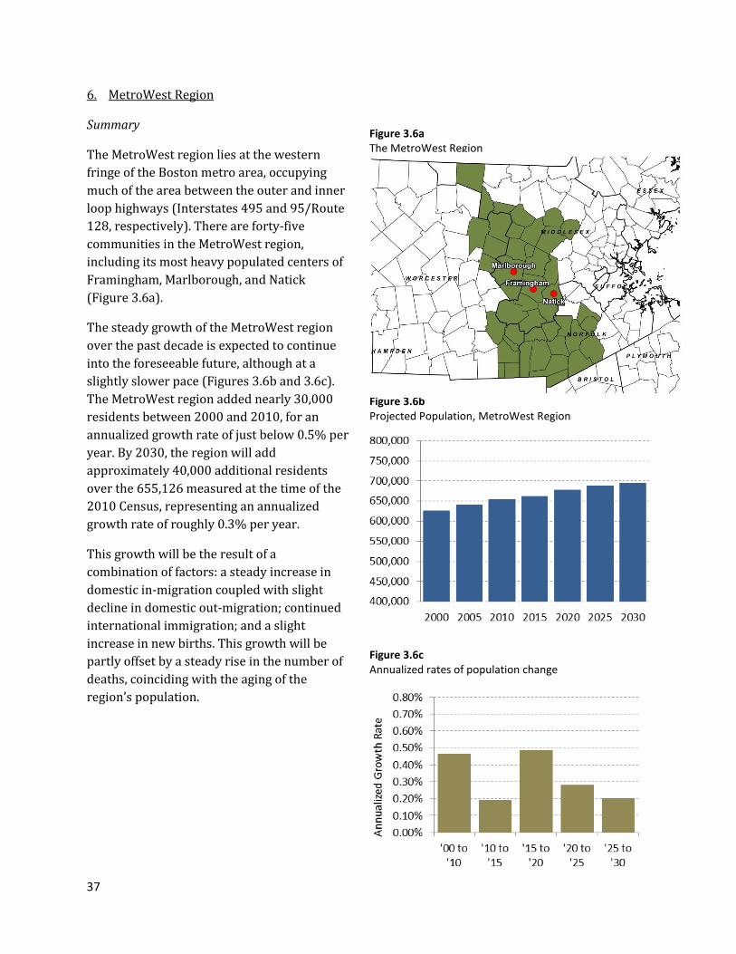
37
6. MetroWest Region
Summary
The MetroWest region lies at the western
fringe of the Boston metro area, occupying
much of the area between the outer and inner
loop highways (Interstates 495 and 95/Route
128, respectively). There are forty-five
communities in the MetroWest region,
including its most heavy populated centers of
Framingham, Marlborough, and Natick
(Figure 3.6a).
The steady growth of the MetroWest region
over the past decade is expected to continue
into the foreseeable future, although at a
slightly slower pace (Figures 3.6b and 3.6c).
The MetroWest region added nearly 30,000
residents between 2000 and 2010, for an
annualized growth rate of just below 0.5% per
year. By 2030, the region will add
approximately 40,000 additional residents
over the 655,126 measured at the time of the
2010 Census, representing an annualized
growth rate of roughly 0.3% per year.
This growth will be the result of a
combination of factors: a steady increase in
domestic in-migration coupled with slight
decline in domestic out-migration; continued
international immigration; and a slight
increase in new births. This growth will be
partly offset by a steady rise in the number of
deaths, coinciding with the aging of the
region’s population.
Figure 3.6a The MetroWest Region
Figure 3.6b Projected Population, MetroWest Region
Figure 3.6c Annualized rates of population change
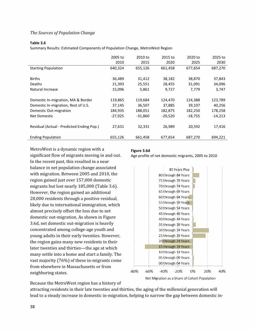
38
The Sources of Population Change
Table 3.6 Summary Results: Estimated Components of Population Change, MetroWest Region
2005 to 2010
2010 to 2015
2015 to 2020
2020 to 2025
2025 to 2030
Starting Population 640,324 655,126 661,458 677,654 687,270
Births 36,489 31,412 38,182 38,870 37,843
Deaths 21,393 25,551 28,455 31,091 34,096
Natural Increase 15,096 5,861 9,727 7,779 3,747
Domestic In-migration, MA & Border 119,865 119,684 124,470 124,388 123,789
Domestic In-migration, Rest of U.S. 37,145 36,507 37,885 39,107 40,256
Domestic Out-migration 184,935 188,051 182,875 182,250 178,258
Net Domestic -27,925 -31,860 -20,520 -18,755 -14,213
Residual (Actual - Predicted Ending Pop.) 27,631 32,331 26,989 20,592 17,416
Ending Population 655,126 661,458 677,654 687,270 694,221
MetroWest is a dynamic region with a
significant flow of migrants moving in and out.
In the recent past, this resulted in a near
balance in net population change associated
with migration. Between 2005 and 2010, the
region gained just over 157,000 domestic
migrants but lost nearly 185,000 (Table 3.6).
However, the region gained an additional
28,000 residents through a positive residual,
likely due to international immigration, which
almost precisely offset the loss due to net
domestic out-migration. As shown in Figure
3.6d, net domestic out-migration is heavily
concentrated among college-age youth and
young adults in their early twenties. However,
the region gains many new residents in their
later twenties and thirties—the age at which
many settle into a home and start a family. The
vast majority (76%) of these in-migrants come
from elsewhere in Massachusetts or from
neighboring states.
Because the MetroWest region has a history of
attracting residents in their late twenties and thirties, the aging of the millennial generation will
lead to a steady increase in domestic in-migration, helping to narrow the gap between domestic in-
Figure 3.6d Age profile of net domestic migrants, 2005 to 2010
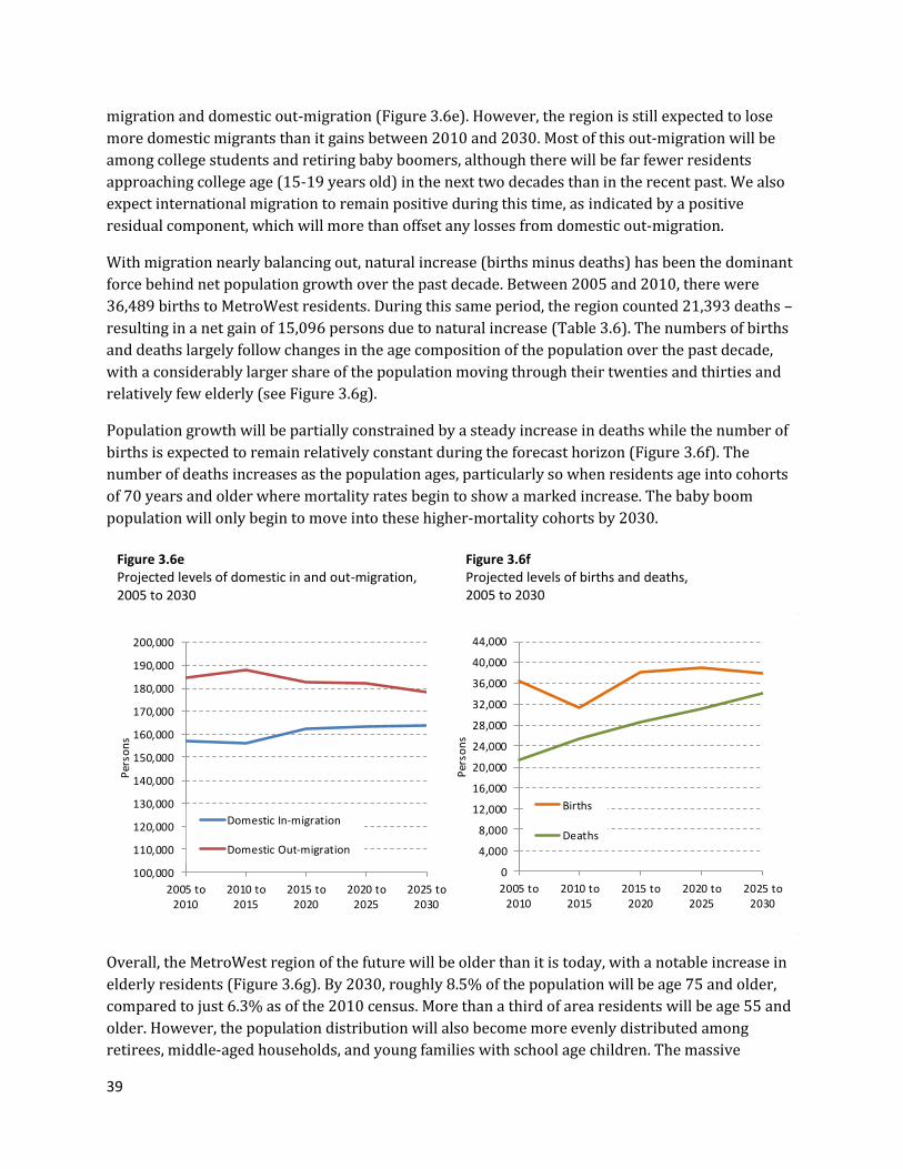
39
migration and domestic out-migration (Figure 3.6e). However, the region is still expected to lose
more domestic migrants than it gains between 2010 and 2030. Most of this out-migration will be
among college students and retiring baby boomers, although there will be far fewer residents
approaching college age (15-19 years old) in the next two decades than in the recent past. We also
expect international migration to remain positive during this time, as indicated by a positive
residual component, which will more than offset any losses from domestic out-migration.
With migration nearly balancing out, natural increase (births minus deaths) has been the dominant
force behind net population growth over the past decade. Between 2005 and 2010, there were
36,489 births to MetroWest residents. During this same period, the region counted 21,393 deaths –
resulting in a net gain of 15,096 persons due to natural increase (Table 3.6). The numbers of births
and deaths largely follow changes in the age composition of the population over the past decade,
with a considerably larger share of the population moving through their twenties and thirties and
relatively few elderly (see Figure 3.6g).
Population growth will be partially constrained by a steady increase in deaths while the number of
births is expected to remain relatively constant during the forecast horizon (Figure 3.6f). The
number of deaths increases as the population ages, particularly so when residents age into cohorts
of 70 years and older where mortality rates begin to show a marked increase. The baby boom
population will only begin to move into these higher-mortality cohorts by 2030.
Overall, the MetroWest region of the future will be older than it is today, with a notable increase in
elderly residents (Figure 3.6g). By 2030, roughly 8.5% of the population will be age 75 and older,
compared to just 6.3% as of the 2010 census. More than a third of area residents will be age 55 and
older. However, the population distribution will also become more evenly distributed among
retirees, middle-aged households, and young families with school age children. The massive
100,000
110,000
120,000
130,000
140,000
150,000
160,000
170,000
180,000
190,000
200,000
2005 to2010
2010 to2015
2015 to2020
2020 to2025
2025 to2030
Per
son
s
Domestic In-migration
Domestic Out-migration
0
4,000
8,000
12,000
16,000
20,000
24,000
28,000
32,000
36,000
40,000
44,000
2005 to2010
2010 to2015
2015 to2020
2020 to2025
2025 to2030
Per
son
s
Births
Deaths
Figure 3.6e Projected levels of domestic in and out-migration, 2005 to 2030
Figure 3.6f Projected levels of births and deaths, 2005 to 2030
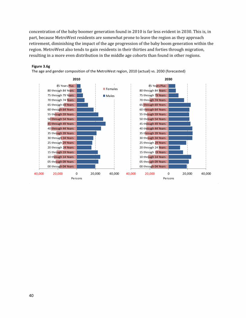
40
concentration of the baby boomer generation found in 2010 is far less evident in 2030. This is, in
part, because MetroWest residents are somewhat prone to leave the region as they approach
retirement, diminishing the impact of the age progression of the baby boom generation within the
region. MetroWest also tends to gain residents in their thirties and forties through migration,
resulting in a more even distribution in the middle age cohorts than found in other regions.
40,000 20,000 0 20,000 40,000
00 through 04 Years
05 through 09 Years
10 through 14 Years
15 through 19 Years
20 through 24 Years
25 through 29 Years
30 through 34 Years
35 through 39 Years
40 through 44 Years
45 through 49 Years
50 through 54 Years
55 through 59 Years
60 through 64 Years
65 through 69 Years
70 through 74 Years
75 through 79 Years
80 through 84 Years
85 Years Plus
Persons
Females
Males
40,000 20,000 0 20,000 40,000
00 through 04 Years
05 through 09 Years
10 through 14 Years
15 through 19 Years
20 through 24 Years
25 through 29 Years
30 through 34 Years
35 through 39 Years
40 through 44 Years
45 through 49 Years
50 through 54 Years
55 through 59 Years
60 through 64 Years
65 through 69 Years
70 through 74 Years
75 through 79 Years
80 through 84 Years
85 Years Plus
Persons
2010 2030
Figure 3.6g The age and gender composition of the MetroWest region, 2010 (actual) vs. 2030 (forecasted)
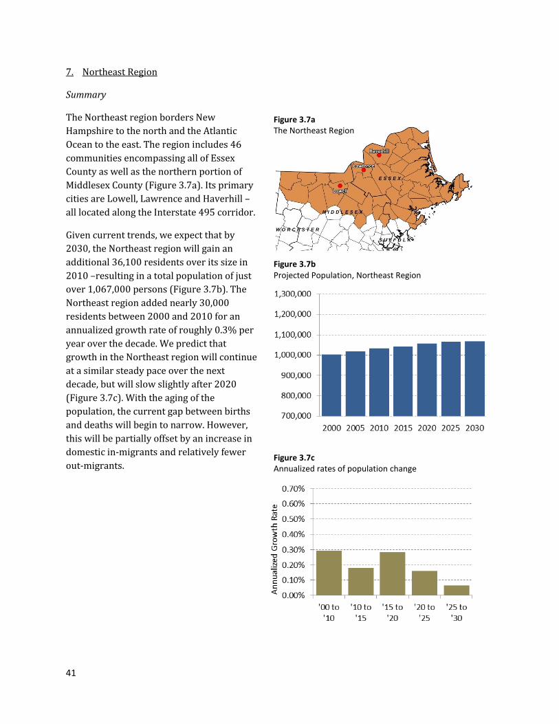
41
7. Northeast Region
Summary
The Northeast region borders New
Hampshire to the north and the Atlantic
Ocean to the east. The region includes 46
communities encompassing all of Essex
County as well as the northern portion of
Middlesex County (Figure 3.7a). Its primary
cities are Lowell, Lawrence and Haverhill –
all located along the Interstate 495 corridor.
Given current trends, we expect that by
2030, the Northeast region will gain an
additional 36,100 residents over its size in
2010 –resulting in a total population of just
over 1,067,000 persons (Figure 3.7b). The
Northeast region added nearly 30,000
residents between 2000 and 2010 for an
annualized growth rate of roughly 0.3% per
year over the decade. We predict that
growth in the Northeast region will continue
at a similar steady pace over the next
decade, but will slow slightly after 2020
(Figure 3.7c). With the aging of the
population, the current gap between births
and deaths will begin to narrow. However,
this will be partially offset by an increase in
domestic in-migrants and relatively fewer
out-migrants.
Figure 3.7c Annualized rates of population change
Figure 3.7b Projected Population, Northeast Region
Figure 3.7a The Northeast Region

42
The Sources of Population Change
Table 3.7 Summary Results: Estimated Components of Population Change, Northeast Region
2005 to
2010 2010 to
2015 2015 to
2020 2020 to
2025 2025 to
2030
Starting Population 1,016,886 1,031,733 1,041,018 1,055,889 1,064,326
Births 60,178 56,362 61,525 62,084 60,462
Deaths 40,098 46,144 49,836 53,515 58,149
Natural Increase 20,080
10,218
11,689 8,569 2,313
Domestic In-migration, MA and Border States
128,695 128,217 133,859 132,927 132,031
Domestic In-migration, Rest of U.S. 45,265 45,886 47,913 49,507 51,261
Domestic Out-migration 210,615 208,825 208,381 206,539 202,257
Net Domestic -36,655 -34,722 -26,609 -24,105 -18,965
Immigration (International) 22,530 19,706 20,309 20,545 20,696
Residual (Actual - Predicted Pop. Ending) 8,892 14,083 9,482 3,428 -537
Ending Population 1,031,733 1,041,018 1,055,889 1,064,326 1,067,833
In recent years, the Northeast region has lost
more residents to domestic migration than it
has gained (Table 3.7). Between 2005 and
2009, we estimate the number of domestic in-
migrants to be close to 174,000 persons, with
the bulk (74%) coming from either
Massachusetts or a neighboring state. During
this time the region also lost nearly 211,000
residents moving to other areas of the U.S. The
largest cohorts of out-migrants are the 15- to
24-year-olds, many of whom headed off to
college or to look for work opportunities
elsewhere (Figure 3.7d). Those approaching
retirement age are also somewhat prone to
move elsewhere in the U.S., although the
region tends to be a net importer of the
elderly. However, similar to other regions on
the fringe of the Boston Metropolitan area, the
Northeast is a net attractor of young families
and others in their early thirties.
Figure 3.7d Age profile of net domestic migrants, 2005 to 2010
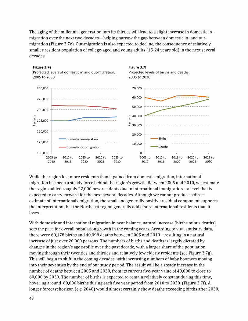
43
The aging of the millennial generation into its thirties will lead to a slight increase in domestic in-
migration over the next two decades—helping narrow the gap between domestic in- and out-
migration (Figure 3.7e). Out-migration is also expected to decline, the consequence of relatively
smaller resident population of college-aged and young adults (15-24 years old) in the next several
decades.
While the region lost more residents than it gained from domestic migration, international
migration has been a steady force behind the region’s growth. Between 2005 and 2010, we estimate
the region added roughly 22,000 new residents due to international immigration – a level that is
expected to carry forward for the next several decades. Although we cannot produce a direct
estimate of international emigration, the small and generally positive residual component supports
the interpretation that the Northeast region generally adds more international residents than it
loses.
With domestic and international migration in near balance, natural increase (births minus deaths)
sets the pace for overall population growth in the coming years. According to vital statistics data,
there were 60,178 births and 40,098 deaths between 2005 and 2010 – resulting in a natural
increase of just over 20,000 persons. The numbers of births and deaths is largely dictated by
changes in the region’s age profile over the past decade, with a larger share of the population
moving through their twenties and thirties and relatively few elderly residents (see Figure 3.7g).
This will begin to shift in the coming decades, with increasing numbers of baby boomers moving
into their seventies by the end of our study period. The result will be a steady increase in the
number of deaths between 2005 and 2030, from its current five-year value of 40,000 to close to
60,000 by 2030. The number of births is expected to remain relatively constant during this time,
hovering around 60,000 births during each five year period from 2010 to 2030 (Figure 3.7f). A
longer forecast horizon (e.g. 2040) would almost certainly show deaths exceeding births after 2030.
Figure 3.7e Projected levels of domestic in and out-migration, 2005 to 2030
Figure 3.7f Projected levels of births and deaths, 2005 to 2030
100,000
125,000
150,000
175,000
200,000
225,000
250,000
2005 to2010
2010 to2015
2015 to2020
2020 to2025
2025 to2030
Per
son
s
Domestic In-migration
Domestic Out-migration
0
10,000
20,000
30,000
40,000
50,000
60,000
70,000
2005 to2010
2010 to2015
2015 to2020
2020 to2025
2025 to2030
Per
son
s
Births
Deaths
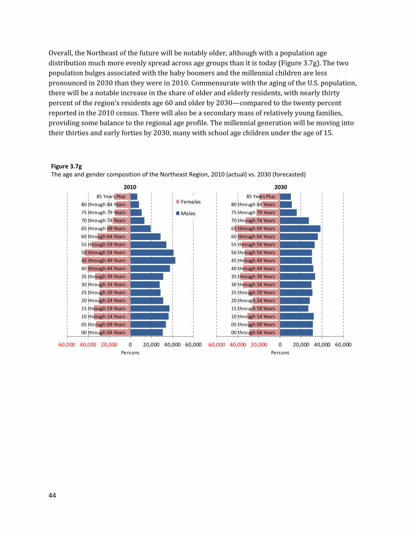
44
Overall, the Northeast of the future will be notably older, although with a population age
distribution much more evenly spread across age groups than it is today (Figure 3.7g). The two
population bulges associated with the baby boomers and the millennial children are less
pronounced in 2030 than they were in 2010. Commensurate with the aging of the U.S. population,
there will be a notable increase in the share of older and elderly residents, with nearly thirty
percent of the region’s residents age 60 and older by 2030—compared to the twenty percent
reported in the 2010 census. There will also be a secondary mass of relatively young families,
providing some balance to the regional age profile. The millennial generation will be moving into
their thirties and early forties by 2030, many with school age children under the age of 15.
Figure 3.7g The age and gender composition of the Northeast Region, 2010 (actual) vs. 2030 (forecasted)
60,000 40,000 20,000 0 20,000 40,000 60,000
00 through 04 Years
05 through 09 Years
10 through 14 Years
15 through 19 Years
20 through 24 Years
25 through 29 Years
30 through 34 Years
35 through 39 Years
40 through 44 Years
45 through 49 Years
50 through 54 Years
55 through 59 Years
60 through 64 Years
65 through 69 Years
70 through 74 Years
75 through 79 Years
80 through 84 Years
85 Years Plus
Persons
Females
Males
60,000 40,000 20,000 0 20,000 40,000 60,000
00 through 04 Years
05 through 09 Years
10 through 14 Years
15 through 19 Years
20 through 24 Years
25 through 29 Years
30 through 34 Years
35 through 39 Years
40 through 44 Years
45 through 49 Years
50 through 54 Years
55 through 59 Years
60 through 64 Years
65 through 69 Years
70 through 74 Years
75 through 79 Years
80 through 84 Years
85 Years Plus
Persons
2010 2030
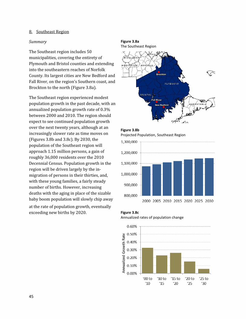
45
8. Southeast Region
Summary
The Southeast region includes 50
municipalities, covering the entirety of
Plymouth and Bristol counties and extending
into the southeastern reaches of Norfolk
County. Its largest cities are New Bedford and
Fall River, on the region’s Southern coast, and
Brockton to the north (Figure 3.8a).
The Southeast region experienced modest
population growth in the past decade, with an
annualized population growth rate of 0.3%
between 2000 and 2010. The region should
expect to see continued population growth
over the next twenty years, although at an
increasingly slower rate as time moves on
(Figures 3.8b and 3.8c). By 2030, the
population of the Southeast region will
approach 1.15 million persons, a gain of
roughly 36,000 residents over the 2010
Decennial Census. Population growth in the
region will be driven largely by the in-
migration of persons in their thirties, and,
with these young families, a fairly steady
number of births. However, increasing
deaths with the aging in place of the sizable
baby boom population will slowly chip away
at the rate of population growth, eventually
exceeding new births by 2020.
Figure 3.8a The Southeast Region
Figure 3.8c Annualized rates of population change
Figure 3.8b Projected Population, Southeast Region
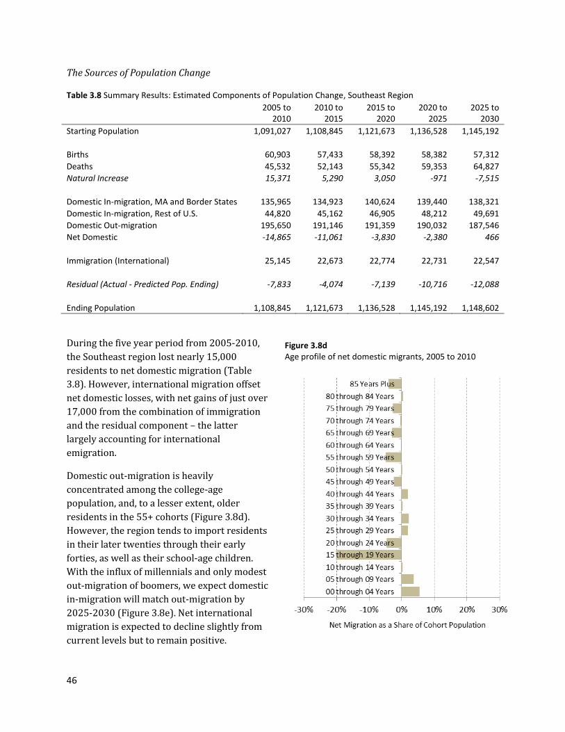
46
The Sources of Population Change
Table 3.8 Summary Results: Estimated Components of Population Change, Southeast Region
2005 to
2010 2010 to
2015 2015 to
2020 2020 to
2025 2025 to
2030
Starting Population 1,091,027 1,108,845 1,121,673 1,136,528 1,145,192
Births 60,903 57,433 58,392 58,382 57,312
Deaths 45,532 52,143 55,342 59,353 64,827
Natural Increase 15,371 5,290 3,050 -971 -7,515
Domestic In-migration, MA and Border States 135,965 134,923 140,624 139,440 138,321
Domestic In-migration, Rest of U.S. 44,820 45,162 46,905 48,212 49,691
Domestic Out-migration 195,650 191,146 191,359 190,032 187,546
Net Domestic -14,865 -11,061 -3,830 -2,380 466
Immigration (International) 25,145 22,673 22,774 22,731 22,547
Residual (Actual - Predicted Pop. Ending) -7,833 -4,074 -7,139 -10,716 -12,088
Ending Population 1,108,845 1,121,673 1,136,528 1,145,192 1,148,602
During the five year period from 2005-2010,
the Southeast region lost nearly 15,000
residents to net domestic migration (Table
3.8). However, international migration offset
net domestic losses, with net gains of just over
17,000 from the combination of immigration
and the residual component – the latter
largely accounting for international
emigration.
Domestic out-migration is heavily
concentrated among the college-age
population, and, to a lesser extent, older
residents in the 55+ cohorts (Figure 3.8d).
However, the region tends to import residents
in their later twenties through their early
forties, as well as their school-age children.
With the influx of millennials and only modest
out-migration of boomers, we expect domestic
in-migration will match out-migration by
2025-2030 (Figure 3.8e). Net international
migration is expected to decline slightly from
current levels but to remain positive.
Figure 3.8d Age profile of net domestic migrants, 2005 to 2010
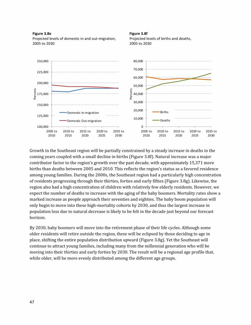
47
Growth in the Southeast region will be partially constrained by a steady increase in deaths in the
coming years coupled with a small decline in births (Figure 3.8f). Natural increase was a major
contributor factor to the region’s growth over the past decade, with approximately 15,371 more
births than deaths between 2005 and 2010. This reflects the region’s status as a favored residence
among young families. During the 2000s, the Southeast region had a particularly high concentration
of residents progressing through their thirties, forties and early fifties (Figure 3.8g). Likewise, the
region also had a high concentration of children with relatively few elderly residents. However, we
expect the number of deaths to increase with the aging of the baby boomers. Mortality rates show a
marked increase as people approach their seventies and eighties. The baby boom population will
only begin to move into these high-mortality cohorts by 2030, and thus the largest increase in
population loss due to natural decrease is likely to be felt in the decade just beyond our forecast
horizon.
By 2030, baby boomers will move into the retirement phase of their life cycles. Although some
older residents will retire outside the region, these will be eclipsed by those deciding to age in
place, shifting the entire population distribution upward (Figure 3.8g). Yet the Southeast will
continue to attract young families, including many from the millennial generation who will be
moving into their thirties and early forties by 2030. The result will be a regional age profile that,
while older, will be more evenly distributed among the different age groups.
100,000
125,000
150,000
175,000
200,000
225,000
250,000
2005 to2010
2010 to2015
2015 to2020
2020 to2025
2025 to2030
Per
son
s
Domestic In-migration
Domestic Out-migration
0
10,000
20,000
30,000
40,000
50,000
60,000
70,000
80,000
2005 to2010
2010 to2015
2015 to2020
2020 to2025
2025 to2030
Per
son
s
Births
Deaths
Figure 3.8e Projected levels of domestic in and out-migration, 2005 to 2030
Figure 3.8f Projected levels of births and deaths, 2005 to 2030
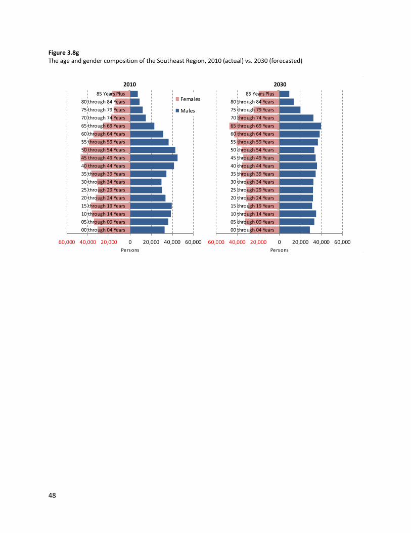
48
60,000 40,000 20,000 0 20,000 40,000 60,000
00 through 04 Years
05 through 09 Years
10 through 14 Years
15 through 19 Years
20 through 24 Years
25 through 29 Years
30 through 34 Years
35 through 39 Years
40 through 44 Years
45 through 49 Years
50 through 54 Years
55 through 59 Years
60 through 64 Years
65 through 69 Years
70 through 74 Years
75 through 79 Years
80 through 84 Years
85 Years Plus
Persons
Females
Males
60,000 40,000 20,000 0 20,000 40,000 60,000
00 through 04 Years
05 through 09 Years
10 through 14 Years
15 through 19 Years
20 through 24 Years
25 through 29 Years
30 through 34 Years
35 through 39 Years
40 through 44 Years
45 through 49 Years
50 through 54 Years
55 through 59 Years
60 through 64 Years
65 through 69 Years
70 through 74 Years
75 through 79 Years
80 through 84 Years
85 Years Plus
Persons
2010 2030
Figure 3.8g The age and gender composition of the Southeast Region, 2010 (actual) vs. 2030 (forecasted)
49
IV. Technical Discussion of Methods and Assumptions
This section provides a technical description of the process used to develop the 1) regional and 2)
municipal-level population projections using a cohort component approach. While both levels of
projections are prepared using a cohort component method, the major methodological difference is
in the way migration is modeled: the municipal-level estimates (also referred to as Minor Civil
Divisions, or MCDs) rely on residual net migration rates computed from vital statistics, while the
sub-state regional projections use gross domestic migration rates based on the American
Community Survey Public Use Microdata (ACS PUMS). MCD projections are controlled to the eight
regions’ projections in order to smooth out variations due to data quality issues at the MCD level
and ensure more consistent and accurate projections at higher-level geographies. These controlled
MCD projections can then be re-aggregated to other areas of interest, such as counties, regional
planning areas, etc.
A. Regional-Level Methods and Assumptions
Summary
This section describes the process and data used to develop the regional population projections.
These projections were developed separately for eight regions, although each region was produced
following a generally similar framework. The methodology describing how the regional projections
were used to estimate municipal population projections follows in Part B of this section.
Our regional projections are based on a demographic accounting framework for modeling
population change, commonly referred to as a cohort-component model. The cohort-component
method recognizes that there are only four ways that a region’s population can change from one
time period to the next. It can add residents through either births or in-migration, or it can lose
residents through deaths or out-migration. We further divide migration by whether domestic or
international, and use separate estimation methods for each.
The cohort-component approach also accounts for population change associated with the aging of
the population. The current age profile is a strong predictor of future population levels, growth and
decline. The age profile of the population can differ greatly from one region to another. For
example, the Greater Boston region has a high concentration of residents in their twenties and early
thirties, while the Cape and Islands have large shares of near and post-retirement age residents.
Furthermore, the likelihood of birth, death, and in- and out-migration all vary by age. Because
fertility rates are highest among women in their twenties and early thirties, a place that is
anticipating a large number of women coming into their twenties and thirties in the next decade
will likely experience more births. Similarly, mortality rates are notably higher for persons seventy
years and older, such that an area with a large concentration of elderly residents will experience
more deaths in decades to come.
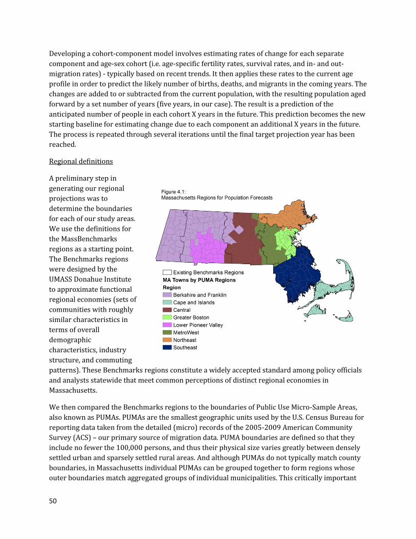
50
Developing a cohort-component model involves estimating rates of change for each separate
component and age-sex cohort (i.e. age-specific fertility rates, survival rates, and in- and out-
migration rates) - typically based on recent trends. It then applies these rates to the current age
profile in order to predict the likely number of births, deaths, and migrants in the coming years. The
changes are added to or subtracted from the current population, with the resulting population aged
forward by a set number of years (five years, in our case). The result is a prediction of the
anticipated number of people in each cohort X years in the future. This prediction becomes the new
starting baseline for estimating change due to each component an additional X years in the future.
The process is repeated through several iterations until the final target projection year has been
reached.
Regional definitions
A preliminary step in
generating our regional
projections was to
determine the boundaries
for each of our study areas.
We use the definitions for
the MassBenchmarks
regions as a starting point.
The Benchmarks regions
were designed by the
UMASS Donahue Institute
to approximate functional
regional economies (sets of
communities with roughly
similar characteristics in
terms of overall
demographic
characteristics, industry
structure, and commuting
patterns). These Benchmarks regions constitute a widely accepted standard among policy officials
and analysts statewide that meet common perceptions of distinct regional economies in
Massachusetts.
We then compared the Benchmarks regions to the boundaries of Public Use Micro-Sample Areas,
also known as PUMAs. PUMAs are the smallest geographic units used by the U.S. Census Bureau for
reporting data taken from the detailed (micro) records of the 2005-2009 American Community
Survey (ACS) – our primary source of migration data. PUMA boundaries are defined so that they
include no fewer the 100,000 persons, and thus their physical size varies greatly between densely
settled urban and sparsely settled rural areas. And although PUMAs do not typically match county
boundaries, in Massachusetts individual PUMAs can be grouped together to form regions whose
outer boundaries match aggregated groups of individual municipalities. This critically important
51
feature allows us to match Census micro-data with other Census data and State vital statistics
estimates we obtained at the municipal level (i.e. births and deaths). We performed our regional
grouping using Geographic Information System mapping software. The resulting study regions are
presented in Figure 4.1.
Estimating the components of change
Determining the launch year and cohort classes
We begin by classifying the composition of resident population into discrete cohorts by age and sex.
Following standard practice, we use five year age cohorts (e.g. 0 to 4 years old, 5 to 9,… 80 to 84,
and 85 or older) and develop separate profiles for males and females, based on information
provided in the 100% Count (SF 1) file of the 2010 Decennial Census of Population. This will also
serve as the starting point (i.e. launch year) for generating forecasts.
Deaths and Survival
The first component of change is survival. Our projections require an estimate of the number of
people in the current population who are expected to live an additional five years into the future.
Estimating the survival rate of each cohort is fairly straightforward. The Massachusetts Department
of Public Health provided us with a detailed dataset that included all known deaths in the
Commonwealth that occurred between 2000 to the end of calendar year 2009. This database
includes information on the sex, age, and place of residence of the deceased, which we aggregated
into our study regions by age/sex cohort. We estimate the five year survival rate for each cohort (j)
in study region (i) as one minus the average number of deaths over the past five years (2005 to
2009) divided by the base population in 2005 and then raised to the fifth power, or:
[ (
)]
. (1)
Following the recommendations of Isserman (1993), we calculate an operational survival rate as
the average of the five year survival rates across successive age cohorts. The operational rate
recognizes that, over the next five years, the average person will spend half their time in their
current age cohort and half their time in the next cohort. We estimate the number of eventual
survivors in each cohort by 2015 by multiplying the operational survival rate against the cohort
population count as reported by the 2010 Census.
Domestic Migration
Migration is the most dynamic component of change, and often makes the difference between
whether a region shows swift growth, relative stability, or gradual decline. Migration is also the
most difficult component to estimate and is the most likely source of uncertainty and error in
population projections. Whereas fertility and mortality follow fairly regular age-related patterns,
the migration behavior of similar age groups is influenced by regional and national differences in
socio-economic conditions. Furthermore, the data needed to estimate migration is often restricted

52
or limited, especially for many small areas. Even when it is available, it is based on statistical
samples and not actual population counts, and thus is prone to sampling error – which will be
larger for smaller regions.
Due to data limitations and the other methodological challenges, applied demographers have
developed a variety of alternate models and methods to estimate migration rates. No single method
works best in all circumstances, and we evaluated numerous approaches in the development of our
projections. Those presented in this report are based on a particularly novel approach known as a
multi-region gross migration model as discussed by Isserman (1993); Smith, Tayman and Swanson
(2001); and Renski and Strate. Most analysts use a net-migration approach, where a single net
migration rate is calculated as the number of net new migrants per cohort (in-migrants minus out-
migrants) divided by the baseline cohort population of the study region. Although common, the net
migration approach suffers from several conceptual and empirical flaws. A major problem is that
denominator of the net migration rate is based purely on the number of residents in the study
region. However, none of the existing residents are at risk of migrating into the region – they
already live there. While this may seem trivial, it has been shown to lead to erroneous and biased
projections especially for fast growing and declining regions.
A gross-migration approach calculates separate rates for in- and out-migrants. Beyond generating
more accurate forecasts in most cases, it has an added benefit in that it connects regional
population change to broader regional and national forces – rather than simply treating any one
region as an isolated area. This type of model is made possible by utilizing the rich detail of
information available through the newly released Public Use Micro-Samples (PUMS) of American
Community Survey (ACS). The ACS is a relatively new data product of the U.S. Census Bureau that
replaced the detailed information collected on the long-form of the decennial census (STF 3). It asks
residents questions about where they lived one year prior, which can be used to estimate the
number of domestic in- and out migrants. Unfortunately, the ACS does not report enough detail to
estimate migration rates by detailed age-sex cohorts in its standard products. This information can
be tabulated from the ACS PUMS – which is 5% random sample of individual records taken drawn
the ACS surveys. Each record in the PUMS is given a survey weight, which we use to estimate the
total number of migrants by detailed age and sex cohorts. It is very important to realize that the
PUMS records are based on small, although representative, samples – and that the smaller the
sample the greater the margin of error. Sample sizes can be particularly small when distributed by
age and sex cohorts for different types of migrants, especially in small regions.
Estimating domestic out-migration is largely similar to estimating net-migration. Because current
residents of the study region (i) are those who are ‘at risk’ of moving out, so the appropriate cohort
(j) migration rate is:
(
). (2)
Because migration in the ACS is based on place of residence one year prior, the out-migration rate
reported in equation (2) is the equivalent of a single year rate. We multiply this by five to estimate
the five-year equivalent rate, and, as we did with survival rates, average the five year rates across
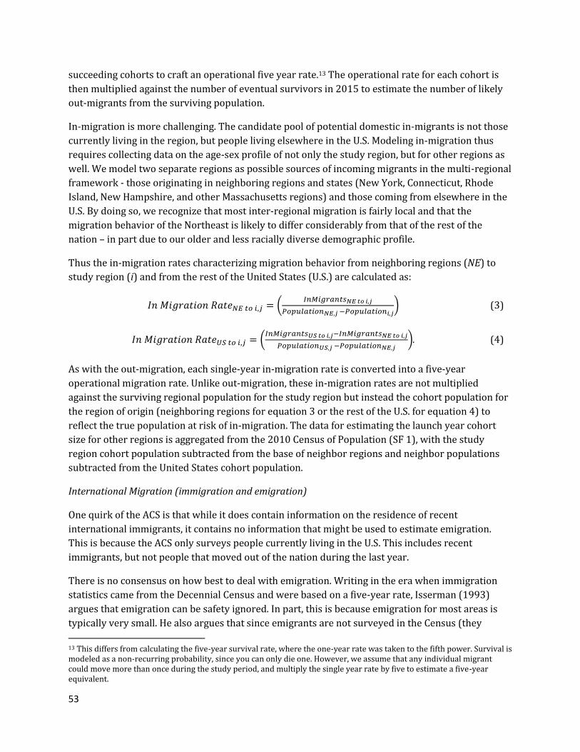
53
succeeding cohorts to craft an operational five year rate.13 The operational rate for each cohort is
then multiplied against the number of eventual survivors in 2015 to estimate the number of likely
out-migrants from the surviving population.
In-migration is more challenging. The candidate pool of potential domestic in-migrants is not those
currently living in the region, but people living elsewhere in the U.S. Modeling in-migration thus
requires collecting data on the age-sex profile of not only the study region, but for other regions as
well. We model two separate regions as possible sources of incoming migrants in the multi-regional
framework - those originating in neighboring regions and states (New York, Connecticut, Rhode
Island, New Hampshire, and other Massachusetts regions) and those coming from elsewhere in the
U.S. By doing so, we recognize that most inter-regional migration is fairly local and that the
migration behavior of the Northeast is likely to differ considerably from that of the rest of the
nation – in part due to our older and less racially diverse demographic profile.
Thus the in-migration rates characterizing migration behavior from neighboring regions (NE) to
study region (i) and from the rest of the United States (U.S.) are calculated as:
(
) (3)
(
). (4)
As with the out-migration, each single-year in-migration rate is converted into a five-year
operational migration rate. Unlike out-migration, these in-migration rates are not multiplied
against the surviving regional population for the study region but instead the cohort population for
the region of origin (neighboring regions for equation 3 or the rest of the U.S. for equation 4) to
reflect the true population at risk of in-migration. The data for estimating the launch year cohort
size for other regions is aggregated from the 2010 Census of Population (SF 1), with the study
region cohort population subtracted from the base of neighbor regions and neighbor populations
subtracted from the United States cohort population.
International Migration (immigration and emigration)
One quirk of the ACS is that while it does contain information on the residence of recent
international immigrants, it contains no information that might be used to estimate emigration.
This is because the ACS only surveys people currently living in the U.S. This includes recent
immigrants, but not people that moved out of the nation during the last year.
There is no consensus on how best to deal with emigration. Writing in the era when immigration
statistics came from the Decennial Census and were based on a five-year rate, Isserman (1993)
argues that emigration can be safety ignored. In part, this is because emigration for most areas is
typically very small. He also argues that since emigrants are not surveyed in the Census (they
13 This differs from calculating the five-year survival rate, where the one-year rate was taken to the fifth power. Survival is modeled as a non-recurring probability, since you can only die one. However, we assume that any individual migrant could move more than once during the study period, and multiply the single year rate by five to estimate a five-year equivalent.
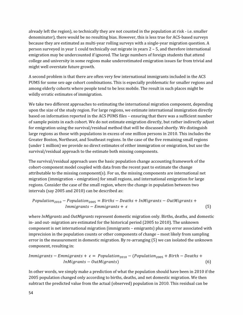
54
already left the region), so technically they are not counted in the population at risk - i.e. smaller
denominator), there would be no resulting bias. However, this is less true for ACS-based surveys
because they are estimated as multi-year rolling surveys with a single-year migration question. A
person surveyed in year 1 could technically out migrate in years 2 – 5, and therefore international
emigration may be undercounted if ignored. The large numbers of foreign students that attend
college and university in some regions make underestimated emigration issues far from trivial and
might well overstate future growth.
A second problem is that there are often very few international immigrants included in the ACS
PUMS for some sex-age cohort combinations. This is especially problematic for smaller regions and
among elderly cohorts where people tend to be less mobile. The result in such places might be
wildly erratic estimates of immigration.
We take two different approaches to estimating the international migration component, depending
upon the size of the study region. For large regions, we estimate international immigration directly
based on information reported in the ACS PUMS files – ensuring that there was a sufficient number
of sample points in each cohort. We do not estimate emigration directly, but rather indirectly adjust
for emigration using the survival/residual method that will be discussed shortly. We distinguish
large regions as those with populations in excess of one million persons in 2010. This includes the
Greater Boston, Northeast, and Southeast regions. In the case of the five remaining small regions
(under 1 million) we provide no direct estimates of either immigration or emigration, but use the
survival/residual approach to the estimate both missing components.
The survival/residual approach uses the basic population change accounting framework of the
cohort-component model coupled with data from the recent past to estimate the change
attributable to the missing component(s). For us, the missing components are international net
migration (immigration – emigration) for small regions, and international emigration for large
regions. Consider the case of the small region, where the change in population between two
intervals (say 2005 and 2010) can be described as:
(5)
where InMigrants and OutMigrants represent domestic migration only. Births, deaths, and domestic
in- and out- migration are estimated for the historical period (2005 to 2010). The unknown
component is net international migration (immigrants – emigrants) plus any error associated with
imprecision in the population counts or other components of change – most likely from sampling
error in the measurement in domestic migration. By re-arranging (5) we can isolated the unknown
component, resulting in:
(6)
In other words, we simply make a prediction of what the population should have been in 2010 if the
2005 population changed only according to births, deaths, and net domestic migration. We then
subtract the predicted value from the actual (observed) population in 2010. This residual can be
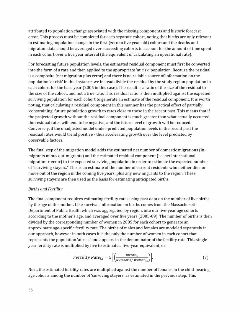
55
attributed to population change associated with the missing components and historic forecast
error. This process must be completed for each separate cohort, noting that births are only relevant
to estimating population change in the first (zero to five year-old) cohort and the deaths and
migration data should be averaged over succeeding cohorts to account for the amount of time spent
in each cohort over a five year interval (the equivalent of calculating an operational rate).
For forecasting future population levels, the estimated residual component must first be converted
into the form of a rate and then applied to the appropriate ‘at risk’ population. Because the residual
is a composite (net migration plus error) and there is no reliable source of information on the
population ‘at risk’ in this instance, we instead divide the residual by the study region population in
each cohort for the base year (2005 in this case). The result is a ratio of the size of the residual to
the size of the cohort, and not a true rate. This residual ratio is then multiplied against the expected
surviving population for each cohort to generate an estimate of the residual component. It is worth
noting, that calculating a residual component in this manner has the practical effect of partially
‘constraining’ future population growth to rates close to those in the recent past. This means that if
the projected growth without the residual component is much greater than what actually occurred,
the residual rates will tend to be negative, and the future level of growth will be reduced.
Conversely, if the unadjusted model under-predicted population levels in the recent past the
residual rates would trend positive - thus accelerating growth over the level predicted by
observable factors.
The final step of the migration model adds the estimated net number of domestic migrations (in-
migrants minus out-migrants) and the estimated residual component (i.e. net international
migration + error) to the expected surviving population in order to estimate the expected number
of “surviving stayers.” This is an estimate of the number of current residents who neither die nor
move out of the region in the coming five years, plus any new migrants to the region. These
surviving stayers are then used as the basis for estimating anticipated births.
Births and Fertility
The final component requires estimating fertility rates using past data on the number of live births
by the age of the mother. Like survival, information on births comes from the Massachusetts
Department of Public Health which was aggregated, by region, into our five-year age cohorts
according to the mother’s age, and averaged over five years (2005-09). The number of births is then
divided by the corresponding number of women in 2005 for each cohort to generate an
approximate age-specific fertility rate. The births of males and females are modeled separately in
our approach, however in both cases it is the only the number of women in each cohort that
represents the population ‘at risk’ and appears in the denominator of the fertility rate. This single
year fertility rate is multiplied by five to estimate a five-year equivalent, or:
[(
)]. (7)
Next, the estimated fertility rates are multiplied against the number of females in the child-bearing
age cohorts among the number of ‘surviving stayers’ as estimated in the previous step. This
56
provides an estimate of the number of babies that are anticipated within the next five years, and
this number is summed across all maternal age cohorts.
Aging the population and generating projections for later years
The final step in generating our first set of five year forecasts (for year 2015) is to age the surviving
stayers in all cohorts by five years. The first (0 to 4) and final (85+) cohorts are treated differently.
The number of anticipated babies estimated in the previous step becomes the number of 0 to 4 year
olds in 2015. The number of persons in the 85+ cohort in 2015 is the number of surviving stayers in
the 80 to 84 age cohort (in 2010) added to the number of surviving stayers in the 85 and older
cohort. As we made separate estimated for males and females the two populations are added and
summed across all cohorts to determine the projected number of residents in 2015.
This process is essentially repeated for all future year projections, except that the rates developed
from historic data remain the same throughout the forecast horizon. Our 2015 projection becomes
our launch year population for estimating the 2020 population, which in turn is used to seed the
2025 population and so-forth. The only notable difference in the process used to generate the later
year forecasts is the need to have outside projections of future population levels for the nation as a
whole and for neighboring states. This is necessary for estimated the population ‘at-risk’ of
domestic in-migrants. The U.S. Census Bureau regularly generates highly detailed national
population forecasts.14 We use the latest release of national forecasts (release date May, 2013)
which are based on information from the 2010 Decennial Census. Unfortunately, the Census Bureau
no longer generates detailed state-level long-term projections. Lacking a better source, we use the
final set of Census-based state projections (release date 2005) for estimating future in-migrants
from neighboring states. In future updates, we hope to either develop or acquire more updated
state-level projections.
14 http://www.census.gov/population/projections/
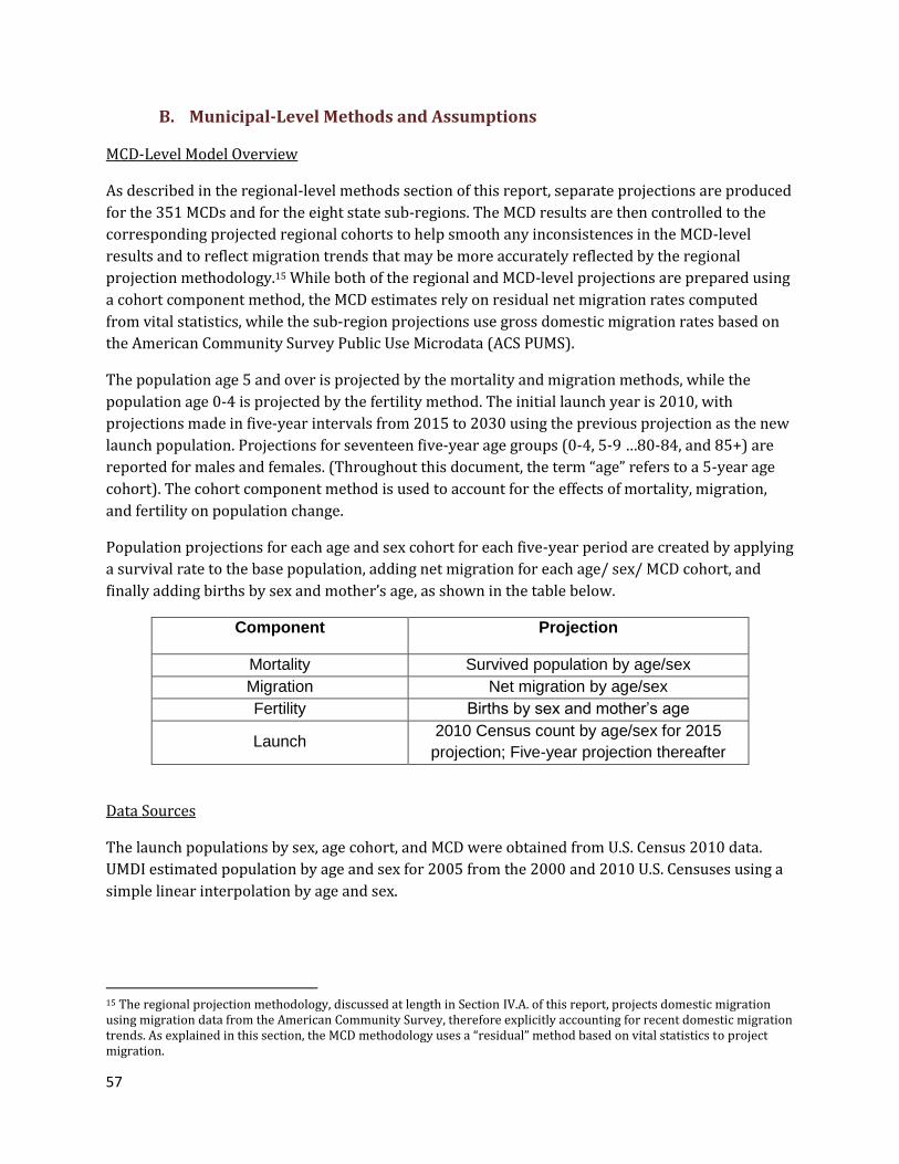
57
B. Municipal-Level Methods and Assumptions
MCD-Level Model Overview
As described in the regional-level methods section of this report, separate projections are produced
for the 351 MCDs and for the eight state sub-regions. The MCD results are then controlled to the
corresponding projected regional cohorts to help smooth any inconsistences in the MCD-level
results and to reflect migration trends that may be more accurately reflected by the regional
projection methodology.15 While both of the regional and MCD-level projections are prepared using
a cohort component method, the MCD estimates rely on residual net migration rates computed
from vital statistics, while the sub-region projections use gross domestic migration rates based on
the American Community Survey Public Use Microdata (ACS PUMS).
The population age 5 and over is projected by the mortality and migration methods, while the
population age 0-4 is projected by the fertility method. The initial launch year is 2010, with
projections made in five-year intervals from 2015 to 2030 using the previous projection as the new
launch population. Projections for seventeen five-year age groups (0-4, 5-9 …80-84, and 85+) are
reported for males and females. (Throughout this document, the term “age” refers to a 5-year age
cohort). The cohort component method is used to account for the effects of mortality, migration,
and fertility on population change.
Population projections for each age and sex cohort for each five-year period are created by applying
a survival rate to the base population, adding net migration for each age/ sex/ MCD cohort, and
finally adding births by sex and mother’s age, as shown in the table below.
Component Projection
Mortality Survived population by age/sex
Migration Net migration by age/sex
Fertility Births by sex and mother’s age
Launch 2010 Census count by age/sex for 2015
projection; Five-year projection thereafter
Data Sources
The launch populations by sex, age cohort, and MCD were obtained from U.S. Census 2010 data.
UMDI estimated population by age and sex for 2005 from the 2000 and 2010 U.S. Censuses using a
simple linear interpolation by age and sex.
15 The regional projection methodology, discussed at length in Section IV.A. of this report, projects domestic migration using migration data from the American Community Survey, therefore explicitly accounting for recent domestic migration trends. As explained in this section, the MCD methodology uses a “residual” method based on vital statistics to project migration.
58
UMDI requested and received confidential vital statistics data for births and deaths from January 1,
2000 through December 31, 2009 from the Massachusetts Department of Public Health. From
these, UMDI estimated survival, birth and residual net migration rates.
MCD Projections Launch Population
Initial Launch Population
The initial launch population for the 2015 projection is the 2010 Census population by age/sex for
each MCD. Corrected census counts from the Count Question Resolution (CQR) program are
incorporated where applicable. Each projection thereafter uses the previous projection as the
launch population (i.e. the 2020 projection uses the 2015 projection as the launch population).
MCD Projections: Mortality
Forward Cohort Survival Method
The forward cohort survival method is used to account for the mortality component of population
change. This procedure applies five-year survival rates by age/sex to the launch population by
age/sex for MCDs in order to survive their populations out five years, resulting in the expected
population age five and over before accounting for migration.
5-Year Survival Rates by Age/Sex
UMDI calculated five-year survival rates by age and sex using deaths by age, sex and MCD from
2000 to 2009 (January 1, 2000 through December 31, 2009). Survival rates by age, sex and MCD
were assumed to be constant for the duration of the projections (from 2010 through 2030).
Survival rates for each age cohort up to 80-84 were averaged with the next-older cohort to account
for the fact that roughly half of each cohort would age into the next cohort over the course of each
5-year period. The 85+ cohort’s survival rate was used as-is, since there was no older cohort to
average.
MCDs with smaller populations demonstrated a degree of variability in survival rates that we
considered too broad for optimal results. Therefore, for MCDs with populations lower than 10,000
as of the 2000 Census, we used regional survival rates by age and sex instead of MCD-specific rates
to smooth the results. We calculated regional rates using the same MCD-based vital statistics data
from 2000-2009 as we used in calculating the MCD rates.
Survived Population for MCDs
The base population by age/sex for MCDs is survived to the next 5-year projection by applying the
corresponding averaged five-year survival rates by age/sex.
Lag in Death Data
For each current vintage, vital statistics data showing deaths will only be available for past years –
for instance, in producing the Vintage 2013 estimates (the first vintage), we have death data only
through 2009.
59
Key Assumptions
The methodology assumes that survival rates vary most significantly by age and sex. To some
extent, the use of MCD-specific rates will also indirectly account for varying socioeconomic factors,
including race and ethnicity, which vary by MCD and may affect survival rates. The methodology
assumes that survival rates by age, sex and MCD will stay constant over the next 20 years.
MCD Projections: Migration
Residual Net Migration from Vital Statistics
The residual net migration method is used to account for the migration component of population
change. “Residual” refers to the fact that migration is assumed to be responsible for past population
change after accounting for births and deaths. This residual net migration is then used to estimate
past migration rates. The procedure applies the resulting net migration rates by age/sex estimated
for each MCD to the MCD’s survived population by age/sex in order to project net migration by
age/sex for the population age 5 and over. For the population ages 0-4, it is assumed that residence
of infants will be determined by the migration of their birth mothers. For MCDs with 2000 Census
population below 10,000, a linear migration assumption (described below) is used to smooth
migration.
Determination of Net Migration Rates
Vital statistics are used to infer net migration totals for 2000-2009. In order to calculate five-year
net migration by age, sex and MCD, natural increase (births minus deaths) by age/ sex for 2000-
2005 is added to the 2000 population by age/ sex for each MCD, and then the results are subtracted
from the interpolated 2005 population by age/ sex for each MCD to estimate net migration by age/
sex and MCD for 2000-2005. A similar process calculates migration between 2005 and 2010.
For MCDs with 2000 population equal to or greater 10,000, the two five-year net migration
estimates are averaged and rates are then calculated for each age, sex and MCD. The resulting rates
are applied to the base population to project five-year net migration. The resulting average five-
year net migration rates by age/sex are held constant throughout the projection period.
For MCDs with 2000 population under 10,000, five-year net migration by age, sex and MCD is held
constant, and population cohorts are never allowed to go below zero. This avoids applying
unrealistically high migration rates to small populations. For instance, if an MCD starts with 4 males
aged 70-74 and net migration shows 4 more move in over five years, the result is a migration rate
of 2. This results in highly variable and unrealistic results in some cases. . In this example, holding
migration linear means that in each five-year projection period, four males aged 70-74 will move
into the MCD. UMDI conducted sensitivity testing for this method and found that the model with
constant migration for small places in most cases resulted in more realistic, gradual population
growth or decline, as well as more realistic sex and age profiles for these MCDs.
60
Key Assumptions
The use of a net migration rate relies on a base for migration that includes only current residents –
in other words, only those at risk of out-migration. Nonresidents who are at risk of in-migration are
not explicitly accounted for in the MCD method, and this results in some inaccuracy which is
minimized by the process of controlling to regional total projections that are based on a gross
migration model.
We assume that age, sex and MCD are the key factors by which migration rates vary. Other factors,
including non-demographic factors such as macroeconomic factors, or local policy changes, are not
explicitly included in this model. Future projections models may incorporate these or other factors.
Fertility
Vital Statistics Method
We apply age-specific fertility rates to the migrated female population by age to project births by
age of mother, followed by survival rates for the population aged 0-4. Total survived births are then
derived by summing across all maternal age groups, and the results represent the projected
population age 0-4. For each MCD, the number of males and females is assumed to be the same as
the proportion of male or female births statewide.
Fertility by Age of Mother
Average births by age of mother for each MCD are calculated for two five-year periods (2000-2005
and 2005-2010) using nine maternal age groups, from 10-14…50-54.
Fertility Rates
Age-specific fertility rates are computed for each time period by dividing the average number of
births by age of mother by the corresponding number of females of that age group. The average
age-specific fertility rates are held constant throughout the projection period. The base population
for launching a new five-year projection is the survived, post-migration projected female
population by age.
MCDs with smaller populations demonstrated a degree of variability in fertility rates that we
considered too broad for optimal results. Therefore, for MCDs with populations lower than 10,000
as of the 2000 Census, we used regional fertility rates by age and sex instead of MCD-specific rates
to smooth the results. We calculated regional rates using the same MCD-based vital statistics data
from 2000-2009 as we used in calculating the MCD rates.
Lag in Birth Data
For each current vintage, birth data will only be available for past years – for instance, in producing
the Vintage 2013 estimates (the first vintage), we have birth data only through 2009.
61
Key Assumptions
We assume age, sex and MCD to be adequate indicators of fertility rates for MCD for the first vintage
projections. We assume that the proportion of male to female births does not vary significantly by
geography or maternal age. We assume that fertility rates by maternal age and MCD will not change
significantly over time. Future iterations of the projections may amend these assumptions based on
available data.
Controlling to the Regional-level Projections
The resulting MCD-level projected cohorts are finally controlled to the regional-level projected
cohorts. To do this, we assume that each MCD’s share of the region’s population, for each age and
sex cohort, is given by the MCD population projections. Those shares are then applied to the
regional projections to arrive at adjusted age/ sex cohorts for each MCD.
62
Sources:
Isserman, A. M. (1993). "The Right People, The Right Rates - Making Population Estimates with an
Interregional Cohort-Component Model." Journal of the American Planning Association 59(1): 45-
64.
Renski, H.C. and S. Strate. 2013. “Evaluating the migration component of county-level population
estimates.” Journal of Planning Education and Research. 33(3), 325-335.
Smith, S., J. Tayman and D. Swanson. (2001) State and Local Population Projections: Methodology
and Analysis. New York: Kluwer Academic. Ch. 3- 7

63
Appendix A
UMass Donahue Institute Population Projections Advisory Committee Joseph Buckley Massachusetts School Building Authority Bradley Egan Project Manager Massachusetts School Building Authority Dr. Alan Clayton Matthews Professor and Director of Quantitative Methods Northeastern University Saul Franklin Consultant / Former Director of MassChip Massachusetts Department of Public Health Molly Goren-Watts Principal Planner/Manager Pioneer Valley Planning Commission Marilyn McCrory, AICP Water Resources Planner, Office of Water Resources Massachusetts Dept. of Conservation & Recreation Dr. James West Senior Demographer/Epidemiologist Massachusetts Department of Public Health Dr. Stefan Rayer Research Demographer, Bureau of Economic & Business Research University of Florida Federal-State Cooperative for Population Projections Member Timothy Reardon Manager of Planning Research Metropolitan Area Planning Council Jennifer Song State Demographer North Carolina Office of State Budget and Management Federal-State Cooperative for Population Projections Member Jan K. Vink Research Support Specialist, Program on Applied Demographics Cornell University Chair, Federal State Cooperative for Population Projections
Related Documents