Long-Run Inflation Risk and the Postwar Term Premium

Long-Run In�ation Risk and thePostwar Term Premium�

Glenn D. Rudebuschy Eric T. Swansonz

February 2008

AbstractLong-term bond yields in the U.S. steadily rose during the 1960s and 1970s and

then retreated over the next two decades. This rise and fall is di¢ cult to explain us-ing only changes in long-term in�ation expectations and real interest rates; instead,an additional role for changes in the term premium� the risk premium on long-termbonds� appears to be required. We explain the behavior of long-term bond yields witha New Keynesian DSGE model with nominal rigidities, Epstein-Zin-Weil preferences,and long-run in�ation risk. We show that this model� unlike many others� is able togenerate an empirically plausible level of the term premium without compromising themodel�s ability to �t key macroeconomic variables. Moreover, by taking into accountchanges in the Federal Reserve�s perceived commitment to a low long-term U.S. in�a-tion rate, the model�s predictions for in�ation expectations and the term premium areable to explain the behavior of U.S. long-term bond yields in the postwar period.

�The views expressed in this paper are those of the authors and do not necessarily re�ect the views ofother individuals within the Federal Reserve System.

yFederal Reserve Bank of San Francisco; http://www.frbsf.org/economists/grudebusch; [email protected].

zFederal Reserve Bank of San Francisco; http://www.ericswanson.us; [email protected].

1 Introduction

From 1955 to 1981, the nominal yield on the 10-year U.S. Treasury bond more than quin-

tupled, rising steadily from 2.6 percent at the beginning of this period to over 15.3 percent

by the end. From 1982 to 2008, the 10-year bond yield then reversed course, falling all the

way back to 3.7 percent (see Figure 1). It is di¢ cult to explain these dramatic changes in

long-term bond yields solely as a result of changes in long-run in�ation expectations or real

interest rates. For example, Figure 2 plots survey data on long-term in�ation expectations

starting in 1980 (the date this question was �rst included in the survey). This measure of

long-run in�ation expectations peaked at about 8.25 percent in late 1980, and then declined

steadily to about 2.5 percent. Although this fall is substantial, it can account for only about

half of the decline in the long-term nominal bond yield over the same period. Similarly, it

appears unlikely that elevated long-term real interest rates could account for the high nom-

inal rates of the 1970s and 1980s: indeed, given the well-known period of slow productivity

growth from the mid-1970s through the mid-1990s, it seems likely that equilibrium real in-

terest rates were, if anything, lower during this period rather than higher. Finally, there is

a large �nance literature that argues that risk premia on long-term bonds are substantial

and vary signi�cantly over time (e.g., Fama and Bliss, 1987, Campbell and Shiller, 1991,

Cochrane and Piazessi, 2005). Thus, one is naturally led to wonder whether and to what

extent variation in the term premium over the postwar period may have been responsible

for the rise and fall of long-term bond yields.

In the present paper, we develop a dynamic structural general equilibrium (DSGE) model

of the U.S. economy that is able to account for the dynamics of macroeconomic variables,

changes in long-term in�ation expectations, and changes in the risk premium on long-term

bonds. To do this, our model requires three essential ingredients. First, as in Christiano,

Eichenbaum, and Evans (2005), Smets and Wouters (2003), and others, we require an impor-

tant role for nominal rigidities in order to match the behavior of in�ation and other nominal

quantities. Without nominal rigidities, we would have little hope of matching the variation

in the returns on nominal bonds.

1

10­year U.S. Treasury Yield

0

2

4

6

8

10

12

14

16

1955

1957

1959

1961

1963

1965

1967

1969

1971

1973

1975

1977

1979

1981

1983

1985

1987

1989

1991

1993

1995

1997

1999

2001

2003

2005

2007

Figure 1: Constant-maturity 10-year U.S. Treasury note yield. Source: Federal Reserve Board, H.15

release, monthly average yield.

Long­Term Inflation Expectations

0

1

2

3

4

5

6

7

8

9

1980

1982

1983

1985

1986

1988

1989

1990

1991

1992

1993

1993

1994

1995

1996

1996

1997

1998

1999

1999

2000

2001

2002

2002

2003

2004

2005

2005

2006

2007

Figure 2: Long-term in�ation expectations of survey respondents (in�ation expectations from 5 to 10 years

ahead). Source: Blue Chip, semiannual frequency. Survey question �rst asked in 1980.

2

Second, in order to generate a nontrivial term premium, we depart from expected util-

ity preferences and turn instead to the class of generalized recursive preferences proposed

by Kreps and Porteus (1978), Epstein and Zin (1989), and Weil (1989). These prefer-

ences have been shown by a number of authors (Piazzesi and Schneider, 2006, Bansal and

Shaliastovich, 2008) to be able to explain the term premium in an endowment economy. In

addition, Epstein-Zin-Weil preferences separate the coe¢ cient of relative risk aversion from

the intertemporal elasticity of substitution, which increases the ability of the model to match

asset prices even when intertemporal substitution possibilities are present in the model in the

form of variable labor supply and investment. This contrasts sharply with the habit-based

asset pricing speci�cation of Campbell and Cochrane (1999) and Wachter (2005), which

previous studies have had problems carrying over from an endowment economy to a DSGE

setting because of households�strong incentive to substitute intertermporally as a way of

insuring themselves against risk (Jermann, 1998, Lettau and Uhlig, 2000, Rudebusch and

Swanson, 2007).

The third and �nal key ingredient in the model is a mechanism that creates a substantial

long-run nominal risk. Without a long-run risk, even though households in the model are

risk averse, the economy is not risky enough for there to be an appreciable term premium

on long-term U.S. Treasury bonds. We follow Gürkaynak, Sack, and Swanson (2005) and

propose that the e¤ective long-run in�ation rate in the Federal Reserve�s monetary policy rule

has varied over time in a manner that depends on the recent history of in�ation. Gürkaynak

et al. showed that a small degree of in�ation �pass-through� of this form is necessary to

explain the "excess sensitivty" of U.S. long-term bond yields to macroeconomic news.

Together, these three ingredients� nominal rigidities, Epstein-Zin-Weil preferences, and

long-run in�ation risk� allow our model to replicate the level and variability of the term

premium without compromising the model�s ability to �t macroeconomic variables. The im-

portance of having a model that can simultaneously explain both macroeconomic quantities

and asset prices is sometimes underappreciated. Indeed, the standard approach in the eco-

nomics literature up to the present has been to use DSGE models to explain macroeconomic

3

variables and reduced-form, latent-factor �nance models to �t asset prices. However, this

dichotomous modeling approach has two very serious shortcomings. First, as a theoretical

matter, asset prices and the macroeconomy are inextricably linked, so a failure of the stan-

dard DSGE framework to explain asset prices suggests �aws in the model. As emphasized by

Cochrane (2007), asset markets are the mechanism by which consumption and investment

are allocated across time and states of nature, so asset prices, which equate marginal rates

of substitution and transformation, are at the very foundation of the dynamics of macroeco-

nomic quantities. If a DSGE model can match the data on macroeconomic quantities but

not asset prices, then how does the model propose that marginal rates of substitution and

transformation are being equated? Surely such behavior is a sign that the model itself is

�awed or at least incomplete. Second, from a practical point of view, policymakers and oth-

ers are often very interested in the interaction between macroeconomic variables and asset

prices� both the e¤ects of asset prices on macro variables and the e¤ects of interest rates

and other macro variables on asset prices. For example, how does a low term premium� the

bond yield �conundrum�� a¤ect the economy and how should monetary policy respond? As

Rudebusch, Sack, and Swanson (2007) discuss in detail, answering this question requires a

structural macro-�nance model; it cannot be addressed with a dichotomous macroeconomic

and �nancial modeling approach.

Although the di¢ culty of modeling the term premium has received far less attention in

the literature than Mehra and Prescott�s (1985) equity premium puzzle, it is every bit as

interesting and important. First, the term premium provides a very di¤erent theoretical

perspective on model performance than does the equity premium. For example, Boldrin,

Christiano, and Fisher (2001) can explain the equity premium puzzle in a two-sector DSGE

model because the immobility of capital across sectors greatly increases the variance of the

price of capital (and thus stock prices) as well as its covariance with consumption. However,

this mechanism will not explain the term premium, which involves the pricing of a default-free

bond with a �xed nominal coupon. Second, successfully modeling the term premium can be

a very useful metric for testing the nominal rigidities of the model, and in particular whether

4

they are able to match the dynamic behavior of in�ation and other nominal quantities. As

mentioned above, these nominal rigidities are a key feature of models that are currently

in use in macroeconomics. Third, as a practical matter, understanding the term premium

is perhaps of greater interest than understanding the equity premium because the value of

long-term bonds outstanding in the U.S. greatly exceeds the value of equities.

The remainder of the paper proceeds as follows. Section 2 lays out a stylized version of

the model with the three key ingredients discussed above. Section 3 presents results for the

stylized version of the model and shows how it is able to match the term premium without

compromising the model�s �t to macroeconomic variables. Section 4 extends our basic

speci�cation to a less stylized DSGE models and applies the model to the explanation of the

rise and fall of long-term bond yields in the postwar U.S. Section 5 provides discussion of

additional issues related to the model and its parameterization. Section 6 concludes.

2 A Simple New Keynesian Model with Epstein-Zin-

Weil Preferences

2.1 Epstein-Zin-Weil Preferences

In the macroeconomics literature, it is typically assumed that a representative household

chooses state-contingent plans for consumption and labor so as to maximize the expected

present discounted value of a utility kernel u(ct; lt):

maxE0

1Xt=0

�tu(ct; lt); (1)

subject to an asset accumulation equation, where � 2 (0; 1) is the household�s discount factor

and where u(ct; lt) is twice-di¤erentiable, concave, increasing in c, and decreasing in l. The

maximand in equation (1) can be expressed in �rst-order recursive form as:

Vt � u(ct; lt) + �EtVt+1; (2)

where the household�s state-contingent plans are chosen so as to maximize V0.

5

In this paper, we follow the �nance literature and generalize (2) to an Epstein-Zin (1989)-

Weil (1989) speci�cation:

Vt � u(ct; lt) + ��EtV

�t+1

�1=�: (3)

If u � 0 everywhere, then it is natural to let V � 0 and take equation (3) to mean:

Vt � u(ct; lt)� � [Et(�Vt+1)�]1=� : (4)

In this paper, we will exclude the case where u is sometimes positive and sometimes negative,

but it can be handled by requiring that � be an even integer (or � = 1), which ensures that

(3) is a well-de�ned real-valued function. If u � 0 everywhere or u � 0 everywhere, as we

will assume in this paper, then � is unrestricted and can be any real number.1

The case � = 1 clearly corresponds to the standard expected utility framework. When

u � 0 everywhere, lower values of � correspond to greater degrees of risk aversion, and when

u � 0 everywhere, higher values of � correspond to greater degrees of risk aversion. Note

that, traditionally, Epstein-Zin-Weil preferences over consumption streams have been written

as: eVt � �c�t + ��EteV e�

t+1

��=e��1=�; (5)

but by setting Vt = eV �t and � = e�=�, this can be seen to correspond to (3).

The advantage of using (3) over (2) for household preferences is that (3) breaks the

connection between the household�s intertemporal elasticity of substitution and coe¢ cient of

relative risk aversion that is present in (2). In (3), the intertemporal elasticity of substitution

over determinstic consumption paths is exactly the same as in (2), but now the household�s

risk aversion to uncertain lotteries over Vt+1 can be ampli�ed by the additional parameter

�.2

We now turn to the utility kernel u. It is common in the DSGE literature to specify:

u(ct; lt) �ct1�

1� � �0

l1+�t

1 + �; (6)

1 The case � = 0 corresponds to Vt = u(ct; lt) + � exp(Et log Vt+1). Negative values for � are alsopermissible.

2 Indeed, the linearization or log-linearization of (3) is exactly the same as that of (2), which turns out tobe very useful for matching the model to macroeconomic variables, since models with (2) are already knownto be able to �t macroeconomic quantities reasonably well. We will return to this point in Section 3, below.

6

because having additive separability between consumption and labor makes incorporating

nominal wage rigidities into the model tractable. When we turn to the larger-scale Smets-

Wouters model in Section 4, below, we will thus want a utility kernel of the form (6), so we

will also use (6) in the simple stylized New Keynesian model in this section. We will ensure

that u � 0 everywhere by setting > 1. However, one can also consider the case � 1 by

de�ning:

u(ct; lt) �ct1�

1� � �0

l1+�t

1 + �+�0l

1+�

1 + �; (7)

where l denotes the household�s time endowment, which ensures that u � 0 everywhere.3

It is important to note, however, that utility kernel (7) is observationally the same as (6)

only in the case of expected utility (see the household�s �rst-order conditions below). Thus,

adding a constant term to the utility kernel when � 6= 1 is not innocuous and alters the

household�s attitudes towards risk.

2.2 The Household�s Optimization Problem

Now we turn to the representative household�s optimization problem under the preference

speci�cation (3). Households are representative and choose state-contingent consumption

and labor plans so as to maximize (3). Households have access to an asset that pays a

possibly stochastic nominal rate of return r each period. Households are free to buy and sell

the asset each period subject to a constraint that its asset holdings at are always greater than

some lower bound a� 0, which does not bind in equilibrium but rules out Ponzi schemes.

Households face a price per unit of consumption of Pt, and supply labor in a competitive

market that pays nominal wage wt. Households also own stock in �rms and receive a per-

period lump-sum transfer from �rms in the amount dt.

The household�s �ow budget constraint is thus:

at+1 = (1 + rt+1)(at + wtlt + dt � Ptct): (8)

3 There are, of course, other ways of doing this that also maintain additive separability between con-sumption and labor.

7

The household�s optimization problem is perhaps easiest to solve when formulated as a

Lagrange problem with the states of nature explicitly speci�ed. To that end, we let s0 2 S0denote the initial state of the economy at time 0, we let st 2 S denote the realizations of the

shocks that hit the economy in period t, and we let st � fst�1; stg 2 S0�St denote the initial

state and history of all shocks up through time t. The household�s optimization problem

is then to choose a sequence of vector-valued functions, [ct(st); lt(st); at(st)] : S0 � St !

R+ � [0; 1]� R so as to maximize (3) subject to the sequence of budget constraints (8) and

the lower bound at �a. For clarity, in this section we will assume that s0 and st can take

on only a �nite number of possible values (i.e., S0 and S have �nite support), and we will

explicitly index each variable by the (�nitely-valued) state of the economy st as well as time

t. We let �s� jst, � � t � 0, denote the probability of realizing state s� at time � conditional

on being in state st at time t. We also de�ne stt�1 to be the projection of the history st onto

its �rst t components; that is, stt�1 is the history st viewed at time t�1, before time-t shocks

have been realized.

The household�s optimization problem can be formulated as a Lagrangean, where the

household chooses state-contingent plans for consumption, labor, and asset holdings, (ct;st ; lt;st ; at;st),

that maximize V0 subject to the in�nite sequence of state-contingent constraints (3) and (8),

that is, maximize:

L � V0;s0 �1Xt=0

Xst

�t;st

(Vt;st � u(ct;st ; lt;st)� �(

Xst+1

�st+1jstV�t+1;st+1)

1=�

)�

1Xt=0

Xst

Xst+1�st

�t+1;st+1fat+1;st+1 � (1 + rt+1;st+1) (at;st + wt;stlt;st + dt;st � Pt;stct;st) g:(9)

8

The household�s �rst-order conditions for (9) are then:

@L@at;st

: �t;st =X

st+1�st�t+1;st+1(1 + rt+1;st+1)

@L@ct;st

: �t;stu1j(ct;st ;lt;st ) = Pt;stX

st+1�st�t+1;st+1(1 + rt+1;st+1)

@L@lt;st

: ��t;stu2j(ct;st ;lt;st ) = wt;stX

st+1�st�t+1;st+1(1 + rt+1;st+1)

@L@Vt;st

: �t;st = ��stjstt�1�t�1;stt�1(X

est�stt�1�estjstt�1V �

t;est)(1��)=�V ��1t;st ; �0;s0 = 1

Making substitutions and de�ning the stationary Lagrange multipliers e�t;st � ��t��1stjs0�t;st

and e�t;st � ��t��1stjs0�t;st, these become:

@L@at;st

: e�t;st = �Et;ste�t+1;st+1(1 + rt+1;st+1) (10)

@L@ct;st

: e�t;stu1j(ct;st ;lt;st ) = Pt;ste�t;st (11)

@L@lt;st

: �e�t;stu2j(ct;st ;lt;st ) = wt;ste�t;st (12)

@L@Vt;st

: e�t;st = e�t�1;stt�1(Et�1;stt�1V �t;est)(1��)=�V ��1

t;st ; e�0;s0 = 1 (13)

These �rst-order conditions are very similar to the standard expected utility case except for

the introduction of the additional Lagrange multipliers e�t;st, which translate utils at time tinto utils at time 0 , allowing for the �twisting�of the value function by � that takes place

at each time 1; 2; : : : ; t. Note that in the expected utility case (� = 1), e�t;st = 1 for everyt and st, and equations (10) through (13) reduce to the standard optimality conditions.

Substituting out for e�t;st and e�t;st in (10) through (13), we get the household�s intratemporaland intertemporal (Euler) optimality conditions:

�u2j(ct;st ;lt;st )u1j(ct;st ;lt;st )

=wt;st

Pt;st

u1j(ct;st ;lt;st ) = �Et;st(Et;stV�t+1;st+1)

(1��)=�V ��1t+1;st+1 u1j(ct+1;st+1 ;lt+1;st+1 )(1 + rt+1;st+1)Pt;st=Pt+1;st+1

Finally, let ps�

t;st, t � � , denote the price at time t in state st of a state-contingent bond

that pays one dollar at time � in state s� and 0 otherwise. If we insert this state-contingent

9

security into the household�s optimization problem, we see that, for t < � :

ps�

t;st = �Et;st(Et;stV�t+1;st+1)

(1��)=�V ��1t+1;st+1

u1j(ct+1;st+1 ;lt+1;st+1 )u1j(ct;st ;lt;st )

Pt;st

Pt+1;st+1ps

�

t+1;st+1 : (14)

That is, the household�s (nominal) stochastic discount factor at time t in state st for sto-

chastic payo¤s at time t+ 1 is given by:

mt;st;t+1;st+1 �

Vt+1;st+1

(Et;stV �t+1;st+1)

1=�

!1���u1j(ct+1;st+1 ;lt+1;st+1 )

u1j(ct;st ;lt;st )Pt;st

Pt+1;st+1(15)

Despite the twisting of the value function by �, the price ps�

t;st satis�es the standard relation-

ship:

ps�

t;st = Et;stmt;st;t+1;st+1mt+1;st+1;t+2;st+2 ps�

t+2;st+2

= Et;st mt;st;t+1;st+1mt+1;st+1;t+2;st+2 � � � m��1;s��1;� ;s�

and the asset pricing equation (14) is linear in the future state-contingent payo¤s, so that

we can price any compound security by summing over the prices of its individual constituent

state-contingent payo¤s.

2.3 The Firm�s Optimization Problem

As is standard in DSGE models with nominal rigidities, the economy contains a continuum

of monopolistically competitive intermediate goods �rms indexed by f 2 [0; 1] that set prices

according to Calvo contracts and hire labor from households in a competitive labor market.

Firms have identical Cobb-Douglas production functions:

yt(f) = Atk(1��)

lt(f)�; (16)

where k is the �xed, �rm-speci�c capital stock,4 and where At denotes an aggregate technol-

ogy shock that a¤ects all �rms in the economy. Note that we have suppressed the explicit

4 Several authors, such as Woodford (2003) and Altig, Christiano, Eichenbaum, and Linde (2004), haveemphasized the importance of �rm-speci�c �xed factors for generating a level of in�ation persistence that isconsistent with the data. With �rm-speci�c capital stocks, the term premium is higher as well as in�ationbeing more persistent.

10

state-dependence of the variables in this equation and in the remainder of the paper to ease

the notational burden. The technology shock At follows an exogenous AR(1) process:

logAt = �A logAt�1 + "At ; (17)

where "At denotes an i.i.d. aggregate technology shock with mean zero and variance �2A:

Firms set prices according to Calvo contracts that expire with probability 1 � � each

period. When the Calvo contract expires, the �rm is free to reset its price as it chooses, and

we denote this price that �rm f sets in period t by pt(f). There is no indexation, so the

price pt(f) that the �rm sets is �xed over the life of the contract. In each period � � t that

the contract remains in e¤ect, the �rm must supply whatever output is demanded at the

contract price pt(f), hiring labor l� (f) from households at the nominal market wage w� .

Firms are collectively owned by households and distribute pro�ts and losses back to the

households each period. When a �rm�s price contract expires, the �rm chooses the new

contract price pt(f) to maximize the value to shareholders of the �rm�s cash �ows over the

lifetime of the contract (equivalently, the �rm chooses a state-contingent plan for prices that

maximizes the value of the �rm to shareholders). That is, the �rm maximizes:

Et

1Xj=0

�jmt;t+j [pt(f)yt+j(f)� wt+jlt+j(f)] ; (18)

where mt;t+j is the representative household�s stochastic discount factor from period t to

t+ j.

Output of each intermediate �rm f is purchased by a perfectly competitive �nal goods

sector that aggregates the continuum of intermediate goods into a single �nal good using a

CES production technology:

Yt =

�Z 1

0

yt(f)1=(1+�)df

�1+�: (19)

Each intermediate �rm f thus faces a downward-sloping demand curve for its product given

by

yt(f) =

�pt(f)

Pt

��(1+�)=�Yt; (20)

11

where Pt is the CES aggregate price per unit of the �nal good:

Pt ��Z 1

0

pt(f)�1=�df

���: (21)

Di¤erentiating (18) with respect to pt(f) yields the standard optimality condition for the

�rm�s price:

pt(f) =(1 + �)Et

P1j=0 �

jmt;t+jmct+j(f)yt+j(f)

EtP1

j=0 �jmt;t+jyt+j(f)

: (22)

where mct(f) denotes the marginal cost for �rm f at time t:

mct(f) �wtlt(f)

�yt(f): (23)

2.4 Aggregate Resource Constraints

To aggregate up from �rm-level variables to aggregate quantities, it is useful to de�ne the

cross-sectional price dispersion �t:

�1=�t � (1� �)

1Xj=0

�jpt�j(f)�(1+�)=(��); (24)

where the parameter � in the exponent arises from the �rm-speci�city of capital. We de�ne

Lt, the aggregate quantity of labor demanded by �rms, by:

Lt �Z 1

0

lt(f)df: (25)

Then Lt satis�es:

Yt = ��1t AtK

1��L�t ; (26)

whereK = k is the �xed capital stock. Equilibrium in the labor market requires that Lt = lt,

where the latter denotes the aggregate labor supplied by the representative households.

In order to study the e¤ect of �scal shocks, we assume that there is a government in the

economy that levies lump-sum taxes Gt on households and destroys the resources it collects.

Government consumption follows an exogenous AR(1) process:

logGt = �G logGt�1 + "Gt ; (27)

12

where "Gt denotes an i.i.d. government consumption shock with mean zero and variance �2G.

Although agents cannot invest in physical capital, we do assume that an amount �K of

output each period is devoted to maintaining the �xed capital stock. Thus, the aggregate

resource constraint implies that

Yt = Ct + �K +Gt; (28)

where Ct = ct, the consumption of the representative household.

2.5 The Monetary Authority and Long-Run In�ation Risk

Finally, there is a monetary authority in the economy which sets the one-period nominal

interest rate it according to a Taylor-type policy rule:

it = �iit�1 + (1� �i)�1=� + �t + gy(Yt � Y )=Y + g�(�t � ��t )

�+ "it; (29)

where 1=� is the steady-state real interest rate in the model, �t denotes the four-period

trailing average in�ation rate (equal to log(Pt=Pt�4)), Y denotes the steady-state level of

output, ��t denotes the monetary authority�s target rate of in�ation, "it denotes an i.i.d.

stochastic monetary policy shock with mean zero and variance �2i , and �i, gy, and g� are

parameters.5

As mentioned previously, we assume that the monetary authority�s target rate of in�ation

��t may vary over time. We do not take a stand on why this might be so, but note only that

�nancial market perceptions of the long-run rate of in�ation in the U.S. seem to have varied

considerably over the past 50 years, as can be seen in Figure 2 and as Gürkaynak, Sack, and

Swanson (2005) found in the �excess sensitivity�of long-term bond yields to macroeconomic

and monetary policy announcements.

5 Note that in equation (29) (and equation (29) only), we will express it, �t, and 1=� in annualized terms,so that the coe¢ cients g� and gy correspond directly to the estimates in the empirical literature. We alsofollow the literature by assuming an �inertial� policy rule with i.i.d. policy shocks; however, there are avariety of reasons to be dissatis�ed with the assumption of AR(1) processes for all stochastic distrurbancesexcept the one asociated with short-term interest rates. Indeed, Rudebusch (2002, 2006) and Carrillo, Fève,and Matheron (2007) provide strong evidence that an alternative policy speci�cation with serially correlatedshocks and little gradual adjustment is more consistent with the dynamic behavior of nominal interest rates.

13

Following Gürkaynak et al., we assume that ��t loads to some extent on the recent history

of in�ation:

��t = �����t�1 + (1� ���)#��(�t � ��t ) + "�

�

t : (30)

There are two main advantages of using speci�cation (30) rather than a simple random walk

or AR(1) speci�cation in which #�� = 0. First, (30) allows long-term in�ation expectations to

respond to current news about in�ation and economic activity in a manner that is consistent

with the bond market responses documented by Gürkaynak et al. Thus, #�� > 0 seems

to be consistent with the data (Gürkaynak et al. �nd that a value of #�� = :02 is roughly

consistent with the bond market data).

Second, if #�� = 0, then even though ��t varies over time, it does not do so systematically

with output or consumption. As a result, long-term bonds are not particularly risky, in

the sense that their returns are not very correlated with the household�s stochastic discount

factor. Long-term bonds even have some elements of insurance in this case, because a

negative shock "��t leads the monetary authority to raise interest rates and depress output

at the same time that it causes long-term bond yields to fall and bond prices to rise, so

long-term bonds carry a negative risk premium because of their insurance properties. By

contrast, if #�� > 0, then a negative technology shock today raises in�ation and long-term

in�ation expectations and depresses bond prices at exactly the same time that it depresses

output, which makes holding long-term bonds risky. Thus, if we want the model to generate

a term premium that is positive on average, we will require #�� > 0.

2.6 The Term Premium in the Model

The price of any asset in the model economy satis�es the standard stochastic discounting

relationship in which the stochastic discount factor (mt+1 � mt;t+1) is used to value the

state-contingent payo¤s of the asset in period t+ 1. For example, the price of a default-free

n-period zero-coupon bond that pays one dollar at maturity satis�es:

p(n)t = Et[mt+1p

(n�1)t+1 ]; (31)

14

where p(n)t denotes the price of the bond at time t and p(0)t � 1, i.e., the time-t price of one

dollar delivered at time t is one dollar.

In the U.S. data, the benchmark long-term bond is the ten-year Treasury note. Thus,

we wish to model the term premium on a bond with a duration of about ten years. For

computational reasons, it turns out to be inconvenient to work with a zero-coupon bond

that has more than a few periods to maturity; instead, it is much easier to work with

an in�nitely lived consol-style bond that has a time-invariant or time-symmetric structure.

Thus, we assume that households in the model can buy and sell a long-term default-free

nominal consol which pays a geometrically declining coupon in every period in perpetuity.

The nominal consol�s price per dollar of coupon in period t, which we denote by p(1)t , then

satis�es

p(1)t = 1 + �cEtmt+1p

(1)t+1 ; (32)

where �c is the rate of decay of the coupon on the consol. By setting an appropriate value

for �c, which determines the Macauley duration of the bond, we can model prices of a bond

of any desired maturity. The continuously compounded per-period yield to maturity on the

consol is given by

log

�cp

(1)t

p(1)t � 1

!: (33)

In the literature, the term premium is typically de�ned to be the di¤erence between the

yield on a bond and the (unobserved) risk-neutral yield for that same bond. To de�ne the

term premium in our model, then, we �rst de�ne the risk-neutral price of the consol, p(1)rnt :

p(1)rnt � Et

1Xj=0

e�it;t+j�jc; (34)

where it;t+j �Pj

n=0 in. Equation (34) is the expected present discounted value of the coupons

of the consol, where the discounting is performed using the risk-free rate rather than the

household�s stochastic discount factor.6 Equivalently, equation (34) can be expressed in

6 In computing the term premium, some authors take the expectation over yields rather than over prices(with the di¤erence between the two approaches being a convexity term). Equation (34) follows the no-aribtrage �nance and macro-�nance literatures (e.g., Ang and Piazzesi, 2003), which compute risk-neutralbond prices by setting the prices of risk to zero.

15

�rst-order recursive form as:

p(1)rnt = 1 + �ce

�itEtp(1)rnt+1 ; (35)

which directly parallels equation (32). The implied term premium on the consol is then given

by:

t � log

�cp(1)t

p(1)t � 1

!� log

�cp

(1)rnt

p(1)rnt � 1

!; (36)

which is the di¤erence between the observed yield to maturity on the consol and the risk-

neutral yield to maturity. For a given set of structural parameters of the model, we will

choose �c so that the bond has a Macauley duration of ten years, and we will multiply

equation (36) by 40,000 in order to report the term premium in units of annualized basis

points rather than logs.

2.7 Solving the Model

The model outlined above is complicated enough that closed-form solutions for the house-

hold�s decision rules do not exist in general. As a result, we must solve the model numerically.

A technical issue that arises in solving even this simple, stylized New Keynesian model

above is the relatively large number of state variables it includes� 11, including Ct�1, At�1,

Gt�1, it�1, �t�1, the three lags of in�ation underlying �t, and the three shocks, "At , "Gt ,

and, "it.7 Because of this high level of dimensionality, value-function iteration-based meth-

ods such as projection methods (or, even worse, discretization methods) are computation-

ally completely intractable. We instead solve the model using the standard macroeconomic

technique of approximation around the nonstochastic steady state� so-called perturbation

methods.

However, a �rst-order approximation of the model (i.e., a linearization or log-linearization)

eliminates the term premium entirely, because equations (32) and (35) are identical to �rst

7 The number of state variables can be reduced a bit by noting that Gt and At are su¢ cient to incorporateall of the information from Gt�1, At�1, "Gt , and "

At , but the basic point remains valid, namely that the number

of state variables in the model is large from a computational point of view.

16

order, a manifestation of the well-known property of certainty equivalence in linearized mod-

els. A second-order approximation to the solution of the model produces a term premium

that is nonzero but constant (a weighted sum of the variances �2A, �2G, and �

2i ). Since our

interest in this paper is not just in the level of the term premium but also in its volatility

and variation over time, we must compute a third-order approximate solution to the model

around the nonstochastic steady state. We do so using the nth-order perturbation AIM algo-

rithm of Swanson, Anderson, and Levin (2006), which automatically and quickly computes

nth-order approximate solutions to dynamic discrete-time rational expectations models of

this type. For the baseline model above with 11 state variables, a third-order accurate so-

lution can be computed in about 45 minutes on a standard laptop computer. Additional

details of this solution method are provided in Swanson, Anderson, and Levin (2006) and

Rudebusch, Sack and Swanson (2007).

2.8 Parameterization

The baseline parameter values for our simple New Keynesian model are reported in Table 1

and are fairly standard in the literature (see, e.g., Levin, Onatski, Williams, and Williams,

2005). We set the household�s discount factor, �, to .99 per quarter (implying a steady-state

real interest rate of 4.02 percent per year), households� utility curvature with respect to

consumption, , to 1.5 (implying an intertemporal elasticity of substitution in consumption

of about 2/3), and households�utility curvature with respect to labor, �, to 1.5 (implying

a Frisch elasticity of about 2/3), both of which are in line with estimates from the micro

literature. The Epstein-Zin-Weil coe¢ cient � is set to 30, which implies a coe¢ cient of

relative risk aversion over wealth gambles of about 16, similar to values used by Bansal

and Yaron (2004) and Bansal and Shaliastovich (2008) to explain the equity premium, term

premium, and foreign exchange premium in an endowment economy. Note that the coe¢ cient

of relative risk aversion over wealth gambles in (3), the way we have written it, is not 1� �

but rather + (1� )(1� �).8

8 Technically, the coe¢ cient of relative risk aversion over wealth gambles is only + (1 � )(1 � �) forthe case where labor is held �xed and the model is homothetic in wealth. In this case, the household�s value

17

We set �rms�output elasticity with respect to labor, �, to .7, �rms�steady-state markup,

�, to .2 (implying a price-elasticity of demand of 6), and the Calvo frequency of price ad-

justment, �, to .75 (implying an average price contract duration of four quarters).

The shock persistences �A and �G are set to .9, as is common, and the shock variances

�2A and �2G are set to .01

2 and .0042, respectively, consistent with typical estimates in the

literature. The monetary policy rule coe¢ cients are taken from Rudebusch (2002) and are

also typical of those in the literature. We assume the steady-state capital-output ratio is

2.5, which is close to what is found in the data, and steady-state government spending is

about 17 percent of output. The persistence of the monetary authority�s in�ation target,

���, is set equal to .995, as estimated by Levin et al. (2006), and the loading of the monetary

authority�s in�ation target on the recent history of in�ation, #��, is set to .02, the same value

that Gürkaynak et al. found was necessary to explain the excess senstivity of long-term bond

yields in response to news.

Finally, the parameter �0 is chosen to normalize the steady-state quantity of labor to

unity and, as discussed above, and the parameter �c is chosen to set the Macauley duration

of the consol in the model to ten years.

Table 1:Parameter Values for the Simple New Keynesian Model

� .99 �i .73 �A .9 1.5 g� .53 �G .9� 1.5 gy .93 �2A .012

� 30 ��� .995 �2G .012

� .7 #�� .02 K=(4Y ) 2.5� .2 �2i .0042 �K=Y .2� .75 �2�� .0012 G=Y .17

memo:CRRA 16�0 4.74�c .9848

function is essentially wealth1� . We will discuss this issue in more detail in Section 5, below.

18

3 Results for the Simple Model

Table 2 reports the unconditional mean of the term premium ( ) and the unconditional

standard deviations of the term premium and a number of other macroeconomic and �nancial

variables of interest as implied by the simple New Keynesian DSGE model developed in the

preceding section.

The �rst column of Table 2 reports results for the version of the model with expected

utility preferences (� = 1). The model does a reasonable job of matching the unconditional

standard deviations of the standard macroeconomic variables such as output, labor, real

wages, and in�ation, and the short-term nominal interest rate the yield to maturity on the

long-term bond, producing unconditional standard deviations of 1 or 2 percent, very similar

to the U.S. data over the postwar period. However, the term premium implied by the

expected utility version of the model is both small on average� about 2 basis points� and

extremely stable over time, with a standard deviation of less than one-tenth of one basis

point.

The second column of Table 2 reports results from the version of the model with Epstein-

Zin-Weil preferences with a CRRA of about 16 (� = 30). The model �ts all of the macro-

economic variables essentially exactly as well as the expected utility version of the model.

This is a straightforward implication of two features of the model: First, the linearization

or log-linearization of Epstein-Zin-Weil preferences (3) is exactly the same as that of stan-

dard expected utility preferences (2), so to �rst order, these two utility speci�cations are the

same. Second, the shocks that we consider here and which are standard in macroeconomics

have standard deviations of only 1 percent or less, so a linear approximation to the model

is typically extremely accurate. Only for models with enormous curvature (e.g., � 1 or

� � 1), or for much larger shocks, would we expect second- or higher-order terms of the

model to matter very much.

For asset prices, however, the implications of the Epstein-Zin-Weil and expected utility

models are very di¤erent. Here, second- and higher-order terms are the whole story, since to

�rst order the model is certainty equivalent and hence there are no �rst-order risk premium

19

terms. It turns out that even for very high values of �, and hence very high levels of

risk aversion in the model, the dynamics of the macroeconomic variables implied by the

model are essentially unchanged, a �nding that was also noted by Tallarini (2000) and

Backus, Routledge, and Zin (2007). The fact that the models are �rst-order equivalent

seems to dominate, for practical purposes, the additional curvature that is introduced by the

parameter �.

This is not true for models that rely on habits in consumption to increase households�

risk aversion. In contrast to the model with Epstein-Zin-Weil preferences, a New Keynesian

DSGE model with habits is not equivalent to the standard expected utility model to �rst

order and turns out to be unable to match both the term premium and macroeconomic facts.

Column 3 of Table 2 reports results from Rudebusch and Swanson (2007) for a very similar

New Keynesian model to the one developed above, except with habit-based expected utility

as opposed to Epstein-Zin-Weil preferences. Even with the extreme degree of habits implied

by Campbell and Cochrane�s (1999) speci�cation, the DSGE model with habits is unable to

produce a reasonably large or time-varying term premium. The intuition for this result, as

also emphasized by Rudebusch and Swanson (2007), Boldrin, Christiano, and Fisher (2001),

and Jermann (1998), is that in a production-based model households can endogenously

choose their labor-consumption tradeo¤.9 If households are hit by a negative shock in a

production-based model, they can compensate for the shock by increasing their labor supply

and working more hours. As a result, they have the ability to insure themselves to some

extent from the e¤ects of the shock on consumption by endogenously varying their labor

supply in response. Households in an endowment economy do not have this opportunity, so

the consumption cost of shocks in an endowment economy is correspondingly greater and

risky assets in an endowment-based economy will tend to carry a larger risk premium. In

the Campbell-Cochrane version of our New Keynesian model, this ability of households to

self-insure appears to o¤set the large e¤ects that those habit preferences would otherwise

have on the term premium.

9 In Jermann (1998), households are unable to vary their labor supply but can vary investment instead,so the basic point is the same.

20

Even if we try to prevent households from self-insuing by adding labor adjustment costs

to the model with Campell-Cochrane habits, we are still unable to match both the macro-

economic and �nancial moments in Table 2. While the Campbell-Cochrane version of our

model without adjustment costs (in the third column) was unable to match the level and

volatility of the term premium, that version of the model implied a volatility for the other

macroeconomic and �nancial variables that was roughly consistent with the data. By con-

trast, in the model with C-C habits and quadratic labor adjustment costs (the last column

of the table), the volatility of the term premium can be made much larger, but only at the

cost of greatly increasing the unconditional standard deviations of real wages, in�ation, and

short-term nominal interest rates. The volatility of the real wage in particular is over 224

log percentage points.10

Thus, the �exibility of the Epstein-Zin-Weil speci�cation allows us to use �rst-order terms

to match the dynamic behavior of macroeconomic variables in the model while simultaneously

allowing second- and higher-order terms to match the behavior of asset prices.

10 In Rudebusch and Swanson (2007), we endeavored, without success, to �nd a parameterization thatcould deliver both a large term premium and plausible real wage volatility. See that paper for details.

21

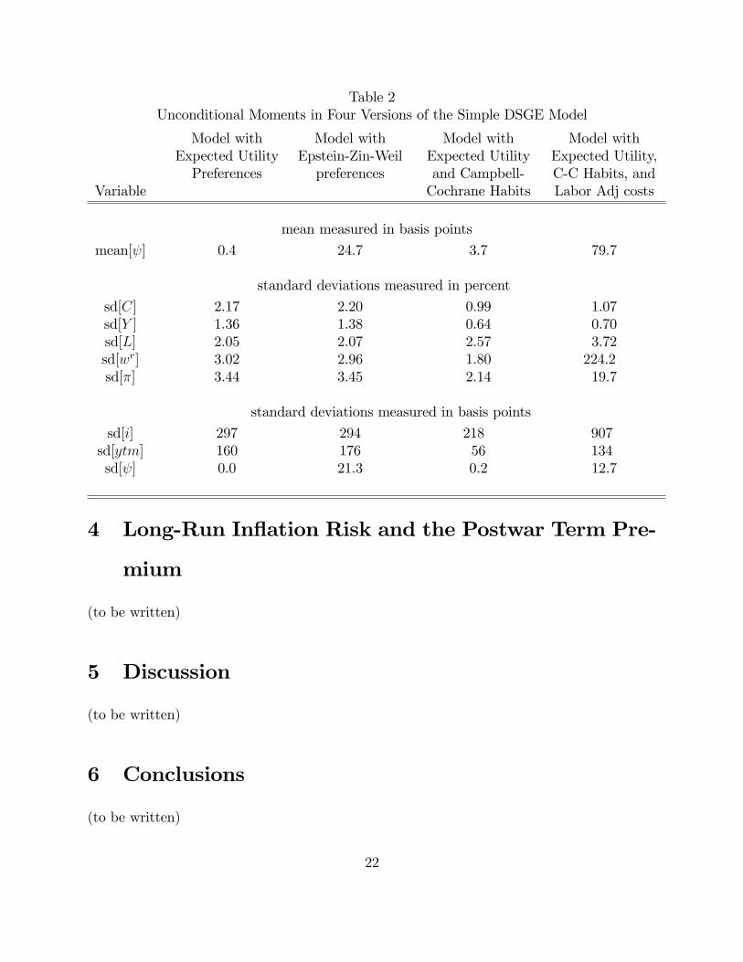
Table 2Unconditional Moments in Four Versions of the Simple DSGE Model

Model with Model with Model with Model withExpected Utility Epstein-Zin-Weil Expected Utility Expected Utility,Preferences preferences and Campbell- C-C Habits, and

Variable Cochrane Habits Labor Adj costs

mean measured in basis points

mean[ ] 0.4 24.7 3.7 79.7

standard deviations measured in percent

sd[C] 2.17 2.20 0.99 1.07sd[Y ] 1.36 1.38 0.64 0.70sd[L] 2.05 2.07 2.57 3.72sd[wr] 3.02 2.96 1.80 224.2sd[�] 3.44 3.45 2.14 19.7

standard deviations measured in basis points

sd[i] 297 294 218 907sd[ytm] 160 176 56 134sd[ ] 0.0 21.3 0.2 12.7

4 Long-Run In�ation Risk and the Postwar Term Pre-

mium

(to be written)

5 Discussion

(to be written)

6 Conclusions

(to be written)

22

References

[1] Altig, David, Lawrence Christiano, Martin Eichenbaum, and Jesper Lindé (2004),�Firm-Speci�c Capital, Nominal Rigidities, and the Business Cycle,� manuscript,Northwestern University.

[2] Backus, David, Allan Gregory, and Stanley Zin (1989), �Risk Premiums in the TermStructure,�Journal of Monetary Economics 24, 371�99.

[3] Backus, David, Bryan Routledge, and Stanley Zin (2007), �Asset Prices in BusinessCycle Analysis,�unpublished manuscript, Columbia Business School.

[4] Bansal, Ravi and Ivan Shaliastovich (2008), �Risk an Return in Bond, Currency, andEquity Markets,�unpublished manuscript, Duke University.

[5] Bansal, Ravi and Amir Yaron (2004), �Risks for the Long Run: A Potential Resolutionof Asset Pricing Puzzles,�Journal of Finance 59, 1481�1509.

[6] Blanchard, Olivier and Jordi Galí (2005), �Real Wage Rigidities and the New KeynesianModel,� NBER Working Paper 11806.

[7] Boldrin, Michele, Lawrence Christiano, and Jonas Fisher (2001), �Habit Persistence,Asset Returns, and the Business Cycle,�American Economic Review 91, 149�66.

[8] Calvo, Guillermo (1983), �Staggered Prices in a Utility-Maximizing Framework,�Jour-nal of Monetary Economics 12, 383�98.

[9] Campbell, John and John Cochrane (1999), �By Force of Habit: A Consumption-BasedExplanation of Aggregate Stock Market Behavior,�Journal of Political Economy 107,205�51.

[10] Campbell, John and Robert Shiller (1991), �Yield Spreads and Interest Rate Move-ments: A Bird�s Eye View,�Review of Economic Studies 58, 495�514.

[11] Christiano, Lawrence, Martin Eichenbaum, and Charles Evans (2005), �Nominal Rigidi-ties and the Dynamic E¤ects of a Shock to Monetary Policy,�Journal of Political Econ-omy 113, 1�45.

[12] Cochrane, John (2001), Asset Pricing (Princeton: Princeton University Press).

[13] Cochrane, John (2007), �Financial Markets and the Real Economy,�in Handbook of theEquity Risk Premium, edited by Rajnish Mehra, Amsterdam: Elsevier, 237�330.

[14] Cochrane, John and Monika Piazzesi (2005), �Bond Risk Premia,�American EconomicReview 95, 138�60.

23

[15] Den Haan, Wouter (1995), �The Term Structure of Interest Rates in Real and MonetaryEconomies,�Journal of Economic Dynamics and Control 19, 909�40.

[16] Donaldson, John, Thore Johnsen, and Rajnish Mehra (1990), �On the Term Structureof Interest Rates,�Journal of Economic Dynamics and Control 14, 571�96.

[17] Epstein, Lawrence and Stanley Zin (1989). �Substitution, Risk Aversion and the Tem-poral Behavior of Consumption and Asset Returns: A Theoretical Framework.�Econo-metrica 57, 937�69.

[18] Erceg, Christopher, Dale Henderson, and Andrew Levin (2000), �Optimal MonetaryPolicy with Staggered Wage and Price Contracts,�Journal of Monetary Economics 46,281�313.

[19] Fama, Eugene and Robert Bliss (1987), �The Information in Long-Maturity ForwardRates,�American Economic Review 77, 680�92.

[20] Gallmeyer, Michael F., Burton Holli�eld, and Stanley E. Zin (2005), �Taylor Rules,McCallum Rules and the Term Structure of Interest Rates,�Journal of Monetary Eco-nomics 52, 921�50.

[21] Gürkaynak, Refet, Brian Sack, and Eric Swanson (2005), �The Sensitivity of Long-Term Interest Rates to Economic News: Evidence and Implications for MacroeconomicModels,�American Economic Review 95, 425�36.

[22] Jermann, Urban (1998), �Asset Pricing in Production Economies,�Journal of MonetaryEconomics 41, 257�75.

[23] Kreps, David and Evan Porteus (1978), �Temporal Resolution of Uncertainty and Dy-namic Choice Theory,�Econometrica 46, 185�200.

[24] Levin, Andrew, Alexei Onatski, John C. Williams, and Noah Williams (2005), �Mon-etary Policy Under Uncertainty in Micro-Founded Macroeconometric Models,�NBERMacro Annual, 229�87.

[25] Lettau, Martin and Harald Uhlig (2000), �Can Habit Formation Be Reconciled withBusiness Cycle Facts?�Review of Economic Dynamics 3, 79�99.

[26] Mehra, Rajnish and Edward Prescott (1985), �The Equity Premium: A Puzzle,�Journalof Monetary Economics 15, 145�61.

[27] Piazzesi, Monika and Martin Schneider (2006), �Equilibrium Yield Curves,� NBERMacro Annual, 389�442.

[28] Rudebusch, Glenn D., Brian Sack, and Eric Swanson (2007), �Macroeconomic Implica-tions of Changes in the Term Premium,�Federal Reserve Bank of St. Louis, Review 89,241�69.

24

[29] Rudebusch, Glenn D. and Eric Swanson (2007), �Examining the Bond Premium Puzzlewith a DSGE Model,�unpublished manuscript, Federal Reserve Bank of San Francisco.

[30] Rudebusch, Glenn D., and Tao Wu (2004), �A Macro-Finance Model of the Term Struc-ture, Monetary Policy, and the Economy,�manuscript, Federal Reserve Bank of SanFrancisco, forthcoming in the Economic Journal.

[31] Smets, Frank, and R. Wouters (2003), �An Estimated Stochastic Dynamic GeneralEquilibrium Model of the Euro Area,� Journal of European Economic Association 1,1123�75.

[32] Swanson, Eric, Gary Anderson, and Andrew Levin (2006), �Higher-Order Perturba-tion Solutions to Dynamic, Discrete-Time Rational Expectations Models,�manuscript,Federal Reserve Bank of San Francisco.

[33] Tallarini, Thomas (2000), �Risk-Sensitive Real Business Cycles,�Journal of MonetaryEconomics 45, 507�32.

[34] Wachter, Jessica (2006), �A Consumption-BasedModel of the Term Structure of InterestRates,�Journal of Financial Economics 79, 365�99.

[35] Weil, Phillipe (1989), �The Equity Premium Puzzle and the Risk-Free Rate Puzzle,�Journal of Monetary Economics 24, 401�21.

[36] Woodford, Michael (2003), Interest and Prices: Foundations of a Theory of MonetaryPolicy, Princeton University Press.

25