Inflation Risk and the Inflation Risk Premium*

Electronic copy available at: http://ssrn.com/abstract=1600312

Inflation Risk and the Inflation Risk Premium*

Geert Bekaert

Columbia Business School

Xiaozheng Wang

Criterion Economics

April 6, 2010

*This article was presented at the Economic Policy Panel meeting in Madrid, April 2010. This article has benefitted from the suggestions from participants at the “Index Leningen” Conference, organized by Netspar and the Dutch Ministry of Finance in February 2009, and especially from Frans de Roon, Roel Beetsma and Serge Vergouwe, and from the detailed comments of two anonymous referees and the Editor, Philip Lane.


Abstract

This article starts by discussing the concept of “inflation hedging” and provides some estimates of “inflation betas” for standard bond and well-diversified equity indices for over 45 countries. We show that such standard securities are poor inflation hedges. Expanding the menu of assets to foreign bonds, real estate and gold only improves matters marginally. This indicates a potentially important role for inflation index linked bonds. We then briefly discuss the pros and cons of such bonds, focusing the discussion mostly on the situation in the US, which started to issue Treasury Inflation Protected Securities (TIPS in short) in 1997. We argue that it is hard to negate the benefits of such securities for all relevant parties, unless the market in which they trade is highly deficient, which was actually the case in its early years in the US. Finally, we describe how state-of-the-art term structure research has tried to uncover estimates of the inflation risk premium. Most studies, including very recent ones that actually use inflation-linked bonds and information in surveys to gauge inflation expectations, find the inflation risk premium to be sizable and to substantially vary through time. This implies that governments should normally lower their financing costs through the issuance of index-linked bonds, at least in an ex-ante sense.


1

INTRODUCTION

In an imperfectly indexed monetary world, inflation risk is one of the most important economic risks, faced by consumers and investors alike. Individuals saving for retirement must make sure their wealth finances their expenses in retirement, whatever the inflation scenario. The liabilities of pension funds and endowments are likely to increase in nominal terms with inflation1. While the world has enjoyed relatively mild inflation during the last decade, the recent crisis has made market observers and economists wonder whether inflation will rear its ugly head again in years to come. Central banks across the world have injected substantial amounts of liquidity in the financial system and public debt has surged everywhere. It is not hard to imagine that inflationary pressures may resurface with a vengeance once the economy rebounds.

It is therefore quite important to ask whether inflation risk can be easily hedged in financial markets. In fact, in a number of countries, governments have issued securities, linked to an inflation index, which makes the hedging more or less perfect. The existence of a sizable government inflation-linked bond market typically spurs the development of inflation derivative contracts, which could satisfy more complex inflation–linked hedging demands. This development in turn has instigated a debate on the benefits and costs, both for investors and for the government, of inflation-linked securities. A critical element in such a debate is the notion of the inflation risk premium, the compensation demanded by investors, for not being perfectly indexed against inflation, or, put differently the insurance premium investors pay governments to shoulder the inflation risk. There is apparently no consensus about the magnitude of this premium, with some recent articles even suggesting it to be negative (see, e.g., Grishchenko and Huang (2008))! The uncertainty surrounding the inflation risk premium also means that there is uncertainty about critical inputs in any strategic asset allocation, such as the real returns on cash and bonds and their correlation with other asset returns.

This paper accomplishes three things. First, it discusses the concept of “inflation hedging” and provides some estimates of “inflation betas” for standard bond and well-diversified equity indices for over 45 countries. We show that such standard securities are poor inflation hedges. When we expand the menu of assets to foreign bonds, real estate and gold, matters only improve marginally. Generally speaking it appears easier to hedge inflation risk in emerging markets than it is in developed markets. This indicates a potentially important role for inflation index linked bonds in developed markets. Second, we briefly discuss the pros and cons of such bonds, focusing the discussion mostly on the situation in the US, which started to issue Treasury Inflation Protected Securities (TIPS in short) in 1997. We argue that it is hard to negate the benefits of such securities for all relevant parties, unless the market in which they trade is highly deficient, which was actually the case in its early years in the US. Finally, we describe how 1 We will ignore the important issue that official estimates of inflation are unlikely to represent an adequate representation of the relevant price changes for a particular investor. For example, endowments should likely focus on the cost inflation for items dominating their budgets, such as professors’ salaries and real estate expenses.

2

state-of-the-art term structure research has tried to uncover estimates of the inflation risk premium. While we focus primarily on the findings in one study (Ang, Bekaert, Wei (2008)), we end the discussion with a survey of recent results that try to bring more data to the table, both in terms of inflation-linked bonds and survey data on inflation expectations. We provide some recent estimates of the inflation premium in the US, the UK and the euro area. The final section concludes.

I. Inflation Hedging

For existing securities to be good inflation hedges, their nominal returns must at the very least be positively correlated with inflation. Nevertheless, there are several ways to define the “inflation hedging capability” of a security. Reilly, Johnson and Smith (1970) examine whether a security protects real purchasing power over time, by calculating the incidence of negative real returns. Clearly, higher yielding assets will almost surely do well on such measure, but may not prove good inflation hedges in the short run, if they fail to generate high returns at times when inflation is high, especially when it is unexpectedly high. Bodie (1976) measures how the variance of the real return of a nominal bond can be reduced using an equity portfolio as a gauge of the hedging capability of equities. In this article, we consider a very simple concept of inflation hedging, namely, the inflation beta, computed using a simple regression:

Nominal return = α + β inflation + ε (1)

Here, ε is the part of the return not explained by inflation. If β = 1, the security is a perfect hedge against inflation. Note that it is conceivable that even a perfectly indexed security does not generate a perfect coefficient of 1 in the regression in (1). This is true because inflation may be correlated with value-relevant factors that are omitted from the regression. We discuss one such important factor, namely a measure of economic activity, in further detail below. Furthermore, an imperfect but stable and predictable relation between a security's return and inflation could suffice for hedging (see Schotman and Schweitzer (2000)), as it would be trivial to compute a hedge ratio. We examine the stability of the relationship explicitly below. Nevertheless, hedging may be difficult to accomplish in practice (especially if it involves short positions), and such hedge portfolios are not likely easily and cheaply accessible to retail investors. It remains therefore interesting to examine how strongly an asset’s return comoves with inflation and whether it reacts one to one inflation shocks, as measured by the inflation beta in (1).

I.1 Inflation Betas of Stocks and Bonds

How do the main asset classes fare in terms of inflation hedging capability? We obtained nominal government bond returns, nominal stock returns and inflation data for over 45 countries. A data appendix contains more details, but the sample period for most series ends in January 2010, whereas the starting point varies from country to country, between January 1970 and January 2005. Generally, the data are more extensive for stocks than for bonds, and for

3

developed markets than for emerging markets. We look at logarithmic annual returns, computed from monthly data. Using monthly data but a one-year horizon, results in the residuals of the regression analysis reflected in Equation (1) exhibiting positive serial correlation. We correct the standard errors for this using the standard approach advocated by Hansen and Hodrick (1980).

Exhibit 1 shows the betas from the regression in (1) for bond returns. Dark bars indicate that the beta is statistically significantly different from 1 (at the 10% level). We find that 19 out of 48 inflation betas are indeed significantly below 1, a further 5 countries exhibit negative betas, which are not statistically significantly different from 1. So in half the countries, bond returns react reliably negatively to inflation, earning negative returns in period of high inflation. This should not be surprising. While expected inflation should be priced into the return on bonds, they will be particularly sensitive to shocks to unexpected inflation. We actually examine this further below. Note that in another 8 countries the betas are below 0.5, meaning that real returns react quite negatively to inflation shocks.

But should stocks not fare better? After all, they are real securities, and whereas there are many ways in which inflation could be value relevant for equities it is difficult to argue in favor of a particular bias. There is already a rather voluminous literature on US data showing that equities are not particularly good inflation hedges; in fact the nominal returns of stocks in the US and inflation are mostly negatively correlated.2 In Exhibit 2, we extend this evidence to 48 countries. The inflation beta in the US is indeed negative but it is not statistically significantly below 1. In fact, the coefficient became less negative by adding the recent crisis years, in which low stock returns and below average inflation went hand-in-hand. In any case, real returns on stocks and inflation are solidly negatively correlated in the US for a sample extending from 1970 to the beginning of 2010. However, the US is not the exception but rather the rule. The majority of the inflation betas are negative, and of the ones that are positive, most are way too low. In 15 countries, we observe inflation betas that are significantly below one, and in a further 16 countries the betas are negative but not significant. In only 12 countries is the inflation beta close to one in statistical and economic terms (say, higher than 0.5) or implausibly high as in Morocco or Hungary.

To get a more survey feel for the results, Exhibit 3 presents the results for “pooled regressions.” Here the inflation beta is estimated using all countries, allowing for a country specific intercept, but allowing only one beta per (regional) group.3 Bonds exhibit inflation betas that are mostly positive but significantly below 1, at least in developed countries, meaning that their real returns are low when inflation is high. The inflation betas are higher in emerging countries, and the

2 One classic paper is Fama (1981). In fact, bond yields and equity yields (dividend or earnings yields) are surprisingly highly correlated in the US, reflecting the strong negative response of equity returns to inflation; see Bekaert and Engstrom (2010) for more discussion and a potentially rational explanation.

3 We actually estimate two regressions, one for the developed/emerging split-up, and then another one for all the other groups.

4

pooled beta is indistinguishable from 1. The result seems to be mostly driven by Latin-America, as the inflation beta for bonds in Asia and Africa are negative. The picture is similar for stocks, in that here too the inflation betas are closer to one for emerging markets than for developed markets. The main difference is that stock returns are negatively correlated with inflation for all developed markets, a result largely driven by North America and Oceania. In the EU, the correlation is small, but not significantly different from 1. The positive coefficient for emerging markets is again driven by the Latin-American countries, as the correlation between inflation and stock returns is negative in both Asia and Africa.

The overwhelmingly positive coefficients on nominal bonds may give the impression that bonds are “not so bad,” but of course they likely reflect the effect of previously expected inflation being priced into bonds and inflation being persistent over time. The right hand side of Exhibit 3 reports results from a multi-variate regression, regressing the returns onto two variables, expected inflation the year before and unexpected inflation (the difference between realized and expected). In Fama and Schwert (1977), a classic paper on inflation hedging, they call an asset a complete hedge against inflation if it has coefficients equal to one on both variables in this regression.

Of course this regression requires an estimate of expected inflation! It is impossible to come up with accurate measures of expected inflation for all the countries in this sample, so we use a very simple procedure: we let expected inflation at time t be current year-on-year inflation at t. While this random walk model for inflation may appear inconsistent with the data, we suspect it is hard to beat by more complex models in out-of-sample forecasting. In fact, for the US, Atkeson and Ohanian (2001) show as much.4 The table simply reports the coefficient on the second component, unexpected inflation (which is really just the change in inflation). With only a few exceptions, we obtain what was to be expected: the unexpected inflation betas are further removed from 1 than were the “total” inflation betas. This suggests that whatever link with inflation does exist comes through its expected part. For stock returns, all the betas are now negative except for Latin-America (where the beta is still indistinguishable from one), but the Latin-American region still drives the coefficient to 1 for emerging markets as a whole.

All of our results apply to one-year returns; this is a reasonable horizon to investigate, even when considering long-horizon investors, as portfolios are typically rebalanced at least once a year. However, it is conceivable that the inflation hedging capability of stock returns is more apparent at longer horizons, and, in fact, Boudoukh and Richardson (1993) claim that stocks constitute a better hedge for inflation at longer horizons. In Exhibits 4 and 5, we examine this issue for our extensive set of countries. We only consider pooled results for the larger groups here, as the

4 The US inflation time series seems to exhibit ARMA(1,1) type behavior at the monthly frequency. However, there is evidence of parameter instability in the coefficients, and there is strong seasonality in monthly data. Both features of the data complicate an application to a set of international data where many samples are quite short. As we discuss later, for the US, Ang, Bekaert and Wei (2007) demonstrate that professional surveys provide the best forecasts. Such surveys are obviously not available for most countries in our sample.

5

longer horizons start exhausting the degrees of freedoms for many countries. Exhibit 4 contains the inflation betas. For bond returns, the coefficients are nicely increasing with horizon and they are insignificantly different from 1 at the 5 year horizon for developed markets, and well over 1 for emerging markets. Perhaps this is not entirely surprising, as it may simply reflect the accuracy of longer term inflation expectations. The result may also reflect a strong cross-country dimension (bond yields in high inflation countries being reliably higher than bond yields in low inflation countries). For stock returns, the developed market betas increase with horizon but remain significantly below 1, even at the 5 year horizon. For emerging markets, they show little horizon dependence and are just about 1. The unexpected inflation betas, shown in Exhibit 5, tell a different story, however. While the betas for bonds still increase with horizon, they remain significantly below 1 for developed markets, even at the 5-year horizon. For stocks, the betas remain significantly negative for all groups, except for emerging markets.

The negative relation between stock returns and inflation is the topic of a literature too vast to fully survey here. Suffice it to say that many recent articles rely on money illusion to explain this empirical relationship (see, e.g. Campbell and Vuolteenaho, 2004). However, the literature has also identified a number of rational channels, all of which have important consequences for the interpretation of the regression ran before. Fama (1981)’s proxy hypothesis essentially argues that the stock market anticipates economic activity and if inflationary periods coincide with periods of low economic activity, a negative relationship between stock and bond returns results. Bekaert and Engstrom (2010) find some evidence in favor of the proxy hypothesis, but suggest that the bulk of the correlation between stock returns and inflation occurs through a discount rate channel. In recessions, risk premiums increase and hence, stagflationary periods may induce a negative inflation – stock return relationship. Liu’s (2009) finding that inflation uncertainty has a negative effect on stocks in 16 developed countries is also suggestive of a discount rate channel. Finally, Doepke and Schneider (2009) focus on the redistributive effects of inflation. Episodes of unanticipated inflation reduce the real value of nominal claims and thus redistribute wealth from lenders to borrowers. Because borrowers are younger on average than lenders, an unanticipated inflation shocks generates a decrease in labor supply as well as an increase in savings, hence reducing output. All these channels suggest that the relationship between inflation and stocks returns may largely reflect a relationship between the stock market and a measure of economic activity. The stagflation stories of Fama (1981) and Bekaert and Engstrom (2010) suggest that how much the relationship between economic activity and stock markets affects the inflation-stock return comovement depends on the incidence of stagflations in a particular country.

To examine this effect in more detail, we obtained data on industrial production growth for most of our countries. We could not find adequate data for 8 countries in our sample. Therefore, Exhibit 6 displays both the original inflation beta from a univariate regression (which only differs from the estimate in Exhibit 3 because the country set may be slightly different), and the beta on inflation in a bivariate regression, including industrial production growth as an additional independent variable. The results are stark. For both bond and stock returns, the inflation betas

6

invariably increase, often becoming substantially larger than 1. For quite a few country groups, the coefficients are now not statistically different from 1. Given that economic activity correlates positively with the stock market, this implies that on average the negative correlation between inflation and the stock market reflects a negative correlation between economic activity and inflation. This strongly suggests that the relationship between economic activity, inflation and the stock market deserves further attention. It also explains why the recent crisis episode, with low inflation during bad economic times, has in fact increased the comovement of inflation and stock returns.

I.2 Inflation Betas for Other Asset Classes

Many other assets have been suggested as potentially good inflation hedges. In this section, we expand the menu of assets to foreign bonds, real estate, and gold. The return variation of foreign bonds is dominated by variation in currency values. Because long-term changes in currency values tend to reflect long-term relative inflation rates—that is, Purchasing Power Parity is a reasonable long-term model for exchange rates- foreign bonds may provide good insurance against inflation shocks, at least in the medium to long run. To avoid proliferation of potential assets to investigate, we create an equally-weighted index of 4 major bond markets, representing the 4 major currency blocks: the dollar, the euro (deutsche mark), the pound and the yen. That is, we create an index of US, German, UK and Japanese government bonds. For the US, Germany, the UK and Japan, only three foreign bonds are used in the portfolio.

For many households, a house represents the ultimate “real” asset. However, the use of residential house prices would entail a host of data and interpretative problems that we want to avoid here. Therefore, we obtained data from EPRA, the European Real Estate Organization, which maintains an extensive international data set on publicly traded real estate companies. Nevertheless, our data sample is reduced to 25 instead of 46 countries, and the earliest starting point for the return series is January 1990.

Finally, commodities have recently started to become a popular alternative asset class and may potentially serve as a natural hedge for inflation. If commodity prices are an important driver of inflation movements, it is conceivable that commodity price index changes may be highly correlated with general inflation. However, it is not that obvious that commodities really constitute a great inflation hedge. First, the relationship between commodity prices and actual inflation is complex, and varies through time. For example, in the past, oil price shocks typically passed through powerfully into general inflation, but more recently their effect has been more subdued, perhaps because of increased globalization, or competitive effects through “cheap” Chinese exports abroad. Whatever it may be, the relationship does not appear stable over time. More importantly, exposure to commodities is typically accomplished through commodity futures. However, it is not clear at all that the returns to commodity futures, which are essentially contracts in zero net supply, are highly correlated with inflation. Erb and Harvey (2006) show that while an index of commodity futures returns had a positive and significant unexpected inflation beta, its different components have betas that vary wildly across different

7

commodities, and are often counterintuitive. They suspect that the inflation beta is not stable at all over time. They also note that even a broad-based commodity futures index excludes many items measured in actual consumer price indices, used to compute inflation. Consequently, commodity futures are not likely effective inflation hedges. Nevertheless, gold has recently again received much popular attention as the safe asset that should protect against inflation shocks. We therefore obtained data on both spot gold prices (the GSCI index), and data on returns earned by going long gold in the futures market. For the latter, we actually use a total return index including the return on cash using T-bills.5 We simply compute gold price changes to approximate the return on holding gold physically. Note that all gold returns and gold prices are in dollars and must be converted into local currency to assess their inflation hedging capability for each country. Hence, gold’s hedging ability may also be due to currency movements, rather than to changes in gold prices per se.

The inflation betas for these three asset classes are contained in Exhibits 7 through 9. Exhibit 7 considers inflation and unexpected inflation betas at the one year horizon, pooled over various country groups. For foreign bonds, the coefficients are now invariably positive and mostly not significantly different from 1. Hence, foreign bonds provide decent hedges for inflation shocks. This remains true for unexpected inflation shocks with the exception of North America, where the slope coefficient is -0.06, albeit very imprecisely estimated. The evidence for real estate is decidedly more mixed. The inflation beta is positive for North America, but negative for all other country groups for which we have data. For unexpected inflation betas, the coefficient also becomes positive for Asia. The inflation betas of gold investments are invariably positive and often quite large, especially for unexpected inflation betas. Of course, except for North-America, these comovements may also partially reflect the hedging properties of foreign exchange exposure. Exhibits 8 and 9 show the inflation and unexpected inflation betas, respectively, also for 3- and 5-year horizons. For foreign bonds, the betas either show little horizon variation (emerging markets), or they increase with the horizon. For example, the negative unexpected inflation beta for North America turns positive at the 5 year horizon, and becomes insignificantly different from 1. The real estate betas also increase with horizon. For gold the picture is more mixed, but in any case all betas are substantially positive at all horizons. A striking feature of all these results is that for emerging markets, inflation betas appear quite close to one, at all horizons. One possible interpretation is that inflation risk is relatively speaking a much more important risk in these economies that drives much of the variation in asset returns, whereas in developed markets, the relationship is much more fragile.

A contemporaneous article by Attié and Roache (2009), mostly focusing on the US but containing some international results, mostly confirms our findings. Bonds, equities and real estate have negative unexpected inflation betas, but gold and commodities have positive betas. Using a vector autoregressive framework, they find that it is difficult to protect a portfolio against unexpected inflation in the long term as well using traditional asset classes.

5 We thank Campbell Harvey for providing the gold price and futures data.

8

I.3 The Stability of Inflation Betas

The large cross-sectional variation of inflation betas across country groups and horizons, given our varying sample sizes, may also reflect parameter instability. There are many reasons for the betas to change through time. We already discussed that an omitted variable such as economic activity may make the inflation beta hard to interpret and depend on the incidence of stagflations during the sample. An obvious and related cause for instability is the monetary policy regime. Recently, a great many countries have adopted explicit or implicit policies of inflation targeting, which may have caused inflation expectations to be more anchored and lower (see Mishkin and Schmidt-Hebbel (2001)), and more generally have changed its stochastic properties, including its correlation with asset returns. We would also expect that a pro-active monetary policy would affect the hedging efficiency of index-linked bonds as it would lower inflation volatility and increase real interest rate volatility, potentially leading to higher correlations between nominal and index-linked bonds. To examine this possibility informally, we consider a very simple exercise. For the full country sample, we consider a break date in 1990, estimating different betas for the two periods. This implies that the latter part is likely dominated by inflation targeting regimes and more active monetary policies.

Exhibit 10 contains the results. Note that the Emerging, Latin-America and Africa results are missing, because our data typically start after 1990. We do have an emerging category for stocks, but the number of data points before 1990 is relatively limited. Panel A reports the inflation betas for three different horizons. For bonds, the betas generally decrease, even turning negative from positive in a few cases (Asia and North America). One exception is non-EU Europe where the betas increase. The decrease in beta is significant at the 1% level for the developed markets group, for Asia and for the EU countries. For stocks we observe the same decreasing beta phenomenon, except for the EU countries. Here, the decrease in beta is significant for the emerging markets group, for Latin America, Asia and for Oceania. The longer horizon betas follow qualitatively a similar pattern. Panel B reports the unexpected inflation betas. There, we see the opposite phenomenon for bonds, with betas typically increasing post 1990. They mostly remain negative though, and the change is never significant at the 5% level. Looking over different horizons, the pre-1990 betas increase strongly with horizon, but the post 1990 betas mostly increase only slowly with horizon. Consequently, at long horizons, several unexpected inflation betas are significantly below 1, and they decreased significantly relative to pre-1990 betas in several cases. For stock returns, there are no clear patterns in the betas across time, and for the longer horizon betas, only one test rejects stability at the 5% level (the Asia group). For the one year horizon however, there is a significant change in beta at the 5% level for 5 country groupings, the steep decreases in beta for North America and the EU being the most striking.

For the US, we can collect data going even further back than 1970. We collected bond and stock returns from 1960 onwards. Exhibit 11 reports break tests for the US, using 4 different break dates: the beginning of 1973, the start of a turbulent stagflationary period with two oil shocks;

9

1980, the date often mentioned by monetary economists as representing a break in monetary policy from accommodating to more active (see Boivin (2006) and Moreno (2004)); and finally 1990 and 2000. The results are perhaps surprising: there are almost no significant breaks in the coefficients. Where we do see some significance (at the 5% and 10% levels) is for the unexpected inflation beta of bonds and stocks with 1980 as the break point. We see that the bond beta becomes more negative and the stock beta less negative. If the negative stock return inflation relationship reflects stagflationary periods, we would indeed expect it to be less prevalent after 1980. Moreover, the break in 2000, with the coefficient going from almost -4.0 to 2, is no surprise either, given the recent crisis. The bond result is somewhat hard to interpret, the more that the beta post 1990 and 2000 is again substantially less negative. In other words, the negative coefficient is really driven by the 1980s, and could perhaps be associated with the Volcker period, after which agents were positively surprised by inflation decreasing faster than expected.

In future work, it would be interesting to link the stability test more directly to monetary policy regimes, e.g. by specifying the break dates as dates at which inflation targeting was adopted. In addition, a country specific measure of beta stability (e.g. the variance of a rolling beta estimate) could be linked cross-sectionally to country characteristics, such as the nature of a country’s monetary policy, its economic and financial development, the variability of inflation, etc. We defer this to future research.

I.4 Tracking Inflation

While one security by itself may not prove a particularly good inflation hedge, it is possible that a portfolio of several securities hedges inflation quite well. To investigate this possibility, we create an inflation mimicking portfolio from our menu of our assets, a government bond index, a foreign bond index, the local stock market, gold returns, gold futures return, and a real estate index. Because gold spot and futures returns are substantially correlated, the gold futures series is eliminated from the portfolio. To find the inflation mimicking portfolio, we minimize the variance of the residuals of a regression of inflation on the asset returns, where the regression coefficients are constrained to add to one. This can be interpreted as a minimum variance portfolio problem, and we solve for the asset weights using simple covariance formulas. We explicitly do not constrain the weights to be positive, as the fact that the portfolio problem wants to short an asset is particularly informative. An Appendix provides more technical background.

We conduct this exercise for each country; and Exhibit 12, Panel A averages the portfolio weights over various country groups. The weights reveal that real estate is rarely useful in hedging inflation. The other assets all obtain somewhat meaningful positive weights for certain sub-groups. There are distinct differences between developed and emerging markets. For developed countries, the inflation mimicking portfolio consists primarily out of domestic bonds and gold, but for emerging markets, domestic and foreign bonds make up the bulk of the portfolio.

10

Of course, a rather simple asset that may track inflation well is a Treasury bill. Nominal short rates should reflect expected inflation and rolling over short-term Treasury bills may suffice to protect against inflation. We obtained monthly data on Treasury bill rates for most of our countries. While the maturity of the T-bills is mostly three months, we assume that the term structure is flat at the short end, and roll over a monthly rate over the course of a year to compute the annual return on a Treasury bill. In Panel B, we see that when such Treasury bills are added to the menu of assets, they receive most of the portfolio weight. Only for non-EU Europe do other assets play a meaningful role.

While it is tempting to conclude that Treasury bills are the ideal asset to track inflation, it is important to realize that the portfolio problem minimizes a variance. The problem with the inflation mimicking exercise is that most asset returns are more variable than inflation, so that the positive weights may also reflect to a large extent the variance reducing properties of the assets, rather than their ability to hedge inflation risk. This may explain why domestic bonds are relatively ‘attractive” in the first exercise, and it certainly explains why Treasury bills receive weights close to 1 in Panel B, as they simply are by far the lowest variability asset. To see this more clearly, in Panel C, we simply report the results from an unconstrained mimicking problem (which is equivalent to regressing inflation on the various asset returns and recording the coefficients). We also report the R2, the variability of the “portfolio return” divided by the variance of inflation. These R2’s tend to be larger for emerging markets than for developed markets, but this, unfortunately, does not necessarily reflect the existence of a better hedge portfolio. Most of the asset weights are actually negative! For emerging markets, foreign bonds receive positive weights here and there; for developed markets, T-bills have small positive weights. For domestic bonds, the highest coefficient observed is barely 1%; for stocks all coefficients for all country groups are negative! In short, it is next to impossible to use an individual asset or a portfolio of assets to adequately hedge inflation risk.

A recent article by Bruno and Chincarini (2010) attempts a similar portfolio tracking exercise for a slightly different menu of assets, while also requiring a certain minimum real return. They also find a role for Treasury bills and no role at all for equities, but their results may also be driven by the variance reducing properties of Treasury bills.

II. TIPS to the rescue

Index-linked bonds protect investors against the risk of inflation by indexing the cash flows of the bonds to an inflation index. Consequently, such bonds potentially provide an important role in helping investors hedge an important economic risk. Here we provide a short summary of the potential benefits and costs of inflation protected bonds, ending the section with a brief survey of the experiences in the US, the UK and the Euro area. Lengthier discussions of the pros and cons of indexed debt with references to some of the quite old theoretical literature on the topic can be

11

found in Campbell and Shiller (1996), Price (1997), Garcia and van Rixtel (2007) and Roush, Dudley and Ezer (2008).

II.1 General Benefits of Inflation Protected Bonds

Market completeness, diversification and risk sharing. Because other securities are so imperfectly correlated with (unexpected) inflation, such bonds truly help financial markets become more complete, in the sense that financial markets should provide the possibility of getting payoffs under as many economic contingencies as possible. Given differences in risk aversion across investors, the co-existence of indexed bonds and of non-indexed bonds with inflation risk (and presumably higher returns), allows for overall better risk sharing (see Campbell and Shiller (1996) for an elaborate discussion). This would make them almost surely overall welfare enhancing. It is also likely that the government is better able to shoulder inflation risk than individual investors (see van Ewijk (2009)), and it is even conceivable that indexed bonds would encourage people to save more, thereby potentially affecting the overall savings rate, and therefore economic growth.

Even if other securities could be used to (partially) hedge inflation risk, the existence of a long-term real safe asset, would appear of great benefit to individual and institutional investors, especially if they have long-term liabilities. Institutional investors, such as pension funds and endowments, typically formulate a long-term (“strategic”) asset allocation policy over broad asset classes. TIPS would constitute a perfect separate class: they represent a homogenous set of securities, likely displaying relatively low correlation with other assets, as there does not exist any other security that indexes away inflation risk. Moreover, at least in theory, we would expect the addition of TIPS to raise the “utility” of the investor. For the aforementioned institutional investors, who typically use mean variance optimization to determine strategic asset allocations, TIPS should increase the optimal Sharpe ratio.

Market information on inflation expectations and real rates. As we discuss in more detail later, TIPS may potentially help provide market-based information on important economic variables, such as real interest rates and inflation expectations over different maturities. Such information is helpful for investors and policy makers alike. Moreover, because this information is gleaned from market prices, it is available in real time, without any lag (as opposed to, for example, survey data on expected inflation).

Debt Savings. If investors indeed fear inflation risk and demand compensation for incurring it when investing in nominal government bonds, the “inflation risk premium” will be positive and an inflation index-linked bond will cost less to issue than a nominal bond of similar maturity, thereby reducing the debt costs of the government. As Campbell and Shiller (1996) point out, from a society’s perspective, it is not at all clear that the government should try to minimize its financing costs. Nevertheless, it is quite likely that index-linked bonds may help to generate smooth, predictable financing costs in real terms, thereby averting distortionary taxation, which would be welfare enhancing (see also Roush, Dudley and Ezer, 2008).

12

Inflation Credibility. The existence of inflation-indexed bonds may even reduce the government’s incentives to inflate (see Campbell and Shiller (1996)), although Fischer (1981) marshals some evidence that indexed bonds increase an economy’s sensitivity to price shocks. For the developed markets that have recently introduced TIPS, this would appear less important to begin with, as the central banks that set monetary policy should be independent of the Treasury (see Garcia and Van Rixtel, 2007).

II.2 Costs to Issuing Inflation Protected Bonds

There is no doubt that TIPS markets have become increasingly important in many industrialized countries over the last decade, often experiencing rapid growth. Bloomberg now lists over 40 countries with index-linked debt, and major countries such as the UK, the US, France, Australia, Canada and Japan all have important TIPS programs. The existence of a government benchmark bond curve has spurred a thriving market in privately provided inflation derivatives in the US and Europe. Yet, in all these markets, with the exception of the UK, the inflation-linked market still accounts for a minor if rising part of government debt. Given the distinct economic benefits of TIPS, why is that the case? Are governments reluctant to supply the bonds private agents are clamoring for, or are they simply sensing that the private demand does not warrant creating a new security? After all, the index-linked programs started in a period of relatively low global inflation and inflation expectations.

It is likely impossible to even answer this question, but a critical examination of whether the theoretical benefits always hold in practice can provide a useful perspective.

Market completeness, diversification and risk sharing. If other financial assets were good inflation hedges, the case for indexed securities would be less compelling. We believe that our empirical evidence strongly suggests this is not the case, but opinions may differ and investors may mistakenly believe that their house, or gold investments will adequately protect them against inflation shocks. Briere and Signori (2009), for example, claim that inflation-linked bonds in the US no longer provide meaningful diversification benefits relative to nominal bonds post 2003. From the government’s perspective, there are, of course, real costs involved in setting up a new program to issue bonds, indexed to inflation. Therefore, the benefits must be substantial enough to motivate expending the costs. Ensuring that the market is viable takes time, effort and commitment and it may not work. For example, in Japan, local institutional investors have proved very reluctant to invest in index-linked bonds (see Kitamura, 2009). If the welfare benefits are dramatic, you may wonder why not more private entities have issued index-linked bonds, and why the private market cannot create an inflation derivatives market by itself. Yet, the existence of a default – free benchmark is likely too important for this to happen. Finally, it is conceivable that certain governments feel they already shoulder too much inflation risk through other programs, such as Social Security programs.

Market information on inflation expectations and real rates. Most major central banks appear to make use of the information provided by TIPS markets; yet the interpretation of TIPS yields is

13

far from simple. While they should represent a market reading on real interest rates, if the market has relatively poor liquidity, the TIPS rate may also reflect a liquidity premium, which may vary through time. We come back to this issue extensively in the next section. Moreover, gleaning information about inflation expectations by comparing nominal and real rates is not only complicated by this liquidity premium, but also by the potential presence of an inflation risk premium.

Debt Savings. A reduction in debt costs is far from guaranteed. First, the inflation risk premium theoretically need not be positive (see, especially, Campbell, Shiller and Viceira (2009)). Second, the new securities may lack liquidity, leading investors to demand a liquidity premium which drives up issuance costs. We return to both issues in the next section.

Inflation Credibility. The original argument against inflation-indexed bonds, especially in inflation prone countries, is that they would lead to less commitment to fight inflation, as indexed bonds made its effects less onerous. This argument seems of no consequence for the industrialized countries that introduced TIPS recently, which all have independent central banks, keen on establishing anti-inflation credibility.

II.3. Concrete Experiences with TIPS

Here we offer some quick comments on the experiences of three developed markets with inflation –protected bonds, the UK, France and the Euro area, and finally, the US, on which we focus most attention. This is warranted as the US TIPS market has become the largest index-linked market with over $500 billon outstanding at the end of 2008.

The UK. The UK program is the oldest program, with the UK government issuing indexed Gilts since 1981. Importantly, the index-linked market is an important part of the total gilt market, representing close to 30% of the total market at the end of 2008, making it the largest index-linked program in relative terms. Changes in UK financial regulation did prove critical in further boosting demand for indexed gilts. The Pension Act of 2004 requires pension funds to prove that they can meet their future liabilities, which has led to a strong demand for long-dated indexed gilts.

Deacon and Andrews (1996) estimate that, from the year of their introduction in 1982, to 1993, indexed Gilts ex-post reduced the cost of issuing government debt, and that, ex-ante, the cost should be lower as the inflation risk premium is likely positive. Nevertheless, they also mentioned the presence of a positive liquidity premium making index-linked bonds more expensive than nominal bonds. Reichsretter (2008) still claims that nominal bonds embedded an ex-ante risk premium for the 1984-2006 period, but indexed bonds did not, indicating there is indeed a positive inflation risk premium, which may lead to government savings in issuing indexed debt.

The Euro area and France. France first introduced indexed Treasury bonds (the so-called OATis) in 1998. An issue of special interest in the Euro area is to what inflation index these

14

bonds should be indexed. France first used its local CPI, excluding tobacco. Later on, it started to issue bonds indexed to the HPIC (the Harmonized Index of Consumer Prices), again excluding tobacco. The HPIC is the euro-wide price index in terms of which the quantitative definition of price stability is defined and it is regularly published by Eurostat. This index has now become the market benchmark in the euro area, with other countries issuing inflation –linked bonds indexed to that index (Italy, Greece and Germany) and financial products (swaps, futures) linked to it as well. The euro-area government linked bond market has now overtaken the UK market to become the second largest linker market in the world behind the US, both in terms of outstanding amounts and turnover (see Garcia and van Rixtel (2007) for some relevant data). As we will discuss in more detail in the next section, while the index linked market in the Euro area may continue to experience rapid growth, initially there were teething problems, and the market was not very liquid. Yet, Bardong and Lehnert (2004) claim that even in its early days the market provided efficiency benefits in a mean-variance context.

A very important issue within the Euro area is whether there should be bonds indexed to country specific CPI indices, or whether any country issuing inflation-linked debt should use the euro-wide HPIC. We believe that there are good reasons to use the euro wide index. First, the experiences of various index-linked programmes teach us that it is not easy to build a liquid, well-accepted bond market. Standardization should enhance liquidity, deepen the market, and further spur the development of derivative contracts. Second, there is empirical evidence that inflation rates have substantially converged within the EU (see, e.g., Bekaert and Wang, 2009), although, there is no guarantee that future events will not lead to occasional divergences.

The US. The US started issuing TIPS in 1997. While the TIPS program in the US initially met with some enthusiasm (see Sack and Elsasser (2004)), the program grew rather slowly. Exhibit 13 shows the outstanding amount of TIPS, which grew from around $150 billion at the end of the nineties to close to $500 billion at the end of 2008. The Treasury affirmed its commitment to the program in 2002.

TIPS only gained very slow traction with individual investors. The left-hand side scale of Exhibit 13 shows the growth in assets under management in mutual funds focusing on TIPS, which was very gradual till about 2004, then accelerated to reach over 80 billion at the end of 2008. TIPS were more of a success among institutional investors. In fact, many pension funds and endowments in the US decided to create a new strategic asset class, comprising TIPS. For example, one of the largest endowments, Harvard Management Company (HMC henceforth) introduced TIPS as a new asset class with a 7% strategic asset allocation in 2000.6

As we argued before, it made perfect sense to introduce TIPS as a new asset class. The team at HMC concluded that TIPS increase the optimal Sharpe ratio, and formal research by Kothari and

6 See Viceira (2000) for an excellent Harvard case on the introduction of TIPS at HMC, which provided the source of some of the HMC material here.

15

Shanken (2004) and Roll (2004) also suggest that TIPS would receive an important weight in an efficient portfolio.

But, not all was well with TIPS. An asset class should also have a sufficiently large market capitalization to absorb the demands of institutional and other investors and its market environment should show sufficient liquidity to allow active trading. Both conditions were not likely satisfied in the early years of the TIPS market. We come back to this important issue below. These problems potentially undermine some of the purported benefits of TIPS. For example, extracting information about real yields proved difficult. As a concrete example, when Harvard Management Company, in 2000, introduced TIPS as a new asset class, it changed its long-run real interest rate from 2% to 3.5%. The primary reason was that its analysts observed real yields in the TIPS market substantially higher than 2%, and more of the order of 4%. This decision reflected two important errors in setting capital market assumptions. First, it is not a great idea to estimate a long-run return using only a few years of data. Not only is there much sampling error, but, as we further discuss below, many returns show cyclical patterns, which call for a sample period that “goes through a few cycles.” In addition, even in ideal circumstances, real yields will reflect market participants expectations of future inflation which may not be borne out in actual data and inflation forecasting errors cannot be expected to average to zero over such a short period. Second, the TIPS market back then was in its infancy, not very liquid and perhaps even a somewhat “unknown, inefficiently priced” asset, as suggested by Sack and Elsasser (2004). We argue below that in the beginning of the TIPS issuance period, likely up to 2004, real interest rates were much lower than suggested by TIPS data,7 because of a liquidity premium.

This rather substantial liquidity premium, which we return to in detail in the next section, implies that ex-post the US Treasury likely increased its debt costs relative to issuing nominal bonds (see Roush, Dudley and Ezer (2008); and Campbell, Shiller and Viceira (2009)).

The HMC saga also re-iterates the need for set of stylized facts regarding real interest rates, expected inflation and their relation. Of key interest is the inflation risk premium. In the following section, we decompose nominal yields into three economically important components. We then discuss how the recent term structure literature has attempted to identify these components and summarize some concrete estimates.

7 Of course, it is questionable that historical data should be used at all in setting capital market assumptions for expected returns. It may be better to “reverse engineer” them from an equilibrium model such as the CAPM (see Sharpe (1976)). In that case, TIPS should be part of the optimal portfolio proportional to their relative market capitalization.

16

III. The Inflation Risk Premium

III.1Definition and General Identification

The inflation risk premium is the compensation investors demand to protect themselves against inflation risk. To understand how the inflation risk premium relates to bond yields, consider the following equation:

n nt t t t n, n t, ny r E [ ] (2)

n et t, nr

Here, n

ty is the yield on a nominal zero-coupon bond of maturity n; ntr is the yield on a perfectly

indexed zero coupon bond of maturity n. The difference between the two is often called “inflation compensation” or sometimes “breakeven inflation rate,” as it constitutes the inflation rate that ex-post would make the nominal yields on both bonds equivalent. Inflation compensation economically consists out of two components. The first is simply expected inflation; the second is the inflation risk premium.

A well-known theory of interest rate determination due to Fisher (1930), holds that the inflation risk premium ought to be zero. If true, there is no expected benefit to the government of issuing inflation protected securities. While actual inflation may differ from expected at any given time, unless systematic biases exist, the inflation surprises should cancel out over time, so that there is no expected benefit or cost to issuing TIPS over Treasuries. Most believe there is indeed an inflation risk premium. However, it need not be positive. While it is tempting to conclude that the inflation risk premium is linked to the uncertainty or volatility of inflation, its economic determinants are, in most modern pricing models, in fact a bit more subtle. It is easy to show that the inflation risk premium should be positive if inflation is high in “bad times.” If inflation would always occur when agents are exceedingly happy, they would not need an inflation risk premium.8 Of course, this correlation between the wealth or consumption of agents and inflation may well vary through time, and cause substantial correlation in the conditional inflation risk premium. Campbell, Shiller and Viceira (2009) note that the current positive

8 In the parlance of modern finance, what is required is a positive correlation between the real “pricing kernel” and inflation. The pricing kernel takes on high values in bad states of the world, because risk averse economic agents want to move consumption and wealth into these states, and they are therefore relatively expensive. In alternative models, pure uncertainty about future states of the world may generate risk premiums as well.

inflation risk premium

expected inflation

inflation compensation

real rate

nominal rate

break-even inflation rate

17

correlation between inflation and stock returns (as an indicator of “wealth”) may well mean that the inflation premium is now negative in the US.

How can we identify the different components? At first blush, it looks like an easy task. Indexed

bonds would deliver ntr ; inflation forecasts could deliver the second term, and subtracting both

of the obviously observable nominal yields gives us an estimate of the inflation risk premiums, for any horizon we fancy. Unfortunately, it is not that easy. TIPS have only existed for about 13 years, and, as we argue below, the first 7 years are likely not usable in any estimation. Inflation forecasting is at best an imprecise and difficult business. So, we are left with data on nominal yields and actual (not expected) inflation in most cases, although more recent studies have tried to expand the information used (see below). In other words, en econometrician would not view the task as easy but as impossible!

Over the years, a great many approaches have been used to identify the components in Equation (2). It is fair to say that in modern asset pricing, techniques have converged to the following approach:

i. Formulate a no arbitrage term structure model that prices nominal and real bonds. The no arbitrage condition ensures that the pricing is consistent across the curve and across time. The modeling involves a stochastic process for a “pricing kernel” that prices the bond‘s payoffs and is consistent with a number of economic principles and stochastic processes for a number of “factors,” that are deemed relevant for pricing the term structure (TS, henceforth). In some standard models, these factors could be the “level”, “slope”, and “curvature” of the yield curve.

ii. Formulate an inflation model and link it to the TS model. This model should be consistent with data on inflation and hopefully, in conjunction with term structure data, yield accurate expected inflation numbers.

iii. Estimate the model using as much data as possible, but data on inflation and nominal bond yields are a must.

The estimated model will then imply an inflation risk premium, which immediately reveals a potential problem. The model has to be general enough so as to not impose restrictions on the findings, but it will nonetheless have to be restricted so as to achieve identification of essentially three unobserved components with two sets of information (nominal yields and inflation). We come back to this identification problem below, and a Box provides some additional intuition.

III.2. Stylized facts regarding real rates and inflation risk premiums in the US

A recent example of the just-described approach is Ang, Bekaert, Wei (2008). They use a no-arbitrage term structure model, that prices real and nominal bonds and make the model quite general. First, the model explicitly allows for the possibility that risk premiums may vary

18

through time, for example, with the business cycle. Second, the model accommodates “regime switches” in interest rates. Many TS studies have shown that the behavior of interest rates can abruptly change, causing regimes in volatilities and persistence. Such changes can be generated by monetary policy changes or reflect business cycle variation, for example. Finally, the model allows arbitrary correlation between real rates and (expected) inflation. They use quarterly inflation and term structure data to estimate the model over a fairly long period, 1952:Q1 – 2004:Q4. This is important, as short samples may give a much distorted view of long-term inflation risk premiums, especially if these premiums vary through time.

The approach of Ang, Bekaert and Wei (2008) (ABW, henceforth) is to consider a large number of different models (24 in total), and to select the model that best fits the data (term structure data, inflation data and their correlation). From this exercise, they can then extract a set of stylized facts regarding real interest rates, expected inflation and the inflation risk premium.

While not the focus of our discussion here, let us mention that ABW find that the term structure of real rates is, unconditionally, hump shaped: it is fairly flat around 1.24%, with a slight hump, peaking at a 1-year maturity. Real rates are quite variable at short maturities, consistent with an activist monetary policy buffeting short rates to affect inflation expectations, but smooth and persistent at long maturities. Campbell, Shiller and Viceira (2009) argue that TIPS in the US provide desirable insurance against future variation in real rates and therefore may carry a negative real term premium. In the UK, recent evidence of declining real term premiums has been linked to demand pressures from institutional investors needing very long-duration real exposure to hedge liabilities,9 and perhaps similar factors may play a role in the US as well. Nevertheless, formal estimates for the UK with data from 1983 to 1999 (see Risa, 2001) uncover solidly positive real term premiums.

Since the real rate curve is rather flat10 and the nominal yield curve in the US is on average upward sloping, there must be, on average, a positive inflation risk premium that is increasing in maturity. Note that this is only true “on average,” because then expected inflation cannot have a maturity component, but at any given point of time, inflation expectations can also increase with maturity. Exhibit 14 shows some properties of the inflation risk premium. The fact that the premium is about zero at the one quarter maturity is not a finding of the article, but rather an imposed assumption to help overcome the identification problems imposed by Equation (2). It is clear that the inflation risk premium is generally positive and increases to over 1% at the 5 year horizon. ABW found two “inflation regimes,” a “normal” regime where inflation is relatively high and the inflation risk premium substantial, and a regime in which inflation is decreasing (a disinflation regime) and inflation risk premiums are much smaller.

9 More specifically, a government rule, implemented in 2005, requires UK pension funds to mark their liabilities to market, using discount rates derived from government bonds (see Campbell, Shiller and Viceira (2009), pp.8-9).

10Roll (2004) studies actual data on TIPS and finds the real curve to be flatter than the nominal curve.

19

Exhibit 15 graphs the 5-year inflation risk premium over time. In general, the premium rose very gradually from about 75 basis points until the late 70s, before entering a very volatile period during the monetary targeting period from 1979 to the early 1980s. It is then that the premium reached a peak of 2.04%. From then onwards, the trend appears downward, but with some rather big swings. During the late 1990s equity bull market, the inflation premium remained relatively stable around 1%, then dropped to a low of 0.15% after the 2001 recession. Fears of deflation were apparent then. At the time of writing, the severe recession has significantly depressed the inflation risk premium. The long history in Exhibit 15 shows that the inflation risk premium has often decreased in recessions but it also shows that this situation may not last! It is surely conceivable that part of the variability we observe is due to estimation error (note the relatively wide confidence bands around the estimates!), but alternative estimates for the US (Buraschi and Jiltsov (2007), for example), and for the UK (Risa (2001)) document similar variability in the inflation risk premium.

Because pension funds often have a long-term view, it is of interest to compute inflation risk premiums for bonds with a longer duration. In the ABW model, zero coupon bonds of maturity 10 (20) years carry an inflation risk premium of 112 (84) basis points on average. 11

The ABW paper has a number of other interesting findings. For example, the decompositions of nominal yields into real yields and expected inflation at various horizons indicate that variation in expected inflation and inflation risks premiums explains about 80% of the variation in nominal rates at both short and long maturities. That is, the folklore wisdom that “inflation is more important in the long run” is not quite true. Inflation is really an important level factor in the term structure that affects both the short and long end of the curve. However, when one focuses on spreads (and essentially eliminate this level factor), the importance of inflation compensation for spreads does increase with maturity and becomes very dominant at the long end of the maturity spectrum.

BOX: Identification in No Arbitrage Term Structure Models.

In most no-arbitrage term structure models, there are a number of exogenous factors or state variables driving the term structure, which are typically assumed to follow a particular stochastic process (say, a Gaussian vector autoregression), with a particular heteroskedasticity structure. In addition, there is a stochastic process for the “pricing kernel,” which prices all bonds. A strictly positive pricing kernel imposes no arbitrage, so that the pricing kernel is always modeled in logs. In an economic model, the pricing kernel would correspond to the Intertemporal Marginal Rate

11 We thank Min Wei for computing these numbers. She also provided longer-duration numbers for the D’Amico, Kim and Wei (2008) article, discussed in the next section.

20

of Substitution. The pricing kernel will contain the shocks to different factors multiplied by coefficients (these may be even time-varying processes) that capture how the shocks are “priced,” the so-called “prices of risk.” Because the model contains latent variables, a first identification problem is simply to ensure that these variables are uniquely identified, requiring a number of parametric restrictions on the processes (see Dai and Singleton (2000) for a discussion of how to accomplish this for affine models). For example, it is well known that you need at least N+1 bonds to identify N prices of risk. If you want to identify one price of risk, both a short bond and a long bond are necessary and the term spread helps identify the price of risk. Non-linearities, such as present in the ABW–model, may actually help identification.

The models discussed in the text differ from standard models, as the real and nominal side is differentiated. The nominal pricing kernel must be (in logs) the real pricing kernel minus inflation, and an observable series, inflation, is added to the mix of data. The inflation time series by itself, and the assumption of rational expectations, can often suffice to identify expected inflation. Without data on TIPS however, nominal term spreads and their correlation with inflation must somehow identify both the inflation risk premium and real rates. Given a sufficient number of bonds, and a sufficiently parsimonious model, this is theoretically feasible, but often practically infeasible. It is often the case that the effect of key prices of risk parameters on real rates and on the inflation risk premium is similar and of opposite magnitude, making the average level of both indeterminate. To circumvent this problem, ABW imposed the inflation risk premium to be zero at the quarterly horizon. They then estimated a great many possible models and selected the best performing model to provide a decomposition of nominal yields into their three components. With another assumption on the one period inflation risk premium, the average level of real rates and the average level of the inflation risk premium would change accordingly. Models that can bring information from TIPS and/or inflation forecasts to bear on the estimation problem obviously greatly reduce such identification problems.

------End Box------

III.3. Recent estimates of the inflation risk premium

The disadvantage of the ABW study is that it only uses nominal bond data and data on inflation. It would be obviously useful to test their findings with estimates that are informed by more data, in particular by data on inflation linked bonds. Recent research has tried to resolve the identification problem in Equation (2) by using data in index-linked bonds, and additional, exogenous information on inflation forecasts present in survey data.

The Use of TIPS. Let me first address the use of index-linked bonds. With the exception of the UK, index-linked bonds in most developed countries have a fairly short history. This by itself limits their usefulness in extracting long-term inflation expectations and risk premiums. It is important, given the tremendous time-variation in inflation risk premiums discussed above, to

21

use a fairly long history in assessing properties of the inflation risk premium. In the US, we now have data on TIPS since 1997, which really does not represent sufficient data by itself, but the actual situation is worse, because of the poor liquidity of the TIPS market in its infancy years. Exhibit 16 shows the secondary market trading in TIPS over time. It increased tenfold, almost twice as much as the amount of TIPS outstanding. Bid-ask spreads in the TIPS market have decreased over time as well; market participation and turnover have generally increased. There is general agreement that the liquidity in the TIPS market has improved dramatically (see Roush, Dudley and Ezer (2008) for a detailed discussion). Moreover, the commitment made by the US government to the TIPS program in 2002 helped resolve market uncertainty about the asset class. Today, the TIPS market is liquid, but still not as liquid as the Treasury bond market. This creates a tremendous problem for the use of TIPS data in uncovering real yields. Denote zero

coupon rates derived from TIPS, as n,TIPStr . They can be thought of as consisting out of two

components:

n,TIPS n nt t tr r LiQPR (3)

where LiQPR represents a liquidity premium that may vary through time. The literature contains a number of liquidity premium estimates. Exhibit 17 presents a graph of the estimate by D’Amico, Kim and Wei (2008). They compare a term structure model with and without TIPS to infer liquidity premiums. The liquidity premium is very large in the first 4 to 5 years (well over 1%), and then declines to hover below 50 basis points now. Gurkaynak, Sack and Wright (2007) provide an alternative estimate, which shows the same secular decline, with again 2004 the critical year where liquidity premiums become relatively small. 12

Nevertheless, the difference in liquidity between Treasuries and TIPS remains an issue even to date. When there is a flight to safety, as there is in the current crisis, investors flock to the most liquid security and liquidity premiums rise. This means that the most recent TIPS data may again reflect a sizable liquidity premium. This liquidity problem is not limited to the US, but exists for the Euro area and even for the UK as well, bid-ask spreads are invariably larger for the index-linked bonds, and time-varying liquidity premiums exist.

The Use of Survey Forecasts. In many countries, there exist surveys of inflation forecasts by professionals and consumers. In the US, there are a number of well-known surveys, with data going back quite a while, including the Livingston survey, the Michigan survey (consumers), and the SPF survey (Survey of Professional Forecasters). Without a lengthy historical record, it is hard to test the accuracy of the forecasts. In a recent article, Ang, Bekaert and Wei (2007) examine in much detail the quality of various forecasting methods for one year ahead annual inflation. In particular, they examine the out-of-sample forecasting performance of four different types of forecasting methods: time series models (which use past data on inflation to forecast

12 The Federal Reserve Bank of Cleveland developed its own procedure to compute the liquidity risk premium but acknowledged it was no longer of practical use during the current crisis.

22

future inflation); Phillips curve models (which link expected inflation to some measure of the “output gap”, a business cycle indicator); term structure models (which use nominal interest rates to forecast future inflation) and surveys, as mentioned above.

While one of the most successful models here is the random walk model, which simply uses the current inflation rate to forecast future inflation, ABW’s main result is quite simple: Surveys consistently beat other models in terms of “root mean squared error;” that is, the square root of the average squared forecasting errors. There are many potential reasons for the superior forecasting performance of the surveys: they may aggregate more information from more sources than is possible in most models, or may reflect information not present in any model (e.g. regarding policy decisions); they can also respond quickly to new information, whereas most models must assume some stability of existing relationships. ABW conjecture that the surveys perform well for all of these reasons: the pooling of large amounts of information, the efficient aggregation of this information and the ability to adapt quickly to major changes in the economic environment such as the drop in real volatility of the mid-eighties known as the Great Moderation, and now perhaps, the crisis conditions. This research suggests that the decomposition in (2) would benefit from using information in the surveys.

Recent Estimates of the Inflation Risk Premium. With this in mind, we searched the literature for recent studies that provide estimates of the inflation risk premium, using either information in inflation-linked bonds or surveys, or both. Exhibit 18 mentions the studies and the various estimates for different maturities. Studies that use TIPS data before 2004 necessarily underestimate the inflation risk premium. That is because the high real interest rates really reflected liquidity premiums, but not true real interest rates. The one US study that reports an average inflation risk premium that is negative (Christensen, Lopez, and Rudebusch (2008)) suffers from this problem. In fact, they report negative inflation premiums before 2004 and positive ones thereafter. The picture emerging from the other 4 studies mentioned, however, is that the inflation risk premium is robustly positive. The magnitude differs, varying between 50 and over 200 basis points at the 10 year horizon. The larger estimates are more in line with previous studies, such as Buraschi and Jiltsov (2005), and Campbell and Viceira (2001).13

We also mention a few European studies. Both Hordahl and Tristani (2007) and Garcia and Werner (2008) find a very modest inflation premium of only 25 basis points at the 5 year horizon. However, it is likely that this low estimate reflects the short sample period which was characterized by relatively subdued inflation. My personal estimate of a long-term inflation risk premium for the euro area would be substantially larger. For the UK, where a long history of index-linked debt is available, we mention a recent study by Joyce, Lundholdt and Sorensen (2008), which does not report an average inflation risk premium, but does graph it over time. The graph confirms much of what was claimed in this study: the inflation risk premium is mostly

13 The estimate in Buraschi and Jiltsov (2005) is on average 70 basis points; in Campbell and Viceira (2001), albeit using a slightly different but related definition based on holding period returns, the estimate is 110 basis points.

23

positive, can be large, and varies considerably over time. Older studies, such as Evans (1998, 2003), stress the importance of time-varying inflation risk premiums in the UK, but surprisingly do not report estimates of their magnitude. There is one other, unpublished study by Risa (2001), which fits an affine term structure model to UK nominal and index-linked gilts for data spanning 1983 to 1999. His inflation risk premium estimates exceed does reported for the US by ABW (2008)!

IV. Conclusions

This article has made a number of relatively simple points about inflation risk. First, standard securities, such as nominal government bonds and equities are very poor hedges of inflation risk, both in the short and in the long run. We estimated inflation betas for a very large cross-section of countries, showing that this is nearly universally true. When we expand the work to include real estate, foreign bonds and gold, the latter two fare a little better, often showing positive comovement with inflation. Nevertheless, tracking inflation with available securities seems to be quite difficult to do. As a consequence, index-linked bonds are essential to really hedge inflation risk.

With index linked bonds, investors, policymakers and economists can have a better sense of the magnitude of the inflation risk premium, the compensation investors demand to bear inflation risk in nominal bonds. Most studies, including very recent ones that actually use inflation-linked bonds and information in surveys to gauge inflation expectations, find the inflation risk premium to be sizable and to substantially vary through time.

This implies that governments should normally lower their financing costs through the issuance of index-linked bonds, at least in an ex-ante sense. However, some index-linked markets, and in particular the US market, have suffered from poor liquidity driving up real yields, and increasing the cost of issuance. While several measures can be taken to improve liquidity in the index-linked market, recent events demonstrate once again that in volatile market conditions, investors gravitate towards the most liquid securities (typically nominal Treasury bills and benchmark bonds) and liquidity premiums can become extremely large. Wright (2009) and Campbell, Shiller and Viceira (2009) discuss in detail the anomalous behavior of the TIPS markets following the Lehman Brothers collapse of September 2008, with yields on TIPS rising above yields on their nominal counterparts at one point. From the government’s perspective such episodes undermine some of the purported benefits of index-linked debt. For central banks, the information content of the spread between real and nominal bonds becomes more difficult to interpret in economic terms; and the benefits in terms of debt costs are no longer ensured. The policy implication is that much effort must be expended to ensure that the TIPS market is credible, liquid, and trusted by important investors, but even then, occasional but hopefully short-lived flights to liquidity may occur.

24

From an economic perspective, such considerations seem less relevant. Having securities that allow the hedging of an important economic risk are almost surely welfare enhancing, and the investors in such securities (individuals, pension funds) tend to have long horizons, and are thus surely not unhappy with the presence of a potential liquidity premium. Without the government setting a default free benchmark, it is unlikely that “inflation-derivatives”, which have grown rapidly, recently, would spring up in private markets. Therefore, the case for an index-linked market would appear easy to make.

25

References

Ang, A., G. Bekaert, and M. Wei (2008), “The term structure of real rates and inflation expectations,” Journal of Finance, Vol. 63 (2), 797-849

Ang, A., G. Bekaert, and M. Wei (2007), “Do Macro Variables, Asset Markets or Surveys Forecast Inflation Better?” Journal of Monetary Economics, 54, 1163-1212

Atkeson, A. and L. Ohanian (2001), “Are Phillips Curves Useful for Forecasting Inflation?”, Federal Reserve Bank of Minneapolis Quarterly Review, Winter, 25:1.

Attié, A.P. and S.K. Roache (2009), “Inflation Hedging for Long-Term Investors,” IMF Working Paper.

Bardong, F. and T. Lehnert (2004), “On the Efficiency of European Inflation-Indexed Government Debt Security Markets,” Journal of Portfolio Management, 30(4), 226-238.

Barro, R. (1974), “Are Government Bonds Net Wealth?” Journal of Political Economy, 82:6, 1095-1117.

Bekaert, G. and Engstrom, E. (2010), “Inflation and the Stock market: Understanding the ‘Fed Model’ ”, Journal of Monetary Economics, forthcoming.

Bekaert, G. and X. Wang (2009), “Globalization and Asset Prices,” Working Paper.

Bodie, Z. (1976), “Common Stocks as a Hedge Against Inflation,” Journal of Finance, 31, 459-470.

Boivin, J. (2006), “Has US Monetary Policy Changed? Evidence from Drifting Coefficients and Real-Time Data,” Journal of Money, Credit and Banking, 38:5, 1149-1173.

Boudoukh, J. and M. Richardson (1993), “Stock Returns and Inflation: A Long-Horizon Perspective,” The American Economic Review.

Briere, M. and O. Signori (2009), “Do Inflation-Linked Bonds Still Diversify?” European Financial Management 15:2, March, 279-297.

Buraschi, A. and A. Jiltsov, (2005), “Inflation Risk Premia and the Expectations Hypothesis,” Journal of Financial Economics, 75, 429-90.

Campbell, J.Y. and R. Shiller (1996), “A Scorecard for Indexed Government Debt,” in Ben S. Bernanke and Julio Rotemberg eds. National Bureau of Economic Research Macroeconomics Annual 1996, MIT Press: Cambridge, MA, 155–197.

26

Campbell, J.Y., R.J. Shiller, and L. Viceira (2009), “Understanding Inflation-Indexed Bond Markets,” Working Paper.

Campbell, J.Y. and L. Viceira (2001), “Who Should Buy Long-Term Bonds?” American Economic Review, 91, 99-127.

Campbell, J.Y. and T. Vuolteenaho (2004), “Inflation Illusion and Stock Prices,” American Economic Review, 94, 19-23.

Chen, R. –R., B. Liu and X. Cheng (2005), “Inflation, Fisher Equation, and the Term Structure of Inflation Risk Premia: Theory and Evidence from TIPS,” Working Paper, Rutgers Business School.

Chernov, M. and P. Mueller (2007), “The Term Structure of Inflation Forecasts,” Working Paper.

D’Amico, S., Kim, D. and Wei, M. (2008), “Tips from tips: The Information content of Treasury inflation-protected security prices,” Finance and Economics Discussion Series Working Paper 2008-30, Federal Reserve Board.

Dai, Q. and K. Singleton (2000), “Specification Analysis of Affine Term Structure Models,” Journal of Finance 55:5, 1943-1978.

Deacon, M. and P. Andrews (1996), “The Use and Value of Index-Linked Bonds,” The Financier 3:4-5, 13-25.

Devarajan, S., V. Swaroop and H. Zou (1996), The Composition of Public Expenditure and Economic Growth, Journal of Monetary Economics, 37:2, 313-44.

Doepke, M. and M. Schneider (2006), “Inflation as a Redistribution Shock: Effects on Aggregates and Welfare,” Working Paper.

Erb, C. and C. Harvey (2006), “The Strategic and Tactical Value of Commodity Futures,” Financial Analysts Journal, 62:2, 69-97.

Evans, M.D.D. (1998), “Real Rates, Expected Inflation, and Inflation Risk Premia,” Journal of Finance, 53: 187-218.

Evans, M.D.D. (2003), “Real Risk, Inflation Risk, and the Term Structure,” Economic Journal, 113: 345-389.

Fama, E.F. (1981), “Stock Returns, Real Activity , Inflation, and Money,” American Economic Review, 74:4, 545-565.

Fama,.E.F. and G.W. Schwert (1977), “Asset Returns and Inflation,” Journal of Financial Economics 5, 115-146.

27

Fisher, I. (1930), The Theory of Interest. Reprinted 1965, Clifton, NJ: Augustus M. Kelley.

Garcia, J.A. and A. van Rixtel (2007), “Inflation-Linked Bonds from a Central Bank Perspective,” ECB Working Paper.

Garcia, J.A. and T. Werner (2008), “Inflation Risks and Inflation Risk Premia,” ECB Working Paper.

Grishchenko, O. and J. Huang (2008) “Inflation Risk Premium: Evidence from the TIPS Market,” Working Paper

Gurkaynak, R., B. Sack, and J. Wright (2007), “The Tips Yield Curve and Inflation Compensation,” Working Paper.

Hansen, L.P. and R.J. Hodrick (1980), “Forward Exchange Rates as Optimal predictors of Future Spot Rates: An Econometric Analysis,” Journal of Political Economy, 88:5, 829-853.

Haubrich, J. G. Pennacchi, and P. Ritchken (2008), “Estimating Real and Nominal Term Structures using Treasury Yields, Inflation, Forecasts, and Inflation Swap Rates,” Working Paper.

Hordahl, P., and O. Tristani (2007), “Inflation risk premia in the term structure of interest rates,” BIS Working Paper.

Joyce, M., P. Lildholdt, and S. Sorensen (2007), “Extracting Inflation Expectations and Inflation Risk Premia From the Term Structure: A Joint Model of the UK Nominal and Real Yield Curves,” Working Paper, Bank of England.

Kothari, S. and J. Shanken (2004), “Asset Allocation with Inflation-Protected Bonds,” Financial Analysts Journal 60, 54-70.

Lin, Shu-Chin (2009), “Inflation and Real Stock Returns Revisited,” Economic Inquiry 47:4, 783-795.

Mehrota, A. and J.R. Sanchez-Fung (2009), “Assessing McCallum and Taylor Rules in a Cross-Section of Emerging Market Economies,” BOFIT Discussion Paper.

Mishkin, F.S. and K. Schmidt-Hebbel (2001), “One Decade of Inflation Targeting in the World: What Do We Know and What Do We Need to Know?” in Norman Loayza and Raimundo Soto, eds., Inflation Targeting: Design, Performance, Challenges (Central Bank of Chile: Santiago): 117-219.

Moreno, A. (2004), “Reaching Inflation Stability,” Journal of Money, Credit and Banking, 36:4, 801-825.

28

Piazzesi, M. and M. Schneider (2008), “Inflation Illusion, Credit, and Asset Pricing,” in J.Y. Campbell (ed.), Asset Pricing and Monetary Policy. Chicago, IL: Chicago University Press, 147-181.

Price, R. (1997), “The Rationale and Design of Inflation-Indexed Bonds,” IMF Working Paper.

Reilly, F.K., G.L. Johnson and R.E. Smith (1970), “Inflation, Inflation Hedges, and Common Stocks,” Financial Analysts Journal, 28:104-110.

Risa, S. (2001), Nominal and Inflation Indexed Yields: Separating Expected Inflation and Inflation Risk Premia, Working Paper.

Roll, R. (2004), “Empirical TIPS,” Financial Analysts Journal, 60:1, 31-53.

Roush, J., W. Dudley and M. Ezer (2008), “The Case for TIPS: An Examination of the Costs and Benefits,” Federal Reserve Bank of New York, Working Paper.

Sack, B. and R. Elsasser (2004), “Treasury Inflation-Indexed Debt: A review of the US Experience,” Economic Policy Review, Vol. 10 (1), 47-63, Federal Reserve Bank of New York.

Schotman, P and M. Schweitzer (2000), Horizon sensitivity of the inflation hedge of stocks, Journal of Empirical Finance 7: 301-315.

Sharpe, W. (1976), “Imputing Expected Returns from Portfolio Composition,” Journal of Financial and Quantitative Analysis, 9:3, 463-472.

van Ewijk, C. (2009), “Index Linked Bonds, Pensions and Government Debt Management,” presentation at Netspar Conference, Den Haag.

Viceira, L. (2000), “The Harvard Management Company and Inflation-Protected Bonds,” Harvard Business School Case 201-053.

Wright, J.H. (2009), Discussion of “Understanding Inflation-Indexed Bond Markets,” mimeo.

29

Data Appendix

Our data are at the monthly level. The inflation data represent CPI data IMF’s International Financial Statistics; the stock return data are from MSCI and the bond return data from Datastream. The government bond indices of all the countries except India reflect all the maturities of the government bonds of that country. The average maturity differs across countries but for major markets it is likely around 7 years. For India, the index only reflects bonds with maturities between 1 and 10 years.

The industrial production data were downloaded from Datastream. When the overall index is not available for a certain country, we collect the manufacturing industry production index.

The real estate data were purchased from EPRA, the European Public Real Estate Association. The FTSE EPRA/NAREIT Real Estate Index Series only include real estate securities (defined as engaged in “the ownership, trading and development of income-producing real assets”) that are traded on an official stock exchange. The table below lists the availability, per country of the various series. All these series are converted to local currency.

For gold, we use the “Bloomberg Generic Gold Price Index” as the spot price. We use the “S&P GSCI Gold Total Return Index” as future prices; this series uses T-bills as collateral. For each country, the gold spot and futures returns are converted from dollars into local currency.

The short interest data represent Treasury bill rates from Datastream and International Financial Statistics, mostly with a 3-month maturity.

The foreign bond returns are derived from local government bond returns and currency values. For each country, we create the local currency return on an equally weighted index of US, German, UK and Japanese government bonds. For the US, Germany, the UK and Japan, only three foreign bonds are used in the portfolio. Finally, for the US, some results for stock and bond returns use a longer sample, starting in January 1960.

Government bond Stock return Real estate return Industrial production14

start end start end Start end start end Industry

Argentina Feb‐96 Dec‐09 Jan‐88 Jan‐10 n/a n/a n/a n/a n/a

Australia Mar‐87 Jan‐10 Jan‐70 Jan‐10 Jan‐90 Nov‐09 Jul‐74 Sep‐07 All

Austria Jan‐85 Jan‐10 Jan‐70 Jan‐10 Apr‐01 Nov‐09 Jan‐70 Jun‐09* All

Belgium Jan‐85 Jan‐10 Jan‐70 Jan‐10 Jan‐90 Nov‐09 Jan‐70 Jun‐09* All

Brazil Jan‐05 Dec‐09 Feb‐90 Jan‐10 n/a n/a Jan‐91 Jul‐09* All

Canada Jan‐85 Jan‐10 Jan‐70 Jan‐10 Jan‐90 Nov‐09 Jan‐70 Jun‐09* All

Chile Jan‐05 Dec‐09 Jan‐88 Jan‐10 n/a n/a Jan‐70 May‐08 Manufacture

China Nov‐04 Jan‐10 Jan‐93 Jan‐10 n/a n/a Dec‐91 Jul‐09 All

Colombia Jan‐05 Dec‐09 Jan‐93 Jan‐10 n/a n/a Jan‐80 Sep‐05 Manufacture

14 Asterisks here indicate that we used de-seasonalized data.

30

Czech Aug‐98 Jan‐10 Jan‐95 Jan‐10 n/a n/a Jan‐93 Jul‐09* All

Denmark Jan‐85 Jan‐10 Jan‐70 Jan‐10 Jan‐92 Nov‐08 Jan‐74 Jul‐09* All

Egypt Jan‐05 Dec‐09 Jan‐95 Jan‐10 n/a n/a n/a n/a n/a

Finland Jan‐89 Jan‐10 Jan‐88 Jan‐10 Jan‐93 Nov‐09 Jan‐70 Jul‐09* All

France Jan‐85 Jan‐10 Jan‐70 Jan‐10 Jan‐90 Nov‐09 Jan‐70 Jun‐09* All

Germany Jan‐80 Jan‐10 Jan‐70 Jan‐10 Jan‐90 Nov‐09 Jan‐70 Jul‐09* All

Greece Apr‐99 Jan‐10 Jan‐88 Jan‐10 Apr‐04 Nov‐09 Jan‐95 Jun‐09* All

Hong Kong Jan‐05 Jan‐10 Jan‐70 Jan‐10 Jan‐90 Nov‐09 n/a n/a n/a

Hungary Feb‐99 Jan‐10 Jan‐95 Jan‐10 n/a n/a Jan‐85 Jul‐09* All

India Jan‐05 Jan‐10 Jan‐93 Jan‐10 n/a n/a Jan‐70 Apr‐09 All

Indonesia Jan‐05 Dec‐09 Jan‐88 Jan‐10 n/a n/a Jan‐01 Jan‐08 Manufacture

Ireland Jan‐85 Jan‐10 Jan‐88 Jan‐10 Jan‐90 Aug‐09 Jan‐76 Apr‐09* All

Israel Jan‐05 Dec‐09 Jan‐93 Jan‐10 n/a n/a Jan‐70 Jun‐09* All

Italy Jan‐89 Jan‐10 Jan‐70 Jan‐10 Jan‐90 Nov‐09 Jan‐70 Jun‐09* All

Japan Jan‐82 Jan‐10 Jan‐70 Jan‐10 Jan‐90 Nov‐09 Jan‐70 Jul‐09* All

Jordan n/a n/a Jan‐88 Jan‐10 n/a n/a Nov‐71 Jul‐09 All

Korea Jan‐05 Jan‐10 Jan‐88 Jan‐10 n/a n/a Jan‐70 Jul‐09* All

Malaysia Jan‐94 Jan‐10 Jan‐88 Jan‐10 n/a n/a Jan‐71 Jun‐09 All

Mexico Jan‐02 Jan‐10 Jan‐88 Jan‐10 n/a n/a Jan‐80 Jun‐09* All

Morocco Jan‐05 Dec‐09 Jan‐95 Jan‐10 n/a n/a n/a n/a n/a

Netherlands Jan‐80 Jan‐10 Jan‐70 Jan‐10 Jan‐90 Nov‐09 Jan‐70 Jun‐09* All

New Zealand Jan‐89 Jan‐10 Jan‐88 Jan‐10 Jan‐05 Nov‐09 Jan‐87 Dec‐07 All

Norway Jan‐89 Jan‐10 Jan‐70 Jan‐10 Jan‐90 Nov‐09 Jan‐70 Jun‐09* All

Pakistan Jan‐05 Dec‐09 Jan‐93 Jan‐10 n/a n/a Jul‐77 Jun‐09 Manufacture

Peru Jan‐05 Dec‐09 Jan‐93 Jan‐10 n/a n/a Jan‐79 Jul‐08 Manufacture

Philippines Jan‐05 Dec‐08 Jan‐88 Jan‐10 n/a n/a Jan‐81 Dec‐08 Manufacture

Poland Jan‐01 Jan‐10 Jan‐93 Jan‐10 Jan‐06 Nov‐08 Jan‐85 Jul‐09* All

Portugal Jan‐93 Jan‐10 Jan‐88 Jan‐10 Jan‐90 Aug‐09 Jan‐70 Jul‐09 All

Russia Mar‐97 Jan‐10 Jan‐95 Jan‐10 n/a n/a n/a n/a n/a

Singapore Jan‐00 Dec‐09 Jan‐70 Jan‐10 Jan‐90 Nov‐09 Jan‐97 Jul‐09 Manufacture

South Africa Sep‐00 Jan‐10 Jan‐93 Jan‐10 n/a n/a Jan‐70 Jul‐09* Manufacture

Spain Jan‐99 Jan‐10 Jan‐70 Jan‐10 Jan‐90 Feb‐09 Jan‐70 Jul‐09* All

Sweden Jan‐85 Jan‐10 Jan‐70 Jan‐10 Jan‐90 Nov‐09 Jan‐70 Jul‐09* All

Switzerland Dec‐80 Jan‐10 Jan‐70 Jan‐10 Jan‐90 Nov‐09 Jan‐95 Dec‐07* All

Taiwan Jul‐00 Jan‐10 Jan‐88 Jan‐10 n/a n/a n/a n/a n/a

Thailand Feb‐05 Jan‐10 Jan‐88 Jan‐10 n/a n/a n/a n/a n/a

Turkey Feb‐03 Jan‐10 Jan‐88 Jan‐10 n/a n/a Jan‐85 Jul‐09* All

U.K. Jan‐80 Jan‐10 Jan‐70 Jan‐10 Jan‐90 Nov‐09 Jan‐70 Jun‐09* All

US Jan‐80 Jan‐10 Jan‐70 Jan‐10 Jan‐90 Nov‐09 Jan‐70 Aug‐09* All

Venezuela Jan‐05 Dec‐09 Feb‐90 Jan‐10 n/a n/a n/a n/a n/a

31

Technical Appendix

For each country i, we compute the following variables:

Monthly logarithmic returns (including dividends and coupons for bonds, stocks and real estate) in month t: ri,t

Returns aggregated over a horizon of h-months: ri,t+h,h = ri,t+h + ri,t+h-1 +… + ri,t+1.

Ignoring dividends and coupons, this return represents the logarithm of the price at t + h minus the logarithm of the price at time t.

Year-on-year inflation in month t: πi,t = ln(CPIi,t / CPIi,t-12), where CPI is the consumer price index.

Inflation over a “k-year” horizon: πi,t+k×12,k×12 = πi,t+k×12 + πi,t+(k-1)×12 +… + πi,t+1×12

Expected inflation for a horizon of k years: πei,t+k×12,k×12 = k πi,t

Unexpected inflation for a horizon of 6 years : πui,t+k×12,k×12 = πi,t+k×12,k×12 – k πi,t

Using these variables, we run both univariate and bivariate regressions. The univariate country-by-country regressions take the following form:

ri,t+k×12,k×12 = αi + βi πi,t+k×12,k×12 + εi,t+k×12,k×12 (A1)

Because we use monthly data, the “overlap” in observations causes the errors to be serially correlated. We therefore adjust the standard errors using the Hansen-Hodrick (1980) method with lag k×12-1.

For the univariate pooled regressions, we run 2 regressions.

ri,t+k×12,k×12 = αi + jj i,t k 12,k 12

j

+ εi,t+k×12,k×12 (A2)

where:

{βj, j=1,2,…,J} = {βdeveloped, βemerging, J=2}, or {βNorth America, βLatin America, βAsia, βAfrica, βOceania, βEU, βNon-EU Europe, J=7}

πji,t+k×12,k×12 = πi,t+k×12,k×12 if country i in group j; 0 otherwise.

Standard errors are again adjusted using the Hansen-Hodrick (1980) method, as generalized to panel data by Devarajan, Swaroop and Zou (1996).

Analogous standard errors are used for the bivariate regressions. The country-by-country regression is:

32

ri,t+k×12,k×12 = αi + γi πei,t+k×12,k×12 + βi πui,t+k×12,k×12 + εi,t+k×12,k×12 (A3)

The bivariate pooled regression can be represented as:

ri,t+k×12,k×12 = αi +j

j i,t k 12,k 12j

( e + βj πuji,t+k×12,k×12) + εi,t+k×12,k×12 (A4)

where

{γj, βj, j=1,2,…,J} = {γdeveloped, γemerging, βdeveloped, βemerging, J=2}, or {γNorth America, γLatin America, γAsia, γAfrica, γOceania, γEU, γNon-EU Europe, βNorth America, βLatin America, βAsia, βAfrica, βOceania, βEU, βNon-EU Europe, J=7}

πeji,t+k×12,k×12 = πei,t+k×12,k×12 if country i is in group j; 0 otherwise.

πuji,t+k×12,k×12 = πui,t+k×12,k×12 if country i is in group j; 0 otherwise.

To describe our estimations more concretely, it is best to distinguish between the country-by-country regressions and the pooled regressions.

For the country-by-country regressions, let yt,h = ri,t+k×12,k×12; xt = [1 πi,t+k×12,k×12] (univariate regression), or xt = [1 πei,t+k×12,k×12 πui,t+k×12,k×12] (bivariate regression); εi,t+k×12,k×12 =ut,h , where we omit the country dimension. Then the regressions become

yt,h = xt β + ut,h where h = k×12 – 1 (A5)

We estimate the regressions by ordinary least squares (OLS). It can be shown that )ˆ( OLST

converges in distribution to N(0,θ), with:

1

1

1

1

11

T

ttt

T

ttt xx

Txx

T ;

1

1

)(ˆ)(ˆh

hjxu jRjR ;

T

jthjthtu uu

TjR

1,, ˆˆ

1)(ˆ ;

T

jtjttx xx

TjR

1

1)(ˆ where T is the sample size for each country i.

For the pooled regressions, let yit,h = ri,t+k×12,k×12; x

it = [0 … 0 1 0 … 0 π1

i,t+k×12,k×12 π2

i,t+k×12,k×12 … πJ

i,t+k×12,k×12] or xit = [0 … 0 1 0 … 0 πe1

i,t+k×12,k×12 πe2i,t+k×12,k×12 … πeJ

i,t+k×12,k×12 πu1i,t+k×12,k×12

πu2i,t+k×12,k×12 … πuJ

i,t+k×12,k×12] where the 1 is in the ith position; εi,t+k×12,k×12 =uit,h. Then the

regressions become

yit,h = xi

t β + uit,h where h = k×12 – 1 (A6)

The vector representation is YNT = XNT β + UNT and it can be shown that )ˆ( OLSNT

converges in distribution to N(0,θ), with:

33

11ˆˆ

NTNTNTNTNTNTNTNT XXXXXX ; NT̂ is symmetric, its lower triangular part

can be written as:

,0

),(ˆ),0(ˆ

, nR

R

a u

u

tnt

otherwise

jTthn

NTtn

1,1,...,2,1

,...,2,1,0

where njN ,...,2,1,1,...,2,1

N

i

T

jt

ihjt

ihtu uu

NTjR

1 1,, ˆˆ

1)(ˆ .

Note that in principle the country samples are unbalanced, and we use as much data as possible. We do require a minimum of 24 observations to include a country.

34

Appendix: Creating Mimicking Portfolios

Let Rt+1 represent a k x 1 vector of returns on k available assets, and t+1 indicate (annual) inflation. We want to create a portfolio, of w, of the k assets, that “tracks” inflation as well as possible. That is, with a vector of ones, we solve: min s.t. 1 (A7) This problem is equivalent to running a constrained regression of inflation on the w returns (plus a constant) with the regression coefficients constrained to 1. We actually compute the solution from the covariance matrix of the data. First, note that the minimum variance portfolio of the assets is

∑

′∑ A8

where Σ is the variance-covariance matrix of the returns. Then, the solution to (A7) is given by:

, 1 , A9 where cov[π,R] is a vector containing the covariances between inflation and the set of asset returns. It is trivial to check that e’w = 1. Also, the constraint implies that assets which are important in the minimum variance portfolio may also receive a lot of weight in the tracker portfolio. Finally, the first part of the equation would represent the result from an unconstrained regression.

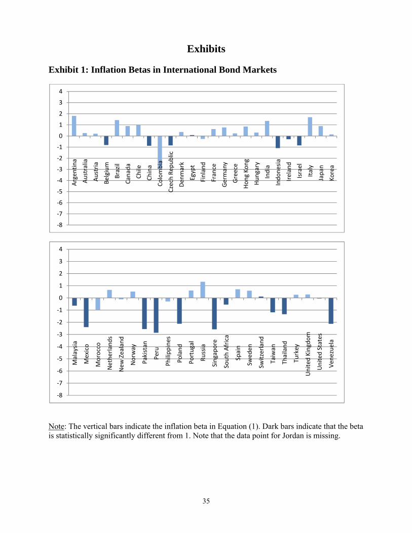
35

Exhibits Exhibit 1: Inflation Betas in International Bond Markets

Note: The vertical bars indicate the inflation beta in Equation (1). Dark bars indicate that the beta is statistically significantly different from 1. Note that the data point for Jordan is missing.

‐8

‐7

‐6

‐5

‐4

‐3

‐2

‐1

0

1

2

3

4

Argen

tina

Australia

Austria

Belgium

Brazil

Canada

Chile

China

Colombia

Czech Rep

ublic

Den

mark

Egypt

Finland

France

Germany

Greece

Hong Kong

Hungary

India

Indonesia

Ireland

Israel

Italy

Japan

Korea

‐8

‐7

‐6

‐5

‐4

‐3

‐2

‐1

0

1

2

3

4

Malaysia

Mexico

Morocco

Netherlands

New

Zealand

Norw

ay

Pakistan

Peru

Philippines

Poland

Portugal

Russia

Singapore

South Africa

Spain

Swed

en

Switzerland

Taiwan

Thailand

Turkey

United

Kingdom

United

States

Ven

ezuela

36

Exhibit 2: Inflation Betas in International Stock Markets

Note: The vertical bars indicate the inflation beta in Equation (1). Dark bars indicate that the beta is statistically significantly different from 1.

‐8

‐7

‐6

‐5

‐4

‐3

‐2

‐1

0

1

2

3

4Argen

tina

Australia

Austria

Belgium

Brazil

Canada

Chile

China

Colombia

Czech Rep

ublic

Den

mark

Egypt

Finland

France

Germany

Greece

Hong Kong

Hungary

India

Indonesia

Ireland

Israel

Italy

Japan

Jordan

Korea

‐8

‐7

‐6

‐5

‐4

‐3

‐2

‐1

0

1

2

3

4

Malaysia

Mexico

Morocco

Netherlands

New

Zealand

Norw

ay

Pakistan

Peru

Philippines

Poland

Portugal

Russia

Singapore

South Africa

Spain

Swed

en

Switzerland

Taiwan

Thailand

Turkey

United

Kingdom

United

States

Ven

ezuela

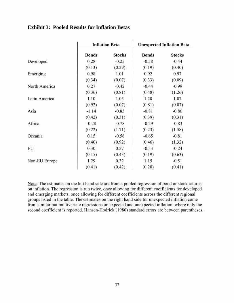
37

Exhibit 3: Pooled Results for Inflation Betas Inflation Beta Unexpected Inflation Beta

Bonds Stocks Bonds Stocks Developed 0.28

(0.13) -0.25 (0.29)

-0.58 (0.19)

-0.44 (0.40)

Emerging 0.98 (0.34)

1.01 (0.07)

0.92 (0.33)

0.97 (0.09)

North America 0.27 (0.36)

-0.42 (0.81)

-0.44 (0.48)

-0.99 (1.26)

Latin America 1.10 (0.92)

1.05 (0.07)

1.20 (0.81)

1.07 (0.07)

Asia -1.14 (0.42)

-0.83 (0.31)

-0.81 (0.39)

-0.86 (0.31)

Africa -0.28 (0.22)

-0.78 (1.71)

-0.29 (0.23)

-0.83 (1.58)

Oceania 0.15 (0.40)

-0.56 (0.92)

-0.65 (0.46)

-0.81 (1.32)

EU 0.30 (0.15)

0.27 (0.43)

-0.53 (0.19)

-0.24 (0.63)

Non-EU Europe 1.29 (0.41)

0.32 (0.42)

1.15 (0.20)

-0.51 (0.41)

Note: The estimates on the left hand side are from a pooled regression of bond or stock returns on inflation. The regression is run twice, once allowing for different coefficients for developed and emerging markets; once allowing for different coefficients across the different regional groups listed in the table. The estimates on the right hand side for unexpected inflation come from similar but multivariate regressions on expected and unexpected inflation, where only the second coefficient is reported. Hansen-Hodrick (1980) standard errors are between parentheses.

38

Exhibit 4: Inflation Betas over Longer Horizons Bonds Stocks

1-Year

Horizon 2-Year

Horizon 3-Year

Horizon 4-Year

Horizon 5-Year

Horizon 1-Year

Horizon 2-Year

Horizon 3-Year

Horizon 4-Year

Horizon 5-Year

Horizon

Developed countries

0.28 (0.13)

0.59 (0.15)

0.84 (0.17)

1.04 (0.18)

1.12 (0.19)

-0.25 (0.29)

-0.11 (0.27)

-0.05 (0.25)

0.01 (0.23)

0.12 (0.23)

Emerging countries

0.98 (0.34)

1.63 (0.34)

2.02 (0.52)

1.21 (0.57)

2.11 (0.65)

1.01 (0.07)

1.02 (0.03)

1.03 (0.03)

1.03 (0.03)

1.00 (0.03)

North America

0.27 (0.36)

0.67 (0.21)

1.04 (0.30)

1.13 (0.32)

1.39 (0.45)

-0.42 (0.81)

-0.40 (0.69)

-0.31 (0.59)

-0.25 (0.51)

-0.16 (0.45)

European Union

0.30 (0.15)

0.65 (0.19)

0.94 (0.23)

1.11 (0.23)

1.17 (0.23)

0.27 (0.43)

-0.09 (0.35)

-0.05 (0.32)

-0.10 (0.29)

-0.04 (0.28)

Note: We repeat the pooled regressions from Exhibit 3 but also perform them over longer multi-year horizons, up till 5 years. The standard errors correct for the overlap in the observations using Hansen-Hodrick (1980) standard errors.

Exhibit 5: Unexpected Inflation Betas over Longer Horizons

Bonds Stocks

1-Year

Horizon 2-Year

Horizon 3-Year

Horizon 4-Year

Horizon 5-Year

Horizon 1-Year

Horizon 2-Year

Horizon 3-Year

Horizon 4-Year

Horizon 5-Year

Horizon

Developed countries

-0.58 (0.19)

-0.58 (0.15)

-0.22 (0.13)

0.19 (0.13)

0.36 (0.13)

-0.44 (0.40)

-0.59 (0.32)

-0.59 (0.33)

-0.66 (0.34)

-0.58 (0.31)

Emerging countries

0.92 (0.33)

1.57 (0.37)

1.93 (0.54)

1.08 (0.58)

2.09 (0.68)

0.97 (0.09)

0.98 (0.05)

1.03 (0.03)

1.04 (0.03)

1.03 (0.04)

North America

-0.44 (0.48)

-0.62 (0.33)

0.07 (0.19)

0.26 (0.31)

0.47 (0.34)

-0.99 (1.26)

-1.08 (0.90)

-0.74 (0.69)

-0.75 (0.55)

-0.84 (0.41)

European Union

-0.53 (0.19)

-0.43 (0.17)

-0.09 (0.17)

0.23 (0.17)

0.44 (0.16)

-0.24 (0.63)

-0.92 (0.54)

-1.26 (0.43)

-1.39 (0.36)

-1.21 (0.30)

Note: We repeat the pooled regressions from Exhibit 3 but also perform them over longer multi-year horizons, up till 5 years. The standard errors correct for the overlap in the observations using Hansen-Hodrick (1980) standard errors.

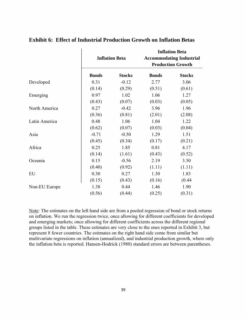
39

Exhibit 6: Effect of Industrial Production Growth on Inflation Betas

Inflation Beta Inflation Beta

Accommodating Industrial Production Growth

Bonds Stocks Bonds Stocks Developed 0.31

(0.14) -0.12 (0.29)

2.77 (0.51)

3.06 (0.61)


1.02 (0.07)

1.06 (0.03)

1.27 (0.05)


-0.42 (0.81)

3.96 (2.01)

1.96 (2.08)


1.06 (0.07)

1.04 (0.03)

1.22 (0.04)

Asia -0.71 (0.45)

-0.50 (0.34)

1.29 (0.17)

1.51 (0.21)

Africa 0.25 (0.14)

1.85 (1.61)

0.81 (0.43)

4.17 (0.52)

Oceania 0.15 (0.40)

-0.56 (0.92)

2.19 (1.11)

3.50 (1.11)

EU 0.30 (0.15)

0.27 (0.43)

1.30 (0.16)

1.83 (0.44

Non-EU Europe 1.38 (0.56)

0.44 (0.44)

1.46 (0.25)

1.90 (0.31)

Note: The estimates on the left hand side are from a pooled regression of bond or stock returns on inflation. We run the regression twice, once allowing for different coefficients for developed and emerging markets; once allowing for different coefficients across the different regional groups listed in the table. These estimates are very close to the ones reported in Exhibit 3, but represent 8 fewer countries. The estimates on the right hand side come from similar but multivariate regressions on inflation (annualized), and industrial production growth, where only the inflation beta is reported. Hansen-Hodrick (1980) standard errors are between parentheses.

40

Exhibit 7: Inflation Betas for Other Asset Classes

Inflation Beta Unexpected Inflation Beta

Foreign Bonds

Real Estate

Gold Gold Futures

Foreign Bonds

Real Estate

Gold Gold Futures

Developed 1.65 (0.62)

-2.46 (0.91)

1.25 (0.40

1.38 (0.49)

1.36 (0.50)

-0.43 (1.01)

2.30 (0.45)

2.36 (0.53)


0.91 (0.03)

0.92 (0.03)

1.06 (0.03)

1.06 (0.03)

1.07 (0.03)


2.04 (4.58)

1.45 (1.67)

1.24 (1.90)

-0.06 (0.91)

2.19 (4.18)

3.96 (2.01)

2.92 (2.17)


0.92 (0.03)

0.92 (0.03)

1.04 (0.03)

1.04 (0.03)

1.04 (0.03)

Asia 1.01 (0.05)

-0.20 (1.05)

0.94 (0.09)

0.93 (0.09)

1.06 (0.09)

1.33 (1.54)

1.29 (0.17)

1.25 (0.17)

Africa 1.16 (0.38)

0.57 (0.43)

0.52 (0.45)

0.98 (0.31)

0.81 (0.43)

0.78 (0.43)

Oceania 1.03 (0.48)

-2.18 (2.47)

1.10 (0.73)

1.29 (0.93)

1.24 (0.52)

-1.93 (2.48)

2.19 (1.11)

2.52 (1.22)

EU 1.20 (0.17)

-4.33 (1.34)

0.99 (0.11)

1.01 (0.11)

1.20 (0.10)

-1.42 (1.36)

1.17 (0.07)

1.18 (0.07)

Non-EU Europe

0.86 (0.17)

-9.52 (3.27)

0.82 (0.16)

0.81 (0.16)

1.48 (0.21)

-8.50 (4.07)

1.46 (0.25)

1.43 (0.25)

Note: The estimates here mimic the univariate regressions of Exhibit 3, but use as the return series an equally weighted major government bond return, a local real estate return, and spot and futures gold returns.

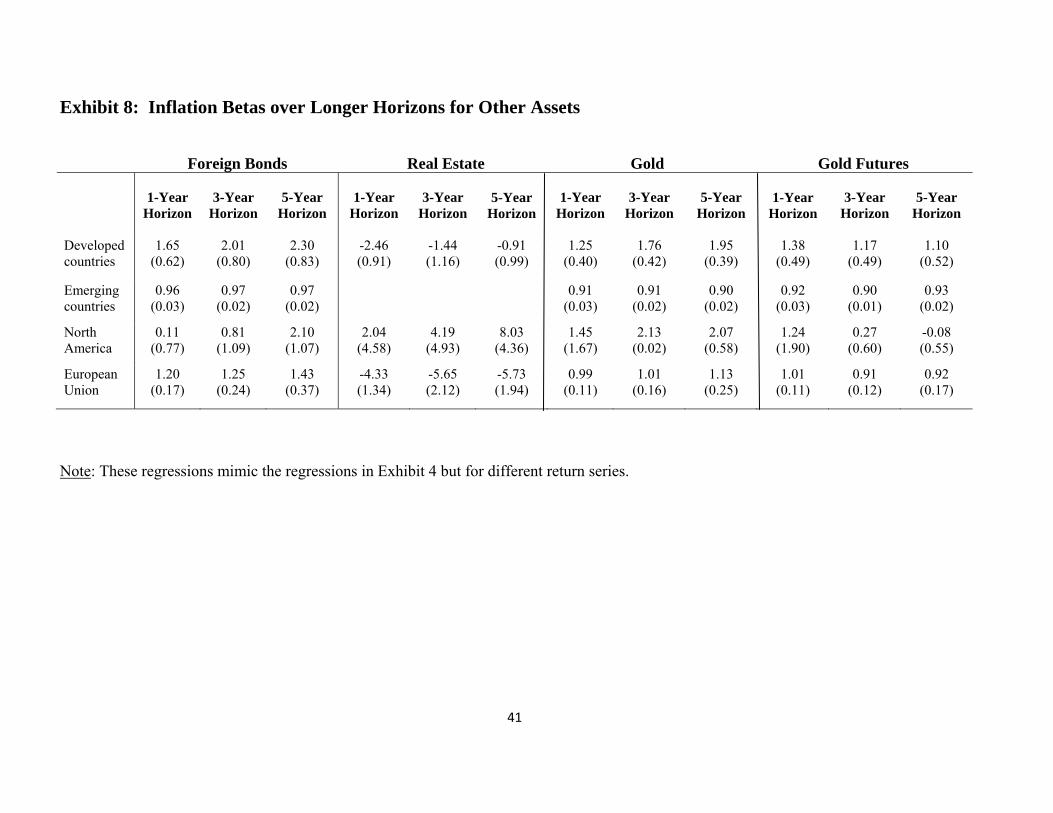
41

Exhibit 8: Inflation Betas over Longer Horizons for Other Assets Foreign Bonds Real Estate Gold Gold Futures

1-Year Horizon

3-Year Horizon

5-Year Horizon

1-Year Horizon

3-Year Horizon

5-Year

Horizon 1-Year

Horizon 3-Year

Horizon 5-Year

Horizon

1-Year

Horizon 3-Year

Horizon 5-Year

Horizon

Developed countries

1.65 (0.62)

2.01 (0.80)

2.30 (0.83)

-2.46 (0.91)

-1.44 (1.16)

-0.91 (0.99)

1.25 (0.40)

1.76 (0.42)

1.95 (0.39)

1.38 (0.49)

1.17 (0.49)

1.10 (0.52)

Emerging countries

0.96 (0.03)

0.97 (0.02)

0.97 (0.02)

0.91 (0.03)

0.91 (0.02)

0.90 (0.02)

0.92 (0.03)

0.90 (0.01)

0.93 (0.02)

North America

0.11 (0.77)

0.81 (1.09)

2.10 (1.07)

2.04 (4.58)

4.19 (4.93)

8.03 (4.36)

1.45 (1.67)

2.13 (0.02)

2.07 (0.58)

1.24 (1.90)

0.27 (0.60)

-0.08 (0.55)

European Union

1.20 (0.17)

1.25 (0.24)

1.43 (0.37)

-4.33 (1.34)

-5.65 (2.12)

-5.73 (1.94)

0.99 (0.11)

1.01 (0.16)

1.13 (0.25)

1.01 (0.11)

0.91 (0.12)

0.92 (0.17)

Note: These regressions mimic the regressions in Exhibit 4 but for different return series.

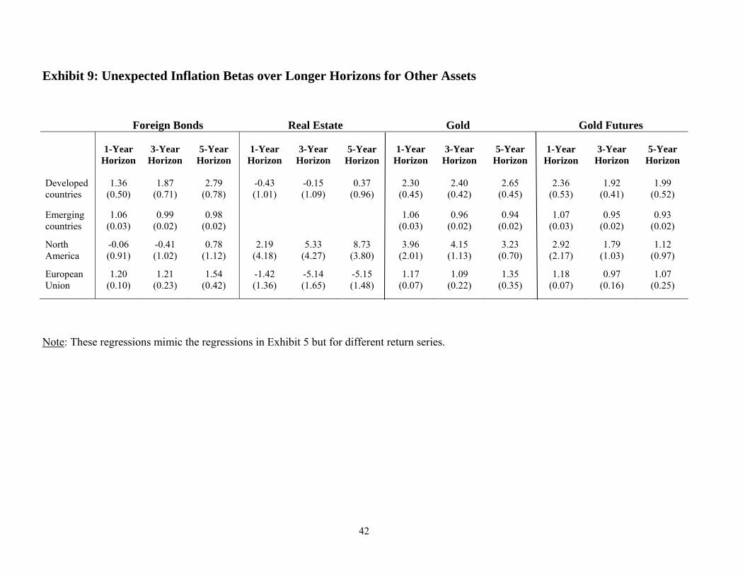
42

Exhibit 9: Unexpected Inflation Betas over Longer Horizons for Other Assets

Foreign Bonds Real Estate Gold Gold Futures

1-Year Horizon

3-Year Horizon

5-Year Horizon

1-Year Horizon

3-Year Horizon

5-Year

Horizon 1-Year

Horizon 3-Year

Horizon 5-Year

Horizon

1-Year

Horizon 3-Year

Horizon 5-Year

Horizon

Developed countries

1.36 (0.50)

1.87 (0.71)

2.79 (0.78)

-0.43 (1.01)

-0.15 (1.09)

0.37 (0.96)

2.30 (0.45)

2.40 (0.42)

2.65 (0.45)

2.36 (0.53)

1.92 (0.41)

1.99 (0.52)

Emerging countries

1.06 (0.03)

0.99 (0.02)

0.98 (0.02)

1.06 (0.03)

0.96 (0.02)

0.94 (0.02)

1.07 (0.03)

0.95 (0.02)

0.93 (0.02)

North America

-0.06 (0.91)

-0.41 (1.02)

0.78 (1.12)

2.19 (4.18)

5.33 (4.27)

8.73 (3.80)

3.96 (2.01)

4.15 (1.13)

3.23 (0.70)

2.92 (2.17)

1.79 (1.03)

1.12 (0.97)

European Union

1.20 (0.10)

1.21 (0.23)

1.54 (0.42)

-1.42 (1.36)

-5.14 (1.65)

-5.15 (1.48)

1.17 (0.07)

1.09 (0.22)

1.35 (0.35)

1.18 (0.07)

0.97 (0.16)

1.07 (0.25)

Note: These regressions mimic the regressions in Exhibit 5 but for different return series.

43

Exhibit 10: Stability of Inflation Betas Panel A: Inflation Betas 1-yr horizon

Bond pre-1990 Bond post-1990 Stock pre-1990 Stock post-1990 Developed 0.60 (0.18) 0.02 (0.17)*** -0.24 (0.30) -1.12 (0.74) Emerging NA 0.98 (0.34) 1.31 (0.04) 0.95 (0.07)*** North America 0.35 (0.45) -0.25 (0.56) -0.55 (0.85) -1.35 (1.48) Latin America NA 1.10 (0.92) 1.30 (0.03) 1.00 (0.07)*** Asia 1.29 (0.92) -1.21 (0.42)** 0.26 (0.62) -1.38 (0.37)** Africa NA -0.28 (0.22) NA -0.73 (1.71) Oceania 0.33 (0.49) 0.01 (0.49) -0.87 (0.89) -3.38 (1.15)** EU 0.74 (0.24) 0.04 (0.18)*** 0.24 (0.38) 0.38 (0.89) Non-EU Europe 0.54 (0.49) 1.30 (0.42) 0.45 (0.54) 0.31 (0.42)

3-yr horizon Bond pre-1990 Bond post-1990 Stock pre-1990 Stock post-1990

Developed 1.35 (0.18) 0.56 (0.17)*** -0.08 (0.26) -0.66 (0.58) Emerging NA 2.02 (0.52) NA 1.03 (0.03) North America 1.17 (0.24) 0.29 (0.51)* -0.68 (0.61) -2.00 (1.13) Latin America NA 0.23 (0.38) NA 1.05 (0.02) Asia 3.31 (0.63) 0.77 (0.17)*** 0.66 (0.41) -0.34 (0.48)* Africa NA -0.52 (0.35) NA 1.88 (2.68) Oceania NA 0.16 (0.54) -0.67 (0.56) -2.90 (1.16)*** EU 1.48 (0.22) 0.67 (0.21)*** -0.02 (0.33) -0.28 (0.58) Non-EU Europe 1.75 (0.65) 2.90 (0.23) -0.18 (0.63) 0.74 (0.25)


Developed 1.67 (0.24) 0.95 (0.17)*** 0.10 (0.23) -0.04 (0.45) Emerging NA 2.11 (0.65) NA 1.00 (0.03) North America 1.93 (0.27) 0.75 (0.36)*** -0.53 (0.41) -1.59 (0.83) Latin America NA 0.31 (0.16) NA 1.02 (0.02) Asia 3.91 (0.92) 0.91 (0.41)*** 1.01 (0.34) 0.05 (0.60)* Africa NA -0.18 (0.55) NA 4.75 (2.09) Oceania NA 0.85 (1.18) 0.16 (0.47) -0.50 (0.53) EU 1.63 (0.27) 1.03 (0.21)*** -0.05 (0.28) -0.32 (0.46) Non-EU Europe 1.92 (0.69) 2.81 (0.33) 0.04 (0.59) 0.82 (0.19)

44

Panel B: Unexpected Inflation Betas 1-yr horizon

Bond pre-1990 Bond post-1990 Stock pre-1990 Stock post-1990 Developed -0.95 (0.32) -0.55 (0.21) -1.34 (0.41) 1.06 (1.00)**

Emerging NA 0.92 (0.33) 1.12 (0.10) 0.88 (0.10)

North America -1.82 (0.82) -0.33 (0.48)* 0.59 (0.34) -2.95 (1.12)**

Latin America NA 1.20 (0.81) NA 1.00 (1.60)

Asia -0.30 (0.58) -0.85 (0.39) 1.17 (0.07) 1.00 (0.08)***

Africa NA -0.29 (0.23) NA 0.33 (0.44)

Oceania -2.78 (1.30) -0.56 (0.46)* -1.43 (0.33) -0.83 (1.58)

EU -0.84 (0.37) -0.53 (0.20)* -1.79 (2.00) -2.39 (1.11)***

Non-EU Europe 0.01 (0.68) 1.17 (0.20)* -1.77 (0.61) 1.85 (1.07)**


Developed 0.69 (0.21) -0.37 (0.15)*** -0.75 (0.38) -0.55 (0.73)

Emerging NA 1.93 (0.54) NA 1.03 (0.03)

North America 0.66 (0.47) -0.30 (0.41) -1.23 (0.70) -0.79 (1.09)


Asia 1.20 (0.33) 0.16 (0.26)*** 0.88 (0.31) -0.27 (0.47)**

Africa NA -0.44 (0.27) NA 1.86 (2.68)

Oceania NA -0.60 (0.18) -1.03 (0.83) -1.90 (0.85)

EU 0.63 (0.25) -0.21 (0.18)*** -1.52 (0.43) -1.10 (0.97)

Non-EU Europe 1.19 (0.54) 2.79 (0.19)*** -1.66 (0.65) 0.58 (0.26)


Developed 1.13 (0.28) 0.32 (0.13)*** -0.73 (0.35) -0.17 (0.61)

Emerging NA 2.09 (0.68) NA 1.03 (0.04)

North America 1.66 (0.43) 0.35 (0.37)*** -1.08 (0.44) -1.09 (0.71)


Asia 3.70 (0.48) 0.38 (0.30)*** 1.04 (0.39) 0.21 (0.74)

Africa NA -0.15 (0.27) NA 4.84 (2.03)

Oceania NA -0.08 (0.57) -0.64 (0.56) -0.14 (0.52)

EU 0.98 (0.35) 0.41 (0.16) -1.52 (0.29) -1.11 (0.71)

Non-EU Europe 1.54 (0.79) 2.83 (0.29) -0.80 (0.63) 0.80 (0.23) Note: The estimates in Panel A are from a pooled regression of bond or stock returns on inflation. We run the regression twice, once allowing for different coefficients for developed and emerging markets; once allowing for different coefficients across the different regional groups listed in the table. The estimates for Panel B come from similar but multivariate regressions on expected and unexpected inflation, where only the second coefficient is reported. Standard errors are between parentheses. The regressions are run splitting the sample in 1990. The asterisk after the second column indicates whether a test for parameter stability rejects at the 10% (*), 5% (**) or 1% (***) level. NA indicates that there were no data for that part of the sample and/or that country group.

Exhibit 11: Stability of Inflation Betas in the US

45

Panel A: Inflation Betas

Bonds Stocks Break Date Pre Beta Post Beta Pre Beta Post Beta

1973 -0.28 (1.25)

-0.74 (0.41)

-3.03 (2.49)

-0.74 (0.82)

1980 -0.04 (0.53)

-0.66 (0.53)

-1.60 (1.02)

0.19 (1.02)

1990 -0.50 (0.46)

-0.18 (1.45)

-1.02 (0.85)

-1.51 (2.73)

2000 -0.52 (0.42)

-0.27 (1.87)

-1.30 (0.74)

2.23 (3.39)

Panel B: Unexpected Inflation Betas


1973 -3.80 (0.72)

-2.07 (0.51)

-7.66 (3.84)

-2.78 (1.14)

1980 -1.00 (0.71)

-2.96** (0.66)

-4.83 (1.56)

-0.93* (1.43)

1990 -2.28 (0.61)

-0.93 (1.23)

-3.68 (1.26)

-1.57 (2.53)

2000 -2.38 (0.57)

-0.28 (1.65)

-3.98 (1.11)

2.05* (3.20)

Panel C: Inflation Betas Accommodating Industrial Production Growth Exposure


1973 -0.81 (1.29)

-0.92 (0.40)

-3.17 (2.58)

-0.55 (0.80)

1980 -0.16 (0.55)

-0.98 (0.51)

-1.61 (1.04)

0.64 (0.97)

1990 -1.08 (0.45)

-0.42 (1.32)

-1.28 (0.80)

0.05 (2.39)

2000 -1.06 (0.41)

0.46 (1.74)

-1.56 (0.72)

-1.35 (3.23)

Note: We use data on bond and stock returns for the US starting in January 1960 to the end of 2008. We consider 4 different break dates for the (unexpected) inflation betas reported on the left; when a multivariate regression is run, all coefficients are allowed to break. The asterisk after the second column indicates whether a test for parameter stability rejects at the 10% (*), 5% (**) or 1% (***) level. We report the beta pre- and post-break.

46

Exhibit 12: Tracking Inflation

Panel A: Constrained Weights

Stocks Bonds Foreign Bonds

Real Estate Gold Spot

All 0.055 0.608 0.217 -0.009 0.136

Developed 0.033 0.816 -0.006 -0.009 0.166

Emerging 0.075 0.417 0.414 n/a 0.110

North America 0.078 0.681 0.054 0.015 0.171

Latin America 0.166 0.184 0.675 n/a -0.024

Asia 0.049 0.551 0.269 -0.030 0.177

Africa 0.029 0.360 0.510 n/a 0.101

Oceania 0.091 0.827 -0.089 0.030 0.142

EU 0.007 0.836 -0.009 -0.005 0.170

Non-EU Europe 0.082 0.611 0.206 -0.069 0.135

Panel B: Constrained Weights, Including T-Bills

Stocks Bonds Foreign Bond

Real Estate Gold Spot T-Bills

All -0.013 -0.063 0.032 0.009 0.058 1.001 Developed -0.005 -0.017 -0.020 0.009 0.062 0.971

Emerging -0.020 -0.104 0.078 n/a 0.054 1.028

North America 0.003 -0.015 -0.006 0.027 0.075 0.917

Latin America -0.032 -0.071 0.114 n/a 0.007 0.982

Asia -0.018 -0.134 0.009 -0.018 0.065 1.156

Africa -0.044 -0.188 0.212 n/a -0.003 1.024

Oceania -0.011 -0.161 -0.026 0.018 0.095 1.084

EU -0.010 -0.044 -0.031 0.012 0.059 1.015

Non-EU Europe 0.038 0.222 0.150 0.006 0.133 0.455

Panel C: Unconstrained Weights

Stocks Bonds Foreign Bond

Real Estate Gold Spot T-Bills R2

All -0.017 -0.064 0.037 -0.005 0.010 -0.165 0.486 Developed -0.004 -0.025 -0.003 -0.005 0.010 0.136 0.347

Emerging -0.028 -0.101 0.073 n/a 0.010 -0.442 0.609

North America -0.004 0.007 -0.020 0.009 0.011 0.231 0.248

Latin America -0.032 -0.079 0.093 n/a 0.006 -0.281 0.695

Asia -0.017 -0.068 0.017 -0.025 0.043 0.923 0.614

Africa -0.043 -0.272 0.190 n/a -0.022 -6.355 0.470

Oceania -0.034 -0.068 -0.022 0.003 0.040 -0.274 0.457

EU -0.007 -0.045 -0.005 -0.002 -0.003 0.062 0.319

Non-EU Europe -0.008 0.011 0.135 -0.015 -0.031 0.035 0.531

Note: For each country, we find the portfolio weights that minimize the squared tracking error with inflation and then aggregate these weights over various country groups. In Panels A and B, the weights sum to 1; in Panel C, they are unconstrained.

47

Exhibit 13: TIPS: Assets under Management and Outstanding Amount

Source: Taken from Graph 3 in Roush, Dudley and Ezer and (2008).

48

Exhibit 14: Properties of the Inflation Risk Premium in the US Inflation Regimes

QTRS 1 2 Unconditional

1 -0.01 (0.01)

-0.01 (0.00)

-0.01 (0.01)

4 0.34 (0.11)

-0.14 (0.07)

0.31 (0.10)

12 0.98 (0.30)

0.12 (0.18)

0.91 (0.28)

20 1.19 (0.37)

0.48 (0.26)

1.14 (0.36)

[normal] [disinflation]

Source: Ang, Bekaert and Wei (2008).

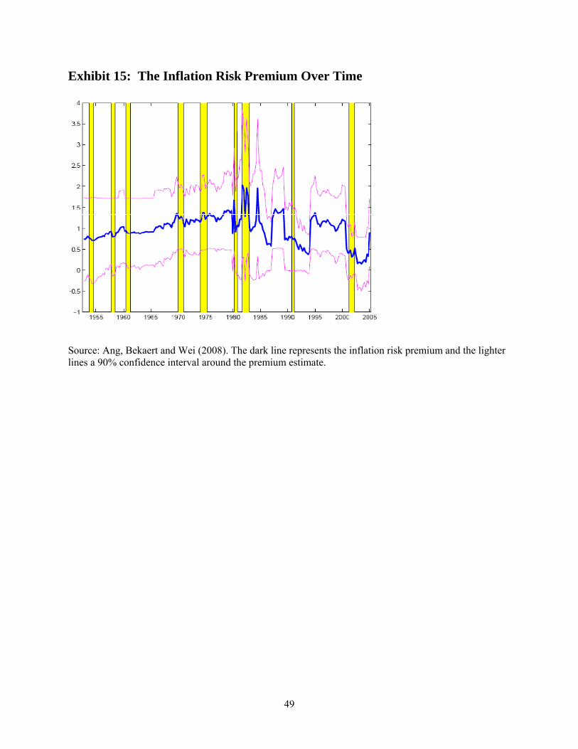
49

Exhibit 15: The Inflation Risk Premium Over Time

Source: Ang, Bekaert and Wei (2008). The dark line represents the inflation risk premium and the lighter lines a 90% confidence interval around the premium estimate.

50

Exhibit 16: Treasury Volume in the TIPS Market

Source: Taken from Roush, Dudley, and Ezer (2008), Graph 2, Average Daily Secondary Market Trading Volume in TIPS. They used a 12 week moving average of the actual data.

51

Exhibit 17: The Illiquidity Premium in the 10-Year TIPS Yield

Source: D’Amico, Kim and Wei (2008).

Percent

52

Exhibit 18: Recent Inflation Risk Premium Estimates

US Euro UK

Maturity in years

HPR* DKW CM GH CLR HT GW R JLS

1 NA 35 19 NA NA NA 7 174 NA

5 27 36 NA 25 -5 25 25 184 [0,200]

10 51 64 216 50 -5 0 NA 173 NA

20 82 NA NA NA NA NA NA NA NA

30 101 NA NA NA NA NA NA NA NA

TIPS X X X X

TIPS Problem X X

Surveys X X X X X

Notes: Full references for the studies mentioned here can be found in the reference list. The line TIPS indicates that TIPS were used, but only in “liquid” periods. The line “TIPS Problem” refers to the fact that TIPS were used without accounting for the liquidity premium. The line “Surveys” indicates that survey forecasts were used to help identify expected inflation. *They do not use TIPS data but use inflation swap rates from 2003 onward.

Inflation Risk and the Inflation Risk Premium*

Documents