1 Location management and Moving Objects Databases Ouri Wolfson University of Illinois, Chicago [email protected]

Welcome message from author
This document is posted to help you gain knowledge. Please leave a comment to let me know what you think about it! Share it to your friends and learn new things together.
Transcript

1
Location management and Moving Objects Databases
Ouri WolfsonUniversity of Illinois, Chicago
2
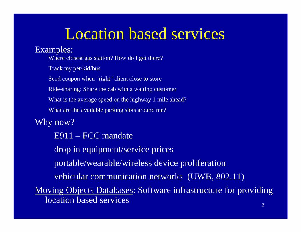
Location based servicesExamples:
Where closest gas station? How do I get there?
Track my pet/kid/bus
Send coupon when "right" client close to store
Ride-sharing: Share the cab with a waiting customer
What is the average speed on the highway 1 mile ahead?
What are the available parking slots around me?
Why now?E911 – FCC mandatedrop in equipment/service pricesportable/wearable/wireless device proliferationvehicular communication networks (UWB, 802.11)
Moving Objects Databases: Software infrastructure for providing location based services

3
Spatial information Temporal informationMoving objects databases
Location management
4
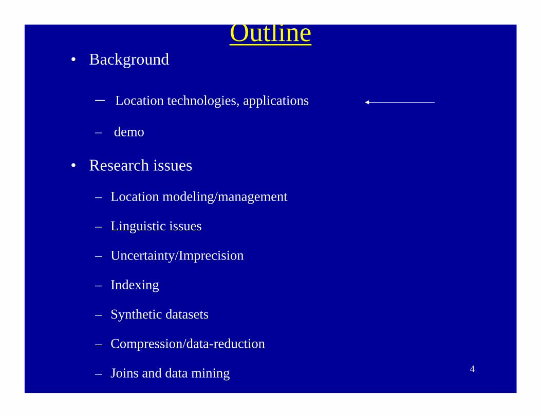
Outline• Background
– Location technologies, applications
– demo
• Research issues
– Location modeling/management
– Linguistic issues
– Uncertainty/Imprecision
– Indexing
– Synthetic datasets
– Compression/data-reduction
– Joins and data mining

5
Fundamental location sensing methods
• Triangulation
• Proximity
• Scene analysis – camera location + shape/size/direction of object ==>
object location)

6
Location/Positioning technologies
• Global Positioning System (GPS) – Special purpose computer chip– cost < $100– As small as a cm²– Receives and triangulates signals from 24
satellites at 20,000 KM– Computes latitude and longitude with tennis-
court-size precision – Used to be football field until May 1st, 2000;
US stopped jamming of signal for civilian use. Same devices will work.
– Differential GPS: 2-3 feet precision

7
Location technologies (continued)
• Indoor (sonar) GPS• Sensors – e.g. toll booth that detects card in
windshield.• Triangulation in cellular architecture • Cell-id• Bluetooth (proximity positioning)• calendar system

8
Moving Objects Database Technology
Query/trigger examples:• During the past year, how many times was bus#5 late by more than 10
minutes at station 20, or at some station (past query)• Send me message when helicopter in a given geographic area (trigger)• Trucks that will reach destination within 20 minutes (future query)• Taxi cabs within 1 mile of my location (present query)• Average speed on highway, one mile ahead • Tracking for “context awareness”
GPS
GPS
GPS
Wireless link
9
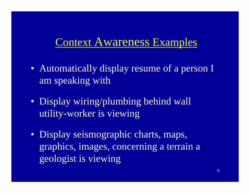
Context Awareness Examples
• Automatically display resume of a person I am speaking with
• Display wiring/plumbing behind wall utility-worker is viewing
• Display seismographic charts, maps, graphics, images, concerning a terrain a geologist is viewing

10
Importance of Tracking Accuracy
Server errs by > R-r Disturbs real time
Example:

11
Mobile e-commerce
• Remind me to buy drinks when I’m close to a supermarket
• Send a coupon (10% off) to a customer with interest in Nike sneakers that is close to the store
• Inform a person entering a bar of his “buddies” in the bar

12
Mobile e-commerce
• Alert a person entering a bar if two of his “buddies” (wife and girlfriend) are both in the bar; he may want to turn around
• Antithesis of e-commerce, which is independent of location.

13
Applications-- Summary• Geographic resource discovery-- e.g. “Closest gas station”• Digital Battlefield• Transportation (taxi, courier, emergency response, municipal
transportation, traffic control)• Supply Chain Management, logistics• Context-awareness, augmented-reality, fly-through visualization• Location- or Mobile-Ecommerce and Marketing• Mobile workforce management• Air traffic control (www.faa.gov/freeflight)• Dynamic allocation of bandwidth in cellular network• Querying in mobile environments
Currently built in an ad hoc fashion

14
Outline• Background
– Location technologies, applications
– demo
• Research issues
– Location modeling/management
– Linguistic issues
– Uncertainty/Imprecision
– Indexing
– Synthetic datasets
– Compression/data-reduction
– Joins and data mining

15
Outline (continued)
– Querying in mobile environments

16
• Envelope software on top of a Database Management System and a Geographic Information System.
• Platform for Location-based-services application development.
Demo at ACM-SIGMOD’99, NGITS’99, ICDE’00
Moving Objects Database Architecture
Moving Objects S/W GIS
DBMS

17
Query result showing all vehicle’s locations at 12:35

18
Which vehicle will be closest to the “star” between 12:35 and 12:50?

19
Answer: The vehicle on the red route

20
When will each vehicle enter the specified sector?

21
Routes prior to overlaying current traffic conditions

22
Real-time traffic showing delays on east/west road

23
Impact of traffic slows down vehicle on red route

24
Outline• Background
– Location technologies, applications
– demo
• Research issues
– Location modeling/management
– Uncertainty/Imprecision
– Linguistic issues
– Indexing
– Synthetic datasets
– Compression/data-reduction
– Joins and data mining

25
Location modeling/management
• In the cellular architecture (network location management)
• In Moving Objects Databases (geographic location management)
26
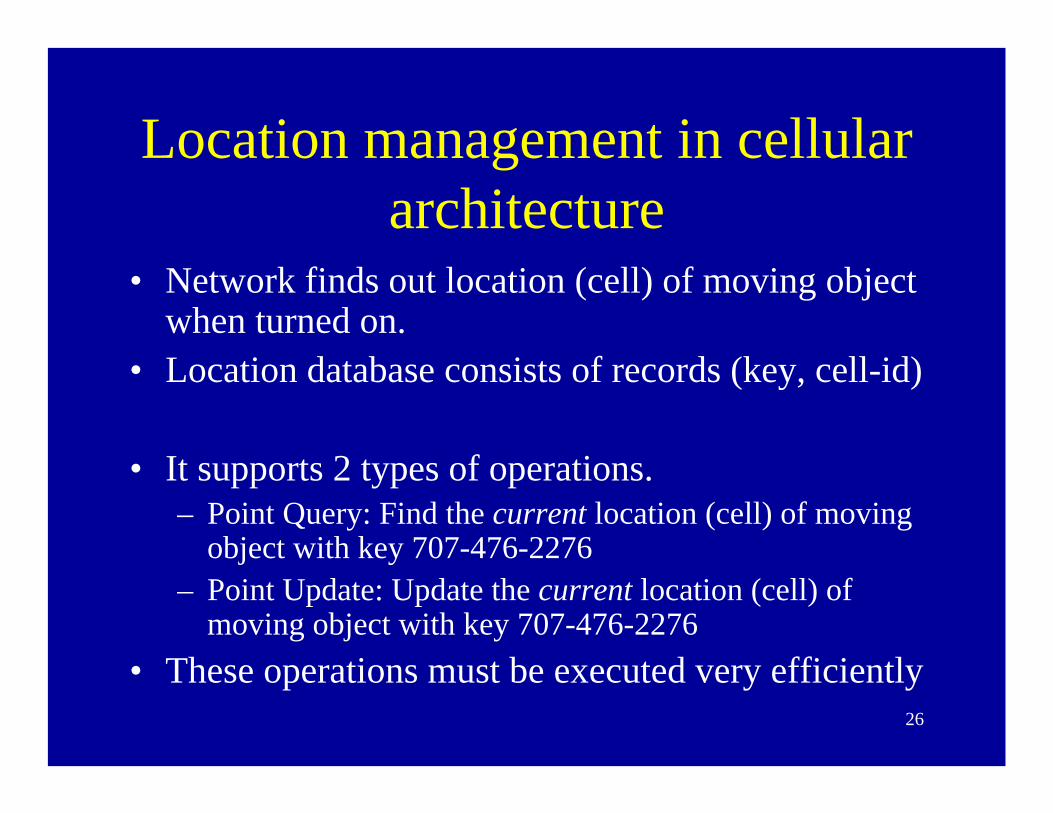
Location management in cellular architecture
• Network finds out location (cell) of moving object when turned on.
• Location database consists of records (key, cell-id)
• It supports 2 types of operations.– Point Query: Find the current location (cell) of moving
object with key 707-476-2276– Point Update: Update the current location (cell) of
moving object with key 707-476-2276• These operations must be executed very efficiently
27
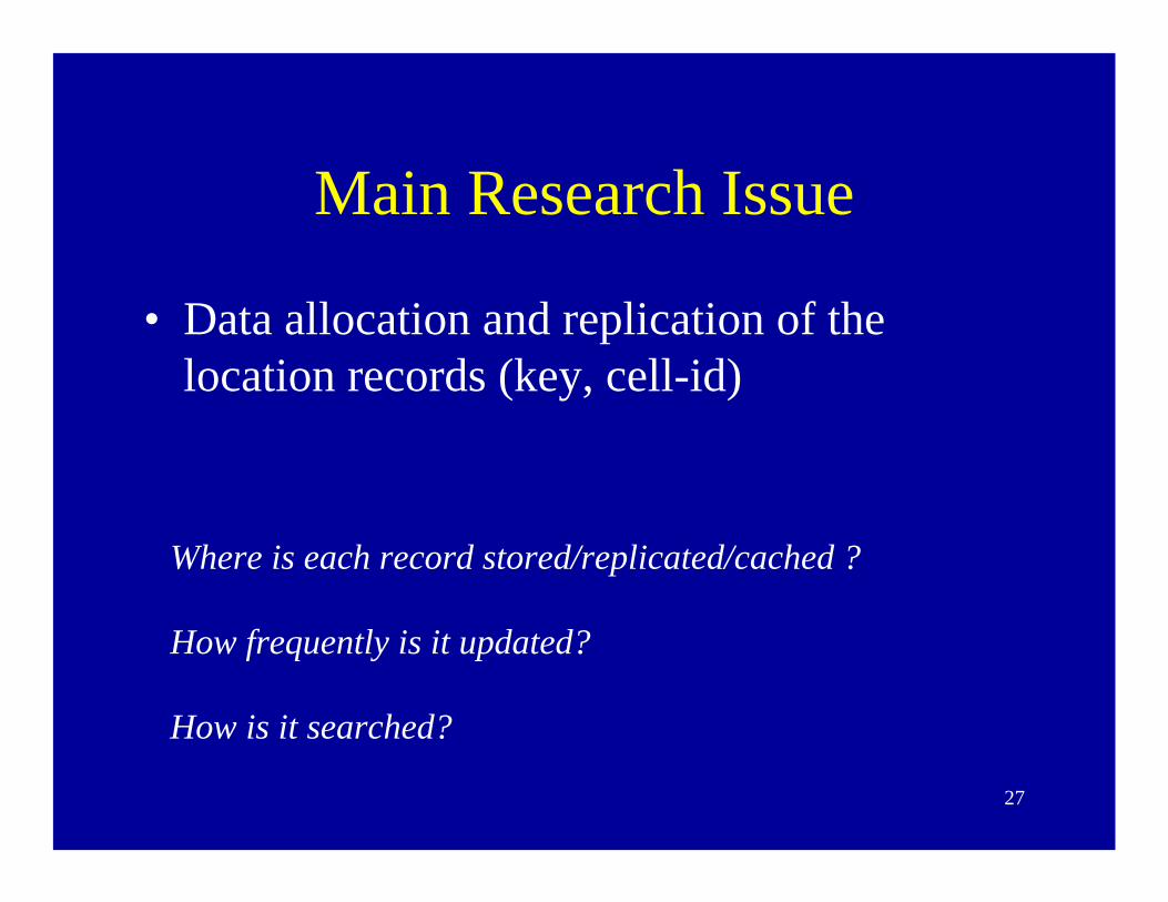
Main Research Issue
• Data allocation and replication of the location records (key, cell-id)
Where is each record stored/replicated/cached ?
How frequently is it updated?
How is it searched?

28
Cellular Architecture
support stationMSS
Mobile
Moving Object
Moving Object
support stationMSS
Moving Object
Mobile
Moving Object
Moving Object
Moving Object
support stationMSS
Mobile
Moving Object
Moving Object
Wireless linkWireless link
Cell size ranges from 0.5 to several miles in diameter in Cell size ranges from 0.5 to several miles in diameter in wideareawidearea terrestrial networksterrestrial networks
Moving Object

29
Some naïve solutions• Centralized database: all location records reside
at a central location. – Drawback: Remote lookup for every call, and remote
update for every cell crossing.• Fully replicated: all location records are replicated
at each MSS.– Drawback: for every cell crossing the database at every
MSS has to be updated.• Partitioned: each MSS keeps a database of the
moving objects in its cell– Drawback: for every remote call the database at each
MSS has to be queried.

30
Hierarchical Solution
• When a moves from 1 to 2 LA database is updated, but not central database.
• A call that originates in 2 needs to search only the LA database.• This scheme exploits the locality of calls and moves.• Can obviously be generalized to arbitrary number of levels.• Call execution uses a different network.
Central Databasea - A
Location Area Aa - 1
MSSMSSMSS
a
1 2 3

31
Variant• Partition the centralized database
a - k s - zl - r
LA
MSS
LA LA
MSS MSS MSS MSS MSS MSS MSS

32
European and North American Standard• Notion of home location• Partition centralized database based on home location of
subscribers
LA
MSS MSS MSS
HLRVLR
HLRVLR
LA
MSS MSS MSS
Home Location Register – Profile and MSS of local subscriberVisitor Location Register – MSS of visitor in LAMove – Update HLR to point to new MSS or foreign VLR, or update VLRy call x – Check local VLR of y, if not found check HLR of x

33
Variant
• Don’t update on local cellular move, only LA move• Call: Page in LA• Database update activity is reduced at the expense of paging activity.• Useful for users that move a lot, but do not get many calls.• Paging overhead can be further reduced by prediction
LA
MSS
LA LA
MSS MSS MSS MSS MSS
No update Update

34
Variant
• Cache in LA database the MSS of remote users called recently
LA
MSS
LA LA
MSS MSS MSS MSS MSS MSS MSS

35
Other Variants• Designate some cells as reporting cells
(moving objects must update upon entering them); calls processed by paging neighborhood of last reporting cell
• Distance/movement/time-based updates
rrr
r r r

36
Other Variants (continued)
• Data mining and prediction mechanisms to reduce location-update traffic and compensate for this by a smart search/paging on calls.
• Objective: tradeoff between search and update overhead to balance total load
• Comprehensive survey: Pitoura & Samaras 99

37
Geolocation management
• Why is it different?• Higher resolution
Joe, pick up a customer in cell 75 ! --doesn’t work since diameter may be > 3 miles
• Interested in past and future location• Variety of queries

38
Model of a trajectory for geolocationmanagement
Y
X
Time
Present time
2d-ROUTE
3d-TRAJECTORY
Approximation: does not capture acceleration/deceleration
Point Objects: modelneeds to be extended for objects with extent, eg, hurricanes

39
Trajectory Construction - example
• Based on GPS points (x1,y1,t1), (x2,y2,t2),…
• For vehicles moving on road networks, construction uses a map.

40
Map• A relation
tuple <----> block, i.e. section of street between two intersections
… …
… …
… …
… …
… …
864
906
728
312
R_f_add
891No25A31HALSTED167981
782No25A40CABRINI167985
398No25A40ARTHINGTON167980
956
R_t_addpolyline
No
one_way
A31
category
25HALSTED167982
Avgspeednamebid
A region taken from the map of Chicago

41
Past-trajectory construction
• Based on GPS points (x1,y1,t1), (x2,y2,t2),…• “Snap” points on road network
• Find shortest path on map between consecutive gps points

42
Future-trajectory construction
• Client informs location server of: – start-time of trip– start-location– destination(s)
• Server finds shortest path on a map
• Converts path into a trajectory using drive-time attribute

43
Enables Prediction
• Time-travel queriese.g. Where will object X be in 10 mins?

44
Trajectory Poly-line as Current-Location attribute
• Similar to Location attribute for static objects
• DBMS provides an abstraction of the trajectory data – Dynamic Attribute
• Value of Dynamic Attribute continuously changes as time progresses
• Vast implications for query processing -- open research problem
• Moreover: Dynamic Attribute should account for uncertainty.
45
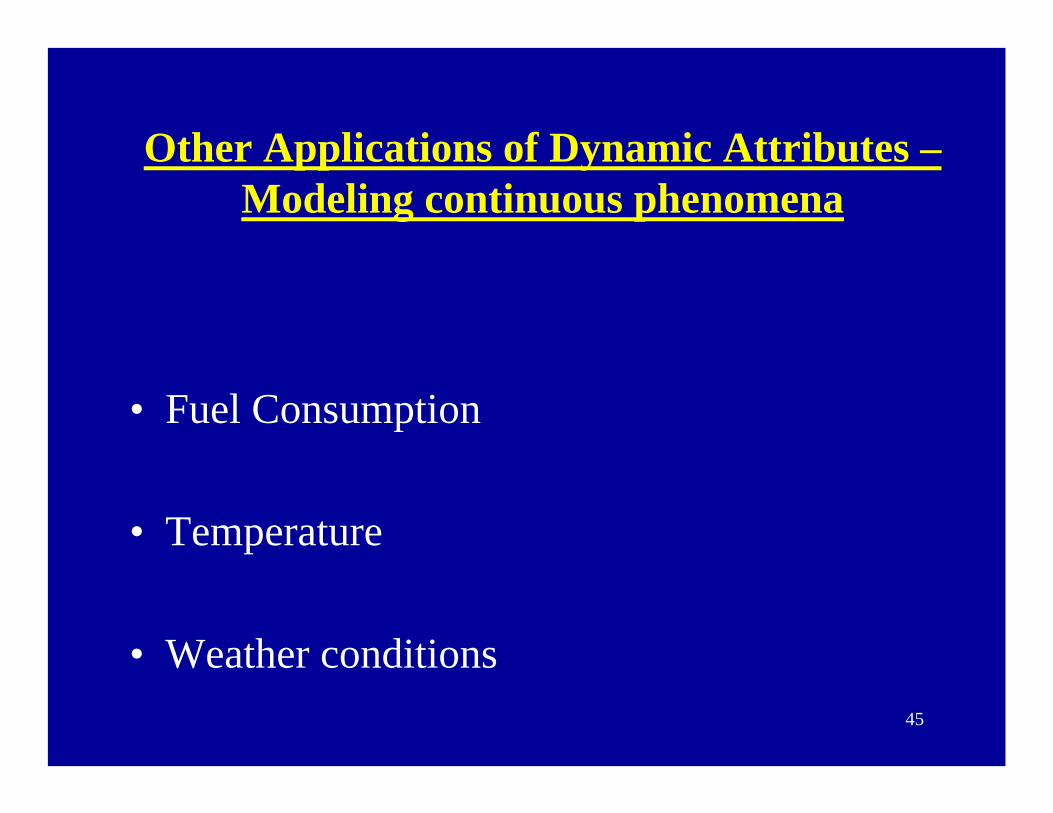
Other Applications of Dynamic Attributes –Modeling continuous phenomena
• Fuel Consumption
• Temperature
• Weather conditions

46
Traffic effects

47
Trajectory Modification
Y
X
Time
Present time
2d-ROUTE
3d-TRAJECTORY
Heavy traffic
OW2

Slide 47
OW2 before present time: completed motion.after present time: expected motionOuri Wolfson, 7/23/2003

48
Traffic information sourcesLoop sensors
Probe vehicles

49
Trajectory update involves speed prediction
Y
X
Time
Present time
2d-ROUTE
3d-TRAJECTORY
Heavy traffic
x

50
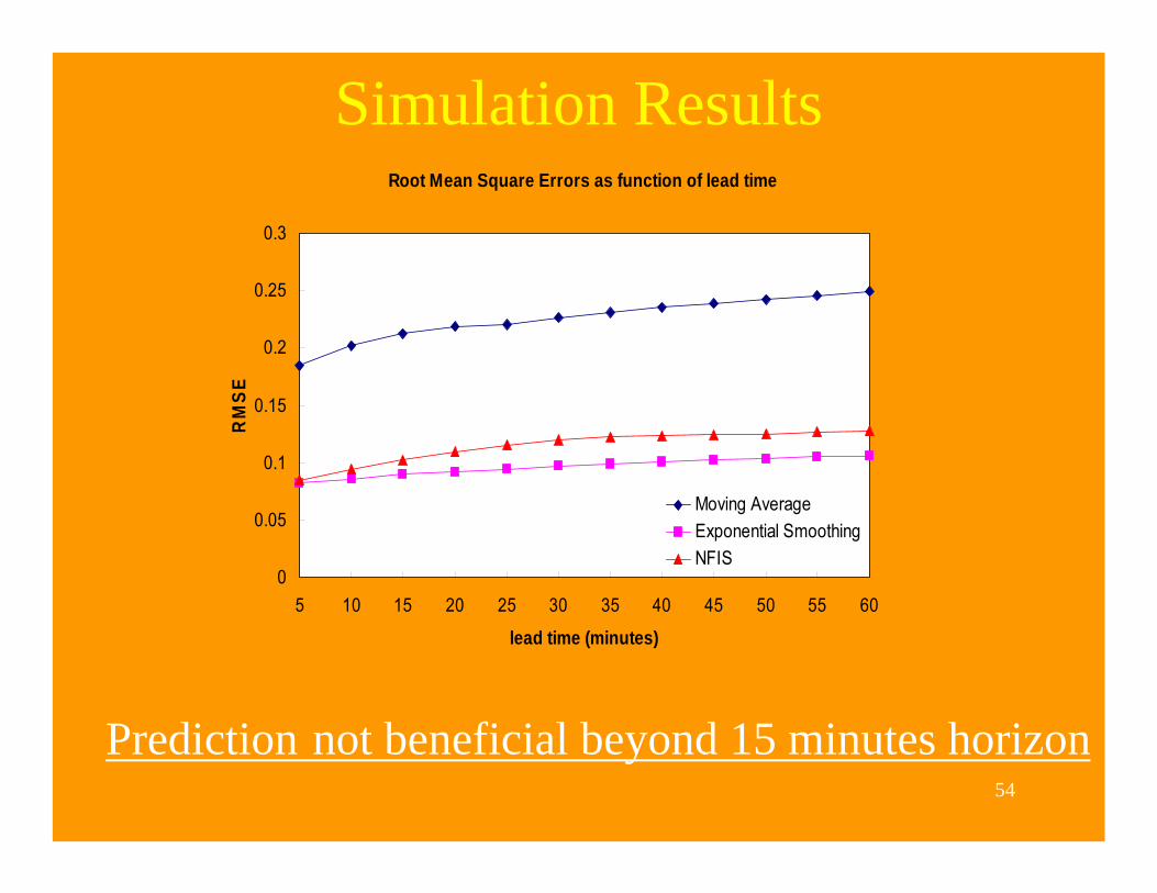
Problem 1: Speed (time series) prediction
• performance of different time-series prediction methods

51
Three Time-series Prediction Methods
• Two widely used methods:– Moving Averages: the next predicted value is the average
of the latest h values of the series– Exponential Smoothing: The next predicted value is the
weighted average of the latest h values, and the weights decrease geometrically with the age of the values
• Neural-Fuzzy Inference Systems (NFIS)– Fuzzy rule based inference +– Neural back-propagation rule base learning

52
Comparison by Experiments

53
Experimental Environment
• Real speed time-series collected on the EdensExpressway in Chicago
• Speed data collected for each of the 72 blocks every 5 minutes for 20 days
54
Simulation ResultsRoot Mean Square Errors as function of lead time
0
0.05
0.1
0.15
0.2
0.25
0.3
5 10 15 20 25 30 35 40 45 50 55 60
lead time (minutes)
RM
SE
Moving AverageExponential SmoothingNFIS
Prediction not beneficial beyond 15 minutes horizon

55
Problem 2: Avoid continuous trajectory revision
• Solution idea: filter + refinement at query time

56
Traffic prediction references:[1] J. S. R. Jang, C. T. Sun, and E. Mizutani. .Neuro-Fuzzy and Soft Computing. Prentice-Hall, 1997.[2] D.~C. Montgomery, L.~A. Johnson, and J.~S. Gardiner. Forecasting and Time Series Analysis.
McGraw-Hill, 1990. [3] Y. Ohra, T. Koyama, and S. Shimada. Online-learning type of traveling time prediction model in
expressway. In Proc. of IEEE Conf. on Intelligent Transportation System, pages 350--355, Nov. 1997.[4] H. Dia. An object-oriented neural network approach to short-term traffic forecasting. European Journal
of Operational Research, 131:253--261, 2001.[5] J. Anderson and M.~Bell. Travel time estimation in urban road networks. In Proc. of IEEE Conf. on
Intelligent Transportation System, pages 924--929, Nov. 1997.[6] G. Trajcevski, O. Wolfson, and B. Xu. Real-time traffic updates in moving objects database. In the Fifth
International Workshop on Mobility in Databases and Distributed Systems, September 2002.[7] L. Chen and F. Y. Wang. A neuro-fuzzy system approach for forecasting short-term freeway traffic
flows. In Proceedings of the IEEE 5th International Conference on Intelligent Transportation Systems, September 2002.
[8] S. Pallottino and M. G. Scutella. Shortest path algorithms in transportation models: classical and innovative aspects. In Equilibrium and Advanced Transportation Modeling, Kluwer (1998) 245-281.
[9] J. Kwon, B. Coifman, and P.~J. Bickel. Day-to-day travel time trends and travel time prediction from loop detector data. In Transportation Research Record, number 1712, pages 120--129, 2000.
[10] G. Das, K. Lin, H. Mannila, G. Renganathan, and P. Smyth. Rule discovery from time series. In KDD98, pages 16--22, 1998.

57
Location Modeling References[1] A. Prasad Sistla, Ouri Wolfson, Sam Chamberlain and Son Dao, Modeling and Querying Moving Objects, In Proceedings of the 13th International Conference on Data Engineering, p422-432, April 7-11, 1997 Birmingham U.K. IEEE Computer Society 1997.
[2] Evaggelia Pitoura and George Samaras, Locating Objects in Mobile Computing, Knowledge and Data Engineering, vol13, no.4, p571-592, 2001.
[3] Amiya Bhattacharya and Sajal K. Das, LeZi-Update: An Information-Theoretic Approach to Track Mobile Users In PCS Networks, In the proceedings of the 5th Annual ACM/IEEE International Conference on Mobile Computing andNetworking, p1-12, 1999.

58
Outline• Background
– Location technologies, applications
– demo
• Research issues
– Location modeling/management
– Linguistic issues
– Uncertainty/Imprecision
– Indexing
– Synthetic datasets
– Compression/data-reduction
– Joins and data mining

59
Spatio-temporal query/trigger languages
• Relational-oriented (Vazirgiannis and Wolfson 2001)
• Moving Objects Algebra (Gueting et. al. 98-2001)
• Future Temporal Language (Sistla, Wolfson 1997)
• Constraint Query Language (MoktarMoktar, Su, Ibarra 2000) , Su, Ibarra 2000)
60
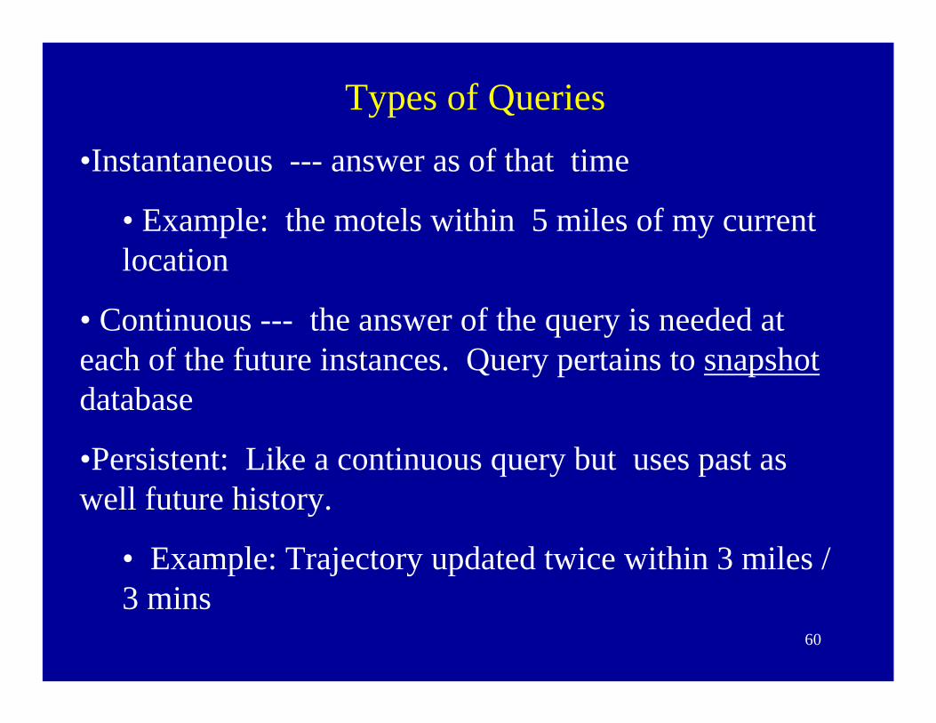
Types of Queries•Instantaneous --- answer as of that time
• Example: the motels within 5 miles of my current location
• Continuous --- the answer of the query is needed at each of the future instances. Query pertains to snapshotdatabase
•Persistent: Like a continuous query but uses past as well future history.
• Example: Trajectory updated twice within 3 miles / 3 mins
61
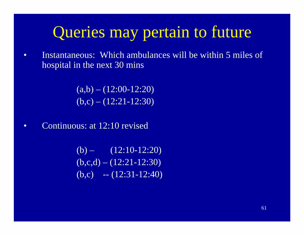
Queries may pertain to future• Instantaneous: Which ambulances will be within 5 miles of
hospital in the next 30 mins
(a,b) – (12:00-12:20)(b,c) – (12:21-12:30)
• Continuous: at 12:10 revised
(b) – (12:10-12:20)(b,c,d) – (12:21-12:30)(b,c) -- (12:31-12:40)

62
Relational Oriented• Point queries:
– where is object 75 at 5pm
– when was object 75 at location (x,y)
• Range queries – temporal constructs– spatial constructs– processing of queries
• Join queries: Retrieve the objects that come within 3 miles of each other at some time-point
63
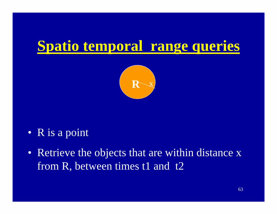
Spatio temporal range queries
R
• R is a point
• Retrieve the objects that are within distance x from R, between times t1 and t2
x
64
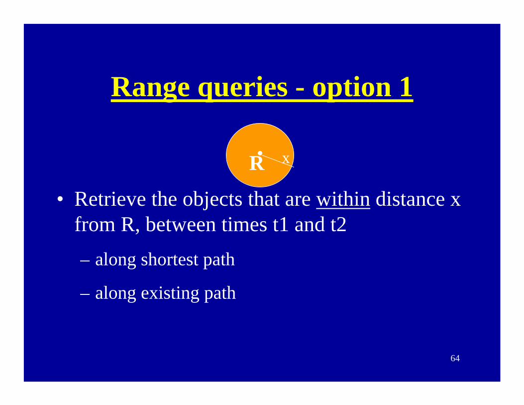
Range queries - option 1
R
• Retrieve the objects that are within distance x from R, between times t1 and t2 – along shortest path
– along existing path
x

65
Range queries - option 1
R
• Retrieve the objects that are within distance x from R, between times t1 and t2 – along shortest path (police patrol vehicles)
xtrajectory
m

66
Range queries - option 1
• Retrieve the objects that are within distance x from R, between times t1 and t2– along existing path (bus)
xtrajectory mR

67
Range queries - option 2
R
• Retrieve the objects that are within distance x from R, between times t1 and t2
• Cost metric– travel time
– travel distance
x
68
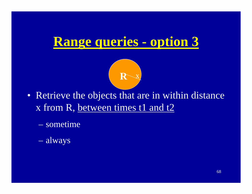
Range queries - option 3
R
• Retrieve the objects that are in within distance x from R, between times t1 and t2– sometime
– always
x

69
Range queries - option 3
R
• objects that are within distance x from R, sometime between times t1 and t2
trajectoryt1
t2

70
Range queries - option 3
R
• objects that are within distance x from R, always between times t1 and t2
trajectoryt1
t2

71
Range queries: 8 options • R on object’s-route within travel-time 5 sometime between
[t1,t2]• R on object’s-route within travel-distance 5 sometime
between [t1,t2]• R on object’s-route within travel-time 5 always between
[t1,t2]• R on object’s-route within travel-distance 5 always in
[t1,t2]
• R within travel-time 5 sometime between [t1,t2]• R within travel-distance 5 sometime between [t1,t2]• R within travel-time 5 always between [t1,t2]• R within travel-distance 5 always between [t1,t2]
72
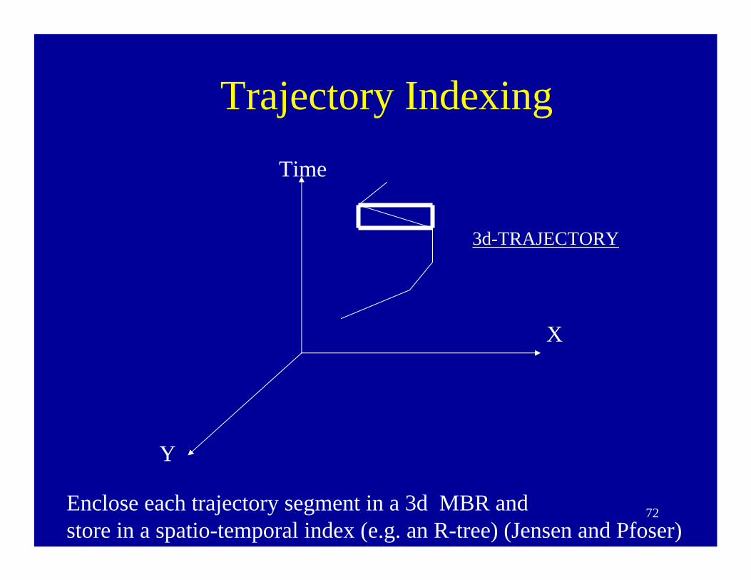
Trajectory Indexing
Y
X
Time
3d-TRAJECTORY
Enclose each trajectory segment in a 3d MBR and store in a spatio-temporal index (e.g. an R-tree) (Jensen and Pfoser)

73
Query Processing Strategy
• Filter -- represent a query as a geometric object Q, and retrieve all the rectangles of the spatio-temporal index which intersect Q
• Refinement -- Check for each trajectory that is stored in a retrieved rectangle whether it satisfies the query.
• Processing methods differ significantly

74
R on Route, within Distance 5, Sometime[t1,t2]
TimeFilter:Q
5
5t2
t1
R
X
Y
S = set of trajectories that are at aerial distance 5 sometime [t1,t2]Refinement:
For each trajectory in S, Check that R is on the red route section.
route
t2
t1
5

75
R on Route, within Distance 5, Always[t1,t2]
TimeFilter Stage:Q
5 5
t2
t1
R
X
Y
S = set of trajectories that are at aerial distance 5 sometime [t1,t2]Refinement:
1) P := all route segments within distance 5 from R (using shortest path on map).
2) For each trajectory in S check whether all route segments traversed during [t1,t2] are in P.
R

76
R on Route, within Travel-time 5, Sometime[t1,t2]
TimeFilter:
Q
t1
t2
R
X
Y
S = Trajectories in index blocks that intersect Q.
Refinement:
For each trajectory in S check that it crosses R sometime during interval [t1, t2 + 5](there may be a trajectory of S that does not intersect R) .
t2 +5

77
Moving Objects Algebra Gueting et. al.Guting et al proposed a rich framework of abstract data-types and a query language for moving objects.
• Moving objects can be points or regions.
• Kernel(Spatial) algebra lifted to the time domain.
• The Kernel consists of spatial types such as points, lines, regions, and different spatial operators, aggregate operators.
• LIFTING: For each type T, a moving type mT.
mT is a function with real time line as the domain and with range of type T.

78
Guetting et al (cont…)
Examples – a moving region a moving pointt
x
t
x
y

79
Gueting et. al. Continued---
•Kernel Operators• Spatial Operators/functions --- INSIDE, TOUCHES, OVERLAPS, DISTANCE.
•Aggregations : min, max, center, etc.
•Distance and Direction operators
•Temporal Operators --- Projection on time domain,
When, atinstant and Rate of change operations etc.

80
Examples
Flight (airline:string, no:int, from:string, to:string,
trajectory:mpoint )
What is the distance traveled by flight LH287 over France?LET trajectory287 = ELEMENT(SELECT trajectory FROM flight WHERE airline = “LH” and no = 257);
length(intersection(France, route(trajectory287)))
81
Examples for Lifting (1)
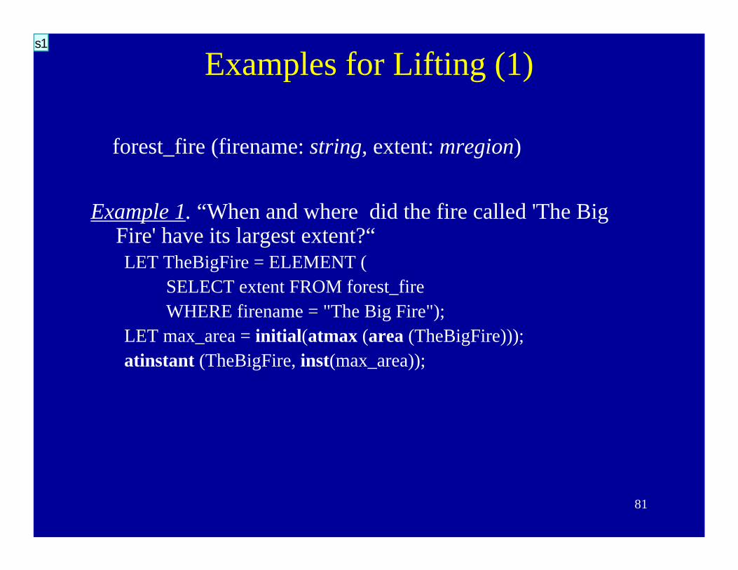
Example 1. “When and where did the fire called 'The Big Fire' have its largest extent?“LET TheBigFire = ELEMENT (
SELECT extent FROM forest_fireWHERE firename = "The Big Fire");
LET max_area = initial(atmax (area (TheBigFire))); atinstant (TheBigFire, inst(max_area));
forest_fire (firename: string, extent: mregion)
s1

Slide 81
s1 Relations "forest", "forest_fire" & "fire_fighter" are used in the examples of lifting.
The relation "forest" records the location and the development of different forests growing and shrinking over time through clearing, cultivation, and destruction processes, for example.
The relation "forest_fire" documents the evolution of different fires from their ignition up to their extinction.
The relation "fire_fighter" describes the motion of fire fighters being on duty from their start at the fire station up to their return.
Example 1: extent is a moving region.TheBigFire is the name of this extent.area in second Let statement is a functionof time. atmax defines pairs (time, area) when the area is maximum, and initial takes the first one.so the second Let statement defines max_area to be a pair (time,value).inst takes the 1st member of the pair (when) and atinstant gives the value of the moving region TheBigFire at that time, i.e. Where the polygon with the max area.
The area operator is used in its lifted version.
Operation atinstant restricts a moving entity to a given instant.
Operation inst returns the time of max_area.
ssss, 7/21/2003

82
Examples for Lifting (2)
• Example 3. "When and where was the spread of fires larger than 500 km2?“
• LET big_part = SELECT big_area AS extent when [FUN (r:region) area(r)>500]FROM forest_fire;
A6

Slide 82
A6 The domain function deftime returnsthe times for which a function is defined.
The second subquery reduces the moving region of each fire to the parts when it was large. For some fires this may never be the case, and hence for them big_area may be empty (always undefined). These are eliminated in the second subquery.Administrator, 1/8/2003
83
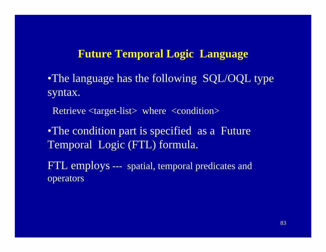
Future Temporal Logic Language
•The language has the following SQL/OQL type syntax.
Retrieve <target-list> where <condition>
•The condition part is specified as a Future Temporal Logic (FTL) formula.
FTL employs --- spatial, temporal predicates and operators

84
FTL --- Continued
•Spatial Operators/predicates :
INSIDE(O,P), DISTANCE(O1,O2)<=5, etc.
•Temporal Operators::Eventually-within-C, Eventually-within-[C,D], f Until g,
Always-for-C, etc.
• Variables and assignment operators

85
Examples•RETRIEVE O.name WHERE
O.color = red and Eventually-within-10 (INSIDE(O,P))
Retrieve names of red color objects that will be inside the region P within 10 units of time.
•RETRIEVE O.name WHERE
Always-for-5 (DISTANCE(O,O’)<=10) and O’.type=truck
Retrieve names of objects that will be within a distance of 10 from a truck for the next five units of time.

86
Examples Contd---
• Retrieve all objects that enter a tunnel in the next 5 units
of time and stay inside it for the subsequent 10 time units.
RETRIEVE O.type WHERE
Not Inside(O,P) and Eventually-within-5(Always-for-10 (Inside(O,P)) and P.type=tunnel
Semantics:FTL formulas are interpreted over future histories specifying the object locations.
Static attributes remain unchanged
Dynamic attributes change according to their functions.

87
Processing Algorithm
The algorithm works inductively on the structure of the FTL formula.
•For atomic formulas p: Answer(p) is obtained using indexing and other traditional methods.
•If p = (p1 and p2 ) or (p1 Until p2) or Eventually-within-C(p1): Answer(p) is computed from Answer(p1) and Answer(p2) inductively.

88
CQL extensions (cont…)
•• Moktar, Su and Ibarra (PODSMoktar, Su and Ibarra (PODS’’00) 00) –– A query language based on the ideas of constraint databases and CQL
Constraint data model: Attribute > 5
(in contrast to the relational model in which Attribute=5)

89
Other Models and Languages - MSI’00 (cont…)
•• Example:Example: Constraint-based representation of 3D motion of an airplane:
30
20
10
5 10 15 20time (min)
height (in 1000m)
ttxttx
ttx
≤∧+−=∨≤≤∧+−=∨
≤≤∧+=
20920010002012252002000
120180001200
25

90
MSI’00 (cont…)
Example: Find all the aircrafts entering Santa Barbara County between t1 and t2
Retrieve y such that:Retrieve y such that:y is an objecty is an object AND AND
there exists a point xthere exists a point x on on traj(ytraj(y)) at time t, at time t, t between t1 and t2,t between t1 and t2, AND AND
x is x is inin Santa Barbara County AND Santa Barbara County AND for every time tfor every time t’’<t the point of <t the point of traj(ytraj(y) at time t) at time t’’ is NOT in SBCis NOT in SBC

91
Languages References[1] A. Prasad Sistla, Ouri Wolfson, Sam Chamberlain and Son Dao, Modeling and Querying Moving Objects, In the proceedings of ICDE, p422-432, 1997.[2] R. Guting, M. Bohlen, M. Erwig, C. Jensen, Lorentzos N, M. Schneider, and M. Vazirgianis. A foundation for representing and querying moving objects. Technical Report 238, FerUniversitat das Hagen (Germany), 1998.[3] M. Vazirgiannis and O. Wolfson, A Spatiotemporal Query Language for Moving Objects, In the proceedings of the conference on Spatial and Temporal Databases, Los Angeles, CA, July 2001.[4] Hoda Mokhtar, Jianwen Su and Oscar Ibarra, On Moving Object Queries, In Proceedings of the 21st ACM SIGMOD-SIGACT-SIGART symposium on Principles of database systems, June 2002.

92
Outline• Background
– Location technologies, applications
– demo
• Research issues
– Location modeling/management
– Linguistic issues
– Uncertainty/Imprecision
– Indexing
– Synthetic datasets
– Compression/data-reduction
– Joins and data mining

93
Where are we?
94
Relationship to location update policies
Linguistic Issues

95
Assumptions set 1• No location prediction provided by human
(e.g. cellular user)
• Fixed location-uncertainty tolerated
• Fixed amount of resources (b/w, processing) for location updates
Power of automatic predictions?

96
Distance Update Policy
• Update when distance of current location from database location > x (uncertainty x)
– Bound on error of answer to query
97
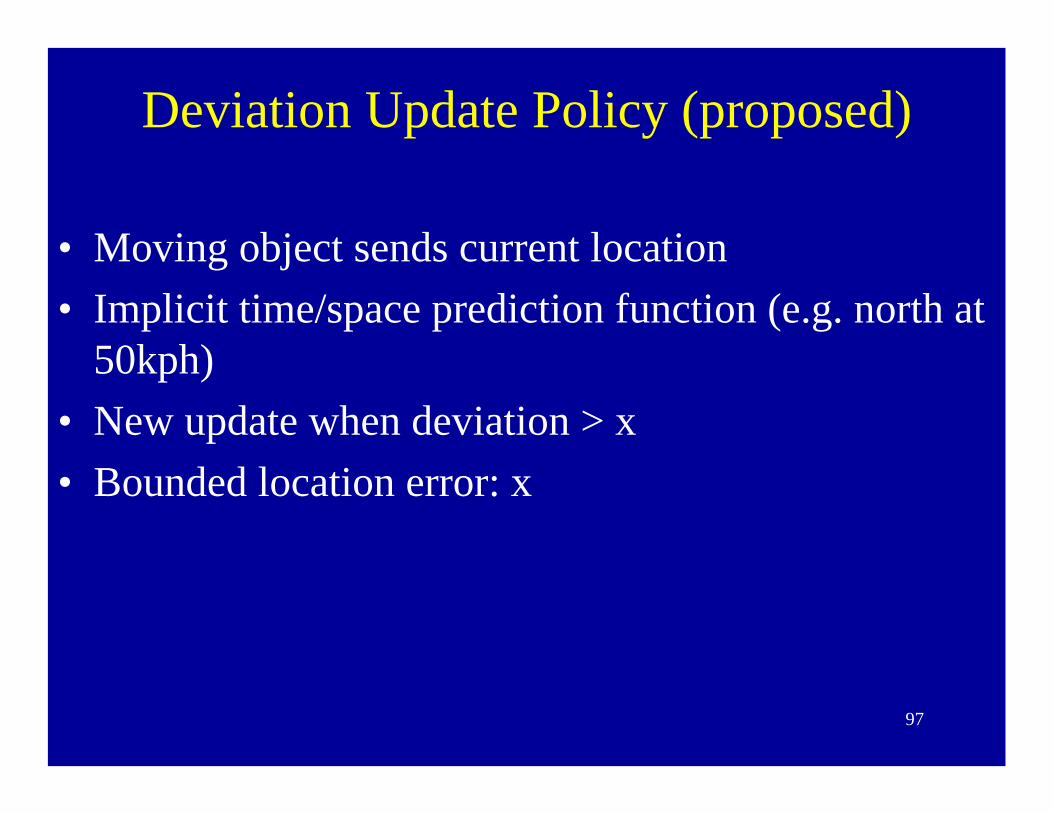
Deviation Update Policy (proposed)
• Moving object sends current location • Implicit time/space prediction function (e.g. north at
50kph)• New update when deviation > x• Bounded location error: x

98
Our Prediction
With average speed since last update
Continues on current street

99
Experimental Results – Euclidean Distance
The number of updates per mile with th = 0.05 − 5.0
0
0.2
0.4
0.6
0.8
1
1.2
1.4
0.7 0.8 0.9 1 1.5 2 5
thnumber of updates per mile
Eu_Deviation_Avg
Eu_Distance
0
2
4
6
8
10
12
14
16
18
0.05 0.1 0.2 0.3 0.4 0.5 0.6
th
number of updates per mile
Eu_Deviation_Avg
Eu_Distance
Up to 40% higher accuracy for a given update capacity

100
Assumptions set 2• No location prediction provided by human
(e.g. cellular user)
• Variable location-uncertainty
• Periodic location updates – automatic toll collection sensors, – heart beat every 30 mins
101
Interpolation
• Pfoster and Jensen ’99.
r1r3
(P1,t1) (P3,t3)
Uncertainty area
Location at time t1<t2<t3 is intersection area of circles wherer1=(t2-t1) • Vmaxr3=(t3-t2) • Vmax

102
Interpolation (continued)
• Uncertainty area between times t1 and t3
(P1,t1) (P3,t3)
ab
Ellipse bounded by the points X such that
X
a + b = Vmax • (t3-t1)
Maximum distance traveled in interval [t1,t3]

103
Assumptions set 3• Future route provided by human
• Variable location-uncertainty
104
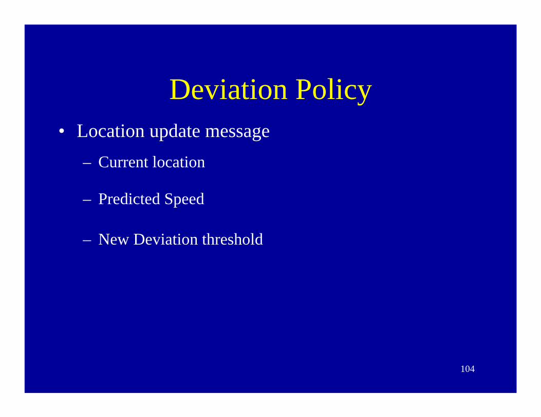
Deviation Policy• Location update message
– Current location
– Predicted Speed
– New Deviation threshold
105
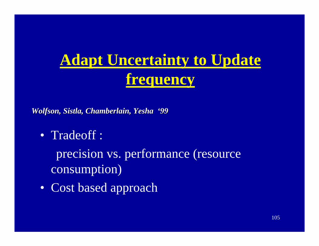
Adapt Uncertainty to Update frequency
• Tradeoff : precision vs. performance (resource
consumption)• Cost based approach
Wolfson, Wolfson, SistlaSistla, Chamberlain, , Chamberlain, YeshaYesha ‘‘9999
106
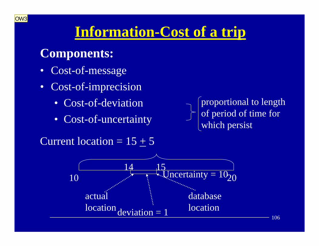
Information-Cost of a tripComponents:• Cost-of-message• Cost-of-imprecision
• Cost-of-deviation • Cost-of-uncertainty
Current location = 15 + 5
proportional to length of period of time for which persist
14
actual location
database locationdeviation = 1
1510 20Uncertainty = 10
OW3

Slide 106
OW3 for a fixed uncertainty, the higher the deviation, the higher the errorOuri Wolfson, 7/23/2003

107
Probability Density Function <-> Imprecision Costs
uncertainty unit cost < deviation unit cost:
uncertainty unit cost > deviation unit cost
Database
location
probability density function
15 2010
probability density function
10 15 20

108
Cost of Deviationunit of deviation
unit of time = 1Cost
∫t2
t1deviation(t)dtCostdeviation(t1,t2) =

109
Cost of Uncertaintyunit of uncertainty
unit of time= CuCost
∫t1
t2 uncertainty(t)dtCostuncertainty(t1,t2) =Cu*

110
Cost of update Message -- Cm
• Cm determined -- how many messages willing to spend to reduce deviation by one, during one time unit
• Cm may vary over time, as a function of load on wireless network
Cm
timet

111
Deviation Threshold Setting by Adaptive Dead Reckoning
predicted deviation
deviation threshold
current timetime
s
Expected total cost - f ( threshold )Theorem: Total cost minimized when:
2 * s * Cm1 + 2 * Cuthreshold =
Wolfson, Jiang, Sistla, Chamberlain, Rishe, Deng; Proc. of the International Conf. on Database Theory, 1999

112
Slope of Predicted Deviation
s s
devi
ati
ond
predicted deviation
current time
time
Approximation of current deviation d by a linear function with same integral as d
113
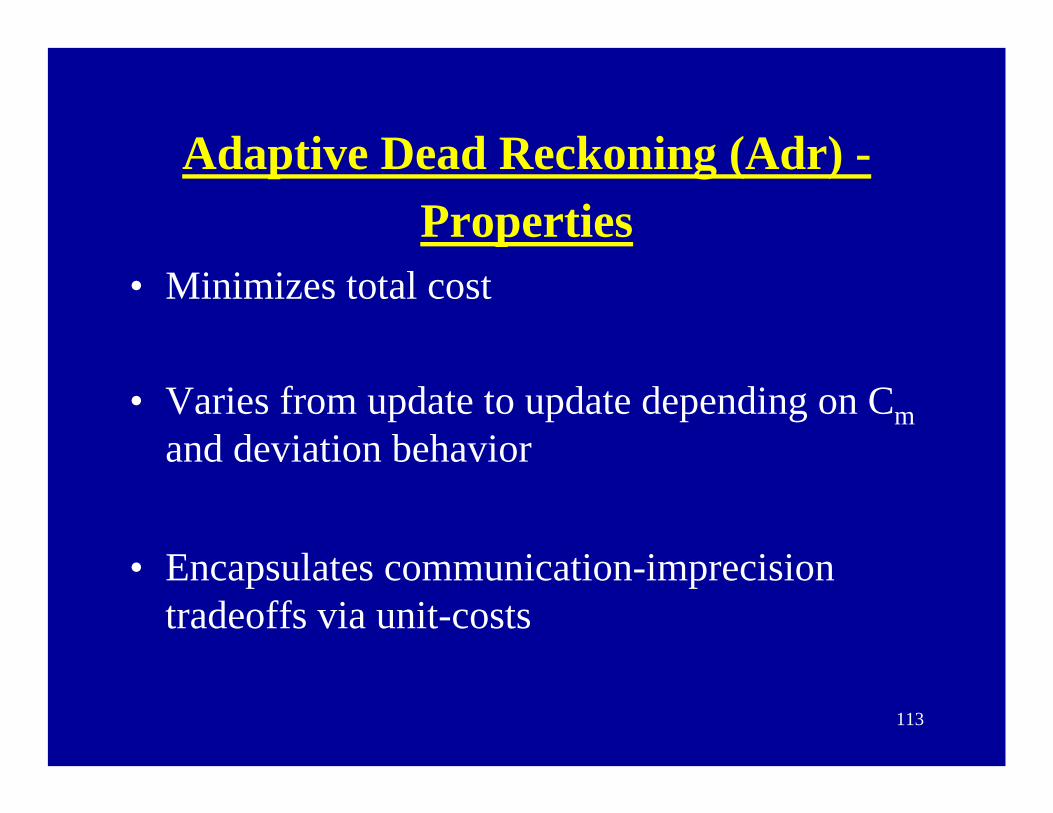
Adaptive Dead Reckoning (Adr) -Properties
• Minimizes total cost
• Varies from update to update depending on Cmand deviation behavior
• Encapsulates communication-imprecision tradeoffs via unit-costs

114
Can there exist a better policy?Maybe ...But
Theorem: There does not exist a competitive online dead-reckoning algorithm.
(Algorithm A is competitive if there are α, βsuch that for every speed curve s:
costA(s)≤α*cost (s) +β)optimal offline algorithm
115
Simulation
Adaptive threshold setting vs.
Fixed threshold
Adaptive consistently outperforms fixed (in terms of
cost)

116
Figure 1 Speed Curve for A Two Hour Trip
0
10
20
30
40
50
60
70
80
0 1000 2000 3000 4000 5000 6000 7000
Time(Secs)
Spee
d(M
iles/
hour
)
'speed'
Methodologyuse a set of speed curves
Figure 2 Speed Curve for A Two Hour Trip
0
10
20
30
40
50
60
70
0 1000 2000 3000 4000 5000 6000 7000
Time(Secs)
Spee
d(M
iles/
hour
)
'speed'
Average distance: 82 miles

117
Average Information Cost, UncerCost=0.25
0
500
1000
1500
2000
1 6 11 16 21 26 31 36 41 46
Update Message Cost
Inform
ation Cos
t
'Adaptive''Fixed Threshold 2.5'
Average Information Cost, UncerCost=3.00
0
500
1000
1500
2000
2500
3000
3500
4000
1 6 11 16 21 26 31 36 41 46
Update Message Cost
Inform
ation Cos
t
'Adaptive''Fixed Threshold 1.0'
•1cent/msg, Cm=20 Fixed=$1.35, Adaptive=$0.70
•Distance location update policy – cost many fold higher

118
UncerCost=0.75
0
500
1000
1500
2000
2500
1 6 11 16 21 26 31 36 41 46
Update Message Cost
Inform
ation Cos
t
'Adaptive''Fixed Threshold 2.5'
UncerCost=0.75
0
100
200
300
400
500
600
700
800
1 6 11 16 21 26 31 36 41 46
Update Message Cost
Cos
t of U
pdate Mes
sage
s
'Adaptive''Fixed Threshold 2.5'
UncerCost=0.75
0
200
400
600
800
1000
1200
1400
1600
1 6 11 16 21 26 31 36 41 46
Update Message Cost
Cos
t of U
ncertainty
'Adaptive''Fixed Threshold 2.5'
UncerCost=0.75
0
100
200
300
400
500
600
700
1 6 11 16 21 26 31 36 41 46
Update Message Cost
Cos
t of D
eviatio
n
'Adaptive''Fixed Threshold 2.5'
The fixed threshold policy uses the same number of messages regardless of the message cost, therefore its uncertainty and deviation costs are constant.

119
A simulation test-bed
How many mobile units can be supported for :
• given level of location accuracy
• given % of b/w for location updates

120
Relationship to location update policies
Linguistic Issues

121
Spatial range queries
SELECT oFROM MOVING-OBJECTSWHERE Inside (o, P)
Retrieve the objects that are in P
P

122
Uncertainty operators in spatial range queries
possibly and definitely semantics based onbranching time
SELECT oFROM MOVING-OBJECTSWHERE Possibly/Definitely Inside (o, P)
Pdefinitely
possibly
uncertainty interval

123
Uncertain trajectory model

124
Possible Motion Curve (PMC) and Trajectory Volume (TV)
• PMC is a continuous function from Time to 2D
• TV is theboundary of theset of all the PMCs(resembles a slanted cylinder)

125
Temporal operators in spatial range queries
SELECT oFROM MOVING-OBJECTSWHERE Sometime/Always(10,11)
inside (o, P)
Retrieve the objects that are in P sometime/always between 10 and 11am
P
10 1110 11sometime always

126
Predicates in spatial range queries
Possibly – there exists a possible motion curveDefinitely -- for all possible motion curves
• possibly-sometime = sometime-possibly• possibly-always• always-possibly• definitely-always = always-definitely• definitely-sometime • sometime-definitely

127
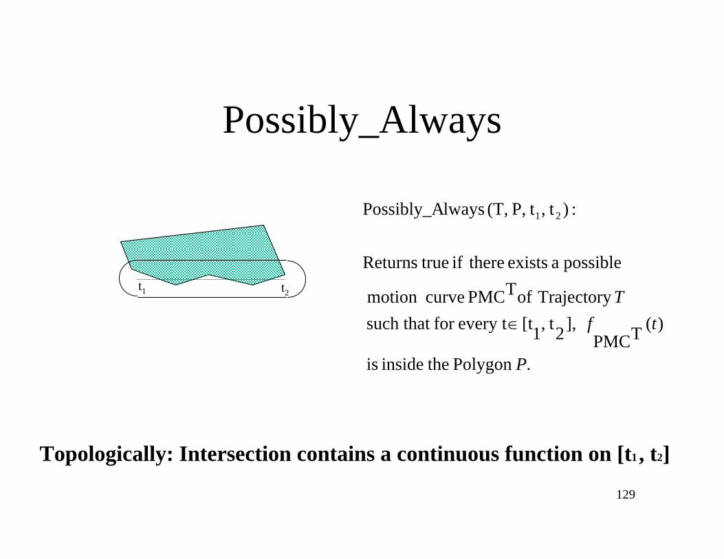
Possibly_Sometime),,,(_ 21 ttPolygonTrajectorySometimePossibly
. Polygon the
inside is that such)(TPMC that
such ]2 t,1[t ta time exists thereand Trajectory ofT PMCcurve motion
possiblea exists There
P
tf
T∈
Topologically:3D:Intersection of prism and trajectory is nonempty2D:Intersection of polygon and trajectory projection is nonempty
128
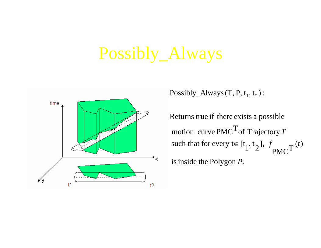
Possibly_Always
.Polygon theinside is
)(TPMC ],2 t,1[tevery tfor such that
Trajectory ofTPMC curvemotion
possible a exists thereif trueReturns
:) t, tP, (T, lwaysPossibly_A 21
P
tfT
∈
Topologically: Intersection contains a continuous function on [t1 , t2]
129
Possibly_Always
t1 t2
.Polygon theinside is
)(TPMC ],2 t,1[tevery tfor such that
Trajectory ofTPMC curvemotion
possible a exists thereif trueReturns
:) t, tP, (T, lwaysPossibly_A 21
P
tfT
∈
Topologically: Intersection contains a continuous function on [t1 , t2]
130
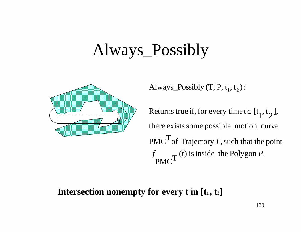
Always_Possibly
t1 t2
.Polygon theinside is)(TPMC
point thesuch that , Trajectory ofTPMC
curvemotion possible some exists there
],2 t,1[t tevery timefor if, trueReturns
:) t, tP, (T,sibly Always_Pos 21
PtfT
∈
Intersection nonempty for every t in [t1 , t2]
131
Definitely_Always
t1 t2
.Polygon the
inside is)(TPMC ],2 t,1[t ttime
every and Trajectory ofTPMC curve
motion possibleevery for if trueReturns
:) t, tP, (T, _AlwaysDefinitely 21
P
tfT
∈
Projection of trajectory contained in polygon

132
Definitely_Sometime
.Polygon theinside
is)(TPMC such that ],2 t,1[t ttime
a exists there, Trajectory ofTPMC curve
motion possibleevery for if, trueReturns
:) t, tP, (T, _SometimeDefinitely 21
P
tfT
∈
Removing the intersection of polygon and trajectory-projection creates more than one connected component

133
Definitely_Sometime
t1 t2
.Polygon theinside
is)(TPMC such that ],2 t,1[t ttime
a exists there, Trajectory ofTPMC curve
motion possibleevery for if, trueReturns
:) t, tP, (T, _SometimeDefinitely 21
P
tfT
∈
Removing the intersection of polygon and trajectory-projection creates more than one connected component

134
Sometime_Definitely
.Polygon the
inside is)(TPMC , Trajectory ofTPMC
curvemotion possibleevery for such that
],2 t,1[t t timea exists thereif, trueReturns
:) t, tP, (T,efinitely Sometime_D 21
P
tfT
∈
The intersection contains an uncertainty area (i.e. a circle with radius = uncertainty threshold)

135
Sometime_Definitely
t1 t2
.Polygon the
inside is)(TPMC , Trajectory ofTPMC
curvemotion possibleevery for such that
],2 t,1[t t timea exists thereif, trueReturns
:) t, tP, (T,efinitely Sometime_D 21
P
tfT
∈
The intersection contains an uncertainty area (i.e. a circle with radius = uncertainty threshold)

136
Relationship among the predicates:
Definitely_Always
Possibly_Always Always_Possibly
Possibly_Sometime
Sometime_Definitely Definitely_Sometime
Theorem: If the query region is convex then Possibly_Always = Always_Possibly. If Circle, alsoSometime_Definitely = Definitely_Sometime

137
PROCESSING RANGE QUERIES=
Filtering using some index (e.g. R-tree or Octree(shown)
+
Refinement (can be done efficiently)

138
Minkowski Sum:

139
Possibly_Sometime

140
Possibly_Always

141
O(n)O(nlogk)O(nk3)Possibly_Always
O(n)O(nlogk)O(nk)Possibly_Sometime
Circular RConvex RConcave ROperator
O(n)O(nlogk + k)O(nk + kkrlogk)Definitely_Always
O(n)O(nlogk + k)O(nk + kkrlogk)Sometime_Definitely
O(n)O(q2nk)O(q2nk + kkrlogk)Definitely_Sometime
O(n)O(nlogk)O(nk)Always_Possibly
Time-complexity summary
a1

Slide 141
a1 n number of straight line segments in trajectoryk number of polygon verticeskr number of reflex verticesq number of intersections between route-segemnts and polygonaa, 4/28/2004

142
Standard deviation depends on :
• time since last update• network reliability
Uncertainty in Language -Quantitative Approach
Uncertainty interval
database location
probability density function

143
Probabilistic Range Queries
SELECT oFROM MOVING-OBJECTSWHERE Inside(o, R)
R
Answer: (RWW850, 0.58)
(ACW930, 0.75)

144
Uncertainty References[1] Ouri Wolfson, Sam Chamberlain, Son Dao, Liqin Jiang and Gisela Mendez, Cost and Imprecision in Modeling the Position of Moving Objects. In Proceedings of the Fourteenth International Conference on Data Engineering, p588-596, February 23-27, 1998, Orlando, Florida, USA. [2] D. Pfoser and C. Jensen, Capturing the uncertainty of Moving Objects Representation. In Proceedings of the 11th International Conference on Scientific and Statistical Databasemanagement, 1999. [3] G. Trajcevski, O. Wolfson, S. Chamberlain and F. Zhang, The Geometry of Uncertainty in Moving Objects Databases, In Proceedings of the 8th Conference on Extending Database Technology (EDBT02), Prague, Czech Republic, March, 2002.[4] G. Trajcevski, O.Wolfson, H.Cao, H.Lin, F.Zhang and N.Rishe, Managing Uncertain Trajectories of Moving Objects with DOMINO. Enterprise Information Systems, Spain, April, 2002.[5] Reynold Cheng, Sunil Prabhakar and Dmitri V. Kalashnikov, Querying imprecise data in moving object environments, In Proc. of the 19th IEEE International Conference on Data Engineering (ICDE 2003), March 5-8, 2003, Bangalore, India.[6] Reynold Cheng, Dmitri V. Kalashnikov and Sunil Prabhakar, Evaluating probabilistic queries over imprecise data, In Proc. of ACM SIGMOD International Conference on Management of Data (SIGMOD’03), June 9-12, 2003, San Diego, CA, USA.

145
Location updates• [1] Ouri Wolfson, A.Prasad Sistla, Sam Chamberlain, and Yelena Yesha, Updating
and Querying Databases that Track Mobile Units. Special issue of the Distributed and Parallel Databases Journal on Mobile Data Management and Applications, 7(3), 1999, Kluwer Academic Publishers, pp. 257-287.
• [2] Kam-Yiu Lam, Ozgur Ulusoy, Tony S. H. Lee, Edward Chan and Guohui Li, Generating Location Updates for Processing of Location-Dependent Continuous Queries. In the Proceedings of the International Conference on Database Systems for Advanced Applications (DASFAA), April 2001, Hong Kong.
• [3] Goce Trajcevski, Ouri Wolfson, Bo Xu and Peter Nelson, Real-Time Traffic Updates in Moving Objects Databases. In proceedings of 5th International Workshop on Mobility in Databases and Distributed Systems, September 2002.
146
Outline• Background
– Location technologies, applications
– demo
• Research issues
– Location modeling/management
– Linguistic issues
– Uncertainty/Imprecision
– Indexing
– Synthetic datasets
– Compression/data-reduction
– Joins and data mining
147
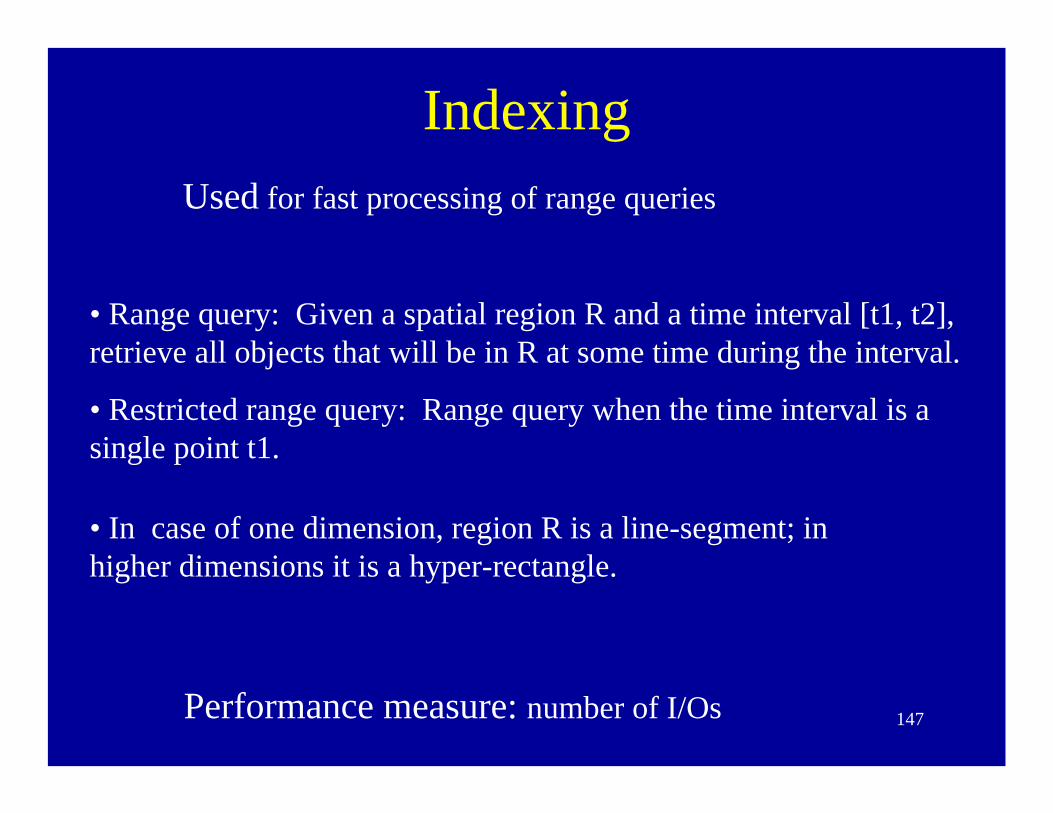
IndexingUsed for fast processing of range queries
• Range query: Given a spatial region R and a time interval [t1, t2], retrieve all objects that will be in R at some time during the interval.
• Restricted range query: Range query when the time interval is a single point t1.
• In case of one dimension, region R is a line-segment; in higher dimensions it is a hyper-rectangle.
Performance measure: number of I/Os

148
Indexing Methods•Primal Space Method:
• Consider the space together with time as an additional axis. Object movements form straight lines in this space (when moving with constant velocity).
•Consider the hyper rectangle X formed by the region R of the query and the given time interval. The answer is the set of objects whose lines intersect X.

149
Primal Space
Time T
Posi
tion
X
Query Q1: region R is the x-interval [1,2], time interval is the single point 1.
Q2: R is the x-interval [1,3], time interval is [2,3]
o3
o2
x2x1
o1
150
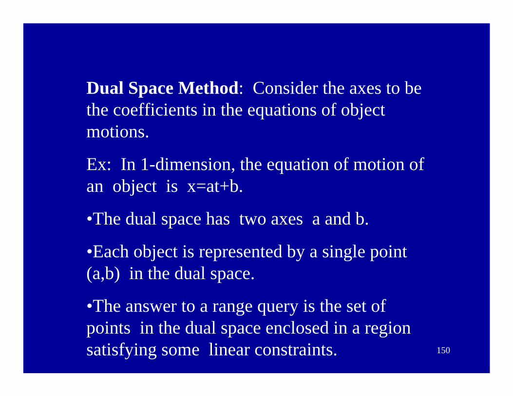
Dual Space Method: Consider the axes to be the coefficients in the equations of object motions.
Ex: In 1-dimension, the equation of motion of an object is x=at+b.
•The dual space has two axes a and b.
•Each object is represented by a single point (a,b) in the dual space.
•The answer to a range query is the set of points in the dual space enclosed in a region satisfying some linear constraints.

151
Answer to query Q1: all the points in the strip.
Dual Space
0
1
2
3
0 1 2 3a->
b->
o1
o2
o3

152
Q: Retrieve objects for which dynamic attribute has value v a≤v≤b at time t.
Spatial indexing to find objects that satisfy ( intersect ) query.
.o1
.o2
.o3 slopequery
intercept
dual
dynamic attribute value
o2o1
o3
timet
ba Q primal
153
Primal Space Methods
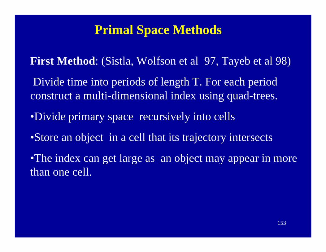
First Method: (Sistla, Wolfson et al 97, Tayeb et al 98)
Divide time into periods of length T. For each period construct a multi-dimensional index using quad-trees.
•Divide primary space recursively into cells
•Store an object in a cell that its trajectory intersects
•The index can get large as an object may appear in more than one cell.
154
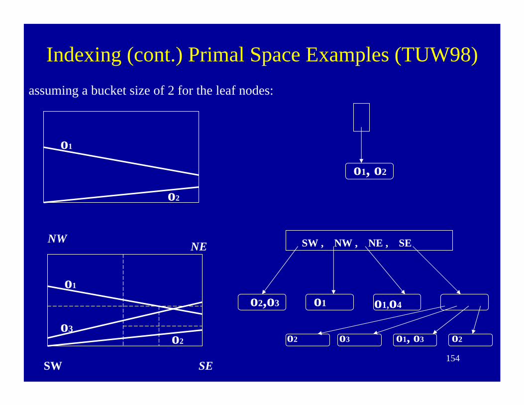
Indexing (cont.) Primal Space Examples (TUW98)assuming a bucket size of 2 for the leaf nodes:
o1
o2
o1, o2
SW , NW , NE , SENWNE
SESW
o2,o3 o1
o2
o1
o3
o1,o4
o2 o3 o1, o3 o2

155
Performance analysis of primal plane representation using quadtrees. Tayeb, Ulusoy, Wolfson; Computer Journal, 1998
Example of implication:30,000 objects 3 I/O’s per range query

156
Primal Space Methods--- Contd
Second Method: (kinetic data structure) only for one dimensional motion.
•At any point in time we can linearly order objects based on their location. The ordering changes at those times when object trajectories cross.
•Fix a time period T and determine the orderings at the beginning and at T.
•Find the crossing points t1,t2,…,tm of the objects.

157
o1
o2
o3
Time T
Spac
e X
Determine ordering between crossing points
t1 t2 t3

158
•Obtain the orderings between the crossings. Build binary search trees T1,…,Tm based on them.
•To retrieve objects in the space interval I at time t do as follows:
•Find a value j such that time t falls in the jth time interval.
•Use the search tree Tj to find all objects in the space interval I at that time.
Has space complexity O(n+m) and time complexity O(log (n+m)) where m is the number of crossings and n = N/B; N is the number of moving point objects, and B is the block size.

159
Primal Space Methods (continued)• Third method: Saltenis et. al. 2000
• Time parameterized R*-trees (TPR)
• works for motion in any number of dimensions.
• Similar to R*-trees except that the MBRs are time parameterized.
• Objects are clustered and grouped into MBRs.
• MBRs are enclosed into bigger MBRs.
• They are arranged into a R*-tree.
• Each MBR has the following information.
• Its coordinates
• the min and max velocities of objects (in each direction).

160
o1 o2
X
Y
Leaf level MBRs overtime
o3
o4
o1
o2
X
Y
o3
o4
At Time t At Time t+2
161
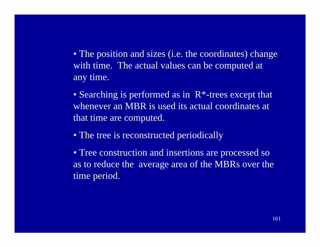
• The position and sizes (i.e. the coordinates) change with time. The actual values can be computed at any time.
• Searching is performed as in R*-trees except that whenever an MBR is used its actual coordinates at that time are computed.
• The tree is reconstructed periodically
• Tree construction and insertions are processed so as to reduce the average area of the MBRs over the time period.

162
Dual Space Methods
• similar to quad trees except:
• Employs Partition trees (used in computational geometry)
• Partition trees use simplicial partitions of sets of points.
• A simplicial partition of S is a set of pairs (S1,D1),…,(Sr,Dr) such that S1, …Sr is a partition of S. Di is a triangle enclosing points in Si.
[Kollios et al 99 (1-dimension), Agarwal et al 00 (2-dimensions)]

163
For the given set of moving point objects, a partition tree is constructed satisfying the following properties.
• The leaves are blocks containing moving objects.
• A triangle is associated with each node in the tree.
•The vertices of the triangle are stored in the node.
•This triangle contains all the object points of the sub-tree.
• The sets of points and triangles associated with the children of a node form a balanced simplicial partition of the set of nodes of the parent.
• The size of the tree is O(n) and the height O(log n).
164
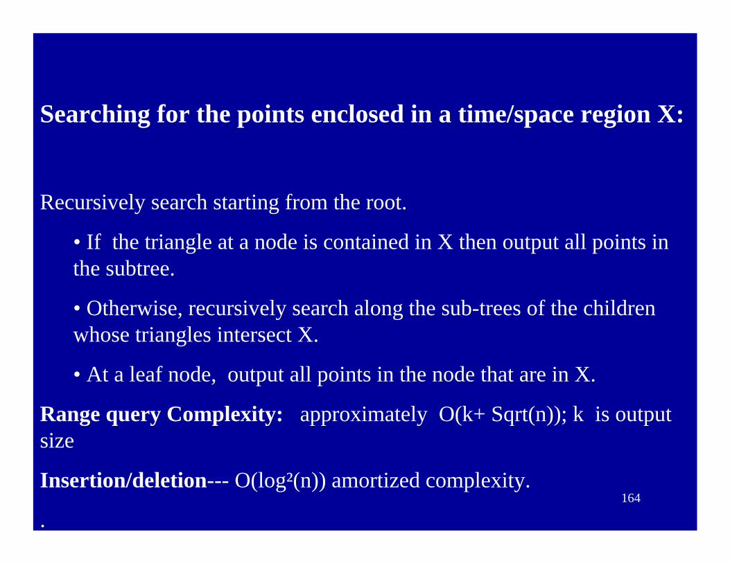
Searching for the points enclosed in a time/space region X:
Recursively search starting from the root.
• If the triangle at a node is contained in X then output all points in the subtree.
• Otherwise, recursively search along the sub-trees of the children whose triangles intersect X.
• At a leaf node, output all points in the node that are in X.
Range query Complexity: approximately O(k+ Sqrt(n)); k is output size
Insertion/deletion--- O(log²(n)) amortized complexity.
.

165
Solution Paradigm
• Geometric Problem Representation in Multidimensional Time-Space
• Spatial Indexing of Geometric Representation

166
Indexing with Uncertaintyo1
o2
o3
possibly
time
dynamic attribute value
intercept
slopequery
o1o2
o3 possibly
definitely
definitely
167
Indexing References[1] Yannis Theodoridis, Timos K. Sellis, Apostolos Papadopoulos and Yannis Manolopoulos, Specifications for Efficient Indexing in Spatiotemporal Databases, In the proceedings of Statistical and Scientific Database Management, p123-132, 1998[2] Jamel Tayeb, Our Ulusoy and Ouri Wolfson, A Quadtree-Based Dynamic Attribute Indexing Method, in The Computer Journal, volume 41, no.3, p185--200, 1998 [3] D. Pfoser, Y. Theodoridis and C. Jensen, Indexing Trajectories of Moving Point Objects, Dept. of Computer Science, University of Aalborg, 1999.[4] M. Kornacker, High - Performance Extensible Indexing, VLDB 1999.[5] S. Saltenis and C. S. Jensen and S. T. Leutenegger and M. A. Lopez, Indexing the positions of continuously moving objects, Time Center, 1999[6] D. Kollios and D. Gunopulos and V. J. Tsotras, On indexing mobile objects, ACM PODS 1999.[7] W. Chen and J. Chow and Y. Fuh and J. grandbois and M. Jou and N. Mattos and B. Tran and Y. Wang, High level indexing of User -- Defined types, VLDB 1999.[8] M.A. Nascimento and J.R.O. Silva and Y. Theodoridis, Evaluation of Access Structures for Discretely Moving Points, in the proceedings of Spatio-Temporal Database Management, 1999.[9] A. K. Agarwal and L. Arge and J. Erickson, Indexing Moving Points, ACM PODS 2000. [10] D. Pfoser and C. S. Jensen and Y. Theodoridis, Novel Approaches to the Indexing of Moving Object Trajectories, VLDB 2000.[11] Simonas Saltenis and Christian S. Jensen and Scott T. Leutenegger and Mario A. Lopez, Indexing the Positions of Continuously Moving Objects. SIGMOD 2000.[12] S. Saltenis and C. S. Jensen and S. T. Leutenegger and M. A. Lopez, Indexing the Moving Objects for Location-based Services, Time Center, 2001[13] Zhexuan Song and Nick Roussopoulos, Hashing Moving Objects, in the proceedings of Mobile Data Management, p161-172, 2001.

168
[14] Susanne Hambrusch and Chuan-Ming Liu and Walid G. Aref and Sunil Prabhakar, Query Processing in Broadcasted Spatial Index Trees, in the proceedings of Spatial and Temporal Databases, July 2001, Los Angeles, CA.[15] Marios Hadjieleftheriou and George Kollios and Vassilis J. Tsotras and Dimitrios Gunopulos, Efficient Indexing of Spatiotemporal Objects, in the proceedings of Extending Database Technology, p251-268, 2001[16] Yufei Tao and Dimitris Papadias, MV3R-Tree: A Spatio-Temporal Access Method for Timestamp and Interval Queries. VLDB 2001.[17] Hae Don Chon, Divyakant Agrawal, Amr El Abbadi, Using Space-Time Grid for Efficient Management of Moving Objects, MobiDE 2001[18] Hae Don Chon, Divyakant Agrawal, Amr El Abbadi, Storage and Retrieval of Moving Objects, Mobile Data Management (MDM) 2001. [19] Sunil Prabhakar and Y. Xia and D. Kalashnikov and W. Aref and S. E. Hambrusch, Query Indexing and Velocity Constrained Indexing: Scalable Techniques for Continuous Queries on Moving Objects, IEEE Transactions on Computers, Special Issue on DBMS and Mobile Computing, 2002[20] Dongseop Kwon and Sangjun Lee and Sukho Lee, Indexing the Current Positions of Moving Objects Using the Lazy Update R-tree, in the proceedings of MDM2002, 2002.[21] Ravi Kanth V Kothuri, Siva Ravada and Daniel Abugov, Quadtree and R-tree Indexes in Oracle Spatial: A Comparison using GIS Data, In Proceedings of SIGMOD 2002.[22] Special Issue on Indexing of Moving Objects. Bulletin of the Technical Committee on Data Engineering, June 2002, Vol.25 No.2. [23] Mahdi Abdelguerfi, Julie Givaudan, Kevin Shaw, Roy Ladner, The 2-3TR-tree, a trajectory-oriented index structure for fully evolving valid-time spatio-temporal datasets, Proceedings of the 10th ACM international symposium on Advances in geographic information systems, 2002.

169
[24] Simonas Šaltenis, Christian S. Jensen, Indexing of Moving Objects for Location-Based Services, in proc. of the 18th international conference on Data Engineering (ICDE'02).[25] Yufei Tao and Dimitris Papadias, Adaptive Index Structures, In proc, of the 28th international conference on very large databases, VLDB 2002.[26] Hae Don Chon, Divyakant Agrawal, Amr El Abbadi, Data Management for Moving Objects, Data Engineering Bulletin. June 2002. [27] Hae Don Chon, Divyakant Agrawal, Amr El Abbadi, Query Processing for Moving Objects with Space-Time Grid Storage Model, Mobile Data Management (MDM) 2002. [28] Rui Ding, Xiaofeng Meng, Yun Bai, Efficient Index Update for Moving Objects with Future Trajectories, Proceedings of the 8th international conference on Database Systems for Advanced Applications (DASFAA), 2003.[29] Yuni Xia, Sunil Prabhakar, Q+Rtree: Efficient Indexing for Moving Object Databases, Proceedings of the 8th international conference on Database Systems for Advanced Applications (DASFAA), 2003.[30] Dimitris Papadias, Yufei Tao, Jimeng Sun, The TPR*-Tree: An Optimized Spatio-Temporal Access Method for Predictive Queries, In proc, of the 29th international conference on very large databases, VLDB 2003.[31] Mong Li Lee, Wynne Hsu, Christian S. Jensen, and Keng Lik Teo, Supporting Frequent Updates in R-Trees: A Bottom-Up Approach, In proc, of the 29th international conference on very large databases, VLDB 2003.

170
Outline• Background
– Location technologies, applications
– demo
• Research issues
– Location modeling/management
– Linguistic issues
– Uncertainty/Imprecision
– Indexing
– Synthetic datasets
– Compression/data-reduction
– Joins and data mining
171
Contents• Motivation: Collecting huge real spatio-temporal
data is difficult.
• Idea: random generation of data
• Methods
• Generate_Spatio_Temporal_Data(GSTD) [1, 2]• Brinkhoff's Approach [3, 4]• Saglio and Moreira's Generator [5]• CitySimulator [6, 7]• Generation of Pseudo Trajectories [8]

172
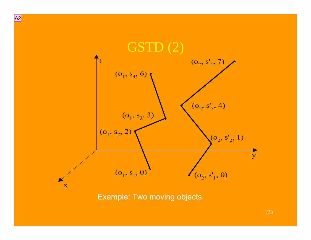
GSTD (1)• Model
– Bounded 2D free space.– objects:
• Point objects: vehicles, pedestrians• Region objects: weather phenomena
– purpose: evaluation of indexing methods• Basic operations
– define a set of objects with starting position for each– compute new timestamp– compute new spacestamp– compute new spacestamp’s extension
A1

Slide 172
A1 Three random & probability distribution uniform; Skew; Gaussian.Administrator, 12/31/2002
173
GSTD (2)
Example: Two moving objects
A2

Slide 173
A2 This example is only for point objects
If an object leaves the spatial data space, different approaches can be applied: the position remains unchanged; the position is adjusted to fi into the data space; the oject re-enters the data space at the opposite edge of the data space.Administrator, 1/2/2003

174
Brinkhoff's Approach• Model
– 2D– based on a network (TIGER files)– objects:
• point objects • region objects (weather)
– purpose: evaluation of indexing• Basic operations
– generate objects every time unit• generate starting points• generate length of route (depending on object
class)• generate destination for each object• compute the route• compute the trajectory by generating a random
speed every time unit (based on capacity, weather, edge class, etc.)
x
y
t
(o1, s1, 0)
(o1, s2, 2)
(o1, s3, 3)
(o1, s4, 6)
(o2, s'1, 0)
(o2, s'2, 2)
(o2, s'3, 3)
(o2, s'4, 6)
Example: Two moving objects:
o1: A car; o2: A truck
A3

Slide 174
A3 The network can be 1. synthetic network 2. real network: TIGER/Line files; SEQUOIA 2000 Storage benchmark.
The destination is computed by the starting point & the length of route.
Three methods for computing the starting points: data-space oriented approach (DSO); region-based approach (RB); network-based approach (NB).
A* algorithm for computing the route.Administrator, 12/31/2002

175
Saglio and Moreira's Generator•Model– 2D frame– Motivating scenario: modeling the motion of fishing boats– objects:
• Harbors: static• Fishing ships: moving objects• Good spots & bad spots: center fixed, dynamic shape• Shoals: dynamic center & shape
– purpose: evaluation of indexing methods
•Basic operations– define objects– define changes for each object
– criterion for motion: proximity (e.g. shoals to good spots)
A4

Slide 175
A4 spots (bad&good): appear at random locations & times & extension first expansion, then shrinkingshoals of fish: random center, velocity & extension seek for a good spot (the nearest one)harbors: on the boundary of the framefishing ships: goes after a selected shoal (a good spot) & avoid storms(bad spots) criterion for selection: proximityAdministrator, 12/31/2002
176
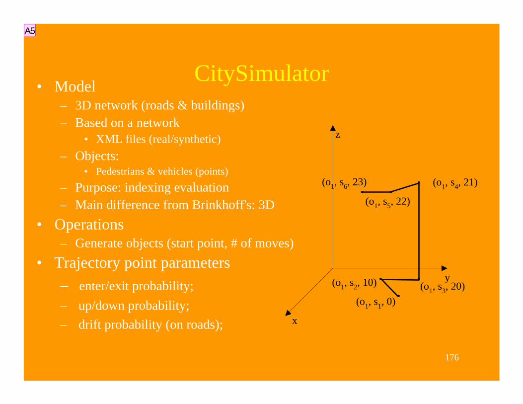
CitySimulator• Model
– 3D network (roads & buildings)– Based on a network
• XML files (real/synthetic)– Objects:
• Pedestrians & vehicles (points)– Purpose: indexing evaluation– Main difference from Brinkhoff's: 3D
• Operations– Generate objects (start point, # of moves)
• Trajectory point parameters– enter/exit probability;– up/down probability;– drift probability (on roads); x
z
(o1, s1, 0)
(o1, s2, 10)
(o1, s4, 21)
(o1, s5, 22)
y
(o1, s6, 23)
(o1, s3, 20)
A5

Slide 176
A5 For the object o1, locations s1, s2 & s3 are on the same plane z = 0; locations s4, s5 & s6 are on the same plane z = 18.
This example simulates one person drives a car to his office building, and go to his office which locates on the 18th floor (z = 18) (firstby the elevator and then by walking).
Parameters: enter/exit probability; up/down probability; drift probability (on roads); scatter probability (on intersections); traffic model.Administrator, 1/3/2003

177
Pseudo trajectories [8]
• Realistic synthetic trajectories by superimposing real speed variations on random routes

178
Real Trajectories Dataset
• Real Trajectories– Define Drive trip– Repeatedly read the (longitude, latitude, time)
from a Differential GPS device connected to a laptop
– Every two seconds
179
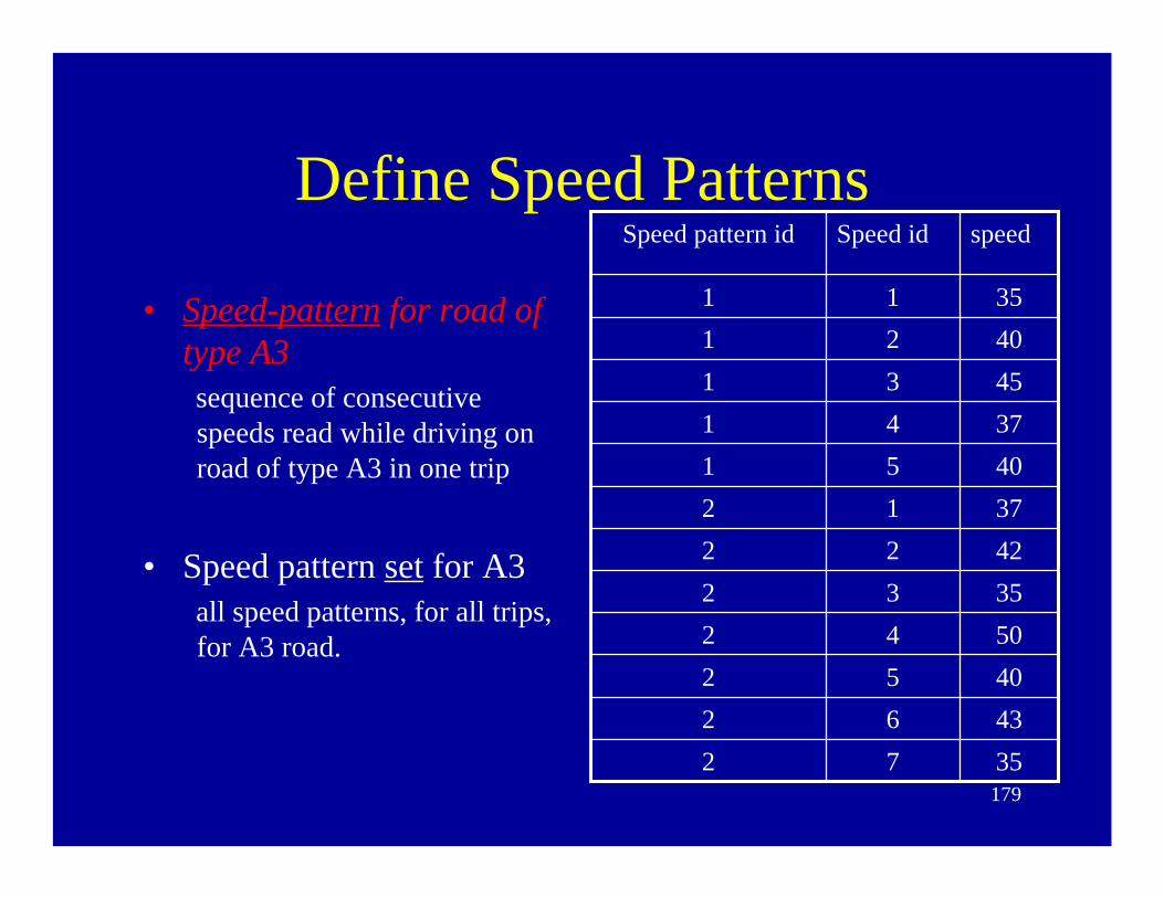
Define Speed Patterns
• Speed-pattern for road of type A3sequence of consecutive speeds read while driving on road of type A3 in one trip
• Speed pattern set for A3all speed patterns, for all trips, for A3 road.
37414051371242223532504240524362
3511
3572
45314021
speedSpeed idSpeed pattern id

180
The route
Pseudo Trajectory Generation
1. Generate random route and set v=0
2. Pick a random speed pattern R for the current street type that has speed v.
3. Continue R to the end of the pattern or end of road, whichever comes first.
4. Set v to last speed and go to 2.
A13

Slide 180
A13 a, b, c are speeds that equal to current speed v = 35 mph. Randomly select speed pattern 1, starting from a to compute the new position and timestamp on the first A1 street.Administrator, 12/31/2002

181
References[1] Theodoridis Y., Silva J.R.O., Nascimento M.A., "On the Generation of Spatiotemporal Datasets". In Proceedings of the 6th International Symposium on large Spatial Databases (SSD), Hong Kong, China, July 20-23, 1999. LNCS 1651, Springer, pp. 147-164.[2] Pfoser D., Theodoridis Y., "Generating Semantics-Based Trajectories of Moving Objects". Intern. Workshop on Emerging Technologies for Geo-Based Applications, Ascona, 2000.[3] Brinkhoff Thomas, "Generating Network-Based Moving Objects". In Proceedings of the 12th International Conference on Scientific and Statistical Database Management, Berlin, Germany, July 26-28, 2000.[4] Brinkhoff Thomas, "A Framework for Generating Network-Based Moving Objects". Technical Report of the IAPG, http://www2.fh-wilhelmshaven.de/oow/institute/ iapg/personen/brinkhoff/paper/TBGenerator.pdf[5] Jean-Marc Saglio, José Moreira, "Oporto: A Realistic Scenario Generator for Moving Objects". In Proceedings of the 10th International Workshop on Database and Expert Systems Applications, IEEE Computer Society, Florence, Italy, September 1-3, August 30-31, 1999, pp. 426-432, ISBN 0-7695-0281-4. [6] CitySimulator: http://alphaworks.ibm.com/tech/citysimulator[7] Jussi Myllymaki and James Kaufman, "LOCUS: A Testbed for Dynamic Spatial Indexing". In
IEEE Data Engineering Bulletin 25(2), p48-55, 2002.[8] Huabei Yin and Ouri Wolfson, “Accuracy and Resource Consumption in Tracking Moving Objects ”, Symposium on Spatio-temporal Databases, Santorini Island, Greece, 2003.

182
Outline• Background
– Location technologies, applications
– demo
• Research issues
– Location modeling/management
– Linguistic issues
– Uncertainty/Imprecision
– Indexing
– Synthetic datasets
– Compression/data-reduction
– Joins and data mining
183
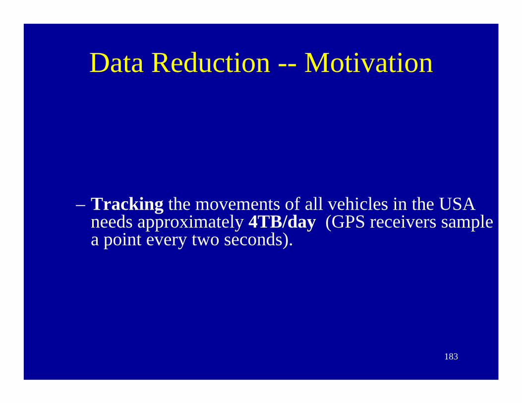
Data Reduction -- Motivation
– Tracking the movements of all vehicles in the USA needs approximately 4TB/day (GPS receivers sample a point every two seconds).

184
Trajectory Reduction
• Line simplification: approximate a trajectory by another which is not farther than ε.
ε
ε

185
Distance Functions• The distance functions considered
are:– E3: 3D Euclidean distance.
– E2: Euclidean distance on 2D projection of a trajectory
– Eu: the Euclidean distance of two trajectory points with same time.
– Et: It is the time distance of two trajectory points with same location or closest Euclidean distance.
• #(T'2) ≤ #(T'3) ≤ #(T'u), which is also verified by experimental saving comparison.

186
Soundness of Distance Functions • Soundness: bound on the error when answering spatio-temporal
queries on simplified trajectories.
• The appropriate distance function depends on the type of queriesexpected on the database of simplified trajectories.– If all spatio-temporal queries are expected, then Eu And Et should be
used. – If only where_at, intersect, and nearest_neighbor queries are expected,
then the Eu distance should be used.
Sound when (a) the distance function
D of join is metric (b) E is weaker than D.
Spatial Join
NoNoYesNoEt
YesYesNoYesEu
NoNoNoNoE3
NoNoNoNoE2
Nearest_Neighbor
IntersectWhen_atWhere_at

187
Savings (of past trajectories):
• ε=0.1 ==> reduction to at most 1% for most distances.• Better than the Wavelet compression.
The Optimal Simplification DP Simplification

188
Aging of Trajectories
• Increase ε as time progresses
T’ =Simp(Simp(T, ε1 )) = Simp(T, ε2) , ε1≤ε2
• Valid for all distance functions when using the DP simplification algorithm.

189
Outline• Background
– Location technologies, applications
– demo
• Research issues
– Location modeling/management
– Linguistic issues
– Uncertainty/Imprecision
– Indexing
– Synthetic datasets
– Compression/data-reduction
– Joins and data mining
190
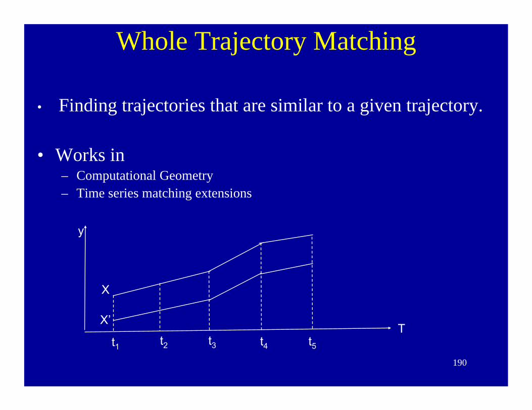
• Finding trajectories that are similar to a given trajectory.
• Works in – Computational Geometry– Time series matching extensions
Whole Trajectory Matching
t1 t2 t3 t4 t5T
y
X
X’

191
Maximum Euclidean Distance
D(X,X’) = MAX t1≤t≤t2 [d(X(t), X’(t))]
XX’
D(X,X’)
t1 t2
X
Ttmax

192
Root Mean Error Euclidean Distance
D(X,X’) = (1/5*(d12 + d2
2+ d32+ d4
2+ d52))1/2
Example: Measuring the error of an estimated trajectory.
X
X’d1 d2
d3 d4d5
y
Tt1 t2 t3 t4 t5

193
Minimum Euclidean Distance
D(X,X’) = MIN t1≤t≤t2 [d(X(t), X’(t))]
Example: collision detection.
XX’
D(X,X’)
t1 t2
X
Ttmin

194
Geometric Transformation --- Translation
• A geometric transformation consisting of a constant offset• every point (x, y, t) becomes (x+ε, y +δ, t + π) after a
translation.
Example: 2 home-office trajectories (on different days) are similar after time-translation

195
Geometric Transformation --- Rotation• Turns a trajectory by an angle about a fixed point. • The rotation is limited in the X-Y sub-space.
Translation, rotation are rigid transformations.Ex: similar motion patterns in different cities/times
196
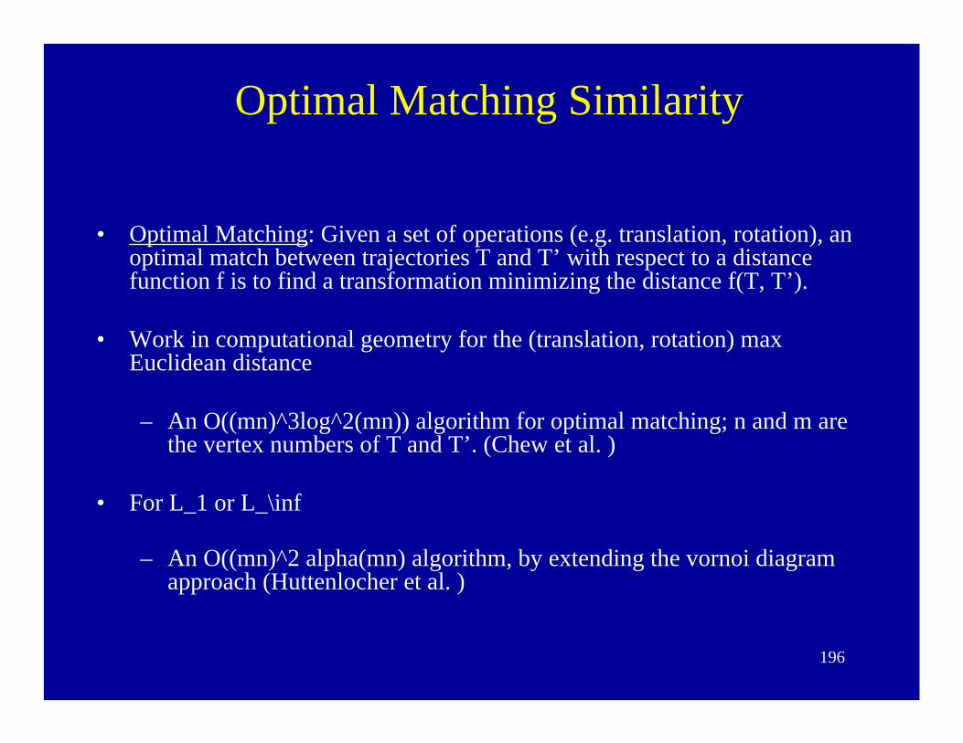
Optimal Matching Similarity
• Optimal Matching: Given a set of operations (e.g. translation, rotation), an optimal match between trajectories T and T’ with respect to a distance function f is to find a transformation minimizing the distance f(T, T’).
• Work in computational geometry for the (translation, rotation) max Euclidean distance
– An O((mn)^3log^2(mn)) algorithm for optimal matching; n and m are the vertex numbers of T and T’. (Chew et al. )
• For L_1 or L_\inf
– An O((mn)^2 alpha(mn) algorithm, by extending the vornoi diagram approach (Huttenlocher et al. )

197
Longest Common Subtrajectory Similarity
• Trajectories maybe similar in pattern but of different length.• Longest Common Subtrajectory Similarity(LCSS) uses the length of
continuous similar subtrajectories to evaluate the similarity:
),min()',(
'TT LengthLengthTTLNSS

198
Time Scaling
199
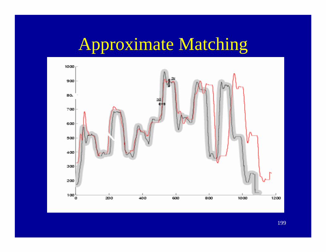
Approximate Matching
200
Finding the Longest Common Subtrajectory
• M. Vlachos et al. give a dynamic programming algorithm using – translation, – approximate matching, and – time scalingto compute the LCSS.
• The time complexity of their algorithm is O(n+m)3δ3),where m and n are the numbers of vertices, δ is the maximal allowed time difference between two compared points

201
References
[1] M. Vlachos, G. Kollios & D. Gunopulos. Discovering Similar Multidimentional Trajectories. In ICDE, San Jose, CA, 2002.
[2] S.-L. Lee, S.-J. Chun, D.-H. Kim, J.-H. Lee & C. Chung. Similarity Search for Multidimensional Data Sequences. In ICDE, San Diego, USA, 2000.
[3] T. Kahveci, A.K. Singh & A. Guerel. Similarity Searching for Multi-attribute Sequences. In SSDBM, 2002, Edinburgh, Scotland.
[4] T. Kahveci, A. K. Singh, and A. Guerel. Shift and scale invariant search of multi-attribute time sequences. Technical report, UCSB, 2001.
[5] Y. Yanagisawa, J. Akahani & T. Satoh. Shape-based Similarity Query for Trajectory Data, 2002.

202
[6] H.V. Jagadish. Linear Clustering of Objects with Multiple Attributes. Proceedings of ACM SIGMOD Int’l Conference on Management of Data, pages 332-342, Atlantic City, New Jersey, May 1990.
[7] H. Alt, L. J. Guibas. Discrete Geometric Shapes: Matching, Interpolation, and Approximation A survey.
[8]E. Keogh & S. Kasetty. On the Need for Time Series Data Mining Benchmarks: A Survey and Empirical Demonstration. In SIGKDD ’02, July, 23-26 2002, Edmonton, Alberta, Canada, 2002.
[9]M. L. Hetland. A Survey of Recent Methods for Efficient Retrieval of Similar Time Sequences. To appear in Data Mining in Time Series Databases. World Scientific, 2003.
[10] R. Agrawal, C. Faloutsos and A. Swami. Efficient Similarity Search In Sequence Databases. In Proc. Of the Fourth International Conference on foundations of Data Organization and Algorithms, Chicago, October 1993. Also in Lecture Notes in Computer Science 730, Springer Verlag, pp69-84, 1993.

203
[11] C. Faloutsos, M. Ranganathan, and Y. Manolopoulos. Fast subsequence matching in time-series databases. In Proc. Of the ACM SIGMOD Conference on Management of Data, Minneapolis MN, May 1994.
[12] R. Agrawal, K.I. Lin, H. S. Sawhney and K. Shim (1995). Fast Similarity Search in the Presence of Noise, Scaling, and Translation in Time-Series Databases. In Proceedings of the 21st Int’l Conference onVLDB Conference, Zurich,Switzerland, Sept, 1995.
[13] L. P. Chew, M. T. Goodrich, D. P. Huttenlocher, K. Kedem, J. M. Kleinberg, and D. Kravets, Geometric pattern matching under Euclidean Motion, In Proc 5th Canada Conference of ComputionalGeometry. pp151-156 Waterloo, Canada 1993.
[14] D. P. Huttenlocher, K. Kedem, and M. Sharir, The upper envelope of Voronoi surfaces and its applications. Discrete Comput Geom. 9:267-291, 1993.

204
Location Awareness in Querying Mobile Environments
• An application of distributed/mobile/incomplete location database
• Each node stores its location, location of its neighbors, possibly location of destination of query

205
Example Applications
What are the traffic conditions 2 miles ahead of me?
Where are the available parking slots around my location?
206
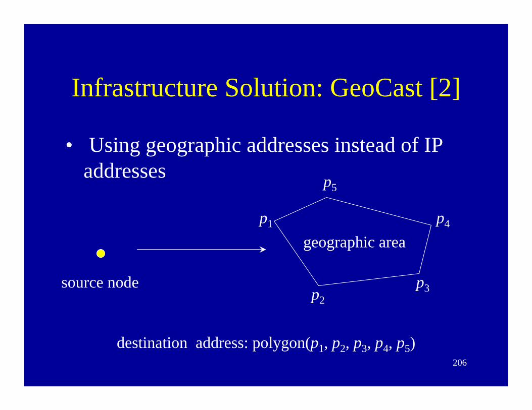
Infrastructure Solution: GeoCast [2]
• Using geographic addresses instead of IP addresses
source node
geographic area
destination address: polygon(p1, p2, p3, p4, p5)
p1
p2p3
p4
p5

207
How GeoCast Works
(A) R1
R2 (convex hull of A, B, C)
R3 (convex hull of B, C)
Moving object. Each equipped with a GPS
Mobile Support Station Router
H1N1
N2 N3
A B C

208
Infrastructureless Solution: Mobile Ad-hoc Networks
• MANET: A set of moving objects communicating without the assistance of base stations
• A MANET uses peer-to-peer multi-hop routing to provide source to destination connectivity
• Need to do better than flooding (in b/w, power)• See [9] for a survey of routing in ad-hoc networks

209
Location Based Routing
• The destination area or the location of the destination node is known by the source and used for message delivery.
• An intermediate node discovers neighbors and their locations and moving directions.
210
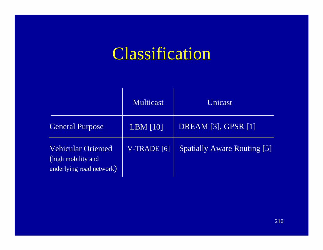
Classification
Vehicular Oriented(high mobility and underlying road network)
General Purpose
Multicast Unicast
LBM [10] DREAM [3], GPSR [1]
V-TRADE [6] Spatially Aware Routing [5]

211
Location Based Multicast (LBM)
destination area
forwarding zone of SS
J
I
KL
forwarding zone of L
Each node floods to all the nodes within a forwarding zone. Each node is aware of its location and forwarding zone.
212
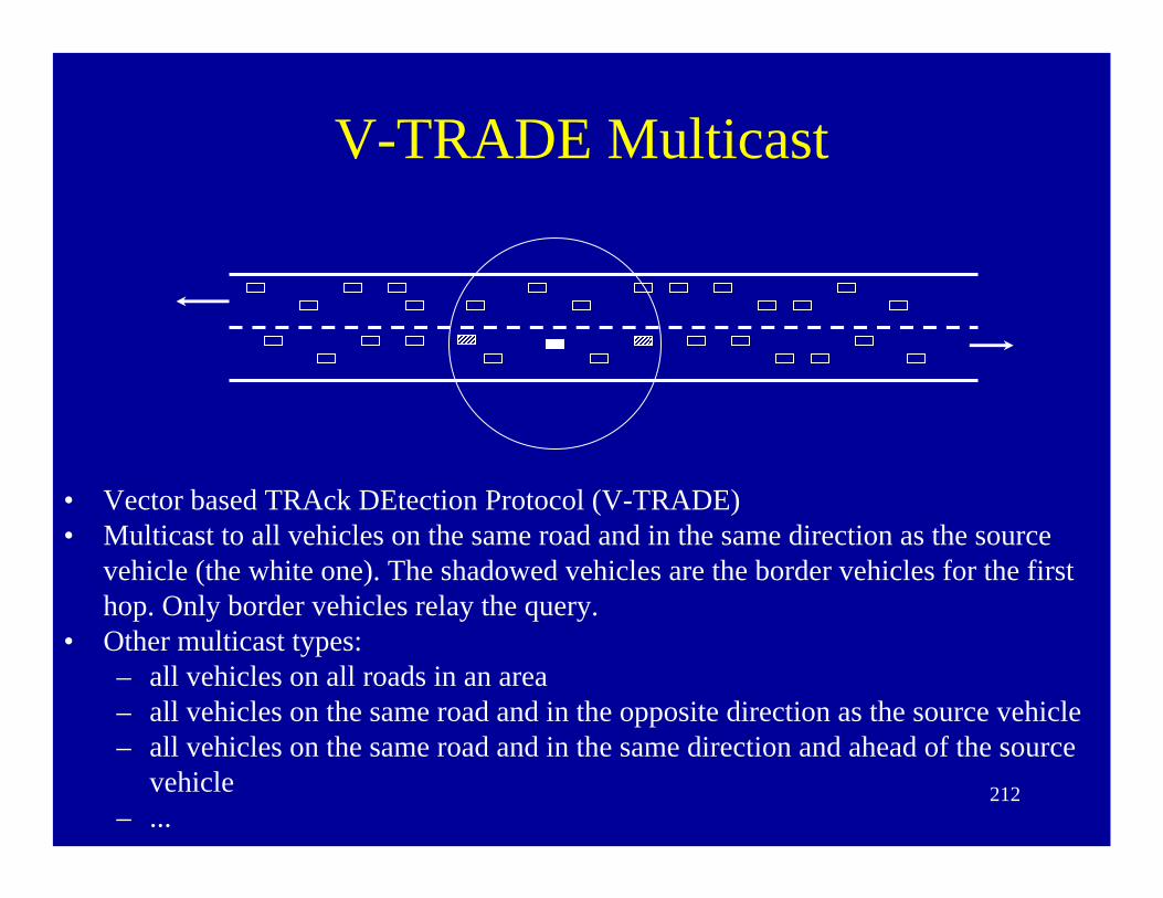
V-TRADE Multicast
• Vector based TRAck DEtection Protocol (V-TRADE)• Multicast to all vehicles on the same road and in the same direction as the source
vehicle (the white one). The shadowed vehicles are the border vehicles for the first hop. Only border vehicles relay the query.
• Other multicast types: – all vehicles on all roads in an area– all vehicles on the same road and in the opposite direction as the source vehicle– all vehicles on the same road and in the same direction and ahead of the source
vehicle– ...

213
Greedy Geographic Unicast
When there is no neighbor closer to the destination than x:select a farther neighbor, according to planar graph face traversal rule.

214
Distance Routing Effect Algorithm for Mobility (DREAM)
• S sends a message to D at time t. • Always floods to all the objects within the wedges.
S
I
J
The area D can possibly be in at tas far as S knows.
The area D can possibly be in at tas far as I knows.
The latest location update of Dreceived by S.
The latest location update of Dreceived by I.

215
Spatial Constraint of Vehicular Networks
The road network determines proximity.

216
How to map from the ID of a node to its location ?

217
Location Service in DREAM
α
α d
• Each node periodically floods its locations.• The location message in the 2i-th period travels twice as far as the one in the i-th period. (radius indicated in the message)

218
Grid Location Service
• Fixed hierarchical partition• Location servers of 17 is the least ID higher than 17 in each partition

219
References1. B. Karp and H. T. Kung. GPSR: Greedy perimeter stateless routing for wireless networks. In Proc. Of
ACM/IEEE MOBICOM, Boston, MA, Aug. 2000.2. J. C. Navas and T. Imielinski. GeoCast – Geographic Addressing and Routing. In Proc. of ACM/IEEE
MOBICOM, Budapest, Hungary, Sept. 1997.3. S. Basagni, I. Chlamtac, V. R. Syrotiuk and B. A. Woodward. A Distance Routing Effect Algorithm
for Mobility (DREADM). In Proc. of ACM/IEEE MOBICOM, 1998.4. J. Li, J. Jannotti, D. De Couto, D. Karger and R. Morris. A Scalable Location Service for Geographic
Ad Hoc Routing. In Proc. of ACM/IEEE MOBICOM, Boston, MA, 2000, pp. 120-130.5. J. Tian, L. Han, K. Rothermel, and C. Cseh. Spatially Aware Packet Routing for Mobile Ad Hoc Inter-
Vehicle Radio Networks. To appear in the IEEE 6th International Conference on Intelligent Transportation Systems (ITSC), Shanghai, China, October 12-15, 2003.
6. M. Sun, W. Feng, T. Lai, et al. GPS-Based Message Broadcasting for Inter-vehicle Communication. In Proc. of the 2000 International Conference on Parallel Processing, Toronto, Canada, Aug. 2000, p. 279.
7. Q. Li and D. Rus. Sending Messages to Mobile Users in Disconnected Ad-hoc Wireless Networks. In Proc. 6th Annual ACM/IEEE International Conference on Mobile Computing, MOBICOM'00, 2000.
8. Vahdat and D. Becker. Epidemic Routing for Partially Connected Ad Hoc Networks, Technical Report CS-200006, Duke University, April 2000. http://citeseer.nj.nec.com/vahdat00epidemic.html
9. E. Royer and C. Toh, A Review of Current Routing Protocols for Ad Hoc Mobile Wireless Networks, IEEE Personal Communications, pages 46--55, Apr. 1999.
10. Y. Ko and N. Vaidya. Geocasting in Mobile Ad Hoc Networks: Location Based Multicast Algorithms.In Proc. of the Second IEEE Workshop on Mobile Computer Systems and Applications, New Orleans, Louisiana, Feb. 1999.

220
Conclusion• Background
– Location technologies, applications
– demo
• Research issues
– Location modeling/management
– Linguistic issues
– Uncertainty/Imprecision
– Indexing
– Synthetic datasets
– Compression/data-reduction
– Joins and data mining

221
New Research Topics• Distributed/Mobile query and trigger processing
with incomplete/imprecise location information• Extensible and visual languages• Comparison of indexing methods
• Uncertainty for moving objects that do not report their location
• Data Mining

222
New Research Topics (Continued)
• Privacy/Security
• Location prediction
• Performance/indexing for join queries
Related Documents