Bayesian propagation for perceiving moving objects

March 31, 2006 17:10 WSPC/INSTRUCTION FILE Boccignone-IJPRAI

International Journal of Pattern Recognition and Artificial Intelligencec© World Scientific Publishing Company

BAYESIAN PROPAGATION FOR PERCEIVING

MOVING OBJECTS

GIUSEPPE BOCCIGNONE, ANGELO MARCELLI and PAOLO NAPOLETANO

Dipartimento di Ingegneria dell’Informazione e Ingegneria ElettricaUniversita di Salerno

via Ponte Melillo 1, 84084 Fisciano (SA), Italyboccig,amarcelli,[email protected]

VITTORIO CAGGIANO

Dipartimento di Informatica e SistemisticaUniversita di Napoli Federeico II via Claudio 21, 80125 Napoli, Italy

[email protected]

GIANLUCA DI FIORE

CoRiTeLvia Ponte Melillo 1, 84084 Fisciano (SA), Italy

[email protected]

In this paper we address the issue of how form and motion can be integrated in orderto provide suitable information to attentively track multiple moving objects. Such in-tegration is designed in a Bayesian framework, and a Belief Propagation technique isexploited to perform coherent form/motion labelling of regions of the observed scene.Experiments on both synthetic and real data are presented and discussed.

Keywords: Bayesian Belief Propagation, motion estimation and segmentation, visualattention, tracking.

1. Introduction

Visual attention not only restricts various types of visual processing to certain spa-

tial areas of the visual field8, but also accounts for object-based information, so that

attentional limitations are characterized in terms of the number of discrete objects

which can be simultaneously processed15. Several theories have been concerned with

how object-based individuation, tracking and access is realized and, in particular,

Pylyshyn’s FINST (FINgers of INSTantiation) proposal has complemented such

theories15. The model is based on a finite number, say k ≃ 4, 5, of visual indexes

(fingers, inner pointers) that can be assigned to various items and serve as means

of access to such items for higher level processes that allocate focal attention. The

visual indexes bestow a processing priority, insofar as they allow focal attention to

be shifted to indexed items, possibly moving, either under volitional control or due

to habituation factors, without first searching for them by spatial scanning.

1

March 31, 2006 17:10 WSPC/INSTRUCTION FILE Boccignone-IJPRAI

2 G. Boccignone, A. Marcelli, P. Napoletano, V.Caggiano & G. Di Fiore

In Ref. 2 a general model was discussed that, grounding in the functional ar-

chitecture of biological vision, provides a computational account of FINST theory

within a Bayesian approach. The Bayesian perspective has been gaining some cur-

rency in vision science since Helmholtz conjecture of perception as unconscious

inference9 and is currently the focus of serious investigation (e.g., see Ref. 12, 6,

13).

In a nutshell, the FINST conjecture may find its Bayesian computational coun-

terpart in the framework of multiple hypotheses tracking coupled with a suitable,

top-down modulation of gaze shift2. To this end the first issue is the design of a

mechanism for instantiating ”inner pointers” to each moving object k, in order to

keep track of his current state ykt (e.g, position and dimension at time t). It is worth

remarking that here we use the term ”object” in a broad sense, to indicate a coher-

ent region or visual pattern, which is likely to be associated to a physical object in

the world (in some way close to the ”proto-object” concept in cognitive science15).

It has been shown2 that such pointers can be realized as a set of hypotheses that are

parallely kept alive in time. Then, the indexed items can be pursued by Bayesian

recursive filtering

p(ykt |Z

kt0:t) ∝ p(Zk

t |ykt )

∫p(yk

t |ykt−1)p(y

kt−1|Z

kt0:tn−1

)dykt−1, (1)

where p(ykt |Z

kt0:t) is the probability that object k is in state yk

t at time t, given

the sequence of observations Zkt0:t = Zk

t ,Zkt−1, · · · ,Z

kt0 and Zk

t denotes the set of

features observed on the same object. In particular, Eq. 1 can be implemented via

the Condensation algorithm11,2.

Second issue is the ability to select one object k among other objects j 6= k un-

der volitional control. The winner-take-all strategy has been proposed15, which can

be implemented2 via MAP rule on the posterior probabilities p(ykt |Z

kt , y

jt ,Z

jt )j 6=k

of gazing, at time t, object k in state ykt , given the state and average features of

each surrounding object indexed in the scene. The posterior grows as a function

of the ”feature contrast” of Zkt against Zj

t , j 6= k (likelihood) and the commit-

ment of observing object k within a given task or context (prior knowledge). The

posterior thus defines a top-down focus of attention (FOA) eventually used to mod-

ulate a bottom-up saliency density map, in order to take the final decision (motor

command) of setting the gaze at a location (state) yFOAt .

Clearly, at the heart of this approach (cfr. Eq. 1) there is the capability of

consistently derive a suitable prediction based on dynamics p(ykt |y

kt−1), embodying

knowledge about how the object might evolve from time t− 1 to t, and to perform

an update relying upon the likelihood p(Zkt |y

kt ) of the current observation Zk

t . In

this respect, it is worth noting that many approaches use simplified dynamics (e.g.

first order models) and observations (e.g., color histograms), while in a complex

vision system the richness of information made available by other visual modules

(optical flow, segmentation, etc) should be exploited2.

Here, the very issue we address is that object dynamics, to compute prediction

March 31, 2006 17:10 WSPC/INSTRUCTION FILE Boccignone-IJPRAI

Bayesian propagation for perceiving moving objects 3

and feature observations to evaluate the likelihood, can be more effectively derived

and handled by dynamic integration of form and motion information into consistent

percepts of moving forms, which we obtain by resorting to Bayesian propagation

machinery19,6. Indeed, progress in motion analysis has shown that motion estima-

tion and form segmentation are tightly coupled and that mechanisms of spatial

form analysis must be incorporated into the motion estimation procedure. This has

led to a new generation of algorithms that iterate between optic flow estimation

and segmentation, and namely the Expectation-Maximization (EM) algorithm has

been devised as a suitable tool 18,17.

Here we take one step further by exploiting the Belief Propagation (BP) al-

gorithm to integrate motion and form information. Processing of visual motion in

biological systems undergoes two levels of processing, a motion data level and an

object-relevant level16. The motion data level, primarily involving cortical area V1,

uses image filtering mechanisms to extract motion signals, and it has been gener-

ally viewed as a purely stimulus-driven filtering process. The object-relevant level is

needed to account for motion perception of complex stimuli and is likely to integrate

and segment motion information collected from the motion data level into discrete

object representations. The dorsal extrastriate cortex, especially the human ana-

logue to monkey MT/MST complex is thought to be a critical cortical site for this

type of integrative motion processing. On the other hand, measurements of the color

sensitivity in cortical areas linked to the perception of motion, particularly the MT

or V5 area, have shown measurable responses to moving isoluminant stimuli con-

taining only chromatic contrast, suggesting that color contributes to moving image

segmentation, and that other neurons, perhaps ones with more explicit chromatic

signals such as those in V4, are recruited for segmentation purposes4.

An emerging consensus is that object-based perceptual and attentional mech-

anisms may interact with integrative motion processing at this level16,4. In the

following Section we will discuss how Bayesian BP can be suitably adopted to ac-

count for such issues and to infer information that eventually could better fit the

needs of Bayesian filtering (Eq.1).

2. Overview of the method and definitions

Assume that K colored objects are observed in a scene, and each object can be

described by a vector of parameters θk, e.g. the average color µk. Such objects

undergo different kinds of motion, which can be described by L motion models

Λ = vlLl=1; here we denote the motion model vl as the pair (vl, ρl), speed and

direction, respectively, taking values among three possible speeds (slow, average,

fast) and eight different directions. In this context, a consistent percept of a moving

form can be defined as a region in which any point of that region is assigned the

same label/state s indexing one among K×L possible motion/form states. Namely,

the label represents a ”pointer” to access motion and shape features that uniquely

defines the object as ”that” moving form.

March 31, 2006 17:10 WSPC/INSTRUCTION FILE Boccignone-IJPRAI

4 G. Boccignone, A. Marcelli, P. Napoletano, V.Caggiano & G. Di Fiore

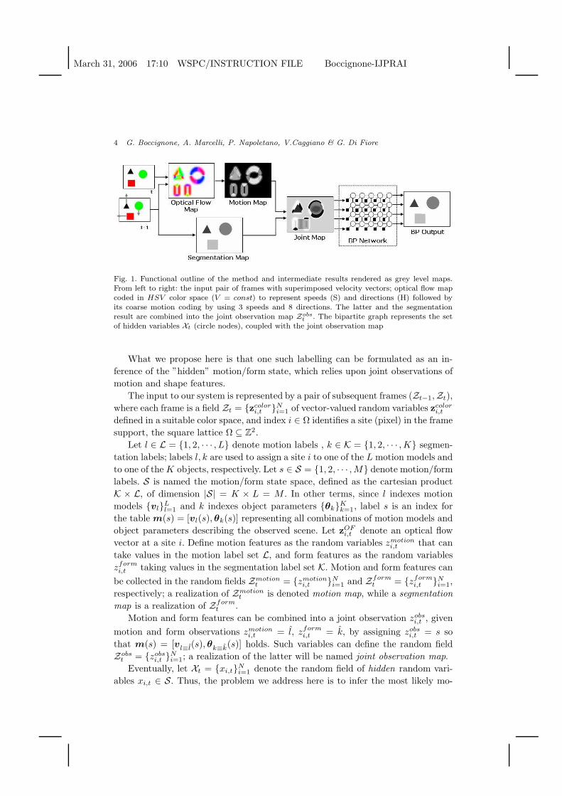
Fig. 1. Functional outline of the method and intermediate results rendered as grey level maps.From left to right: the input pair of frames with superimposed velocity vectors; optical flow mapcoded in HSV color space (V = const) to represent speeds (S) and directions (H) followed byits coarse motion coding by using 3 speeds and 8 directions. The latter and the segmentationresult are combined into the joint observation map Zobs

t. The bipartite graph represents the set

of hidden variables Xt (circle nodes), coupled with the joint observation map

What we propose here is that one such labelling can be formulated as an in-

ference of the ”hidden” motion/form state, which relies upon joint observations of

motion and shape features.

The input to our system is represented by a pair of subsequent frames (Zt−1,Zt),

where each frame is a field Zt = zcolori,t N

i=1 of vector-valued random variables zcolori,t

defined in a suitable color space, and index i ∈ Ω identifies a site (pixel) in the frame

support, the square lattice Ω ⊆ Z2.

Let l ∈ L = 1, 2, · · · , L denote motion labels , k ∈ K = 1, 2, · · · ,K segmen-

tation labels; labels l, k are used to assign a site i to one of the L motion models and

to one of theK objects, respectively. Let s ∈ S = 1, 2, · · · ,M denote motion/form

labels. S is named the motion/form state space, defined as the cartesian product

K × L, of dimension |S| = K × L = M . In other terms, since l indexes motion

models vlLl=1 and k indexes object parameters θk

Kk=1, label s is an index for

the table m(s) = [vl(s),θk(s)] representing all combinations of motion models and

object parameters describing the observed scene. Let zOFi,t denote an optical flow

vector at a site i. Define motion features as the random variables zmotioni,t that can

take values in the motion label set L, and form features as the random variables

zformi,t taking values in the segmentation label set K. Motion and form features can

be collected in the random fields Zmotiont = zmotion

i,t Ni=1 and Zform

t = zformi,t N

i=1,

respectively; a realization of Zmotiont is denoted motion map, while a segmentation

map is a realization of Zformt .

Motion and form features can be combined into a joint observation zobsi,t , given

motion and form observations zmotioni,t = l, zform

i,t = k, by assigning zobsi,t = s so

that m(s) = [vl≡l(s),θk≡k(s)] holds. Such variables can define the random field

Zobst = zobs

i,t Ni=1; a realization of the latter will be named joint observation map.

Eventually, let Xt = xi,tNi=1 denote the random field of hidden random vari-

ables xi,t ∈ S. Thus, the problem we address here is to infer the most likely mo-

March 31, 2006 17:10 WSPC/INSTRUCTION FILE Boccignone-IJPRAI

Bayesian propagation for perceiving moving objects 5

tion/form state Xt on the basis of the joint observation Zobst . The method can be

summarized in the following steps.

For each pair of subsequent frames (Zt−1,Zt):

(1) Compute optical flow field zOFi,t N

i=1. Obtain motion map Zmotiont by as-

signing to each site i the most probable velocity model as zmotioni,t =

argmaxlp(zOFi,t |l,vl).

(2) Compute the form map Zformt by assigning to each site i, z

formi,t =

argmaxkp(zcolori,t |k,µk,Σk).

(3) Given Zmotiont and Zform

t , compute the joint map Zobst by assigning to each

site i the state zobsi,t = s consistent with motion and form observations at that

site.

(4) Use a loopy Belief Propagation algorithm to infer the most likely ”hidden” map

Xt, through the joint density p(Xt,Zobst ) represented via a graphical model with

a pairwise Markov network topology.

Note that step (1) results in a quantization of the motion field, while step (2) per-

forms a segmentation of the observed scene. Eventually, the BP step integrates such

information by taking into account spatial constraints and thus inferring a coherent

moving form. Intermediate results of the different processing steps are illustrated

in Fig. 1 by using a simple example of synthetic moving objects: namely, a black

triangle, a green disk and a red square that are moving in different directions and

with different speeds. The same example will be exploited throughout this section

to detail the proposed approach. It is easy to note that, even in this ”toy” exam-

ple, features derived from motion analysis, although quantized, and segmentation

are per se unreliable for characterizing a moving form, and the joint map itself

could not be straightforwardly used for such purpose. This remark motivates the

introduction of an inference step performed by resorting to Belief Propagation.

3. Computation of motion features

Results presented in Fig. 1 (cfr. the optical flow map) give evidence of the gen-

eral problem that optical flow fields derived from multiple motions usually display

discontinuities (motion edges) and sparseness. This pose a sever issue on direct

exploitation of the flow map to characterize motion at the object level18,17.

To overcome such drawback, we assume that the input to the network should

capture tuning properties of MT neurons in terms of their velocity selectivity20,7.

Rather than model all of the details in the neural circuits that might be responsible

to achieve such tuned responses7, we instead use a simpler system (similarly to

Ref. 20) to compute a quantized velocity encoding (Fig. 2). To this end, the initial

velocity flow field zOFt,i N

i=1 is obtained by using Horn-Shunk algorithm10; an ex-

ample is provided in Fig. 1. Then, we assume that a number L of possible velocities

(motion models) exists, each characterized by different speed and direction. The

latter are represented by a finite set of locations Λ = vlLl=1 in a velocity reference

March 31, 2006 17:10 WSPC/INSTRUCTION FILE Boccignone-IJPRAI

6 G. Boccignone, A. Marcelli, P. Napoletano, V.Caggiano & G. Di Fiore

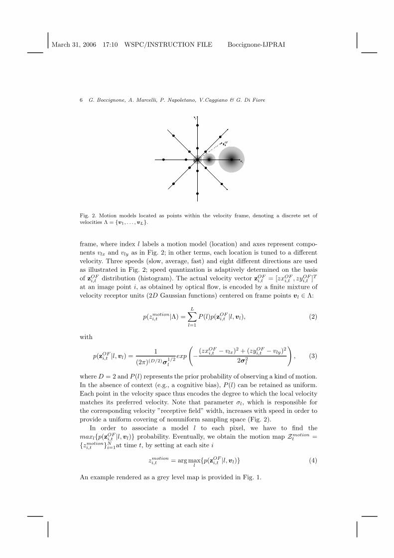
Fig. 2. Motion models located as points within the velocity frame, denoting a discrete set ofvelocities Λ = v1, . . . , vL.

frame, where index l labels a motion model (location) and axes represent compo-

nents vlx and vly as in Fig. 2; in other terms, each location is tuned to a different

velocity. Three speeds (slow, average, fast) and eight different directions are used

as illustrated in Fig. 2; speed quantization is adaptively determined on the basis

of zOFi,t distribution (histogram). The actual velocity vector zOF

i,t = [zxOFi,t , zy

OFi,t ]T

at an image point i, as obtained by optical flow, is encoded by a finite mixture of

velocity receptor units (2D Gaussian functions) centered on frame points vl ∈ Λ:

p(zmotioni,t |Λ) =

L∑

l=1

P (l)p(zOFi,t |l,vl), (2)

with

p(zOFi,t |l,vl) =

1

(2π)(D/2)σ1/2l

exp

(−

(zxOFi,t − vlx)2 + (zyOF

i,t − vly)2

2σ2l

), (3)

whereD = 2 and P (l) represents the prior probability of observing a kind of motion.

In the absence of context (e.g., a cognitive bias), P (l) can be retained as uniform.

Each point in the velocity space thus encodes the degree to which the local velocity

matches its preferred velocity. Note that parameter σl, which is responsible for

the corresponding velocity ”receptive field” width, increases with speed in order to

provide a uniform covering of nonuniform sampling space (Fig. 2).

In order to associate a model l to each pixel, we have to find the

maxlp(zOFi,t |l,vl) probability. Eventually, we obtain the motion map Zmotion

t =

zmotioni,t N

i=1at time t, by setting at each site i

zmotioni,t = argmax

lp(zOF

i,t |l,vl) (4)

An example rendered as a grey level map is provided in Fig. 1.

March 31, 2006 17:10 WSPC/INSTRUCTION FILE Boccignone-IJPRAI

Bayesian propagation for perceiving moving objects 7

4. Computation of form features

Initial form features are derived through segmentation, that is by assigning a label

k to each site i, given the observed data zcolori,t = [Yi,t, Cbi,t, Cri,t]

T in the Y CbCr

color space. Segmentation is accomplished via Diffused Expectation Maximisation

(DEM)3, a variant of the expectation maximisation (EM) algorithm. The method

models an image/frame as a finite mixture, where each mixture component corre-

sponds to a region class and uses a maximum likelihood approach to estimate the

parameters of each class, via the EM algorithm, coupled with anisotropic diffusion

on classes, in order to account for the spatial dependencies among pixels.

To this end, the probabilistic model is assumed to be the mixture

p(zcolori,t |Θ) =

K∑

k=1

P (k)p(zcolori,t |k,θk), (5)

where Θ = θk, kKk=1 and θk = (µk,Σk) is the vector of the parameters (mean

vectors and covariance matrices) associated to label k ∈ K. Each label k defines a

particular region/form, and p(zcolori,t |k,θk) are multivariate gaussians

p(zcolori,t |k,µk,Σk) =

exp(− 12 (zcolor

i,t − µk)TΣ−1k (zcolor

i,t − µk)

(2π)(D/2)|Σk|1/2, (6)

weighted by mixing proportions P (k). Note that, we can consider the covariance

matrices being diagonal because of the choice of the Y CrCb color space, and,

furthermore we assume K fixed, in that we are not concerned here with the problem

of model selection. Parameters of each object are estimated via DEM 3. After

the parameter estimation stage has been completed, segmentation is achieved by

assigning to each site i, the label k for which maxkp(zcolori,t |k,µk,Σk) holds:

zformi,t = arg max

kp(zcolor

i,t |k,µk,Σk) (7)

The assignment produces the segmentation map at time t, Zformt (see Fig. 1).

5. Inference of moving forms via Belief Propagation

At this stage, local observations of both motion and form features are available at

each point of the observed scene, and collected into the motion and segmentation

maps, Zmotiont and Zform

t . Then, the integration of such features into consistent

percepts can be formulated in terms of the inference, for each point i, of the most

likely joint motion/form state xi,t, given Zmotiont and Zform

t .

Here we show how such inference can be accomplished through Belief

Propagation19,14. BP algorithms can best be understood by imagining that each

node in a Markov net, which is responsible for a local observation, communicates

by ”messages” with other connected nodes about what their beliefs should be. The

messages converge after a finite number of steps, when each node has correctly

computed its own belief b(xi,t) (posterior distribution).

March 31, 2006 17:10 WSPC/INSTRUCTION FILE Boccignone-IJPRAI

8 G. Boccignone, A. Marcelli, P. Napoletano, V.Caggiano & G. Di Fiore

Formally, we want to estimate the joint probability p(Xt,Zformt ,Zmotion

t ), where

Xt = xi,tNi=1 is the field of hidden random variables xi,t taking values in S. To

this end, we use the joint observation Zobst = zobs

i,t Ni=1 derived from the pair

(Zcolort ,Zmotion

t ) as described in Section 2, by assigning zobsi,t = s so that m(s) =

[vl≡l(s),θk≡k(s)] holds, and where l and k are consistent with motion and form

observation zmotioni,t = l, zform

i,t = k at the same site i. For what concerns object

parameters, we only retain the vector mean µk and omit covariance Σk. Also, each

motion model vl is represented in terms of speed and direction (vl, ρl). Thus label

s provides access to features (vl(s), ρl(s),µk(s)) in the look-up table m(s), namely

the quantized speed and direction of motion, and average color of the k-th region.

Also it is worth remarking that at this stage, the state space S is dynamically

reduced to those state/models that have been actually employed; in other terms

the cardinality of the space is |S| = K × L = M , where M 6 M .

The random field Zobst represents the set of observed variables to estimate the

density p(Xt,Zformt ,Zmotion

t ) via p(Xt,Zobst ), where Zmotion

t ,Zformt ,Zobs

t ,Xt share

the same support (topology), the connected grid Ω. Then, coupling between motion

and form modules can be represented via a graphical model, with a pairwise Markov

network topology as illustrated in Fig. 1. Define E the corresponding set of edge

indexes of the set Xt; two nodes, say i, j ∈ Ω are correlated if and only if the index

associated to the edge, in this case (i, j), exists in the set E. The overall or ”joint”

probability that defines a generative model on this graph is

p(Xt,Zobst ) =

1

ZQ

∏

(i,j)∈E

ψi,j(xi,t, xj,t)

N∏

i=1

φi(xi,t, zobsi,t ), (8)

where φi(xi,t, zobsi,t ) represents the compatibility function between xi,t and zobs

i,t , also

called the evidence for xi,t, and ψi,j(xi,t, xj,t) represents the compatibility function

between xi,t and xj,t, also called the interaction between i and j 19. The main goal is

to find the belief b(xi,t) = p(xi,t,Zobst ), that is the marginal probability distribution

of each node to be in a state xi,t.

The belief at each node could be obtained by marginalizing p(Xt,Zobst ); unfor-

tunately, marginalization is not an efficient method because exponential in the size

of the graph. To turn an exponential inference computation into one which is linear,

Belief Propagation (BP) algorithms were proposed19, that calculate beliefs by local

message-passing where each message is defined as 19,?:

mij(xj,t) = β∑

xi,t∈S

ψj,i(xj,t, xi,t)φ(xi,t, zobsi,t ) ×

∏

s∈Γ(i)\j

msi(xi,t)

, (9)

where Γ(i) , j|(i, j) ∈ E defines the neighborhood of node i. For graphs which

are acyclic the BP algorithm gives the exact marginal probability distribution 14

b(xi,t) = p(xi,t,Zobst ) = αφ(xi,t, z

obsi,t )

∏

j∈Γ(i)

mji(xi,t), (10)

March 31, 2006 17:10 WSPC/INSTRUCTION FILE Boccignone-IJPRAI

Bayesian propagation for perceiving moving objects 9

where α is a normalization constant, and∑

xi,t∈S b(xi,t) = 1. Notwithstanding the

grid topology we are exploiting, strong empirical results and recent theoretical work

provide support for a very simple approximation: applying the propagation rules

above even in a network with loops5. Yet, we have to solve the problem of designing

suitable compatibility functions φ and ψ.

5.1. Compatibility functions

In order to model compatibility functions φ(xi,t, zobsi,t ) and ψ(xi,t, xj,t), recall that,

according to the discrete formulation of the BP algorithm we have provided,

both the observations zobsi,t and the hidden states xi,t take values within the set

S labelling the M form/motion models. Compatibilities can be determined5 as

φ(xi,t, zobsi,t ) ∝ p(xi,t, z

obsi,t ), ψ(xi,t, xj,t) ∝ p(xi,t, xj,t), that is in both cases, due to

our representation, as p(s, s′), s, s′ ∈ S indexing a pair of models. In the vein of

Ref. 5 we assume a Gaussian penalty

p(s, s′) =

3∏

q=1

exp

(−

(mq(s) −mq(s′))

2

2σ2q

), (11)

where mq(s) represents one of three fields of table m(s) = [vl(s), ρl(s),µk(s)] in-

dexed by s and σ2q is a penalty parameter.

By providing initialization and compatibility functions obtained as described

above, the BP algorithm iterates message passing among nodes (see Eq. 9) until

convergence to a final state map Xt (Fig. 1). Convergence condition6 is obtained as1N

∑Ni=1 |b(xi,t) − b(xi,t−1)| < ǫ, where ǫ is experimentally determined (ǫ = 0.004).

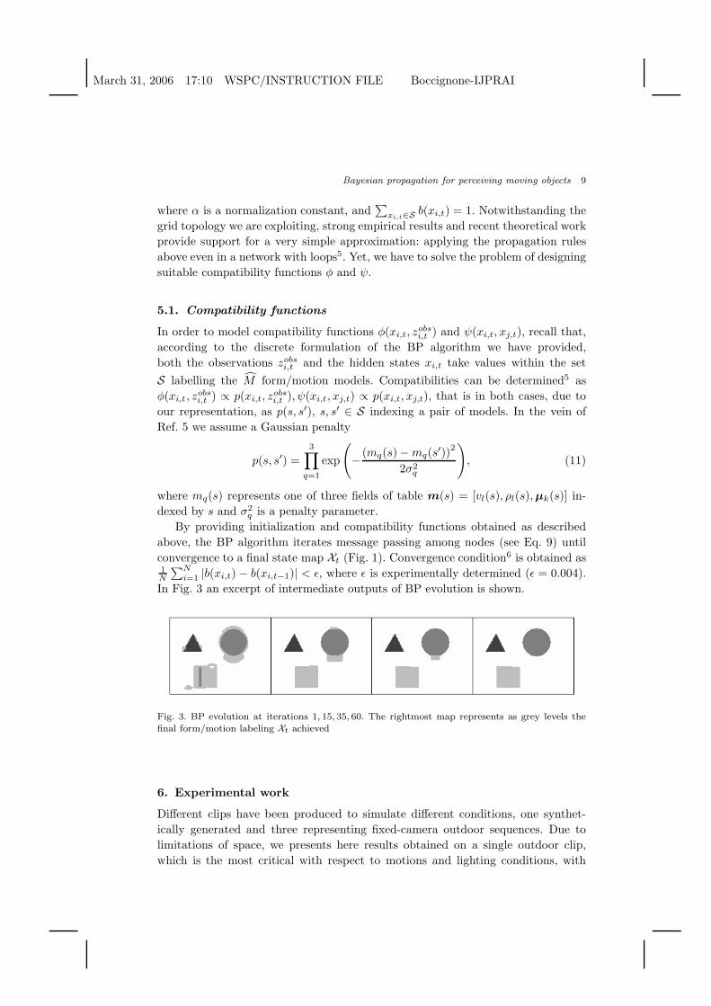
In Fig. 3 an excerpt of intermediate outputs of BP evolution is shown.

Fig. 3. BP evolution at iterations 1, 15, 35, 60. The rightmost map represents as grey levels thefinal form/motion labeling Xt achieved

6. Experimental work

Different clips have been produced to simulate different conditions, one synthet-

ically generated and three representing fixed-camera outdoor sequences. Due to

limitations of space, we presents here results obtained on a single outdoor clip,

which is the most critical with respect to motions and lighting conditions, with

March 31, 2006 17:10 WSPC/INSTRUCTION FILE Boccignone-IJPRAI

10 G. Boccignone, A. Marcelli, P. Napoletano, V.Caggiano & G. Di Fiore

people walking at different distances from the camera, at different speeds and di-

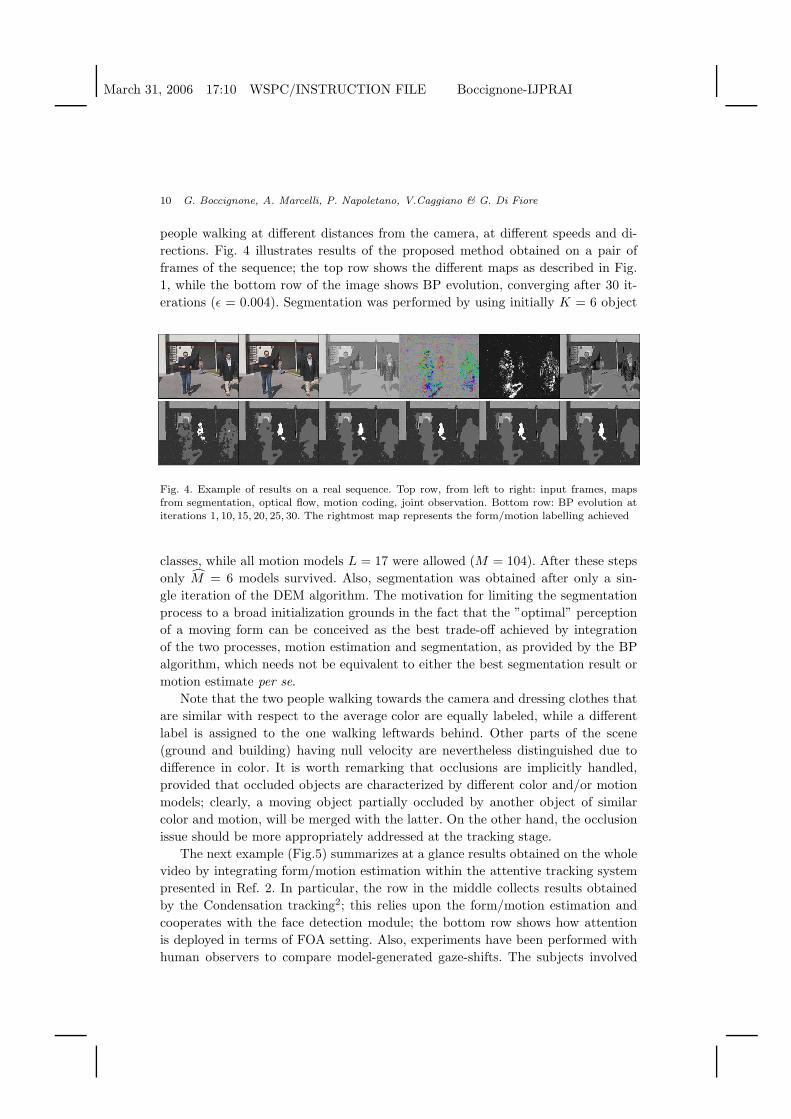
rections. Fig. 4 illustrates results of the proposed method obtained on a pair of

frames of the sequence; the top row shows the different maps as described in Fig.

1, while the bottom row of the image shows BP evolution, converging after 30 it-

erations (ǫ = 0.004). Segmentation was performed by using initially K = 6 object

Fig. 4. Example of results on a real sequence. Top row, from left to right: input frames, mapsfrom segmentation, optical flow, motion coding, joint observation. Bottom row: BP evolution atiterations 1, 10, 15, 20, 25, 30. The rightmost map represents the form/motion labelling achieved

classes, while all motion models L = 17 were allowed (M = 104). After these steps

only M = 6 models survived. Also, segmentation was obtained after only a sin-

gle iteration of the DEM algorithm. The motivation for limiting the segmentation

process to a broad initialization grounds in the fact that the ”optimal” perception

of a moving form can be conceived as the best trade-off achieved by integration

of the two processes, motion estimation and segmentation, as provided by the BP

algorithm, which needs not be equivalent to either the best segmentation result or

motion estimate per se.

Note that the two people walking towards the camera and dressing clothes that

are similar with respect to the average color are equally labeled, while a different

label is assigned to the one walking leftwards behind. Other parts of the scene

(ground and building) having null velocity are nevertheless distinguished due to

difference in color. It is worth remarking that occlusions are implicitly handled,

provided that occluded objects are characterized by different color and/or motion

models; clearly, a moving object partially occluded by another object of similar

color and motion, will be merged with the latter. On the other hand, the occlusion

issue should be more appropriately addressed at the tracking stage.

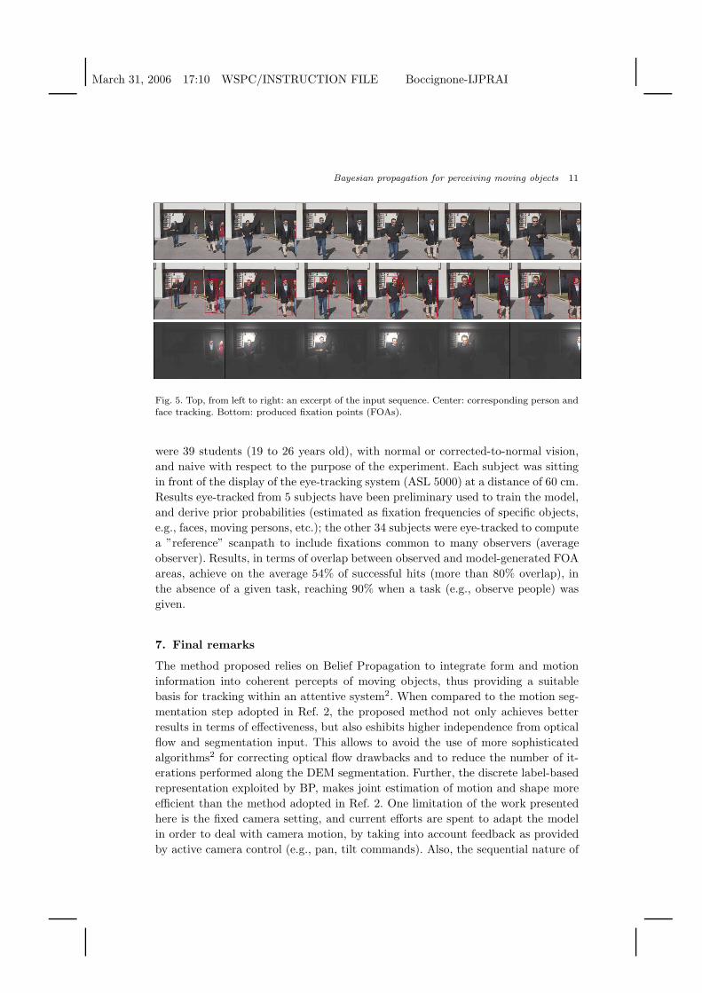
The next example (Fig.5) summarizes at a glance results obtained on the whole

video by integrating form/motion estimation within the attentive tracking system

presented in Ref. 2. In particular, the row in the middle collects results obtained

by the Condensation tracking2; this relies upon the form/motion estimation and

cooperates with the face detection module; the bottom row shows how attention

is deployed in terms of FOA setting. Also, experiments have been performed with

human observers to compare model-generated gaze-shifts. The subjects involved

March 31, 2006 17:10 WSPC/INSTRUCTION FILE Boccignone-IJPRAI

Bayesian propagation for perceiving moving objects 11

Fig. 5. Top, from left to right: an excerpt of the input sequence. Center: corresponding person andface tracking. Bottom: produced fixation points (FOAs).

were 39 students (19 to 26 years old), with normal or corrected-to-normal vision,

and naive with respect to the purpose of the experiment. Each subject was sitting

in front of the display of the eye-tracking system (ASL 5000) at a distance of 60 cm.

Results eye-tracked from 5 subjects have been preliminary used to train the model,

and derive prior probabilities (estimated as fixation frequencies of specific objects,

e.g., faces, moving persons, etc.); the other 34 subjects were eye-tracked to compute

a ”reference” scanpath to include fixations common to many observers (average

observer). Results, in terms of overlap between observed and model-generated FOA

areas, achieve on the average 54% of successful hits (more than 80% overlap), in

the absence of a given task, reaching 90% when a task (e.g., observe people) was

given.

7. Final remarks

The method proposed relies on Belief Propagation to integrate form and motion

information into coherent percepts of moving objects, thus providing a suitable

basis for tracking within an attentive system2. When compared to the motion seg-

mentation step adopted in Ref. 2, the proposed method not only achieves better

results in terms of effectiveness, but also eshibits higher independence from optical

flow and segmentation input. This allows to avoid the use of more sophisticated

algorithms2 for correcting optical flow drawbacks and to reduce the number of it-

erations performed along the DEM segmentation. Further, the discrete label-based

representation exploited by BP, makes joint estimation of motion and shape more

efficient than the method adopted in Ref. 2. One limitation of the work presented

here is the fixed camera setting, and current efforts are spent to adapt the model

in order to deal with camera motion, by taking into account feedback as provided

by active camera control (e.g., pan, tilt commands). Also, the sequential nature of

March 31, 2006 17:10 WSPC/INSTRUCTION FILE Boccignone-IJPRAI

12 G. Boccignone, A. Marcelli, P. Napoletano, V.Caggiano & G. Di Fiore

video analysis is not taken into account here, while it could be embedded within

the method in order to exploit at frame Zt+1, estimates of parameters computed on

Zt6. On-going research is investigating a possible generalization via nonparametric

BP techniques13.

References

1. S. Amari, “Information geometry of the em and em algorithms for neural networks,”Neur. Networks 8 (1995) 1379–1408

2. G. Boccignone,V. Caggiano, G. Di Fiore , A. Marcelli, P. Napoletano, “A Bayesianapproach to situated vision,” Brain, Vision and Artificial Intelligence 2005, LNCS

3704, eds. M de Gregorio, V. Di Maio, M. Frucci, C. Musio, 2005, pp 367-3763. G. Boccignone, M. Ferraro, P. Napoletano, “Diffused expectation maximisation for

image segmentation,” Electronics Letters 40 (2004) 1107–11084. K.H. Britten: “Motion Perception: How are moving images segmented?,” Current Bi-

ology 9 (1999) 728–7305. W.T.Freeman, E.C. Pasztor, O.T. Carmichael: “Learning Low-Level Vision,” Int. J.

of Computer Vision, 40 (2000) 25–476. B.J. Frey, N. Jojic, “A Comparison of Algorithms for Inference and Learning in Prob-

abilistic Graphical Models, IEEE Trans. on PAMI, 27 (2005) 1392–14167. S. Grossberg, E. Mingolla, C. Pack, “A neural model of motion processing and visual

navigation by cortical area MST,” Cerebral Cortex (1999) 9 878–895.8. M.M. Hayhoe, D.H. Ballard, D. Bensinger, “Task constraints in visual working mem-

ory,” Vision Research 38 (1998) 125–1379. H. Helmholtz. Physiological Optics, vol III: The Perception of Vision. Optical Society

of America , Rochester, NY., 192510. B.K.P. Horn, Robot Vision. MIT Press, Cambridge,MA 198611. M. Isard, A. Blake, “Condensation-conditional density propagation for visual track-

ing,” Int. J. of Computer Vision 29 (1998) 5–2812. D.C. Knill, D. Kersten and A. Yuille, ”A Bayesian formulation of visual perception”.

In: Perception as Bayesian Inference , Knill, D.C, Richards, W. (eds), CambridgeUniversity Press, 1996.

13. T.S. Lee, D. Mumford, “Hierarchical bayesian inference in the visual cortex,” J. Opt.

Soc. Am. A 20 (2003) 1434–144814. J. Pearl, Probabilistic reasoning in intelligent systems:networks of plausible inference.

Morgan Kaufmann (1988)15. Z. Pylyshyn, “Situating vision in the world,” Trends in Cognitive Sciences 4 (2000)

197–20716. J. E. Raymond: “Attentional modulation of visual motion perception,” Trends Cog.

Sciences 4 (2000) 42–5017. N. Vasconcelos, A. Lippman, “Empirical bayesian motion segmentation,” IEEE Trans.

on PAMI 23 (2001) 217–22018. Y. Weiss, E. Adelson, “A unified mixture framework for motion segmentation: incor-

porating spatial coherence and estimating the number of models,” Proc. IEEE Conf.

Comp. Vision Patt. Recognition, IEEE Computer Soc. Press, 1996, pp 321–32619. J.S. Yedidia, W.T. Freeman, Y. Weiss, “Understanding belief propagation and its

generalizations,” Exploring artificial intelligence in the new millennium, Morgan Kauf-mann, San Francisco, CA, 2003, pp 239–269

20. R. S. Zemel, T.J. Sejnowski: “A Model for Encoding Multiple Object Motions and

March 31, 2006 17:10 WSPC/INSTRUCTION FILE Boccignone-IJPRAI

Bayesian propagation for perceiving moving objects 13

Self-Motion in Area MST of Primate Visual Cortex,” The J. of Neuroscience (1998)18 531–547

Giuseppe Boccignone

received the Laurea de-gree in Theoretical Physicsfrom the University ofTorino, Italy, in 1985.He has been with OlivettiCorporate Research, Ivrea,chief researcher of theComputer Vision andArtificial Intelligence Lab

at CRIAI Naples, Research Consultant at Re-search Labs of Bull HN, Milan, Italy. In 1994,he joined as Assistant Professor the Depart-ment of Electrical and Information Engineer-ing, University of Salerno, Italy, where he cur-rently is an Associate Professor of ComputerScience. He is a member of the IEEE, IEEEComputer Society and IAPR. His researchinterests lie in active vision and theoreticalmodels for computational vision.

Vittorio Caggiano re-ceived the Laurea de-gree in Electronic En-gineering from the Uni-versity of Salerno, Italy,in 2004. He currently isa Ph.D. student in com-puter engineering at theUniversity of Naples”Federico II”, Italy. His

research interests lie in active vision, biologi-cal vision, medical imaging, image and videodatabases.

Gianluca Di Fiore re-ceived the Laurea de-gree in Computer En-gineering from the Uni-versity of Naples Fed-erico II, Naples, Italy,in 2003. Currently, he

is a Research Consul-tant at CoRiTel Labs,Salerno,Italy. His re-

search interests lie in video analysis and com-pression, software engineering.

Angelo Marcelli re-ceived the M.Sc. degreein Electronic Engineer-ing (cum laude) and thePh.D. in Electronic andComputer Engineeringboth from the Univer-sity of Napoli ”FedericoII”, Italy, in 1983 and1987, respectively. From

1987 to 1989, he was chief researcher of theComputer Vision and Artificial IntelligenceLab at CRIAI, Napoli, Italy, where he alsofounded and directed the Italy-Russian Lab-oratory for Image Analysis and Processing.From 1989 to 1992, he has held a Researcherposition at Department of Computer and Sys-tem Engineering, School of Engineering, Uni-versity of Napoli ”Federico II”. Since 1998,he has been with the Department of Electri-cal and Information Engineering of the Uni-versity of Salerno, where he is currently As-sociate Professor. Dr. Marcelli serves as AreaEditor for the International Journal of Docu-

ment Analysis and Recognition. He is a mem-ber of the IEEE, IEEE Computer Society,IEEE Systems, Man and Cybernetics Soci-ety, IEEE Education Society, IAPR. He isthe President-elect of International Grapho-nomics Society. His current research interestinclude handwriting recognition, theory andapplication of evolutionary algorithms, activevision model and natural computation.

Paolo Napoletano re-ceived the Laurea de-gree in Telecommunica-tion Engineering fromthe University of NaplesFederico II, Italy, in2003. He currently isa Ph.D. student in In-formation Engineeringat the University of

Salerno, Italy. He is a student member of theIEEE, IEEE Computer Society. His researchinterests lie in active vision, theoretical mod-els for computational vision, medical imagingand image processing.