Physica D 206 (2005) 180–212 Localized activity patterns in two-population neuronal networks Patrick Blomquist ∗ , John Wyller, Gaute T. Einevoll Department of Mathematical Sciences and Technology, Norwegian University of Life Sciences, P.O. Box 5003, N-1432 ˚ As, Norway Received 9 November 2004; received in revised form 28 April 2005; accepted 3 May 2005 Available online 2 June 2005 Communicated by A. Doelman Abstract We investigate a two-population neuronal network model of the Wilson–Cowan type with respect to existence of localized stationary solutions (“bumps”) and focus on the situation where two separate bump solutions (one narrow pair and one broad pair) exist. The stability of the bumps is investigated by means of two different approaches: The first generalizes the Amari approach, while the second is based on a direct linearization procedure. A classification scheme for the stability problem is formulated, and it is shown that the two approaches yield the same predictions, except for one notable exception. The narrow pair is generically unstable, while the broad pair is stable for small and moderate values of the relative inhibition time. At a critical relative inhibition time the broad pair is typically converted to stable breathers through a Hopf bifurcation. In our numerical example the broad pulse pair remains stable even when the inhibition time constant is three times longer than the excitation time constant. Thus, our model results do not support the claim that slow excitation mediated by, e.g., NMDA-receptors is needed to allow stable bumps. © 2005 Elsevier B.V. All rights reserved. PACS: 87.19.La; 89.75.Kd; 02.30.Rz Keywords: Pattern formation; Integro-differential equations; Short term memory; Neuroscience 1. Introduction Experimental observations have established persistent neuronal activity in prefrontal cortex as a neural process underlying short-term, working memory (for a review, see Ref. [1]). In particular, localized persistent activity, or “bumps”, in cortical networks may serve as memory storage. Numerous modelling studies have examined ∗ Corresponding author. Tel.: +47 6496 5427; fax: +47 6496 5401. E-mail addresses: [email protected] (P. Blomquist), [email protected] (J. Wyller), [email protected] (G.T. Einevoll) 0167-2789/$ – see front matter © 2005 Elsevier B.V. All rights reserved. doi:10.1016/j.physd.2005.05.004

Welcome message from author
This document is posted to help you gain knowledge. Please leave a comment to let me know what you think about it! Share it to your friends and learn new things together.
Transcript
Physica D 206 (2005) 180–212
Localized activity patterns in two-populationneuronal networks
Patrick Blomquist∗, John Wyller, Gaute T. Einevoll
Department of Mathematical Sciences and Technology, Norwegian University of Life Sciences,P.O. Box 5003, N-1432̊As, Norway
Received 9 November 2004; received in revised form 28 April 2005; accepted 3 May 2005Available online 2 June 2005
Communicated by A. Doelman
Abstract
We investigate a two-population neuronal network model of the Wilson–Cowan type with respect to existence of localizedstationary solutions (“bumps”) and focus on the situation where two separate bump solutions (one narrow pair and one broadpair) exist. The stability of the bumps is investigated by means of two different approaches: The first generalizes the Amariapproach, while the second is based on a direct linearization procedure. A classification scheme for the stability problem isformulated, and it is shown that the two approaches yield the same predictions, except for one notable exception. The narrow pairis generically unstable, while the broad pair is stable for small and moderate values of the relative inhibition time. At a criticalrelative inhibition time the broad pair is typically converted to stable breathers through a Hopf bifurcation. In our numericalexample the broad pulse pair remains stable even when the inhibition time constant is three times longer than the excitation timeconstant. Thus, our model results do not support the claim that slow excitation mediated by, e.g., NMDA-receptors is needed toallow stable bumps.© 2005 Elsevier B.V. All rights reserved.
PACS:87.19.La; 89.75.Kd; 02.30.Rz
Keywords:Pattern formation; Integro-differential equations; Short term memory; Neuroscience
1. Introduction
Experimental observations have established persistent neuronal activity in prefrontal cortex as a neural processunderlying short-term, working memory (for a review, see Ref.[1]). In particular, localized persistent activity,or “bumps”, in cortical networks may serve as memory storage. Numerous modelling studies have examined
∗ Corresponding author. Tel.: +47 6496 5427; fax: +47 6496 5401.E-mail addresses:[email protected] (P. Blomquist), [email protected] (J. Wyller), [email protected] (G.T. Einevoll)
0167-2789/$ – see front matter © 2005 Elsevier B.V. All rights reserved.doi:10.1016/j.physd.2005.05.004
P. Blomquist et al. / Physica D 206 (2005) 180–212 181
the existence and stability of such bumps, and both firing-rate and spiking-neuron models have been considered[2–27]. An excellent and current review of bumps in neural firing-rate models (as well as waves and other patterns)is provided by Ref.[27].
In an early study Amari[3] proved analytically the existence and stability of such bumps in a simplified ratemodel of the lateral inhibition (LI) type in one spatial dimension,
ut(x, t) = −u(x, t) +∫ ∞
−∞ω(x − x′)P(u(x′, t)) dx′ + s(x, t) + h (1)
Hereu(x, t) denotes the “synaptic input” to a neural element at positionx and timet, andut(x, t) is the corre-sponding time derivative. The non-negative functionP(u) gives the firing rate of a neuron with inputu. The functions(x, t) represents a variable external input while the parameterh represents a constant external input applied uni-formly to all neurons. The synaptic connectivity functionω(x) determines the coupling between the neurons, andin LI networks this typically has a characteristic “Mexican-hat shape”: nearby neurons excite each other (recurrentexcitation) while more distant neurons inhibit each other (lateral inhibition). For the case where the firing-ratefunctionP(u) is chosen to be the Heaviside step function, Amari[3] proved the existence of stable bumps in sucha LI network; stable bumps are sustained by local recurrent excitation and localized by lateral inhibition.
More recent studies have investigated existence and stability of a variety of bump types in generalized Amari-type models where different synaptic coupling functionsω(x) and firing-rate functionsP(u) have been considered[10,15,16,18,21,23,24]. Effects of axo-dendritic synaptic processing have also been studied[16].
In LI-models of the Amari type the spatially extended inhibition models in a simplified way the excitation ofand consequtive return inhibition from inhibitory interneurons surrounding the excitatory model population. Thisone-population model for excitatory neurons can be seen to correspond to a two-population model incorporating anadditional inhibitory population, in the limit where the inhibitory time constant goes to zero[13]. A crucial questionis thus whether bumps found to be stable in “instantaneous-inhibition” Amari models are stable also when modelsincorporating more realistic inhibitory delays are considered[13].
Recent modelling studies with spiking-neuron networks have focused on requirements for bump stability inthe context of working memory. Compte et al.[9] considered a two-population network of leaky integrate-and-fireneurons and found that the recurrent synaptic excitation should primarily be mediated by the slower NMDA-receptorsto achieve stability; with the faster AMPA-receptors dominating, the excitation would be too fast compared to theGABAA-mediated inhibition and bump stability would be lost (see also discussions in[1,28]). However, Gutkin etal. [11] found that bump stability could be achieved also with AMPA-receptors when networks based on biologicallymore realistic neuron models were used.
To study the effects of excitation and inhibition times on bump stability in a rate model, one must go beyond theone-population Amari-type model. Pinto and Ermentrout[13] studied the existence and stability of bumps in thefollowing two-population model:
∂tue = −ue +∫ ∞
−∞ωee(x − x′)P(ue(x
′, t) − θ) dx′ −∫ ∞
−∞ωie(x − x′)ui (x
′, t) dx′, (2a)
τ∂tui = −ui +∫ ∞
−∞ωei(x − x′)P(ue(x
′, t) − θ) dx′. (2b)
Hereue(x, t) andui (x, t) represents the synaptic input to an excitatory and an inhibitory neural element re-spectively, andτ the inhibitory time constant (measured relative to the excitatory time constant). Compared to theanalogous two-population model studied by Wilson and Cowan[2] this model (i) neglects a term describing recur-rent inhibition (i→ i) and (ii) assumes a linear firing-rate function for the inhibitory population. These assumptionsallows for a reduction of the two-equation system to a single equation in the mathematical analysis of the existenceand stability of bumps. For their model Pinto and Ermentrout found that the inclusion of the more realistic inhibitorydynamics resulted in a loss of stability. They thus concluded that their work did not support the hypothesis that
182 P. Blomquist et al. / Physica D 206 (2005) 180–212
sustained activity in prefrontal cortex is a result of the dynamics in an LI network (even though it could not be ruledout completely since an attempt to quantify the necessary speed of inhibition to maintain stability was not made).
In the present work we consider the following two-population model,
∂tue = −ue +∫ ∞
−∞ωee(x − x′)Pe(ue(x
′, t) − θe) dx′ −∫ ∞
−∞ωie(x − x′)Pi (ui (x
′, t) − θi ) dx′, (3a)
τ∂tui = −ui +∫ ∞
−∞ωei(x − x′)Pe(ue(x
′, t) − θe) dx′ −∫ ∞
−∞ωii (x − x′)Pi (ui (x
′, t) − θi ) dx′, (3b)
where the dynamics of the excitatory and inhibitory populations are modelled in a symmetric way. We limit ourselvesto the case wherePe andPi are Heaviside step functions, but allow for different threshold valuesθe andθi . Thismodel is analogous to the Wilson–Cowan model[2] where the dynamical variables represent firing rates and not (ashere) synaptic inputs. In Wilson and Cowan[2] numerical examples of stable bumps were given, but a systematicstudy of conditions for the existence and stability of such bumps was not pursued.
We address the same type of questions as in Pinto and Ermentrout[13], i.e., conditions for existence anduniqueness of pairs of spatially symmetric bumps of excitatory and inhibitory neuronal firing for a given set ofthreshold values. In particular we focus on the stability of such bumps, and how it depends on the dynamics of theinhibitory compared to the excitatory population.
In Section2, we formulate the model and show that a general feature is that the solutions are bounded. Section3 is devoted to the study of the existence and uniqueness of stationary symmetric localized pulses, and we provethat such pulses will always exist, i.e., for any choice of synaptic coupling functionsωmn(x) there will always exista set of threshold values (θe, θi ) which assures a stationary pulse. From the proof, it also follows that by choosingappropriate threshold values one can always construct an excitatory pulse accompanied by an arbitrarily narrowinhibitory pulse.
We further investigate the stability of these stationary bumps, using two different approaches: The first approachis based on the formal arguments for stability elaborated by Amari[3] and later used by Pinto and Ermentrout[13].One identifies each stationary pulse with its width. An autonomous dynamical system, which is consistent with themodel equations, for the variation of the width parameters is then derived. The equilibrium point of this systemcorresponds to the widths of the stationary pulses, and it is conjectured that the stability properties of the pulses canbe inferred from the stability properties of the pulse-width equilibrium. The result from this analysis is presentedin Section4. There we find that bumps which are stable for fast inhibition (i.e., not too largeτ) can lose its stabilityat a critical value forτ, τcr, through a Hopf bifurcation.
The second approach given in Section5 is based on a standard linearization procedure with the full set of modelequations and the known stationary bumps as a starting point, in a way identical to the technique presented in[13].Notice that this approach for investigating stability can be generalized to cover the travelling wave stability, usingthe Evans functions approach elaborated in[19].
The results from the two stability-analysis approaches are compared in Section6, and it is shown that Amari’sapproach and the full stability analysis in most, but not all, cases yield the same result. Moreover, we identify aparameter regime where results from the two stability analyses agree and bump stability is lost through a supercriticalHopf bifurcation with the generation of stable breathers.
For the question of whether bumps can be stable in realistic cortical networks and thus function as a substrate forworking memory, the numerical value ofτcr is essential. In Section7 we consider a numerical example whereτcrtypically is around 3. This means that bumps can be stable even if the inhibitory time constant is three times as largeas the excitatory time constant; a requirement that likely can be fulfilled with GABAA mediated inhibition even ifthe recurrent excitation is mediated by AMPA-receptors[1]. This result appears to differ from the correspondingresult for the model studied in[13] where bump stability (in their numerical examples) was lost already for valuesof τ much less than 1. Thus the conclusion regarding the possibility for LI networks to be a substrate for workingmemory appears to be different for these two models.
P. Blomquist et al. / Physica D 206 (2005) 180–212 183
The final Section8 contains a summary and conclusion. InAppendix A we describe the numerical schemeunderlying the computations in Section7, and present some tedious mathematical derivations inAppendix Band C.
2. Model
We generalize the model studied by Pinto and Ermentrout[13] by including a recurrent inhibitory term in theinhibitory equation as well as assuming the coupling from inhibitory to excitatory neurons to be nonlinear. Wealso allow the threshold,θe, for the excitatory population and the threshold,θi , for the inhibitory population to bedifferent. Our model thus reads
∂tue = −ue + ωee∗ Pe(ue − θe) − ωie ∗ Pi (ui − θi ) (4a)
τ∂tui = −ui + ωei ∗ Pe(ue − θe) − ωii ∗ Pi (ui − θi ). (4b)
Here the functionsue = ue(x, t) andui = ui (x, t) model the synaptic input to excitatory and inhibitory neurons,respectively.Pe andPi model the corresponding firing-rate functions. These functions constitute a one-parameterfamily of increasing functions mapping the set of real numbers onto the unit interval, where the parameter involvedmeasures the characteristic variation length of the functions. When the typical width approaches zero, the functionsPm are assumed to approach the Heaviside step functionH. In the present paper we will approximate the firing ratefunctions with the Heaviside step function. The parametersθe andθi play the role as the threshold values for firingof the excitatory and inhibitory populations, respectively, which by assumption may be different.ωmn ∗ f denotesthe convolution integral defined as
(ωmn ∗ f )(x) =∫ ∞
−∞ωmn(x − y)f (y) dy, m, n = e, i (5)
and the functionsωmn are theconnectivity functions, which are assumed to be real valued, positive, bounded,symmetric and to satisfy the normalization condition
∫∞−∞ ωmn(x) dx = 1. In addition, they can generically be
expressed as
ωmn(x) = 1
σmn
· �mn(ξmn), ξmn = x
σmn
(6)
where the parameterσmn describes the spatial extension, i.e.,synaptic footprint, and�(ξmn) is a non-dimensionalscaling function. Finally, the parameterτ is the ratio between the inhibitory and excitatory time constants, whichwe from now on refer to as therelative inhibition time.
As examples on localized connectivity functions of the type(6) we have the Gaussian
�mn(ξmn) = 1√π
exp(−ξ2mn) (7)
and the exponential decay
�mn(ξmn) = 1
2exp(−|ξmn|). (8)
Pinto and Ermentrout[13] address the problem of existence and uniqueness of stationary, symmetric, localizedstationary pulses (“bumps”) as well as stability of these solutions using both a generalized version of the Amariapproach and a direct linearization procedure. In the present paper we will investigate the same type of questions.
184 P. Blomquist et al. / Physica D 206 (2005) 180–212
We first point out a boundedness property for the solutions of the initial value problem of the system. Now, sinceby the conditions imposed onωmn
0 ≤∫ ∞
−∞ωmn(y − x)H(f (y, t) − θm) dy ≤
∫ ∞
−∞ωmn(y − x) dy ≤ 1 (9)
for any functionf, we find the explicit bounds
(Ve(x) + 1)e−t − 1 ≤ ue(x, t) ≤ (Ve(x) − 1)e−t + 1 (10a)
(Vi (x) + 1)e−t/τ − 1 ≤ ui (x, t) ≤ (Vi (x) − 1)e−t/τ + 1 (10b)
for the solution-componentsue andui , where (Ve(x), Vi (x)) is the initial condition of(4). Notice that the results(10) also hold true in the general case of firing rate functions possessing values between 0 and 1. From this resultwe can draw the following conclusion: Since the initial data by assumption obeys
|Ve(x)| ≤ 1, |Vi (x)| ≤ 1 (11)
for all x ∈ R, then
|ue(x, t)| ≤ 1, |ui (x, t)| ≤ 1 (12)
for all x ∈ R, uniformly in t ≥ 0. This property has the following immediate consequences: Ifθm > 1,m = e, i, thenon-locality does not contribute to the time evolution ofum. The global evolution ofum is described as exponentialdecay. For−1 ≤ θm ≤ 1, only the range for whichum(x, t) ≥ θm, contributes to the nonlocal terms. Finally, forθm < −1, all neuronal elements are above threshold and contribute to the nonlocal terms.
The boundednessresult (12)indeed shows that the nonlinear stage of the instabilities we detect by a linearizationprocedure, has to be saturated.
3. Existence and uniqueness of stationary localized solutions
In this section we investigate for our model conditions for existence and uniqueness of pairs of excitatoryand inhibitory symmetric, localized pulses termed “bumps”, by generalizing arguments presented in Pinto andErmentrout[13]. In the following it is assumed that 0< θm ≤ 1 (m = e, i). We conveniently separate the existenceissue from the uniqueness problem.
1. The existence issue is a global problem, and it can be posed as follows: Determine the set of threshold valuesfor firing which produce “bumps”-solutions of(4).
2. The uniqueness problem can be formulated as follows: Suppose we have proven the existence of “bumps”. Thenthe task consists of giving conditions for having a one-to-one correspondence between the threshold values andthe “bumps”. This latter issue turns out to be a local problem.
3.1. Existence theory
We first investigate the possibility of having localized stationary, symmetric solutions of the system(4) andproceed as follows:
1. The firing rate functionsPe andPi are approximated with the Heaviside step function, i.e.,Pm = H (m = e, i).2. The solutions of(4) are assumed to be time-independent, i.e.,ue(x, t) = Ue(x), ui (x, t) = Ui (x) whereUe(x)
andUi (x) are smooth, bounded functions satisfying the following symmetry and limit conditions:
P. Blomquist et al. / Physica D 206 (2005) 180–212 185
• Um(x) = Um(−x), for m = e, i• Um(±∞) = 0, form = e, i• There are unique points denoted bya, b ≥ 0 such thatUe(±a) = θe, Ui (±b) = θi where we have assumed
Ue(x) > θe(< θe), when |x| < a (|x| > a) (13a)
Ui (x) > θi (< θi ), when |x| < b (|x| > b). (13b)
Notice that the conditions imposed above imply that we only consider single bump solutions.The parametersa, b measure the widths of the pulses and hereafter we refer to these parameters as thepulse
widthsof Ue(x) andUi (x). By making use of the stationarity ansatz described above, we now find thatUe(x) andUi (x) can formally be expressed as
Ue(x) =∫ a
−a
ωee(x − x′) dx′ −∫ b
−b
ωie(x − x′) dx′ (14a)
Ui (x) =∫ a
−a
ωei(x − x′) dx′ −∫ b
−b
ωii (x − x′) dx′. (14b)
Now, by combining the remaining assumptions on pulsesUe(x) andUi (x) we find that the conditions which mustbe fulfilled in order to have stationary symmetric solutions read
fe(a, b) = θe (15a)
fi (a, b) = θi (15b)
wherefe andfi are given as
fe(a, b) = Wee(2a) − Wie(a + b) + Wie(a − b) (16a)
fi (a, b) = Wei(a + b) − Wei(b − a) − Wii (2b). (16b)
HereWjk(ξ) is defined as the integral
Wjk(ξ) =∫ ξ
0ωjk(y) dy. (17)
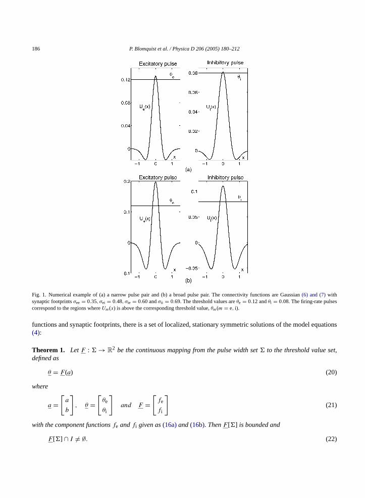
In contrast toωjk which is an even function,Wjk is an odd function.In Fig. 1, we display numerical examples of pulses when the connectivity functions are given as Gaussians(6)
and (7).The key problem now consists of investigating for which threshold valuesθm where 0< θm ≤ 1 (m = e, i) the
system(15)possesses solutions. We conveniently translate this problem into a mapping problem as follows:Introduce the subset! of R
2 as
! = {(a, b)|a ≥ 0, b ≥ 0} (18)
and the unit square
I = 〈0,1] × 〈0,1] (19)
in the (θe, θi )-plane.From now on we refer to! as the pulse width setand I as the threshold value set. We also assume that the
connectivity functionsωmn are continuous for allx ∈ R, except for a possible set of measure zero, which meansthat the vector fieldF : ! → R
2 defines a continuous mapping. Then we show that for all choices of connectivity
186 P. Blomquist et al. / Physica D 206 (2005) 180–212
Fig. 1. Numerical example of (a) a narrow pulse pair and (b) a broad pulse pair. The connectivity functions are Gaussian(6) and (7)withsynaptic footprintsσee = 0.35, σei = 0.48, σie = 0.60 andσii = 0.69. The threshold values areθe = 0.12 andθi = 0.08. The firing-rate pulsescorrespond to the regions whereUm(x) is above the corresponding threshold value,θm(m = e, i).
functions and synaptic footprints, there is a set of localized, stationary symmetric solutions of the model equations(4):
Theorem 1. Let F : ! → R2 be the continuous mapping from the pulse width set! to the threshold value set,
defined as
θ = F (a) (20)
where
a =[a
b
], θ =
[θe
θi
]and F =
[fe
fi
](21)
with the component functionsfe andfi given as(16a)and(16b). ThenF [!] is bounded and
F [!] ∩ I �= ∅. (22)
P. Blomquist et al. / Physica D 206 (2005) 180–212 187
We first prove thatF [!] is bounded. The triangle inequality yields
|fe(a, b)| ≤ |Wee(2a)| + |Wie(a + b)| + |Wie(a − b)| (23a)
|fi (a, b)| ≤ |Wei(a + b)| + |Wei(b − a)| + |Wii (2b)|. (23b)
Now, since the connectivity functions by assumption are symmetric and satisfy the normalization condition, wehave
|Wjk(ξ)| ≤ 1
2. (24)
Hence
|fe(a, b)| ≤ 3
2, |fi (a, b)| ≤ 3
2.
Next, we prove that the intersection between the image setF [!] and the threshold value setI is non-empty. Wefind that the image of the positivea-axis under the mappingF is given as
γ(a) = F (a,0) =[fe(a,0)
fi (a,0)
]=[Wee(2a)
2Wei(a)
]. (25)
The boundary curveγ(a) has the following properties:
γ(0) = 0, γ(a → ∞) = 1
21
. (26)
Moreover, this curve is the graph of a strictly increasing functionG given as
θi = G(θe)
where
θe = Wee(2a), θi = 2Wei(a).
Hence, the image of the positivea-axis is contained in the threshold value setI. Now, since! is simply connectedandF is a continuous mapping, we can conclude that
F [!] ∩ I �= ∅. (27)
This result means that it always exists a subset ofI (which we will termthe set of admissible threshold values) forwhich the system(15)has solutions. For this set of (θe, θi )-values we have localized symmetric pulses. Notice thatthe proof of the theorem shows thatan finite width excitatory pulse may coexist with arbitrarily narrow inhibitorypulse(b → 0).
We will now prove that inhibitory stationary pulses cannot coexist with an arbitrarily narrow excitatory pulses(a → 0) for 0< θm ≤ 1 (m = e, i). This result is represented in terms of the present mathematical terminology asfollows: The intersection of the image of the positiveb-axis, witha = 0, under the mappingF and the thresholdvalue planeI is empty. We prove this result as follows: First, simple computation reveals that
' = F (0, b) =[fe(0, b)
fi (0, b)
]=[
−2Wie(b)
−Wii (2b)
](28)
188 P. Blomquist et al. / Physica D 206 (2005) 180–212
where the components are negative for allb > 0. The image curve' has the properties
'(0) = 0, '(b → ∞) = −1
−1
2
. (29)
Moreover, this image curve is the graph of a strictly increasing function. Hence, the image curve'(b) is totallylocated in the third quadrant, from which it follows that the intersection betweenI and the image curve is empty.Thus, finite width inhibitory pulses cannot coexist with very narrow excitatory pulses (a → 0).
3.2. Uniqueness theory and pulse pair generation
3.2.1. Uniqueness theoryLet us assume that the threshold values (θe, θi ) belong to the admissible subset of threshold values. This means
that (20) possesses a solution which will be denoted by (aeq, beq). We will address the question about uniquenessof the pulse pair solutions. We proceed as follows: Assume that the connectivity functionsωmn are continuous.Then the vector fieldF where the component functions are given by(16), is continuous differentiable. Then, by theinverse function theorem this vector field is locally one-to-one and onto, provided the Jacobian ofF evaluated ataeq = (aeq, beq) is non-singular, i.e.,
det
[∂F
∂a
](aeq) �= 0. (30)
This is clearly a local problem in the sense that the theorem states that there is an open neighborhood ofaeq which is mapped one-to-one and onto an open neighborhood of the threshold values (θe, θi ). Geometrically,the solution of the system(20) satisfying thecondition (30)emerges as a transversal intersection between thelevel curvesfe(a, b) = θe and fi (a, b) = θi . From now on we refer to thecondition (30)as thetransversalitycondition.
3.2.2. Pulse pair generationThe breakdown of the transversalitycondition (30)is connected to the process of the pulse pair generation in a
way which is analogous to the problem of generation of two standing pulses for a given admissible threshold valuethrough a bifurcation process detailed in[13].
We first search for admissible threshold values (θe, θi ) which correspond to a situation where the level curvesfe = θe andfi = θi are tangent to each other. We proceed as follows: One determines positive solutions of thesystem of equations
det
[∂F
∂a
](a, b) = 0 (31a)
fe(a, b) = θe (31b)
for a given set of connectivity functionsωmn and synaptic footprintsσmn whenθe varies through the unit interval.The next step consists of computing the correspondingθi -value by means of the formulafi (a, b) = θi under theconstraint 0< θi ≤ 1. This process generates a separatrix curve in the set of admissible threshold values.
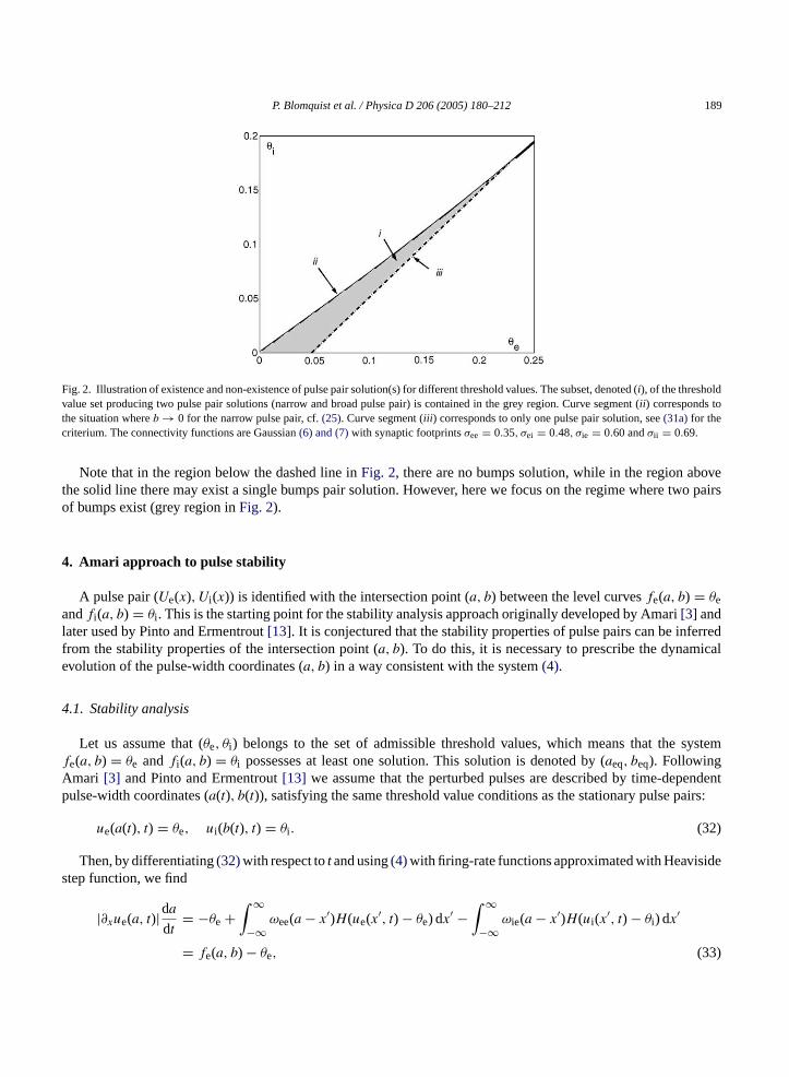
Now, with a proper adjustment of the threshold values around this separatrix curve, we go from a situation withno intersection of the level curvesfe = θe andfi = θi , to a tangent situation as described by(31) and finally endup with two transversal intersection points, from which it follows that we get two pulse pairs locally for a certainrange of threshold values. InFig. 2we see a numerical example of a threshold subset that corresponds to solutionsof (20), where the subset is bounded by(25) and (31a).
P. Blomquist et al. / Physica D 206 (2005) 180–212 189
Fig. 2. Illustration of existence and non-existence of pulse pair solution(s) for different threshold values. The subset, denoted (i), of the thresholdvalue set producing two pulse pair solutions (narrow and broad pulse pair) is contained in the grey region. Curve segment (ii ) corresponds tothe situation whereb → 0 for the narrow pulse pair, cf.(25). Curve segment (iii ) corresponds to only one pulse pair solution, see(31a)for thecriterium. The connectivity functions are Gaussian(6) and (7)with synaptic footprintsσee = 0.35, σei = 0.48, σie = 0.60 andσii = 0.69.
Note that in the region below the dashed line inFig. 2, there are no bumps solution, while in the region abovethe solid line there may exist a single bumps pair solution. However, here we focus on the regime where two pairsof bumps exist (grey region inFig. 2).
4. Amari approach to pulse stability
A pulse pair (Ue(x), Ui (x)) is identified with the intersection point (a, b) between the level curvesfe(a, b) = θeandfi (a, b) = θi . This is the starting point for the stability analysis approach originally developed by Amari[3] andlater used by Pinto and Ermentrout[13]. It is conjectured that the stability properties of pulse pairs can be inferredfrom the stability properties of the intersection point (a, b). To do this, it is necessary to prescribe the dynamicalevolution of the pulse-width coordinates (a, b) in a way consistent with the system(4).
4.1. Stability analysis
Let us assume that (θe, θi ) belongs to the set of admissible threshold values, which means that the systemfe(a, b) = θe andfi (a, b) = θi possesses at least one solution. This solution is denoted by (aeq, beq). FollowingAmari [3] and Pinto and Ermentrout[13] we assume that the perturbed pulses are described by time-dependentpulse-width coordinates (a(t), b(t)), satisfying the same threshold value conditions as the stationary pulse pairs:
ue(a(t), t) = θe, ui (b(t), t) = θi . (32)
Then, by differentiating(32)with respect totand using(4)with firing-rate functions approximated with Heavisidestep function, we find
|∂xue(a, t)|dadt
= −θe +∫ ∞
−∞ωee(a − x′)H(ue(x
′, t) − θe) dx′ −∫ ∞
−∞ωie(a − x′)H(ui (x
′, t) − θi ) dx′
= fe(a, b) − θe, (33)
190 P. Blomquist et al. / Physica D 206 (2005) 180–212
and
τ|∂xui (b, t)|dbdt = −θi +∫ ∞
−∞ωei(b − x′)H(ue(x
′, t) − θe) dx′ −∫ ∞
−∞ωii (b − x′)H(ui (x
′, t) − θi ) dx′
= fi (a, b) − θi . (34)
Notice that the equilibrium point of the system(33) and (34)determines the widths of the “bumps”. The nextstep consists of studying the stability properties of this point. In order to do that, we proceed in the standard wayby computing the Jacobian of the vector field defining the pulse width autonomous dynamical system(33) and (34)evaluated at the equilibrium point (aeq, beq). In the process of doing this, the slopes∂xue(a, t) and∂xui (b, t) areexpressed in terms of the values of these slopes evaluated at the equilibrium points:
∂xue(a, t) ≈ −|U ′e(aeq)|, ∂xui (b, t) ≈ −|U ′
i (beq)|. (35)
Here we have taken into account that the slope of the pulses evaluated at the pulse widths is negative. Thedynamical system for the pulse widths now reads
|U ′e(aeq)|da
dt= fe(a, b) − θe, (36a)
τ|U ′i (beq)|db
dt= fi (a, b) − θi . (36b)
We readily find that the Jacobian evaluated at the equilibrium points can conveniently be written on the compactform
JA = ∂F
∂a(aeq) =
βA −ηA
1
τµA −1
ταA
, (37)
whereαA, βA, ηA andµA are defined as
αA = 2ωii (2beq)
|U ′e(aeq)| + ωei(beq − aeq)
|U ′e(aeq)| − ωei(aeq + beq)
|U ′e(aeq)| , (38a)
βA = 2ωee(2aeq)
|U ′i (beq)| − ωie(aeq + beq)
|U ′i (beq)| + ωie(aeq − beq)
|U ′i (beq)| , (38b)
µA = ωei(aeq + beq)
|U ′e(aeq)| + ωei(beq − aeq)
|U ′e(aeq)| , (38c)
ηA = ωie(aeq + beq)
|U ′i (beq)| + ωie(aeq − beq)
|U ′i (beq)| (38d)
and, hence, the characteristic equation assumes the generic form
τλ2 + (αA − βAτ)λ + γA = 0, (39)
where
γA = −αAβA + µAηA = τ det(JA). (40)
In order to indicate that the present stability analysis relies on the Amari approach, we have introduced thesubscript ‘A’ in the parameters in(37)–(40).
P. Blomquist et al. / Physica D 206 (2005) 180–212 191
Table 1Stability results for the characteristic equation(39)when using the Amari approach
γA < 0 Saddle pointγA > 0 Stability for τ < τcr
Instability for τ > τcr
Hereτcr = αA/βA.
In the following we assume that the connectivity functionsωei and ωie are decreasing for positive argu-ments. Hence, since these functions are even, we always haveωei(beq − aeq) ≥ ωei(aeq + beq) andωie(aeq − beq) ≥ωie(aeq + beq), from which it follows thatµA, αA, ηA, βA > 0. Notice however thatγA may have both signs.
According to standard 2D stability theory, the stability properties depend on the invariants of the JacobianJA,i.e., γA = τ det(JA) and tr(JA) = βA − 1
ταA. Given the sign properties of the parameters involved, we get the
classification scheme for stability as summarized inTable 1.
4.2. Hopf bifurcation theory
According to the results of the previous subsection (Table 1) the critical relative inhibition timeτcr determiningthe transition from stability to instability, is given by
τcr = αA
βA, (41)
providedγA > 0. This critical relative inhibition time represents a generic Hopf bifurcation point in the classicalbifurcation-theory sense, since in this cased
dτ tr(JA)|τ=τcr = τ−2cr α > 0. In the present context this bifurcation is
interpreted as conversion of stable “bumps” to pulses with an internal oscillating width, i.e., “breathers”, as therelative inhibition timeτ passesτcr, corresponding to the excitation of a limit cycle.
In Pinto and Ermentrout[13] it is pointed out that numerical simulations of their set of model equations showthat unstable pulsating “bumps” are formed as the relative inhibition time exceeds a critical threshold value inthe Hopf bifurcational sense. This indicates that the actual bifurcation is a subcritical Hopf bifurcation. Here wewill investigate the stability properties of the limit cycle formed at the bifurcation point by means of standardnormal form theory applied to the Amari system(36). We proceed as follows[29]: The vector field defining(36) isTaylor-expanded about the equilibrium point (aeq, beq). This yields
da
dt= JA · (a − aeq) + G(a) (42)
where we have adopted the notation
a =[a
b
], aeq =
[aeq
beq
]. (43)
Finally, JA is the Jacobian given by(37) and the vector fieldG contains the nonlinear contributions. The nextstep consists of transforming the pulse width dynamics to a center manifold coordinate system (v,w). This is doneby means of the substitution
a = aeq + P · v (44)
where
P =[ηA 0
βA 0
], (45)
192 P. Blomquist et al. / Physica D 206 (2005) 180–212
and
v =[v
w
](46)
which results in
d
dt
[v
w
]=[
0 −0
0 0
][v
w
]+[g(v,w)
h(v,w)
](47)
with 0 > 0 given by
02 = det(JA)|τ=τcr. (48)
The scalar functionsg andh are the components of the vector fieldG expressed in terms of the center manifoldcoordinates (v,w) via the substitution(44). These functions obey the conditions
g(0,0) = gv(0,0) = gw(0,0) = 0 (49)
h(0,0) = hv(0,0) = hw(0,0) = 0. (50)
The center manifold reduction finally yields the normal form for the Hopf bifurcation, which conveniently canbe expressed in terms of polar coordinatesv = r cosφ,w = r sinφ as[29]
dr
dt= δ(τ − τcr)r + ϑr3,
dφ
dt= 0 + '(τ − τcr) + ϒr2, (51)
from which it is evident that onlyδ andϑ influence the stability of the limit cycle: This cycle is stable (unstable)providedϑ < 0 (ϑ > 0). Normal form theory for 2D systems also enables us to compute the coefficientsϑ andδby means of the formulas
δ = 1
2
d
dτtr(J)|τ=τcr = 1
2τ−2
cr α > 0 (52)
and[29]
ϑ = 1
16[gvvv + hvww + gvww + hwww] + 1
160[gvw(gvv + gww) − hvw(hvv + hww) − gvvhvv + gwwhww]
(53)
where all the partial derivatives involved are evaluated at the equilibrium point (0,0). Notice that in order to estimatethe frequency of the limit cycle oscillations asτ → τcr, it is necessary to compute the nonlinear frequency shiftparameterϒ in a similar way asϑ. This is not done here, however.
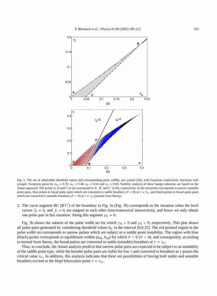
Fig. 3shows the set of admissible threshold values (Fig. 3a) and the corresponding pulse widths (Fig. 3b) for thesame connectivity functions as for the example pulses inFig. 1. The corners A, B and C inFig. 3acorrespond tothe corners A′, B′ and C′ in Fig. 3b, respectively, through the mapping process
(θe, θi ) → (a, b), fe(a, b) = θe, fi (a, b) = θi .
The following features are apparent:
1. The curve segment AB (A′B′) of the boundary inFig. 3a(Fig. 3b) corresponds a broad pulse pair coexistingwith a narrow pulse pair whereb → 0.
P. Blomquist et al. / Physica D 206 (2005) 180–212 193
Fig. 3. The set of admissible threshold values and corresponding pulse widths, see system(20), with Gaussian connectivity functions withsynaptic footprints given byσee = 0.35, σei = 0.48, σie = 0.60 andσii = 0.69. Stability analysis of these bumps solutions are based on theAmari approach. The points A, B and C in (a) correspond to A′, B′ and C′ in (b), respectively. In (b) red points corresponds to narrow unstablepulse pairs, blue points to broad pulse pairs which are converted to stable breathers (ϑ < 0) at τ = τcr, and black points to broad pulse pairswhich are converted to unstable breathers (ϑ > 0) atτ = τcr (normal form theory).
2. The curve segment BC (B′C′) of the boundary inFig. 3a(Fig. 3b) corresponds to the situation when the levelcurvesfe = θe andfi = θi are tangent to each other (non-transversal intersection), and hence we only obtainone pulse pair in this situation. Along this segmentγA = 0.
Fig. 3bshows the subsets of the pulse width set for whichγA > 0 andγA < 0, respectively. This plot showsall pulse pairs generated by considering threshold valuesθm in the interval [0,0.25]. The red pointed region in thepulse width set corresponds to narrow pulses which are subject to a saddle point instability. The region with blue(black) points corresponds to equilibrium widths (aeq, beq) for whichϑ < 0 (ϑ > 0), and consequently, accordingto normal form theory, the broad pulses are converted to stable (unstable) breathers atτ = τcr.
Thus, to conclude, the Amari analysis predicts that narrow pulse pairs are expected to be subject to an instabilityof the saddle point type, while the broader pulse pairs are stable for lowτ and converted to breathers asτ passes thecritical valueτcr. In addition, this analysis indicates that there are possibilities of having both stable and unstablebreathers excited at the Hopf bifurcation pointτ = τcr.
194 P. Blomquist et al. / Physica D 206 (2005) 180–212
5. Full stability analysis
In this section we study the stability of the pulse pairs with the full set of model equations(4) as a starting point,using a standard linearization procedure in a way identical to the one presented in Pinto and Ermentrout[13]. It isshown that one ends up with two eigenvalue equations of the same type as(39). These equations constitute the basisof the stability analysis. We compare the results of this approach with the simplified Amari analysis presented inthe previous section.
5.1. Linearized non-local equations
Let Ue andUi be a steady state pulse pair solution of(4), i.e.,
Ue = ωee∗ H(Ue − θe) − ωie ∗ H(Ui − θi ) (54a)
Ui = ωei ∗ H(Ue − θe) − ωii ∗ H(Ui − θi ). (54b)
We introduce the perturbed state
ue(x, t) = Ue(x) + χ(x, t), ui (x, t) = Ui (x) + ψ(x, t). (55)
Taylor expansion about the equilibrium state (Ue, Ui ) yields
H(Ue − θe + χ) = H(Ue − θe) + δ(Ue − θe)χ + . . . (56a)
H(Ui − θi + ψ) = H(Ui − θi ) + δ(Ui − θi )ψ + . . . . (56b)
Since, by assumption|χ| � |Ue − θe| and|ψ| � |Ui − θi | we retain only the two lowest order terms in the ex-pansion. Hereδ denotes the Dirac function. When inserting these approximations into(4)and taking the equilibriumcondition(54) into account, one deduces the linearized non-local evolution equations for the disturbances (χ,ψ)
χt = −χ + ωee∗ (δ(Ue − θe)χ) − ωie ∗ (δ(Ui − θi )ψ) (57a)
τψt = −ψ + ωei ∗ (δ(Ue − θe)χ) − ωii ∗ (δ(Ui − θi )ψ). (57b)
5.1.1. EigenvaluesWe then look for solutions of the form
χ(x, t) = eλtχ1(x) (58a)
ψ(x, t) = eλtψ1(x) (58b)
of the system(57) and get
(1 + λ)χ1(x) = ωee∗ (δ(Ue − θe)χ1) − ωie ∗ (δ(Ui − θi )ψ1) (59a)
(1 + λτ)ψ1(x) = ωei ∗ (δ(Ue − θe)χ1) − ωii ∗ (δ(Ui − θi )ψ1). (59b)
Hereλ plays the role of growth rate (Reλ > 0) or decay rate (Reλ < 0) of the disturbances (χ(x, t), ψ(x, t))imposed on the stationary pulse pair state (Ue(x), Ui (x)).
Again we exploit the identification of the equilibrium pulse pairs (Ue(x), Ui (x)) with pulse width coordinates(aeq, beq), through the equationsUm(x) = θm,0 < θm ≤ 1,m = e, i. We assume that the latter set of equationspossesses one and only one solution (aeq, beq) for which aeq, beq > 0. By making use of this assumption we can

P. Blomquist et al. / Physica D 206 (2005) 180–212 195
evaluate the convolution integralsωmn ∗ (δ(Um − θm)). The details in this evaluation is shown inAppendix B, andwe end up with
(1 + λ)χ1(x) = 1
|U ′e(aeq)| [ωee(x + aeq)χ1(−aeq) + ωee(x − aeq)χ1(aeq)]
− 1
|U ′i (beq)| [ωie(x + beq)ψ1(−beq) + ωie(x − beq)ψ1(beq)] (60a)
(1 + λτ)ψ1(x) = 1
|U ′e(aeq)| [ωei(x + aeq)χ1(−aeq) + ωei(x − aeq)χ1(aeq)]
− 1
|U ′i (beq)| [ωii (x + beq)ψ1(−beq) + ωii (x − beq)ψ1(beq)]. (60b)
The relations(60) imply the equivalence
χ1(aeq) = χ1(−aeq) = ψ1(beq) = ψ1(−beq) ≡ 0 ⇔ χ1(x) = ψ1(x) ≡ 0. (61)
Then, since we consider non-trivial spatial disturbances (χ1(x), ψ1(x)) the condition
X =
χ1(aeq)
χ1(−aeq)
ψ1(beq)
ψ1(−beq)
�= 0 (62)
has to be satisfied. The problem now consists of determining the eigenvalueλ for which(62)is fulfilled. We proceedas follows: By lettingx = ±aeq andx = ±beq in (60a) and (60b), respectively, we find
(1 + λ)χ1(aeq) = 1
|U ′e(aeq)| [ωee(0)χ1(aeq) + ωee(2aeq)χ1(−aeq)]
− 1
|U ′i (beq)| [ωie(aeq − beq)ψ1(b) + ωie(aeq + beq)ψ1(−beq)] (63a)
(1 + λ)χ1(−aeq) = 1
|U ′e(aeq)| [ωee(2aeq)χ1(aeq) + ωee(0)χ1(−aeq)]
− 1
|U ′i (beq)| [ωie(aeq + beq)ψ1(beq) + ωie(aeq − beq)ψ1(−beq)] (63b)
(1 + λτ)ψ1(beq) = 1
|U ′e(aeq)| [ωei(aeq − beq)χ1(aeq) + ωei(aeq + b)χ1(−aeq)]
− 1
|U ′i (beq)| [ωii (0)ψ1(beq) + ωii (2beq)ψ1(−beq)] (63c)
(1 + λτ)ψ1(−beq) = 1
|U ′e(aeq)| [ωei(aeq + beq)χ1(aeq) + ωei(aeq − beq)χ1(−aeq)]
− 1
|U ′i (beq)| [ωii (2beq)ψ1(beq) + ωii (0)ψ1(−beq)]. (63d)
196 P. Blomquist et al. / Physica D 206 (2005) 180–212
The system(63) is easily recognized as a linear homogeneous system of equations,
A · X = 0 (64)
where the matrixA is given by
A =
A1 − (1 + λ) B1 −C1 −D1
B1 A1 − (1 + λ) −D1 −C1
E1 F1 −G1 − (1 + λτ) −H1
F1 E1 −H1 −G1 − (1 + λτ)
, (65)
from which it follows thatλ is an eigenvalue of a 4× 4-matrix. For convenience, we have introduced the parametersA1, B1, C1,D1, E1, F1,G1 andH1 defined as
A1 = ωee(0)
|U ′e(aeq)| , B1 = ωee(2aeq)
|U ′e(aeq)| , (66a)
C1 = ωie(aeq − beq)
|U ′i (beq)| , D1 = ωie(aeq + beq)
|U ′i (beq)| , (66b)
E1 = ωei(aeq − beq)
|U ′e(aeq)| , F1 = ωei(aeq + beq)
|U ′e(aeq)| , (66c)
G1 = ωii (0)
|U ′i (beq)| , H1 = ωii (2beq)
|U ′i (beq)| . (66d)
Now, let
P =
1
2
1
20 0
0 01
2
1
21
2−1
20 0
0 01
2−1
2
(67)
and introduce the substitution
Y = P · X (68)
where
Y =
χe(aeq)
ψe(beq)
χo(aeq)
ψo(beq)
. (69)
P. Blomquist et al. / Physica D 206 (2005) 180–212 197
The subscripts e and o refer to the even and odd parts, respectively, of the functionsχ1 andψ1. The similaritytransformation(68)conveniently transformsA to the block-diagonal matrixPAP−1 given by
PAP−1 =
A1 + B1 − λ − 1 −C1 − D1 0 0
F1 + E1 −G1 − H1 − λτ − 1 0 0
0 0 A1 − B1 − λ − 1 −C1 + D1
0 0 −F1 + E1 −G1 + H1 − λτ − 1
. (70)
Then, we find that
det(PAP−1) = [τλ2 + (αL + βLτ)λ + γL] · [τλ2 + (α′L + β′
Lτ)λ + γ ′L] (71)
and hence the eigenvaluesλ are solutions to the quadratic equations
τλ2 + (αL − βLτ) λ + γL = 0 (72a)
τλ2 + (α′L − β′
Lτ)λ + γ ′L = 0. (72b)
Here
αL = 1 + G1 + H1, (73a)
βL = −1 + A1 + B1, (73b)
γL = 1 − (A1 + B1)(1 + G1 + H1) + G1 + H1 + (C1 + D1)(E1 + F1), (73c)
and
α′L = 1 + G1 − H1, (74a)
β′L = −1 + A1 − B1, (74b)
γ ′L = 1 − (A1 − B1)(1 + G1 − H1) + G1 − H1 + (C1 − D1)(E1 − F1). (74c)
Here the subscript ‘L’ is used in order to indicate that the stability analysis is based on the linearization procedureof the full model as opposed to the simplified Amari approach. In the following we will make use of the followingproperties:
1. From the definitions ofβL andβ′L, it follows thatβL ≥ β′
L.2. From the definition ofαL andα′
L, it follows thatαL > 0 and thatα′L ≤ αL. Moreover, sinceωii by assumption
is a decreasing function for positivex, α′L > 0. Thus we can conclude thatα′
L ≥ αL ≥ 0.3. One can prove thatγ ′
L ≡ 0. The proof of this is presented inAppendix C. This result reflects the translationinvariance of the pulse solutions, in the same way as observed in Pinto and Ermentrout[13].
6. Amari approach versus full stability analysis
In this section, we discuss the relationship between the Amari approach (Section4) and the full stability analysis(Section5). We first notice the structural equivalence between the eigenvalueproblems (39) and (72a), i.e., they canboth be written on the form
τλ2 + (αi − βiτ)λ + γi = 0, (i = A,L) (75)
198 P. Blomquist et al. / Physica D 206 (2005) 180–212
where the subscriptsi = A andi = L correspond to the Amari eigenvalue equation(39)and the quadratic equation(72a), respectively. InAppendix Cit is proved that
αA = αL, βA = βL, γA = γL, (76)
by means of some straightforward, but tedious algebraic computations. From now on we use the notation
α ≡ αA = αL, β ≡ βA = βL, γ ≡ γA = γL. (77)
Hence, the only difference between the two stability approaches consists of the presence of the additionaleigenvalue equation
τλ2 + (α′ − β′τ)λ = 0 (78)
in the full stability analysis, where we here and in the sequel for convenience employ the notationα′ ≡ α′L and
β′ ≡ β′L. The presence of equation(78) may affect the conclusions with respect to the stability/instability of the
pulse pairs.Here we will show that we can use the Amari analysis to predict stability versus instability of the pulse pairs,
with one notable exception.
1. Whenγ is negative we have a saddle point instability, irrespective of the properties of the roots of(78). Both thepulse widths and the synaptic footprints regulate the magnitude ofγ.
2. In the complementary regime, i.e., whenγ is positive, one has to separate the discussion into the followingsubcases:• β > 0 ≥ β′.
Even thoughβ according to the Amari analysis always is positive,β′ may be non-positive. In this case theequation(78)gives a negative value for the non-zero eigenvalue. But, sinceβ > 0, there is a Hopf bifurcationpoint at a criticalτ-value for(75), given byτ = τcr ≡ α
β. In this case the stability situation is governed by
(75).• β ≥ β′ > 0.
If β′ > 0, the following picture emerges: There are two different criticalτ-values,τcr andτ′cr, given as
τcr = α
βand τ′
cr = α′
β′ . (79)
Motivated by the results of the Amari approach, we will termτcr theHopf bifurcation point.
Forβ′, γ > 0, we can now infer that the Amari approach is applicable if
τcr ≤ τ′cr. (80)
One shows this as follows: Let us varyτ. Whenτ exceeds the Hopf bifurcation pointτcr, the real part of theeigenvalues of(75) changes from negative to positive, while the nontrivial eigenvalue of(78) remains negative.Hence the question about stability versus instability of the “bumps” can solely be based on(75).
In the complementary regime, i.e., when
τcr > τ′cr, (81)
the Amari approach predicts stability for the rangeτ′cr < τ < τcr, whereas the full linear stability analysis yields
instability in the same range of relative inhibition times. Hence the Amari approach gives correct stability predictionsexcept whenγ > 0, β ≥ β′ > 0 andτ′
cr < τ < τcr.In Fig. 4the applicability of Amari approach is demonstrated for the admissible set of threshold values when the
connectivity functions are as inFigs. 1–3. The following features are apparent: One can identify compact subsets in
P. Blomquist et al. / Physica D 206 (2005) 180–212 199
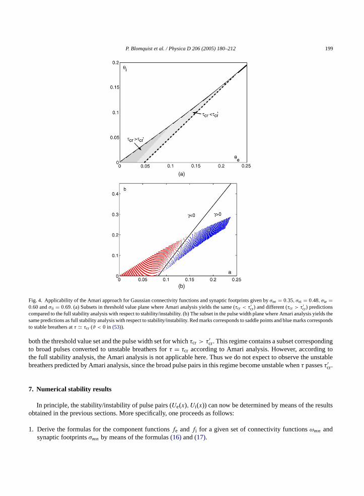
Fig. 4. Applicability of the Amari approach for Gaussian connectivity functions and synaptic footprints given byσee = 0.35, σei = 0.48, σie =0.60 andσii = 0.69. (a) Subsets in threshold value plane where Amari analysis yields the same (τcr < τ′
cr) and different (τcr > τ′cr) predictions
compared to the full stability analysis with respect to stability/instability. (b) The subset in the pulse width plane where Amari analysis yields thesame predictions as full stability analysis with respect to stability/instability. Red marks corresponds to saddle points and blue marks correspondsto stable breathers atτ � τcr (ϑ < 0 in (53)).
both the threshold value set and the pulse width set for whichτcr > τ′cr. This regime contains a subset corresponding
to broad pulses converted to unstable breathers forτ = τcr according to Amari analysis. However, according tothe full stability analysis, the Amari analysis is not applicable here. Thus we do not expect to observe the unstablebreathers predicted by Amari analysis, since the broad pulse pairs in this regime become unstable whenτ passesτ′
cr.
7. Numerical stability results
In principle, the stability/instability of pulse pairs (Ue(x), Ui (x)) can now be determined by means of the resultsobtained in the previous sections. More specifically, one proceeds as follows:
1. Derive the formulas for the component functionsfe andfi for a given set of connectivity functionsωmn andsynaptic footprintsσmn by means of the formulas(16)and(17).
200 P. Blomquist et al. / Physica D 206 (2005) 180–212
2. Determine the pulse width coordinates (aeq, beq) of the pulse pairs (Ue(x), Ui (x)) by solving the system(15) fora given set of admissible threshold values (θe, θi ).
3. Compute the parametersα, β, γ, α′ andβ′ by means of the expressions(66a), (66b), (66c), (66d), (73a), (73b),(73c), (74a) and (74b).
4. Use the classification scheme described in Section6to infer conclusions about stability/instability of the “bumps”-solutions.
In general, due to the complicated mathematical structure involved it is difficult to extract generic conclusionswith respect to the stability/instability of the “bumps”. In most cases one has to rely on numerical computations.
We follow the four step procedure described above for the example shown inFig. 1:
1. The synaptic footprints are chosen to be
σee = 0.35, σei = 0.48, σie = 0.60, σii = 0.69 (82)
and all the connectivity functions are assumed to be Gaussians(6) and (7).2. The threshold values for firing are chosen as
θe = 0.12, θi = 0.08. (83)
This choice of threshold values yields two solutions of the system(15), which indeed correspond to the situ-ation with two separate pulse pairs, as explained in Section3. The pulse width coordinates are (a
(1)eq, b
(1)eq) =
(0.066,0.045) and (a(2)eq, b
(2)eq) = (0.179,0.183). For convenience and in analogy with[13], we term the pulse
pair corresponding to (a(1)eq, b
(1)eq) = (0.066,0.045) as thenarrow pulse pair, while (a(2)
eq, b(2)eq) = (0.179,0.183)
is referred to as thebroad pulse pair.3. The parametersα, β, γ, α′ andβ′ have been computed separately for each pulse pair. We find the parameter set
α = 36.81, β = 15.36, γ = −58.03, α′ = 1.31, β′ = 0.17 (84)
for the narrow pulse pair, while we get
α = 5.63, β = 1.86, γ = 1.97, α′ = 1.65, β′ = 0.38 (85)
for the broad pulse pair. Hence, we can conclude that the narrow pulse pair is unstable in the saddle-point sensesinceγ < 0. The broad pulse pair is stable for small and moderate relative inhibition times. When the relativeinhibition time exceeds a criticalτ value, the broad pulses become unstable. First, it should be noticed that bothβ andβ′ are positive, so that we are in the regime where there are two critical relative inhibition times,τcr = α
β,
andτ′cr = α′
β′ . Secondly, since
τcr = 3.03, τ′cr = 4.36, (86)
we haveτcr < τ′cr, and hence the change from stability to instability occurs as the relative inhibition time exceeds
τcr. Notice that sinceτcr < τ′cr Amari’s stability analysis can be used to reach the conclusion regarding the
stability properties of the broad pulse pair.
We have carried out numerical simulations of the full system of equations(4) with the stationary pulse pair(Ue(x), Ui (x)) as initial condition, using the set of input parameters listed above. These simulations are based ona split step approach where the time evolution is resolved by means of fourth order Runge–Kutta in time. At eachtime step,tj, we numerically detect the pulse widths of each pulse by means of the constraint equation
um(a(tj), tj) = θm for m = e, i. (87)
P. Blomquist et al. / Physica D 206 (2005) 180–212 201
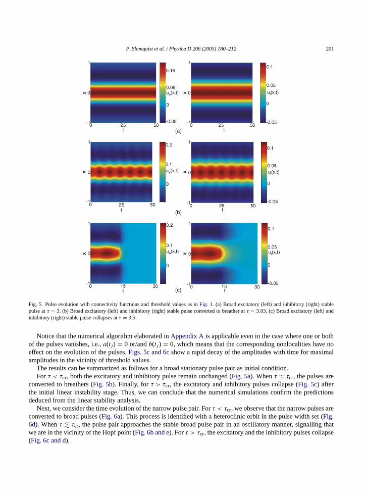
Fig. 5. Pulse evolution with connectivity functions and threshold values as inFig. 1. (a) Broad excitatory (left) and inhibitory (right) stablepulse atτ = 3. (b) Broad excitatory (left) and inhibitory (right) stable pulse converted to breather atτ = 3.03, (c) Broad excitatory (left) andinhibitory (right) stable pulse collapses atτ = 3.5.
Notice that the numerical algorithm elaborated inAppendix Ais applicable even in the case where one or bothof the pulses vanishes, i.e.,a(tj) = 0 or/andb(tj) = 0, which means that the corresponding nonlocalities have noeffect on the evolution of the pulses.Figs. 5c and 6cshow a rapid decay of the amplitudes with time for maximalamplitudes in the vicinity of threshold values.
The results can be summarized as follows for a broad stationary pulse pair as initial condition.For τ < τcr, both the excitatory and inhibitory pulse remain unchanged (Fig. 5a). Whenτ � τcr, the pulses are
converted to breathers (Fig. 5b). Finally, for τ > τcr, the excitatory and inhibitory pulses collapse (Fig. 5c) afterthe initial linear instability stage. Thus, we can conclude that the numerical simulations confirm the predictionsdeduced from the linear stability analysis.
Next, we consider the time evolution of the narrow pulse pair. Forτ < τcr, we observe that the narrow pulses areconverted to broad pulses (Fig. 6a). This process is identified with a heteroclinic orbit in the pulse width set (Fig.6d). Whenτ � τcr, the pulse pair approaches the stable broad pulse pair in an oscillatory manner, signalling thatwe are in the vicinity of the Hopf point (Fig. 6b and e). Forτ > τcr, the excitatory and the inhibitory pulses collapse(Fig. 6c and d).

202 P. Blomquist et al. / Physica D 206 (2005) 180–212
Fig. 6. Evolution of unstable narrow pulse pairs with connectivity functions and threshold values as inFig. 1. (a) Narrow excitatory (left) andinhibitory (right) pulse convert to broad inhibitory pulse atτ = 2.5. (b) Narrow excitatory (left) and inhibitory (right) pulse convert to stableexcitatory and inhibitory breathers atτ = 3.0. (c) Narrow excitatory (left) and inhibitory (right) pulse collapse atτ = 3.5. (d) Heteroclinic orbitin the pulse width plane forτ = 2.5 andτ = 3.5. Forτ = 3.5, we observe pulse pair collapse in the pulse width set. (e) Same as (d) forτ = 3.0.The pulse width of the narrow pulse pair approaches the pulse width of the broad pulse pair in an oscillatory manner, signalling that we are inthe vicinity of the Hopf point atτ = 3.0.
P. Blomquist et al. / Physica D 206 (2005) 180–212 203
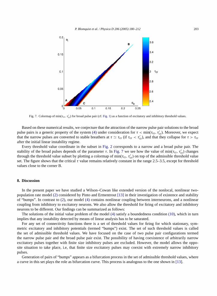
Fig. 7. Colormap of min(τcr, τ′cr) for broad pulse pair (cf.Fig. 1) as a function of excitatory and inhibitory threshold values.
Based on these numerical results, we conjecture that the attraction of the narrow pulse pair solutions to the broadpulse pairs is a generic property of the system(4) under consideration forτ < min(τcr, τ
′cr). Moreover, we expect
that the narrow pulses are converted to stable breathers atτ � τcr (if τcr < τ′cr), and that they collapse forτ > τcr
after the initial linear instability regime.Every threshold value coordinate in the subset inFig. 2 corresponds to a narrow and a broad pulse pair. The
stability of the broad pulses depends of the parameterτ. In Fig. 7 we see how the value of min(τcr, τ′cr) changes
through the threshold value subset by plotting a colormap of min(τcr, τ′cr) on top of the admissible threshold value
set. The figure shows that the criticalτ value remains relatively constant in the range 2.5–3.5, except for thresholdvalues close to the corner B.
8. Discussion
In the present paper we have studied a Wilson–Cowan like extended version of the nonlocal, nonlinear two-population rate model(2) considered by Pinto and Ermentrout[13] in their investigation of existence and stabilityof “bumps”. In contrast to(2), our model(4) contains nonlinear coupling between interneurons, and a nonlinearcoupling from inhibitory to excitatory neurons. We also allow the threshold for firing of excitatory and inhibitoryneurons to be different. Our findings can be summarized as follows:
The solutions of the initial value problem of the model(4) satisfy a boundedness condition(10), which in turnimplies that any instability detected by means of linear analysis has to be saturated.
For any set of connectivity functions there is a set of threshold values for firing for which stationary, sym-metric excitatory and inhibitory potentials (termed “bumps”) exist. The set of such threshold values is calledthe set of admissible threshold values. We have focused on the case of two pulse pair configurations termedthe narrow pulse pair and the broad pulse pair exist. The possibility of having coexistence of arbitrarily narrowexcitatory pulses together with finite size inhibitory pulses are excluded. However, the model allows the oppo-site situation to take place, i.e, that finite size excitatory pulses may coexist with extremely narrow inhibitorypulses.
Generation of pairs of “bumps” appears as a bifurcation process in the set of admissible threshold values, wherea curve in this set plays the role as bifurcation curve. This process is analogous to the one shown in[13].
204 P. Blomquist et al. / Physica D 206 (2005) 180–212
The stability of the pair of “bumps” is studied by means of Amari’s simplified approach, i.e, by investigatingthe stability of the pulse widths of the pulses. This stability analysis is based on a quadratic eigenvalue equa-tion where the relative inhibition time plays the role as control parameter. The narrow pulse pairs are genericallyunstable of the saddle point type, while the broad pulse pairs are shown to be stable for small and moderatevalues of the relative inhibition time. Regimes producing change from stability to instability through a Hopf bi-furcation are identified. Moreover, the stability of the limit cycle formed at the bifurcation point is addressedusing the theory of normal forms for 2D systems. Numerical investigation of the outcome of our Amari-typeanalysis confirm that both stable and unstable breathers can be excited at the Hopf bifurcation point (cf.Fig.3b).
The stability analysis based on Amari’s approach is parallelled by a rigorous stability analysis of the “bumps”using the full set of equations(4) and the “bumps” as a starting point. It is readily shown that the eigenvalue problemfactorizes into a product of two quadratic polynomials of which one is identified with the Amari eigenvalue problem.A scheme for determining the stability is then devised, and it is shown that the Amari approach and the full analysisyield the same predictions, with one notable exception.
The stability of “bumps” is investigated numerically by means of a split step scheme where the time evolution isresolved by means of a fourth order Runge–Kutta method. This investigation reveals that narrow “bumps” seem to beunstable for all relative inhibition times, while broad “bumps” are stable for small and moderate relative inhibitiontimes. However, when the relative inhibition time exceeds a certain threshold, the “bumps” become unstable. Onenotices that this feature also appears in[13]. In some of our numerical investigations this threshold is lower thanthe threshold for stability predicted by the Amari approach.
We also observe stable breathers numerically asτ passes the Hopf bifurcation pointτcr predicted by the Amariapproach. However, the unstable breathers are not expected to be seen at this point, since full stability analysispredicts that the broad pairs corresponding to these breathers have become unstable for relative inhibition timesbelow the Hopf bifurcation point.
The observation of stable breathers in our model contrasts the numerical observations of the model(2) reportedin [13] where only unstable periodic solutions were seen, suggesting a subcritical Hopf bifurcation. A similarconclusion was reached in[27]. Stable breathers could be generated in a similar model, however, by inclusion oflocalized inputs breaking the spatial homogeneity[20]. Interestingly, Coombes and Owen[26] recently observedstable breathing solutions in a homogeneous model with a Mexican-hat like connectivity when a dynamic firingthreshold was incorporated. This could hint that our observation of stable breathers is related to the incorporationof two independent firing thresholds in the present model(4). However, we have observed stable breathers in ourmodel even whenθe = θi (for example,θe = θi = 0.2, with the same synaptic footprints as inFig. 1). Notice thatthis situation is outside the generic two pulse pair regime displayed inFig. 2. One can show that this choice ofthreshold values (θe, θi ) gives rise to a single pulse pair solution. However, the same stability analysis as elaboratedin this paper is applicable in this case.
In our numerical example in Section7 we foundτcr to be 3.03. Thus stable bumps were found to exist even withan inhibitory time constant a factor three larger than the excitatory time constant. This contrasts the analogous resultfrom the analysis of the model considered by Pinto and Ermentrout[13] whereτcr was found to be significantlysmaller than one. Thus, our model results do not support the claim that slow excitation mediated by say NMDA-receptors is needed to allow stable bumps[9].
Hansel and Mato[30] studied stability of persistent states in large networks of spiking excitatory and inhibitoryneurons of the quadratic integrate-and-fire type. In their two-population model without any spatial structure theyfound that so called asynchronous persistent states could be obtained more easily when inhibitory–inhibitory in-teractions were included. We have not done a systematic study of the parameter-dependence of bump stability inour rate model. However, since rate models are expected to be able to describe asynchrononous states, Hansel andMato’s observation suggests that the larger range ofτ allowing stable bumps in our model may stem from theinclusion of the inhibitory–inhibitory interaction, i.e.,wii (x) �= 0. This interaction was absent in the model studiedby Pinto and Ermentrout[13].
P. Blomquist et al. / Physica D 206 (2005) 180–212 205
Acknowledgements
The authors will like to thank Wieslaw Krolikowski, Yuri Kivshar, Andrey Miroshnischenko and Hans EkkehardPlesser for many fruitful and stimulating discussions during the preparation phase of the present paper. Most ofthe figures in the present paper is generated by means of the supercomputer Caspar at the Norwegian University ofLife Sciences. P. Blomquist was supported by the Research Council of Norway under the grant No. 160011/V30.J. Wyller acknowledges support from Centre for Integrative Genetics and the Research Council of Norway underthe grant No. 153405/432. The present work was completed in 2003/04 when J. Wyller was a Visiting Fellowat Nonlinear Physics Centre and Laser Physics Centre, Australian National University. We will like to thank thereviewers for constructive remarks.
Appendix A. Runge–Kutta split step method
Here we design a numerical code for the initial value problem of system(4) with all the firing rate functionsapproximated with the Heaviside step function. The code is based on a so-calledsplit-step approach. The startingpoint is to study the time evolution on a time interval referred to asthe time stepping length. The non-localitieswhich contain the nonlinear effects are treated as constants on this particular interval. The time-evolution whichis described by a set of ordinary differential equations, can be resolved by means of a finite difference scheme forsuch equations. Here we will employ the fourth order Runge–Kutta method in order to solve this problem.
We discretise the time interval, i.e., introduce the sequence{tj}Nj=0 wheret0 ≡ 0 and the time stepping lengthCtj ≡ tj+1 − tj. LetXj andF (Xj) be the 2D vector fields defined as
Xj =(ue(x, tj)
ui (x, tj)
), F (Xj) =
(fj
gj
)
where the componentsfj andgj are given as
fj = −ue(x, tj) + �j (A.1a)
gj = −1
τui (x, tj) + 1
τDj (A.1b)
with
�j ≡ 0ee(a(tj) + x) + 0ee(a(tj) − x) − 0ie(b(tj) + x) − 0ie(b(tj) − x) (A.2a)
Dj ≡ 0ei(a(tj) + x) + 0ei(a(tj) − x) − 0ii (b(tj) + x) − 0ii (b(tj) − x) (A.2b)
and
0mn(x) ≡∫ x
0ωmn(y) dy =
∫ x/σmn
0�mn(y) dy (A.3)
where we have taken into account the generic form of the connectivity functionsωmn(x) = σ−1mn�mn(ξmn),
ξmn = x/σmn.The width coordinatesa(tj) andb(tj) appearing in the expressions�j andDj satisfy the constraints
ue(a(tj), tj) = θe, ui (b(tj), tj) = θi . (A.4)
The fourth order Runge–Kutta code can now be formulated as follows:
206 P. Blomquist et al. / Physica D 206 (2005) 180–212
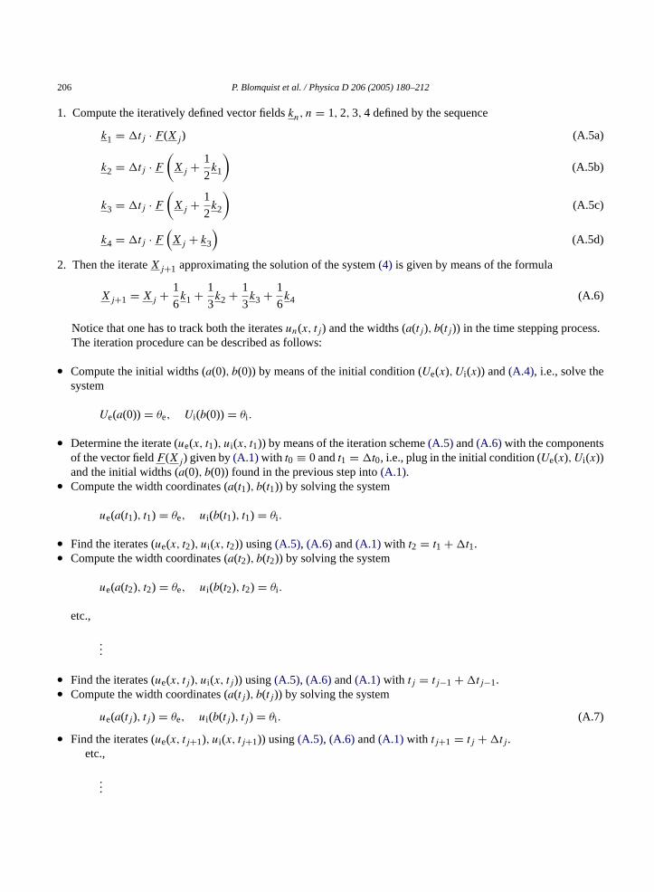
1. Compute the iteratively defined vector fieldskn, n = 1,2,3,4 defined by the sequence
k1 = Ctj · F (Xj) (A.5a)
k2 = Ctj · F(Xj + 1
2k1
)(A.5b)
k3 = Ctj · F(Xj + 1
2k2
)(A.5c)
k4 = Ctj · F(Xj + k3
)(A.5d)
2. Then the iterateXj+1 approximating the solution of the system(4) is given by means of the formula
Xj+1 = Xj + 1
6k1 + 1
3k2 + 1
3k3 + 1
6k4 (A.6)
Notice that one has to track both the iteratesun(x, tj) and the widths (a(tj), b(tj)) in the time stepping process.The iteration procedure can be described as follows:
• Compute the initial widths (a(0), b(0)) by means of the initial condition (Ue(x), Ui (x)) and(A.4), i.e., solve thesystem
Ue(a(0)) = θe, Ui (b(0)) = θi .
• Determine the iterate (ue(x, t1), ui (x, t1)) by means of the iteration scheme(A.5) and(A.6) with the componentsof the vector fieldF (Xj) given by(A.1) with t0 ≡ 0 andt1 = Ct0, i.e., plug in the initial condition (Ue(x), Ui (x))and the initial widths (a(0), b(0)) found in the previous step into(A.1).
• Compute the width coordinates (a(t1), b(t1)) by solving the system
ue(a(t1), t1) = θe, ui (b(t1), t1) = θi .
• Find the iterates (ue(x, t2), ui (x, t2)) using(A.5), (A.6) and(A.1) with t2 = t1 + Ct1.• Compute the width coordinates (a(t2), b(t2)) by solving the system
ue(a(t2), t2) = θe, ui (b(t2), t2) = θi .
etc.,
...
• Find the iterates (ue(x, tj), ui (x, tj)) using(A.5), (A.6) and(A.1) with tj = tj−1 + Ctj−1.• Compute the width coordinates (a(tj), b(tj)) by solving the system
ue(a(tj), tj) = θe, ui (b(tj), tj) = θi . (A.7)
• Find the iterates (ue(x, tj+1), ui (x, tj+1)) using(A.5), (A.6) and(A.1) with tj+1 = tj + Ctj.etc.,
...
P. Blomquist et al. / Physica D 206 (2005) 180–212 207
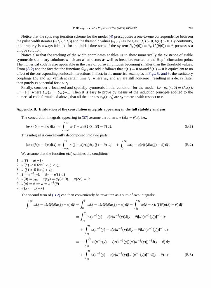
Notice that the split step iteration scheme for the model(4) presupposes a one-to-one correspondence betweenthe pulse width iterates (a(tj), b(tj)) and the threshold values (θe, θi ) as long asa(tj) > 0, b(tj) > 0. By continuity,this property is always fulfilled for the initial time steps if the systemUe(a(0)) = θe, Ui (b(0)) = θi possesses aunique solution.
Notice also that the tracking of the width coordinates enables us to show numerically the existence of stablesymmetric stationary solutions which act as attractors as well as breathers excited at the Hopf bifurcation point.The numerical code is also applicable in the case of pulse amplitudes becoming smaller than the threshold values.From(A.2) and the fact that the functions0mn are odd it follows thata(tj) = 0 or/andb(tj) = 0 is equivalent to noeffect of the corresponding nonlocal interactions. In fact, in the numerical examples inFigs. 5c and 6cthe excitatorycouplings0ee and0ei vanish at certain timet∗ (where0ie and0ii are still non-zero), resulting in a decay fasterthan purely exponential fort > t∗.
Finally, consider a localized and spatially symmetric initial condition for the model, i.e.,um(x,0) = Um(x);m = e, i, whereUm(x) = Um(−x). Then it is easy to prove by means of the induction principle applied to thenumerical code formulated above, that all the iteratesum(x, tj) are symmetric with respect tox.
Appendix B. Evaluation of the convolution integrals appearing in the full stability analysis
The convolution integrals appearing in(57)assume the formω ∗ (δ(u − θ)z), i.e.,
[ω ∗ (δ(u − θ)z)](x) =∫ ∞
−∞ω(ξ − x)z(ξ)δ(u(ξ) − θ) dξ. (B.1)
This integral is conveniently decomposed into two parts:
[ω ∗ (δ(u − θ)z)](x) =∫ 0
−∞ω(ξ − x)z(ξ)δ(u(ξ) − θ) dξ +
∫ ∞
0ω(ξ − x)z(ξ)δ(u(ξ) − θ) dξ. (B.2)
We assume that the functionu(ξ) satisfies the conditions
1. u(ξ) = u(−ξ)2. u′(ξ) < 0 for 0< ξ < ξ13. u′(ξ) > 0 for ξ > ξ14. ξ = u−1(y), dy = u′(ξ)dξ5. u(0) = y0, u(ξ1) = y1(< 0), u(∞) = 06. u(a) = θ ⇒ a = u−1(θ)7. ω(x) = ω(−x)
The second term of(B.2) can then conveniently be rewritten as a sum of two integrals:∫ ∞
0ω(ξ − x)z(ξ)δ(u(ξ) − θ) dξ =
∫ ξ1
0ω(ξ − x)z(ξ)δ(u(ξ) − θ) dξ +
∫ ∞
ξ1
ω(ξ − x)z(ξ)δ(u(ξ) − θ) dξ
=∫ y1
y0
ω(u−1(y) − x)z(u−1(y))δ(y − θ)[u′(u−1(y))]−1 dy
+∫ 0
y1
ω(u−1(y) − x)z(u−1(y))δ(y − θ)[u′(u−1(y))]−1 dy
= −∫ y0
y1
ω(u−1(y) − x)z(u−1(y))[u′(u−1(y))]−1δ(y − θ) dy
+∫ 0
y1
ω(u−1(y) − x)z(u−1(y))[u′(u−1(y))]−1δ(y − θ) dy (B.3)
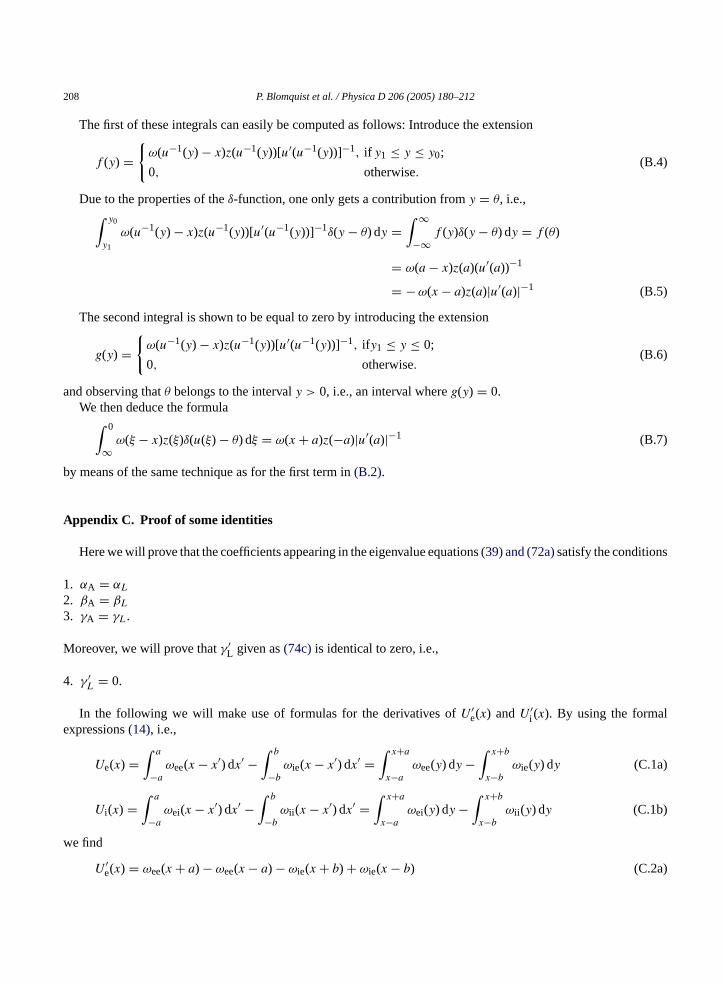
208 P. Blomquist et al. / Physica D 206 (2005) 180–212
The first of these integrals can easily be computed as follows: Introduce the extension
f (y) ={ω(u−1(y) − x)z(u−1(y))[u′(u−1(y))]−1, if y1 ≤ y ≤ y0;
0, otherwise.(B.4)
Due to the properties of theδ-function, one only gets a contribution fromy = θ, i.e.,∫ y0
y1
ω(u−1(y) − x)z(u−1(y))[u′(u−1(y))]−1δ(y − θ) dy =∫ ∞
−∞f (y)δ(y − θ) dy = f (θ)
= ω(a − x)z(a)(u′(a))−1
= −ω(x − a)z(a)|u′(a)|−1 (B.5)
The second integral is shown to be equal to zero by introducing the extension
g(y) ={ω(u−1(y) − x)z(u−1(y))[u′(u−1(y))]−1, ify1 ≤ y ≤ 0;
0, otherwise.(B.6)
and observing thatθ belongs to the intervaly > 0, i.e., an interval whereg(y) = 0.We then deduce the formula∫ 0
∞ω(ξ − x)z(ξ)δ(u(ξ) − θ) dξ = ω(x + a)z(−a)|u′(a)|−1 (B.7)
by means of the same technique as for the first term in(B.2).
Appendix C. Proof of some identities
Here we will prove that the coefficients appearing in the eigenvalue equations(39) and (72a)satisfy the conditions
1. αA = αL
2. βA = βL
3. γA = γL.
Moreover, we will prove thatγ ′L given as(74c)is identical to zero, i.e.,
4. γ ′L = 0.
In the following we will make use of formulas for the derivatives ofU ′e(x) andU ′
i (x). By using the formalexpressions(14), i.e.,
Ue(x) =∫ a
−a
ωee(x − x′) dx′ −∫ b
−b
ωie(x − x′) dx′ =∫ x+a
x−a
ωee(y) dy −∫ x+b
x−b
ωie(y) dy (C.1a)
Ui (x) =∫ a
−a
ωei(x − x′) dx′ −∫ b
−b
ωii (x − x′) dx′ =∫ x+a
x−a
ωei(y) dy −∫ x+b
x−b
ωii (y) dy (C.1b)
we find
U ′e(x) = ωee(x + a) − ωee(x − a) − ωie(x + b) + ωie(x − b) (C.2a)
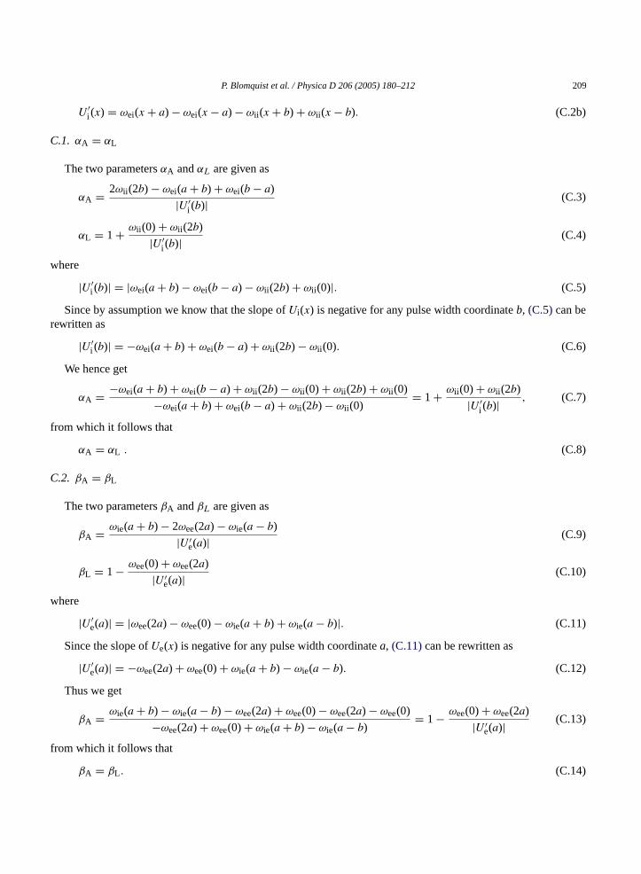
P. Blomquist et al. / Physica D 206 (2005) 180–212 209
U ′i (x) = ωei(x + a) − ωei(x − a) − ωii (x + b) + ωii (x − b). (C.2b)
C.1. αA = αL
The two parametersαA andαL are given as
αA = 2ωii (2b) − ωei(a + b) + ωei(b − a)
|U ′i (b)| (C.3)
αL = 1 + ωii (0) + ωii (2b)
|U ′i (b)| (C.4)
where
|U ′i (b)| = |ωei(a + b) − ωei(b − a) − ωii (2b) + ωii (0)|. (C.5)
Since by assumption we know that the slope ofUi (x) is negative for any pulse width coordinateb, (C.5)can berewritten as
|U ′i (b)| = −ωei(a + b) + ωei(b − a) + ωii (2b) − ωii (0). (C.6)
We hence get
αA = −ωei(a + b) + ωei(b − a) + ωii (2b) − ωii (0) + ωii (2b) + ωii (0)
−ωei(a + b) + ωei(b − a) + ωii (2b) − ωii (0)= 1 + ωii (0) + ωii (2b)
|U ′i (b)| , (C.7)
from which it follows that
αA = αL . (C.8)
C.2. βA = βL
The two parametersβA andβL are given as
βA = ωie(a + b) − 2ωee(2a) − ωie(a − b)
|U ′e(a)| (C.9)
βL = 1 − ωee(0) + ωee(2a)
|U ′e(a)| (C.10)
where
|U ′e(a)| = |ωee(2a) − ωee(0) − ωie(a + b) + ωie(a − b)|. (C.11)
Since the slope ofUe(x) is negative for any pulse width coordinatea, (C.11)can be rewritten as
|U ′e(a)| = −ωee(2a) + ωee(0) + ωie(a + b) − ωie(a − b). (C.12)
Thus we get
βA = ωie(a + b) − ωie(a − b) − ωee(2a) + ωee(0) − ωee(2a) − ωee(0)
−ωee(2a) + ωee(0) + ωie(a + b) − ωie(a − b)= 1 − ωee(0) + ωee(2a)
|U ′e(a)| (C.13)
from which it follows that
βA = βL . (C.14)
210 P. Blomquist et al. / Physica D 206 (2005) 180–212
C.3. γA = γL
The two parametersγA andγL depend on the connectivity functions in a complicated way. For convenience, weintroduce the parametersA2, B2, C2,D2, E2 andF2 defined by
A2 = ωee(2a)
|U ′e(a)| , B2 = ωie(a + b)
|U ′e(a)| , C2 = ωie(a − b)
|U ′e(a)| (C.15)
D2 = ωei(a + b)
|U ′i (b)| , E2 = ωei(b − a)
|U ′i (b)| , F2 = ωii (2b)
|U ′i (b)| . (C.16)
γA andγL can then be expressed as
γA = 2A2D2 − 2A2E2 − 4A2F2 + 2B2E2 + 2B2F2 + 2C2D2 − 2C2F2 (C.17)
γL = αLβL +(ωie(a − b)
|U ′i (b)| + ωie(a + b)
|U ′i (b)|
)(ωei(a − b)
|U ′e(a)| + ωei(a + b)
|U ′e(a)|
). (C.18)
Moreover, the latter expression forγL can easily be expressed in terms ofA2, B2, C2,D2, E2 andF2 as
γL = (2F2 − D2 + E2)(B2 − 2A2 − C2) + C2E2 + C2D2 + B2E2 + B2D2
= 2A2D2 − 2A2E2 − 4A2F2 + 2B2E2 + 2B2F2 + 2C2D2 − 2C2F2 , (C.19)
Hence
γA = γL . (C.20)
C.4. γ ′L = 0
γ ′L is given as
γ ′L = 1 −
(ωee(0)
|U ′e(a)| − ωee(2a)
|U ′e(a)|
)(1 + ωii (0)
|U ′i (b)| − ωii (2b)
|U ′i (b)|
)+(
ωii (0)
|U ′i (b)| − ωii (2b)
|U ′i (b)|
)
+(ωie(a − b)
|U ′i (b)| − ωie(a + b)
|U ′i (b)|
)(ωei(a − b)
|U ′e(a)| − ωei(a + b)
|U ′e(a)|
)(C.21)
which can be rewritten on the convenient form
γ ′L = 1 + A3 − B3
|A3 + B3 + C3| + D3 + E3 (C.22)
when introducing
A3 = ωee(0)ωii (2b) − ωee(0)ωii (0) − ωee(2a)ωii (2b) + ωee(2a)ωii (0) (C.23)
B3 = ωie(a − b)ωei(a + b) − ωie(a − b)ωei(a − b) + ωie(a + b)ωei(a − b) − ωei(a + b)ωie(a + b) (C.24)
C3 = ωee(2a)ωei(a + b) − ωee(2a)ωei(a − b) − ωee(0)ωei(a + b) + ωee(0)ωei(a − b)
+ωie(a + b)ωii (2b) − ωie(a + b)ωii (0) − ωie(a − b)ωii (2b) + ωie(a − b)ωii (0) (C.25)
D3 = ωee(2a) − ωee(0)
|ωee(2a) − ωee(0) − ωie(a + b) + ωie(a − b)| (C.26)
P. Blomquist et al. / Physica D 206 (2005) 180–212 211
E3 = ωii (0) − ωii (2b)
|ωii (0) − ωii (2b) + ωei(a + b)ωei(a − b)| . (C.27)
One can now prove that|A3 + B3 + C3| = |U ′e(a)U ′
i (b)|. Then, by some tedious algebraic manipulations we canshow that
A3 − B3
|A3 + B3 + C3| + D3 + E3 = −1 (C.28)
which finally yieldsγ ′L = 0 for everya andb, and independent of the synaptic footprints,σmn.
References
[1] X.-J. Wang, Synaptic reverbation underlying mnemonic persistent activity, Trends Neurosci. 24 (2001) 455–463.[2] H.R. Wilson, J.D. Cowan, A mathematical theory of the functional dynamics of cortical and thalamic nervous tissue, Kybern 13 (1973)
55–80.[3] S. Amari, Dynamics of pattern formation in lateral-inhibition type neural fields, Bio. Cybernet. 27 (1977) 77–87.[4] K. Kishimoto, S. Amari, Existence and stability of local excitations in homogeneous neural fields, J. Math. Biol. 7 (1979) 303–318.[5] D.J. Amit, N. Brunel, Model of global spontaneous activity and local structured activity during delay periods in the cerebral cortex, Cereb.
Cort. 7 (1997) 237–252.[6] M. Camperi, X.-J. Wang, A model of visuospatial working memory in prefrontal cortex: Recurrent network and cellular bistability, J.
Comp. Neurosci. 5 (1998) 383–405.[7] G.B. Ermentrout, Neural networks as spatio-temporal pattern-forming systems, Rep. Prog. Phys. 61 (1998) 353–430.[8] D. Hansel, H. Sompolinsky, Modeling feature selectivity in local cortical circuits, in: C. Koch, I. Segev (Eds.), Methods in Neuronal
Modeling: From Ions To Networks, second ed., MIT Press, Cambridge, MA, 1998, pp. 499–567.[9] A. Compte, N. Brunel, P.S. Goldman-Rakic, X.-J. Wang, Synaptic mechanisms and network dynamics underlying spatial working memory
in a cortical network model, Cereb. Cort. 10 (2000) 1627–1647.[10] B.S. Gutkin, G.B. Ermentrout, J. O’Sullivan, Layer 3 patchy recurrent excitatory connections mey determine the spatial organization of
sustained activity in the primate prefrontal cortex, Neurocom 32–33 (2000) 391–400.[11] B.S. Gutkin, C.R. Laing, C.L. Colby, C.C. Chow, G.B. Ermentrout, Turning on and off with excitation: the role of spike-timing asynchrony
and synchromy in sustained neural activity, J. Comp. Neurosci. 11 (2001) 121–134.[12] C.R. Laing, C.C. Chow, Stationary bumps in networks, Neural Comp. 13 (2001) 1473–1494.[13] D.J. Pinto, G.B. Ermentrout, Spatially structured activity in synaptically coupled neuronal networks: II. Lateral inhibition and standing
pulses, SIAM J. Appl. Math. 62 (1) (2001) 226–243.[14] J.E. Rubin, D. Terman, C. Chow, Localized bumps of activity sustained by inhibition in a two-layer thalamic network, J. Comp. Neurosci.
10 (2001) 313–331.[15] C.R. Laing, W.C. Troy, B. Gutkin, G.B. Ermentrout, Multiple bumps in a neuronal network model of working memory, SIAM J. Appl.
Math. 63 (2002) 62–97.[16] S. Coombes, G.J. Lord, M.R. Owen, Waves and bumps in neuronal networks with axon-dendritic synaptic interactions, Physica D 178
(2003) 219–241.[17] J. Drover, G.B. Ermentrout, Nonlinear coupling near a degenerate Hopf (Bautin) bifurcation, SIAM J. Appl. Math. 63 (2003) 1627–1647.[18] C.R. Laing, W.C. Troy, Two-bump solutions af Amari-type models of neuronal pattern formation, Physica D 178 (2003) 190–218.[19] S. Coombes, M.R. Owen, Evans functions for integral neural field equations with Heaviside firing rate functions, SIAM J. Appl. Dyn. Sys.
34 (2004) 574–600.[20] S.E. Folias, P.C. Bressloff, Breathing pulses in an excitatory neural network, SIAM J. Appl. Dyn. Sys. 3 (2004) 378–407.[21] J.E. Rubin, W.C. Troy, Sustained spatial patterns of activity in neuronal populations without recurrent excitation, SIAM J. Appl. Math. 64
(2004) 1609–1635.[22] J.E. Rubin, A. Bose, Localized activity patterns in excitatory neuronal networks, Network Comp. Neur. Syst. 15 (2004) 133–158.[23] Y. Guo, C.C. Chow, Existence and stability of standing pulses in neural networks: I. Existence, SIAM J. Appl. Dyn. Sys. 4 (2005) 217–
248.[24] Y. Guo, C.C. Chow, Existence and stability of standing pulses in neural networks: II. Stability, SIAM J. Appl. Dyn. Sys. 4 (2005) 249–
281.[25] D.J. Pinto, R.K. Jackson, C.E. Wayne, Existence and stability of traveling pulses in a continuous neuronal network, SIAM J. Appl. Dyn.
Sys., in press.

212 P. Blomquist et al. / Physica D 206 (2005) 180–212
[26] S. Coombes, M.R. Owen, Bumps, breathers, and waves in a neural network with spike frequency adaptation, Phys. Rev. Lett. 94 (2005)148102.
[27] S. Coombes, Waves, bumps, and patterns in neural field theories, Biol. Cybernet., in press.[28] D. Durstewitz, J.K. Seamans, T.J. Sejnowski, Neurocomputational models of working memory, Nat. Neurosci. 3 (Suppl.) (2000) 1184–
1191.[29] J. Guckenheimer, P. Holmes, Nonlinear Oscillations, Dynamical Systems, and Bifurcations of Vector fields, vol. 42, Springer Verlag,
1982.[30] D. Hansel, G. Mato, Existence and stability of persistent states in large neuronal networks, Phys. Rev. Lett. 86 (2001) 4175–78.
Related Documents


