HAL Id: halshs-01812611 https://halshs.archives-ouvertes.fr/halshs-01812611v2 Preprint submitted on 5 Dec 2018 HAL is a multi-disciplinary open access archive for the deposit and dissemination of sci- entific research documents, whether they are pub- lished or not. The documents may come from teaching and research institutions in France or abroad, or from public or private research centers. L’archive ouverte pluridisciplinaire HAL, est destinée au dépôt et à la diffusion de documents scientifiques de niveau recherche, publiés ou non, émanant des établissements d’enseignement et de recherche français ou étrangers, des laboratoires publics ou privés. Local Taxation and Tax Base Mobility: Evidence from the French business tax reform Tidiane Ly, Sonia Paty To cite this version: Tidiane Ly, Sonia Paty. Local Taxation and Tax Base Mobility: Evidence from the French business tax reform. 2018. halshs-01812611v2

Welcome message from author
This document is posted to help you gain knowledge. Please leave a comment to let me know what you think about it! Share it to your friends and learn new things together.
Transcript
HAL Id: halshs-01812611https://halshs.archives-ouvertes.fr/halshs-01812611v2
Preprint submitted on 5 Dec 2018
HAL is a multi-disciplinary open accessarchive for the deposit and dissemination of sci-entific research documents, whether they are pub-lished or not. The documents may come fromteaching and research institutions in France orabroad, or from public or private research centers.
L’archive ouverte pluridisciplinaire HAL, estdestinée au dépôt et à la diffusion de documentsscientifiques de niveau recherche, publiés ou non,émanant des établissements d’enseignement et derecherche français ou étrangers, des laboratoirespublics ou privés.
Local Taxation and Tax Base Mobility: Evidence fromthe French business tax reform
Tidiane Ly, Sonia Paty
To cite this version:Tidiane Ly, Sonia Paty. Local Taxation and Tax Base Mobility: Evidence from the French businesstax reform. 2018. �halshs-01812611v2�
WP 1811 – Revised December 2018
Local Taxation and Tax Base Mobility: Evidence from a business tax reform in France
Tidiane Ly, Sonia Paty
Abstract:
This paper investigates the impact of tax base mobility on local taxation. We first develop a theoretical model in order to examine the connection between local business property taxation and tax base mobility within a metropolitan area. We find that decreasing capital intensity in the tax base increases the business property tax rates unambiguously. We then test this result using a French reform, which changes the composition of the main local business tax base in 2010. Estimations using Difference-in-Differences show that the reduction in the mobility of the tax base indeed results in higher business property tax rates. Housing tax rates were not affected by the reform.
Keywords: Local taxation, Tax base mobility, Tax competition, Difference-in-Differences
JEL codes:
H71, H72, R50, R51
Local Taxation and Tax Base Mobility:
Evidence from the French business tax reform
Tidiane Ly∗ Sonia Paty†
December, 2018
Abstract
This paper investigates the impact of tax base mobility on local taxation. First,
we develop a theoretical model in order to examine the connection between local
business property taxation and tax base mobility within a metropolitan area. We
�nd that, in the presence of a budget compensation, decreasing capital intensity in
business property tax base, composed of capital and land, increases the business
property tax rates and decreases the tax rates on residents. We test this result using a
French reform which changed the composition of the main local business tax base in
2010. Di�erence-in-di�erence estimations show that in 2010, the reduction in tax base
mobility indeed resulted in a 14% rise in business property tax rates and a reduction
in housing tax rates of 1.3%, compared to pre-reform average levels.
Keywords: Local taxation;Tax base mobility;Tax competition;Di�erence-in-di�erences
JEL: H71; H72; R50; R51
∗Univ Lyon, Universite Lumière Lyon 2, GATE UMR 5824, F-69130 Ecully, France:
[email protected]†Univ Lyon, Universite Lumière Lyon 2, GATE UMR 5824, F-69130 Ecully, France:
We thank the Editor and two anonymous referees for helpful comments. We also thank Charles Belle-
mare, Pierre Boyer, Pierre-Philippe Combes, Florence Go�ette-Nagot, Clément Gorin, Guy Lacroix,
Etienne Lehmann, Florian Mayneris, Benjamin Monnery, Kurt Schmidheiny, Stefanie Stantcheva and
Elisabet Viladecans for comments and suggestions on earlier drafts. We also thank participants in the
Public Policies, Cities and Regions Workshop (Lyon), Public Economic Theory Conference (Paris),
Public Policy Evaluation Meeting of the French Treasury (Paris), Public Economics at the Regional
and Local Level Workshop (Braga), GATE (Lyon), and French Economic Association Meeting (Nice)
for their comments. Financial support from Region Auvergne-Rhône-Alpes (ARC 7 and Explora'Doc)
is gratefully acknowledged.
1

local taxation and tax base mobility 2
1. Introduction
On February 9, 2009, the French President declared: �the Taxe professionnelle will
be removed in 2010 because I want France to retain its businesses�. Less than a year
later, 80% of the tax base of the French local business property tax, the so-called `Taxe
professionnelle', had been removed. Prior to the reform, business property tax relied
both on capital investments (equipment and machinery) and real property (building
and land) used by �rms. The reform removed the capital part from the tax base.
Similar reforms resulting in capital being limited in or removed from the local combined
property tax base have been implemented in some states in the United States of America
(Ohio in 2005 and Michigan in 2014).1 This quasi-natural experiment represents a
unique opportunity to investigate how a change in the degree of mobility of their tax
base a�ects the tax rates set by municipalities. The objective of the paper is to exploit
the 2010 French local tax reform, to study the impact of the degree of mobility of the
local business tax base on local tax rates, and, speci�cally on the business property tax
and the housing tax rates. To our knowledge, this paper proposes the �rst empirical
investigation of the e�ect of capital tax base mobility on local tax rates.
The link between local taxes and tax base mobility was mooted initially in tax
competition literature in the form of the e�ciency problem caused by business capital
mobility across local jurisdictions on the provision of local public goods. The basic
problem is summarized in Oates (1972) as: �The result of tax competition may well be
a tendency toward less than e�cient levels of output of local public services.� Oates
points to the cause of this ine�ciency as being �an attempt to keep tax rates low to
attract business investment [by] local o�cials.� Thus, capital mobility pushes each
single competing local government to charge ine�ciently low capital taxes, since it
fears that capital leaves its jurisdiction for a more attractive one. This non-cooperative
behavior leads to a �prisoner's dilemma� problem (Boadway and Wildasin, 1984) where
all capital tax rates are too low and local public goods are under-provided. This major
result has been con�rmed by many subsequent contributions. Zodrow and Mieszkowski
(1986) and Wilson (1986) provide the basic framework showing that capital mobility
drives local jurisdictions to charge ine�ciently low capital tax and supply ine�ciently
low levels of local public goods. Wildasin (1989) demonstrates that this tax competition
problem is due to a positive �scal externality on other jurisdictions which is ignored by
a single jurisdiction when choosing its tax level: it ignores that by setting higher capital
tax, other jurisdictions bene�t from more capital. A number of studies based on the
1 See Sta�ord and DeBoer (2014) for a detailed discussion of these reforms in the US.
local taxation and tax base mobility 3
aforementioned papers develop other features of tax competition for mobile capital.2
To study the relationship between taxes and capital mobility at the local level, two
concerns emerge from the early contributions cited above. First, since most of these
studies focus on the e�cient provision of public goods rather than the actual tax level,
equilibrium tax rules are usually not determined and the relationship between tax rate
levels and capital mobility is not explicit.3 Second, the framework developed in these
early contributions which consider households to be immobile, is better suited to the
study of large jurisdictions (such as states or countries) than to municipalities. It is
indeed di�cult to argue household immobility at the local level.4 It raises issues also
for the study of local tax settings. Indeed, in a basic tax competition model, allowing
jurisdictions to choose the level not only of a capital tax but also of a residential tax
leads to the following inevitable outcome: all jurisdictions will not tax capital and will
impose the entire tax burden on households.5 Therefore, it is di�cult to explain capital
taxation if we want to consider both capital and housing taxation in the same setting.
Another strand of the tax competition literature which started with Wilson (1995),
Richter and Wellisch (1996) and Brueckner (2000) considers both residents' and capital
(or more generally �rm) mobility. In the framework developed by Wilson (1995), for
instance, the equilibrium tax rates on capital and on residents are both positive.6 It also
appears that household mobility forces local governments to internalize their residents'
preferences so that public goods are always provided e�ciently (if residential taxes are
available), which con�rms the well-known result in Tiebout (1956). Since public good
provision is often peripheral in these studies, tax rate levels assume an important role.
Taxation rules generally are characterized for multiple institutional setting hypotheses,
and both capital and residents responses to policy changes are explicit in these rules
(see e.g. Wellisch and Hulshorst, 2000). However, in these models household mobility
is still not in line with with municipal characteristics, since residents are assumed to
2 See e.g. Wilson (1999), Wilson and Wildasin (2004) and Wellisch (2006) for comprehensive
reviews of this literature.3 Zodrow and Mieszkowski (1986) expresses the marginal rate of substitution of the local public
good as an inverse function of capital elasticity with respect to the capital tax rate. Several empirical
studies use functional forms to derive the reduced form of the capital tax rate. However the resulting
tax rate equation does not show a clear link between the tax rate and the capital tax base.4 Most OECD countries experience a substantial population mobility across regions and cities.
(OCDE, 2013) shows that 18 million people change residence annually, in 28 observed OECD countries.
This correspond to 2% of the total population.5 There is a resident tax in Zodrow and Mieszkowski (1986), but it is set exogenously.6 The tax on residents is used to internalize the congestion costs generated by residents but is not
su�cient to satisfy the budget constraint so the capital tax also is used.

local taxation and tax base mobility 4
be mobile across jurisdictions but necessarily work in their jurisdiction of residence.
This feature is more appropriate to large jurisdictions such as regions or states as noted
in Braid (1996) which developed a sub-metropolitan tax competition model in which
capital and workers are mobile, but residents are immobile. Ly (2018) combines the
features of the above frameworks into a sub-metropolitan tax competition model in
which capital, residents and workers are all mobile.7
To test the impact of tax base mobility on tax rates in metropolitan areas, we �rst
develop a theoretical model which builds on the model in Ly (2018) which was designed
to analyze tax competition among sub-metropolitan governments. Local jurisdictions
understood as municipalities, compete for mobile capital and for mobile residents using
a single business property tax on both capital and business land and a tax on residents
to �nance a local public good.8 Ly (2018) shows that the equilibrium business property
tax rate depends negatively on the share of capital in the business property tax base
and that the rate of the tax on residents does not depends directly on this capital share.
In this paper, we further investigate these relations. Speci�cally, we analyze the impact
of removing capital from the business property tax base which therefore becomes a tax
on business land only. We show that this institutional change a�ects the local tax rates
via two di�erent e�ects. First, the budgetary e�ect entails that shrinking the business
property tax base spurs municipalities to increase their tax rates on residents and �rms.
Second, the capital-mobility e�ect implies that since the new business property tax base
(business land) becomes less mobile, municipalities can charge a higher business tax rate
and reduce their tax on residents.
The budgetary e�ect and the capital-mobility e�ect on tax rates of a removal of
capital from the business property tax base can a priori not be disentangled. However,
we show also that if the central government guarantees municipalities a compensation
to cover the revenue losses resulting from removal of the capital tax base, the budgetary
e�ect is controlled for. Compensation for lost revenue allows us to identify the capital-
mobility e�ect which is our focus in this paper.9
To test the existence of the capital-mobility e�ect on the local tax rates, we exploit
7 Note that the urban tax competition model developed in Gaigné et al. (2016) also combines
resident, �rm and worker mobility.8 For simplicity, we do not model labor mobility explicitly, contrary to Ly (2018). However,
our sub-metropolitan tax competition framework would allow to introduce costless commuting across
municipalities without a�ecting any of our results.9 Formally, we derive reduced forms for the resident and business property tax rate changes as a
function of the eliminated capital share in the business property tax base. This capital share can be
regarded as a proxy for the degree of capital mobility of the business property tax base in the context
of the French local tax reform of 2010.
local taxation and tax base mobility 5
a 2010 French reform, which changed the composition of the main local business tax
base. The reform removed capital investment from the local business property tax base
(the so-called 'Taxe professionnelle'), which represented around 80% of this tax base.
More precisely, while the French local municipality business property tax base consisted
of capital investments (machinery and equipment) and �rms' real property (buildings)
used by �rms, municipalities ended up with a business real property tax only. This
change to the composition of the tax base caused a dramatic change to the degree of
mobility of the business property tax base ; it turned from taxation relying mostly on
capital into taxation relying exclusively on business real property. At the same time, a
state grant was allocated to each municipality equal to the amount of their pre-reform
capital tax revenues.10
By analyzing the impact of this reform, we address the following question: how and
to what extent the local business tax rate is a�ected by a change in the tax base com-
position? To address this, we build a dataset of local taxation and socio-demographic,
political and economic characteristics for more than 11,800 French municipalities from
2006 to 2012.We use the share of capital in the business property tax base in 2009 (the
last pre-reform year) to proxy tax base mobility. Using a di�erence-in-di�erence (DD)
approach, we consider this continuous variable � the share of capital in the tax base �
as our treatment variable. This capital intensity is a proxy for the pre-reform business
property tax base mobility.
Our DD estimates show that a drastic cut in the mobile part of the tax base (capital)
relative to the far less mobile part of the tax base (buildings) led French municipalities
to increase their business property tax rates and decrease their housing tax rates. Since
a perfect state compensation was allocated to French municipalities, in line with our
theoretical results, our empirical investigation suggests that the increase in the business
tax rate was motivated by a less mobile tax base and not by a budgetary e�ect. Our
analysis also suggests that this increase in the business property taxation due to the
decline in the tax base mobility allowed French municipalities to alleviate the tax burden
on households by cutting their housing tax.
This paper contributes to the empirical tax competition literature which tends to
focus on the estimation of tax reaction functions, where a municipality tax rate depends
on the tax rates in nearby municipalities (Brueckner and Saavedra, 2001; Brueckner and
Kim, 2003; Revelli, 2005; Allers and Elhorst, 2005; Charlot and Paty, 2007; Hauptmeier
et al., 2012; Lyytikäinen, 2012). However, with the exception of Carlsen et al. (2005),11
10 This compensation, which was assured for all the years following the reform, was constant over
time.11 The mobility of the tax base is based on the geographic pro�t variability of industrial sectors in
local taxation and tax base mobility 6
the empirical literature on the extent that the mobility of local tax base leads to a down-
ward pressure on local tax rates is very limited.12 Using a quasi-natural experiment,
the present paper provides some initial empirical evidence of a negative relationship
between local business taxation and the degree of tax base mobility, which corroborates
one of the main theoretical statements of the original tax competition literature.
The remainder of the paper is organized as follows. Section 2 presents the theoret-
ical framework underlying our empirical analysis. Section 3 describes the institutional
structure of French municipalities and the 2010 tax reform. Section 4 discusses the
identi�cation strategy. Section 5 describes the data. Section 6 reports the regression
results. Section 7 concludes.
2. Theoretical background
2.1. Framework
We now develop a theoretical model to examine the connection between local busi-
ness taxation and tax base mobility.13 The economy consists of a metropolitan area
composed of n small identical municipalities indexed by i = 1, . . . , n.14 The metropoli-
tan area is endowed with �xed capital and land endowments, respectively denoted Kand L,15 and inhabited by an exogenous number of P residents. The representative
Norway.12 Notice a strand of the empirical literature on international taxation (e.g. Quinn, 1997; Bretschger
and Hettich, 2002; Slemrod, 2004) addresses a related question: how openness, integration, globaliza-
tion a�ects tax policy? Three main di�erences with our study can be noticed. First, these croos-
country studies better apply to a theoretical framework with immobile households as in Zodrow and
Mieszkowski (1986) (background in e.g. Bretschger and Hettich, 2002). Second, based on the as-
sumption that openness and capital mobility are positively correlated, they often consider aggregated
measure of trade as interest variables (no speci�c care on capital). Third, when focusing on the capital
market, they compare the di�erent statutory restrictions imposed by countries on capital �ows (which
is rarely possible for municipalities).13 The model is in line with tax competition models with both households and �rms mobility (e.g.
Wilson, 1995; Richter and Wellisch, 1996; Brueckner, 2000). In order to better �t with features of the
municipal level the present framework relies more on Ly (2018). Indeed, the present framework allows
households to consume land and can be extended to allow household to commute to work, so that they
can reside and work in separate municipalities. Introducing costless commuting would not alter any
of the results derive hereafter.14 Relaxing the assumption of identical municipalities would not a�ect the results derived hereafter,
but it simpli�es the exposition. See our working paper for a version without symmetrical municipalities.15 Since housing/building supply is assumed to be inelastic, land can be regarded as a set of premises
which can be used by households as housing or �rms as business premises.
local taxation and tax base mobility 7
municipality i is inhabited by Ri perfectly mobile residents. Each resident derives util-
ity from private consumption xi, a congestible local public good Gi and one unit of
land (housing) paying the land rent ρi. A resident is characterized by the utility func-
tion U(xi, Gi, Ri) = xi + α log(Gi/Ri), where utility is decreasing in the municipality's
population Ri due to congestion. Each resident of the economy possesses the same
exogenous capital endowment K/P which she invests in the municipality o�ering the
highest return. Since capital is perfectly mobile across municipalities, in equilibrium the
same return to capital r prevails across municipalities. From the perspective of a small
municipality, r is exogenous. For simplicity, we assume that labor considerations are
absent from the present framework.16The exogenous land endowment `i of municipality
i is equally distributed among all households of the metropolitan area, so that the in-
dividual land income is∑n
i=1 ρi`i/P . The local government i collects a head tax τRi on
its residents. Since the individual land consumption is inelastic, τRi can be interpreted
as a housing tax. The budget constraint of a representative resident of municipality i
can be written as
xi + ρi =rK +
∑ni=1 ρi`iP
− τRi . (2.1)
Household perfect mobility implies that utility is equal in all municipalities in equilib-
rium:
α log
(Gi
Ri
)− ρi − τRi = α log
(Gj
Rj
)− ρj − τRj ≡ u, ∀j 6= i, (2.2)
where (2.1) has been used to substitute xi into the utility function. Due to atomicity,
municipality i cannot a�ect variables in other jurisdictions so that u is exogenous.17
The production technology in municipality i is described by the well-behaved homo-
geneous (of degree 1) production function F i(Ki, Li), and �rms choose capital Ki and
land Li so as to maximize pro�ts F i(Ki, Li) − [r + (1 − θ)τPi ]Ki − (ρi + τPi )Li, where
τPi is the business property tax rate, and θ is the share of the capital tax base which is
exempted from tax. The exemption rate θ, which is exogenously �xed by the central
government and applies identically to all municipalities, can only take two values: 0
(no exemption) and 1 (full exemption). Factor prices and taxes are taken as given by
�rms so that pro�t maximization implies:
16 All the results derived in this section would be strictly identical if labor perfect mobility were
introduced. See Ly (2018) for a framework with this additional feature.17 Notice that due to the quasi-linearity of the utility function, u is the metropolitan utility level
net of land and capital individual income. Then, household mobility does not imply that the gross
utility level is �xed from the perspective of jurisdiction i. By a�ecting ρi it can indeed a�ect the return
to local landowners. See Ly (2018) for further details.
local taxation and tax base mobility 8
∂F i
∂Ki
(Ki, Li) = r + τPi (1− θ), (2.3a)∂F i
∂Li(Ki, Li) = ρi + τPi , (2.3b)
The land market clearing condition entails:
`i = Ri + Li. (2.4)
The cost function of the provision of local public goods is C(Gi) = Gi + fi, where the
�xed costs fi comprise, for instance, running and maintenance costs, and interests of
past debt. The benevolent local authorities must satisfy the following budget constraint:
τRi Ri + τPi [(1− θ)Ki + Li] + θΛi = Gi + fi. (2.5)
where Λi is an exogenous grant provided by the central government if it removes the
ability to tax capital � ie. θ = 1.
2.2. Local taxation choices
We now examine the taxation choices of the representative government i � index i is
dropped hereafter to alleviate notations. We are especially interested in the e�ects of
a reform consisting in the removal of capital from the business property tax base on
local taxation choices. Formally, this requires to describe the optimal local taxation
decisions in two con�gurations: θ = 0 (pre-reform) and θ = 1 (post-reform).
The benevolent local government maximizes the utility of its own residents, choosing
the level of τP , τR and G while satisfying the local budget constraint (2.5) and account-
ing for private behavior characterized by (2.1)-(2.4). Speci�cally, the local government
does not directly controls capital and household location but accounts for these loca-
tion decisions when designing its policy. As shown in Appendix A, the optimal behavior
local taxation and tax base mobility 9
rules of the local authorities are:18
τR0 = α +
(1 +
K0
L0
)τP0, (tr0) τP0 =
R0
K0 + L0
(α− τR0 +
f
R0
)(bc0)
τR1 = α + τP1, (tr1) τP1 =R1
L1
(α− τR1 +
f − Λ
R1
), (bc1)
where the superscripts 0 and 1 respectively stand for the equilibrium value of the
variables when θ = 0 and θ = 1. Symmetry implies that, in equilibrium, R0 = R1 =
P/n, L0 = L1 = `− P/n and K0 = K1 = K/n.Let us �rst consider the pre-reform case where θ = 0. The optimal taxation rule
(tr0) shows that local authorities choose the level of the tax on residents so as to
internalize the mobility costs of households and capital. To see this, suppose that a
new resident enters the municipality. She brings τR tax revenues � left-hand side of
(tr0) � but she also entails three marginal costs for the municipality � right-hand
side of (tr0): a congestion cost, R|∂U/∂R| = α, since she decreases the utility of all
other residents; a �scal cost τP due to the crowd-out of one unit of business land; and
an additional �scal cost τP × |∂K/∂R| = τP ×K/L due to capital mobility.
This last marginal �scal cost is central to our analysis. It stems from the fact that
the new resident, by crowding-out one unit of business land, also generates an out�ow
of K/L units of capital from the municipality. If the municipal capital stock were �xed
� that is, if capital were immobile � there would be no capital out�ow and this last
marginal �scal cost would be zero.19 Moreover, it appears that if the municipality
is more capital-intensive (higher K/L), capital mobility has a stronger impact on its
taxation choices since it would su�er from larger capital out�ows when loosing its �rms.
Condition (bc0) simply states that τP allows to satisfy the budget constraint (2.5). In
sum, our theoretical model shows that a municipality's capital intensity can be regarded
as a �proxy� for capital mobility in the taxation decision. This proxy will be used in
18 Only the taxation rules are exposed here. However, the public good provision rules � which are
peripheral to the present analysis � are also derived in Appendix A (see condition (A.14)). In both
cases (θ = 0 and θ = 1), the local public good is provided according to the Samuelson rule: the sum
of the marginal willingness to pay for the public good of all residents, R(∂U/∂G) = αR/G, equals its
marginal cost C ′(G) = 1. This means that the public good is provided e�ciently which is typical to
models with small municipalities linked by perfectly mobile residents paying a local head tax (Wellisch
and Hulshorst, 2000).19 In this case, (tr0) boils down to (tr1).

local taxation and tax base mobility 10
our empirical strategy described in section 4.
Let us now turn to the post-reform case where θ = 1. Similarly to (bc0), (bc1) states
that τP allows to satisfy the budget constraint. The main change with respect to the
pre-reform situation, appears in (tr1). Compared to (tr0), observe that the marginal
�scal cost due to capital mobility disappears. Since capital is not taxed anymore, a
new resident becomes less costly relative to new �rms. This spurs local authorities to
set a lower (resp. higher) resident tax (reps. business property tax) relative to the
business property tax (resp. resident tax). Solving {(tr0); (bc0)} for {τR0; τK0}, and{(tr1); (bc1)} for {τR1; τK1} allows to derive the reduced form of the tax on residents
and the business property tax before and after the institutional change:
τR0 = α +f
`, (2.7a) τR1 = α +
f − Λ
`, (2.7b)
τP0 = (1− κ0)f`, (2.8a) τP1 =
f − Λ
`. (2.8b)
where κ0 ≡ K0/(K0+L0) denotes the pre-reform capital intensity in the business prop-
erty tax base.
2.3. Capital removal without compensation
The reduced forms (2.7) and (2.8) allow to highlight the key role of the pre-reform
capital intensity κ0 on the evolution of the tax rates accompanying the reform. To
understand it, suppose for the moment that the central government removes capital
from the business property tax base without compensating municipalities in return so
that Λ = 0. Then, we have:
∂(τR1 − τR0)
∂κ0= 0 (2.9a)
∂(τP1 − τP0)
∂κ0=f
`> 0. (2.9b)
While (2.9a) shows that capital intensity does not a�ect the evolution of the tax on
residents following the reform, according to (2.9b), capital intensity plays a key role
in the evolution of the business property tax. More precisely, as shown by (2.8a),
capital intensity exerts a downward pressure on the pre-reform tax rate, so that, the
presence of capital-intensive �rms spurs the municipality to increase its business prop-
erty tax following the reform. The higher the pre-reform capital intensity, the higher
local taxation and tax base mobility 11
the spike in the business property tax rate. Two rationales underly this result. First
(capital-mobility e�ect), if local �rms are more capital-intensive, mobile capital exerts
a stronger downward pressure on the pre-reform business property tax rate due to a
higher marginal �scal cost caused by capital mobility. Second (budgetary e�ect), the
tax revenue loss due to the removal of the capital tax base is more onerous in a munic-
ipality hosting more capital. Then, local authorities are also spurred to increase their
business property tax rate to compensate this loss.
τP
τR0
(tr0)
(tr1)(bc0)
(bc1)
τP0
τR0, τR1
τP1
e0
f
e1
g
(a) Without revenue compensation
τP
τR0
(tr0)
(tr1)(bc0)
(bc1)
τP0
τR0
τP1
τR1
e0
f
e1
(b) With revenue compensation
Figure 1. E�ect of a removal of the capital tax base K on τR and τP . The graphs
represents the equations (tr0), (tr1), (bc0) and (bc1) and the resulting equilibria
both in the absence of compensation (Λ = 0) on panel (a) and in the presence of
compensation (Λ = τP0K0) on panel (b). The graphs corresponds to the following
parameter values: n = 10, P = 35, L = 50, K = 35, α = .05 and f = 1.05.
Further understanding of this key result may be gained from a graphical repre-
sentation of equations (tr0), (tr1), (bc0) and (bc1), as depicted on Figure 1a. The
taxation-rule curve (tr0) represents the pre-reform positive relation connecting τR to
τP : an increase in τP implies a rise in the marginal �scal cost of new residents which
is covered by a rise of τR. The budget-constraint curve (bc0) represents the pre-reform
negative budgetary relation linking τP to τR: increasing τR allows local authorities to
alleviate the tax burden on �rms by cutting τP . Thus, point e0 which intersects (tr0)
and (bc0), represents the pre-reform equilibrium in tax rates.
The reform consisting in a removal of capital from the business property tax base,
induces two di�erent e�ects. The �rst e�ect is a budgetary e�ect resulting in an increase
of both tax rates to compensate the loss in tax revenues entailed by the tax base cut.
local taxation and tax base mobility 12
This e�ect is illustrated by the rightward move of the budget-constraint curve from
(bc0) to (bc1) which shifts the equilibrium from e0 to g.20 The second e�ect due
to capital mobility is characterized by a decrease in τR and an increase in τP . It is
illustrated by the upward move of the taxation-rule curve from (tr0) to (tr1) and a
shift of the equilibrium from e0 to f. Indeed, after the reform the local government does
not incur the marginal �scal cost due to capital mobility anymore. Thus, the marginal
cost of hosting residents instead of �rms becomes lower after the reform. Therefore,
local authorities transfer part of the burden of �nancing public services on �rms.
The new equilibrium e1 results from the combination of the two preceding e�ects.
Since both the budgetary e�ect and the capital-mobility e�ect imply a rise in the
business property tax, this tax increases non-ambiguously: τP0 < τP1. Figure 1a also
illustrates the result of equation (2.9b): a higher capital-intensity makes (tr0) less
steep which widens the gap τP1 − τP0. However, the tax on residents is pushed up
by the budgetary e�ect but pulled down by the capital-mobility e�ect. As visible on
Figure 1a, the present stylized framework predicts that both e�ects exactly compensate
so that τR0 = τR1 and the gap τR1− τR0 = 0 obviously does not depend on κ0 � which
con�rms (2.9a). In practice, such a perfect balancing of the budgetary and capital-
mobility e�ects is rather unlikely,21 but, this result makes clear that in the absence
of compensation (ie. Λ = 0), the reform would have an ambiguous impact on τR �
since capital-mobility e�ect and budgetary e�ect are in opposite directions. We can
20 An increase in the �xed costs f would also imply a rightward shift of (bc0).21 In the present framework, perfect compensation of the two e�ects is due to the homogeneity of
the production technology. It implies that when decreasing slightly τR, the amount of capital by units
of crowded-out business land (∂K/∂τR)/(∂L/∂τR) is equal to K/L. That is, the capital-intensity of
�rms remains constant.

local taxation and tax base mobility 13
summarize the main �ndings of this subsection in the following result.22
Result 1. Absent any compensation from the central government, suppose that capital
is removed from the local business property tax base. Then, the capital-mobility e�ect
and the budgetary e�ect combine so that:
(i) the business property tax increases, ie. τP1 > τP0, and the tax on residents remain
unchanged, ie. τR1 = τR0,
(ii) the business property tax increase is all the more signi�cant that the pre-reform
capital intensity κ0 is higher.
2.4. Capital removal with compensation
The above result shows that the change in local tax rates accompanying the reform
combines both a capital-mobility e�ect and a budgetary e�ect. This can make the
identi�cation of the �rst e�ect uneasy. To disentangle between the two, we now suppose
that the central government removes capital from the business property tax base but
compensates municipalities in return so that the post-reform compensation is Λ =
τP0K0.23 Then, the budgetary loss induced by the removal of the capital tax base is
o�set by the central government grant. As shown in Appendix A, (2.7) and (2.8) now
imply:
τR1 − τR0 = −(1− σ)f
`κ0 < 0 (2.10a) τP1 − τP0 = σ
f
`κ0 > 0, (2.10b)
22 Result 1 echoes Proposition 2 and Proposition 3 in Ly (2018). Three main contributions distin-
guish our result. First, our model allows to compare the level of the tax rates before and after the
institutional change based on their reduced form while the framework in Ly (2018) does not allow to
derive reduced forms so that the author only studies general deviations from a �rst-best equilibrium.
Our second important contribution in Result 1 is that our analysis allows to establish that both a
capital-mobility e�ect and a budgetary e�ect interacts so as to explain the change in the tax rates.
Speci�cally, while Ly (2018) only attributes the downward pressure of capital intensity on the business
property tax rate τP to a capital-mobility e�ect, we show that, in the absence of revenue compen-
sation, the pre-reform level τP would be lower than its post-reform level even if no capital-mobility
e�ect arises. This point is of particular importance from an empirical viewpoint, since it raises an
identi�cation issue regarding the capital-mobility e�ect. As shown in subsection 2.4, this problem can
be solved by a well-designed compensation. This is the third theoretical contribution of our paper.23 As will be seen in section 3, this the French government has indeed provided such a compensation.

local taxation and tax base mobility 14
where σ = P/L ∈ [0, 1] is the metropolitan household land-use rate. And then:
∂(τR1 − τR0)
∂κ0= −(1−σ)
f
`< 0, (2.11a)
∂(τP1 − τP0)
∂κ0= σ
f
`> 0, (2.11b)
Equations (2.10) and (2.11) o�er several important insights about the tax rate changes
resulting from the removal of the capital tax base in the presence of a perfect budgetary
compensation.
First, as expected from the analysis of the no-compensation case, while the busi-
ness property tax still increases (equation (2.10a)), the tax on resident now decreases
(equation (2.10b)). This con�rms the fact that the removal of the capital tax base �
which exerts a downward pressure on the pre-reform business property tax rate τP0
due to capital mobility � allows the municipality to rise the business tax rate while
alleviating the taxation of households.
Second, it appears from (2.10a) that the increase in the business property tax rate
is weaker than in the no-compensation case (since σ < 1) presented in the previous
subsection. This is also intuitive since, in the absence of budgetary e�ect, the rise in
τP is now only driven by the capital-mobility e�ect.
Third, equations (2.11a) and (2.10b) show that the increase (resp. decrease) in τP
(resp. τR) is widened by the pre-reform capital intensity. In other words, as in the
no-compensation case, if the municipality hosts more capital-intensive �rms it is more
a�ected by the reform.
Again, a graphical representation allows to complete the understanding of these
results. Figure 1b depicts the e�ect of the removal of the capital tax base in the
presence of a perfect budgetary compensation. In this case, the budget-constraint
curve only rotates around the point E0. Compared to Figure 1a, the points E0 and G
now coincide, which simply illustrates that the pure budgetary e�ect is controlled for
by the revenue compensation.24 Then, in this case, the upward shift of (tr0) allows to
identify a pure capital-mobility e�ect.25 We can summarize the main �ndings of this
24It is easily shown that replacing Λ with τP0K0 in (bc1) and solving for τR and τP using (tr0),
we obtain τR0 and τP0.25 Notice that the rotation of the budget constraint shifts the post-reform equilibrium from f to e1,
which might be viewed as an indirect budgetary e�ect. However, the pure budgetary e�ect is controlled
for by the revenue compensation since in the absence of any capital-mobility e�ect, the tax rates would
remain unchanged (ie. τR0 = τR1 and τP0 = τP1).

local taxation and tax base mobility 15
subsection in the following result.
Result 2. In the presence of a compensation Λ = τP0K0 from the central government,
suppose that capital is removed from the local business property tax base. Then, the
capital-mobility e�ect implies that:
(i) the business property tax increases, ie. τP1 > τP0, and the tax on residents
decreases, ie. τR1 < τR0,
(ii) the business property tax increase and the tax on residents decrease are all the
more signi�cant that the pre-reform capital intensity κ0 is higher.
Result 2 (especially part (ii)) is the core theoretical prediction of the paper. It states
that a reform consisting in a removal of capital from the local business property tax
base o�set by a revenue compensation provided to municipalities, allows to assess the
e�ect of capital mobility � whose proxy is the pre-reform capital intensity κ0 � on the
tax rate levels. The remainder of the paper exploits the 2010 French business property
tax reform, which essentially consisted in the institutional change considered in this
subsection, to examine the impact of capital mobility on the business property tax and
on the residential (housing) tax.
3. Institutional setting
3.1. Institutional setting before the 2010 reform
Up to 2010, the tax instruments available to French municipalities mainly consisted
mainly of two direct local taxes whose rate was set by a vote among a municipal council
which changes every six years based on direct voting.26
The �rst of these taxes is the business property tax or �taxe professionnelle� (tp)
which was imposed on local �rms and relied on the personal property (capital invest-
ments such as machinery and equipment) and the real property (land and buildings)
they use, regardless of whether they own it or not.27 The personal property tax base (ie.
capital) is evaluated according to the rate of depreciation of capital used by the �rms.
The real property tax base (ie. business land) is assessed according to the evaluation
made nationally in 1961 for undeveloped property (agricultural land, mines, quarries,
26 The last (resp. �rst) municipal election before (resp. after) the reform of 2010 held in March
2008 (resp. 2014).27 Personal property is property that is movable, as opposed to real property which is immovable.
See Fisher (2015) for more details about personal and real property.

local taxation and tax base mobility 16
pits, etc) and in 1970 for developed property (commercial, industrial and professional
buildings, etc.). National government revises these assessed rents annually through the
application to all developed and undeveloped properties of a unique revaluation rate
which is based on the national commodity in�ation rate.
The second important tax is the local housing tax paid by all local residents. It
relies on the house or apartment in which the households live, regardless of whether
they own it. The housing tax base is also assessed based on a national determination
of 1970 and the same annual revaluation rate is applied as in the case of the business
property tax base.
The two main local taxes described above, namely the business property tax and
the housing tax, are the two key taxes on which we focus in this paper. However,
municipalities have also access to other tax other more marginal tax instruments. They
include a direct tax on developed property (houses, apartments, buildings, etc.) which
is payable by the landowner and a direct tax levied on the owners of undeveloped land
(mainly vacant land).28 Additionally, the municipal council can levy several other minor
lump-sum taxes such as taxes on domestic wastes, power transmission lines or outside
advertising.29
While the focus in this paper is on the municipal level, an analysis of the 2010
reform requires consideration of the salient features of the tax instruments prior to that
date, available to the three layers of local government above the municipality level,
ie. region, county and inter-municipal cooperations (called epcis).30 First, the highest
government level consists of regions. Similar to municipal councils, regional councils
vote on the regional business property tax rate, the developed property tax rate and the
undeveloped property tax rate.31 However, there is no regional housing tax. Second,
each region contains several counties. County councils vote a county-level tax rate of
the four direct taxes just as the municipal councils. Third, directly above municipalities
28 Until 2010, the tax instrument set of municipalities also comprises a local tax on �rms based on
the value added of local �rms, called �taxe professionnelle bis� (tp bis). Contrary to the aforementioned
taxes, the choice of its rate is not left to the municipal council but is nationally �xed at a level of 1.5%.
However, this tax had a very limited importance since only �rms with sales revenue over 7.6 millions
euros are concerned.29 See Bouvier (2018) for further details.30 Table A.1 in Appendix B summarize the distribution of the tax instruments between all govern-
ment layers.31 The revenue received by the region from these taxes corresponds to the regional tax rates times
the regional tax base which is the sum of the municipality tax base in the region. This pattern applies
to each level of government which sets them in a context of vertical tax competition.

local taxation and tax base mobility 17
are epcis.32 Contrary to regions and counties, the boundaries of epcis may slightly
vary over time. Municipalities have full discretion over whether to form an epci or not.
3.2. The French business property tax reform
The French local business property tax reform occurred during an economic crisis. Its
main objective was to stimulate investment in France by alleviating the tax burden on
�rms. It was implemented according to a temporal process represented in Figure 2.
The reform was announced by the President of the French Republic on February 5,
2009.33
The president's unexpected announcement gave few details about how the reform
would be implemented. He announced only that the business property tax (tp) would
be removed in 2010, and that further details, especially regarding revenue compensa-
tion to local governments, should be discussed with the associations of locally elected
representatives.These discussions led to a �rst version of the law � written mostly
during summer 2009 (Guené, 2012) � which was submitted by the government to the
parliament on September 30, 2009. After four months of debating in the parliament
which resulted in several amendments, the �nal version of the reform was voted on
December 30, 2009 and enacted on January 1, 2010.
Figure 2 shows that the reform was implemented rapidly (in less than a year) which
reduced the possibilities for municipalities to make changes in anticipation of its im-
plementation. It was di�cult for municipalities to make anticipation changes to their
2009 tax rates since the period for the annual voting on local tax rates - January 1st
to April 15th - had passed before the �rst version of the law was published.34
3.3. Two-step enactment of the reform in 2010 and 2011
The timeline in Figure 2 shows also that the actual enactment of the reform was achieved
in two steps which are summarized in Table 1: the �rst was in January 2010 and the
second in January 2011. The �rst step of the reform in January 2010 decreed that the
municipal level would vote the tax rate of the new business property tax on business
32 In 2009, there was 36,682 municipalities, 15,202 epcis,101 counties and 27 regions in France �
including overseas territories.33 This announcement has been made by the President during a television interview called �Face à
la crise� (Facing the crisis).34 Especially, the period from the President's announcement to the �rst version of the law has been
perceived as strongly uncertain from a legal perspective by municipalities (Guené, 2012); very few
anticipation about the concrete implementation of the reform could be made.

local taxation and tax base mobility 18
|2009
|2010
|2011
|
Announcement
(unformal)
1stversionofthelaw
- Vote
- Enactment:
1ststep
Enactment:
2ndstep
: Vote of the local tax rates for the current year
: Debate in the Parliament
Figure 2. Timing of the Reform. The annual voting period of local tax
rates spans each year between January 1st and April 15th. The precise tim-
ing of the reform implementation was: informal announcement on February
5, 2009; 1st version of the law on September 30, 2009; vote of the �nal ver-
sion of the law on December 30, 2009; enactment of the 1st step of the law
on January 1, 2010; and enactment of the 2nd step of the law on January
1, 2011.
land (cfe) instead of the former on capital and business land (tp). The municipal
level would receive both the revenue from the cfe and a compensation paid by central
government equivalent to the revenue from the capital base of the tp in 2009.35 Thus,
in 2010, municipalities could vote for the new business property tax rate, con�dent that
they would experience no revenue losses compared to 2009.
Additionally, �rms were required from 2010 to pay two new local taxes whose revenue
were not perceived by municipalities but transferred to national government in 2010.
First, a new business value added tax called cvae has been created. Its rate is �xed
at 1.5% of the added value created by local �rms and is paid by all �rms whose sales
revenue are higher than 500,000e. Second, a �at-rate tax ifer was imposed on network
businesses (transport, energy and telecommunications). The level of this tax paid by
each �rm was related to its sector and size. Municipalities had no decision making
power over the level of this tax.36
35 This compensation scheme is allowed by a national grant called Compensation relais (Bridging
compensation).36 These additional changes brought by the reform from 2011 were introduced to provide new
resources to municipalities to compensate for the reductions to the business property tax base. They

local taxation and tax base mobility 19
Table 1. Main features of the reform at the municipal level.
≤ 2009 2010 ≥ 2011
A. Main local taxes
Business property tax τP · (K + L) τP · L τP · LHouing tax τR ·R τR ·R τR ·R
B. New business tax revenue
Business taxes cvae + ifer + tascom
C. Compensation
Revenue from capital in 2009 τP2009 ·K2009 τP2009 ·K2009
minus minus
New revenue cvae2010 + ifer2010 + tascom2010
Note.�K, L and R respectively stand for the tax base relying on capital, business land use, and residents'
housing. τP and τR are the associated tax rates voted by the municipality. τR is the post-reform tax on
residents' housing pushed up by the transfer of the pre-reform transfer to municipalities of the county tax on
residents' housing. cvae is the new business value added tax, ifer is the �at-rate tax on network businesses,
and the tascom is the tax on commercial building.
In January 2011, the second step of the reform consisted of several additional changes
to the tax instruments at the municipal level. First, the municipal level received the
cvae and the ifer. Second, the municipal level received the share of direct tax rev-
enues allocated previously to the higher local government levels. The municipalities
bene�ted from the county level housing tax rate and the county and regional tax rates
on undeveloped property.37, 38 Third, following the reform, the municipalities received
transfers of state level �scal revenues: tax on commercial buildings known as tascom
and management costs related to housing tax and property tax.
reduced the central government's costs related to the grant compensation mechanism.37 See Table A.1 in Appendix B for a summary of the way the reform a�ected the tax instrument
set of counties and regions.38 In practice, these tax rate transfers were implicitly induced by a twofold change. First, the
county housing tax and the county and regional tax on undeveloped property were removed. Second,
the compensation mechanism (described below) was reduced from the amount of the county and
regional tax revenues which were regarded as having been transferred to the municipalities. The e�ect
of these two mechanisms combined can be expected to induce the municipalities to raise their tax rates
to a level equal to the suppressed tax rates of higher government levels.

local taxation and tax base mobility 20
From 2011, a new compensation mechanism was implemented via two state grants
dcrtp and fngir to maintain the level of the municipalities' resources. The level of
compensation is computed, for each municipality, as the di�erence between the revenue
collected from the capital base of the tp in 2009 and the sum of the revenues from the
new taxes referred to above which the municipality would have obtained in 2010. This
di�erence could be positive in which case the municipality would receive a subsidy from
the national government, or negative in which case the municipality pays a compensa-
tion to the national government. This compensation mechanism was designed based on
the �scal revenue level in 2010 which implies that it does not change over time. Finally,
note that if the new revenues do not vary signi�cantly compared to their 2010 level,
the compensation after 2011 is equivalent to the compensation revenue lost induced by
the only removal of the capital tax base, similarly to the compensation of 2010 (see
Table 1).
4. Empirical strategy
Our theoretical model developed in section 2 suggests that the French business property
tax reform described in the previous section represents a quasi-natural experiment to
investigate the connection between the local business property tax base mobility and
the level of the local tax rates on �rms. The removal of the most mobile part of the
business property tax base (i.e. capital) considerably reduces the degree of mobility of
the business property tax base which, from 2010, relies only on business real property.
From part (ii) of Result 2, we can expect �rst that the municipalities deprived of a larger
share of capital will increase their business property tax rate compared to municipalities
with a less capital-intensive tax base before the reform. Indeed, in municipalities hosting
more capital-intensive �rms, this change in nature to the tax base further releases the
downward pressure exerted by capital mobility on the business property tax rate.39
This greater business tax relief in more capital-intensive municipalities is expected �
this is our second main theoretical prediction � to drive them to decrease the tax rate
on their residents (the housing tax) compared to less capital-intensive municipalities.40
To test for these results, a continuous treatment di�erence-in-di�erences (DD) re-
gression appears as the natural empirical setting.41 It allows to estimate the e�ect
39 Theoretical prediction stated in (2.11b).40 Theoretical prediction stated in (2.11a).41 See e.g. Card (1992) for an early application of DD regression with continuous treatment. Card
(1992) studies the impact of a reform consisting in a federal minimum wage increase in the US; the
continuous treatment variable is the share of young people likely to be a�ected by a minimum wage

local taxation and tax base mobility 21
of the capital tax base removal on the tax rates by contrasting the change in tax
rate levels in municipalities with higher pre-reform removed capital intensity κ2009 =
K2009/(K2009 + L2009) � ie. the treatment intensity � versus those with lower κ2009.
This capital intensity is a proxy for the pre-reform business property tax base mobility,
in line with our theoretical analysis. Formally, the baseline DD model that we �t is of
the form:
τit = βRRatioi + βPPostt + βRPRatioi × Postt + β′xXit + γgt + λit+ εit, (4.1)
where τit is either the business property tax rate τPit or the housing tax rate τRit voted
by municipality i in year t = 2006, . . . , 2012, Ratioi is the removed capital share of
the business property tax base in 2009 (κi2009), Postt is a dummy which is equal to
1 the post-reform years t = 2010, 2011, 2012 and 0 otherwise, γgt is a set of epci and
county year-speci�c e�ects, λit is a time-trend for municipality i allowing municipalities
to follow di�erent trends, xit is a vector of socio-demographic and economic control
variables described in section 5 below, and εit is the error term. The γgt e�ects control
for time-varying unobservable shocks experienced by municipality i occurring at upper
jurisdictional levels.42 We cluster the standard error at the level of epcis of 2009.
An extended version of the baseline DD model of equation (4.1) including year-
speci�c treatment e�ects within the post-reform period allows us to investigate the
dynamics. It is estimated by replacing the post-treatment period dummy with year
dummies for each of the post-reform years. The extended model is summarized in
equation (4.2):
τit = βRRatioi + β′PPOSTt + β′RPRatioiPOSTt + β′xXit + γgt + λit+ εit (4.2)
where β′P=(β10P β11
P β12P ), β′RP=(β10
RP β11RP β12
RP ), POST ′t=(Post10t Post11tPost12t ), and Post10t , Post
11t and Post12t are year dummies respectively for 2010, 2011
and 2012.
In equation (4.1) and (4.2) the key coe�cients βRP and βjRP estimate the e�ect of
the deletion of the pre-reform capital share from the business property tax base on
local tax rates by contrasting changes in the tax rate level of more capital-intensive
increase in each state, and the outcome variable is the teen wage. DD with continuous treatment
has been used in many subsequent studies; it is a widespread approach in cases where a continuous
treatment measure is available.42 It is not necessary to add regional year-speci�c e�ects since they are already captured by the
county e�ects; each county is fully contained within a single region. This is not necessarily the case of
epcis which can overlap several counties or regions. This is especially true for the group of municipal-
ities which do not belong to any epci.

local taxation and tax base mobility 22
municipalities relative to less capital-intensive municipalities. It is estimated holding
constant socio-demographic municipal characteristics, cross-epci and cross-county dif-
ferences, municipal speci�c time trend and nationwide changes in tax rates between the
pre-reform and post-reform periods.
Any e�ect of the reform that accrue nationwide are soaked up by the time e�ects
Postt in (4.1) and POSTt in (4.2). Since these time e�ects absorb any macroeconomic
factor a�ecting the the level of French municipalities tax rates, we do not interpret
them as an e�ect of the pre-reform capital share removal. The coe�cient on the Ratioi
main e�ect is also of limited relevance since it cannot be considered as an e�ect of the
degree of mobility of the pre-reform capital share on the pre-reform tax rate levels. It
not only picks up unobserved factors that determined the municipal capital intensity43
but it also combines indiscriminately budgetary and capital-mobility e�ects.
The removal of capital from the business property tax base in 2010 was followed in
2011 by several institutional changes (section 3) at the municipal level and at upper
government levels. This raises the possibility of confounding municipal tax rate trends.
The time e�ects Postt and POSTt will absorb these changes to the extent that they
a�ect the overall tax rate levels of all municipalities. They will not control for di�eren-
tial adjustments in the tax rates voted by municipalities. This concern is addressed by
including in the regression epci and county year-speci�c e�ect γgt to control for insti-
tutional changes in upper government levels and municipal time trends λit to control
for di�erential adjustments at the municipal level.
For the DD approach to provide good estimitaes of the e�ect of the pre-reform
capital share elimination on the tax rates (βRP and βjRP ), it must be the case that the
reform shall not have been fully anticipated by municipal authorities. This appears
plausible in light of the fast implementation of the reform and of the fact that the very
�rst draft of the reform law was tabled six month after the annual voting period of
the local tax rates was closed (see Figure 2). In subsection 6.2 we present event-study
graphs which go in this direction and suggest that the e�ect of the capital share removal
was not present before the reform.
43 As discussed in section 6, the main reason why the coe�cient Ratio has no causal interpretation
is that tax rate and tax base in�uence one another. By integrating the Ratio term in the regressions,
the DD-strategy allows to control for this pre-reform relation between the capital share in the business
property tax base and the tax rate level.

local taxation and tax base mobility 23
5. Data and summary statistics
To examine the connection between local tax rates and the composition of the municipal
business property tax base, we use REI which is a yearly database44 obtained from the
French Ministry of Public Finance and which includes a range of local public �nance
variables.We use data on French mainland (excluding overseas) municipalities from 2006
to 2012 so that we consider the four year pre-reform period (2006-2009) and three post-
reform years (2010-2011). In 2009, a total 27,416 municipalities reported information
on their tax rates and their business property tax base and its composition.45 Our
dataset is based on a sample of municipalities, which had control over their tax rates in
2009. While the tax rates in 13,558 municipalities subject to municipal voting, 13,858
had adopted a single business tax (SBT) regime which delegated voting on the business
property tax rate to their epci. We excluded the municipalities which delegated voting
power and also the 1,441 which were under SBT regime for at least one year during the
time span considered; this left 12,417 municipalities and after dropping municipalities
with missing socio-demographic data the �nal sample is 11,896. Thus, our seven-year
panel data includes 83,272 observations.
For each of the direct local taxes, the database provides the tax rates voted for by
each jurisdictional level (municipalities, epcis, counties and regions) and the associated
tax base net of exemptions. While the data provide the overall net tax base of the
business property tax for all years, this is not true for its two components. That is, the
net tax bases for capital and for business land are not available separately before 2010.
However, the database provides their gross value. We use these gross tax bases to build
the treatment variable: the capital share in the business property tax base in 2009.
Note that the overall gross and net business property tax bases are, not surprisingly,
highly and positively correlated (Pearson's coe�cient over 99.98%) in each year of the
period considered.46 This suggests that the gross business property tax base is an
appropriate proxy for its net counterpart.
Our regressions include a number of controls for municipal, socio-demographic, po-
litical and economic characteristics, obtained from the National Institute of Statistics
and Economic Studies (INSEE) and the French Ministry of Interior.47 The munici-
pal variables include size and density of the municipal population. We also include a
44 REI stands for Recensement des éléments d'imposition.45 The 8,886 remaining municipalities, which did not report the relevant �scal information in the
REI are essentially very small (231 inhabitants on average) rural (97%) municipalities.46 See Table A.4 in Appendix C.47 See Table A.2 in Appendix C for descriptive statistics of the control variables.

local taxation and tax base mobility 24
dummy indicating whether the municipality is located in a metropolitan area or not.
The de�nition of a metropolitan area relies on INSEE's de�nition of an urban area as
composed of a center � a set of municipalities in a continuously built-up area with
more than 2000 inhabitants and 1500 jobs � and a periphery � municipalities where
at least 40% of the residents work in the center. The socio-demographic variables in-
clude the municipal median income, share of young people (population aged under 15
as a percentage of the total population), schooling rate (share of population aged under
17 enrolled in school) and population share per socio-professional category: farmers,
craftsmen, managers, temporary workers, employees, blue collar workers, retirees and
unemployed � this last group is excluded so that the sum does not equal 1. As a
political variable, we include the share of left-wing voters in the second round of the
2007 presidential election which posed a left-wing candidate against a right-wing one.
Finally, the economic variables include the share of commuters (number of individ-
uals working outside the municipality as a percentage of the total number of workers
in the municipality) and the total number �rms per capita. We account also for �rms'
size by including the shares of �rms with no employee, less than ten employees and
more than 10 employees (which is the excluded category). Sectoral composition is also
accounted for by including the share of �rms in the four sectors: industry and build-
ing, �nance and real estate, trade and retail, and other services (which is the excluded
category).48 The last economic variable is a dummy for whether a municipality gains
or loses from the reform. It is equal to 1 if the municipality receives a positive national
grant from 2011 and 0 otherwise. It controls for the fact that municipalities hosting
highly capitalistic �rms with low added value may have been a�ected di�erently by the
reform compared to municipalities which include �rms with less capital but generate
higher added value; the former incur substantial capital tax revenue loss but receive a
higher business value added tax from 2011 while the reverse applies to the latter type
of municipalities.49
Table 2 presents descriptive statistics for the outcome variables (tax rate on busi-
ness property and tax rate on housing) and the treatment variable (capital share in
48 In our regressions, we control for four business sectors for the sake of parsimony. However, we
also tested our results with a less aggregated hypothesis by integrating the shares of �rms by category
(around 32 categories) of exemption from the business property tax. They were measured as the ratio
of the number of �rms exempted from the business property tax relative to the total number of �rms
exempted. This alternative speci�cation does not substantially alter the results.49 From Table 2, one can see that around 18.5% municipalities receive a positive compensation since
2011 after the entire new institutional setting has been implemented. On the contrary, the remaining
municipalities return the surplus they gain from the new setting compared to the pre-reform one.

local taxation and tax base mobility 25
Table 2. Descriptive statistics.
2006 2007 2008 2009 2010 2011 2012
Municipal treatment and outcome variables
Capital share.7993(.1991)
.8015(.2004)
.8041(.2032)
.8018(.2118)
Business property tax rate.0952(.0526)
.0952(.0527)
.0956(.0528)
.096(.0532)
.1794(.0615)
.1802(.0613)
.1812(.0615)
Housing tax rate.0808(.0361)
.081(.0361)
.0816(.0363)
.0824(.0365)
.0829(.0389)
.1516(.0487)
.1522(.049)
Other informative variables
County's housing tax rate.077
(.0156).0784(.0163)
.0794(.0168)
.083(.0178)
.0838(.0177)
Positive compensation after 2011.1859(.3891)
.1859(.3891)
Observations 11896 11896 11896 11896 11896 11896 11896
Note.�Each cell contains the variable mean and standard error in parentheses. The last �positive
compensation� variable is a dummy which is equal to one if the municipality receives a positive
compensation from the central government following the reform and zero otherwise.
the business property tax base). It indicates a capital share in the business property
tax base around 80% in 2009, so that its removal by the reform should have had a sig-
ni�cant impact. Since its removal is perfectly compensated by the central government
grant from 2010, its quantitative budgetary impact should not a�ect the municipality.
However, it represented an important qualitative change to the nature of the business
property tax base. This is the motivation for our empirical study of the impact of the
change from a highly mobile tax base composed essentially of capital to a far less mobile
tax base composed uniquely of business real property on the voted local tax rates on
business property and housing.
The evolution of the municipal tax rates is presented in Table 2. It shows that during
the whole pre-reform period (2006-2009) both the business property tax rate (around
9.5%) and the housing tax rate (around 8%) increased regularly and very moderately.
This stable evolution is due in part to various institutional constraints on the evolution
of the local tax rates which however, were temporarily abandoned in 2010 and 2011 to
allow municipalities su�cient leeway to respond to the reform. Moreover, the evolution
of the tax rates presented in Table 2 shows no evidence of anticipation of the reform.
This, combined with the stability of the pre-reform tax rates are encouraging signs that
the common trend assumption holds.

local taxation and tax base mobility 26
We observe that the reform signi�cantly a�ected the municipal tax rate levels since
the two tax rates almost doubled between 2009 and 2011. The business property tax
rate rose from 9.6% to 18% and the housing tax rate increased from 8.2% to 15.2%.
Interestingly, these tax rate spikes show evidence of some delay: while the signi�cant
increase in the business property tax rate occurred almost entirely in 2010, the hous-
ing tax rate remained fairly stable in 2010 and jumped by 7 points in 2011. This
time lag must be considered in the context of the two-step enactment of the reform
(subsection 3.3).
Year 2010 is the year that the basic fundamental reform was implemented: capital
was deleted from the business property tax base and the municipalities received cor-
responding compensation revenue. Since the compensation controls for the budgetary
e�ect, we expect, from our theoretical model, a rise in the business property tax rate
caused by the change in the composition of its tax base (less mobile now). The spike in
the business property tax rate observed in the data is consistent with this prediction.
The absence of a similar pattern in the evolution of the housing tax rate which remained
stable in 2010 seems to con�rm that the pure budgetary e�ect was controlled for by
the compensation. However, we observe no signi�cant reversal in the increasing trend
of the housing tax rate. The preliminary descriptive statistics provide no evidence of a
clear rebalancing of the tax burden from residents to �rms. To test this theoretical pre-
diction more thoroughly, we need to compare the change in the housing tax rate among
municipalities with di�erent business property tax base composition (see section 6).
In 2011, the housing tax rate increased sharply. Its stability between 2009 and 2010
indicates that this hike had little to do with the compensated removal of the capital
tax base. The most plausible explanation for it lies in the new institutional changes
that occurred in 2011. As described in section 3, the housing tax rate voted for by
the counties in 2010 (around 8%) has been transferred to the municipalities from 2011.
Table 2 shows that almost all of this county tax was internalized by the post-reform
municipal housing tax rates (which jumped by some 7 points). Note also that the rise
in the municipal housing tax rate is about 1 point lower than might have been expected
as a result of the transfer of the county tax rate. This might be a positive sign in
relation to the rebalancing of taxation from �rms to residents but further investigation
is needed to understand the underlying mechanisms.

local taxation and tax base mobility 27
6. Results
6.1. E�ect of the capital share removal
Panel A of Table 3 reports the baseline estimates of equation (4.1) for the e�ect of
the removal of the capital share from the business property tax base, compensated by
national grants, on voted tax rates for business (columns 1 to 3) and housing (columns
4 to 6). All the estimations below use the full set of 11,896 municipalities from 2006 to
2012. Panel A presents the results of the regression including the two-period indicator
variable Post which gathers the post-reform period year 2010-2012. Columns 1 and 4
report a parsimonious speci�cation including only the Ratio main e�ect, the Ratio ×Post interaction, the Post indicator, and a set of municipality speci�c time trends
which allow the tax rates to follow di�erent overall appreciation across municipalities.
Columns 2 and 5 include the control variables described in section 5, and thus absorbs
cross-municipality sociodemographic economic and political di�erences. Columns 3
and 6 re�ne the precision of the estimation by including year-speci�c epci and county
e�ects, which negate the e�ects on the municipal tax rates of changes a�ecting higher
local government levels (epcis, counties and regions).
In the business property tax rate regression, in the most demanding speci�cation in
column 3 of panel A the coe�cient of Post shows that the business property tax rate
(in municipalities with no capital tax base in the pre-treatment period) appreciated
signi�cantly (by about 7.6 points) between the pre and post-reform periods, which is
consistent with the observation in section 5.50 It appears also that prior to the removal of
the capital tax base, municipalities with a higher capital share of the business property
tax base had lower average business property tax rates.Speci�cally, the point estimate
of −0.02 on the Ratio measure indicates that a municipality at the mean capital share
level of 80.2% in 2009 (see Table 2) voted on a tax rate that was approximately 1.6
points lower than the tax rate voted for a municipality without capital, ie. around 16.7
% of its tax rate of 9.6%. We do not consider this tax di�erential as causal mostly
because tax rate and tax base a�ect one other: while higher tax bases may allow lower
tax rates, a rise in the tax rate can discourage tax payers and shrink the related tax base.
Moreover this coe�cient does not allow to disentangle budgetary and capital-mobility
50 It might be tempting to interprete this rise as an e�ect of a decrease in the degree of mobility of
the business property tax base, but the coe�cient on Post picks up all macroeconomic factors arising
between the two periods. Moreover, the presence of the Ratio×Post coe�cient in the regression also
limits the scope of interpretation Post since its coe�cient only captures the tax rate appreciation in
municipalities without capital before the reform.
local taxation and tax base mobility 28
Table 3. Regression results: before/after estimates.
Dependent variable: Dependent variable:
Business property tax Housing tax
(1) (2) (3) (4) (5) (6)
A. Continuous treatment
Ratio× Post .00817** .00704** .00686** -.00412*** -.00549*** -.00553***
(.00257) (.00256) (.00250) (.00011) (.00012) (.00012)
Post .07683*** .07617*** .07625*** .04695*** .05238*** .04726***
(.00226) (.00227) (.00223) (.00094) (.00109) (.00103)
Ratio -.00891*** -.01917*** -.02000*** -.02392*** -.02912*** -.02912***
(.00096) (.00283) (.00282) (.00024) (.00046) (.00047)
R2 .989 .989 .996 .964 .968 .971
Observations 83272 83272 83272 83272 83272 83272
B. Discrete treatment
High× Post .00414* .00420* .00399* -.00206** -.00210** -.00211**
(.00199) (.00197) (.00190) (.00066) (.00075) (.00074)
Post .08306*** .08161*** .08169*** .04762*** .04460*** .04434***
(.00072) (.00078) (.00076) (.00025) (.00034) (.00033)
High -.00629 -.01086* -.01179* -.01375*** -.01355** -.01350**
(.00429) (.00493) (.00478) (.00341) (.00420) (.00418)
R2 .989 .989 .991 .959 .962 .964
Observations 83272 83272 83272 83272 83272 83272
Controls No Yes Yes No Yes Yes
EPCI & County
by year e�ects
No No Yes No No Yes
Note.�The sample includes all 11,896 municipalities from 2006 to 2012. Ratio is the
2009 share of the removed capital tax base in the business property tax base consisting
of capital and land. High is an indicator equal to 1 if the municipality had a capital
share in 2009 above the sample median (around 86.76%), and zero otherwise. Post is
an indicator of the post-reform years 2010-2012. Individual time trends are included in
all the regressions. The controls are all the socio-demographic, political and economic
variables described in the data section. Robust standard errors clustered by 2009 epci
are reported in parentheses. ∗ p < .05, ∗∗ p < .01, ∗∗∗ p < .001.
e�ects. Conversely, the coe�cient of 0.007 on the Ratio × Post interaction implies
that 34% of this tax rate di�erential was erased in the years after the capital share

local taxation and tax base mobility 29
was eliminated. Under our identifying assumption of no anticipation of the reform, the
coe�cient of the Ratio× Post indicator can be considered as a causal estimate of the
e�ect on the business property tax rate of the pre-reform capital share removal. That
is, a municipality that lost a larger pre-reform capital share responded by imposing a
higher business property tax increase. Columns 1 to 3 show that this e�ect is robust
and stable across all speci�cations, although is reduced by the introduction of controls.
This result is in line with the prediction of our theoretical model that removing the
capital share from the business property tax base spurs municipalities with higher share
to increase their business property tax rate relative to those with lower capital share.51
Moreover, controlling for all other relevant factors, this relative rise in the business
property tax rate may result from two e�ects working potentially in combination. The
budgetary e�ect implies that to maintain (at least in part) their tax revenues, munici-
palities with more capital before the reform, which su�ered a greater loss, respond by a
bigger rise in their tax rates. The capital-mobility e�ect means that municipalities host-
ing more-capital intensive �rms before the reform have been relieved from a stronger
pressure exerted by capital mobility. This allows them to raise their business property
tax rate which now only rely on business land, since it is much less mobile than capital.
However, the compensation mechanism implemented from 2010 (section 3) ensures that
central government reimburses each municipality for the amount of the tax revenue lost
due to the removal of its capital tax base. Therefore, the budgetary e�ect being con-
trolled for by this grant scheme, our most demanding estimate (Ratio×Post in column
3) suggests that the average capital-mobility e�ect of the capital share removal on the
business property tax rate is 0.55 points.52 That is, a municipality with an average
pre-reform capital share of 80.02% increased its business property tax rate (which was
9.6% in 2009) by 5.7% due to the capital-mobility e�ect.
Turning now to the two-period estimates of the housing tax regression reported in
columns 4 to 6 in panel A of Table 3, our most demanding speci�cation in column
6 shows that consistent with the data description of section 5, municipalities with no
capital tax base before the reform raised their housing tax rates by 4.7 points between
the pre and post-reform periods. Additionally, the point estimate of −0.029 on the
Ratio measure indicates that the pre-reform housing tax rate was lower in more capital-
intensive municipalities which likely re�ects the higher tax revenue potential of these
municipalities. The coe�cient of −0.006 of the key interaction term Ratio × Post
51 See conditions (2.9b) and (2.11b).52 As standard, the average treatment e�ect 0.55 points is obtained by multiplying the estimate of
0.686% on Ratio× Post by the average pre-reform capital share of 80.02% (ie. the average treatment
level).

local taxation and tax base mobility 30
reveals that the housing tax gap between municipalities with higher and lower capital
intensity widened by 19% after elimination of the capital tax base. Then, since the
budgetary e�ect of this tax base elimination is controlled for by the central grant, we
can infer that the average capital-mobility e�ect entailed by the reform is a 0.44 points
cut in the housing tax rate which represents 5.4% of the 8.2% mean housing tax rate
of 2009.
This housing tax rate cut by municipalities hosting more capital intensive �rms
relative to those hosting less capital intensive �rms is consistent with the theoretical
predictions in section 2.53 Indeed, as expected, more capital-intensive municipalities
where removal of capital base taxation resulted in less downward pressure from capital
mobility on their business property tax rates, were driven to impose a higher business
tax rate. This allowed them to further alleviate the tax burden on their residents.
Interestingly, our negative estimates on Ratio × Post suggest that we can reject the
hypothesis of a budgetary e�ect on housing tax rates outweighing or exactly compensat-
ing the capital-mobility e�ect, which would have showed a positive or non-signi�cant
coe�cient on Ratio × Post. This can be regarded as further evidence that the cen-
tral grant is perceived by municipalities as proper revenue compensation, and that a
capital-mobility e�ect is present.
Our continuous treatment measure of the removed pre-reform capital intensity Ratio
exploits the entire range of capital intensity in 2009, and allows comparison among mu-
nicipalities with very close Ratio levels. It might be informative to consider a more
aggregated treatment measure to check whether our results hold in a larger perspec-
tive. Panel B of Table 3 reports the estimates of equation (4.1) where the Ratio variable
is replaced by an indicator variable High which takes the value 1 if the municipality's
capital intensity in 2009 was above the median (around 86.76%), and is equal to zero
otherwise.54 Not surprisingly, this more aggregated treatment measure reduces the pre-
cision of the estimation. However, the main results derived in the continuous case ap-
pear to be qualitatively robust to this alternative measure. Speci�cally, considering our
most demanding speci�cation in columns 3 and 6, we see that the group of municipal-
ities hosting more capital-intensive �rms set an average pre-reform business property
tax rate 1.2 points below that set by municipalities with less capital-intensive �rms.
This gap closes by 0.4 point following the removal of the capital tax base. Additionally,
these more capital-intensive municipalities charge an average pre-reform housing tax
rate that is 1.4 points lower than that set by less capital-intensive municipalities, and
53 See condition (2.11a).54 See Table A.3 in Appendix C for descriptive statistics on these two categories of municipalities.

local taxation and tax base mobility 31
the gap widens by 0.2 point following the reform.
6.2. Time path of the capital-mobility e�ect
To complete this picture of the e�ect of the removal of capital from the business prop-
erty tax base, we take advantage of the panel dimension of our dataset to investigate the
dynamic impact of the reform. Panel A of Table 4 reports the estimates of equation
(4.2) which allow for year-speci�c treatment e�ects. We report only the interaction
terms capturing the treatment e�ects, ie. the interaction of the heterogeneity terms
between municipalities of di�erent capital intensity and over time. Regardless of the
speci�cation, the most striking new insight obtained is that the e�ect of the reform is
concentrated on the �rst treatment year, since only the Ratio × Post10 the treatment
e�ect is signi�cant. In subsequent years, the point estimate decreases sharply � busi-
ness property tax regressions, columns 1 to 3 � or the precision of the estimation is
considerably reduced � housing tax regressions, columns 4 to 6. This suggests that the
di�erential tax behavior between municipalities with di�erent capital intensity prior to
the reform occurs mainly in the �rst year of the reform. As described in section 3,
in 2010, only the core of the reform was implemented since the capital tax base was
eliminated and replaced by a grant equal to the revenue collected from capital by the
municipality in 2009. All other institutional changes were implemented only from 2011.
Thus, year 2010 perfectly �ts with the theoretical framework developed in section 2
and local government responses in this �rst treatment year can even more convincingly
be interpreted as a consequence of the capital-mobility e�ect.
Let us examine this in greater depth. First, in the case of the business property tax
regression, , the point estimate in column 3 of 0.017 on the Ratio× Post10 interactionterm, implies a di�erential appreciation of 1.4 points for a municipality at the mean
level of the pre-reform capital intensity of 80.2% relative to a municipality with a zero
pre-reform capital tax base. Our most demanding estimate implies that municipalities,
which have been removed a higher capital share relatively increased their business tax
rate. This di�erential appreciation represents a 14% rise compared to the 9.6% average
business property tax rate in 2009. This capital-mobility e�ect of the capital tax base
on the business property tax rate for the year 2010 is much more important than the
5.7% in subsection 6.1 with the merged post-treatment period. The coe�cients on the
interaction terms for years 2011 and 2012, although non-signi�cant may explain this
di�erence. Since the capital-mobility e�ect on business property tax rates appears to
be very low or non-existent from 2011, merging the post-treatment period hides part of
the strong e�ect observed in 2010. This strong positive e�ect con�rms the theoretical
predictions of subsection 2.4 and is further evidence of the capital-mobility e�ect.

local taxation and tax base mobility 32
Table 4. Regression results: year-speci�c estimates.
Dependent variable: Dependent variable:
Business property tax Housing tax
(1) (2) (3) (4) (5) (6)
A. Continuous treatment
Ratio× Post10 .01802*** .01682*** .01714*** -.00105*** -.00120*** -.00125**
(.00300) (.00296) (.00291) (.00026) (.00036) (.00039)
Ratio× Post11 .00483 .00485 .00430 -.00151 -.00069 -.00136
(.00286) (.00287) (.00283) (.00151) (.00157) (.00155)
Ratio× Post12 .00186 .00161 .00094 -.00179 -.00096 -.00155
(.00272) (.00278) (.00273) (.00151) (.00160) (.00157)
R2 .989 .989 .996 .991 .991 .996
Observations 83272 83272 83272 83272 83272 83272
B. Discrete treatment
High× Post10 .00126* .00132* .00134* -.00142*** -.00056** -.00061**
(.00056) (.00058) (.00067) (.00039) (.00019) (.00021)
High× Post11 -.00091 -.00048 -.00062 -.00227* -.00087 -.00105
(.00062) (.00065) (.00071) (.00099) (.00045) (.00057)
High× Post12 -.00135* -.00089 -.00033 -.00269** -.00095* -.00106
(.00066) (.00071) (.00074) (.00102) (.00048) (.00060)
R2 .989 .989 .996 .991 .991 .994
Observations 83272 83272 83272 83272 83272 83272
Controls No Yes Yes No Yes Yes
EPCI & County
by year e�ects
No No Yes No No Yes
Note.�The sample is all 11,896 municipalities from 2006 to 2012. Ratio is the 2009
share of the eliminated capital tax base in the business property tax base consisting in
capital and land. High is an indicator equal to 1 if a municipality has a 2009 capital
share above the sample median, and zero otherwise. Postj is a year dummy which
equals 1 for year 20j, and zero otherwise. Individual time trends are included in all
the regressions. The controls are all the socio-demographic, political and economic
variables described in the data section. Robust standard errors clustered by 2009 epci
are reported in parentheses. ∗ p < .05, ∗∗ p < .01, ∗∗∗ p < .001.
Similarly, the point estimate of −0.0013 on Ratio × Post10 in column 6, con�rms
the theoretical prediction that more capital-intensive municipalities will decrease their

local taxation and tax base mobility 33
housing tax rate relative to others, since they bene�t from more scope to increasing
their business property tax rates. More precisely, it follows from this point estimate that
the average capital-mobility e�ect of the reform induced a 1.3% decrease in the housing
tax rate. This decline is 4 points lower than the one estimated in the before/after
regression in the previous subsection. Again, the (non-signi�cant) point estimates on
the interaction terms for the years 2011 and 2012 may provide an explanation. Contrary
to the business property tax case, the capital-mobility e�ect of the reform on the housing
tax rate although non-signi�cant after 2010 seems more persistent. This might explain
the larger e�ect in the estimations merging the post-treatment years. This negative
e�ect the year of the reform is in line also with the theoretical predictions.
As in the before/after regression, we check the robustness of the above results replac-
ing the continuous treatment measure Ratio with the binary variable High indicating
municipalities with a capital share above the median in 2009. The results are reported
in panel B of Table 4. Again, the main results for the continuous-treatment case appear
to be con�rmed by the discrete speci�cation. As can be seen from the most conservative
speci�cations in columns 3 and 6, the e�ect of the reform is observed only in the �rst
treatment year. Also, the coe�cients have the expected signs: more capital-intensive
municipalities increased their business property tax rate by 0.13 and decreased their
housing tax rate by 0.06 points relative to less capital-intensive ones.
Exploiting the panel dimension of our dataset even further, we can use an
event study to investigate potential anticipation of the reform by municipalities.
This requires to slightly transform equation (4.2) replacing the POST vector by
POST ′=(Post06 Post07 Post08 Post10 Post11 Post12), where Postj is a dummy for
the year 20j. Including pre-reform year indicators in the POST vector slightly changes
the interpretation of the coe�cients on the interaction terms Ratio× Postj. Whereas,
with the POST vector, each post-reform year 2010-2012 is compared to all the pre-
reform years 2006-2009, with the POST vector, the single reference year is 2009. This
allows us to estimate the e�ect of the treatment not only for the post-reform years
2010-2012 as above, but also for the pre-reform years 2006-2008 in order to investigate
potential anticipation of the reform. Figure 3 plots the key coe�cient estimates asso-
ciated to the interaction terms Ratio× Postj from the modi�ed equation (4.2) for our
most demanding speci�cation with controls and epci and county by year e�ects.55 It
corresponds to year estimates of the tax rate di�erential between municipalities with
55 Table A.5 in Appendix D reports the point estimates and the 95% con�dence interval both for the
continuous speci�cation (Ratio treatment variable) and for the discrete speci�cation (High treatment
variable).
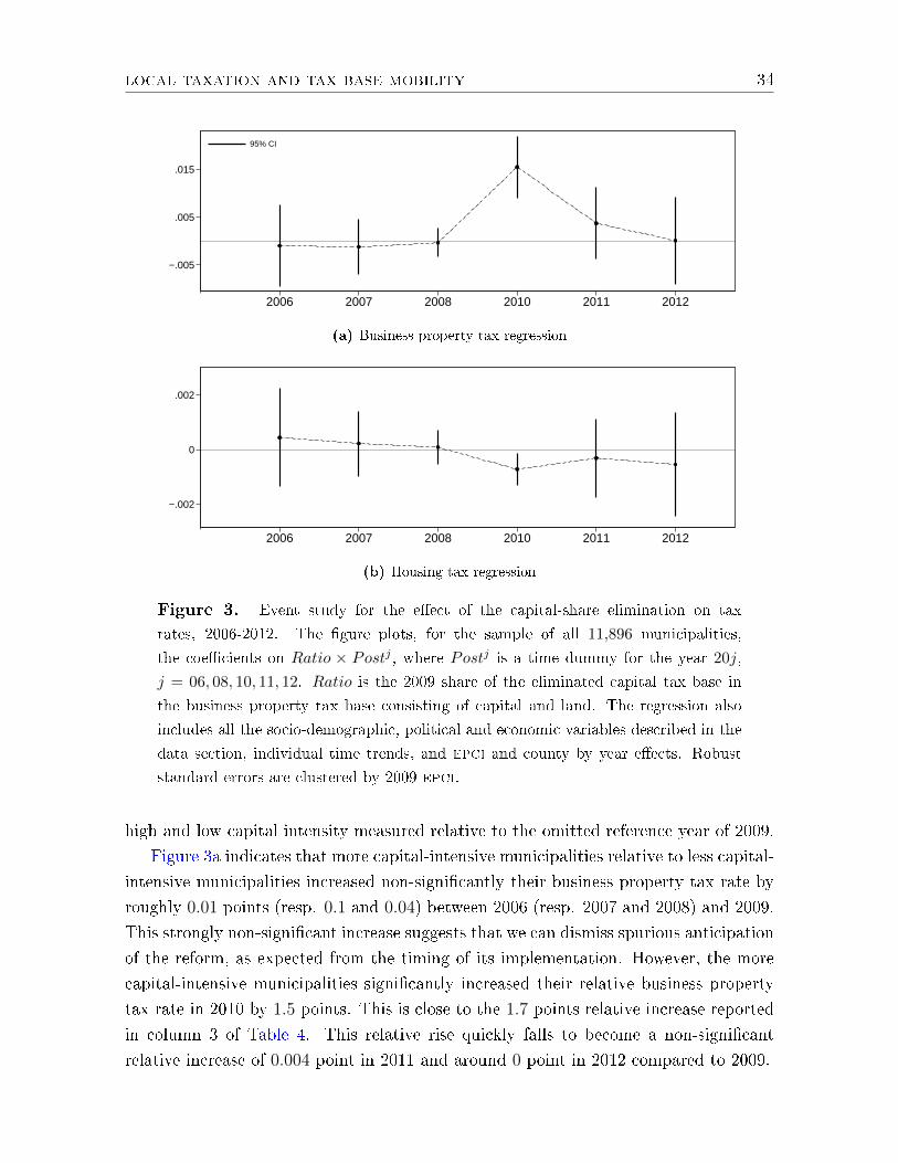
local taxation and tax base mobility 34
−.005
.005
.015
2006 2007 2008 2010 2011 2012
95% CI
(a) Business property tax regression
−.002
0
.002
2006 2007 2008 2010 2011 2012
(b) Housing tax regression
Figure 3. Event study for the e�ect of the capital-share elimination on tax
rates, 2006-2012. The �gure plots, for the sample of all 11,896 municipalities,
the coe�cients on Ratio × Postj , where Postj is a time dummy for the year 20j,
j = 06, 08, 10, 11, 12. Ratio is the 2009 share of the eliminated capital tax base in
the business property tax base consisting of capital and land. The regression also
includes all the socio-demographic, political and economic variables described in the
data section, individual time trends, and epci and county by year e�ects. Robust
standard errors are clustered by 2009 epci.
high and low capital intensity measured relative to the omitted reference year of 2009.
Figure 3a indicates that more capital-intensive municipalities relative to less capital-
intensive municipalities increased non-signi�cantly their business property tax rate by
roughly 0.01 points (resp. 0.1 and 0.04) between 2006 (resp. 2007 and 2008) and 2009.
This strongly non-signi�cant increase suggests that we can dismiss spurious anticipation
of the reform, as expected from the timing of its implementation. However, the more
capital-intensive municipalities signi�cantly increased their relative business property
tax rate in 2010 by 1.5 points. This is close to the 1.7 points relative increase reported
in column 3 of Table 4. This relative rise quickly falls to become a non-signi�cant
relative increase of 0.004 point in 2011 and around 0 point in 2012 compared to 2009.

local taxation and tax base mobility 35
The evolution of the housing tax rate in more capital-intensive municipalities relative
to less capital-intensive ones is fairly symmetric. It decreases non-signi�cantly by less
than 0.045 points between 2006 (resp. 2007 and 2008) and 2009. It knows a slightly
signi�cant decrease of 0.07 points in 2010 (a bit lower than the 0.12 points in Table 4).
At the end of the sample period in 2011 and 2012 the relative housing tax rate decreases
are non-signi�cant. The most important evidence from the Figure 3 is that the event-
study estimates reject signi�cant e�ects of the reform prior to its implementation. Thus,
the reform can be regarded as unanticipated by municipalities, which reinforces our DD
identifying assumption.
6.3. Variation across municipality types
By aggregating the full sample of municipalities, the results presented above potentially
hide heterogeneous e�ects of removal of the capital tax base on municipal tax rates.
Table 5 explores this possible heterogeneity in treatment e�ect across three municipal
characteristics: (non-)metropolitan, ideology and high/low new business tax revenue.
It reports the baseline estimates of equation (4.1) for the most demanding speci�cation
comprising controls and epci and county by year e�ects, for six municipality sub-
samples. Columns 1 and 2 present the estimates for metropolitan and non-metropolitan
municipalities. Columns 3 and 4 report the respective results for municipalities where
the majority voted for a left-wing candidate and a right-wing candidate in the 2007
presidential election. Columns 5 and 6 distinguish between municipalities collecting
higher (above the 2011 median) and lower (below the 2011 median) new business tax
revenues per capita after 2011. For each of these sub-samples, we report the treatment
e�ect estimates on the interaction Ratio×Post when the dependent variable is business
property tax and when it is the housing tax. We also report the sub-sample means for
these two tax rates and the capital share in the business property tax base in 2009.
For easier comparison of the treatment e�ect among sub-samples, we report each sub-
sample average treatment e�ect (ATE) relative to the mean related tax rate of 2009.56
A �rst look at the estimated treatment e�ects in Table 5 shows that the coe�cients
(although not all signi�cant) have the expected signs. That is, in each sub-sample, mu-
nicipalities which had larger capital share of their pre-reform business property tax base
removed, responded by increasing their business property tax rate and decreasing their
housing tax rate relative to less capital-intensive municipalities. However, we observe
substantial di�erences among sub-groups which call for further discussion. Columns
56 As usual, the ATE is computed by multiplying the point estimates on Post × Ratio by the
sub-sample average capital share in 2009.

local taxation and tax base mobility 36
1 and 2 indicate that the treatment e�ect on the business property tax rate is much
lower for municipalities located in a metropolitan area compared to non-metropolitan
municipalities: it represents only 2.3% of the tax rate of 2009 for the former and 16.7%
for the latter. This suggests that capital mobility exerts a weaker downward pressure
on business tax rates in metropolitan areas. This result supports one of the main re-
sults in the agglomeration economies literature which suggests that the existence of
agglomeration rents in metropolitan areas tends to mitigate the tax competition re-
sult that capital mobility spurs local governments to lower their business tax rate.57
The treatment e�ect of capital share removal is also lower (and non-signi�cant)in the
housing tax rate regression for municipalities in metropolitan areas compared to others:
respectively −2% and −4.3% of the 2009 tax rate for the �rst and second sub-samples.
This suggests that comparison of higher and lower capital-intensive municipalities re-
veals a weaker rebalancing of the tax burden from businesses to residents following the
decrease in capital mobility in metropolitan areas.
Columns 3 and 4 in Table 5 show that municipalities with higher capital shares
increased their business property tax rate relatively less if they included a majority
of left-wing voters. Indeed, the (non-signi�cant) estimate of 0.004 on Ratio × Post
for left-wing jurisdictions is lower than the strongly signi�cant estimate of 0.01 for
right-wing ones. This di�erence is re�ected also in the ATE relative to the tax rate
voted in 2009 (2.9% for left wing municipalities against 8.8% for right wing ones). This
�nding suggests that ideology matters for the response of voted business tax rate to
capital mobility. Left-leaning municipalities appear to be less sensitive to the downward
pressure exerted by mobile capital. The treatment e�ect on housing is also interesting
since in contrast to what we observed for the business property tax rate, left-wing
municipalities with a more capital-intensive tax base prior to reform appear to reduce
their tax rate to the same extent as their right-wing counterparts. Indeed, the ATE
represents −4.08% of their 2009 tax rate and −4.06% of right-wing municipalities. This
result can be interpreted as a sign that left-wing municipalities are ceteris paribus more
prone (compared to right-wing ones) to alleviate the tax burden on households.58
57 See the seminal theoretical paper by Baldwin and Krugman (2004). Contributions providing
empirical evidence are, e.g., Charlot and Paty (2010), Luthi and Schmidheiny (2013) and Fréret and
Maguain (2017).58 Although these preliminary �ndings call for deeper analysis, they are informative in regard of the
contrasting results obtained in the political economy studies dealing with the link between ideology
and local taxation. Indeed, while e.g. Pettersson-Lidbom (2008) �nds empirical evidence of the impact
of ideology on local tax level in the case of Swedish municipalities, Ferreira and Gyourko (2009) point
out the �striking lack of partisan impact at the local level� in a study of American municipalities.

local taxation and tax base mobility 37
Table 5. Business property tax and housing tax regressions with two-period treatment.
Metropolitan Ideology New Revenue
Yes No Left Right High Low
(1) (2) (3) (4) (5) (6)
A. Business property tax regression
Ratio× Post 0.00271* 0.02110*** 0.00411 0.00990*** 0.00082* 0.00849**
(0.00115) (0.00490) (0.00216) (0.00278) (0.00035) (0.00278)
Mean tax rate 2009 .0951 .0986 .1138 .0905 .1036 .0883
ATE relative to
tax rate 2009
.0231 .1674 .0285 .0881 .0065 .0743
B. Housing tax regression
Ratio× Post -0.00209 -0.00418* -0.00444* -0.00409*** -0.00398 -0.00419***
(0.00118) (0.00181) (0.00174) (0.00116) (0.00234) (0.00114)
Mean tax rate 2009 .0844 .076 .086 .0812 .0904 .0743
ATE relative to tax rate
tax rate 2009
-.02 -.0431 -.0408 -.0406 -.0365 -.0436
Capital share 2009 .808 .7824 .7906 .8052 .83 .7736
Municipalities 9001 2895 2786 9110 5948 5948
Note.�Each pair of sub-samples comprises all 11,896 municipalities from 2006 to 2012. Ratio
is the 2009 share of the eliminated capital tax base in the business property tax base consisting
in capital and land. Post is an indicator for post-reform years 2010-2012. The regressions also
include all the socio-demographic, political and economic variables described in the data section,
individual time trends, and epci and county by year e�ects. Sub-samples high and low new revenue
are municipalities collecting per capita new business tax revenue � cvae + ifer + tascom �
above and below the sample median. Robust standard errors clustered by 2009 epci are reported
in parentheses. ∗ p < .05, ∗∗ p < .01, ∗∗∗ p < .001.
Finally, columns 5 and 6 in Table 5 distinguish municipalities collecting per capita
new business tax revenues in 2011 above the sample median and those whose new busi-
ness tax revenues are below the median.59 Since municipalities have no decision power
on the vote for these new business taxes which rely on the value-added generated by lo-
cal �rms (cvae) and their size and sector (ifer and tascom), they receive high or low
new business tax revenues depending on their economic structure. Comparison of the
59 The new business tax revenues are the sum of the cvae, the ifer and the tascom (see section 3
for de�nitions). We divide these revenues by the municipal population for the sake of comparability.

local taxation and tax base mobility 38
last two columns in Table 5 reveals that more capital-intensive municipalities (relative
to less capital intensive ones) collecting high tax revenues from the new business taxes
after the reform are able to raise their business property tax rates much less than their
counterparts that collected lower new tax revenues. Indeed, the respective ATE relative
to the 2009 tax rate of 0.65% and 7.43% indicates that municipalities with important
new tax revenues responded substantially less to the reduced downward pressure in-
duced by elimination of the mobile capital tax base. This result makes economic sense.
While capital now does not �gure in the business property tax base, these municipalities
cannot charge overly high taxes on business land since this might cause �rms to move
and have important negative e�ects on the revenues from the new business taxes.60 Fi-
nally, we see that removing the capital share gave these municipalities with higher new
business tax revenues less latitude to cut their housing tax rate: their ATE relative to
the 2009 tax rate is of −3.65% compared to −4.36% for the other municipalities. This
can be viewed as a sign that their lower ability of increasing business property tax rates
in response to the reform allow lower leeway to reduce the tax burden on residents.
7. Conclusion
This paper examined the relationship between tax base mobility and local taxation
through theoretical and empirical analyses. The theoretical model derived local tax
setting equations, which showed that decreasing the capital intensity of the business
property tax base increases the business property tax rates and decreases the tax on
residents. We tested this result using a French reform implemented in 2010 which
changed the composition of the main local business tax base to reliance on a much less
mobile tax base and implemented compensation for the tax base loss. The results of
the empirical analysis are consistent with the theoretical predictions, and suggest that
reducing the mobility of the tax base results in higher business property tax rates. Also,
housing tax rates are negatively a�ected by the reform.
In terms of public policy implications, we show that the composition of the local tax
base has a clear impact on the related tax decisions. Although exact compensation was
paid to the municipalities after the reform, local governments seized the opportunity
to increase their tax rates on a less mobile tax base. However, since we do not know
whether local business tax rates were initially lower or higher than the optimal level,
we cannot draw conclusions as to the e�ciency of the reform.
60 Recall that the new business taxes (cvae, ifer and tascom) are note voted for by the munici-
palities. They only depend on the type and size of �rms they host.
REFERENCES 39
Our analysis points to the need for more theoretical and empirical investigations of
tax base reforms. A similar reform of the French national tax system is currently being
discussed in France. Indeed, in the Draft Budget Bill for 2018, government proposed
removing the most mobile part (based on capital) of the solidarity tax base on wealth
ISF (initially based on capital and real property). We can expect this reform to produce
a higher tax rate on the immobile tax base of the new ISF (real property), called tax
on real property wealth (IFI). Unlike the business property tax reform studied in this
paper, this increase would be due to both a capital-mobility e�ect and a budgetary
e�ect since the draft budget bill does not stipulate complete budget compensation.
References
Allers, M. A. and J. P. Elhorst (2005). Tax mimicking and yardstick competition among
local governments in the netherlands. International tax and public �nance 12 (4),
493�513.
Baldwin, R. E. and P. Krugman (2004). Agglomeration, integration and tax harmoni-
sation. European Economic Review 48 (1), 1�23.
Boadway, R. W. and D. E. Wildasin (1984). Public sector economics. Little, Brown.
Bouvier, M. (2018). Les �nances locales.
Braid, R. M. (1996). Symmetric Tax Competition with Multiple Jurisdictions in Each
Metropolitan Area. American Economic Review 86 (5), 1279�90.
Bretschger, L. and F. Hettich (2002). Globalisation, capital mobility and tax compe-
tition: theory and evidence for oecd countries. European journal of political econ-
omy 18 (4), 695�716.
Brueckner, J. K. (2000). A Tiebout/tax-competition model. Journal of Public Eco-
nomics 77 (2), 285�306.
Brueckner, J. K. and H.-A. Kim (2003). Urban sprawl and the property tax. Interna-
tional Tax and Public Finance 10 (1), 5�23.
Brueckner, J. K. and L. A. Saavedra (2001). Do Local Governments Engage in Strategic
Property-Tax Competition? National Tax Journal 54 (n. 2), 203�30.
Card, D. (1992). Using regional variation in wages to measure the e�ects of the federal
minimum wage. Industrial & Labor Relations Review 46 (1), 22�37.

REFERENCES 40
Carlsen, F., B. Langset, and J. Rattsø (2005). The relationship between �rm mobility
and tax level: Empirical evidence of �scal competition between local governments.
Charlot, S. and S. Paty (2007). Market access e�ect and local tax setting: evidence
from french panel data. Journal of Economic Geography .
Charlot, S. and S. Paty (2010). Do agglomeration forces strengthen tax interactions?
Urban Studies .
Ferreira, F. and J. Gyourko (2009). Do political parties matter? evidence from us cities.
The Quarterly journal of economics 124 (1), 399�422.
Fisher, R. C. (2015). State and local public �nance, chicago: Richard d. irwin.
Fréret, S. and D. Maguain (2017). The e�ects of agglomeration on tax competition:
evidence from a two-regime spatial panel model on french data. International Tax
and Public Finance, 1�41.
Gaigné, C., S. Riou, and J.-F. Thisse (2016). How to make the metropolitan area work?
neither big government, nor laissez-faire. Journal of Public Economics 134, 100�113.
Guené, C. (2012). De la taxe professionnelle á la contribution économique territoriale
: 25 propositions pour une transition. Rapport d'information numéro 611 .
Hauptmeier, S., F. Mittermaier, and J. Rincke (2012). Fiscal competition over taxes
and public inputs. Regional science and urban economics 42 (3), 407�419.
Luthi, E. and K. Schmidheiny (2013). The e�ect of agglomeration size on local taxes.
Journal of Economic Geography 14 (2), 265�287.
Ly, T. (2018). Sub-metropolitan tax competition with household and capital mobility.
International Tax and Public Finance 25 (5), 1129�1169.
Lyytikäinen, T. (2012). Tax competition among local governments: Evidence from a
property tax reform in �nland. Journal of Public Economics 96 (7), 584�595.
Oates, W. E. (1972). Fiscal federalism. Books .
OCDE (2013). OECD Regions at a Glance 2013.
Pettersson-Lidbom, P. (2008). Do parties matter for economic outcomes? a regression-
discontinuity approach. Journal of the European Economic Association 6 (5), 1037�
1056.
41
Quinn, D. (1997). The correlates of change in international �nancial regulation. Amer-
ican Political science review 91 (3), 531�551.
Revelli, F. (2005). On spatial public �nance empirics. International Tax and Public
Finance 12 (4), 475�492.
Richter, W. F. and D. Wellisch (1996). The provision of local public goods and factors
in the presence of �rm and household mobility. Journal of Public Economics 60 (1),
73�93.
Slemrod, J. (2004). Are corporate tax rates, or countries, converging? Journal of Public
Economics 88 (6), 1169�1186.
Sta�ord, J. and L. DeBoer (2014). The personal poroperty tax in indiana: Its reduction
or elimination is no simple task. Indiana Fiscal Policy Institute.
Tiebout, C. M. (1956). A Pure Theory of Local Expenditures. Journal of Political
Economy 64, 416.
Wellisch, D. (2006). Theory of Public Finance in a Federal State. Number
9780521026871 in Cambridge Books. Cambridge University Press.
Wellisch, D. and J. Hulshorst (2000). A Second-Best Theory of Local Government
Policy. International Tax and Public Finance 7 (1), 5�22.
Wildasin, D. E. (1989). Interjurisdictional capital mobility: Fiscal externality and a
corrective subsidy. Journal of urban economics 25 (2), 193�212.
Wilson, J. D. (1986). A theory of interregional tax competition. Journal of Urban
Economics 19 (3), 296�315.
Wilson, J. D. (1995). Mobile Labor, Multiple Tax Instruments, and Tax Competition.
Journal of Urban Economics 38 (3), 333�356.
Wilson, J. D. (1999). Theories of Tax Competition. National Tax Journal 52 (n. 2),
269�304.
Wilson, J. D. and D. E. Wildasin (2004). Capital tax competition: bane or boon.
Journal of public economics 88 (6), 1065�1091.
Zodrow, G. R. and P. Mieszkowski (1986). Pigou, Tiebout, property taxation, and the
underprovision of local public goods. Journal of Urban Economics 19 (3), 356�370.

42
Appendix A Derivation of the local public policy rules
The purpose of this appendix section is, �rst, to derive the optimal ta conditions (tr0),
(bc0), (tr0) and (tr1) (Public policy rules),61 which requires to characterize the �rst-
order conditions of the local government (First-order conditions), as well as the location
responses of resident and capital to local policy changes (Location responses) .The sec-
ond objective of this appendix section is to derive the tax rate change conditions (2.10a)
and (2.10b) in the presence of a perfect revenue compensation (Tax rate evolution in
the presence of a revenue compensation). We focus on the representative jurisdiction i
in all this appendix. We drop index i for notational convenience.
A.1 First-order conditions
The benevolent local government maximizes the utility of its residents U ≡U(x,G,R) = x + α log(G/R) which, by substituting x using (2.1), can be written
as:
U =rK + ρ`+ (n− 1)ρ`
P+ α log
(G
R
)− ρ− τR,
where ρ ≡ ρj with j 6= i denotes the other municipalities' land rent. Using respectively
(2.2) and (2.4) to substitute τR and `, we obtain:
U =rK + ρR + ρL+ (n− 1)ρ¯
P+ u. (A.1)
Since F is homogeneous of degree 1, Euler's theorem requires that F = KFK + LFL,
where subscripts stand for derivatives. Inserting (2.3) into this condition implies the
zero-pro�t condition F i(Ki, Li) − [r + (1 − θ)τPi ]Ki − (ρi + τPi )Li = 0. Replacing ρR
and ρL into (A.1) using respectively (2.2) and the zero-pro�t condition yields:
U =
[α log
(GR
)− τR − u
]R + F −
[r + τP (1− θ)
]K − τPL+ rK + (n− 1)ρ¯
P+ u
From the household budget constraint (2.1), it follows that the local government ob-
jective can be written as:
U =F (K, `−R)− rK +
[α log
(GR
)− u]R−G− f + θΛ + rK + (n− 1)ρ¯
P+ u
(A.2)
where L has been substituted in the production function using (2.1).
61 To this aim, we follow standard computational steps. See e.g. Wellisch (2006).
43
In the sequel, we assume without loss of generality that the local government freely
chooses τR and G while adjusting τP to clear its budget constraint (2.5).62 Since house-
hold and capital locations are not under the direct control of the local government, a
rational government must take account of location responses to its policy. The responses
of residents (∂R/∂τR and ∂R/∂G) and capital (∂K/∂τR and ∂K/∂G) to changes in the
local government's policy instruments can be derived from the migration equilibrium
condition (2.2) and the necessary conditions for the optimal demand for capital (2.3a)
from local �rms. Inserting (2.4) and (2.3b) into (2.2) and (2.3a) and substituting τP
using the budget constraint (2.5) the following two-equation system results:
FK(K, `−R)− G+ f − θΛ− τRR(1− θ)K + `−R
(1− θ)− r = 0 (A.3)
α log
(G
R
)− FL(K, `−R)− τR +
G+ f − θΛ− τRR(1− θ)K + `−R
− u = 0 (A.4)
The location system allows to derive R and K as implicit functions of τR and G.
Let us now determine the �rst-order conditions of the local government. Di�erenti-
ating (A.2) with respect to t ∈ {τR, G}, we have ∂U/∂t = 0 is equivalent to:
[FK − r]∂K
∂t+
[α log
(G
R
)− u− FL − α
]∂R
∂t+
(αR
G− 1
)∂G
∂t= 0.
Replacing u, FK and FL using (2.2), (2.3a) and (2.3b) and collecting terms, the following
�rst-order conditions result:
(τR − τP − α)∂R
∂τR+ τP (1− θ) ∂K
∂τR= 0 (A.5)
(τR − τP − α)∂R
∂G+ τP (1− θ)∂K
∂G+ α
R
G− 1 = 0 (A.6)
A.2 Location responses
We now determine the location responses of residents and capital. To this aim, we
di�erentiate (A.3) and (A.4) with respect to t ∈ {τR; τP}, which yields in matrix form:
A
(∂R∂t∂K∂t
)= B
where
62 This assumption allows to solve the model without introducing a Lagrange multiplier for the
budget constraint of the local government. Note that whatever the instrument chosen to clear the
budget (τR, τP of G), the results are strictly identical.

44
A ≡
((1−θ)(τR−τP )(1−θ)K+`−R − FKL FKK + τP (1−θ)2
(1−θ)K+`−R
− αR
+ FLL − τR−τP(1−θ)K+`−R − τP (1−θ)
(1−θ)K+`−R − FLK
)(A.7)
and
B ≡
(1−θ)(1−θ)K+`−R
[∂G∂t−R∂τR
∂t
][1 + R
(1−θ)K+`−R
]∂τR
∂t−[
1(1−θ)K+`−R + α
G
]∂G∂t
(A.8)
Then, from Cramer's rule:
∂R
∂t= |A|−1
∣∣∣∣∣∣(1−θ)
(1−θ)K+`−R
[∂G∂t−R∂τR
∂t
]FKK + τP (1−θ)2
(1−θ)K+`−R[1 + R
(1−θ)K+`−R
]∂τR
∂t−[
1(1−θ)K+`−R + α
G
]∂G∂t− τP (1−θ)
(1−θ)K+`−R − FLK
∣∣∣∣∣∣ ,(A.9)
∂K
∂t= |A|−1
∣∣∣∣∣∣(1−θ)(τR−τP )(1−θ)K+`−R − FKL
(1−θ)(1−θ)K+`−R
[∂G∂t−R∂τR
∂t
]− αR
+ FLL − τR−τP(1−θ)K+`−R
[1 + R
(1−θ)K+`−R
]∂τR
∂t−[
1(1−θ)K+`−R + α
G
]∂G∂t
∣∣∣∣∣∣(A.10)
where |A| is the determinant of A, and for all t ∈ {τR;G}, ∂t/∂t′ is 1 if t = t′ and 0
otherwise.
A.3 Public policy rules
We can now determine the public policy rules by inserting the location responses (A.9)
and (A.10) into the �rst-order conditions (A.5) and (A.6). Let us start with the taxation
rules (tr0) and (tr1). Replacing t by τR in the location responses and inserting them
into (A.5), we obtain:63∣∣∣∣∣∣− (1−θ)R
(1−θ)K+`−R FKK
[(τR − τP − α) + FKL
FKKτP (1− θ)
]− α τP (1−θ)2
(1−θ)K+`−R
1 + R(1−θ)K+`−R −FLK
[(τR − τP − α) + FLL
FLKτP (1− θ)
]+[1 + R
(1−θ)K+`−R
]αRτP (1− θ)
∣∣∣∣∣∣ = 0.
Applying the column operation C2← C2− αRτP (1−θ)×C1 and noticing FKL
FKK= FLL
FLK=
−KLthe derivative of F are homogeneous of degree 0, we obtain:∣∣∣∣∣∣
− (1−θ)R(1−θ)K+`−R FKK
(1−θ)K+`(1−θ)K+`−R −FLK
∣∣∣∣∣∣[τR − τP − α− K
LτP (1− θ)
]= 0.
63 Recall that from usual determinant computation rules, we have:
α
∣∣∣∣∣a c
b d
∣∣∣∣∣+ βα
∣∣∣∣∣e a
f b
∣∣∣∣∣ = α
∣∣∣∣∣a αc− βeb αb− βf
∣∣∣∣∣ .

45
The determinant is negative due to the standard assumption FKK < 0 (which implies
FKL > 0 by homogeneity F ) so that:
τR − τP − α− K
LτP (1− θ) = 0 (A.11)
which is precisely the taxation rule (tr0), for θ = 0 and (tr1), for θ = 1.
We now derive the local public good provision rule.64 Replacing t by G in the
location responses and inserting them into (A.6), and following the same computation
step as above, it follows that:∣∣∣∣∣∣1−θ
(1−θ)K+`−R FKK[(τR − τP − α)− K
LτP (1− θ)
]− α τP (1−θ)2
(1−θ)K+`−R
− 1(1−θ)K+`−R −
αG−FLK
[(τR − τP − α)− K
LτP (1− θ)
]+[1 + R
(1−θ)K+`−R
]αRτP (1− θ)
∣∣∣∣∣∣+
(αR
G− 1
)|A| = 0
Using (A.11) to simplify and applying the column operation C2← C2+GRτP (1−θ)×C1,
we obtain: ∣∣∣∣∣∣1−θ
(1−θ)K+`−R − τP (1−θ)2(1−θ)K+`−R
(α− G
R
)− 1
(1−θ)K+`−R −αG
τP (1−θ)(1−θ)K+`−R
(α− G
R
)∣∣∣∣∣∣+
(αR
G− 1
)|A| = 0
which gives: (αR
G− 1
)[|A| − α
R
τP (1− θ)2
(1− θ)K + `−R
]= 0 (A.12)
Yet, replacing replacing τR from (A.11) in A as de�ned by (A.7) and developing its
determinant, we obtain after some simple manipulations:
|A| = α
R
τP (1− θ)2
(1− θ)K + `−R+
α`
RLFKK (A.13)
which shows that the term between square brackets (A.12) is non zero, so that the
government public good policy is characterized by:
αR
G= 1 (A.14)
which is the well-known Samuelson rule (see footnote 18).
We can now derive the budget constraint rules (bc0) and (bc1). Inserting (A.14)
into the local government budget constraint (2.5) and solving for τP , we obtain:
τP =R
(1− θ)K + L
(α− τR +
f − Λ
R
)which is precisely the taxation rule (bc0), for θ = 0 and (bc1), for θ = 1.
64 Public good provision is rather peripheral in this paper, but deriving the public good provision
rule is necessary to derive the tax reduced forms.
46
A.4 Tax rate evolution in the presence of a revenue compensation
In this last subsection, we derive the tax rate change equations (2.10a) and (2.10b). In
the presence of a revenue compensation Λ = τP0K0, from (2.8b) and (2.8a), we have:
τP1 − τP0 =f
`− τP0K0
`− (1− κ0)f
`
Substituting τP0 and ` using (2.8a) and (2.4), replacing κ0 by its de�nition (ie.
K0/(K0 + L0)) we obtain:
τP1 − τP0 =(R0 + L0)(K0 + L0)− (R0 + L0 +K0)L0
K0 + L0
f
`2= R0 f
`2K0
K0 + L0=PLf
`κ0,
(A.15)
where the last equality is obtained using the de�nition of κ0, recalling that R0 = Pin the symmetric equilibrium and that by de�nition n` = L. This proves the tax rate
change equation (2.10a).
Let us now turn to evolution of the tax on resident. Replacing τP0 using (2.8a) into
(2.7a), we have:
τR0 = α + τP0 +f
`κ0 (A.16)
Besides, using (A.15) so substitute τP1 into (2.7b) yields:
τR1 = α + τP0 +PLf
`κ0 (A.17)
Finally, the di�erence between (A.17) and (A.16) gives the tax rate change equation
(2.10b).
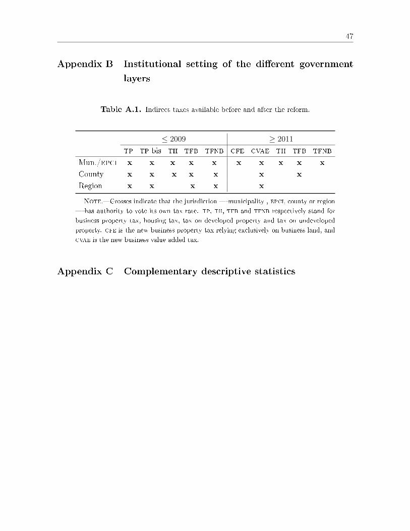
47
Appendix B Institutional setting of the di�erent government
layers
Table A.1. Indirect taxes available before and after the reform.
≤ 2009 ≥ 2011
tp tp bis th tfb tfnb cfe cvae th tfb tfnb
Mun./epci x x x x x x x x x x
County x x x x x x x
Region x x x x x
Note.�Crosses indicate that the jurisdiction � municipality , epci, county or region
� has authority to vote its own tax rate. tp, th, tfb and tfnb respectively stand for
business property tax, housing tax, tax on developed property and tax on undeveloped
property. cfe is the new business property tax relying exclusively on business land, and
cvae is the new business value added tax.
Appendix C Complementary descriptive statistics

48
Table A.2. Descriptive statistics on control variables in 2009.
Mean Standarddeviation
Minimum Maximum
Municipal characteristics
Population (in thousands) 1.3 20.8 .009 2234
Density 0.1 0.7 3.5e-04 26
Number of �rms per inhabitant 0.1 0.1 .012 .95
Metropolitan (dummy) 0.8 0.4 0 1
Median income (in 10,000 e) 1.8 0.3 .91 5.4
Share of commuters (%) 74.7 14.6 3.7 100
Share of left-wing voters (%) 42.4 10.9 0 94
Share of population below 15 year old (%) 32.7 6.0 2.9 68
Schooling rate (%) 92.9 4.1 50 100
Share of population per SPC (%)
Farmers 3.9 5.1 0 67
Craftsmen 4.2 3.2 0 50
Managers 5.0 4.3 0 57
Temporary workers 12.2 6.0 0 100
Employees 15.4 5.4 0 65
Blue color workers 16.4 7.0 0 67
Retirees 30.1 10.1 0 100
Unemployed 12.9 5.3 0 80
Share of �rms per sector (%)
Industry 44.3 20.6 0 98
Fincance and real estate 2.2 3.1 0 50
Trade and retail 12.5 8.2 0 67
Other tertiary sector 26.7 13.2 1.4 100
Share of �rms per size (%)
No employee 70.4 12.5 0 100
Less than 10 employees 25.9 10.8 0 100
At least 10 employees 3.7 4.5 0 54
Note.�The sample includes all 11,896 municipalities for the year 2009. Density is the number of
inhabitants (in thousands) per square kilometer. Share of left-wing voters is that of the presidential
election of 2007. Schooling rate is the share of population below 17 year old enrolled in school.

49
Table A.3. Descriptive statistics per category of capital share intensity.
2006 2007 2008 2009 2010 2011 2012
A. Capital share below the median
Capital share.6909(.2243)
.6891(.2253)
.6859(.2288)
.6741(.2364)
Business property tax rate.1007(.0574)
.1007(.0575)
.1011(.0578)
.1013(.0584)
.184(.0683)
.1857(.0665)
.1869(.0665)
Housing tax rate.0867(.0374)
.0869(.0374)
.0874(.0376)
.0883(.0379)
.089(.0403)
.1578(.0496)
.1584(.0499)
Observations 5948 5948 5948 5948 5948 5948 5948
B. Capital share above the median
Capital share.9098(.0675)
.9161(.0582)
.9229(.0448)
.9294(.0354)
Business property tax rate.0897(.0466)
.0897(.0467)
.0901(.0467)
.0906(.0467)
.1749(.0535)
.1746(.0549)
.1756(.0555)
Housing tax rate.075(.0347)
.0751(.0347)
.0757(.0349)
.0764(.0351)
.0769(.0373)
.1453(.0477)
.146(.0481)
Observations 5948 5948 5948 5948 5948 5948 5948
Note.�Each cell contains the variable mean and standard error in parentheses. Panel
A (resp. Panel B) describe municipalities with a share of capital in the business property
tax below (resp. above) the median. The sample median of the capital share in 2009 is
86.76%.

50
Table A.4. Correlation between net and gross business property tax base.
Year Pearson'scoe�cient
Spearman'scoe�cient
2006 99.9949 99.3043
2007 99.9945 99.319
2008 99.9931 99.3118
2009 99.9928 99.2703
2010 99.981 97.2859
2011 99.9787 97.2934
2012 99.9836 97.5448
Note.�N=11,896. The table re-
ports correlation coe�cients between
the gross tax base GB and the net
tax base NB of the business property
tax. In the pre-reform years 2006-
2009, GB = K+L and NB = αKK+
αLL, where K (resp. L) is the capital
(resp. business land) tax base, and αK
(resp. αL) is the share of the tax base
not exempted from tax. In the post-
reform years 2010-2012, GB = L and
NB = αLL. The signi�cance tests for
all coe�cients are below 10−6, so that
they strongly reject non signi�cance of
the correlation.

51
Appendix D Event study estimates
Table A.5. Event study coe�cients for the continuous and discrete regressions.
Dependent variable: Dependent variable:
Business property tax Housing tax
Coef. 95%CI Coef. 95%CI
A. Continuous treatment
Ratio× Post06 −.00096 [−.00949 ; .00757] .00045 [−.00133 ; .00223]
Ratio× Post07 −.00123 [−.00706 ; .0046] .00023 [−.00097 ; .00142]
Ratio× Post08 −.00036 [−.00339 ; .00268] .00009 [−.00053 ; .0007]
Ratio× Post10 .01552 [.00907 ; .02197] −.00072 [−.00132 ; −.00013]
Ratio× Post11 .00371 [−.0038 ; .01123] −.00031 [−.00175 ; .00113]
Ratio× Post12 .00009 [−.00909 ; .00926] −.00054 [−.00245 ; .00136]
B. Discrete treatment
High× Post06 .00045 [−.00027 ; .00116] .00041 [−.00015 ; .00097]
High× Post07 .00016 [−.00038 ; .00069] .00026 [−.00013 ; .00065]
High× Post08 −.00019 [−.00055 ; .00017] .00021 [−.00002 ; .00044]
High× Post10 .00129 [.00027 ; .00231] −.00031 [−.00053 ; −.00009]
High× Post11 −.00075 [−.00188 ; .00038] −.00075 [−.00183 ; .00033]
High× Post12 −.00136 [−.00258 ; −.00014] −.00086 [−.00201 ; .00028]
Note.�The sample is all 11,896 municipalities from 2006 to 2012. The table
reports the coe�cients on Ratio×Postj and High×Postj of respectively the contin-uous and discrete event-study regressions. Postj is a time dummy for the year 20j,
j = 06, 08, 10, 11, 12. Ratio is the 2009 share of the eliminated capital tax base in
the business property tax base consisting in capital and land. High is an indicator
equal to one if a municipality has a 2009 capital share above the sample median, and
zero otherwise. The regression also includes all the socio-demographic, political and
economic variables described in the data section, individual time trends, and epci and
county by year e�ects. Robust standard errors are clustered by 2009 epci.
Related Documents