Local stability of limit cycles for MIMO relay feedback systems

a

sys-e map

tury [7].o con-0] andis thatIt is

uisite

feed-ee [1,4]t cy-issue

J. Math. Anal. Appl. 288 (2003) 112–123

www.elsevier.com/locate/jma

Local stability of limit cycles for MIMO relayfeedback systems

Chong Lin,∗ Qing-Guo Wang, and Tong Heng Lee

Department of Electrical and Computer Engineering, National University of Singapore, Singapore 119260

Received 26 February 2003

Submitted by M. Iannelli

Abstract

This paper concerns with the local stability of limit cycles for decentralized relay feedbacktems. It presents a sufficient condition for the local stability based on the well-known Poincarmethod. The effectiveness of the presented result is illustrated by a numerical example. 2003 Elsevier Inc. All rights reserved.

Keywords: Decentralized relay feedback; Hysteresis; Limit cycles; Local stability

1. Introduction

Relay feedback has attracted considerable research attention for more than cenApplications of relay systems range from stationary control of industrial processes ttrol of mobile objects. Recent advances are relay auto-tuning of PID controllers [2,1process identification and control [9]. A phenomenon of relay feedback systemsa particular type of periodic motions, i.e., limit cycle, may occur in the trajectories.meaningful to determine the stability of a limit cycle since this property is a pre-reqin engineering applications.

For single-input single-output plants with a single relay element, say, SISO relayback systems, exact method has been developed to analyze limit cycle behaviors, sand references therein. Astrom [1] gives elegant criteria for the local stability of limicles by considering the linear approximation of the Poincare map. The global stabilityis studied in [4].

* Corresponding author.E-mail address: [email protected] (C. Lin).

0022-247X/$ – see front matter 2003 Elsevier Inc. All rights reserved.doi:10.1016/S0022-247X(03)00582-1

C. Lin et al. / J. Math. Anal. Appl. 288 (2003) 112–123 113

andf multi-relayyclesbasedrelayecen-ystemclosed-

layhe exactck theeters

t givenideredormulat con-n 5

The

r

ere,elyt

Practically and theoretically, multi-input multi-output systems are more commonuseful, see [8,9] for details. Recent advances also show the important applications oinput multi-output systems connected with decentralized relays which called MIMOfeedback systems [8,9]. So far, there are few efforts devoted to the study of limit cfor MIMO relay feedback systems. Palmor et al. [5,6] present a frequency domainmethod for evaluating the periods and the stability of limit cycles in decentralizedsystems. TheZ-transform technique is employed therein to convert the continuous dtralized relay system under a limit cycle to an equivalent fictitious sampled-data swith synchronous samplers. Then, regular sampled-data tools are applied to deriveform necessary conditions as well as stability conditions.

In this paper, we will revisit the local stability of limit cycles for decentralized resystems through exact method. The analysis is state-space based and takes into tconsideration of the Poincare map. The result is novel in the sense that it is to cheSchur stability of a certain matrix which is constructed by the original system paramand the limit cycle parameters. The criterion can be viewed as a generalization of thain [1] for SISO systems. This paper is organized as follows. In Section 2, the consdecentralized relay system and problem are formulated. Section 3 gives a closed ffor computing the period of the considered limit cycle. Section 4 presents a sufficiendition for the local stability of the limit cycle. A numerical example is given in Sectioto illustrate our result. This paper is concluded in Section 6.

2. Problem formulation and preliminaries

The multi-input multi-output system considered in this paper is shown in Fig. 1.linear plant is described by

x(t)=Ax(t)+Bu(t), y(t)= Cx(t), (1)

wherex(t) ∈ Rn, y(t) = [y1(t), y2(t), . . . , ym(t)]T ∈ R

m and u(t) = [u1(t), u2(t), . . . ,

um(t)]T ∈ Rm are the state, output and control input, respectively;A,B = [b1, b2, . . . , bm]

andC = [cT1 , cT2 , . . . , cTm]T are constant real matrices withbi, cTi ∈ Rn. The plant is unde

decentralized relay feedback:

ui(t)={uβi if yi(t) > βi, or yi(t)� αi andui(t−)= uβi ,

uαi if yi(t) < αi, or yi(t)� βi andui(t−)= uαi ,i = 1,2, . . . ,m, (2)

whereαi,βi ∈ R with αi � βi stand for the hysteresis;uαi , uβi ∈ R anduαi = uβi . Wespecify the initial valueu(0) as

ui(0)≡{uβi if yi(0) > αi,

uαi if yi(0)� αi,i = 1,2, . . . ,m. (3)

We call (1)–(3) a decentralized relay feedback system and denote byΣ . Note that althoughsystemΣ appears to be linear, in fact it is not due to the nonlinear control inputs. Ha solutionx(t) to systemΣ is defined in the sense of Filippov [3], i.e., an absolutcontinuous functionx(t) is called a solution to systemΣ if it satisfies Eqs. (1)–(3) almoseverywhere.

114 C. Lin et al. / J. Math. Anal. Appl. 288 (2003) 112–123

ing

calds tocted

quaress of

riod.

fromg

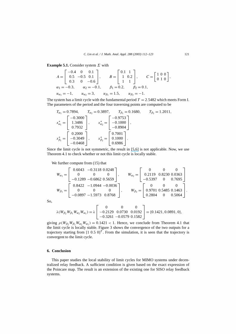
Fig. 1. Decentralized relay feedback systems.

Define the switching planes

Sαi := {ξ ∈ Rn: ciξ = αi}, Sβi := {ξ ∈ R

n: ciξ = βi}, i = 1,2, . . . ,m. (4)

Let

S+αi

:= {ξ ∈ Rn: ciξ > αi}, S−

αi:= {ξ ∈ R

n: ciξ < αi}, i = 1,2, . . . ,m, (5)

and letS+βi

andS−βi

be defined similarly. For a certaini = 1,2, . . . ,m, if a trajectory of

systemΣ , evolving fromS+βi

(respectively,S−αi

), traversesSαi (respectively,Sβi ) atx, thenwe will call the statex a traversing point. The time instant corresponding to the traverspoint is calledswitching instant. It should be stressed that in our convention forαi < βi , ifa trajectory traversesSαi atx fromS−

αi(respectively, traversesSβi atx fromS+

βi), the state

x is not called a traversing point, since such traversing does not cause a switch inu(t).In this note, we will study the local stability of a certain type of limit cycles. The lo

stability means that all nearby trajectories converge to the limit cycle as time teninfinity. A sufficient condition is given in terms of the spectral radius of a construmatrix.

3. Determination of limit cycles

The starting point in the analysis is to assume that a limit cycle exists in systemΣ . Asin [5,6], we assume that the outputs from all the relays under the limit cycle are swaves with the same fundamental period, but with different phase shifts. Without logenerality, assume that them relays switch in the sequence ofu1, u2, . . . , um. In a moredetail, the considered limit cycle is of the following form.

Form I. Each relay under the limit cycle switches two times within a fundamental peThe fundamental period isT = ∑m

i=1Tαi +∑mi=1Tβi , whereTαi andTβi , i = 1,2, . . . ,

m−1, are, respectively, the time durations for the trajectory of the limit cycle to movethe traversing pointx∗

αi∈ Sαi to the successive onex∗

αi+1∈ Sαi+1 and from the traversin

pointx∗βi

∈ Sβi to the successive onex∗βi+1

∈ Sβi+1, andTαm andTβm are, respectively, fromx∗α to x∗ and fromx∗ to x∗

α .

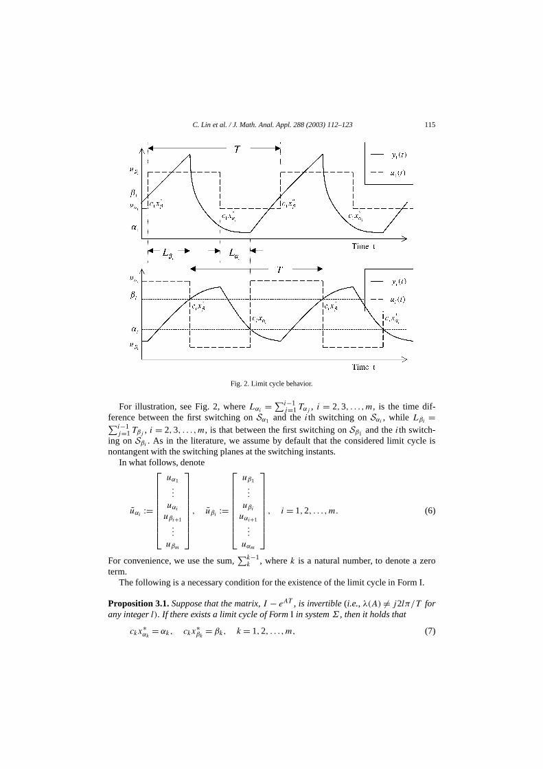
C. Lin et al. / J. Math. Anal. Appl. 288 (2003) 112–123 115

le is

ro

I.

Fig. 2. Limit cycle behavior.

For illustration, see Fig. 2, whereLαi = ∑i−1j=1Tαj , i = 2,3, . . . ,m, is the time dif-

ference between the first switching onSα1 and theith switching onSαi , while Lβi =∑i−1j=1Tβj , i = 2,3, . . . ,m, is that between the first switching onSβ1 and theith switch-

ing onSβi . As in the literature, we assume by default that the considered limit cycnontangent with the switching planes at the switching instants.

In what follows, denote

uαi :=

uα1...

uαiuβi+1...

uβm

, uβi :=

uβ1...

uβiuαi+1...

uαm

, i = 1,2, . . . ,m. (6)

For convenience, we use the sum,∑k−1

k , wherek is a natural number, to denote a zeterm.

The following is a necessary condition for the existence of the limit cycle in Form

Proposition 3.1. Suppose that the matrix, I − eAT , is invertible (i.e., λ(A) = j2lπ/T forany integer l). If there exists a limit cycle of Form I in system Σ , then it holds that

ckx∗α = αk, ckx

∗β = βk, k = 1,2, . . . ,m, (7)

k k

116 C. Lin et al. / J. Math. Anal. Appl. 288 (2003) 112–123

where

x∗αk

= (I − eAT )−1

(m∑j=k

Tβj∫0

eA(∑k−1

i=1 Tαi+∑m

i=j Tβi−s)Buβj ds

+k−1∑j=1

Tαj∫0

eA(∑k−1

i=j Tαi−s)Buαj ds

+m∑j=k

Tαj∫0

eA(∑m

i=1 Tβi+∑k−1

i=1 Tαi+∑m

i=j Tαi−s)Buαj ds

+k−1∑j=1

Tβj∫0

eA(∑k−1

i=1 Tαi+∑m

i=j Tβi−s)Buβj ds), (8)

x∗βk

= (I − eAT )−1

(m∑j=k

Tαj∫0

eA(∑k−1

i=1 Tβi+∑m

i=j Tαi−s)Buαj ds

+k−1∑j=1

Tβj∫0

eA(∑k−1

i=j Tβi−s)Buβj ds

+m∑j=k

Tβj∫0

eA(∑m

i=1 Tαi+∑k−1

i=1 Tβi+∑m

i=j Tβi−s)Buβj ds

+k−1∑j=1

Tαj∫0

eA(∑k−1

i=1 Tβi+∑m

i=j Tαi−s)Buαj ds). (9)

Proof. If there exists a limit cycle of Form I, it should satisfy

ckx∗αk

= αk, ckx∗βk

= βk, k = 1,2, . . . ,m, (10)

and

x∗α1

= eATβm x∗βm

+Tβm∫0

eA(Tβm−s)Buβm ds,

x∗αk

= eATαk−1x∗

αk−1+

Tαk−1∫eA(Tαk−1−s)

Buαk−1 ds, k = 2, . . . ,m,

0

C. Lin et al. / J. Math. Anal. Appl. 288 (2003) 112–123 117

nda-thetainedO one2.1

x∗β1

= eATαm x∗αm

+Tαm∫0

eA(Tαm−s)Buαm ds,

x∗βk

= eATβk−1x∗

βk−1+

Tβk−1∫0

eA(Tβk−1−s)

Buβk−1 ds, k = 2, . . . ,m. (11)

From (11), we obtain fork = 1,2, . . . ,m that

x∗αk

= eA(∑k−1

i=1 Tαi+∑m

i=k Tβi )x∗βk

+m∑j=k

Tβj∫0

eA(∑k−1

i=1 Tαi+∑m

i=j Tβi−s)Buβj ds

+k−1∑j=1

Tαj∫0

eA(∑k−1

i=j Tαi−s)Buαj ds, (12)

x∗βk

= eA(∑k−1

i=1 Tβi+∑m

i=k Tαi )x∗αk

+m∑j=k

Tαj∫0

eA(∑k−1

i=1 Tβi+∑m

i=j Tαi−s)Buαj ds

+k−1∑j=1

Tβj∫0

eA(∑k−1

i=j Tβi−s)Buβj ds. (13)

Note thatT =∑mi=1Tαi +∑m

i=1Tβi . Left multiplying (13) byeA(∑k−1

i=1 Tαi+∑m

i=k Tβi ) and

combining with (12) yield (8) while left multiplying (12) byeA(∑k−1

i=1 Tβi+∑m

i=k Tαi ) andcombining with (13) yield (9). This proves the proposition.✷Remark 3.1. Equation (7) gives a closed form for solving the parameters of the fumental period,Tαi andTβi , i = 1,2, . . . ,m. Numerical procedure has to be used. Oncesolutions correspond to a limit cycle, the parameters of the traversing points are obas in (8) and (9). It is easy to see that for the special case when the system is SIS(m= 1) with α1 + β1 = 0, Proposition 3.1 reduces to Theorem 5.1 in [1] or Theoremin [1] for symmetric limit cycle anduα1 + uβ1 = 0.

4. Criterion for local stability of limit cycles

The main result in this section is as follows.

Theorem 4.1. Suppose there exists a limit cycle of Form I in system Σ . Then the limit cycleis locally stable if

ρ

(m∏Wβj

m∏Wαi

)< 1, (14)

j=1 i=1

118 C. Lin et al. / J. Math. Anal. Appl. 288 (2003) 112–123

t

y

where ρ(·) denotes the spectral radius of a matrix, and

Wαi =(I − (Ax∗

αi+1+Buαi )ci+1

ci+1(Ax∗αi+1

+Buαi )

)eATαi , i = 1,2, . . . ,m− 1,

Wαm =(I − (Ax∗

β1+Buαm)c1

c1(Ax∗β1

+Buαm)

)eATαm ,

Wβj =(I −

(Ax∗βj+1

+Buβj )cj+1

cj+1(Ax∗βj+1

+Buβj )

)eATβj , j = 1,2, . . . ,m− 1,

Wβm =(I − (Ax∗

α1+Buβm)c1

c1(Ax∗α1

+Buβm)

)eATβm . (15)

Proof. Consider the limit cycle in Form I. Without loss of generality, we lett0 = 0 cor-respond to the time instant when the relay switch fromuβm−1 to uβm . This means thathe initial point of the limit cycle is chosen to bex∗

0 = x∗βm

and it holds thatcix∗0 > αi ,

i = 1,2, . . . ,m. Let

ε0 := mini

{(cix

∗0 − αi

)‖ci‖−1}. (16)

Define theε-neighborhood aroundx∗0 as

Rε := {ξ ∈ Rn:

∥∥ξ − x∗0

∥∥< ε}= {

ξ ∈Rn: ξ = x∗0 +(, ( ∈ Rn, ‖(‖< ε

}. (17)

Then, any trajectory of systemΣ starting atx0 = x∗0 +( ∈ Rε0 can evolve withu(0)=

uβm . This is becausecix0 = ci(x∗0 +()> αi , i = 1,2, . . . ,m, for ‖(‖< ε0.

We now analyze the trajectory ofx(t) starting from a nearby point tox∗0. By continuity,

if ε (� ε0) is small enough, then any trajectory starting fromx0 ∈ Rε will traverseSα1 at

a certain pointx(1)α1 . Moreover,‖x(1)α1 − x∗α1

‖ can be made arbitrarily small by choosingε,and thus‖x0 − x∗

0‖, sufficiently small. With a similar way, by choosingx0 close enoughto x∗

0, the trajectory starting fromx0 will evolve close to the limit cycle (while the relaswitches for the second, third,. . . , (2m+ 1)th time) and return to traverseSα1 at another

point x(2)α1 . The Poincare mapP :Rε ∩ Sα1 → Sα1 is defined asP(x(1)α1 )= x(2)α1 . Next, we

compute the exact expression ofP by relatingx(2)α1 − x∗α1

to x(1)α1 − x∗α1

.

Let the trajectory ofx(t) spend a time durationTα1 + δ(1)α1 from x

(1)α1 ∈ Sα1 to traverse

Sα2 at x(1)α2 . Then,

x(1)α2= eA(Tα1+δ(1)α1 )x(1)α1

+Tα1+δ(1)α1∫

0

eA(Tα1+δ(1)α1 −s)Buα1 ds,

c2x(1)α2

= α2. (18)

Taking into account

C. Lin et al. / J. Math. Anal. Appl. 288 (2003) 112–123 119

o

s

x∗α2

= eATα1x∗α1

+Tα1∫0

eA(Tα1−s)Buα1 ds,

c2x∗α2

= α2, (19)

after some manipulations, we have

c2eA(Tα1+δ(1)α1 )

(x(1)α1

− x∗α1

)+ c2(eAδ

(1)α1 − I

)x∗α2

+ c2

δ(1)α1∫

0

eAsBuα1 ds = 0. (20)

For t ∈ R, define

fα1(t) := c2(eAt − I)x∗

α2+ c2

t∫0

eAsBuα1 ds.

Then,

t−1fα1(t)→ c2Ax∗α2

+ c2Buα1 < 0 ast → 0.

By defining

t−1fα1(t)∣∣t=0 := lim

t→0t−1fα1(t),

there exists a scalarrα1 > 0 such thatt−1fα1(t) < 0 is continuous ont ∈ [−rα1, rα1]. So,

δ(1)α1 f

−1α1(δ(1)α1 ) is well defined by choosing smallε such that|δ(1)α1 | � rα1. This enables us t

get from (20) that

δ(1)α1= −δ(1)α1

f−1α1

(δ(1)α1

)c2e

A(Tα1+δ(1)α1 )(x(1)α1

− x∗α1

). (21)

Using (18), (19) and (21), after simple deductions, we obtain

x(1)α2− x∗

α2= eA(Tα1+δ(1)α1 )

(x(1)α1

− x∗α1

)+ (eAδ(1)α1 − I)x∗

α2+ ∫ δ(1)α1

0 eAsBuα1 ds

δ(1)α1

δ(1)α1

=(I − ((eAδ

(1)α1 − I)x∗

α2+ ∫ δ(1)α1

0 eAsBuα1 ds)c2

c2((eAδ

(1)α1 − I)x∗

α2+ ∫ δ(1)α1

0 eAsBuα1 ds)

)

× eA(Tα1+δ(1)α1 )(x(1)α1

− x∗α1

). (22)

The above shows the relation betweenx(1)α2 − x∗

α2andx(1)α1 − x∗

α1. Similar deduction lead

to the relation betweenx(2)α1 − x∗α1

andx(1)α1 − x∗α1

, given by

x(2)α1− x∗

α1=(

m∏j=1

Wβj

(δ(1)βj

) m∏i=1

Wαi

(δ(1)αi

))(x(1)α1

− x∗α1

), (23)

where

120 C. Lin et al. / J. Math. Anal. Appl. 288 (2003) 112–123

he

theyg

s

ycle

th syn-rion incles

Wαi

(δ(1)αi

)=(I − ((eAδ

(1)αi − I)x∗

αi+1+ ∫ δ(1)αi

0 eAsBuαi ds)ci+1

ci+1((eAδ

(1)αi − I)x∗

αi+1+ ∫ δ(1)αi

0 eAsBuαi ds)

)eA(Tαi+δ

(1)αi),

i = 1,2, . . . ,m− 1,

Wαm

(δ(1)αm

)=(I − ((eAδ

(1)αm − I)x∗

β1+ ∫ δ(1)αm

0 eAsBuαm ds)c1

c1((eAδ

(1)αm − I)x∗

β1+ ∫ δ(1)αm

0 eAsBuαm ds)

)eA(Tαm+δ(1)αm ),

Wβj

(δ(1)βj

)=(I −

((eAδ

(1)βj − I)x∗

βj+1+ ∫ δ(1)βj

0 eAsBuβj ds)cj+1

cj+1((eAδ

(1)βj − I)x∗

βj+1+ ∫ δ(1)βj

0 eAsBuβj ds)

)eA(Tβj +δ(1)βj

),

j = 1,2, . . . ,m− 1,

Wβm

(δ(1)βm

)=(I − ((e

Aδ(1)βm − I)x∗

α1+ ∫ δ(1)βm

0 eAsBuβm ds)c1

c1((eAδ

(1)βm − I)x∗

α1+ ∫ δ(1)βm

0 eAsBuβm ds)

)eA(Tβm+δ(1)βm

). (24)

Furthermore, all the time differences,δ(1)αk andδ(1)βk, k = 1,2, . . . ,m (of the time durations

for the two trajectories ofx(t) and the limit cycle to move from a traversing point to tsuccessive one), can be arbitrarily close to zero by choosingε sufficiently small.

Now, letting δ(1)αk → 0 andδ(1)βk→ 0, we see thatWαk (δ

(1)αk ) → Wαk andWβk (δ

(1)βk) →

Wβk , k = 1,2, . . . ,m. From theory of discrete-time systems, it can be shown that ifcondition in (14) is satisfied, then there exists a scalarε (� ε0) such that any trajectorstarting fromRε will traverseSα1 consecutively. Moreover, thelth returned traversin

point,x(l+1)α1 , which relates to its former onex(l)α1 by a formula similar to that in (23), tend

to x∗α1

as the natural numberl increases. This completes the proof of the theorem.✷Remark 4.1. The matrices in (15) satisfy thatc1Wαm = ci+1Wαi = c1Wβm = cj+1Wβj = 0for i, j = 1,2, . . . ,m− 1. So, the matrix in (14) always has a zero eigenvalue.

Remark 4.2. For the special case when the system is SISO one (m= 1) with α1 + β1 = 0,Theorem 4.1 reduces to Theorem 5.2 in [1] or Theorem 3.1 in [1] for symmetric limit canduα1 + uβ1 = 0.

Remark 4.3. The method in [5,6] is frequency-domain based and uses theZ-transformtechnique to convert the system to an equivalent fictitious sampled-data system wichronous samplers, while our analysis is state-space based and the stability criteTheorem 4.1 is easy to apply. Moreover, the result in [5,6] is for symmetric limit cyonly while our result is also applicable to asymmetric limit cycles.

5. A numerical example

In this section, we give a numerical example to illustrate the use of our results.

C. Lin et al. / J. Math. Anal. Appl. 288 (2003) 112–123 121

I.

use

hatfor ais

cen-ion ofdback

Example 5.1. Consider systemΣ with

A=−0.4 0 0.1

0.5 −0.5 0.10.3 0 −0.6

, B =

0.1 1

1 0.21 1

, C =

[1 0 00 1 0

],

α1 = −0.3, α2 = −0.1, β1 = 0.2, β2 = 0.1,

uα1 = −1, uα2 = 3, uβ1 = 1.5, uβ2 = −1.

The system has a limit cycle with the fundamental periodT = 2.5482 which meets FormThe parameters of the period and the four traversing points are computed to be

Tα1 = 0.7894, Tα2 = 0.3897, Tβ1 = 0.1680, Tβ2 = 1.2011,

x∗α1

=−0.3000

1.34860.7932

, x∗

α2=−0.9753

−0.1000−0.8904

,

x∗β1

= 0.2000

−0.3049−0.0468

, x∗

β2= 0.7001

0.10000.6986

.

Since the limit cycle is not symmetric, the result in [5,6] is not applicable. Now, weTheorem 4.1 to check whether or not this limit cycle is locally stable.

We further compute from (15) that

Wα1 = 0.6043 −0.3118 0.0248

0 0 0−0.1289 −0.6862 0.5659

, Wα2 =

0 0 0

0.2119 0.8230 0.0363−0.5397 0 0.7695

Wβ1 = 0.8422 −1.0944 −0.0036

0 0 0−0.0897−1.5973 0.8768

, Wβ2 =

0 0 0

0.9701 0.5485 0.14630.2804 0 0.5064

.

So,

λ(Wβ2Wβ1Wα2Wα1)= λ

0 0 0

−0.2129 0.0730 0.0192−0.3261−0.0579 0.1582

= {0.1421,0.0891,0},

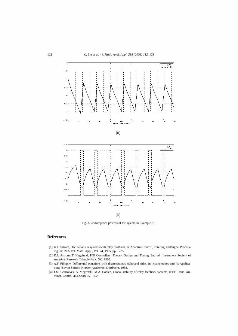
giving ρ(Wβ2Wβ1Wα2Wα1) = 0.1421< 1. Hence, we conclude from Theorem 4.1 tthe limit cycle is locally stable. Figure 3 shows the convergence of the two outputstrajectory starting from[1 0.5 0]T . From the simulation, it is seen that the trajectoryconvergent to the limit cycle.

6. Conclusion

This paper studies the local stability of limit cycles for MIMO systems under detralized relay feedback. A sufficient condition is given based on the exact expressthe Poincare map. The result is an extension of the existing one for SISO relay feesystems.

122 C. Lin et al. / J. Math. Anal. Appl. 288 (2003) 112–123

cess-

ety of

plica-

. Au-

Fig. 3. Convergence process of the system in Example 5.1.

References

[1] K.J. Astrom, Oscillations in systems with relay feedback, in: Adaptive Control, Filtering, and Signal Proing, in: IMA Vol. Math. Appl., Vol. 74, 1995, pp. 1–25.

[2] K.J. Astrom, T. Hagglund, PID Controllers: Theory, Design and Tuning, 2nd ed., Instrument SociAmerica, Research Triangle Park, NC, 1995.

[3] A.F. Filippov, Differential equations with discontinuous righthand sides, in: Mathematics and Its Aptions (Soviet Series), Kluwer Academic, Dordrecht, 1988.

[4] J.M. Goncalves, A. Megretski, M.A. Dahleh, Global stability of relay feedback systems, IEEE Transtomat. Control 46 (2000) 550–562.

C. Lin et al. / J. Math. Anal. Appl. 288 (2003) 112–123 123

1992)

lized

relay

relay

[5] Z.J. Palmor, Y. Halevi, T. Efrati, Limit cycles in decentralized relay systems, Internat. J. Control 56 (755–765.

[6] Z.J. Palmor, Y. Halevi, T. Efrati, A general and exact method for determining limit cycles in decentrarelay systems, Automatica 31 (1995) 1333–1339.

[7] Z.Ya. Tsypkin, Relay Control Systems, Cambridge Univ. Press, New York, 1984.[8] Q.-G. Wang, B. Zou, T.-H. Lee, Q. Bi, Auto-tuning of multivariable PID controllers from decentralized

feedback, Automatica 33 (1997) 319–330.[9] Q.-G. Wang, C.-C. Hang, B. Zou, Multivariable process identification and control from decentralized

feedback, Internat. J. Modelling Simulation 20 (2000) 341–348.[10] C.C. Yu, Autotuning of PID Controllers, Springer, London, 1999.