LISFLOOD: a GIS-based distributed model for river basin scale water balance and flood simulation

Research Article

LISFLOOD: a GIS-based distributed model for river basin scale waterbalance and flood simulation

J. M. VAN DER KNIJFF, J. YOUNIS and A. P. J. DE ROO*

Land Management & Natural Hazards Unit, Institute for Environment and

Sustainability, DG Joint Research Centre, European Commission, Italy

(Received 30 July; in final form 13 September 2008)

In this paper we describe the spatially distributed LISFLOOD model, which is a

hydrological model specifically developed for the simulation of hydrological

processes in large European river basins. The model was designed to make the

best possible use of existing data sets on soils, land cover, topography and

meteorology. We give a detailed description of the simulation of hydrological

processes in LISFLOOD, and discuss how the model is parameterized. We also

describe how the model was implemented technically using a combination of the

PCRaster GIS system and the Python programming language, and discuss the

management of in- and output data. Finally, we review some recent applications

of LISFLOOD, and we present a case study for the Elbe river.

Keywords: LISFLOOD; PCRaster; Rainfall-runoff models; Floods

1. Introduction

LISFLOOD is a GIS-based hydrological rainfall-runoff-routing model that is capable

of simulating the hydrological processes that occur in a catchment. The specific

development objective was to produce a tool that can be used in large and trans-

national catchments for a variety of applications, including flood forecasting, and

assessing the effects of river regulation measures, land-use change and climate change.

Although a wide variety of existing hydrological models are available that are suitable

for each of these individual tasks, few single models are capable of doing all these

jobs. For example, the Swedish HBV hydrology model (Hydrologiska Byrans

Vattenbalansmodel) (e.g. Lindstrom et al. 1997) is a rainfall-runoff model with

appropriate process descriptions for our needs, but it lacks a spatially distributed river

routing component. MIKE-SHE (DHI 2000) is a very good physically-based model,

but it cannot be used for larger river basins. MIKE-11 (Havnø et al. 1995) is better

suited in this respect, but its rainfall-runoff component is not quite sophisticated

enough for our purposes. HEC-RAS (Brunner 2008) is limited to river routing only

and does not contain a rainfall-runoff component at all. TOPKAPI (Ciarapica and

Todini 2002) is a river basin model that extends the classic TOPMODEL (Beven and

Kirkby 1979) approach. Its current range of application fields shows some overlap

with LISFLOOD; however, TOPKAPI was applied to and tested for smaller river

basins only when the development of LISFLOOD started. The American HEC-HMS

(Scharffenberg and Fleming 2008) is a semi-lumped model.

*Corresponding author. Email: [email protected]

International Journal of Geographical Information Science

Vol. 24, No. 2, February 2010, 189–212

International Journal of Geographical Information ScienceISSN 1365-8816 print/ISSN 1362-3087 online # 2010 Taylor & Francis

http://www.tandf.co.uk/journalsDOI: 10.1080/13658810802549154

Downloaded By: [De Roo, A. P. J.][Commission European Comm] At: 16:50 1 March 2010

Our objective requires a model that is spatially distributed and—at least to a

certain extent—physically-based. Also, the focus of our work is on European

catchments. Since several (spatial) databases exist that contain pan-European

information on soils (King et al. 1997, Wosten et al. 1999), land cover (CEC 1993),

topography (Hiederer and de Roo 2003) and meteorology (Rijks et al. 1998), it

would be advantageous to have a model that makes the best possible use of these

data. Finally, the wide scope of our objective implies that changes and extensions to

the model will be required from time to time. Therefore, it is essential to have a

model code that can be easily maintained and modified. LISFLOOD has been

specifically developed to satisfy these requirements. In parallel to LISFLOOD, a

separate flood inundation model called LISFLOOD-FP has been developed as well

(Bates and de Roo 2000). To avoid any confusion, we would like to stress that both

are different (although complementary) models. LISFLOOD-FP will not be

discussed in this paper.

Some examples of recent applications of LISFLOOD are given in Feyen et al.

(2007), Feyen et al. (2008), Gouweleeuw et al. (2004), Dankers et al. (2007), Thielen

et al. (2008) and Younis et al. (2008a, b). These papers include a brief description of

the model only. A paper by de Roo et al. (2000) describes an earlier version of the

model. Considerable changes have been incorporated into the model since that

paper was published. The aim of the current paper is to provide an up-to-date

description that reflects the current state of the model. We do this by first outlining

in section 2 the general characteristics of the model, followed by a description of the

individual processes that are included. In section 3 we provide an overview of the

methods and data sources that are used to parameterize the model. In section 4 we

explain how we implemented the model using a combination of the PCRaster

Dynamic Modelling language (Wesseling et al. 1996, Karssenberg 2002) and the

Python scripting language (Python 2008). We also explain here why we decided on

such an approach. Section 5 discusses the management of LISFLOOD’s in- and

output data. Finally, in section 6 we give an overview of some recent applications of

the model, and present a new case study. We end with a concluding section.

2. Simulation of hydrological processes

LISFLOOD is a spatially distributed, grid-based rainfall-runoff and channel routing

model. It can run using any desired time interval, on any grid size. The model is

typically run using a daily time interval to simulate the long-term catchment water

balance, whereas smaller intervals (e.g. hourly) are better suited to modelling

individual flood events. Both can be combined as well. For instance, the state

variables at the end of a (daily) water balance run can be used to provide the initial

conditions for an (hourly) flood run. The model does not impose any limitations on

the grid resolution that is used. However, its separation between runoff-generating

and channel routing processes would be poorly represented at very low pixel

resolutions. Since LISFLOOD has been primarily developed for the simulation of

large river basins, small-scale processes are often simulated in a simplified way.

Because of this, there would be little benefit in using very high resolutions either. We

would therefore recommend using the model at grid resolutions within the range of

100–10 km. Most current applications of the model have employed grid resolutions

of 1 or 5 km. Figure 1 gives an overview of the structure of LISFLOOD. As the

figure shows, the model is made up of a two-layer soil water balance sub-model, sub-

models for the simulation of groundwater and subsurface flow (using two parallel

190 J.M. van der Knijff et al.


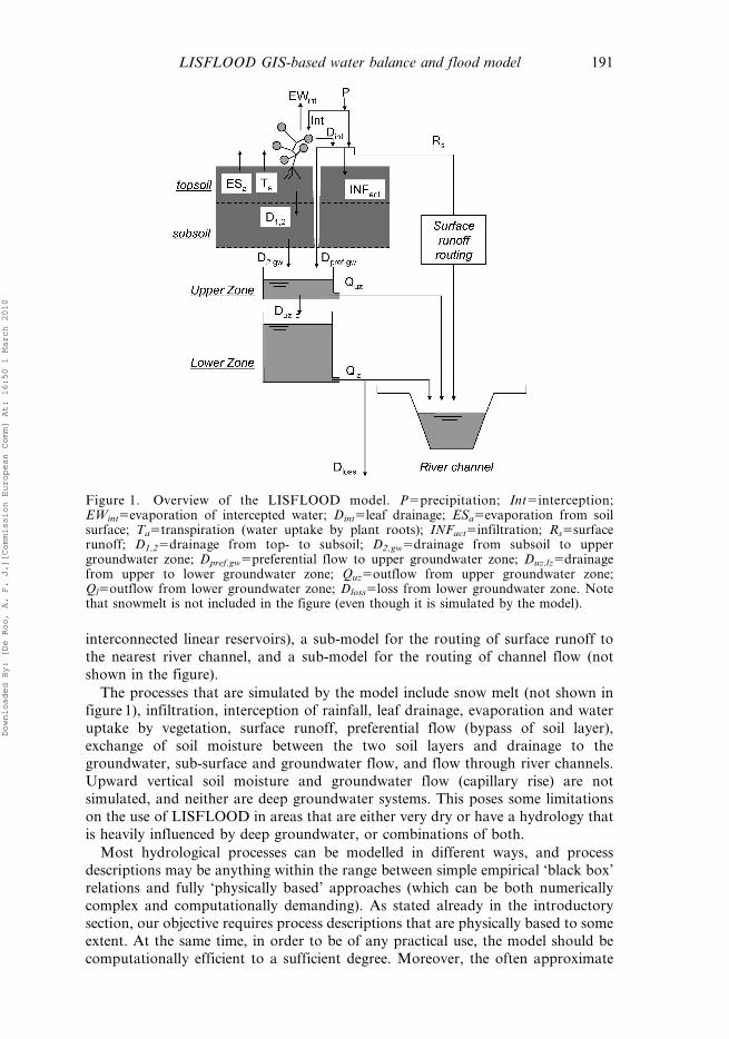
interconnected linear reservoirs), a sub-model for the routing of surface runoff to

the nearest river channel, and a sub-model for the routing of channel flow (not

shown in the figure).

The processes that are simulated by the model include snow melt (not shown in

figure 1), infiltration, interception of rainfall, leaf drainage, evaporation and water

uptake by vegetation, surface runoff, preferential flow (bypass of soil layer),

exchange of soil moisture between the two soil layers and drainage to thegroundwater, sub-surface and groundwater flow, and flow through river channels.

Upward vertical soil moisture and groundwater flow (capillary rise) are not

simulated, and neither are deep groundwater systems. This poses some limitations

on the use of LISFLOOD in areas that are either very dry or have a hydrology that

is heavily influenced by deep groundwater, or combinations of both.

Most hydrological processes can be modelled in different ways, and process

descriptions may be anything within the range between simple empirical ‘black box’

relations and fully ‘physically based’ approaches (which can be both numerically

complex and computationally demanding). As stated already in the introductorysection, our objective requires process descriptions that are physically based to some

extent. At the same time, in order to be of any practical use, the model should be

computationally efficient to a sufficient degree. Moreover, the often approximate

Figure 1. Overview of the LISFLOOD model. P5precipitation; Int5interception;EWint5evaporation of intercepted water; Dint5leaf drainage; ESa5evaporation from soilsurface; Ta5transpiration (water uptake by plant roots); INFact5infiltration; Rs5surfacerunoff; D1,25drainage from top- to subsoil; D2,gw5drainage from subsoil to uppergroundwater zone; Dpref,gw5preferential flow to upper groundwater zone; Duz,lz5drainagefrom upper to lower groundwater zone; Quz5outflow from upper groundwater zone;Ql5outflow from lower groundwater zone; Dloss5loss from lower groundwater zone. Notethat snowmelt is not included in the figure (even though it is simulated by the model).

LISFLOOD GIS-based water balance and flood model 191


nature of data derived from large-scale datasets—such as the pan-European

databases mentioned in the introduction—would not support an approach that is

fully physically based. Finally, limitations of the more physically based approaches

have been discussed at length in the more recent literature (see e.g. Beven 2001 for an

overview). For LISFLOOD we have aimed to select process descriptions that make

the best use of available prior data – thus reducing the number of calibration

parameters, but we have tried to avoid process descriptions that are overly complex,

computationally demanding or irrelevant at the scale of large catchments. In the

following we describe the individual processes in more detail.

2.1 Meteorological forcing

LISFLOOD is driven by the following meteorological variables: precipitation

intensity, P (mm day21), potential (reference) evapotranspiration rate of a closed

canopy, ET0 (mm day21), potential (reference) evaporation rate from a bare soil

surface, ES0 (mm day21), potential evaporation rate from an open water surface,

EW0 (mm day21), and average 24-hour temperature, Tavg (uC). ET0, ES0 and EW0

are all calculated outside the model, and a separate pre-processing application that

calculates these variables from standard meteorological observations is available as

a companion to the model. LISFLOOD always expects these input variables in the

units as given above, irrespective of the actual time step used. In other words: even if

the model is run on an hourly time step, precipitation must be provided as an

intensity with units (mm day21). Note that in the remainder of the description that

follows, all rate variables are expressed in (mm) per time step, unless stated

otherwise.

2.2 Snow and frost

If the average daily temperature is below 1uC, all precipitation is assumed to be

snow. A snow correction factor can be applied to correct for undercatch of snow

precipitation. Unlike rain, snow accumulates on the soil surface until it melts. Rates

of snowmelt can be estimated by simulating the full surface radiation balance.

However, a comparative study of different snowmelt models by the World

Meteorological Organization did not demonstrate such models to be superior to

much simpler modelling approaches that are based on temperature indices (WMO

1986). Since radiation balance models are rather data-demanding (both in terms of

parameters that need to be estimated as well in meteorological input data),

LISFLOOD uses the following simple degree-day factor equation instead (Speers

et al. 1979, cited in Young 1985):

M~Cm 1z0:01:RDtð Þ Tavg{Tm

� �:Dt ð1Þ

where M is the rate of snowmelt (mm), Cm is a degree-day factor (mm uC21 day21),

R is the rainfall intensity (mm day21), Dt is the time interval (days), Tavg is the

average 24-hour temperature (uC), and Tm is the temperature above which snowmelt

occurs (uC). The equation takes into account accelerated snowmelt when it is

raining. For large pixel sizes, there may be considerable sub-pixel heterogeneity in

snow accumulation and melt, which is a particular problem if there are large

elevation differences within a pixel. Because of this, melt and accumulation of snow

are modelled separately for three separate elevation zones, which are defined at the

sub-pixel level.



When the soil is frozen, this affects the hydrological processes occurring near its

surface. In LISFLOOD it is assumed that evaporation from the soil surface, water

uptake by vegetation, infiltration, and flow of moisture through the soil matrix are

all reduced to zero. To establish whether the soil surface is frozen or not, a frost

index F is calculated (re-written from Molnau and Bissell 1983, cited in Maidment

1993):

F tð Þ~F t{1ð Þ{ 1{Af

� �FDt{Tavg

:e{0:04:K :ds=wesDt ð2Þ

where F is expressed in (uC day21). Af is a decay coefficient (day21), K is a snow

depth reduction coefficient (cm21), ds is the depth of the snow cover (expressed as an

equivalent water depth (mm)), and wes is the equivalent water depth of a given depth

of snow cover. The soil is considered frozen if F is above a critical threshold Fcrit; F is

always greater than or equal to 0.

2.3 Interception

Interception of rainfall is often simulated using some variation on the classic Rutter

model (e.g. Rutter et al. 1971, Gash 1979). Since it is very difficult to obtain reliable

estimates of interception-related vegetation characteristics at the continental scale,

LISFLOOD follows the even simpler approach of Aston (1979) and Merriam

(1960), which requires only two parameters. Interception is estimated as:

Int~Smax: 1{exp {k:RDt=Smaxð Þ½ � ð3Þ

where Int (mm) is the interception per time step, Smax (mm) is the maximum

interception, R is the rainfall intensity (mm day21) and the factor k accounts for the

density of the vegetation. Smax is calculated using the empirical relation (von

Hoyningen-Huene 1981):

Smax~0:935z0:498LAI{0:00575LAI2 LAIw0:1ð ÞSmax~0 LAIƒ0:1ð Þ

(

ð4Þ

where LAI is the average Leaf Area Index (m2 m22) of each grid cell. Constant k is

given by:

k~0:046LAI ð5Þ

The value of Int can never exceed the interception storage capacity, which is defined

as the difference between Smax and the accumulated amount of water that is stored

as interception, Intcum. Evaporation of intercepted water, EWint, occurs at the

potential evaporation rate from an open water surface, EW0. The maximum

evaporation per time step is proportional to the fraction of vegetated area in each

pixel (Supit et al. 1994):

EWmax~EW0: 1{exp {kgb:LAI

� �� Dt ð6Þ

where EW0 is the potential evaporation rate from an open water surface

(mm day21), and EWmax is in (mm) per time step. Constant kgb is the extinction

coefficient for global solar radiation. Since evaporation is limited by the amount of

water stored on the leaves, the actual amount of evaporation from the interception

store equals (Supit et al. 1994):



EWint~min EWmaxDt, Intcumð Þ ð7Þ

where EWint is the actual evaporation from the interception store in (mm) per time

step, and EW0 is the potential evaporation rate from an open water surface

(mm day21). It is assumed that on average all water in the interception store (Intcum)

will have evaporated or fallen to the soil surface as leaf drainage within one day.

Leaf drainage is therefore modelled as a linear reservoir with a time constant of one

day:

Dint~1

Tint

:IntcumDt ð8Þ

where Dint is the amount of leaf drainage per time step (mm) and Tint is a time

constant for the interception store (days), which is set to one day.

2.4 Treatment of impervious areas

If (part of) a pixel is made up of built-up area this will influence that pixel’s water-

balance. The ‘direct runoff fraction’ parameter (fdr) defines the fraction of a pixel

that is impervious. For impervious areas, it is assumed that:

(i) any water that reaches the surface is added directly to surface runoff;

(ii) the storage capacity of the soil is zero (i.e. no soil moisture storage in the

direct runoff fraction);

(iii) there is no groundwater storage.

The same assumptions are made for open water bodies (e.g. lakes), which are

included in fdr. Unless stated otherwise, the description of all subsurface processes

below (evaporation, transpiration, infiltration, preferential flow, soil moisture

redistribution and groundwater flow) are valid for the pervious domain of each pixel

(i.e. 12fdr) only. In the pervious fraction of each pixel (12fdr), the amount of water

that is available for infiltration, Wav (mm) equals:

Wav~RDtzMzDint{Int ð9Þ

where R is the rainfall intensity (mm day21), and M, Dint and Int are the amounts of

snowmelt, leaf drainage and interception, respectively (all in (mm) per time step).

Since no infiltration can take place in each pixel’s ‘direct runoff fraction’, direct

runoff is calculated as:

Rd~fdrWav ð10Þ

with Rd is in (mm) per time step. Note here that Wav is valid for the pervious fraction

only, whereas Rd is valid for the direct runoff fraction.

2.5 Evapotranspiration

Water uptake and transpiration by vegetation and direct evaporation from the soil

surface are modelled as two separate processes. Our approach is largely based on

Supit et al. (1994) and Supit and van der Goot (2003), which is in turn an adaptation

of the widely used FAO Penman-Monteith method (Allen et al. 1998). The main

reason for using this method is that it is a widely accepted approach. Moreover, it

uses meteorological forcing variables that are identical to the ones stored in an



existing pan-European agro-meteorological database (Rijks et al. 1998). This means

that the historical data in the database can be used directly as input to LISFLOOD.

The maximum transpiration per time step (mm) is calculated as:

Tmax~kcrop:ET0: 1{exp {kgb

:LAI� ��

Dt{EWint ð11Þ

where ET0 is the potential (reference) evapotranspiration rate (mm day21), and kcrop

is a crop coefficient. Note that the energy that has been ‘consumed’ already for the

evaporation of intercepted water is simply subtracted here in order to respect the

overall energy balance. The actual transpiration rate is reduced in case of water

stress. A reduction factor is applied to account for this:

rws~w1{wwp1

wcrit1{wwp1ð12Þ

where w1 is the amount of moisture in the upper soil layer (mm), wwp1 (mm) is the

amount of soil moisture at wilting point (pF 4.2) and wcrit1 (mm) is the amount of

moisture below which water uptake is reduced and plants start closing their stomata.

The critical amount of soil moisture is calculated as:

wcrit1~ 1{pð Þ: wfc1{wwp1

� �zwwp1 ð13Þ

where wfc1 (mm) is the amount of soil moisture at field capacity and p is the soil

water depletion fraction. Parameter p represents the fraction of soil moisture

between wfc1 and wwp1 that can be extracted from the soil without reducing the

transpiration rate, and its value is a function of both ET0 and land cover (details on

this can be found in Supit and Van Der Goot (2003)). Reduction factor rWS is

allowed to assume values between 0 and 1 only. The actual transpiration Ta is now

calculated as:

Ta~rws:Tmax ð14Þ

with both Ta and Tmax in (mm).

The maximum amount of evaporation from the soil surface equals the maximum

evaporation from a shaded soil surface, ESmax (mm), which is computed as:

ESmax~ES0 exp {kgbLAI� �

Dt ð15Þ

where ES0 is the potential evaporation rate from bare soil surface (mm day21). The

actual evaporation from the soil mainly depends on the amount of soil moisture

near the soil surface: evaporation decreases as the topsoil dries out. This is simulated

using a reduction factor which is a function of the number of days since the last rain

storm (Stroosnijder 1982, 1987):

ESa~ESmax

ffiffiffiffiffiffiffiffiDslr

p{

ffiffiffiffiffiffiffiffiffiffiffiffiffiffiffiDslr{1

p� �ð16Þ

Here variable Dslr represents the number of days since the last rain event. Its value

accumulates over time: if the amount of water that is available for infiltration (Wav)

remains below a critical threshold (Wcrit), it increases by an amount of Dt (days) for

each time step. It is reset to 1 only if the critical amount of water is exceeded. The

actual soil evaporation is always the smallest value out of the result of the equation

above and the available amount of moisture in the soil, i.e.:

ESa~min ESa, w1{wr1ð Þ ð17Þ



where w1 (mm) is the amount of moisture in the upper soil layer and wr1 (mm) is the

residual amount of soil moisture.

2.6 Infiltration, preferential flow and surface runoff

The infiltration capacity of the soil is estimated using the widely-used Xinanjiang

(also known as VIC/ARNO) method (e.g. Zhao and Liu 1995, Todini 1996). In

contrast to most other infiltration models, it explicitly takes into account sub-pixel

heterogeneity of infiltration capacity, which is essential for large-scale runoff

modelling. It does so by assuming that the fraction of a grid cell that is contributing

to surface runoff is related to the total amount of soil moisture, and that this

relationship can be described through a non-linear distribution function. For any

grid cell, if w1 is the total moisture storage in the upper soil layer and ws1 is the

maximum storage, the corresponding saturated fraction As is approximated by the

following distribution function:

As~1{ 1{w1

ws1

� b

ð18Þ

where b is a dimensionless empirical shape parameter, which is typically used as a

calibration constant. Note that As is expressed as a fraction of the pervious fraction

only. The infiltration capacity INFpot (mm) is a function of ws1 and As:

INFpot~ws1

bz1{

ws1

bz11{ 1{Asð Þ

bz1b

h ið19Þ

Note that the shape parameter b is related to the heterogeneity within each grid cell.

For a totally homogeneous grid cell b approaches zero, which reduces the above

equations to a simple ‘overflowing bucket’ model. For the simulation of preferential

flow – i.e. flow that bypasses the soil matrix and drains directly to the groundwater –

no generally accepted equations exist. Because ignoring preferential flow completely

will lead to unrealistic model behaviour during extreme rainfall conditions, we

adopted the following simple approach. During each time step, a fraction of the

water that is available for infiltration is added to the groundwater directly, thereby

bypassing the soil matrix. It is assumed that this fraction is a power function of the

relative saturation of the topsoil. This yields an equation that is somewhat similar to

the excess soil water equation used in the HBV model (e.g. Lindstrom et al. 1997):

Dpref , gw~Wav

w1

ws1

� cpref

ð20Þ

where Dpref,gw is the amount of preferential flow per time step (mm), Wav is the

amount of water that is available for infiltration, and cpref is an empirical shape

parameter, which is used as a calibration constant. The equation results in a

preferential flow component that becomes increasingly important as the soil gets

wetter. The actual infiltration INFact (mm) per time step is now calculated as:

INFact~min INFpot, Wav{Dpref , gw

� �ð21Þ

Finally, the surface runoff Rs (mm) is calculated as:

Rs~Rdz 1{fdrð Þ: Wav{Dpref , gw{INFact

� �ð22Þ



where Rd is the direct runoff (generated in the pixel’s ‘direct runoff fraction’).

Equation (22) thus gives the surface runoff for the whole pixel (pervious + impervious

fraction).

2.7 Soil moisture flow

Soil moisture fluxes in the unsaturated zone are often simulated using Darcy’s law

for one-dimensional vertical flow. The flux (D) out of a soil layer (e.g. upper soil

layer, lower soil layer) is then given by:

D~{K hð Þ Lh hð ÞLz

{1

�ð23Þ

where D is in (mm day21), K(h) is the hydraulic conductivity (mm day21), h is the soil’s

volumetric moisture content (mm3 mm23) and Lh(h)/Lz is the matric potential

gradient. Equation (23) describes a flux that can either be in downward (positive) or

upward (negative) direction. In the latter case it describes capillary rise. However, the

solution of the equation is numerically complex and computationally very demanding.

Because of this, we make the simplifying assumption that the movement of moisture

through the soil is entirely gravity-driven. If we assume a matric potential gradient of

zero, equation (23) describes a flow that is always in downward direction, at a rate that

equals the conductivity of the soil. The relationship between hydraulic conductivity

and soil moisture status can be described by the van Genuchten equation (van

Genuchten 1980), here re-written in terms of mm water slice:

D~K wð Þ~Ks

w{wr

ws{wr

� 1=2

1{ 1{w{wr

ws{wr

� 1=m" #m( )2

ð24Þ

Here, Ks is the saturated conductivity of the soil (mm day21); w, wr and ws are the

actual, residual and maximum amounts of moisture in the soil respectively (all in

(mm)). Parameter m is calculated from the pore-size index, l, which is related to soil

texture:

m~l

lz1ð25Þ

Equation (24) is used to calculate the fluxes from the upper to the lower soil layer

(D1,2), and from the lower soil layer to the groundwater system (D2,gw), respectively.

Because both fluxes are always in downward direction, capillary rise is not simulated.

For large values of Dt, the equation can produce soil moisture fluxes that exceed the

available soil moisture. Therefore, the equation is solved on a smaller time interval,

the size of which is determined by a Courant-type numerical stability criterion. The

routine is computationally quite efficient: running the model on a daily time step, the

number of iterations needed rarely exceeds 9, and is usually 1 or 2.

2.8 Subsurface flow

Subsurface storage and transport are modelled using two parallel linear reservoirs,

which is similar to the approach used in the HBV-96 model (Lindstrom et al. 1997),

and many other rainfall-runoff models. The upper zone represents a quick runoff



component, which includes fast groundwater and subsurface flow through macro-

pores in the soil. The lower zone represents the slow groundwater component that

generates the base flow. The outflow from the upper zone to the channel, Quz (mm)

equals:

Quz~1

Tuz

:UZDt ð26Þ

where Tuz is a reservoir constant (days), and UZ is the amount of water that is stored

in the upper zone (mm). Likewise, the outflow from the lower zone is given by:

Qlz~1

Tlz

:LZ Dt ð27Þ

Here, Tlz is again a reservoir constant (days), and LZ is the amount of water that is

stored in the lower zone (mm). The values of both Tuz and Tlz are obtained by

calibration. The upper zone also provides the inflow into the lower zone. For each

time step, a fixed amount of water percolates from the upper to the lower zone:

Duz, lz~min GWperc:Dt, UZ

� �ð28Þ

where GWperc (mm day21) is a user-defined value that can be used as a calibration

constant. It is usually not unrealistic to treat the lower groundwater zone as a system

with a closed lower boundary (i.e. water is either stored, or added to the channel).

For situations in which this is not the case, it is possible to treat a fixed fraction of

Qlz as a loss, Dloss (mm), out of the lower zone:

Dloss~floss:Qlz ð29Þ

The loss fraction, floss, equals 0 for a completely closed lower boundary. If floss is set

to 1, all outflow from the lower zone is treated as a loss. Physically, the loss term

could represent water that is either lost to deep groundwater systems (that do notnecessarily follow catchment boundaries), or groundwater extraction wells. At each

time step, the amounts of water in the upper and lower zone are updated for the in-

and outgoing fluxes, i.e.:

UZt~UZt{1zD2, gw{Duz, lz{Quz ð30Þ

LZt~LZt{1zDuz, lz{Qlz ð31Þ

The slow overall response of the lower zone implies that it is prone to initialisation

problems that may lead to artificial trends in the simulated baseflow. The model has

a special option to calculate the lower zone’s steady-state storage (which is a

function of the model parameters and the meteorological forcing). Starting asimulation with this steady-state level guarantees the absence of any such

initialisation issues.

2.9 Hillslope and channel routing

Routing is done in two stages. First, the generated runoff in each pixel is routed to

the nearest downstream channel pixel. Surface runoff is routed using a four-point



implicit finite-difference solution of the kinematic wave equations (Chow et al.

1988). As for the sub-surface runoff, all water that flows out of the upper- and lowergroundwater zones (Quz and (Qlz-Dloss)) is routed to the nearest downstream channel

pixel within one time step. This effectively means that, as far as sub-surface runoff is

concerned, we treat the upstream ‘land surface’ pixels of each river pixel as spatially

lumped units. This lumping does not influence the simulation of streamflow in the

river channel much, provided that the flow paths through the contributing surface

areas are not too long. For our existing input data sets at 1 km resolution, the length

of these flow paths rarely exceeds 10 km, and is usually much less. Thus, for the

simulation of large river basins this approach seems reasonable. (At higher spatialresolutions one would typically use a denser river network as well, which would in

turn ‘push back’ the effect of the lumping to another more upstream level.) Finally,

the water in each channel pixel is routed through the channel network. By default we

again employ the four-point implicit finite-difference solution of the kinematic wave

equations. LISFLOOD is capable of full dynamic wave routing as well, although

our implementation of the dynamic wave equations requires detailed channel cross-

section data. Since these data are not readily available for most rivers, the dynamic

wave is included as an option. A number of additional options exist to model specialstructures within the channel network. First of all, large lakes that are part of the

channel network can be simulated as points in the channel network. Lake inflow

equals the simulated discharge upstream of the lake, and a rating curve is used to

compute the lake outflow into the downstream channel reach (see e.g. Maidment

1993):

Qlake~A H{H0ð ÞB ð32Þ

where Qlake is the lake outflow (m3 s21), H is the water level in the lake (m), H0 is the

water level for which the lake outflow is zero (m), and A and B are empirical

constants. Lake evaporation is simulated at the potential rate of an open water

surface, EW0 (mm day21). The effect of using the lake routine is an attenuation of

the routed discharge wave. A separate option exists for the simulation of regulated

reservoirs. Reservoir outflow is calculated from user-specified rules that definereservoir behaviour as a function of filling level and upstream inflow. Finally, it is

possible to feed (measured) inflow hydrographs directly into the channel at selected

locations, which is useful in cases where one only wants to simulate the downstream

part of a river basin. For more details on these options we refer to van der Knijff

and de Roo (2008).

3. Model parameterisation

Table 1 lists all parameters that are needed by LISFLOOD. For the majority ofthese parameters, reasonable prior estimates can be made. For example, most soil

and land-use related parameters can be estimated from existing data sets such as the

Soil Geographical Database of Europe (King et al. 1997), the HYPRES database on

hydraulic soil properties (Wosten et al. 1999), and the CORINE land use database

(CEC 1993). An important parameter is Leaf Area Index (LAI). Several techniques

exist to estimate spatiotemporal variations in LAI from spaceborne satellite imagery

(de Jong and Jetten 2007). Besides this, data sets such as the MODIS-LAI product

(Myneni et al. 2002) provide readily available global coverage of LAI. SinceLISFLOOD takes its LAI input as a stack of spatial grids, with each grid defined at

user-defined time steps, such remote sensing-derived LAI products can be used



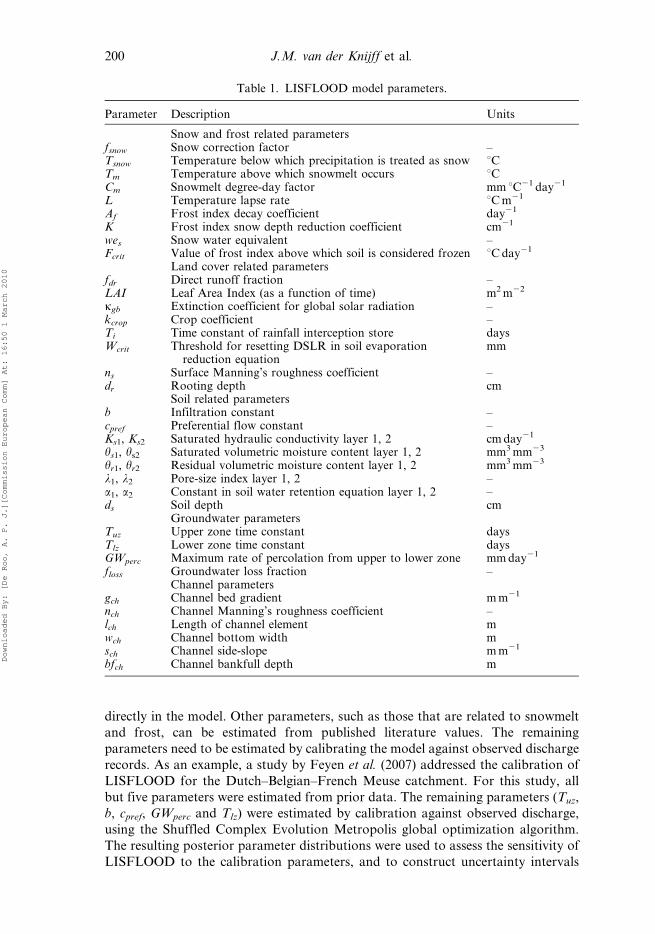
directly in the model. Other parameters, such as those that are related to snowmelt

and frost, can be estimated from published literature values. The remaining

parameters need to be estimated by calibrating the model against observed discharge

records. As an example, a study by Feyen et al. (2007) addressed the calibration of

LISFLOOD for the Dutch–Belgian–French Meuse catchment. For this study, all

but five parameters were estimated from prior data. The remaining parameters (Tuz,

b, cpref, GWperc and Tlz) were estimated by calibration against observed discharge,

using the Shuffled Complex Evolution Metropolis global optimization algorithm.

The resulting posterior parameter distributions were used to assess the sensitivity of

LISFLOOD to the calibration parameters, and to construct uncertainty intervals

Table 1. LISFLOOD model parameters.

Parameter Description Units

Snow and frost related parametersfsnow Snow correction factor –Tsnow Temperature below which precipitation is treated as snow uCTm Temperature above which snowmelt occurs uCCm Snowmelt degree-day factor mm uC21 day21

L Temperature lapse rate uC m21

Af Frost index decay coefficient day21

K Frost index snow depth reduction coefficient cm21

wes Snow water equivalent –Fcrit Value of frost index above which soil is considered frozen uC day21

Land cover related parametersfdr Direct runoff fraction –LAI Leaf Area Index (as a function of time) m2 m22

kgb Extinction coefficient for global solar radiation –kcrop Crop coefficient –Ti Time constant of rainfall interception store daysWcrit Threshold for resetting DSLR in soil evaporation

reduction equationmm

ns Surface Manning’s roughness coefficient –dr Rooting depth cm

Soil related parametersb Infiltration constant –cpref Preferential flow constant –Ks1, Ks2 Saturated hydraulic conductivity layer 1, 2 cm day21

hs1, hs2 Saturated volumetric moisture content layer 1, 2 mm3 mm23

hr1, hr2 Residual volumetric moisture content layer 1, 2 mm3 mm23

l1, l2 Pore-size index layer 1, 2 –a1, a2 Constant in soil water retention equation layer 1, 2 –ds Soil depth cm

Groundwater parametersTuz Upper zone time constant daysTlz Lower zone time constant daysGWperc Maximum rate of percolation from upper to lower zone mm day21

floss Groundwater loss fraction –Channel parameters

gch Channel bed gradient m m21

nch Channel Manning’s roughness coefficient –lch Length of channel element mwch Channel bottom width msch Channel side-slope m m21

bfch Channel bankfull depth m



around the simulated hydrographs. The analysis showed that the model is

particularly sensitive to the parameters that are involved in the generation of fast

runoff: Tuz and cpref, and to a lesser extent also b. Less sensitivity was found for

GWperc and Tlz, which both control slow runoff mechanisms.

In the absence of prior data of sufficient quality it may be necessary to include

other parameters in the calibration procedure. This is no problem, and the model

poses no restrictions on its users as to which parameters are used for calibration and

which ones are ‘fixed’ using prior data. Also, each parameter can be defined either as

a single value, or as a spatially distributed grid. Thus it is possible to account for

within-basin variability, and multiple river basins may even be combined in one

single model run. Another study by Feyen et al. (2008) demonstrates both principles,

using a semi-distributed parameterisation scheme for the calibration of the Czech–

Austrian–Slovak Morava basin. Apart from taking into account the spatial

variation of the calibration parameters, they also included two additional snow-

related parameters in their calibration exercise. The main danger of LISFLOOD’s

flexibility regarding the selection of its calibration parameters is an increased risk of

over-parameterisation problems. However, our experiences with the model so far

have shown that it is very difficult – if not impossible – to define any fixed set of

calibration parameters that ‘work’ in all possible cases. This can be largely explained

by the wide range of climatic and hydrological regimes that can be found across

Europe. For instance, for most catchments in southern Europe LISFLOOD’s snow

and frost related parameters are completely irrelevant, whereas they may control the

dominant hydrological processes in Scandinavia. Nevertheless, over-parameterisation

is a real risk, and it is a good practice to limit the dimensionality of the calibration

exercise by using prior data whenever possible.

4. Technical implementation

LISFLOOD is written in a combination of the PCRaster Dynamic Modelling

Language (Wesseling et al. 1996, Karssenberg 2002) and the Python scripting

language. PCRaster is a raster geographical information system (GIS) that has its

own embedded dynamic programming language. Karssenberg (2002) gives an in-

depth discussion of the advantages of high-level languages such as PCRaster for the

development of distributed hydrological models. It is beyond the scope of this paper

to repeat all his arguments here. In short, in contrast to low-level languages such as

C + + or FORTRAN, PCRaster hides any low-level operations such as file in- and

output and memory management from the programmer, and provides a level of

abstraction that is more at par with the level of thinking of hydrologists. This results

in code that is shorter, easier to read, maintain, modify and re-use. Since all such

operations are handled by generic, highly optimized built-in functions of PCRaster,

this also results in code that is very stable. When a relatively complex model such as

ours is applied to very large datasets this last issue becomes particularly important,

especially if the model is used as part of an operational system (the European Flood

Alert System (EFAS) mentioned in section 5 is a good example of this). Finally,

since PCRaster comes with a host of visualisation tools, these are readily available

to display and analyse LISFLOOD’s output.

In spite of these benefits, until recently some limitations of the software inhibited

the development of a fully operational simulation model in ‘pure’ PCRaster. Most

importantly, an operational setting requires that model users (who may not know

anything about the inner workings of the model) can exert some control over the



model flow. For instance, the EFAS (discussed in section 5) is based entirely on the

analysis of grids of simulated discharge. Most model users will only need discharge

time series at selected gauge locations. Other model users may also be interested in

intermediate state variables, such as soil moisture, and want these as either grids,

time series at points, or spatially averaged values over the area draining to each

gauge location. Reporting all these variables (in all possible formats) would greatly

increase the computation time, as well as the amount of disk space used. Since

PCRaster does not have any mechanisms to let the user activate or disable parts of

the model (such as file write statements) without actually getting into the source

code, this poses some restrictions in an operational setting. We eliminated these

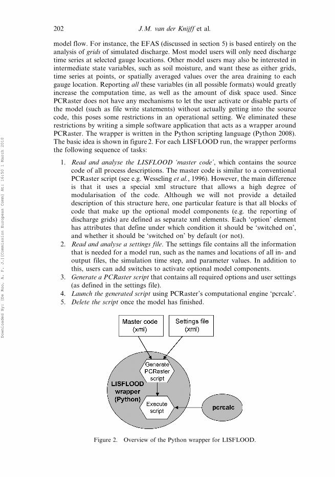
restrictions by writing a simple software application that acts as a wrapper around

PCRaster. The wrapper is written in the Python scripting language (Python 2008).

The basic idea is shown in figure 2. For each LISFLOOD run, the wrapper performs

the following sequence of tasks:

1. Read and analyse the LISFLOOD ‘master code’, which contains the source

code of all process descriptions. The master code is similar to a conventional

PCRaster script (see e.g. Wesseling et al., 1996). However, the main difference

is that it uses a special xml structure that allows a high degree of

modularisation of the code. Although we will not provide a detailed

description of this structure here, one particular feature is that all blocks of

code that make up the optional model components (e.g. the reporting of

discharge grids) are defined as separate xml elements. Each ‘option’ element

has attributes that define under which condition it should be ‘switched on’,

and whether it should be ‘switched on’ by default (or not).

2. Read and analyse a settings file. The settings file contains all the information

that is needed for a model run, such as the names and locations of all in- and

output files, the simulation time step, and parameter values. In addition to

this, users can add switches to activate optional model components.

3. Generate a PCRaster script that contains all required options and user settings

(as defined in the settings file).

4. Launch the generated script using PCRaster’s computational engine ‘pcrcalc’.

5. Delete the script once the model has finished.

Figure 2. Overview of the Python wrapper for LISFLOOD.



One noteworthy feature is that the format of the ‘master code’ is completely generic.

This means that updates or other modifications to the model can be done by

changing the ‘master code’, without any need whatsoever to change the wrapper

routine. Because of this, both maintenance and further development of the code are

just as straightforward as they would be in a ‘native’ PCRaster script.

In order to give a rough indication of LISFLOOD’s computational performance,

we prepared a four-year, daily time-step (1430 steps) water balance simulation for

the full Elbe river basin. At 1-km resolution, this resulted in a simulation grid of

140,309 cells (we will discuss the study area in greater detail in section 6.1). We ran

the simulation under Windows XP Professional on a standard desktop PC with a

2.40 GHz Intel Xeon processor and 1.5 GB internal memory. The total time needed

for this model run was 3 hours and 18 minutes. Computing times of this order of

magnitude may make the use of automatic calibration tools seem somewhat

prohibitive, since such routines typically require hundreds of model runs. However,

because the calibration of LISFLOOD is usually done in a spatially distributed

fashion, large basins such as this one are usually split up in smaller sub-catchments,

each of which is then calibrated separately. The resulting procedure lends itself

perfectly to the use of parallel computing clusters, and in fact these have been used

extensively for most recent calibration work (Feyen et al. 2007, 2008). Currently the

model runs under 32-bit Windows and under a number of Linux distributions. Ports

to other operating systems may follow in the near future.

5. Data management

In this section we will describe what types of data are used with LISFLOOD. We

also explain how the model’s in- and output data can be exchanged with other

software applications.

5.1 Map data

Most input to LISFLOOD is defined in the form of PCRaster maps. Complete sets

of LISFLOOD base maps that cover the whole of Europe have been created at both

1 and 5-km grid resolution. For any given European catchment, a ready-to-use

setup can be created by simply extracting the base maps for the area of interest. This

can be done using PCRaster’s standard data management tools. In addition to this a

set of Python scripts has been written around these tools, which completely

automates the map extraction process. It is also possible to create new LISFLOOD

base maps from scratch, or to edit existing maps. This can be done using any

conventional rater GIS package, such as ArcGIS or GRASS. PCRaster includes

tools for importing and exporting map data from and to a number of ASCII

formats, including ESRI’s popular ASCIIGRID format. In addition, the PCRaster

map format is supported by the Geospatial Data Abstraction Library (GDAL)

library (GDAL 2008). This is an open-source translator library for geospatial raster

data, which can be used for conversions between many different raster formats.

Since all of LISFLOOD’s state and rate variables can be written to maps as well, the

same tools can be used to export the model’s output to other software applications.

A set of custom-made tools has been written for pre-processing and managing the

model’s meteorological input data, which are all fed into the model as stacks of

PCRaster maps. First of all, depending on the data source, raw meteorological data

are either provided as point observations or as interpolated grids. For the former



case, a set of tools and PCRaster scripts is available for the spatial interpolation of

such point data. In the latter case, the aforementioned importer tools can be used.

Second, most meteorological data sets do not provide direct estimates of the

potential evapo(transpi)ration rates ET0, ES0 and EW0. However, these variables

can be derived from the surface radiation budget, which can be calculated from

standard meteorological observations. To this end, a separate pre-processing

application (LISVAP) has been developed, which can be used in conjunction with

LISFLOOD. A detailed description of the LISVAP software can be found in van

der Knijff (2008).

5.2 Table and time series data

Model parameters that are directly linked to soil surface texture and land use classes

are defined in lookup tables, which are plain text files that can be viewed (and

edited, if necessary) in any text editor. All of LISFLOOD’s state and rate variables

can be written to time series as well. Time series are written as plain text files, which

can be easily imported in e.g. spreadsheet software. They can be reported in two

different ways. First, variables can be reported at user-defined locations on a map.

These locations can be either points or areas. In the latter case, the time series file

contains areal averages. Second, at each discharge gauge location, spatial averages

can be calculated. In this case, each variable is averaged over the upstream

contributing area of each gauge. This is particularly useful for getting a summary

view of all components of the water balance at each gauge location.

6. Applications

In this section we will first review some applications of LISFLOOD that have

appeared in the literature. We also present a brief case study for the Elbe catchment.

The model is at the core of the EFAS, which is described in detail by Thielen et al.

(2008) and Ramos et al. (2007). EFAS uses both deterministic and probabilistic

weather forecasts, which are used as input to LISFLOOD. For each forecast,

simulated discharges are evaluated in terms of exceedance of predefined flood alert

thresholds, which are in turn based on a statistical analysis of long-term time series

of simulated discharge. The system was set up to provide early flood warnings in

European transnational river basins, and has been in pre-operational testing mode

since 2005. The whole of Europe is included, and all major European river basins are

combined in one single model setup. Each basin was calibrated using an automatic

algorithm that combines an adaptive partition-based search and a downhill simplex

method (Szabo 2006). A detailed case study of an actual flood event in the Czech

part of the Elbe river basin that was predicted by EFAS can be found in Younis et al.

(2008b). A separate study by Younis et al. (2008a) focuses on the prediction of flash

floods in southern France.

Some recent studies have used the model to evaluate river discharge under a

changing climate. Gouweleeuw et al. (2004) used atmospheric output data from the

rerun of the ECMWF Global Circulation model (ERA40) to force a model run over

the period 1958–2002 for the whole of Europe. This allowed them to generate an

extensive pan-European database of time series of historic river flow. Dankers et al.

(2007) used the climatic output of another, high resolution climate model to

simulate river discharge in the Upper Danube basin in central Europe. Besides a

comparison of simulated discharge for different climatic input resolutions, they also



evaluated various future climate change scenarios. By doing so, they were able to

make some tentative predictions of the impact of future climate changes on the

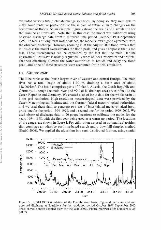
occurrence of floods. As an example, figure 3 shows the results of a simulation for

the Danube at Bratislava. Note that in this case the model was calibrated using

observed discharge data from a different time period (October 1994–September

1997). In terms of long-term water balance, the model shows a good agreement with

the observed discharge. However, zooming in at the August 2002 flood reveals that

in this case the model overestimates the flood peak, and gives a response that is too

fast. These discrepancies can be explained by the fact that the main Danube

upstream of Bratislava is heavily regulated. A series of locks, reservoirs and artificial

channels effectively allowed the water authorities to reduce and delay the flood

peak, and none of these structures were accounted for in this simulation.

6.1 Elbe case study

The Elbe ranks as the fourth largest river of western and central Europe. The main

river has a total length of about 1100 km, draining a basin area of about

148,000 km2. The basin comprises parts of Poland, Austria, the Czech Republic and

Germany, although the main river and 99% of its drainage area are confined to the

Czech Republic and Germany. We created a set of input data for the whole basin at

1-km grid resolution. High-resolution meteorological data were provided by the

Czech Meteorological Institute and the German federal meteorological authorities,

and we used these data to generate two sets of interpolated meteorological input

grids: one for the period 1994–1998, and a second one for the period 1999–2002. We

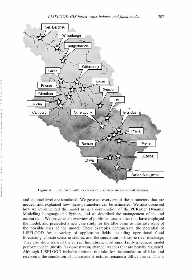
used observed discharge data at 20 gauge locations to calibrate the model for the

years 1994–1998, with the first year being used as a warm-up period. The locations

of the gauges are shown in figure 4. For calibration we used an automatic algorithm

that combines an adaptive partition-based search and a downhill simplex method

(Szabo 2006). We applied the algorithm in a semi-distributed fashion, using spatial

Figure 3. LISFLOOD simulation of the Danube river basin. Figure shows simulated andobserved discharge at Bratislava for the validation period October 1998–September 2002(inset shows a more detailed view for the year 2002). Figure redrawn after Dankers et al.(2007).



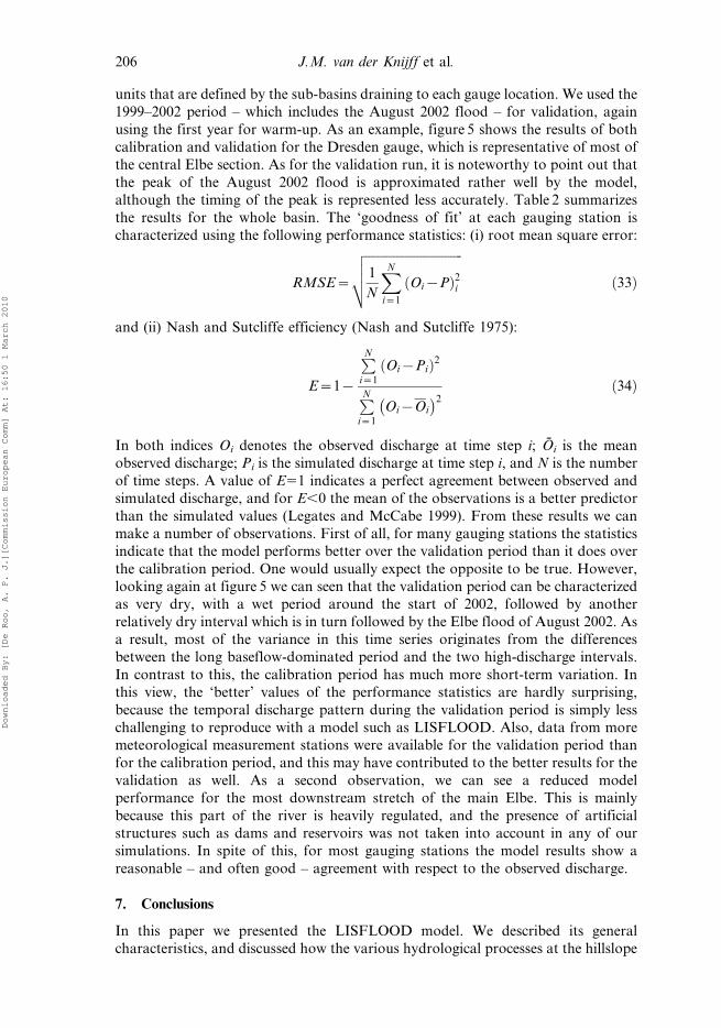
units that are defined by the sub-basins draining to each gauge location. We used the

1999–2002 period – which includes the August 2002 flood – for validation, again

using the first year for warm-up. As an example, figure 5 shows the results of both

calibration and validation for the Dresden gauge, which is representative of most of

the central Elbe section. As for the validation run, it is noteworthy to point out that

the peak of the August 2002 flood is approximated rather well by the model,

although the timing of the peak is represented less accurately. Table 2 summarizes

the results for the whole basin. The ‘goodness of fit’ at each gauging station is

characterized using the following performance statistics: (i) root mean square error:

RMSE~

ffiffiffiffiffiffiffiffiffiffiffiffiffiffiffiffiffiffiffiffiffiffiffiffiffiffiffiffiffiffiffiffi1

N

XN

i~1

Oi{Pð Þ2i

vuut ð33Þ

and (ii) Nash and Sutcliffe efficiency (Nash and Sutcliffe 1975):

E~1{

PN

i~1

Oi{Pið Þ2

PN

i~1

Oi{Oi

� �2ð34Þ

In both indices Oi denotes the observed discharge at time step i; Oi is the mean

observed discharge; Pi is the simulated discharge at time step i, and N is the number

of time steps. A value of E51 indicates a perfect agreement between observed and

simulated discharge, and for E,0 the mean of the observations is a better predictor

than the simulated values (Legates and McCabe 1999). From these results we can

make a number of observations. First of all, for many gauging stations the statistics

indicate that the model performs better over the validation period than it does over

the calibration period. One would usually expect the opposite to be true. However,

looking again at figure 5 we can seen that the validation period can be characterized

as very dry, with a wet period around the start of 2002, followed by another

relatively dry interval which is in turn followed by the Elbe flood of August 2002. As

a result, most of the variance in this time series originates from the differences

between the long baseflow-dominated period and the two high-discharge intervals.

In contrast to this, the calibration period has much more short-term variation. In

this view, the ‘better’ values of the performance statistics are hardly surprising,

because the temporal discharge pattern during the validation period is simply less

challenging to reproduce with a model such as LISFLOOD. Also, data from more

meteorological measurement stations were available for the validation period than

for the calibration period, and this may have contributed to the better results for the

validation as well. As a second observation, we can see a reduced model

performance for the most downstream stretch of the main Elbe. This is mainly

because this part of the river is heavily regulated, and the presence of artificial

structures such as dams and reservoirs was not taken into account in any of our

simulations. In spite of this, for most gauging stations the model results show a

reasonable – and often good – agreement with respect to the observed discharge.

7. Conclusions

In this paper we presented the LISFLOOD model. We described its general

characteristics, and discussed how the various hydrological processes at the hillslope



and channel level are simulated. We gave an overview of the parameters that are

needed, and explained how these parameters can be estimated. We also discussed

how we implemented the model using a combination of the PCRaster DynamicModelling Language and Python, and we described the management of in- and

output data. We provided an overview of published case studies that have employed

the model, and presented a new case study for the Elbe basin to illustrate some of

the possible uses of the model. These examples demonstrate the potential of

LISFLOOD for a variety of application fields, including operational flood

forecasting, climate scenario studies, and the simulation of historic river discharge.

They also show some of the current limitations, most importantly a reduced model

performance in (mostly far downstream) channel reaches that are heavily regulated.Although LISFLOOD includes optional modules for the simulation of lakes and

reservoirs, the simulation of man-made structures remains a difficult issue. This is

Figure 4. Elbe basin with locations of discharge measurement stations.



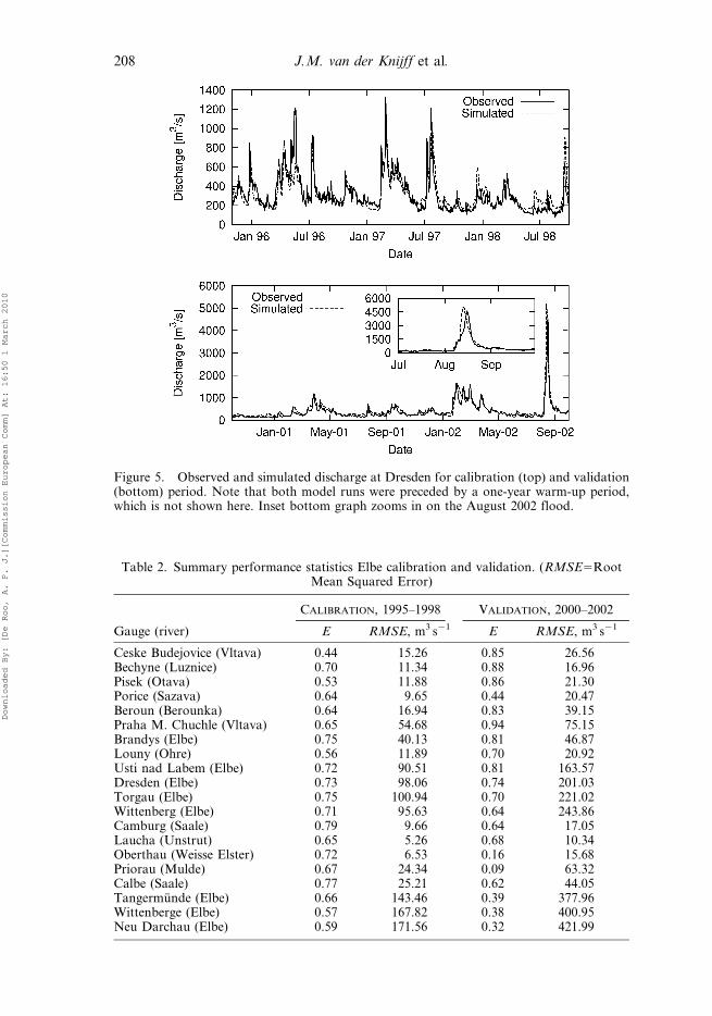
Figure 5. Observed and simulated discharge at Dresden for calibration (top) and validation(bottom) period. Note that both model runs were preceded by a one-year warm-up period,which is not shown here. Inset bottom graph zooms in on the August 2002 flood.

Table 2. Summary performance statistics Elbe calibration and validation. (RMSE5RootMean Squared Error)

Gauge (river)

CALIBRATION, 1995–1998 VALIDATION, 2000–2002

E RMSE, m3 s21 E RMSE, m3 s21

Ceske Budejovice (Vltava) 0.44 15.26 0.85 26.56Bechyne (Luznice) 0.70 11.34 0.88 16.96Pisek (Otava) 0.53 11.88 0.86 21.30Porice (Sazava) 0.64 9.65 0.44 20.47Beroun (Berounka) 0.64 16.94 0.83 39.15Praha M. Chuchle (Vltava) 0.65 54.68 0.94 75.15Brandys (Elbe) 0.75 40.13 0.81 46.87Louny (Ohre) 0.56 11.89 0.70 20.92Usti nad Labem (Elbe) 0.72 90.51 0.81 163.57Dresden (Elbe) 0.73 98.06 0.74 201.03Torgau (Elbe) 0.75 100.94 0.70 221.02Wittenberg (Elbe) 0.71 95.63 0.64 243.86Camburg (Saale) 0.79 9.66 0.64 17.05Laucha (Unstrut) 0.65 5.26 0.68 10.34Oberthau (Weisse Elster) 0.72 6.53 0.16 15.68Priorau (Mulde) 0.67 24.34 0.09 63.32Calbe (Saale) 0.77 25.21 0.62 44.05Tangermunde (Elbe) 0.66 143.46 0.39 377.96Wittenberge (Elbe) 0.57 167.82 0.38 400.95Neu Darchau (Elbe) 0.59 171.56 0.32 421.99



partially because the authorities that are in charge of the operation of such

structures do not always provide all necessary information on the regulation rules.

Also, rules may be complex, they may change over time, or in particular cases they

may not even be followed at all. Because of this, we have not taken this issue into

consideration in the examples presented here. However, with more and better data,

we expect that further improvement may well be possible. This issue should be

addressed in further studies. In section 2 we already mentioned how the simulation

of vertical flow processes in LISFLOOD is always in a downward direction, and

that this may have implications for the use of the model under dry conditions, or in

cases with a profound influence of deep groundwater systems. Current work with

the model has been largely confined to humid, west- and central-European

catchments. Since LISFLOOD was developed with the aim of being applicable

throughout Europe, future studies should investigate the performance of the model

under drier (e.g. Mediterranean) conditions. Also, most current applications have a

strong focus on the simulation of floods; more work is needed to evaluate the

performance of the model during low-flow periods. Both issues will be addressed in

upcoming studies.

Acknowledgements

Over the years of LISFLOOD development, many people have contributed to the

development and testing of the code. We would like to acknowledge in particular the

contributions of Dr. Francesca Somma, Mr. Gian Franchello, Dr. Willem van Deursen

and Mr. Cees Wesseling. Furthermore we would like to thank all our present and past

colleagues at the JRC Floods group for their continuous feedback on the model.

ReferencesALLEN, R.G., PEREIRA, L.S., RAES, D. and SMITH, D., 1998, Crop evapotranspiration –

guidelines for computing crop water requirements. FAO Irrigation and Drainage

Papers, 56.

ASTON, A.R., 1979, Rainfall interception by eight small trees. Journal of Hydrology, 42, pp.

383–396.

BATES, P.D. and DE ROO, A.P.J., 2000, A simple raster-based model for flood inundation

simulation. Journal of Hydrology, 236(1–2), pp. 54–77.

BEVEN, K.J., 2001, Rainfall-runoff Modelling: The Primer (Chichester: John Wiley & Sons).

BEVEN, K.J. and KIRKBY, M.J., 1979, A physically based, variable contributing area model of

basin hydrology. Hydrological Science Bulletin, 24(1), pp. 43–69.

BRUNNER, G.W., 2008, HEC-RAS River Analysis System User’s Manual Version 4.0. Report

CPD-68 (Davis, CA: US Army Corps of Engineers, Hydrologic Engineering Center).

CHOW, V.T., MAIDMENT, D.R. and MAYS, L.M., 1988, Applied Hydrology (Singapore:

McGraw-Hill).

CIARAPICA, L. and TODINI, E., 2002, TOPKAPI: a model for the representation of the

rainfall-runoff process at different scales. Hydrological Processes, 16(2), pp. 207–229.

COMMISSION OF THE EUROPEAN COMMUNITIES (CEC), 1993, CORINE Land Cover, Guide

Technique. EUR 12585EN (Luxemburg: Office for Publications of the European

Communities).

DANKERS, R., BØSSING CHRISTENSEN, O., FEYEN, L., KALAS, M. and DE ROO, A.P.J., 2007,

Evaluation of very high-resolution climate model data for simulating flood hazards in

the Upper Danube Basin. Journal of Hydrology, 347(3–4), pp. 319–331.

DE JONG, S.M. and JETTEN, V.G., 2007, Estimating spatial patterns of rainfall interception

from remotely sensed vegetation indices and spectral mixture analysis. International

Journal of Geographical Information Science, 21(5), pp. 529–545.



DE ROO, A.P.J., WESSELING, C.G. and VAN DEURSEN, W.P.A., 2000, Physically based river

basin modelling within a GIS: The LISFLOOD model. Hydrological Processes, 14,

pp. 1981–1992.

DHI, 2000, MIKE SHE Water Movement –User Manual (Hørsholm: DHI Water and

Environment).

FEYEN, L., VRUGT, J.A., O NUALLAIN, B., VAN DER KNIJFF, J.M. and DE ROO, A.P.J., 2007,

Parameter optimisation and uncertainty assessment for large-scale streamflow

simulation with the LISFLOOD model. Journal of Hydrology, 332, pp. 276–289.

FEYEN, L., KALAS, M. and VRUGT, J., 2008, Semi-distributed parameter optimization and

uncertainty assessment for large-scale streamflow simulation using global optimiza-

tion. Hydrological Sciences Journal, 53(2), pp. 293–308.

GASH, J.H.C., 1979, An analytical model of rainfall interception by forests. Quarterly Journal

of the Royal Meteorological Society, 105, pp. 43–55.

GDAL, 2008, Geospatial Data Abstraction Library. Available online at: http://www.gdal.org/

(accessed 23 June 2008).

GOUWELEEUW, B., THIELEN, J., DE ROO, A.P.J., CLOKE, H., VAN DER KNIJFF, J. and

FRANCHELLO, G., 2004, Evaluation of river flow in Europe over the last 4 decades

using ERA40. In Proceedings SPIE – The International Society for Optical

Engineering, 5568, pp. 92–101.

HAVNØ, K., MADSEN, M.N. and DØRGE, J., 1995, MIKE11 – a generalized river modelling

package. In Computer Models of Watershed Hydrology, V.P. Singh, (Ed.), pp.

733–782, (Colorado: Water Resources Publications).

HIEDERER, R. and DE ROO, A.P.J., 2003, A European Flow Network and Catchment Data Set.

EUR 20703 EN (Luxembourg: Office for Official Publications of the European

Communities).

KARSSENBERG, D., 2002, The value of environmental modelling languages for building

distributed hydrological models. Hydrological Processes, 16, pp. 2751–2766.

KING, D., DAROUSSAIN, J., JAMAGNE, M., LE BAS, C. and MONTANARELLA, L., 1997, The

1:1,000,000 soil geographical database of Europe. In: Bruand, A., Duval, O., Wosten,

J.H.M. and Lilly, A. (eds.), The use of pedotransfer in soil hydrology research in

Europe. INRA Orleans and EC/JRC Ispra.

LEGATES, D.R. and MCCABE, G.J., 1999, Evaluating the use of ‘goodness of fit’ measures in

hydrologic and hydroclimatic model validation. Water resources Research, 35, pp. 233–241.

LINDSTROM, G., JOHANSSON, B., PERSSON, M., GARDELIN, M. and BERGSTROM, S., 1997,

Development and test of the distributed HBV-96 hydrological model. Journal of

Hydrology, 201, pp. 272–288.

MAIDMENT, D.R. (Ed.), 1993, Handbook of Hydrology. McGraw-Hill).

MERRIAM, R.A., 1960, A note on the interception loss equation. Journal of Geophysical

Research, 65, pp. 3850–3851.

MYNENIA, R.B., HOFFMAN, S., KNYAZIKHIN, Y., PRIVETTE, J.L., GLASSY, J., TIAN, Y.,

WANG, Y., SONG, X., ZHANG, Y., SMITH, G.R., LOTSCH, A., FRIEDL, M.,

MORISETTE, J.T., VOTAVA, P., NEMANI, R.R. and RUNNING, S.W., 2002, Global

products of vegetation leaf area and fraction absorbed PAR from year one of MODIS

data. Remote Sensing of Environment, 83(1–2), pp. 214–231.

MOLNAU, M. and BISSELL, V.C., 1983, A continuous frozen ground index for flood

forecasting. In Proceedings 51st Annual Meeting Western Snow Conference, pp.

109–119 (Cambridge, Ont: Canadian Water Resources Assoc.).

NASH, J.E. and SUTCLIFFE, J.V., 1975, River flow forecasting through conceptual models, I: A

discussion of principles. Journal of Hydrology, 10, pp. 282–290.

PYTHON, 2008, Python programming language. Available online at: http://www.python.org

(accessed 23 June 2008).

RAMOS, M.R., BARTHOLMES, J. and THIELEN-DEL-POZO, J., 2007, Development of decision

support products based on ensemble forecasts in the European flood alert system.

Atmospheric Science Letters, 8, pp. 113–119.



RIJKS, D.,TERRES, J.M., and VOSSEN, P. (Eds), 1998, Agrometeorological Applications for

Regional Crop Monitoring and Production Assessment. EUR 17735 EN (Luxembourg:

Office for Official Publications of the European Communities).

RUTTER, A.J., KERSHAW, K.A., ROBINS, P.C. and MORTON, A.J., 1971, Predictive model of

rainfall interception in forests, 1: Derivation of the model from observations in a

plantation of Corsican pine. Agriculture and Meteorology, 9, pp. 367–387.

SCHARFFENBERG, W.A. and FLEMING, M.J., 2008, Hydrologic Modeling System HEC-HMS

User’s Manual Version 3.2. Report CPD-74A (Davis, CA: US Army Corps of

Engineers, Hydrologic Engineering Center).

SPEERS, D.D. and VERSTEEG, J.D., 1979, Runoff forecasting for reservoir operations – the

past and the future. In Proceedings 52nd Western Snow Conference, pp. 149–156 (Fort

Collins, CO: Colorado State University).

STROOSNIJDER, L., 1982, Simulation of the soil water balance. In Simulation of Plant Growth

and Crop Production, Penning de Vries, F.W.T. and van Laar, H.H. (Eds), pp.

175–193, (Wageningen: Simulation Monographs, Pudoc).

STROOSNIJDER, L., 1987, Soil evaporation: Test of a practical approach under semi-arid

conditions. Netherlands Journal of Agricultural Science, 35, pp. 417–426.

SUPIT, I., HOOIJER, A.A., and VAN DIEPEN, C.A. (Eds), 1994, System Description of the

WOFOST 6.0 Crop Simulation Model Implemented in CGMS. Volume 1: Theory and

Algorithms. EUR 15956 (Luxembourg: Office for Official Publications of the

European Communities).

SUPIT, I., and VAN DER Goot, E. (Eds), 2003, Updated System Description of the WOFOST

Crop Growth Simulation Model as Implemented in the Crop Growth Monitoring System

Applied by the European Commission (Heelsum: Treemail).

SZABO, J.A., 2006, An efficient hybrid optimization procedure of adaptive partition-based

search and downhill simplex methods for calibrating water resources models. In

Proceedings of the XXIII Conference of the Danubian Countries on the Hydrological

Forecasting and Hydrological Basis of the Water Management (Belgrade:

Hydrometeorological Institute of Serbia).

THIELEN, J., BARTHOLMES, J., RAMOS, M.-H. and DE ROO, A.P.J., 2008, The European Flood

Alert System – Part 1: Concept and development. Hydrology and Earth System

Sciences Discussions, 5, pp. 257–287.

TODINI, E., 1996, The ARNO rainfall-runoff model. Journal of Hydrology, 175, pp. 339–382.

VAN GENUCHTEN, M.T., 1980, A closed-form equation for predicting the hydraulic conductivity

of unsaturated soils. Soil Science Society of America Journal, 44, pp. 892–898.

VAN DER KNIJFF, J., 2008, LISVAP – Evaporation Pre-Processor for the LISFLOOD Water

Balance and Flood Simulation Model, Revised User Manual, EUR 22639 EN/2

(Luxembourg: Office for Official Publications of the European Communities).

VAN DER KNIJFF, J. and DE ROO, A.P.J., 2008, LISFLOOD – Distributed Water Balance and

Flood Simulation Model, Revised User Manual. EUR 22166 EN/2 (Luxembourg:

Office for Official Publications of the European Communities).

VON HOYNINGEN-HUENE, J., 1981, Die Interzeption des Niederschlags in landwirtschaftlichen

Pflanzenbestanden (Rainfall interception in agricultural plant stands). In

Arbeitsbericht Deutscher Verband fur Wasserwirtschaft und Kulturbau, p.63,

(Braunschweig: DVWK).

WESSELING, C.G., KARSSENBERG, D., BURROUGH, P.A. and VAN DEURSEN, W.P.A., 1996,

Integrating dynamic environmental models in GIS: The development of a dynamic

modelling language. Transactions in GIS, 1, pp. 40–48.

WORLD METEOROLOGICAL ORGANIZATION, 1986, Intercomparison of models of snowmelt

runoff. Operational Hydrology Report 23 (Geneva: World Meteorological Office).

WOSTEN, J.H.M., LILLY, A., NEMES, A. and LE BAS, C., 1999, Development and use of a

database of hydraulic properties of European soils. Geoderma, 90(3–4), pp. 169–185.

YOUNG, G.J. (Ed.) 1985, Techniques for prediction of runoff from glacierized areas

(Wallingford: Institute of Hydrology).



YOUNIS, J., ANQUETIN, S. and THIELEN, J., 2008a, The benefit of high-resolution operational

weather forecasts for flash flood warning. Hydrology and Earth System Sciences, 12,

pp. 1039–1051.

YOUNIS, J., RAMOS, M-H. and THIELEN, J., 2008b, EFAS forecasts for the March-April 2006

flood in the Czech part of the Elbe river basin – a case study. Atmospheric Science

Letters, 9, pp. 88–94.

ZHAO, R.J. and LIU, X.R., 1995, The Xinanjiang model. In Computer Models of Watershed

Hydrology, V.P. Singh, (Ed.), pp. 215–232, (Highlands Ranch, CO: Water Resources

Publications).

212 LISFLOOD GIS-based water balance and flood model


LISFLOOD: a GIS-based distributed model for river basin scale water balance and flood simulation

Documents