Linear response as a singular limit for a periodically driven closed quantum system

This content has been downloaded from IOPscience. Please scroll down to see the full text.

Download details:

IP Address: 117.211.123.51

This content was downloaded on 11/10/2013 at 05:04

Please note that terms and conditions apply.

Linear response as a singular limit for a periodically driven closed quantum system

View the table of contents for this issue, or go to the journal homepage for more

J. Stat. Mech. (2013) P09012

(http://iopscience.iop.org/1742-5468/2013/09/P09012)

Home Search Collections Journals About Contact us My IOPscience

J.Stat.M

ech.(2013)P

09012

ournal of Statistical Mechanics:J Theory and Experiment

Linear response as a singular limit for aperiodically driven closed quantumsystem

Angelo Russomanno1,2, Alessandro Silva1,3 andGiuseppe E Santoro1,2,3

1 SISSA, Via Bonomea 265, I-34136 Trieste, Italy2 CNR-IOM Democritos National Simulation Center, Via Bonomea 265,I-34136 Trieste, Italy3 International Centre for Theoretical Physics (ICTP), PO Box 586,I-34014 Trieste, ItalyE-mail: [email protected], [email protected] and [email protected]

Received 7 June 2013Accepted 20 August 2013Published 13 September 2013

Online at stacks.iop.org/JSTAT/2013/P09012doi:10.1088/1742-5468/2013/09/P09012

Abstract. We address the issue of the validity of linear response theory for aclosed quantum system subject to a periodic external driving. Linear responsetheory (LRT) predicts energy absorption at frequencies of the external drivingwhere the imaginary part of the appropriate response function is different fromzero. Here we show that, for a fairly general nonlinear many-body system ona lattice subject to an extensive perturbation, this approximation should beexpected to be valid only up to a time t∗ depending on the strength of thedriving, beyond which the true coherent Schrodinger evolution departs fromthe linear response prediction and the system stops absorbing energy from thedriving. We exemplify this phenomenon in detail with the example of a quantumIsing chain subject to a time-periodic modulation of the transverse field, bycomparing an exact Floquet analysis with the standard results of LRT. In thiscontext, we also show that if the perturbation is just local, the system is expectedin the thermodynamic limit to keep absorbing energy, and LRT works at alltimes. We finally argue more generally the validity of the scenario presented forclosed quantum many-body lattice systems with a bound on the energy-per-sitespectrum, discussing the experimental relevance of our findings in the context ofcold atoms in optical lattices and ultra-fast spectroscopy experiments.

Keywords: spin chains, ladders and planes (theory), optical lattices, quantumquenches

c© 2013 IOP Publishing Ltd and SISSA Medialab srl 1742-5468/13/P09012+29$33.00

J.Stat.M

ech.(2013)P

09012

Linear response as a singular limit

Contents

1. Introduction 2

2. Linear response theory 4

3. Floquet theory and synchronization 6

4. Energetic considerations: synchronization versus absorption 8

5. Quantum Ising chain under periodic transverse field 10

5.1. Linear response theory approximation for l = L . . . . . . . . . . . . . . . . 11

5.2. Exact evolution and Floquet theory for l = L . . . . . . . . . . . . . . . . . 12

5.3. Comparison of LRT against exact results for l = L . . . . . . . . . . . . . . 13

5.4. Perturbation acting on a subchain of length l < L . . . . . . . . . . . . . . . 18

6. Discussion and conclusions 20

Acknowledgments 22

Appendix A 22

Appendix B 24

Appendix C 25

Appendix D 26

References 28

1. Introduction

Linear response theory (LRT) is one of the most useful tools of statistical physics andcondensed matter theory, both classical and quantum, and is treated in detail in mosttextbooks [1]–[3]. The success of Kubo formulae [4] in describing the response of a systemweakly perturbed out of equilibrium is well known. Its realm of application stretchesfrom transport coefficients in electronic systems [1, 3] to relaxation phenomena in normalliquids, superfluids and magnetic systems [2].

The theory, which is most easily formulated in the quantum case, expresses theresponse of the average value at time t of an observable 〈B〉t for a system whoseHamiltonian H is weakly perturbed by a term v(t)A in terms of (retarded) responsefunctions χBA; the χBA, also known as susceptibilities, are in turn expressed in termsof equilibrium averages of commutators of the Heisenberg operators BH(t) and AH(t′),where the time evolution is assumed to be perfectly unitary (coherent) and governed bythe equilibrium Hamiltonian H.

One of the well known properties of LRT is that it predicts a response which isin general ‘out-of-phase’ with the perturbation—the Fourier transformed susceptibilitiesχ(ω) have imaginary parts—and this is generally associated with energy absorption: the

doi:10.1088/1742-5468/2013/09/P09012 2

J.Stat.M

ech.(2013)P

09012

Linear response as a singular limit

systems take energy from the driving forces at a positive rate controlled by the imaginarypart of the appropriate response functions [1]–[3].

Admittedly, some of the ingredients in the standard derivations of Kubo formulae—such as, for instance, the assumption, in the quantum case, of a perfectly ‘coherent’evolution—are not easy to justify, at least on the macroscopic timescales over whichthe results are successfully applied. Van Kampen has even harshly criticized the wholetheory as a ‘mathematical exercise’ [5] trying to bridge the huge time-gap between theexpected linearity at the macroscopic scale with an unjustified assumption of linearity inthe microscopic equations of motion. Even without taking such an extreme view—afterall, this ‘mathematical exercise’ is remarkably successful—one could still try to test theregime of validity of linear response in the time-domain, in a setting in which a coherentevolution is guaranteed: this might apply both to experiments on cold atoms in opticallattices [6] as well as to more conventional condensed matter systems studied by ultra-fastspectroscopies [7]–[10], where the dynamics of a system in the sub-picosecond range islikely not affected by the interaction with the environment.

An ideal testing ground for LRT is the coherent unitary evolution of a closed many-body quantum system subject to a periodic driving, where a Floquet analysis [11, 12]can be applied provided the usual adiabatic switching-on factors are avoided. In a recentwork [13], we have considered such a problem for a one-dimensional Ising model in atime-dependent uniform transverse field h(t), and found that the response of the systemto a periodic driving of h(t) results—after a transient and in the thermodynamic limit—ina periodic behaviour of the averages of the observables. When considering the transversemagnetization after the transient, in particular, this periodic behaviour turned out to be‘synchronized’ in-phase with the perturbating transverse field, in such a way as to havezero energy absorbed from the driving over a cycle. Though we have exemplified theseideas using a quantum Ising chain, we have argued for their more general validity undercircumstances which could be fairly applicable to closed quantum many-body systems ona lattice in the absence of disorder [13]. A question is, however, in order at this point:‘synchronization’ implies that the out-of-phase response typically associated (within LRT)to energy absorption and the imaginary part of the response functions vanishes. Whatis the physics behind this effect? This is precisely the issue addressed by the presentpaper, where we plan to compare—again, for definiteness, in the quantum Ising chain—the results of an exact Floquet analysis in a regime of weak periodic driving of thetransverse field with the outcome of LRT. We consider both the case of a perturbationwhich is extensive, i.e., involving a number of sites l which increases as the system sizeL in the thermodynamic limit (l, L→∞ but l/L→ constant), as well as that of a localperturbation, where l of order 1. For the case of an extensive perturbation, we find that theresults of LRT are applicable only at short times, and emerge from a rather singular limitin the strength of the perturbation. LRT would predict a constant energy absorbtion at arate proportional to the imaginary part of the corresponding response function. For anysmall but finite perturbation, the true response shows in turn the linear-in-time energyabsorption predicted by LRT only at short times, while eventually at longer times thetrue energy absorption rate vanishes. Correspondingly, of the two components of theLRT—‘in-phase’ and ‘out-of-phase’—only the former survives in the asymptotic limit,corresponding to the ‘synchronization’ of the system with the perturbation. Interestingly,contrary to the dissipative component, the strength of the ‘in-phase’ response turns out

doi:10.1088/1742-5468/2013/09/P09012 3

J.Stat.M

ech.(2013)P

09012

Linear response as a singular limit

to be well described by LRT. This is essentially consistent with what is known in thecontext of mesoscopic physics about the origin of resistance and energy dissipation insmall metallic loops subject to a time-dependent magnetic flux (a uniform electric field):as discussed by Landauer [14] and by Gefen and Thouless [15], due to phase coherence,Zener tunnelling between bands does not imply energy dissipation but rather energystorage [14], and elastic scattering due to localized potentials will generally lead to asaturation of the energy absorbed by the system [15], without resistance (inelastic effectsare essential for that). In our case, we find that in order to describe accurately also thedissipative response with linear response theory the system should act ‘as its own bath’.This happens, for example, when the weak perturbation/driving acts locally in a finiteregion l of order 1: in this case we find that LRT is essentially exact at all times t, asL→∞: the system can accommodate a linear-in-time energy increase (of order 1) evenfor t → ∞, as this adds a vanishingly small contribution to the energy-per-site, of theorder 1/L→ 0.

The rest of the paper is organized as follows. In section 2 we briefly review the LRT,for the reader’s convenience, and present the slightly less common LRT calculation fora perfectly periodic perturbation without adiabatic switching-on factors. In section 3we present the Floquet analysis of a finite amplitude perturbation, and the argumentsleading to an asymptotically periodic behaviour introduced in [13]. Section 4 containssome general energy considerations leading to the conclusions that the true responseoften lacks the ‘out-of-phase’ part predicted by LRT, in particular at least when theperturbation is extensive and the model has a finite bandwidth single-particle spectrum.In section 5 we exemplify these general considerations with a quantum Ising chain subjectto a time-periodic transverse field. We will show, in section 5.3, that, while the LRTresponse proportional to the real part of χ(ω) perfectly matches the exact Floquet resultsfor small driving, the out-of-phase response due to the imaginary part of χ(ω) is, strictlyspeaking, missing at large times. In section 5.4 we discuss the case of a perturbationwhich extends spatially over a segment of the chain of length l, analysing the case inwhich l/L remains constant in the thermodynamic limit (an extensive perturbation), andcontrasting it with the case in which l remains constant (a local perturbation), whereLRT is asymptotically exact. Section 6 contains a summary of our results, a discussionof their experimental relevance, both for cold atoms in optical lattices and for ultra-fastspectroscopies, and our conclusions. Four appendices contain some technical material onthe analysis of the singularities of LRT, on the transverse magnetic susceptibility of thequantum Ising chain, and on the Bogoliubov–de Gennes–Floquet dynamics of a generalinhomogeneous quantum Ising chain.

2. Linear response theory

Let us start with a brief recap of LRT, as discussed in most textbooks [1]–[3]. Assume

that the equilibrium Hamiltonian H0 of a given system is weakly perturbed

H(t) = H0 + v(t)A, (1)

where A is some Hermitian operator and v(t) a (weak) perturbing field. At equilibrium, thesystem would be governed by a thermal (Gibbs) density matrix at a (possibly vanishing)

doi:10.1088/1742-5468/2013/09/P09012 4

J.Stat.M

ech.(2013)P

09012

Linear response as a singular limit

temperature T = 1/(kBβ):

ρeq =∑n

e−βE(0)n

Z

∣∣∣Φ(0)n

⟩⟨Φ(0)n

∣∣∣ , (2)

where∣∣Φ(0)

n

⟩are the eigenstates of H0, E(0)

n the corresponding eigenenergies, and Z =∑ne−βE

(0)n the partition sum. LRT tells us how to calculate the (perturbed) expectation

value of any operator B at time t, 〈B〉t, to linear order in the perturbation v(t), assuming

a coherent (unitary) evolution governed by H(t). Restricting our considerations to the

case B = A, we know that [3]:

〈A〉t = 〈A〉eq +

∫ +∞

−∞dt′ χ(t− t′) v(t′), (3)

where 〈A〉eq = Tr[ρeq A] is the equilibrium value, and the retarded susceptibility χ(t) isgiven by:

χ(t) ≡ − i

~θ(t)

⟨[A(t), A

]⟩eq

= − i

~θ(t)

∑n,m

(ρm − ρn) |Amn|2 e−iωnmt, (4)

with ρn = e−βE(0)n /Z, Amn =

⟨Φ(0)m

∣∣ A ∣∣Φ(0)n

⟩, and ~ωnm = E(0)

n − E(0)m . The relevant

information on the susceptibility is contained in its spectral function

χ′′(ω) = −π~

∑n,m

(ρm − ρn) |Amn|2 δ(ω − ωnm), (5)

which is, essentially, the imaginary part of the Fourier-transform χ(z) for z = ω+ iη, withη → 0+,

χ(z) =

∫ +∞

−∞dt χ(t) eizt =

∫ +∞

−∞

dω

π

χ′′(ω)

ω − z, (6)

and is manifestly odd : χ′′(−ω) = −χ′′(ω). We will always assume (unless otherwise stated)that we are dealing with an extended system in the thermodynamic limit, so that χ′′(ω)is a smooth function of ω, rather than a sum of discrete Dirac delta functions.

Consider now the case of a perfectly periodic perturbation of frequency ω0, fordefiniteness v0 sin(ω0t). The standard textbook approach would include an adiabaticswitching-on of the perturbation from −∞ to 0, writing v(t) = v0 sin(ω0t) [eηtθ(−t) + θ(t)],with a small positive η which is eventually sent to 0 at the end of the calculation. Since weare interested in comparing LRT with a Floquet approach, we insist on a strictly periodicperturbation turned on at t = 0, and take v(t) = vper(t) = v0θ(t) sin(ω0t). The calculationof the response to such a perturbation is an elementary application of equations (3)–(5),and gives:

δ 〈A〉pert = v0

∫ +∞

−∞

dω

2πiχ′′(ω)

(eiω0t − e−iωt

ω + ω0

− e−iω0t − e−iωt

ω − ω0

), (7)

where δ 〈A〉pert = 〈A〉per

t −〈A〉eq. (A word of caution on the notation: δ 〈A〉pert is the response

to the periodic driving vper(t), but is not itself periodic in time.) We notice that, althoughthe usual ±iη factors do not appear anywhere, the integrand in equation (7) is regular,

doi:10.1088/1742-5468/2013/09/P09012 5

J.Stat.M

ech.(2013)P

09012

Linear response as a singular limit

notwithstanding the singular denominators at ω = ±ω0, because the limits for ω → ±ω0

are finite: there is no need, therefore, for a Cauchy principal value prescription. If wesplit the two contributions appearing in the numerators, with e±iω0t and e−iωt, into twoseparate integrals, however, the singularity of the two denominators at ω = ±ω0 willrequire a principal value prescription for both. By using the fact that χ′′(ω) is odd, onereadily finds:

δ 〈A〉pert = v0χ

′(ω0) sin(ω0t)− 2v0ω0−∫ +∞

0

dω

π

χ′′(ω)

ω2 − ω20

sin(ωt), (8)

where we have introduced the Kramers–Kronig transform χ′(ω0)

χ′(ω0) ≡ −∫ +∞

−∞

dω

π

χ′′(ω)

ω − ω0

, (9)

i.e., see equation (6), the real part of χ(ω + iη) on the upper real axis [3].A few comments are in order here. The Riemann–Lebesgue lemma [16] states that

Fourier transforms of a regular function F (ω) (such that |F (ω)| be Lebesgue-integrable)approach 0 for large times

F (t) =

∫dω F (ω)e−iωt t→∞−−−→ 0. (10)

Physically, this result follows from dephasing associated with the overlap of the rapidlyoscillating (for large t) phase-factors e−iωt weighting the ‘smooth’ F (ω). The frequencyintegral appearing in the second term of equation (8), however, has a singularity atω = ω0, which should be treated by the principal value prescription whenever χ′′(ω0) 6= 0.This singularity does not allow a straightforward application of the Riemann–Lebesguelemma, and leads to a large-t value of the integral which does not decay to 0. Indeed,as explained in appendix A, it is a simple matter to ‘extract’ the singularity from theintegral, by isolating a term proportional to χ′′(ω0), which turns out to have the familiarform −v0χ

′′(ω0) cos(ω0t), plus a regular (transient) term F trans(t), ending up with theexpression:

δ 〈A〉pert = v0[χ′(ω0) sin(ω0t)− χ′′(ω0) cos(ω0t)] + F trans(ω0, t), (11)

where the transient part

F trans(ω0, t) = −v0

∫ ∞−∞

dω

π

[χ′′(ω)− χ′′(ω0)]

ω − ω0

sin(ωt), (12)

is now vanishing for large t, due to the Riemann–Lebesgue lemma. Therefore, LRTpredicts a periodic response composed, at large times, of two terms: one in-phase withthe perturbation, proportional to χ′(ω0), and one out-of-phase with it, proportional toχ′′(ω0), associated with energy absorption (see section 4).

3. Floquet theory and synchronization

Let us now discuss the case of a periodic perturbation with a finite, but not necessarilysmall, amplitude. As in [13], the dynamics in this case can be studied using Floquet theory.Let us now, to set the notation, briefly review the basics of Floquet theory, referring

doi:10.1088/1742-5468/2013/09/P09012 6

J.Stat.M

ech.(2013)P

09012

Linear response as a singular limit

the reader to the available literature for more details [11]–[13], [17]. In the case of a

time-periodic Hamiltonian such as equation (1), i.e., H(t) = H(t+ τ) with τ = 2π/ω0, inanalogy with Bloch theorem in the standard band theory of crystalline solids, it is possibleto construct a complete set of solutions of the Schrodinger equation (the Floquet states)which are periodic in time up to a phase

|Ψα (t)〉 = e−iµαt |Φα (t)〉 . (13)

The states |Φα(t)〉, the so-called Floquet modes, are periodic, |Φα(t+ τ)〉 = |Φα(t)〉 whilethe real quantities µα are called Floquet quasi-energies. If we assume that the systemstarts in the density matrix ρ0, we can expand the density matrix at time t in the Floquetbasis. Exploiting the fact that the Floquet states are solutions of the Schrodinger equationwe see that 〈Ψα(t)| ρ(t) |Ψβ(t)〉 = 〈Φα(0)| ρ0 |Φβ(0)〉. Defining ραβ(0) ≡ 〈Φα(0)| ρ0 |Φβ(0)〉we can write

ρ(t) =∑αβ

e−i(µα−µβ)tραβ(0) |Φα(t)〉 〈Φβ(t)| . (14)

The mean value of the operator A at time t is therefore

〈A〉t = Tr[ρ(t)A] =∑αβ

e−i(µα−µβ)tραβ(0)Aβα(t), (15)

where we have defined Aβα(t) = 〈Φβ(t)| A |Φα(t)〉, which is, by construction, a τ -periodicquantity. We can then divide the previous sum into two parts: a periodic part, originatingfrom diagonal elements, and an extra part, originating from off-diagonal elements:

〈A〉t = 〈A〉diagt + 〈A〉off-diag

t . (16)

We can express these two contributions, assuming a non-degenerate Floquet spectrum(µβ 6= µα if β 6= α), as follows4:

〈A〉diagt ≡

∑α

ραα(0)Aαα(t) (17)

〈A〉off-diagt ≡

∫ +∞

−∞

dω

πFt(ω) e−iωt, (18)

where we have introduced the time-dependent τ -periodic weighted joint density of states

Ft(ω) ≡ π∑α6=β

ραβ(0)Aβα(t)δ (ω − µα + µβ) . (19)

Suppose we now evaluate 〈A〉off-diagt at an arbitrary time t0 + nτ , where t0 ∈ [0, τ ]. Since

Ft0+nτ (ω) = Ft0(ω), we can readily find that:

〈A〉off-diagt0+nτ =

∫ +∞

−∞

dω

πFt0(ω) e−iω(t0+nτ),

i.e., exactly of the form to which the Riemann–Lebesgue lemma, equation (10), mightapply. If Ft(ω) is a sufficiently smooth function of ω (such that |Ft(ω)| is Lebesgue-

4 If strict degeneracies are present, the periodic part would get contributions from off-diagonal terms with µβ = µα.See section 5.4 for a discussion of quasi-degeneracies tending to strict degeneracies in the thermodynamic limit inthe case of a local perturbation.

doi:10.1088/1742-5468/2013/09/P09012 7

J.Stat.M

ech.(2013)P

09012

Linear response as a singular limit

integrable) one would conclude that 〈A〉off-diagt decays to 0 after a transient, and the

resulting large-t behaviour of 〈A〉t is asymptotically periodic, 〈A〉t −→ 〈A〉diagt . As

discussed in [13], this occurs whenever the Floquet spectrum is a continuum (in the absenceof singularities). This vanishing of the fluctuating piece, and the resulting time-periodicresponse, will be henceforth referred to as ‘synchronization’ [13]. As we will argue later,this off-diagonal term appears to acquire a singular contribution whenever the driving islocal, thus leading to a steady energy absorption which, however, is not extensive (seesections 4 and 5.4 for a discussion of this point).

4. Energetic considerations: synchronization versus absorption

In the following, we will discuss the physics of energy absorption in a system describedby the generic Hamiltonian H(t) = H0 + v(t)A. For this sake, it is convenient to define

two energy functions: the first, E0(t) = Tr[ρ(t)H0], is the energy of the original system in

the perturbed state ρ(t), while the other, E(t) = Tr[ρ(t)H(t)] = E0(t) + v(t) 〈A〉t, is thetotal energy including the perturbing-field term. Using the fact that a coherent unitaryevolution implies i~ ˙ρ(t) = [H(t), ρ(t)], together with the cyclic property of the trace, it iseasy to derive a Hellmann–Feynman-like formula:

d

dtE(t) = Tr

[ρ(t)

d

dtH(t)

]= v(t) 〈A〉t . (20)

On the other hand, using E0(t) = E(t)−v(t) 〈A〉t, taking a derivative, it is straightforwardto conclude that:

d

dtE0(t) = −v(t)

d

dt〈A〉t . (21)

Consider now for definiteness, v(t) = v0 sin(ω0t) as in section 2. The energy changeduring the nth oscillation of the field, i.e., in the time-window [(n − 1)τ, nτ ], is givenby ∆E(n) = E(nτ)−E((n−1)τ) and ∆E0(n) = E0(nτ)−E0((n−1)τ). Both are directlyobtained from equations (20) and (21) (the second, through integration by parts) andhave the form:

∆E(n) = ∆E0(n) = v0ω0

∫ nτ

(n−1)τ

dt cos(ω0t) 〈A〉t . (22)

If we consider the restriction of 〈A〉t to the nth period time-window [(n− 1)τ, nτ ], call it[〈A〉t]n, we can expand it in a standard Fourier series

[〈A〉t]n = A0(n) ++∞∑m=1

[A(c)m (n) cos(mω0t) + A(s)

m (n) sin(mω0t)], (23)

where the Fourier coefficients A(c,s)m depend in general on the time-window index n, because

the off-diagonal piece 〈A〉off-diagt makes 〈A〉t = 〈A〉diag

t +〈A〉off-diagt to be not strictly periodic.

Evidently, see equation (22), the coefficient A(c)1 (n) of the cos(ω0t) component is what

determines the rate of energy absorption:

Wn =∆E(n)

τ=

1

2v0ω0A

(c)1 (n). (24)

doi:10.1088/1742-5468/2013/09/P09012 8

J.Stat.M

ech.(2013)P

09012

Linear response as a singular limit

LRT predicts in the steady-state (after the decay of the transient equation (11)), an out-

of-phase response with A(c)1 = −v0χ

′′(ω0), which leads to a steady-state (n→∞) increaseof the energy at a rate [3]

WLRTn→∞ = −1

2ω0v

20χ′′(ω0) > 0, (25)

which is positive, since χ′′(ω0 > 0) < 0.As mentioned in section 1, it is well known in the context of mesoscopic physics that

whenever a system is closed, energy absorption resulting from an oscillatory perturbation(for example, in disordered mesoscopic rings) does not correspond to energy dissipation,but rather energy storage [14]. Most importantly, in these systems the energy absorptionrate, which classically would be constant, tends to decrease at long times as a resultof dynamical localization [15]. A steady increase of energy is problematic not only formesoscopic systems but also for closed systems on a lattice, say a fermionic Hubbard-likemodel, the transverse field quantum Ising model, or any spin model in any dimension,whenever A is an extensive operator. Indeed, by simple arguments one can show that thespectrum of such Hamiltonians on a lattice of N = LD sites, D being the dimensionalityof the lattice, should be bounded in a region [eLN, eUN ], where eL and eU are appropriate

finite lower and upper bounds on the energy-per-site. If A is extensive, then a steady(n→∞) and extensive (∝N) energy increase with a rateW , like that predicted by LRT,would inevitably lead to a violation of the boundedness of the spectrum: |E(t)−E(0)|/N <|eU − eL|. Local operators, in contrast, do not lead to an extensive energy increase, anddo not violate any bound. We therefore expect, and explicitly illustrate in the following,that LRT should eventually break down after a while when the perturbation is extensive,even if we are in the thermodynamic limit.

As in the case of mesoscopic systems, also in the case of closed systems on a latticeenergy absorption can be hindered. In particular, this happens if all the observables‘synchronize’ with the perturbing field [13] by showing, after a transient, a perfectly

periodic asymptotic response. When this happens 〈A〉t → 〈A〉diagt and A

(c)1 (n) → 0, for

large n, making the energy absorption rate vanish at large times. In this case the responseis asymptotically ‘in-phase’ with the perturbation:

〈A〉t −→ 〈A〉diagt = A0 + A

(s)1 sin(ω0t) + (higher harmonics), (26)

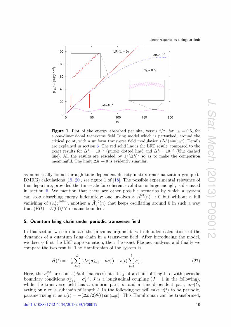
without the out-of-phase term proportional to cos(ω0t). Figure 1 illustrates this with anexplicit calculation performed on the one-dimensional transverse field Ising model, whoseresults will be detailed in section 5. The solid red line represents the energy absorbedper site (E0(t) − E0(0))/L versus the rescaled time t/τ within LRT, for an Ising chainwhose transverse field is uniformly modulated, around the critical point hc = 1, by a term(∆h) sin(ω0t) with ω0 = 0.5, corresponding to a part of the spectrum where χ′′(ω0) 6= 0.Observe the overall linear increase in time with a positive average rate of absorption W ,equation (25), with superimposed small oscillations on the scale of the period τ . The othertwo lines represent the corresponding exact results, obtained from a Floquet analysis,for ∆h = 10−3 and ∆h = 10−2 (all results have been rescaled by 1/(∆h)2 to make thecomparison meaningful). We observe that for any small but finite ∆h the exact resultseventually deviate, for large t, from the linear-in-t LRT prediction, saturating at largetimes up to small and larger-scale oscillations. Similar physics apparently emerges, forinstance, in a periodically modulated homogeneous one-dimensional Hubbard model [18],

doi:10.1088/1742-5468/2013/09/P09012 9

J.Stat.M

ech.(2013)P

09012

Linear response as a singular limit

Figure 1. Plot of the energy absorbed per site, versus t/τ , for ω0 = 0.5, fora one-dimensional transverse field Ising model which is perturbed, around thecritical point, with a uniform transverse field modulation (∆h) sin(ω0t). Detailsare explained in section 5. The red solid line is the LRT result, compared to theexact results for ∆h = 10−2 (purple dotted line) and ∆h = 10−3 (blue dashedline). All the results are rescaled by 1/(∆h)2 so as to make the comparisonmeaningful. The limit ∆h→ 0 is evidently singular.

as numerically found through time-dependent density matrix renormalization group (t-DMRG) calculations [19, 20], see figure 1 of [18]. The possible experimental relevance ofthis departure, provided the timescale for coherent evolution is large enough, is discussedin section 6. We mention that there are other possible scenarios by which a system

can stop absorbing energy indefinitely: one involves a A(c)1 (n) → 0 but without a full

vanishing of 〈A〉off-diagt , another a A

(c)1 (n) that keeps oscillating around 0 in such a way

that (E(t)− E(0))/N remains bounded.

5. Quantum Ising chain under periodic transverse field

In this section we corroborate the previous arguments with detailed calculations of thedynamics of a quantum Ising chain in a transverse field. After introducing the model,we discuss first the LRT approximation, then the exact Floquet analysis, and finally wecompare the two results. The Hamiltonian of the system is

H(t) = −12

L∑j=1

(Jσzjσ

zj+1 + hσxj

)+ v(t)

l∑j=1

σxj . (27)

Here, the σx,zj are spins (Pauli matrices) at site j of a chain of length L with periodicboundary conditions σx,zL+1 = σx,z1 , J is a longitudinal coupling (J = 1 in the following),while the transverse field has a uniform part, h, and a time-dependent part, ∝v(t),acting only on a subchain of length l. In the following we will take v(t) to be periodic,parametrizing it as v(t) = −(∆h/2)θ(t) sin(ω0t). This Hamiltonian can be transformed,

doi:10.1088/1742-5468/2013/09/P09012 10

J.Stat.M

ech.(2013)P

09012

Linear response as a singular limit

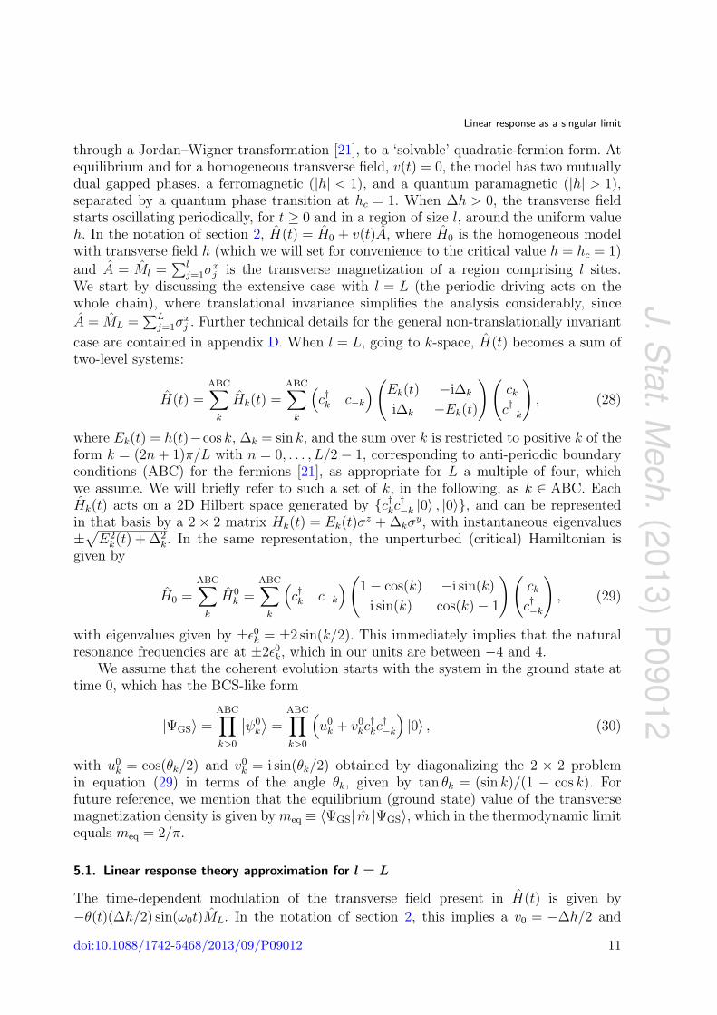
through a Jordan–Wigner transformation [21], to a ‘solvable’ quadratic-fermion form. Atequilibrium and for a homogeneous transverse field, v(t) = 0, the model has two mutuallydual gapped phases, a ferromagnetic (|h| < 1), and a quantum paramagnetic (|h| > 1),separated by a quantum phase transition at hc = 1. When ∆h > 0, the transverse fieldstarts oscillating periodically, for t ≥ 0 and in a region of size l, around the uniform valueh. In the notation of section 2, H(t) = H0 + v(t)A, where H0 is the homogeneous modelwith transverse field h (which we will set for convenience to the critical value h = hc = 1)

and A = Ml =∑l

j=1σxj is the transverse magnetization of a region comprising l sites.

We start by discussing the extensive case with l = L (the periodic driving acts on thewhole chain), where translational invariance simplifies the analysis considerably, since

A = ML =∑L

j=1σxj . Further technical details for the general non-translationally invariant

case are contained in appendix D. When l = L, going to k-space, H(t) becomes a sum oftwo-level systems:

H(t) =ABC∑k

Hk(t) =ABC∑k

(c†k c−k

)(Ek(t) −i∆k

i∆k −Ek(t)

)(ckc†−k

), (28)

where Ek(t) = h(t)−cos k, ∆k = sin k, and the sum over k is restricted to positive k of theform k = (2n + 1)π/L with n = 0, . . . , L/2− 1, corresponding to anti-periodic boundaryconditions (ABC) for the fermions [21], as appropriate for L a multiple of four, whichwe assume. We will briefly refer to such a set of k, in the following, as k ∈ ABC. EachHk(t) acts on a 2D Hilbert space generated by {c†kc

†−k |0〉 , |0〉}, and can be represented

in that basis by a 2 × 2 matrix Hk(t) = Ek(t)σz + ∆kσ

y, with instantaneous eigenvalues±√E2k(t) + ∆2

k. In the same representation, the unperturbed (critical) Hamiltonian isgiven by

H0 =ABC∑k

H0k =

ABC∑k

(c†k c−k

)(1− cos(k) −i sin(k)

i sin(k) cos(k)− 1

)(ckc†−k

), (29)

with eigenvalues given by ±ε0k = ±2 sin(k/2). This immediately implies that the naturalresonance frequencies are at ±2ε0k, which in our units are between −4 and 4.

We assume that the coherent evolution starts with the system in the ground state attime 0, which has the BCS-like form

|ΨGS〉 =ABC∏k>0

∣∣ψ0k

⟩=

ABC∏k>0

(u0k + v0

kc†kc†−k

)|0〉 , (30)

with u0k = cos(θk/2) and v0

k = i sin(θk/2) obtained by diagonalizing the 2 × 2 problemin equation (29) in terms of the angle θk, given by tan θk = (sin k)/(1 − cos k). Forfuture reference, we mention that the equilibrium (ground state) value of the transversemagnetization density is given by meq ≡ 〈ΨGS| m |ΨGS〉, which in the thermodynamic limitequals meq = 2/π.

5.1. Linear response theory approximation for l = L

The time-dependent modulation of the transverse field present in H(t) is given by

−θ(t)(∆h/2) sin(ω0t)ML. In the notation of section 2, this implies a v0 = −∆h/2 and

doi:10.1088/1742-5468/2013/09/P09012 11

J.Stat.M

ech.(2013)P

09012

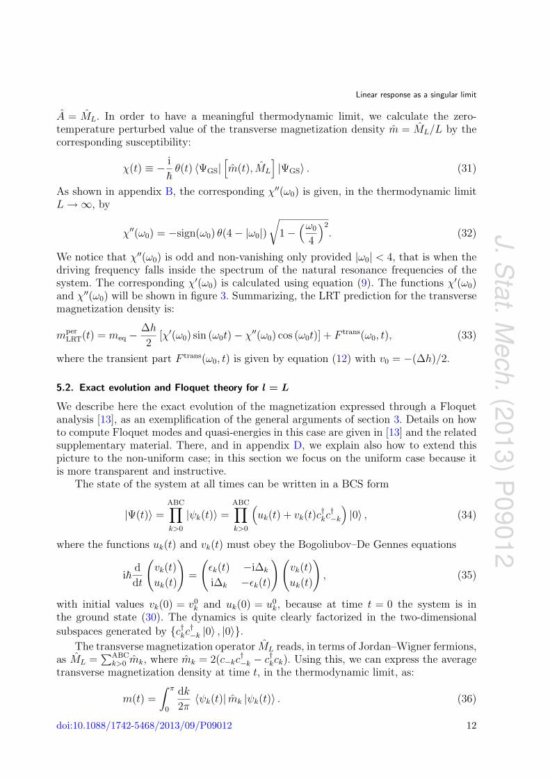
Linear response as a singular limit

A = ML. In order to have a meaningful thermodynamic limit, we calculate the zero-temperature perturbed value of the transverse magnetization density m = ML/L by thecorresponding susceptibility:

χ(t) ≡ − i

~θ(t) 〈ΨGS|

[m(t), ML

]|ΨGS〉 . (31)

As shown in appendix B, the corresponding χ′′(ω0) is given, in the thermodynamic limitL→∞, by

χ′′(ω0) = −sign(ω0) θ(4− |ω0|)√

1−(ω0

4

)2

. (32)

We notice that χ′′(ω0) is odd and non-vanishing only provided |ω0| < 4, that is when thedriving frequency falls inside the spectrum of the natural resonance frequencies of thesystem. The corresponding χ′(ω0) is calculated using equation (9). The functions χ′(ω0)and χ′′(ω0) will be shown in figure 3. Summarizing, the LRT prediction for the transversemagnetization density is:

mperLRT(t) = meq −

∆h

2[χ′(ω0) sin (ω0t)− χ′′(ω0) cos (ω0t)] + F trans(ω0, t), (33)

where the transient part F trans(ω0, t) is given by equation (12) with v0 = −(∆h)/2.

5.2. Exact evolution and Floquet theory for l = L

We describe here the exact evolution of the magnetization expressed through a Floquetanalysis [13], as an exemplification of the general arguments of section 3. Details on howto compute Floquet modes and quasi-energies in this case are given in [13] and the relatedsupplementary material. There, and in appendix D, we explain also how to extend thispicture to the non-uniform case; in this section we focus on the uniform case because itis more transparent and instructive.

The state of the system at all times can be written in a BCS form

|Ψ(t)〉 =ABC∏k>0

|ψk(t)〉 =ABC∏k>0

(uk(t) + vk(t)c

†kc†−k

)|0〉 , (34)

where the functions uk(t) and vk(t) must obey the Bogoliubov–De Gennes equations

i~d

dt

(vk(t)

uk(t)

)=

(εk(t) −i∆k

i∆k −εk(t)

)(vk(t)

uk(t)

), (35)

with initial values vk(0) = v0k and uk(0) = u0

k, because at time t = 0 the system is inthe ground state (30). The dynamics is quite clearly factorized in the two-dimensional

subspaces generated by {c†kc†−k |0〉 , |0〉}.

The transverse magnetization operator ML reads, in terms of Jordan–Wigner fermions,as ML =

∑ABCk>0 mk, where mk = 2(c−kc

†−k − c

†kck). Using this, we can express the average

transverse magnetization density at time t, in the thermodynamic limit, as:

m(t) =

∫ π

0

dk

2π〈ψk(t)| mk |ψk(t)〉 . (36)

doi:10.1088/1742-5468/2013/09/P09012 12

J.Stat.M

ech.(2013)P

09012

Linear response as a singular limit

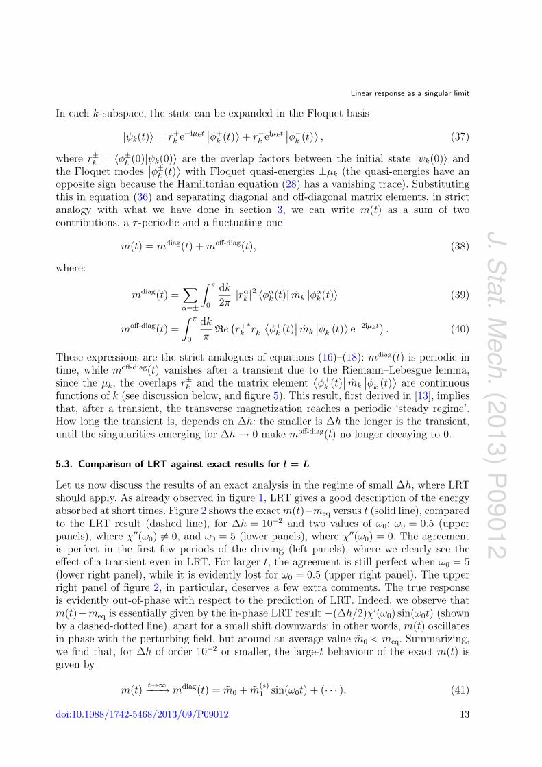
In each k-subspace, the state can be expanded in the Floquet basis

|ψk(t)〉 = r+k e−iµkt

∣∣φ+k (t)

⟩+ r−k eiµkt

∣∣φ−k (t)⟩, (37)

where r±k = 〈φ±k (0)|ψk(0)〉 are the overlap factors between the initial state |ψk(0)〉 andthe Floquet modes

∣∣φ±k (t)⟩

with Floquet quasi-energies ±µk (the quasi-energies have anopposite sign because the Hamiltonian equation (28) has a vanishing trace). Substitutingthis in equation (36) and separating diagonal and off-diagonal matrix elements, in strictanalogy with what we have done in section 3, we can write m(t) as a sum of twocontributions, a τ -periodic and a fluctuating one

m(t) = mdiag(t) +moff-diag(t), (38)

where:

mdiag(t) =∑α=±

∫ π

0

dk

2π|rαk |

2 〈φαk (t)| mk |φαk (t)〉 (39)

moff-diag(t) =

∫ π

0

dk

πRe(r+k∗r−k⟨φ+k (t)

∣∣ mk

∣∣φ−k (t)⟩

e−2iµkt). (40)

These expressions are the strict analogues of equations (16)–(18): mdiag(t) is periodic intime, while moff-diag(t) vanishes after a transient due to the Riemann–Lebesgue lemma,since the µk, the overlaps r±k and the matrix element

⟨φ+k (t)

∣∣ mk

∣∣φ−k (t)⟩

are continuousfunctions of k (see discussion below, and figure 5). This result, first derived in [13], impliesthat, after a transient, the transverse magnetization reaches a periodic ‘steady regime’.How long the transient is, depends on ∆h: the smaller is ∆h the longer is the transient,until the singularities emerging for ∆h→ 0 make moff-diag(t) no longer decaying to 0.

5.3. Comparison of LRT against exact results for l = L

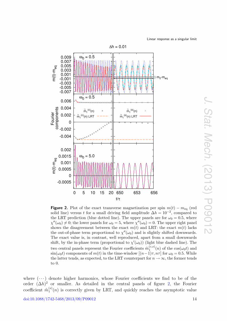
Let us now discuss the results of an exact analysis in the regime of small ∆h, where LRTshould apply. As already observed in figure 1, LRT gives a good description of the energyabsorbed at short times. Figure 2 shows the exact m(t)−meq versus t (solid line), comparedto the LRT result (dashed line), for ∆h = 10−2 and two values of ω0: ω0 = 0.5 (upperpanels), where χ′′(ω0) 6= 0, and ω0 = 5 (lower panels), where χ′′(ω0) = 0. The agreementis perfect in the first few periods of the driving (left panels), where we clearly see theeffect of a transient even in LRT. For larger t, the agreement is still perfect when ω0 = 5(lower right panel), while it is evidently lost for ω0 = 0.5 (upper right panel). The upperright panel of figure 2, in particular, deserves a few extra comments. The true responseis evidently out-of-phase with respect to the prediction of LRT. Indeed, we observe thatm(t)−meq is essentially given by the in-phase LRT result −(∆h/2)χ′(ω0) sin(ω0t) (shownby a dashed-dotted line), apart for a small shift downwards: in other words, m(t) oscillatesin-phase with the perturbing field, but around an average value m0 < meq. Summarizing,we find that, for ∆h of order 10−2 or smaller, the large-t behaviour of the exact m(t) isgiven by

m(t)t→∞−−−→ mdiag(t) = m0 + m

(s)1 sin(ω0t) + (· · · ), (41)

doi:10.1088/1742-5468/2013/09/P09012 13

J.Stat.M

ech.(2013)P

09012

Linear response as a singular limit

Figure 2. Plot of the exact transverse magnetization per spin m(t) −meq (redsolid line) versus t for a small driving field amplitude ∆h = 10−2, compared tothe LRT prediction (blue dotted line). The upper panels are for ω0 = 0.5, whereχ′′(ω0) 6= 0; the lower panels for ω0 = 5, where χ′′(ω0) = 0. The upper right panelshows the disagreement between the exact m(t) and LRT: the exact m(t) lacksthe out-of-phase term proportional to χ′′(ω0) and is slightly shifted downwards.The exact value is, in contrast, well reproduced, apart from a small downwardsshift, by the in-phase term (proportional to χ′(ω0)) (light blue dashed line). Thetwo central panels represent the Fourier coefficients m(c,s)

1 (n) of the cos(ω0t) andsin(ω0t) components of m(t) in the time-window [(n−1)τ, nτ ] for ω0 = 0.5. Whilethe latter tends, as expected, to the LRT counterpart for n→∞, the former tendsto 0.

where (· · · ) denote higher harmonics, whose Fourier coefficients we find to be of theorder (∆h)2 or smaller. As detailed in the central panels of figure 2, the Fourier

coefficient m(s)1 (n) is correctly given by LRT, and quickly reaches the asymptotic value

doi:10.1088/1742-5468/2013/09/P09012 14

J.Stat.M

ech.(2013)P

09012

Linear response as a singular limit

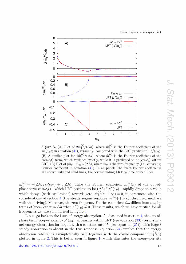
Figure 3. (A) Plot of 2m(s)1 /(∆h), where m(s)

1 is the Fourier coefficient of thesin(ω0t) in equation (41), versus ω0, compared with the LRT prediction −χ′(ω0).(B) A similar plot for 2m(c)

1 /(∆h), where m(c)1 is the Fourier coefficient of the

cos(ω0t) term, which vanishes exactly, while it is predicted to be χ′′(ω0) withinLRT. (C) Plot of (m0−meq)/(∆h), where m0 is the zero-frequency (i.e., constant)Fourier coefficient in equation (41). In all panels, the exact Fourier coefficientsare shown with red solid lines, the corresponding LRT by blue dotted lines.

m(s)1 = −(∆h/2)χ′(ω0) + o(∆h), while the Fourier coefficient m

(c)1 (n) of the out-of-

phase term cos(ω0t)—which LRT predicts to be (∆h/2)χ′′(ω0)—rapidly drops to a value

which decays (with oscillations) towards zero, m(c)1 (n→∞) = 0, in agreement with the

considerations of section 4 (the steady regime response mdiag(t) is synchronized in-phasewith the driving). Moreover, the zero-frequency Fourier coefficient m0 differs from meq byterms of linear order in ∆h when χ′′(ω0) 6= 0. These results, which we have verified for allfrequencies ω0, are summarized in figure 3.

Let us go back to the issue of energy absorption. As discussed in section 4, the out-of-phase term, proportional to χ′′(ω0), appearing within LRT (see equation (33)) results in anet energy absorption for large t with a constant rate W (see equation (25)). This large-tsteady absorption is absent in the true response: equation (24) implies that the energy

absorption rate tends asymptotically to 0 together with the cosine component m(c)1 (n)

plotted in figure 2. This is better seen in figure 1, which illustrates the energy-per-site

doi:10.1088/1742-5468/2013/09/P09012 15

J.Stat.M

ech.(2013)P

09012

Linear response as a singular limit

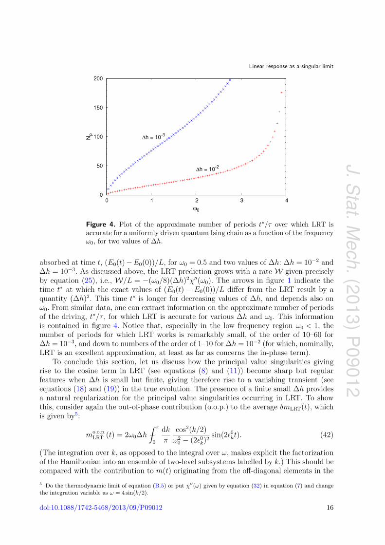
Figure 4. Plot of the approximate number of periods t∗/τ over which LRT isaccurate for a uniformly driven quantum Ising chain as a function of the frequencyω0, for two values of ∆h.

absorbed at time t, (E0(t)−E0(0))/L, for ω0 = 0.5 and two values of ∆h: ∆h = 10−2 and∆h = 10−3. As discussed above, the LRT prediction grows with a rate W given preciselyby equation (25), i.e., W/L = −(ω0/8)(∆h)2χ′′(ω0). The arrows in figure 1 indicate thetime t∗ at which the exact values of (E0(t) − E0(0))/L differ from the LRT result by aquantity (∆h)2. This time t∗ is longer for decreasing values of ∆h, and depends also onω0. From similar data, one can extract information on the approximate number of periodsof the driving, t∗/τ , for which LRT is accurate for various ∆h and ω0. This informationis contained in figure 4. Notice that, especially in the low frequency region ω0 < 1, thenumber of periods for which LRT works is remarkably small, of the order of 10–60 for∆h = 10−3, and down to numbers of the order of 1–10 for ∆h = 10−2 (for which, nominally,LRT is an excellent approximation, at least as far as concerns the in-phase term).

To conclude this section, let us discuss how the principal value singularities givingrise to the cosine term in LRT (see equations (8) and (11)) become sharp but regularfeatures when ∆h is small but finite, giving therefore rise to a vanishing transient (seeequations (18) and (19)) in the true evolution. The presence of a finite small ∆h providesa natural regularization for the principal value singularities occurring in LRT. To showthis, consider again the out-of-phase contribution (o.o.p.) to the average δmLRT(t), whichis given by5:

mo.o.p.LRT (t) = 2ω0∆h −

∫ π

0

dk

π

cos2(k/2)

ω20 − (2ε0k)

2sin(2ε0kt). (42)

(The integration over k, as opposed to the integral over ω, makes explicit the factorizationof the Hamiltonian into an ensemble of two-level subsystems labelled by k.) This should becompared with the contribution to m(t) originating from the off-diagonal elements in the

5 Do the thermodynamic limit of equation (B.5) or put χ′′(ω) given by equation (32) in equation (7) and changethe integration variable as ω = 4 sin(k/2).

doi:10.1088/1742-5468/2013/09/P09012 16

J.Stat.M

ech.(2013)P

09012

Linear response as a singular limit

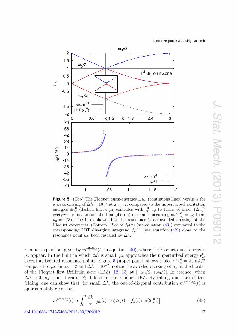
Figure 5. (Top) The Floquet quasi-energies ±µk (continuous lines) versus k fora weak driving of ∆h = 10−2 at ω0 = 2, compared to the unperturbed excitationenergies ±ε0k (dashed lines). µk coincides with ε0k up to terms of order (∆h)2

everywhere but around the (one-photon) resonance occurring at 2ε0k0= ω0 (here

k0 = π/3). The inset shows that the resonance is an avoided crossing of theFloquet exponents. (Bottom) Plot of fk(τ) (see equation (43)) compared to thecorresponding LRT diverging integrand fLRT

k (see equation (42)) close to theresonance point k0, both rescaled by ∆h.

Floquet expansion, given by moff-diag(t) in equation (40), where the Floquet quasi-energiesµk appear. In the limit in which ∆h is small, µk approaches the unperturbed energy ε0k,except at isolated resonance points. Figure 5 (upper panel) shows a plot of ε0k = 2 sin k/2compared to µk for ω0 = 2 and ∆h = 10−2: notice the avoided crossing of µk at the borderof the Floquet first Brillouin zone (1BZ) [12, 13] at [−ω0/2,+ω0/2]. In essence, when∆h → 0, µk tends towards ε0k, folded in the Floquet 1BZ. By taking due care of thisfolding, one can show that, for small ∆h, the out-of-diagonal contribution moff-diag(t) isapproximately given by:

moff-diag(t) ≈∫ π

0

dk

π

[gk(t) cos(2ε0kt) + fk(t) sin(2ε0kt)

], (43)

doi:10.1088/1742-5468/2013/09/P09012 17

J.Stat.M

ech.(2013)P

09012

Linear response as a singular limit

where the two τ -periodic quantities gk(t) and fk(t) originate from the appropriatecombinations of the real and imaginary parts of the matrix element Fk(t) =r+k∗r−k⟨φ+k (t)

∣∣ mk

∣∣φ−k (t)⟩

appearing in equation (40). Both gk(t) and fk(t) are regularfunctions with, at most, a discontinuity across the resonance, while the correspondingLRT integrand fLRT

k = 2ω0∆h cos2(k/2)/[ω20 − (2ε0k)

2] is highly singular and requires aprincipal value prescription. The lower part of figure 5 shows the behaviour of fk(t = τ)compared to its LRT counterpart: quite evidently, there is a finite discontinuity in fk(τ)which develops, for ∆h→ 0, into the singular denominator (ω0−2ε0k)

−1 appearing in LRT.

5.4. Perturbation acting on a subchain of length l < L

Let us now discuss what happens if the perturbation acts only on a segment of thechain of length l < L, coupling to the operator A = Ml previously defined. We denote,from now on, mj = σxj as the transverse magnetization at site j. The LRT predictionis simple, because linearity allows us to study the response on mj′ to a perturbationacting on mj and then appropriately sum the results. The key quantity needed istherefore χ′′j′j(ω), the spectral function associated with the retarded response function

χj′j(t) ≡ −i~−1θ(t) 〈ΨGS| [mj′ (t), mj] |ΨGS〉, from which we can easily reconstruct the

relevant χl(t) = −i~−1θ(t) 〈ΨGS| [Ml(t), Ml] |ΨGS〉. Details are given in appendix C. Notethat χl scales as l in the thermodynamic limit. As for the exact response of the system,we need to apply an inhomogeneous 2L×2L Bogoliubov–de Gennes theory, supplementedby a single-particle Floquet analysis, whose technical details can be found in appendix D.

Once again, we denote by A(c)1 (n) the coefficient of the cos(ω0t) component of 〈Ml〉t

evaluated during the nth period, and by A(s)1 (n) its sin(ω0t) component. As discussed

in section 4, the average energy absorption rate over the nth period is given by Wn =

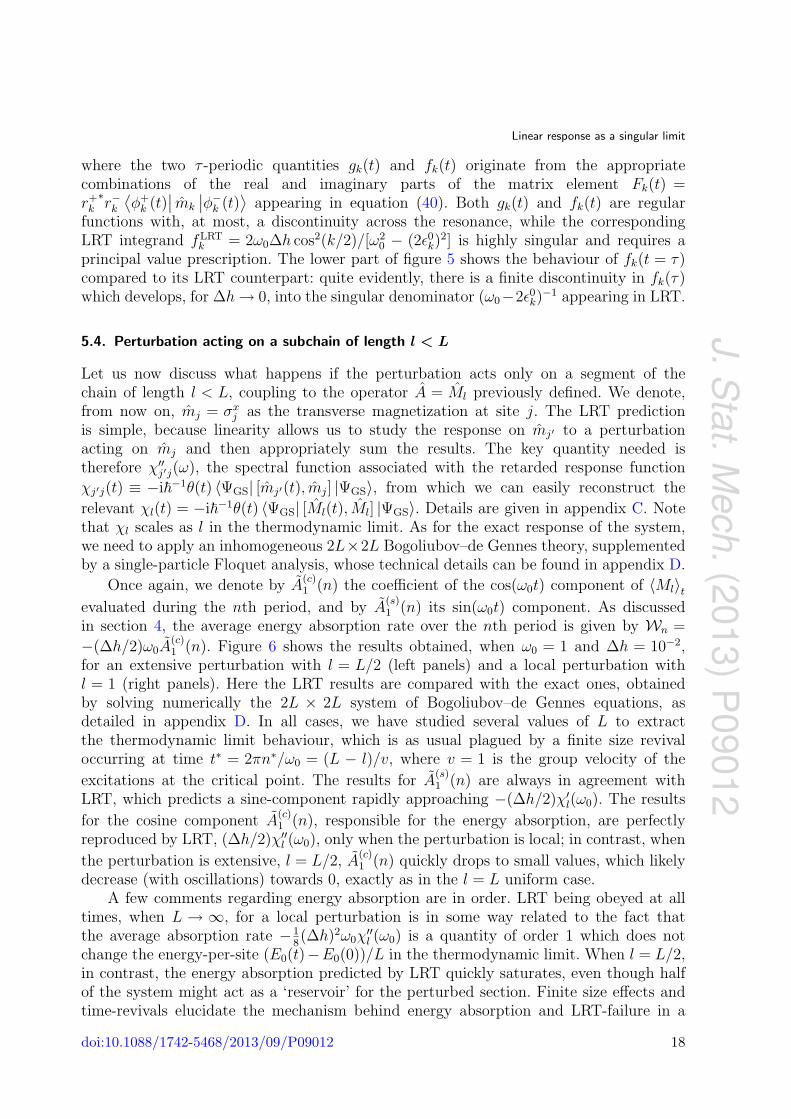
−(∆h/2)ω0A(c)1 (n). Figure 6 shows the results obtained, when ω0 = 1 and ∆h = 10−2,

for an extensive perturbation with l = L/2 (left panels) and a local perturbation withl = 1 (right panels). Here the LRT results are compared with the exact ones, obtainedby solving numerically the 2L × 2L system of Bogoliubov–de Gennes equations, asdetailed in appendix D. In all cases, we have studied several values of L to extractthe thermodynamic limit behaviour, which is as usual plagued by a finite size revivaloccurring at time t∗ = 2πn∗/ω0 = (L − l)/v, where v = 1 is the group velocity of the

excitations at the critical point. The results for A(s)1 (n) are always in agreement with

LRT, which predicts a sine-component rapidly approaching −(∆h/2)χ′l(ω0). The results

for the cosine component A(c)1 (n), responsible for the energy absorption, are perfectly

reproduced by LRT, (∆h/2)χ′′l (ω0), only when the perturbation is local; in contrast, when

the perturbation is extensive, l = L/2, A(c)1 (n) quickly drops to small values, which likely

decrease (with oscillations) towards 0, exactly as in the l = L uniform case.A few comments regarding energy absorption are in order. LRT being obeyed at all

times, when L → ∞, for a local perturbation is in some way related to the fact thatthe average absorption rate −1

8(∆h)2ω0χ

′′l (ω0) is a quantity of order 1 which does not

change the energy-per-site (E0(t)−E0(0))/L in the thermodynamic limit. When l = L/2,in contrast, the energy absorption predicted by LRT quickly saturates, even though halfof the system might act as a ‘reservoir’ for the perturbed section. Finite size effects andtime-revivals elucidate the mechanism behind energy absorption and LRT-failure in a

doi:10.1088/1742-5468/2013/09/P09012 18

J.Stat.M

ech.(2013)P

09012

Linear response as a singular limit

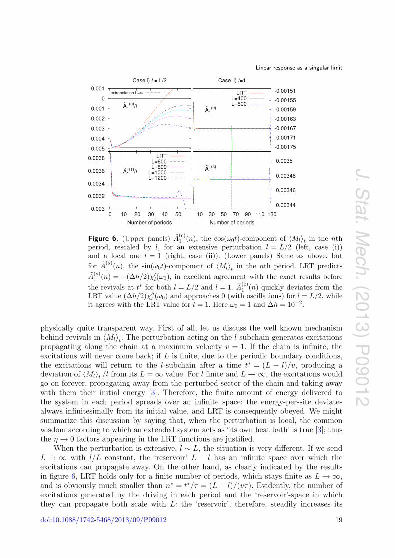
Figure 6. (Upper panels) A(c)1 (n), the cos(ω0t)-component of 〈Ml〉t in the nth

period, rescaled by l, for an extensive perturbation l = L/2 (left, case (i))and a local one l = 1 (right, case (ii)). (Lower panels) Same as above, butfor A(s)

1 (n), the sin(ω0t)-component of 〈Ml〉t in the nth period. LRT predictsA

(s)1 (n) = −(∆h/2)χ′l(ω0), in excellent agreement with the exact results before

the revivals at t∗ for both l = L/2 and l = 1. A(c)1 (n) quickly deviates from the

LRT value (∆h/2)χ′′l (ω0) and approaches 0 (with oscillations) for l = L/2, whileit agrees with the LRT value for l = 1. Here ω0 = 1 and ∆h = 10−2.

physically quite transparent way. First of all, let us discuss the well known mechanismbehind revivals in 〈Ml〉t. The perturbation acting on the l-subchain generates excitationspropagating along the chain at a maximum velocity v = 1. If the chain is infinite, theexcitations will never come back; if L is finite, due to the periodic boundary conditions,the excitations will return to the l-subchain after a time t∗ = (L − l)/v, producing adeviation of 〈Ml〉t /l from its L =∞ value. For l finite and L→∞, the excitations wouldgo on forever, propagating away from the perturbed sector of the chain and taking awaywith them their initial energy [3]. Therefore, the finite amount of energy delivered tothe system in each period spreads over an infinite space: the energy-per-site deviatesalways infinitesimally from its initial value, and LRT is consequently obeyed. We mightsummarize this discussion by saying that, when the perturbation is local, the commonwisdom according to which an extended system acts as ‘its own heat bath’ is true [3]; thusthe η → 0 factors appearing in the LRT functions are justified.

When the perturbation is extensive, l ∼ L, the situation is very different. If we sendL → ∞ with l/L constant, the ‘reservoir’ L − l has an infinite space over which theexcitations can propagate away. On the other hand, as clearly indicated by the resultsin figure 6, LRT holds only for a finite number of periods, which stays finite as L→∞,and is obviously much smaller than n∗ = t∗/τ = (L − l)/(vτ). Evidently, the number ofexcitations generated by the driving in each period and the ‘reservoir’-space in whichthey can propagate both scale with L: the ‘reservoir’, therefore, steadily increases its

doi:10.1088/1742-5468/2013/09/P09012 19

J.Stat.M

ech.(2013)P

09012

Linear response as a singular limit

energy-per-site and the perturbation to the density matrix of the system will cease tobe small: hence the failure of LRT, at least as far as χ′′l is concerned. Surprisingly, sucha failure of LRT is accompanied by an excellent agreement of the χ′l-response. We haveevidence that essentially the same picture holds for all cases with l/L finite.

One final remark concerning the local perturbation case is in order. Assume, fordefiniteness, that we perturb the system on a single site, A = m1, and calculate thecorresponding 〈A〉t. The numerical results shown above, see figure 6, suggest that LRT iscorrect (in the limit of weak driving) at all times; i.e., 〈A〉t develops, after a transient, anout-of-phase component proportional to cos(ω0t), which is periodic but leads to a steadyincrease of the total energy (albeit by a non-extensive quantity). Referring to the generaldiscussion of section 3, we might ask if this periodic but out-of-phase component originatesfrom diagonal or off-diagonal terms in the Floquet expansion. Remarkably, by exploitingthe Heisenberg representation and the Bogoliubov–de Gennes equations, and performing asingle-particle Floquet analysis of the latter (see appendix D), we have a numerical way of

extracting 〈A〉diagt , 〈A〉off-diag

t and its spectral density Ft(ω) (see equations (17)–(19)), whichin principle involve many-body matrix elements and Floquet quasi-energies. Our numericalanalysis suggests that, for every finite size L, there are two-fold quasi-degeneracies ofsingle-particle Floquet quasi-energies µα, (i.e., for every α there is a α 6= α such thatµα ∼ µα) which likely become strict degeneracies for L → ∞, and which appear to bea possible source of a singularity in the spectral function Ft(ω → 0), thus violating thehypothesis of the Riemann–Lebesgue lemma and giving rise to a persisting out-of-phasecontribution.

Summarizing, for a localized perturbation and in the long-time limit, the termsin m1(t) which are diagonal in the Floquet basis contribute only to the in-phaseresponse. Quasi-degenerate off-diagonal terms give a further contribution to the in-phaseresponse, as well as the entire out-of-phase response. These off-diagonal quasi-degeneratecontributions to m1(t) ultimately lead to a periodic response, matching LRT, up to a timet of the same order as the inverse gap among the quasi-degenerate Floquet levels, hencefor longer and longer t as L→∞. This fact mirrors the physical picture that the spacein which we can accommodate excitations grows to infinity in this limit.

6. Discussion and conclusions

The results discussed above have been explicitly demonstrated, so far, just for an Isingchain with a periodically modulated transverse field around the critical point. It is naturalto ask how robust they are in more general circumstances.

The system we explicitly discuss is essentially a free-fermion (BCS) problem. Wouldinteractions between fermions modify this result? Although we have no mathematicalproof for this, we believe that this is not the case. Circumstantial evidence for thisclaim comes from the numerical results of [18], where a Hubbard chain with a hoppingwhich is periodically modulated in time—mimicking fermionic cold atoms experiments—is studied using t-DMRG [19, 20]: the energy absorbed by the system shows clear signsof a saturation similar to that of our figure 1. Admittedly, a fermionic one-dimensionalHubbard model is still integrable (by Bethe-Ansatz ) in equilibrium, but we believe thatintegrability is not a crucial issue in the present context: what we believe crucial (seediscussion in section 4) is that there is a maximum energy-per-site εmax that the system

doi:10.1088/1742-5468/2013/09/P09012 20

J.Stat.M

ech.(2013)P

09012

Linear response as a singular limit

can have, so that 〈Ψ(t)|H0|Ψ(t)〉 < Lεmax at all times, whereas LRT predicts, when χ′′ 6= 0,a steady increase of energy for large t. In view of the energy considerations of section 4,we believe that our results apply, both for extensive and local perturbations, wheneverthe energy-per-site spectrum is bounded; this condition is verified for all the rigid latticesystems.

A word of caution applies to systems (for example a bosonic Hubbard model) thatdo not have a bound on the maximum energy-per-site. An obvious counter-example toour discussion is that of a system of driven harmonic oscillators (masses interacting withnearest-neighbour springs and subject, for instance, to a localized periodic perturbationE(t)x1).6 The linearity of the problem, indeed, makes LRT exact at all times, implyingthat the system will steadily increase its energy in time when the frequency ω0 of thedriving falls inside the natural spectral range of the problem. At the linear level, obviously,Ehrenfest theorem guarantees that quantum and classical physics results coincide. Whennonlinearities are included, for instance adding cubic nearest-neighbour interactions, as inthe Fermi–Pasta–Ulam problem [22], interesting questions emerge concerning classical [23]versus quantum non-equilibrium physics, and deviations from LRT. Although we donot have a full picture of this problem, simulations we have conducted on the classicalFermi–Pasta–Ulam chain with a localized periodic perturbation suggest that, when thenonlinearity is strong enough, there are marked deviations from LRT, but in such a waythat the energy increases in time in a ‘stronger-than-linear’ way, quite differently fromthe saturation effects previously described for quantum systems on a lattice. Regardingclassical versus quantum physics in the phenomena of interest, we stress that boththe bounded energy-per-particle spectrum as well as the role of off-diagonal matrixelements with the accompanying dephasing, are intrinsically quantum ingredients: theeffects described, therefore, might not survive in the classical regime. Equally deservingfurther study are quantum problems on the continuum—where no single-band cut-off,typical of lattice problems, applies—as well as the case of lattice systems in the presenceof phononic modes. In the first case the answer is not obvious: for instance electronsmoving in a continuum crystalline potential have a band energy spectrum without anupper bound; though in some cases [14, 15] quantum coherence effects still forbid energyabsorption beyond a certain limit. We observe also that there is a similarity of our resultswith dynamical localization [24] (quantum coherence and saturation), but in our case athermodynamic limit is essential, while dynamical localization generally applies to systemswhose unperturbed spectrum is characterized by a discrete level spacing.

Finally, let us stress once more the striking difference between a driving which actslocally, where LRT appears to apply at all times, and a driving involving an extensiveperturbation. Evidently, no perturbation can be considered to be ‘small’ at all timesunless the system can act as a ‘its own bath’, which implies that the perturbation shouldnot modify in any essential way the energy-per-site: if there is an infinite space in whichthe finite number of excitations generated by the driving in each period can propagate, theexcitation energy-per-site will be always infinitesimal. In contrast, when the perturbationis extensive, the energy pumped into the system, if no mechanism for dissipation isprovided, will lead to a failure of LRT after a certain finite time: surprisingly enough thereare quantities, like the in-phase response proportional to χ′(ω0) which are well describedby LRT at all times. A non-trivial case might be constituted by systems with localized

6 Here E(t) mimics an electric field acting locally on a single-particle, assumed to possess a dipole moment.

doi:10.1088/1742-5468/2013/09/P09012 21

J.Stat.M

ech.(2013)P

09012

Linear response as a singular limit

states, where the excitations generated by a local perturbation, due to the absence ofdiffusion implied by the localization, cannot propagate away from the perturbed region:the local energy growth might then drive the system away from LRT.

Are the results we have discussed of any relevance to experiments? Obviously,no physical system is perfectly closed: coupling to an environment always leads todecoherence; take for instance the uncontrolled interactions with the electromagnetic fieldof cold atoms in optical lattices, or the coupling of electronic degrees of freedom in asolid to the phononic modes of the lattice. Nevertheless the evolution can be consideredunitary until correlations with the environment set up: this happens after a timescalewhich modern experimental techniques can resolve. For instance, in experiments withcold atoms in optical lattices, coherence times have been attained of ∼ 1 ms [25, 26]; wethink that taking a trapped systems of about 104 atoms (for which we can reasonably talkabout a ‘thermodynamic limit’) a periodic perturbation can be realized and, in principle,with an appropriate choice of ω0, a regime can be reached in which LRT is expectedto hold and where the above-discussed effects can be checked. In the solid state, thedynamics of electrons stays coherent for much shorter timescales, ∼1 ps; nevertheless,even such extremely short timescales are in principle within the experimental reach ofmodern ultra-fast pump-and-probe spectroscopic techniques [7]–[10].

Acknowledgments

We acknowledge discussions with M Fabrizio, C Kollath, J Marino, G Menegoz,P Smacchia, E Tosatti and S Ziraldo. Research was supported by MIUR, through PRIN-2010LLKJBX-001, by SNSF, through SINERGIA Project CRSII2 136287 1, by the EU-Japan Project LEMSUPER, and by the EU FP7 under grant agreement n. 280555. GESdedicates this paper to the dear memory of his friend and mentor Gabriele F Giuliani.

Appendix A

In this appendix we examine the singularities of the LRT susceptibility in the light ofthe standard textbook approach, which includes an adiabatic switching-on factor fort ∈ (−∞, 0]. Consider a periodic perturbing field which is turned on at −∞ as:

v(t) = vswitch(t) + vper(t) = v0 sin(ω0t)[eηtθ(−t) + θ(t)

], (A.1)

where η → 0 at the end of the calculation, and define δ 〈A〉t ≡ 〈A〉t− 〈A〉eq. Since we willconsider only the linear terms in v, we can calculate the two terms separately and add theresults. The switching-on part vswitch(t) = v0θ(−t)eηt sin(ω0t) leads, for t ≥ 0 and η → 0,to:

δ 〈A〉switcht = v0−

∫ +∞

−∞

dω

2πi

(χ′′(ω)

ω + ω0

− χ′′(ω)

ω − ω0

)e−iωt − v0χ

′′(ω0) cos(ω0t), (A.2)

where we made use of the standard approach for dealing with poles in terms of Cauchyprincipal value integrals and Dirac deltas:

limη→0

∫ +∞

−∞dω

f(ω)

ω − ω0 + iη= −∫ +∞

−∞dω

f(ω)

ω − ω0

− iπf(ω0).

doi:10.1088/1742-5468/2013/09/P09012 22

J.Stat.M

ech.(2013)P

09012

Linear response as a singular limit

It is clear that the first integral will have to cancel, for large t, the second term, because,physically, δ 〈A〉switch

t represents the relaxation towards equilibrium after the field wasturned on in (−∞, 0]. Before proceeding with the (simple) mathematical justificationof this statement, let us comment that the Cauchy principal value integral appearingin equation (A.2) is exactly the same, with an opposite sign, as that appearing in theexpression for δ 〈A〉per

t derived in section 2, see equation (8), since

−∫ +∞

−∞

dω

2πi

(χ′′(ω)

ω + ω0

− χ′′(ω)

ω − ω0

)e−iωt = 2ω0−

∫ +∞

0

dω

π

χ′′(ω)

ω2 − ω20

sin(ωt). (A.3)

Therefore, if we sum the two terms we obtain the total response to v(t) as:

δ 〈A〉t = v0 [χ′(ω0) sin(ω0t)− χ′′(ω0) cos(ω0t)] , (A.4)

as indeed expected.We now show that:

v0−∫ +∞

−∞

dω

2πi

(χ′′(ω)

ω + ω0

− χ′′(ω)

ω − ω0

)e−iωt = v0χ

′′(ω0) cos(ω0t) + F relax(ω0, t), (A.5)

where F relax(ω0, t) is a function which relaxes to 0 for t → ∞. First, we see fromequation (5) that χ′′(ω) is non-vanishing only when ω matches a resonance frequencyof the system. We assume we are dealing with a system whose resonance spectrum isa smooth continuum, in which case χ′′(ω) is a regular function. The function χ′′(ω) isodd in ω, so if ω0 falls inside the resonance spectrum χ′′(−ω0) = −χ′′(ω0) 6= 0; if it fallsoutside χ′′(±ω0) = 0. In both cases we can formally split the first term in the integrand(the second term can be treated in the same way)

χ′′(ω)

ω + ω0

e−iωt =χ′′(ω)− χ′′(−ω0)

ω + ω0

e−iωt +χ′′(−ω0)

ω + ω0

e−iωt. (A.6)

The first term is always regular, even for ω → −ω0, and it leads to an integral thatvanishes for large t (Riemann–Lebesgue lemma). Whenever χ′′(±ω0) 6= 0, the second termis singular in −ω0 and contributes to the integral with the part

χ′′(−ω0)−∫ +∞

−∞

dω

2πi

e−iωt

ω + ω0

. (A.7)

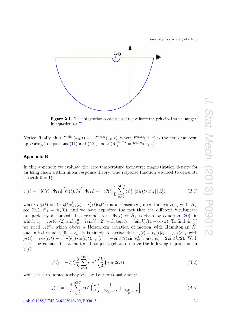
Because of the singularity, this integral does not vanish in the long-time limit, as we aregoing to show by evaluating it with the usual complex plane techniques. Assuming t > 0,we can close the integration contour, both at infinity and around the singularity, in thelower half complex semi-plane, as shown in figure A.1. Using standard techniques, oneconcludes that the principal value integral we need is given by (minus) the contributionaround the singularity (−iπeiω0t/(2πi)), hence:

χ′′(−ω0)−∫ +∞

−∞

dω

2πi

e−iωt

ω + ω0

= −χ′′ (−ω0)

2eiω0t. (A.8)

By repeating this argument for the term with the pole at ω0 and exploiting the fact thatχ′′(ω) is odd in ω, one finally arrives at equation (A.5), where F relax is explicitly given by:

F relax(ω0, t) = v0

∫ ∞−∞

dω

π

[χ′′(ω)− χ′′(ω0)]

ω − ω0

sin(ωt). (A.9)

doi:10.1088/1742-5468/2013/09/P09012 23

J.Stat.M

ech.(2013)P

09012

Linear response as a singular limit

Figure A.1. The integration contour used to evaluate the principal value integralin equation (A.7).

Notice, finally, that F relax(ω0, t) = −F trans(ω0, t), where F trans(ω0, t) is the transient term

appearing in equations (11) and (12), and δ 〈A〉switcht = F relax(ω0, t).

Appendix B

In this appendix we evaluate the zero-temperature transverse magnetization density foran Ising chain within linear response theory. The response function we need to calculateis (with ~ = 1):

χ(t) = −iθ(t) 〈ΨGS|[m(t), M

]|ΨGS〉 = −iθ(t)

1

L

ABC∑k>0

⟨ψk0∣∣ [mk(t), mk]

∣∣ψk0⟩ , (B.1)

where mk(t) = 2(c−k(t)c†−k(t) − c†k(t)ck(t)) is a Heisenberg operator evolving with H0,

see (29), mk = mk(0), and we have exploited the fact that the different k-subspaces

are perfectly decoupled. The ground state |ΨGS〉 of H0 is given by equation (30), inwhich u0

k = cos(θk/2) and v0k = i sin(θk/2) with tan θk = (sin k)/(1− cos k). To find mk(t)

we need ck(t), which obeys a Heisenberg equation of motion with Hamiltonian H0

and initial value ck(0) = ck. It is simple to derive that ck(t) = pk(t)ck + qk(t)c†−k with

pk(t) = cos(ε0kt) − i cos(θk) sin(ε0kt), qk(t) = − sin(θk) sin(ε0kt), and ε0k = 2 sin(k/2). Withthese ingredients it is a matter of simple algebra to derive the following expression forχ(t):

χ(t) = −θ(t) 8

L

ABC∑k>0

cos2

(k

2

)sin(2ε0kt), (B.2)

which in turn immediately gives, by Fourier transforming:

χ(z) = − 4

L

ABC∑k>0

cos2

(k

2

)[1

2ε0k − z+

1

2ε0k + z

]. (B.3)

doi:10.1088/1742-5468/2013/09/P09012 24

J.Stat.M

ech.(2013)P

09012

Linear response as a singular limit

The spectral function χ′′(ω) can be directly extracted from this expression:

χ′′(ω > 0) = −4π

L

ABC∑k>0

cos2

(k

2

)δ(ω − 2ε0k

) L→∞−−−→ −θ(4− ω)

√1−

(ω4

)2

, (B.4)

where we have taken the thermodynamic limit ((1/L)∑ABC

k>0 →∫ π

0 (dk/2π)) whichtransforms the discrete sum of Dirac delta functions into a smooth function.

It is worth mentioning the finite size LRT expression for δ 〈m〉t is immediately obtainedfrom equation (B.2):

δ 〈m〉t = −∆h4

L

ABC∑k>0

cos2

(k

2

)2ε0k sin (ω0t)− ω0 sin (2ε0kt)

ω20 − (2ε0k)

2 . (B.5)

At finite size, there are discrete isolated resonances occurring when ω0 coincides with oneof the excitation frequencies of the unperturbed system: ω0 = 2ε0

k. Such a resonance gives

rise to a quite unphysical prediction of LRT: there is a contribution to δ 〈m〉t originatingfrom the k-term in the sum over k, which can be shown (using de l’Hopital theorem) togrow without bounds in time as −2(∆h)L−1cos2(k/2) t cos(ω0t). Notice that this divergentcontribution carries a 1/L factor. The amusing thing coming out of the thermodynamiclimit is that such isolated resonances are, in some sense, transformed into ‘principal valuesingularities’ which do not give rise to any divergence in δ 〈m〉t, although they are, in theend, responsible for the out-of-phase contribution to δ 〈m〉t, proportional to χ′′(ω0), whichwe have discussed in the text.

Appendix C

In this section we discuss the local susceptibility χj0. The local magnetization operatorsare defined as mj ≡ σxj , and the response function we are interested in can be written as

χj0(t) ≡ − i

~θ(t) 〈ΨGS| [mj(t), m0] |ΨGS〉 . (C.1)

As mentioned in section 2, the crucial information is contained in χ′′j0(ω), which reads:

χ′′j0(ω) = −π~

∑n6=0

[(mj)∗n0(m0)n0 δ (ω − ωn0)− (mj)n0(m0)∗n0 δ (ω − ω0n)] , (C.2)

where the sum extends over the eigenstates (0 labels the ground state); the matrix elements(mj)mn and the frequencies ωmn are defined as in equation (4). As χ′′j0(ω) is odd in ω, weneed to consider only ω ≥ 0. Using the Jordan–Wigner transformation we can write

(mj)n0 = 〈n| mj |ΨGS〉 = − 2

L

∑k,k′

〈n| c†kck′ |ΨGS〉 ei(k′−k)j, (C.3)

where the fermionic operators ck have been defined in section 5. The operators γkdiagonalizing the quadratic Hamiltonian equation (29) can be obtained from the ck with

a Bogoliubov transformation ck = u0kγk + v0

kγ†−k, c

†−k = −v0

k∗γk + u0

kγ†−k. If we substitute

in equation (C.3) we see that the only non-vanishing matrix element is among the ground

doi:10.1088/1742-5468/2013/09/P09012 25

J.Stat.M

ech.(2013)P

09012

Linear response as a singular limit

state and excited states whose form is γ†k′γ†k|ΨGS〉. Applying Wick’s theorem we can write

(mj)n0 = − 2

L

∑k,k′

〈n| c†kck′ |ΨGS〉 ei(k′−k)j = − 2

L

(−u0

k′v0k

+ u0kv0k′

)e−i(k+k′)j, (C.4)

where we have exploited that v0−k = −v0

k and u0−k = u0

k. Substituting this expression inequation (C.2), and using that for the relevant excited states ωn0 = εk + εk′ we can write

χ′′j0(ω ≥ 0) = −π~

4

L2

∑k>k′

∣∣u0kv0k′ − u0

k′v0k

∣∣2 e−i(k+k′)jδ(ω − ε0k− ε0

k′ ), (C.5)

where the condition k > k′ has been enforced to avoid double counting of the excitedstates |n〉. The object inside the sum is symmetric upon exchange of k and k′. Using this,

restricting the sum to the positive k and k′, and going to the thermodynamic limit weget:

χ′′j0(ω ≥ 0) = − 4

π~

∫ π

0

dk

∫ π

0

dk′{|u0kv

0k′ |2 cos(kj) cos(k′j)

− u0k′v0

ku0kv

0k′ sin(kj) sin(k′j)}δ(ω − ε0k − ε0k′ ).

Using the expressions for u0k and v0

k in section 5 and changing variables to ε = 2 sin(k/2),we can rewrite this as:

χ′′j0(ω ≥ 0) = − 1

π~

∫ min(ω,2)

max(0,ω−2)

dε

[√(2− ε)(2 + ε− ω)

(2 + ε)(2 + ω − ε)cos(kεj) cos(kω−εj)

+ sin(kεj) sin(kω−εj)

], (C.6)

where we have defined the function kε ≡ 2 arcsin(ε/2).The linear response function needed in the text is obtained from χj0 via the expression:

χl(t) = − i

~θ(t) 〈ΨGS|

[Ml(t), Ml

]|ΨGS〉 = l

l−1∑j=−l+1

χj0(t). (C.7)

Observe that cancellations in the sum over j, due to the highly oscillating contributionsχj0(t), make χl proportional to l rather than to l2.

Appendix D

In this appendix we briefly describe the quantum dynamics of inhomogeneous Ising/XYchains [27]. Generically, if cj denote the L fermionic operators originating from theJordan–Wigner transformation of spin operators, we can write the Hamiltonian inequation (27) as a quadratic fermionic form

H(t) = Ψ† · H(t) · Ψ =(c† c

)( A(t) B(t)

−B(t) −A(t)

)(c

c†

), (D.1)

doi:10.1088/1742-5468/2013/09/P09012 26

J.Stat.M

ech.(2013)P

09012

Linear response as a singular limit

where Ψ are 2L-components (Nambu) fermionic operators defined as Ψj = cj (for 1 ≤ j ≤L) and ΨL+j = c†j, and H is a 2L× 2L Hermitian matrix having the explicit form shownon the right-hand side, with A an L×L real symmetric matrix and B an L×L real anti-symmetric matrix. Such a form of H implies a particle–hole symmetry: if (uα,vα)T is aninstantaneous eigenvector of H with eigenvalue εα ≥ 0, then (−v∗α,u

∗α)T is an eigenvector

with eigenvalue −εα ≤ 0.Let us now focus on a given time, t = 0, or alternatively suppose that the Hamiltonian

is time-independent. Then, we can apply a unitary Bogoliubov transformation

Ψ =

(c

c†

)= U0 ·

(γ

γ†

)=

(U0 −V∗0V0 U∗0

)·(γ

γ†

), (D.2)

where U0 and V0 are L × L matrices collecting all the eigenvectors of H, by column,turning the Hamiltonian in equation (D.1) in the diagonal form

H =L∑α=1

εα(γ†αγα − γαγ†α

), (D.3)

where the γα are new quasiparticle Fermionic operators. The ground state |GS〉 has energyEGS = −

∑αεα and is the vacuum of the γα for all values of α: 〈GS| γ†αγα |GS〉 = 0.7

To discuss the quantum dynamics when H(t) depends on time, one starts by writing

the Heisenberg’s equations of motion for the Ψ, which turn out to be linear, due to thequadratic nature of H(t). A simple calculation shows that:

i~d

dtΨH(t) = 2H(t) · ΨH(t), (D.4)

the factor 2 on the right-hand side originating from the off-diagonal contributions due to{Ψj,ΨL+j} = 1. These Heisenberg’s equations should be solved with the initial conditionthat, at time t = 0,

ΨH(t = 0) = Ψ = U0 ·(γ

γ†

). (D.5)

A solution is evidently given by

ΨH(t) = U(t) ·(γ

γ†

)(D.6)

with the same γ used to diagonalize the initial t = 0 problem, as long as the time-dependent coefficients U(t) satisfy the ordinary linear Bogoliubov–de Gennes time-dependent equations:

i~d

dtU(t) = 2H(t) · U(t) (D.7)

with initial conditions U(t = 0) = U0. It is easy to verify that the time-dependentBogoliubov–de Gennes form implies that the operators γα(t) in the Schrodinger picture

7 We notice that it would be easy to implement a coherent evolution of a system initially in thermal equilibrium attemperature T = 1/(kBβ), by imposing at time t = 0 that

⟨γ†αγα

⟩0

= 1/(eβεα +1) and going on with the followinganalysis.

doi:10.1088/1742-5468/2013/09/P09012 27

J.Stat.M

ech.(2013)P

09012

Linear response as a singular limit

are time-dependent and annihilate the time-dependent state |ψ(t)〉. Notice that U(t) lookslike the unitary evolution operator of a 2L-dimensional problem with Hamiltonian 2H(t).This implies that one can use a Floquet analysis to get U(t) whenever H(t) is time-periodic. This trick provides us with single-particle Floquet modes and quasi-energies,in terms of which we can reconstruct, through the Heisenberg picture prescription, theexpectation value of an operator 〈ψ(t)|O|ψ(t)〉: it is enough to express O in terms ofthe fermions Ψj, and then use the Heisenberg picture and the (numerical) solution ofthe Bogoliubov–de Gennes equations. For instance, for the transverse magnetizationm = (1/L)

∑Lj=1σ

xj = (1/L)

∑Lj=1(1− 2c†jcj) we immediately get:

m(t) = 〈ψ(t)|m|ψ(t)〉 = 1− 1

L

L∑j,α=1

(|Uj α(t)|2

⟨γ†αγα

⟩0

+ |Vj α(t)|2⟨γαγ

†α

⟩0

), (D.8)

where Ujα(t) = [U(t)]j,α and Vjα(t) = [U(t)]L+j,α. By expanding the Uj α(t) and Vj α(t) inthe corresponding single-particle Floquet modes, we can easily isolate the periodic andthe fluctuating part of m(t).

Further details on the practical implementation of this procedure for the homogeneousIsing case are given in the supplementary material of [13]. In the inhomogeneous case, weaim to find the evolution matrix over one period τ , U(τ), of the 2L× 2L Bogoliubov–deGennes equations (D.7). Notice that, due to the particle–hole form of H(t), it is enoughto solve

i~d

dt

(U(t)

V(t)

)= 2H(t) ·

(U(t)

V(t)

), (D.9)

the full U(t) being given by:

U(t) =

(U(t) −V∗(t)

V(t) U∗(t)

)simplifies our job, allowing us to solve those equations for L different initial conditions(1, . . . , 0︸ ︷︷ ︸

L

| 0, . . . , 0︸ ︷︷ ︸L

)T, . . . , (0, . . . , 1︸ ︷︷ ︸L

| 0, . . . , 0︸ ︷︷ ︸L

)T. Diagonalizing the U(τ) so constructed, we

obtain the quasi-energies as the phases of the eigenvalues. (For numerical reasons, it isbetter to diagonalize the 2L× 2L Hermitian matrix

A = −i (1− U(τ)) (1 + U(τ))−1 . (D.10)

The Floquet quasi-energies are obtained from the 2L eigenvalues aα of A as µα =(ω0/π) atan aα.)

References

[1] Pines D and Nozieres P, 1966 The Theory of Quantum Liquids (New York: Benjamin)[2] Forster D, 1975 Hydrodynamic Fluctuations, Broken Symmetry and Correlation Functions (New York:

Benjamin)[3] Giuliani G F and Vignale G, 2005 Quantum Theory of the Electron Liquid (Cambridge: Cambridge

University Press)[4] Kubo R, Statistical-mechanical theory of irreversible processes. I. General theory and simple applications to

magnetic and conduction problems, 1957 J. Phys. Soc. Japan 12 570

doi:10.1088/1742-5468/2013/09/P09012 28

J.Stat.M

ech.(2013)P

09012

Linear response as a singular limit

[5] van Kampen N G, The case against linear response theory, 1971 Phys. Norv. 5 279[6] Bloch I, Dalibard J and Zwerger W, Many-body physics with ultracold lattices, 2008 Rev. Mod. Phys. 80 885[7] Dantus M and Gross P, 2004 Ultrafast Spectroscopy in Encyclopaedia of Applied Physics (New York:

Wiley)[8] Shah J, 1996 Ultrafast Spectroscopy of Semiconductors and Semiconductor Nanostructures (Berlin:

Springer)[9] Glezer E N, Ultrafast electronic and structural dynamics in solids, 1996 PhD Thesis Harvard University,

Cambridge, MA[10] Nasu K (ed), 2004 Photoinduced Phase Transitions (Singapore: World Scientific)[11] Shirley J H, Solution of Schrodinger equation with a Hamiltonian periodic in time, 1965 Phys. Rev.

138 B979[12] Grifoni M and Hanggi P, Driven quantum tunneling, 1998 Phys. Rep. 304 229[13] Russomanno A, Silva A and Santoro G E, Periodic steady regime and interference in a periodically driven

quantum system, 2012 Phys. Rev. Lett. 109 257201[14] Landauer R, Zener tunneling and dissipation in small loops, 1986 Phys. Rev. B 33 6497[15] Gefen Y and Thouless D J, Zener transitions and energy dissipation in small driven systems, 1987 Phys.

Rev. Lett. 59 1752[16] Bochner S and Chandrasekharan K, 1949 Fourier Transforms (Princeton, NJ: Princeton University Press)[17] Russomanno A, Pugnetti S, Brosco V and Fazio R, Floquet theory of Cooper pair pumping, 2011 Phys. Rev.

B 83 214508[18] Kollath C, Iucci A, McCulloch I and Giamarchi T, Modulation spectroscopy with ultracold fermions in

optical lattices, 2006 Phys. Rev. A 74 041604(R)[19] Daley A J, Kollath C, Schollwock U and Vidal G, Time-dependent density-matrix renormalization-group

using adaptive effective Hilbert spaces, 2004 J. Stat. Mech. P04005[20] White S R and Feiguin A E, Real-time evolution using the density matrix renormalization group, 2004

Phys. Rev. Lett. 93 076401[21] Lieb E, Schultz T and Mattis D, Two soluble models of an antiferromagnetic chain, 1961 Ann. Phys. 16 407[22] Fermi E, Pasta J and Ulam S, Studies of non linear problems, 1955 Los Alamos Report No. LA-1940[23] Castiglione P, Falcioni M, Lesne A and Vulpiani A, 2008 Chaos and Coarse Graining in Statistical

Mechanics (Cambridge: Cambridge University Press)[24] Stockmann H-J, 2007 Quantum Chaos: An Introduction (Cambridge: Cambridge University Press)[25] Sias C, Lignier H, Singh Y P, Zenesini A, Ciampini D, Morsch O and Arimondo E, Observation of photon

assisted tunneling in optical lattices, 2008 Phys. Rev. Lett. 100 040404[26] Lignier H, Sias C, Ciampini D, Singh Y P, Zenesini A, Morsch O and Arimondo E, Dynamical control of

matter-wave tunneling in periodic potentials, 2007 Phys. Rev. Lett. 99 220403[27] Caneva T, Fazio R and Santoro G E, Adiabatic quantum dynamics of a random Ising chain across its

quantum critical point, 2007 Phys. Rev. B 76 144427

doi:10.1088/1742-5468/2013/09/P09012 29