Linear Regression Exploring relationships between two metric variables.

Linear Regression

Exploring relationships between two metric variables

Correlation

• The correlation coefficient measures the strength of a relationship between two variables

• The relationship involves our ability to estimate or predict a variable based on knowledge of another variable

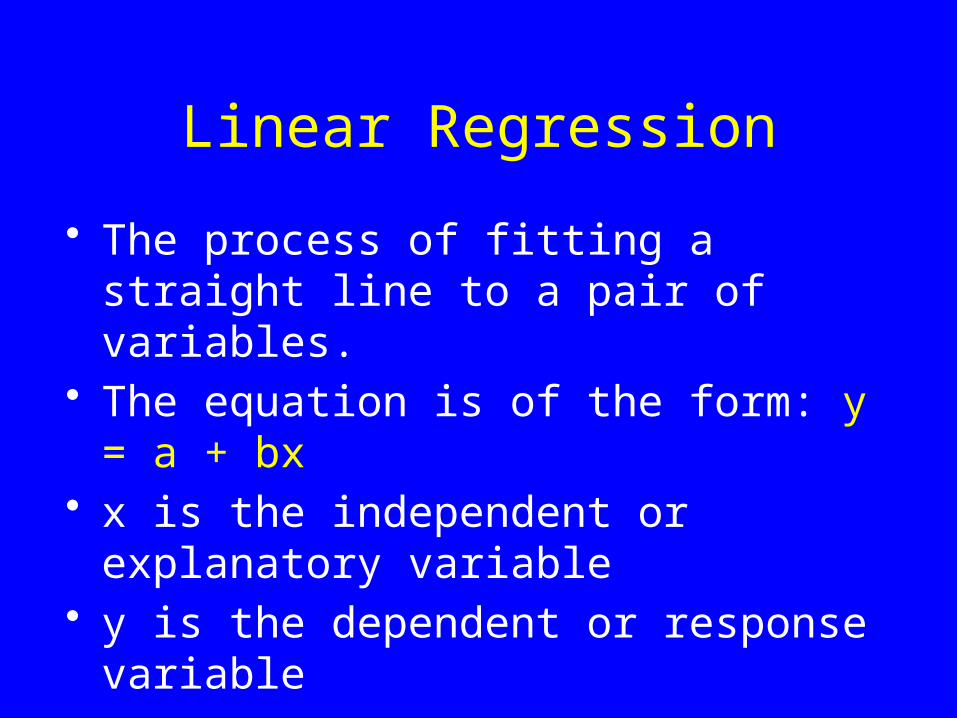
Linear Regression

• The process of fitting a straight line to a pair of variables.

• The equation is of the form: y = a + bx

• x is the independent or explanatory variable

• y is the dependent or response variable

Linear Coefficients

• Given x and y, linear regression estimates values for a and b

• The coefficient a, the intercept, gives the value of y when x=0

• The coefficient b, the slope, gives the amount that y increases (or decreases) for each increase in x

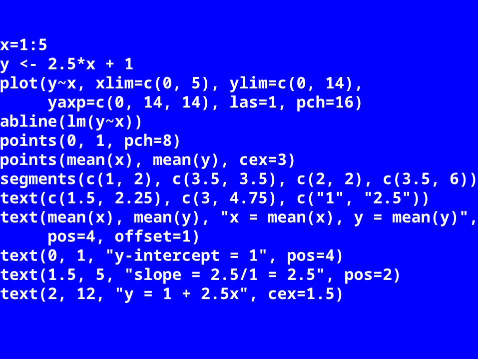
x=1:5y <- 2.5*x + 1plot(y~x, xlim=c(0, 5), ylim=c(0, 14), yaxp=c(0, 14, 14), las=1, pch=16)abline(lm(y~x))points(0, 1, pch=8)points(mean(x), mean(y), cex=3)segments(c(1, 2), c(3.5, 3.5), c(2, 2), c(3.5, 6))text(c(1.5, 2.25), c(3, 4.75), c("1", "2.5"))text(mean(x), mean(y), "x = mean(x), y = mean(y)", pos=4, offset=1)text(0, 1, "y-intercept = 1", pos=4)text(1.5, 5, "slope = 2.5/1 = 2.5", pos=2)text(2, 12, "y = 1 + 2.5x", cex=1.5)

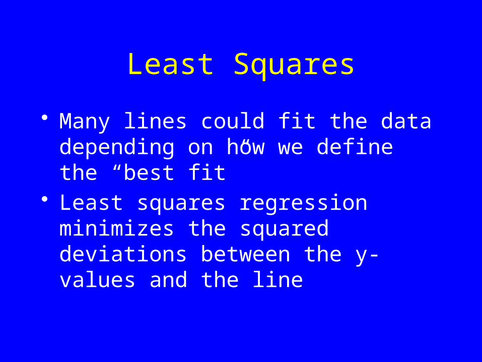
Least Squares

• Many lines could fit the data depending on how we define the “best fit”

• Least squares regression minimizes the squared deviations between the y-values and the line

lm()• Function lm() performs least

squares linear regression in R• Formula used to indicate

Dependent/Response from Independent/Explanatory

• Tilde(~) separates them D~I or R~E

• Rcmdr Statistics | Fit model | Linear regression

> RegModel.1 <- lm(LMS~People, data=Kalahari)> summary(RegModel.1)

Call:lm(formula = LMS ~ People, data = Kalahari)

Residuals: Min 1Q Median 3Q Max -86.400 -24.657 -2.561 24.902 86.100

Coefficients: Estimate Std. Error t value Pr(>|t|) (Intercept) -64.425 44.924 -1.434 0.175161 People 12.868 2.591 4.966 0.000258 ***---Signif. codes: 0 '***' 0.001 '**' 0.01 '*' 0.05 '.' 0.1 ' ' 1

Residual standard error: 47.88 on 13 degrees of freedomMultiple R-squared: 0.6548, Adjusted R-squared: 0.6282 F-statistic: 24.66 on 1 and 13 DF, p-value: 0.0002582

plot(LMS~People, data=Kalahari, pch=16, las=1)RegModel.1 <- lm(LMS~People, data=Kalahari)abline(Line)segments(Kalahari$People, Kalahari$LMS, Kalahari$People, RegModel.1$fitted, lty=2)text(12, 250, paste("y = ", as.character(round(RegModel.1$coefficients[[1]], 2)), " + ", as.character(round(RegModel.1$coefficients[[2]], 2)), "x", sep=""), cex=1.25, pos=4)

Errors

• Linear regression assumes all errors are in the measurement of y

• There are also errors in the estimation of a (intercept) and b (slope)

• Significance for a and b is based on the t distribution

Errors 2

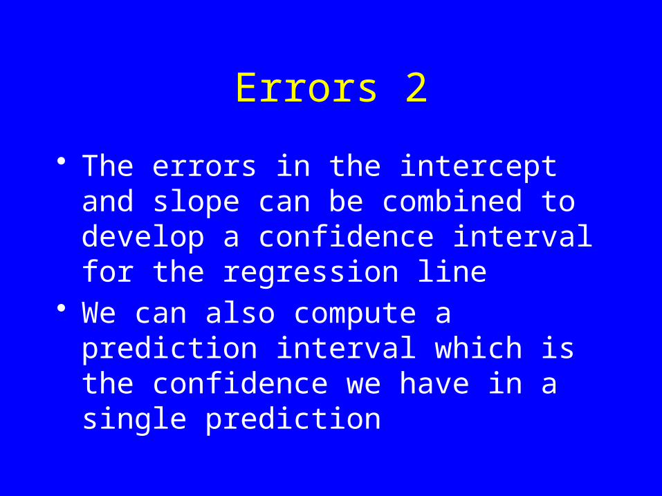
• The errors in the intercept and slope can be combined to develop a confidence interval for the regression line

• We can also compute a prediction interval which is the confidence we have in a single prediction

predict()

• predict() uses the results of a linear regression to predict the values of the dependent/response variable

• It can also produce confidence and prediction intervals:– predict(RegModel.1,

data.frame(People = c(10, 20, 30)), interval="prediction")

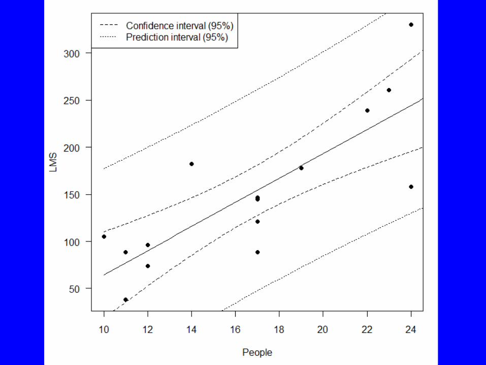
RegModel.1 <- lm(LMS~People, data=Kalahari)plot(LMS~People, data=Kalahari, pch=16, las=1)xp<-seq(10,25,.1)yp<-predict(RegModel.1,data.frame(People=xp),int="c")matlines(xp,yp, lty=c(1,2,2),col="black")yp<-predict(RegModel.1,data.frame(People=xp),int="p")matlines(xp,yp, lty=c(1,3,3),col="black")legend("topleft", c("Confidence interval (95%)", "Prediction interval (95%)"), lty=c(2, 3))

Diagnostics

• Models | Graphs | Basic diagnostic plots– Look for trend in residuals– Look for change in residual variance– Look for deviation from normally

distributed residuals– Look for influential data points

Diagnostics 2

• influence(RegModel.1) returns– Hat (leverage) coefficients– Coefficient changes (leave one out)– Sigma, residual changes (leave one

out)– wt.res, weighted residuals

Other Approaches

• rlm() fits a robust line that is less influenced by outliers

• sma() in package smatr fits standardized major axis (aka reduced major axis) regression and major axis regression – used in allometry