1 Chapter 3: Examining Relationships 3.1Scatterplots 3.2Correlation 3.3Least-Squares Regression.

1

Chapter 3: Examining Relationships

3.1 Scatterplots

3.2 Correlation

3.3 Least-Squares Regression

y = 3.9951x + 4.5711

R2 = 0.9454

181920212223242526

3.5 4.0 4.5 5.0

Fiber Tenacity, g/den

Fabr

ic Te

nacit

y, lb/

oz/yd

^2

2

Relationship Between Fiber Tenacityand Fabric Tenacity

Fiber Tenacity,g/den

Fabric Tenacity,lb/oz/yd2

3.6 19.0

3.9 20.5

4.1 20.8

4.3 21.0

4.8 23.0

5.0 24.9

3

Variable Designations

• Which variable is the dependent variable?

– Our text uses the term response variable.

• Which variable is the independent variable?

– Explanatory variable

• Problems 3.1 and 3.4, p. 123

4

Scatterplot 1: Relationship Between FiberTenacity and Fabric Tenacity

181920212223242526

3.5 4.0 4.5 5.0

Fiber Tenacity, g/den

Fab

ric

Ten

acit

y, lb

/oz/

yd^

2

Note placement of response and explanatory variables. Also noteaxes labels and plot title.

5

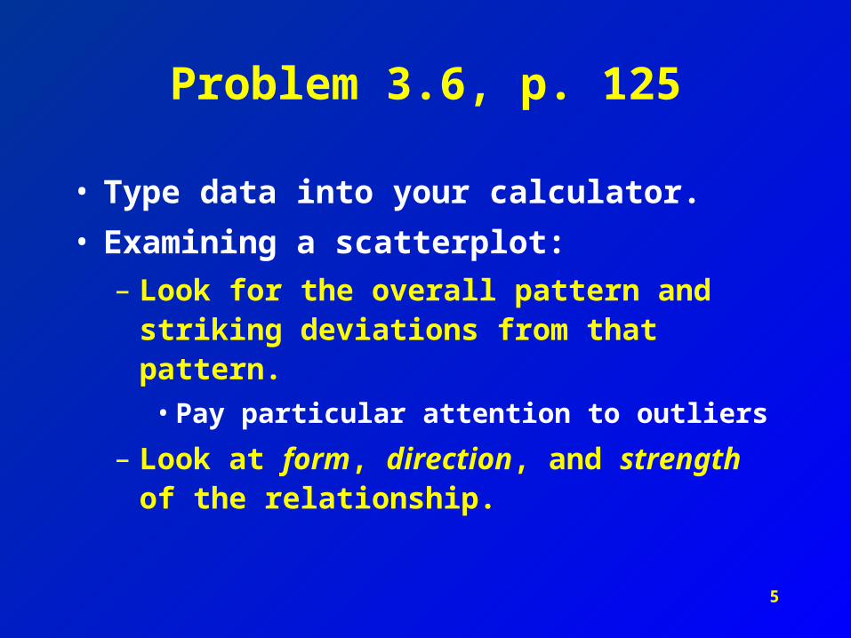
Problem 3.6, p. 125

• Type data into your calculator.

• Examining a scatterplot:

– Look for the overall pattern and striking deviations from that pattern.

• Pay particular attention to outliers

– Look at form, direction, and strength of the relationship.

6

Examining a Scatterplot, cont.

• Form

– Does the relationship appear to be linear?

• Direction

– Positively or negatively associated?

• Strength of Relationship

– How closely do the points follow a clear form?

– In the next section, we will discuss the correlation coefficient as a numerical measure of strength of relationship.

7

Scatterplot for 3.6

8

Problem 3.9, p. 129

9

Tips for Drawing Scatterplots

• p. 128

10

0

10

20

30

40

50

60

60 70 80 90 100 110

Year (67=year 1967)

Inco

me

(Th

ou

san

ds

of

Yea

r 20

00 D

oll

ars)

Black Hispanic White Asian

Adding a Categorical Variable to a Scatterplot

11

Homework

• Reading: pp. 121-135

• Problems:

– 3.11 (p. 129)

– 3.12 (p. 132) … on Excel

– 3.16 (p. 136)

12

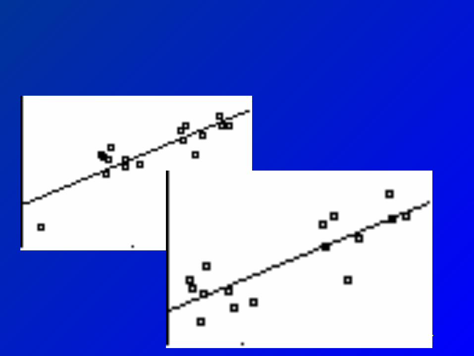
Which shows the strongest

relationship?

800

900

1000

1100

1200

1300

1400

1500

1600

30 40 50 60

200

600

1000

1400

1800

2200

0 20 40 60 80 100 120

13

The two plots represent the same data!

• Our eye is not good enough in describing strength of relationship.

– We need a method for quantifying the relationship between two variables.

• The most common measure of relationship is the Pearson Product Moment correlation coefficient.

– We generally just say “correlation coefficient.”

14

Correlation Coefficient, r

• The correlation, r, is an average of the products of the standardized x-values and the standardized y-values for each pair.

y

in

i x

i

s

yy

s

xx

nr

11

1

15

Correlation Coefficient, r

• A correlation coefficient measures these characteristics of

the linear relationship between two variables, x and y.

– Direction of the relationship

• Positive or negative

– Degree of the relationship: How well do the data fit the

linear form being considered?

• Correlation of (1 or -1) represents a perfect fit.

• Correlation of (0) indicates no relationship.

16

Interpreting Correlation Coefficient, r

• Correlation Applet: http://www.duxbury.com/authors/mcclellandg/tiein/johnson/correlation.htm

• Facts about correlation

– pp.143-144

• Correlation is not a complete description of two-variable data. We also need to report a complete numerical summary (means and standard deviations, 5-number summary) of both x and y.

17

Exercise

• 3.25, p. 146

18

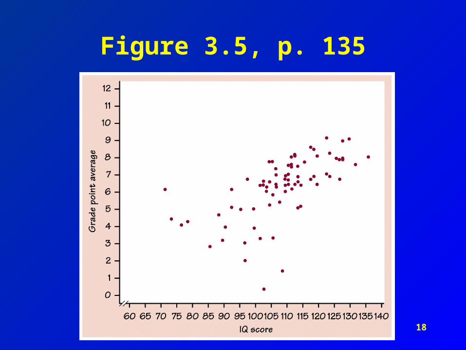
Figure 3.5, p. 135

19

Figure 3.6, p. 136

20

Outlier, or influential point?

• Let’s enter the data into our calculators and calculate the correlation coefficient. The data are in the middle two columns of Table 1.10, p. 59.

– r=?

• Now, remove the possible influential point. What happens to r?

21

22

Exercises: Understanding Correlation

• Review “Facts about correlation,” pp. 143-144

• 3.34, 3.35, and 3.37, p. 149

• Reading: pp. 149-157

23

Relationship Between Winding Tensionand Yarn Elongation

y = -0.0759x + 9.4455

R2 = 0.732

6.0

6.5

7.0

7.5

8.0

8.5

9.0

10 15 20 25 30 35

Winding Tension, g

Elongation%

24(e)error yyresidual^

i

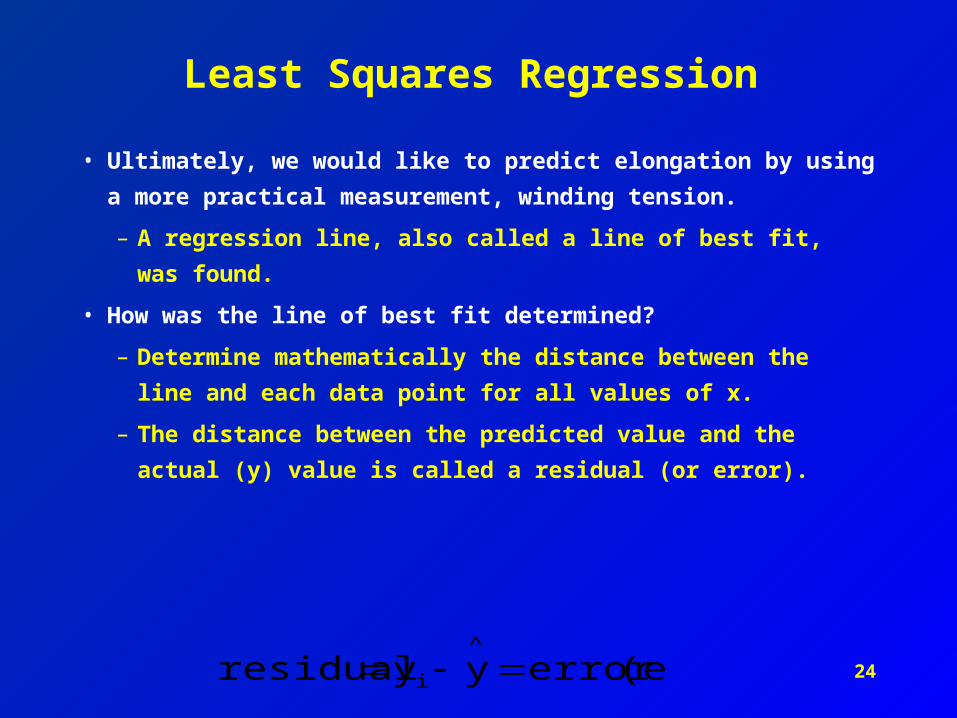
Least Squares Regression

• Ultimately, we would like to predict elongation by using a

more practical measurement, winding tension.

– A regression line, also called a line of best fit, was found.

• How was the line of best fit determined?

– Determine mathematically the distance between the line

and each data point for all values of x.

– The distance between the predicted value and the actual

(y) value is called a residual (or error).

25

n

1i

2^

i2 )y(ye

• The best-fitting line is the line that has the smallest sum of e2 ... the least squares regression line! That is, the line of best fit occurs when:

minimum )y(yen

1i

2^

i2

Least Squares Regression: Line of Best Fit

• This could be done for each data point. If we square each residual and sum all of the squared residuals, we have:

26

A Residual (Figure 3.11, p. 151)

27

bxa ^

y

Least-Squares Regression Line

• With the help of algebra and a little calculus, it can be

shown that this occurs when:

x

y

s

srb

xbya

28

Exercise 3.12, p. 132

• Is there a relationship between lean body mass and resting metabolic rate for females?

– Quantify this relationship.

• Find the line of best fit (the least-squares regression, LSR).

• Use the LSR to predict the resting metabolic rate for a woman with mass of 45 kg and for a woman with mass of 59.5 kg.

29

Interpreting the Regression Model

• The slope of the regression line is important for the interpretation of the data:

– The slope is the rate of change of the response variable with a one unit change in the explanatory variable.

• The intercept is the value of y-predicted when x=0. It is statistically meaningful only when x can actually take values close to zero.

30r = 0.85, r2 = 0.72

1- r2 = 0.28

R2: Coefficient of Determination

• Proportion of variability in one variable that can be

associated with (or predicted by) the variability of the

other variable.

31

Exercise 3.45, p. 166

32

Exercise 3.45, p. 166

33

Back to residuals …

• In regression, we see deviations by looking at the scatter of points about the regression line. The vertical distances from the points to the least-squares regression line are as small as possible, in the sense that they have the smallest possible sum of squares.

• Because they represent “left-over” variation in the response after fitting the regression line, these distances are called residuals.

34

Examining the Residuals

• The residuals show how far the data fall from our regression line, so examining the residuals helps us to assess how well the line describes the data.

– Residuals Plot

35

Residuals Plot

• Let’s construct a residuals plot, that is, a plot of the explanatory variable vs. the residuals.

– pp. 174-175

• The residuals plot helps us to assess the fit of the least squares regression line.

– We are looking for similar spread about the line y=0 (why?) for all levels of the explanatory variable.

36

Residuals Plot Interpretation, cont.

• A curved or other definitive pattern shows an underlying relationship that is not linear.

– Figure 3.19(b), p. 170

• Increasing or decreasing spread about the line as x increases indicates that prediction of y will be less accurate for smaller or larger x.

– Figure 3.19(c), p. 171

• Look for outliers!

37

Figures 3.19 (a-c), pp. 170-171

38

How to create a residuals plot• Create regression model using your calculator.

• Create a column in your STAT menu for residuals. Remember that a residual is the actual value minus the predicted value:

yyresidual

39

Residuals Plot for 3.45

40

HW

• Read through end of chapter

• Problems:

– 3.42 and 3.43, p. 165

– 3.46, p. 173

• Chapter 3 Test on Friday

41

Regression Outliers and Influential Observations

• A regression outlier is an observation that lies outside the overall pattern of the other observations.

• An observation is influential for a statistical calculation if removing it would markedly change the result of the calculation.– Points that are outliers in the x direction of a scatterplot are

often influential for the least-squares regression line.• Sometimes, however, the point is not influential when it falls in

line with the remaining data points.

– Note: An influential point may be an outlier in terms of x, but we label it as “influential” if removing it significantly influences the regression.

42

Practice Problems

• Problems:

– 3.56, p. 179

– 3.74, p. 188

– 3.76, p. 189

43

Preparing for the Test

• Re-read chapter.

– Know the terms, big concepts.

• Chapter Review, pp. 181-182

• Go back over example and HW problems.

• Study slides!