Lincoln Laboratory - Defense Technical Information Center · Lincoln Laboratory MASSACHUSETTS INSTITUTE OF TECHNOLOGY H ... skyward was computed using Eq. (1) and the published radio

D RECORD COPY SCIENTIFIC DIVISION

ES7 !>#.

Copy No. £_ jL cys

Technical Note 1966-59

Noise Temperature of Airborne Antennas at UHF

G. Ploussios

6 December 1966

Lincoln Laboratory MASSACHUSETTS INSTITUTE OF TECHNOLOGY H

Lexington, Massachns ;i s

• .

The work reported in this document was performed at Lincoln Laboratory, a center for research operated by Massachusetts Institute of Technology, with the support of the U.S. Air Force under Contract AF 19(628)-5167.

This report may be reproduced to satisfy needs of U.S. Government agencies.

Distribution of this document is unlimited.

165

MASSACHUSETTS INSTITUTE OF TECHNOLOGY

LINCOLN LABORATORY

NOISE TEMPERATURE OF AIRBORNE ANTENNAS AT UHF

G. PLOUSSIOS

Group 62

TECHNICAL NOTE 1966-59

6 DECEMBER 1966

LEXINGTON MASSACHUSETTS

ABSTRACT

Partial results of an experimental program to determine the electro-

magnetic noise environment at UHF on board an aircraft are presented.

Contributors to an airborne receiver noise temperature including galactic

noise, earth temperature, P-static, atmospherics and industrial noise were

measured and are discussed. A model of the industrial noise is presented

whereby the industrial area is considered as a uniformly distributed source

of independent radiators, the magnitude being the same for all cities

measured with the exception of the New York City area.

RFI generated by on-board equipment and/or ground transmitters will

be covered in a subsequent report.

Accepted for the Air Force Franklin C. Hudson Chief, Lincoln Laboratory Office

111

NOISE TEMPERATURE OF AIRBORNE ANTENNAS AT UHF

I. INTRODUCTION

The noise level of an airborne UHF receiver is ultimately limited by

the receive antenna temperature. In order to characterize this limit a three -

part experimental program was initiated. The first two portions of the pro-

gram provided the necessary data to describe continuous and transient noise

levels inherent to an airborne system. The third portion of the program

(still in progress), deals with man-made coherent radiation. This source

of noise will be covered in a subsequent report.

Electromagnetic radiation originating from the earth, atmosphere

and galaxy all contribute to the antenna temperature, the relative importance

of each source being dependent upon antenna illumination. Equivalent expres-

sions for determining antenna temperature, using the radio astronomers'

terminology, are shown below.

Ta=W?TB. DH> M i 1

where:

T = antenna terminal temperature due to noise sources external to the antenna

TR = brightness temperature in solid angle £2. i

D(£2.) = normalized receive antenna radiation pattern over solid angle £2.

I

G = antenna gain o °

277 17/2

77/2 Ta = "4¥ J I _,, TB(<

where T^id^) = Brightness temperature as a function of the spherical

co-ordinates 9 and 0

D(9,0) = normalized receive antenna radiation pattern

9 = elevation angle measured from the horizon.

In the following sections measured values of the brightness tempera-

ture of the various sources illuminated by the receive antenna are presented.

The frequency, time and geographical dependence of these sources are dis-

cussed. In addition, equations and curves are derived relating the effect of

noise generated in industrial areas, city noise, on the receive antenna

temperature.

Data was taken at three frequencies, 226. 2 MHz, 305. 5 MHz and

369. 2 MHz using total power radiometers, each with a 1. 2 MHz bandwidth

and 2 msec integration. A C-135 jet aircraft and a C-131 propeller type

aircraft were the test vehicles. A UHF blade (monopole) antenna, the AT/256,

mounted on the top of the fuselage was used on the C-135. This antenna pro-

duced primarily overhead coverage. On the C-131 a 2-dipole array and re-

flector was mounted under the aircraft fuselage resulting in downward

illumination with an average beamwidth of 42 x 112 . A more detailed

description of the measurement equipment used is described in the appendix.

II. BACKGROUND EARTH AND GALACTIC NOISE

OL Galactic noise temperature in the UHF range varies as \ , where,

depending upon the galactic model chosen, OL falls between 2. 5 and 2. 85.

The temperature of an antenna with a hemispherical radiation pattern looking

skyward was computed using Eq. (1) and the published radio map of the

galaxy at 250 MHz. The result is shown in Fig. 1, where the two curves

shown correspond to hemispheres including the galactic center and galactic

pole respectively. A wavelength relationship of X. ' was used in computing

the curves.

The effect on antenna temperature, due to the sun, was not included

in Fig. 1, but should be of secondary importance under almost all conditions.

The brightness temperature of the quiet sun is proportional to \ with a tem- 5 o 3

perature of 7 x 10 K at 300 MHz . The arc subtended by the sun is approxi-

mately 1/2 . In the case of an antenna with a hemispherical radiation pattern

the effect of the sun, using Eqs. (1) or (2), is to raise its temperature 7 K at

300 MHz. Therefore, only during severe periods of solar activity will the sun

cause a significant change in the receive antenna temperature of a low gain

antenna. The sun's contribution is proportional to the receive antenna gain

and therefore becomes significant as the antenna gain is increased.

Measurements taken on the C-135 over the Atlantic ocean with the up-

ward looking blade antenna resulted in antenna temperatures of approximately

150 K at all three frequencies. These values have not been corrected to

remove the effects due to transmission line loss (1/2 to 1 db), antenna ef-

ficiency, antenna VSWR, and contribution due to the ocean illuminated (ap-

proximately 20% of the antenna radiation pattern is below the horizon). Not

having accurate information on the antenna radiation pattern or efficiency,

no accurate evaluation of the galactic temperature is possible. However, all

the above factors add to the measured antenna temperature with the greatest

amount added at 369 MHz due to the higher transmission line loss. This would

indicate galactic temperatures of less than 150 K with lower temperatures

at the high end of the UHF band, i. e. , results in general agreement with the

curves of Fig. 1.

The brightness temperature of the earth is a function of the terrain

being observed. It consists of thermal radiation from the earth plus reflected 1 4 galactic noise. ' The temperature over ocean has been measured at 2 GHz

to be considerably lower than that over land, with the latter being 300 K.

Data taken on the C-131 (downward looking antenna) indicated antenna tempera-

tures of 250 to 300 K over rural land and 160 K over the Atlantic ocean at the

three test frequencies.

III. ATMOSPHERICS

Excessive noise levels due to atmospherics is a common problem at

HF and lower frequencies. Since the energy radiated by a lightning discharge

drops off rapidly as frequency is increased and since propagation at UHF is

primarily "line-of-site" , this source of noise has not been a problem with

most of the existent UHF communications equipment, which have relatively

low sensitivity receivers compared to standards of today.

A great deal of research has gone into determining the nature of a

thunderstorm and trying to obtain an accurate model of this phenomenon.

Most of the experimental work has been done at frequencies below 100 kc

with little published data above 100 MHz known to the author.

It has been estimated that there are 2000 thunderstorms in progress 5

around the earth at any one time producing 100 lightning strokes/sec. The

peak thunderstorm activity occurs over tropical land masses during daylight

hours. Thunderstorm distribution as a function of time and geography is 5

available in the published literature.

Each lightning discharge consists of a leader stroke (low rf energy

content) from a cloud to ground (or clouds) plus at least one return stroke

(high energy content) from the ground. A typical lightning flash has more

than one return stroke, 4, being the typical number. The average duration

of the stroke is 1/5 to 1/4 seconds. Horner has calculated typical radiated

power levels for a number of frequencies. These values are plotted in Fig. 2.

The values in this figure represent the mean power level radiated over a

200 m sec. period, which he assumed to be the duration of the flash. Peak

power levels were estimated by Horner to be 13 db higher than the mean at

100 mc.

The mean power level over the frequency spectrum (Fig. 2) is roughly

proportional to \ with a higher rate at frequencies above 10 MHz. Table I

contains the expected flux (power) density, S , and antenna temperatures

expected based upon the curve in Fig. 2 and the assumption of unity antenna

gain in the direction of discharge. Experimental data obtained on the KC-135

when flying at an altitude of 35K ft. within a range of 1 to 10 miles of a

thunderhead between Nassau and Puerto Rico has been examined with typical

results listed in the same table. Horner assumes that the phase center

of a lightning discharge occurs at an altitude of between 1 to 2 km which

would put it well below the horizon of the test antenna used. Since the blade

antenna does give appreciable below horizon coverage, any loss in gain in

the direction of the discharge should be nominal. The 6 to 30 db lower tem-

peratures measured than that predicted from extrapolating Horner's data

is therefore not simply due to antenna pattern discrimination. An additional

column of data is shown in Table I corresponding to typical mean tempera-

tures measured the same day while the aircraft was on the ground in

Puerto Rico. The storm during this measurement was approximately

15 miles distant. The receive antenna gain in the direction of the storm was

between 1-1/2 and 3 db which again indicates lower levels than expected, in

this case 6 to 10 db low. The data discussed above was obtained from dis-

charges produced in single storm cells. Additional data was recorded the

next day over the ocean while passing through lightning storms in a frontal

system with results which were essentially the same.

Typical radiometer waveforms recorded while passing within a 10 mi.

range of a storm cell are shown in Figs. 3 and 4. The repetition rate of the

bursts were in the order of 20/min. , where a burst was counted if it lasted

> 1/8 second, was discernible on all three channels and was separated by at

least 1 second from an adjacent burst. This rate is much higher than

predicted. Indeed, if all bursts present are counted the interference rate is

even greater. This is illustrated in Fig. 5.

IV. PRECIPITATION STATIC

Precipitation static (P-static) occurs when there is a discharge of the

potential developed on the aircraft surface when flying through precipitation

and/or clouds. Nanevicz and Tanner pointed out that the P-static noise level

at the terminals of an airborne antenna is a function of the type antenna used,

the location on the aircraft, the specific aircraft and the type and condition of 7 8

the static discharges used. ' The noise level associated with this discharge

drops off rapidly with increasing frequency, Nanevicz and Tanner having

studied the effect up to 20 MHz. The effects due to P-static have been observed o

as high as 136 MHz by Bendix during test flights on a Boeing 707. In fact,

TABLE I

Mean Power Density and Temperature Due to Lightning Discharge

Measured Measured

T(°K) T(°K)

S^(w/mZ/Hz) Expected T (°K) In Air OnGrnd.

\. Range 10 mi. 1 mi. 10 mi. 1 mi. 1-10 mi. 15 mi.

Freq. >v

226. 2 MHz 1. 2xl0"19 -17 1. 2x10 6. 3xl04 6. 3xl06 5x 103 4. lxlO3

305. 5MHz 1.9xl0-Z° 1.9xl0"18 1.6xl04 1. 6 x 106 2. 3x 103 2. 6x 103

369. 2 MHz 4. 8x 10"21 -19 4. 8x 10 7 6. 6xl03 6. 6xl05 1. 5x 103 1. 4x 103

Bendix observed temperatures in excess of 200,000 K at the test frequencies

during P-static conditions. This level, however, was due to static discharge

from the test antenna (blade type) pointing out the importance of P-static

consideration in the design and installation of an aircraft antenna.

Several flights on both the C-135 and C-131 were made under conditions

conducive to P-static. On the C-135 no increase in noise level was measured

during any of these flights. However, P-static was measured on several oc-

casions on the C-131. Figure 6 shows the noise level at the 3 test frequencies

during a typical period of P-static. Typical pulse magnitude ranged from

1500°K - 3000°K at 226. 2 MHz (-137 dbm/kHz to -134 dbm/kHz) to

500° - 1000°K at 305. 5 MHz (-141. 5 dbm/kHz to -138 dbm/kHz) and less

than 500°K at 369 MHz.

The reason for the different results on the two aircraft is attributed

to the different static dischargers used. On the C-135 the ortho-decoupled

dischargers described by Nanevicz and Tanner are used whereas the C-131

had the older wick-type discharger (AN/ASA-3).

V. NOISE RADIATED BY CITIES

Noise generated in industrial areas is considered to fall under the

category of coherent or incoherent noise. Coherent sources include radia-

tion from communication equipment, radar, navigational aids, etc. These

sources, classified under the broader title of RFI, vary with geography and

frequency band and will not be discussed below. Incoherent man-made noise

is primarily generated by ignition systems, both mobile and stationary,

power lines and other electrical machinery. This energy, which is impulsive

in character, is the subject of this section.

During the past 15 years a number of investigators have made noise

measurements on the ground in urban and suburban areas. The most com-

prehensive survey of this data covering 14 years of measurements by a

number of different organizations was made by Skomal. This data along

with recent data collected for the FCC is particularly geared for use in

mobile and ground receiver system design. Use of this data, therefore, to

determine expected antenna temperatures of an airborne system in the

vicinity of an industrial area is questionable.

On the ground and at low altitudes the spectrum of man-made noise

appears to contain large numbers of discrete lines. At higher altitudes, i. e. ,

as the number of sources illuminated per solid angle increases, the noise

would be expected to approach white noise. This is indeed what was observed

when flying at altitudes greater than 5000 feet and correspondingly illumina-

ting city areas greater than 3 sq. miles. The analysis below is based on the

assumption that we are dealing with white noise at the receiver, and therefore

with antenna systems that illuminate industrial areas of at least 3 sq. miles.

Analysis

The analysis models the industrial area as a radiating aperture con-

sisting of a large number of statistically independent point sources. The ef-

fective ground power density is computed based upon measurements taken over

a number of cities and is shown to be constant within Z. 1 db over the length of

the city with little difference in magnitude from city to city (with one exception).

Equations relating this model of an industrial area to the effective receive an-

tenna temperature are presented.

The general Eqs. (1) and (2) for antenna temperature can be used if

values of TR(8,0) can be determined. Upon examining the geometry, however,

it becomes apparent that the more fundamental and useful quantity is C(8, 0), 2

the power density along the ground in watts/m /Hz. Assuming the city to be

made up of a large number of statistically independent radiators the received

power level would be the summation of the received power levels from the

individual sources. Defining a ground power density C(8, 0)the received power

would be (see Fig. 7).

r

2 p p GtC(6, 0)dA :T7BGo ) D<0'0> T

1677 J J p

Substituting for the incremental area.dA, of Fig. 7 we get

X BG p27T r>TT/Z R

kTaB=_T£-\ \ D(e,0)c(e,0)Gt(e,0)ci^ded0 (3) 16 7T J0 ^ - 77 /2

-23 where k = Boltzman's constant = 1. 38 x 10

G. (6,0) = effective radiation pattern of the earth generated radiation

B = bandwidth of receiver

Due to the randomness of the energy source we can assume G (8,0)

to be independent of 0 and therefore equal to G (8). Comparing Eq. (3) with

(2) we get for T (8, 0 ).

\ZG (8) C (8,0) TB<9'0>- 477ksin8 <4)

The above equation points out the dependence of T on 9 and demonstrates

the fundamental nature of C(8,0). The one disconcerting item in Eqs. (3) and

(4) is that TR and consequently T approaches infinity as 9 approaches zero

if G (9) C (9,0) does not approach zero faster than sin9. In fact, 9 never

reaches zero when dealing with a spherical earth and C(9,0) is non-zero

for only limited ranges of 9.

As the distance from the industrial area becomes large (see Fig. 8) we get:

T = X - D(9 ,0 ) C (9 ,0 ) G+(9)G E2lf} A 9 A 0 (5)

where: b sin 9

A9= 90 -9, = 2 ul p

A9= 0, -0, = Q Zip cos 8 o

\2G D(9 ,0 ) G+(9 ) C (9 ,0 ) ab o o o t o o o a I6772kp2

PG(9 )G D(9 ,0 ) X2

t t o o o o ,,, = 2U 2 (6)

16 v k p

which is the standard energy transfer equation for a point source of power

Pt = C(9o,0o)ab.

Experimental Results

A large number of test runs (approximately 50 flight hours were logged)

were made over East coast cities at different altitudes, in an effort to deter-

mine noise distribution over cities, noise level differences between cities,

differences due to time of day and year, and frequency dependence. A major

problem was to distinguish background noise radiated from coherent inter-

fering signals, RFI. With the aid of a tunable wide band receiver and spectral

display it is believed that most of the interfering signals have been discounted

in the following analysis.

Data runs were taken at altitudes of 2000 ft. to 19, 000 ft. The runs

were misleading at 2000 ft. since the receive noise was definitely not white

9

gaussian. An example of this is shown in Fig. 9 where radiometer data taken

at 2000 ft. over a major highway (Rte. 128 north of Boston) clearly shows the

impulse noise characteristic of auto ignition. In addition the frequency depend-

ence and magnitude of the noise level recorded were not consistent with data

taken at higher altitudes during the same day, the results indicating that we

were not always in the far field of the radiators on the ground. At altitudes

of greater than 5000 ft. the results were consistent, and consequently, the

data from these altitudes will be the only ones considered in the following

analysis.

Defining the boundaries of a city is subjective. Skomal and other

have taken measurements in areas they define as Urban and Suburban. They

have found that Suburban noise levels, on the ground, run 10 db or lower than

that in Urban areas. In the analysis we consider the Urban area only. The

effect of Suburban areas can be computed separately, but in any case will

have only a secondary effect on the resultant antenna temperature.

The Miami Urban area was chosen as an excellent area to map since it

has well-defined boundaries. On the East it is bordered by ocean and on the

West by swamp. A number of runs were made over the area. The angular

sector that the city metropolitan area occupies, as seen from the aircraft

during one of the test runs at 18,000 ft. is shown in Fig. 10. A noise density

profile can be computed assuming an average C(9, 0)over the portion illuminated

at any one time and G (0) = 1. Then:

x2c T = — G I (7)

a i / _2i ox 16 TT k

where C = power density along the length of the city and

10

«, = z k «.] n.Zt\ nlt/Z

I, = \ \ D(9,0) cot 9d 9d 0 + J0 JSj

p2 77 p

- = J0 J(

2 77 r»f>72

D(6.0)cot 6d 9 0 (8) 92

Since D(9,0) is symmetrical about 9 = y, I,=I when 0. = 8^ = 9/- The function

1(0), where $ = -y ~"i.» *s evaluated in Appendix B based upon the test

antenna pattern. The function is plotted in Fig. 11.

Using data taken at 18, 000 ft. over Miami, an antenna gain of 9 db,

Figs. 10 and 11, and Eq. (7), C was computed and is plotted in Fig. 12.

With the exception of the northern edge of the city (where the illumination of

Hollywood was present in the data, but not included in the outline of the city

shown in Fig. 15) the value computed for C is constant over the city within

Z 1 db. The mean value of C between x = 4 mi. and 18 mi. is shown in x Fig. 12 and is used to compute in reverse the expected antenna temperature

of the test antenna. This is shown in Fig. 13 along with the measured data.

It is of interest to note that the data used above was taken Wednesday,

Nov. 17, 1965 at 1:30 P. M. local time and that a second set of data taken

over identical runs Wednesday, Feb. 23, 1966 resulted in uniformly higher

noise temperatures on all three channels in the order of 3 db. On no cor-

responding set of data runs over other cities did we note a difference in noise

temperatures approaching 3 db. The implication clearly is that the Florida

tourist season has a definite effect upon the UHF noise level.

An additional bit of information that can be computed from the Miami

data runs is the total power radiated from the city. Based upon an average

calculated C and an estimated Urban area of 117 sq. mi. the total power x r

radiated (linear polarization) is . 46 mw/MHz at 305. 5 MHz during the tourist

season and half that during the "off" season. At 226. 2 MHz a similar estima-

tion of C by comparing relative noise temperatures results in noise power

11

of . 72 mw/MHz and . 36 mw/MHz. Interference on the 369. 2 MHz channel

prevented any estimation of C at this frequency over Miami.

Miami is not unique in having an effective uniform power density dis-

tribution when areas > 3 sq. mi. are illuminated. Flying at altitudes of

8000 ft. or greater over large cities such as New York and Philadelphia

resulted in near constant antenna noise temperature over the city length.

Since the corresponding city half angle, i/) , over the length of these cities

was >60 and therefore I(i/) ) nearly constant the conclusion can be made that

C is also constant. This is illustrated in Fig. 14 in the case of Philadelphia.

In this case the aircraft was flown at an altitude of 18, 000 ft. over the center

of the city, starting south of the city and traveling north, north-east over

Broad Street to a point between the Johnsville NAF and Willow Grove NAS.

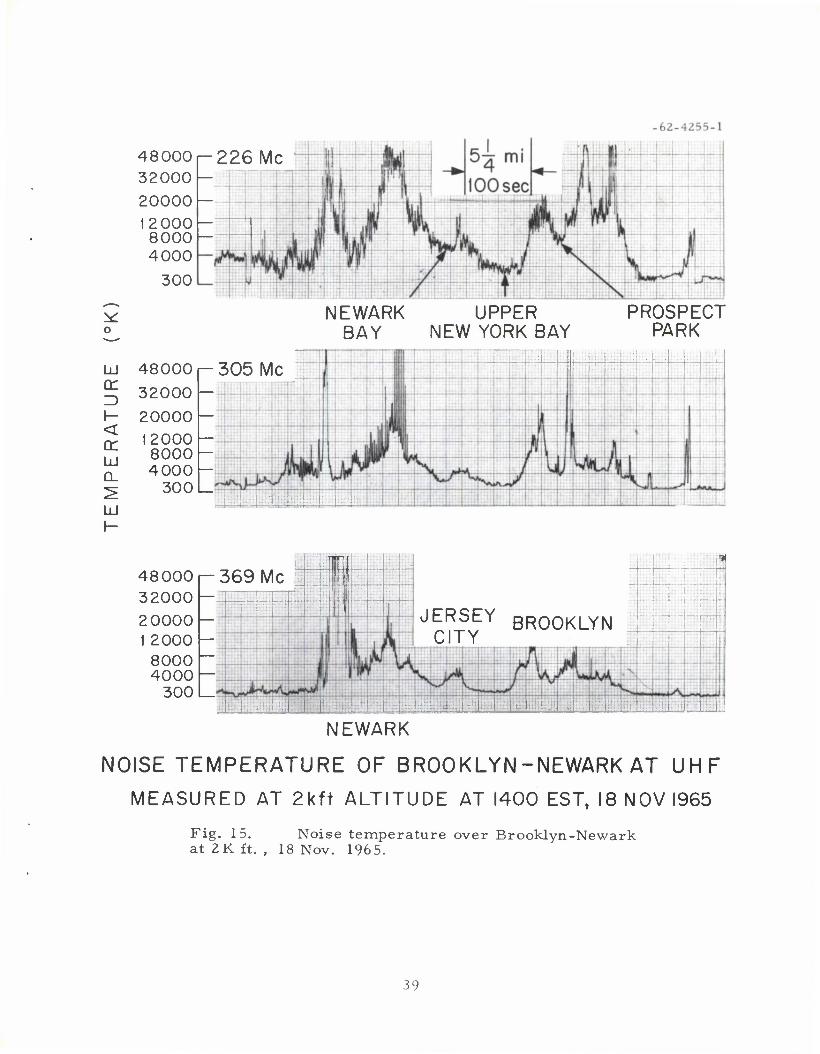
When flying at low altitudes greater detail of the power distribution becomes

apparent as is shown in Fig. 15.

Table II lists the noise temperature levels, T , measured over the

center of a number of U.S. cities. As seen from this table the only metro-

politan area that resulted in appreciably higher temperatures is New York.

The temperature levels recorded over Orlando and Jacksonville are lower

than the other cities listed due to the smaller angular sector these cities

occupied. To determine the average C of these cities the city limits would

have to be determined in order to compute the illumination angle \j) and

therefore I . However, it is seen from Fig. 11 that I saturates for illumina-

tion angles in excess of 60 . With the exception of Jacksonville and Orlando

all the data listed in Table II was obtained when J/J was very near 60 or

greater. Therefore the value of C for these cities is proportional to the

listed temperatures. In the case of Jacksonville and Orlando the illumination

angle was substantially less than 60 and therefore the corresponding I was

lower. This accounts for the lower temperatures listed for these two cities.

Data was taken during one night flight over the east coast cities. Un-

fortunately the weather was poor during this flight resulting in poor visibility

and P-static and consequently limiting the quantity and accuracy of the data.

However, the data did indicate a lower temperature level over the Baltimore-

12

Philadelphia-New York area. The levels were 3 to 7 db lower than previous

measurements made during normal working hours. These measurements were

taken between midnight and 2 A. M.

The frequency dependence of the noise temperature over a large number

of independent measurements was determined by selecting data points from

TABLE II

Noise Temperature Recorded on C-131 Over Eastern U. S. Cities

City Altitude Temperature (°K)

(Ft. ) 226. 2 MHz 305. 5 MH z 369. 2 MHz

Boston 8K 22,000 8,000 •*

Baltimore 18K 23,000 7,000 *

Jacksonville 14K 14,000 3,400 #

Miami (Cold) 18K 14,000 4,600 *

(Hot) 10K-18K 27,000 10,500 *

Orlando 9K 9,000 4, 000 2,200

Philadelphia 8K-18K 26,000 9,000 6,000

Brooklyn 8K-18K 60,000 19,000 9,500

Manhattan 8K-18K 75,000 30,000 16,000

""Accurate valui 2 s not obtained due to g] round RFI.

data runs at altitudes of 7. 5 K ft. and higher over all of the cities checked.

Points on the same run were chosen, separated sufficiently in time, to prevent

overlap of ground illumination. The ratio of the temperatures recorded at each

data point was computed and averaged. The result is:

13

T @ 305. 5 MHz

T & 226.2 MHz = * 31 (9)

a

T @ 369- 2 MHz

T 0 226.2 MHz = • 18 (10)

a

A total of 81 and 40 independent points were used in computing the ratios of

Eqs. (9) and (10) respectively.

In order to obtain a comparable relationship between the values of C

at the three test frequencies a relationship between the products G I at the

three frequencies must be determined. The data points chosen in evaluating

Eqs. (9) and (10) corresponded to points where 0 = -% + 20 . At 0 = 45 ,

1(0) at 369. 2 MHz is 1. 6 db greater then 1(0) at the two lower frequencies.

However the antenna gain G at 369. 2 MHz is 1-1/2 db lower than that at the

lower two frequencies. The product G I is therefore essentially the same at

all three frequencies at i/) =45 and will furthermore be assumed identical

for all the data points chosen. The values of C vs frequency are plotted in

Fig. 16 using the C computed for a ''hot" Miami at 305. 5 MHz and Eqs. (7)

and (9) and (10). Along with this data the often used values for Urban noise 12 published in the ITT handbook ' and converted to the same units is also

plotted. It is interesting to note that the average slope of the two curves is

similar but that the levels differ by 12. 5 to 14. 5 db. The difference in

magnitude is not surprising since the quantity being measured is not actually

the same, the ITT data representing the noise density experienced by a

receiver on the ground in the Urban area, in the middle of the random radiating

sources. Whereas C represents the effective noise density of the skyward

radiated power.

Antenna System Temperature

To determine analytically the effect of a city on the temperature of an

airborne antenna is a laborious procedure if one were to use Eq. (3) directly.

There are a couple of ways of circumventing this lengthy calculation however.

14

If the distance between the aircraft and the city is greater than the

largest dimension of the city and if the illumination pattern over the city is

fairly uniform a fair approximation of the antenna temperature can be made

by considering the city to be a point source at the city center. The effective

power radiated would then be the area of the city times the power density, C

from Fig. 16. The temperature is then calculated using Eq. (6).

If on the other hand the conditions above are not valid or if a more

precise calculation is desired a quick calculation can still be obtained by

partitioning the city into annular sectors that have a constant illumination

factor, D(9,0). Using Eq. (3) and the geometry of Fig. 17 we get for a sector

e2 T = _£ = X G.C f f ' cot9ded0

a kB i6ffzk J0, Je,

.2 sinQ?

J^- GC(0,- 0 ) In -r-J- (H) 16 TT 2 l sin9i

where G = G D(6,0)

= antenna gain over the sector a-b

From Fig. 17 we have:

0 _0 = _L. 2 1 r

o

sin 0

2 y<r0-^+h2

sin fl . = h (12) 1 , 2

(r +°) + h^ x o 2

15

T = a

\ 2 G C a

32 7TZk ro

(••^•c-^l In

o

G-IS-XTT) (13)

The sum of the temperatures from all the sections of the city defined

above will give a good approximation to Eq. (3). Equation (13) normalized to

\ G C is plotted in Fig. 18 as a function of b/r when a = b. Since the area of

the sector is a« b the independent variable is equivalent to the square root of

the sector area divided bv r .

A special limiting case occurs when flying over a city center with an

antenna that provides uniform illumination downward. Letting a = b = 2r we

define a triangular sector of a circle with radius 2r . There are IT such b o sectors in 360 . Therefore if the city is circular with radius 2r we get:

^-^^b+Q J (14)

The use of Fig. 18 to obtain a first approximation to the temperature

level expected is illustrated with the aid of data taken on the C-135 with the

upward looking blade antenna flying by the southern edge of Miami. The radio-

meter data is shown in Fig. 19. The flight path of the aircraft was south

easterly to a point south and slightly west of the city where a turn was executed

to the east, passing south of the city of Miami and crossing the coastline where

the antenna temperature drops below 300 K. Using Figs. 16 and 18 we can

compute the expected antenna temperature. A rough approximation of the Urban

area is to assume it to be a sector with a = b so that:

r = 12 mi.

b = Jin = 10. 8 mi

h = 6. 6 mi.

'. from Fig. 16

T = 300 \ZG C 10' o

= 1475 G (°K) o

18

16

During the turn the antenna declination angle corresponding to the city center

would be about 10 which corresponds to an antenna gain of approximately

+ 1 db I 1 db. The resultant expected additive temperature would be 1855 K.

As previously stated Miami appeared to exhibit temperature levels that

differed by 3 db depending upon the time of year. Since Fig. 18 is based upon

a "hot" Miami and the data of Fig. 19 was obtained in September we would

expect a temperature one-half that calculated. In addition, the background

noise temperature from the sky and earth of approximately 200 K has to be

added. The result is:

T expected = 1128°K ± 240° "cold"

2055°K ± 480° "hot"

T measured = 1800°K ± 180°

The discrepancy between the actual and expected temperature can be attributed

to the approximation of the city geometry, the fact that surrounding suburban

areas are not considered in the calculation, and that the value of C for Miami x varies by at least + 3 db as a function of the time of year.

After the turn was completed the aircraft flew south of the city in

level flight with a resultant measured temperature of approximately 1300 K.

Assuming a -1 db _ 1 db antenna gain in the direction of the city we get

T expected = 935°K - 190° "cold"

1670°K ± 380° "hot"

T measured = 1300°K - 130°

17

VI. CONCLUSIONS:

The noise level inherent to airborne UHF antenna systems has been

measured and characterized. The contributors to the overall noise level

have been identified and discussed with the exception of coherent RFI. The

results are summarized as follows:

1. Galactic and Thermal Earth Radiation: These sources contribute

a low level background noise level of 150 K to 300 K (low gain antenna).

Measurements were in general agreement with estimated values.

2. P-Static: This source of noise is negligible if modern static dis-

chargers are employed on the aircraft and care is taken in the antenna design.

3. Atmospherics: Noise levels measured due to lightning discharges

were 6 to 10 db lower than expected based upon extrapolated data in the litera-

ture. However, burst levels of several thousand degrees Kelvin are common

when within 10 to 20 miles of the discharge with peaks in the tens of thousands

of degrees. Burst rates of 20/min. were measured with typical burst width of

1/4 second.

4. City Noise: Analysis of data taken over cities in the Eastern

United States indicates that the city can be modeled electromagnetically as a

distributed aperture of random sources with uniform power density. The -18 - 18 2 power density was calculated to be 3 x 10 to 1 x 10 watts/m /Hz over

the UHF band. This value of power density was common to all cities during

the weekday with the exception of New York City which had a 5-6 db higher

level. Relations have been derived and curves plotted to compute antenna

temperature increase due to city noise based upon the metropolitan area

and range.

18

APPENDIX A

Measurement Equipment

The equipment used on the C-135 and C-131 was the same with the

exception of the antenna. A block diagram of the measurement equipment is

shown in Fig. A-l.

An ARI calibrated variable noise source was used during the measure-

ments for data calibration. The triplexer shown was fabricated from existing

coaxial cavities and was tuned to center frequencies of 226. 2 MHz, 305. 5 MHz

and 369. 2 MHz. The 3 db bandwidth of the triplexer was 1.6 to 1.7 MHz with

greater than 80 db rejection at Z. 10 MHz from center frequency. Low noise

(300 K) preamps were in each channel prior to the channel radiometer. The

radiometers shown were total power radiometers with a 2 msec integration

time and a 1. 2 MHz bandwidth. The outputs of the radiometers were amplified

and recorded on a 7 channel FM P. I. recorder. One of the 7 channels was

used for voice commentary, the remaining 6 used to record high and low

sensitivity signals from the 3 radiometers. A 2 channel T.I. chart recorder

was used on board for monitoring purpose. Likewise a tunable wideband CEI

receiver was used on the aircraft to monitor the three channels. Individual

line spectra in the 1. 2 MHz wide channels could be identified using the CEI

built-in spectral display.

The antenna used on the C-131 was a 2 dipole array mounted over a

flat ground plane, the combination mounted under the aircraft fuselage near

the aircraft tail. The average E and H plane half power beamwidth's at the

three operating frequencies were 42 and 112 respectively, the beam peak

facing earthward. The antenna was matched at the three operating frequencies

to a VSWR of less than 1. 5:1.

A standard military blade antenna (AT-256) was used on the C-135.

The antenna mounted on the top rear of the fuselage produced a donut-shaped

pattern roughly symmetrical about the vertical. The radiation was primarily

upward. An estimation of the percentage downward illumination was computed

19

using typical scaled-model pattern, produced by Boeing, of the antenna on a

C-135. The fore-aft elevation pattern differs from the broadside elevation

pattern due to the increased ground plane along the fuselage and the tail

assembly. The percentage of illumination vs. elevation angle is shown in

Fig. A-2, where the elevation pattern at broadside and fore-aft are considered

separately and as figures of revolution about the vertical and:

r0 2 K(!/)) = 27TG \ E (0 ) sin 0 d (/) (A-l) ° J0

An estimate of the total downward illumination by the average K(0) is shown

in Fig. A-2.

20

APPENDIX B

Antenna Illumination

In order to estimate C(9, 0) several approximations are made. From all

the data taken during this program, plus noise measurements made by others

on the ground, the noise density does not vary greatly within an urban area or

for that matter from city to city. C(9, 0 ) is therefore approximated by a con-

stant within the beam illuminated portion of the city and Eq. (3) of the text

can be written as:

0 9 \ r* 2. r> 2. T = —^— CG \ D(9,0) cot 9 d 9 d 0 (B-l)

a 16 ff^k J0, Je 1 1

Where the limits of integration correspond to the city limits and G (9) is

assumed to be unity. C can be computed once the value of the integral in B-l

is solved. However, the evaluation of this integral involves obtaining complete

contour radiation patterns and then use of a computer for the evaluation. This

effort is not consistent with the accuracy of the knowledge of the airborne

antenna radiation pattern or with the assumption of constant C. Fortunately,

a good analytical approximation to the radiation pattern can be made and with

some effort an analytical expression for the integral obtained.

The principal plane patterns of the test antenna have been measured. The

magnitude of the radiation pattern between the principal planes falls in between

these values forming an elliptically shaped beam. For cases where the ratio

of the principal axes of the "ellipse" is not too large, i. e. , for most of the

main beam a reasonable and convenient expression for the main beam radiation

pattern using the geometry of Fig. B-l is:

21

D(0,0) = E* (lj>) cos20 + E2 (»/)) sin 20 (B-2)

where

4,-l-e

E, (l/)) = normalized H-plane radiation pattern

2 E (0) = normalized E-plane pattern

The measured principal plane patterns are shown in Figs. B-2 and B-3 along

with simple functions that are good approximations to the E-plane and H-plane

pattern at all three frequencies. The integral of Eq. (B-l) can now be written

as:

f 7 f^(0) 2 2 pTp0(0) 2 2 1 = 4 \\ E. W>) cos 0tan0d 0 d 0 + 4 \ ' \ E (0) sin 0 tan0d0 d0 (B-3)

Jo Jo Jo Jo e

where

E2 (0) = cos 20 - J < 0 < J f = 305. 5 MHz and 226 MHz

= 0 \< |0|

77

• 975 "4" < 0 < J f = 369. 2 MHz (B-4)

E2e «/)) = cos2 2l/) -J < 0 < J

= 0 5<|0|

22

The beam contours obtained from the approximate analytic expression

at 305. 5 MHz are plotted in Fig. B-4 along with the measured contour obtained

from the principal plane and 45 plane patterns.

The limits of integration are defined by Fig. B-5. The component of I

due to E2 (0) at 226. 2 MHz and 305. 5 MHz is:

7T tan a

L = 4 \ \ sin \ji cos 0 cos 0 d 0 d 0 (B-5) h Jo ^0

where

tanli) o cos 0

TT Performing the integration we get for ij) < -j

\= TT tan2 0Q (l-sin0o) (B-6)

2 At 369. 2 MHz the E (l/;) contribution is:

-1 IT tan a

L = 4 V2" \ . 975 tani/jQ cos 20d I/J d 0 (B-7)

which results in Eq. B-8 for 0 < -^

r- 1 + sin l/) sin 0 -, = • 975 TT 1 n ^—2- - . - . °, (B-8) L cos UJ 1 + sinU) J v ' o o

23

ft The E-plane contribution to the integral I is constant when 0 < -j

2 77 since E ()/)) = 0 for !/) > -j. This constant is equal to:

7T 7T

" u " v

(B-9:

I = 4 \ \ cos 2 0 sin 0 tan 0 d 0 d 0 Jo Jo

= _ J (4 In . 707 + 1) = . 301 for lb > £ 4 x ro 4

7T When 0 is less than -j the integral I is the sum of two integrals defined by

the limits derived from Fig. B-5. These limits are:

-1 tan^o Sector I u) varies from 0 to tan -i—

cos 0

0 varies from 0 to cos (tan lb ) x ^o

7T Sector II 0 varies from 0 to j

-1 77 0 varies from cos (tan 0 ) to •*- (B-10)

The integral over the Sector II limits is relatively straightforward with

the result:

r -1* « -,1/2-, T -iQA, ff COS 0 & / 1 A2\ ^ -384L4 2 + 2 (1"5 > (B-12)

where 6 has been substituted for tani/j . Over Sector I the evaluation of ^o the I results in* e

*The integrals solved above are not simple due to the complexity of the limits. The solutions were obtained with the aid of integral tables in references 13 and 14.

24

I =6(1-6'') e I

1/2 ,2 .1/2

d+62)

26 . -1 f 1-6* Y •>« -1 c TfT tan \.—7TJ -26 COS 6

1+6'

1/2 + 26(l-62) [. 96 + . 1262 + . 10864 + .09166] (B-13)

where the last term of B-12 was obtained from the integration of the first 62

four terms of series expansion of 1 n (1 + ~— ). cos 0

In summary the value of I at the two lower frequencies:

I = 77 tan lb (1-sin )/> )+I +1 o ^o e. eJT

T7 0 < T ro 4

= 77tan lb (1- sinii ) + . 301 o o 5<*o<7 (B-14)

7T at 369. 2 MHz for 0 < i we get o 4

r 1 + sinl/) sinli) I=.97577^ L co >S0 + 1 +1 I+sinJp J e. e. (B-15)

77 The value of I was not evaluated at 369. 2 MHz for i/) < -j since the straight

line approximation for E results in an integral that is not solvable in closed n form plus the fact that most of the experimental data obtained and analyzed cor

77 responds to lb < -j.

I (0) is shown plotted in Fig. 11 of the text.

25

ACKNOWLEDGMENT

The author is indebted to D. Karp, R. V. Locke, and W. C. Provencher for their advice and efforts in the design and fabrication of the measurement equipment. The many flight hours logged by the above and S. B. Russell in accumulating the test data is also gratefully acknowledged.

Z6

REFERENCES

1. "Ground Terminal Noise Minimization Study - Final Report," No. WDL-TR 1972, Philco (18 January 1963), Contract No. AF 04 (695) -113, Sec. 2,3.

2. H. C. Ko, "The Distribution of Cosmic Radio Background Radiation," Proc. IRE, 46, 208 (Jan. 1958).

3. D. C. Hogg and W. W. Mumford, "The Effective Noise Temperature of the Sky," The Microwave Journal p. 80 (March I960).

4. S. N. C. Chen and W.H. Peake, "Apparent Temperatures of Smooth and Rough Terrain," IRE Transactions on Antennas and Propagation, p. 567 (Nov. 1961).

5. Handbook of Geophysics (The MacMillan Co. , New York, I960), p. 9-1.

6. Advances in Radio Research, 2, 121 (Academic Press, London, New York, 1964). _

7. R.L. Tanner and J.E. Nanevicz, "An Analysis of Corona-Generated Interference in Aircraft, " Proc. IEEE, 52, 44 (Jan. 1964).

8. J.E. Nanevicz and R.L. Tanner, "Some Techniques for the Elimination of Corona Discharge Noise in Aircraft Antennas," Proc. IEEE, 52, 53 (Jan. 1964).

9. "UHF Aircraft Satellite Relay Final Report of Flight Tests, " (Bendix Radio Div. , Baltimore, Md. , April 1965).

10. E.N.Skomal, "Distribution and Frequency Dependence of Unintentionally Generated Man-Made VHF/UHF Noise in Metropolitan Areas, IEEE Trans, on Electromagnetic Compatibility, Vol. EMC-7, 263 (Sept. 1965).

11. "Man-Made Noise" - Report to Technical Committee of the Advisory Committee for Land Mobile Radio Services from Working Group 3. (June 30, 1966).

12. "Reference Data for Radio Engineers, " 4th Edition (ITT, New York, 1964) p. 763.

13. H. B. Dwight, "Tables of Integrals and Other Mathematical Data, 4th Edition (MacMillan Co. , New York, 1961).

14. I.S. Gradshteyn and I. M. Ryzhik, "Tables of Integrals Series and Products," Academic Press (19657!

27

3-62-5783

Fig. 1.

200 300 500 1000

FREQUENCY (MHz)

Galactic temperature over a hemisphere.

28

3-62-5782

id

o' 10

\

\

X

10H ' \\

-XI

\ \ in

O 10-2 \ £ > \ \

L±J oc f

o io"3 - N\ CL

\ <

10"4

10"5

in"6 i ! I I I I I I

\

\ \

6 7 8

10 10 10

FREQUENCY(Hz)

Fig. 2. Mean ERP of atmospheric disturbance.

10

29

oo in

-A •

•

*

;

T

X

0>J

<£>

CM

1 1

•

o a n)

w

-a to o

•a h

n

ni u

00

o o o o OO

o o o o o o

(x») 3aniva3dW3i

30

N 00

S

~~5"^

* i <M J

S 4

I I I LJ_ o o o o o o o o o o O O O o -n

1

^

1

T

1

1

IK

o o o o o o o o o o o o

(M.) 3anivy3dW3i

3 8 *

i 1

y c n)

Xi

13 +J W

•rH

S-i

-a to o

i 6

13 OJ u

to

<L>

U

H

0£ • i-t

31

3"

X 2

o ro

*

1 :.2

Jt

i i i o o o o CM CD

u o

DC

43 GO

n)

0) 01

o a. to a) M

a>

£ o

• H XI

OX)

CO CM

X in

t CM

-.- r • . ,

dt

ro

J I

o o o o o o o o ro CD ^- —

„r

to

- !

|_L o o o o o o o o ^ - (D «

o o

:»o) 3yniva3dW3i

1—I

I

u a o

LO I

PU -a

co u oo

v 2

00

(Xo) 3yna.va3dW3i

32

3-62-5794

.. 2 cosy ,0 _, i dA = p T. dd dd> sino

Fig. 7. Antenna coordinate system.

3-62-5793

DISTRIBUTED SOURCE

Fig. 8. Geometry when distributed source is small compared to range.

3 3

TIME—•

Fig. 9. Radiometer response over Rte. 128 at 2,000 ft.

34

3-62-5790

5f 60 —

MARSH LAND

-30

CP

-150 -S

ATLANTIC OCEAN _l I I

MIAMI BEACH _

A-

CD"

70

90

70

50

CP

"O

CVJ CD

30

8 12 16 20

DISTANCE (mi)

24

Fig. 10. Angular boundary of Miami at 18,000 ft.

35

3-62-5791

2.0 - / /"

^, 1.5 369.2 MHz -^

-226.2 MHz H 1.0

AND 305.5 MHz

0.5

s' i i i i 1 1 1 1 0 10 20 30 40 50

<// ( deg)

60 70 80

Fig. 11. «*).

36

3-62-5825

Fig. 12. 17 Nov. 1965

6 8 10 12 14

DISTANCE (mi)

Power density profile of Miami @305. 5 MHz,

3-62-5784

o

UJ C£

H < UJ Q.

UJ

5000

4000-

3000 —

2000 —

1000

MEASURED DATA

\

ESTIMATED TEMPERATURE FOR CONSTANT Cv

± 8 12 16

DISTANCE (mi)

20 24

Fig, 13. Temperature profile of Miami @305. 5 MHz, measured traveling North over city at 18 K ft.

37

3-62-5826

cr

< LU O.

LU

28X103

24 x 10

3 20X10

16X103

12X103

/ "- \

8X103

; / \

3 4x10 / PHILADELPHIA \

0 i i i

DELAWARE RIVER

CITY JOHNSVILLE NAF- LIMIT WILLOW GROVE NAS

TIME-DISTANCE

Fig. 14. Temperature profile of Philadelphia at 226. 2 MHz, measured traveling North at 18K ft. , 18 Nov. 1965.

58

48000.- 226 Mc 32000 — 20000 — 12000 —" 8000 r- 4000

300

o

UJ cr

<

UJ

480001— 305 Mc 32000 20000 12000 8000 4000

300

NEWARK UPPER BAY NEW YORK BAY

PROSPECT PARK

!—\il

J^j^Y BROOKLYN

48000 r- 369 MC 32000 — 20000 - 1 2000 8000 4000 h

300

NEWARK

NOISE TEMPERATURE OF BROOKLYN-NEWARK AT UHF

MEASURED AT 2kft ALTITUDE AT I400 EST, 18 NOV I965

Fig. 15. Noise temperature over Brooklyn-Newark at 2K ft. , 18 Nov. 1965.

39

10 •16

3-62-5792

ITT DATA POWER DENSITY

MEASURED ON GROUND

£ 10"17

CM

•z.

Q

rr

o wiB a.

\ AIRBORNE MEASUREMENTS

EFFECTIVE GROUND POWER DENSITY

LINEAR POLARIZATION

10 19

200

Fig. 16.

X 500 300 400

FREQUENCY (MHz)

Effective city power density.

40

3-62-5786

Fig. 17. Sector geometry.

41

3-62-5785

5

0

00

b VA ro ro

Fig. 18. Antenna temperature vs. area illuminated.

42

3-62-5381-1

HEADING SE TURNING 12mi S OF MIAMI TO AN EASTERLY-

HEADING MEASURED ON C-135 AT 35kft ALTITUDE 14 SEP 1965

COAST LINE 12mi SOUTH

OF MIAM

40 mi NORTH OF MIAMI

40mi WEST OF PALM BEACH

1 mi 1 ' 300 °K

f-TIME REFERENCE

Fig. 19. Blade antenna temperature on C-135 at 226. 2 MHz, measured near Miami at 35Kft. , 14 Sept. 1965.

43

ANTENNA

V

COAX SWITCH

REFERENCE NOISE

SOURCE

TRIPLEXER

PREAMP

PREAMP

PREAMP

RADIOMETERS

226.2 MHz

305.5 MHz

369.2 MHz

TUNABLE WIDE-BAND RECEIVER

3-62-5779

TAPE RECORDER

CHART RECORDER

Fig. A-l. Measurement equipment.

44

3-62-5780

100

80

c o

a.

* 40 -

20

BROADSIDE PATTERN

AVERAGE

FORE-AFT PATTERN

-60 -40 -20 0 20 40 60 80

9 Fig. A-2. AT-256 illumination factor vs. elevation angle.

45

POLARIZATION

FLIGHT PATH

3-62-5788

CITY OUTLINE

GROUND ILLUMINATED

Fig. B-l.

SECTOR OF CITY ILLUMINATED

Mapping Geometry.

46

3-62-5778 3-62-5787

0 8

0.6

04 *>

0.4 -

0.2

1.0

0.8

0.6

j5- CVJ *.

0 4

0 2

369.2 MHz

305.5 MHz

Fig. B-2. Antenna E-plane patterns. Fig. B-3. Antenna H-plane patterns.

47

3-62-5789

180

ANALYTIC MEASURED

Fig. B-4. Contour plot of antenna pattern at 305. 5 MHz.

48

3-62-5781

FLIGHT PATH

TAN v^ COScjb

I LIMITS n

CITY EDGE

PATTERN LIMIT

T LIMITS e

(a) (b)

Fig. B-5. Limits of integration

49

DISTRIBUTION LIST

Director's Office

C. Robert Wieser Gerald P. Dinneen R. Joyce Harman Archives

Division 3

S.H.Dodd J. H. Chisholm J. Ruze

Division 4

J. Freedman

Division 6

W. E.Morrow P. Rosen

Group 6 1

L. J. Ricardi B. F. LaPage C. A. Lindberg

Group 62

I. L. Lebow P. R. Drouilhet K. L. Jordan B. E.Nichols

R. Alter J. H. Atchison S. L. Bernstein G. Blustein Y. Cho J. W. Craig W. R. Crowther J. D. Drinan H. E. Frachtman B.Gold

L. M. Goodman D.H. Hamilton H. H. Hoover A. H. Huntoon B. H. Hutchinson D.Karp R. V. Locke A. A. Mathiasen P.G. McHugh N. J. Morrisson F. Nagy C. W. Niessen G. Ploussios (6) F. G. Popp C. M. Rader C. A. Reveal S. B. Russell T.S.Seay I. Stiglitz P.Stylos J. Tierney D.K. Willim

E. J. Aho M. Alizeo W. D. Chapman P. Conrad E. Cross A. F. Dockrey C. M. Foundyller M.R.Goldberg T. E. Gunnison D. M.Hafford L.F.Hallowell J. M. Hart D. A. Hunt L. R. Isenberg M. Kraatz A. Lundin J. V. Moscillo W. C. Provencher R. J. Saliga T.Sarantos J. F. Siemasko R.S. Tringale D. C. Walden Group 62 Files

50

R. L. Bernier J. T. Butterworth J. V. Delsie R. E. Drapeau J. J. Drobot E. W. Edman P. R. Gendron A. J. Grennell A. V. Kesselhuth R. M. Kokoska A. L. Lipofsky M. D. MacAskill R. W.MacKnight L. F. Mullaney P. F. Murray A. W. Olson A. W. Pearson J. R. Ritchie S. Sawicki C. H. Symonds N. C. Vlahakis

Group 63

H. Sherman D. C. MacLellan P. Waldron M. Ash G.H.Ashley R.S.Berg A. Braga-Illa C. Burrowes R. W. Chick N. B. Childs J. B. Connolly M. C. Crocker A. I. Grayzel B. Howland C. L. Mack J. Max J. D. McCarron R. E. McMahon L. D. Michelove B. J. Moriarty D. M. Nathanson D. Parker J. L. Ryan F. W.Sarles W. G. Schmidt

V. J. Sferrino I. I. Shapiro R. L. Sicotte W. B. Smith D.. M. Snider A. G. Stanley D. Tang L. J. Travis N. R. Trudeau E. A. Vrablik

Group 64

P. E. Green H. W. Briscoe J. Capon L. T. Fleck P. L. Fleck E. Gehrels R. J. Greenfield E.J.Kelly R. J. Kolker R. T. Lacoss C. A. Wagner

Group 6 5

R. V. Wood R. G. Enticknap J. R. Brown J. P. Densler E. P. Edelson R. A. Guillette J.H.Helfrich I. Wigdor

Group 66

B.Reiffen J. U. Beusch T. J.Goblick B.E. White H.JL. Yudkin

51

Aerospace Corp. 2350 E. El Segundo Blvd. El Segundo, Calif.

Arrowsmith, E. B.

Aerospace Corporation San Bernardino Operations San Bernardino, California 92402

Skomal, E.S.

Airborne Instruments Laboratory Deer Park Long Island, New York 11729

Aylward, William R. , Jr. Sielman, Peter F.

Air Force Avionics Laboratory AVWC Wright-Patterson Air Force Base, Ohio, 45433

Boeing, Paul A.

Autonetics Division of North American Aviation, Inc. 3370 Miraloma Ave. Anaheim, Calif. 92803

Daniels, Robert L. Jaffe, Richard M. Reimherr, Robert N.

Avco Corp. Electronics Division Wilmington, Massachusetts 01887

Penndorf, Rudolf B.

Bendix Corporation Bendix Radio Division Baltimore, Maryland 21204

Betsill, Harry E. Guntner, Urban A. McComas, Arthur D.

Boeing Company P.O. Box 3707 Seattle, Washington 98124

Dalby, Thomas G. Freeman, Theodore K. Galloway, William C. Perkins, Leroy C. Streets, Rubert B. , Jr.

Boeing Company Airplane Division P.O. Box 707 Renton, Washington 98055

Axe, David C.

Booz-Allen Applied Research, Inc. 4733 Bethesda Ave. Bethesda, Maryland 20014

Canick, Paul M.

Collins Radio Co. Cedar Rapids, Iowa 52406

Bergemann, Gerald T. Loupee, Burton J.

Collins Radio Co. Dallas, Texas 75207

Cox, Robert T. Eckert, James E.

Communications Satellite Corp. 1900 L Street, N. W. Washington, D. C. 20036

Esch, Fred H. Martin, Edward J.

Metzger, Sidney

Communications Systems, Inc. Paramus, New Jersey

Dubbs, William M. Kandoian, Armig G. Lewinter, Sidney W.

52

Deco Electronics, Inc. 35 Cambridge Parkway Cambridge, Massachusetts

Welti, George R.

Deco Electronics, Inc. P.O. Box 551 Fort Evans Rd. Leesburg, Virginia

Edmunds, Francis E.

Defense Communications Agency Department of Defense Washington, D. C. 20305

Herr, Clyde W.

Harry Diamond Labs. Washington 25, D. C.

Salerno, James

Electronic Communications, Inc. 1501-72nd St. , North Box 12248 St. Petersburg, Florida 33733

Clark, Donald P. Ellett, James T. Ellington, Troy D. LaVean, Gilbert E.

Fairchild-Hiller Space Systems Division 1455 Research Blvd. Rockville, Maryland

Hoyer, Sigurd Kerr, John S.

Johnston, William A. , Jr.

Federal Communications Commission Washington, D. C. 20554

Skrivseth, Arnold G.

General Electric Company Missile and Space Division Valley Forge Space Technology Center Goddard Blvd. King of Prussia, Pennsylvania

Hagen, Donald L. Skolka, Kenneth M.

General Electric Company Defense Electronics Division 100 Plastics Ave. Pittsfield, Massachusetts

Haaland, Kenneth E.

General Electric Company Defense Programs Division 114 Waltham Street Lexington, Massachusetts

McClennan, John H.

General Electric Company 6901 Elmwood Ave. Philadelphia, Pennsylvania

Tenney, Raymond F.

Hazeltine Corporation Little Neck, New York 11362

Dunn, Bradley B. Regis, Robert

Hughes Aircraft Company 1901 W. Malvern Fullerton, California

Golden, Edward Hester, Robert G. Honnold, Vincent R. Sheridan, Edward W.

Hughes Aircraft Company Florence Avenue at Teale Culver City, California

Graves, Ross E. Weltin, Otto K.

5 3

International Business Machines Corp. 7220 Wisconsin Ave. Bethesda, Maryland

Blasbalg, Herman L. Haddad, Raymond A.

ITT Federal Laboratories 500 Washington Ave. Nutley, New Jersey 07110

Campbell, Donald R. Lyon, Zeon G. , Jr. Walker, James L.

Lockheed Missiles and Space Company P. O. Box 504 Sunnyvale, California

Briskin, Herbert B. Edwards, Lawrence K.

LTV Aerospace Corporation (A Subsidiary of Ling-Temco-Vought, Inc. 9314 Jefferson Blvd. P.O. Box 5907 Dallas, Texas 75222

Litton, Gail Thomas

Magnavox Research Laboratories 2829 Maricopa Street Torrance, California 90503

Cahn, Charles R. Judge, William J. Masterson, Steven A.

Martin Company P. O. Box 179 Denver, Colorado

Clausen, Reid H. Hardin, Robert H. Roberts, Alan F.

Martin Company P. O Box 5837 Orlando, Florida

Koppel, Herbert Prihar, David Y.

MITRE Corporation P.O. Box 208 Bedford, Massachusetts

Desrosiers, Albert J.

Motorola, Inc. Military Electronics Division Western Center 8201 East McDowell Road Scottsdale, Arizona

Engle, Kenneth J. Estes, Charles L. Krasin, Fred E.

) Motorola, Inc. Military Electronics Division 600 Main Street Waltham, Massachusetts

Kendall, Percy R.

North American Aviation, Inc. Space and Information Systems Div. 12214 Lakewood Blvd. Downey, California 90241

Hathaway, Robert N. Surrah, Gordon R. Wehner, Gilbert L.

Ohio State University 1314 Kinnear Road Columbus, Ohio 43212

Fouty, Robert A. Long, Ronald K. Zolnay, Stephen L.

54

Philco Corporation WDL Division 3825 Fabian Way Palo Alto, California

Bates, J. Fred Davies, Richard S. McClannan, Quinton B.

Radiation, Inc. Box 37 Melbourne, Florida

Barkman, Richard D. Seng, Frank G. Sissom, Alton W.

Radop Corporation of America Defense Electronic Products Camden, New Jersey

Feller, J. Solomon, K.

Radio Corporation of America Defense Electronic Products Moorestown, New Jersey

Bry, John C. Johnston, Thomas M. Sheridan, Thomas R.

Radio Corporation of America Defense Electronic Products Astro-Electronics Division P. O. Box 800 Princeton, New Jersey

Miller, Bernard P. Sherlock, Thomas M. Silverman, Donald

Raytheon Company 1415 Boston-Providence Turnpike Norwood, Massachusetts

Bickford, William J. Pontecorvo, Paul J. Tsao, Carson K. H.

Raytheon Company Space and Information Systems Div. 5Z8 Boston Post Road Sudbury, Massachusetts 01776

Gicca, Francis A. Trask, David B.

Sanders Associates, Inc. 95 Canal Street Nashua, New Hampshire 03060

Cullen, Francis P. Kingman, Gordon M.

Sylvania Electric Products, Inc. Wehrle Drive and Cayuga Road Williamsville, New York 14221

Diab, Khaled M. Gray, Donald J. Hyams, Henry C. Schlichter, Ernest S.

System Sciences Corporation 5718 Columbia Pike Falls Church, Virginia 22041

Burgess, John L. Cerva, Calvin H. Fruchter, Charles L Marsh, Edward N. Maxwell, David J.

Technical Communications Corp. 442 Marrett Road Lexington, Massachusetts 02173

Dayton, David S. Griffiths, Andrew S.

Smith, William H.

TRW Systems One Space Park Redondo Beach, California 90278

Littenberg, William

55

Westinghouse Electric Corp. Defense and Space Center Friendship International Airport Baltimore, Maryland 21203

Mongold, Guy E. Mueller, Edward J.

Robbins, Manuel A.

Whittaker Corporation 9229 Sunset Boulevard Los Angeles, California 90069

Cluster, Alvin P.

US AS C A U.S. Army Satellite Comm. Agency Fort Monmouth, New Jersey 07703

Chewey, Vincent C.

HQ. USAF

Naval Security Group Headquarters 3801 Nebraska Avenue Washington, D. C.

LCDR Angus D. McEachen, USN

Lt. Colonel H. A. Wilkes, USAF AFRDD Headquarters United States Air Force Washington, D. C. 20330

NAVY

Mr. John M. Comiskey U.S. Navy Underwater Sound

Laboratory Fort Trumbull

New London, Connecticut 06321

Department of the Navy Bureau of Naval Weapons Washington, D. C. 20360

Mr. Richard T. Shearer Cdr. Harold R. Gordinier, USN

Naval Electronics Systems Command 5805 Leesburg Pike Bailey's Crossroads, Virginia 22041

ODDR+E

RTD

Colonel Arthur W. Reese, USAF Office of Secretary of Defense Office of Director of Defense

Research and Engineering Washington, D. C. 20301

Mr. David Anderson Headquarters Research and

Technology Division (RTTC) Boiling Air Force Base, P. C. 20332

Mr. Mario J. Amico Mr. Joseph Awramik, Jr. Mr. Joseph J. Bogart Mr. Norman Horowitz Mr. Kenneth L. Nichols Mr. Harry M. Yakabe

Naval Communication Systems Hdqtrs. 5827 Columbia Pike Bailey's Crossroads, Virginia

Lt. Donald C. Gibson, USN

U.S. Naval Research Laboratory Washington, D. C. 20390

NAVY

Mr. Mr. Mr.

Theodore J. Altman Herman J. Wirth Robert W. Zeek

LCDR William R. Coffman, USN OPNAV Department of the Navy Washington, D. C. 20350

Cdr. A.K. Blough Department of the Navy Bureau of Ships Code 670G Washington, D. C.

56

UNCLASSIFIED Security Classification

DOCUMENT CONTROL DATA - R&D (Security classification of title, body of abstract and indexing annotation must be entered when the overall report is classified)

1. ORIGINATING ACTIVITY (Corporate author) 2a. REPORT SECURITY CLASSIFICATION

Lincoln Laboratory, M.I.T.

Unclassified 2b. GROUP

None 3. REPORT TITLE

Noise Temperature of Airborne Antennas at UHF

4. DESCRIPTIVE NOTES (Type ol report and inclusive dates)

Technical Note 5. AUTHOR(S) (Last name, first name, initial)

Ploussios, George

6. REPORT DATE 7a. TOTAL NO. OF PAGES 7b. NO. OF REFS

6 December 1966 62 14

8a CONTRACT OR GRANT NO.

AF 19(628)-5167 9a. ORIGINATOR'S REPORT NUMBER(S)

b PROJECT NO.

649L Technical Note 1966-5°

9b. OTHER REPORT NO(S) (Any other numbers that may be assigned this report)

d. ESD-TR-66-237

10. AVAILABILITY/LIMITATION NOTICES

Distribution of this document is unlimited.

1 1. SUPPLEMENTARY NOTES 12. SPONSORING MILITARY ACTIVITY

None Air Force Systems Command, USAF

13. ABSTRACT

Partial results of an experimental program to determine the electromagnetic noise environment at UHF on board an aircraft are presented. Contributors to an airborne receiver noise temperature including galactic noise, earth temperature. P-static. at- mospherics and industrial noise were measured and are discussed. A model of the in- dustrial noise is presented whereby the industrial area is considered as a uniformly dis- tributed source of independent radiators, the magnitude being the same for all cities measured with the exception of the New York City area.

RFI generated by on-board equipment and/or ground transmitters will be covered in a subsequent report.

14. KEY WORDS

airborne antennas precipitation static airborne receiver noise temperature atmospherics UHF antennas industrial noise galactic noise electromagnetic radiation thermal earth radiation

57 UNCLASSIFIED

Security Classification