Likelihood Ratio-Based Confidence Bands for Survival Functions Myles HOLLANDER, Ian W. McKEAGUE, and Jie YANG Thomas and Grunkemeier introduced a nonparametric likelihood ratio approach to confidence interval estimation of survival probabilities based on right-censored data. We construct simultaneous confidence bands using this approach. The boundaries of the bands are contained within [0, 1]. A procedure essentially equivalent to a bias correction is developed. The resulting increase in coverage accuracy is illustrated by an example and a simulation study. We look at various versions of log-likelihood ratio-based confidence bands and compare them to the Hall-Wellner band and Nair's equal precision band. We also construct likelihood ratio-based bands for cumulative hazard functions. KEY WORDS: Bias correction; Cumulative hazard rate; Kaplan-Meier estimator; Likelihood ratio statistic. 1. INTRODUCTION Thomas and Grunkemeier (1975)-TG hereafter- introduced a nonparametric likelihood ratio (LR) method for obtaining confidence intervals for a survival function So (t) at a given time point t. Our problem is to construct a simultaneous confidence band for So (t) over the time span of interest. We show that TG's pointwise confidence inter- vals can be adapted for this purpose. Our approach is based on their nonparametric LR statistic R(p,t) = sup{L(S): S(t) p, S E 61 (1) L(Sn)() where e is the family of all discrete survival functions sup- ported by the uncensored lifetimes, 0 < p < 1, Sn is the Kaplan-Meier estimator of So, and L is the likelihood func- tion L(S) fJ [S(Ti-) -S(Ti)] f 5(T), (2) U C where the The first product in (2) is taken over uncensored times, and the second product is taken over censored times. Kaplan and Meier (1958) showed that Sn, given by (13), is a non- parametric maximum likelihood estimator in the sense that it maximizes L without constraint. Li (1995a) showed that the LR defined by (1) is un- changed when e is replaced by the set of all survival func- tions on the interval [0, oc), so it represents a "full" LR. The TG asymptotic 100(1 - a)% confidence interval for So(t) is given by {p: - 2 log R (p, t) < x2 ,} (3) where 0 < oa < 1 and x2 a is the upper oa quantile of the chi-squared distribution with q degrees of freedom. A simultaneous large-sample confidence band for So can be obtained essentially by replacing p and x2 a in (3) by a survival function and an appropriate threshold determined by the data. We obtain a LR-based confidence band of the Myles Hollander is Distinguished Research Professor and Ian W. Mc- Keague is Professor and Chairman, Department of Statistics and Statis- tical Consulting Center, Florida State University, Tallahassee, FL 32306. Jie Yang is Research Associate, John S. Stafford Trading, Chicago, IL 60605. Ian McKeague acknowledges research support from National Sci- ence Foundation grant ATM-9417528. form B {S(t): -2 log R(S(t), t) < C2(t), t E [0, T]} (4) such that P(So E B) - 1- a, as n - oo, (5) where C(t) is given by (9) and T is the end of follow-up. The ratio L(S)/L(S,) may be regarded to be an "inverse distance" between S and Sn in the sense that the larger its value, the closer S is to Sn Thus B may be interpreted as a "neighborhood" of the Kaplan-Meier estimator Sn Note that for a fixed p, -2 log R(p, t) is the empirical LR for the upper p quantile and {to: -2 log R(p, to) < X2"} is the corresponding empirical likelihood confidence set. Owen (1988, 1990) used the empirical LR approach to construct confidence intervals for the mean, for a class of M estimates that includes quantiles, and for other differ- entiable statistical functionals in noncensored iid settings. This method has recently been further extended to deal with problems arising in linear regression, generalized lin- ear models, and other settings. It is advantageous to use empirical likelihood for several reasons. As noted by Hall and La Scala (1990), empirical confidence regions automat- ically reflect emphasis on the observed data set. This is seen in TG's confidence intervals for survival probabilities. Moreover, empirical likelihood regions are range preserv- ing and transformation respecting. That is, a LR based con- fidence interval for 0(O), a function of a parameter 0, is obtained by applying X to each value in the correspond- ing confidence interval for 0. This suggests that our LR confidence band for survival functions can be transformed to give a confidence band for the cumulative hazard func- tion A(t) = (S)(t) = fJt S(s-)-1 dF(s), t < T, where F = 1 - S. In Section 3 we show that this is a valid proce- dure. It was shown by TG and by Li (1995a) that L(S, t) -2logR(S(t),t) converges in distribution to chi-squared with 1 df for each fixed t E [0, T]. We consider the signed root-log-LR statistic ? 1997 American Statistical Association Journal of the American Statistical Association March 1997, Vol. 92, No. 437, Theory and Methods 215 This content downloaded from 156.145.72.10 on Mon, 07 Jan 2019 16:33:21 UTC All use subject to https://about.jstor.org/terms

Welcome message from author
This document is posted to help you gain knowledge. Please leave a comment to let me know what you think about it! Share it to your friends and learn new things together.
Transcript
Likelihood Ratio-Based Confidence Bands for
Survival Functions Myles HOLLANDER, Ian W. McKEAGUE, and Jie YANG
Thomas and Grunkemeier introduced a nonparametric likelihood ratio approach to confidence interval estimation of survival probabilities based on right-censored data. We construct simultaneous confidence bands using this approach. The boundaries of
the bands are contained within [0, 1]. A procedure essentially equivalent to a bias correction is developed. The resulting increase in coverage accuracy is illustrated by an example and a simulation study. We look at various versions of log-likelihood ratio-based confidence bands and compare them to the Hall-Wellner band and Nair's equal precision band. We also construct likelihood ratio-based bands for cumulative hazard functions.
KEY WORDS: Bias correction; Cumulative hazard rate; Kaplan-Meier estimator; Likelihood ratio statistic.
1. INTRODUCTION
Thomas and Grunkemeier (1975)-TG hereafter-
introduced a nonparametric likelihood ratio (LR) method
for obtaining confidence intervals for a survival function
So (t) at a given time point t. Our problem is to construct a simultaneous confidence band for So (t) over the time span
of interest. We show that TG's pointwise confidence inter-
vals can be adapted for this purpose. Our approach is based
on their nonparametric LR statistic
R(p,t) = sup{L(S): S(t) p, S E 61 (1) L(Sn)()
where e is the family of all discrete survival functions sup-
ported by the uncensored lifetimes, 0 < p < 1, Sn is the Kaplan-Meier estimator of So, and L is the likelihood func- tion
L(S) fJ [S(Ti-) -S(Ti)] f 5(T), (2) U C
where the Ti are the possibly right-censored failure times. The first product in (2) is taken over uncensored times, and
the second product is taken over censored times. Kaplan
and Meier (1958) showed that Sn, given by (13), is a non- parametric maximum likelihood estimator in the sense that it maximizes L without constraint.
Li (1995a) showed that the LR defined by (1) is un-
changed when e is replaced by the set of all survival func- tions on the interval [0, oc), so it represents a "full" LR. The TG asymptotic 100(1 - a)% confidence interval for So(t) is given by
{p: - 2 log R (p, t) < x2 ,} (3) where 0 < oa < 1 and x2 a is the upper oa quantile of the chi-squared distribution with q degrees of freedom.
A simultaneous large-sample confidence band for So can
be obtained essentially by replacing p and x2 a in (3) by a survival function and an appropriate threshold determined by the data. We obtain a LR-based confidence band of the
Myles Hollander is Distinguished Research Professor and Ian W. Mc- Keague is Professor and Chairman, Department of Statistics and Statis- tical Consulting Center, Florida State University, Tallahassee, FL 32306. Jie Yang is Research Associate, John S. Stafford Trading, Chicago, IL
60605. Ian McKeague acknowledges research support from National Sci- ence Foundation grant ATM-9417528.
form
B {S(t): -2 log R(S(t), t) < C2(t), t E [0, T]} (4)
such that
P(So E B) - 1- a, as n - oo, (5)
where C(t) is given by (9) and T is the end of follow-up.
The ratio L(S)/L(S,) may be regarded to be an "inverse distance" between S and Sn in the sense that the larger its
value, the closer S is to Sn Thus B may be interpreted as
a "neighborhood" of the Kaplan-Meier estimator Sn
Note that for a fixed p, -2 log R(p, t) is the empirical LR
for the upper p quantile and {to: -2 log R(p, to) < X2"} is the corresponding empirical likelihood confidence set.
Owen (1988, 1990) used the empirical LR approach to construct confidence intervals for the mean, for a class of M estimates that includes quantiles, and for other differ-
entiable statistical functionals in noncensored iid settings.
This method has recently been further extended to deal
with problems arising in linear regression, generalized lin-
ear models, and other settings. It is advantageous to use empirical likelihood for several reasons. As noted by Hall
and La Scala (1990), empirical confidence regions automat- ically reflect emphasis on the observed data set. This is
seen in TG's confidence intervals for survival probabilities.
Moreover, empirical likelihood regions are range preserv- ing and transformation respecting. That is, a LR based con-
fidence interval for 0(O), a function of a parameter 0, is obtained by applying X to each value in the correspond- ing confidence interval for 0. This suggests that our LR confidence band for survival functions can be transformed
to give a confidence band for the cumulative hazard func-
tion A(t) = (S)(t) = fJt S(s-)-1 dF(s), t < T, where F = 1 - S. In Section 3 we show that this is a valid proce- dure.
It was shown by TG and by Li (1995a) that L(S, t) -2logR(S(t),t) converges in distribution to chi-squared with 1 df for each fixed t E [0, T]. We consider the signed root-log-LR statistic
? 1997 American Statistical Association Journal of the American Statistical Association
March 1997, Vol. 92, No. 437, Theory and Methods
215
This content downloaded from 156.145.72.10 on Mon, 07 Jan 2019 16:33:21 UTCAll use subject to https://about.jstor.org/terms
216 Journal of the American Statistical Association, March 1997
W(S,t)= sgn(S,(t) - S(t)) C(S,t) (6)
and show that the process {f((t)W(So,t),t c [0,T]} con- verges weakly to a mean zero Gaussian martingale with variance that is consistently estimated by -2(t) = &-(t), given by (17). The limiting process can be transformed to
a Brownian bridge BO, so that
sup 3.(t)W(So,t) p> sup IB0(x)l, (7) tC[O,T] 1 + c2 (t) xG[O,d]
where d is consistently estimated by d (2 (T)/ {1 + 52(T)} (see Andersen, Borgan, Gill, & Keiding 1993, Chap. IV, Sec. 1.3). This result is used to construct our
asymptotic 100(1 - oa)% confidence band for So:
t3 = {s(t): ( ) (S (t) |< Kq,o(d) ,t C [0, T] 1?8&2 (t) - qc)C,J
= {S(t): JW(S(t), t)j < C(t), t C [?' T]}' (8)
where
C(t) - Kq,o(d) + 82(t) t > O, (9)
C(O) = 0, and Kq,o(d) is the upper oa quantile of the dis- tribution of SUPxc[O,d] IB0(x)l. An explicit formula for the distribution was given by Hall and Wellner (1980, eq. 2.9). (Some critical values for different choices of oa can also be found in that work.) Because -2(t) is a step function, C(t) is also a step function, so the confidence band can be com-
puted in finitely many steps (see Sec. 2). As we have seen in (4), the confidence band can be interpreted as a class of survival functions. The boundaries of the band are re-
stricted by [0, 1], which is especially appealing for survival probabilities near 0 or 1.
Simultaneous confidence bands for the survival function based on the limiting distribution of the Kaplan-Meier esti- mator, as obtained by Efron (1967) and Breslow and Crow- ley (1974), have been available since the work of Gillespie and Fisher (1979). The most commonly used confidence band is that due to Hall and Wellner (1980), HW here- after. They proposed the asymptotic 100(1 - a)% confi- dence band
Sn (t) ? n- 1/2Sn (t)Kq,o (d) (1 + ?2 (t)), t C [0, T]. (10)
This band reduces to the well-known Kolmogorov band for uncensored survival data. Another commonly used confi- dence band is the equal precision band (Nair 1984)
1/2e &2~~ (3(t) Sn(t)?n-1/2e cSn(t)c3(t), Vt: a< 2 (2t)_ b. (11)
Here ec, = ec, (a, b) satisfies
{uC[Pxb][U(l- ie} l-1a. To construct this band, one must choose values of a and
b. Some critical values for different choices of ae and a= 1 - b were given by Nair (1984, tab. 2). The equal preci-
sion (EP) band has the same form as the standard asymp-
totic pointwise confidence intervals for So(t): Si,(t) ?
Z./2n-1/2Sn(t)&(t). When there is no censoring, the band reduces to
Sn(t) ? eCo, [nt(-S()]n (12)
Nair's simulations indicate that the Renyi-type band de-
scribed by Gill (1980) is generally inferior to the other bands, and thus we have excluded it from our numerical study.
A shortcoming of the usual HW and the EP confidence
bands is that they may contain values outside [0, 1]. One way to overcome this problem is to use the log-log transfor-
mation, g(x) = log(- log x), or the arcsine transformation, g(x) = arcsinjix, suggested, respectively, by Kalbfleisch and Prentice (1980) and TG. The latter is variance stabi- lizing for the situation with no censoring. Our LR band
does not require such an ad hoc procedure. Nevertheless, it is possible and advantageous to consider transformations to improve the approximation to the asymptotic distribu- tion. With the transformation that Nair used to obtain his EP band, we can have an LR band B = {S(t): L(S,t) < e2 (a, b)}. Essentially, this takes the same form as TG's con- fidence interval in (3), except that the threshold C2(t) is replaced by a fixed critical value larger than x2 .
We recommend the LR confidence bands because, as we show herein (a) they have satisfactory coverage accuracy,
(b) their boundaries are naturally contained in [0, 1], and (c) they are transformation preserving.
The LR approach is useful in other incomplete data problems in survival analysis. For example, Li, Hollander, McKeague, and Yang (1996) found confidence bands for the quantile function, Li (1995b) gave confidence intervals for survival probabilities based on truncated data, and Murphy (1995) gave pointwise confidence intervals for the survival function and the cumulative hazard function.
In Section 2 we introduce our two LR confidence bands and develop the requisite asymptotic theory. The second of these bands corrects for possible "small-sample" bias in the first band. We discuss LR confidence bands for cumulative hazard functions in Section 3. In Section 4 we illustrate our survival function bands in examples and report the re-
sults of a simulation study. We compare our LR bands to the Hall-Wellner band and to Nair's equal precision band, including their arcsin and log-log transformed bands. We
present proofs in the Appendix.
2. CONSTRUCTION OF CONFIDENCE BANDS
Our basic LR confidence band for the survival function
is studied in Section 2.1. The bias correction is discussed in Section 2.2.
2.1 Construction of Basic Likelihood Ratio Bands
Let X1, . .., Xn be iid survival times with survival func- tion S, and let Ci, ... ., Cn be iid censoring times with sur- vival function Sc, independent of the Xis We observe
This content downloaded from 156.145.72.10 on Mon, 07 Jan 2019 16:33:21 UTCAll use subject to https://about.jstor.org/terms
Hollander, McKeague, and Yang: Confidence Bands for Survival Functions 217
Table 1. The 1994 JASA Time-to-First-Review Data (Time in Days)
Ti 8i T1 8i Ti 8i Ti 8i T1 8i Ti 8i T1 8i T1 8i T1 6, Ti 6, T1 8i
214 1 201 1 28 1 252 0 118 1 187 0 28 1 28 1 76 1 56 0 28 0 184 1 274 1 287 0 96 1 33 1 152 1 21 1 118 0 18 1 21 1 27 0 150 1 265 1 195 1 175 1 69 1 46 1 1 1 40 1 88 0 55 0 27 0 70 1 120 1 86 1 54 1 133 1 103 1 0 1 6 1 85 0 55 0 25 0 16 1 141 1 137 1 167 1 126 1 37 1 144 0 91 1 85 0 54 0 25 0 141 1 48 1 74 1 150 1 84 1 170 1 144 0 34 1 85 0 18 1 22 0 210 1 204 1 71 1 219 1 197 1 64 1 140 0 21 1 20 1 54 0 22 0 132 1 312 0 140 1 86 1 85 1 182 0 14 1 1 1 83 0 53 0 21 0 30 1 220 1 22 1 1 1 15 1 180 0 0 1 111 0 82 0 50 0 21 0 204 1 188 1 120 1 111 1 206 1 176 0 27 1 111 0 81 0 50 0 15 0 84 1 84 1 176 1 128 1 125 1 175 0 23 1 1 1 81 0 1 1 15 0 36 1 84 1 181 1 178 1 57 1 64 1 126 1 48 1 11 1 15 1 15 0 38 1 215 1 155 1 40 1 181 1 42 1 139 0 110 0 77 0 50 0 1 1 69 1 33 1 74 1 131 1 215 0 175 0 55 1 47 1 77 0 47 0 1 1 33 1 55 1 29 1 20 1 3 1 149 1 137 0 68 1 70 1 47 0 14 0 49 1 140 1 100 1 220 1 13 1 158 1 114 1 74 1 74 0 46 0 12 0 203 1 147 1 195 1 84 1 175 1 169 0 56 1 98 1 71 0 16 1 12 0 203 1 41 1 127 1 32 1 37 1 169 0 124 1 105 0 23 1 43 0 12 0 218 1 94 1 34 1 95 1 182 1 22 0 121 1 104 0 28 1 43 0 8 0 267 1 292 1 177 1 188 1 210 0 168 0 1 1 104 0 70 0 18 1 8 0 99 1 131 1 150 1 115 1 92 1 157 1 27 1 103 0 44 1 43 0 8 0 21 1 221 1 265 0 238 0 208 0 89 1 130 0 90 1 69 0 42 0 8 0 78 1 39 1 174 1 1 1 30 1 165 1 130 0 98 0 68 0 42 0 7 0 150 1 3 1 104 1 187 1 28 1 14 1 130 0 98 0 67 0 40 0 7 0 237 1 16 1 203 1 125 1 168 1 161 0 127 0 98 0 64 1 0 1 7 0 91 1 129 1 109 1 110 1 202 0 161 0 100 1 97 0 30 1 12 1 7 0 21 1 210 1 217 1 32 1 114 1 159 0 126 0 96 1 41 1 39 0 6 0 224 1 240 1 238 1 32 1 105 1 91 1 126 0 97 0 62 0 35 0 5 0 126 1 141 1 210 1 228 1 196 0 146 1 28 1 18 1 61 0 35 0 5 0 167 1 231 1 22 1 80 1 195 0 159 0 125 0 96 0 20 1 35 0 4 0 105 1 119 1 148 1 64 1 114 1 134 1 125 0 92 0 57 0 30 1 1 0 146 1 291 0 142 1 231 0 75 1 13 1 125 0 91 0 57 0 35 0 1 0 50 1 199 1 126 1 64 1 194 0 159 0 95 1 91 0 57 0 34 0 28 1 67 1 220 1 228 0 143 1 18 1 95 1 91 0 57 0 34 0 288 1 263 1 145 1 18 1 106 1 155 0 123 0 31 1 57 0 34 0 37 1 155 1 21 1 55 1 128 1 154 0 123 0 27 1 57 0 33 0 18 1 189 1 256 0 154 1 200 0 124 1 123 0 83 1 42 1 33 0 113 1 0 1 253 0 139 1 129 1 73 1 109 1 33 1 57 0 29 1 22 1 209 1 22 1 91 1 138 1 51 1 119 0 11 1 57 0 28 0 234 1 223 1 80 1 196 1 152 1 21 1 6 1 88 0 57 1 27 0
('l l v1 ... )v ('ln) 6n)7,) where Ti = min(Xi, C>i), 6i = l (Xi < Ci), and I(E) is the indicator of the event E. We reserve the notation So for the true underlying survival function.
We introduce some notation as follows. Let Y(t)
n I(Ti > t) be the number of individuals at risk just before time t, let N(t) = I (Ti < t, 6= 1) be the counting process that records the uncensored failures, and
let AN(s) = N(s) - N(s-). The Kaplan-Meier estimator of SO is
Sn(t) =fl(1 - AN(s), 0 < t < XI), (13) S<t Y(S)
where AN(s)/Y(s) is defined to be 0 whenever Y(s)
0. Due to tail instability of the Kaplan-Meier estimator, simultaneous confidence bands can be obtained only on an
interval [0, T], where H(T) > 0 and H(t) = So (t)Sc (t). We fix such a T from now on.
We show that W(So, t) converges weakly to a Gaussian process; that is the basic result for constructing our confi-
dence band. To that end, recall from TG that
L(S, t) = -2 , { [Y(s) - AN(s)] s<t
x log (1 ? Y(s) -AN(s)) }
+ 2 {Y(s) log (1 + f))} (14) S<t YS
where An = An (S, t) satisfies
i (1 _ AN(s) )=S(t). (15) S<t
To obtain an explicit expression for W, it is necessary to solve (15) for An. An explicit solution is not possible, but a suitable approximation for L(S, t) will suffice. Thus
our first step is to find an approximation for A,. For future reference, we define
dA(s) 052(t) = JOS {A(,) t E [0) T]) r = 0,1, ... ,4)
(16)
This content downloaded from 156.145.72.10 on Mon, 07 Jan 2019 16:33:21 UTCAll use subject to https://about.jstor.org/terms

218 Journal of the American Statistical Association, March 1997
C(a (b)
co o
0 5 1015202530 =35 0 5 0 5 0 5 0 5
o( (d )
106- 16 ~~~~~~~~~~~~~2 L-j
g no!)srd W ndE Bnd (asedLies.(a) L n W (b) LC n P c R n W d R n P
a.
C)~~~~~~~~~~~~~~~~~~~~C
0~..0 2010102020 0 5 0101 0 5 0 5
0 0D
(L (L~~~~() d
Fiue1 EtmtdPrbblt (oi ie)ta FrtRvewo AA aucit ae one hnt as ih 5 RBnd Dte Lies an WadE ad Dse ies.()L' n W b R;ad P C R n W()R,nE
and a2 (t) = g2 (t). The asymptotic variance of the Kaplan-
Meier estimator at time t is u2(t)S02(t). It is easy to show that
&r2(= nr+l [ I(Y > 0) dN (17) r ~ J~yr+l(Y - AN) is a uniformly consistent estimator of a 2 (t), t E [0, T]. Also, denote &2(t) = &2(t) and
K(S, t) = log Sn(t) - log S(t). (18)
Theorem 2.1. The signed root-log-LR of L?(S, t) has an asymptotic expansion
W(S t) = y?K(S,t) _ ? &1K2(S,t) a 3
+ 36\J (16&4 - 9&2&f2)K3(S, t) + ? (n-3/2)
where the dependence of (Jr on t has been suppressed. This and all subsequent expansions involving Op terms hold uniformly in t over the interval [0, T].
Remark 2.]. To find the asymptotic distribution of W, we need only the first two terms of the foregoing expansion.
The two-term expansion of W is
W(S, t) = )K(S,t) _ . &1K2(S,t) ?O0(n71) (19) a" 3 &
To derive the limiting distribution of W, we need a lemma. Lemma 2.1. y?K(So, t) converges weakly to U(t) in
D[O, T] as n -+ ox, where U(t) is a Gaussian martingale with mean zero and variance function a2(t).
Theorem 2.2. &(t)W(So,t) converges weakly to U(t) in D[0, T], where U(t) is defined in Lemma 2.1.
It follows from Theorem 2.2 that
8(t)W(So0t) , U(t) (20) 1 + &2(t) 1 ? o2(t)
in D[0,T], so
sup & (t) W(So t)D sup IBo(x) (21) tE[O,r] 1 ? O"2(t) XE[O,d]
where
d- l+ (2(T) d = - - ~~~~~(22)
This content downloaded from 156.145.72.10 on Mon, 07 Jan 2019 16:33:21 UTCAll use subject to https://about.jstor.org/terms
Hollander, McKeague, and Yang: Confidence Bands for Survival Functions 219
O 0
co=
0 50 100 150 200 250 300 350 0 50 100 150 200 250 300 350
Time (days) Time (days)
(a) (b)
flCO
26:~~~~~~~~~~~~~~~~~~~~~~~2c
a. re
0 c
0 50 100 150 200 250 300 350 0 50 100 150 200 250 300 350
Time (days) Time (days)
(c) (d)
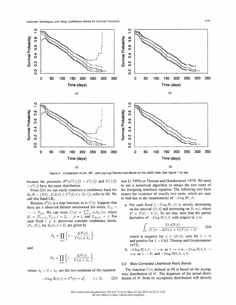
Figure 2. Comparison of LR-, EP-, and Log-Logl-Transformed Bands for the JASA Data. See Figure 1 for key.
because the processes B0{f2(.)/[1 + a2(.)]} and U(.)/[1 + a2 (.)] have the same distribution.
From (21) we can easily construct a confidence band for So 13 {S(t): C(S, t) < C2 (t), t E [O, T ] }; refer to (8). We call this band LR1.
Because P2(t) is a step function, so is C(t). Suppose that there are k observed distinct uncensored life times, T(i) <
< T(k). We can write C(s) = Zk=l aiIE%(S), where
Ei = [T(i - )I T(i) )= 2,... Ik + 1, and T(k+1) = T. For each fixed i < k, piecewise constant confidence limits, [PL, PU], for S0(t), t E Ei are given by
PL = J {1- Y (s)?L} S<t Ys)+A
and
S<t { Y(S) + Au }
where AL < 0 < Au are the two solutions of the equation
-2logR(A,t) = C2(t) = a 2, t E Ei (23)
(see Li 1995a or Thomas and Grunkemeier 1975). We need to use a numerical algorithm to obtain the two roots of the foregoing nonlinear equation. The following two facts ensure the existence of exactly two roots, which are easy to find due to the monotonicity of -2 log R(., t):
a. For each fixed t, -2 log R(, t) is strictly decreasing on the interval (D, 0] and increasing on [0, oc), where D = N(t) - Y(t). To see this, note that the partial derivative of -2 log R(A, t) with respect to A is
(Y(s)- AN(s) + A)(Y(s) + A)' (24) which is negative for A E (D, 0), zero for A = 0, and positive for A > 0 (cf. Thomas and Grunkenmeier 1975).
b. -2logR(A,t) -* +oo as A -* +oo,-2logR(A,t) +oo as A -* D, and -2 log R(0, t) = 0.
2.2 Bias-Corrected Likelihood Ratio Bands
The function C(t) defined in (9) is based on the asymp- totic distribution of W. The departure of the actual distri- bution of W from its asymptotic distribution will directly
This content downloaded from 156.145.72.10 on Mon, 07 Jan 2019 16:33:21 UTCAll use subject to https://about.jstor.org/terms
220 Journal of the American Statistical Association, March 1997
co co
2= 0
cU C
0 50 100 150 200 250 300 350 0 50 100 150 200 250 300 350
Time (days) Time (days)
(a) (b)
20 co Z. -5
0~~~~~~~~~~~~~~~~~~c
o o
0 50 100 150 200 250 300 350 0 50 100 150 200 250 300 350
Time (days) Time (days)
(c) (d)
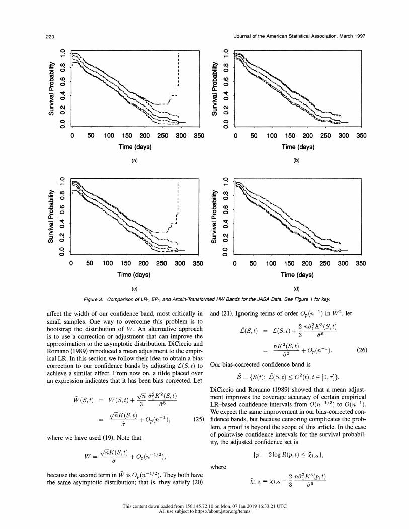
FiguJre 3. Comparison of LR-, EP-, and Arcsin- Transformed HW Bands for the JASA Data. See Figure 1 for key.
affect the width of our confidence band, most critically in small samples. One way to overcome this problem is to bootstrap the distribution of W. An alternative approach is to use a correction or adjustment that can improve the approximation to the asymptotic distribution. DiCiccio and Romano (1989) introduced a mean adjustment to the empir- ical LR. In this section we follow their idea to obtain a bias correction to our confidence bands by adjusting L(S, t) to achieve a similar effect. From now on, a tilde placed over
an expression indicates that it has been bias corrected. Let
W(S,t) = (S t) + N/I 1 -5 3 a
- \/?K(S,t) + (n-l) (25)
where we have used (19). Note that
W - V/TK(S, t) + op(n- 1/2
because the second term in W is Op(n 1/2). They both have the same asymptotic distribution; that is, they satisfy (20)
and (21). Ignoring terms of order Op(n-1) in 12, let
2 r8~3 (S, t) ?(S,t) = ?(S, t) + 2 n 8.6l K
nK2 (S, t) + Op(n-1) . (26) 8&2
Our bias-corrected confidence band is
B = {S(t): ?(S,t) < C2(t),t C [O,I_]}.
DiCiccio and Romano (1989) showed that a mean adjust- ment improves the coverage accuracy of certain empirical LR-based confidence intervals from Q(n-1/2) to 0(n-1). We expect the same improvement in our bias-corrected con- fidence bands, but because censoring complicates the prob- lem, a proof is beyond the scope of this article. In the case of pointwise confidence intervals for the survival probabil- ity, the adjusted confidence set is
{p: -2 log R(p, t) < X,}
where
-1,a = ~ - 2 n8.2K3 (p, t) X~1,a = X1,-a 8.6
This content downloaded from 156.145.72.10 on Mon, 07 Jan 2019 16:33:21 UTCAll use subject to https://about.jstor.org/terms
Hollander, McKeague, and Yang: Confidence Bands for Survival Functions 221
co co CU
n CD U0C 2 0 2 0
(a) ~ ~ ~ ~ ~ / 0b
i3 ?i \, < gN
o o 0 ~~~~~~~~0
0 50 100 150 200 250 300 350 0 50 100 150 200 250 300 350
Time (days) Time (days)
(a) (b)
ao ~co FL0
I ,zl.he ie) ()L2(ote ie)an R dshdlns; d R dffdlns adL2(ase ie)
20 2o
cm ~ ~ ~ ~ ~ ~ ~ ~ ~ ~ '
0 50 100 150 200 250 300 350 0 50 100 150 200 250 300 350
Time (days) Time (days)
(c) (d)
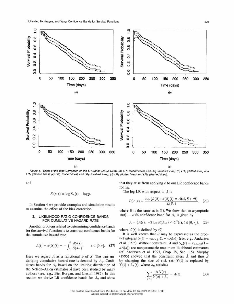
Figure 4. Effect of the Bias Correction on the LR Bands (JASA Data). (a) LRc, (dotted lines) and LR2c (dashed lines); (b) LRc, (dotted fines) and LR, (dashed fines); (c) LR2c (dotted lines) and LR2 (dashed lines); (d) LR, (dotted lines) and LR2 (dashed fines).
and
K(p, t) = log Sn (t) - log p.
In Section 4 we provide examples and simulation results to examine the effect of the bias correction.
3. LIKELIHOOD RATIO CONFIDENCE BANDS FOR CUMULATIVE HAZARD RATE
Another problem related to determining confidence bands for the survival function is to construct confidence bands for the cumulative hazard rate
A(t) = (S)(t) = -) t e [O] (27)
Here we regard A as a functional X of S. The true un-
derlying cumulative hazard rate is denoted by Ao. Confi- dence bands for Ao based on the limiting distribution of the Nelson-Aalen estimator A have been studied by many authors (see, e.g., Bie, Borgan, and Liest0l 1987). In this section we derive LR confidence bands for Ao and show
that they arise from applying 0 to our LR confidence bands for So.
The log-LR with respect to A is
sup{L(S): 0(S)(t) = A(t),S E E} ( R(A, t) = L(-),(28)
where E is the same as in (1). We show that an asymptotic 100(1 - a)% confidence band for Ao is given by
A = {A(t): -2 log R(A, t) < C2(t), t E [O,]}, (29)
where C(t) is defined by (9). It is well known that S may be expressed as the prod-
uct integral S(t) = 7ro<s<t(l - dA(s)) (see, e.g., Andersen
et al. 1993). Without constraint, A and Sn(t) = 70<8<t(i - dA(s)) are nonparametric maximum likelihood estimators (cf. Andersen et al. 1993, Chap. IV, Sec. 1.5). Murphy (1995) showed that the constraint alters A and thus S by changing the size of risk set: Y(t) is replaced by Y(t) + An (t), where An satisfies
ZE YN(s) =A(t). (30) S<t
This content downloaded from 156.145.72.10 on Mon, 07 Jan 2019 16:33:21 UTCAll use subject to https://about.jstor.org/terms
222 Journal of the American Statistical Association, March 1997
:....~~~~~~~~~~~~~~~~~~~~~~~~~~~~~~~. ............
00 0 2 0.4 0.6 0.8 1.0
Time
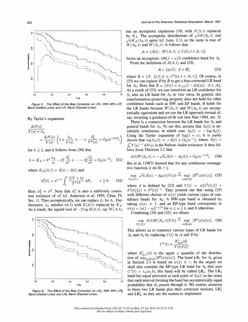
Figure 5. The Effect of the Bias Correction on LR1; With 95% LRcj Band (Dotted Lines) and LR1 Band (Dashed Lines).
By Taylor's expansion,
AN(s)
Y(s) + An
Y ) ( + Y() + + yk(S) +Op(r k/2))
for k > 1, and it follows from (30) that
2An &2 An ..+&2 An531 0= KA + -n i + +2 4 -5 +QOp(n-3), (31)
where KA(A, t) = A(t) - A(t) and
&r2( = nr+1 t I(Y > 0) dN r > 0. (32) r ~~~ yr+2
Here c = 2. Note that 6. is also a uniformly consis- tent estimator of a2 (cf. Andersen et al. 1993, Chap. IV, Sec. 1). Thus asymptotically, we can replace (r by &r. Fur- thermore, An satisfies (A. 1) with K(S, t) replaced by KA. As a result, the signed root of -2 log R(A, t), say W(A, t),
?. . ... ....-i ,. .
fi~ ~ ~ ~I ....'--
0 0 0.2 0.4 0.6 0.8 1.0
Time
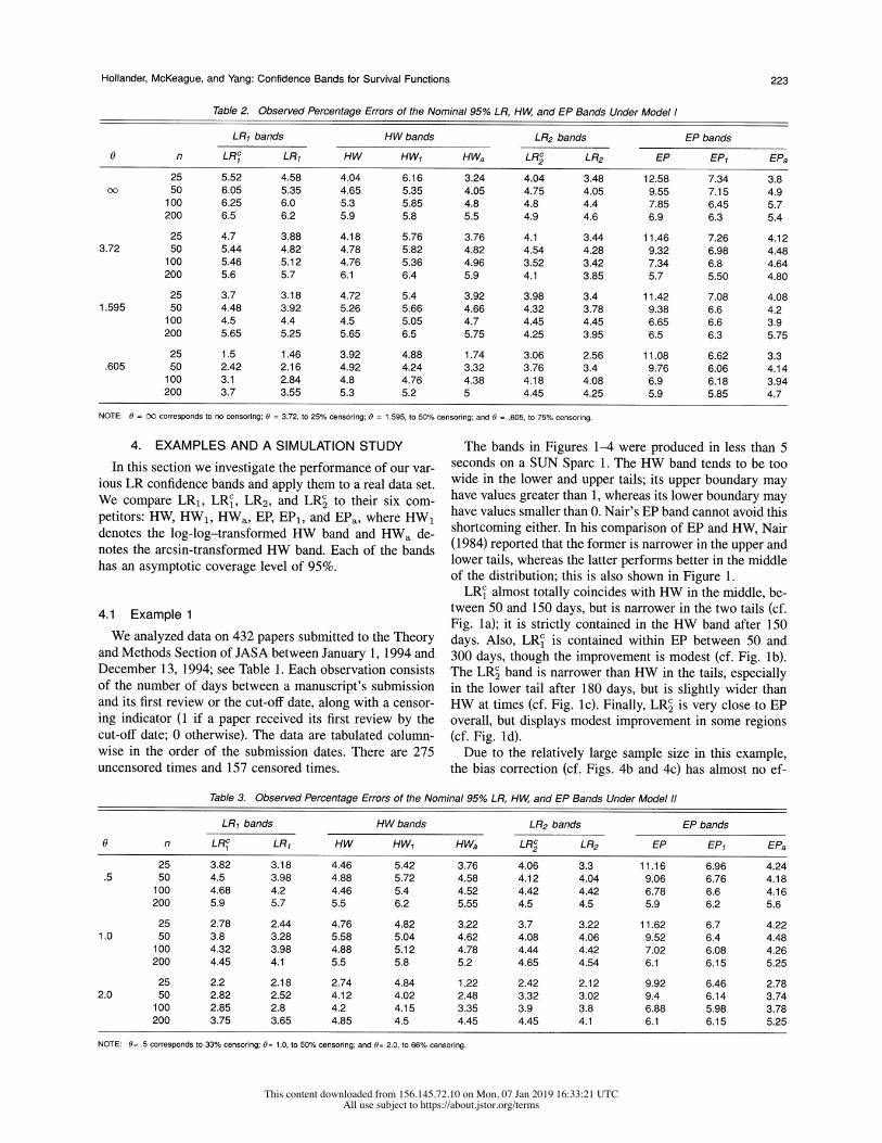
Figure 6. The Effect of the Bias Correction on LR2; With 95% LR2C Band (Dotted Lines) and LR2 Band (Dashed Lines).
has an asymptotic expansion (19), with K(S, t) replaced by KA. The asymptotic distributions of #K(So, t) and
V/_KA(AO, t) agree (cf. Lem. 2.1), so the same is true of W(Ao, t) and W(So, t). It follows that
A = {A(t): IW(A, t)I < C(t), t E [0, 7]}
forms an asymptotic 100(1 - a)% confidence band for Ao. From the definition of R(A, t) and (29),
A= {q)(S): S E 3} (33)
where B = {S: L2(S, t) < C2(t), t E [0,wT]}. Of course, in (33) we can replace B by B to get a bias-corrected LR band for Ao. Note that B = {S(t) = 7r,<t(1 - dA(s)): A E A}. As a result of (33), we can transform an LR confidence for SO into an LR band for Ao or vice versa. In general, this transformation-preserving property does not hold for other confidence bands such as HW and EP bands. It holds for the LR bands because W(So,t) and W(Ao,t) are asymp- totically equivalent and we use the LR approach instead of, say, inverting a goodness-of-fit test (see Nair 1984, sec. 3).
There is a connection between the LR bands for So and general bands for Ao. To see this, assume that So (t) is ab- solutely continuous, in which case AO (t) = - log So (t). Using the Taylor expansion of log(l + x), it is easily shown that logSn(t) = -A(t) + 0p(n-1), where A(t) =
fg Y (s)-1 dN(s) is the Nelson-Aalen estimator. It then fol- lows from Theorem 2.1 that
& (t)W(So It) = -v/-n-(A(t) - Ao(t)) + Op(n-1/2). (34)
Bie et al. (1987) showed that for any continuous nonnega-
tive function b on [0, r ],
sup v/A(x)-Ao(x)lV(x) D sup IB0(x)b(x)l, (35) O<x<r xE[O,d]
where d is defined by (22) and V(t) = 0f{82(t)/[j + 8r2(t)]}{1 + 8r2(t)}-1. They pointed out that using (35) with different choices of b(x) yields various types of con- fidence bands for Ao: A HW-type band is obtained by taking b(x) - 1, and an EP-type band corresponds to b(U) = [u(1 - U)]-1/2 for a < u < b, and 0 otherwise.
Combining (34) and (35), we obtain
sup 8c(t)W(S0,t)lV(t) i sup IB0(x)b(x)l. (36) O<t<r xE [O,d]
This allows us to construct various types of LR bands for
Ao and So by replacing C(t) in A and B by
C* () K'q, ,(d) C(t) V(t)8f(t)
where Kq,(d) is the upper aO quantile of the distribu- tion of SUPXE[O,d] IB0(x)b(x)l. The band LR1 for SO given in Section 2.1 is based on b(x) _ 1. In the sequel we shall also consider the EP-type LR band for So that uses C*(t) = eO(a,b); this band will be called LR2. The LR2 band has equal precision at each point of So(t) in the sense that each interval forming the band has asymptotically equal probability that S0 passes through it. We restrict attention to these two LR bands plus their corrected versions, LR~ and LRC2, as they are the easiest to implement.
This content downloaded from 156.145.72.10 on Mon, 07 Jan 2019 16:33:21 UTCAll use subject to https://about.jstor.org/terms
Hollander, McKeague, and Yang: Confidence Bands for Survival Functions 223
Table 2. Observed Percentage Errors of the Nominal 95% LR, HW, and EP Bands Under Model I
LR1 bands HW bands LR2 bands EP bands
0 n LRc LR1 HW HW1 HWa LR2c LR2 EP EP1 EPa
25 5.52 4.58 4.04 6.16 3.24 4.04 3.48 12.58 7.34 3.8 oo 50 6.05 5.35 4.65 5.35 4.05 4.75 4.05 9.55 7.15 4.9
100 6.25 6.0 5.3 5.85 4.8 4.8 4.4 7.85 6.45 5.7 200 6.5 6.2 5.9 5.8 5.5 4.9 4.6 6.9 6.3 5.4
25 4.7 3.88 4.18 5.76 3.76 4.1 3.44 11.46 7.26 4.12 3.72 50 5.44 4.82 4.78 5.82 4.82 4.54 4.28 9.32 6.98 4.48
100 5.46 5.12 4.76 5.36 4.96 3.52 3.42 7.34 6.8 4.64 200 5.6 5.7 6.1 6.4 5.9 4.1 3.85 5.7 5.50 4.80
25 3.7 3.18 4.72 5.4 3.92 3.98 3.4 11.42 7.08 4.08 1.595 50 4.48 3.92 5.26 5.66 4.66 4.32 3.78 9.38 6.6 4.2
100 4.5 4.4 4.5 5.05 4.7 4.45 4.45 6.65 6.6 3.9 200 5.65 5.25 5.65 6.5 5.75 4.25 3.95 6.5 6.3 5.75
25 1.5 1.46 3.92 4.88 1.74 3.06 2.56 11.08 6.62 3.3 .605 50 2.42 2.16 4.92 4.24 3.32 3.76 3.4 9.76 6.06 4.14
100 3.1 2.84 4.8 4.76 4.38 4.18 4.08 6.9 6.18 3.94 200 3.7 3.55 5.3 5.2 5 4.45 4.25 5.9 5.85 4.7
NOTE: 0 = oo corresponds to no censoring; 0 = 3.72, to 25% censoring; 0 = 1.595, to 50% censoring; and 0 = .605, to 75% censoring.
4. EXAMPLES AND A SIMULATION STUDY
In this section we investigate the performance of our var- ious LR confidence bands and apply them to a real data set. We compare LR1, LR', LR2, and LR' to their six com- petitors: HW, HW1, HWa, EP, EP1, and EPa, where HW1 denotes the log-log-transformed HW band and HWa de- notes the arcsin-transformed HW band. Each of the bands has an asymptotic coverage level of 95%.
4.1 Example 1
We analyzed data on 432 papers submitted to the Theory and Methods Section of JASA between January 1, 1994 and December 13, 1994; see Table 1. Each observation consists of the number of days between a manuscript's submission and its first review or the cut-off date, along with a censor- ing indicator (1 if a paper received its first review by the cut-off date; 0 otherwise). The data are tabulated column- wise in the order of the submission dates. There are 275 uncensored times and 157 censored times.
The bands in Figures 1-4 were produced in less than 5 seconds on a SUN Sparc 1. The HW band tends to be too wide in the lower and upper tails; its upper boundary may have values greater than 1, whereas its lower boundary may have values smaller than 0. Nair's EP band cannot avoid this shortcoming either. In his comparison of EP and HW, Nair (1984) reported that the former is narrower in the upper and lower tails, whereas the latter performs better in the middle of the distribution; this is also shown in Figure 1.
LR' almost totally coincides with HW in the middle, be- tween 50 and 150 days, but is narrower in the two tails (cf. Fig. la); it is strictly contained in the HW band after 150 days. Also, LR' is contained within EP between 50 and 300 days, though the improvement is modest (cf. Fig. lb). The LR' band is narrower than HW in the tails, especially in the lower tail after 180 days, but is slightly wider than HW at times (cf. Fig. ic). Finally, LR' is very close to EP overall, but displays modest improvement in some regions (cf. Fig. Id).
Due to the relatively large sample size in this example, the bias correction (cf. Figs. 4b and 4c) has almost no ef-
Table 3. Observed Percentage Errors of the Nominal 95% LR, HW, and EP Bands Under Model 11
LR1 bands HW bands LR2 bands EP bands
0 n LRc LR1 HW HW1 HWa LR2c LR2 EP EP1 EPa
25 3.82 3.18 4.46 5.42 3.76 4.06 3.3 11.16 6.96 4.24 .5 50 4.5 3.98 4.88 5.72 4.58 4.12 4.04 9.06 6.76 4.18
100 4.68 4.2 4.46 5.4 4.52 4.42 4.42 6.78 6.6 4.16 200 5.9 5.7 5.5 6.2 5.55 4.5 4.5 5.9 6.2 5.6
25 2.78 2.44 4.76 4.82 3.22 3.7 3.22 11.62 6.7 4.22 1.0 50 3.8 3.28 5.58 5.04 4.62 4.08 4.06 9.52 6.4 4.48
100 4.32 3.98 4.88 5.12 4.78 4.44 4.42 7.02 6.08 4.26 200 4.45 4.1 5.5 5.8 5.2 4.65 4.54 6.1 6.15 5.25
25 2.2 2.18 2.74 4.84 1.22 2.42 2.12 9.92 6.46 2.78 2.0 50 2.82 2.52 4.12 4.02 2.48 3.32 3.02 9.4 6.14 3.74
100 2.85 2.8 4.2 4.15 3.35 3.9 3.8 6.88 5.98 3.78 200 3.75 3.65 4.85 4.5 4.45 4.45 4.1 6.1 6.15 5.25
NOTE: 0= .5 corresponds to 33% censoring; 0= 1.0, to 50% censoring; and 0= 2.0, to 66% censoring.
This content downloaded from 156.145.72.10 on Mon, 07 Jan 2019 16:33:21 UTCAll use subject to https://about.jstor.org/terms
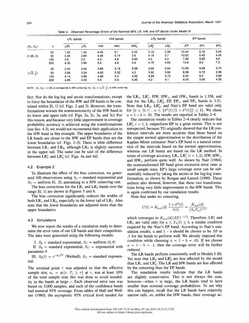
224 Journal of the American Statistical Association, March 1997
Table 4. Observed Percentage Errors of the Nominal 95% LR, HW, and EP Bands Under Model 1ll
LR1 bands HW bands LR2 bands EP bands
(01, 02) n LRC LR, HW HW2 HWa LR2 LR2 EP EP, EPa
25 1.92 1.46 4.46 5.1 2.42 3.16 2.38 10.44 6.18 3.26 (1.35, 2) 50 3.38 2.84 4.98 5.14 3.9 4.18 3.7 10.62 6.42 4.46
100 3.8 3.2 4.3 4.8 3.95 4.5 4.2 7.45 5.65 4.2 200 4.35 3.95 5.0 4.9 4.9 4.75 4.65 10.6 8.0 7.3
25 2.42 2.04 3.88 5.18 2.98 3.66 2.84 10.58 6.68 3.74 (V2,) 50 3.56 3.24 4.62 5.52 4.2 3.82 3.66 8.58 6.72 3.98
100 4.14 3.88 4.88 5.3 4.92 3.84 3.72 6.52 6.2 3.88 200 4.85 4.55 5.5 5.9 5.45 4.3 4.1 6.05 5.65 4.95
NOTE: (01, 02) = (1.35, 2) corresponds to 50% censoring; (0i, 02) = (62 2), to 35% censoring.
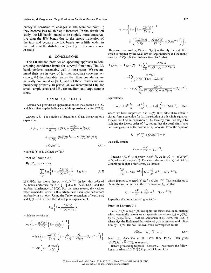
fect. Nor do the log-log and arcsin transformations, except to force the boundaries of the HW and EP bands to be con- tained within [0, 1] (cf. Figs. 2 and 3). However, the trans- formations worsen the nonmonotonicity of the HW band in its lower and upper tails (cf. Figs. 2a, 2c, 3a, and 3c). For this reason, and because very little improvement in coverage probability accuracy is achieved using the transformations (see Sec. 4.3), we would not recommend their application to the HW band in this example. The upper boundaries of the LR bands are closer to the HW and EP bands than are the lower boundaries (cf. Figs. 1-3). There is little difference between LR1 and LR2, although LR2 is slightly narrower in the upper tail. The same can be said of the difference between LR' and LR' (cf. Figs. 4a and 4d).
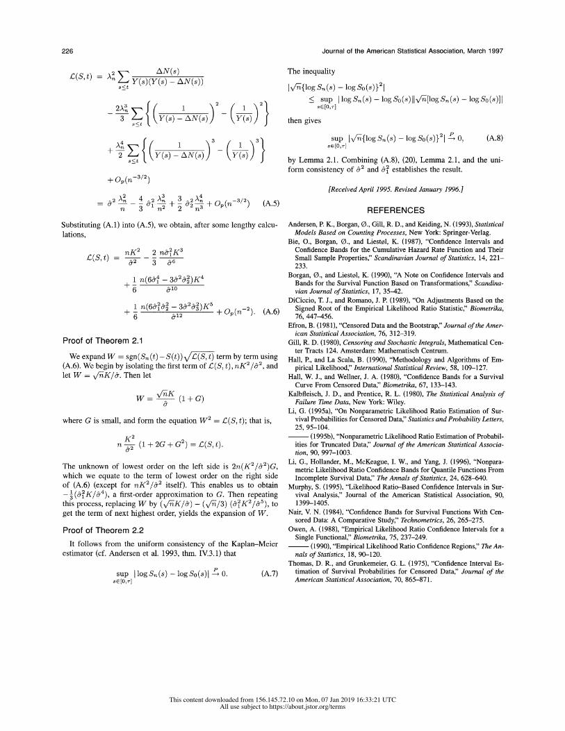
4.2 Example 2
To illustrate the effect of the bias correction, we gener- ated 100 observations using So = standard exponential and Sc = uniform (0, .5), amounting to a 50% censoring rate.
The bias corrections for the LR1 and LR2 bands over the range [0, 1] are shown in Figures 5 and 6.
The bias correction significantly reduces the widths of both LR1 and LR2, especially in the lower tail of LR1. Also note that the lower boundaries are adjusted more than the upper boundaries.
4.3 Simulations
We now report the results of a simulation study to deter- mine the error rates of our LR bands and their competitors. The data were generated using the following models:
I. So = standard exponential, Sc = uniform (0, 0) II. So = standard exponential, Sc = exponential with
parameter 0
III. SO(t) = e-6lt82 (Weibull), Sc = standard exponen- tial.
The terminal point T was adjusted so that the effective sample size, nr = #{i: Ti > T} at T, was at least 10% of the total sample size; this was done to avoid instabil- ity in the bands at large T. Each observed error rate was based on 5,000 samples, and each of the confidence bands had nominal 95% coverage. From tables of Hall and Well- ner (1980), the asymptotic 95% critical level needed for
the LR1, LRc, HW, HW1, and HWa bands is 1.358, and that for the LR2, LRc, EP, EP1, and EPa bands is 3.31. Note that LR2, LRc, and Nair's EP band are valid only
for {t E [0, T] : a < {1&2(t)/[l + &2(t)]} < b}. We chose a = 1 - b = .05. The results are reported in Tables 2-4.
The simulation results in Tables 2-4 clearly indicate that LRC, i = 1, 2, outperform EP to a great extent. This is not unexpected, because TG originally showed that the LR con- fidence intervals are more accurate than those based on the simple normal approximation to the distribution of the Kaplan-Meier estimator. Nair's EP band is a natural exten- sion of the intervals based on the normal approximation, whereas our LR bands are based on the LR method. In terms of coverage accuracy, LRi, LRc (i = 1, 2), HW, HW1, and HWa perform quite well. As shown by Nair (1984), the nontransformed EP band gives excessive error rates at small sample sizes. EP's large coverage error can be sub- stantially reduced by taking the arcsin or the log-log trans- formation, as shown by Borgan and Liest0l (1990). These authors also showed, however, that these two transforma- tions bring very little improvement to the HW bands. This is again confirmed by our simulation results.
Note that under no censoring,
C0(t) = Kq, a(d) 1 + 82 (t) _Kq, a(d) & ( t) ( n ) 1 /2
which converges to Kq,ae(d)(SF)-1/2 Therefore, LRc and LR1 are valid only for a < Fn (t) < b, a similar condition required by the Nair's EP band. According to Nair's sim- ulation results, a and 1 - b should be chosen to be .05 or .1 for the bands to perform well. We already imposed this condition while choosing a = 1 - b = .05. If we choose a = 1 - b = .1, then the coverage error will be further reduced.
The LR bands perform consistently well in Models I-III. Yet note that LR2 and LRc are less affected by the model than LR1 and LRc. The LR and HW bands are less affected by the censoring than the EP bands.
The simulation results indicate that the LR bands are slightly conservative. This is not always the case, however-when T is large, the LR bands tend to have smaller than nominal coverage probabilities. To see why this can happen, recall that the LR bands have relatively narrow tails, so, unlike the HW bands, their coverage ac-
This content downloaded from 156.145.72.10 on Mon, 07 Jan 2019 16:33:21 UTCAll use subject to https://about.jstor.org/terms
Hollander, McKeague, and Yang: Confidence Bands for Survival Functions 225
curacy is sensitive to changes in the terminal point T; they become less reliable as T increases. In the simulation study, the LR bands tended to be slightly more conserva- tive than the HW bands due to the strong truncation of the tails and because the LR bands are a little wider in the middle of the distribution. (See Fig. lc for an instance of this.)
5. CONCLUSIONS
The LR method provides an appealing approach to con-
structing confidence bands for survival functions. The LR
bands perform reasonably well in most cases. We recom- mend their use in view of (a) their adequate coverage ac- curacy, (b) the desirable feature that their boundaries are naturally contained in [0, 1], and (c) their transformation- preserving property. In particular, we recommend LR' for small sample sizes and LR2 for medium and large sample sizes.
APPENDIX A: PROOFS
Lemma A. 1 provides an approximation for the solution of (1 5),
which is a first step in finding a suitable approximation for L(S, t).
Lemma A.]. The solution of Equation (15) has the asymptotic
expansion
An(S,t) = - K(S,t) + nIM(t) K 2(S, t)
n {3&2-(t)&-2(t) t)}K(S,t) 810 (t)
+ Op(n-1) (A.1)
where K(S, t) is defined by (18).
Proof of Lemma A.1
By (15), An satisfies
Elog I1- yN(s)() }=log S(t). (A.2)
Li (1995a) has shown that An = Op(nr1/2). In fact, this order of An holds uniformly for t E [0, T] due to (A.7), (A.8), and the uniform consistency of &2 (t). For the same reason, the various other remainder terms in this article have their specified orders
uniformly in t E [0, T]. Using the Taylor expansions of log(l + x)
and 1/(1 + x), we can then develop an expansion of
log I1- AN(s) g Y(s) +An f
which we rewrite as
lo A1_/N(s) (1+An) }
= log{1~ _ Fjj) (1k;() + Y2(s) -Op(n-3/2) }
l log (1 - ____ )
+ log{I+ (I - ) > )
AB,AN(s)_ A 2AN(s)52 ( An/ V( 2 \N ( + Op(n-5/ Y2 (S) Y3 (S)2j
Here we have used n/Y(s) = Op(1) uniformly for s E [0, T], which is implied by the weak law of large numbers and the mono- tonicity of Y(s). It then follows from (A.2) that
logS(t) = log Sn(t) + An (S)(Y(S)-N(s)) S<t
_2 AN(s) y2(S)(Y(s) - AN(s)) s<t
+*** + A,n S Y5(S)(Y(S) - AN(s)) + S<t
Equivalently,
^2 An_ J2 An+ J2 An +O(n ), (3 O=K+u --al-n + + 174 + Op(n- (A.3) n n2 n5
where we have suppressed t in T(t). It is difficult to obtain a closed-form expression for An, the solution of this whole equation. Instead, we find an expansion of An term by term. We begin by isolating the lowest order of An, noting that the coefficients have decreasing orders as the powers of An increase. From the equation
K+&2 A+On (n 1)=0,
we easily obtain
n=- ^2 +P
Because nK/&2 is of order Op(nl/2), we let A' =-n(K/&2) + G, where G is op(n 1/2). Then we substitute this A' into (A.3). Combining higher-order terms, we obtain
[ ^2 1 ^2 + Op(- ,3/2I G= IK2-pn /)
which implies G = (ni&2/&6)K2 + Op(n-r1/2). This enables us to obtain the second term in the expansion of An, so that
_nK n K2 + O(-1/2)
82 6
Repeating this iteration will give (A.1).
Proof of Lemma 2.1
Let 4(S) (t) = log S(t). We apply the functional delta method, which essentially allows us to approximate Vn(p(Sn) - (P(So)) by dso(So)(Vni(Sn - So)) (cf. Andersen et al. 1993, thm. 11.8.1), where dp, the Hadamard derivative of p, is pointwise multiplica- tion by -1/S. The well-known weak convergence result
n (Sn - SO) DSOU (A.4)
(see, e.g., Andersen et al. 1993, thin. IV.3.2) then gives
<~K(S0,t) -*U(t), as required.
Before proceeding to prove Theorem 2.1, we record the follow-
ing expansion of L:(S, t) (cf. proof of Lem. Al1):
This content downloaded from 156.145.72.10 on Mon, 07 Jan 2019 16:33:21 UTCAll use subject to https://about.jstor.org/terms
226 Journal of the American Statistical Association, March 1997
L (S, t) =AnZ ~ Y~?~ s<t (s) (Y(s)-(s))
n24 E{(y(sv1AN(s)) (Yv))}
+ 2 s{(y(s)-AN(s))3 (;S)) }
+ Op(n-3/2)
2 An 4 2 An 3 J2A 3/2 n7 - - 7 + - .2 -n + oP(nJ12 (A.5)
Substituting (A. 1) into (A.5), we obtain, after some lengthy calcu- lations,
t nK2 2 n&2 K3 L:(S,t) = &2 3 &6
1 n(6&4 -3&2&2 )K4
6 &10o
1 n(6&2&2 - 3&2&2 )K5 + O5(n72) (A.6) +6 &12
Proof of Theorem 2.1
We expand W = sgn(Sn (t) - S(t)) /(S, t) term by term using (A.6). We begin by isolating the first term of L(S, t), nK2/&2, and
let W = VYK/l&. Then let
W n- jK(10 w = (1+ G)
where G is small, and form the equation W2 = L(S, t); that is,
K2 (I + 2G + G2) = L:(St
The unknown of lowest order on the left side is 2n(K2/&2)G, which we equate to the term of lowest order on the right side of (A.6) (except for nK2/8-2 itself). This enables us to obtain - (&f2K/&f4), a first-order approximation to G. Then repeating this process, replacing W by (V'YK/l&) - (xY/13) (&f2K2/&5), to get the term of next highest order, yields the expansion of W.
Proof of Theorem 2.2
It follows from the uniform consistency of the Kaplan-Meier estimator (cf. Andersen et al. 1993, thm. IV.3.1) that
sup logSn(s)-logSo(s) l O. (A.7) s E [O,rT]
The inequality
|ifi{log Sn(s) - log So(s)} 21
< sup |logSn (s) -logSo(s)j|V| [logSn(S) -logSo(s)]I s E [0o,]
then gives
sup IV{logSn(s) s)}21 0, (A.8) sE [o,TJ
by Lemma 2.1. Combining (A.8), (20), Lemma 2.1, and the uni- form consistency of &2 and 8-2 establishes the result.
[Received April 1995. Revised January 1996.]
REFERENCES
Andersen, P. K., Borgan, 0., Gill, R. D., and Keiding, N. (1993), Statistical Models Based on Counting Processes, New York: Springer-Verlag.
Bie, O., Borgan, 0., and Liest0l, K. (1987), "Confidence Intervals and Confidence Bands for the Cumulative Hazard Rate Function and Their
Small Sample Properties," Scandinavian Journal of Statistics, 14, 221- 233.
Borgan, 0., and Liest0l, K. (1990), "A Note on Confidence Intervals and Bands for the Survival Function Based on Transformations," Scandina- vian Journal of Statistics, 17, 35-42.
DiCiccio, T. J., and Romano, J. P. (1989), "On Adjustments Based on the Signed Root of the Empirical Likelihood Ratio Statistic," Biometrika, 76, 447-456.
Efron, B. (1981), "Censored Data and the Bootstrap," Journal of the Amer- ican Statistical Association, 76, 312-319.
Gill, R. D. (1980), Censoring and Stochastic Integrals, Mathematical Cen- ter Tracts 124. Amsterdam: Mathematisch Centrum.
Hall, P., and La Scala, B. (1990), "Methodology and Algorithms of Em- pirical Likelihood," International Statistical Review, 58, 109-127.
Hall, W. J., and Wellner, J. A. (1980), "Confidence Bands for a Survival
Curve From Censored Data," Biometrika, 67, 133-143. Kalbfleisch, J. D., and Prentice, R. L. (1980), The Statistical Analysis of
Failure Time Data, New York: Wiley.
Li, G. (1995a), "On Nonparametric Likelihood Ratio Estimation of Sur- vival Probabilities for Censored Data," Statistics and Probability Letters, 25, 95-104.
(1995b), "Nonparametric Likelihood Ratio Estimation of Probabil- ities for Truncated Data," Journal of the American Statistical Associa- tion, 90, 997-1003.
Li, G., Hollander, M., McKeague, I. W., and Yang, J. (1996), "Nonpara- metric Likelihood Ratio Confidence Bands for Quantile Functions From
Incomplete Survival Data," The Annals of Statistics, 24, 628-640. Murphy, S. (1995), "Likelihood Ratio-Based Confidence Intervals in Sur-
vival Analysis," Journal of the American Statistical Association, 90, 1399-1405.
Nair, V. N. (1984), "Confidence Bands for Survival Functions With Cen- sored Data: A Comparative Study," Technometrics, 26, 265-275.
Owen, A. (1988), "Empirical Likelihood Ratio Confidence Intervals for a Single Functional," Biometrika, 75, 237-249.
(1990), "Empirical Likelihood Ratio Confidence Regions," The An- nals of Statistics, 18, 90-120.
Thomas, D. R., and Grunkemeier, G. L. (1975), "Confidence Interval Es- timation of Survival Probabilities for Censored Data," Journal of the American Statistical Association, 70, 865-871.
This content downloaded from 156.145.72.10 on Mon, 07 Jan 2019 16:33:21 UTCAll use subject to https://about.jstor.org/terms
Related Documents


![Asymptotic Confidence Bands for Copulas Based on …file.scirp.org/pdf/AM_2015112516141818.pdf · estimator of Deheuvels [7]. Omelka, Gijbels and Veraverbeke [10]proposed improved](https://static.cupdf.com/doc/110x72/5b81ddba7f8b9ae97b8d37b7/asymptotic-confidence-bands-for-copulas-based-on-filescirporgpdfam-estimator.jpg)

