Life Cycle Costing: an effective asset management tool “Applying LCC contributes to more cost-effective management control of the production facilities of small and medium enterprises (SMEs)” Master of Science in Asset Management Control International Masters School Student: Bas Kemps Supervisor: Ir. Peter van Gestel Date: 12-6-2012

Welcome message from author
This document is posted to help you gain knowledge. Please leave a comment to let me know what you think about it! Share it to your friends and learn new things together.
Transcript

�
Life Cycle Costing:
an effective
asset management tool
“Applying LCC contributes to more cost-effective
management control of the production
facilities of small and medium enterprises (SMEs)”
Master of Science in
Asset Management Control
International Masters School
Student: Bas Kemps
Supervisor: Ir. Peter van Gestel
Date: 12-6-2012

ACKNOWLEDGEMENTS
I would like to dedicate this dissertation to my wife and colleagues. Writing this master’s thesis has
been very time-consuming. This has certainly had various consequences at home as well as at work.
Thanks to the understanding of these people, it has nonetheless been possible to complete this
thesis.
For controlling the quality of this dissertation, I would also like to thank Niek van Nunen and Peter
van Gestel. To complete this phase, Niek van Nunen was designated company supervisor. Peter van
Gestel has been so good as to act as supervisor on behalf of the master’s program.

Dissertation document B. Kemps Page 3
Summary
This master’s thesis seeks to develop and accept the following hypothesis: applying LCC analysis
results in more cost-effective management control of production facilities of SMEs. Research on the
sub questions has demonstrated that there is a difference in Life Cycle Costing and Life Cycle Cost
Analysis. Life cycle costing takes into account all costs of an asset throughout its intended lifespan,
resulting in a total cost of ownership calculation. Life Cycle Cost Analysis can be described as a cost-
comparing method of possible alternatives, using the Life Cycle Costing approach. Because LCC
analysis compares alternatives, only the differences between the alternatives translated into costs
will have to be compared.
In relation to the purchasing process of assets, Veteka, the pilot company, can be seen as the user of
the installations. A customer perspective is therefore the most suitable one. In order to provide
evidence relevant to the hypothesis, four case studies are described. The purpose is to compare
alternatives for each case by means of an LCC analysis method. Because in each case the purpose is
to compare different alternatives, it is not necessary to implement a complete life cycle costing
model that would result in a total cost of ownership of the different alternatives. For the purposes of
this thesis, it is sufficient to implement an LLC analysis in which only the cost differences between
two or more alternatives are taken into account. Costs that are the same for two alternatives can be
eliminated from consideration.
One of the sub questions was to introduce a suitable model in order to make an objective
comparison. Dell'Isola and Kirk [2003] describe a model which meets the needs regarding this thesis.
The model has been developed in Excel and is therefore also very easy to use. It incorporates a
discount and escalation rate and calculates the present worth difference between two or more
alternatives. Although Dell’Isola and Kirk’s book [2003] describes the sensitivity and uncertainty in
input parameters, it is barely possible to implement their method in one simple model. As a result of
experience with the @Risk program, Dell'Isola & Kirk’s model has been adapted in order to
implement the @Risk program. The adapted model makes it possible to calculate discount rate,
escalation rate, sensitivity, and uncertainty, resulting in the present worth difference of two
alternatives at the same time. With the @Risk program it is possible to generate graphs to visualize
both the impact of the different input parameters and the likelihood of an outcome to be positive or
negative.
The results of the different cases dealt with provide sufficient evidence for the hypothesis to be
accepted. Conducting an LCC analysis creates transparancy among the different cost drivers. Through
LCC analysis, the management can gather a lot of information on the financial concequences of
different alternatives, and with relatively little effort. For instance, an LCC analysis will reflect the
impact of hidden costs. Creating transparancy about the different relevant costs results in the fact
that more balanced choices can and will be made. To refine the uncertainty and sensitivity in the
different costs it is strongly recommended that further investigation is carried out into reliability,
availability and maintainability.
Although this type of analysis helps the purchasing process of installations, it does not indicate the
total expected revenues over the intended life span. For this, an analysis which takes into account all
costs and profits should be conducted. The result is a net present value difference.

Dissertation document B. Kemps Page 4
Currently, at Veteka, the pilot company, the data needed to conduct this type of analysis are
insufficient. When further investigation is carried out into discount and escalation rates, and
maintainability, availability and reliability, this broader type of analysis will be useful for making
proper cost calculations.

Dissertation document B. Kemps Page 5
Index
Acknowledgements ................................................................................................................................. 2
Summary ................................................................................................................................................. 3
Index ........................................................................................................................................................ 5
1 Introduction ................................................................................................................................... 10
1.1 Life cycle costing and total cost of ownership ...................................................................... 10
1.2 Statement of the research problem ...................................................................................... 11
1.3 Research questions................................................................................................................ 12
1.4 Research method .................................................................................................................. 14
1.5 Relation between research questions and model ................................................................. 15
1.6 Definitions and Terms ........................................................................................................... 16
2 Scope of a Life Cycle and Life Cycle Costing .................................................................................. 18
2.1 General ....................................................................................................................................... 18
2.2 Life cycle ................................................................................................................................ 18
2.2.1 The life cycle of the market .................................................................................................. 18
2.2.2 The life cycle of the development/production process ....................................................... 19
2.3 Life cycle cost tree ................................................................................................................. 22
2.4 Difference between Life cycle costing and Life Cycle cost analysis ...................................... 23
2.5 Area of interest in LCC analysis ............................................................................................. 24
3 Models ........................................................................................................................................... 26
3.1 Introduction .......................................................................................................................... 26
3.2 Commonly used models ........................................................................................................ 26
3.3 Models relevant to this study ................................................................................................ 29
3.4 Cost breakdown structure ..................................................................................................... 29
3.5 Discount and Escalation rate ................................................................................................. 30
3.6 Uncertainty and sensitivity ................................................................................................... 31
4 The purchasing process ................................................................................................................. 32

Dissertation document B. Kemps Page 6
4.1 Introduction ................................................................................................................................ 32
4.2 Purchasing policy of SMEs ..................................................................................................... 32
4.3 Reliability, availability and maintainability of current installations ...................................... 33
4.4 Improvements expected from implementing LCC analysis .................................................. 35
5 Cases .............................................................................................................................................. 36
5.1 Description of the cases .............................................................................................................. 36
5.1.1 Weinig versus Leadermac .............................................................................................. 36
5.1.2 Moulding Cutter Head ................................................................................................... 36
5.1.3 Coating line .................................................................................................................... 37
5.1.4 Double vacuum box ....................................................................................................... 39
5.2 Input parameters ......................................................................................................................... 40
5.2.1 Starting points ............................................................................................................... 40
5.2.2 Manufacture parameters .............................................................................................. 40
5.3 Results ........................................................................................................................................ 41
5.3.1 Weinig versus Leadermac .............................................................................................. 42
5.3.2 Moulding Cutter Head ................................................................................................... 42
5.3.3 Coating line .................................................................................................................... 43
5.3.4 Double vacuum box ....................................................................................................... 43
5.4 Conclusions to separate cases ..................................................................................................... 44
6 Efforts involved in Life Cycle Costing ................................................................................................. 45
6.1 Human efforts ....................................................................................................................... 45
6.2 Cost of LCC analysis ............................................................................................................... 45
7 Conclusions ....................................................................................................................................... 47
8 Recommendations ............................................................................................................................. 50
9 Reflection on the impact of LCC on company and management ...................................................... 51
Literature ............................................................................................................................................... 52
Appendix ................................................................................................................................................ 54

Dissertation document B. Kemps Page 7
Appendix 1: Dell’Isola’s Model .......................................................................................................... 54
Appendix 2: Present worth (of annuity) factor ................................................................................. 55
Appendix 3: Effect of the discount rate ............................................................................................ 56
Appendix 4: Input parameters and calculation sheets...................................................................... 57
Appendix 4.1: input parameters Weinig versus Leadermac ......................................................... 57
Appendix 4.2: Calculation Weinig versus Leadermac ................................................................... 58
Appendix 4.4: calculation sheet Moulding cutter head ................................................................ 60
Appendix 4.5: Input parameters Coating line ............................................................................... 61
Appendix 4.6: Calculation sheet Coating line ................................................................................ 62
Appendix 4.7: Input parameters Double vacuum box .................................................................. 63
Appendix 4.8: Calculation sheet Double vacuum box ................................................................... 64
Appendix 5.1: Weinig versus Leadermac ...................................................................................... 66
Appendix 5.2: Moulding cutter head ............................................................................................ 69
Appendix 5.3: Coating line............................................................................................................. 72
Appendix 5.4: Double vacuum box ................................................................................................ 75
Appendix 6: Veteka, the pilot study .................................................................................................. 78

Dissertation document B. Kemps Page 8
Figure 1: Life cycle cost, consisting of acquisition costs and operations and maintenance 10
Figure 2: Exploratory-empirical research approach 14
Figure 3: different stages of a production life cycle 19
Figure 4: V-model 19
Figure 5: Life cycle assessment, design for environment approach 20
Figure 6: overall view of a life cycle 20
Figure 7: Area of interest in the life cycle from a customer point of view 21
Figure 8: Life cycle cost tree 22
Figure 9: Life cycle cost tree refined 23
Figure 10: Area of interest in LCC analysis for the pilot case 25
Figure 11: Life Cycle management domain 26
Figure 12: LCM, simplified for the purposes of this master thesis 27
Figure 13: Three layers of activity-based life cycle costing 28
Figure 14: Power lock system versus traditional moulding cutter head 37
Figure 15: Layout new coating line 38
Figure 16: Sophisticated transport system 39
Figure 17: Manufacture parameters 41
Figure 18: LCC analysis model 54
Table 1: Effect of the discount rate over the next 25 years 56
Table 2: Significant input parameters related to graph 1 66
Table 3: Significant input parameters related to graph 5 69
Table 4: Significant input parameters related to graph 9 72
Table 5: Significant parameters related to graph 13 75
Table 6: Essential characteristics of the replacement value of some used equipment 78

Dissertation document B. Kemps Page 9
Graph 1: Simple sensitivity analysis over the years, case 1 66
Graph 2: Distribution case 1 67
Graph 3: Uncertainty correlation case 1 67
Graph 4: sensitivity correlation case 1 68
Graph 5: Simple sensitivity analysis over the years, case 2 69
Graph 6: Distribution case 2 70
Graph 7: Uncertainty correlation case 2 70
Graph 8: Sensitivity correlation case 2 71
Graph 9: Simple sensitivity analysis over the years, case 3 72
Graph 10: Distribution case 3 73
Graph 11: Uncertainty correlation case 3 73
Graph 12: sensitivity correlation case 3 74
Graph 13: Simple sensitivity analysis over the years, case 4 75
Graph 14: Distribution case 4 76
Graph 15: Uncertainty analysis case 4 76
Graph 16: sensitivity correlation case 4 77
Dissertation document B. Kemps Page 10
1 Introduction
1.1 Life cycle costing and total cost of ownership
Life cycle costing is an economic management tool designed to evaluate economic consequences of
an item, system or facility over its lifespan, expressed in terms of equivalent cost, using baselines
identical to those used for initial cost. Life cycle costing is used to compare various options by
identifying and assessing economic impacts over the life of each option. [Dell'Isola & Kirk, 2003]
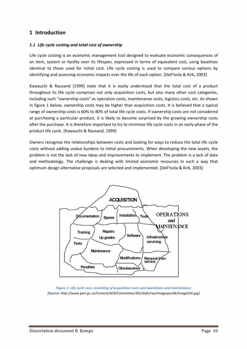
Kawauchi & Rausand [1999] state that it is easily understood that the total cost of a product
throughout its life cycle comprises not only acquisition costs, but also many other cost categories,
including such “ownership costs” as operation costs, maintenance costs, logistics costs, etc. As shown
in figure 1 below, ownership costs may be higher than acquisition costs. It is believed that a typical
range of ownership costs is 60% to 80% of total life cycle costs. If ownership costs are not considered
at purchasing a particular product, it is likely to become surprised by the growing ownership costs
after the purchase. It is therefore important to try to minimize life cycle costs in an early phase of the
product life cycle. [Kawauchi & Rausand, 1999]
Owners recognize the relationships between costs and looking for ways to reduce the total life cycle
costs without adding undue burdens to initial procurements. When developing the new assets, the
problem is not the lack of new ideas and improvements to implement. The problem is a lack of data
and methodology. The challenge is dealing with limited economic resources in such a way that
optimum design alternative proposals are selected and implemented. [Dell'Isola & Kirk, 2003]
Figure 1: Life cycle cost, consisting of acquisition costs and operations and maintenance
[Source: http://www.parl.gc.ca/Content/SEN/Committee/391/defe/rep/imagesjun06/image016.jpg]

Dissertation document B. Kemps Page 11
1.2 Statement of the research problem
Life cycle costing was originally designed for procurement purposes in the U.S. Department of
Defence [White & Ostwald, 1976] and is still most commonly used in the military sector and the
construction industry [Woodward, 1997]. Adoption of life cycle thinking has been very slow in other
industries [Lindholm & Suomala, 2005]. In a Finnish study, for instance, only 5% of large industrial
companies had used life cycle costing [Hyvönen, 2003]. These studies do not even mention the use of
life cycle costing in small and medium enterprises (SMEs).
Not much information is available regarding the use of life cycle costing within SMEs. Most decisions
are mainly based on experience, feelings and small basic calculations. For this reason there is only
little insight into the total cost of individual installations over their technical lifespan in SMEs.
To remain competitive and to maintain market position, SMEs have to continuously improve their
efficiency. As Emblemsvåg [2003] explains, the invention of the digital computer has created an
explosion in product variety at affordable prices because new manufacturing technologies enabled
mass production at an unprecedented scale. This development has resulted in a faster changing
environment in which techniques continuously change. As a result, companies have to secure the
purchasing policy of assets/installations in order to remain competitive. This study will concentrate
on the contribution of Life cycle cost analysis (LCC analysis) to the process of purchasing a new
production device in SMEs.
A small investigation among clients and suppliers has pointed out that SMEs rarely have a clear
insight into the total costs of individual installations over their technical lifespan. In order to make
cost-effective, well-founded decisions about new assets, it is essential to create transparency of all
costs over an asset’s technical lifespan (within a particular company). Life cycle cost calculations
could be a tool to gain insight in the total cost of ownership for different installations. Such
researchers as J. Emblemsvåg, B.S. Dhillon and H. Barringer have proved that life cycle cost
calculations contribute to a cost-effective management of assets. In the literature available, several
examples of life cycle costing models are provided. Although these examples are often about
complex “static” assets such as marine ships, (large) infrastructural projects, wind mill parks, power
plants, etc., there are also some examples which are similar in scale to assets in SMEs. [Barringer,
2003; Emblemsvåg, 2003; Korpi & Ala-Risku, post-2005; Dhillon, 2010] For instance, Barringer states
that life cycle cost calculations could be useful for investments starting between 10.000-25.000 US
dollars (in 2003). This statement will be discussed later in this thesis.
As mentioned before, the purchase policy of SMEs is often based on experience and general
knowledge. The question arises whether or not life cycle costing can help these companies to create
a more evidence-based purchase method. This is what this master’s thesis will be focused on. For this
particular case, the following hypothesis is developed:
“Applying LCC contributes to more cost-effective management control of production facilities of
SMEs.”
To test the hypothesis, the company Houtindustrie Veteka will serve as a pilot case. This company
was founded about 40 years ago. During these 40 years it has become one of the leading companies

Dissertation document B. Kemps Page 12
in supplying the Dutch construction market of houses with finished wooden mouldings. The company
is equipped with different production processes in order to profile and coat the wooden slats.
Within this company four individual cases will be discussed in order to find evidence to accept the
hypothesis.
1.3 Research questions
To provide a solution to the case described and to find evidence to prove the hypothesis, the
following research question is formulated:
“How can within a purchasing strategy life cycle cost analysis contribute to improve cost-effective
management control throughout SME’s?”
To find an answer to this question, different areas of interest have to be investigated and examined.
In order to perform a structured investigation seven sub questions are performed. Each sub question
contributes to the investigation on the different areas of interest to perform an answer on the
research question.
To provide an answer on the research question, first the research area has to be defined. For
example it is important to have insight in which cost parameters are of interest in the purchase
process of production installations and which are of minor importance? In this way the next sub
question is formulated:
1. What is the scope of life cycle cost analysis related to this case?
This question will be handled in chapter 2
Knowing the field of interest, first a literature study is done to create insight in the way LCC analysis
are conducted. It is believed that not all LCC calculations are performed in exactly the same way.
Investigation has to be carried out on which LCC model is suitable for this case and will it be possible
to extract a useful model for this study. This has led to perform the next sub questions:
2. Which commonly used models are available in the literature?
3. Which of the previously mentioned model(s) is/are suitable, and in what way is optimization
of one of these models (or a combination of models) possible, in order to develop a useful
model for production facilities within SMEs? These two questions will be handled in chapter
3

Dissertation document B. Kemps Page 13
In order to improve the purchasing strategy, it is important to have insight in the current purchasing
policy and all other relevant information available. With the knowledge gained from the previous
questions, necessary data to perform an LCC analysis can be derived. So besides the current
purchasing policy also data collection to fulfill the input parameters is needed. This has led to form
the next question:
4. How does the current purchasing process of installations take place, and what historical data
needed is at hand?
This question will be handled in chapter 4
Based on the previous questions some knowledge about LCC analysis and its boundaries is gained. In
order to stay focused on providing evidence to accept the hypothesis it becomes useful at this stage
to point out expected improvements. Therefore the next question is performed.
5. Which parts of the current purchasing process are expected to be improved with the
introduction of LCC?
This question will be handled in chapter 4
To provide evidence in order to accept the hypothesis four practical case studies within the pilot
company will be performed. These four cases are described in (section xx and xx). In these chapters
an experimental LCC analysis on each case is carried out, and the results will be presented. To
evaluate these outcomes the next sub questions are conducted.
6. What are the findings with the previously mentioned question when conducting an
experimental LCC analysis?
This question will be handled in chapter 5 (results and conclusions)
7. How are the efforts involved in conducting an LCC analysis related to the benefits of the LCC
analysis?
This question will be handled in chapter 6
With the total knowledge and insight gained on LCC analysis, and the answer on the last sub
questions it will be possible to derive conclusions on the stated hypothesis.
“Applying LCC contributes to more cost-effective management control of production facilities of
SMEs.”

Dissertation document B. Kemps Page 14
1.4 Research method
To guide this master’s thesis, the Exploratory-empirical research approach will be used. On initiation
of the project, a theoretical and practical investigation can be set up. This part of the research gains
insight in the available information and helps to clearly specify the problem definition. From this
theoretical basis and problem definition it is possible to design and expand an experimental model.
The empirical side of the research is mainly focused on deriving conclusions based on the
information of the experimental design and the theoretical and practical foundation. Purely empirical
research draws conclusions from results without any theoretical foundation. The figure below gives
an impression of the approach used. [Saunder, 2000]
Figure 2: Exploratory-empirical research approach
[Source: Saunder, 2000]
In this thesis, the hypothesis formulated forms the statement and foundation of the research. To
investigate the foundation, the problem definition will be defined by stating a central question and
sub questions. During the experimental system design, information will be gathered and structured.
The basis of a model will be designed. After this phase, the experimental model will be completed;
the practical results can be evaluated against the theoretical foundation and hypothesis.
Chapter 2,3 and 4 are mainly forming the exploratory research part of this thesis. In the fifth Chapter
four practical cases will be handled, this forms the empirical part of the research method. In chapter
5 and 7 the empirical research results will be discussed.

Dissertation document B. Kemps Page 15
1.5 Relation between research questions and model
To further define the relation of the investigation with the model used, the sub questions will be
assigned to a certain place in the model. Behind each block of the model, the appropriate sub
question(s) will be given.
Initiation
Theoretical &
practical foundation
Problem definition
Empirical
research results
Experimental
system design
In this specific part of the research the purpose of the research is pointed
out. This purpose can be clarified by the stated hypothesis which has to be
proven. In this part also general
A literature study will be performed to find out what theory is at hand
regarding this subject. With this knowledge an abstraction will be made to
distillate the scope and useful models of LCC related to this case (sub
question 2 & 1).
From the moment the scope and models are defined, the current purchase
process and available data needed has to be investigated. Expected
improvements also have to be pointed out.
(sub questions 1,4 & 5)
With the findings of the literature study and the problem definition a model
will be chosen and adjusted to make it suitable for this case. Four
experimental case studies will be performed by using this model (sub
question 3 & 6).
The results will be presented and a discussion will be started whether the
results correspond to the expectation. Moreover there will be discussed if
the efforts involved in conducting a LCC analysis will offset to the benefits
(sub question 6 & 7). A feedback to the theoretical & practical foundation
and the problem definition will be made.
The initiation of this research is caused by the development of new
constructors, the evolution of our own market and the need to gain more
precise insight into present and future costs of our installations

Dissertation document B. Kemps Page 16
1.6 Definitions and Terms
For reasons of clarity, some specific terms which will be used throughout this study will first be
explained.
Asset management: a management approach to manage all processes (specify, design,
produce, maintain and dispose) needed to achieve a capital asset capable to meet the
operational need in the most effective way for the customer/user. [Stavenuiter, 2002]
Asset Management Control: a management approach to manage and control, over the life
cycle, all processes (specify, design, produce, maintain and dispose) needed to achieve a
capital asset capable to meet the operational need in the most effective way for the
customer/user. [Stavenuiter, 2002]
Life cycle generaly: Life cycle definitions basically follow the same steps; these different steps
are:
o Development
o Introduction
o Growth
o Maturity
o Decline
When defining the life cycle of assets, the steps are different. The development/production
process approaches the life cycle from the conceptual stage till the phase of use,
maintenance and phase out. In section 2.2.2 this will be handled more detailed.
Life cycle cost: Emblemsvåg describes Life cycle costs as “the total costs that are incurred, or
may be incurred, in all stages of the product life cycle”. [Emblemsvåg, 2003]
Life cycle costing: Life cycle costing is an economic assessment of an item, area, system, or
facility that considers all significant costs of ownership over its lifespan, expressed in terms of
equivalent dollars. LCC is a technique that satisfies the requirements of owners for adequate
analyses of total costs. [Dell'Isola & Kirk, 2003] In extension, this technique/method can be
used to determine the total cost of ownership of an item.
Life cycle cost analysis: Life cycle cost analysis is an economic assessment of an item, system
or facility over its lifespan, expressed in terms of equivalent cost, using baselines identical to
those used for initial cost. Life cycle cost analysis is used to compare various options by
identifying and assessing economic impacts over the life of each option. [Dell'Isola & Kirk,
2003]
Life Cycle Analysis (LCA): LCA is an analytical tool of increasing importance for supply chain
management. It aims to provide the basis for decisions which will promote sustainable
development of our economies. Its strength is primarily related to the development of
cleaner production and products, in order to reduce material and energy use and emissions
harmful to the environment. [Stavenuiter, 2002]
Dissertation document B. Kemps Page 17
Life Cycle assessment: J. Stavenuiter [2002] explains in his book that life cycle assessment is
the same as life cycle analysis.
Discount Rate: a multiplicative number (calculated from a discount formula for a given
discount rate and interest period) that is used to convert costs and benefits occurring at
different times to a common time. Often, interest rate will be used as a synonym for discount
rate. Discount rate means the minimum attractive rate of return on an investment. [Dell'Isola
& Kirk, 2003]
Escalation rate: this rate has to be taken into account when price modifications of individual
items over time are greater than or less than the general discount/inflation rate.
Present worth (method): an economic method that requires conversion of costs and benefits
by discounting future cash flows to a baseline date. [Dell'Isola & Kirk, 2003]
The present worth can be defined for costs and benefits. When all discounted costs are
subtracted from all discounted benefits, one can determine the net present value.
Net present value: the standard criterion for deciding whether a program can be justified on
economic grounds is net present value. Net present value is computed by assigning monetary
values to benefits and costs, discounting future benefits and costs, using an appropriate
discount rate and subtracting the sum total of discounted costs from the sum total of
discounted benefits. [Dell'Isola & Kirk, 2003]
Cost-effectiveness: cost-effectiveness is defined as the value received for the resources
expended and is the ratio of cost to (system) effectiveness. [Stavenuiter, 2002; Juran, 1988]
Total cost of ownership: an estimate of all direct and indirect costs associated with an asset
or acquisition over its entire life cycle. [www.businessdictionary.com]
Uncertainty: applies to situations about which we do not even have reliable probability
information. Uncertainty is a superset of risk. [Emblemsvåg, 2003]
Capacity-related costs: costs associated with capacity-related resources. [Atkinson, Kaplan, &
Young, 2004]
Operational need: a statement of the capability, reliability and availability required for each
supplier-related operational function, including disposal. [Stavenuiter, 2002]
Operational function: a function with operational importance fulfilling (a part of) the
operational need for which the operator/customer is willing to pay. [Stavenuiter, 2002]
Risk: risk can be defined as chance of an event with undesired consequences. [Gestel, 2012]

Dissertation document B. Kemps Page 18
2 Scope of a Life Cycle and Life Cycle Costing
2.1 General
In literature LCC is mainly described in general. It is hard to find specific industry-related use of LCC
methods. It gives the impression that LCC as a decision tool is universally applicable. This seems to be
incorrect since there is a difference in, for example, standard products and client specific products.
There is also a difference in approach regarding LCC between a manufacturer and the client. [Bel &
Martin, 1993] As far as the pilot company is concerned, this subject needs to be clarified first.
2.2 Life cycle
Before starting to think about life cycle costing, a very basic concept must be clarified, namely the life
cycle. The interpretation of the term life cycle differs from decision maker to decision maker, as is
evident from the literature. [Emblemsvåg, 2003] In this matter for example, a manufacturer has a
point of view on a life cycle different from that of a customer, who will be the user of the
manufacturer’s product.
In practice, there are three different life cycle perspectives that have to be taken into account.
[Emblemsvåg, 2003] These are:
the life cycle of the market
the life cycle of the developing/production process
the life cycle of the product.
2.2.1 The life cycle of the market
Emblemsvåg [2003] describes the marketing perspective as consisting of at least four stages:
Introduction
Growth
Maturity
Decline
A marketing perspective follows the stages of the life cycle of the market and has nothing to do with
a life cycle of a product. For the purposes of this study, a marketing perspective is of minor interest,
since the focus is on the purchasing and use of production facility and not the marketing lifetime of a
product.
A possible way of visualizing these four stages is exemplified in figure 3.

Dissertation document B. Kemps Page 19
Figure 3: different stages of a production life cycle
[Source: http://www.maxi-pedia.com/product+life+cycle+plc]
2.2.2 The life cycle of the development/production process
The development/production process approaches the life cycle from the conceptual stage till the
phase of use, maintenance and phase out. Many models are developed to describe this approach of
the life cycle. While the marketing approach focuses on the revenues of a system or product over its
intended lifespan, the develop/production approach concentrates on the total cost during the
development process and use of a system.
As will be discussed in section 2.2.3, the development stage is of minor interest to this study. With
regard to this topic, reference will therefore be made to the literature, which is easily available.
Nevertheless two commonly used models will be visualized in figures 4 and 5 below:
Figure 4: V-model
[Source: http://ops.fhwa.dot.gov/publications/tptms/handbook/chapter_2.htm]

Dissertation document B. Kemps Page 20
Figure 5: Life cycle assessment, design for environment approach
[Source: Blanchard, 1994]
2.2.3 The life cycle of a product
Analysing the life cycle of a product, Emblemsvåg [2003] described the overall view provided in figure
6 below.
Figure 6: overall view of a life cycle
[Source: Emblemsvåg, 2003]

Dissertation document B. Kemps Page 21
In this overall view, everything starts with raw materials and, at the end of the lifespan, will end as
“dust”. Looking from the perspective of a manufacturer or a costumer, many of these stages can be
skipped.
For a manufacturer the left part of the circle is of minor interest. Notwithstanding the fact that, in
today’s society, the total cycle is becoming increasingly important, and companies are therefore
increasingly being forced to think in terms of “what will happen afterwards”, the main stages for the
manufacturer remain as follows: [Emblemsvåg, 2003]
Product conception
Design
Product and process development
Production
Logistics
Like the manufacturer, the costumer also has his own perspective, which consists of the following
stages: [Emblemsvåg, 2003]
Purchase
Operating
Support
Maintenance
Disposal
This can be visualized by means of figure 7 below:
Figure 7: Area of interest in the life cycle from a customer point of view
[Source: B. Kemps]

Dissertation document B. Kemps Page 22
Figure 7 shows that the yellow area is of primary interest to the customer. This overview of the
different stages of manufacturer and customer interest demonstrates that the customer’s
perspective follows the manufacturer’s.
For a production company with an established market, it is important to keep up with new
technologies. It is therefore important to maintain a cost-effective production layout. This study will
concentrate on a specific part of production, i.e. the purchasing of a new production device. So the
field of interest will be the purchasing process of a new asset. The most suitable perspective for this
aim has to be clarified. The stages which concern the research question most are those in the green
area: the purchase and use of an asset. This study will therefore focus on these stages and deal with
a customer perspective of a life cycle.
2.3 Life cycle cost tree
There are two major cost categories by which projects are to be evaluated in life cycle costing. They
are initial costs and future costs. Initial expenses are all costs incurred prior to purchasing the asset.
Future expenses are all costs incurred after commissioning the asset/facility. [Mearig, Coffee, &
Morgan, 1999] This is also specified by Barringer. He divides the life cycle cost tree into two major
parts: Acquisition Costs and Sustaining Costs.
Figure 8: Life cycle cost tree [Source: Barringer, 2003]
As can be seen in figure 8, Barringer defines the initial costs of building the installation as acquisition
costs. His figure shows that the cost tree can be divided into two parts: acquisition costs & sustaining
costs. Compared to the perspectives that Emblemsvåg describes, the setup of Barringer’s cost tree
suggests that his perspective on conducting a life cycle cost analysis is a customer perspective.
Emblemsvåg’s describes different perspectives. From the viewpoint of the constructor, sustaining
costs are not of prior concern related to the installation. From the customer’s viewpoint however, as
Barringer clearly states, sustaining costs are taken into account. Emblemsvåg in fact confirms that
Barringer visualizes a customer perspective.
Although acquisition costs can be very important for an LCC analysis, they can be seen as simple
input parameters resulting from a set of requirements which have to be met. A refined investigation
into the acquisition cost tree is therefore not of primary concern. Insight into the costs to keep the
installation in operating condition is more important. It is therefore crucial to be aware of the
differences in sustaining costs between possible alternatives. This is visualized by Barringer’s
sustaining cost tree, as provided in figure 9 below.
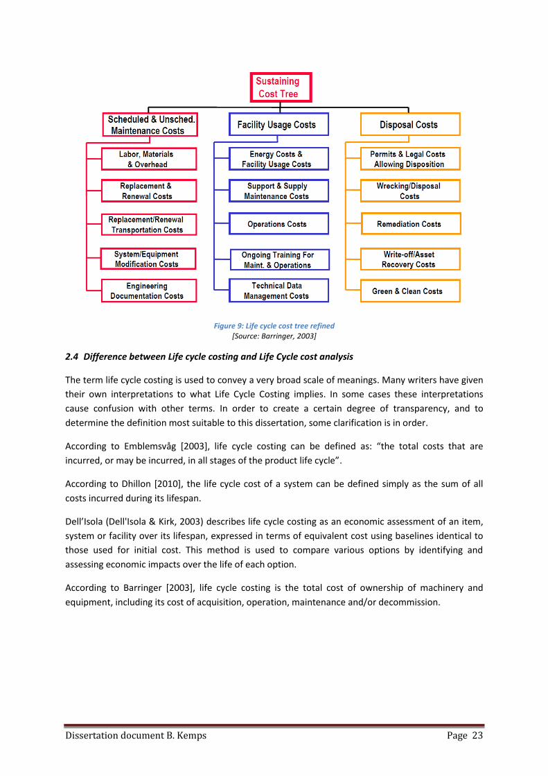
Dissertation document B. Kemps Page 23
Figure 9: Life cycle cost tree refined
[Source: Barringer, 2003]
2.4 Difference between Life cycle costing and Life Cycle cost analysis
The term life cycle costing is used to convey a very broad scale of meanings. Many writers have given
their own interpretations to what Life Cycle Costing implies. In some cases these interpretations
cause confusion with other terms. In order to create a certain degree of transparency, and to
determine the definition most suitable to this dissertation, some clarification is in order.
According to Emblemsvåg [2003], life cycle costing can be defined as: “the total costs that are
incurred, or may be incurred, in all stages of the product life cycle”.
According to Dhillon [2010], the life cycle cost of a system can be defined simply as the sum of all
costs incurred during its lifespan.
Dell’Isola (Dell'Isola & Kirk, 2003) describes life cycle costing as an economic assessment of an item,
system or facility over its lifespan, expressed in terms of equivalent cost using baselines identical to
those used for initial cost. This method is used to compare various options by identifying and
assessing economic impacts over the life of each option.
According to Barringer [2003], life cycle costing is the total cost of ownership of machinery and
equipment, including its cost of acquisition, operation, maintenance and/or decommission.

Dissertation document B. Kemps Page 24
When using life cycle costing to compare different alternatives, one should be aware that not all cost
categories are relevant to all projects. The preparer is responsible for the inclusion of the pertinent
cost categories that will produce a realistic life cycle costing comparison of project alternatives. If
costs in a particular cost category are equal in all project alternatives, they can be documented as
such and removed from consideration in the life cycle costing comparison. [Mearig, Coffee, &
Morgan, 1999] Dell’Isola and Kirk [2003] also mention that costs that are considered to be the same
for all alternatives can be eliminated from the life cycle cost analysis.
Thus, life cycle costing can be used as a method to compare and analyse different alternatives. When
comparing different alternatives it is possible to remove equal costs from consideration. If costs are
eliminated from consideration, one must be aware that the definitions of life cycle costing
mentioned above are no longer appropriate: when costs are eliminated from consideration it is more
suitable to use the term life cycle cost analysis (LCC analysis).
Life cycle cost analysis can be described as a cost-centered engineering economic method whose
objective is to systematically determine the costs attributable to each of one or more alternative
courses of action over a specified period of time. The key elements of such an analysis will be
examined, as will be the effectiveness of its results in a particular situation.
Before starting the process of cost calculation, it is important to clearly determine what exactly is to
be investigated.
Life cycle cost analysis can be used as a method to compare different alternatives.
Life cycle costing can be used to gain insight in the total cost of ownership of an asset.
It is important to keep this in mind when using a life cycle cost analysis model.
In addition, it is to be noted that when some equal costs are removed from the comparison, it is not
easy to reimplement these specific costs at a later stage. During the time that has lapsed, costs may
have changed, resulting in increasing inaccuracy of the outcome. It is also to keep in mind that
initiating and going through the process again is time-consuming. This can be of importance when,
for instance, a third or fourth alternative becomes possible. This problem also occurs when, at a later
stage, the management decides to investigate the possibility of investing in a complete new
installation. When costs are eliminated from consideration it will be hard to compare this
investigation with the life cycle cost analysis made earlier, because the latter is incomplete.
2.5 Area of interest in LCC analysis
For this particular case study, the pilot company can be seen as the purchaser and user of a new
asset/installation. This means that the customer perspective is most suitable for the pilot company.
Figure 10 below shows the area of interest for this business case. It visualizes the fact that the life
cycle cost analysis of the manufacturers is not taken into account. The different options available to
the manufacturers, and their specifications, are simply the input parameters of the analysis. For the
disposal of the installation it is important to know what the cost or perhaps residual value will be, as
expressed in euros.

Dissertation document B. Kemps Page 25
Figure 10: Area of interest in LCC analysis for the pilot case [Source: B. Kemps]
In this chapter, the scope of LCC analysis for the case study has been defined. A customer perspective
is most suitable, which implies that the development of installations is not of primary concern. The
purchase of the installation can therefore be seen as an input parameter. Further research has
pointed out that it is not necessary to conduct a complete LCC calculation. A life cycle cost analysis is
sufficient to investigate the case study.

Dissertation document B. Kemps Page 26
3 Models
3.1 Introduction
In this chapter, an impression of commonly used LCC models will be given. Directly linked to these
generally known models, a model suitable for this particular study will be presented. Shortcomings
will be pointed out; if possible, the model will be adapted with regard to these specific areas of
interest.
3.2 Commonly used models
In literature, life cycle cost models are described. Theories regarding these models are mainly
described in general. The models have become more and more elaborate and their complexity has
increased over the years. An abstract of the most important references relevant to this research will
be given below.
This thesis is part of the master’s program in “Asset Management Control” (AMC). The field of
interest within this AMC study is to improve cost-effective management of capital assets. Many
companies exploiting capital assets have to deal with identical problems related to the following
AMC objectives:
Specify system functionality
Acquire system functionality
Achieve cost-effectiveness
To meet these objectives, the AMC domain focuses on five specific areas of interest, viz.
management, engineering, education, information, and communication throughout the life cycle of
an asset. A Life cycle management (LCM) approach has been designed to meet these objectives.
In the figure below, the domain within this LCM approach is visualized.
Figure 11: Life Cycle management domain [Source: Stavenuiter, 2002]

Dissertation document B. Kemps Page 27
The Life cycle management domain mentioned above consists of different stages. In all of these
stages, different kinds of data are needed. All this data is collected, structured and provided by
Product Data Management (PDM). The total data needed to manage capital assets is called a life
cycle management (LCM) data set.
A considerable amount of parameters – including operating requirements, reliability, availability,
maintainability, energy, maintenance plans, etc. – is needed for an LCM data set and for life cycle
cost calculations. As such, a life cycle management data set can provide all data needed to make
proper cost calculations. Stavenuiter [2002] has developed a model to manage complex assets such
as marine ships. The model is able to visualize the effect of different installations and actors in terms
of performance of the total system. As Barringer [2003] points out, the purchase of the installation
can be seen as acquisition costs. Only slight specific adjustments of the installation are sometimes
possible. For this reason, the installation will usually be produced after an agreement on the
specifications. This is visualized in figure 12 below. Mainly relevant to this investigation are the
differences in costs of utilization and maintenance. As becomes clear, the LCM model deals with
many more aspects than is necessary for this thesis.
Figure 12: LCM, simplified for the purposes of this master thesis [Source: Stavenuiter, 2002]
However, the model itself will not be used, because it is too broad to be used directly for life cycle
cost calculations for SMEs. The general approach and insight gained into Life Cycle Management (and
AMC), however, has been very useful.
Fabrycky and Blanchard [1991] introduce three different ways to estimate costs:
Cost estimating by engineering procedures
Cost estimating by analogy
Cost estimating by parametric estimating methods.
Emblemsvåg [2003] also mentions these ways of cost estimating, describing them as models, and
adds a fourth way to estimate costs, viz. cost accounting models.
Cost estimating by procedures, (engineering cost models according to Emblemsvåg)
Costs are assigned to each element at the lowest level of design detail and then combined into a
total for the product or system. The main difficulties with this method are the need for detailed data
and the efforts involved in performing the calculations.

Dissertation document B. Kemps Page 28
The basic idea of Estimation by Analogy is to create accurate estimates for new projects by
comparing the new project to similar projects from the past. The most significant problem of this
type of estimating is the high level of judgment required. It is the cheapest way of cost estimating,
because not much data is needed.
Parametric estimation utilizes different statistical techniques and seeks for the factors on which the
life cycle cost depends. This type of estimating requires a lot of data. Emblemsvåg [2003] explains
that parametric models are in many ways more advanced analogy models.
The fourth cost estimating model, according to Emblemsvåg [2003], is what he calls cost accounting
models. He analyzed this way of cost estimating into three groups:
Volume based costing
Unconventional costing
Modern cost management systems
Cost management systems are frequently discussed in the literature. Emblemsvåg describes four of
them: Activity Based Costing (ABC), Just In Time (JIT) Costing, Target Costing (TC) and Strategic Cost
Management (SCM).
In addition to these models, he has developed an approach of his own in which he combines the
benefits of activity-based costing, life cycle costing and Monte Carlo methods. It results in a model
with a lot of advantages over the existing models.
Activity-Based life cycle costing handles both costs and cash flows
Activity-Based life cycle costing is process-oriented
Activity-Based life cycle costing relies on the establishment of cause and effect relationships
Activity-Based life cycle costing handles overhead costs
Activity-Based life cycle costing estimates the cost of all cost objects of a business unit
simultaneously
Figure 13: Three layers of activity-based life cycle costing [Source: Emblemsvåg, 2003]
Activity- Based Costing
•Overhead costs
•Relevant cost assigment
•Cause and effect
•Multiple cost objects
•Process-orientation
•Cost vs expense
•Cost vs cash flow
•Links to TQM, EP
Life-Cycle Costing
•Life-cycle perspective
•Total costs
•Cashflows
•Discountingfactors
Monte Carlo Methods
•Statistical sensitivity analysis
•Handle risk and uncertainty realistically
•Large models
•No limits

Dissertation document B. Kemps Page 29
3.3 Models relevant to this study
The question arises whether such complex approaches make sense for SME companies with an
established market and standard production equipment. As discussed before, the best way to
describe the life cycle of investments within these types of companies is the costumer perspective.
The key question for these companies will be “how to reduce costs” or, formulated in a slightly
different way, “what alternatives of an investment will be the one with the least incurred costs”.
With this in mind, all costs which are equal for the alternatives can be disregarded.
Dell’Isola [Dell'Isola & Kirk, 2003] describes a model disregarding all equal costs. Only costs that are
different for the alternatives will be included. For this reason, most life cycle costs can be
disregarded, which makes the model concise, clear and easy to understand. The advantage of less
input parameters is that it makes the relationship between outcome and input parameters much
easier to demonstrate.
The model provided by Dell’Isola [Dell'Isola & Kirk, 2003, cf. appendix 1] is based on an Excel
spreadsheet: this makes the model very accessible and, in addition, adaptable to specific cases. What
is more, this makes it possible to combine the model with other Excel based models. The latter
possibility will be drawn on in section 3.6, where the model will be extended through an uncertainty
and sensitivity analysis.
Dell’Isola distinguishes three types of costs (cf. appendix 1):
Initial/ collateral costs
Replacement/salvage costs
Annual costs
This classification is mainly based on the moment when and frequency with which the costs occur. As
a result, the classifications have their own ways of dealing with the value of money in time. This will
be discussed in section 3.5.
3.4 Cost breakdown structure
To make this model useful for this study, it is first of all necessary to examine the costs involved. An
inventory has therefore been made of all the costs of the life cycle of the assets. This is called a cost
breakdown structure. When grouping the major cost categories, it is useful to estimate all applicable
costs for each category. Besides the inventories and price level of the costs, it is also important to
investigate the frequency over its lifespan. With regard to this research, it is to be noted that not all
costs have to be investigated. Because, as stated before, this is an analysis of different alternatives,
costs that are similar in each alternative may be deleted from consideration. [Blanchard, 2004]

Dissertation document B. Kemps Page 30
For the purposes of this study, the following cost breakdown structure is used:
Initial/collateral cost
A. Purchase
B. Training
C. Support tools (tools exchangeable with other assets)
Replacement/salvage cost
A. Replacement costs hardware (technical lifespan)
B. Update software (including training)
C. Spare parts
D. Disposal/demolishing
Annual costs
A. Maintenance
B. Failure costs
Repair costs
Downtime costs
Disposal/residues
C. Requirements
Energy
Air
Extraction
Heating
D. Personnel
E. Downtime changeovers
3.5 Discount and Escalation rate
To make future costs comparable to today’s costs, it is necessary to incorporate both a discount rate
and an escalation rate. In the literature, much has been written on discount rates and methods
available for determining them. There is no universally accepted method or resulting rate. The
discount rate is often described as “the minimum attractive rate of return” on an investment. It is
generally the prerogative of the owner or policy maker to select the discount rate. The rate usually
includes the basic cost of borrowing money plus an increment that reflects the risk associated with
the investment. [Dell'Isola & Kirk, 2003] In appendix 2, formulas are given to calculate the present
worth factor and the present worth of annuity factor. These factors have to be used because today’s
euros will not necessarily have the same value tomorrow (appendix 3, effect of discount rate). Future
costs, such as operation and maintenance costs, have to be discounted to their present values before
they can be compared with such items as acquisition or procurement costs. On the other hand, some
costs will increase over time. Energy costs have become higher and higher, but labour costs are not
constant either. For that reason, an escalation rate should also be used. As opposed to the discount
rate, the escalation rate will be specific for the different types of costs. With the discount and
escalation rate, it is possible to determine the present worth factor (appendix 2).

Dissertation document B. Kemps Page 31
3.6 Uncertainty and sensitivity
The need for uncertainty assessments comes from the fact that input data for an LCC analysis are
based on estimates rather than known quantities. The data input is, therefore, uncertain.
Uncertainty exists in all situations when things are unknown, unpredictable, open-ended or complex.
Emblemsvåg [2003] defines uncertainty as a subset of unpredictability, which in turn is a subset of
the unknown. He states that an uncertain matter is not unknown or unpredictable. The problem is
the lack of information and knowledge about it. In addition, uncertainty is best described in relation
to complexity. This complexity often arises in open systems because they interact with their
environment to various degrees and evolve over time.
To identify high cost distributors, a sensitivity analysis can be conducted. A sensitivity analysis
examines the impact of changes in input parameters on the result. Varying the input parameters over
a range to see the impact on costs can help to highlight the major factors affecting costs. With a
sensitivity analysis it also becomes possible to visualize the effects on costs of different design
possibilities.
Different methods for conducting a sensitivity analysis have been developed. In this case the Monte
Carlo simulation will be used. This is a statistical method that involves the use of regression and
related partial correlation coefficients. It can be described as a statistical method that simulates what
happens in the model for a certain quantified number of points. The end result will not be exact, but
it will be good enough to give reliable indications. This simulation method can handle complicated
systems with many parameters. An advantage of this simulation is that it simultaneously combines
both a sensitivity analysis and uncertainty. The Monte Carlo simulation enables one to introduce
uncertainty in the model’s input variables in order to measure statistically the impact this uncertainty
has on the output’s variables.
The program @Risk will be used to perform this Monte Carlo simulation. In lectures on LCC as part of
this master’s program, the advantages of this tool became clear. It is a program/tool that uses
Microsoft Excel to perform this analysis. It can be completely integrated into the spreadsheet used.
The program is able to run Monte Carlo simulations; it recalculates the spreadsheet model thousands
of times. Based on the random values from the @RISK functions that are entered, it samples/changes
the input data, after which the program records the resulting outcomes. The resulting outcomes of
the simulations can be visualized by different graphs.

Dissertation document B. Kemps Page 32
4 The purchasing process
4.1 Introduction
In the previous chapters insight is gained on the scope of LCC analysis and what input parameters are
needed to perform a decent LCC analysis regarding this thesis. In order to improve the purchasing
process of assets it is necessary to have a correct impression on the current policy of purchasing
assets. There must also be clarified what data is at hand and how this data is provided. When this
information is known, it becomes possible to point out expected improvements with the contribution
of LCC analysis. So in this chapter sub questions 4 and 5 will be handled.
4.2 Purchasing policy of SMEs
SMEs often lack unambiguous or clearly stated policies for purchasing new installations. The demand
for an investigation into the possibilities of changing or expanding certain processes is usually caused
by:
Obsolescence of the current installation
Problems regarding capacity
Newer and improved production processes
Higher demands of regulatory rules stated by government or branch organizations
Exploration of new markets requiring new installations
These motives can/will lead to investigations into the most suitable alternative solution to meet the
requirements. The next section describes the purchasing process common to many SME companies.
It is based on Veteka (appendix 6). The case studies as described in section 5 are also based on this
company.
Generally the management team is responsible for the purchase of a new installation. When a
certain demand is signalized, they will start exploring the different possibilities.
When it concerns an existing installation they will investigate the possibilities for updates and a
complete overhaul. Usually this specific part of research is not very time-consuming, because of the
age of the asset concerned. The asset is usually outdated to such an extent that investing in a
complete overhaul and updates is simply too expensive. To come to this conclusion they mainly rely
on their own expertise. When there is some doubt about the feasibility of a certain overhaul or
update in relation to a complete new installation, they just make a phone call to one of their
suppliers for some indicative price settings. In those cases it is very easy to conclude whether or not
further investigation is advisable.
When the decision has been made to investigate the feasibility of a new installation, a list of
requirements will be set up. Every person who will become directly involved with the new
installation has the possibility to share his findings and recommendations. All items of this list will be
evaluated and they will be given a priority level. This list will be discussed with the board of directors
so all parties are aware of what is expected.

Dissertation document B. Kemps Page 33
Because the technical lifespan of installations often exceeds twenty years, the management typically
prefers a supplier that can be trusted and is consistent. For this reason the board of SMEs prefers to
choose well-known and recommended brands. So they make a first selection based on experience
and brand of potential suppliers which they contact for an appointment to discuss the plans and
requirements. They listen to their ideas and perspective on the situation.
Agreements for a first offer are made. These offers are collected. The management individually
studies and compares them. When all offers have been looked into, the management and all internal
parties involved sit together to discuss and compare the different alternatives.
Offers which are obviously unable to meet the requirements are dropped. In those cases, the
representative is informed. He often requests a final chance to review his proposal. When he is able
to convince the management that his company can meet the requirements, the management gives
him this last chance. Meanwhile, negotiations with other representatives continue.
In practice, negotiation is an ongoing process, in which comparisons are made and details discussed.
In some cases, but not always, the different options are compared in an overview made in Excel. To
investigate the revenues a small calculation is made on paper or in Excel. The purchasing process is
very flexible and based on expertise.
As should be clear from this description, there are no specific rules and guidelines. Decisions are
mainly based on feelings, trust, and experience. Because of the long term relationships between the
company and employees and employees and suppliers, a considerable amount of specific knowledge
is available. This can be seen as one of the company’s strengths.
During the last 15 years, however, there has been a revolution in the implementation and
combination of new technologies, including electronics and computers. [Emblemsvåg, 2003] This has
also affected the timber industries. In addition, the technological revolution in countries like China,
Korea and Taiwan has led to a new outlook on the purchasing process. Nowadays many “new”
constructors from foreign countries have proved their existence. Some of them have already existed
for more than 20 years and in most cases they are still growing every year. They have been able to
set up a dealer network, with a complete supporting service in Europe. A faster changing technical
environment and the emergence of new brands have led to a change in our familiar and safely
trusted environment. The existence of new makes and faster developing technologies can therefore
no longer be ignored. In future, these developments will have to be taken into account during the
purchasing process.
4.3 Reliability, availability and maintainability of current installations
Reliability can be defined simply as the probability that a system or product will perform in a
satisfactory manner for a given period of time when used under specified operating conditions.
There are four key elements which are extremely important when determining the reliability of a
product/system or asset:
Dissertation document B. Kemps Page 34
1. Probability: this is usually stated as a fraction or a percentage signifying the number of times
that an event occurs, divided by the number of trials.
2. Satisfactory performance: this is usually presented in the specification of a system that is
required. It concerns qualitative and quantitative factors.
3. Time: this is one of the most important elements when determining reliability. For a
particular function one must be able to predict the probability that an item will survive
(without failure) for a designated period of time. Often the reliability of a system is defined
as the Mean Time Between Failure (MTBF), Mean Time To Failure (MTTF) or Mean Time
Between Maintenance (MTBM).
4. Specified operating conditions: these are the conditions in which the system/product or asset
must be able to operate. These conditions include environmental factors, such as humidity,
temperature, vibration, etc.
Availability: within the context of systems engineering, availability can be defined as a measure of
system readiness. It can be expressed as a probability that an item or system is in an operable state.
In most cases, the probability is expressed as a percentage.
Maintainability: maintainability is the ability of an item to be maintained. It can be defined as a
characteristic in design that can be expressed in terms of maintenance frequency factors,
maintenance times and maintenance costs. Maintainability is a design parameter. A system should
be designed in such a way that it can be maintained without large investments of time, cost, or other
resources.
The maintenance itself includes all actions necessary for retaining a system or product in, or restoring
it into, a serviceable condition. Maintenance can be divided into two categories, viz. corrective
maintenance and preventive maintenance.
Reliability and maintainability have a huge impact on the success of the system in fulfilling its
intended purpose. When designing or implementing a new installation it is therefore important be
aware of the characteristics that affect reliability and maintainability.
An analysis of reliability, availability and maintainability together can be defined as a RAM-analysis. It
is typically used to predict the performance of processes and systems and to provide a basis for the
optimization of such systems. In such analyses the key performance indicator is availability, which is
the fraction of time that the system is fully functional. The purpose of this analysis is to investigate
and point out those items that have the greatest effect on availability. Afterwards it becomes
possible to carry out further investigation into those items in order to redesign certain aspects to
optimize the performance of the installation. [Blanchard, 2004]
In SMEs, data collection regarding availability and reliability of installations is scarce. Information can
only be derived from the maintenance that has been done on a certain installation in the past. Thus,
maintenance is assessed for each installation separately. In addition, these two aspects are evaluated
based on expertise and feelings. If an installation becomes unreliable or availability becomes critical,
the people in charge will determine what the exact problem is. Therefore, performing a reliable
RAM-analysis is often impossible.

Dissertation document B. Kemps Page 35
4.4 Improvements expected from implementing LCC analysis
One of the stated sub questions is to list expected improvements which will result from
implementing an LCC analysis. The current purchasing process has been described in paragraph 4.1;
with the theory which has been reviewed, the following outcomes are expected.
An LCC analysis is a data based decision making approach. When parameters are correctly fulfilled, it
generates hard decision making data. It makes it much more difficult for stakeholders and
management to doubt whether the right decision will be made. In addition, it also can help to
convince banks to lend money for the project at hand.
Because LCC implies that all cost drivers are taken into account, it is to be expected that a number of
hidden costs will emerge from the analysis.
With the program @risk, it is possible to determine the uncertainty and sensitivity of the different
input parameters. The outcomes on the uncertainties and sensitivities can result in new perspectives
and possibilities in order to reduce the uncertainty, sensitivity and the scale of the total costs.
It is to be expected that when, through the implementation of LCC, hidden costs emerge which have
to be taken into account during the purchasing process, more cost-effective alternatives will win out
on the traditional purchasing process.

Dissertation document B. Kemps Page 36
5 Cases
5.1 Description of the cases
In order to test the hypothesis, four life cycle analyses have been investigated. A description of the
cases will be given in this chapter. All these cases are practical examples from the company Veteka
(appendix 6). In the next chapter, the relevant analyses will be described and the results will be
discussed.
5.1.1 Weinig versus Leadermac
When different aspects of the pilot company, Veteka, are analyzed, it is clear that high standards are
applied throughout. Veteka’s policy has always demanded high quality installations. As described
earlier, some new makes have entered the world with relation to the purchasing process. These
makes are often a lot cheaper than the traditional, well-known brands. Because they have proved
their existence, the management can no longer ignore them. For this reason, this study will use LCC
to compare alternative moulders.
Traditional moulders at the pilot company have been made by two companies, Weinig and Waco.
About 7 years ago, Waco has been taken over by Weinig. The two brands still exist, but technologies
and price settings have been mutually adapted. The dealer for these brands is De Groot, located in
Rosmalen. An upcoming brand of moulders in Europe is “Leadermac”. The company is located in
Taiwan. The first time this brand crossed Veteka’s path was about 10 years ago at a trade fair in Italy.
On each fair the management visited, the expansion of the brand “Leadermac” was noted and, over
the years, the technical possibilities of its machinery have continuously grown. The dealer for
“Leadermac” in the Netherlands is VOS, located in Hendrik-Ido-Ambacht and not unfamiliar to
Veteka. VOS previously dealt for Waco but, due to the take-over of Waco by Weinig, lost his
dealership for the company.
In the first case a moulder from Weinig will be compared with a moulder from Leadermac. To
conduct this analysis information has been requested from the dealers.
5.1.2 Moulding Cutter Head
A few years ago a new moulder was purchased. De Groot in Rosmalen was contacted with a view to
purchasing a new Weinig. The requirements concerning possibilities, variations and options were
made clear. Weinig’s factory (located in Germany) was visited twice, with a view to clearly discussing
and looking into the different alternatives. This also applies to a new system used for the moulding
cutter head, “the Weinig Powerlock Cutter Head”. The main advantages of this system are the
reduction of exchange times and the higher routes per minute of the knives, resulting in a higher
linear meter capacity.
The management decided not to purchase this new technology for two main reasons:
The technology was brand new in the timber industries at that time. There was only practical
experience at the Weinig factory. The results of the demonstration given were perfect.
However, on Veteka’s side, there were doubts about the locking system. It had not yet
proven its worth in a production environment.

Dissertation document B. Kemps Page 37
Veteka possesses 4 moulders. All these moulders can be fitted with the same tools. When
the decision had been made to choose the Power lock system, it meant that a complete new
set of tools had to be purchased as well. Moreover the tools for this new moulder wouldn’t
be interchangeable with the other moulders. If the new asset with a Power lock system
failed, a tool could not be used on the older moulders. The result would be that delivery
times promised to customers would not be met, especially if the tool was specially
commissioned.
A third, but less important issue was the price setting of the Power lock system. The decision to
choose the traditional way of clamping the tools, then, was based on feelings.
Today, the Power lock system has given clear proof of its quality. Many customers of Weinig chose
this option and, as far as is known, there are virtually no complaints. An LCC calculation will be set up
to investigate whether the Power lock system would have been worthwhile.
Figure 14: Power lock system versus traditional moulding cutter head [Source: http://www.weinig.com/Internet/weinig_base.nsf/CurrentBaseLink/W26AYRZ8000LUNAEN]
5.1.3 Coating line
Most wooden profiles are coated before they leave the factory, either with a prime coating or with a
complete finished surface. This reduces the amount of work on the construction site itself. The
standards for applied coatings are continuously raised to a higher level in thickness, smoothness,
colour, endurance, etc.
A few years ago, Veteka began to investigate the different possibilities for a new coating line. The
current coating lines are out of date and, as described earlier, the market demands a higher standard
of coatings. When investigating the suitability of alternative coating lines, the management
considered two options. Generally, these systems are highly similar: both consist of two vacuum
coaters and two drying tunnels. The main difference is the transport system of the products
(plinth/strips). Traditionally, the products go through the vacuum coaters and, by means of a
transport band and chains, through the drying tunnel. Then, at the end of the tunnel, they have to be
handled manually in order for a second (or third) coating to be obtained if necessary, or in order to
be packaged. The alternative system uses a sophisticated transport system and two vacuum coaters
in line. The advantages of this system are:

Dissertation document B. Kemps Page 38
A reduction in labour costs; the manpower used at the end of the first installation is no
longer needed.
Because of the sophisticated transport system, the coatings will hardly be damaged during
the process. This makes it possible to get a layer of 100 mµ in one production run (i.e. twice
through a vacuum coater). Traditionally, three runs would be needed to achieve this,
because of damage caused by the transport chains.
Not all costumers, though, will necessarily ask for a high end product with a 100 mµ layer. Thus, in
most cases one or two runs through a vacuum coater will suffice.
It is clear that the alternative system, with its sophisticated transport system, has higher initial costs.
It may also be a matter of discussion whether this system might not be less flexible than the
traditional system, and more prone to failures. Moreover, it may be said that if any failure occurs, the
complete coating division will be down.
A life cycle costing analysis will now be made in order to compare these two alternatives. A couple of
assumptions will have to be made about the input parameters, which will substantially influence the
results. This will be discussed in the next chapter.
Figure 15: Layout new coating line [Source: Internal information: Makor offer]

Dissertation document B. Kemps Page 39
The main difference between the two options is located at positions A. Here, it is possible to choose between a relatively standard installation or a more custom-made alternative. The advantage of the alternative solution is that transportation does virtually no damage to the wooden profile. Since the backside (downside when in the transportation system) will have enough lacquer on it, it becomes possible to guarantee 100 microns of dry lacquer in two runs.
Figure 16: Sophisticated transport system [Source: Internal information: C-Tech offer]
5.1.4 Double vacuum box
One possible way to coat wooden profiles is by using a vacuum coater. The coating application uses a
vacuum system. The application itself takes place in a small box. The wooden profile enters and exits
this small box by means of a contra profile which follows the contours of the wooden profile. Inside
the box a vacuum environment is created, and paint is injected on the wooden profile. When the
profile exits the box, the paint will be sucked from the profile. The feeding speed of the wooden
profile, the amount of suction and the clearance between wooden profile and contra profile together
determine the amount of lacquer that remains.
Due to higher market demands, more and more colours changes have to be made during the day.
This implies that the vacuum installation needs to be cleaned. This cleaning process is time-
consuming, which results in a reduction of the daily production capacity. However, Schiele, for
instance, has made it possible to simply change the vacuum boxes in which the application takes
place. Thus, the paint can remain in one box. By simply removing this box from the production line
and replacing it with another box with a different colour, it becomes possible to reduce the halt in
production to almost zero. Nevertheless, at the end of the day, all vacuum boxes will have to be
cleaned in order to serve the next day.
A life cycle cost analysis will be made to compare these two alternatives.

Dissertation document B. Kemps Page 40
5.2 Input parameters
5.2.1 Starting points
Before looking at the individual cases themselves, some common parameters can be discussed.
These will be equal in all cases.
Lifespan
It must be clear which period is taken into account. The longer the lifespan, the higher the risk that
several parameters become inaccurate. To reduce this inaccuracy, a specific lifespan for each case
will be chosen. For example, will the labour or energy costs which are the escalation factors involved
be constant over the next years (thus showing linear growth), or might the economy or environment
change in such way that they create a situation in which those factors cannot be seen as constant?
Discount rate
As discussed before, the discount rate of a specific period can be set at the same value for all assets
relevant to this study. However, this rate greatly influences the outcomes of life cycle costing. A high
discount rate results in future costs being of minor influence. Barringer [2003] used a discount rate of
12% as common, not very high or low. In this case a rate of 9% is used. This may be relatively low but
interest at this moment is historically low and since the company is financially very strong, a low
interest rate is possible. In the conclusion to this case study, an investigation will be made into what
the result of a higher or lower discount rate would be.
Unlike the discount rate, the escalation rate will be specific for every case; indeed, it will characterize
every item in a single case. The escalation rate will therefore be discussed for every distinct case.
Disposal
During the lifespan as well at the end of the lifespan (either demolishing the installation or taking the
rest value of the installation into account) the cases have to deal with disposal (residues of the
production process). Both items can easily be translated into costs which will be defined for the
different cases.
5.2.2 Manufacture parameters
As described in section 2.2, the input for the LCC analysis will be the manufacture parameters of the
installations of the different alternatives (figure 16).

Dissertation document B. Kemps Page 41
Figure 17: Manufacture parameters [Source: B. Kemps]
Some of these parameters are directly related to costs (e.g. the price of an installation); others have
no direct link to a specified amount of money. Where the latter parameters are concerned, a
conversion has to be made to an equivalent of costs for the parameter involved. For some
parameters, this may be difficult, and a lot of assumptions will have to be made. For such a
parameter as quality, for instance, this will result in maintenance costs, failure costs and replacement
cost (for either parts or a complete installation).
These conversions can be specific for each case. It may also be possible to eliminate some of the
parameters in the cases described, since these parameters result in the same costs for the different
alternatives. For this reason, these parameters have to be examined case by case in order for the
correct equivalent of costs to be reached.
Finally, not all manufacture parameters will have to be converted into costs. Some parameters are
(minimum) requirements that have to be met by the installation. Such parameters as capacity,
precision, proportion or options are examples of such hard requirements. They may influence the
(purchase) price of the installation, but will not lead to additional costs.
5.3 Results
For all cases discussed, a life cycle cost analysis has been set up, as explained in chapter 3.4. Input
parameters were defined using the cost breakdown structure and Dell’Isola’s Excel sheet (appendix
4). The output of the model results in the life cycle cost present worth difference. This output
parameter indicates whether an alternative is interesting or not.
This has been done for every individual case. To examine the influence of some parameters on the
output, graphs were made with curves plotting the life cycle cost present worth difference against
the lifetime for different input parameters, with one parameter being changed every time. The
advantage of this simple way of conducting sensitivity analyses is transparency, and the fact that it is
easy to understand for everyone. From these graphs, it became clear that the choice of discount rate
greatly influences all cases.

Dissertation document B. Kemps Page 42
To improve this simple but arbitrary way of conducting sensitivity analyses Dell’Isola’s Excel sheet has
been modified in such a way as to make it possible to import @Risk in the model. For each of the
input parameters a distribution has been defined (cf. input parameters, appendix 4). When the
models are approached by means of a Monte Carlo simulation, this results in a mean output
parameter and the standard deviation of this parameter. @Risk also gives the correlation coefficient
of each input parameter with the output parameter.
Appendix 5 shows the results of the four cases. A description of the different graphs is also given.
5.3.1 Weinig versus Leadermac
The main difference between Weinig and Leadermac is the price of purchase. This can be derived
from appendix 4.1. Both moulders have the same specifications and are in that respect comparable.
Since Leadermac is expected to be of a minor quality, a technical lifetime of 15 years is expected. The
lifespan of a Weinig, by contrast, will, after an update, be ten years longer.
The influence of the replacement cost of a moulder (at 15-25-30-40-45 years), is clearly seen in
Appendix 5.1, graph 1. In order to clearly visualize the impact of the different lifetimes of the assets,
a lifetime of up to 75 years is examined, which will smoothen the effect over time. It is obvious that
this does not correspond to reality. The complete calculation is shown in appendix 4.2.
The results of the Monte Carlo simulations (cf. appendix 5.1, graph 3 specifically) show, that with a
lifespan of 25 years, the discount rate influences the results the most. This makes sense, since the
longer the lifetime, the more the influence of the value of money in time will increase.
As all graphs show, the Leadermac is expected to cost slightly less than the Weinig. The question
arises whether the difference is significant enough to opt for the Leadermac. In this case, positive
experience with Weinig in recent years may be expected to tip the balance in favour of the latter.
5.3.2 Moulding Cutter Head
By the second case, the investigation had to be modified. The Powermat Cutter Head was not
compatible with our current moulder, so a fair comparison was impossible. Weinig has a special
product line for the Powermat Cutter Head which is lower in price, but has fewer possibilities.
However, the case remains an interesting one: if the Powermat line turns out to be suitable for the
company, an overkill of capacity and opportunities with the current moulder (the Hydromat 2000 of
the High-speed line) may be possible. In that case, Veteka could have saved on purchase, labour cost
and energy cost by purchasing a moulder of the Powermat line. Although this is a very interesting
question, another way has been chosen to transform the second case.
Leadermac can provide the Speedmac (counterpart of the Hydromat) with an HSK clamping, which is
equal to the Powermat cutter head. This HSK clamping gives an additional cost of € 7.500 for each
axis. Within the company’s production process only five of the seven cutter heads are changed
frequently, so a Leadermac with traditional cutter heads will be compared with a Leadermac with
five HSK clamping systems. Besides the additional cost of the clamping system, extra costs have to be
taken into account for training, and since the traditional cutter chisels do not fit onto the new
system, an additional cost for support tools will be necessary.

Dissertation document B. Kemps Page 43
Appendix 4.4 shows the Excel calculation sheet for this particular case. Besides the additional costs of
purchasing the Cutter Head, there will be a reduction of changeover times. As is clearly visualized by
the results from the Excel sheet (appendix 4.4) and the distribution (appendix 5.2, graph 6), the HSK
clamping system will hardly yield any savings for the parameters chosen. Changing these parameters
demonstrates that the influence of changeover times is enormous, as shown in appendix 5.2 graph 5,
“Reeks 2”.
The Monte Carlo analysis confirmed this simple sensitivity analysis: as shown in graphs 7 and 8
(appendix 5.2), changeover times had the highest correlations in uncertainty and sensitivity, followed
by discount rate. Clear insight into the changeover times is therefore essential.
5.3.3 Coating line
In the case of the coating line, the additional cost of the sophisticated line is the highest amount of
money. Added to this is the fact that the sophisticated line has a higher failure cost during the first
two years and it is expected to need updates after 5 and 15 years. There will, however, be savings in
energy, heating and labour costs (appendix 3). These parameters are all processed in the Excel sheet.
The simple method (appendix 5.3, graph 9) shows that in the long term the sophisticated line will win
out on the traditional line. For a low discount rate or by coating more meters this effect will be
stronger.
From the Monte Carlo analysis, it can be concluded that there is a high degree of uncertainty in the
result (appendix 5.3, graph 10). To further refine this, a better estimate of the amount of meters per
day and/or the escalation rate of the labour cost is necessary, as is shown in graph 11.
5.3.4 Double vacuum box
In the fourth case, it may at first seem that there is only an additional cost at the time of purchase,
with no additional profits. The work of cleaning the vacuum boxes is the same for both options. So, at
first sight, the double vacuum box is less attractive. But when the production process is taken into
account, it turns out that secondary costs are also involved: in the single version, when the vacuum
box is being cleaned, the entire production line will have no output. Yet the heating and ventilation
of the drying chamber and the transport system will still be running. In the case of a double vacuum
box, these cost are eliminated.
So the benefits of a double vacuum box are lower energy and heating costs. When calculating these
costs, one may be surprised at the amount to which they add up on an annual basis. (For the
complete layout see appendices 4.7, 4.8 and 5.4.)
The Monte Carlo analysis also shows that discount rate has a considerable influence in this case.
While the discount rate creates the highest degree of uncertainty, the model is most sensitive for
energy costs (appendix 5.4 graph 15 & 16).

Dissertation document B. Kemps Page 44
5.4 Conclusions to separate cases
The first case proves that even with a technical lifespan which is presumed to be 10 years shorter
than that of a Weinig, the Leadermac is still more cost-effective. Based on the data yielded by LCC
analysis, which will have to be taken into account, a future purchase of this “new” make is
warranted. With the right input parameters, it is possible to provide conclusive proof of which of the
two (or more) alternatives will be the most advantageous. This method provides the management
with objective and, moreover, understandable data, which can replace the feelings, trust and
experience of the human being.
The existing uncertainty in the results for case 1, case 3 and case 4 is influenced most by the discount
rate, as can be derived from graphs 3, 11 and 15. A large amount of uncertainty increases the
probability that the wrong decisions will be made. In order for proper and well-founded decisions to
be made, it is therefore essential to reduce this uncertainty. To do so, specific further investigation
related to the discount rate will have to be carried out.
Case 4 and case 1 visualize the differing impact of energy costs on the alternatives over the course of
several years. Because these costs would never have been assessed without LCC analysis, the energy
costs involved may be termed “hidden costs”. Furthermore, case 4 clearly shows the advantages of
doing an LCC analysis. Because the investment was relatively small, and savings in terms of efficiency
cost were unknown, but little attention was spent on this case. The result, however, shows that
investing in a double vacuum box system is highly likely to have a positive outcome. This can be
deduced from the distribution, which is relatively small, and is nearly always positive (appendix 5.4,
graph 14).
The second case reflects a real situation which occurred a few years ago. The management of Veteka
decided not to invest in this new clamping system, since at that time the quality and changeover
times were uncertain. LCC analysis shows the importance of the estimation of changeover times. The
estimation of exchange times is based on information provided by a salesman. Both the uncertainty
analysis and the sensitivity analysis show that changeover times are critical. There is a slight
advantage for the HSK clamping system, but the spread indicates that there is still a fairly large
chance that this system is not the most cost-effective. Although the management appears to have
made the right decision at the time, this case study shows how LCC analysis can help during the
decision-making process.
Another way to approach the results can be discussed in relation to case 3, where the distribution is
more centered around the breakeven point. The output of the Monte Carlo simulation shows that in
this case the discount rate and the capacity (meters/day) have the most influence on the results. This
is also reflected in the simple sensitivity analysis as shown in graph 3. With this case LCC analysis
proves that a correct management plan to plan and predict the (future) capacity needed is necessary.
From the fourth case it also becomes clear that changing the discount rate and the escalation rate
more or less has the same effect on the outcomes. Graph 13 in appendix 5.4 shows that a 2% rise in
escalation rate has the same effect as a 2% decrease in discount rate. This is also confirmed by case
1. Furthermore, the graphs for the other cases show that uncertainty in the escalation rates is also
reported to be high. When this LCC analysis model is refined, further investigation on this topic will
be necessary.

Dissertation document B. Kemps Page 45
6 Efforts involved in Life Cycle Costing
6.1 Human efforts
Without any prior knowledge of the process of Life Cycle Costing or LCC analysis, it will be very hard
to implement this way of comparing alternatives. Many books and articles have been written on LCC
analysis. There are many perspectives on LCC analysis. Understanding all terms and possible
implementations of LCC analysis is very time-consuming. Thus, it is not obvious to begin this process.
The process of gaining this specific knowledge and setting up a model for the first time takes more
efforts than collecting and implementing the right parameters in order to set up a comparison.
Nevertheless, when this knowledge is gained, the process of LCC analysis is not too complicated and
directly helps making well-founded decisions.
The time needed for this approach to be carried out strongly depends on the availability of good
estimations of the input parameters. If the parameters (or their distribution) are well known, and the
model is completely optimized, the calculation itself will only require a few hours, including a Monte
Carlo analysis.
In a purchasing process it will undoubtedly be foolish to make decisions when (key) input parameters
are not known. When purchasing a new asset these parameters will have to be known and discussed.
So this cannot stand as a valid argument for not performing a life cycle cost analysis.
The situation will be different when the Total Ownership Cost is of interest. When calculating the
total cost of ownership, all costs related to the installation have to be taken into account. This
process takes more time than what has been done in the case studies. For the case studies in this
survey, a comparison was made between two (or more) alternatives to examine which one has the
lowest life cycle costs. So the only interesting value was the total life cycle cost present worth
difference. This means that all costs which are the same for the two alternatives could be eliminated.
Because of this limitation in particular, a comparison of two alternatives can be quite easily carried
out.
6.2 Cost of LCC analysis
As stated before, the learning process involved in LCC is very time-consuming. So when starting this
process, the amount of man hours needed in order to arrive at reasonable cost calculations has to be
taken into account. It is difficult to translate this type of cost into the value of money. It depends on
the knowledge one already has and the capacity of the individual to pick up the relevant information.
Other costs are the purchase of software for a Monte Carlo analysis. These costs are negligible, since
a brief survey shows that a standard version of @risk is available for less than € 1000.
In sum, if familiarity with LCC analysis is assumed, the total costs of the analyses will total between
20 and 40 hours (depending on the complexity of the installation), plus software purchased for €
1000. This means that, with fairly small investments, more informed decisions can be made.

Dissertation document B. Kemps Page 46
When the goal is to determine the total cost of ownership, all possible costs relating to the
installation have to be taken into account. In a company like Veteka, starting this process will be very
time-consuming. Even when someone likes to challenge this process, the amount of assumptions
made will affect the reliability of the outcome. Probably it is better to start with a decent RAM
analysis and database.
With reference to this topic, Barringer stated that life cycle cost calculations can be useful for
investments starting at $10,000 to $25,000 (cf. chapter 1.2). The fact is that the investment itself
does not say anything about operational, maintenance and disposal costs. So the investment itself is
only a part of the LCC analysis, and therefore does not say anything about the life cycle cost
differences. It is more likely to compare key parameters between alternatives. When a difference is
signalized, it takes only a few hours to simulate an LCC analysis. Barringer probably intended to argue
that LCC analysis can be useful even for small investments. This master’s thesis proves that small cost
differences, such electricity costs, can affect the outcome of an analysis. Barringer’s intention to
make people aware of the importance of performing a decent cost calculation is justified, but the
way in which he formulates his statement is somewhat naïve.

Dissertation document B. Kemps Page 47
7 Conclusions
This master thesis aims at accepting the following hypothesis:
“Applying LCC contributes to more cost-effective management control of production facilities of
SMEs.”
To provide evidence to accept the hypothesis, a research question and sub questions were
formulated. A theoretical research study and four practical case studies within a pilot company have
been carried out, using an exploratory-empirical research approach. This approach has resulted in a
practical model founded on the theoretical study. Based on the findings and results drawn from the
previous chapters, the following conclusions can be made.
Related to the pilot company the scope of the research can be defined by a customer perspective,
which implies that the development of installations is not of primary concern. The purchase of the
installations can therefore be seen as an input parameter. Further research has pointed out that it is
not necessary to conduct a complete LCC calculation. A life cycle cost analysis is sufficient to
investigate the case study.
Research has pointed out that LCC analysis is implemented on a very broad scale in “big”
infrastructure and industrial purposes. The use of LCC models forces an engineer to work
systematically and to collect data in a structured way. In this way all costs will be handled. Because of
the structured way of handling costs, Life Cycle Costing or life cycle cost analysis makes it possible to
create transparency among differences in hidden costs, like energy. Different models of LCC are
found in literature. For this research a model of Dell Isola & Kirk [2003] has been used. The model is
adapted in order to make it possible to import the tool “@Risk”. By integrating this tool in the model
of Dell Isola it becomes possible to calculate the sensitivity and uncertainty at the same time using
Monte Carlo methods.
Within the pilot company the current process of purchasing assets is mainly based general
knowledge, experience and feelings. However there is a lot of knowledge and experience at hand,
not much data is collected and structured. There is no such thing as decent a RAM analysis at
disposal.
One of the sub questions was to point out expected improvements after implementing LCC analysis.
It is expected that hidden costs will emerge, better data based decisions can be made, outcomes on
the uncertainties and sensitivities can result in new perspectives and possibilities is order to reduce
the uncertainty, sensitivity and the scale of the total costs, and at last it is expected that more-cost
effective alternatives will win out in relation to the traditional purchasing process.
The results and conclusions from chapter 5.3 and 5.4 prove the previous mentioned improvements
and it proves that LCC contributes to more cost-effective management control of production facilities
within SMEs. In these chapters it becomes clear that, through LCC analysis, the impact of such hidden
costs as energy will be visualized and taken into account. LCC analysis also proves that decisions
based on experience, trust and feelings are not always the most cost effective. The result of these
cases proves that more cost effective management is possible. Although LCC analysis results drawn
from the different cases show a broad distribution, they can still be useful for making an informed
choice between different options. In case 4, for example, the results give a high standard deviation,

Dissertation document B. Kemps Page 48
but there is only a very small chance that a choice will end up to be negative. In such situations it is
still possible to make decisions based on the outcomes given.
Case 3 shows that, with the results of the life cycle cost analysis, it will be more clear to the
management what the impact of different scenarios may be. They can therefore make a more
objective and balanced choice between the different alternatives.
The Monte Carlo analysis of the different cases proves that the accuracy of results is strongly
influenced by the estimation of the input parameters. For the case studies discussed, most of these
parameters can be estimated quite well; purchase costs are known through offers from suppliers.
Although the pilot organization has a lot of experience concerning maintenance costs, data collection
is still poor. Better data collection will result in more precise failure and maintenance costs. In the
end this will yield a more precise LCC analysis.
Although the discount rate can be seen as a choice depending on the minimum attractive rate of
return stated by the policy maker (see chapter 3.5), the findings derived from the results and
conclusion show a large uncertainty and sensitivity in this particular field of interest. It is important
to appreciate that changing this rate can influence the outcome enormously.
This master thesis provides evidence that conducting an LCC analysis contributes to the process of
purchasing assets/installations. LCC analysis forces the management not only to concentrate on the
direct costs involved in acquisition, but also to take future costs into account. The different cases
provide evidence that these future costs influence which alternatives will be the most profitable in
the long term. (See the results and conclusions in chapters 5.3 and 5.4) Thinking in terms of “most
powerful” and “most solid” can be a pitfall if these purchases are oversized and more (energy)
consuming.
Understanding and implementing life cycle costing is very time-consuming. It takes efforts to
understand the different definitions of LCC. Although this process is time-consuming, once the
knowledge and information is available, the advantages make the analysis worthwhile.
Using life cycle cost analysis, only the differences between alternatives expressed in costs have to be
pointed out (chapter 2.4 & 3.3). This is a great advantage of this method. This study proves that with
a small set of input parameters, insight is gained in the present worth difference. Although this type
of analysis contributes to the process of purchase for installations, it does not indicate the total
expected revenues over the intended life span. For this, an analysis which takes into account all costs
and profits should be conducted. The result is a net present value difference. At the pilot company
Veteka, the data needed to conduct this type of analysis are currently insufficient. When further
investigation is carried out into discount and escalation rates, and maintainability, availability and
reliability, this broader type of analysis can be useful for making proper cost calculations.
Another advantage of the type of LCC analysis used may be the fact that less input parameters result
in smaller uncertainty. When not all costs have to be taken into account, the uncertainty of costs
which have not been taken into account will be reduced. This can be derived from the small amount
of input paramaters regarding case 4 (see appendix 4.4).
The success of LCC analysis will depend on the presentation of the results. For SMEs it is important to
keep it as simple as possible. The management of such companies is not waiting for extensive

Dissertation document B. Kemps Page 49
reports. This study proves that it is possible to set up a simple and understandable LCC analysis that
contributes to the decision-making process of purchase.
LCC analysis contributes to the decision-making process of purchasing assets/installations. This
method helps generating useful data. One will be more at ease and confident using LCC analysis,
knowing that the right choices have been made. In practice it is quite possible to obtain the same
solution (installation/asset) using the LCC analysis method one would have obtained without carrying
out an LCC analysis. In these cases, it is always possible to argue about the added value of LCC
analysis. This discussion will go on until, at one point, a very wrong decision will be made, which was
not based on LCC analysis. For this reason it is strongly recommended to always use this method.

Dissertation document B. Kemps Page 50
8 Recommendations
This survey encloses a model to analyze the life cycle cost differences for production facilities. Four
cases have been analyzed and the results have been discussed in this thesis. Throughout this study,
the importance of good estimations of the discount and escalation rate became increasingly clear.
This makes sense, since the discount rate affected all future costs. A high discount rate implies that
future costs will be less decisive. Just a single percent can influence the results enormously (see also
table 2). In the literature, a discount rate of 12% is mentioned as common. As discussed in chapter
5.1.2, because of the current economic situation and the financial position of the pilot company, this
is too high in this case. So a discount rate of 9% was chosen. But even this value still seems quite
high. Since the current interest rate is historically low, a lower discount rate can be defended.
Further investigation of this topic will be necessary in order for the best estimate for the discount
rate to be found. It is advisable that this should be done for the escalation rates as well.
In this study, Dell’Isola’s model has been modified to make it useful for @Risk. For further research, it
may be useful to list some more advantages of this model:
The model can be developed with all cost parameters which occur within a specific company. In this
way it would be possible to create a model that is useful for all purchases within that company.
When considering each individual parameter, one can easily determine if the parameter influences
the life cycle costs for a specific purchase. This makes it possible to quickly select all the costs that
occur; or, more specifically, all the costs which will influence the life cycle cost present worth
difference.
An investigation can be carried out into whether it makes sense to calculate the total cost of
ownership instead of the life cycle cost difference. Since for the pilot company in a purchasing
process the question arises which of two alternatives has to be chosen, this study concentrated on
the life cycle cost difference. However, the total cost of ownership is also of interest, especially for
cost price calculations.
Due to the lack of specified input data like setting times and the lack of reliable data regarding
reliability, availability and maintainability, it is hard to further refine the uncertainty and sensitivity of
the input parameters. During the decision-making process this has to be taken into account. Further
investigation on this input data is recommended.
Considering the results of this report it may be said that it makes sense to involve an LCC analysis in
the purchasing process of production facilities. With little effort, it is possible to make decisions in a
more objective way and it visualizes what will be the (financial) effect of certain choices. Life cycle
cost analysis can be seen as a management tool which can contribute positively to the purchasing
process. So it will be recommended for SMEs to use life cycle costing analysis for this aim.

Dissertation document B. Kemps Page 51
9 Reflection on the impact of LCC on company and management
The exploratory-empirical research approach has been used as a guidance for this master thesis.
However this model has been very useful, and has helped to evaluate the exploratory part with the
empirical results, some difficulties have been coped with regarding the positioning of the literature in
the model.
At the outset of this master thesis, it was more or less expected that the outcomes of the different
case studies would be aligned with the current purchasing process of the pilot company. Some cases
indeed confirmed the choices which were made by the management. What opened the eyes was a
realization of some hidden costs. In case one, for example, it seems more important than was
realized before that the exact power needed for each axe for a moulder should be determined. Case
four was also thought to be a more or less closed case. The energy costs involved, however, proved
exactly the opposite.
Further practice with LCC analysis will determine what levels this new technique will reach. It takes
time to make employees involved, familiar with and convinced about LCC analysis. It is also to be
noted that, for relatively small companies, efforts invested in LCC analysis will have to be
proportional to the benefits it may bring. Nevertheless, LCC analysis has proved its possibilities and
has opened up a new perspective on the purchasing process.
Models relevant to LCC analysis are described in the literature. Because of the increasing complexity
of the production processes in general, the models have become more and more elaborate. Although
many authors describe how a model should theoretically be used, the practical implementation is
usually omitted.

Dissertation document B. Kemps Page 52
Literature
Atkinson, A., Kaplan, R., & Young, S. (2004). Management Accounting (International Edition). Saddle
River, New Jersey: Pearson Education, ISBN: 0-13-123026-3.
B.S. Blanchard. (2004). Logistics Engineering and Management. Virginia: Pearson Prentice Hall.
Barringer, H. (2003). A Life Cycle Cost Summary. Texas: Barringer & Associates inc., International
Conference of Maintenance Societies Australia.
Bel van, F., & Martin, H. (1993). Een analyse van de toepassingsmogelijkheden van life cycle costing in
een industriële omgeving. Eindhoven: TUE: TUE/BDK/LBS/93-37.
Bel, D. F., & Martin, I. H. (1993). Een analyse van de toepassingsmogelijkheden van life cycle costing
in een industriële omgeving. TUE/BDK/LBS/93-37.
Blanchard, B. (2004). Logistics Engineering and Management. New Jersey: Pearson Education, ISBN:
0-13-124699-2.
Carpentieri, M., & Papariello, M. (2006). A Life Cycle Cost Framework for automotive Production
Lines. Italy: International Conference on Life Cycle Engineering.
Dell'Isola, A., & Kirk, S. (2003). Life Cycle Costing for Facilities. Kingston: Reeds Construction Data,
ISBN: 0-87629-702-5.
Dhillon, B. (2010). Life Cycle Costing For Engineers. Boca Raton, Florida: CRC Press, ISBN 978-1-4398-
1688-2.
Emblemsvåg, J. (2003). Life Cycle Costing . Hoboken, New Jersey: Wiley, ISBN 13: 978-0-4713-5885-5.
Fuller, S. (2006). Life Cycle Cost Analysis. national Institute o Standards and Technology;
www.wbdg.org/design/lcca.php?print=1.
Gestel, P. v. (2012). supervisor, . Delta Pi.
Goldsmith, R., Eriksen, R., Chields, M., Saucier, B., & Deegan, F. J. (2001). Life Cycle Cost of Deepater
Production Systems. Conference held in Houston, Texas.
Hyvönen, T. (2003). Management Accounting and Information Systems - ERP vs BoB. European
Accounting Review, Vol. 12, No. 1.
Jones, V. (2006). Integrated Logistics Suport Handbook. US.: Mc Graw-Hill, ISBN: 0-07-147168-5.
Kawauchi, Y., & Rausand, M. (1999). Life Cycle Cost analysis in oil and chemical process industries.
Japan / Norway.
Korpi, E., & Ala-Risku, T. (post 2005). Life Cycle Costing: a review of published case studies. Helsinki
Finland: Helsinki University of Technology, Departmant of Industrial Engineering and
Management.

Dissertation document B. Kemps Page 53
Lindholm, A., & Suomala, P. (2005). Learning by costing: Sharpening Cost Image through Life Cycle
Costing? The 7th. Manufacturing Accounting Research Conference: Finland.
Mearig, T., Coffee, N., & Morgan, M. (1999). Life Cycle Cost Analysys Handbook. Alaska: Department
of Education & Early Development.
Norsok Standard. (1996). Life Cycle Cost for Production Facility. O-CR-002.
Paganis, P., Pica, M., Gulichsen, S., Ramaroson, F., Berg, G., Abegglen, P., et al. (2009). Code of
Practice for Life Cycle Costing. RTO publication; www.rto.nato.int.
Saunder. (2000). Research Methods for Business Students. Essex: Pearson Education Ltd.
Stavenuiter, J. (2002). Cost Effective Management Control of Capital Assets. Delft, The Netherlands:
Anker, ISBN 90-9015938-x.
White, P., & Ostwald, G. (1976). Management Accounting Vol. 57 no 7.
Woodward, D. (1997). Lifecyclecosting—Theory, information acquisition and application.
International Journal of Project Management, Volume 15.
Internet Sources:
Life cycle cost, consisting of acquisition costs and operations and maintenance
http://www.parl.gc.ca/Content/SEN/Committee/391/defe/rep/imagesjun06/image016.jpg
Different stages of a production life cycle
http://www.maxi-pedia.com/product+life+cycle+plc
V-model visualized and description
http://ops.fhwa.dot.gov/publications/tptms/handbook/chapter_2.htm

Dissertation document B. Kemps Page 54
Appendix
Appendix 1: Dell’Isola’s Model
Life Cycle Costing
Alternate 1 Alternate 2 General Purpose Worksheet
Study Title:
Discount Rate : Date: Estimated Present Estimated Present
Life Cycle (Yrs.) Costs Worth Costs Worth
Initial/Collateral Costs A.
B.
C.
D.
E.
F.
G.
H.
I.
J.
Total Initial/Collateral Costs
Difference
Replacement/Salvage Occurrence Inflation/ PW
(Single Expenditures) Year -or-
Cycle Escal. Rate
Factor
A.
B.
C.
D.
E.
F.
G.
H.
I.
J.
Total Replacement/Salvage Costs
Annual Costs Inflation/ PW
Escal. Rate
Factor
A.
B.
C.
D.
E.
F.
G.
H.
I.
J.
Total Annual Costs
Sub-Total Replacement/Salvage + Annual Costs (Present Worth) Difference
Total Life Cycle Costs (Present Worth) Life Cycle Cost PW Difference
Figure 18: LCC analysis model
[Source: Dell'Isola & Kirk, 2003]

Dissertation document B. Kemps Page 55
Appendix 2: Present worth (of annuity) factor
Present worth (PW) factor
For the replacement/salvage cost (not annual costs) the present worth factor can be calculated by
means of the following formula:
Where:
By multiplying the costs in the future with the present worth factor, you get the corresponding
present value of costs in the future.
Present worth of Annuity (PWA) factor
For annual cost a somewhat more complicated formula is used:
Where:
When the discount rate is equal to the escalation rate it will be clear that the present worth factor is
equal to the number of years. If monetary devaluation is equal to the rise in costs, these two events
will compensate. In this case the formula will be:
On the other hand, if the costs are not subject to any form of increase, the escalation rate will be
zero and the formula of the PWA factor remains:
These previously mentioned formulas will be used to transform the costs in the future to values that
can be compared with the present costs of the investments.

Dissertation document B. Kemps Page 56
Appendix 3: Effect of the discount rate
To give an impression of the effect of the discount rate over the next 25 years the table below is
presented.
disc.\year 1 2 3 4 5 6 7 8 9 10 11 12 13 14 15 16 17 18 19 20 21 22 23 24 25
2% 1 0,98 0,96 0,94 0,92 0,90 0,89 0,87 0,85 0,83 0,82 0,80 0,78 0,77 0,75 0,74 0,72 0,71 0,70 0,68 0,67 0,65 0,64 0,63 0,62
4% 1 0,96 0,92 0,88 0,85 0,82 0,78 0,75 0,72 0,69 0,66 0,64 0,61 0,59 0,56 0,54 0,52 0,50 0,48 0,46 0,44 0,42 0,41 0,39 0,38
6% 1 0,94 0,88 0,83 0,78 0,73 0,69 0,65 0,61 0,57 0,54 0,51 0,48 0,45 0,42 0,40 0,37 0,35 0,33 0,31 0,29 0,27 0,26 0,24 0,23
8% 1 0,92 0,85 0,78 0,72 0,66 0,61 0,56 0,51 0,47 0,43 0,40 0,37 0,34 0,31 0,29 0,26 0,24 0,22 0,21 0,19 0,17 0,16 0,15 0,14
10% 1 0,90 0,81 0,73 0,66 0,59 0,53 0,48 0,43 0,39 0,35 0,31 0,28 0,25 0,23 0,21 0,19 0,17 0,15 0,14 0,12 0,11 0,10 0,09 0,08
12% 1 0,88 0,77 0,68 0,60 0,53 0,46 0,41 0,36 0,32 0,28 0,25 0,22 0,19 0,17 0,15 0,13 0,11 0,10 0,09 0,08 0,07 0,06 0,05 0,05
14% 1 0,86 0,74 0,64 0,55 0,47 0,40 0,35 0,30 0,26 0,22 0,19 0,16 0,14 0,12 0,10 0,09 0,08 0,07 0,06 0,05 0,04 0,04 0,03 0,03
Table 1: Effect of the discount rate over the next 25 years

Dissertation document B. Kemps Page 57
Appendix 4: Input parameters and calculation sheets
Appendix 4.1: input parameters Weinig versus Leadermac

Dissertation document B. Kemps Page 58
Appendix 4.2: Calculation Weinig versus Leadermac

Dissertation document B. Kemps Page 59
Appendix 4.3: Input parameters Moulding cutter head
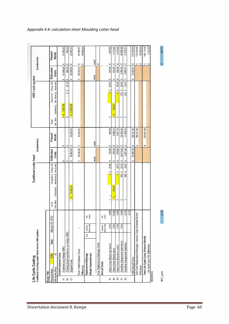
Dissertation document B. Kemps Page 60
Appendix 4.4: calculation sheet Moulding cutter head

Dissertation document B. Kemps Page 61
Appendix 4.5: Input parameters Coating line

Dissertation document B. Kemps Page 62
Appendix 4.6: Calculation sheet Coating line

Dissertation document B. Kemps Page 63
Appendix 4.7: Input parameters Double vacuum box

Dissertation document B. Kemps Page 64
Appendix 4.8: Calculation sheet Double vacuum box

Dissertation document B. Kemps Page 65
Appendix 5: Results
The first graph for each case reflects a simple but practical sensitivity analysis. “Reeks 1” simulates
the evolution in cost difference between the two alternatives, using the standard parameters. The
other curves, “Reeks 2”, ”Reeks 3”,”Reeks 4”, visualize the effect when some parameters are slightly
changed. The advantage of this type of graph is that it visualizes the total cost difference at each
moment in time for each series (“reeks”).
The second graph visualizes the probability distribution of the net present worth difference between
the two options. The distribution shows which alternative is likely to be most interesting. The more
the graph appears to be on the right side of the zero meridian, the more likely it will be that the
second alternative is most attractive. On the other hand when the graph turns out to be more
negative (more towards the left side of the zero meridian), it suggests that, from an economic point
of view, the first option will probably turn out to be the best choice.
The third graph for each case indicates the uncertainty of the different input parameters. This
uncertainty analysis indicates which input parameters have the highest uncertainty in the different
alternatives. The higher the correlation the more the uncertainty of the input parameter affects the
uncertainty of the net present worth difference. The best way to reduce the uncertainty of the net
present worth difference is to make a better estimate about the input parameters with the highest
correlation.
The fourth graph for each case is the result of the sensitivity analysis. It shows the propagation of the
uncertainty of the different input parameters. For this analysis the uncertainty of the input
parameters is always equal (10%). The output shows the propagation of this uncertainty of ten
percent in the end result. The input parameters with the highest correlation influence the result the
most. In other words, changing ten percent on the input parameters is most effective for those
parameters that have the highest correlation factor in the sensitivity analysis.

Dissertation document B. Kemps Page 66
Appendix 5.1: Weinig versus Leadermac
Graph 1: Simple sensitivity analysis over the years, case 1
Reeks 1 Reeks 2 Reeks 3 Reeks 4
Discount rate: 9% 7% 5% 9%
Escalation labour costs: 2% 2% 2% 3%
Escalation hardware costs: 3% 3% 3% 4%
Escalation energy costs: 4% 4% 4% 5%
Waarde daling Weinig: 10% 10% 10% 10%
Waarde daling Leadermac: 15% 15% 15% 15%
Purchase Weinig: € 320.000,00 € 320.000,00 € 320.000,00 € 320.000,00
Purchase Leadermac: € 192.000,00 € 192.000,00 € 192.000,00 € 192.000,00
Purchase new surface: € 15.000,00 € 15.000,00 € 15.000,00 € 15.000,00
Purchase new bearings: € 500,00 € 500,00 € 500,00 € 500,00
Purchase new axis: € 3.000,00 € 3.000,00 € 3.000,00 € 3.000,00
Update software: € 9.250,00 € 9.250,00 € 9.250,00 € 9.250,00
Standard labour costs (/hour): € 20,10 € 20,10 € 20,10 € 20,10
Overtime costs (/hour): € 28,70 € 28,70 € 28,70 € 28,70
Technical staff costs (/hour): € 25,00 € 25,00 € 25,00 € 25,00
Table 2: Significant input parameters related to graph 1
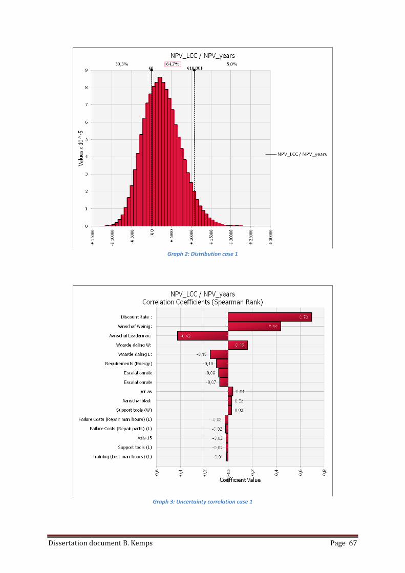
Dissertation document B. Kemps Page 67
Graph 2: Distribution case 1
Graph 3: Uncertainty correlation case 1

Dissertation document B. Kemps Page 68
Graph 4: sensitivity correlation case 1

Dissertation document B. Kemps Page 69
Appendix 5.2: Moulding cutter head
Graph 5: Simple sensitivity analysis over the years, case 2
Reeks 1 Reeks 2 Reeks 3 Reeks 4
Discount rate: 9% 9% 7% 9%
Escalation labour costs: 2% 2% 2% 3%
Escalation hardware costs: 3% 3% 3% 3%
Escalation energy costs: 4% 4% 4% 4%
Changeover time Traditional (min.) 15 16 15 15
Changeover time HSK system (min.) 10 9 10 10
Standard labour costs (/hour): € 20,10 € 20,10 € 20,10 € 20,10
Overtime costs (/hour): € 0,29 € 0,29 € 0,29 € 0,29
Technical staff costs (/hour): € 25,00 € 25,00 € 25,00 € 25,00
Table 3: Significant input parameters related to graph 5

Dissertation document B. Kemps Page 70
Graph 6: Distribution case 2
Graph 7: Uncertainty correlation case 2
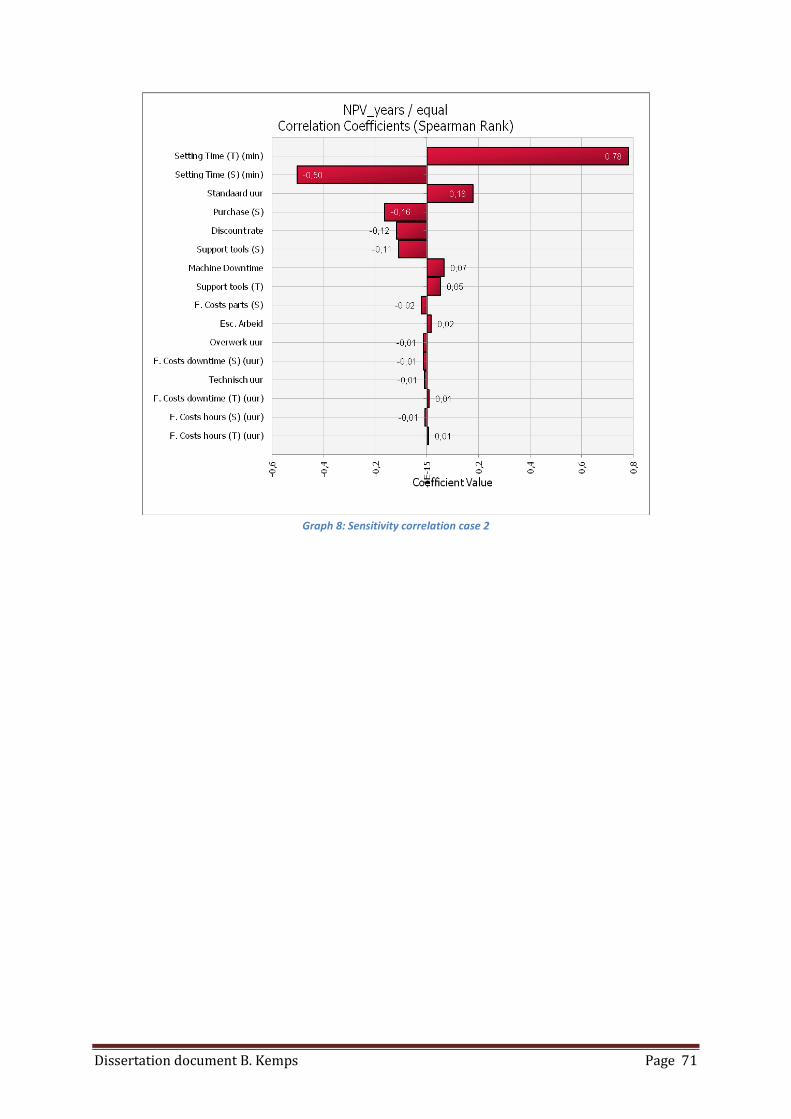
Dissertation document B. Kemps Page 71
Graph 8: Sensitivity correlation case 2

Dissertation document B. Kemps Page 72
Appendix 5.3: Coating line
Graph 9: Simple sensitivity analysis over the years, case 3
Reeks 1 Reeks 2 Reeks 3 Reeks 4
Discount rate: 9% 7% 9% 9%
Escalation labour costs: 2% 2% 2% 2%
Escalation hardware costs: 3% 3% 3% 3%
Escalation energy costs: 4% 4% 4% 4%
Value decrease soph. line: 10% 10% 10% 15%
Surcharge sophisticated line: € 265.000,00 € 265.000,00 € 265.000,00 € 265.000,00
Production a day (meters): 10.000 10.000 12.000 10.000
Standard labour costs (/hour): € 20,10 € 20,10 € 20,10 € 20,10
Overtime costs (/hour): € 0,29 € 0,29 € 0,29 € 0,29
Technical staff costs (/hour): € 25,00 € 25,00 € 25,00 € 25,00
Table 4: Significant input parameters related to graph 9

Dissertation document B. Kemps Page 73
Graph 10: Distribution case 3
Graph 11: Uncertainty correlation case 3

Dissertation document B. Kemps Page 74
Graph 12: sensitivity correlation case 3

Dissertation document B. Kemps Page 75
Appendix 5.4: Double vacuum box
Graph 13: Simple sensitivity analysis over the years, case 4
Reeks 1 Reeks 2 Reeks 3 Reeks 4
Discount rate: 9% 7% 9% 9%
Escalation labour costs: 2% 2% 4% 2%
Escalation hardware costs: 3% 3% 5% 3%
Escalation energy costs: 4% 4% 6% 4%
Surcharge double box: € 15.000,00 € 15.000,00 € 15.000,00 € 30.000,00
Standard labour costs (/hour): € 20,10 € 20,10 € 20,10 € 20,10
Overtime costs (/hour): € 0,29 € 0,29 € 0,29 € 0,29
Technical staff costs (/hour): € 25,00 € 25,00 € 25,00 € 25,00
Table 5: Significant parameters related to graph 13

Dissertation document B. Kemps Page 76
Graph 14: Distribution case 4
Graph 15: Uncertainty analysis case 4

Dissertation document B. Kemps Page 77
Graph 16: sensitivity correlation case 4

Dissertation document B. Kemps Page 78
Appendix 6: Veteka, the pilot study
Veteka was formed about 40 years ago. During these past 40 years it has become one of the leading
companies in supplying the Dutch construction market of houses with finished wooden mouldings.
Veteka notices that the expectations of constructors are continuously being raised. Thus, their
market is changing, the batch sizes are decreasing, the products are becoming more client specific
and clients expect the products to be totally finished, which implies an increase in the total value
added. Consequently, in order for Veteka to remain competitive and maintain its position in the
market, the future demands that the company should adapt its production facilities. A few years ago,
Veteka already started this process by purchasing more flexible production equipment. It became
clear that Veteka has little genuine expertise about the way the purchasing process takes place. Most
decisions are made based on experience and feelings.
At this moment there is no clear insight into the total costs of the individual installations over their
technical lifespan in the company. In order to make cost-effective, well-founded decisions about new
assets, it is essential to create transparency of all costs over an asset’s technical lifespan (within this
company).
To give some insight in our company, some essential characteristics will be given. Veteka currently
has two different production plants. In total, they own around 8 hectares of industrial ground
surface, of which a total of 2½ hectares have been built over. The total replacement value of all
installations directly contributing to the production process is calculated at between 9.500.000€ to
11.000.000€ (based on taxations in 2010). See also the table below.
Equipment Cost in € Number of
installations
Total value
in €
Internal transport (fork-lift –truck) 35.000 15 525.000
Air exhaust and heating installation 450.000 2 900.000
New “big” Lacquer installation 800.000 1 800.000
New small lacquer installation 150.000 3 450.000
Four sided moulder 450.000 4 1.800.000
Grinding equipment 300.000
Table 6: Essential characteristics of the replacement value of some used equipment
Related Documents