Lesson 5: ATM Networks, 1 st part Giovanni Giambene Queuing Theory and Telecommunications: Networks and Applications 2nd edition, Springer All rights reserved.

Lesson 5: ATM Networks, 1st partGiovanni Giambene

Queuing Theory and Telecommunications: Networks and Applications2nd edition, Springer

All rights reserved

Slide supporting material

© 2013 Queuing Theory and Telecommunications: Networks and Applications – All rights reserved


Introduction

ATM Introduction

Broadband ISDN (B-ISDN) was defined in 1990 by the ITU-T Recommendation I.150.

ATM is the name of a layer 2 protocol that characterizes the B-ISDN network.

The basic transmission unit is a packet of fixed length, named cell. The cell is composed of a payload of 48 bytes and a header of 5

bytes.

The cell header of 5 bytes contains all information to support the ATM protocol.

The payload of an ATM packet (cell) is transparently-managed by the network: there is no error control and flow control at intermediate nodes, but only end-to-end.

The transmission on the links uses a form of asynchronous time division multiplexing (i.e., no rigid slot assignment in the TDM frame).


ATM Introduction (cont’d) The ATM network is connection-oriented; switching is performed at layer 2.

Multimedia traffic classes can be managed by the ATM network. Each traffic class is described in terms of the bit-rate behavior and has guaranteed some Quality of Service (QoS) parameters (e.g., mean delay, packet loss rate, delay jitter, etc.).

Due to the connection-oriented nature of an ATM network, before a sender and a receiver can exchange data, an end-to-end path must be established by means of a set-up procedure.

During the set-up phase, an end-to-end path is established and it is verified [Connection Admission Control (CAC) protocol] that the resources on the links of the path are sufficient to support the new traffic guaranteeing for it (as well as for the already-active connections) the contractual QoS levels.


ATM Introduction (cont’d)

The ATM technology is quite expensive and not widely employed.

ATM is still a valid option for access networks, but not for backbone ones.

The ATM protocol (layer 2) is used for the broadband Internet access through the twisted-pair medium of the telephone network (Asynchronous Digital Subscriber Line, ADSL).

The ATM technology is also used for some geostationary satellite networks.


ATM: Multiplexer and Switch

An ATM network is typically formed of two different network elements: Switches

Multiplexers/demultiplexers (DSLAM).


ATM Multiplexer (DSLAM)

A multiplexer typically allows passing from low utilization input lines to high utilization output lines, i.e., a traffic concentrator that exploits the statistical multiplexing gain in the presence of bursty traffic sources.


M U X

Input TDM line #1

Input TDM line #2

Input TDM line #N

. . . . . . . Output TDM line

Each slot may contain an ATM cell

ATM Switch

A switch connects TDM input lines to TDM output lines. Each packet of a given input line must be analyzed by the processor of

the switch.

The virtual path description in the cell header permits to switch the packet on the appropriate output link on the basis of suitable switching tables.

Different switch technologies are available. In general, we can consider that, internally to the switch, there are buffers at input lines or at output lines.


Input TDM line #1

Input TDM line #2

Input TDM line #N

. . . . . . .

Each slot may contain an ATM cell

Output TDM line #1

Output TDM line #2

Output TDM line #N

. . . . . . .

SWITCH

= Switch symbol

ATM Network

Multiplexers and demultiplexers are used at the edge of the network. Switches are core elements.

There are two types of interfaces: The User-to-Network Interface (UNI): the interface for the access of

the user to the network.

The Network-to-Network Interface (NNI): the interface between to internal network elements.


Terminal B

Terminal C

UNI

UNI

Terminal A

UNI

Terminal D

UNI

ATM network

Virtual Path and Virtual Channel

The cell header contains the description of the virtual path characterized by means of two fields: Virtual Path Identifier (VPI) and Virtual Channel Identifier (VCI).

The physical transmission links employed by ATM are typically based on optical fibers (SDH).


Virtual path

Virtual channels

PHY Link

An ATM connection is characterized by the couple (VPI, VCI). These values may change at each switch.

Protocol Stack

ITU-T Recommendation I.321 characterizes the ATM protocol stack.

The ATM protocol stack is three-dimensional, with three planes: User plane, for the end-to-end transfer of information traffic;

Control plane, for signaling traffic needed to admit a new connection, for the maintenance of the connection and, finally, for the release of the connection;

Management plane, for operation and maintenance functions and for the coordination of the different planes.


Physical layer

ATM

Management plane

Pla

ne

man

agem

ent

Lay

er m

anag

emen

t

Control plane User plane

ATM Adaptation Layer (AAL)

Higher layer protocols Higher layer protocols Both user and control planes are characterized by two (stacked) protocols at layer 2: ATM Adaptation Layer (AAL) and the proper ATM layer.

ATM Cell

In previous data networks (i.e., X.25 and frame relay) the switched unit was a packet (or frame) of variable length.

In the ATM case, a fixed-length packet, called ‘cell’ (5-byte header and 48-byte payload), has been defined as a result of a complex standardization process that took different aspects into account, such as: Efficient utilization of transmission resources;

End-to-end delay to transfer a cell;

Routing / switching complexity;

Delay to cross a node.

A PDU received from higher layer protocols is fragmented into many ATM cells (the last cell is only partially used thus causing a loss of efficiency).


ATM Cell (cont’d)

The cell header reduces the transmission efficiency, since header bits do not carry information (H = number of bytes of the cell header; P = number of bytes of the cell payload). The efficiency of the cell can be expressed as:

On a link with a physical capacity of 155 Mbit/s, about 14.6 Mbit/s are lost due to the cell headers; this is a considerable capacity that has to be used to support the ATM protocol.

The use of a fixed-length packet permits to reduce the delays encountered at the queue for the transmission on a link. This is based on the comparison of the queue delay for M/M/1 and

M/D/1 queuing systems with same traffic intensity r.© 2013 Queuing Theory and Telecommunications: Networks and Applications – All rights

reserved

53

48

HP

P

Message Switching versus Cell Switching Let E[X] denote the mean packet/cell transmission duration.

In the ATM case X is constant.

The mean delay T experienced at a transmission buffer for the packet/cell transmissions (M/M/1 vs. M/D/1) can be expressed by means of the Pollaczek-Khinchin formula:

The use of cells of fixed-length (M/D/1 case) permits to reduce the queuing delays with respect to packets of variable length (M/M/1 case) with the same traffic intensity.


M/M/1for ,12

2

M/D/1for ,12

12 2

2

2

XE

XEXE

XE

XEXE

XE

XEXET

More details on this formula will be provided in Lesson No. 7.

ATM Cell Structure

The cell structure is defined in ITU-T Recommendation I.361.


GFC VPI

VCI

VPI VCI

VCI PT CLP

HEC

Payload

Cell format at UNI

VCI

VPI VCI

VCI PT CLP

HEC

Payload

Cell format at NNI

VPI

5-b

yte

hea

der

48

-byt

e p

aylo

ad

5-b

yte

hea

der

48

-byt

e p

aylo

ad

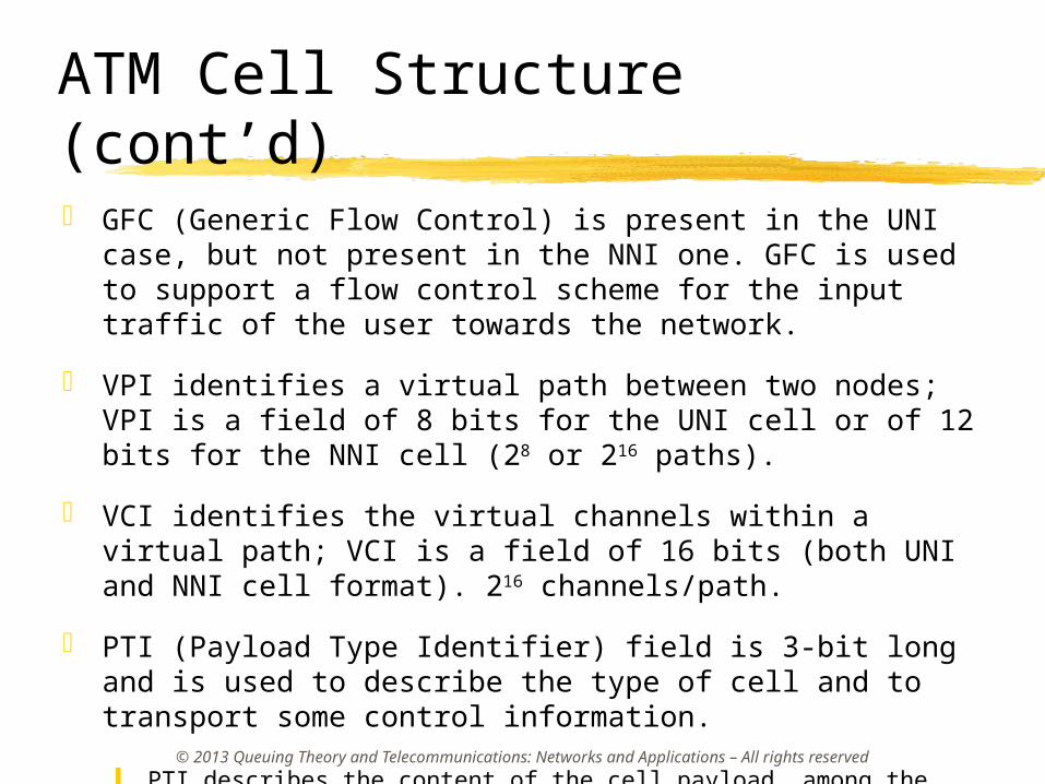
ATM Cell Structure (cont’d)

GFC (Generic Flow Control) is present in the UNI case, but not present in the NNI one. GFC is used to support a flow control scheme for the input traffic of the user towards the network.

VPI identifies a virtual path between two nodes; VPI is a field of 8 bits for the UNI cell or of 12 bits for the NNI cell (28 or 216 paths).

VCI identifies the virtual channels within a virtual path; VCI is a field of 16 bits (both UNI and NNI cell format). 216 channels/path.

PTI (Payload Type Identifier) field is 3-bit long and is used to describe the type of cell and to transport some control information. PTI describes the content of the cell payload, among the following

cases: information data, Operation, Administration, and Maintenance (OAM), Resource Management (RM) signaling.


ATM Cell Structure (cont’d)

CLP (Cell Loss Priority) bit denotes whether the cell has low (CLP = 1) or high (CLP = 0) priority.

Low priority cells can be dropped if switch queues are congested. CLP bit can be set either by the sender to differentiate the priority among different cells or by the access node in case that the connection violates its traffic contract with the network. The CLP bit has a similar role to the DE bit in the packet header of frame relay.

HEC (Header Error Control) field of one byte makes the parity check of just the cell header at each hop (the PHY layer on the basis of 32 bits of the cell header generates the last 8 parity bits of the same cell header).

Due to the high reliability of the transmission medium (optical fiber) it is not convenient to check the integrity of the entire cell (this task will be performed only end-to-end). Only the header is verified: if the cell header is correct (or with a single error that is corrected) the cell is further forwarded, otherwise the cell is discarded.

The HEC code is also used to find the appropriate cell synchronism in a received stream of ATM cells (SDH). The correlation in the header bits introduced by HEC is almost unique in the cell (it is unlikely that the same correlation on 40 bits is verified in another position of the cell). Such characteristic is important when the ATM traffic stream has to be extracted from complex physical layer multiplexed streams.



ATM Protocol Stack

ATM Protocol Stack

PHY layer is divided into two sub-layers: Physical Medium (PM) in charge of physical layer-related functions (electro-optic conversion of bits and bit timing) and Transmission Convergence (TC) that generates the cell HEC field.

ATM layer operates the following functions: Flow control at the UNI by means of the GFC;

Generation of the first 4 bytes of the ATM cell header;

Translation of the VPI&VCI fields from input to output of a switch;

Multiplexing (and demultiplexing) of the cells of different VPIs and VCIs on the same stream.

AAL layer is operated only end-to-end and not at intermediate ones. The AAL layer is sub-divided into two different sub-layers: Segmentation And Reassembly (SAR) and Convergence Sublayer (CS). AAL layer has the following tasks:

End-to-end transfer of messages of various lengths with cells of fixed length (segmentation/reassembly);

Management of erroneous cells and lost cells;

Flow control and congestion control;

Timing of the transported flow;

Multiplexing of different traffic flows on the same ATM connection.


ATM Protocol Stack (cont’d)

SAR functions are as follows:

In transmission, SAR divides the PDUs received from the CS sub-layer into smaller units (SAR-SDUs) that, with some added control, form the SAR-PDUs that fit with the cell payload length (segmentation); in reception, SAR re-obtains the PDU for the CS sub-layer.

SAR performs the Cyclic Redundancy Check (CRC) on the information bits.

SAR introduces bits in the payload of each cell that, depending on the AAL type, have a different function. For instance, cell numbering, PDU length in cells, etc.

CS function is to manage the higher layer PDUs for the different services supported, thus providing to SAR a CS PDU, including header and trailer control bits. © 2013 Queuing Theory and Telecommunications: Networks and Applications – All rights

reserved

CS

SAR

ATM

A A L

TC

PM

P H Y

Higher layers LL AA YY EE RR

MM AA NN GG..

ATM and ITU-T Traffic Classes

Traffic classes are differentiated on the basis of time criticality of the information transfer, bit-rate behavior, and type of connection. The ITU-T Recommendations of the I.363.x series describe the AAL characteristics for ITU-T traffic classes A, B, C, and D.

We will see later how these generic definitions of traffic classes have been implemented in ATM by means of ATM Adaptation Layers (AAL).


Class A Class B Class C Class D

Real-time traffic Non-real-time traffic

Constant bit-rate traffic Variable bit-rate traffic

Connection-oriented services Connection-less services

ATM Traffic Classes and AAL

AAL1 is used for Class A for the support of services with circuit emulation (dedicated end-to-end circuit). AAL1 is used for Constant Bit-Rate (CBR) real-time traffic for audio, video, and, in general, isochronous applications.

AAL2 is used for class B for real-time Variable Bit-Rate (rt-VBR) and for connection-oriented traffic. AAL2 can be used for voice and video packet services. AAL2 allows multiplexing of different AAL2 flows on the same ATM connection with given VPI and VCI fields by means of suitable flow identifiers.

AAL3 and AAL4 have practically the same characteristics. They can be used for Class C and Class D, that is non-real-time Variable Bit-Rate (nrt-VBR) traffic for connection-oriented (e.g., frame relay) or connection-less services. The AAL3/AAL4 protocol allows multiplexing of different flows on the same connection by means of suitable flow identifiers.

AAL5 has been conceived to simplify AAL3/AAL4; it is the most simple and efficient adaptation protocol for supporting services for all the different traffic classes except CBR. AAL5 does not support the multiplexing of different AAL flows.

All AAL levels introduce some degree of overhead explained as follows.© 2013 Queuing Theory and Telecommunications: Networks and Applications – All rights

reserved

ATM Traffic Classes and AAL (cont’d)


Class A (circuit

emulation)

Class B (packetized voice/video)

Class C (connection-

oriented data)

Class D (Datagram)

Type of AAL AAL1 AAL2AAL3 AAL4

AAL5

Timing between

source and destination

Real-timeNon-Real-Time

Bit-rate Constant VariableConnection

mode Connection-oriented Connection-less

AAL1 Example

The 48-byte cell payload format for AAL1:

The Sequence Number (SN) field is used for denoting lost cells;

The Sequence Number Protection (SNP) is a code used to protect the SN field.

The remaining 47 bytes form the effective cell payload with AAL1 and the fragmentation unit operated by the SAR sub-layer in this case.


SN SNP SAR-SDU

1 byte 47 bytes

4 bits 4 bits

AAL2 Example

The AAL2 internal protocol architecture entails: Service Specific Conversion Sublayer (SSCS),

Common Part Sublayer (CPS).

SSCS receives the higher layer PDU and formats a CPS packet (see next slide picture) to be included in the CPS PDU. Such PDU becomes the payload of the underlying ATM layer cell. The Channel IDentifier (CID) field is a logical identifier of the virtual

connection to which this information unit belongs.

The Length Indicator (LI) field denotes the length of the CPS packet; the default value considered here is 45 bytes so as to fit the CPS packet in just one CPS PDU that represents the cell payload with AAL2.

The User-to-User (UUI) field is used to convey end-to-end user data or to support OAM operations.

The Header Error Control (HEC) is a code to protect the first 19 bits of the CS PDU.


AAL2 Example (cont’d)

CS packet format:


CID LI

3 bytes

payload

45 bytes

8 bits 6 bits

UUI HEC

5 bits 5 bits

AAL5 Example

AAL5 uses a cumulative overhead at the CS PDU level: a 8-byte trailer is added. For simplicity, the CS PDU is made of a length multiple of 48 bytes (a

PAD field is used to adjust properly the length).

The CS PDU payload has a variable length up to 65535 bytes to support IP packets (RFC 1577); such length is coded by the Length (LEN) field in the trailer.

The CRC field is used for revealing errors on the entire CS PDU.


8 bytes (trailer)

payload

48 bytes

…. CRC

4 bytes

PAD

0 – 47 bytes

payload

48 bytes

payload

48 bytes

LEN

CS PDU

2 bytes

CPI

1 byte

UU

1 byte

SAR-PDU Header SAR-PDU Header Header

ATM cell

SAR-PDU

AUU bit = 1 in the PTI field

ATM cell last ATM cell

65535 bytes (CS PDU payload)


ATM Switches

ATM Switches Architectures

A switch operates at layer 2 (ATM layer) and realizes the virtual circuit switching by receiving a cell on an input port with a given VPI+VCI and by switching it (according to routing instructions defined in the path set-up phase) to an output port with, in general, a new VPI+VCI couple (so that cell HEC changes).

Two possible switch architectures can be considered:

ATM cross-connect: a cell changes only its VPI from input to output,

Typical ATM switch: a cell changes both VPI and VCI from input to output.


Cross-Connect Switch

The ATM cross-connect switch can be considered as a first and simplified implementation of an ATM switch since it can switch at most 4096 (= 212, VPI field contains 12 bits) input virtual circuits.

In the example below, VPI = 10 is switched to VPI = 40 and VPI = 20 is switched to VPI = 30.


VVVPPPIII 111000 VCI 20 VCI 15

VVVPPPIII 444000

VCI 20 VCI 15



Classical Switch

In the example below, the input VCI = 20, VPI = 10 is switched to the output VCI = 1, VPI = 30.



VVVPPPIII 333000

VCI 1 VCI 2

VVVPPPIII 222000

VCI 1 VCI 2

VVVPPPIII 444000

VCI 20 VCI 15

VVVCCCIII 222000

VVVCCCIII 111

VC switching

VP switching

Details on the Switch Architecture Three major factors have a large impact on the

implementation of the ATM switch architecture: The high speed at which the switch has to operate (from 150 Mbit/s). The statistical behavior of the ATM flows crossing the switch. Switching elements use routing tables (these tables are almost pre-

complied to minimize the switch complexity defined at call set-up).

Input and output ports are associated with (VPI, VCI) couples.


(VPI, VCI)IN of the input cell

. . . . . . .

. . . . . . .

SWITCH (VPI, VCI)OUT of the output cell

PATH

Input port and output port of the switch on the same path

Routing table with association of input port and (VPI,VCI) and output port and (VPI, VCI) for each path

Set-up phase

of the path

Input buffering uses a dedicated buffer on each input port. Buffers manage cells in a First-Input, First-Output (FIFO) basis. A cell at the top of an input buffer may be blocked due to repeated conflicts on the destined output port with cells from other buffers. Such cell blocks all the other cells in the same buffer even if they could be delivered without conflicts to their output lines (Head-Of-Line blocking, HOL).


Thank you!

[email protected]

Lesson No. 8 contains the second part of this Lesson.

Lesson 5: ATM Networks, 1 st part Giovanni Giambene Queuing Theory and Telecommunications: Networks and Applications 2nd edition, Springer All rights reserved.

Documents