Lesson 12: IP Layer and Routing Giovanni Giambene Queuing Theory and Telecommunications: Networks and Applications 2nd edition, Springer All rights reserved Slide supporting material © 2013 Queuing Theory and Telecommunications: Networks and Applications – All rights reserved

Lesson 12: IP Layer and Routing Giovanni Giambene Queuing Theory and Telecommunications: Networks and Applications 2nd edition, Springer All rights reserved.
Dec 14, 2015
Welcome message from author
This document is posted to help you gain knowledge. Please leave a comment to let me know what you think about it! Share it to your friends and learn new things together.
Transcript

Lesson 12: IP Layer and RoutingGiovanni Giambene
Queuing Theory and Telecommunications: Networks and Applications2nd edition, Springer
All rights reserved
Slide supporting material
© 2013 Queuing Theory and Telecommunications: Networks and Applications – All rights reserved

© 2013 Queuing Theory and Telecommunications: Networks and Applications – All rights reserved
IP Layer Introduction and IPv4

The Internet Protocol Stack The Internet protocol is described by four functional levels in the protocol architecture:
The network layer is the lowest layer of the TCP/IP protocol hierarchy. The protocols in this layer provide the means for the system to route data to other network devices.
Addressing and routing are the main functions of network layer.
© 2013 Queuing Theory and Telecommunications: Networks and Applications – All rights reserved
Link Network hardware
Application
Transport
Network
e.g., FTP, Telnet, SMTP, HTTP
TCP
IP
UDP ICMP
ARP
e.g., SNMP
Hourglass Model
© 2013 Queuing Theory and Telecommunications: Networks and Applications – All rights reserved
Twisted pair Coaxial cable Optical fiber Wireless link
IEEE 802.3 IEEE 802.11
IP
TCP UDP
SMTP POP/IMAP HTTP P2P RTP/RTCP
Thunderbird Silverlight Fire Fox VoIP/Skype/
GoogleTalk/MSN Media players (e.g., Polycom)
SIP
Waist of the Internet protocol hourglass model
SIP client
MAC layer protocols
Network layer protocols
Transport layer
protocols
Applications
Application layer
protocols
PHY layer
The Internet protocol stack has a layered architecture resembling an hourglass; on the waist of the hourglass there is just the IP protocol, the glue, the basis for everything.

IP Layer
Routing is the process to define routes among hosts from source to destination and to keep updated the routing tables.
Forwarding is the process executed at each router in order to find a suitable output port for an arriving packet on the basis of the routing table.
IP is an unreliable protocol because it does not perform error detection and recovery for the transmitted data. This does not mean that we cannot ‘rely’ on this protocol. IP can be relied upon to accurately deliver data to the destination network, but it does not check whether data are correctly received or not.
© 2013 Queuing Theory and Telecommunications: Networks and Applications – All rights reserved

IPv4 Addressing An IP address (IP version 4, IPv4) has a representation with 32 bits, written by considering the bits in groups of 8 and taking the corresponding decimal number. Each of these groups is written separated by a dot (i.e., dotted-decimal notation). Each number can range from 0 to 255.
The specification of IP addresses is contained in RFC 1166.
An IP address consists of a pair of numbers:
IP address = <network identifier> + <host identifier>
A router receiving an IP packet extracts the network address of the destination, which is classified by examining its first bits. Once the address class has been determined (see next slide), routers ignore host bits, and only need to look at the network bits to find a route.
© 2013 Queuing Theory and Telecommunications: Networks and Applications – All rights reserved

IPv4 Address Classes
For the above classes, the address of a network has all host bits equal to ‘0’. Whereas, the broadcast address of a network is characterized by all host bits equal to ‘1’.
© 2013 Queuing Theory and Telecommunications: Networks and Applications – All rights reserved
Class A 0 8 16 24 31
network host
Class B
network host
Class C
network host
Class D
multicast
Class E
reserved
0
10
110
1110
1111

IPv4 Address Classes (cont’d)
Class A: First bit set to ‘0’ plus 7 network bits; 24 host bits Initial byte ranging from 0 to 127 Totally, 128 (= 27) Class A network addresses are available (0 and 127 network
addresses are reserved) 16,777,214 (= 224-2) hosts can be addressed in each Class A network
Class B: First two bits set to ‘10’, plus 14 network bits; 16 host bits Initial byte ranging from 128 to 191 Totally, 16,384 (= 214) Class B network addresses 65,534 (= 216-2) hosts can be addressed in each Class B network
Class C: First three bits set to ‘110’ plus 21 network bits; 8 host bits Initial byte ranging from 192 to 223 Totally, 2,097,152 (= 221) Class C network addresses 254 (= 28-2) hosts can be addressed in each Class C network
© 2013 Queuing Theory and Telecommunications: Networks and Applications – All rights reserved

IPv4 Subnetting Due to the explosive growth of the Internet, there is a strong need for an efficient use of IP addresses. To avoid this problem, the concept of subnets has been introduced. In particular, the host number part of the IP address is further sub-divided into a sub-network number and a host number. The main network now consists of a number of sub-networks or subnets and the IP address is interpreted as:
<network number> + <subnet number> + <host number>
“Subnetting” is implemented in a way that is transparent to remote networks.
The organization of sub-networks within an IP network implies to use a subnet mask, i.e., a sort of ‘filter’ needed by the router to identify the sub-networks connected.
© 2013 Queuing Theory and Telecommunications: Networks and Applications – All rights reserved

IPv4 Subnetting (cont’d) Let us consider a router with many interconnected local networks, each forming a sub-network.
The mask is composed of a certain number of higher-order bits equal to ‘1’, while the remaining lower-order bits (corresponding to the host number) are equal to ‘0’.
When a packet arrives, the router makes the AND operation between the IP destination address of the packet and the available mask(s) to determine which sub-network the packet belongs to. Both the IP address and the mask(s) are in binary format. Such operation permits to extract both network and sub-network numbers from the IP address.
If the AND procedure yields a match with one of the sub-networks connected to the router, it forwards the packets through the appropriate interface towards the destination local network .
Otherwise, if the above match fails, the router has to send the packet towards the Internet (exterior network).
© 2013 Queuing Theory and Telecommunications: Networks and Applications – All rights reserved
Direct routing
Indirect routing

IPv4 Subnetting (cont’d)
When we speak about the default subnet mask for a given address class, we consider a mask that does not modify the length of the host part of the address. The following standard subnet masks can be used: 255.0.0.0 for class A 255.255.0.0 for class B 255.255.255.0 for class C.
Within a sub-network the host address with all bits equal to ‘0’ is used as sub-network address; whereas the host address with all bits equal to ‘1’ is used as sub-network broadcast address.
Example: given the class B network, 172.16.0.0, we can extend the network part of the address from 16 to 24 bits by selecting a subnet mask equal to 1111111111110000 (i.e., 255.255.255.0 in dotted-decimal notation). Now we can create for example two new sub-networks: 172.16.8.0 and 172.16.15.0, each one with up to 254 addressable hosts.
Referring to the above example, we could use the following notation for a host in the subnet 172.16.8.0: 172.16.8.1/24.
© 2013 Queuing Theory and Telecommunications: Networks and Applications – All rights reserved
IPv4 Packet Format
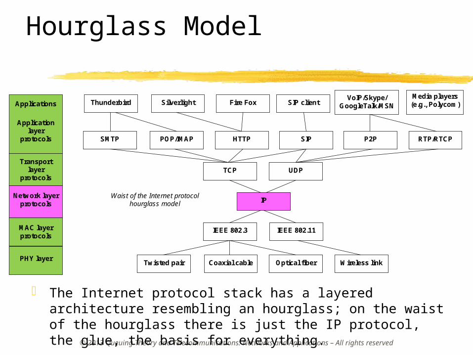
The IPv4 packet (datagram) format was defined in RFC 791. The IPv4 header carries some information that makes it rather large (minimum 20 bytes).
© 2013 Queuing Theory and Telecommunications: Networks and Applications – All rights reserved
Version H.length Type of Service Total Length
Identification Flags Fragment Offset
Time To Live Protocol Header Checksum
Source Address
Destination Address
Options
Padding
Data
Precedence Delay Throu-ghput
Reliabi-lity
Reserved
Reser-ved
DF MF
4 bits
32 bits 20
byt
es
Byte used for QoS support (IntServ or DiffServ)
Length of the whole IP packet, 16 bits

Some Fields of the IPv4 Packet Format TTL, Time To Live (8 bits): Specifies how long the datagram is
allowed to “live” in the network, in terms of router hops. Each router decreases by one the value of the TTL field prior to transmitting the related datagram. If the TTL field drops to zero, the datagram is not forwarded, but discarded, assuming that the datagram has taken a too long route.
Protocol (8 bits): Identifies the higher-layer protocol carried out in the datagram. This is used by the network layer to know to which transport layer process the packet has to be delivered. The values of this field were originally coded in IETF RFC 1700. For instance, the TCP protocol has a code equal to 6; the Internet Control Message Protocol (ICMP) protocol has a code equal to 1.
The maximum IP packet length is 65535 bytes.
© 2013 Queuing Theory and Telecommunications: Networks and Applications – All rights reserved

Some Fields of the IPv4 Packet Format (cont’d) Header Checksum (16 bits): A checksum computed over the
header to provide a basic protection against corruption. This is not the complex Cyclic Redundancy Check (CRC) code typically used by data link layer protocols. It is calculated by considering “the 16 bit one’s complement of the one’s complement sum of all 16 bit words in the header”. In particular, the 16 bit one’s complement sum is obtained by dividing the header in blocks of 16 bits (note that checksum bits are now considered to be equal to 0 in this case); these blocks are summed and the carry (if any) is summed to the result. Finally, the bits of the resulting binary number are complemented to obtain the checksum bits.
Since the TTL field changes at each hop, the checksum must be re-calculated at each hop. At each hop the device receiving the datagram performs the checksum verification and, in the presence of a mismatch, discards the datagram as damaged (otherwise the datagram could be misrouted).
© 2013 Queuing Theory and Telecommunications: Networks and Applications – All rights reserved

IPv4 Packet Size Distribution
In typical TCP/IP networks the IP packet size distribution is tri-modal: 40 byte packets (the minimum only-header TCP packet), 1500 byte packets (the maximum Ethernet payload size), and 552 / 576 byte packets (for TCP implementations that do not use Path Maximum Transmission Unit -MTU- Discovery, PMTUD).
The IP packet size distribution has been analyzed on the basis of the data acquired from the NASA Ames Internet Exchange (AIX) in 2000; data are available at the following link: http://www.caida.org/research/traffic-analysis/AIX/plen_hist/
A network analyzer software can be used to take traffic measurements and to characterize the packet size distribution. © 2013 Queuing Theory and Telecommunications: Networks and Applications – All rights
reserved

IPv4 Packet Size Distribution (cont’d) Internet traffic data
are studied by CAIDA (Cooperative Association for Internet Data Analysis). http://www.caida.org/
The graph shows the distribution of IP packet sizes at AIX.
The packet length distribution is generated from multiple short traces collected at various times of the day over two approximately one-week periods.
© 2013 Queuing Theory and Telecommunications: Networks and Applications – All rights reserved
40 564 15000
0.1
0.2
0.3
0.4
0.5
0.6
0.7
IP packet length
prob
abili
ty
This simplified distribution shows thatthe IP packet size distribution is tri-modal.

Introduction to Routing
Internet can be so large that one routing protocol cannot update the routing tables of all routers: it would be computationally unfeasible. Internet is divided into Autonomous Systems (ASs): An
AS is a group of networks and routers under the authority of a single administration.
An AS is also sometimes referred to as a routing domain or simply domain.
The routing problem is thus split into smaller (easier) sub-problems inside the ASs or between ASs. In particular, we have: Intra-domain routing: Routing inside an AS.
Inter-domain routing: Routing between ASs.© 2013 Queuing Theory and Telecommunications: Networks and Applications – All rights
reserved

Autonomous Systems
© 2013 Queuing Theory and Telecommunications: Networks and Applications – All rights reserved
AS #1
AS #2
AS #3
switch
router
inter-system interconnection

Hierarchical Structure of Domains A domain name is an identification label that defines a
realm of administrative autonomy, authority, or control in the Internet.
Domains are organized according to a hierarchical structure (sub-domains): The first-level of domains are the top-level domains, such
as .com, .net, .org, and the country code top-level domains. These domains are directly administered by the Internet Assigned Number Authority (IANA).
Below these top-level domains, there are second-level and third-level domains that represent (local area) networks needing to be interconnected to the Internet.
The registration of the domain names is usually administered by domain name Registries, which sell their services to the public.© 2013 Queuing Theory and Telecommunications: Networks and Applications – All rights
reserved

Hierarchical Structure of Domains (cont’d) Domain names are formed according to suitable rules and
procedures. IANA administers the data in the root nameservers, which form the top of the hierarchical Domain Name System (DNS) tree (http://www.iana.org/domains).
IANA delegates the management of local domains and blocks of IP addresses to Regional Internet Registries.
In Italy, the Registry of Italian Internet domains (.it), that is the national DNS, is provided by the Institute of Informatics and Telematics (IIT-CNR) in Pisa (http://www.nic.it/about-us/our-history-and-what-we-do).
At the request of ‘users’, the Registry associates a name with the long and difficult-to-memorize numerical IP address needed to navigate the Internet. This association is stored in an archive (the DNS) that all computers must query in order to reach a local domain.© 2013 Queuing Theory and Telecommunications: Networks and Applications – All rights
reserved

DNS
The DNS is basically a large distributed database, which resides on various computers and contains the associations of names and IP addresses of various routers and domains in the Internet.
The DNS has a hierarchical structure.
© 2013 Queuing Theory and Telecommunications: Networks and Applications – All rights reserved
root
.arpa
.edu
.gov
.mil .us
Partial DNS hierarchy with root and domains of different levels.
© 2013 Queuing Theory and Telecommunications: Networks and Applications – All rights reserved
Private/Public IP Addresses

Public IPv4 Addresses
So far we have considered IP addresses that are ‘public’: these numbers have the widest geographical validity. These public IP addresses are used for those servers that need to be reachable by the whole Internet: Web serves
E-mail servers (POP, SMTP protocols)
Database servers.
A local institution could purchase one or more IP sub-networks to interconnect to the Internet, but due to the limited number of public IP addresses that are available, this approach is very expensive.
© 2013 Queuing Theory and Telecommunications: Networks and Applications – All rights reserved

Private IPv4 Addresses
For realizing a local institution network (Intranet) there is no need to use public IP addresses. Internal IP addresses to the Intranet (i.e., ‘private’ IP addresses with local meaning) could be used with some translation functionality at the gateway of the local network towards the Internet.
Private IP addresses (RFC 1918) have not a global validity.
IANA has reserved the following three blocks of IP addresses for private networks: 10.0.0.0 - 10.255.255.255 (class A)
172.16.0.0 - 172.31.255.255 (class B)
192.168.0.0 - 192.168.255.255 (class C)© 2013 Queuing Theory and Telecommunications: Networks and Applications – All rights reserved
The first block is a single class A network number, while the second block is a set of 16 contiguous class B network numbers, and the third block is a set of 256 contiguous class C network numbers.

Network Address Translator (NAT) The NAT (RFC 1631 and 2663) permits to connect LANs with
private IP addresses to the Internet.
Advantages of using a NAT: Limits the number of public IP addresses to connect a LAN to the
Internet
The private addressing space is wide and this allows some flexibility and protection of local machines.
© 2013 Queuing Theory and Telecommunications: Networks and Applications – All rights reserved
One-t
o-m
any N
AT:
Loca
l ad
dre
sses
are
cla
ss
C o
nes
in t
his
exam
ple
.
Intranet
InternetPublic IP addresses
Private IP addresses
192.168.1.5
220.100.1.1192.168.1.1
192.168.1.2
192.168.1.3 192.168.1.4
Translation Modes
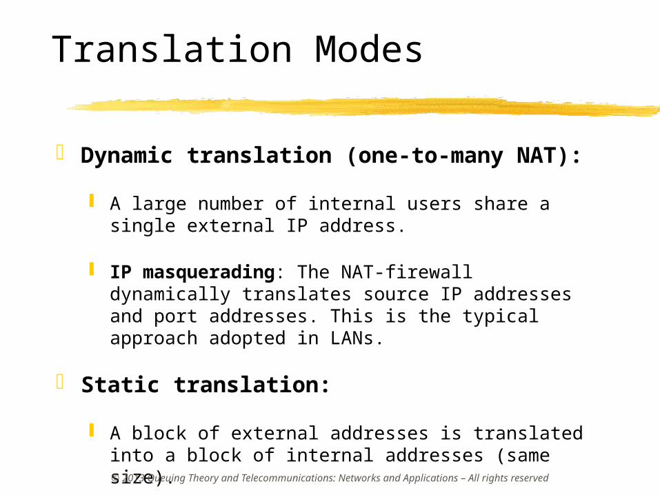
Dynamic translation (one-to-many NAT):
A large number of internal users share a single external IP address.
IP masquerading: The NAT-firewall dynamically translates source IP addresses and port addresses. This is the typical approach adopted in LANs.
Static translation:
A block of external addresses is translated into a block of internal addresses (same size).
© 2013 Queuing Theory and Telecommunications: Networks and Applications – All rights reserved

Example of a LAN with Details
© 2013 Queuing Theory and Telecommunications: Networks and Applications – All rights reserved
193.200.1.1 (Class C)
Switched Fast
Ethernet LAN @ 100
Mbit/s
Firewall (only some protocol
ports are open) with NAT and external DNS
10.0.0.1
Switch with layer3 - distribution
layer
Web Proxy server
(cache)10.0.0.2
Gateway/Router
LAN part withprivate IP addresses and VLANs
Switch of theaccess layer
Mask: 255.255.255.0
19
3.2
00
.1
.2
Internal DNS & DHCP server
10.0.0.3
'Alice' Web server &Email server10.0.0.4
Switch of theaccess layer
External link towardsthe Internet
LAN part withpublic IP addresses
DeMilitarized Zone (DMZ)
'Bob' Web serveroutside firewall-NAT
193.200.1.5
© 2013 Queuing Theory and Telecommunications: Networks and Applications – All rights reserved
Introduction to Routing

Direct and Indirect Routing
Direct routing occurs if the destination host is attached to a network to which the source host is also attached: an IP datagram can be sent directly, simply by encapsulating the IP datagram into the physical frame (MAC layer) of the network (LAN).
Instead, indirect routing occurs when the destination host is not in the same network of the source host: the only way to reach the destination is via one or more routers.
A host can recognize whether a route is direct or indirect by comparing the network and the subnet parts of source and destination addresses. If they match, the host may address the destination by using the Address Resolution Protocol (ARP). ARP is a protocol that dynamically associates a network-layer IP
address to a link-layer physical hardware address (i.e., MAC address).
For indirect routing, routing tables are used; these tables (generated/updated by routing protocols) provide the next hop (i.e., router) where to forward the IP packet for each network destination.© 2013 Queuing Theory and Telecommunications: Networks and Applications – All rights
reserved

Centralized and Distributed Routing
Centralized routing: the routing algorithm is run once for the whole network at the Routing Control Center (RCC), thus generating the different routing tables.
Decentralized routing: the algorithm is running in parallel at the different network nodes and converges to the definition of each routing table.
© 2013 Queuing Theory and Telecommunications: Networks and Applications – All rights reserved
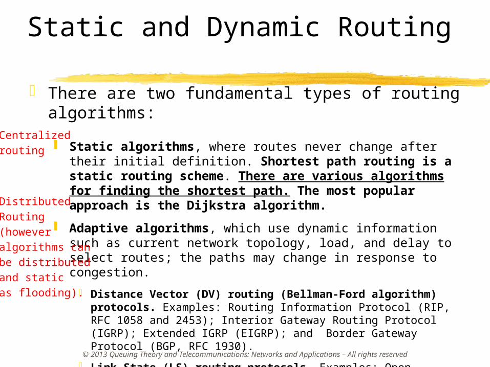
Static and Dynamic Routing
There are two fundamental types of routing algorithms: Static algorithms, where routes never change after their
initial definition. Shortest path routing is a static routing scheme. There are various algorithms for finding the shortest path. The most popular approach is the Dijkstra algorithm.
Adaptive algorithms, which use dynamic information such as current network topology, load, and delay to select routes; the paths may change in response to congestion.
Distance Vector (DV) routing (Bellman-Ford algorithm) protocols. Examples: Routing Information Protocol (RIP, RFC 1058 and 2453); Interior Gateway Routing Protocol (IGRP); Extended IGRP (EIGRP); and Border Gateway Protocol (BGP, RFC 1930).
Link State (LS) routing protocols. Examples: Open Shortest Path First Protocol (OSPF, RFC 2328 IPv4 and RFC 5340 IPv6) that uses the Dijkstra’s algorithm on a local image of the network topology; and Intermediate System to Intermediate System protocol (IS-IS, RFC 1142).
© 2013 Queuing Theory and Telecommunications: Networks and Applications – All rights reserved
Centralized routing
Distributed Routing(however algorithms can be distributed and staticas flooding).
Desirable Properties of Routing
Correctness
Simplicity
Robustness
Stability (the routing algorithm has converging routing tables)
Fairness
Optimality (minimizing mean packet delay vs. maximizing throughput)
© 2013 Queuing Theory and Telecommunications: Networks and Applications – All rights reserved
A. S. Tanenbaum. Computer Networks. Pearson Education, 2003.

General Comparisons of Routing Approaches
© 2013 Queuing Theory and Telecommunications: Networks and Applications – All rights reserved
The distributed routing algorithm could not converge (instability): routes can oscillate. BGP suffers from route oscillations.
Routing technique
Pros Cons
Static Simple and fast Not flexible
Dynamic Adapts to network changes Complex
CentralizedOne node performs
the routing algorithm
Vulnerability to failure of the node performing routing
functions
Decentralized Robustness to link failures
Routing convergence issues
and oscillations

Routed Routing Protocol
A routing protocol sends and receives signaling packets containing routing information to and from other routers.
In some cases, routing protocols can themselves run over routed protocols. Even if a routing protocol runs over a particular transport mechanism of layer (N), this does not mean that the routing protocol is of layer (N+1). OSPF, IGRP, and EIGRP run directly over IP; OSPF and EIGRP
have their own reliable transmission mechanisms, while IGRP uses an unreliable transport protocol.
RIP runs over UDP over IP
BGP runs over TCP over IP.© 2013 Queuing Theory and Telecommunications: Networks and Applications – All rights reserved

Shortest Path Algorithms
There are many shortest path algorithms. The most important shortest path algorithms are:
Dijkstra algorithm (good computational costs)
Bellman–Ford algorithm (good computational costs)
A* search algorithm
Floyd–Warshall algorithm
Johnson algorithm
Perturbation theory
© 2013 Queuing Theory and Telecommunications: Networks and Applications – All rights reserved
B. V. Cherkassky, A. V. Goldberg, T. Radzik, "Shortest Paths Algorithms: Theory and Experimental Evaluation", Mathematical Programming, Ser. A, Vol. 2, pp. 129-174, 1993.

Bellman Optimality Principle
The network is considered like an oriented graph with nodes (= routers) and edges (= links between routers).
If router j is on the optimal path from router i to k, then, also the optimal path from j to k is on the same path:
A consequence is that the set of optimal paths from a tagged router to all the routers form a tree, named sink tree for the tagged router.
This principle is adopted by the Dijkstra algorithm for shortest path routing.
© 2013 Queuing Theory and Telecommunications: Networks and Applications – All rights reserved
ik
j

Sink Tree
In the network, a sink tree of a node is a tree that connects this node to all other nodes of the network with the shortest path.
The sink tree (minimum spanning tree) of a node can be easily converted into the routing table of that node (i.e., a table showing the next hop for each destination to be reached from that node). A sink tree can be determined for each node of the network.
The picture below shows a network with all possible links (left) and the related sink tree for node B (right).
© 2013 Queuing Theory and Telecommunications: Networks and Applications – All rights reserved
D
B
C
EF
G
A
H
B
C
EF
G
A
H
© 2013 Queuing Theory and Telecommunications: Networks and Applications – All rights reserved
Dijkstra Routing Algorithm

Dijkstra Algorithm
The input is represented by the weight (= distance) of each link connecting nodes in the network. A weight equal to infinity means that there is no link between the two nodes.
The weight of a path (involving different routers in the network) is calculated as the sum of the weights of the edges (i.e., hops) in the path. A path from x to y is the ‘shortest’ one if there is no other path connecting x and y with a lower weight. If the weight is 1 for each link, the routing metric is hop count (related to the TTL field in IP packet header).
The Dijkstra algorithm finds the shortest path (i.e., the path with the lowest total weight) from x to y for increasing distance from x.
The Dijkstra algorithm is used to determine the sink tree for each node. The algorithm is repeated for all the nodes.
© 2013 Queuing Theory and Telecommunications: Networks and Applications – All rights reserved
E. W. Dijkstra, "A Note on Two Problems in Connexion with Graphs“, Numerische Mathematik, Vol. 1, pp. 269–271, 1959.

Dijkstra Algorithm (cont’d)
1. Let us start from the generic node A as source and we label all the other nodes of the graph with infinite costs.
2. We examine the nodes linked to node A and we re-label them with link numbers and link costs to A.
3. We create an extension of the path: we select the node to be added to the tree in the graph, which has the smallest cost and consider it as part of the shortest path tree for node A. If there are more possibilities with the same cost, we select the link with the lowest number. Let C denote the node selected and added to the tree at this step.
4. We re-label the nodes: the nodes that can be re-labeled are those not yet added to the shortest path tree, but linked to node C. Let B denote a generic node belonging to this set for potential re-labeling. The new label of B is formed of the number of the link connecting B to C and a new cost given by the sum of the B-C link cost with the cost in the label of C. The new label will actually substitute the old one if and only if the cost of the new label is lower than that of the old label (it can also happen that there are no label changes at a given step).
5. We go back to step #3, until all nodes of the graph are added to the shortest path tree of A.
© 2013 Queuing Theory and Telecommunications: Networks and Applications – All rights reserved

Dijkstra Algorithm (cont’d)
Dijkstra is a static and centralized algorithm, which allows to compute the routing tables for all the nodes of a network.
The Dijkstra algorithm completes a sink tree in a maximum number of iterations equal to n-1, where n is the number of network nodes. Therefore, the computational complexity of the Dijkstra algorithm for a network of n nodes is O(n2).
Note that there is a certain degree of redundancy in the sink trees of the different nodes. Hence, there is probably no need to completely recompute the sink trees for all nodes in the network; some tree parts can be reused on the basis of the optimality principle.
© 2013 Queuing Theory and Telecommunications: Networks and Applications – All rights reserved
Dijkstra Algorithm: An Example
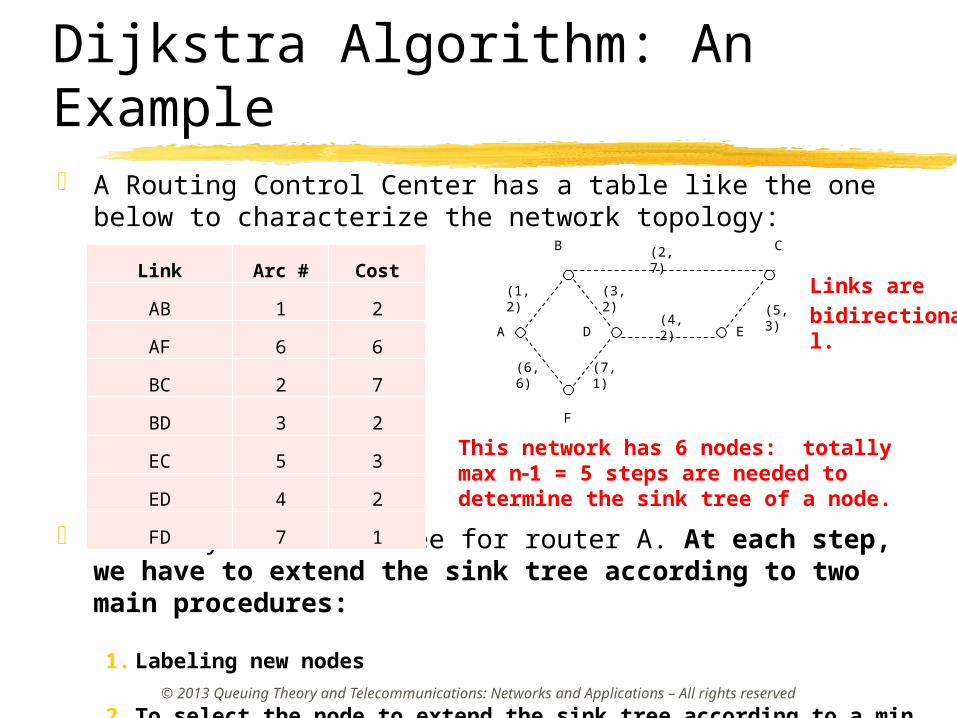
A Routing Control Center has a table like the one below to characterize the network topology:
We study the sink tree for router A. At each step, we have to extend the sink tree according to two main procedures: 1. Labeling new nodes
2. To select the node to extend the sink tree according to a min cost rule.
© 2013 Queuing Theory and Telecommunications: Networks and Applications – All rights reserved
(2,7)
(4,2)(5,3)
(1,2) (3,2)
(6,6) (7,1)
A
F
B C
ED
Link Arc # Cost
AB 1 2
AF 6 6
BC 2 7
BD 3 2
EC 5 3
ED 4 2
FD 7 1
This network has 6 nodes: totally max n-1 = 5 steps are needed to determine the sink tree of a node.
Links are bidirectional.

Dijkstra Algorithm: An Example (cont’d) We examine the nodes linked to A, which are labeled with the arc number
and the related costs (nodes not connected to A have a label with infinite cost)
We select node B because this is the node of the graph with the lowest cost in the label (= 2) and we consider arc #1 as part of the shortest path (sink tree) from node A.
A
F(6,6)
B(1,2) C(-,)
E(-,)
D(-,)
A
F(6,6)
B(1,2) C(-,)
E(-,)
D(-,)
1st STEP
© 2013 Queuing Theory and Telecommunications: Networks and Applications – All rights reserved

Dijkstra Algorithm: An Example (cont’d)
© 2013 Queuing Theory and Telecommunications: Networks and Applications – All rights reserved
A
F(6,6)
B(1,2) C(2,7+2)
E(-,)
D(3,2+2)
A
F(6,6)
B(1,2) C(2,9)
E(-,)
D(3,4)
2nd STEP
The new labels of nodes C and D now contain the total cost from the source node A: sum of the cost to B and the costs of the related arcs.
We examine the nodes linked to node B and not yet selected (i.e., nodes C and D): these nodes are re-labeled.
We select node D because this is the node of the graph having the lowest cost in the label (= 4) and we consider arc #3 as part of the shortest path (sink tree) from node A.

A
F(7,5)
B(1,2) C(2,9)
E(4,6)
D(3,4)
Dijkstra Algorithm: An Example (cont’d) We examine the nodes linked to node D and not yet selected (i.e., nodes E
and F): these nodes are re-labeled because both E and F have labels with higher costs ( and 6, respectively):
We select node F, because this is the node of the graph having the lowest cost in the label (= 5) and we consider arc #7 as part of the shortest path (sink tree) from node A.
© 2013 Queuing Theory and Telecommunications: Networks and Applications – All rights reserved
A
F(7,1+4)
B(1,2) C(2,9)
E(4,2+4)
D(3,4)
The new labels of nodes E and F now contain the total cost from the source node A.
3rd STEP

Dijkstra Algorithm: An Example (cont’d) There are not nodes not selected linked to F and hence labels do not need
to be updated. We thus move to the next phase.
We select node E, because this is the node of the graph having the lowest cost in the label (6<9) and we consider arc #4 as part of the shortest path (sink tree) from node A.
A
F(7,5)
B(1,2) C(2,9)
E(4,6)
D(3,4)
A
F(7,5)
B(1,2) C(2,9)
E(4,6)
D(3,4)
4th STEP
© 2013 Queuing Theory and Telecommunications: Networks and Applications – All rights reserved

Dijkstra Algorithm: An Example (cont’d)
A
F(7,5)
B(1,2) C(2,9)
E(4,6)
D(3,4)
A
F(7,5)
B(1,2) C(2,9)
E(4,6)
D(3,4)
At this point, the Dijkstra algorithm is completed: the shortest path (sink tree) for node A has been determined.
Arc #5 with cost 3
5th STEP
© 2013 Queuing Theory and Telecommunications: Networks and Applications – All rights reserved
We examine node C, the sole node linked to E and not yet selected. Its label does not change, because at a parity of cost (in this case 9 6+3), we select the label with the lowest arc number (2 5).
We select node C, because this is the sole node not yet selected and we consider arc #2 as part of the shortest path (sink tree) from node A.
Dijkstra Algorithm: An Example (cont’d)
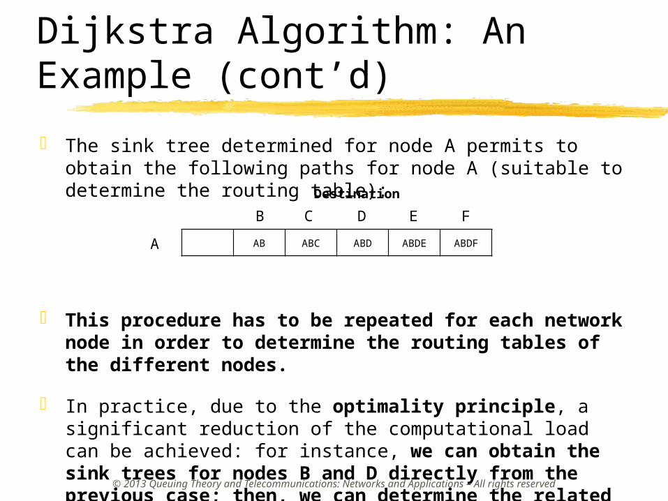
The sink tree determined for node A permits to obtain the following paths for node A (suitable to determine the routing table):
This procedure has to be repeated for each network node in order to determine the routing tables of the different nodes.
In practice, due to the optimality principle, a significant reduction of the computational load can be achieved: for instance, we can obtain the sink trees for nodes B and D directly from the previous case; then, we can determine the related routing table.
© 2013 Queuing Theory and Telecommunications: Networks and Applications – All rights reserved
AB ABC ABD ABDE ABDF
B C D E F
Destination
A

Dijkstra Algorithm: An Example (cont’d)
© 2013 Queuing Theory and Telecommunications: Networks and Applications – All rights reserved
The centralized routing algorithm permits to achieve the following paths for the different nodes :
The routing table is obtained considering for each destination just the next hop. For instance for a packet at node A and destined to node F, the routing table of node A has to provide the next hop B.
Destination
S
ou
rce

Dijkstra Algorithm: An Example (cont’d)
The central controller of the routing protocol computes the routing tables of the nodes and sends them to the nodes.
© 2013 Queuing Theory and Telecommunications: Networks and Applications – All rights reserved
Router A
Destination Arc
B 1
C 1
D 1
E 1
F 1
Router B
Destination Arc
A 1
C 2
D 3
E 3
F 3
Router C
Destination Arc
A 2
B 2
D 5
E 5
F 5
Router D
Destination Arc
A 3
B 3
C 4
E 4
F 7
Router E
Destination Arc
A 4
B 4
C 5
D 4
F 4
Router F
Destination Arc
A 7
B 7
C 7
D 7
E 7

© 2013 Queuing Theory and Telecommunications: Networks and Applications – All rights reserved
Flooding

Flooding Technique for Routing
Flooding entails that a router sends each arriving packet on every output link except the link from which the packet has arrived.
Flooding is a distributed and static routing scheme.
It is a quite simple routing scheme to be implemented and with limited processing requirements at the router: this routing scheme does not use routing tables.
Flooding can be used as a benchmark for other routing algorithms. Flooding always uses the shortest path, because it uses any possible path in parallel; as a consequence, no other protocol can achieve lower delays.
Flooding has practical applications in ad hoc wireless networks and sensor networks, where all the messages sent by a station can be received by all other stations in the transmission range.
Flooding is also used to update routing information with the link-state routing algorithm described later.
© 2013 Queuing Theory and Telecommunications: Networks and Applications – All rights reserved

Flooding Technique for Routing (cont’d) The problem with flooding is that it makes use of network
resources in a redundant way by involving a number of links, which increases as long as we move away from the source (initial) node, thus having the risk to cause congestion: flooding has the drawback to generate theoretically an infinite number of packets.
There are some techniques to limit the traffic generated:
A counter in each packet is decremented at each hop: when the counter reaches the 0 value, the packet is discarded.
Source router ID and sequence number is used in each packet: when a node receives the same packet a second time, the packet is discarded.
Selective flooding: packets are duplicated on the output links of the router only for those links that go in the right direction; suitable routing tables are needed in this case.© 2013 Queuing Theory and Telecommunications: Networks and Applications – All rights
reserved
© 2013 Queuing Theory and Telecommunications: Networks and Applications – All rights reserved
Distance Vector Routing

Distance Vector Routing
The Distance Vector routing protocol is a distributed and iterative scheme, based on the Bellman-Ford algorithm.
ss
Each router in the network sends on all links (interfaces) the list of destinations that it can reach and their distances from it (this is the distance vector).
In the vector, the destination is represented by an IP address and the distance is represented by the minimum cost to reach it.
The Distance Vector algorithm at the first round only contains the distances with adjacent connected routers (1 hop) and increases the number of hops covered at each iteration until the network diameter is reached.
Each router receives from its neighbor the list of destinations with the related distances. Then, the distance vector is stored after having summed the distances advertised by its neighbor node with the distance from the neighbor node.
The routing table is obtained by means of a fusion of distance vectors received from all neighbor nodes according to the following method: the interface to be selected to forward a packet towards a destination is that with the minimum resulting distance for that destination.
© 2013 Queuing Theory and Telecommunications: Networks and Applications – All rights reserved

Distance Vector Routing (cont’d) With the Distance Vector algorithm, each router starts
with a set of routes for those networks or sub-networks to which it is directly attached. This list is kept in a routing table, where each entry identifies a destination network or host and gives the ‘distance’ to that network.
Distance Vector uses the hop count metric, which does not take link speed (bandwidth), delay, and reliability into account. The distance vector could be extended to contain not only a distance for each destination, but also a direction in terms of the next-hop router
Distance vector updates are sent to adjacent routers on a periodical basis, ranging from 10 s to 90 s. When a report arrives at router B from router A, B examines the set of destinations it receives and the distance to each of them. B will update its routing table if: A knows a shorter way to reach a destination.
A provides a destination that B has not in its table.
The distance of A to a destination, already routed by B through A, has changed.
© 2013 Queuing Theory and Telecommunications: Networks and Applications – All rights reserved

Distance Vector Routing (cont’d)
© 2013 Queuing Theory and Telecommunications: Networks and Applications – All rights reserved
Let us examine how router R3 updates its routing table using the distance vectors (providing the cost to reach different IP networks) received from neighbor routers R1, R2, and R4. For instance we consider the routing towards the IP network 12.0.0.0. Router R3 receives the cost (distance) 4 from router R1 and sums the link cost R3-R1, which is equal to 5; hence, the total cost to reach 12.0.0.0 from router R3 through router R1 is 4+5 = 9. Analogously, R3 knows that the total cost to reach 12.0.0.0 through router R2 is 0+15 = 15. Finally, R3 knows that the total cost to reach 12.0.0.0 through router R4 is 15+5 = 20.Hence, router R3 updates its routing table selecting the path through router R1 to reach 12.0.0.0 with cost 9. Router R3 updates analogously its routing table for all destination networks received from adjacent routers. The routing table thus obtained contains the distance vectors that R3 will send to all its neighbors at the next iteration.
link cost = 5
link cost = 5
link cost = 15
R1
R2
R3
R4
Distance Vector sent by R1
Distance Vector sent by R2
Distance Vector sent by R4
Routing table generated at R3 by merging the distance vectors and selecting the lowest cost for
each destination
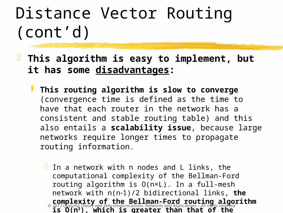
Distance Vector Routing (cont’d) This algorithm is easy to implement, but it
has some disadvantages: This routing algorithm is slow to converge
(convergence time is defined as the time to have that each router in the network has a consistent and stable routing table) and this also entails a scalability issue, because large networks require longer times to propagate routing information.
In a network with n nodes and L links, the computational complexity of the Bellman-Ford routing algorithm is O(n×L). In a full-mesh network with n(n-1)/2 bidirectional links, the complexity of the Bellman-Ford routing algorithm is O(n3), which is greater than that of the Dijkstra algorithm, given by O(n2).
© 2013 Queuing Theory and Telecommunications: Networks and Applications – All rights reserved

Distance Vector Routing (cont’d)
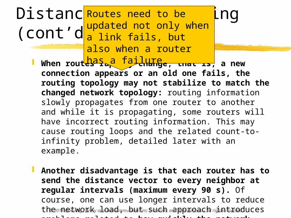
When routes rapidly change, that is, a new connection appears or an old one fails, the routing topology may not stabilize to match the changed network topology: routing information slowly propagates from one router to another and while it is propagating, some routers will have incorrect routing information. This may cause routing loops and the related count-to-infinity problem, detailed later with an example.
Another disadvantage is that each router has to send the distance vector to every neighbor at regular intervals (maximum every 90 s). Of course, one can use longer intervals to reduce the network load, but such approach introduces problems related to how quickly the network responds to changes in topology.
© 2013 Queuing Theory and Telecommunications: Networks and Applications – All rights reserved
Distance Vector Routing (cont’d)
When routes rapidly change, that is, a new connection appears or an old one fails, the routing topology may not stabilize to match the changed network topology: routing information slowly propagates from one router to another and while it is propagating, some routers will have incorrect routing information. This may cause routing loops and the related count-to-infinity problem, detailed later with an example.
Another disadvantage is that each router has to send the distance vector to every neighbor at regular intervals (maximum every 90 s). Of course, one can use longer intervals to reduce the network load, but such approach introduces problems related to how quickly the network responds to changes in topology.
© 2013 Queuing Theory and Telecommunications: Networks and Applications – All rights reserved
Routes need to be updated not only when a link fails, but also when a router has a failure.

Count-to-Infinity Problem
We have three routers in a linear topology: A connected to B and B connected to C.
We assume that the metric is computed in terms of hops, so that the cost of each link is ‘1’.
B calculates its distance to C as 1. A calculates its distance to C as 2.
We refer here to the basic version of the Distance Vector algorithm, where the distance vectors contain only the distances to the routers.
© 2013 Queuing Theory and Telecommunications: Networks and Applications – All rights reserved
A B C
B C
A 1 2
B A
C 1 2
A C
B 1 1
Distance vectors at the different
nodes at regime

Count-to-Infinity Problem (cont’d)
© 2013 Queuing Theory and Telecommunications: Networks and Applications – All rights reserved
A B C
A B C
B C
A 1 2
B A
C 1 2
A C
B 1 1
Distance vectors atthe different nodes
at regime
B C
A 1 2
A C
B 1 -
A B C
B C
A 1 2
A C
B 1 3
Link failure event
A B C
B C
A 1 4
A C
B 1 3
tim
e

Count-to-Infinity Problem (cont’d)
© 2013 Queuing Theory and Telecommunications: Networks and Applications – All rights reserved
Note
th
at
not
all
the lin
k
failu
res
lead t
o c
ount-
to-
infin
ity p
rob
lem
s.
A B C
We envisage that the link between B and C breaks. B realizes that it has to route through A the traffic destined to C. B recalculates its distance from C. B decides that it is now 3 hops away from C on the basis of the distance vector received from A, which contains the (old) distance 2 from C and also knowing that A is at a distance 1 from B. Since B has changed its distance vector, it sends this info to its remaining neighbors (i.e., A). Upon receiving a modified distance vector from B, A recalculates its distance vector and concludes that C is now 4 hops away (i.e., 3 hops away from B who is 1 hop away from A). A and B continue this process bouncing distance vectors so that their distances to C tend to infinity. At the end, they conclude that the best route to C is through the other node: packets to C are bounced between A and B until they are dropped (TTL = 0).
A B C
B C
A 1 2
B A
C 1 2
A C
B 1 1
B C
A 1 2
A C
B 1 -
A B C
B C
A 1 2
A C
B 1 3
A B C
B C
A 1 4
A C
B 1 3
B does not know that A routes the traffic through B itself to reach C. Hence, B takes a wrong decision here.
tim
e

Count-to-Infinity Problem (cont’d)
© 2013 Queuing Theory and Telecommunications: Networks and Applications – All rights reserved
Note
th
at
not
all
the lin
k
failu
res
lead t
o c
ount-
to-
infin
ity p
rob
lem
s.
A B C
We envisage that the link between B and C breaks. B realizes that it has to route through A the traffic destined to C. B recalculates its distance from C. B decides that it is now 3 hops away from C on the basis of the distance vector received from A, which contains the (old) distance 2 from C and also knowing that A is at a distance 1 from B. Since B has changed its distance vector, it sends this info to its remaining neighbors (i.e., A). Upon receiving a modified distance vector from B, A recalculates its distance vector and concludes that C is now 4 hops away (i.e., 3 hops away from B who is 1 hop away from A). A and B continue this process bouncing distance vectors so that their distances to C tend to infinity. At the end, they conclude that the best route to C is through the other node: packets to C are bounced between A and B until they are dropped (TTL = 0).
A B C
B C
A 1 2
B A
C 1 2
A C
B 1 1
B C
A 1 2
A C
B 1 -
A B C
B C
A 1 2
A C
B 1 3
A B C
B C
A 1 4
A C
B 1 3
A knows from its routing table that it routes through B to reach C and then if the cost from B to C has changed, A has to update its distance to C as well.
tim
e

Count-to-Infinity Problem (cont’d)
© 2013 Queuing Theory and Telecommunications: Networks and Applications – All rights reserved
Note
th
at
not
all
the lin
k
failu
res
lead t
o c
ount-
to-
infin
ity p
rob
lem
s.
A B C
We envisage that the link between B and C breaks. B realizes that it has to route through A the traffic destined to C. B recalculates its distance from C. B decides that it is now 3 hops away from C on the basis of the distance vector received from A, which contains the (old) distance 2 from C and also knowing that A is at a distance 1 from B. Since B has changed its distance vector, it sends this info to its remaining neighbors (i.e., A). Upon receiving a modified distance vector from B, A recalculates its distance vector and concludes that C is now 4 hops away (i.e., 3 hops away from B who is 1 hop away from A). A and B continue this process bouncing distance vectors so that their distances to C tend to infinity. At the end, they conclude that the best route to C is through the other node: packets to C are bounced between A and B until they are dropped (TTL = 0).
A B C
B C
A 1 2
B A
C 1 2
A C
B 1 1
B C
A 1 2
A C
B 1 -
A B C
B C
A 1 2
A C
B 1 3
A B C
B C
A 1 4
A C
B 1 3
tim
e

The RIP Protocol
The RIP protocol (defined in RFC 1058 and RFC 2453) is an intra-domain routing scheme based on the Distance Vector approach; it adopts the hop count as a cost metric.
The RIP protocol envisages a maximum number of hops equal to 15 in order to reach a destination; this permits to avoid routing loops, but limits the size of the network where RIP can be adopted.
RIP sends periodic route updates every 30 s; however, route updates can also be triggered by some changes in the network.© 2013 Queuing Theory and Telecommunications: Networks and Applications – All rights
reserved
The RIP Protocol (cont’d)
The following approaches permits to solve in part the count-to-infinity problem in Distance Vector routing.
Split-horizon routing: a router does not advertise the cost of a destination to a neighbor if this neighbor is the next hop towards that destination.
Split-horizon routing with poisoned reverse: each router includes in its messages towards an adjacent router the paths learned from that router, but using a metric (distance) equal to 16 (equivalent to infinity). This scheme is adopted by RIP.
© 2013 Queuing Theory and Telecommunications: Networks and Applications – All rights reserved

© 2013 Queuing Theory and Telecommunications: Networks and Applications – All rights reserved
Link State Routing
Link State Routing
Distance Vector Routing was used in ARPANET until 1979. The growth of the Internet pushed the Distance Vector Routing protocol to its limits.
Distance Vector Routing does not take the link bandwidths into account when defining routes, nor link reliability, nor delay.
Distance Vector Routing may have slow convergence in defining the routing tables and there is the count-to-infinity problem.
The primary alternative is a class of protocols known as Link State.
© 2013 Queuing Theory and Telecommunications: Networks and Applications – All rights reserved

Link State Routing (cont’d)
A link state protocol operates as follows: Each router periodically sends Link-State Packets (LSPs)
to all routers by means of controlled flooding, where duplicate LSPs are not forwarded. An LSP lists the neighboring routers and the cost for each of them (an LSP does not contain the whole routing table). Multiple routing metrics can be used to define the cost of each link.
The link cost can be based on: link bandwidth, delay, reliability, and load.
Each router in the domain maintains an identical synchronized copy of the Link State information DataBase (LSDB). This database describes the topology of the router domain (i.e., map of the network).
By means of this network map, each router locally runs a routing algorithm (typically the Dijkstra algorithm) to determine its shortest-path to each router and network that can be reached.
© 2013 Queuing Theory and Telecommunications: Networks and Applications – All rights reserved
Link State Routing (cont’d)
When a network link changes its state (up to down, or vice versa), an LSP notification is flooded throughout the network. All the routers note the change, and re-compute their routes accordingly.
Link State routing protocols provide greater flexibility and sophistication than the Distance Vector routing protocols. They reduce overall broadcast traffic and make better decisions about routing by taking characteristics such as bandwidth, delay, reliability, and load into consideration, instead of basing their decisions solely on distance or hop count.
© 2013 Queuing Theory and Telecommunications: Networks and Applications – All rights reserved

Main Routing Algorithms
© 2013 Queuing Theory and Telecommunications: Networks and Applications – All rights reserved
BGP uses a modified distance vector routing scheme, which considers the distance to each destination, but also
takes the path into consideration on the basis of some policy rules.
Within an AS
This is the most common routing
protocol used today.
Routing protocols
Intra-domain Inter-domain
Distance Vector
(e.g., RIP)
Link State(e.g., OSPF)
Path Vector(e.g., BGP)
Between ASs

Trace Route Tools
© 2013 Queuing Theory and Telecommunications: Networks and Applications – All rights reserved
Trace route permits to discover the path adopted to reach a destination in the Internet and the latency related. Trace route
can be useful to identify routing problems or firewalls that could block the access to a site.
Example: tracing the route from a private network towards the server hosting a website.

© 2013 Queuing Theory and Telecommunications: Networks and Applications – All rights reserved
IPv6

Shortage of IPv4 Addresses
In order to manage the problem of the shortage of IPv4 addresses (e.g., IPv4 addresses particularly scarce in Asia) the following approaches have been adopted, as already explained at the beginning of this lesson:
Subnetting and Classless Inter-Domain Routing (CIDR)
Network address = prefix/prefix length (Example: 192.168.1.0/21)
Classes abandon = less address waste
Network Address Translation (NAT):
Use of private IP addresses in the LAN
Several users share one IP public address
70% of most important companies use NAT.© 2013 Queuing Theory and Telecommunications: Networks and Applications – All rights
reserved
IPv6 Features
IPv6 is a new version of IP that includes innovative features.
IPv6 is defined in the following documents: RFC 2460, “Internet Protocol, Version 6 (IPv6)” and RFC 2373, “IP Version 6 Addressing Architecture”.
IPv6 can be installed as a normal software upgrade in Internet devices and is interoperable with IPv4.
IPv6 is designed to run well on high-performance networks (e.g., Gigabit Ethernet, OC-192, etc.) and at the same time to be still efficient in low-bandwidth networks (e.g., wireless systems).
© 2013 Queuing Theory and Telecommunications: Networks and Applications – All rights reserved

IPv6 Features (cont’d)
Increased address space 128 bits 2128 = 340,282,366,920,938,463,463,374,607,431,768,211,456
(340 trillion trillion trillion) There are 67 billion billion addresses per cm2 of the planet surface
Hierarchical address architecture Improved address aggregation
More efficient header architecture Improved routing efficiency
Neighbor discovery and auto-configuration Improved operational efficiency Easier network changes and renumbering Simpler network applications (Mobile IP)
Integrated security features
© 2013 Queuing Theory and Telecommunications: Networks and Applications – All rights reserved

IPv6 Features (cont’d)
In IPv6:
There is no network mask, only prefix length.
The header is always 40-byte long, extensions are listed as “next header”.
There is no broadcast, only multicast.
There is no ARP or IGMP: ICMPv6 takes those jobs.
Routers do not fragment, only terminals. Path MTU Discovery (PMTUD) is mandatory.
© 2013 Queuing Theory and Telecommunications: Networks and Applications – All rights reserved
IPv6 Addresses
General IPv6 address format: X:X:X:X:X:X:X:X, where each ‘X’ denotes a field of 16 bits.
The hexadecimal representation is more compact: an IPv6 address (128 bits) can be written as a series of 8 hexadecimal strings separated by colons; each hexadecimal string has 4 hexadecimal symbols (representing 16 bits).
An IPv6 address example is:
2001:0000:0234:C1AB:0000:00A0:AABC:003F.
Consecutive fields with ‘0’ are summarized as ‘::’
Example: FF02:0:0:0:0:0:0:1 -> FF02::1
There are three types of IPv6 addresses: Unicast, Anycast, Multicast.© 2013 Queuing Theory and Telecommunications: Networks and Applications – All rights
reserved

IPv6 Addresses (cont’d)
Unicast: An address used to identify a single interface. Based on the reachability of the packets, unicast supports the following address types.
Global unicast address. An address that can be reached and identified globally. A global unicast address consists of a global routing prefix, a subnet ID, and an interface ID. The current global unicast address allocation uses the range of addresses that start with binary value 001.
Site-local unicast address. An address that can only be reached and identified within a customer site (similar to IPv4 private address). Such address contains a 1111111011 prefix, subnet ID, and interface ID.
Link-local unicast address. An address that can only be reached and identified by nodes attached to the same local link. Such address uses a 1111111010 prefix and an interface ID.© 2013 Queuing Theory and Telecommunications: Networks and Applications – All rights
reserved

IPv6 Addresses (cont’d)
Anycast: The anycast address is a global address assigned to a set of interfaces belonging to different nodes. A packet destined to an anycast address is routed to the nearest interface (according to the routing protocol measure of distance), one recipient. An anycast address must not be assigned to an IPv6 host, but it can be assigned to an IPv6 router. According to RFC 2526, a type of anycast address (reserved subnet anycast address) is composed of a 64-bit subnet prefix, a 57-bit code (all ‘1s’ with one possible ‘0’), and an anycast ID of 7 bits.
Multicast: as in IPv4, a multicast address is assigned to a set of interfaces belonging to different nodes. A packet destined to a multicast address is routed to all interfaces identified by that address (many recipients). IPv6 multicast addresses use the prefix 11111111 and have a group ID of 112 bits.
© 2013 Queuing Theory and Telecommunications: Networks and Applications – All rights reserved
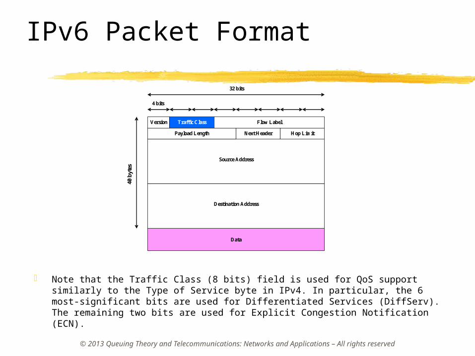
IPv6 Packet Format
Note that the Traffic Class (8 bits) field is used for QoS support similarly to the Type of Service byte in IPv4. In particular, the 6 most-significant bits are used for Differentiated Services (DiffServ). The remaining two bits are used for Explicit Congestion Notification (ECN).
© 2013 Queuing Theory and Telecommunications: Networks and Applications – All rights reserved
Version Traffic Class Flow Label
Payload Length
Source Address
Data
4 bits
32 bits
Next Header Hop Limit
Destination Address
40 b
ytes
IPv6 Deployment Strategy Any successful strategy for IPv6 deployment requires it to coexist with IPv4 for some extended time period. The following strategies have been developed to manage the transition from IPv4 to IPv6:
Dual-stack backbone: In dual-stack backbone deployment, all routers in the network maintain both IPv4 and IPv6 protocol stacks. Applications choose between IPv4 or IPv6.
IPv6 over IPv4 tunneling: IPv6 over IPv4 tunneling encapsulates IPv6 traffic in IPv4 packets to be sent over an IPv4 backbone. This solution enables IPv6 end systems and routers to communicate through an existing IPv4 infrastructure.
© 2013 Queuing Theory and Telecommunications: Networks and Applications – All rights reserved

© 2013 Queuing Theory and Telecommunications: Networks and Applications – All rights reserved
Thank you!
Related Documents