Lesson 4: Stationary stochastic processes · 3 the cross moment E(x t 1 x t2) depends only on t 1 t 2, that is cov(x t1;x t2) = cov(x t1+h;x ... strictly stationary but not weak stationary

Lesson 4: Stationary stochastic processes

Umberto Triacca

Dipartimento di Ingegneria e Scienze dell’Informazione e MatematicaUniversita dell’Aquila,

[email protected]

Umberto Triacca Lesson 4: Stationary stochastic processes

Stationary stochastic processes

Stationarity is a rather intuitive concept, it means that thestatistical properties of the process do not change over time.



There are two important forms of stationarity:

1 strong stationarity;

2 weak stationarity.



Strong stationarity concerns the shift-invariance (in time) of itsfinite-dimensional distributions.

Weak stationarity only concerns the shift-invariance (in time) offirst and second moments of a process.


Strongly stationary stochastic processes

Definition. The process {xt ; t ∈ Z} is strongly stationary if

Ft1+k,t2+k,··· ,ts+k(b1, b2, · · · , bs) = Ft1,t2,··· ,ts (b1, b2, · · · , bs)

for any finite set of indices {t1, t2, · · · , ts} ⊂ Z with s ∈ Z+, andany k ∈ Z.

Thus the process {xt ; t ∈ Z} is strongly stationary if the jointdistibution function of the vector (xt1+k , xt2+k , ..., xts+k) is equalwith the one of (xt1 , xt2 , ..., xts ) for for any finite set of indices{t1, t2, · · · , ts} ⊂ Z with s ∈ Z+, and any k ∈ Z.



The meaning of the strongly stationarity is that thedistribution of a number of random variables of thestochastic process is the same as we shift them along thetime index axis.



If {xt ; t ∈ Z} is a strongly stationary process, then

x1, x2, x3, ...

have the same distribution function.

(x1, x3), (x5, x7), (x9, x11), .....

have the same joint distribution function and further

(x1, x3, x5), (x7, x9, x11), (x13, x15, x17), ...

must have the same joint distribution function, and so on.



If the process is {xt ; t ∈ Z} is strongly stationary, then the jointprobability distribution function of (xt1 , xt2 , ..., xts ) is invariantunder translation.


iid process

An iid process is a strongly stationary process. This follows almostimmediate from the definition.

Since the random variables xt1+k , xt2+k , ..., xts+k are iid, we havethat

Ft1+k,t2+k,··· ,ts+k(b1, b2, · · · , bs) = F (b1)F (b2) · · ·F (bs)

On the other hand, also the random variables xt1 , xt2 , ..., xts are iidand hence

Ft1,t2,··· ,ts (b1, b2, · · · , bs) = F (b1)F (b2) · · ·F (bs).

We can conclude that

Ft1+k,t2+k,··· ,ts+k(b1, b2, · · · , bs) = Ft1,t2,··· ,ts (b1, b2, · · · , bs)


iid process

Remark. Let {xt ; t ∈ Z} be an iid process. We have that theconditional distribution of xT+h given values of (x1, ..., xT ) is

P(xT+h ≤ b|x1, ..., xT ) = P(xT+h ≤ b)

So the knowledge of the past has no value for predicting thefuture. An iid process is unpredictable.

Example. Under efficient capital market hypothesis, the stockprice change is an iid process. This means that the stock pricechange is unpredictable from previous stock price changes.



Consider the discrete stochastic process

{xt ; t ∈ N}

where xt = A, with A ∼ U (3, 7) (A is uniformly distributed on theinterval [3, 7]).

This process is of course strongly stationary.

Why?



Consider the discrete stochastic process

{xt ; t ∈ N}

where xt = tA, with A ∼ U (3, 7)

This process is not strongly stationary

Why?


Weakly stationary stochastic processes

If the second moment of xt is finite for all t, then the mean E (xt),the variance var(xt) = E [(xt − E (xt))2] = E (x2

t )− (E (xt))2 andthe covariance cov(xt1 , xt2) = E [(xt1 − E (xt1))(xt2 − E (xt2))] arefinite for all t, t1 and t2.

Why?

Hint: Use the Cauchy-Schwarz inequality|cov(x , y)|2 ≤ var(x)var(y)



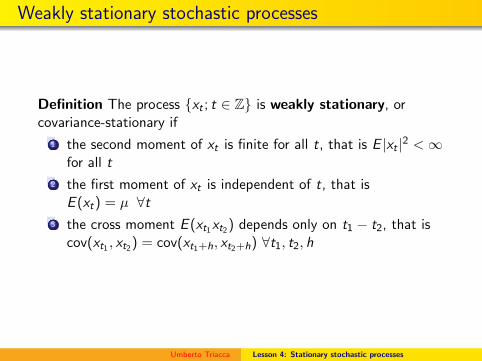
Definition The process {xt ; t ∈ Z} is weakly stationary, orcovariance-stationary if

1 the second moment of xt is finite for all t, that is E |xt |2 <∞for all t

2 the first moment of xt is independent of t, that isE (xt) = µ ∀t

3 the cross moment E (xt1xt2) depends only on t1 − t2, that iscov(xt1 , xt2) = cov(xt1+h, xt2+h) ∀t1, t2, h



Thus a stochastic process is covariance-stationary if

1 it has the same mean value, µ, at all time points;

2 it has the same variance, γ0, at all time points; and

3 the covariance between the values at any two time points,t, t − k, depend only on k, the difference between the twotimes, and not on the location of the points along the timeaxis.



An important example of covariance-stochastic process is theso-called white noise process.Definition . A stochastic process {ut ; t ∈ Z} in which the randomvariables ut , t = 0± 1,±2... are such that

1 E (ut) = 0 ∀t2 Var(ut) = σ2

u <∞ ∀t3 Cov(ut , ut−k) = 0 ∀t,∀k

is called white noise with mean 0 and variance σ2u, written

ut ∼WN(0, σ2u).

First condition establishes that the expectation is always constantand equal to zero. Second condition establishes that variance isconstant. Third condition establishes that the variables of theprocess are uncorrelated for all lags.If the random variables ut are independently and identicallydistributed with mean 0 and variance σ2

u then we will write

ut ∼ IID(0, σ2u)


White Noise process

Figure shows a possible realization of an IID(0,1) process.

Figure : A realization of an IID(0,1).


Random Walk process

An important example of weakly non-stationary stochasticprocesses is the following.Let

{yt ; t = 0, 1, 2, ...}

be a stochastic processs where y0 = δ <∞ and yt = yt−1 + ut fort = 1,2,..., with ut ∼WN(0, σ2

u).

This process is called random walk.


Random Walk process

The mean of yt is given by

E (yt) = δ

and its variance isVar(yt) = tσ2

u

Thus a random walk is not weakly stationary process.


Random Walk process

Figure shows a possible realization of a random walk.

Figure : A realization of a random walk.


Relation between strong and weak Stationarity

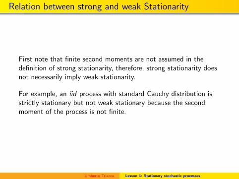
First note that finite second moments are not assumed in thedefinition of strong stationarity, therefore, strong stationarity doesnot necessarily imply weak stationarity.

For example, an iid process with standard Cauchy distribution isstrictly stationary but not weak stationary because the secondmoment of the process is not finite.



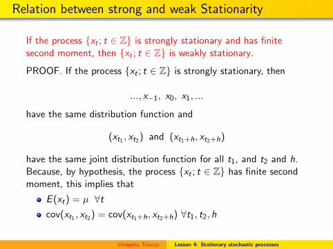
If the process {xt ; t ∈ Z} is strongly stationary and has finitesecond moment, then {xt ; t ∈ Z} is weakly stationary.

PROOF. If the process {xt ; t ∈ Z} is strongly stationary, then

..., x−1, x0, x1, ...

have the same distribution function and

(xt1 , xt2) and (xt1+h, xt2+h)

have the same joint distribution function for all t1, and t2 and h.Because, by hypothesis, the process {xt ; t ∈ Z} has finite secondmoment, this implies that

E (xt) = µ ∀tcov(xt1 , xt2) = cov(xt1+h, xt2+h) ∀t1, t2, h



Of course a weakly stationary process is not necessarily stronglystationary.

weak stationarity ; strong stationarity



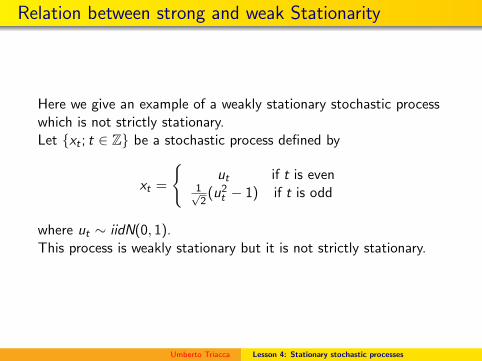
Here we give an example of a weakly stationary stochastic processwhich is not strictly stationary.Let {xt ; t ∈ Z} be a stochastic process defined by

xt =

{ut if t is even

1√2

(u2t − 1) if t is odd

where ut ∼ iidN(0, 1).This process is weakly stationary but it is not strictly stationary.



We have

E (xt) =

{E (ut) = 0 if t is even

1√2E (u2

t − 1) = 0 if t is odd

and

var(xt) =

{var(ut) = 1 if t is even

12 var(u2

t−1) = 1 if t is odd

Further, because xt and xt−k are independent random variables, wehave

cov(xt , xt−k) = 0 ∀k

Thus, the process xt is weakly stationary. In particular,xt ∼WN(0, 1).



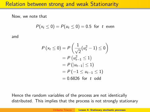
Now, we note that

P(xt ≤ 0) = P(ut ≤ 0) = 0.5 for t even

and

P (xt ≤ 0) = P

(1√2

(u2t − 1) ≤ 0

)= P

(u2t−1 ≤ 1

)= P (|ut−1| ≤ 1)

= P (−1 ≤ ut−1 ≤ 1)

= 0.6826 for t odd

Hence the random variables of the process are not identicallydistributed. This implies that the process is not strongly stationary



There is one important case however in which weak stationarityimplies strong stationarity.

If {xt ; t ∈ Z} is a weakly stationary Gaussian stochastic process,then {xt ; t ∈ Z} is strongly stationary.

Why?



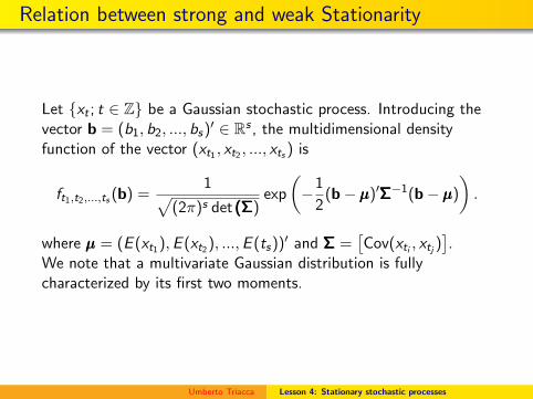
Let {xt ; t ∈ Z} be a Gaussian stochastic process. Introducing thevector b = (b1, b2, ..., bs)′ ∈ Rs , the multidimensional densityfunction of the vector (xt1 , xt2 , ..., xts ) is

ft1,t2,...,ts (b) =1√

(2π)s det (Σ(Σ(Σ)exp

(−1

2(b−µµµ)′ΣΣΣ−1(b−µµµ)

).

where µµµ = (E (xt1),E (xt2), ...,E (ts))′ and ΣΣΣ =[Cov(xti , xtj )

].

We note that a multivariate Gaussian distribution is fullycharacterized by its first two moments.



Let {xt ; t ∈ Z} be a Gaussian stochastic process. Assume that theprocess is weakly stationary. If the process i weakly stationary,then

1 E (xt) = µ ∀t2 Var(xt) = γ0 <∞ ∀t3 Cov(xt1+k , xt2+k) = Cov(xt1 , xt2) ∀t1, t2, ∀k

and henceft1+k,t2+k,...,ts+k(b) = ft1,t2,...,ts (b)

It follows that the joint distibution function of the vector(xt1+k , xt2+k , ..., xts+k) is equal with the one of (xt1 , xt2 , ..., xts ) forfor any finite set of indices {t1, t2, · · · , ts} ⊂ Z with s ∈ Z+, andany k ∈ Z. This implies that the process {xt ; t ∈ Z} is stronglystationary.



Conversely, if {xt ; t ∈ Z} is a Gaussian strongly stationarystochastic process, then it is weakly stationary because it has finitevariance.Thus we can conclude that in the case of Gaussian stochasticprocess, the two definitions of stationarity are equivalent.


White Noise process

We note that a white noise process is not necessarily stronglystationary. Let w be a random variable uniformly distributed in theinterval (0; 2π). We consider the process {Zt ; t = 1, 2, ...} definedby

Zt = cos(tw) t = 1, 2, ...

We have that

1 E (Zt) = 0 ∀t2 Var(Zt) = 1

2 ∀t3 Cov(Zt ,Zt−k) = 0 ∀t, ∀k

Thus Zt ∼WN(0, .5). However, it can be shown that is notstrongly stationary.


Lesson 4: Stationary stochastic processes · 3 the cross moment E(x t 1 x t2) depends only on t 1 t 2, that is cov(x t1;x t2) = cov(x t1+h;x ... strictly stationary but not weak stationary

Documents