Univariate time series Multivariate time series Panels Advanced Econometrics Based on the textbook by Verbeek: A Guide to Modern Econometrics Robert M. Kunst [email protected] University of Vienna and Institute for Advanced Studies Vienna May 2, 2013 Advanced Econometrics University of Vienna and Institute for Advanced Studies Vienna

Welcome message from author
This document is posted to help you gain knowledge. Please leave a comment to let me know what you think about it! Share it to your friends and learn new things together.
Transcript
Univariate time series Multivariate time series Panels
Advanced Econometrics
Based on the textbook by Verbeek:A Guide to Modern Econometrics
Robert M. [email protected]
University of Vienna
and
Institute for Advanced Studies Vienna
May 2, 2013
Advanced Econometrics University of Vienna and Institute for Advanced Studies Vienna

Univariate time series Multivariate time series Panels
Outline
Univariate time series
Multivariate time seriesGeneral conceptsCointegrationVector autoregressionsMultivariate cointegration
Panels
Advanced Econometrics University of Vienna and Institute for Advanced Studies Vienna

Univariate time series Multivariate time series Panels
Advanced Econometrics University of Vienna and Institute for Advanced Studies Vienna
Univariate time series Multivariate time series Panels
General concepts
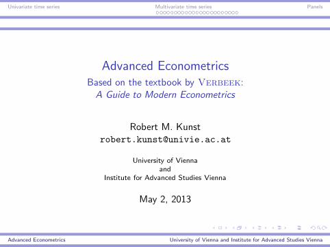
Issues with multivariate time series
◮ Regressing integrated variables on other integrated variablesoften yields apparently significant coefficients (even if there isno relation) and integrated residuals: spurious regression;
◮ If residuals are stationary, the relation may be an importantdynamic equilibrium: cointegration;
◮ Cointegration is closely related to the dynamic mechanismthat is directed toward the equilibrium: error correction;
◮ The multivariate generalization of the autoregressive model isthe vector autoregression (VAR), which sets a convenientframe for cointegration, causality etc.
Advanced Econometrics University of Vienna and Institute for Advanced Studies Vienna

Univariate time series Multivariate time series Panels
General concepts
A simple dynamic model
Consider two stationary variables Y and X , with X regarded asexogenous, related by an autoregressive distributed lags (ARDL)model
Yt = δ + θYt−1 + φ0Xt + φ1Xt−1 + εt ,
with white-noise εt and |θ| < 1. The entity
∂Yt
∂Xt
= φ0
is called the impact multiplier.
Advanced Econometrics University of Vienna and Institute for Advanced Studies Vienna
Univariate time series Multivariate time series Panels
General concepts
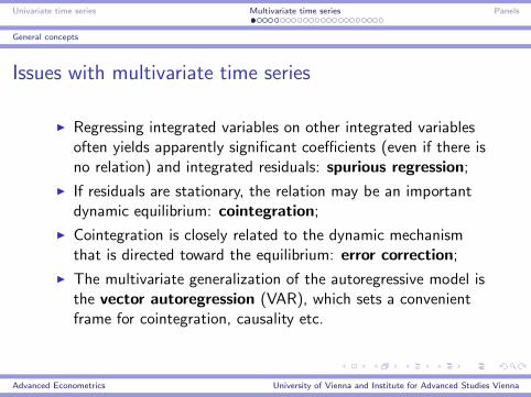
The equilibrium multiplier
Straightforward evaluation yields
∂Yt+1
∂Xt
= θφ0 + φ1
and∂Yt+2
∂Xt
= θ∂Yt+1
∂Xt
= θ(θφ0 + φ1)
The sum of all these multipliers describes the long-run effect
∞∑
j=0
∂Yt+j
∂Xt
= φ0 +θφ0 + φ1
1− θ=
φ0 + φ1
1− θ,
the long-run multiplier or equilibrium multiplier β.
Advanced Econometrics University of Vienna and Institute for Advanced Studies Vienna

Univariate time series Multivariate time series Panels
General concepts
Error correction
X and Y are stationary, for this reason
E(Yt) =δ
1− θ+ βE(Xt) = α+ βE(Xt)
for some constant α. Some manipulation yields
∆Yt = φ0∆Xt − (1− θ)(Yt−1 − α− βXt−1) + εt ,
an error-correction model: Y adjusts to deviations fromequilibrium, with 1− θ representing the intensity of adjustment.
Advanced Econometrics University of Vienna and Institute for Advanced Studies Vienna

Univariate time series Multivariate time series Panels
General concepts
Generalizations to higher lag orders
Assume the general form
θ(L)Yt = δ + φ(L)Xt + εt ,
with lag polynomials of orders p and q and invertible θ(z).Applying the inverse operator θ−1(L) yields
Yt = θ−1(L)φ(L)Xt + θ−1(L)εt ,
and the long-run multiplier becomes
θ−1(1)φ(1) =φ0 + φ1 + . . .+ φq
1− θ1 − . . .− θp,
with the denominator positive because of stability.
Advanced Econometrics University of Vienna and Institute for Advanced Studies Vienna

Univariate time series Multivariate time series Panels
Cointegration
The basic experiment of spurious regression
Presume Xt and Yt are independent random walks. The regression
Yt = α+ βXt + error
tends to produce significant coefficients and non-zero R2. Flankingdiagnostics such as the Durbin-Watson statistic tend to indicatethat something is wrong. In fact, the residual is I(1) byconstruction.
To avoid spurious regression, first subject Y and X to unit-roottests. If these tests support the null of I(1), test residuals. Ifunit-root tests on residuals fail to reject, we have a spuriousregression problem. Note, however, that the usual Dickey-Fullersignificance points are invalid for residual unit-root tests.
Advanced Econometrics University of Vienna and Institute for Advanced Studies Vienna
Univariate time series Multivariate time series Panels
Cointegration
Non-spurious regression with integrated variables
Consider two I(1) variables Yt and Xt , with Yt − βXt stationaryI(0). Then, Y and X are said to be cointegrated. The regression
Yt = α+ βXt + error
yields a coefficient estimate β̂ that is super-consistent for β, i.e.
√T (β̂ − β) → 0, T (β̂ − β) ⇒ D,
with a non-standard limit distribution D. Note that errors are I(0)but they are usually not white noise here. This regression is calleda cointegrating regression.
Advanced Econometrics University of Vienna and Institute for Advanced Studies Vienna

Univariate time series Multivariate time series Panels
Cointegration
Cointegration with two variables
DefinitionIf Yt and Xt are both I(1) and there exists a β such thatZt = Yt − βXt is I(0), then X and Y are cointegrated and(1,−β)′ is the cointegrating vector.
The cointegrating relation can be interpreted as a long-runequilibrium in a non-stationary dynamic model, and the model canalso be written as an error-correction model (see below).
Advanced Econometrics University of Vienna and Institute for Advanced Studies Vienna
Univariate time series Multivariate time series Panels
Cointegration
Testing for cointegration in a simple regression
In order to determine whether the regression is spurious orcointegrating, it is recommended to first test X and Y for unitroots. If the unit-root tests fail to reject, run the regression (nolags!) and apply unit-root tests to residuals. Use differentsignificance points from the usual DF test. Appropriate significancepoints have been calculated by Phillips & Ouliaris, forexample.
◮ If the residual unit-root test rejects, there is evidence oncointegration;
◮ If the residual unit-root test fails to reject, the regression isspurious.
Advanced Econometrics University of Vienna and Institute for Advanced Studies Vienna

Univariate time series Multivariate time series Panels
Cointegration
Cointegration and error correction
Engle & Granger have shown that, if X and Y arecointegrated, then there exists an error-correction representation
θ(L)∆Yt = δ + φ(L)∆Xt−1 − γZt−1 + α(L)εt ,
with Zt = Yt − βXt . If Y deviates positively from the equilibriumat t − 1, ∆Y corrects back to it at t by being smaller than usual,and similarly for negative deviations. X could also adjust, but thiscan only be captured in a full multivariate model.
Advanced Econometrics University of Vienna and Institute for Advanced Studies Vienna

Univariate time series Multivariate time series Panels
Vector autoregressions
Vector autoregressions: the concept
The vector autoregressive model (VAR) is a multivariategeneralization of the univariate AR model: variables are vectors,coefficients are matrices:
Yt = δ +Θ1Yt−1 + . . .+ΘpYt−p + εt ,
with Yt ,Yt−1, . . . ,Yt−p , εt , δ k–vectors and Θj , j = 1, . . . , pk × k–matrices. The lag polynomial is now a matrix polynomial
Θ(L) = Ik −Θ1L− . . .−ΘpLp,
with Ik denoting the k–dimensional identity matrix. In short, wewrite
Θ(L)Yt = εt .
Advanced Econometrics University of Vienna and Institute for Advanced Studies Vienna
Univariate time series Multivariate time series Panels
Vector autoregressions
Stationarity of multivariate processes
In analogy to the univariate case, the vector variable Yt is said tobe (covariance) stationary, iff
◮ EYt = µ = (µ1, . . . , µk)′;
◮ E(Yt − µ)(Yt − µ)′ = varYt = ΣY ;
◮ E(Yt − µ)(Yt−h − µ)′ = cov(Yt ,Yt−h) = Γ(h).
The matrix-valued function Γ(h) is the cross-covariance function,its standardized version is the cross-correlation function (CCF). Itis skew symmetric, i.e. Γ(h)′ = Γ(−h). Also note that Γ(0) = ΣY .
Advanced Econometrics University of Vienna and Institute for Advanced Studies Vienna
Univariate time series Multivariate time series Panels
Vector autoregressions
Multivariate white noise
A k–dimensional variable (εt) is said to be white noise, iff
◮ εt is stationary;
◮ Eεt = (0, . . . , 0)′;
◮ Γ(h) = 0 for h 6= 0.
Note that component j is uncorrelated with k at all leads and lags,but typically correlated simultaneously, i.e. Σε is not usuallydiagonal.
Advanced Econometrics University of Vienna and Institute for Advanced Studies Vienna

Univariate time series Multivariate time series Panels
Vector autoregressions
Stability of the VAR
O.c.s. that the VAR is stable iff all solutions (roots) ζ of the(scalar) determinantal polynomial equation
detΘ(L) = 0
fulfill the condition |ζ| > 1. Then, it makes sense to consider theinfinite-order MA representation
Yt = Θ(1)−1δ +Θ(L)−1εt = µ+ A(L)εt .
Advanced Econometrics University of Vienna and Institute for Advanced Studies Vienna

Univariate time series Multivariate time series Panels
Vector autoregressions
The impulse response function
The coefficient matrices of the MA representation of a VAR can beinterpreted as derivatives
Ah =∂Yt+h
∂ε′t,
and thus as indicating the response in the components of Y to‘shocks’ in the components of the error process ε. For this reason,the k2 components of the function A(h) are called theimpulse-response function.
A(h) does not really indicate the response to shocks in thecomponents of past variables Y , due to dynamic feedback. A(h)also fails to reflect the immediate response of other components inε, as Σε is not generally diagonal.
Advanced Econometrics University of Vienna and Institute for Advanced Studies Vienna
Univariate time series Multivariate time series Panels
Multivariate cointegration
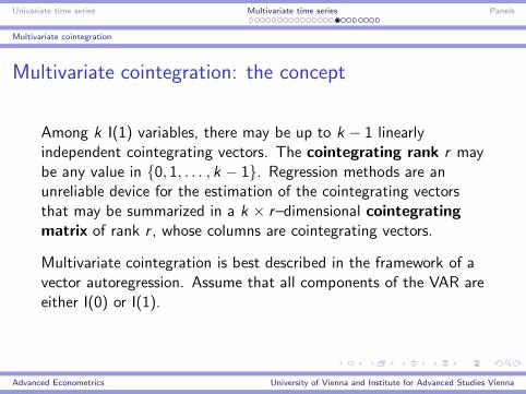
Multivariate cointegration: the concept
Among k I(1) variables, there may be up to k − 1 linearlyindependent cointegrating vectors. The cointegrating rank r maybe any value in {0, 1, . . . , k − 1}. Regression methods are anunreliable device for the estimation of the cointegrating vectorsthat may be summarized in a k × r–dimensional cointegratingmatrix of rank r , whose columns are cointegrating vectors.
Multivariate cointegration is best described in the framework of avector autoregression. Assume that all components of the VAR areeither I(0) or I(1).
Advanced Econometrics University of Vienna and Institute for Advanced Studies Vienna

Univariate time series Multivariate time series Panels
Multivariate cointegration
Error-correction representation of VAR
Every VAR of order p
Yt = δ +Θ1Yt−1 + . . .+ΘpYt−p + εt
can be re-written as a vector error-correction model (VECM)
∆Yt = δ + Γ1∆Yt−1 + . . . + Γp−1∆Yt−p+1 + ΠYt−1 + εt ,
with matrices Γj and Π being functions of Θ1, . . . ,Θp , in particular
Π = −Ik +Θ1 + . . .+Θp = −Θ(1)
for the long-run matrix Π, which represents all cointegrationfeatures in the system.
Advanced Econometrics University of Vienna and Institute for Advanced Studies Vienna
Univariate time series Multivariate time series Panels
Multivariate cointegration
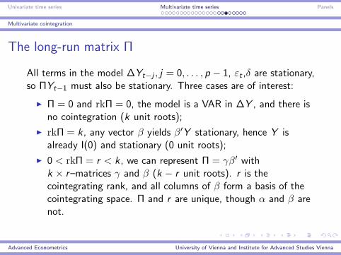
The long-run matrix Π
All terms in the model ∆Yt−j , j = 0, . . . , p − 1, εt ,δ are stationary,so ΠYt−1 must also be stationary. Three cases are of interest:
◮ Π = 0 and rkΠ = 0, the model is a VAR in ∆Y , and there isno cointegration (k unit roots);
◮ rkΠ = k , any vector β yields β′Y stationary, hence Y isalready I(0) and stationary (0 unit roots);
◮ 0 < rkΠ = r < k , we can represent Π = γβ′ withk × r–matrices γ and β (k − r unit roots). r is thecointegrating rank, and all columns of β form a basis of thecointegrating space. Π and r are unique, though α and β arenot.
Advanced Econometrics University of Vienna and Institute for Advanced Studies Vienna

Univariate time series Multivariate time series Panels
Multivariate cointegration
No drift in the system
Take expectations on the VECM form (∆Y is stationary):
(I − Γ1 − . . .− Γp)E∆Yt = δ + γE(β′Yt−1) + Eεt
If there is no linear trend in any Y component, the l.h.s. is 0, andso is the r.h.s., which implies that δ is proportional to γ or
δ = −γα,
which yields the VECM with restricted intercepts
∆Yt = γ(−α+ β′Yt−1) + Γ1∆Yt−1 + . . .+ Γp−1∆Yt−p+1 + εt .
Advanced Econometrics University of Vienna and Institute for Advanced Studies Vienna
Univariate time series Multivariate time series Panels
Multivariate cointegration
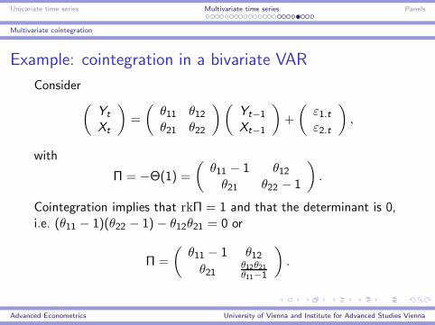
Example: cointegration in a bivariate VAR
Consider(
Yt
Xt
)
=
(
θ11 θ12θ21 θ22
)(
Yt−1
Xt−1
)
+
(
ε1.tε2.t
)
,
with
Π = −Θ(1) =
(
θ11 − 1 θ12θ21 θ22 − 1
)
.
Cointegration implies that rkΠ = 1 and that the determinant is 0,i.e. (θ11 − 1)(θ22 − 1)− θ12θ21 = 0 or
Π =
(
θ11 − 1 θ12θ21
θ12θ21θ11−1
)
.
Advanced Econometrics University of Vienna and Institute for Advanced Studies Vienna

Univariate time series Multivariate time series Panels
Multivariate cointegration
Example: the bivariate VECM
For the bivariate VECM, we obtain
(
∆Yt
∆Xt
)
=
(
1θ21
θ11−1
)
{(θ11 − 1)Yt−1 + θ12Xt−1}+(
ε1.tε2.t
)
,
with the recognizable cointegrating vector (θ11 − 1, θ12) = β′. Onecan check that (θ11 − 1)Yt + θ12Xt is stationary. Note thatγ = (θ11 − 1, θ21)
′ and β = (1, θ12θ11−1
)′ would also work.
Advanced Econometrics University of Vienna and Institute for Advanced Studies Vienna
Univariate time series Multivariate time series Panels
Multivariate cointegration
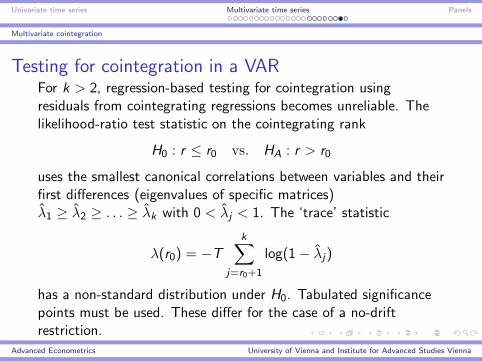
Testing for cointegration in a VARFor k > 2, regression-based testing for cointegration usingresiduals from cointegrating regressions becomes unreliable. Thelikelihood-ratio test statistic on the cointegrating rank
H0 : r ≤ r0 vs. HA : r > r0
uses the smallest canonical correlations between variables and theirfirst differences (eigenvalues of specific matrices)λ̂1 ≥ λ̂2 ≥ . . . ≥ λ̂k with 0 < λ̂j < 1. The ‘trace’ statistic
λ(r0) = −T
k∑
j=r0+1
log(1− λ̂j)
has a non-standard distribution under H0. Tabulated significancepoints must be used. These differ for the case of a no-driftrestriction.
Advanced Econometrics University of Vienna and Institute for Advanced Studies Vienna

Univariate time series Multivariate time series Panels
Multivariate cointegration
Recommended steps for the ‘Johansen procedure’
1. Make sure that all component variables are either I(0) or I(1).The procedure works if some variables are stationary.
2. Determine a lag order p for the VAR, e.g. by AIC.
3. Decide whether to use the no-trend restriction.
4. Determine the cointegrating rank by the trace test sequence,using a VAR with p lags.
5. Use the estimates for all coefficients from a VECM estimationthat uses the rank r and p − 1 augmenting lags. This stepyields γ̂ and the cointegrating vector(s) β̂, among others.
Why not estimate the cointegrating vector from a regression afterstep 4? This is much less efficient.
Advanced Econometrics University of Vienna and Institute for Advanced Studies Vienna

Univariate time series Multivariate time series Panels
Advanced Econometrics University of Vienna and Institute for Advanced Studies Vienna
Related Documents