Les Houches "Physics at TeV Colliders 2005'' Beyond the Standard Model working group:summary report

arX

iv:h

ep-p

h/06

0219

8v1

21

Feb

200

6

LES HOUCHES “PHYSICS AT TEV COLLIDERS 2005”BEYOND THE STANDARD MODEL WORKING GROUP:SUMMARY REPORT

B.C. Allanach1, C. Grojean2,3, P. Skands4, E. Accomando5, G. Azuelos6,7, H. Baer8,C. Balazs9, G. Belanger10, K. Benakli11, F. Boudjema10, B. Brelier6, V. Bunichev12,G. Cacciapaglia13, M. Carena4, D. Choudhury14, P.-A. Delsart6, U. De Sanctis15, K. Desch16,B.A. Dobrescu4, L. Dudko12, M. El Kacimi17, U. Ellwanger18, S. Ferrag19, A. Finch20,F. Franke21, H. Fraas21, A. Freitas22, P. Gambino5, N. Ghodbane3, R.M. Godbole23,D. Goujdami17, Ph. Gris24, J. Guasch25, M. Guchait26, T. Hahn27, S. Heinemeyer28,A. Hektor29, S. Hesselbach30, W. Hollik27, C. Hugonie31, T. Hurth3,32, J. Idarraga6,O. Jinnouchi33, J. Kalinowski34, J.-L. Kneur31, S. Kraml3, M. Kadastik29, K. Kannike29,R. Lafaye3,35, G. Landsberg36, T. Lari15, J. S. Lee37, J. Lykken4, F. Mahmoudi38, M. Mangano3,A. Menon9,39, D.J. Miller40, T. Millet 41, C. Milstene4, S. Montesano15, F. Moortgat3,G. Moortgat-Pick3, S. Moretti42,43, D.E. Morrissey44, S. Muanza4,41,45, M.M. Muhlleitner3,10,M. Muntel29, H. Nowak46, T. Ohl21, S. Penaranda3, M. Perelstein13, E. Perez46,47, S. Perries41,M. Peskin31, J. Petzoldt20, A. Pilaftsis48, T. Plehn27,49, G. Polesello50, A. Pompos51, W. Porod52,H. Przysiezniak35, A. Pukhov53, M. Raidal29, D. Rainwater54, A.R. Raklev55, J. Rathsman30,J. Reuter56, P. Richardson57, S.D. Rindani58, K. Rolbiecki34, H. Rzehak59, M. Schumacher60,S. Schumann61, A. Semenov62, L. Serin45, G. Servant2,3, C.H. Shepherd-Themistocleous42,S. Sherstnev53, L. Silvestrini63, R.K. Singh23, P. Slavich10, M. Spira59, A. Sopczak20,K. Sridhar26 L. Tompkins45,64, C. Troncon15, S. Tsuno65, K. Wagh23, C.E.M. Wagner9,39,G. Weiglein57, P. Wienemann16, D. Zerwas45, V. Zhukov66,67.

Editors of proceedings in boldconvenorof Beyond the Standard Modelworking group1 DAMTP, CMS, Wilberforce Road, Cambridge, CB3 0WA, UK2 SPhT, CEA-Saclay, Orme des Merisiers, F-91191 Gif-sur-Yvette Cedex, France3 Physics Department, CERN, CH-1211 Geneva 23, Switzerland4 Fermilab (FNAL), PO Box 500, Batavia, IL 60510, USA5 INFN, Sezione di Torino and Universita di Torino, Dipartimento di Fisica Teorica, Italy6 Universite de Montreal, Canada7 TRIUMF, Vancouver, Canada8 Department of Physics, Florida State University, Tallahassee, FL 32306, USA9 HEP Division, Argonne National Laboratory, 9700 Cass Ave.,Argonne, IL 60449, USA10 LAPTH, 9 Chemin de Bellevue, B.P. 110, Annecy-le-Vieux 74941, France11 LPTHE, Universites de Paris VI et VII, France12 Moscow State University, Russia13 Institute for High Energy Phenomenology, Cornell University, Ithaca, NY 14853, USA14 Department of Physics and Astrophysics, University of Delhi, Delhi 110 007, India15 Universita di Milano - Dipartimento di Fisica and IstitutoNazionale di Fisica Nucleare -Sezione di Milano, Via Celoria 16, I-20133 Milan, Italy16 Albert-Ludwigs Universitat Freiburg, Physikalisches Institut, Hermann-Herder Str. 3,D-79104 Freiburg, Germany17 Universite Cadi Ayyad, Faculte des Sciences Semlalia, B.P. 2390, Marrakech, Maroc

2

18 LPT, Universite de Paris XI, Bat. 210, F-91405 Orsay Cedex, France19 Department of Physics, University of Oslo,Oslo, Norway20 Lancaster University, Lancaster LA1 4YB, UK21 Institut fur Theoretische Physik und Astrophysik, Universitat Wurzburg, Germany22 Institute for Theoretical Physics, Univ. of Zurich, CH-8050 Zurich, Switzerland23 Indian Institute of Science, IISc, Bangalore, 560012, India24 LPC Clermont-Ferrand, Universite Blaise Pascal, France25 Departament d’Estructura i Constituents de la Materia, Facultat de Fısica, Universitat deBarcelona, Diagonal 647, E-08028 Barcelona, Catalonia, Spain26 Tata Institute of Fundamental Research, Homi Bhabha Road, Mumbai 400005, India27 MPI fur Physik, Werner-Heisenberg-Institut, D–80805 Munchen, Germany28 Depto. de Fisica Teorica, Universidad de Zaragoza, 50009 Zaragoza, Spain29 National Institute of Chemical Physics and Biophysics, Ravala 10, Tallinn 10144, Estonia30 High Energy Physics, Uppsala University, Box 535, S-751 21 Uppsala, Sweden31 LPTA, UMR5207-CNRS, Universite Montpellier II, F-34095 Montpellier Cedex 5, France32 SLAC, Stanford University, Stanford, California 94409 USA33 Physics Div. 2, Institute of Particle and Nuclear Studies, KEK, Tsukuba Japan34 Instytut Fizyki Teoretycznej, Uniwersytet Warszawski, PL-00681 Warsaw, Poland35 LAPP, 9 Chemin de Bellevue, B.P. 110, Annecy-le-Vieux 74941, France36 Brown University, Providence, Rhode Island, USA37 CTP, School of Physics, Seoul National University, Seoul 151-747, Korea38 Physics Department, Mount Allison University, Sackville NB, E4L 1E6 Canada39 Enrico Fermi Institute, University of Chicago, 5640 S. Ellis Ave., Chicago, IL 60637, USA40 Department of Physics and Astronomy, University of Glasgow, Glasgow G12 8QQ, UK41 IPN Lyon, 69622 Villeurbanne, France42 School of Physics and Astronomy, University of Southampton, SO17 1BJ, UK43 Particle Physics Division, Rutherford Appleton Laboratory, Oxon OX11 0QX, UK44 Department of Physics, University of Michigan, Ann Arbor, MI 48109, USA45 LAL, Universite de Paris-Sud, Orsay Cedex, France46 Deutsches Elektronen-Synchrotron DESY, D–15738 Zeuthen,Germany47 SPP, DAPNIA, CEA-Saclay, F-91191 Gif-sur-Yvette Cedex, France48 School of Physics and Astronomy, University of Manchester,Manchester M13 9PL, UK49 University of Edinburgh, GB50 INFN, Sezione di Pavia, Via Bassi 6, I-27100 Pavia, Italy51 University of Oklahoma, USA52 Instituto de Fısica Corpuscular, C.S.I.C., Valencia, Spain53 Skobeltsyn Inst. of Nuclear Physics, Moscow State Univ., Moscow 119992, Russia54 Dept. of Physics and Astronomy, University of Rochester, NY, USA55 Dept. of Physics and Technology, University of Bergen, N-5007 Bergen, Norway56 DESY Theory Group, Notkestr. 85, D-22603 Hamburg, Germany57 IPPP, University of Durham, Durham DH1 3LE, UK58 Physical Research Laboratory, Ahmedabad, India59 Paul Scherrer Institut, CH–5232 Villigen PSI, Switzerland60 Zweites Physikalisches Institut der Universitat, D-37077 Gottingen, Germany61 Institute for Theoretical Physics, TU Dresden, 01062, Germany62 Joint Institute for Nuclear Research (JINR), 143980, Dubna, Russia63 INFN, Sezione di Roma and Universita di Roma “La Sapienza”,I-00185 Rome, Italy

64 University of California, Berkeley, USA65 Department of Physics, Okayama University, Okayama, 700-8530, Japan66 IEKP, Universitat Karlsruhe (TH), P.O. Box 6980, 76128 Karlsruhe, Germany67 SINP, Lomonosov Moscow State University, 119992 Moscow , Russia

AbstractThe work contained herein constitutes a report of the “Beyond the Stan-dard Model” working group for the Workshop “Physics at TeV Collid-ers”, Les Houches, France, 2–20 May, 2005. We present reviews ofcurrent topics as well as original research carried out for the workshop.Supersymmetric and non-supersymmetric models are studied, as wellas computational tools designed in order to facilitate their phenomenol-ogy.

Acknowledgements

We would like to heartily thank the funding bodies, organisers, staff and other participants of theLes Houches workshop for providing a stimulating and livelyenvironment in which to work.

4

Contents

BSM SUSY 8

1 BSM SUSY 8

2 Focus-Point studies with the ATLAS detector 11

3 SUSY parameters in the focus point-inspired case 18

4 Validity of the Barr neutralino spin analysis at the LHC 24

5 The trilepton signal in the focus point region 28

6 Constraints on mSUGRA from indirect DM searches 33

7 Relic density of dark matter in the MSSM with CP violation 39

8 Light scalar top quarks 45

9 Neutralinos in combined LHC and ILC analyses 73

10 Electroweak observables and split SUSY at future colliders 78

11 Split supersymmetry with Dirac gaugino masses 84

12 A search for gluino decays intobb+ ℓ+ℓ− at the LHC 90

13 Sensitivity of the LHC to CP violating Higgs bosons 96

14 Testing the scalar mass universality of mSUGRA at the LHC 100

5

TOOLS 104

15 A repository for beyond-the-Standard-Model tools 104

16 Status of the SUSY Les Houches Accord II project 114

17 Pythia UED 127

18 Les Houches squared event generator for the NMSSM 135

19 The MSSM implementation in SHERPA 140

20 Calculations in the MSSM Higgs sector withFeynHiggs2.3 142

21 micrOMEGAs2.0 and the relic density of dark matter 146

NON-SUSY BSM 151

22 NON SUSY BSM 151

23 Universal extra dimensions at hadron colliders 153

24 KK states at the LHC in models with localized fermions 158

25 Kaluza–Klein dark matter: a review 164

26 The Higgs boson as a gauge field 174

27 Little Higgs models: a Mini-Review 183

28 The Littlest Higgs andΦ++ pair production at LHC 191

6

29 Polarization in third family resonances 197

30 Charged Higgs boson studies at the Tevatron and LHC 206

31 Diphoton production at the LHC in the RS model 217

32 Higgsless models of electroweak symmetry breaking 223

33 Vector boson scattering at the LHC 235

BSM SUSY

8

Part 1

BSM SUSYB.C. Allanach

On the eve before Large Hadron Collider (LHC) data taking, there are many excitingprospects for the discovery and measurement of beyond the Standard Model physics in general,and weak-scale supersymmetry in particular. It is also always important to keep in mind the po-tential benefits (or pitfalls) of a future ILC in the event that SUSY particles are discovered at theLHC. The precision from the ILC will be invaluable in terms ofpinning down supersymmetry(SUSY) breaking, spins, coupling measurements as well as identifying dark matter candidates.These arguments apply to several of the analyses contained herein, but often also apply to othernon-SUSY measurements (and indeed are required for model discrimination).

At the workshop, several interesting analysis strategies were developed for particular rea-sons in different parts of SUSY parameter space. The focus-point region has heavy scalars and alightest neutralino that has a significant higgsino component leading to a relic dark matter candi-date that undergoes efficient annihilation into weak gauge boson pairs, leading to predictions ofrelic density in agreement with the WMAP/large scale structure fits. It is clear that LHC discov-ery and measurement of the focus point region could be problematic due to the heavy scalars.However, in Part 2, it is shown how a multi-jet+missing energy signature at the LHC selectsgluino pairs in this scenario, discriminating against background as well as contamination fromweak gaugino production. Gauginos can have light masses andtherefore sizable cross-sectionsin the focus-point region. The di-lepton invariant mass distribution also helps in measuring theSUSY masses. An International Linear Collider (ILC) could measure the low mass gauginosextremely precisely in the focus point region, and data fromcross-sections, forward backwardasymmetries can be added to those from the LHC in order to constrain the masses of the heavyscalars. This idea is studied in Part 3.

Of course, assuming the discovery of SUSY-like signals at the LHC, and before the adventof an ILC, we can ask the question: how may we know the theory isSUSY? Extra-dimensionalmodels (Universal Extra Dimensions), as well as little Higgs models with T-parity, can givethe same final states and cascade decays. One important smoking gun of SUSY is the sparticlespin. Measuring the spin at the LHC is a very challenging prospect, but nevertheless therehas been progress made by Barr, who constructed a charge asymmetric invariant mass for spindiscrimination in the cascade decays. In Part 4, it is shown that such an analysis has a ratherlimited applicability to SUSY breaking parameter space, flagging the fact that further efforts tomeasure spins would be welcome.

There is a tantalising signal from the EGRET telescope on excess diffuse gamma produc-tion in our galaxy and at energies of around 100 GeV. This has been interpreted as the result ofSUSY dark matter annihilation into photons. Backgrounds inthe flux are somewhat uncertain,but the signal correlates with dark matter distributions inferred from rotation curves, addingadditional interest. If the EGRET signal is indeed due to SUSY dark matter, it is interesting toexamine the implications for colliders. The tri-lepton signals at the Tevatron and at the LHC isinvestigated in Part 5 for an EGRET-friendly point. A combined fit to mSUGRA is aided bymeasurements of neutral Higgs masses, and yields acceptable precision, although some work isrequired to reduce theoretical uncertainties. In Part 6, gaugino production is studied at the LHC,

9

and gives large signals due to the light gauginos (assuming gaugino universality). The EGRETregion is compatible with other constraints, such as the inferred cosmological dark matter relicdensity and LEP2 bounds uponmh0 etc. 30 fb−1 should be enough integrated luminosity toprobe the EGRET-friendly region of parameter space.

The calculations of the relic density of thermal neutralinodark matter are being extendedto cover CP violation in the MSSM. This obviously generalises the usual CP-conserving casesstudied and could be important particularly if SUSY is responsible for baryogenesis, which re-quires CP-violation as one of the Sakharov conditions. The effects of phases is examined inPart 7 in regions of parameter space where higgs-poles annihilate much of the dark matter. Therelationship between relevant particle masses and relic density changes - this could be an impor-tant feature to take into account if trying to check cosmology by using collider measurementsto predict the current density, and comparing with cosmological/astrophysical observation.

As well as providing dark matter, supersymmetry could produce the observed baryonasymmetry in the unvierse, provided stop squarks are ratherlight and there is a significantamount of CP violation in the SUSY breaking sector. The experimental verification of this ideais explored in Part 8 where stop decays into charm and neutralino at the LHC are discussed.Four baryogenesis benchmark points are defined for future investigation. Light heavily mixedstops can be produced at the LHC, sometimes in association with a higgs boson and the resultingsignature is examined. Finally, it is shown that quasi-degenerate top/stops (often expected inMSSM baryogenesis) can be disentangled at the ILC despite c-quark tagging challenges.

In Part 9, it is investigated how non-minimal charginos and neutralinos (when a gaugesinglet is added to the MSSM in order to address the supersymmetricµ problem) may be iden-tified by combining ILC and LHC information on their masses and cross-sections. Split SUSYhas the virtue of being readily ruled out at the LHC. In split SUSY, one forgets the technical hi-erarchy problem (reasoning that perhaps there is an anthropic reason for it), allowing the scalarsto be ultra-heavy, ameliorating the SUSY flavour problem. The gauginos are kept light in orderto provide dark matter and gauge unification. We would like toargue that the Standard Modelplus axion dark matter (and no single-step gauge unification) is preferred by the principle ofOccam’s razor if one can forget the technical hierarchy problem. Given the intense interest inthe literature on split SUSY, this appears to be a minority view, however. In Part 10, constraintsfrom the precision electroweak variablesMW andsin2 θeff are used to constrain split SUSY.It is found that the GigaZ option of the ILC is required to measure the loop effects from splitSUSY. As shown in Part 11, split SUSY is predicted in a deformed intersecting brane model.

In Part 12, gluino decays through sbottom squarks are investigated at the LHC. Infor-mation on bottom squarks could be important for constraining tan β and the trilinear scalarcoupling, for instance. The signal is somewhat complex: 2b’s, one quark jet, opposite signsame flavour leptons and the ubiquitous missing transverse energy. 2b-tags as well as jet en-ergy cuts seem to be sufficient in a basic initial study in order to measure the masses of sparticlesinvolved for the signal. Backgrounds still remain to be studied in the future.

Part 13 roughly examines the sensitivity of the LHC to CP-violation in the Higgs sector bydecays toZZ and the resulting azimuthal angular distributions and invariant mass distributionsof the resulting fermions. For sufficiently heavy Higgs masses (e.g. 150 GeV), the LHC canbe sensitive to CP-violation in a significant fraction of parameter space. Generalisation to othermodels is planned as an extension of this work.

Finally, a salutary warning is provided by Part 14, which discusses combined fits to LHCdata. Although a mSUGRA may fit LHC data very well, there is actually typically little statisti-

10

cally significant evidence that the slepton masses are unified with the squark masses, since thesquark masses are only loosely constrained by jet observables.

11

Part 2

Focus-Point studies with the ATLASdetectorT. Lari, C. Troncon, U. De Sanctis and S. Montesano

AbstractThe ATLAS potential to study Supersymmetry for the “Focus-Point”region of mSUGRA is discussed. The potential to discovery Super-symmetry through the multijet+missing energy signature and the re-construction of the edge in the dilepton invariant mass arising from theleptonic decays of neutralinos are discussed.

1. INTRODUCTION

One of the best motivated extensions of the Standard Model isthe Minimal SuperSymmetricModel [1]. Because of the large number of free parameters related to Supersymmetry breaking,the studies in preparation for the analysis of LHC data are generally performed in a more con-strained framework. The minimal SUGRA framework has five free parameters: the commonmassm0 of scalar particles at the grand-unification energy scale, the common fermion massm1/2, the common trilinear couplingA0, the sign of the Higgsino mass parameterµ and theratio tanβ between the vacuum expectation values of the two Higgs doublets.

Since a strong point of Supersymmetry, in case of exact R-parity conservation, is that thelightest SUSY particle can provide a suitable candidate forDark Matter, it is desirable that theLSP is weakly interacting (in mSUGRA the suitable candidateis the lightest neutralinoχ0

1) andthat the relic densityΩχ in the present universe is compatible with the density of non-baryonicDark Matter, which isΩDMh

2 = 0.1126+0.0181−0.0161 [2,3]. If there are other contributions to the Dark

Matter one may haveΩχ < ΩDM .

In most of the mSUGRA parameter space, however, the neutralino relic density is largerthanΩDM [4]. An acceptable value of relic density is obtained only inparticular regions ofthe parameter space. In thefocus-point region(m1/2 << m0) the lightest neutralino has asignificant Higgsino component, enhancing theχχ annihilation cross section.

In this paper a study of the ATLAS potential to discover and study Supersymmetry forthe focus-point region of mSUGRA parameter space is presented. In Section 2. a scan of theminimal SUGRA parameter space is performed to select a pointwith an acceptable relic densityfor more detailed studies based on the fast simulation of theATLAS detector. In Section 3. theperformance of the inclusive jet+missing energy search strategies to discriminate the SUSYsignal from the Standard Model background is studied. In Section 4. the reconstruction ofthe kinematic edge of the invariant mass distribution of thetwo leptons from the decayχ0

n →χ0

1l+l− is discussed.

2. SCANS OF THE mSUGRA PARAMETER SPACE

In order to find the regions of the mSUGRA parameter space which have a relic density com-patible with cosmological measurements, the neutralino relic density was computed with mi-

12

crOMEGAs 1.31 [5,6], interfaced with ISAJET 7.71 [7] for thesolution of the RenormalizationGroup Equations (RGE) to compute the Supersymmetry mass spectrum at the weak scale.

(GeV)0m0 1000 2000 3000 4000 5000 6000

(G

eV)

12m

100

200

300

400

500

600

700

800

900

1000

WMAPΩ > Ω

LEP excluded

WMAPΩ < Ω

> 0µ = 10 A=0 GeV β = 175 GeV, tan t

ISAJET 7.71 m

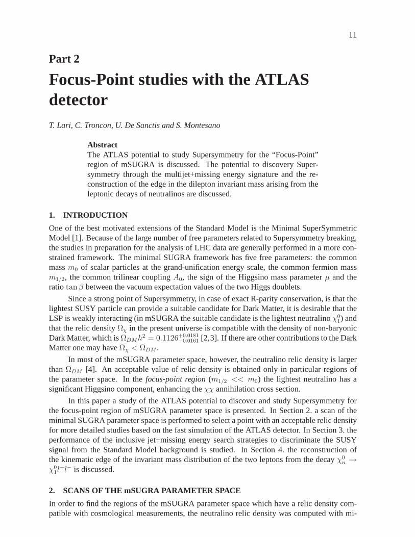
Figure 1: The picture shows the regions of the(m0,m1/2) mSUGRA plane which have a neutralino relic density

compatible with cosmological measurements in red/dark gray. The black region is excluded by LEP. The light

gray region has a neutralino relic density which exceeds cosmological constraints. White regions are theoretically

excluded. The values oftanβ = 10,A0 = 0, a positiveµ, and a top mass of 175 GeV were used.

In Fig. 1 a scan of the(m0, m1/2) plane is presented, for fixed values oftanβ = 10,A0 = 0, and positiveµ. A top mass of 175 GeV was used. The red/dark gray region on theleftis the stau coannihilation strip, while that on the right is the focus-point region withΩχ < ΩDM .

The latter is found at large value ofm0 > 3 TeV, hence the scalar particles are very heavy,near or beyond the sensitivity limit of LHC searches. Sincem1/2 << m0, the gaugino (charginoand neutralino) and gluino states are much lighter. The SUSYproduction cross section at theLHC is thus dominated by gaugino and gluino pair production.

The dependence of the position of the focus-point region on mSUGRA and StandardModel parameters (in particular, the top mass) and the uncertainties related to the aproximationsused by different RGE codes are discussed elsewhere [8–10].

Particle Mass (GeV) Particle Mass (GeV) Particle Mass (GeV)χ0

1 103.35 b1 2924.8 ντ 3532.3χ0

2 160.37 b2 3500.6 h 119.01χ0

3 179.76 t1 2131.1 H0 3529.7χ0

4 294.90 t2 2935.4 A0 3506.6χ±

1 149.42 eL 3547.5 H± 3530.6χ±

2 286.81 eR 3547.5g 856.59 νe 3546.3uL 3563.2 τ1 3519.6uR 3574.2 τ2 3533.7

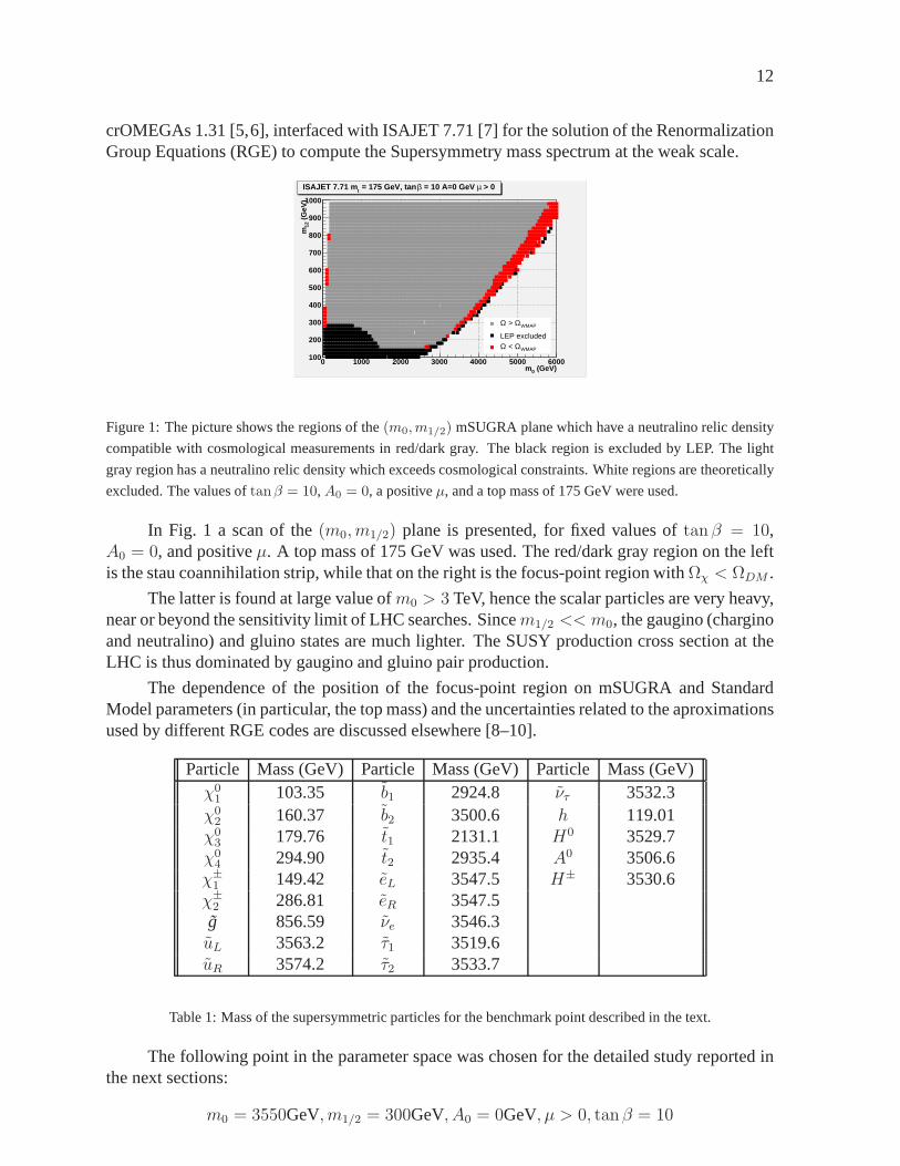
Table 1: Mass of the supersymmetric particles for the benchmark point described in the text.

The following point in the parameter space was chosen for thedetailed study reported inthe next sections:

m0 = 3550GeV, m1/2 = 300GeV, A0 = 0GeV, µ > 0, tanβ = 10

13

with the top mass set to 175 GeV and the mass spectrum computedwith ISAJET. In table 1the mass of SUSY particles for this point are reported. The scalar partners of Standard Modelfermions have a mass larger than 2 TeV. The neutralinos and charginos have masses between100 GeV and 300 GeV. The gluino is the lightest colored state,with a mass of 856.6 GeV. Thelightest Higgs boson has a mass of 119 GeV, while the other Higgs states have a mass wellbeyond the LHC reach at more than 3 TeV.

The total SUSY production cross section at the LHC, as computed by HERWIG [11–13],is 5.00 pb. It is dominated by the production of gaugino pairs, χ0χ0 (0.22 pb),χ0χ± (3.06 pb),andχ±χ± (1.14 pb).

The production of gluino pairs (0.58 pb) is also significant.The gluino decays intoχ0qq(29.3%),χ0g (6.4%), orχ±qq

′(54.3%). The quarks in the final state belongs to the third

generation in 75.6% of the decays.

The direct production of gaugino pairs is difficult to separate from the Standard Modelbackground; one possibility is to select events with several leptons, arising from the leptonicdecays of neutralinos and charginos.

The production of gluino pairs can be separated from the Standard Model by requiringthe presence of several high-pT jets and missing transverse energy. The presence ofb-jets andleptons from the top and gaugino decays can also be used.

In the analysis presented here, the event selection is basedon the multijet+missing energysignature. This strategy selects the events from gluino pair production, while rejecting both theStandard Model background and most of the gaugino direct production.

3. INCLUSIVE SEARCHES

The production of Supersymmetry events at the LHC was simulated using HERWIG 6.55 [11–13]. The top background was produced using MC@NLO 2.31 [14, 15]. The fully inclusivettproduction was simulated. This is expected to be the dominant Standard Model background forthe analysis presented in this note. The W+jets, and Z+jets background were produced usingPYTHIA 6.222 [16,17]. The vector bosons were forced to decayleptonically, and the transversemomentum of the W and the Z at generator level was required to be larger than 120 GeV and100 GeV, respectively.

The events were then processed by ATLFAST [18] to simulate the detector response.

The most abundant gluino decay modes areg → χ0tt and g → χ±tb. Events withgluino pair production have thus at least four hard jets, andmay have many more additional jetsbecause of the top hadronic decay modes and the chargino and neutralino decays. When bothgluinos decay to third generation quarks at least 4 jets areb-jets. A missing energy signature isprovided by the twoχ0

1 in the final state, and possibly by neutrinos coming from the top quarkand the gaugino leptonic decay modes.

The following selections were made to separate these eventsfrom the Standard Modelbackground:

• At least one jet withpT > 120 GeV• At least four jets withpT > 50 GeV, and at least two of them tagged asb-jets.• ET

MISS > 100 GeV• 0.1 < ET

MISS/MEFF < 0.35

• No isolated lepton (electron or muon) withpT > 20 GeV and|η| < 2.5.

14

Sample Events Basic cuts 2 b-jetsSUSY 50000 2515 1065tt 7600000 67089 11987

W+jets 3000000 16106 175Z+jets 1900000 6991 147

Table 2: Efficiency of the cuts used for the inclusive search,evaluated with ATLFAST events for low luminosity

operation. The number of events corresponds to an integrated luminosity of 10 fb−1. The third column reports

the number of events which passes the cuts described in the text, except the requirement of two b-jets, which is

reported in the last column.

Here, the effective massMEFF is defined as the scalar sum of the transverse missingenergy and the transverse momentum of all the reconstructedhadronic jets.

The efficiency of these cuts is reported in Tab. 2. The third column reports the number ofevents which passes the selections reported above, except the requirement of twob-jets, whichis added to obtain the numbers in the last column. The standard ATLAS b-tagging efficiency of60% for a rejection factor of 100 on light jets is assumed.

The SUSY events which pass the selection are almost exclusively due to gluino pair pro-duction; the gaugino direct production (about 90% of the total SUSY cross section) does notpass the cuts on jets and missing energy. After all selections the dominant background is by fardue tott production. The requirement of twob-jets supresses the remainingW+jets andZ+jetsbackgrounds by two orders of magnitude and is also expected to reduce the background fromQCD multi-jet production (which has not been simulated) to negligible levels.

Effective Mass (GeV)0 500 1000 1500 2000 2500 3000 3500 4000 4500 5000

Effective Mass (GeV)0 500 1000 1500 2000 2500 3000 3500 4000 4500 5000

/100

GeV

-1E

ven

ts/1

0 fb

1

10

210

310

410

Meff

SU2tt, MCatNLOZ+jets, PYTHIAW+jets, PYTHIA

Meff

Figure 2: Distribution of the effective mass defined in the text, for SUSY events and the Standard Model back-

grounds. The number of events correspond to an integrated luminosity of 10 fb−1.

The distribution of the effective mass after these selection cuts is reported in Fig. 2.The statistic corresponds to an integrated luminosity of 10fb−1. The signal/background ra-tio for an effective mass larger than 1500 GeV is close to 1 andthe statistical significance isSUSY/

√SM = 23.

15

Sample Events after cuts Mll < 80 GeVSUSY 50000 185 107tt 7600000 31 13

W+jets 3000000 0 0Z+jets 1200000 1 0

Table 3: Efficiency of the cuts used for the reconstruction ofthe neutralino leptonic decay. The number of events

corresponds to an integrated luminosity of 10 fb−1. The third column contains the number of events which passes

the selection cuts described in the text. The last column reports the number of the events passing the cuts which

have an invariant mass of the two leptons lower than 80 GeV.

4. THE DI-LEPTON EDGE

For the selected benchmark, the decays

χ02 → χ0

1l+l− (1)

χ03 → χ0

1l+l− (2)

occur with a branching ratio of 3.3% and 3.8% per lepton flavour respectively. The two leptonsin the final state provide a natural trigger and a clear signature. Their invariant mass has akinematic maximum equal to the mass difference of the two neutralinos involved in the decay,which is

mχ02−mχ0

1= 57.02 GeV mχ0

3−mχ0

1= 76.41 GeV (3)

The analysis of the simulated data was performed with the following selections:

• Two isolated leptons with opposite charge and same flavour with pT > 10 GeV and|η| < 2.5

• ETMISS > 80 GeV,MEFF > 1200 GeV,0.06 < ET

MISS/MEFF < 0.35

• At least one jet withpT > 80 GeV, at least four jets withpT > 60 GeV and at least sixjets withpT > 40 GeV

The efficiency of the various cuts is reported in table 3 for anintegrated statistics of10 fb−1. After all cuts, 107 SUSY and 13 Standard Model events are left with a 2-leptoninvariant mass smaller than 80 GeV. The dominant Standard Model background comes fromttproduction, and it is small compared to the SUSY combinatorial background: only half of theselected SUSY events do indeed have the decay (1) or (2) in theMontecarlo Truth record.

It should be noted that with these selections, the ratioSUSY/√SM is 30, which is

slightly larger than the significance provided by the selections of the inclusive search with leptonveto. The two lepton signature, with missing energy and hardjet selections is thus an excellentSUSY discovery channel.

The combinatorial background can be estimated from the datausing thee+µ− andµ+e−

pairs. In the leftmost plot of Fig. 3 the distribution of the lepton invariant mass is reported forSUSY events with the same (different) flavour as yellow (red)histograms. Outside the signalregion and the Z peak the two histograms are compatible. The Standard Model distribution is

16

(GeV)invM0 20 40 60 80 100 120 140 160 180

Eve

nts

-5

0

5

10

15

20

)tleptons same flavour (t

)tleptons different flavour (t0.28)×, χ∼leptons same flavour (

0.28)×, χ∼leptons different flavour (

/ ndf 2χ 38.5 / 35Prob 0.3143p0 7.56± 53.89 p1 6.61± 43.63 p2 91.87± -74.51 p3 0.49± -56.99 p4 1.15± 77.27

(GeV)invM0 20 40 60 80 100 120

Eve

nts

0

50

100

150

200

/ ndf 2χ 38.5 / 35Prob 0.3143p0 7.56± 53.89 p1 6.61± 43.63 p2 91.87± -74.51 p3 0.49± -56.99 p4 1.15± 77.27

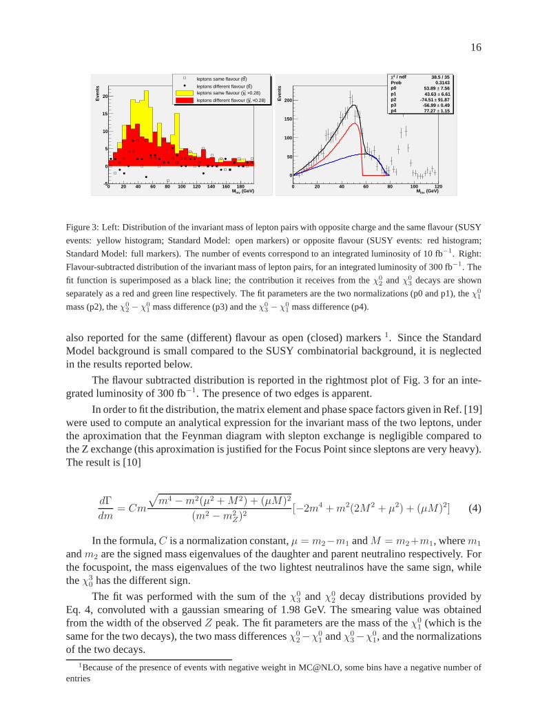
Figure 3: Left: Distribution of the invariant mass of leptonpairs with opposite charge and the same flavour (SUSY

events: yellow histogram; Standard Model: open markers) oropposite flavour (SUSY events: red histogram;

Standard Model: full markers). The number of events correspond to an integrated luminosity of 10 fb−1. Right:

Flavour-subtracted distribution of the invariant mass of lepton pairs, for an integrated luminosity of 300 fb−1. The

fit function is superimposed as a black line; the contribution it receives from theχ02 andχ0

3 decays are shown

separately as a red and green line respectively. The fit parameters are the two normalizations (p0 and p1), theχ01

mass (p2), theχ02 − χ0

1 mass difference (p3) and theχ03 − χ0

1 mass difference (p4).

also reported for the same (different) flavour as open (closed) markers1. Since the StandardModel background is small compared to the SUSY combinatorial background, it is neglectedin the results reported below.

The flavour subtracted distribution is reported in the rightmost plot of Fig. 3 for an inte-grated luminosity of 300 fb−1. The presence of two edges is apparent.

In order to fit the distribution, the matrix element and phasespace factors given in Ref. [19]were used to compute an analytical expression for the invariant mass of the two leptons, underthe aproximation that the Feynman diagram with slepton exchange is negligible compared tothe Z exchange (this aproximation is justified for the Focus Point since sleptons are very heavy).The result is [10]

dΓ

dm= Cm

√

m4 −m2(µ2 +M2) + (µM)2

(m2 −m2Z)2

[−2m4 +m2(2M2 + µ2) + (µM)2] (4)

In the formula,C is a normalization constant,µ = m2−m1 andM = m2+m1, wherem1

andm2 are the signed mass eigenvalues of the daughter and parent neutralino respectively. Forthe focuspoint, the mass eigenvalues of the two lightest neutralinos have the same sign, whiletheχ3

0 has the different sign.

The fit was performed with the sum of theχ03 andχ0

2 decay distributions provided byEq. 4, convoluted with a gaussian smearing of 1.98 GeV. The smearing value was obtainedfrom the width of the observedZ peak. The fit parameters are the mass of theχ0

1 (which is thesame for the two decays), the two mass differencesχ0

2−χ01 andχ0

3−χ01, and the normalizations

of the two decays.1Because of the presence of events with negative weight in MC@NLO, some bins have a negative number of

entries

17

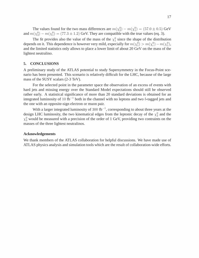
The values found for the two mass differences arem(χ02) −m(χ0

1) = (57.0 ± 0.5) GeVandm(χ0

3) −m(χ01) = (77.3 ± 1.2) GeV. They are compatible with the true values (eq. 3).

The fit provides also the value of the mass of theχ01 since the shape of the distribution

depends on it. This dependence is however very mild, expecially for m(χ01) > m(χ0

i )−m(χ01),

and the limited statistics only allows to place a lower limitof about 20 GeV on the mass of thelightest neutralino.

5. CONCLUSIONS

A preliminary study of the ATLAS potential to study Supersymmetry in the Focus-Point sce-nario has been presented. This scenario is relatively difficult for the LHC, because of the largemass of the SUSY scalars (2-3 TeV).

For the selected point in the parameter space the observation of an excess of events withhard jets and missing energy over the Standard Model expectations should still be observedrather early. A statistical significance of more than 20 standard deviations is obtained for anintegrated luminosity of10 fb−1 both in the channel with no leptons and twob-tagged jets andthe one with an opposite-sign electron or muon pair.

With a larger integrated luminosity of300 fb−1, corresponding to about three years at thedesign LHC luminosity, the two kinematical edges from the leptonic decay of theχ0

2 and theχ0

3 would be measured with a precision of the order of 1 GeV, providing two contraints on themasses of the three lightest neutralinos.

Acknowledgements

We thank members of the ATLAS collaboration for helpful discussions. We have made use ofATLAS physics analysis and simulation tools which are the result of collaboration-wide efforts.

18

Part 3

SUSY parameter determination in thechallenging focus point-inspired caseK. Desch, J. Kalinowski, G. Moortgat-Pick and K. Rolbiecki

AbstractInspired by focus point scenarios we discuss the potential of combinedLHC and ILC experiments for SUSY searches in a difficult region ofthe parameter space in which all sfermions are above the TeV.Precisionanalyses of cross sections of light chargino production andforward-backward asymmetries of decay leptons at the ILC together with massinformation onmχ0

2from the LHC allow to fit rather precisely the un-

derlying fundamental gaugino/higgsino MSSM parameters and to con-strain the masses of the heavy, kinematically not accessible, virtualsparticles. For such analyses the complete spin correlations betweenproduction and decay process have to be taken into account. We alsotook into account expected experimental uncertainties.

1. INTRODUCTION

Due to the unknown mechanism of SUSY breaking, supersymmetric extensions of the Stan-dard Model contain a large number of new parameters: 105 in the Minimal SupersymmetricStandard Model (MSSM) appear and have to be specified. Experiments at future accelerators,the LHC and the ILC, will have not only to discover SUSY but also to determine precisely theunderlying scenario without theoretical prejudices on theSUSY breaking mechanism. Particu-larly challenging are scenarios, where the scalar SUSY particle sector is heavy, as required e.g.in focus point scenarios (FP) as well as in split SUSY (sS). For a recent study of a mSUGRAFP scenario at the LHC, see [20].

Many methods have been worked out how to derive the SUSY parameters at colliderexperiments [21, 22]. In [23–27] the chargino and neutralino sectors have been exploited todetermine the MSSM parameters. However, in most cases only the production processes havebeen studied and, furthermore, it has been assumed that the masses of scalar particles are alreadyknown. In [28] a fit has been applied to the chargino production in order to deriveM2, µ, tan βandmνe . However, in the case of heavy scalars such fits lead to a rather weak constraint formνe .

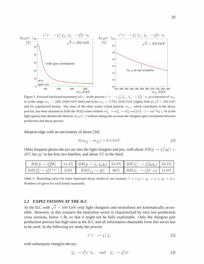
Since it is not easy to determine experimentally cross sections for production processes,studies have been made to exploit the whole production-and-decay process. Angular and energydistributions of the decay products in production with subsequent three-body decays have beenstudied for chargino as well as neutralino processes in [29–31]. Since such observables dependstrongly on the polarization of the decaying particle the complete spin correlations betweenproduction and decay can have large influence and have to be taken into account: Fig. 1 showsthe effect of spin correlation on the forward-backward asymmetry as a function of sneutrinomass in the scenario considered below. Exploiting such spineffects, it has been shown in [32,

19

33] that, once the chargino parameters are known, useful indirect bounds for the mass of theheavy virtual particles could be derived from forward-backward asymmetries of the final leptonAFB(ℓ).

2. CHOSEN SCENARIO: FOCUS POINT-INSPIRED CASE

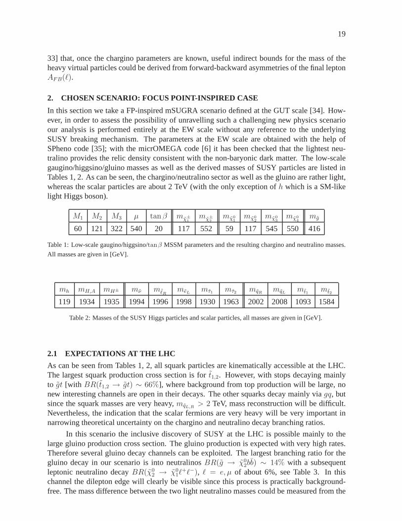
In this section we take a FP-inspired mSUGRA scenario definedat the GUT scale [34]. How-ever, in order to assess the possibility of unravelling sucha challenging new physics scenarioour analysis is performed entirely at the EW scale without any reference to the underlyingSUSY breaking mechanism. The parameters at the EW scale are obtained with the help ofSPheno code [35]; with the micrOMEGA code [6] it has been checked that the lightest neu-tralino provides the relic density consistent with the non-baryonic dark matter. The low-scalegaugino/higgsino/gluino masses as well as the derived masses of SUSY particles are listed inTables 1, 2. As can be seen, the chargino/neutralino sector as well as the gluino are rather light,whereas the scalar particles are about 2 TeV (with the only exception ofh which is a SM-likelight Higgs boson).

M1 M2 M3 µ tanβ mχ±1

mχ±2

mχ01

mχ02

mχ03

mχ04

mg

60 121 322 540 20 117 552 59 117 545 550 416

Table 1: Low-scale gaugino/higgsino/tanβ MSSM parameters and the resulting chargino and neutralino masses.

All masses are given in [GeV].

mh mH,A mH± mν mℓRmeL

mτ1 mτ2 mqR mqL mt1 mt2

119 1934 1935 1994 1996 1998 1930 1963 2002 2008 1093 1584

Table 2: Masses of the SUSY Higgs particles and scalar particles, all masses are given in [GeV].

2.1 EXPECTATIONS AT THE LHC

As can be seen from Tables 1, 2, all squark particles are kinematically accessible at the LHC.The largest squark production cross section is fort1,2. However, with stops decaying mainlyto gt [with BR(t1,2 → gt) ∼ 66%], where background from top production will be large, nonew interesting channels are open in their decays. The othersquarks decay mainly viagq, butsince the squark masses are very heavy,mqL,R

> 2 TeV, mass reconstruction will be difficult.Nevertheless, the indication that the scalar fermions are very heavy will be very important innarrowing theoretical uncertainty on the chargino and neutralino decay branching ratios.

In this scenario the inclusive discovery of SUSY at the LHC ispossible mainly to thelarge gluino production cross section. The gluino production is expected with very high rates.Therefore several gluino decay channels can be exploited. The largest branching ratio for thegluino decay in our scenario is into neutralinosBR(g → χ0

2bb) ∼ 14% with a subsequentleptonic neutralino decayBR(χ0

2 → χ01ℓ

+ℓ−), ℓ = e, µ of about 6%, see Table 3. In thischannel the dilepton edge will clearly be visible since thisprocess is practically background-free. The mass difference between the two light neutralino masses could be measured from the

20

e+e− → χ+1 χ

−1 , χ−

1 → χ01e

−νeAFB(e−)

[%]

mνe /GeV

√s = 350 GeV

with spin correlations

w/ospin cor.

0

10

20

30

40

50

60

500 1000 1500 2000 3.8

4.0

4.2

4.4

4.6

4.8

5.0

5.2

1750 1800 1850 1900 1950 2000 2050 2100 2150 2200 2250

AFB in our scenario↑

AFB(e−)

[%]

mνe /GeV

√s = 350 GeV

e+e− → χ+1 χ

−1 , χ−

1 → χ01e

−νe

Figure 1: Forward-backward asymmetry ofe− in the processe+e− → χ+1 χ

−

1 , χ−

1 → χ01e

−νe as a function ofmνe

in a) the rangemνe= [200, 2300] GeV (left) and in b)mνe

= [1750, 2250] GeV (right), both at√s = 350 GeV

and for unpolarized beams. The mass of the other scalar virtual particle,meL, which contributes in the decay

process, has been assumed to fulfil the SU(2) mass relationm2eL

= m2νe

+m2Z cos(2β)(−1 + sin2 θW ). In a) the

light (green) line denotes the derivedAFB(e−) without taking into account the chargino spin correlationsbetween

production and decay process.

dilepton edge with an uncertainty of about [34]

δ(mχ02−mχ0

1) ∼ 0.5 GeV. (1)

Other frequent gluino decays are into the light chargino andjets, with aboutBR(g → χ±1 qq

′) ∼20% for qq′ in the first two families, and about3% in the third.

BR(g → χ02bb) 14.4% BR(g → χ−

1 quqd) 10.8% BR(χ+1 → χ0

1qdqu) 33.5%

BR(χ02 → χ0

1ℓ+ℓ−) 3.0% BR(t1,2 → gt) 66% BR(χ−

1 → χ01ℓ

−νℓ) 11.0%

Table 3: Branching ratios for some important decay modes in our scenario,ℓ = e, µ, τ , qu = u, c, qd = d, s.

Numbers are given for each family separately.

2.2 EXPECTATIONS AT THE ILC

At the ILC with√s = 500 GeV only light charginos and neutralinos are kinematicallyacces-

sible. However, in this scenario the neutralino sector is characterized by very low productioncross sections, below 1 fb, so that it might not be fully exploitable. Only the chargino pairproduction process has high rates at the ILC and all information obtainable from this sector hasto be used. In the following we study the process

e+e− → χ+1 χ

−1 (2)

with subsequent chargino decays

χ−1 → χ0

1e−νe, and χ−

1 → χ01sc (3)

21

for which the analytical formulae including the complete spin correlations are given in a com-pact form e. g. in [29]. The production process occurs viaγ andZ exchange in thes-channelandνe exchange in thet-channel, and the decay processes get contributions fromW±-exchangeandνe, eL (leptonic decays) orsL, cL (hadronic decays).

Table 4 lists the chargino production cross sections and forward-backward asymmetriesfor different beam polarization configurations and the1σ statistical uncertainty based onL =200 fb−1 for each polarization configuration,(Pe−, Pe+) = (−90%,+60%) and(+90%,−60%).Below we constrain our analyses to the first step of the ILC with

√s ≤ 500 GeV and study only

theχ+1 χ

−1 production and decay.

Studies of chargino production with semi-leptonic decays at the ILC runs at√s = 350

and500 GeV will allow to measure the light chargino mass in the continuum with an error∼ 0.5 GeV. This can serve to optimize the ILC scan at the threshold [36] which, due to thesteeps-wave excitation curve inχ+

1 χ−1 production, can be used to determine the light chargino

mass very precisely to about [37–39]

mχ±1

= 117.1 ± 0.1 GeV. (4)

The light chargino has a leptonic branching ratio of aboutBR(χ−1 → χ0

1ℓ−νℓ) ∼ 11% for

each family and a hadronic branching ratio of aboutBR(χ−1 → χ0

1sc) ∼ 33%. The mass of thelightest neutralinomχ0

1can be derived either from the energy distribution of the lepton ℓ− or in

hadronic decays from the invariant mass distribution of thetwo jets. We therefore assume [34]

mχ01

= 59.2 ± 0.2 GeV. (5)

Together with the information from the LHC, Eq. (1), a mass uncertainty for the second lightestneutralino of about

mχ02

= 117.1 ± 0.5 GeV. (6)

can be assumed.

3. PARAMETER DETERMINATION

3.1 Parameter fit without using the forward-backward asymmetry

In the fit we use polarized chargino cross section multipliedby the branching ratios of semi-leptonic chargino decays:σ(e+e− → χ+

1 χ−1 ) × BR, with BR = 2 × BR(χ+

1 → χ01qdqu) ×

BR(χ−1 → χ0

1ℓ−ν) + [BR(χ−

1 → χ01ℓ

−ν)]2 ∼ 0.34, ℓ = e, µ, qu = u, c, qd = d, s, as givenin Table 4. We take into account1σ statistical error, a relative uncertainty in polarizationof∆Pe±/Pe± = 0.5% [40] and an experimental efficiency of 50%,cf. Table 4.

We applied a four-parameter fit for the parametersM1, M2, µ andmνe for fixed tan β =5,10,15,20,25,30 values. Fixingtanβ was necessary for a proper convergence of the minimal-ization procedure. For the input valuetanβ = 20 we obtain

M1 = 60.0±0.2 GeV, M2 = 121.0±0.7 GeV, µ = 540±50 GeV, mνe = 2000±100 GeV.(7)

Due to the strong gaugino component ofχ±1 andχ0

1,2, the parametersM1 andM2 are welldetermined with a relative uncertainty of∼ 0.5%. The higgsino parameterµ as well asmνe aredetermined to a lesser degree, with relative errors of∼ 10% and 5%. Note however, that theerrors, as well as the fitted central values depend ontan β. Figure 2 shows the migration of 1σ

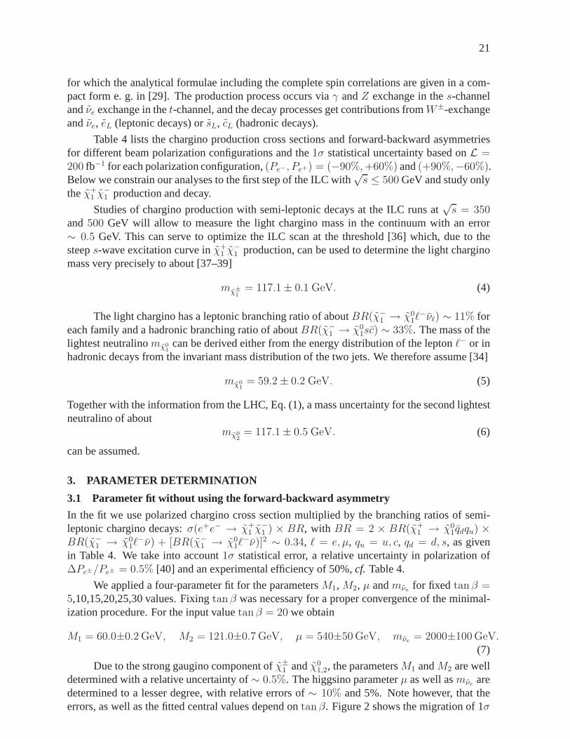
22

M2

mνe

µ

M2

M2

M1

Figure 2: Migration of 1σ contours withtanβ = 5, 10, 20, 30 (top-to-bottom in the left panel, right-to-left in the

middle panel, top-to-bottom in the right panel).

contours inmνe–M2 (left), M2–µ (middle) andM1–M2 (right) panels. Varyingtan β between5 and 30 leads to a shift∼ 1 GeV of the fittedM1 value and∼ 3.5 GeV ofM2, increasingeffectively their experimental errors, while the migration effect forµ andmνe is much weaker.

3.2 Parameter fit including the forward-backward asymmetry

Following the method proposed in [32, 33] we now extend the fitby using as additional ob-servable the forward-backward asymmetry of the final electron. As explained in the sectionsbefore, this observable is very sensitive to the mass of the exchanged scalar particles, evenfor rather heavy masses, see Fig. 1 (right). Since in the decay process also the left selec-tron exchange contributes theSU(2) relation between the left selectron and sneutrino masses:m2eL

= m2νe

+m2Z cos(2β)(−1 + sin2 θW ) has been assumed [21]. In principle this assumption

could be tested by combing the leptonic forward-backward asymmetry with that in the hadronicdecay channels if the squark masses could be measured at the LHC [34].

We take into account a1σ statistical uncertainty for the asymmetry which is given by

∆(AFB) = 2√

ǫ(1 − ǫ)/N, (8)

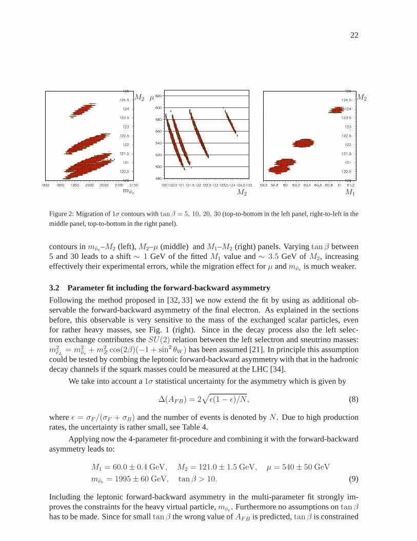
whereǫ = σF/(σF + σB) and the number of events is denoted byN . Due to high productionrates, the uncertainty is rather small, see Table 4.

Applying now the 4-parameter fit-procedure and combining itwith the forward-backwardasymmetry leads to:

M1 = 60.0 ± 0.4 GeV, M2 = 121.0 ± 1.5 GeV, µ = 540 ± 50 GeV

mνe = 1995 ± 60 GeV, tan β > 10. (9)

Including the leptonic forward-backward asymmetry in the multi-parameter fit strongly im-proves the constraints for the heavy virtual particle,mνe. Furthermore no assumptions ontan βhas to be made. Since for smalltanβ the wrong value ofAFB is predicted,tan β is constrained

23

√s/GeV (Pe−, Pe+) σ(χ+

1 χ−1 )/fb σ(χ+

1 χ−1 ) × BR/fb AFB(e−)/%

350 (−90%,+60%) 6195.5±7.9 2127.9±4.0 4.49±0.32

(0, 0) 2039.1±4.5 700.3±2.7 4.5±0.5

(+90%,−60%) 85.0±0.9 29.2±0.7 4.7±2.7

500 (−90%,+60%) 3041.5±5.5 1044.6±2.3 4.69±0.45

(0, 0) 1000.6±3.2 343.7±1.7 4.7±0.8

(+90%,−60%) 40.3±0.4 13.8±0.4 5.0±3.9

Table 4: Cross sections for the processe+e− → χ+1 χ

−

1 and forward-backward asymmetries for this process

followed by χ−

1 → χ01e

−νe, for different beam polarizationPe− , Pe+ configurations at the cm energies√s =

350 GeV and500 GeV at the ILC. Errors include1σ statistical uncertainty assumingL = 200 fb−1 for each

polarization configuration, and beam polarization uncertainty of 0.5%.BR ≃ 0.34, cf. Sec. 3.1 and Table 3.

from below. The constraints for the massmνe are improved by about a factor 2 and for gauginomass parametersM1 andM2 by a factor 3, as compared to the results of the previous sectionwith unconstrainedtan β. The error for the higgsino mass parameterµ remains roughly thesame. It is clear that in order to improve considerably the constraints for the parameterµ themeasurement of the heavy higgsino-like chargino and/or neutralino masses will be necessary atthe second phase of the ILC with

√s ∼ 1000 GeV.

4. CONCLUSIONS

In [34] we show the method for constraining heavy virtual particles and for determining theSUSY parameters in focus-point inspired scenarios. Such scenarios appear very challengingsince there is only a little experimental information aboutthe SUSY sector accessible. How-ever, we show that a careful exploitation of data leads to significant constraints for unknown pa-rameters. The most powerful tool in this kind of analysis turns out to be the forward-backwardasymmetry. The proper treatment of spin correlations between the production and the decay is amust in that context. This asymmetry is strongly dependent on the mass of the exchanged heavyparticle. TheSU(2) assumption on the left selectron and sneutrino masses couldbe tested bycombing the leptonic forward-backward asymmetry with the forward-backward asymmetry inthe hadronic decay channels if the squark masses could be measured at the LHC [34]. Wewant to stress the important role of the LHC/ILC interplay since none of these colliders alonecan provide us with data needed to perform the SUSY parameterdetermination in focus-likescenarios.

Acknowledgements

The authors would like to thank the organizers of Les Houches2005 for the kind invitation andthe pleasant atmosphere at the workshop. This work is supported by the European Community’sHuman Potential Programme under contract HPRN-CT-2000-00149 and by the Polish StateCommittee for Scientific Research Grant No 2 P03B 040 24.

24

Part 4

mSUGRA validity of the Barr neutralinospin analysis at the LHCB.C. Allanach and F. Mahmoudi

AbstractThe Barr spin analysis allows the discrimination of supersymmetric spinassignments from other possibilities by measuring a chargeasymmetryat the LHC. The possibility of such a charge asymmetry relieson asquark-anti squark production asymmetry. We study the approximateregion of validity of such analyses in mSUGRA parameter space byestimating where the production asymmetry may be statistically signif-icant.

If signals consistent with supersymmetry (SUSY) are discovered at the LHC, it will bedesirable to check the spins of SUSY particles in order to test the SUSY hypothesis directly.There is the possibility, for instance, of producing a similar spectrum of particles as the minimalsupersymmetric standard model (MSSM) in the universal extra dimensions (UED) model [41].In UED, the first Kaluza-Klein modes of Standard Model particles have similar couplings totheir MSSM analogues, but their spins differ by1/2.

In a recent publication [42], Barr proposed a method to determine the spin of supersym-metric particles at the LHC from studying theq → χ0

2 q → lR ln q → χ01lnlf q decay chain.

Depending upon the charges of the various sparticles involved, the near and far leptons (ln, lfrespectively) may have different charges. Forming the invariant mass ofln with the quark nor-malised to its maximum value:m ≡ mlnq/m

maxlnq

= sin(θ∗/2), whereθ∗ is the angle betweenthe quark and near lepton in theχ0

2 rest frame. Barr’s central observation is that the probabilitydistribution functionP1 for l+n q or l−n q is different toP2 (the probability distribution function ofl−n q or l+n q) due to different helicity factors:

dP1

dm= 4m3,

dP2

dm= 4m(1 − m2). (1)

One cannot in practice distinguishq (originating from a squark) fromq (originating from ananti-squark), but insteadaveragesthe q, q distributions by simply measuring a jet. This summay therefore be distinguished against the pure phase-space distribution

dPPSdm

= 2m (2)

only if the expected number of produced squarks is differentto the number of anti-squarks2.Indeed, the distinguishing power of the spin measurement isproportional to the squark-antisquark production asymmetry. The relevant production processes arepp → q ˜q, gq or g ˜q. Thelatter two processes may have different cross-sections because of the presence of valence quarks

2One also cannot distinguish between near and far leptons, and so one must forml+q andl−q distributions [42].

25

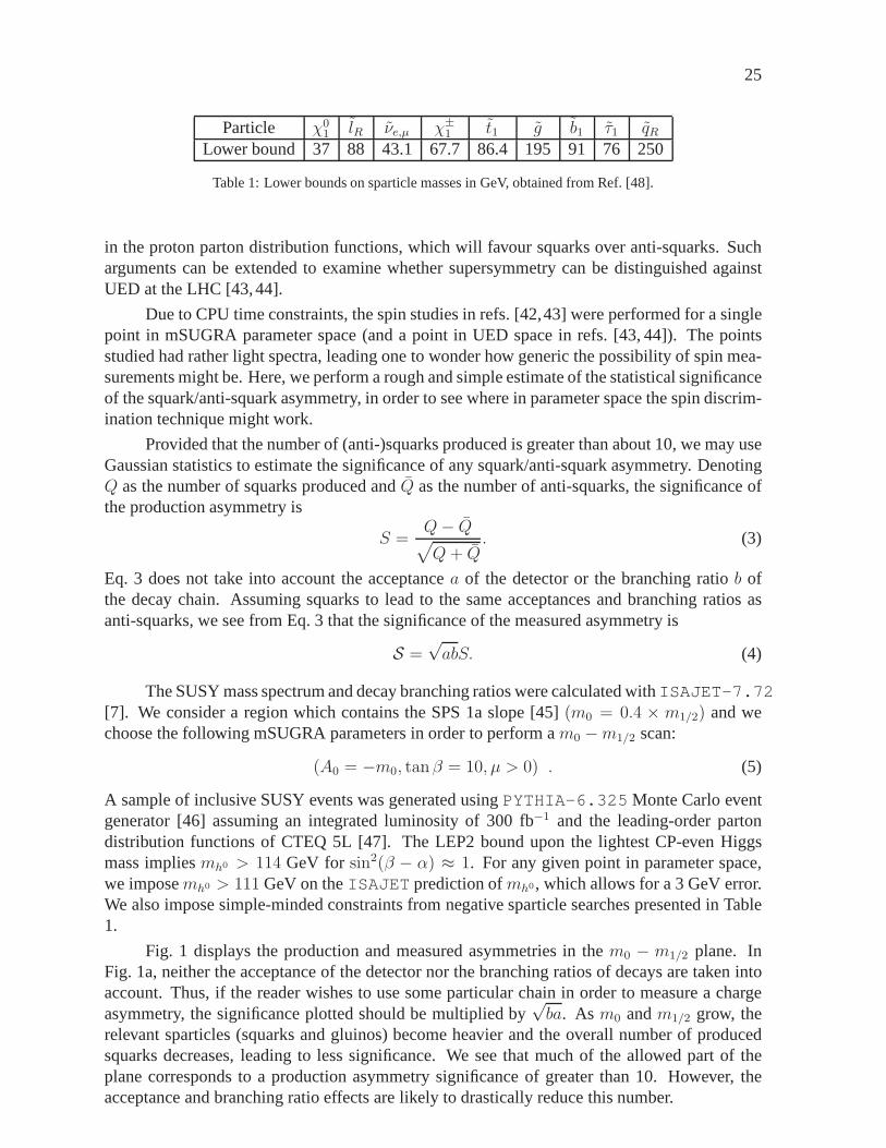
Particle χ01 lR νe,µ χ±

1 t1 g b1 τ1 qRLower bound 37 88 43.1 67.7 86.4 195 91 76 250

Table 1: Lower bounds on sparticle masses in GeV, obtained from Ref. [48].

in the proton parton distribution functions, which will favour squarks over anti-squarks. Sucharguments can be extended to examine whether supersymmetrycan be distinguished againstUED at the LHC [43,44].

Due to CPU time constraints, the spin studies in refs. [42,43] were performed for a singlepoint in mSUGRA parameter space (and a point in UED space in refs. [43, 44]). The pointsstudied had rather light spectra, leading one to wonder how generic the possibility of spin mea-surements might be. Here, we perform a rough and simple estimate of the statistical significanceof the squark/anti-squark asymmetry, in order to see where in parameter space the spin discrim-ination technique might work.

Provided that the number of (anti-)squarks produced is greater than about 10, we may useGaussian statistics to estimate the significance of any squark/anti-squark asymmetry. DenotingQ as the number of squarks produced andQ as the number of anti-squarks, the significance ofthe production asymmetry is

S =Q− Q√

Q+ Q. (3)

Eq. 3 does not take into account the acceptancea of the detector or the branching ratiob ofthe decay chain. Assuming squarks to lead to the same acceptances and branching ratios asanti-squarks, we see from Eq. 3 that the significance of the measured asymmetry is

S =√abS. (4)

The SUSY mass spectrum and decay branching ratios were calculated withISAJET-7.72[7]. We consider a region which contains the SPS 1a slope [45](m0 = 0.4 × m1/2) and wechoose the following mSUGRA parameters in order to perform am0 −m1/2 scan:

(A0 = −m0, tanβ = 10, µ > 0) . (5)

A sample of inclusive SUSY events was generated usingPYTHIA-6.325 Monte Carlo eventgenerator [46] assuming an integrated luminosity of 300 fb−1 and the leading-order partondistribution functions of CTEQ 5L [47]. The LEP2 bound upon the lightest CP-even Higgsmass impliesmh0 > 114 GeV for sin2(β − α) ≈ 1. For any given point in parameter space,we imposemh0 > 111 GeV on theISAJET prediction ofmh0, which allows for a 3 GeV error.We also impose simple-minded constraints from negative sparticle searches presented in Table1.

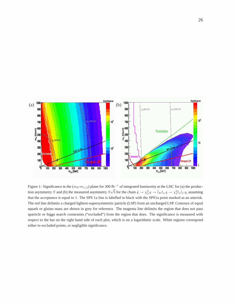
Fig. 1 displays the production and measured asymmetries in them0 − m1/2 plane. InFig. 1a, neither the acceptance of the detector nor the branching ratios of decays are taken intoaccount. Thus, if the reader wishes to use some particular chain in order to measure a chargeasymmetry, the significance plotted should be multiplied by

√ba. As m0 andm1/2 grow, the

relevant sparticles (squarks and gluinos) become heavier and the overall number of producedsquarks decreases, leading to less significance. We see thatmuch of the allowed part of theplane corresponds to a production asymmetry significance ofgreater than 10. However, theacceptance and branching ratio effects are likely to drastically reduce this number.

26

(a) (b)

Figure 1: Significance in the (m0-m1/2) plane for 300 fb−1 of integrated luminosity at the LHC for (a) the produc-

tion asymmetryS and (b) the measured asymmetryS√b for the chainq → χ0

2 q → lR ln q → χ01lnlf q, assuming

that the acceptance is equal to 1. The SPS 1a line is labelled in black with the SPS1a point marked as an asterisk.

The red line delimits a charged lightest-supersymmetric particle (LSP) from an uncharged LSP. Contours of equal

squark or gluino mass are shown in grey for reference. The magenta line delimits the region that does not pass

sparticle or higgs search constraints (“excluded”) from the region that does. The significance is measured with

respect to the bar on the right hand side of each plot, which ison a logarithmic scale. White regions correspond

either to excluded points, or negligible significance.

27

Fig. 1b includes the effect of the branching ratio for the chain that Barr studied in thesignificance. The significance is drastically reduced from Fig. 1a due to the small branchingratios involved. The region marked “charged LSP” is cosmologically disfavoured if the LSPis stable, but might be viable if R-parity is violated. In this latter case though, a different spinanalysis would have to be performed due to the presence of theLSP decay products. The regionmarked “forbidden” occurs whenmlR

> mχ02, implying that the decay chain studied by Barr

does not occur.

The highest squark/anti-squark asymmetry can be found aroundm0 = 100, m1/2 = 200and its significance is around 500 or so, including branchingratios. Barr investigated themSUGRA pointm0 = 100 GeV ,m1/2 = 300 GeV,A0 = m1/2, tanβ = 2.1, µ > 0, as-suming a luminosity of 500 fb−1. In his paper, which includes acceptance effects, Barr statesthat a significant spin measurement at this point should still be possible even with only 150 fb−1

of integrated luminosity. Our calculation of the significanceS√b for this point is 53. Assum-

ing that the acceptance is not dependent upon the mSUGRA parameters, we may deduce thata value ofS

√b > 53 in Fig. 1b is also viable with 150 fb−1. This roughly corresponds to the

orange and red regions in Fig. 1b. Although the parameter space is highly constrained, there isnevertheless a non-negligible region where the Barr spin analysis may work.

Acknowledgements

FM would like to thank Steve Muanza for his help regarding Pythia, and acknowledges thesupport of the McCain Fellowship at Mount Allison University. BCA thanks the CambrigeSUSY working group for suggestions. This work has been partially supported by PPARC.

28

Part 5

The trilepton signal in the focus pointregionPh. Gris, R. Lafaye, T. Plehn, L. Serin, L. Tompkins and D. Zerwas

AbstractWe examine the potential for a measurement of supersymmetryat theTevatron and at the LHC in the focus point region. In particular, westudy on the tri-lepton signal. We show to what precision supersym-metric parameters can be determined using measurements in the Higgssector as well as the mass differences between the two lightest neutrali-nos and between the gluino and the second-lightest neutralino.

1. INTRODUCTION

Recent high energy gamma ray observations from EGRET show anexcess of galactic gammarays in the 1 GeV range [49]. A possible explanation of the excess are photons generated byneutralino annihilation in galactic dark matter [50]. Unfortunately, this kind cosmological datais only sensitive to a few supersymmetric parameters, like the mass and the annihilation or de-tection cross sections of the weakly interacting dark matter candidate. A prime dark mattercandidate is the lightest supersymmetric particle, which in most supersymmetry breaking sce-narios turns out to be the lightest neutralino [51]. To be able to derive stronger statements fromthe data, one can assume gravity mediated supersymmetry breaking (mSUGRA) and fit the freeparameters of this constrained model to the observed gamma ray spectrum [50]. Only an addi-tional connection of this kind (assuming we know the supersymmetry breaking scenario) allowsone to make statements about the scalar sector. In this briefletter, we study the mSUGRA pa-rameter point given bym0 = 1400 GeV,m1/2 = 180 GeV,A0 = 700 GeV, tan β = 51 andµ > 0, which could explain the claimed excess. We analyse the phenomenological implicationsfor searches and measurements of supersymmetric particlesat the Tevatron and at the LHC [52].To determine the underlying mSUGRA parameters sophisticated tools such as Fittino [53, 54]and SFITTER [55, 56] are required. In our study we use SFITTERto determine the expectederrors on the supersymmetric parameters.

The TeV-scale particle masses for our mSUGRA parameter point are displayed in Ta-ble 1. The highm0 value [57–59] places most squarks and sleptons well above 1 TeV, whichmeans that the expected production rate at the LHC will be strongly reduced as compared to thestandard scenarios such as SPS1a [45]. The large value fortanβ enhances the heavy HiggsYukawa coupling tob quarks andτ leptons. Therefore the MSSM Higgs sector is likely to beobserved at the LHC, for example through a charged Higgs boson decaying toτ leptons [60,61]or through a precision mass measurement for the heavy neutral Higgs bosons decaying to muonpairs [52]. Certainly, the comparably low-mass charginos,neutralinos and gluinos, will be pro-duced at accelerator experiments.

29

Particle Mass (GeV) Particle Mass (GeV) Particle Mass (GeV)q 1430 g 520 h0 114b 974 χ±

1 137 A0 488l 1400 χ0

1 72τ 974 χ0

2 137

Table 1: TeV-scale supersymmetric particle masses in the EGRET parameter point computed with SUSPECT [62].

Figure 1: Tevatron reach in the trilepton channel in them0 − m1/2 plane, for fixed values ofA0, µ > 0 and

tanβ = 5, 35. We show results for 2, 10 and 30fb−1 total integrated luminosity. The figure is taken out of

Ref. [67]

2. DISCOVERY PROSPECTS

At the Run II of the Tevatron, the 500 GeV gluinos are unlikelyto be observed, in particular inthe limit of heavy squarks, because the powerful squark–gluino associated production channeldoes not contribute to the gluino rate. Only the light gauginosχ±

1 , χ01 , χ0

2 might be observable.One of the most promising channels for SUSY discovery at the Tevatron is the production ofa neutralino and a chargino with a subsequent decay to tri-leptons [63–67]:pp → χ±

1 χ02 →

3ℓ + ET + X. Unfortunately, for our SUSY parameter point, its rate strongly auppressed bythe heavy sleptons: the leading order cross section is onlyσ × BR ≃ 10 fb, with mild next-to-leading order corrections [68]. Depending on the luminosity delivered by the Tevatron [69],between 40 and 80 events are expected per experiment runninguntil 2009. Since the 67 GeVmass difference between theχ0

1 and theχ02 andχ±

1 is sizeable, the transverse momentum of thedecay leptons is large. At the generator level, thepT distribution of the leading (next-to-leading)lepton peaks around 35 GeV (25 GeV). Hence, given a large enough ratem triggering on thissignal will not be a problem. However, the cross-section is too low to allow a discovery: inFigure 1 [67] we see that an integrated luminosity of at least20 fb−1 is required to claim a 5σdiscovery.

At the LHC, the total inclusive SUSY particles production cross section for our parameterpoint is 19.8 pb. The largest contributions come from the processesgg → gg (50%), qq′ →χ0

2χ±1 (20%), andqq → χ±

1 χ∓1 (10%). The dominant source of SUSY particle production with

a decay to hard jets are of course gluino decays. We can extract the tri-lepton signal [70–73]

30

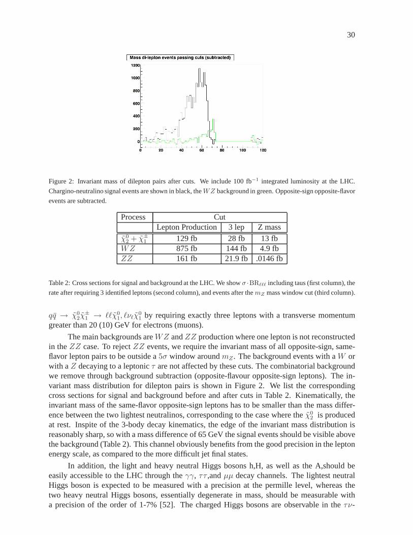
Figure 2: Invariant mass of dilepton pairs after cuts. We include 100 fb−1 integrated luminosity at the LHC.

Chargino-neutralino signal events are shown in black, theWZ background in green. Opposite-sign opposite-flavor

events are subtracted.

Process CutLepton Production 3 lep Z mass

χ02 + χ±

1 129 fb 28 fb 13 fbWZ 875 fb 144 fb 4.9 fbZZ 161 fb 21.9 fb .0146 fb

Table 2: Cross sections for signal and background at the LHC.We showσ ·BRℓℓℓ including taus (first column), the

rate after requiring 3 identified leptons (second column), and events after themZ mass window cut (third column).

qq → χ02χ

±1 → ℓℓχ0

1, ℓνℓχ01 by requiring exactly three leptons with a transverse momentum

greater than 20 (10) GeV for electrons (muons).

The main backgrounds areWZ andZZ production where one lepton is not reconstructedin theZZ case. To rejectZZ events, we require the invariant mass of all opposite-sign,same-flavor lepton pairs to be outside a5σ window aroundmZ . The background events with aW orwith aZ decaying to a leptonicτ are not affected by these cuts. The combinatorial backgroundwe remove through background subtraction (opposite-flavour opposite-sign leptons). The in-variant mass distribution for dilepton pairs is shown in Figure 2. We list the correspondingcross sections for signal and background before and after cuts in Table 2. Kinematically, theinvariant mass of the same-flavor opposite-sign leptons hasto be smaller than the mass differ-ence between the two lightest neutralinos, corresponding to the case where theχ0

2 is producedat rest. Inspite of the 3-body decay kinematics, the edge of the invariant mass distribution isreasonably sharp, so with a mass difference of 65 GeV the signal events should be visible abovethe background (Table 2). This channel obviously benefits from the good precision in the leptonenergy scale, as compared to the more difficult jet final states.

In addition, the light and heavy neutral Higgs bosons h,H, aswell as the A,should beeasily accessible to the LHC through theγγ, ττ ,andµµ decay channels. The lightest neutralHiggs boson is expected to be measured with a precision at thepermille level, whereas thetwo heavy neutral Higgs bosons, essentially degenerate in mass, should be measurable witha precision of the order of 1-7% [52]. The charged Higgs bosons are observable in theτν-

31

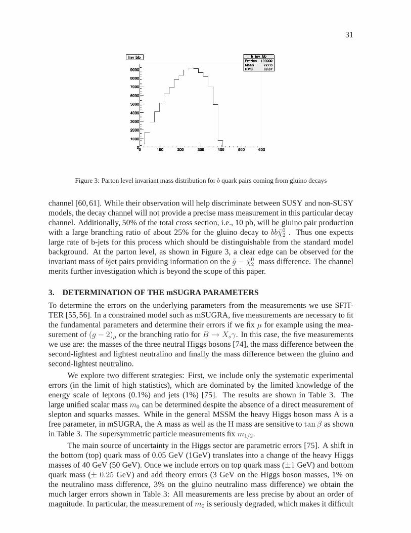
Figure 3: Parton level invariant mass distribution forb quark pairs coming from gluino decays

channel [60,61]. While their observation will help discriminate between SUSY and non-SUSYmodels, the decay channel will not provide a precise mass measurement in this particular decaychannel. Additionally, 50% of the total cross section, i.e., 10 pb, will be gluino pair productionwith a large branching ratio of about 25% for the gluino decayto bbχ0

2 . Thus one expectslarge rate of b-jets for this process which should be distinguishable from the standard modelbackground. At the parton level, as shown in Figure 3, a clearedge can be observed for theinvariant mass ofbjet pairs providing information on theg − χ0

2 mass difference. The channelmerits further investigation which is beyond the scope of this paper.

3. DETERMINATION OF THE mSUGRA PARAMETERS

To determine the errors on the underlying parameters from the measurements we use SFIT-TER [55,56]. In a constrained model such as mSUGRA, five measurements are necessary to fitthe fundamental parameters and determine their errors if wefix µ for example using the mea-surement of(g − 2)µ or the branching ratio forB → Xsγ. In this case, the five measurementswe use are: the masses of the three neutral Higgs bosons [74],the mass difference between thesecond-lightest and lightest neutralino and finally the mass difference between the gluino andsecond-lightest neutralino.

We explore two different strategies: First, we include onlythe systematic experimentalerrors (in the limit of high statistics), which are dominated by the limited knowledge of theenergy scale of leptons (0.1%) and jets (1%) [75]. The results are shown in Table 3. Thelarge unified scalar massm0 can be determined despite the absence of a direct measurement ofslepton and squarks masses. While in the general MSSM the heavy Higgs boson mass A is afree parameter, in mSUGRA, the A mass as well as the H mass are sensitive totan β as shownin Table 3. The supersymmetric particle measurements fixm1/2.

The main source of uncertainty in the Higgs sector are parametric errors [75]. A shift inthe bottom (top) quark mass of 0.05 GeV (1GeV) translates into a change of the heavy Higgsmasses of 40 GeV (50 GeV). Once we include errors on top quark mass (±1 GeV) and bottomquark mass (± 0.25 GeV) and add theory errors (3 GeV on the Higgs boson masses, 1%onthe neutralino mass difference, 3% on the gluino neutralinomass difference) we obtain themuch larger errors shown in Table 3: All measurements are less precise by about an order ofmagnitude. In particular, the measurement ofm0 is seriously degraded, which makes it difficult

32

nominal exp errors total errorm0 1400 50 610m1/2 180 2.2 14tan β 51 0.3 4.6A0 700 200 687

Table 3: The nominal values and the errors on the fundamentalparameters are shown for fits with experimental

errors only, and total Error.

or impossible to establish high-mass scalars. Most of this loss of precision is due to the lightestHiggs boson mass.

4. CONCLUSIONS

If supersymmetry should be realized with focus-point like properties, tri-leptons will be mea-sured at the LHC with good precision. Adding mass measurements of the three neutral Higgsscalars, we dan determine the SUSY breaking parameters withgood precision (assuming weknow how SUSY is broken). Once we adds the parametric as well as theoretical errors, theprecision decreases by an order of magnitude, and it will be difficult to establish heavy scalarswith our limited set of measurements.

Acknowledgements

Lauren Tompkins would like to thank the Franco-American Fulbright Commission for financingher work and stay in France. In addition she would like to thank LAL Orsay and the ATLASgroup for welcoming and supporting her as a member of the laboratory.

33

Part 6

Constraints on mSUGRA from indirectdark matter searches and the LHCdiscovery reachV. Zhukov

AbstractThe signal from annihilation of the relic neutralino in the galactic halocan be used as a constraint on the universal gaugino mass in mSUGRA.The excess of the diffusive gamma rays measured by the EGRET satel-lite limits the neutralino mass to the 40-100 GeV range. Together withother constraints, this will select a small region withm1/2 <250 GeVandm0 >1200 GeV at large tanβ=50-60. At the LHC this regioncan be studied via gluino and direct neutralino-chargino production forLint > 30fb−1.

1. INTRODUCTION

In the indirect Dark Matter (DM) search, the signal from DM annihilation can be observed as anexcess of gamma, positron or anti-protons fluxes on top of theCosmic Rays (CR) background,which is relatively small for these components. Existing experimental data on the diffusivegamma rays from the EGRET satellite and on positrons and anti-protons from the BESS, HEATand CAPRICE balloon experiments show a significant excess ofgamma with Eγ >2 GeV and,to a lesser extent, of positrons and anti-protons in comparison with the conventional Galacticmodel (CM) [76]. These excesses can be reduced, if one assumes that the locally measuredspectra are different from the average galactic ones [49]. This can be achieved by more than tensupernovae explosions in the vicinity of the solar system(∼ 100pc3) during last 10 Myr, whichis at the statistical limit. An alternative explanation is annihilation of relic DM in the GalacticDM halo. The flux of i-component (γ, e+, p) from annihilation can be written as:Fi(E) ∼ 1

m2χ

∫ρ2(r)B(r)Gi(E, ǫ, r)

∑

k < σkv > Aki (ǫ)drdǫ,

where< σkv > is the thermally averaged annihilation cross section into partonsk, Aki (ǫ)-hadronization of partonk into the final state ofi component,ρ(r) is the DM density distributionin the Galactic halo,B(r) is the local clumpiness of the DM, or ’boost’ factor,mχ is the massof the DM particle and theGi(E, e, r) is the propagation term (Gγ=1). The annihilation crosssection and the yield for each component can be calculated inthe frame of the mSUGRA modelwhere the DM particle is identified as a neutralino. The neutralino mass can be constrained bythe shape of the gamma energy spectrum. The DM profile times boost factorρ2(r)B(r) canbe reconstructed from the angular distributions of the gamma excess [77]. The independentmeasurement of the galactic rotation curve can be used to decouple the bulk profileρ(r) andthe clumpiness. The DM profile and the clumpiness are also connected to the cosmologicalscenario, in particular to the primary spectrum of density fluctuations [78]. The propagation ofthe annihilation products and the CR backgrounds can be calculated with a galactic model. Inthis study the DM annihilation was introduced into publiclyavailable code of the GALPROP

34

E, GeV1 10 210

rel.u

nits

-510

-410

-310

-210

-110

1

10

210

Yield [1/ann.]

- p

+ e

γ

[rel.unitsCR/FluxDMFlux- p

+ e

γ

=50β=150 tan1/2=1400 m0mSUGRA m

E, MeV1 10 210 310 410 510

MeV

-1

s-1

sr

-2 F

lux,

cm

2E

-210

-110

IC

brems.

0π

Gamma

EGRET

CM+DM

CM

DM

=55 GeVχ

=50 mβ=150 tan1/2=1400 m0mSUGRA m

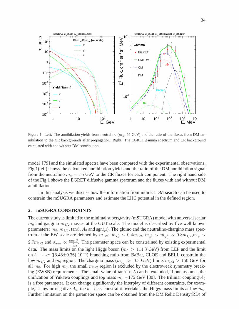
Figure 1: Left: The annihilation yields from neutralino (mχ=55 GeV) and the ratio of the fluxes from DM an-

nihilation to the CR backgrounds after propagation. Right:The EGRET gamma spectrum and CR background

calculated with and without DM contribution.

model [79] and the simulated spectra have been compared withthe experimental observations.Fig.1(left) shows the calculated annihilation yields and the ratio of the DM annihilation signalfrom the neutralinomχ = 55 GeV to the CR fluxes for each component. The right hand sideof the Fig.1 shows the EGRET diffusive gamma spectrum and thefluxes with and without DMannihilation.

In this analysis we discuss how the information from indirect DM search can be used toconstrain the mSUGRA parameters and estimate the LHC potential in the defined region.

2. mSUGRA CONSTRAINTS

The current study is limited to the minimal supergravity (mSUGRA) model with universal scalarm0 and gauginom1/2 masses at the GUT scale. The model is described by five well knownparameters:m0,m1/2, tanβ,A0 and sgn(µ). The gluino and the neutralino-chargino mass spec-trum at the EW scale are defined bym1/2: mχ0

1∼ 0.4m1/2, mχ0

2∼ mχ±

1∼ 0.8m1/2,m g ∼

2.7m1/2 andσann ∝ tan2βm4

1/2

. The parameter space can be constrained by existing experimental

data. The mass limits on the light Higgs boson (mh > 114.3 GeV) from LEP and the limiton b → sγ ([3.43±0.36] 10−4) branching ratio from BaBar, CLOE and BELL constrain thelow m1/2 andm0 region. The chargino mass (mχ±

1> 103 GeV) limitsm1/2 > 150 GeV for

all m0. For highm0, the smallm1/2 region is excluded by the electroweak symmetry break-ing (EWSB) requirements. The small value of tanβ < 5 can be excluded, if one assumes theunification of Yukawa couplings and top massmt ∼175 GeV [80]. The triliniar couplingA0

is a free parameter. It can change significantly the interplay of different constraints, for exam-ple, at low or negativeA0, theb → sγ constraint overtakes the Higgs mass limits at lowm0.Further limitation on the parameter space can be obtained from the DM Relic Density(RD) of

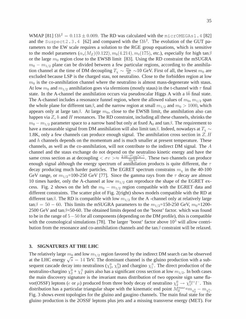
35

WMAP [81] Ωh2 = 0.113 ± 0.009. The RD was calculated with themicrOMEGAs1.4 [82]and theSuspect2.3.4 [62] and compared with theΩh2. The evolution of the GUT pa-rameters to the EW scale requires a solution to the RGE group equations, which is sensitiveto the model parameters (αs(MZ)(0.122), mb(4.214), mt(175), etc.), especially for high tanβor the largem0 region close to the EWSB limit [83]. Using the RD constraint the mSUGRAm0 − m1/2 plane can be divided between a few particular regions, according to the annihila-tion channel at the time of DM decouplingTχ ∼ mχ

20∼10 GeV. First of all, the lowestm0 are

excluded because LSP is the charged stau, not neutralino. Close to the forbidden region at lowm0 is the co-annihilation channel where the neutralino is almost mass-degenerate with staus.At low m0 andm1/2 annihilation goes via sfermions (mostly staus) in the t-channel withτ finalstate. In the A-channel the annihilation occurs via pseudoscalar Higgs A with abb final state.The A-channel includes a resonance funnel region, where theallowed values ofm0, m1/2 spanthe whole plane for different tanβ, and the narrow region at smallm1/2 andm0 > 1000, whichappears only at large tanβ. At largem0, close to the EWSB limit, the annihilation also canhappen viaZ, h andH resonances. The RD constraint, including all these channels, shrinks them0 −m1/2 parameter space to a narrow band but only at fixed A0 and tanβ. The requirement tohave a measurable signal from DM annihilation will also limit tanβ. Indeed, nowadays atTχ ∼1.8K, only a few channels can produce enough signal. The annihilation cross section inZ,Handh channels depends on the momentum and is much smaller at present temperature. Thesechannels, as well as the co-annihilation, will not contribute to the indirect DM signal. TheAchannel and the staus exchange do not depend on the neutralino kinetic energy and have thesame cross section as at decoupling< σv >≈ 2·10−27cm3s−1

Ωχh2 . These two channels can produceenough signal although the energy spectrum of annihilationproducts is quite different, theτdecay producing much harder particles. The EGRET spectrum constrainsmχ in the 40-100GeV range, orm1/2=100-250 GeV [77]. Since the gamma rays from theτ decay are almost10 times harder, only the A-channel at lowm1/2 can reproduce the shape of the EGRET ex-cess. Fig. 2 shows on the left them0 − m1/2 region compatible with the EGRET data anddifferent constraints. The scatter plot of Fig. 2(right) shows models compatible with the RD atdifferent tanβ. The RD is compatible with lowm1/2 for the A -channel only at relatively largetanβ = 50 − 60. This limits the mSUGRA parameters to them1/2=150-250 GeV,m0=1200-2500 GeV and tanβ=50-60. The obtained limits depend on the ’boost’ factor. which was foundto be in the range of5−50 for all components (depending on the DM profile), this is compatiblewith the cosmological simulations [78]. The larger ’boost’factor above 103 will allow contri-bution from the resonance and co-annihilation channels andthe tanβ constraint will be relaxed.

3. SIGNATURES AT THE LHC

The relatively largem0 and lowm1/2 region favored by the indirect DM search can be observedat the LHC energy

√s = 14 TeV. The dominant channel is the gluino production with a sub-

sequent cascade decay into neutralinos (χ02, χ

03) and charginoχ±

1 . The direct production of theneutralino-charginoχ0

2 + χ±1 pairs also has a significant cross section at lowm1/2. In both cases

the main discovery signature is the invariant mass distribution of two opposite sign same fla-vor(OSSF) leptons (e or µ) produced from three body decay of neutralinoχ0

2 → χ01l

+l−. Thisdistribution has a particular triangular shape with the kinematic end pointMmax

ll =mχ02−mχ0

1.

Fig. 3 shows event topologies for the gluino and gaugino channels. The main final state for thegluino production is the 2OSSF leptons plus jets and a missing transverse energy (MET). For

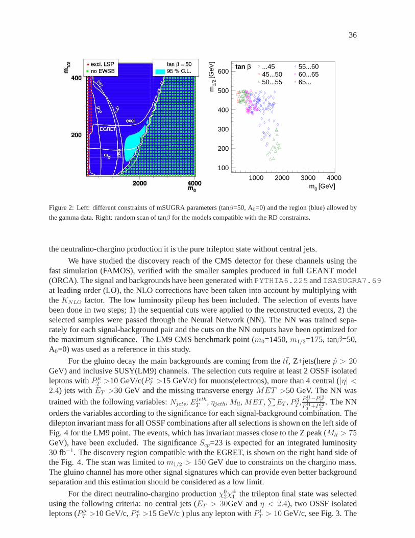
36

100

200

300

400

500

600

1000 2000 3000 4000m0 [GeV]

m1/

2 [G

eV]

tan β ...4545...5050...55

55...6060...6565...

Figure 2: Left: different constraints of mSUGRA parameters(tanβ=50, A0=0) and the region (blue) allowed by

the gamma data. Right: random scan of tanβ for the models compatible with the RD constraints.

the neutralino-chargino production it is the pure trilepton state without central jets.

We have studied the discovery reach of the CMS detector for these channels using thefast simulation (FAMOS), verified with the smaller samples produced in full GEANT model(ORCA). The signal and backgrounds have been generated withPYTHIA6.225 andISASUGRA7.69at leading order (LO), the NLO corrections have been taken into account by multiplying withtheKNLO factor. The low luminosity pileup has been included. The selection of events havebeen done in two steps; 1) the sequential cuts were applied tothe reconstructed events, 2) theselected samples were passed through the Neural Network (NN). The NN was trained sepa-rately for each signal-background pair and the cuts on the NNoutputs have been optimized forthe maximum significance. The LM9 CMS benchmark point (m0=1450,m1/2=175, tanβ=50,A0=0) was used as a reference in this study.

For the gluino decay the main backgrounds are coming from thett, Z+jets(herep > 20GeV) and inclusive SUSY(LM9) channels. The selection cuts require at least 2 OSSF isolatedleptons withP µ

T >10 GeV/c(P eT >15 GeV/c) for muons(electrons), more than 4 central (|η| <

2.4) jets withET >30 GeV and the missing transverse energyMET >50 GeV. The NN was

trained with the following variables:Njets, EjethT , ηjeth, Mll, MET ,

∑ET , P 3

T ,P l1

T −P l2T

P l1T +P l2

T

. The NN

orders the variables according to the significance for each signal-background combination. Thedilepton invariant mass for all OSSF combinations after allselections is shown on the left side ofFig. 4 for the LM9 point. The events, which has invariant masses close to the Z peak (Mll > 75GeV), have been excluded. The significanceScp=23 is expected for an integrated luminosity30 fb−1. The discovery region compatible with the EGRET, is shown onthe right hand side ofthe Fig. 4. The scan was limited tom1/2 > 150 GeV due to constraints on the chargino mass.The gluino channel has more other signal signatures which can provide even better backgroundseparation and this estimation should be considered as a lowlimit.

For the direct neutralino-chargino productionχ02χ

±1 the trilepton final state was selected

using the following criteria: no central jets (ET > 30GeV andη < 2.4), two OSSF isolatedleptons (P µ

T >10 GeV/c,P eT >15 GeV/c ) plus any lepton withP l

T > 10 GeV/c, see Fig. 3. The

37

Figure 3: Events topology at the LHC for the mSUGRA region compatible with the indirect DM search

(m1/2 <250 andm0 > 1000 GeV)

]2Dileptons invariant mass [GeV/c0 20 40 60 80 100 120 140

N/4

GeV

100

200

300

400

500

600

]2Dileptons invariant mass [GeV/c0 20 40 60 80 100 120 140

N/4

GeV

100

200

300

400

500

600

-1 L=30fb

±+e±µall

LM9 2l+X

bkg:SUSY

bkg: Wtjets

bkg: ttbar

bkg: Zjets

NN selection

2OSSF+X→~g+~g

=50)β=1450 tan0=175 m1/2

LM9 (m

-1 L=30fb

±+e±µall

LM9 2l+X

bkg:SUSY

bkg: Wtjets

bkg: ttbar

bkg: Zjets

]2[GeV/c0m0 1000 2000 3000

]2[G

eV/c

1/2

m

50

100

150

200

250

300

cpS

0 1000 2000 3000

50

100

150

200

250

300

0 1000 2000 3000

50

100

150

200

250

300

0 1000 2000 3000

50

100

150

200

250

300

0 1000 2000 3000

50

100

150

200

250

300

0 1000 2000 3000

50

100

150

200

250

300

0 1000 2000 3000

50

100

150

200

250

300

0 1000 2000 3000

50

100

150

200

250

300

=50β=0 tan0mSUGRA A

NO EWSB

2 < 114.3 GeV/cHiggsm

on-shell Z

2 < 103 GeV/c±1

χm 5

10

15

20

25

30

Figure 4: Left: Invariant mass of all OSSF lepton pairs for the mSUGRA gluino decays into at least oneχ02 for the

CMS LM9 point (m0=1450,m1/2=175, tanβ=50, A0=0). Right: Discovery reach inm0,m1/2 plane at tanβ=50

for Lint=30 fb−1, the significance Scp is shown as a color grades.

38

]2Dileptons invariant mass [GeV/c0 20 40 60 80 100 120 140

N/4

GeV

0

20

40

60

80

100

]2Dileptons invariant mass [GeV/c0 20 40 60 80 100 120 140

N/4

GeV

0

20

40

60

80

100 -1 L=30fb±+e±µall

LM9 3l

bkg: WWj

bkg:SUSY

bkg: Wtjets

bkg: ZZ

bkg: ZW

bkg: ttbar

bkg: Zjets

bkg: DY

NN selection

0

1χ ν 3l →±

1χ+0

2χ

=50)β=1450 tan0=175 m1/2

LM9 (m

-1 L=30fb±+e±µall

LM9 3l

bkg: WWj

bkg:SUSY

bkg: Wtjets

bkg: ZZ

bkg: ZW

bkg: ttbar

bkg: Zjets

bkg: DY

]2[GeV/c0m0 1000 2000 3000

]2[G

eV/c

1/2

m

50

100

150

200

250

300

cpS

0 1000 2000 3000

50

100

150

200

250

300

0 1000 2000 3000

50

100

150

200

250

300

0 1000 2000 3000

50

100

150

200

250

300

0 1000 2000 3000

50

100

150

200

250

300

0 1000 2000 3000

50

100

150

200

250

300

0 1000 2000 3000

50

100

150

200

250

300

0 1000 2000 3000

50

100

150

200

250

300

=50β=0 tan0mSUGRA A

NO EWSB

2 < 114.3 GeV/cHiggsm

on-shell Z

2 < 103 GeV/c±1

χm

3

4

5

6

7

8

Figure 5: Left: Invariant mass of all OSSF lepton pairs for the mSUGRA trilepton at the CMS LM9

point(m0=1450,m1/2=175, tanβ=50, A0=0). Right: Discovery reach inm0,m1/2 plane at tanβ=50 forLint=30

fb−1, the significance Scp is shown as a color grades.

MET cut, very effective for the background suppression in other SUSY channels, fails here asthe gauginos are light atm1/2 < 250 GeV. The main background comes from Z+jets, Drell Yan,

tt and ZW/ZZ production. The NN was trained with the variables:∑PT , P1,2,3

T , Θll, P 3T ,P l1

T −P l2T

P l1T +P l2

T

,

Mll, MET . The expected significance of the trilepton final state for the LM9 point isScp=6.1for Lint=30 fb−1 at low luminosity, see Fig. 5. At high luminosity the jets veto selection canreduce the signal selection efficiency by∼ 30% and another selection cuts are needed. Theright hand side of Fig. 5 shows the discovery reach of the trilepton final state.

Both channels, in spite of different event topology, have overlapping discovery regionsand are compatible with the region defined from indirect DM search.

4. CONCLUSIONS

The existing experimental data from the indirect DM search,together with the electroweak andrelic density constraints, limit the mSUGRA parameters to anarrow regionm1/2 ∼150-250GeV,m0 ∼1200-2500 GeV and tanβ ∼50-60. The LHC will probe this region at integratedluminosityLint >30 fb−1. The main discovery channels are the gluino decay intomχ0

2with

2OSSF dilepton plus jets final state and the neutralino-chargino direct production with the puretrilepton final state.

Acknowledgements

I would like to thanks my collaborators at Karlsruhe University W. de Boer, C. Sander, M.Niegel who share all results and T. Lari, A. Pukhov, M. Galanti, D. Kazakov for usefull discus-sions during and after the workshop.

39

Part 7

Relic density of dark matter in the MSSMwith CP violationG. Belanger, F. Boudjema, S. Kraml, A. Pukhov and A. Semenov

AbstractWe calculate the relic density of dark matter in the MSSM withCP vio-lation. Large phase effects are found which are due both to shifts in themass spectrum and to modifications of the couplings. We demonstratethis in scenarios where neutralino annihilation is dominated by heavyHiggs exchange.

1. INTRODUCTION

One of the interest of supersymmetric models with R-parity conservation is that they providea natural cold dark matter candidate, the lightest supersymmetric particle (LSP). The precisemeasurement of the relic density of dark matter by WMAP,0.0945 < Ωh2 < 0.1287 [2, 3]now strongly constrains the parameter space of supersymmetric models. Such is the case forexample in mSUGRA models, where the relic density of dark matter is often too large [4, 8,84–88]. It has been pointed out that if one allows the parameters of the MSSM to be complex,the relic density could be modified, even opening up new allowed regions of parameter space[89, 90]. Furthermore, the issue of CP violation in the MSSM is also interesting from thecosmological point of view as it provides a possible solution to the baryon number asymmetryvia the electroweak baryogenesis mechanism [91]. As a first step towards a comprehensivestudy of the relic density of dark matter in the MSSM with CP violation, we present here someresults for the case where the neutralino is the LSP and annihilates dominantly through heavyHiggs exchange.

2. THE MODEL

We consider the general MSSM with parameters defined at the weak scale. In general, one canhave complex parameters in the neutralino/chargino sectorwith Mi = |Mi|eiφi, µ = |µ|eiφµ

as well as for the trilinear couplings,Af = |Af |eiφf . The phase ofM2 can be rotated away.Among the trilinear couplings,At has the largest effect on the Higgs sector. Morever as thephase ofµ is the most severely constrained by electric dipole moment (EDM) measurements,we set it to zero and consider only the two remaining phases,φ1 andφt.

In the MSSM, the Higgs sector consists of two CP-even statesh0, H0 and one CP oddstateA. Adding CP violating phases in the model induces mixing between these three states.The mass eigenstatesh1, h2, h3 (mh1

< mh2< mh3

) are no longer eigenstates of CP. Themixing matrix is defined by

(φ1, φ2, a)Ta = Hai(h1, h2, h3)

Ti . (1)

In what follows we will mainly be concerned with the couplingof the lightest neutralino to Hig-gses that govern the neutralino annihilation cross sections via Higgs exchange. The Lagrangian

40

for such interactions writes

Lχ01χ0

1hi

=g

2

3∑

i=1

χ01(g

Shiχ0

1χ0

1+ iγ5g

Phiχ0

1χ0

1)χ0

1hi (2)

with the scalar part of the coupling

gShiχ01χ0

1= Re [(N∗

12 − tWN∗11) (H1iN

∗13 −H2iN

∗14 − iH3i(sβN

∗13 − cβN

∗14))] , (3)

whereN is the neutralino mixing matrix in the SLHA notation [92]. The pseudoscalar com-ponentgP

hiχ01χ0

1

corresponds to the imaginary part of the same expression. The LSP couplingsto Higgses will clearly be affected both by phases in the neutralino sector, for exampleφ1,which modifies the neutralino mixing, as well as from phases that enter the Higgs mixing.The latter can for example result from introducing a phase inthe trilinear couplingAt. In-deed in the MSSM the mixing is induced by loops involving top squarks and is proportional toIm(Atµ)/(m2

t2−m2

t1) [93]. Thus a large mixing is expected whenIm(Atµ) is comparable to

the squared of the stop masses. Note that the masses of the physical Higgses also depend onthe phase ofAt. In particular larger mass splitting between heavy Higgsesare found for largevalues ofµAt.

3. RELIC DENSITY OF DARK MATTER

The computation of the relic density of dark matter in supersymmetric models is now standard,and public codes are available which perform this calculation either in the context of the MSSMor of a unified model. Here we are using an extension ofmicrOMEGAs [5, 6] that allows forcomplex parameters in the MSSM [94]. UsingLanHEP [95], a new MSSM model file withcomplex parameters was rebuilt in theCalcHEP [96] notation, thus specifying all relevantFeynman rules. For the Higgs sector, an effective potentialis written in order to include in aconsistent way higher-order effects. Masses, mixing matrices and parameters of the effectivepotential are read directly fromCPsuperH [97] as well as masses and mixings of neutralinos,charginos and third generation sfermions. On the other handmasses of the first two genera-tions of sfermions are computed at tree-level from the inputparameters of the MSSM at theweak scale. All cross sections for annihilation and coannihilation processes are computed au-tomatically withCalcHEP , and the standardmicrOMEGAs routines are used to calculate theeffective annihilation cross section and the relic densityof dark matter.

The cross sections for some of the annihilation and coannihilation processes will dependon phases, and so will the thermally-averaged cross section. At the same time, the phaseschange the physical masses and so can strongly impact the value of the relic density, especiallywhen coannihilation processes are important or when annihilation occurs near a resonance. Itis the latter case that we will consider in more details here.

At vanishing relative velocity,v, neutralino annnihilation through s-channel exchange isp-wave suppressed; the annihilation proceeds strictly through pseudoscalar exchange. Never-theless when performing the thermal averaging, the scalar exchange cannot be neglected alto-gether. In the MSSM with real parameters it can amount toO(10%) of the total contribution.In the presence of phases both heavy Higgses can acquire a pseudoscalar component (that isgPhiχ0

1χ0

1

6= 0) and so bothh2 andh3 can significantly contribute to neutralino annihilation evenat smallv. There is a kind of sum rule that relates the couplings squared of the Higgses toneutralinos. Therefore, for the two heavy eigenstates which are in general close in mass, we do

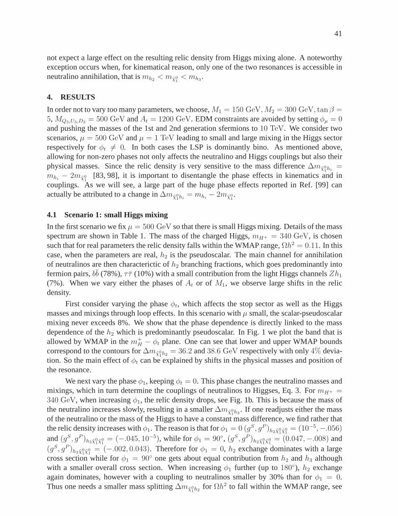
41

not expect a large effect on the resulting relic density fromHiggs mixing alone. A noteworthyexception occurs when, for kinematical reason, only one of the two resonances is accessible inneutralino annihilation, that ismh2

< mχ01< mh3

.

4. RESULTS

In order not to vary too many parameters, we choose,M1 = 150 GeV,M2 = 300 GeV, tanβ =5,MQ3,U3,D3

= 500 GeV andAt = 1200 GeV. EDM constraints are avoided by settingφµ = 0and pushing the masses of the 1st and 2nd generation sfermions to10 TeV. We consider twoscenarios,µ = 500 GeV andµ = 1 TeV leading to small and large mixing in the Higgs sectorrespectively forφt 6= 0. In both cases the LSP is dominantly bino. As mentioned above,allowing for non-zero phases not only affects the neutralino and Higgs couplings but also theirphysical masses. Since the relic density is very sensitive to the mass difference∆mχ0

1hi

=mhi

− 2mχ01

[83, 98], it is important to disentangle the phase effects inkinematics and incouplings. As we will see, a large part of the huge phase effects reported in Ref. [99] canactually be attributed to a change in∆mχ0

1hi

= mhi− 2mχ0

1.

4.1 Scenario 1: small Higgs mixing

In the first scenario we fixµ = 500 GeV so that there is small Higgs mixing. Details of the massspectrum are shown in Table 1. The mass of the charged Higgs,mH+ = 340 GeV, is chosensuch that for real parameters the relic density falls withinthe WMAP range,Ωh2 = 0.11. In thiscase, when the parameters are real,h2 is the pseudoscalar. The main channel for annihilationof neutralinos are then characterictic ofh2 branching fractions, which goes predominantly intofermion pairs,bb (78%),τ τ (10%) with a small contribution from the light Higgs channelsZh1

(7%). When we vary either the phases ofAt or of M1, we observe large shifts in the relicdensity.

First consider varying the phaseφt, which affects the stop sector as well as the Higgsmasses and mixings through loop effects. In this scenario with µ small, the scalar-pseudoscalarmixing never exceeds 8%. We show that the phase dependence isdirectly linked to the massdependence of theh2 which is predominantly pseudoscalar. In Fig. 1 we plot the band that isallowed by WMAP in them+

H − φt plane. One can see that lower and upper WMAP boundscorrespond to the contours for∆mχ0

1h2

= 36.2 and38.6 GeV respectively with only4% devia-tion. So the main effect ofφt can be explained by shifts in the physical masses and position ofthe resonance.

We next vary the phaseφ1, keepingφt = 0. This phase changes the neutralino masses andmixings, which in turn determine the couplings of neutralinos to Higgses, Eq. 3. FormH+ =340 GeV, when increasingφ1, the relic density drops, see Fig. 1b. This is because the mass ofthe neutralino increases slowly, resulting in a smaller∆mχ0

1h2

. If one readjusts either the massof the neutralino or the mass of the Higgs to have a constant mass difference, we find rather thatthe relic density increases withφ1. The reason is that forφ1 = 0 (gS, gP )h2χ0

1χ0

1= (10−5,−.056)

and(gS, gP )h3χ01χ0

1= (−.045, 10−5), while for φ1 = 90, (gS, gP )h2χ0

1χ0

1= (0.047,−.008) and

(gS, gP )h3χ01χ0

1= (−.002, 0.043). Therefore forφ1 = 0, h2 exchange dominates with a large

cross section while forφ1 = 90 one gets about equal contribution fromh2 andh3 althoughwith a smaller overall cross section. When increasingφ1 further (up to180), h2 exchangeagain dominates, however with a coupling to neutralinos smaller by 30% than forφ1 = 0.Thus one needs a smaller mass splitting∆mχ0

1h2

for Ωh2 to fall within the WMAP range, see

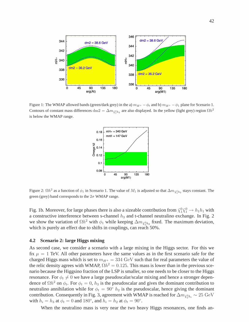
42

Figure 1: The WMAP allowed bands (green/dark grey) in the a)mH+ −φt and b)mH+ −φ1 plane for Scenario 1.

Contours of constant mass differencesdm2 = ∆mχ01h2

are also displayed. In the yellow (light grey) regionΩh2

is below the WMAP range.

Figure 2:Ωh2 as a function ofφ1 in Scenario 1. The value ofM1 is adjusted so that∆mχ01h2

stays constant. The

green (grey) band corresponds to the2σ WMAP range.

Fig. 1b. Moreover, for large phases there is also a sizeable contribution fromχ01χ

01 → h1h1 with

a constructive interference between s-channelh3 and t-channel neutralino exchange. In Fig. 2we show the variation ofΩh2 with φ1 while keeping∆mχ0

1h2

fixed. The maximum deviation,which is purely an effect due to shifts in couplings, can reach 50%.

4.2 Scenario 2: large Higgs mixing

As second case, we consider a scenario with a large mixing in the Higgs sector. For this wefix µ = 1 TeV. All other parameters have the same values as in the first scenario safe for thecharged Higgs mass which is set tomH+ = 334 GeV such that for real parameters the value ofthe relic density agrees with WMAP,Ωh2 = 0.125. This mass is lower than in the previous sce-nario because the Higgsino fraction of the LSP is smaller, soone needs to be closer to the Higgsresonance. Forφt 6= 0 we have a large pseudoscalar/scalar mixing and hence a stronger depen-dence ofΩh2 onφt. Forφt = 0, h3 is the pseudoscalar and gives the dominant contribution toneutralino annihilation while forφt = 90 h2 is the pseudoscalar, hence giving the dominantcontribution. Consequently in Fig. 3, agreement with WMAP is reached for∆mχ0

1hi∼ 25 GeV

with hi = h3 atφt = 0 and180, andhi = h2 atφt = 90.

When the neutralino mass is very near the two heavy Higgs resonances, one finds an-

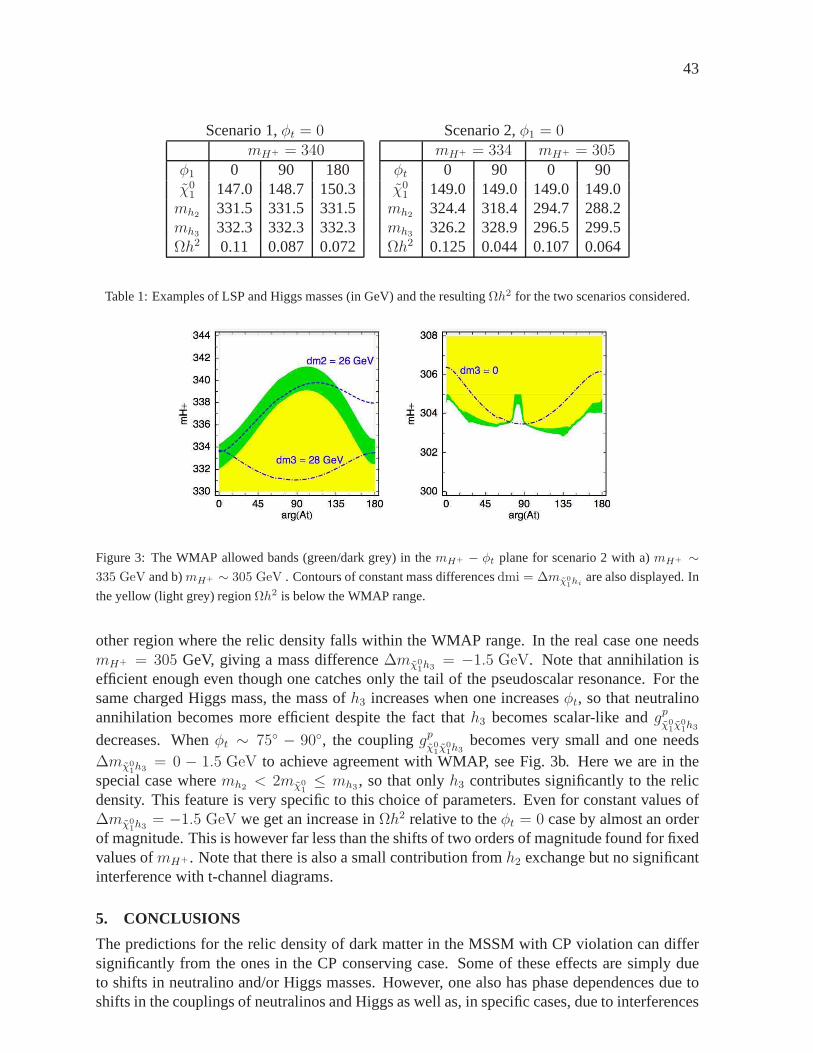
43

Scenario 1,φt = 0mH+ = 340

φ1 0 90 180χ0

1 147.0 148.7 150.3mh2

331.5 331.5 331.5mh3

332.3 332.3 332.3Ωh2 0.11 0.087 0.072

Scenario 2,φ1 = 0mH+ = 334 mH+ = 305

φt 0 90 0 90χ0

1 149.0 149.0 149.0 149.0mh2

324.4 318.4 294.7 288.2mh3

326.2 328.9 296.5 299.5Ωh2 0.125 0.044 0.107 0.064

Table 1: Examples of LSP and Higgs masses (in GeV) and the resulting Ωh2 for the two scenarios considered.

Figure 3: The WMAP allowed bands (green/dark grey) in themH+ − φt plane for scenario 2 with a)mH+ ∼335 GeV and b)mH+ ∼ 305 GeV . Contours of constant mass differencesdmi = ∆mχ0

1hiare also displayed. In

the yellow (light grey) regionΩh2 is below the WMAP range.

other region where the relic density falls within the WMAP range. In the real case one needsmH+ = 305 GeV, giving a mass difference∆mχ0

1h3

= −1.5 GeV. Note that annihilation isefficient enough even though one catches only the tail of the pseudoscalar resonance. For thesame charged Higgs mass, the mass ofh3 increases when one increasesφt, so that neutralinoannihilation becomes more efficient despite the fact thath3 becomes scalar-like andgp

χ01χ0

1h3

decreases. Whenφt ∼ 75 − 90, the couplinggpχ0

1χ0

1h3

becomes very small and one needs∆mχ0

1h3

= 0 − 1.5 GeV to achieve agreement with WMAP, see Fig. 3b. Here we are in thespecial case wheremh2

< 2mχ01≤ mh3

, so that onlyh3 contributes significantly to the relicdensity. This feature is very specific to this choice of parameters. Even for constant values of∆mχ0

1h3

= −1.5 GeV we get an increase inΩh2 relative to theφt = 0 case by almost an orderof magnitude. This is however far less than the shifts of two orders of magnitude found for fixedvalues ofmH+ . Note that there is also a small contribution fromh2 exchange but no significantinterference with t-channel diagrams.

5. CONCLUSIONS

The predictions for the relic density of dark matter in the MSSM with CP violation can differsignificantly from the ones in the CP conserving case. Some ofthese effects are simply dueto shifts in neutralino and/or Higgs masses. However, one also has phase dependences due toshifts in the couplings of neutralinos and Higgs as well as, in specific cases, due to interferences

44

between several contributions. Removing kinematical effects, we find a maximal deviation ofΩh2 of one order of magnitude. We have here only showed results for the case where theneutralinos annihilate via Higgs exchange. A systematic investigation of the different scenariosof neutralino annihilation (the cases of wino, Higgsino or mixed gaugino-Higgsino LSP, as wellas the case of coannihilation with stops or staus) includingCP violation is underway.

Acknowledgements

We thank J.S. Lee for his help with CPsuperH and W. Porod for discussions. This work wassupported in part by GDRI-ACPP of CNRS and by grants from the Russian Federal Agencyfor Science, NS-1685.2003.2 and RFBR-04-02-17448. A. P. acknowledges the hospitality ofCERN and LAPTH where some of the work contained here was performed. S.K. is supportedby an APART (Austrian Programme for Advanced Research and Technology) grant of the Aus-trian Academy of Sciences. She also acknowledges the financial support of CERN for theparticipation at the Les Houches Workshop.

45

Part 8

Light scalar top quarksC. Balazs∗, M. Carena, A. Finch, A. Freitas, S. Kraml, T. Lari, A. Menon,C. Milstene, S. Moretti,D.E. Morrissey, H. Nowak, G. Polesello, A.R. Raklev, C.H. Shepherd-Themistocleous, A. Sopczak∗

and C.E.M. Wagner∗ editors of this part.

1. INTRODUCTION

Most of the matter in the Universe consists of baryons and non-luminous (dark) matter. Theamount of these components are typically predicted independently from each other. In this sec-tion, we discuss the collider implications of a supersymmetric scenario that provides a commonorigin for both major components of matter. A cornerstone ofthis scenario is the assumptionthat the baryon asymmetry of the Universe is generated via electroweak baryogenesis. Thisassumption, in its minimal form, leads to a light scalar top quark, 100 GeV <∼ mt1

<∼ mt.If this light scalar top is found at colliders it can be a smoking gun signature of electroweakbaryogenesis.

After highlighting the basics and the consequences of the electroweak baryogenesis mech-anism in the Minimal Supersymmetric extension of the Standard Model (MSSM), in section 2.the viability that the MSSM simultaneously provides the measured baryon asymmetry and darkmatter abundance is summarized.

Then, in section 3. a new method is presented to discover a baryogenesis motivated lightscalar top, decaying dominantly intocχ0

1, at the LHC. The principal idea is to exploit the Ma-jorana nature of the gluino, which implies that gluinos do not distinguish betweentt∗1 and tt1combinations. This leads to like-sign top quarks in events of gluino pair production followedby gluino decays into top and stop.

This is followed by section 4. where a detailed analysis based on a parametrized simula-tion of the ATLAS detector is presented. A benchmark model isstudied in the framework ofthe MSSM, with a scalar top quark lighter than the top quark, yielding a final state similar tothe one fortt production. It is demonstrated that a signal for the stop canbe extracted in thiscase, and the kinematic features of the stop decay can be studied. A technique to subtract theStandard Model background based on the data is developed to achieve this result.

If scalar tops are light enough and are subject to large mixing effects, in the context of theMSSM, they may be produced at the LHC in pairs and in association with the lightest Higgsboson (decaying into bottom quark pairs). For the case in which top squarks are lighter than topquarks, they typically decay into charmed quarks and undetectable neutralinos. Thus the overallemerging signature is naturally composed of four isolated jets, two of which may be tagged asb-jets and two asc-jets, accompanied by sizable missing transverse energy. Two MSSM scenariosare considered in section 5., for which we investigate the behaviour of kinematic variables thatcould possibly be employed in the experimental selection ofsuch events.

Finally, scalar top quark studies at a Linear collider are presented in section 6.. Thecosmologically interesting scenario with small mass difference between the scalar top and theneutralino has been addressed in particular. The ILC will beable to explore this region effi-ciently. The simulation is based on a fast and realistic detector simulation. The scenario of

46

small mass differences is a challenge for c-quark tagging with a vertex detector. A vertex de-tector concept of the Linear Collider Flavor Identification(LCFI) collaboration, which studiesCCD detectors for quark flavor identification, is implemented in the simulations. The studyextends simulations for large mass differences (large visible energy).

2. BARYOGENSIS AND DARK MATTER

2.1 Overview of electroweak baryogenesis

The cosmological energy density of both main components of matter, baryons and dark matter,is known with a remarkable precision. Recent improvements of the astrophysical and cosmo-logical data, most notably due to the Wilkinson Microwave Anisotropy Probe (WMAP) [3],have determined the baryon density of the Universe (in unitsof the critical densityρc =3H2

0/(8πGN)) to beΩBh

2 = 0.0224 ± 0.0009, (1)

with h = 0.71+0.04−0.03. (HereH0 = h × 100 km/s/Mpc is the present value of the Hubble

constant, andGN is Newton’s constant.) According to the observations, the baryon density isdominated by baryons while anti-baryons are only secondaryproducts in high energy processes.The source of this baryon–anti-baryon asymmetry is one of the major puzzles of particle physicsand cosmology.

Assuming that inflation washes out any initial baryon asymmetry after the Big Bang, thereshould be a dynamic mechanism to generate the asymmetry after inflation. Any microscopicmechanism for baryogenesis must fulfill the three Sakharov requirements [100]:

• baryon number (B) violation,• CP violation, and• departure from equilibrium (unless CPT is violated [101]).

All three requirements are satisfied in both the SM and the MSSM during the electroweakphase transition. This is the basis for electroweak baryogenesis (EWBG) [102–106]. Whileelectroweak baryogenesis is viable in the MSSM, SM processes cannot generate a large enoughbaryon asymmetry during the electroweak phase transition.

Baryon number violation occurs in the SM and the MSSM due to quantum transitionsbetween inequivalent SU(2) vacua that violate(B+L) [107]. These transitions are exponentiallysuppressed at low temperatures in the electroweak broken phase [108, 109], but become activeat high temperatures when the electroweak symmetry is restored [110–114]. In the absence ofother charge asymmetries, like(B−L), they produce baryons and anti-baryons such that the netbaryon number relaxes to zero, and so do not by themselves generate a baryon asymmetry [115].

If the electroweak phase transition is first order, bubbles of broken phase nucleate withinthe symmetric phase as the Universe cools below the criticaltemperature. These provide thenecessary departure from equilibrium. EWBG then proceeds as follows [116]. CP violatinginteractions in the bubble walls generate chiral charge asymmetries which diffuse into the sym-metric phase in front of the walls. There, sphaleron transitions, which are active in the symmet-ric phase, convert these asymmetries into a net baryon number. This baryon number then dif-fuses into the bubbles where the electroweak symmetry is broken. The chiral charges producedin the bubble wall are able to diffuse into the symmetric phase, where they are approximatelyconserved, but not into the broken phase, where they are not.

Sphaleron transitions within the broken phase tend to destroy the baryon number gener-ated outside the bubble. To avoid this, the sphaleron transitions within the broken phase must

47

be strongly suppressed. This is the case provided the electroweak phase transition isstronglyfirst order [117],

v(Tc)/Tc >∼ 1, (2)

wherev(Tc) denotes the Higgs vacuum expectation value at the critical temperatureTc.

The strength of the electroweak phase transition may be determined by examining thefinite temperature effective Higgs boson potential. The Higgs vacuum expectation value at thecritical temperature is inversely proportional to the Higgs quartic coupling, related to the Higgsmass. For sufficiently light Higgs bosons, a first-order phase transition can be induced by theloop effects of light bosonic particles, with masses of the order of the weak scale and largecouplings to the Higgs fields. The only such particles in the SM are the gauge bosons, and theircouplings are not strong enough to induce a first-order phasetransition for a Higgs mass abovethe LEP-2 bound [118–120].

Within the MSSM, there are additional bosonic degrees of freedom which can make thephase transition more strongly first-order. The most important contribution comes from a lightstop, which interacts with the Higgs field with a coupling equal to the top-quark Yukawa. Inaddition, a light stop has six degrees of freedom, three of colour and two of charge, which furtherenhances the effect on the Higgs potential. Detailed calculations show that for the mechanismof electroweak baryogenesis to work, the lightest stop massmust be less than the top mass butgreater than about 120 GeV to avoid colour-breaking minima.Simultaneously, the Higgs bosoninvolved in breaking the electroweak symmetry must be lighter than 120 GeV [121–132], andonly slightly above the present experimental bound [133],

mh >∼ 114 GeV, (3)

which is valid for a SM Higgs boson.

The combined requirements of a first-order electroweak phase transition, strong enoughfor EWBG, and a Higgs boson mass above the experimental limitseverely restrict the allowedvalues of the stop parameters. To avoid generating too largea contribution to∆ρ, the light stopmust be mostly right-handed. Since the stops generate the most important radiative contributionto the Higgs boson mass in the MSSM [134–136], the other stop must be considerably heavierin order to raise the Higgs boson mass above the experimentalbound, Eq. (3). For the stop softsupersymmetry breaking masses, this implies [127]

m2U3<∼ 0, (4)

m2Q3>∼ (1 TeV)2.

whereU3 (Q3) is the soft mass of the third generation electroweak singlet up-type (doublet)scalar quarks at the electroweak scale. A similar balance isrequired for the combination of softSUSY breaking parameters defining the stop mixing,Xt = |At − µ∗/ tanβ|/mQ3

, andtanβ.Large values of these quantities tend to increase the Higgs mass at the expense of weakeningthe phase transition or the amount of baryon number produced. The allowed ranges have beenfound to be [127]

5 <∼ tanβ <∼ 10, (5)

0.3 <∼ |At − µ∗/ tanβ|/mQ3<∼ 0.5.

A strong electroweak phase transition is only a necessary condition for successful EWBG.In addition, a CP violating source is needed to generate a chiral charge asymmetry in the bubble

48

walls. Within the MSSM, the dominant source is produced by the charginos, and is proportionaltoℑ(µM2) [137–140]. For this source to be significant, the charginos must be abundant, whichrequires that they are not much heavier than the temperatureof the plasma,T ∼ Tc. Thistranslates into the following bounds:

| arg(µM2)| >∼ 0.1, (6)

µ,M2 <∼ 500 GeV.

These conditions are relevant to the abundance of neutralino dark matter, since the masses andmixing in the neutralino (and chargino) sector are stronglyaffected by the value of the softgaugino masses (Mi) and the higgsino mass parameter (µ) at the weak scale.

The need for a large CP violating phase, Eq. (6), implies thatparticular attention has to begiven to the violation of the experimental bounds on the electric dipole moments (EDM) of theelectron, neutron, and199Hg atom since phases enhance the EDM’s. The leading contributionsarise at the one loop level, and they all are mediated by an intermediate first or second generationsfermion. They become negligible if these sfermions are very heavy,mf

>∼ 10 TeV. Such largemasses have also only a very small effect on EWBG. At the two loop level, ifarg(µM2) 6= 0,there is a contribution involving an intermediate charginoand Higgs boson [141, 142]. SinceEWBG requires that this phase be non-zero and that the charginos be fairly light, the two loopcontribution is required for sufficient EWBG is to be successful. Thus, EDM limits stronglyconstrain the EWBG mechanism in the MSSM. Similarly, the branching ratio forb → sγdecays is also sensitive to this phase, and therefore imposes a further constraint on the EWBGmechanism.

2.2 Neutralino dark matter and electroweak baryogenesis

From the observations of the Wilkinson Microwave Anisotropy Probe (WMAP) [3], in agree-ment with the Sloan Digital Sky Survey (SDSS) [143], the darkmatter density of the Universecan be deduced as

ΩCDMh2 = 0.1126+0.0161

−0.0181, (7)

at95% CL. Since the SM cannot account for this, new physics has to beinvoked to explain darkmatter. This new physics has to accommodate non- standard, non-baryonic, massive, weaklyinteracting particles that make up the observable dark matter. Low energy supersymmetry pro-vides a consistent solution to the origin of dark matter and it has been extensively studied inthe literature in different scenarios of supersymmetry breaking [144–150]. In this summary,only the case when the lightest neutralinos make up all or part of the observed dark matter isconsidered in the MSSM.

In order to assess the viability of simultaneous generationof the observed baryon–anti-baryon asymmetry and dark matter, we focus on the narrow parameter region of the MSSMdefined by equations (3)-(6) of the previous section. As established earlier, in this parameterregion electroweak baryogenesis is expected to yield the observed amount of baryon density ofthe Universe. It is also assumed that the lightest neutralino is lighter than the light stop so that itis stable. To further simplify the analysis, we assume that the gaugino mass parametersM1 andM2 are related by the standard unification relation,M2 = (g2

2/g21)M1 ≃ 2M1. The first and

second generation sfermion soft masses are taken to be very large,mf>∼ 10 TeV, to comply

with the electron electric dipole moment (EDM) constraintsin the presence of sizable phases.Only a phase that is directly related to electroweak baryogenesis (EWBG) is introduced, namely

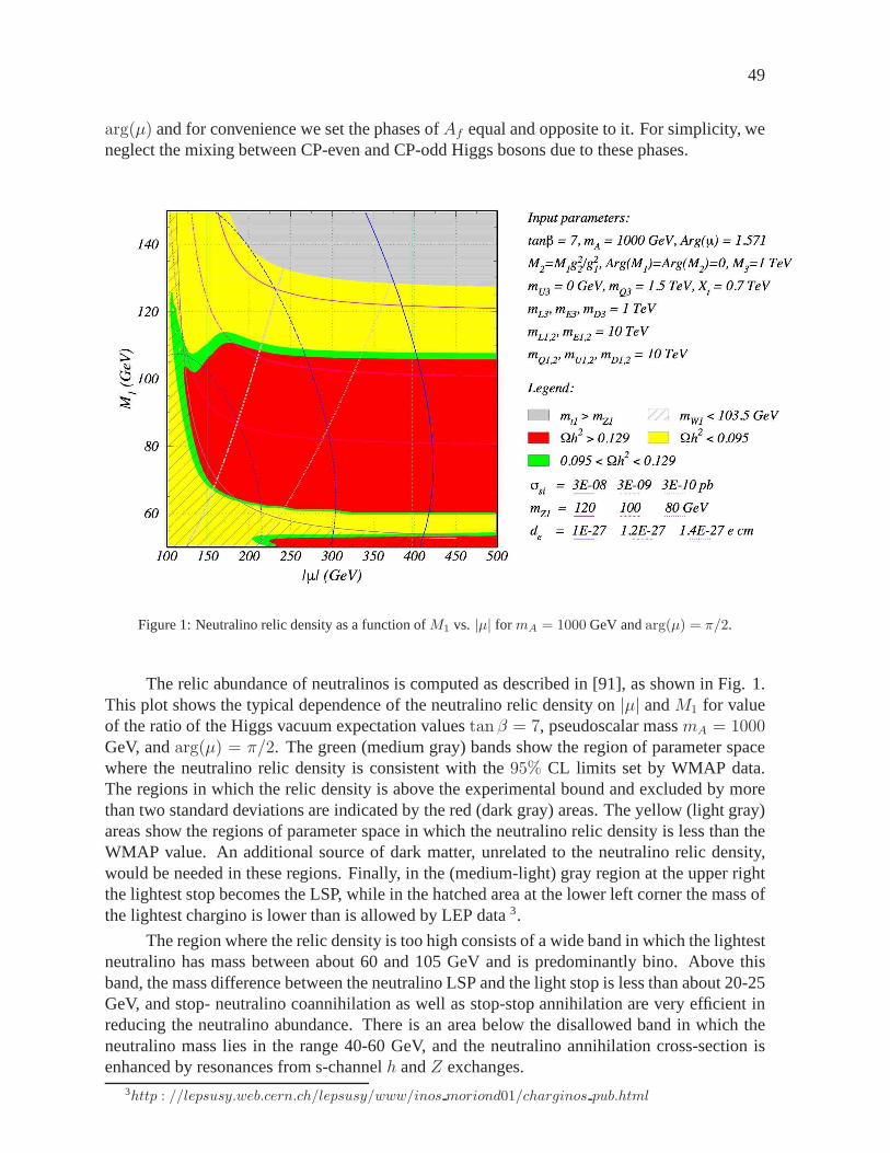
49

arg(µ) and for convenience we set the phases ofAf equal and opposite to it. For simplicity, weneglect the mixing between CP-even and CP-odd Higgs bosons due to these phases.

Figure 1: Neutralino relic density as a function ofM1 vs. |µ| for mA = 1000 GeV andarg(µ) = π/2.

The relic abundance of neutralinos is computed as describedin [91], as shown in Fig. 1.This plot shows the typical dependence of the neutralino relic density on|µ| andM1 for valueof the ratio of the Higgs vacuum expectation valuestan β = 7, pseudoscalar massmA = 1000GeV, andarg(µ) = π/2. The green (medium gray) bands show the region of parameter spacewhere the neutralino relic density is consistent with the95% CL limits set by WMAP data.The regions in which the relic density is above the experimental bound and excluded by morethan two standard deviations are indicated by the red (dark gray) areas. The yellow (light gray)areas show the regions of parameter space in which the neutralino relic density is less than theWMAP value. An additional source of dark matter, unrelated to the neutralino relic density,would be needed in these regions. Finally, in the (medium-light) gray region at the upper rightthe lightest stop becomes the LSP, while in the hatched area at the lower left corner the mass ofthe lightest chargino is lower than is allowed by LEP data3.

The region where the relic density is too high consists of a wide band in which the lightestneutralino has mass between about 60 and 105 GeV and is predominantly bino. Above thisband, the mass difference between the neutralino LSP and thelight stop is less than about 20-25GeV, and stop- neutralino coannihilation as well as stop-stop annihilation are very efficient inreducing the neutralino abundance. There is an area below the disallowed band in which theneutralino mass lies in the range 40-60 GeV, and the neutralino annihilation cross-section isenhanced by resonances from s-channelh andZ exchanges.

3http : //lepsusy.web.cern.ch/lepsusy/www/inos moriond01/charginos pub.html

50

The relic density is also quite low for smaller values of|µ|. In these regions, the neutralinoLSP acquires a significant Higgsino component allowing it tocouple more strongly to the Higgsbosons and theZ. This is particularly important in the region near(|µ|,M1) = (175, 110) GeVwhere the neutralino mass becomes large enough that annihilation into pairs of gauge bosonsthrough s-channel Higgs andZ exchange and t-channel neutralino and chargino exchange isallowed, and is the reason for the dip in the relic density near this point. Since the correspondingcouplings to the gauge bosons depend on the Higgsino contentof the neutralino, these decaychannels turn off as|µ| increases. For higherM1 values, the lightest neutralino and charginomasses are also close enough that chargino-neutralino coannihilation and chargino-charginoannihilation substantially increase the effective cross section.

As suggested by universalityM2 = (g22/g

21)M1 is used in Fig. 1. Thus, smaller values of

M1 andµ are excluded by the lower bound on the chargino mass from LEP data4, as indicatedby the hatched regions in the figures. This constraint becomes much less severe for larger valuesof the ratioM2/M1. We also find that increasing this ratio of gaugino masses (with M1 heldfixed) has only a very small effect on the neutralino relic density.

Figure 2: Spin independent neutralino-proton elastic scattering cross sections as a function of the neutralino mass

for arg(µ) = 0 (left) andarg(µ) = π/2 (right). The lower solid (cyan) lines indicate the projected sensitivity of

CDMS, ZEPLIN and XENON, respectively.

The search for weakly interacting massive particles is already in progress via detection oftheir scattering off nuclei by measuring the nuclear recoil. Since neutralinos are non-relativisticthey can be directly detected via the recoiling off a nucleusin elastic scattering. There are sev-eral existing and future experiments engaged in this search. The dependence of the neutralino-proton scattering cross section on the phase ofµ has been examined as shown in Fig. 2. A

4See the LEPSUSY web-page for combined LEP Chargino Results,up to 208 GeV.

51

random scan over the following range of MSSM parameters is conducted:5

−(80 GeV)2 < m2U3< 0, 100 < |µ| < 500 GeV, 50 < M1 < 150 GeV,

200 < mA < 1000 GeV, 5 < tan β < 10. (8)

The result of the scan, projected to the neutralino-proton scattering cross section versus neu-tralino mass plane, is shown by Fig. 2. The functionfσSI is plotted, wheref accounts for thediminishing flux of neutralinos with their decreasing density [151].

For models marked by yellow (light gray) dots the neutralinorelic density is below the2σWMAP bound, while models represented by green (medium gray)dots comply with WMAPwithin 2σ. Models that are above the WMAP value by more than2σ are indicated by red (darkgray) dots. The hatched area is excluded by the LEP chargino mass limit of 103.5 GeV. Thetop solid (blue) line represents the 2005 exclusion limit byCDMS [152]. The lower solid(cyan) lines indicate the projected sensitivity of the CDMS, ZEPLIN [153] and XENON [154]experiments.

Presently, the region above the (blue) top solid line is excluded by CDMS. In the nearfuture, forarg(µ) = 0, CDMS will probe part of the region of the parameter space where theWMAP dark matter bound is satisfied. The ZEPLIN experiment will start probing the stop-neutralino coannihilation region together with the annihilation region enhanced by s-channelAresonances. Finally, XENON will cover most of the relevant parameter space for small phases.Prospects for direct detection of dark matter tend to be weaker for large values of the phase ofµ, arg(µ) ≃ π/2.

Large phases, however, induce sizable corrections to the electron electric dipole moment.The EDM experiments are sensitive probes of this model [91].Presently the experimental upperlimit is

|de| < 1.6 × 10−27 e cm, (9)

at90% CL. One- and two loop contributions withO(1) phases, containing an intermediate firstgeneration slepton or charginos and Higgs bosons, respectively, are likely larger than this limit.The one loop diagrams are suppressed by choosing high first and second generation sfermionmasses in this work. The two loop corrections are suppressedby largemA or smalltanβ. Therange ofde values obtained in our scan are consistent with the the current electron EDM boundand EWBG. On the other hand, formA < 1000 GeV, about an order of magnitude improvementof the electron EDM bound,|de| < 0.2× 10−27 e cm, will be sufficient to test this baryogenesismechanism within the MSSM.

In summary, the requirement of a consistent generation of baryonic and dark matter inthe MSSM leads to a well-defined scenario, where, apart from alight stop and a light Higgsboson, neutralinos and charginos are light, sizeable CP violating phases, and moderate valuesof 5 <∼ tan β <∼ 10 are expected. These properties will be tested in a complementary way bythe Tevatron, the LHC and a prospective ILC, as well as through direct dark-matter detectionexperiments in the near future. The first tests of this scenario will probably come from electronEDM measurements, stop searches at the Tevatron and Higgs searches at the LHC within thenext few years.

5Parameters which are not scanned over are fixed as in the rightside of Fig. 1.

52

2.3 Baryogenesis inspired benchmark scenarios

The previous sections outlined a scenario in which the measured dark matter abundance andbaryon asymmetry of the Universe can simultaneously be achieved in the context of the MSSM.For the detailed exploration of the collider phenomenologyin this scenario, we follow the com-mon strategy of selecting and analysing individual parameter space points, or benchmark points.Some of the representative parameters of the selected points, which we call Les Houches scalartop (LHS) benchmark points, are presented in Table 1. The benchmark points are defined takeninto account the discussion of the the parameter values presented in the previous section.

All benchmark points are selected such that the baryon asymmetry of the Universe andthe relic density of neutralinos is predicted to be close to the one measured by WMAP and passall known low energy, collider and astronomy constraints. The most important of these are theSUSY particle masses, the electron EDM,B(b → sγ), and direct WIMP detection. A crucialconstraint is the LEP 2 Higgs boson mass limit ofmh > 114.4 GeV. In the calculations of thesupersymmetric spectrum and the baryon asymmetry, tree level relations are used except forthe Higgs mass, which is calculated at the one loop level. In the parameter region of interest,the one loop calculation results in about 6-8 GeV lower lightest Higgs mass than the two loopone [155, 156]. Thus, if the soft supersymmetric parametersdefining the benchmark points areused in a two loop calculation, the resulting lightest Higgsmass is found to be inconsistent withLEP 2. A two loop level consistency with the LEP 2 limit can be achieved only when a baryonasymmetry calculation becomes available using two loop Higgs boson masses.

The main difference between the benchmark points lies in themechanism that ensuresthat the neutralino relic density also complies with WMAP. Keeping the unification motivatedratio of the gaugino mass parametersM2/M1 close to 2 (together with the baryogenesis re-quired100 <∼ |µ| <∼ 500 GeV) induces a lightest neutralino with mostly bino admixture. A binotypically overcloses the Universe, unless there is a special situation that circumvents this. Forexample, as in the supergravity motivated minimal scenariomSUGRA, neutralinos can coan-nihilate with sfermions, resonant annihilate via Higgs bosons, or acquire a sizable Higgsinoadmixture in special regions of the parameter space. This lowers the neutralino density to alevel that is consistent with the observations.

Benchmark point LHS-1 features strong stop-neutralino coannihilation which lowers therelic density of neutralinos close to the WMAP central value. Sizable coannihilation only occurswhen the mass difference between the neutralino and stop is small (less than about 30-40%). Itis shown in the following sections that a small neutralino-stop mass gap poses a challenge forthe Tevatron and the LHC while the ILC can cover this region efficiently.

At benchmark LHS-2 resonant annihilation of neutralinos via s-channel Higgs resonanceslowers the neutralino abundance to the measured level. In this case, the neutralino mass must bevery close to half of the lightest Higss boson mass. This point features a stop that, given enoughluminosity, can be discovered at the Tevatron due to the large difference between the stop andthe neutralino masses. Even the heavier stop can possibly beproduced at the LHC together withthe third generation sleptons. On the other hand, since the resonance feature, the lightest Higgsboson can decay into neutralinos, which reduces its visiblewidth, and can make its discoverymore challenging.

Point LHS-3 satisfies the WMAP relic density constraint partly because the lightest neu-tralino acquires some wino admixture and because it is coannihilating with the lightest stop andchargino. The multiple effects lowering the relic density allow for a little larger neutralino-stop

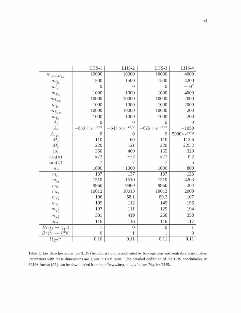
53

LHS-1 LHS-2 LHS-3 LHS-4mQ,U ,D1,2

10000 10000 10000 4000mQ3

1500 1500 1500 4200m2U3

0 0 0 −992

mD31000 1000 1000 4000

mL1,210000 10000 10000 2000

mL31000 1000 1000 2000

mE1,210000 10000 10000 200

mE31000 1000 1000 200

Ab 0 0 0 0At −650 × e−iπ/2 −643 × e−iπ/2 −676 × e−iπ/2 −1050

Ae,µ,τ 0 0 0 5000×eiπ/2M1 110 60 110 112.6M2 220 121 220 225.2|µ| 350 400 165 320

arg(µ) π/2 π/2 π/2 0.2tan(β) 7 7 7 5mA 1000 1000 1000 800mt1 137 137 137 123mt2 1510 1510 1510 4203me1 9960 9960 9960 204me2 10013 10013 10013 2000mχ0

1106 58.1 89.2 107

mχ02

199 112 145 196mχ+

1197 111 129 194

mχ+2

381 419 268 358mh 116 116 116 117

Br(t1 → χ01c) 1 0 0 1

Br(t1 → χ±1 b) 0 1 1 0

Ωχ01h2 0.10 0.11 0.11 0.11

Table 1: Les Houches scalar top (LHS) benchmark points motivated by baryogenesis and neutralino dark matter.

Parameters with mass dimensions are given in GeV units. The detailed definition of the LHS benchmarks, in

SLHA format [92], can be downloaded from http://www.hep.anl.gov/balazs/Physics/LHS/.

54

mass gap than in LHS-1. This point has a neutralino-stop massgap that makes it detectable atthe Tevatron and the LHC.

LHS-4, a variation of LHS-1, is defined in detail in Ref. [157]. Here the small neutralino-stop mass difference makes the light stop inaccessible at the Tevatron and the LHC. On theother hand, the ILC could measure the parameters with precision. The discovery potential ofthis point is discussed in detail in Section 6.

In summary, the four benchmark points offer various challenges for the three colliders.The Tevatron could resolve the stop quark in points LHS-2 andLHS-3, where thet1 decays intoχ±

1 b, but not in LHS-1 and LHS-4, where it decays intoχ01c with a small phase space. The LHC

on the other hand may explore LHS-1 via the method described in 3., and LHS-2 as describedin 4.. In principle these methods are also applicable for LHS-4 and LHS-3; the small massdifferences at these points, however, make the analysis much more difficult. In LHS-1, LHS-2and LHS-3 the LHC can pair produce the heavier stop, which is needed to pin down the stopsector so crucial for baryogenesis. At the ILC, one can perform precision measurements of thelight stop as shown in section 6. Moreover, the -ino sector including the important phase(s) canbe measured precisely (see [40] and references therein).

3. SAME-SIGN TOPS AS SIGNATURE OF LIGHT STOPS AT THE LHC

If the lighter of the two stops,t1, has a massmt1<∼ mt as motivated by baryogenesis [127,

158–160], gluino decays into stops and tops will have a largebranching ratio. Since gluinos areMajorana particles, they do not distinguish betweentt∗1 and tt1 combinations. Pair-producedgluinos therefore give

gg → tt t1t∗1, tt t

∗1t

∗1, tt t1t1 (10)

and hence same-sign top quarks in half of the gluino-to-stopdecays. Formt1 −mχ01< mW , the

t1 further decays intocχ01. If, in addition, theW stemming fromt → bW decays leptonically,

a signature of twob jets plus two same-sign leptons plus jets plus missing transverse energy isexpected:

pp→ gg → bb l+l+ (or bb l−l−) + jets + 6ET . (11)

This is a quite distinct peculiar signature, which will serve to remove most backgrounds, bothfrom SM and Supersymmetry. Even thought1 pair production has the dominant cross section,it leads to a signature of twoc-jets and missing transverse energy, which is of very limited use.Thus the same-sign top signature is of particular interest in our scenario. In this contribution,we lay out the basics of the analysis; for a detailed description see [161].

To investigate the use of our signature, Eq. (11), for discovering a lightt1 at the LHCwe define a MSSM benchmark point ‘LST-1’ withmg = 660 GeV, mt1 = 150 GeV andmχ0

1= 105 GeV. The other squarks (in particular the sbottoms) are taken to be heavier than

the gluinos. This considerably suppresses the SUSY background, and gluinos decay to about100% intott1. For the neutralino to have a relic density within the WMAP bound, we choosemA = 250 GeV. The MSSM parameters of LST-1 and the corresponding masses, calculatedwith SuSpect 2.3 [62], are given in Tables 2 and 3 (as for the LHS points, the SUSY-breakingparameters are taken to be onshell.). The relic density computed with micrOMEGAs [5, 6] isΩh2 = 0.105.

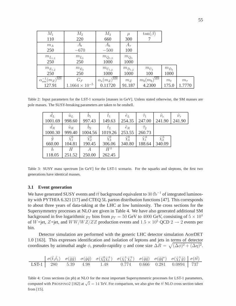
55

M1 M2 M3 µ tan(β)110 220 660 300 7mA At Ab Aτ250 −670 −500 100mL1,2

mL3mQ1,2

mQ3

250 250 1000 1000mE1,2

mE3mU1,2

mD1,2mU3

mD3

250 250 1000 1000 100 1000α−1

em(mZ)MS GF αs(mZ)MS mZ mb(mb)MS mt mτ

127.91 1.1664 × 10−5 0.11720 91.187 4.2300 175.0 1.7770

Table 2: Input parameters for the LST-1 scenario [masses in GeV]. Unless stated otherwise, the SM masses are

pole masses. The SUSY-breaking parameters are taken to be onshell.

dL uL b1 t1 eL τ1 νe ντ1001.69 998.60 997.43 149.63 254.35 247.00 241.90 241.90dR uR b2 t2 eR τ2

1000.30 999.40 1004.56 1019.26 253.55 260.73g χ0

1 χ02 χ0

3 χ04 χ±

1 χ±2

660.00 104.81 190.45 306.06 340.80 188.64 340.09h H A H±

118.05 251.52 250.00 262.45

Table 3: SUSY mass spectrum [in GeV] for the LST-1 scenario. For the squarks and sleptons, the first two

generations have identical masses.

3.1 Event generation

We have generated SUSY events andtt background equivalent to30 fb−1 of integrated luminos-ity with PYTHIA 6.321 [17] and CTEQ 5L parton distribution functions [47]. This correspondsto about three years of data-taking at the LHC at low luminosity. The cross sections for theSupersymmetry processes at NLO are given in Table 4. We have also generated additional SMbackground in five logarithmicpT bins frompT = 50 GeV to4000 GeV, consisting of5 × 104

of W+jet,Z+jet, andWW/WZ/ZZ production events and1.5 × 105 QCD 2 → 2 events perbin.

Detector simulation are performed with the generic LHC detector simulation AcerDET1.0 [163]. This expresses identification and isolation of leptons and jets in terms of detectorcoordinates by azimuthal angleφ, pseudo-rapidityη and cone size∆R =

√

(∆φ)2 + (∆η)2.

σ(t1t1) σ(gg) σ(gq) σ(χ02χ

±1 ) σ(χ±

1 χ∓1 ) σ(qq) σ(qq∗) σ(χ±

1 g) σ(tt)LST-1 280 5.39 4.98 1.48 0.774 0.666 0.281 0.0894 737

Table 4: Cross sections (in pb) at NLO for the most important Supersymmetric processes for LST-1 parameters,

computed with PROSPINO2 [162] at√s = 14 TeV. For comparison, we also give thett NLO cross section taken

from [15].

56

Cut 2lep 4jet plepT pjet

T 2b 6ET 2t SSSignalgg → tt t1t

∗1, tt t

∗1t

∗1, tt t1t1 10839 6317 4158 960 806 628 330

BackgroundSUSY 1406 778 236 40 33 16 5SM 25.3M 1.3M 35977 4809 1787 1653 12

Table 5: Number of events after cumulative cuts for30 fb−1 of integrated luminosity.

We identify a lepton ifpT > 5 (6) GeV and|η| < 2.5 for electrons (muons). A lepton is isolatedif it is a distance∆R > 0.4 from other leptons and jets, and the transverse energy deposited ina cone∆R = 0.2 around the lepton is less than10 GeV. Jets are reconstructed from clusters bya cone-based algorithm and are accepted if the jet haspT > 15 GeV in a cone∆R = 0.4. Thejets are recalibrated using a flavour-independent parametrization, optimized to give a scale forthe dijet decay of a light Higgs. Theb-tagging efficiency and light jet rejection are set accordingto thepT parametrization for a low luminosity environment, given in[164].

3.2 Signal isolation

The following cuts are applied:

• two same-sign leptons (e or µ) with plepT > 20 GeV.

• at least four jets withpjetT > 50 GeV, of which two areb-tagged.

• 6ET > 100 GeV.• The top quark content in the events is explored by demanding two combinations of the two

hardest leptons andb-jets that give invariant massesmbl < 160 GeV, which is consistentwith a top quark.

The effects of these cuts are shown in Table 5 where “2lep 4jet” is after detector simulation andcuts on two reconstructed and isolated leptons and four reconstructed jets; “2b” is the numberof events left after theb-jet cut, assuming ab-tagging efficiency of 43%; “6ET ” is the cut onmissing transverse energy and “SS” the requirement of two same-sign leptons. These cutsconstitute the signature of Eq. (11). The same-sign cut is ofcentral importance in removingthe SM background, which at this point consists only oftt events. The cuts on transversemomentum and top content “2t” are used to further reduce the background. We find that thegluino pair production, with leptonic top decay, is easily separated from both SM and SUSYbackgrounds.

We have assumed vanishing flavour-changing neutral currents (FCNCs), so that the anoma-lous couplings intgc andtgu vertices are effectively zero, i.e. there is no significant same-signtop production by FCNCs. To investigate other possible backgrounds we have used MadGraphII with the MadEvent event generator [165, 166]. The search has been limited to parton level,as we find no processes that can contribute after placing appropriate cuts. We have investigatedthe SM processes that can mimic a same-sign top pair by mis-tagging of jets or the productionof one or more additional leptons, as well as inclusive production of same-sign top pairs. Inparticular we have investigated the diffractive scattering qq → W±q′W±q′ and the productionof a top pair from gluon radiation in singleW productionqq′ → ttW±. We have also checkedthe production ofttl+l−, tttt, tttb, ttbt, tW−tW−, tW+tW+ andW±W±bbjj.Cuts on lep-tons and quarks have been placed as given above, and two lepton-quark pairs are required to be

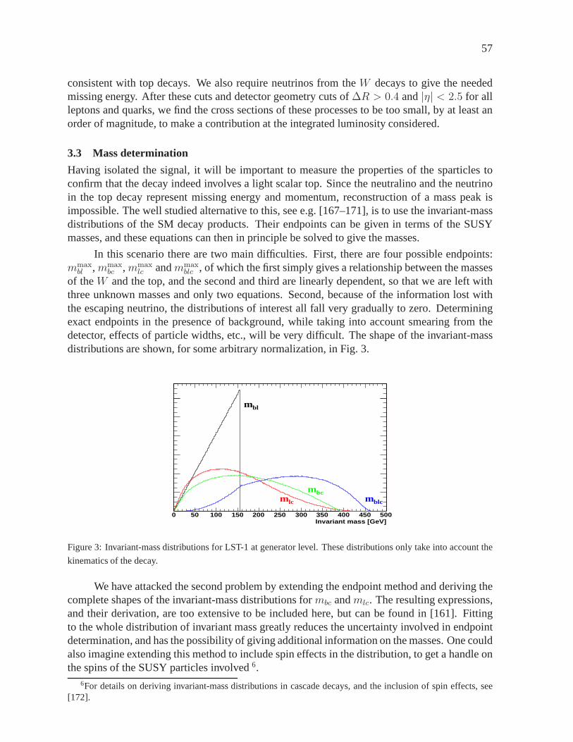
57

consistent with top decays. We also require neutrinos from theW decays to give the neededmissing energy. After these cuts and detector geometry cutsof ∆R > 0.4 and|η| < 2.5 for allleptons and quarks, we find the cross sections of these processes to be too small, by at least anorder of magnitude, to make a contribution at the integratedluminosity considered.

3.3 Mass determination

Having isolated the signal, it will be important to measure the properties of the sparticles toconfirm that the decay indeed involves a light scalar top. Since the neutralino and the neutrinoin the top decay represent missing energy and momentum, reconstruction of a mass peak isimpossible. The well studied alternative to this, see e.g. [167–171], is to use the invariant-massdistributions of the SM decay products. Their endpoints canbe given in terms of the SUSYmasses, and these equations can then in principle be solved to give the masses.

In this scenario there are two main difficulties. First, there are four possible endpoints:mmaxbl ,mmax

bc ,mmaxlc andmmax

blc , of which the first simply gives a relationship between the massesof theW and the top, and the second and third are linearly dependent,so that we are left withthree unknown masses and only two equations. Second, because of the information lost withthe escaping neutrino, the distributions of interest all fall very gradually to zero. Determiningexact endpoints in the presence of background, while takinginto account smearing from thedetector, effects of particle widths, etc., will be very difficult. The shape of the invariant-massdistributions are shown, for some arbitrary normalization, in Fig. 3.

Invariant mass [GeV]0 50 100 150 200 250 300 350 400 450 500

0

20

40

60

80

100

120

310×

blm

lcmbcm

blcm

Figure 3: Invariant-mass distributions for LST-1 at generator level. These distributions only take into account the

kinematics of the decay.

We have attacked the second problem by extending the endpoint method and deriving thecomplete shapes of the invariant-mass distributions formbc andmlc. The resulting expressions,and their derivation, are too extensive to be included here,but can be found in [161]. Fittingto the whole distribution of invariant mass greatly reducesthe uncertainty involved in endpointdetermination, and has the possibility of giving additional information on the masses. One couldalso imagine extending this method to include spin effects in the distribution, to get a handle onthe spins of the SUSY particles involved6.

6For details on deriving invariant-mass distributions in cascade decays, and the inclusion of spin effects, see[172].

58

In fitting thembc andmlc distributions, we start from the isolated gluino pair productionevents of Section 3.2. However, in some of these events one orboth of theW decay to a taulepton, which in turn decays leptonically; these are an additional, irreducible background tothe signal distributions. Theb-jets and leptons are paired through the cut on two top-quarkcandidates. A comparison with Monte Carlo information fromthe event generation shows thatthis works well in picking the right pairs. The issue remainsto identify thec-quark-initiatedjets and to assign these them to the correctb-jet and lepton pair. The precision of this endpointdetermination is limited by systematical uncertainties.

Different strategies can be used for picking thec-jets. Because of the strong correlationbetween the tagging ofb- andc-jets, one could use an inclusiveb/c-jet tagging where the twotypes of jets would be separated by theirb-tagging likelihoods, and the requirement of topcandidates in the event. A thorough investigation of this strategy will require a full simulationstudy, using realisticb-tagging routines. The strategy that we follow here is, instead, to accepta low b-tagging efficiency to pick twob-jets and reject mostc-jets. The likelihoods in theb-tagging routine could then help to pick the correctc-jets from the remaining jets. In this fastsimulation study we are restricted to a simple statistical model of the efficiency of makingthis identification and we assume a20% probability of identifying ac-jet directly from theb-tagging likelihood. For events where we have missed one or both of thec-jets, they areselected as the two hardest remaining jets withpjet

T < 100 GeV. This upper bound on transversemomentum is applied because the stop is expected to be relatively light if our signal exists, andit avoids picking jets from the decay of heavy squarks. Thec-jet candidates are paired to thetop candidates by their angular separation in the lab frame,and by requiring consistency withthe endpoints of the two invariant-mass distributions we are not looking at. For example, toconstruct thembc distribution, we demand consistency with the endpointsmmax

lc andmmaxblc

7.Events with no consistent combinations ofc-jets and top-quark candidates are rejected.

The fit functions formbc andmlc can in principle be used to determine both of the twolinearly independent parameters

(mmaxbc )2 =

(m2t −m2

W )(m2t1−m2

χ01

)(m21 +m2

2)

2m2tm

2t1

and a =m2

2

m21

, (12)

wherem2

1 = m2g −m2

t −m2t1

and m42 = m4

1 − 4m2tm

2t1. (13)

We typically havemtmt1 ≪ m2g for light stops, so thata ≈ 1. In our model the nominal value

is a = 0.991. The distributions are sensitive to such values ofa only at very low invariantmasses. Because of the low number of events, no sensible value can be determined from a fit;we therefore seta = 1. The fit quality and value ofmmax

bc is found to be insensitive to the choiceof a for a >∼ 0.980.

The results of the fits tommaxbc are shown in Fig. 4. The combined result of the two distri-

butions ismmaxbc = 389.8± 5.3 GeV, to be compared with the nominal value of391.1 GeV. The

somewhat largeχ2 values of the fits indicate that there are some significant systematical errors.However, if this is compared to the same fit with noc-tagging, we find large improvements inboth fit quality and distance from the nominal value. The analysis can be optimized using moredetailed information from theb-quark tagging.

7We require that the values are below the rough estimatesmmaxbc = 430 GeV, mmax

lc = 480 GeV andmmax

blc = 505 GeV, approximately 40 GeV above the nominal values, so no precise pre-determination of end-points is assumed.

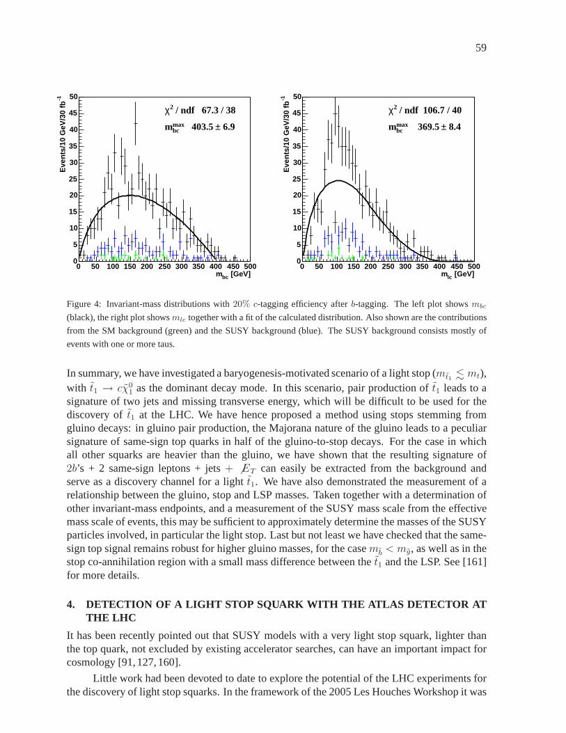
59

[GeV]bcm0 50 100 150 200 250 300 350 400 450 500

-1E

ven

ts/1

0 G

eV/3

0 fb

0

5

10

15

20

25

30

35

40

45

50

/ ndf 67.3 / 382χ

6.9± 403.5 maxbcm

[GeV]lcm0 50 100 150 200 250 300 350 400 450 500

-1E

ven

ts/1

0 G

eV/3

0 fb

0

5

10

15

20

25

30

35

40

45

50

/ ndf 106.7 / 402χ

8.4± 369.5 maxbcm

Figure 4: Invariant-mass distributions with20% c-tagging efficiency afterb-tagging. The left plot showsmbc

(black), the right plot showsmlc together with a fit of the calculated distribution. Also shown are the contributions

from the SM background (green) and the SUSY background (blue). The SUSY background consists mostly of

events with one or more taus.

In summary, we have investigated a baryogenesis-motivatedscenario of a light stop (mt1<∼ mt),

with t1 → cχ01 as the dominant decay mode. In this scenario, pair production of t1 leads to a

signature of two jets and missing transverse energy, which will be difficult to be used for thediscovery oft1 at the LHC. We have hence proposed a method using stops stemming fromgluino decays: in gluino pair production, the Majorana nature of the gluino leads to a peculiarsignature of same-sign top quarks in half of the gluino-to-stop decays. For the case in whichall other squarks are heavier than the gluino, we have shown that the resulting signature of2b’s + 2 same-sign leptons + jets+ 6ET can easily be extracted from the background andserve as a discovery channel for a lightt1. We have also demonstrated the measurement of arelationship between the gluino, stop and LSP masses. Takentogether with a determination ofother invariant-mass endpoints, and a measurement of the SUSY mass scale from the effectivemass scale of events, this may be sufficient to approximatelydetermine the masses of the SUSYparticles involved, in particular the light stop. Last but not least we have checked that the same-sign top signal remains robust for higher gluino masses, forthe casemb < mg, as well as in thestop co-annihilation region with a small mass difference between thet1 and the LSP. See [161]for more details.

4. DETECTION OF A LIGHT STOP SQUARK WITH THE ATLAS DETECTOR ATTHE LHC

It has been recently pointed out that SUSY models with a very light stop squark, lighter thanthe top quark, not excluded by existing accelerator searches, can have an important impact forcosmology [91,127,160].

Little work had been devoted to date to explore the potentialof the LHC experiments forthe discovery of light stop squarks. In the framework of the 2005 Les Houches Workshop it was

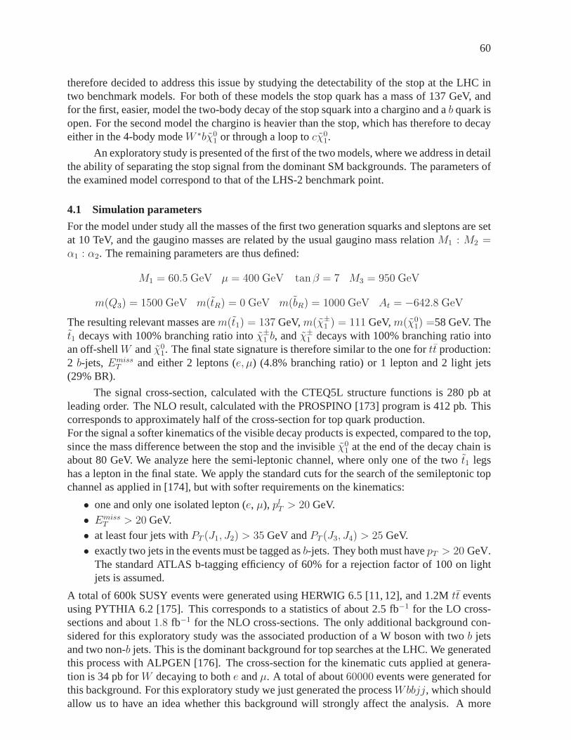
60

therefore decided to address this issue by studying the detectability of the stop at the LHC intwo benchmark models. For both of these models the stop quarkhas a mass of 137 GeV, andfor the first, easier, model the two-body decay of the stop squark into a chargino and ab quark isopen. For the second model the chargino is heavier than the stop, which has therefore to decayeither in the 4-body modeW ∗bχ0

1 or through a loop tocχ01.

An exploratory study is presented of the first of the two models, where we address in detailthe ability of separating the stop signal from the dominant SM backgrounds. The parameters ofthe examined model correspond to that of the LHS-2 benchmarkpoint.

4.1 Simulation parameters

For the model under study all the masses of the first two generation squarks and sleptons are setat 10 TeV, and the gaugino masses are related by the usual gaugino mass relationM1 : M2 =α1 : α2. The remaining parameters are thus defined:

M1 = 60.5 GeV µ = 400 GeV tanβ = 7 M3 = 950 GeV

m(Q3) = 1500 GeV m(tR) = 0 GeV m(bR) = 1000 GeV At = −642.8 GeV

The resulting relevant masses arem(t1) = 137 GeV,m(χ±1 ) = 111 GeV,m(χ0

1) =58 GeV. Thet1 decays with 100% branching ratio intoχ±

1 b, andχ±1 decays with 100% branching ratio into

an off-shellW andχ01. The final state signature is therefore similar to the one fortt production:

2 b-jets,EmissT and either 2 leptons (e, µ) (4.8% branching ratio) or 1 lepton and 2 light jets

(29% BR).

The signal cross-section, calculated with the CTEQ5L structure functions is 280 pb atleading order. The NLO result, calculated with the PROSPINO[173] program is 412 pb. Thiscorresponds to approximately half of the cross-section fortop quark production.For the signal a softer kinematics of the visible decay products is expected, compared to the top,since the mass difference between the stop and the invisibleχ0

1 at the end of the decay chain isabout 80 GeV. We analyze here the semi-leptonic channel, where only one of the twot1 legshas a lepton in the final state. We apply the standard cuts for the search of the semileptonic topchannel as applied in [174], but with softer requirements onthe kinematics:

• one and only one isolated lepton (e, µ), plT > 20 GeV.• Emiss

T > 20 GeV.• at least four jets withPT (J1, J2) > 35 GeV andPT (J3, J4) > 25 GeV.• exactly two jets in the events must be tagged asb-jets. They both must havepT > 20 GeV.

The standard ATLAS b-tagging efficiency of 60% for a rejection factor of 100 on lightjets is assumed.

A total of 600k SUSY events were generated using HERWIG 6.5 [11, 12], and 1.2Mtt eventsusing PYTHIA 6.2 [175]. This corresponds to a statistics of about 2.5 fb−1 for the LO cross-sections and about1.8 fb−1 for the NLO cross-sections. The only additional backgroundcon-sidered for this exploratory study was the associated production of a W boson with twob jetsand two non-b jets. This is the dominant background for top searches at theLHC. We generatedthis process with ALPGEN [176]. The cross-section for the kinematic cuts applied at genera-tion is 34 pb forW decaying to bothe andµ. A total of about60000 events were generated forthis background. For this exploratory study we just generated the processWbbjj, which shouldallow us to have an idea whether this background will strongly affect the analysis. A more

61

accurate estimate of this background should be performed bygenerating all of theWbb+(1,..n)jets with the appropriate matching to the parton shower. Thegenerated events are then passedthrough ATLFAST, a parametrized simulation of the ATLAS detector [18].

4.2 Analysis

After the described selection cuts the efficiency for thett background is 3.3%, forWbbjj 3.1%,and for the signal 0.47%, yielding a background which is about 15 times larger than the signal.An improvement of the signal/background ratio can be obtained by requiring on the minimuminvariant mass of all the non-b jetspT > 25 GeV in the event. The distribution for signal andbackground is shown in Fig. 5. A clear peak for the W mass is visible for the top background,

0

50

100

150

200

0 50 100 150 200 250m(jj)min

Eve

nts/

5 G

eV

0

1000

2000

3000

4000

0 50 100 150 200 250m(jj)min

Eve

nts/

5 G

eV

Figure 5: Minimum invariant mass distributions (in GeV) of two non-b jets for signal (left) and background (right).

whereas the invariant mass for the signal should be smaller than about 54 GeV, which is themass difference between theχ± and theχ0

1. In this analysis we are searching for the possibleevidence of a light stop, for which the decay through a resonantW is kinematically not allowed.It is therefore possible to significantly improve the signal/background ratio by selecting theevents wheremjj < 60 GeV. The signal/background ratio improves to 1/10, with a loss ofa bit more than half the signal. This cut could bias the kinematic distribution for the signal,which has a priori an unknown kinematics. We have therefore repeated the analysis for a cutat 70 GeV as a systematic check, obtaining equivalent results. Figure 6 shows them(bjj)min

distribution after this cut, i.e. the invariant mass for thecombination of a b-tagged jet andthe two non-b jets yielding the minimum invariant mass. If the selected jets result from thedecay of the stop, the invariant mass should have an end pointat about 79 GeV, whereas thecorresponding end-point should be at 175 GeV for the top background. The presence of the stopsignal is therefore visible as a shoulder in the distribution compared to the pure top contribution.A significant contribution fromWbb is present, without a particular structure. Likewise, thevariablem(bl)min has an end point at about 66 GeV for the signal and at 175 GeV forthe topbackground, as shown in Fig. 7. The same shoulder structure is observable. We need therefore

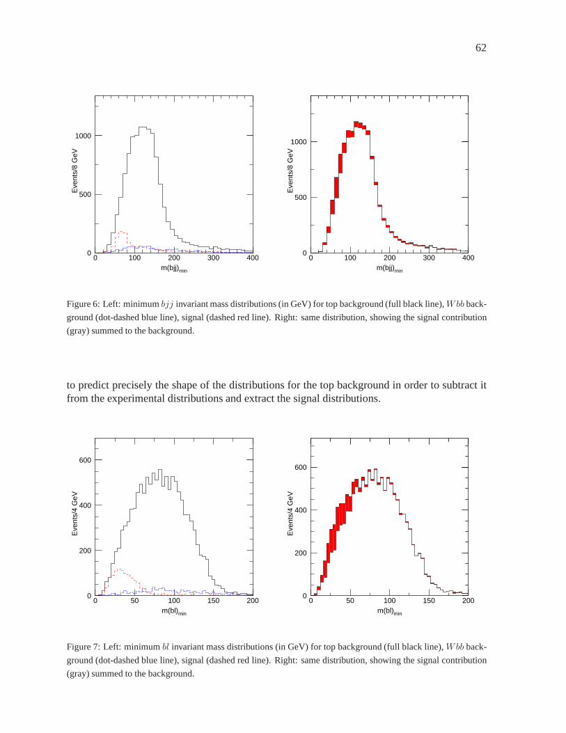
62

0

500

1000

0 100 200 300 400m(bjj)min

Eve

nts/

8 G

eV

0

500

1000

0 100 200 300 400m(bjj)min

Eve

nts/

8 G

eV

Figure 6: Left: minimumbjj invariant mass distributions (in GeV) for top background (full black line),Wbb back-

ground (dot-dashed blue line), signal (dashed red line). Right: same distribution, showing the signal contribution

(gray) summed to the background.

to predict precisely the shape of the distributions for the top background in order to subtract itfrom the experimental distributions and extract the signaldistributions.

0

200

400

600

0 50 100 150 200m(bl)min

Eve

nts/

4 G

eV

0

200

400

600

0 50 100 150 200m(bl)min

Eve

nts/

4 G

eV

Figure 7: Left: minimumbl invariant mass distributions (in GeV) for top background (full black line),Wbb back-

ground (dot-dashed blue line), signal (dashed red line). Right: same distribution, showing the signal contribution

(gray) summed to the background.

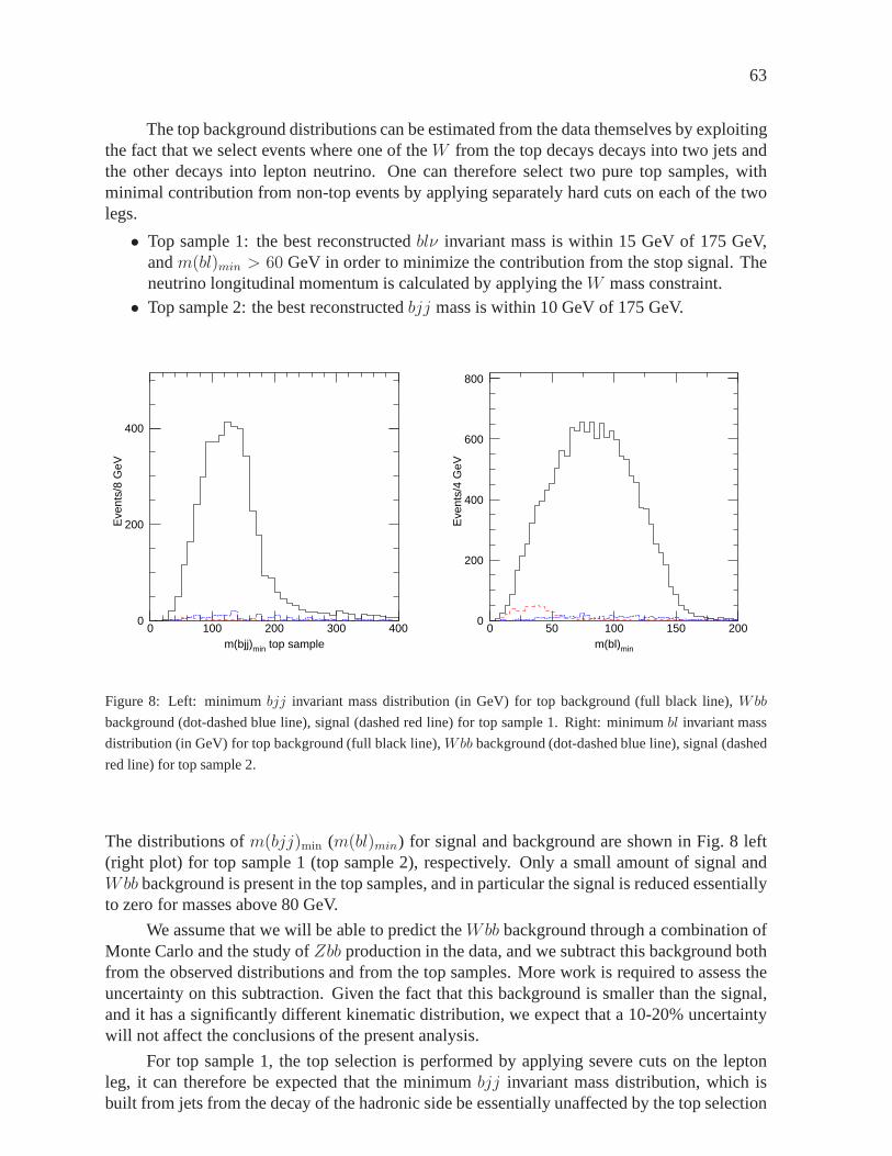
63

The top background distributions can be estimated from the data themselves by exploitingthe fact that we select events where one of theW from the top decays decays into two jets andthe other decays into lepton neutrino. One can therefore select two pure top samples, withminimal contribution from non-top events by applying separately hard cuts on each of the twolegs.

• Top sample 1: the best reconstructedblν invariant mass is within 15 GeV of 175 GeV,andm(bl)min > 60 GeV in order to minimize the contribution from the stop signal. Theneutrino longitudinal momentum is calculated by applying theW mass constraint.

• Top sample 2: the best reconstructedbjj mass is within 10 GeV of 175 GeV.

0

200

400

0 100 200 300 400m(bjj)min top sample

Eve

nts/

8 G

eV

0

200

400

600

800

0 50 100 150 200m(bl)min

Eve

nts/

4 G

eV

Figure 8: Left: minimumbjj invariant mass distribution (in GeV) for top background (full black line), Wbb

background (dot-dashed blue line), signal (dashed red line) for top sample 1. Right: minimumbl invariant mass

distribution (in GeV) for top background (full black line),Wbb background (dot-dashed blue line), signal (dashed

red line) for top sample 2.

The distributions ofm(bjj)min (m(bl)min) for signal and background are shown in Fig. 8 left(right plot) for top sample 1 (top sample 2), respectively. Only a small amount of signal andWbb background is present in the top samples, and in particular the signal is reduced essentiallyto zero for masses above 80 GeV.

We assume that we will be able to predict theWbb background through a combination ofMonte Carlo and the study ofZbb production in the data, and we subtract this background bothfrom the observed distributions and from the top samples. More work is required to assess theuncertainty on this subtraction. Given the fact that this background is smaller than the signal,and it has a significantly different kinematic distribution, we expect that a 10-20% uncertaintywill not affect the conclusions of the present analysis.

For top sample 1, the top selection is performed by applying severe cuts on the leptonleg, it can therefore be expected that the minimumbjj invariant mass distribution, which isbuilt from jets from the decay of the hadronic side be essentially unaffected by the top selection

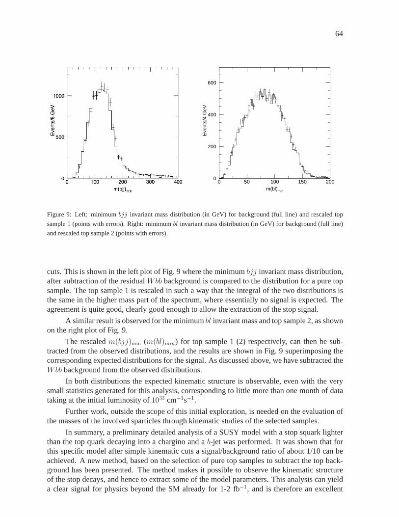
64

0

200

400

600

0 50 100 150 200m(bl)min

Eve

nts/

4 G

eV

Figure 9: Left: minimumbjj invariant mass distribution (in GeV) for background (full line) and rescaled top

sample 1 (points with errors). Right: minimumbl invariant mass distribution (in GeV) for background (full line)

and rescaled top sample 2 (points with errors).

cuts. This is shown in the left plot of Fig. 9 where the minimumbjj invariant mass distribution,after subtraction of the residualWbb background is compared to the distribution for a pure topsample. The top sample 1 is rescaled in such a way that the integral of the two distributions isthe same in the higher mass part of the spectrum, where essentially no signal is expected. Theagreement is quite good, clearly good enough to allow the extraction of the stop signal.

A similar result is observed for the minimumbl invariant mass and top sample 2, as shownon the right plot of Fig. 9.

The rescaledm(bjj)min (m(bl)min) for top sample 1 (2) respectively, can then be sub-tracted from the observed distributions, and the results are shown in Fig. 9 superimposing thecorresponding expected distributions for the signal. As discussed above, we have subtracted theWbb background from the observed distributions.

In both distributions the expected kinematic structure is observable, even with the verysmall statistics generated for this analysis, corresponding to little more than one month of datataking at the initial luminosity of1033 cm−1s−1.

Further work, outside the scope of this initial exploration, is needed on the evaluation ofthe masses of the involved sparticles through kinematic studies of the selected samples.

In summary, a preliminary detailed analysis of a SUSY model with a stop squark lighterthan the top quark decaying into a chargino and ab-jet was performed. It was shown that forthis specific model after simple kinematic cuts a signal/background ratio of about 1/10 can beachieved. A new method, based on the selection of pure top samples to subtract the top back-ground has been presented. The method makes it possible to observe the kinematic structureof the stop decays, and hence to extract some of the model parameters. This analysis can yielda clear signal for physics beyond the SM already for 1-2 fb−1, and is therefore an excellent

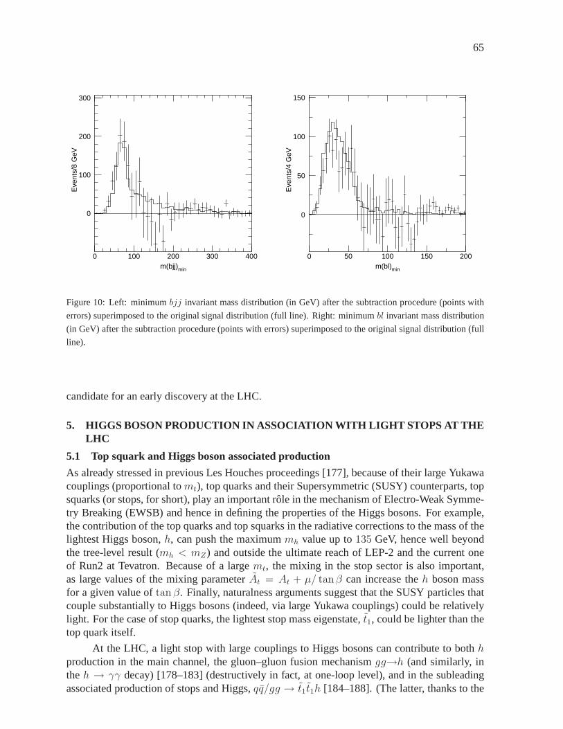
65

0

100

200

300

0 100 200 300 400m(bjj)min

Eve

nts/

8 G

eV

0

50

100

150

0 50 100 150 200m(bl)min

Eve

nts/

4 G

eV

Figure 10: Left: minimumbjj invariant mass distribution (in GeV) after the subtractionprocedure (points with

errors) superimposed to the original signal distribution (full line). Right: minimumbl invariant mass distribution

(in GeV) after the subtraction procedure (points with errors) superimposed to the original signal distribution (full

line).

candidate for an early discovery at the LHC.

5. HIGGS BOSON PRODUCTION IN ASSOCIATION WITH LIGHT STOPS AT THELHC

5.1 Top squark and Higgs boson associated production

As already stressed in previous Les Houches proceedings [177], because of their large Yukawacouplings (proportional tomt), top quarks and their Supersymmetric (SUSY) counterparts, topsquarks (or stops, for short), play an important role in themechanism of Electro-Weak Symme-try Breaking (EWSB) and hence in defining the properties of the Higgs bosons. For example,the contribution of the top quarks and top squarks in the radiative corrections to the mass of thelightest Higgs boson,h, can push the maximummh value up to135 GeV, hence well beyondthe tree-level result (mh < mZ) and outside the ultimate reach of LEP-2 and the current oneof Run2 at Tevatron. Because of a largemt, the mixing in the stop sector is also important,as large values of the mixing parameterAt = At + µ/ tanβ can increase theh boson massfor a given value oftan β. Finally, naturalness arguments suggest that the SUSY particles thatcouple substantially to Higgs bosons (indeed, via large Yukawa couplings) could be relativelylight. For the case of stop quarks, the lightest stop mass eigenstate,t1, could be lighter than thetop quark itself.

At the LHC, a light stop with large couplings to Higgs bosons can contribute to bothhproduction in the main channel, the gluon–gluon fusion mechanismgg→h (and similarly, intheh → γγ decay) [178–183] (destructively in fact, at one-loop level), and in the subleadingassociated production of stops and Higgs,qq/gg → t1t1h [184–188]. (The latter, thanks to the

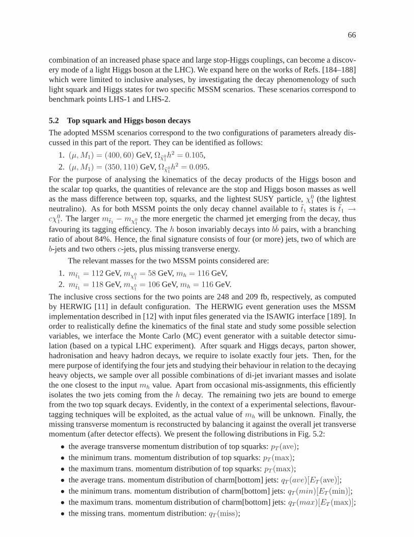
66

combination of an increased phase space and large stop-Higgs couplings, can become a discov-ery mode of a light Higgs boson at the LHC). We expand here on the works of Refs. [184–188]which were limited to inclusive analyses, by investigatingthe decay phenomenology of suchlight squark and Higgs states for two specific MSSM scenarios. These scenarios correspond tobenchmark points LHS-1 and LHS-2.

5.2 Top squark and Higgs boson decays

The adopted MSSM scenarios correspond to the two configurations of parameters already dis-cussed in this part of the report. They can be identified as follows:

1. (µ,M1) = (400, 60) GeV,Ωχ01h2 = 0.105,

2. (µ,M1) = (350, 110) GeV,Ωχ01h2 = 0.095.

For the purpose of analysing the kinematics of the decay products of the Higgs boson andthe scalar top quarks, the quantities of relevance are the stop and Higgs boson masses as wellas the mass difference between top, squarks, and the lightest SUSY particle,χ0

1 (the lightestneutralino). As for both MSSM points the only decay channel available tot1 states ist1 →cχ0

1. The largermt1 −mχ01

the more energetic the charmed jet emerging from the decay, thusfavouring its tagging efficiency. Theh boson invariably decays intobb pairs, with a branchingratio of about 84%. Hence, the final signature consists of four (or more) jets, two of which areb-jets and two othersc-jets, plus missing transverse energy.

The relevant masses for the two MSSM points considered are:

1. mt1 = 112 GeV,mχ01

= 58 GeV,mh = 116 GeV,2. mt1 = 118 GeV,mχ0

1= 106 GeV,mh = 116 GeV.

The inclusive cross sections for the two points are 248 and 209 fb, respectively, as computedby HERWIG [11] in default configuration. The HERWIG event generation uses the MSSMimplementation described in [12] with input files generatedvia the ISAWIG interface [189]. Inorder to realistically define the kinematics of the final state and study some possible selectionvariables, we interface the Monte Carlo (MC) event generator with a suitable detector simu-lation (based on a typical LHC experiment). After squark andHiggs decays, parton shower,hadronisation and heavy hadron decays, we require to isolate exactly four jets. Then, for themere purpose of identifying the four jets and studying theirbehaviour in relation to the decayingheavy objects, we sample over all possible combinations of di-jet invariant masses and isolatethe one closest to the inputmh value. Apart from occasional mis-assignments, this efficientlyisolates the two jets coming from theh decay. The remaining two jets are bound to emergefrom the two top squark decays. Evidently, in the context of aexperimental selections, flavour-tagging techniques will be exploited, as the actual value ofmh will be unknown. Finally, themissing transverse momentum is reconstructed by balancingit against the overall jet transversemomentum (after detector effects). We present the following distributions in Fig. 5.2:

• the average transverse momentum distribution of top squarks: pT (ave);• the minimum trans. momentum distribution of top squarks:pT (max);• the maximum trans. momentum distribution of top squarks:pT (max);• the average trans. momentum distribution of charm[bottom]jets: qT (ave)[ET (ave)];• the minimum trans. momentum distribution of charm[bottom]jets: qT (min)[ET (min)];• the maximum trans. momentum distribution of charm[bottom]jets:qT (max)[ET (max)];• the missing trans. momentum distribution:qT (miss);

67

• the trans. momentum distribution of the Higgs boson (from the two jets best reconstruct-ingmh): qT (Higgs);

• the invariant mass of the two jets best reconstructingmh: mbb.

The first three spectra have been obtained at parton level, while the others at detector level. Thedetector effects have been emulated by Gaussian smearing onthe lepton/photon and hadrontracks, according toσ(E)/E = res/

√

(E), with resolutionres = resEM = 0.1 andreshad = 0.5for the Electro-Magnetic (EM) and hadronic calorimeters, respectively. A cone jet algorithm isapplied to select the four jets by imposing∆Rj > 0.7 andpjT > 5 GeV. While the cut on az-imuth/pseudorapidity differences does emulate real detector performances the one on transversemomentum is clearly far too low. However, the main purpose ofthe simulation at this stage is toevaluate potential efficiencies of real LHC detectors by which the above cross sections shouldbe multiplied in order to have a realistic number of detectable events. Thus, as much as possibleof the phase space ought to be sampled, compatibly with the jet definition requirements. (Forthe same reason, individual jets are collected within the wide pseudorapidity range|ηj| < 5.)In this respect, it is obvious from the figure that the main source of lost signal events would bethe distributions in transverse momentum of thec-jets, particularly for point 2, for which theaforementioned mass difference is very small. Moreover, the missing transverse momentumdistributions peak at 50–60 GeV (somewhat softer for point 2, as expected), a value comfort-ably larger than typical background distributions yielding four (or more) jets in the detector butno leptons. Finally, apart from a low transverse energy taildue to misidentifiedb-jets (that maywell appear if flavour tagging techniques rejection efficiencies were poor), one should expectthe vast majority ofb-jets emerging fromh decays to pass standard detector thresholds. Thedistributions at parton level have been given for comparison with the results presented in theliterature referred to earlier.

In summary, on the basis of the above MC simulation, assumingthat b- andc-jets canbe collected starting frompjT = 30 GeV, and if one also requiresEmiss

T > 40 GeV, four-jet selection efficiencies should be around 50%(10%) for point 1(2). Above thepT cut LHCdetectors have large jet reconstruction efficiencies. Typical b tagging efficiencies are around50%, but charm tagging efficiencies will be lower than this. Given the inclusive cross sectionsand the above reconstruction efficiencies (not including tagging efficiencies), this leaves of order13,000(2,500) signal events with 100 fb−1 luminosity. This is a comfortable starting point inorder to refine a suitable selection for both MSSM configurations. We are planning to pursue afull detector analysis, also investigating higher jet multiplicities, in presence of additional cutson the jet system. Of course, at that stage, backgrounds willhave to be considered. However,a multi-jet plus missing transverse energy signal (with chiefly no energetic leptons) emergingfrom rather heavy particle decays (so jets are naturally separated) may offer several handlesto eventually extract a significant signal-to-background rate. In addition, trigger considerationswill be of primary importance to the signal selection. The mentioned analysis is now in progress.

6. SCALAR TOP QUARK AT A LINEAR COLLIDER

At a future International Linear Collider (ILC) the production and decay of scalar top quarks(stops) is particularly interesting for the development ofthe vertex detector as only two c-quarksand missing energy (from undetected neutralinos) are produced for light stops:

e+e− → t1¯t1 → c χ0

1 c χ01.

The scalar top Linear Collider studied have been recently reviewed [190].

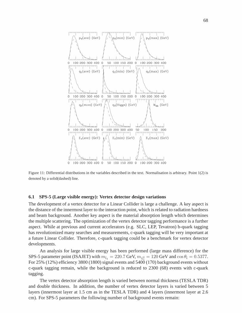
68

Figure 11: Differential distributions in the variables described in the text. Normalisation is arbitrary. Point 1(2) is

denoted by a solid(dashed) line.

6.1 SPS-5 (Large visible energy): Vertex detector design variations

The development of a vertex detector for a Linear Collider islarge a challenge. A key aspect isthe distance of the innermost layer to the interaction point, which is related to radiation hardnessand beam background. Another key aspect is the material absorption length which determinesthe multiple scattering. The optimization of the vertex detector tagging performance is a furtheraspect. While at previous and current accelerators (e.g. SLC, LEP, Tevatron) b-quark tagginghas revolutionized many searches and measurements, c-quark tagging will be very important ata future Linear Collider. Therefore, c-quark tagging couldbe a benchmark for vertex detectordevelopments.

An analysis for large visible energy has been performed (large mass difference) for theSPS-5 parameter point (ISAJET) withmt1 = 220.7 GeV,mχ0

1= 120 GeV andcos θt = 0.5377.

For 25% (12%) efficiency 3800 (1800) signal events and 5400 (170) background events withoutc-quark tagging remain, while the background is reduced to 2300 (68) events with c-quarktagging.

The vertex detector absorption length is varied between normal thickness (TESLA TDR)and double thickness. In addition, the number of vertex detector layers is varied between 5layers (innermost layer at 1.5 cm as in the TESLA TDR) and 4 layers (innermost layer at 2.6cm). For SPS-5 parameters the following number of background events remain:

69

Thickness layers 12% signal efficiency 25% signal efficiencyNormal 5 (4) 68 (82) 2300 (2681)Double 5 (4) 69 (92) 2332 (2765)

As a result, a significant larger number of background eventsis expected if the first layer ofthe vertex detector is removed. The distance of the first layer to the interaction point is also animportant aspect from the accelerator physics (beam delivery) perspective. The interplay be-tween the beam delivery and vertex detector design in regardto critical tolerances like hardwaredamage of the first layer and occupancy (unable to use the dataof the first layer) due to beambackground goes beyond the scope of this study and will be addressed in the future.

No significant increase in the expected background is observed for doubling the thicknessof the vertex detector layers. A first study with small visible energy shows a very similarresult [191] as described for larger visible energy.

6.2 SPS-5 (Large visible energy): Comparison of mass determinations

The precision in the scalar top mass determination at a Linear Collider is crucial and fourmethods are compared for the SPS-5 parameter point [192]. Two of the methods rely on accuratecross section measurements, the other two use kinematic information from the observed jets.

A high signal sensitivity is achieved with an Iterative Discriminant Analysis (IDA) me-thod [193]. The signal to background ratio is 10 or better. The expected size of the signal isbetween one thousand and two thousand events in 500fb−1 luminosity at a Linear Colliderwith

√s = 500 GeV [194]. These methods are used: a) beam polarization [195], b) threshold

scan, c) end point method, and d) minimum mass method [196]. The results of these methodsand basics characteristics are compared in Table 6.

Table 6: Comparison of precision for scalar top mass determination

Method ∆m (GeV) Luminosity CommentPolarization 0.57 2 × 500 fb−1 no theory errors includedThreshold scan 1.2 300 fb−1 right-handede− polarizationEnd point 1.7 500 fb−1

Minimum mass 1.5 500 fb−1 assumesmχ01

known

6.3 Small visible energy studies

In this section, the production of light stops at a 500 GeV Linear Collider is analyzed, usinghigh luminosityL = 500 fb−1 and polarization of both beams. The signature for stop pairproduction at ane+e− collider is two charm jets and large missing energy. For small ∆m, thejets are relatively soft and separation from backgrounds isvery challenging. Backgrounds aris-ing from various Standard Model processes can have cross-sections that are several orders ofmagnitude larger than the signal, so that even small jet energy smearing effects can be impor-tant. Thus, it is necessary to study this process with a realistic detector simulation. Signal andbackground events are generated with PYTHIA 6.129 [17], including a scalar top signal genera-tion [197] previously used in Ref. [194]. The detector simulation is based on the fast simulationSIMDET [198], describing a typical ILC detector.

In the first step a pre-selection is applied [157]. The signalis characterized by large miss-ing energy and transverse momentum from the two neutralinos, whereas for most backgrounds

70

Table 7: Background event numbers andt1¯t1 signal efficiencies (in %) for variousmt1 and∆m (in GeV) after

pre-selection and after several selection cuts [157]. In the last column the expected event numbers are scaled to a

luminosity of 500 fb−1.After Scaled to

Process Total presel. cut 1 cut 2 cut 3 cut 4 cut 5 cut 6 500 fb−1

W+W− 210,000 2814 827 28 25 14 14 8 145ZZ 30,000 2681 1987 170 154 108 108 35 257Weν 210,000 53314 38616 4548 3787 1763 1743 345 5044eeZ 210,000 51 24 20 11 6 3 2 36qq, q 6= t 350,000 341 51 32 19 13 10 8 160tt 180,000 2163 72 40 32 26 26 25 382-photon 3.2 × 106 1499 1155 1140 144 101 0 0 < 164mt1 = 140 :∆m = 20 50,000 68.5 48.8 42.1 33.4 27.9 27.3 20.9 9720∆m = 40 50,000 71.8 47.0 40.2 30.3 24.5 24.4 10.1 4700∆m = 80 50,000 51.8 34.0 23.6 20.1 16.4 16.4 10.4 4840mt1 = 180 :∆m = 20 25,000 68.0 51.4 49.4 42.4 36.5 34.9 28.4 6960∆m = 40 25,000 72.7 50.7 42.4 35.5 28.5 28.4 20.1 4925∆m = 80 25,000 63.3 43.0 33.4 29.6 23.9 23.9 15.0 3675mt1 = 220 :∆m = 20 10,000 66.2 53.5 53.5 48.5 42.8 39.9 34.6 2600∆m = 40 10,000 72.5 55.3 47.0 42.9 34.3 34.2 24.2 1815∆m = 80 10,000 73.1 51.6 42.7 37.9 30.3 30.3 18.8 1410

the missing momentum occurs from particles lost in the beam pipe. Therefore, cuts on the thrustangleθThrust, the longitudinal momentumplong,tot, the visible energyEvis and the total invariantmassminv are effective on all backgrounds.

Based on the above results from the experimental simulations, the discovery reach of a500 GeVe+e− collider can be estimated (Fig. 12). The signal efficienciesfor the parameterpoints in Fig. 12 are interpolated to cover the whole parameter region. Then, the signal ratesSare computed by multiplying the efficiencyǫ obtained from the simulations with the productioncross-section for each point(mt1 , mχ0

1). Together with the number of background eventsB,

this yields the significanceS/√S +B. The gray (green) area in the figure corresponds to the

5σ discovery region,S/√S +B > 5.

As evident from the figure, the ILC can find light stop quarks for mass differences downto ∆m ∼ O(5 GeV), beyond the stop-neutralino coannihilation region. The figure shows alsothe reach which can be achieved with small total luminosities.

6.4 Stop parameter determination

The discovery of light stops would hint toward the possibility of electroweak baryogenesis andmay allow the coannihilation mechanism to be effective. In order to confirm this idea, therelevant supersymmetry parameters need to be measured accurately. In this section, the exper-imental determination of the stop parameters will be discussed. The mass and its uncertaintyhas been determined with the polarization method:mt = 122.5 ± 1.0 GeV.

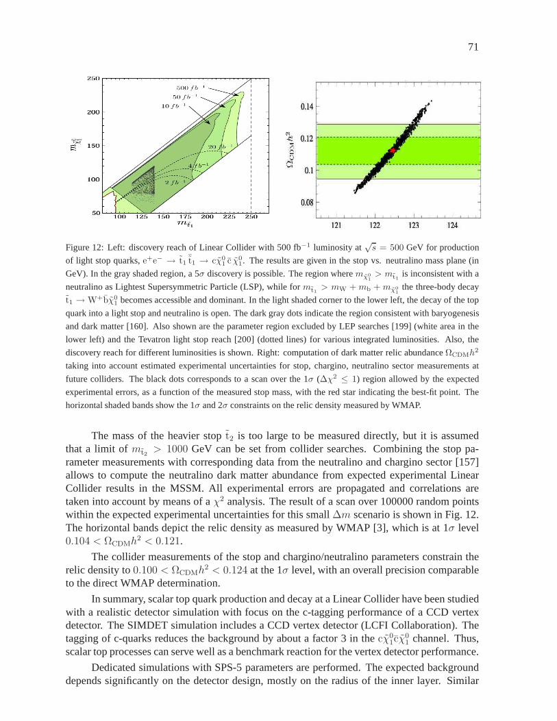
71

Figure 12: Left: discovery reach of Linear Collider with 500fb−1 luminosity at√s = 500 GeV for production

of light stop quarks,e+e− → t1¯t1 → cχ0

1 c χ01. The results are given in the stop vs. neutralino mass plane (in

GeV). In the gray shaded region, a 5σ discovery is possible. The region wheremχ01> mt1 is inconsistent with a

neutralino as Lightest Supersymmetric Particle (LSP), while for mt1 > mW +mb + mχ01

the three-body decay

t1 → W+bχ01 becomes accessible and dominant. In the light shaded cornerto the lower left, the decay of the top

quark into a light stop and neutralino is open. The dark gray dots indicate the region consistent with baryogenesis

and dark matter [160]. Also shown are the parameter region excluded by LEP searches [199] (white area in the

lower left) and the Tevatron light stop reach [200] (dotted lines) for various integrated luminosities. Also, the

discovery reach for different luminosities is shown. Right: computation of dark matter relic abundanceΩCDMh2

taking into account estimated experimental uncertaintiesfor stop, chargino, neutralino sector measurements at

future colliders. The black dots corresponds to a scan over the 1σ (∆χ2 ≤ 1) region allowed by the expected

experimental errors, as a function of the measured stop mass, with the red star indicating the best-fit point. The

horizontal shaded bands show the 1σ and 2σ constraints on the relic density measured by WMAP.

The mass of the heavier stopt2 is too large to be measured directly, but it is assumedthat a limit ofmt2 > 1000 GeV can be set from collider searches. Combining the stop pa-rameter measurements with corresponding data from the neutralino and chargino sector [157]allows to compute the neutralino dark matter abundance fromexpected experimental LinearCollider results in the MSSM. All experimental errors are propagated and correlations aretaken into account by means of aχ2 analysis. The result of a scan over 100000 random pointswithin the expected experimental uncertainties for this small ∆m scenario is shown in Fig. 12.The horizontal bands depict the relic density as measured byWMAP [3], which is at 1σ level0.104 < ΩCDMh

2 < 0.121.

The collider measurements of the stop and chargino/neutralino parameters constrain therelic density to0.100 < ΩCDMh

2 < 0.124 at the 1σ level, with an overall precision comparableto the direct WMAP determination.

In summary, scalar top quark production and decay at a LinearCollider have been studiedwith a realistic detector simulation with focus on the c-tagging performance of a CCD vertexdetector. The SIMDET simulation includes a CCD vertex detector (LCFI Collaboration). Thetagging of c-quarks reduces the background by about a factor3 in thecχ0

1cχ01 channel. Thus,

scalar top processes can serve well as a benchmark reaction for the vertex detector performance.

Dedicated simulations with SPS-5 parameters are performed. The expected backgrounddepends significantly on the detector design, mostly on the radius of the inner layer. Similar

72

results have been obtained from simulations of small mass differences between scalar top andneutralino.

For the scalar top mass determination four methods are compared and the polarizationmethod gives the highest precision. The other methods are also important as they contribute todetermine the properties of the scalar top quark. For example, the scalar character of the stopscan be established from the threshold cross section scan.

A new study for small mass difference, thus small visible energy, shows that a LinearCollider has a large potential to study the scalar top production and decay, in particular in thisexperimentally very challenging scenario.

From detailed simulations together with estimated errors for measurements in the neu-tralino and chargino sector [157], the expected cosmological dark matter relic density can becomputed. The precision at a Linear Collider will be similarto the current precision of WMAP.The uncertainty in the dark matter prediction from a Linear Collider is dominated by the mea-surement of scalar top quark mass.

7. CONCLUSIONS

New developments in scalar top studies have been discussed and four sets of Les HouchesScalar top (LHS) benchmarks sets have been defined. The strong cosmological motivation forlight scalar top quarks has been review and relevant aspectsfor the collider searches have beenemphasised. The search for scalar top quarks and measuring their properties will be an impor-tant task at future colliders. The experimental simulations show that like-sign top signaturescould be detected as signals for scalar top production at theLHC. In a second LHC study it hasbeen shown that light scalar tops could be observed already with low luminosity, possibly aftera few months of data- taking. For the future Linear Collider aspects of the detector design havebeen addressed with c-quark tagging as a benchmark for the vertex detector optimization. Dif-ferent methods of scalar top masses reconstruction have been compared and for cosmologicalinteresting parameter region, the ILC could achieve a similar precision on the relic dark matterdensity as the current WMAP measurements. Both at the LHC andthe ILC, scalar top studiescontinue to be an active and progressing field of research.

Acknowledgements

Research at the HEP Division of ANL is supported in part by theUS DOE, Division of HEP,Contract W-31-109-ENG-38. Fermilab is operated by Universities Research Association Inc.under contract no. DE-AC02-76CH02000 with the DOE.

S.K. is supported by an APART (Austrian Programme of Advanced Research and Tech-nology) grant of the Austrian Academy of Sciences. She also acknowledges the financial sup-port of CERN for the participation at the Les Houches 2005 Workshop. A.R. is supported bythe Norwegian Research Council.

T.L and G.P. thank members of the ATLAS Collaboration for helpful discussions. T.Land G.P. have made use of ATLAS physics analysis and simulation tools which are the result ofcollaboration-wide efforts.

A.S. acknowledges the support from PPARC and Lancaster University grants.

The authors are grateful to the Les Houches workshop organisers for their invitation andsupport throughout. We also thank S. Heinemeyer and G. Weiglein for useful suggestions.

73

Part 9

Identifying nonminimal neutralinos incombined LHC and ILC analysesS. Hesselbach, F. Franke, H. Fraas and G. Moortgat-Pick

AbstractThe measurement of the masses and production cross sectionsof thelight charginos and neutralinos at thee+e− International Linear Col-lider (ILC) with

√s = 500 GeV may not be sufficient to identify the

mixing character of the particles and to distinguish between the minimaland nonminimal supersymmetric standard model. We discuss asuper-symmetric scenario where the interplay with experimental data fromthe LHC might be essential to identify the underlying supersymmetricmodel.

1. INTROCUCTION

The Next-to-minimal Supersymmetric Standard Model NMSSM is the simplest extension ofthe MSSM by an additional Higgs singlet field. It contains fiveneutralinosχ0

i , the mass eigen-states of the photino, zino and neutral higgsinos, and two charginosχ±

i , being mixtures of winoand charged higgsino. The neutralino/chargino sector depends at tree level on six parameters:the U(1) and SU(2) gaugino massesM1 andM2, the ratiotan β of the vacuum expectationvalues of the doublet Higgs fields, the vacuum expectation value x of the singlet field and thetrilinear couplingsλ andκ in the superpotential, where the productλx = µeff replaces theµ-parameter of the MSSM [201–204]. The additional fifth neutralino may significantly changethe phenomenology of the neutralino sector. In scenarios where the lightest supersymmetricparticle is a nearly pure singlino, the existence of displaced vertices may lead to a particularlyinteresting experimental signature [205–208] which allows the distinction between the models.If however, only a part of the particle spectrum is kinematically accessible this distinction maybecome challenging. In this contribution we analyze an NMSSM scenario where the Higgs sec-tor and mass and cross section measurements in the neutralino sector do not allow to distinguishthe models, but only a combined analysis of LHC and ILC data.

2. STARTING POINT: NMSSM SCENARIO

We start with an NMSSM scenario with the parameters

M1 = 360 GeV, M2 = 147 GeV, tan β = 10, λ = 0.5, x = 915 GeV, κ = 0.2. (1)

74

and the following gaugino/higgsino masses and eigenstates:

mχ01

= 138 GeV, χ01 = (−0.02,+0.97,−0.20,+0.09,−0.07), (2)

mχ02

= 337 GeV, χ02 = (+0.62,+0.14,+0.25,−0.31,+0.65), (3)

mχ03

= 367 GeV, χ03 = (−0.75,+0.04,+0.01,−0.12,+0.65), (4)

mχ04

= 468 GeV, χ04 = (−0.03,+0.08,+0.70,+0.70,+0.08), (5)

mχ05

= 499 GeV, χ05 = (+0.21,−0.16,−0.64,+0.62,+0.37), (6)

where the neutralino eigenstates are given in the basis(B0, W 0, H01 , H

02 , S). As can be seen

from Eqs. (3) and (4), the particlesχ02 and χ0

3 have a rather strong singlino admixture. Thisscenario translates at thee+e− International Linear Collider (ILC) with

√s = 500 GeV into the

experimental observables of Table 1 for the measurement of the masses and production crosssections for several polarization configurations of the light neutralinos and charginos. We as-sume mass uncertainties ofO(1−2%), a polarization uncertainty of∆Pe±/Pe± = 0.5% and onestandard deviation statistical errors. The masses and cross sections in different beam polariza-tion configurations provide the experimental input for deriving the supersymmetric parameterswithin the MSSM using standard methods [26,27]. Note that beam polarization may be crucialfor distinguishing the two models [209–211].

Table 1: Masses with 1.5% (χ02,3, eL,R, νe) and 2% (χ0

1, χ±

1 ) uncertainty and cross sections with an error com-

posed of the error due to the mass uncertainties, polarization uncertainty of∆Pe±/Pe± = 0.5% and one stan-

dard deviation statistical error based on∫L = 100 fb−1, for both unpolarized beams and polarized beams with

(Pe− , Pe+) = (∓90%,±60%), in analogy to the study in [75].

mχ01=138±2.8 GeV σ(e+e− → χ±

1 χ∓1 )/fb σ(e+e− → χ0

1χ02)/fb

mχ02=337±5.1 GeV (Pe− , Pe+)

√s = 400 GeV

√s = 500 GeV

√s = 500 GeV

mχ±1

=139±2.8 GeV Unpolarized 323.9 ± 33.5 287.5 ± 16.5 4.0 ± 1.2

meL=240±3.6 GeV (−90%,+60%) 984.0 ± 101.6 873.9 ± 50.1 12.1 ± 3.8

meR=220±3.3 GeV (+90%,−60%) 13.6 ± 1.6 11.7 ± 1.2 0.2 ± 0.1

mνe=226±3.4 GeV

3. SUPERSYMMETRIC PARAMETER DETERMINATION AT THE ILC

For the determination of the supersymmetric parameters in the MSSM straightforward strate-gies have been worked out even if only the light neutralinos and charginosχ0

1, χ02 andχ±

1 arekinematically accessible at the first stage of the ILC [26,27].

Using the methods described in in [212,213] we derive constraints for the parametersM1,M2, µ andtanβ in two steps. First, the measured masses and cross sections at two energies inthe chargino sector constrain the chargino mixing matrix elementsU2

11 andV 211. Adding then

mass and cross section measurements in the neutralino sector allows to constrain the parameters

M1 = 377 ± 42 GeV, (7)

M2 = 150 ± 20 GeV, (8)

µ = 450 ± 100 GeV, (9)

tan β = [1, 30]. (10)

75

Since the heavier neutralino and chargino states are not produced, the parametersµ andtan βcan only be determined with a considerable uncertainty.

With help of the determined parameter ranges, Eqs. (7)–(10), the masses of heaviercharginos and neutralinos can be calculated:

mχ03

= [352, 555] GeV, mχ04

= [386, 573] GeV, mχ±2

= [350, 600] GeV. (11)

In Fig. 1 (left panel) the masses ofχ03 andχ0

4 are shown as a function of its gaugino admixturefor parameter points within the constraints of Eqs. (7)–(10). Obviously, the heavy neutralinoχ0

3

should be almost a pure higgsino within the MSSM prediction.These predicted properties ofthe heavier particles can now be compared with mass measurements of SUSY particles at theLHC within cascade decays [75].

Figure 1: Left: Predicted masses and gaugino admixture for the heavier neutralinosχ03 andχ0

4 within the consistent

parameter ranges derived at the ILC500 analysis in the MSSM and measured massmχ0i

= 367 ± 7 GeV of a

neutralino with sufficiently high gaugino admixture in cascade decays at the LHC. We took a lower bound of

sufficient gaugino admixture of about 10% for the heavy neutralinos, cf. [214,215]. Right: The possible masses of

the two light scalar Higgs bosons,mS1 ,mS2 , and of the lightest pseudoscalar Higgs bosonmP1 as function of the

trilinear Higgs parameterAκ in the NMSSM. In our chosen scenario,S1 is MSSM-like andS2 andP1 are heavy

singlet-dominated Higgs particles.

The Higgs sector of the NMSSM [216, 217] depends on two additional parameters, thetrilinear soft scalar mass parametersAλ andAκ. The Higgs bosons with dominant singlet char-acter may escape detection in large regions of these parameters, thus the Higgs sector doesnot allow the identification of the NMSSM. A scan with NMHDECAY [218] in our scenario,Eq. (1), overAλ andAκ results in parameter points which survive the theoretical and experi-mental constraints in the region2740 GeV < Aλ < 5465 GeV and−553 GeV < Aκ < 0.For−443 GeV< Aκ < −91 GeV the second lightest scalar (S2) and the lightest pseudoscalar(P1) Higgs particle have very pure singlet character and are heavier than the mass differencemχ0

3−mχ0

1, hence the decays of the neutralinosχ0

2 andχ03, which will be discussed in the fol-

lowing, are not affected byS2 andP1. The dependence of the masses ofS1, S2 andP1 onAκ isillustrated in Fig. 1 (right panel). The mass of the lightestscalar HiggsS1, which has MSSM-like character in this parameter range, depends only weaklyonAκ and is about 124 GeV. Themasses ofS3, P2 andH± are of the order ofAλ. ForAκ < −443 GeV the smaller mass of theS2 and a stronger mixing between the singlet and MSSM-like states inS1 andS2 might allow

76

a discrimination in the Higgs sector while forAκ > −91 GeV the existence of a light pseu-doscalarP1 may give first hints of the NMSSM [219]. For our specific case study we chooseAλ = 4000 GeV andAκ = −200 GeV, which leads tomS2

= 311 GeV,mP1= 335 GeV.

We emphasize that although we started with an NMSSM scenariowhereχ02 andχ0

3 havelarge singlino admixtures, the MSSM parameter strategy does not fail and the experimentalresults from the ILC500 with

√s = 400 GeV and500 GeV lead to a consistent parameter

determination in the MSSM. Hence in the considered scenariothe analyses at the ILC500 orLHC alone do not allow a clear discrimination between MSSM and NMSSM. All predictionsfor the heavier gaugino/higgsino masses are consistent with both models. However, the ILC500analysis predicts an almost pure higgsino-like state forχ0

3 and a mixed gaugino-higgsino-likeχ0

4, see Fig. 1 (left panel). This allows the identification of the underlying supersymmetricmodel in combined analyses at the LHC and the ILCL=1/3

650 .

4. COMBINED LHC AND ILC ANALYSIS

In our original NMSSM scenario, Eq. (1), the neutralinosχ02 andχ0

3 have a large bino-admixtureand therefore appear in the squark decay cascades. The dominant decay mode ofχ0

2 has abranching ratioBR(χ0

2 → χ±1 W

∓) ∼ 50%, while for theχ03 decaysBR(χ0

3 → ℓ±L,Rℓ∓) ∼ 45%

is largest. Since the heavier neutralinos,χ04, χ

05, are mainly higgsino-like, no visible edges from

these particles occur in the cascades. It is expected to see the edges forχ02 → ℓ±Rℓ

∓, χ02 → ℓ±Lℓ

∓,χ0

3 → ℓ±Rℓ∓ and forχ0

3 → ℓ±Lℓ∓. With a precise mass measurement ofχ0

1,χ02, ℓL,R andν from

the ILC500 analysis, a clear identification and separation of the edgesof the two gauginos at theLHC is possible without imposing specific model assumptions. We therefore assume a precisionof about 2% for the measurement ofmχ0

3, in analogy to [214,215]:

mχ03

= 367 ± 7 GeV. (12)

The precise mass measurement ofχ03 is compatible with the mass predictions of the ILC500 for

theχ03 in the MSSM but not with the prediction of the small gaugino admixture, see Fig. 1 (left

panel). Theχ03 as predicted in the MSSM would not be visible in the decay cascades at the

LHC. The other possible interpretation of the measured neutralino as theχ04 in the MSSM is

incompatible with the cross section measurements at the ILC. We point out that a measurementof the neutralino massesmχ0

1, mχ0

2, mχ0

3which could take place at the LHC alone is not suffi-

cient to distinguish the SUSY models since rather similar mass spectra could exist [212, 213].Therefore the cross sections in different beam polarization configurations at the ILC have to beincluded in the analysis.

The obvious inconsistency of the combined results from the LHC and the ILC500 analysesand the predictions for the missing chargino/neutralino masses could motivate the immediateuse of the low-luminosity but higher-energy option ILCL=1/3

650 in order to resolve model ambigu-ities even at an early stage of the experiment and outline future search strategies at the upgradedILC at 1 TeV. This would finally lead to the correct identification of the underlying model. Theexpected polarized and unpolarized cross sections, including the statistical error on the basis ofone third of the luminosity of the ILC500, are given in Table 2. The neutralinoχ0

3 as well asthe higgsino-like heavy neutralinoχ0

4 and the charginoχ±2 are now accessible at the ILCL=1/3

650 .The cross sections together with the precisely measured massesmχ0

4andmχ±

2would constitute

the observables necessary for a fit of the NMSSM parameters. In order to archive this the fitprogram Fittino [220] will be extended to include also the NMSSM [221].

77

Table 2: Expected cross sections for the associated production of the heavier neutralinos and charginos in the

NMSSM scenario for the ILCL=1/3650 option with one sigma statistical error based on

∫L = 33 fb−1 for both

unpolarized and polarized beams.

σ(e+e−→χ01χ

0j )/fb at√s=650 GeV σ(e+e−→χ±

1χ∓

2)/fb

j=3 j=4 j=5 at√s=650 GeV

Unpolarized beams 12.2±0.6 5.5±0.4 ≤0.02 2.4±0.3

(Pe− ,Pe+ )=(−90%,+60%) 36.9±1.1 14.8±0.7 ≤0.07 5.8±0.4

(Pe− ,Pe+ )=(+90%,−60%) 0.6±0.1 2.2±0.3 ≤0.01 1.6±0.2

5. CONCLUSIONS

We have presented an NMSSM scenario where the measurement ofmasses and cross sectionsin the neutralino and chargino sector as well as measurements in the Higgs sector do not al-low a distinction from the MSSM at the LHC or at the ILC500 with

√s = 500 GeV alone.

Precision measurements of the neutralino branching ratio into the lightest Higgs particle andof the mass difference between the lightest and next-to-lightest SUSY particle may give firstevidence for the SUSY model but are difficult to realize in ourcase. Therefore the identifi-cation of the underlying model requires precision measurements of the heavier neutralinos bycombined analyses of LHC and ILC and the higher energy but lower luminosity option of theILC at

√s = 650 GeV. This gives access to the necessary observables for a fit of the underlying

NMSSM parameters.

Acknowledgements

S.H. and G.M.-P. thank the organizers of Les Houches 2005 forthe kind invitation and thepleasant atmosphere at the workshop. We are very grateful toG. Polesello and P. Richardsonfor constructive discussions. S.H. is supported by the Goran Gustafsson Foundation. Thiswork is supported by the European Community’s Human Potential Programme under contractHPRN-CT-2000-00149 and by the Deutsche Forschungsgemeinschaft (DFG) under contractNo. FR 1064/5-2.

78

Part 10

Electroweak observables and split SUSYat future collidersJ. Guasch and S. Penaranda

AbstractWe analyze the precision electroweak observablesMW andsin2 θeff andtheir correlations in the recently proposed Split SUSY model. We com-pare the results with the Standard Model and Minimal SupersymmetricStandard Model predictions, and with present and future experimentalaccuracies.

1. INTRODUCTION

Recently, the scenario of Split SUSY has been proposed [222–224]. In this scenario, the SUSY-breaking scale is much heavier than the electroweak scale, and there is a hierarchy between thescalar superpartners and the fermionic partners of the Standard Model (SM) particles. Exceptfor one Higgs-boson, all scalar particles (squarks, sleptons and extra Higgs particles) are heavy,O(109 GeV), while the fermions (gauginos and higgsinos) are kept at theelectroweak scale.Only the SM spectrum, including one Higgs scalar, and gauginos and higgsinos remain. The restof the Minimal Supersymmetric Standard Model (MSSM) spectrum decouples [225,226]. Thisscenario implies the existence of an “unnatural” fine-tuning, such that the Higgs-boson vacuumexpectation value can be kept at the observed electroweak scale. Assuming this fine-tuning ef-fect, some of the remaining problems in SUSY models are solved: there is no flavour-changingneutral current problem, and the mediating proton decay problem has been eliminated. On theother hand, keeping gauginos and higgsinos at the electroweak scale, gauge unification is pre-served and the neutralino is a good candidate for dark matter. Phenomenological implicationsof Split SUSY have been extensively discussed during the last year (see e.g. [227]).

In this work we focus on the precision electroweak (EW) observables, specifically onMW , sin2 θeff , and their correlations. We compare the predictions in Split SUSY with the SMand the MSSM, and study the feasibility of measuring the contributions of Split SUSY at futurecolliders: the Large Hadron Collider (LHC) and the Internationale+e− Linear Collider (ILC) –for further details see Ref. [228].

Previous works on precision EW observables in Split SUSY exist. Reference [229] an-alyzes theS, T , U parameter expansions, as well as corrections from non-zeromomentumsummarized inY , V ,W parameters [230–232]. They found that the precision electroweak dataare compatible with the Split SUSY spectrum for the values ofgaugino and higgsino massesabove the direct collider limits. Reference [233] studies Split SUSY corrections to precisionobservables including LEP2 data. The authors of Refs. [229,233] focus on the analysis of cur-rent experimental data, performing aχ2 fit, and finding whether Split SUSY fits better currentexperimental data than the SM. Our work focusses on the possibility of detecting the deviationsinduced by Split SUSY in the future measurements ofMW andsin2 θeff .

79

2. MW AND sin2 θeff ELECTROWEAK PRECISION OBSERVABLES

The analysis of virtual effects of the non-standard particles on new physics models to precisionobservables requires a high precision of the experimental results as well as of the theoretical pre-dictions. The leading order radiative corrections to the observables under study can be writtenas

δMW ≈ MW

2

cos2 θWcos2 θW − sin2 θW

∆ρ, δ sin2 θeff ≈ − cos2 θW sin2 θWcos2 θW − sin2 θW

∆ρ , (1)

θW being the weak mixing angle, and∆ρ = ΣZ(0)/M2Z − ΣW (0)/M2

W , with ΣZ,W (0) the un-renormalizedZ andW boson self-energies at zero momentum. Beyond the∆ρ approximation,the shifts in these two observables are given in terms of theδ(∆r) quantity. The computationof ∆r in Split SUSY reduces to the computation of gauge bosons self-energies.

For our computation, we have usedZFITTER [234, 235] for the SM prediction. TheMSSM contributions to∆r have been taken from Ref. [236–239], and we have usedFeyn-Arts /FormCalc /LoopTools [240–245] for the vertex contributions tosin2 θeff . The Higgs-boson mass is computed according to Ref. [223] for Split SUSY, and using the leadingmt,mb tan β approximation for the MSSM [246–249]. The Split SUSY/MSSM contributions to∆r are added to theZFITTER computation, and we proceed in an iterative way to computeMW , sin

2 θW . As for the input parameters, we have usedMZ = 91.1876 GeV, α−1(0) =137.0359895 [48], ∆α5

had(MZ) = 0.02761 ± 0.00036 [250] (corresponding toα−1(MZ) =128.936),αs(MZ) = 0.119±0.003 [250]. For the top-quark mass, we use the latest combinationof RunI/II Tevatron data:mt = 172.7 ± 2.9 GeV [251].

The parameter space of Split SUSY is formed by the higgsino mass parameterµ, theelectroweak gaugino soft-SUSY-breaking mass parametersM1 andM2 (we use the GUT massrelationM1 = M2 5/3 tan2 θW ), the gluino soft-SUSY-breaking massMg, the ratio betweenthe vacuum expectation values of the two Higgs doubletstanβ = v2/v1, and the scale of thescalar particles massesm. The scalar mass scale (m) lays between the EW scale (∼ 1 TeV)and the unification scale (∼ 1016 GeV), current limits from gluino cosmology set an upperboundm . 109 GeV [252]. In our computation the gluino mass (Mg) and the scalar scale (m)enter the Higgs-boson mass computation, the latter definingthe matching scale with the SUSYtheory, and the former through the running of the top quark Yukawa coupling. For definiteness,we will usem = 109 GeV, whileMg is let free.

3. RESULTS

Now we focus on the comparison forMW andsin2 θeff predictions from different models withthe present data and the prospective experimental precision. The results for the SM, the MSSMand Split SUSY predictions are given in Fig. 1, in theMW–sin2 θeff plane. The top-quark massis varied in the3σ range of the experimental determination. Predictions are shown togetherwith the experimental results forMW andsin2 θeff (MW = 80.410 ± 0.032 GeV , sin2 θeff =0.231525 ± 0.00016) and the prospective accuracies at present (LEP2, SLD, Tevatron) and atthe next generations of colliders (LHC, ILC, GigaZ) [253,254]. Our results agree with previousones for the SM and the MSSM predictions given in [255–257].

We have performed a Monte Carlo scan of the parameter space ofthe different models,taking into account experimental limits on new particles, to find the allowed region in theMW–sin2 θeff plane for each model. The results are shown in Fig. 1a. The allowed regions are thoseenclosed by the different curves. The arrows show the direction of change in these regions

80

80.2 80.25 80.3 80.35 80.4 80.45 80.5M

W [GeV]

0.2305

0.231

0.2315

0.232

0.2325

sin2 θ ef

f

SMSplitMSSM

mt=164 ... 181.4 GeV

SM: MH=114 ... 400 GeV

Split: Mχ=100...2000 GeV

MSSM: MSUSY

< 2 TeV

MH

mt

MSUSY

(a) (b)

Figure 1: a) SM, MSSM and Split SUSY predictions forMW and sin2 θeff . The ellipses are the experimen-

tal results forMW andsin2 θeff and the prospective accuracies at LEP2/SLD/Tevatron (large ellipse), LHC/ILC

(medium ellipse) and GigaZ (small ellipse).b) Prediction ofMW andsin2 θeff from a parameter scan in the Split

SUSY parameter space withmt = 172.7 GeV andtanβ = 1 (green/light-grey area) andtanβ = 10 (black area).

as the given parameters grow. The shaded region correspondsto the SM prediction, and itarises from varying the mass of the SM Higgs-boson, from114 GeV [133] to 400 GeV. Theregion enclosed by the dash-dotted curve corresponds to theMSSM. The SUSY masses arevaried between2 TeV (upper edge of the area) and close to their experimental lower limitmχ & 100 GeV, mf & 150 GeV (lower edge of the band). The overlap region between SMand MSSM corresponds to the region where the Higgs-boson is light, i.e. in the MSSM allowedregionmh0 < 140 GeV [257], all superpartners being heavy [255,256]. The Split SUSY regionis enclosed by the black line in this figure. The computed Higgs-boson mass varies in the rangemsplitH ∼ 110–153 GeV. As expected, we found overlap regions between Split SUSY and both

the SM and the MSSM. Moreover, we see that most of the region predicted by Split SUSY forMW andsin2 θeff overlaps with predictions already given by the SM and the MSSM.

From now on, we focus on the differences between SM and Split SUSY predictions. Toassess the importance of the Split SUSY contributions, we must compare these with the presentand future experimental uncertainties and SM theoretical errors. The current experimental un-certainties are [258,259]

∆M exp,todayW ≈ 34 MeV, ∆ sin2 θexp,today

eff ≈ 17 × 10−5 ; (2)

the expected experimental precision for the LHC is [260]

∆MLHCW ≈ 15–20 MeV ; (3)

and at GigaZ one expects [253,261–264]

∆M exp,futureW ≈ 7 MeV, ∆ sin2 θexp,future

eff ≈ 1.3 × 10−5 . (4)

On the other hand, the theoretical intrinsic uncertaintiesin the SM computation are [257]:

∆M th,today,SMW ≈ 4 MeV, ∆ sin2 θth,today,SM

eff ≈ 5 × 10−5 ,

∆M th,future,SMW ≈ 2 MeV, ∆ sin2 θth,future,SM

eff ≈ 2 × 10−5 . (5)

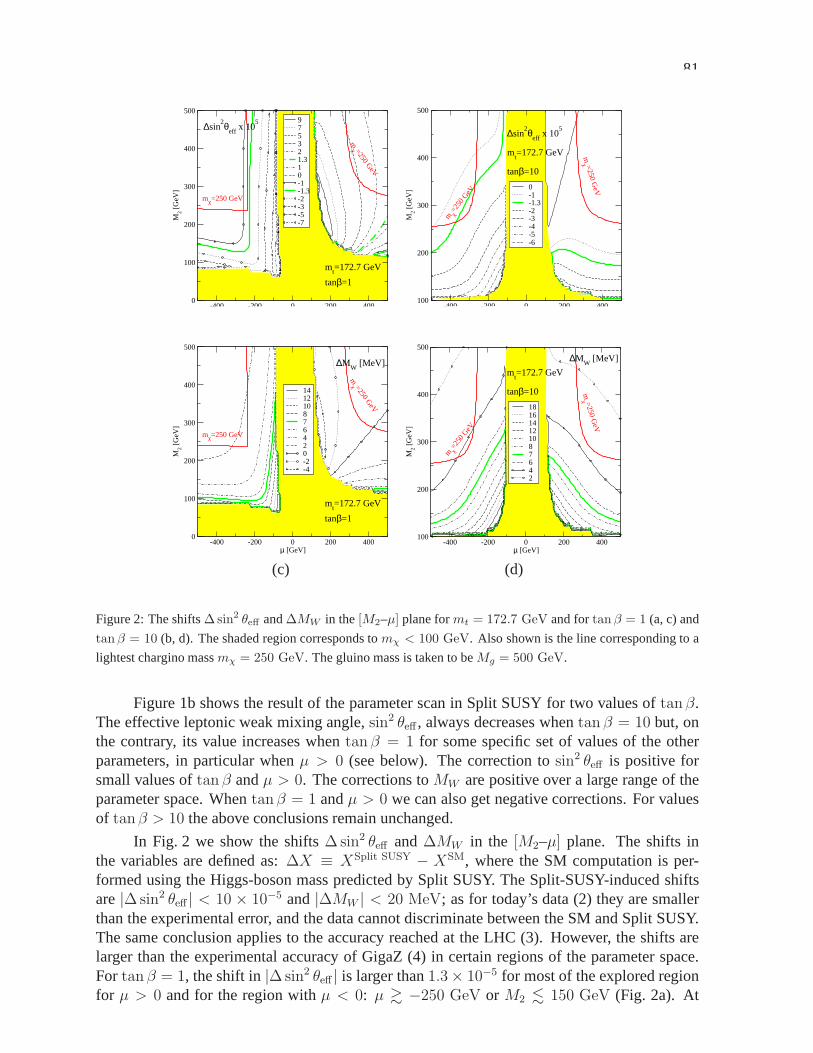
81

-400 -200 0 200 400µ [GeV]

0

100

200

300

400

500

M2 [G

eV]

∆sin2θ

eff x 10

5

mt=172.7 GeV

tanβ=1

mχ=250 GeV

mχ =250 G

eV

975321.310-1-1.3-2-3-5-7

-400 -200 0 200 400µ [GeV]

100

200

300

400

500

M2 [G

eV]

∆sin2θ

eff x 10

5

mt=172.7 GeV

tanβ=10

m χ=2

50 G

eV

mχ =250 G

eV

0-1-1.3-2-3-4-5-6

(a) (b)

-400 -200 0 200 400µ [GeV]

0

100

200

300

400

500

M2 [G

eV]

∆MW

[MeV]

mt=172.7 GeV

tanβ=1

mχ=250 GeV

mχ =250 G

eV

141210876420-2-4

-400 -200 0 200 400µ [GeV]

100

200

300

400

500

M2 [G

eV]

∆MW

[MeV]

mt=172.7 GeV

tanβ=10

m χ=2

50 G

eV

mχ =250 G

eV

181614121087642

(c) (d)

Figure 2: The shifts∆sin2 θeff and∆MW in the[M2–µ] plane formt = 172.7 GeV and fortanβ = 1 (a, c) and

tanβ = 10 (b, d). The shaded region corresponds tomχ < 100 GeV. Also shown is the line corresponding to a

lightest chargino massmχ = 250 GeV. The gluino mass is taken to beMg = 500 GeV.

Figure 1b shows the result of the parameter scan in Split SUSYfor two values oftanβ.The effective leptonic weak mixing angle,sin2 θeff , always decreases whentan β = 10 but, onthe contrary, its value increases whentan β = 1 for some specific set of values of the otherparameters, in particular whenµ > 0 (see below). The correction tosin2 θeff is positive forsmall values oftan β andµ > 0. The corrections toMW are positive over a large range of theparameter space. Whentanβ = 1 andµ > 0 we can also get negative corrections. For valuesof tanβ > 10 the above conclusions remain unchanged.

In Fig. 2 we show the shifts∆ sin2 θeff and∆MW in the [M2–µ] plane. The shifts inthe variables are defined as:∆X ≡ XSplit SUSY − XSM, where the SM computation is per-formed using the Higgs-boson mass predicted by Split SUSY. The Split-SUSY-induced shiftsare|∆ sin2 θeff | < 10 × 10−5 and|∆MW | < 20 MeV; as for today’s data (2) they are smallerthan the experimental error, and the data cannot discriminate between the SM and Split SUSY.The same conclusion applies to the accuracy reached at the LHC (3). However, the shifts arelarger than the experimental accuracy of GigaZ (4) in certain regions of the parameter space.For tan β = 1, the shift in|∆ sin2 θeff | is larger than1.3× 10−5 for most of the explored regionfor µ > 0 and for the region withµ < 0: µ & −250 GeV or M2 . 150 GeV (Fig. 2a). At

82

tan β = 10 (Fig. 2b),|∆ sin2 θeff | is larger than the future experimental accuracy (4) in a smallregionM2 . 175–200 GeV for µ > 0, and a large regionM2 . 200–500 GeV for µ < 0.As far asMW is concerned, the LHC measurement (3) could only be useful ina small cornerof the parameter space forµ < 0, tanβ >∼ 10. The GigaZ measurement (4) does not help fortan β = 1, µ > 0. For tan β = 1, µ < 0 there exists a small region forM2 . 110 GeV orµ > −110 GeV. For largertan β, the region of sensitivity is much larger. Summarizing theresults of Fig. 2:

• Positive shifts ofsin2 θeff are only possible at smalltanβ ≃ 1 andµ > 0. They are large,and correlated with small and negative shifts ofMW . These large shifts are possible evenfor large values of the chargino masses (mχ > 250 GeV).

• Fortan β ≃ 1, µ < 0 large negative shifts insin2 θeff are possible, correlated with positiveshifts inMW , butsin2 θeff is the most sensitive of those observables.

• For largetan β & 10 andµ > 0, the sensitivity region is confined to smallM2 . 275–375 GeV, with the largest shift provided bysin2 θeff for µ & 300 GeV, and byMW

otherwise.• Finally, for largetanβ & 10 andµ < 0, the largest sensitivity is provided bysin2 θeff ; it

can reach GigaZ sensitivities even for moderate chargino masses (mχ ≈ 250 GeV).

We would like to stress that the results for negativeµ are quite different from those of positiveµ. As Fig. 2 shows, changing the sign ofµ can change the sign and the absolute value of theshifts significantly.

The results of the difference between Split SUSY and SM predictions in theMW–sin2 θeffplane are displayed in Fig. 3, together with the expected error ellipses of the future colliders (3)and (4) centered at the SM value. We can see that the shift∆MW can be up to23 MeV atits maximum and it is impossible to discriminate between models at present. However, futureexperiments could be probed with the future precision onMW . On the other hand, the shifts∆ sin2 θeff can easily reach values±2 × 10−5, which is larger than both the expected experi-mental errors and the anticipated theoretical accuracies (5).

We observe from Fig. 1a that the current SM prediction ofMW–sin2 θeff would need apositive shift on both observables (together with a large value ofmt) to be closer to the centralexperimental value. Figs. 2, 3 show that the general trend ofthe Split SUSY contributionsis a negative correlation of the shifts on both observables.The region providing (∆MW > 0,∆ sin2 θeff > 0) is actually small and the largest region corresponds to (∆MW > 0, ∆ sin2 θeff <0) –c.f. Fig. 3. Of course, small deviations from the general trend are important, and Refs. [229,233] show that there are points of the parameter Split SUSY space that fit better than the SMthe experimental value of the electroweak precision observables.

4. CONCLUSIONS

We find that the shifts induced in Split SUSY models are smaller than present experimentalaccuracies (2), and no conclusion can be drawn with respect to the validity of this model. Withthe anticipated LHC accuracy onMW , a small corner of the parameter space can be explored.However, only with the GigaZ option of the ILC would the experiment be sensitive to theSplit SUSY corrections to these observables. In this option, the effective leptonic mixing angle(sin2 θeff) is the most sensitive of the two observables. For moderate and largetanβ, the lightestchargino must be relatively light,mχ . 250 GeV, and will already have been detected either atthe LHC or the ILC before the GigaZ era. The observables provide, however, a high-precision

83

Figure 3: Shifts of the differences between Split SUSY and SMpredictions forMW andsin2 θeff , scanning over

the parameter space. Also shown are the ellipses for the prospective accuracies at LHC/ILC (large ellipse) and

GigaZ (small ellipse).

test of the model. An interesting case is a scenario with lowtan β ≃ 1 and positiveµ, wherelarge shifts insin2 θeff are expected, even for large values of the chargino masses.

Acknowledgements

The work of S.P. has been supported by the European Union under contract No. MEIF-CT-2003-500030, and that of J.G. by aRamon y Cajalcontract from MEC (Spain) and in partby MEC and FEDER under project 2004-04582-C02-01 and Generalitat de Catalunya project2005SGR00564. S.P. is thankful for the warm hospitality at Les Houches 2005.

84

Part 11

Split supersymmetry with Dirac gauginomassesK. Benakli

AbstractWe consider a scenario where supersymmetry is broken by a slight de-formation of brane intersections angles in models where thegauge sec-tor arises in multiplets of extended supersymmetry, while matter statesare in N=1 representations. It leads to split extended supersymmetrymodels which can prvide the minimal particle content at TeV energiesto have both perfect one-loop unification and a good dark matter candi-date.

1. INTRODUCTION

Our knowledge of physics at energies above the electroweak scale leaves the door open to differ-ent ideas (extra-dimensions, compositeness...). The onlyconstraints come on the LEP precisionmeasurements and mathematicla consistency. Fortunately,there are a few observations whichcan serve as guidelines for building extensions to the Standard Model (SM), as the necessity ofa Dark Matter (DM) candidate and the fact that LEP data favor the unification of the three gaugecouplings. Both find natural realization in specific supersymmetric models as the Minimal Su-persymetric Standard Model (MSSM). Supersymmetry is also welcome as it naturally arises instring theory, which provides a framework for incorporating the gravitational interaction in ourquantum picture of the universe.

The failure to find a dynamical explanation of the very tiny dark energy in the universe,as indicated by recent observations, raises questions on our understanding of the notion of“naturalness”. It raises the possibility that even the gauge hierarchy problem is not solved by asymmetry. Supersymmetry could be present at very high energies and its breaking could leadto a hierarchy between the masses of the different superpartners such as in the so-called splitsupersymmetry scenario [222,223]. One of its imprtant features is that even making squarks andsleptons heavy, it is possible to keep successful unification and the existence of a DM candidate.Moreover, constraints related to its complicated scalar sector disappear.

Implementing this idea in string theory has been discussed in [265]. In this work we showthat there is an economical string-inspired brane models that allows for unification of gaugecouplings at scales safe from proton decay problems and provides us with a natural dark mattercandidate.

This work is based on [266].

2. MAIN FEATURES OF THE MODEL

The starting point of the construction is a supersymmetric extension of the standard model. Thisdiffers from the minimal extension (MSSM) and is as follows:

85

• Gauge bosons arise inN = 2 orN = 4 supermultiplets which are decomposed, for eachgauge group factorGa, into oneN = 1 vector superfieldWa and one or three chiraladjoint superfieldsAa, respectively.

• Quarks and leptons belong toN = 1 chiral multiplets.• Pairs of Higgs doublets originate asN = 1 chiral multiplets for light Binos Dirac masses

and inN = 2 supersymmetry hypermultiplets otherwise, as we will explain below.

These features have a natural realization in brane constructions: Gauge bosons emergeas massless modes living on the bulk of a stack of coincident branes. Quarks and leptons areidentified with massless modes localized at point-like brane intersections. The Higgs doubletsare localized in two tori where branes intersect, while theypropagate freely in the third toruswhere the two brane stacks are parallel.

We will asume that supersymmetry is broken by aD-term. This is achieved in the braneconstruction through deforming brane intersections with asmall angleΘ leading to theD-term〈D〉 = ΘM2

S associated to a corresponding magnetizedU(1) factor with superfield strengthW(see for example [267]). Here,MS is the string scale. This results in soft masses:

• A tree-level massm0 ∝√

ΘMS for squarks and sleptons localized at the deformed in-tersections. All other scalars acquire in general high masses of orderm0 by one loopradiative corrections. However an appropriate fine-tuningis needed in the Higgs sector tokeepnH doublets light.

• A Dirac mass [268] is induced through the dimension-five operator,

a

MS

∫

d2θWW aAa ⇒ mD1/2 ∼ a

m20

MS

, (1)

wherea accounts for a possible loop factor.

Actually, this operator (1) might not be present at tree-level and needs to be generatedthrough a loop diagram. In this case, we assume the existenceof a “messenger “ sector with thefollowing properties:

• The messenger states formN = 2 hypermultiplets with a supersymmetric massMX .• the scalars have massesM2

X ±m20 where the splitting is induced by the supersymmetry

breaking.

At one-loop a Dirac gaugino mass is induced:

mD1/2 ∼ α

MX

Ms× m2

0

Ms(2)

whereα is the corresponding gauge coupling. An explicit computation in string models givesat first order inm

20

M2s

[269]:

mD1/2 ∼ α

m20

Ms

∫ ∞

0

dt

t

∑

n

(

nR5Ms +MX

Ms

)

e−2πt(nR5Ms+MXMs

)2 (3)

where then = 0 sector reproduces the field theory results.

An important feature is that this mass does not breakR-symmetry and provides a way outto difficulties with generating gaugino masses for split supersymmetry models.

86

3. CONSTRAINTS FROM UNIFICATION

For the purpose of studying the unification of gauge couplings some simplifications are in order.First we assume equality of gluinos with winos massesmD

1/2 and we assume universality ofall scalar massm0, except fornH Higgs doublets that remain light at the electroweak scale.Moreover, we useMS ∼ MGUT and takea between1/100 ≤ a ≤ 1. Our results are given inTable 1.

nH a MGUT m0 mD1/2

N = 2 1 1 2.8 × 1018 4.5 × 1012 7.2 × 106

1 1/100 3.8 × 1018 3.2 × 1013 2.7 × 106

2 1 4.5 × 1016 1.1 × 1013 2.7 × 109

2 1/100 4.5 × 1016 8.6 × 1013 1.6 × 109

N = 4 1 1 9.7 × 1018 8.5 × 1015 7.4 × 1012

1 1/100 1019 6.8 × 1016 3.4 × 1012

2 — — —

Table 1: Values for the unification scaleMGUT , scalar massesm0 and Dirac gaugino massesmD1/2 in GeV for

N = 2, 4 supersymmetric gauge sector,nH = 1, 2 light Higgses, and varying the loop factora.

The results are always stable under the variation of the loopfactora. While the number ofparameters seems enough to always insure unification, the required values are not always real-istic and (perfect) one-loop unification is for instance notpossible forN = 4 andnh = 2. Thismight be achieved in refined analysis which would take into account different threshold cor-rections, as well as the contribution from the messenger sector described above, when present.In fact, these effects can be important for models with lowMX or with large compactificationvolume.

Nice features of the results are: (i) the unification scale lies at values which make themodel safe of problems with proton decay, (ii) fornH = 1 it is compatible with simultane-ous unification with gravitationnal interactions without resorting to unknown large thresholdcorrections.

4. CONSTRAINTS ON BINO MASSES FROM DARK MATTER

The masses of Binos are not constrained by unification requirements, but by the assumption thatthe neutralino provides an important fraction of the observed dark matter in the universe. Quasi-Dirac Higgsinos interact inelastically with matter via vector-like couplings and direct detectionexperiments put a lower bound on their mass of order 50 TeV. Pure higgsinos can not make agood dark matter.

A sizeable mixing with Binos must be introduced through the EW symmetry breaking.This is of orderm2

W/mD1/2 and implies an upper bound on the Dirac Bino mass of about105 GeV.

Only the case withN = 2, nH = 1 case is close to this value. For the other cases one needs a bigsupression factor is needed. One can play with the factorMX/Ms in (3), however in that case itis necessary to ensure that the messenger sector does not modify the unification results. This canbe achieved for instance if these states form complete representations ofSU(5). Moreover, theHiggs should be inN = 1 multiplets only in order to destroy the Dirac nature of the Higgsinomass.

We can instead ask that nomD1/2 is generated for Binos, but only for the other gauginos.

87

For instance, this is obtained when the messenger sector carry no hypercharge. In this case weuse instead Majorana masses generated at two-loop and corresponding to the dimension-seveneffective operator [270]:

b2

M3S

∫

d2θW2TrW 2 ⇒ mM1/2 ∼ b2

m40

M3S

, (4)

whereb is a loop factor. This givesmM1/2 ∼ 5 × 106 GeV for theN = 4 nH = 1 model and

mM1/2 ∼ 100 GeV for theN = 2 nH = 2 model. For theN = 2 nH = 1 case,mM

1/2 ∼ 10 keV istoo small and a Bino Dirac mass is necessary.

5. HIGGSINOS AND NEUTRALINOS MASSES

In the cases withnH = 1 andN = 4 or N = 2, µ is an independent parameter. It can beassociated with the separation of the branes in the torus where they are parallel. The darkmatter candidate is mainly a Higgsino mixing with a much heavier Bino . The relic densityreproduces the actual WMAP results forµ ∼ 1.1 TeV.

Instead, for theN = 2 nH = 2 the Higgsinos are inN = 2 multiplets and the dimension-seven operator,

c

M3S

∫

d2θW2D2H1H2 ⇒ µ ∼ c

m40

M3S

, (5)

wherec is again a loop factor, induces the desired mass (of the same order asmM1/2 of Eq. (4)).

In fact, masses of this order can be shown to be induced at one-loop by the messenger sectorthrough explicit string computation in D-brane constructions [269]. Electroweak symmetrybreaking leads then to the neutralino mass matrix:

M 0 mzswcβ mzswsβ0 M −mzswsβ mzswcβ

mzswcβ −mzswsβ 0 −µmzswsβ mzswcβ −µ 0

in the basis(B1, B2, H1, H2) and whereM = mM1/2 stands for the Bino Majorana masses. The

mass matrix can be diagonalized to obtain:

mχ = 1/2[

(M + ǫ1µ) − ǫ2√

(M − ǫ1µ)2 + 4m2zs

2w

]

(6)

where the four neutralinos with different mass eigenvaluesare labeled byǫ1,2 = ±1.

As for [223], we distinguishe three cases:

• M ≪ µ: is exculded as the Bino does not interact strongly enough toannihilate andwould overclose the universe.

• M ≫ µ: WMAP data requireµ ∼ 1.1 TeV.• M ∼ µ: the lightest neutralino (χ), a mixture of Higgsinos and Binos, is candidate for

dark matter. It allows low values forµ.

Note that the models withnH = 1 have the minimal content at the electroweak scale toaddress both unification and dark matter problems. They differ from [271] as we can achieveperfect unification even at one-loop, and at scales high enough to keep the model safe from fastproton decay.

88

It is possible to check that the life time of the extra states does not further constrain thesemodels. This is easy for the case ofN = 2. There, scalars can decay into gauginos, Diracgluinos decay through squark loops sufficiently fast and Dirac Winos and Binos decay intoHiggses and Higgsinos. Generically only one of thr two Majorana Binos couples to matter, theother remains stable. To avoid this, it was essensial that Higgses arise inN = 2 hypermultipletsgiving rise to the mass matrix (5.). The only stable particleis the usual lightest sparticle (LSP).In theN = 4 model, scalars still decay into gauginos, but we have nowtwo Dirac gluinos,Winos and Binos. Whiloe half of them decay as before, either through scalar loops or intoHiggs-Higgsinos, the other half can only decay through string massive states. Their lifetimeis then estimated byτ ∼ (MS/1013 GeV)

4(102 GeV/mg)

5τU , wheremg is the gaugino mass

andτU is the lifetime of the universe. For gluinos and Winos there is no problem, but Binos arevery long lived although still safe, with a life-time of order τU/10.

6. SOME REMARKS ON THE COLLIDER PHENOMENOLOGY

The signatures at future colliders can be discussed either as a function of the model parameters(M,µ), or as a function of the low energy observables(mχ±,∆mχ).

First, thenH = 1 scenario:µ ∼ 1.1 TeV so the new states will be hardly observableat LHC. An e+e− Collider with center of mass energy of around 2.5 TeV will allow to detecta possible signature. Next, thenH = 2 scenario, the main collider signature is through theproduction of charginos. Their mass is given bymχ± = µ + δµ, whereδµ ∼ α

πµ is due to

electromagnetic contributions and is of order300 to 400 MeV. The produced charginos willdecay into the neutralino, mainly through emission of a virtualW± which gives rise to leptonpairs or pions depending on its energy. This decay is governed by the mass difference∆mχ =mχ± −mχ0 . Because charginos are produced through EW processes, LHC will mainly be ableto explore the case of very light charginos, which exist onlyin the limited area of the parameterspace withM ∼ µ. Unlike in low energy supersymmetry, the absence of cascadedecays inthis case will make it difficult to separate the signal from similar events produced by StandardModelW± production processes.

Let us discus the case ofe+e− colliders. For most of the(M,µ) parameter range,∆mχ

is small, at most of order a few GeV. Because the value ofδµ is not small enough to make thechargino long-lived as to produce visible tracks in the vertex detectors, we have to rely on itsdecay products. The produced leptons or pions are very soft and it would typically be difficult todisentangle them from the background due to emission of photons from the beam. The strategyis then to look fore+e− → γ + ET/ . A proper cut on the transverse momentum of the photonallows to eliminate the background of missing energy due to emission ofe+e− pairs along thebeam, as the conservation of transverse momentum implies now a simultaneous detection ofelectrons or positrons [272]. The best possible scenario iswhenM andµ are of the same ordersince, as soon asM starts to be greater thanµ, the Binos quickly decouple and this modelconverges to thenH = 1 scenario withµ ∼ 1.1 TeV.

With LEP precision measurements, a new era has opened up in the physics beyond theStandard Model. While still waiting for more experimental data, critics have been put forwardthe beauty of the “ MSSM with electroweak scale superpartners”, it has shaded and its abso-lute reign ended. New routes are being explored. If no symmetry or dynamical mechanismis invoked to solve the gauge hierarchy problem, then there is no reason today to expect thepresence of new signals at the TeV scale outside the Higgs bosons. Our motivation here forsupersymmetry is a top-down approach: we assume that it is a symmetry of the fundamental

89

theory in the ultraviolet. We are then tempted to analyze thedifferent routes for its breakingand if they have any phenomenological consequences. This (probably impossible) task is verymuch simplified if one requires from the theory to contain a dark matter candidate, to predictunification of couplings, and to show (approximative) universality of masses as was illustratedhere.

We studied a scenario where supersymmetry is broken throughsmall deformations ofintersecting brane angles. Sizable gaugino masses are difficult to generate in these modelsdue to the samllness of R-symmetry breaking. We circumvent this difficulty by considering asplit supersymmetry framework with Dirac masses for gauginos. Our results show that we caneasily obtain interesting models with the minimal content at the electroweak scale to addressboth unification and dark matter problems.

Acknowledgements

This work was supported in part by RTN contract MRTN-CT-2004-503369, in part by CICYT,Spain, under contracts FPA2001-1806 and FPA2002-00748, inpart by the INTAS contract 03-51-6346 and in part by IN2P3-CICYT under contract Pth 03-1.

90

Part 12

A search for gluino decays into a b quarkpair and a dilepton at the LHCT. Millet and S. Muanza

AbstractWe present a search at the LHC for gluinos undergoing the followingcascade decay:g → b1b → bbχ0

2 → bb + ℓ+ℓ− + χ01. In this first step

of this study, we focus on the signal properties and mass reconstruction.Results are given for 10 fb−1 of integrated luminosity at the LHC.

1. INTRODUCTION

This letter is devoted to the study of the following gluino cascade decay at the LHC:g → b1b→bbχ0

2 → bb+ ℓ+ℓ− + χ01. Our signal is defined as follows: the production process envisaged is:

pp→ qg and the squark decay channel considered is:q → q + χ01.

We expect a double advantage from the later choice. On one hand this process has a sufficientlylarge leading order (LO) cross section since it is proportional toα2

S. On the other hand theq → q + χ0

1 decay can have a large branching ratio and give a clean signature in theq decayhemisphere.

This leads to a complex topology with a hard and isolated jet from the squark decay on topof the rich gluino decay yielding 2 b-jets, a clean dilepton and large missing transverse energy( /ET ).

We aimed at reconstructing the gluino cascade decay in two steps: first for the signal alone,secondly including the background of both the Standard Model processes and the SUSY pro-cesses. To goal is to evaluate on this more realistic approach degrades the measure of sparticlemass differences that we can derive from this signal. We’ll essentially concentrate on the signalreconstruction in this first step of the study.

We produced Monte Carlo samples of the signal and backgroundprocesses using the Pythia6.325 [17] event generator. The later is interfaced to the LHAPDF 4.2 [273] and the TAUOLA2.6 [274] programs. These provide respectively the proton parton density functions and anaccurate description of tau decays and polarization. We performed a fast simulation the ATLASdetector response using ATLFAST [18].

Section 2 describes the signal properties. Section 3 details the online and offline event selection.The sparticle mass reconstruction is presented at section 4.

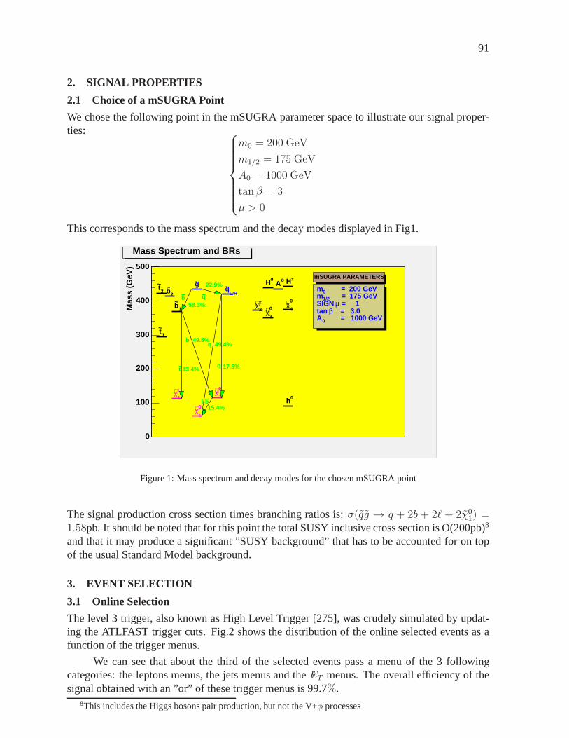
91

2. SIGNAL PROPERTIES

2.1 Choice of a mSUGRA Point

We chose the following point in the mSUGRA parameter space toillustrate our signal proper-ties:

m0 = 200 GeV

m1/2 = 175 GeV

A0 = 1000 GeV

tan β = 3

µ > 0

This corresponds to the mass spectrum and the decay modes displayed in Fig1.

Mas

s (G

eV)

0

100

200

300

400

500mSUGRA PARAMETERS

= 200 GeV0m = 175 GeV1/2m

= 1µSIGN = 3.0βtan

= 1000 GeV0A

g~

L/Rq~

0h

0A0H

±H

1t~

2t~

1b~2b~

0

1χ∼

0

2χ∼±

1χ∼

0

3χ∼

0

4χ∼±

2χ∼

22.9%

q58.3%

b

49.5%b

43.4%t

49.4%q

17.5%q

15.4%bb

Mass Spectrum and BRs

Figure 1: Mass spectrum and decay modes for the chosen mSUGRApoint

The signal production cross section times branching ratiosis: σ(qg → q + 2b + 2ℓ + 2χ01) =

1.58pb. It should be noted that for this point the total SUSY inclusive cross section is O(200pb)8

and that it may produce a significant ”SUSY background” that has to be accounted for on topof the usual Standard Model background.

3. EVENT SELECTION

3.1 Online Selection

The level 3 trigger, also known as High Level Trigger [275], was crudely simulated by updat-ing the ATLFAST trigger cuts. Fig.2 shows the distribution of the online selected events as afunction of the trigger menus.

We can see that about the third of the selected events pass a menu of the 3 followingcategories: the leptons menus, the jets menus and the /ET menus. The overall efficiency of thesignal obtained with an ”or” of these trigger menus is 99.7%.

8This includes the Higgs bosons pair production, but not the V+φ processes

92

Figure 2: The different trigger menus used for the online selection

3.2 Preselection

The preselection aims at rejecting most of the QCD background whilst keeping the highestsignal efficiency. The cuts applied at this level define the studied topology. They are obviouslydefined as additional requirements with respect to the online selection and defined as follows:

exactly 2 isolated leptons (with opposite signs and same flavor)

pT(e±) > 5 GeV, pT(µ±) > 6 GeV

|η(ℓ±)| < 2.5

at least 3 jets

pT (jets) > 10 GeV

|η(jets)| < 5.0

/ET > 100 GeV

Fig.3 shows the total number of reconstructed jets (left) aswell as the number of b-tagged jets.For the later an efficiency of 60% was used for jet actually coming from a b quark fragmentationwhereas a rejection factor of about 7 and 100 was used for jet from c quarks and light flavorquarks respectively. These values, as well as correction factors depending on the jetpT aretaken from the ATLFAST-B program. The signal efficiency after applying these preselectioncuts is:ǫ(signal) = 49.3%.

3.3 Double-Tag Analysis

Though it’s in principle possible to perform this signal search requiring only 1 b-tagged jet in theevents, we directly required 2 b-tagged jets in order to facilitate the jets combinatorics betweenthe squark and the gluino hemispheres. Therefore we used thesimple strategy of assigning

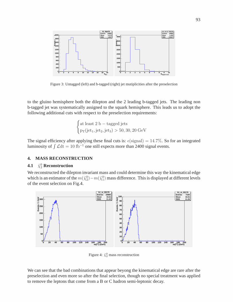
93

h1_Njet79Entries 24965Mean 5.574RMS 1.967

jetsN0 2 4 6 8 10 12 14 16 18 20

Eve

nts

/

1

0

200

400

600

800

1000

1200

1400

1600

1800

2000

h1_Njet79Entries 24965Mean 5.574RMS 1.967

h1_N_B_TAG79Entries 24965Mean 2.426RMS 0.9427

tagged b-jetsN0 1 2 3 4 5 6 7 8 9 10

Eve

nts

/

1

0

500

1000

1500

2000

2500

3000

3500

4000

h1_N_B_TAG79Entries 24965Mean 2.426RMS 0.9427

Figure 3: Untagged (left) and b-tagged (right) jet mutiplicities after the preselection

to the gluino hemisphere both the dilepton and the 2 leading b-tagged jets. The leading nonb-tagged jet was systematically assigned to the squark hemisphere. This leads us to adopt thefollowing additional cuts with respect to the preselectionrequirements:

at least 2 b − tagged jets

pT(jet1, jet2, jet3) > 50, 30, 20 GeV

The signal efficiency after applying these final cuts is:ǫ(signal) = 14.7%. So for an integratedluminosity of

∫Ldt = 10 fb−1 one still expects more than 2400 signal events.

4. MASS RECONSTRUCTION

4.1 χ02 Reconstruction

We reconstructed the dilepton invariant mass and could determine this way the kinematical edgewhich is an estimator of them(χ0

2)−m(χ01) mass difference. This is displayed at different levels

of the event selection on Fig.4.

h1_m_l0l179Entries 24965Mean 33.61RMS 11.42

) (GeV)-l+m(l0 20 40 60 80 100 120 140 160 180 200

Eve

nts

/ 1

GeV

0

50

100

150

200

250

300

h1_m_l0l179Entries 24965Mean 33.61RMS 11.42

h1_m_l0l179Entries 7194Mean 33.51RMS 11.26

) (GeV)-l+m(l0 20 40 60 80 100 120 140 160 180 200

Eve

nts

/ 1

GeV

0

10

20

30

40

50

60

70

80

90

100

h1_m_l0l179Entries 7194Mean 33.51RMS 11.26

Figure 4:χ02 mass reconstruction

We can see that the bad combinations that appear beyong the kinematical edge are rare after thepreselection and even more so after the final selection, though no special treatment was appliedto remove the leptons that come from a B or C hadron semi-leptonic decay.

94

One notes that the kinematical edge points near the expectedvalue of 54 GeV for our signalpoint. No fits and no uncertainty estimates on the actual value derived from this histogram aremade so far.

4.2 b1 Reconstruction

We reconstructed them(b1) −m(χ01) mass difference by calculating the 3-body invariant mass

of the dilepton and one of the 2 leading b-tagged jets. There are obviously wrong combinationsthat enter the distribution in Fig.5. But we are exclusivelyinterested the largest value of the 2combinations where we indeed see a kinematical edge.

h1_MSBOTTOM279

Entries 14670Mean 185.8RMS 63.91

) (GeV)1

0χ∼)-m(1b~m(0 50 100 150 200 250 300 350 400

Eve

nts

/ 2

GeV

0

5

10

15

20

25

30

35

40h1_MSBOTTOM279

Entries 14670Mean 185.8RMS 63.91

Figure 5:b1 mass reconstruction

Again, one notes that the edge points near the expected valueof 309 GeV for our signal point.

4.3 g Reconstruction

Finally we reconstruct them(g) − m(χ01) mass difference by calculating the 4-body invariant

mass obtained with the dilepton and the 2 leading b-tagged jets.

There one sees that the edge points slightly higher than the expected value of 360 GeV for oursignal point.

5. CONCLUSIONS AND PROSPECTS

5.1 Conclusions

We have shown that thepp→ q + g → q + b1b → q + χ01 + bbχ0

2 → q + bb + ℓ+ℓ− + 2χ01 is a

quite interesting process to search for and to study at the LHC. By looking at the signal alone,it seems feasible to reconstruct the following mass differences using the classical kinematicaledges:m(χ0

2) −m(χ01),m(b1) −m(χ0

1) andm(g) −m(χ01).

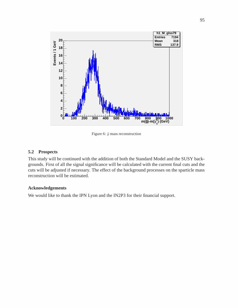
95

h1_M_glss79Entries 7194Mean 318RMS 137.9

) (GeV)1

0χ∼)-m(g~m(0 100 200 300 400 500 600 700 800 900 1000

Eve

nts

/ 1

GeV

0

2

4

6

8

10

12

14

16

18

20

h1_M_glss79Entries 7194Mean 318RMS 137.9

Figure 6:g mass reconstruction

5.2 Prospects

This study will be continued with the addition of both the Standard Model and the SUSY back-grounds. First of all the signal significance will be calculated with the current final cuts and thecuts will be adjusted if necessary. The effect of the background processes on the sparticle massreconstruction will be estimated.

Acknowledgements

We would like to thank the IPN Lyon and the IN2P3 for their financial support.

96

Part 13

Sensitivity of the LHC to CP violatingHiggs bosonsR.M. Godbole, D.J. Miller, S. Moretti and M.M. Muhlleitner

AbstractWe examine the sensitivity of the LHC to CP violation in the Higgs sec-tor. We show that for a Higgs boson heavy enough to decay into apair ofreal or virtualZ bosons, a study of the fermion pairs resulting from theZ/Z∗ decay, can provide a probe of possible CP non-conservation.Weinvestigate the expected invariant mass distribution and the azimuthalangular distribution of the process for a general Higgs-ZZ coupling.

1. INTRODUCTION

Whereas in the Standard Model (SM) CP violating effects are tiny, extensions of the SM, such as2-Higgs doublet models, exhibit new sources of CP violationwhich can lead to sizeable effectsin the Higgs sector [97, 276, 277]. In minimal supersymmetric theories, which are specificrealizations of 2-Higgs doublet models, two complex Higgs doublets have to be introduced toremove anomalies. After three of the Higgs doublet components have been absorbed to providemasses to the electroweak gauge bosons, the remaining five components give rise to a quintetof physical Higgs boson states. In a CP-conserving theory, besides two charged Higgs bosons,there are two CP-even neutral Higgs fields and one CP-odd neutral state. In case of CP violationin the Higgs sector the neutral Higgs bosons mix to give threeHiggs states with indefinite CPquantum numbers. While the prospects of establishing the CPquantum number of a spin 0state at the upcoming colliders are quite good, determination of the CP mixing, should the statehave an indefinite CP quantum number, is not very easy (See [278] for example for a recentsummary).

In this note we present observables which are sensitive to CPviolation in order to inves-tigate the sensitivity of the LHC to CP violation in the Higgssector. We then show preliminaryresults and give an outlook of the ongoing project.

2. THE DISTRIBUTIONS SENSITIVE TO CP VIOLATION

We exploit the Higgs decays toZ boson pairs to determine spin and parity of the Higgs boson.The Higgs boson is produced in gluon fusion at the LHC, and theZ bosons subsequently decayinto fermion pairs

gg → H → ZZ → (f1f1)(f2f2) (1)

This process includes cleanµ+µ− ande+e− decay channels for isolating the signal from thebackground and allowing a complete reconstruction of the kinematical configuration with goodprecision [279–281].

In Ref. [282] it has been shown that a model-independent analysis can be performedif supplemented by additional angular correlation effectsin gluon gluon fusion. To this end

97

helicity methods have been applied to generalize the Higgs coupling toZ bosons to arbitraryspin and parity. The most general vertex for a spin-0 Higgs boson in a CP non conserving theorycan then be written as

igMZ

cos θW[ agµν +

b

M2Z

pµpν + ic

M2Z

ǫµναβpαkβ ] (2)

with p = pZ1+ pZ2

, k = pZ1− pZ2

, pZ1andpZ2

being the four-momenta of the twoZ bosons,respectively, andθW denoting the electroweak mixing angle. The coefficientsa, b, c depend onthe theory, wherec 6= 0 is indicative of CP violation. The tree level Standard Modelcase isrecovered fora = 1 andb = c = 0. Note that this choice of vertex is gauge invariant for thisprocess. Any gauge dependence in theZ propagators is trivially cancelled when contractedwith the conserved lepton currents.

In the following we present the invariant mass distributionand the azimuthal angulardistribution of the Higgs decay width into twoZ bosons. The azimuthal angleφ is defined asthe angle between the planes of the fermion pairs stemming from theZ boson decays, cf. Fig. 1.

Figure 1: The definition of the polar anglesθi (i = 1, 2) and the azimuthal angleϕ for the sequential decay

H → Z(∗)Z → (f1f1)(f2f2) in the rest frame of the Higgs particle.

Fig. 2. left shows the invariant mass distribution for a Higgs boson of 150 GeV, decayinginto a pair of virtual and realZ bosons. We compare the distribution for a certain choice of theparametersa, b, c in the coupling given in Eq. (2) to the SM result. Fig. 2. rightpresents theazimuthal angular distribution for a Higgs particle of 280 GeV decaying in pair of realZ bosons,again compared to the Standard Model. As can be inferred fromthe figures, the distributionsshow a distinct behaviour for different models, encouraging further investigation of the angularobservables with respect to the sensitivity of the LHC to CP violation in the Higgs sector.

3. SENSITIVITY OF THE LHC TO CP VIOLATION

In order to get a first estimate of the sensitivity of the LHC toCP violation in the Higgs sectorthe cross section of the process given in Eq. (1) has been calculated for a Higgs boson massof 150 GeV as a function of the parametersb andc. The parametera has been chosen equalto the SM value,i.e. a = 1. For simplicity we choose the Higgs coupling to the gluons tobethe same as in the SM. The Higgs production cross section in gluon fusion has been calculatedwith the program HIGLU [283] which includes the QCD corrections at next-to-leading order.Again for simplicity, in the calculation of the branching ratio of the Higgs boson, we adopt the

98

Figure 2: The differential invariant mass distribution [left] and the azimuthal angular distribution [right] forMH =

150 GeV andMH = 280 GeV, respectively. The parameterization corresponds to the parameterization of the

HZZ vertex given in Eq. (2).

Figure 3: The sensitivity of the LHC to CP violation represented in the [b, c] plane fora = 1,MH = 150 GeV for

two different sensitivity criteria.

SM HWW coupling and only modify theHZZ coupling. Furthermore, it has been assumedthat the cuts applied to reduce the background alter the cross section in the same way as in theSM case,i.e. by about a factor 10 for an integrated luminosity of 100 fb−1 [279]. Since theATLAS study, where this number has been taken from, is done for a LO gluon fusion crosssection, the following results are presented for the LO production for reasons of consistency.NLO corrections would alter the production section by abouta factor 2 before cuts. In Fig. 3.we present the scatter plots in be[b, c] plane representing the points which fulfill the sensitivitycriteria we adopt. In order to have large enough significances (at least>∼5) the total cross sectionis required to be larger than 1.5 fb. Furthermore, the difference between the cross sectionincluding the general CP violatingHZZ coupling should differ from the SM cross section by

99

more than 1(5) fb. Our sensitivity criteria, forgg → H → Z∗Z∗ → (l+l−)(l+l−) , are

σb,c 6=0 > 1.5 fb (l = e, µ) (3)

|σb,c 6=0 − σSM| > 1(5) fb

Fig. 3. shows the sensitivity areas in the[b, c] plane according to the criteria Eq. (3) incase the difference to the SM result exceeds 1 fb (left) and 5 fb (right). In the former case thesensitivity area is almost covered by the LHC.

4. OUTLOOK

In the next step we will confront our results obtained for theLHC sensitivity with proposedCP violating models in the literature and we will refine the experimental side of the analy-sis. We will furthermore investigate to which extent the LHCwill be sensitive to CP violationin the various distributions presented in section 2. The analysis will as well be extended tothe most general case, i.e. to spin 1 and spin 2 particle couplings toZZ in order to be asmodel-independent as possible. The resulting programPHIZZ will be made available to theexperimental community for more detailed studies.

100

Part 14

Testing the scalar mass universality ofmSUGRA at the LHCS. Kraml, R. Lafaye, T. Plehn and D. Zerwas

AbstractWe investigate to which extent the universal boundary conditions ofmSUGRA can be tested in top-down fits at the LHC. Focusing in par-ticular on the scalar sector, we show that the GUT-scale soft-breakingmasses of the squarks are an order of magnitude less well constrainedthan those of the sleptons. Moreover, if the values ofmA andµ arenot known, the fit is insensitive to the mass-squared terms ofthe Higgsfields.

If supersymmetry is realised in nature, sparticle masses will be measured from measure-ments of kinematic endpoints [167,284] in cascade decays like qL → qχ0

2 → ql±l∓R → ql±l∓χ01

at the LHC. The optimal next step would then be to extract the SUSY breaking parameters atthe electroweak scale in a global fit and extrapolate them to the GUT scale [53,285] to test theirhigh-scale boundary conditions. A complete MSSM fit may, however, have too many parame-ters compared to the number of observables available at the LHC. This has been shown recentlyusing new fitting tools such as Fittino [53,54] and SFitter [56]. The alternative procedures willthen be to determine the underlying parameters either by fixing a sufficient number of parame-ters (those the least sensitive to the avaialable measurements) to a defined value or in top-downfits of particular models of SUSY breaking. Such top-down fits, see e.g. [284], are in fact quitepopular in benchmark studies within the minimal supergravity (mSUGRA) model, in which theSUSY-breaking gaugino, scalar and trilinear parametersm1/2, m0 andA0, respectively, eachobey universal boundary conditions at the GUT scale,

However, as we discuss in this contribution, care has to be taken not to draw too strongconclusions from just a mSUGRA fit. As a matter of fact, the determination of the commonscalar mass,m0, is dominated by the precise measurement of the endpoint of the l±l∓ invari-ant massmmax

ll —in other words by theχ01, χ

02 and lR mass differences. Kinematic endpoints

involving jets, which give the squark and gluino masses, aremeasured about an order of mag-nitude less precisely thanmmax

ll . Moreover, in the renormalization group running, the squarkmass parameters are driven bym1/2 with a large coefficient and are hence much less sensitivetom0 than the slepton masses:

m2L∼ m2

0 + 0.5m21/2 , m2

E∼ m2

0 + 0.15m21/2 , (1)

m2Q∼ m2

0 + 6.3m21/2 , m2

U,D∼ m2

0 + 5.8m21/2 . (2)

Additionally the error onm0 is proportional to the product of the error on sfermion mass andthe sfermion mass itself. Thus for a squark mass typically three times as large as a slepton mass,the relative experimental error on the squark mass measurement must be an order of magnitudemore precise than the measurement of the slepton mass to obtain the same sensitivity, which is

101

difficult to achieve. For these reasons, measurements of squarks have little influence on the fitof a universalm0.

While the assumption of a universalm0 simplifies the model a lot, there is no strong the-oretical basis for this. When embedded in a higher gauge group, sparticles which come in thesame multiplet have equal masses. This is for example the case for squarks and sleptons inSU(5) or SO(10) GUTs. Non-universal scalar masses are also heavily constrained by flavour-changing neutral currents (FCNC), at least for the first and second generation. However, theremay be non-universal D-terms and/or GUT-scale threshold corrections, and the FCNC con-straints are much less severe for the third generation. Lastbut not least, there is no sound theo-retical argument whatsoever for the universality of the mass-squared terms,m2

H1,2, of the Higgs

fields. (If it is given up,µ andmA become free parameters of the model.) For these reasons,and because of it’s important phenomenological implications, the assumption of scalar-massuniversality should be treated with caution.

In this contribution, we study the implications of relaxingthe scalar-mass universality ofmSUGRA in the top-down parameter determination. To this aim, we assume the perspectiveLHC edge measurements at SPS1a according to [75]. In general, several of the LHC measure-ments of SPS1a with an integrated luminsoity of 300 fb−1 are dominated by the systematic erroron the knowledge of the energy scale, which is 1% for jets and 0.1% for leptons (electrons andmuons). For the light Higgs mass,mh0, we assume an experimental error of 250 MeV and a the-oretical error of 3 GeV [156]. We then useSFITTER [55, 56] to determine the parameters fornon-universal SUGRA scenarios. The results are summarizedin Table 1.9 First, as a reminder,case A shows the results of a strict mSUGRA fit [55], which leads to aO(1%) accuracy onm0,m1/2 andtanβ, and∼ 20 GeV accuracy onA0. Note that as poited out in [55] the fit to the edgevariables gives a much better result than the fit to the extracted SUSY masses. Next, for case B,we have relaxed the universality between slepton, squark and Higgs mass parameters, treatingm0(l),m0(q) andm2

H = m2H1

= m2H2

as independent parameters. As expected, the scalar-massparameter of the squarks,m0(q), turns out to be an order of magnitude less well derterminedthan that of the sleptons,m0(l). The Higgs mass parameters have a very large∼ 100% errrorin this case. The precision ontanβ andA0 also degrades, fortan β by a factor of 1.6 and forA0 by a factor of 2.6 (from 21 GeV to 54 GeV). Finally, in case C we have assumed universalscalar masses for sleptons and squarks of the first two generations (l, q), but treated those of thethird generation and of the Higgs fields as free parameters. The resulting errors onm0(t, b) andm0(l, q) are more or less similar to case B, but that onm2

H becomes almost 200% andm0(τ ),relying almost only on theττ invariant mass edge measurement, remains undetermined. Alsothe error onA0 increases to 75 GeV.

We have also studied the influence of particular measurements on the fit. The measure-ment of the sbottom masses, for instance, is of course crucial for the determination ofm0(t, b).In addition, it also has an important impact on the determination of tan β andA0: without thesbottom measurement, the error ontan β increases by about a factor of 2 and that onA0 byabout a factor of 4 in cases B and C. The influence ofmh is small in these cases because of its3 GeV theoretical uncertainty. The pseudoscalar massmA, on the other hand, would have animportant influence. A measurement ofmA at the level of 10% would mainly improve the erroron tanβ. This is shown as case D in Table 1. In order to determinem2

H , one would need toobtain a better uncertainty on the Higgs masses and to know theµ parameter in addition.

9As the central values of the measurements were used, the value of theχ2min of the fit is zero by construction

and therefore not quoted.

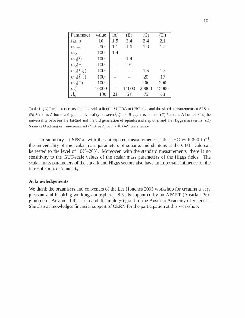
102

Parameter value (A) (B) (C) (D)tan β 10 1.5 2.4 2.4 2.1m1/2 250 1.1 1.6 1.3 1.3m0 100 1.4 – – –m0(l) 100 – 1.4 – –m0(q) 100 – 16 – –m0(l, q) 100 – – 1.5 1.5m0(t, b) 100 – – 20 17m0(τ) 100 – – 200 200m2H 10000 – 11000 20000 15000

A0 −100 21 54 75 63

Table 1: (A) Parameter errors obtained with a fit of mSUGRA to LHC edge and threshold measurements at SPS1a.

(B) Same as A but relaxing the universality betweenl, q and Higgs mass terms. (C) Same as A but relaxing the

universality between the 1st/2nd and the 3rd generation of squarks and sleptons, and the Higgs mass terms. (D)

Same as D addingmA measurement (400 GeV) with a 40 GeV uncertainty.

In summary, at SPS1a, with the anticipated measurements at the LHC with 300 fb−1,the universality of the scalar mass parameters of squarks and sleptons at the GUT scale canbe tested to the level of 10%–20%. Moreover, with the standard measurements, there is nosensitivity to the GUT-scale values of the scalar mass parameters of the Higgs fields. Thescalar-mass parameters of the squark and Higgs sectors alsohave an important influence on thefit results oftanβ andA0.

Acknowledgements

We thank the organisers and conveners of the Les Houches 2005workshop for creating a verypleasant and inspiring working atmosphere. S.K. is supported by an APART (Austrian Pro-gramme of Advanced Research and Technology) grant of the Austrian Academy of Sciences.She also acknowledges financial support of CERN for the participation at this workshop.

TOOLS

104

Part 15

A repository forbeyond-the-Standard-Model toolsP. Skands, P. Richardson, B. C. Allanach, H. Baer, G. Belanger, M. El Kacimi, U. Ellwanger,A. Freitas, N. Ghodbane, D. Goujdami, T. Hahn, S. Heinemeyer, J.-L. Kneur, G. Landsberg,J. S. Lee, M. Muhlleitner, T. Ohl, E. Perez, M. Peskin, A. Pilaftsis, T. Plehn, W. Porod, H. Przysiez-niak, A. Pukhov, D. Rainwater, J. Reuter, S. Schumann, S. Sherstnev, M. Spira and S. Tsuno

AbstractTo aid phenomenological studies of Beyond-the-Standard-Model (BSM)physics scenarios, a web repository for BSM calculational tools hasbeen created. We here present brief overviews of the relevant codes,ordered by topic as well as by alphabet. The online version ofthe repos-itory may be found at:http://www.ippp.dur.ac.uk/montecarlo/BSM/

1. INTRODUCTION

The physics programme at present and future colliders is aimed at a truly comprehensive ex-ploration of the TeV scale. On the theoretical side, recent years have seen the emergence of animpressive variety of proposals for what physics may be uncovered by these machines in justa few years. The ideas range from hypotheses of new fundamental matter (e.g. right-handedneutrinos) or forces (Z′ models), to new space-time symmetries (supersymmetry), oreven newspatial dimensions — at times with singularly spectacular consequences, such as the possibleproduction of microscopic black holes.

In the wake of many of these proposals, developments of computerised calculations ofmass spectra, couplings, and experimental observables, have taken place. For others, such toolsare yet to be created. Let it be stressed that this is not a point of only theoretical or phenomeno-logical interest. Experiments and analyses are not constructed purely with mechanical tools.Theoretical predictions, for expected signal strengths aswell as background levels, constitute acrucial part of the optimisation of both detectors, triggers, and analysis strategies. It is thereforeessential to have access to tools for calculating observables for as wide a range of phenomeno-logical signatures as possible.

The present brief overview and associated web repository aims to assess the present situa-tion and facilitate the information gathering process for people wishing to perform phenomeno-logical calculations in scenarios of physics beyond the Standard Model. We hope this may servealso to stimulate further work in the field. In Section 2., we first present a brief index of codesorganised by physics topic. Next, in Section 3., a full, alphabetical overview is given, describ-ing the contents of the repository at the time of writing. Other recent overviews of BSM-relatedphysics tools can be found in [286–289].

105

2. TOOLS BY PHYSICS TOPIC

This section is merely intended as an index, useful for finding out which tools exist for a givenphysics scenario. The main repository is then described in alphabetical order in the next section.

Supersymmetry

• CALCHEP: MSSM tree-level matrix element generator. Phase spaceintegration andevent generation. Extensions possible.

• COMPHEP: MSSM tree-level matrix element generator. Phase spaceintegration andevent generation. Extensions possible.

• CPSUPERH: Higgs phenomenology in the MSSM with explict CP Violation.• FEYNHIGGS: MSSM Higgs sector including explicit CP-violation (masses, couplings,

branching ratios, and cross sections).• HERWIG: Event generator for the MSSM (with and without RPV). Interface to ISAJET.• ILCSLEPTON: NLO cross-sections for slepton production ine+e− ande−e− collisions.• HDECAY: MSSM Higgs decay widths including loop effects.• ISAJET: MSSM event generator. MSSM mass and coupling spectrum, decay widths.

Checks against experimental constraints.• MICROMEGAS: MSSM (work on CPV in progress) and NMSSM dark matter relic den-

sity.• NMHDECAY: NMSSM mass spectrum plus couplings and decay widths of all Higgs

bosons. Checks against experimental constraints.• O’M EGA: MSSM tree-level matrix element generator. Extensions possible.• PROSPINO: SUSY-NLO cross sections at hadron colliders.• PYTHIA : MSSM event generator. RPV decays. Extensions to R-hadronsand NMSSM

available.• SDECAY: MSSM decay widths including loop effects.• SHERPA: MSSM event generator.• SOFTSUSY: MSSM mass and coupling spectrum.• SPHENO: MSSM mass and coupling spectrum, decay widths, ande+e− cross sections.• SUSPECT: MSSM mass and coupling spectrum.• SUSY-MADGRAPH: MSSM Matrix Elements.• SUSYGEN3: MSSM event generator (with and without RPV).

Extra Dimensions

• CHARYBDIS: Black hole production in hadron-hadron collisions.• HERWIG: Resonant graviton production in hadron-hadron collisions.• MICROMEGAS: Dark matter relic density. UED and warped extra dimensionsbeing

implemented.• PANDORA/PANDORA-PYTHIA : ADD extra dimensions. Work in progress: UED.• PYTHIA : RS graviton excitations.• PYTHIA UED: Universal Extra Dimensions.• SHERPA: ADD extra dimensions.

106

• TRUENOIR: Black hole production.

Extra Gauge Bosons,Z′/W′ models.

• PANDORA/PANDORA-PYTHIA : Z′ models.• PYTHIA : Z′ andW′ models.

Other Exotics

• O’M EGA: Anomalous triple and quartic gauge couplings. Extensionspossible.• [email protected]: Leptoquark event generator forpp andpp collisions.• PYTHIA : Technicolor, doubly charged Higgs bosons, excited fermions, anomalous cou-

plings, leptoquarks, fourth generation fermions.

3. TOOLS BY ALPHABET

We here give a detailed alphabetical list of the tools present in the repository at the time theseproceedings went to press. Note that the preceding section contains a useful list of tools bytopic, i.e. which tools are relevant for extra dimensions, which ones for Z’ etc.

CalcHEP

Contact Person:A. Pukhov,[email protected]

Web Page:http://theory.sinp.msu.ru/ ∼pukhov/calchep.html

CALCHEP is a program for symbolic calculation of matrix elementsand generation of C-codesfor subsequent numerical calculations. The model has to be defined in tems of lists of vari-ables, constraints, particles and list of vertices. Various BSM can be implemented and inves-tigated. In partiqular CALCHEP links to SUSPECT, ISAJET, SOFTSUSY, and SPHENO forMSSM. It also contains a Monte Carlo generator for unweighted events and a simple programwhich passes these events to PYTHIA . CALCHEP is a menu driven system with context helpfacility and is accompanied by a manual. At the same time CALCHEP can be used in thenon-interactive regime as a generator of matrix elements for other programs. In this mode itis implemented inMICROMEGAS for automatic generation of matrix elements of annihilationand co-annihilation of super-particles. Restrictions: tree level matrix elements, not more than 6particles in initial/final states. The last restriction is caused by modern computer facilities andby the implemented method of calculation (squared amplitudes). But for calculation of separatediagrams it was successfuly used for 2→5 and 2→6 processes.

Charybdis

Contact Person:P. Richardson,[email protected]

Web Page:www.ippp.dur.ac.uk/montecarlo/leshouches/generators /charybdis/

Charybdis simulates black hole production in hadron-hadron collisions using a geometric ap-proximation for the cross section together with Hawking evaporation of the black hole using thecorrect grey-body factors. It is described in more detail in[290].

107

CompHEP

Contact Person:Sasha Sherstnev,[email protected]

Web Page:http://theory.sinp.msu.ru/comphep

The COMPHEP package was created for calculation of multiparticle final states in collisionand decay processes. The main idea in COMPHEP was to enable one to go directly from thelagrangian to the cross sections and distributions effectively, with the high level of automation.The officially supported models are SM (in two gauges), unconstrained MSSM (in two gauges),MSSM with SUGRA and Gauge-Mediated SUSY breacking machanisms. The special programLANHEP allows new BSM models to be implemented to COMPHEP.

CPsuperH

Contact Persons:J. S. Lee,[email protected]

A. Pilaftsis,[email protected] Page:http://www.hep.man.ac.uk/u/jslee/CPsuperH.html

CPSUPERH [97] is a newly-developed computational package that calculates the mass spec-trum, couplings and branching ratios of the neutral and charged Higgs bosons in the MinimalSupersymmetric Standard Model with explicit CP violation [93, 291–294]. The program isbased on recent renormalization-group-improved diagrammatic calculations that include dom-inant higher-order logarithmic and threshold corrections, b-quark Yukawa-coupling resumma-tion effects and Higgs-boson pole-mass shifts [295–299].

The code CPSUPERH is self-contained (with all subroutines included), is easy and fast torun, and is organized to allow further theoretical developments to be easily implemented. Thefact that the masses and couplings of the charged and neutralHiggs bosons are computed at asimilar high-precision level makes it an attractive tool for Tevatron, LHC and LC studies, alsoin the CP-conserving case.

FeynHiggs

Contact Person:T. Hahn,[email protected]

S. Heinemeyer,[email protected]

Web Page:http://www.feynhiggs.de

FeynHiggs is a program for computing MSSM Higgs-boson masses and related observables,such as mixing angles, branching ratios, couplings and production cross sections, includingstate-of-the-art higher-order contributions (also for the case of explicit CP-violation). The cen-terpiece is a Fortran library for use with Fortran and C/C++.Alternatively, FeynHiggs has acommand-line, Mathematica, and Web interface. The command-line interface can process, be-sides its native format, files in SUSY Les Houches Accord format. FeynHiggs is an open-sourceprogram and easy to install. A web-based interface is available atwww.feynhiggs.de/fhucc .For further information, see also [74,155,156,277,300].

[email protected]

Contact Person:S. Tsuno,[email protected]

Web Page:http://atlas.kek.jp/physics/nlo-wg/index.html

GR@PPA event generator for Leptoquark model. The code generates unweighted events forscalar or vector type Leptoquark models. The Leptoquarks are generated, and decayed into

108

quark and lepton(neutrino) so that the decay properties of the final particles are correctly han-dled. In the vector Leptoquark production, two anomalous couplings are included in the in-teraction vertices. The decay mode depends on the model induced in the unified theory. Theprogram thus keeps flexibility for the Leptoquark decay. Thedetails description can be foundon the web page, where also the model file which contains the Leptoquark interaction for theGRACE system is available.

HDecay

Contact Person:M. Spira,[email protected]

Web Page:http://people.web.psi.ch/spira/hdecay/

HDECAY [301] calculates the branching ratios and total widths of SMand MSSM Higgsbosons.

Herwig

Contact Person:P. Richardson,[email protected]

Web Page:http://hepwww.rl.ac.uk/theory/seymour/herwig/

HERWIG [11] is a general purpose event generator for the simulationof Hadron Emission Re-actions With Interfering Gluons. The main concentration ison the simulation of the StandardModel although SUSY (with and without RPV [302]) is implemented together with resonantgravition production in hadron-hadron collisions.

ILCslepton

Contact Person:A. Freitas,[email protected]

Web Page:http://theory.fnal.gov/people/freitas/

The programs calculate the complete electroweak one-loop corrections to slepton production ine+e− ande−e− collisions (i.e. at ILC). Besides the virtual loop corrections, real photon radia-tion is included in order to provide a finite and well-defined result. For the sake of consistentrenormalization, the programs take the MSSM soft breaking parameters at an arbritary scaleas input; it is not possible to use masses and mixing angles asinput parameters. The availablecodes allow the computation of the total and angular differential cross-sections for selectron,smuon and sneutrino production. For more information, see [303,304].

Isajet

Contact Person:H. Baer,[email protected]

Web Page:http://www.phy.bnl.gov/ ∼isajet/

Simulatespp, pp, ande+e− interactions at high energies. Calculates SUSY and Higgs spectrumalong with SUSY and Higgs 2 and 3 body decay branching fractions. Evaluates neutralino relicdensity, neutralino-nucleon scattering cross sections,Br(b → sγ), (g− 2)µ, Br(Bs− > µ+µ−).

micrOMEGAs

Contact Persons:G. Belanger, F. Boudjema, A. Pukhov, A. Semenov,[email protected]

Web Page:http://lappweb.in2p3.fr/lapth/micromegas/index.html

109

MICROMEGAS is a code that calculates the relic density of the dark matterin supersymmetry.All annihilation and coannihilation processes are included. The cross-sections, extracted fromCALCHEP, are calculated exactly using loop-corrected masses and mixings as specified inthe SUSY Les Houches Accord. Relativistic formulae for the thermal average are used andcare is taken to handle poles and thresholds by adopting specific integration routines. In theMSSM, the input parameters can be either the soft SUSY parameters or the parameters of aSUGRA model specified at the GUT scale. In the latter case, a link with SUSPECT, SOFTSUSY,SPHENOand ISAJETallows to calculate the supersymmetric spectrum, Higgs masses, as well asmixing matrices. Higher-order corrections to Higgs couplings to quark pairs including QCD aswell as some SUSY corrections are implemented. Cross-sections for any 2→2 process as wellas partial decay widths for two-body final states are provided. Cross-sections for neutralinoannihilation at v∼0, relevant for indirect detection of neutralinos, are automatically computed.In the MSSM, routines calculating(g − 2)µ, Br(b → sγ), Br(Bs → µ+µ−) are also included.MICROMEGAS can be extended to other models by specifying the corresponding model file inthe CALCHEP notation.

NMHDecay

Contact Person:U. Ellwanger,[email protected]

Web Page:http://www.th.u-psud.fr/NMHDECAY/nmhdecay.html

The Fortran code NMHDECAY computes the sparticle masses and masses, couplings and decaywidths of all Higgs bosons of the NMSSM in terms of its parameters at the electroweak (SUSYbreaking) scale: the Yukawa couplingsλ andκ, the soft trilinear termsAλ andAκ, andtan(β)andµeff = λ < S >. The computation of the Higgs spectrum includes the leadingtwo loopterms, electroweak corrections and propagator corrections. Each point in parameter space ischecked against negative Higgs bosons searches at LEP, including unconventional channelsrelevant for the NMSSM. A link to a NMSSM version of MICROMEGAS allows to computethe dark matter relic density, and a rough (lowest order) calculation of the BR(b → sγ) isperfromed. One version of the program uses generalized SLHAconventions for input andoutput. For further information, see also [218,305].

O’Mega

Contact Person:T. Ohl,[email protected]

J. Reuter,[email protected] Page:http://theorie.physik.uni-wuerzburg.de/ ∼ohl/omega/

O’Mega constructs [306] optimally factorized tree-level scattering amplitudes (starting from2→4 processes, the expressions are much more compact and numerically stable than naivesums of Feynman diagrams). Officially supported models are the Standard Model and the com-plete MSSM (since version 0.10, of November 2005). Users canadd new interactions (e.g.anomalous triple and quartic gauge couplings are part of thedistributed version).

Complete automatized event generation for the LHC and the ILC is possible in concertwith WHiZard.

Pandora

Contact Person:M. Peskin,[email protected]

110

Web Page:http://www-sldnt.slac.stanford.edu/nld/new/

Docs/Generators/PANDORA.htm

Pandora is a parton-level physics simulation fore+e− linear colliders, including polarizationand beam effects. Pandora comes with an interface, Pandora-Pythia, that hadronizes events withPythia and decays polarized taus with tauola. The current distribution (Pandora 2.3) includes animplementation of the ADD extra dimension model (e+e− → γG and virtual graviton exchangein e+e− → f f, W+W−, ZZ, γγ), and a two-parameterZ′ model. We are currently working oninclusion of more generalZ′ models and inclusion of UED production and decay.

Prospino

Contact Person:T. Plehn,[email protected]

Web Page:http://pheno.physics.wisc.edu/ ∼plehn

For most applications the uncertainty in the normalizationof Monte Carlos for the production oftwo supersymmetric particles is large. The reason are largeSUSY and SUSY-QCD correctionsto the cross section. Prospino2 is the tool you can to use to normalize your total rates. Somedistributions are available on request. For detailed information on the production processesincluded, on papers available for more information, and on downloading and running the code,please see the web pages.

Pythia

Contact Person:P. Skands,[email protected]

Web Page:http://www.thep.lu.se/ ∼torbjorn/Pythia.html

In the context of tools for extra dimensions, PYTHIA contains cross sections for the productionof Randall-Sundrum graviton excitations, with the parton showers corrected to RS+jet matrixelements for hard jet radiation [307]. PYTHIA can also be used for a number of other BSMphysics scenarios, such as Technicolor [308],Z′/W′ [309] (including interference withZ/γ andW bosons), Left–Right symmetry (Higgs triplets), leptoquarks, compositeness and anomalouscouplings (including excited quarks and leptons), and of course a large variety of SUSY signalsand scenarios (forR-hadrons see [310]; for RPV see [311, 312]; for the NMSSM see [313]).Interfaces to SLHA, ISAJET, and FEYNHIGGS are available. For further information, see thePYTHIA manual [46], Chapter 8, and the PYTHIA update notes, both available on the PYTHIA

web page.

Pythia UED

Contact Person:H. Przysiezniak,[email protected]

M. El KacimiD. Goujdami

Web Page:http://wwwlapp.in2p3.fr/ ∼przys/PythiaUED.html

A generator tool which uses PYTHIA to produce events in the UED (Universal Extra Dimen-sions) model of Appelquist, Cheng and Dobrescu [314], with one extra dimension and addi-tional gravity mediated decays [315].

SDecay

Contact Person:M. Muhlleitner,[email protected]

111

Web Page:http://lappweb.in2p3.fr/pg-nomin/muehlleitner/SDECA Y/

Calculates the 2- and 3-body decays and loop-induced decaysof the supersymmetric particlesincluding the QCD corrections to the decays involving coloured particles and the dominantelectroweak effects to all decay modes.

Sherpa

Contact Person:S. Schumann, F. Krauss,[email protected]

Web Page:http://www.sherpa-mc.de/

SHERPA [316] is a multi-purpose Monte Carlo event generator that isable to simulate high-energetic collisions at lepton and hadron colliders. The physics programme of SHERPA covers:1) The description of hard processes in the framework of the Standard Model, the MinimalSupersymmetric Standard Model and the ADD model of large extra dimensions using tree levelmatrix elements provided by its internal matrix element generator AMEGIC++ [317, 318]. 2)Multiple QCD bremsstrahlung from initial and final state partons. 3) The consistent merging ofmatrix elements and parton showers according to the CKKW prescription. 4) Jet fragmentationand hadronisation provided by an interface to PYTHIA . 5) The inclusion of hard underlyingevents.

Softsusy

Contact Person:B. C. Allanach,[email protected]

Web Page:http://allanach.home.cern.ch/allanach/softsusy.html

This code provides a SUSY spectrum in the MSSM consistent with input low energy data, and auser supplied high energy constraint (eg minmal SUGRA). It is written in C++ with an emphasison easy generalisability. Full three-family couplings andrenormalisation group equations areemployed, as well as one-loop finite corrections a la Bagger,Matchev, Pierce and Zhang. It canproduce SUSY Les Houches Accord compliant output, and therefore link to Monte-Carlos (egPYTHIA ) or programs that calculate decays, (e.g. SDECAY). If you use SOFTSUSY to writea paper, please cite [319], which is the SOFTSUSY manual. Theversion on the electronichep-ph/ archive will be updated with more recent versions. To run SOFTSUSY, you shouldonly need standard C++ libraries. CERNLIB and NAGLIB are notrequired. The code hasbeen successfully compiled so far usingg++ on SUN, DEC ALPHA and PC systems (linux,sun UNIX and OSF). It is supposed to be standard ANSI compatible C++ (and does not containany templates).

SPheno

Contact Person:W. Porod,[email protected]

Web Page:http://www-theorie.physik.unizh.ch/ ∼porod/SPheno.html

Solves the SUSY RGEs at the 2-loop level for various high scale models. The obtained param-eters are used to calculate the SUSY and Higgs spectrum usingthe complete 1-loop formulasand in case of the Higgs bosons in addition the 2-loop corrections due to Yukawa interactions.This spectrum is used to calculate SUSY and Higgs decay branching ratios and the productionof these particles in e+ e- annihilation.

112

SuSpect

Contact Person:J.-L. Kneur,[email protected]

Web Page:http://www.lpta.univ- montp2.fr/users/kneur/Suspect/

Calculates the SUSY and Higgs particle spectrum in the general MSSM or more constrainedhigh energy SUSY models. It includes the renormalization group evolution between low andhigh energy scales at the full two-loop level, and the calculation of the physical particle masseswith one-loop radiative corrections (plus leading two-loop corrections for the Higgs bosons). Italso provides several optional input/output parameter choices, and some calculations or checksof experimentally or theoretically constrained quantities (e.g.gµ − 2, BR(b → sγ), consistentelectroweak symmetry breaking, “fine-tuning” information, etc.)

SUSY-MadGraph

Contact Person:T. Plehn,[email protected]

D. Rainwater,[email protected] Page:http://www.pas.rochester.edu/ ∼rain/smadgraph/smadgraph.html

http://pheno.physics.wisc.edu/ ∼plehn/smadgraph/smadgraph.htmlGenerates Fortran code for MSSM matrix elements, which use the HELAS library. MSSMhere means R-parity conserving, no additional CP violation, and two Higgs doublets. A corre-sponding event generator based on MADEVENT is under construction.

Susygen3

Contact Person:N. Ghodbane,[email protected]

E. Perez,[email protected] Page:http://lyoinfo.in2p3.fr/susygen/susygen3.html

SUSYGEN 3.0 is a Monte Carlo program designed for computing distributions and generatingevents for MSSM sparticle production ine+e− , e±p andpp (pp) collisions. The Supersymmet-ric (SUSY) mass spectrum may either be supplied by the user, or can alternatively be calculatedin different models of SUSY breaking: gravity mediated supersymmetry breaking (SUGRA),and gauge mediated supersymmetry breaking (GMSB). The program incorporates the mostimportant production processes and decay modes, includingthe full set of R-parity violatingdecays, and the decays to the gravitino in GMSB models. Single sparticle production via a R-parity violating coupling is also implemented. The hadronisation of the final state is performedvia an interface to PYTHIA .

TrueNoir

Contact Person:G. Landsberg,[email protected]

Web Page:http://hep.brown.edu/users/Greg/TrueNoir/index.htm

A Monte Carlo package, TRUENOIR, has been developed for simulating production and de-cay of the black holes at high-energy colliders. This package is a plug-in module for thePYTHIA [17] Monte Carlo generator. It uses a euristic algorithm andconservation of barionand lepton numbers, as well as the QCD color, to simulate the decay of a black hole in a rapid-decay approximation. While the limitations of this approach are clear, further improvementsto this generator are being worked on. In the meantime, it provides a useful qualitative tool tostudy the detector effects and other aspects of the BH event reconstruction. At the present mo-ment, the generator works fore+e− andpp collisions. The proton-proton collisions are being

113

added; their characteristic is not expected to differ much from those inpp interactions, so theuser is advised to use thepp mode to generate events at the LHC or VLHC until further notice.

4. OUTLOOK

We present an overview of the tools available in a newly created web repository for Beyond-the-Standard Model physics tools, at the address:http://www.ippp.dur.ac.uk/montecarlo/BSM/

Most of these tools focus on supersymmetry, but there is a growing number of tools formore ‘exotic’ physics becoming available as well. With a series of at least 3 workshops directlyfocussing on tools in 2006, and with the Les Houches activities picking up again in 2007, weanticipate that this list will be expanded considerably before the turn-on of the LHC in 2007.For the year 2006, the main tools-oriented workshops are:

1. MC4BSM, Fermilab, Mar 20-21, 2006.http://theory.fnal.gov/mc4bsm/

2. Tools 2006, Annecy, Jun 26-28, 2006.http://lappweb.in2p3.fr/TOOLS2006/

3. MC4LHC, CERN, Jul 17 - 26, 2006.

Acknowledgements

The authors are grateful to the organizers of the “Physics atTeV Colliders” workshop, LesHouches, 2005. Many thanks also to A. de Roeck (CERN) for tireless efforts to encouragethis project. Work supported by by Universities Research Association Inc., and the US Depart-ment of Energy, contract numbers DE-AC02-76CH03000 and DE–AC02–76SF00515. W.P. issupported by a MCyT Ramon y Cajal contract.

114

Part 16

Status of the SUSY Les Houches Accord IIprojectB.C. Allanach, C. Balazs, G. Belanger, F. Boudjema, D. Choudhury, K. Desch, U. Ellwanger,P. Gambino, R. Godbole, J. Guasch, M. Guchait, S. Heinemeyer, C. Hugonie, T. Hurth∗, S. Kraml,J. Lykken, M. Mangano, F. Moortgat, S. Moretti, S. Penaranda, W. Porod, A. Pukhov, M. Schu-macher, L. Silvestrini, P. Skands, P. Slavich, M. Spira, G. Weiglein and P. Wienemann∗ Heisenberg Fellow.

AbstractSupersymmetric (SUSY) spectrum generators, decay packages, Monte-Carlo programs, dark matter evaluators, and SUSY fitting programs of-ten need to communicate in the process of an analysis. The SUSY LesHouches Accord provides a common interface that conveys spectral anddecay information between the various packages. Here, we report onextensions of the conventions of the first SUSY Les Houches Accordto include various generalisations: violation of CP, R-parity and flavouras well as the simplest next-to-minimal supersymmetric standard model(NMSSM).

1. INTRODUCTION

Supersymmetric extensions of the Standard Model rank amongthe most promising and well-explored scenarios for New Physics at the TeV scale. Given the long history of supersymmetryand the number of both theorists and experimentalists working in the field, several differentconventions for defining supersymmetric theories have beenproposed over the years, many ofwhich have come into widespread use. At present, therefore,there is not one unique defini-tion of supersymmetric theories which prevails. Rather, different conventions are adopted bydifferent groups for different applications. In principle, this is not a problem. As long as every-thing is clearly and completely defined, a translation can always be made between two sets ofconventions, call them A and B.

However, the proliferation of conventions does have some disadvantages. Results ob-tained by different authors or computer codes are not alwaysdirectly comparable. Hence, ifauthor/code A wishes to use the results of author/code B in a calculation, a consistency checkof all the relevant conventions and any necessary translations must first be made – a tedious anderror-prone task.

To deal with this problem, and to create a more transparent situation for non-experts, theoriginal SUSY Les Houches Accord (SLHA1) was proposed [92].This accord uniquely definesa set of conventions for supersymmetric models together with a common interface betweencodes. The most essential fact is not what the conventions are in detail (they largely resemblethose of [320]), but that they are complete and unambiguous,hence reducing the problem oftranslating between conventions to a linear, rather than a quadratic, dependence on the numberof codes involved. At present, these codes can be categorised roughly as follows (see [321,322]for a quick review and online repository):

115

• Spectrum calculators [35,62,319,323], which calculate the supersymmetric mass and cou-pling spectrum, assuming some (given or derived) SUSY breaking terms and a matchingto known data on the Standard Model parameters.

• Observables calculators [6,162,218,300,324–326]; packages which calculate one or moreof the following: collider production cross sections (cross section calculators), decaypartial widths (decay packages), relic dark matter density(dark matter packages), andindirect/precision observables, such as rare decay branching ratios or Higgs/electroweakobservables (constraint packages).

• Monte-Carlo event generators [11, 17, 46, 289, 327–330], which calculate cross sectionsthrough explicit statistical simulation of high-energy particle collisions. By includingresonance decays, parton showering, hadronisation, and underlying-event effects, fullyexclusive final states can be studied, and, for instance, detector simulations interfaced.

• SUSY fitting programs [54,56] which fit MSSM models to collider-type data.

At the time of writing, the SLHA1 has already, to a large extent, obliterated the needfor separately coded (and maintained and debugged) interfaces between many of these codes.Moreover, it has provided users with input and output in a common format, which is morereadily comparable and transferable. Finally, the SLHA convention choices are also beingadapted for other tasks, such as the SPA project [331]. We believe therefore, that the SLHAproject has been useful, solving a problem that, for experts, is trivial but oft-encountered andtedious to deal with, and which, for non-experts, is an unnecessary head-ache.

However, SLHA1 was designed exclusively with the MSSM with real parameters andR-parity conservation in mind. Some recent public codes [35, 302, 305, 311, 312, 319] are eitherimplementing extensions to this base model or are anticipating such extensions. It thereforeseems prudent at this time to consider how to extend SLHA1 to deal with more general super-symmetric theories. In particular, we will consider the violation ofR-parity, flavour violationand CP-violating phases in the MSSM. We will also consider the next-to-minimal supersym-metric standard model (NMSSM).

For the MSSM, we will here restrict our attention toeitherCPV or RPV, but not both. Forthe NMSSM, we extend the SLHA1 mixing only to include the new states, with CP,R-parityand flavour still assumed conserved.

Since there is a clear motivation to make the interface as independent of programminglanguages, compilers, platforms etc, as possible, the SLHA1 is based on the transfer of threedifferent ASCII files (or potentially a character string containing identical ASCII information,if CPU-time constraints are crucial): one for model input, one for spectrum calculator output,and one for decay calculator output. We believe that the advantage of platform, and indeedlanguage independence, outweighs the disadvantage of codes using SLHA1 having to parseinput. Indeed, there are tools to assist with this task [332].

Much care was taken in SLHA1 to provide a framework for the MSSM that could easilybe extended to the cases listed above. The conventions and switches described here are designedto be asupersetof the original SLHA1 and so, unless explicitly mentioned inthe text, we willassume the conventions of the original SLHA1 [92] implicitly. For instance, all dimensionfulparameters quoted in the present paper are assumed to be in the appropriate power of GeV.

116

2. MODEL SELECTION

To define the general properties of the model, we propose to introduce global switches in theSLHA1 model definition blockMODSEL, as follows. Note that the switches defined here are inaddition to the ones in [92].

BLOCK MODSEL

Switches and options for model selection. The entries in this block should consist of an index,identifying the particular switch in the listing below, followed by another integer or real number,specifying the option or value chosen:

3 : (Default=0) Choice of particle content. Switches defined are:0 : MSSM.

1 : NMSSM. As defined here.

4 : (Default=0)R-parity violation. Switches defined are:0 : R-parity conserved. This corresponds to the SLHA1.

1 : R-parity violated. The blocks defined in Section 3.1 should bepresent.

5 : (Default=0) CP violation. Switches defined are:0 : CP is conserved. No information even on the CKM phase is used.

This corresponds to the SLHA1.1 : CP is violated, but only by the standard CKM phase. All extra

SUSY phases assumed zero.2 : CP is violated. Completely general CP phases allowed. If flavour

is not simultaneously violated (see below), imaginary parts corre-sponding to the entries in the SLHA1 blockEXTPARcan be givenin IMEXTPAR(together with the CKM phase). In the generalcase, imaginary parts of the blocks defined in Section 3.2 shouldbe given, which supersede the corresponding entries inEXTPAR.

6 : (Default=0) Flavour violation. Switches defined are:0 : No (SUSY) flavour violation. This corresponds to the SLHA1.

1 : Flavour is violated. The blocks defined in Section 3.2 should bepresent.

3. GENERAL MSSM

3.1 R-Parity Violation

We write the superpotential ofR-parity violating interactions in the notation of [92] as

WRPV = ǫab

[1

2λijkL

aiL

bjEk + λ′ijkL

aiQ

bxj Dkx − κiL

aiH

b2

]

+1

2λ′′ijkǫ

xyzUixDjyDkz, (1)

wherex, y, z = 1, . . . , 3 are fundamental SU(3)C indices andǫxyz is the totally antisymmetrictensor in 3 dimensions withǫ123 = +1. In eq. (1),λijk, λ′ijk andκi break lepton number, whereas

117

λ′′ijk violate baryon number. To ensure proton stability, either lepton number conservation orbaryon number conservation is usually still assumed, resulting in eitherλijk = λ′ijk = κi = 0or λ′′ijk = 0 for all i, j, k = 1, 2, 3.

The trilinearR-parity violating terms in the soft SUSY-breaking potential are

V3,RPV = ǫab

[

(T )ijkLaiLL

bjLe

∗kR + (T ′)ijkL

aiLQ

bjLd

∗kR

]

+ǫxyz(T′′)ijku

x∗iRd

y∗jRd

z∗kR + h.c. (2)

T, T ′ andT ′′ may often be written as

Tijkλijk

≡ Aλ,ijk,T ′ijk

λijk≡ Aλ′,ijk,

T ′′ijk

λijk≡ Aλ′′,ijk; no sum over i, j, (3)

The additional bilinear soft SUSY-breaking potential terms are

VRPV 2 = −ǫabDiLaiLH

b2 + L†

iaLm2LiH1

Ha1 + h.c. (4)

and are all lepton number violating.

When lepton number is broken, the sneutrinos may acquire vacuum expectation values(VEVs) 〈νe,µ,τ 〉 ≡ ve,µ,τ/

√2. The SLHA1 defined the VEVv, which at tree level is equal to

2mZ/√

g2 + g′2 ∼ 246 GeV; this is now generalised to

v =√

v21 + v2

2 + v2e + v2

µ + v2τ . (5)

The addition of sneutrino VEVs allow various different definitions of tanβ, but we here chooseto keep the SLHA1 definitiontan β = v2/v1. If one rotates the fields to a basis with zerosneutrino VEVs, one must take into account the effect upontanβ.

3.1.1 Input/Output Blocks

ForR-parity violating parameters and couplings, the input willoccur inBLOCK RV#IN, wherethe ’#’ character should be replaced by the name of the relevant output block given below(thus, for example,BLOCK RVLAMBDAINwould be the input block forλijk). Default in-puts for allR-parity violating couplings are zero. The inputs are given at scaleMinput, asdescribed in SLHA1, and follow the output format given below, with the omission ofQ=... . The dimensionless couplingsλijk, λ′ijk, λ

′′ijk are included in the SLHA2 conventions

asBLOCK RVLAMBDA, RVLAMBDAP, RVLAMBDAPP Q= ...respectively. The outputstandard should correspond to the FORTRAN format

(1x,I2,1x,I2,1x,I2,3x,1P,E16.8,0P,3x,’#’,1x,A).

where the first three integers in the format correspond toi, j, andk and the double precisionnumber to the coupling itself.Aijk, A′

ijk, A′′ijk are included asBLOCK RVA, RVAP, RVAPP

Q= ... in the same conventions asλijk, λ′ijk, λ′′ijk (except for the fact that they are measured

in GeV). The bilinear superpotential and soft SUSY-breaking termsκi,Di, andm2LiH1

are con-tained inBLOCK RVKAPPA, RVD, RVMLH1SQ Q= ...respectively as

(1x,I2,3x,1P,E16.8,0P,3x,’#’,1x,A).

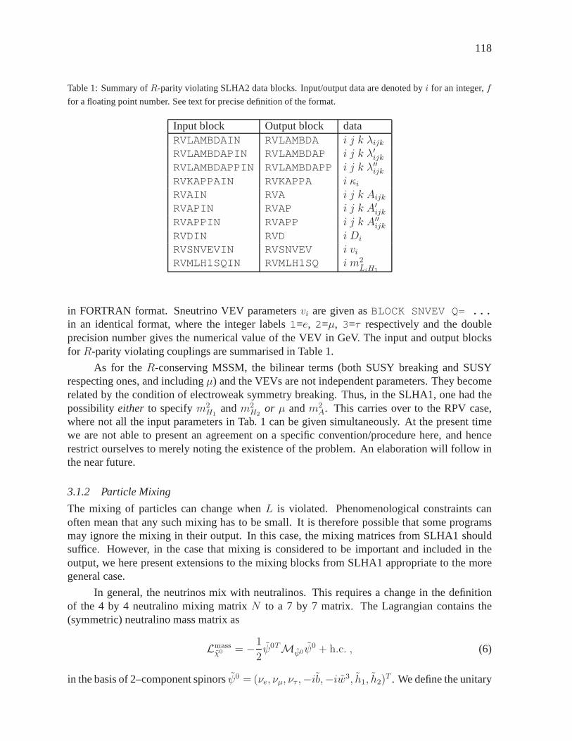
118

Table 1: Summary ofR-parity violating SLHA2 data blocks. Input/output data aredenoted byi for an integer,f

for a floating point number. See text for precise definition ofthe format.

Input block Output block dataRVLAMBDAIN RVLAMBDA i j k λijkRVLAMBDAPIN RVLAMBDAP i j k λ′ijkRVLAMBDAPPIN RVLAMBDAPP i j k λ′′ijkRVKAPPAIN RVKAPPA i κiRVAIN RVA i j k AijkRVAPIN RVAP i j k A′

ijk

RVAPPIN RVAPP i j k A′′ijk

RVDIN RVD i Di

RVSNVEVIN RVSNVEV i viRVMLH1SQIN RVMLH1SQ i m2

LiH1

in FORTRAN format. Sneutrino VEV parametersvi are given asBLOCK SNVEV Q= ...in an identical format, where the integer labels1=e, 2=µ, 3=τ respectively and the doubleprecision number gives the numerical value of the VEV in GeV.The input and output blocksfor R-parity violating couplings are summarised in Table 1.

As for theR-conserving MSSM, the bilinear terms (both SUSY breaking and SUSYrespecting ones, and includingµ) and the VEVs are not independent parameters. They becomerelated by the condition of electroweak symmetry breaking.Thus, in the SLHA1, one had thepossibility either to specifym2

H1andm2

H2or µ andm2

A. This carries over to the RPV case,where not all the input parameters in Tab. 1 can be given simultaneously. At the present timewe are not able to present an agreement on a specific convention/procedure here, and hencerestrict ourselves to merely noting the existence of the problem. An elaboration will follow inthe near future.

3.1.2 Particle Mixing

The mixing of particles can change whenL is violated. Phenomenological constraints canoften mean that any such mixing has to be small. It is therefore possible that some programsmay ignore the mixing in their output. In this case, the mixing matrices from SLHA1 shouldsuffice. However, in the case that mixing is considered to be important and included in theoutput, we here present extensions to the mixing blocks fromSLHA1 appropriate to the moregeneral case.

In general, the neutrinos mix with neutralinos. This requires a change in the definitionof the 4 by 4 neutralino mixing matrixN to a 7 by 7 matrix. The Lagrangian contains the(symmetric) neutralino mass matrix as

Lmassχ0 = −1

2ψ0TMψ0ψ

0 + h.c. , (6)

in the basis of 2–component spinorsψ0 = (νe, νµ, ντ ,−ib,−iw3, h1, h2)T . We define the unitary

119

7 by 7 neutralino mixing matrixN (blockRVNMIX), such that:

−1

2ψ0TMψ0ψ

0 = −1

2ψ0TNT

︸ ︷︷ ︸

χ0T

N∗Mψ0N†

︸ ︷︷ ︸

diag(mχ0 )

Nψ0

︸︷︷︸

χ0

, (7)

where the 7 (2–component) generalised neutralinosχi are defined strictly mass-ordered, i.e.with the 1st,2nd,3rd lightest corresponding to the mass entries for the PDG codes12 , 14 , and16 , and the four heaviest to the PDG codes1000022 , 1000023 , 1000025 , and1000035 .

Note! although these codes are normally associated with names that imply a specificflavour content, such as code12 beingνe and so forth, it would be exceedingly complicated tomaintain such a correspondence in the context of completelygeneral mixing, hence we do notmake any such association here. The flavour content of each state, i.e. of each PDG number,is in general onlydefined by its corresponding entries in the mixing matrixRVNMIX. Note,however, that the flavour basis is ordered so as to reproduce the usual associations in the trivialcase (modulo the unknown flavour composition of the neutrinomass eigenstates).

In the limit of CP conservation, the default convention is thatN be a real symmetric matrixand the neutralinos may have an apparent negative mass. The minus sign may be removed byphase transformations onχ0

i as explained in SLHA1 [92].

Charginos and charged leptons may also mix in the case ofL-violation. In a similar spiritto the neutralino mixing, we define

Lmassχ+ = −1

2ψ−TMψ+ψ

+ + h.c. , (8)

in the basis of 2–component spinorsψ+ = (e′+, µ′+, τ ′+,−iw+, h+2 )T , ψ− = (e′−, µ′−, τ ′−,

−iw−, h−1 )T wherew± = (w1 ∓ w2)/√

2, and the primed fields are in the weak interactionbasis.

We define the unitary 5 by 5 charged fermion mixing matricesU, V , blocksRVUMIX,RVVMIX, such that:

−1

2ψ−TMψ+ψ

+ = −1

2ψ−TUT

︸ ︷︷ ︸

χ−T

U∗Mψ+V†

︸ ︷︷ ︸

diag(mχ+ )

V ψ+

︸︷︷︸

χ+

, (9)

whereχ±i are defined as strictly mass ordered, i.e. with the 3 lighteststates corresponding to the

PDG codes11 , 13 , and15 , and the two heaviest to the codes1000024 , 1000037 . As forneutralino mixing, the flavour content of each state is in no way implied by its PDG number,but is onlydefined by its entries inRVUMIXandRVVMIX. Note, however, that the flavour basisis ordered so as to reproduce the usual associations in the trivial case.

In the limit of CP conservation,U, V are be chosen to be real by default.

CP-even Higgs bosons mix with sneutrinos in the limit of CP symmetry. We write theneutral scalars asφ0

i ≡√

2Re(H0

1 , H02 , νe, νµ, ντ )

T

L = −1

2φ0TM2

φ0φ0 (10)

whereM2φ0 is a 5 by 5 symmetric mass matrix.

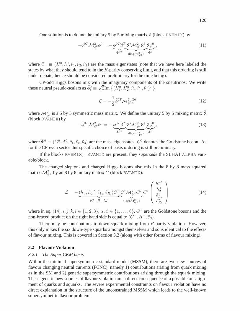
120

One solution is to define the unitary 5 by 5 mixing matrixℵ (block RVHMIX) by

−φ0TM2φ0φ0 = −φ0TℵT

︸ ︷︷ ︸

Φ0T

ℵ∗M2φ0ℵ†

︸ ︷︷ ︸

diag(m2

Φ0)

ℵφ0

︸︷︷︸

Φ0

, (11)

whereΦ0 ≡ (H0, h0, ν1, ν2, ν3) are the mass eigenstates (note that we have here labeled thestates by what they should tend to in theR-parity conserving limit, and that this ordering is stillunder debate, hence should be considered preliminary for the time being).

CP-odd Higgs bosons mix with the imaginary components of thesneutrinos: We writethese neutral pseudo-scalars asφ0

i ≡√

2Im(H0

1 , H02 , νe, νµ, ντ )

T

L = −1

2φ0TM2

φ0φ0 (12)

whereM2φ0 is a 5 by 5 symmetric mass matrix. We define the unitary 5 by 5 mixing matrix ℵ

(blockRVAMIX) by−φ0TM2

φ0φ0 = − φ0T ℵT

︸ ︷︷ ︸

Φ0T

ℵ∗M2φ0ℵ†

︸ ︷︷ ︸

diag(m2

Φ0)

ℵφ0

︸︷︷︸

Φ0

, (13)

whereΦ0 ≡ (G0, A0, ν1, ν2, ν3) are the mass eigenstates.G0 denotes the Goldstone boson. Asfor the CP-even sector this specific choice of basis orderingis still preliminary.

If the blocksRVHMIX, RVAMIXare present, theysupersedethe SLHA1ALPHAvari-able/block.

The charged sleptons and charged Higgs bosons also mix in the8 by 8 mass squaredmatrixM2

φ± by an 8 by 8 unitary matrixC (block RVLMIX):

L = − (h−1 , h+2∗, eLi

, eRj)CT

︸ ︷︷ ︸

(G−,H−,eα)

C∗M2φ±C

T

︸ ︷︷ ︸

diag(M2

Φ± )

C∗

h−1∗

h+2

e∗Lk

e∗Rl

(14)

where in eq. (14),i, j, k, l ∈ 1, 2, 3, α, β ∈ 1, . . . , 6,G± are the Goldstone bosons and thenon-braced product on the right hand side is equal to(G+, H+, eβ).

There may be contributions to down-squark mixing fromR-parity violation. However,this only mixes the six down-type squarks amongst themselves and so is identical to the effectsof flavour mixing. This is covered in Section 3.2 (along with other forms of flavour mixing).

3.2 Flavour Violation

3.2.1 The Super CKM basis

Within the minimal supersymmetric standard model (MSSM), there are two new sources offlavour changing neutral currents (FCNC), namely 1) contributions arising from quark mixingas in the SM and 2) generic supersymmetric contributions arising through the squark mixing.These generic new sources of flavour violation are a direct consequence of a possible misalign-ment of quarks and squarks. The severe experimental constraints on flavour violation have nodirect explanation in the structure of the unconstrained MSSM which leads to the well-knownsupersymmetric flavour problem.

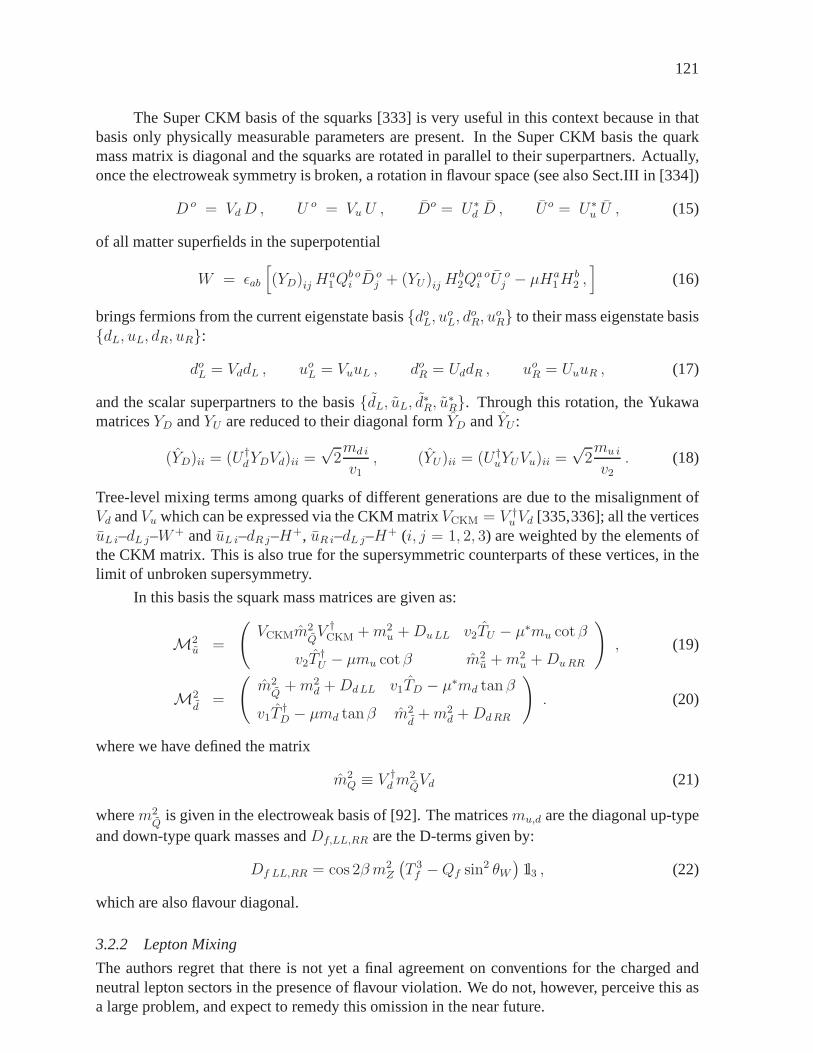
121

The Super CKM basis of the squarks [333] is very useful in thiscontext because in thatbasis only physically measurable parameters are present. In the Super CKM basis the quarkmass matrix is diagonal and the squarks are rotated in parallel to their superpartners. Actually,once the electroweak symmetry is broken, a rotation in flavour space (see also Sect.III in [334])

D o = VdD , U o = Vu U , Do = U∗d D , Uo = U∗

u U , (15)

of all matter superfields in the superpotential

W = ǫab

[

(YD)ij Ha1Q

b oi D

oj + (YU)ij H

b2Q

a oi U

oj − µHa

1Hb2 ,]

(16)

brings fermions from the current eigenstate basisdoL, uoL, doR, uoR to their mass eigenstate basisdL, uL, dR, uR:

doL = VddL , uoL = VuuL , doR = UddR , uoR = UuuR , (17)

and the scalar superpartners to the basisdL, uL, d∗R, u∗R. Through this rotation, the YukawamatricesYD andYU are reduced to their diagonal formYD andYU :

(YD)ii = (U †dYDVd)ii =

√2md i

v1

, (YU)ii = (U †uYUVu)ii =

√2mu i

v2

. (18)

Tree-level mixing terms among quarks of different generations are due to the misalignment ofVd andVu which can be expressed via the CKM matrixVCKM = V †

uVd [335,336]; all the verticesuL i–dL j–W+ anduL i–dRj–H+, uR i–dL j–H+ (i, j = 1, 2, 3) are weighted by the elements ofthe CKM matrix. This is also true for the supersymmetric counterparts of these vertices, in thelimit of unbroken supersymmetry.

In this basis the squark mass matrices are given as:

M2u =

(

VCKMm2QV †

CKM +m2u +DuLL v2TU − µ∗mu cot β

v2T†U − µmu cotβ m2

u +m2u +DuRR

)

, (19)

M2d

=

(

m2Q

+m2d +DdLL v1TD − µ∗md tan β

v1T†D − µmd tanβ m2

d+m2

d +DdRR

)

. (20)

where we have defined the matrix

m2Q ≡ V †

dm2QVd (21)

wherem2Q

is given in the electroweak basis of [92]. The matricesmu,d are the diagonal up-typeand down-type quark masses andDf,LL,RR are the D-terms given by:

Df LL,RR = cos 2β m2Z

(T 3f −Qf sin2 θW

)1l3 , (22)

which are also flavour diagonal.

3.2.2 Lepton Mixing

The authors regret that there is not yet a final agreement on conventions for the charged andneutral lepton sectors in the presence of flavour violation.We do not, however, perceive this asa large problem, and expect to remedy this omission in the near future.

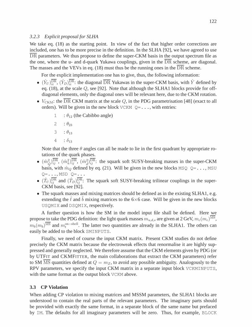
122

3.2.3 Explicit proposal for SLHA

We take eq. (18) as the starting point. In view of the fact thathigher order corrections areincluded, one has to be more precise in the definition. In the SLHA [92], we have agreed to useDR parameters. We thus propose to define the super-CKM basis in the output spectrum file asthe one, where the u- and d-quark Yukawa couplings, given in theDR scheme, are diagonal.The masses and the VEVs in eq. (18) must thus be the running ones in theDR scheme.

For the explicit implementation one has to give, thus, the following information:

• (YU)DRii , (YD)DR

ii : the diagonalDR Yukawas in the super-CKM basis, withY defined byeq. (18), at the scaleQ, see [92]. Note that although the SLHA1 blocks provide for off-diagonal elements, only the diagonal ones will be relevant here, due to the CKM rotation.

• VCKM: theDR CKM matrix at the scaleQ, in the PDG parametrisation [48] (exact to allorders). Will be given in the new blockVCKM Q=... , with entries:

1 : θ12 (the Cabibbo angle)

2 : θ23

3 : θ13

4 : δ13

Note that the threeθ angles can all be made to lie in the first quadrant by appropriate ro-tations of the quark phases.

• (m2Q)DRij , (m2

u)DRij , (m2

d)DRij : the squark soft SUSY-breaking masses in the super-CKM

basis, withmQ defined by eq. (21). Will be given in the new blocksMSQ Q=... , MSUQ=... , MSD Q=...

• (TU)DRij and (TD)DR

ij : The squark soft SUSY-breaking trilinear couplings in the super-CKM basis, see [92].

• The squark masses and mixing matrices should be defined as in the existing SLHA1, e.g.extending thet and b mixing matrices to the 6×6 case. Will be given in the new blocksUSQMIXandDSQMIX, respectively.

A further question is how the SM in the model input file shall bedefined. Here wepropose to take the PDG definition: the light quark massesmu,d,s are given at 2 GeV,mc(mc)

MS,mb(mb)

MS andmon−shellt . The latter two quantities are already in the SLHA1. The others can

easily be added to the blockSMINPUTS.

Finally, we need of course the input CKM matrix. Present CKM studies do not defineprecisely the CKM matrix because the electroweak effects that renormalise it are highly sup-pressed and generally neglected. We therefore assume that the CKM elements given by PDG (orby UTFIT and CKMFITTER, the main collaborations that extract the CKM parameters) referto SM MS quantities defined atQ = mZ , to avoid any possible ambiguity. Analogously to theRPV parameters, we specify the input CKM matrix in a separateinput blockVCKMINPUTS,with the same format as the output blockVCKMabove.

3.3 CP Violation

When adding CP violation to mixing matrices and MSSM parameters, the SLHA1 blocks areunderstood to contain the real parts of the relevant parameters. The imaginary parts shouldbe provided with exactly the same format, in a separate blockof the same name but prefacedby IM . The defaults for all imaginary parameters will be zero. Thus, for example,BLOCK

123

IMAU, IMAD, IMAE, Q= ... would describe the imaginary parts of the trilinear softSUSY-breaking scalar couplings. For input,BLOCK IMEXTPARmay be used to provide therelevant imaginary parts of soft SUSY-breaking inputs. In cases where the definitions of thecurrent paper supersedes the SLHA1 input and output blocks,completely equivalent statementsapply.

The Higgs sector mixing changes when CP symmetry is broken, since the CP-even andCP-odd Higgs states mix. Writing the neutral scalars asφ0

i ≡√

2(Re H01 ,Re H0

2 , Im H01 ,

Im H02) we define the unitary 4 by 4 mixing matrixS (blocksCVHMIXandIMCVHMIX) by

−φ0TM2φ0φ0 = −φ0TST

︸ ︷︷ ︸

Φ0T

S∗M2φ0S†

︸ ︷︷ ︸

diag(m2

Φ0)

Sφ0

︸︷︷︸

Φ0

, (23)

whereΦ0 ≡ (G0, H01 , H

02 , H

03 ) are the mass eigenstates.G0 denotes the Goldstone boson. We

associate the following PDG codes with these states, in strict mass orderregardlessof CP-even/odd composition:H0

1 : 25,H02 : 35,H0

3 : 36. That is, even though the PDG reserves code36 for the CP-odd state, we do not maintain such a labeling here, nor one that reduces to it. Thismeans one does have to exercise some caution when taking the CP conserving limit.

Whether and how to include the mixing in the charged Higgs sector (specifying the make-up of (G+, H+) in terms of their(H+

1 , H+2 ) components) has not yet been agreed upon.

4. THE NEXT-TO-MINIMAL SUPERSYMMETRIC STANDARD MODEL

4.1 Conventions

In the notation of SLHA1 the conventions for the Lagrangian of the CP conserving NMSSMare as follows: The NMSSM specific terms in the superpotential W are given by

W = −ǫabλSHa1H

b2 +

1

3κS3 . (24)

Hence a VEV〈S〉 of the singlet generates an effectiveµ termµeff = λ 〈S〉. (Note that the signof theλ term in eq. (24) coincides with the one in [218,305] where theHiggs doublet superfieldsappear in opposite order.) The new soft SUSY-breaking termsare

Vsoft = m2S|S|2 + (−ǫabλAλSHa

1Hb2 +

1

3κAκS

3 + h.c.) . (25)

The input parameters relevant for the Higgs sector of the NMSSM (at tree level) are

λ, κ, Aλ, Aκ, tanβ = 〈H2〉 / 〈H1〉 , µeff = λ 〈S〉 . (26)

One can choose sign conventions such thatλ andtan β are positive, whileκ, Aλ, Aκ andµeff

must be allowed to have either sign.

4.2 Input/Output Blocks

TheBLOCK MODSELshould contain the switch 3 (corresponding to the choice of the model)with value 1, as attributed to the NMSSM already in SLHA1. TheBLOCK EXTPARcontainsthe NMSSM specific SUSY and soft SUSY-breaking parameters. The new entries are:

124

61 forλ62 forκ63 forAλ64 forAκ65 forµeff = λ 〈S〉

Note that the meaning of the switch 23 (the MSSMµ parameter) is maintained which allows,in principle, for non zero values for bothµ andµeff . The reason for choosingµeff rather than〈S〉 as input parameter 65 is that it allows more easily to recoverthe MSSM limitλ, κ → 0,〈S〉 → ∞ with λ 〈S〉 fixed.

Proposed PDG codes for the new states in the NMSSM (to be used in theBLOCK MASSand the decay files, see also Section 5.) are

45 for the third CP-even Higgs boson,46 for the second CP-odd Higgs boson,1000045 for the fifth neutralino.

4.3 Particle Mixing

In the CP-conserving NMSSM, the diagonalisation of the3 × 3 mass matrix in the CP-evenHiggs sector can be performed by an orthogonal matrixSij . The (neutral) CP-even Higgs weakeigenstates are numbered byφ0

i ≡√

2Re(H0

1 , H02 , S)T

. If Φi are the mass eigenstates

(ordered in mass), the convention isΦi = Sijφ0j . The elements ofSij should be given in a

BLOCK NMHMIX, in the same format as the mixing matrices in SLHA1.

In the MSSM limit (λ, κ → 0, and parameters such thath3 ∼ SR) the elements of thefirst 2 × 2 sub-matrix ofSij are related to the MSSM angleα as

S11 ∼ cosα , S21 ∼ sinα ,

S12 ∼ − sinα , S22 ∼ cosα .

In the CP-odd sector the weak eigenstates areφ0i ≡

√2Im

(H0

1 , H02 , S)T

. We define

the orthogonal 3 by 3 mixing matrixP (blockNMAMIX) by

−φ0TM2φ0φ

0 = − φ0TP T

︸ ︷︷ ︸

Φ0T

PM2φ0P

T

︸ ︷︷ ︸

diag(m2

Φ0)

P φ0

︸︷︷︸

Φ0

, (27)

whereΦ0 ≡ (G0, A01, A

02) are the mass eigenstates ordered in mass.G0 denotes the Goldstone

boson. Hence,Φi = Pijφ0j . (Note that some of thePij are redundant sinceP11 = cosβ,

P12 = − sin β,P13 = 0, and the present convention does not quite coincide with theone in [218]where redundant information has been omitted. An updated version of [305] will include theSLHA2 conventions.)

If NMHMIX, NMAMIXblocks are present, theysupersedethe SLHA1ALPHAvariable/block.

The neutralino sector of the NMSSM requires a change in the definition of the 4 by 4neutralino mixing matrixN to a 5 by 5 matrix. The Lagrangian contains the (symmetric)neutralino mass matrix as

Lmassχ0 = −1

2ψ0TMψ0ψ

0 + h.c. , (28)

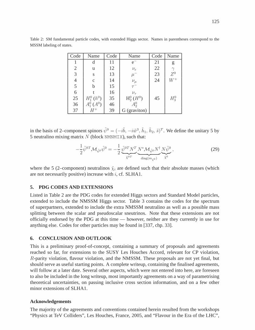
125

Table 2: SM fundamental particle codes, with extended Higgssector. Names in parentheses correspond to the

MSSM labeling of states.

Code Name Code Name Code Name1 d 11 e− 21 g2 u 12 νe 22 γ3 s 13 µ− 23 Z0

4 c 14 νµ 24 W+

5 b 15 τ−

6 t 16 ντ25 H0

1 (h0) 35 H02 (H0) 45 H0

3

36 A01 (A0) 46 A0

2

37 H+ 39 G (graviton)

in the basis of 2–component spinorsψ0 = (−ib, −iw3, h1, h2, s)T . We define the unitary 5 by

5 neutralino mixing matrixN (block NMNMIX), such that:

−1

2ψ0TMψ0ψ

0 = −1

2ψ0TNT

︸ ︷︷ ︸

χ0T

N∗Mψ0N†

︸ ︷︷ ︸

diag(mχ0 )

Nψ0

︸︷︷︸

χ0

, (29)

where the 5 (2–component) neutralinosχi are defined such that their absolute masses (whichare not necessarily positive) increase withi, cf. SLHA1.

5. PDG CODES AND EXTENSIONS

Listed in Table 2 are the PDG codes for extended Higgs sectorsand Standard Model particles,extended to include the NMSSM Higgs sector. Table 3 containsthe codes for the spectrumof superpartners, extended to include the extra NMSSM neutralino as well as a possible masssplitting between the scalar and pseudoscalar sneutrinos.Note that these extensions are notofficially endorsed by the PDG at this time — however, neitherare they currently in use foranything else. Codes for other particles may be found in [337, chp. 33].

6. CONCLUSION AND OUTLOOK

This is a preliminary proof-of-concept, containing a summary of proposals and agreementsreached so far, for extensions to the SUSY Les Houches Accord, relevant for CP violation,R-parity violation, flavour violation, and the NMSSM. These proposals are not yet final, butshould serve as useful starting points. A complete writeup,containing the finalised agreements,will follow at a later date. Several other aspects, which were not entered into here, are foreseento also be included in the long writeup, most importantly agreements on a way of parametrisingtheoretical uncertainties, on passing inclusive cross section information, and on a few otherminor extensions of SLHA1.

Acknowledgements

The majority of the agreements and conventions contained herein resulted from the workshops“Physics at TeV Colliders”, Les Houches, France, 2005, and “Flavour in the Era of the LHC”,

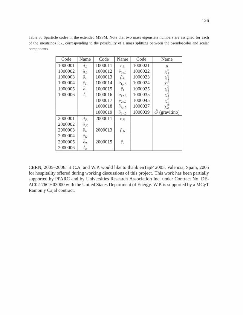
126

Table 3: Sparticle codes in the extended MSSM. Note that two mass eigenstate numbers are assigned for each

of the sneutrinosνiL, corresponding to the possibility of a mass splitting between the pseudoscalar and scalar

components.

Code Name Code Name Code Name1000001 dL 1000011 eL 1000021 g1000002 uL 1000012 ν1eL 1000022 χ0

1

1000003 sL 1000013 µL 1000023 χ02

1000004 cL 1000014 ν1µL 1000024 χ±1

1000005 b1 1000015 τ1 1000025 χ03

1000006 t1 1000016 ν1τL 1000035 χ04

1000017 ν2eL 1000045 χ05

1000018 ν2µL 1000037 χ±2

1000019 ν2τL 1000039 G (gravitino)2000001 dR 2000011 eR2000002 uR2000003 sR 2000013 µR2000004 cR2000005 b2 2000015 τ22000006 t2

CERN, 2005–2006. B.C.A. and W.P. would like to thank enTapP 2005, Valencia, Spain, 2005for hospitality offered during working discussions of thisproject. This work has been partiallysupported by PPARC and by Universities Research Association Inc. under Contract No. DE-AC02-76CH03000 with the United States Department of Energy. W.P. is supported by a MCyTRamon y Cajal contract.

127

Part 17

Pythia UED : a Pythia-based generatortool for universal extra dimensions at theLHCM. ElKacimi, D. Goujdami and H. Przysiezniak

AbstractTheories with extra dimensions offer a description of the gravitationalinteraction at low energy, and thus receive considerable attention. Onevery interesting incarnation was formulated by Appelquist, Cheng andDobrescu [314], the Universal Extra Dimensions (UED) model, whereUniversalcomes from the fact that all Standard Model (SM) fields prop-agate into the extra dimensions.

We provide a Pythia-based [17] generator tool which will enable us tostudy the UED model with one extra dimension and additional gravitymediated decays [315], using in particular the ATLAS detector at theLHC.

1. INTRODUCTION

Extra dimensions accessible to Standard Model fields are of interest for various reasons. Theycould allow gauge coupling unification [338], and provide new mechanisms for supersymmetrybreaking [339] and the generation of fermion mass hierarchies [340]. It has also been shownthat extra dimensions accessible to the observed fields may lead to the existence of a Higgsdoublet [341].

In the UED model, the SM lives in4 + δ space-time dimensions. This effective theory isvalid below some scaleΛ (cutoff scale). The compactification scale is1/R < Λ for theδ extraspatial dimensions. To avoid fine-tuning the parameters in the Higgs sector,1/R should not bemuch higher than the electroweak scale.

Lower bounds can be set on1/R from precision electroweak observables [342–345]. Inthe case of a single extra dimension (δ = 1), using the upper bound on isospin breaking effects,Appelquist etal. [314] find:1/R ≥ 300 GeV. As well, the loop expansion parameterǫ3 becomesof order unity, indicating breakdown of the effective theory, at roughly 10 TeV. The presentlimit from direct non-detection is1/R ≥ 300 GeV, for one extra dimension [314]. Appelquistetal. also show that for more than one extra dimension (δ ≥ 2), the T (isospin breaking) andS (electroweak gauge bosons mixing) parameters and other electroweak observables becomecutoff dependent. Forδ = 2, the lower bound on1/R is approximately 400 to 800 GeV, forΛR = 2 to 5. Forδ ≥ 3, the cutoff dependence is more severe and no reliable estimate ispossible in this case.

The UED phenomenology shows interesting parallels to supersymmetry. Every SM fieldhas Kaluza Klein (KK) partners. The lowest level KK excitations carry a conserved quantumnumber, KK parity, which guarantees that the lightest KK particle (LKP) is stable. Heavier KK

128

modes cascade decay to the LKP by emitting soft SM particles.The LKP escapes detection,resulting in missing energy signals, unless some other mechanism enables it to decay.

2. THE UED MODEL DESCRIPTION

2.1 Momentum and KK number conservation

One can consider the case of a massless field propagating in a single, compactified, circularextra dimension of radius R (TeV−1 sized). This theory is equivalently described by a fourdimensional theory with a tower of states (KK excitations) with tree level massesmn = n/R.The integern corresponds to the quantized momentump5 in the compact dimension and be-comes a quantum number (KK number) under aU(1) symmetry in the 4D description. The treelevel dispersion relation of a 5D massless particle is fixed by Lorentz invariance of the tree levelLagrangianE2 = ~p2 + p2

5 = ~p2 + m2n, where~p is the momentum in the usual three spatial

directions. Ignoring branes and orbifold fixed points, KK number is a good quantum numberand is preserved in all interactions and decays. It is also straightforward to include electroweaksymmetry breaking masses, such that the KK mass relation is given by :

mKKn = (m2

n +m2SM)1/2 = (n2/R2 +m2

SM)1/2 (1)

wheremSM stands for the SM particle mass.

The key element of this model is the conservation of momentumin the extra dimensions,which becomes, after compactification, conservation of theKK number (also called KK mo-mentum) in the equivalent 4D theory. There may be some boundary terms that break the KKnumber conservation (see Section 3.1), but the KK parity is preserved. There are hence novertices involving only one non-zero KK mode, and non-zero KK modes may be produced atcolliders only in groups of two or more.

2.2 The Lagrangian

The notationxα, α = 0, 1, ..., 3 + δ is used for the coordinates of the4 + δ dimensional space-time, whilexµ, µ = 0, 1, 2, 3 andya, a = 1, ..., δ correspond respectively to the usual non-compact space-time coordinates and to the extra dimensionscoordinates. From Appelquistetal. [314], the4 + δ dimensional Lagrangian is given by:

L(xµ) =

∫

dδy

−3∑

i=1

1

2g2i

Tr[F αβi (xµ, ya)Fi αβ(x

µ, ya)]+ LHiggs(x

µ, ya)

+ i(Q, U , D

)(xµ, ya)

(ΓµDµ + Γ3+aD3+a

)(Q,U ,D

)†(xµ, ya)

+[Q(xµ, ya)

(λUU(xµ, ya)iσ2H

∗(xµ, ya) + λDD(xµ, ya)H(xµ, ya))

+h.c.]

(2)

whereF αβi are the4 + δ dimensional gauge field strenghts associated with theSU(3)C ×

SU(2)W × U(1)Y group, whileDµ = ∂/∂xµ − Aµ andD3+a = ∂/∂ya − A3+a are the co-variant derivatives withAα = −i

∑3i=1 giAr

αiTri being the4 + δ dimensional gauge fields.

LHiggs contains the kinetic term for the4 + δ dimensional Higgs doublet H, and the Higgs po-tential. The fieldsQ (doublet),U andD (singlets) correspond to the4 + δ dimensional quarks,for which the zero modes are given by the SM quarks.

129

In order to derive the 4D Lagrangian, the compactification ofthe extra dimensions hasto be specified. Forδ = 1, the UED choice [314] is anS1/Z2 orbifold. A description ofthe compactification is given by a one-dimensional space with coordinate0 ≤ y ≤ πR, andboundary conditions such that each field or its derivative with respect toy vanish at the orbifoldfixed pointsy = 0,±πR.

The Lagrangian together with the boundary conditions completely specifies the theory.The momentum conservation in the extra dimensions, implicitly associated with the Lagrangianabove, is preserved by the orbifold projection. However, obtaining chiral fermions in 4 dimen-sions from a 5D (δ = 1) theory is only possible with additional breaking of 5D Lorentz invari-ance. This is done by imposing orbifold boundary conditionson fermions in the bulk. This willbe described in Section 3.1.

2.3 KK particle spectrum for one extra dimension

For one extra dimension (δ = 1), at each KK level (n = 1, 2, ...) one will find a set of fieldsincluding theSU(3)C ×SU(2)W ×U(1)Y gauge fields, three generations of vector-like quarksand leptons, a Higgs doublet, andδ = 1 scalar in the adjoint representations of the gauge. Inthe SM, the quark multiplets for theith generation are :

QSMi (x) =

(

ui(x)di(x)

)

L

, USMi (x) = uRi (x), DSM

i (x) = dRi (x).

In 4 + 1 dimensions, theith generation fermion doubletsQi (quarks) andLi (leptons), andsingletsUi,Di (quarks) andEi (lepton) are four-component and contain both chiralities (left andright) when reduced to3 + 1 dimensions. Under theS1/Z2 orbifold symmetry,QL, UR, DR,LL, ER are even such that they have zero modes associated with the SMfermions. The fermionswith opposite chirality,QR, UL, DL, LR, EL are odd, and their zero modes are projected out.The mass eigenstatesU ′n

i andQ′ni have the same mass(m2

n +m2i )

1/2.

The weak eigenstate neutral gauge bosons mix level by level in the same way as the neutralSU(2)W and hypercharge gauge bosons in the SM. The corresponding mass eigenstates,Z i

µ andAiµ have masses(m2

n +m2Z)1/2 andmn respectively. The heavy gauge bosons have interactions

with one zero-mode quark and one n-mode quark, identical to the SM interactions of the zero-modes.

Each non-zero KK mode of the Higgs doubletHn includes a charged Higgs and a neutralCP-odd scalar of massmn, and also a neutral CP even scalar of mass(m2

n + m2H)1/2. The

interactions of the KK Higgs and gauge bosons may also be obtained from the correspondingSM interactions of the zero-modes by replacing two of the fields at each vertex with theirnthKK mode.

The mass spectrum at each KK level is highly degenerate except for particles with largezero mode masses (t, W, Z, h).

3. KK DECAYS AND THE MINIMAL UED MODEL

If the KK number conservation is exact, some of the KK excitations of the SM particles willbe stable. Such heavy stable charged particles will cause cosmological problems if a significantnumber of them survive at the time of nucleosynthesis [346, 347]. They would combine withother nuclei to form heavy hydrogen atoms. Searches for suchheavy isotopes put strong limits

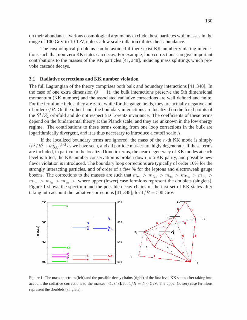
130

on their abundance. Various cosmological arguments exclude these particles with masses in therange of 100 GeV to 10 TeV, unless a low scale inflation dilutestheir abundance.

The cosmological problems can be avoided if there exist KK-number violating interac-tions such that non-zero KK states can decay. For example, loop corrections can give importantcontributions to the masses of the KK particles [41, 348], inducing mass splittings which pro-voke cascade decays.

3.1 Radiative corrections and KK number violation

The full Lagrangian of the theory comprises both bulk and boundary interactions [41, 348]. Inthe case of one extra dimension (δ = 1), the bulk interactions preserve the 5th dimensionalmomentum (KK number) and the associated radiative corrections are well defined and finite.For the fermionic fields, they are zero, while for the gauge fields, they are actually negative andof orderα/R. On the other hand, the boundary interactions are localizedon the fixed points oftheS1/Z2 orbifold and do not respect 5D Lorentz invariance. The coefficients of these termsdepend on the fundamental theory at the Planck scale, and they are unknown in the low energyregime. The contributions to these terms coming from one loop corrections in the bulk arelogarithmically divergent, and it is thus necessary to introduce a cutoff scaleΛ.

If the localized boundary terms are ignored, the mass of then-th KK mode is simply(n2/R2 +m2

SM )1/2 as we have seen, and all particle masses are higly degenerate. If these termsare included, in particular the localized kinetic terms, the near-degeneracy of KK modes at eachlevel is lifted, the KK number conservation is broken down toa KK parity, and possible newflavor violation is introduced. The boundary loop corrections are typically of order 10% for thestrongly interacting particles, and of order of a few % for the leptons and electroweak gaugebosons. The corrections to the masses are such thatmgn > mQn > mqn > mWn > mZn >mLn > mℓn > mγn >, where upper (lower) case fermions represent the doublets (singlets).Figure 1 shows the spectrum and the possible decay chains of the first set of KK states aftertaking into account the radiative corrections [41,348], for 1/R = 500 GeV.

Figure 1: The mass spectrum (left) and the possible decay chains (right) of the first level KK states after taking into

account the radiative corrections to the masses [41, 348], for 1/R = 500 GeV. The upper (lower) case fermions

represent the doublets (singlets).

131

3.2 Minimal UED scenario

The minimal UED scenario has only one extra dimension (δ = 1). The assumption is madethat all boundary terms are negligible at some scaleΛ > R−1. This is completely analogousto the case of the Minimal SUSY SM (MSSM) where one has to choose a set of soft SUSYbreaking couplings at some high scale before studying the phenomenology. The choice ofboundary couplings may be viewed as analogous to the simplest minimal SUGRA boundarycondition: universal scalar and gaugino masses. The minimal UED (MUED) model is extremelypredictive, and has only three free parameters:

R,Λ, mH

wheremH is the mass of the SM Higgs boson.

The lightest KK particle (LKP)γ1 (n=1 KK state of the SM photon) is a mixture of thefirst KK modeB1 of theU(1)Y gauge bosonB and the first KK modeW 0

1 of theSU(2)W W 3

gauge boson. The correspondingWeinbergangleθ1 is much smaller thanθW of the SM, so thattheγ1 is mostlyB1 andZ1 is mostlyW 0

1 . The spectrum is still quite degenerate, such that theSM particles emitted from these mass splitting decays will be soft. Each level 1 KK particle hasan exact analogue in SUSY:B1 ↔ bino, g1 ↔ gluino,Q1(q1) ↔ left-handed (right-handed)squark, etc. The cascade decays of the level 1 KK modes will terminate in the LKP. Just likethe neutralino LSP is stable inR-parity conserving SUSY, the LKP in MUEDs is stable due toKK parity conservation.

The branching ratios for the different level 1 KK particles are given below, where upper(lower) case fermions represent the doublets (singlets):

B(g1 → Q1Q0) ≃ B(g1 → q1q0) ≃ 0.5

B(q1 → Z1q0) ≃ sin2 θ1 ≃ 10−2 − 10−3

B(q1 → γ1q0) ≃ cos2 θ1 ≃ 1

B(Q1 → W±1 Q′

0) ≃ 0.65

B(Q1 → Z1Q0) ≃ 0.33

B(Q1 → γ1Q0) ≃ 0.02

B(W±1 → ν1L

±0 ) = B(W±

1 → L±1 ν0) ≃ 1/6 (for each generation)

B(Z1 → ν1ν0) = B(Z1 → L±1 L∓

0 ) ≃ 1/6 (for each generation)

B(L±1 → γ1L

±0 ) = 1

B(ν1 → γ1ν0) = 1

If they are heavy enough and the phase space is open, the KK Higgs bosons can decay into theKK W and Z bosons or into the KK top and bottom quarks. If they are lighter, their tree-level2-body decays will be suppressed and they will decay asH1 → γ1H0, or H1 → γ1γ through aloop.

4. GRAVITY MEDIATED DECAYS

We have seen that radiative corrections lift the KK mass degeneracy, and thus induce cascadedecays. In addition, some mechanisms can provide for KK decays through gravity mediatedinteractions [315]. In the latter, the level 1 KK particle decays into its SM equivalent plus aKK graviton. It is interesting to study the phenomenology ofa model where both mechanisms

132

occur. If the mass splitting widths of the first level KK excitations are much larger than thegravity mediated widths, the quark and gluon KK excitationscascade down to the LKP (γ1),which then produces a photon plus a KK graviton. The experimental signal is a striking twophoton plus missing energy event.

In the MUED context, the 4+1 dimensional space in which the SMfields propagate maybe a thick brane embedded in a space of NeV−1 sized dimensions where only gravitons prop-agate [315]. The KK excitations can then decay into SM particles plus gravitons going out ofthe thick brane, and the unbalanced momentum in the extra dimensions can be absorbed bythis brane. The lifetime depends on the stength of the coupling to the graviton going out of thebrane and the density of its KK modes. Using the decay widths from Macesanu, McMullenand Nandi [349, 350], as well as the KK mass spectrum of the graviton from Beauchemin andAzuelos [351,352], these type of decays are also consideredin the following analysis.

5. Pythia-BASED GENERATOR TOOL

The aim of the work started during theLes Houches 2005 Workshopwas to implement theMinimal UED scenario with gravity mediated decays in a generator for future use in the contextof the LHC. Some results are shown here for proton-proton collisions at a centre-of-mass energyof 14 TeV. The MUED model, where all SM fields propagate into one (δ = 1) TeV−1 sizedextra dimension, embedded in a space of N eV−1 sized dimensions (where only the gravitonpropagates), is implemented in the generator tool described below. Hence, mass splitting decaysas well as gravity mediated decays are possible.

5.1 Production processes, cross sections and decays

To begin with, the CompHep code [353] with UED implementation [44, 354] was used, wherethe pair production of KK particles at the LHC is properly described. The generated events(four-vectors of the hard process) were fed into a modified Pythia, where already existing Pythiaprocesses and particles were replaced by those of the KK particle spectrum.

The model was then implemented inside Pythia, as separate new particles as well asnew production and decay processes. Table 1 lists the production processes found insidePythiaUED, whereg1 andQ1 (q1) are respectively the first level KK gluon and quark dou-blet (singlet). The matrix elements of these processes are implemented, as are the masses andwidths of the particles, including the one-loop radiative corrections [349,350].

The cross-sections versusMKK = 1/R are shown in Figure 2 and are in very goodagreement with those of Beauchemin and Azuelos [351].

The mass splitting and gravity mediated decay widths from [41, 348, 355] which are im-plemented in PythiaUED are shown in Figure 3.

5.2 User advice

From thehttp://wwwlapp.in2p3.fr/ ∼przys/PythiaUED.html web page, thepythia ued med.tar.gzfile can be found, and must be unzipped (i.e.gunzip *.tar.gz) and then untarred (i.e.tar -cvf*.tar ). In the main directory, one finds the main routinepkkprod.f , themakefile, and a scriptcomp execwhich compiles or executespkkprod.f . All other original or modified Pythia rou-tines are in the directorypythia62ued rep. In the job batchdirectory, a script enables to startKK production jobs.

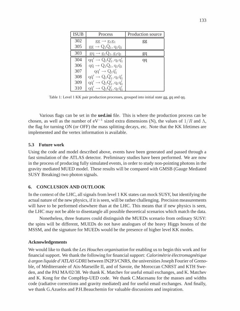
133

ISUB Process Production source

302 gg → g1g1 gg305 gg → Q1Q1, q1q1

303 gq → g1Q1, g1q1 gq

304 qq′ → Q1Q′1, q1q

′1 qq

306 qq → Q1Q1, q1q1

307 qq′ → Q1q′1

308 qq′ → Q1Q′1, q1q

′1

309 qq′ → Q1Q′1, q1q

′1

310 qq′ → Q1Q′1, q1q

′1

Table 1: Level 1 KK pair production processes, grouped into initial state gg, gq and qq.

Various flags can be set in theued.ini file. This is where the production process can bechosen, as well as the number of eV−1 sized extra dimensions (N), the values of1/R andΛ,the flag for turning ON (or OFF) the mass splitting decays, etc. Note that the KK lifetimes areimplemented and the vertex information is available.

5.3 Future work

Using the code and model described above, events have been generated and passed through afast simulation of the ATLAS detector. Preliminary studieshave been performed. We are nowin the process of producing fully simulated events, in orderto study non-pointing photons in thegravity mediated MUED model. These results will be comparedwith GMSB (Gauge MediatedSUSY Breaking) two photon signals.

6. CONCLUSION AND OUTLOOK

In the context of the LHC, all signals from level 1 KK states can mock SUSY, but identifying theactual nature of the new physics, if it is seen, will be ratherchallenging. Precision measurementswill have to be performed elsewhere than at the LHC. This means that if new physics is seen,the LHC may not be able to disentangle all possible theoretical scenarios which match the data.

Nonetheless, three features could distinguish the MUEDs scenario from ordinary SUSY:the spins will be different, MUEDs do not have analogues of the heavy Higgs bosons of theMSSM, and the signature for MUEDs would be the presence of higher level KK modes.

Acknowledgements

We would like to thank theLes Houches organisationfor enabling us to begin this work and forfinancial support. We thank the following for financial support: Calorimetrieelectromagnetiquea argon liquide d’ATLASGDRI between IN2P3/CNRS, the universities Joseph Fourier of Greno-ble, of Mediterranee of Aix-Marseille II, and of Savoie, the Moroccan CNRST and KTH Swe-den, and the PAI MA/02/38. We thank K. Matchev for useful email exchanges, and K. Matchevand K. Kong for the CompHep-UED code. We thank C.Macesanu forthe masses and widthscode (radiative corrections and gravity mediated) and for useful email exchanges. And finally,we thank G.Azuelos and P.H.Beauchemin for valuable discussions and inspiration.

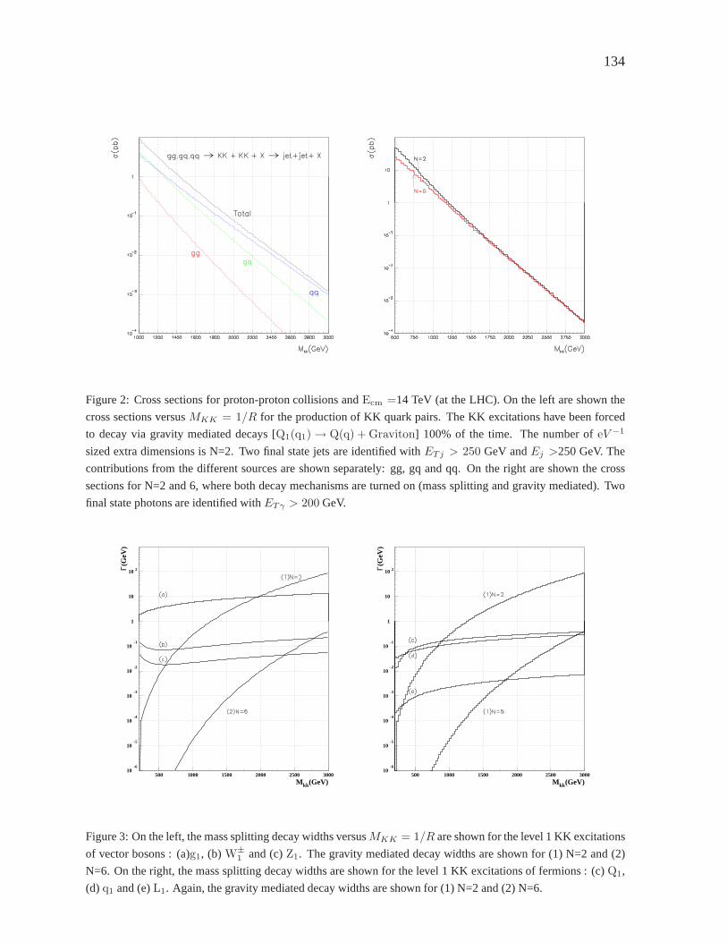
134

Figure 2: Cross sections for proton-proton collisions andEcm =14 TeV (at the LHC). On the left are shown the

cross sections versusMKK = 1/R for the production of KK quark pairs. The KK excitations havebeen forced

to decay via gravity mediated decays [Q1(q1) → Q(q) + Graviton] 100% of the time. The number ofeV −1

sized extra dimensions is N=2. Two final state jets are identified withETj > 250 GeV andEj >250 GeV. The

contributions from the different sources are shown separately: gg, gq and qq. On the right are shown the cross

sections for N=2 and 6, where both decay mechanisms are turned on (mass splitting and gravity mediated). Two

final state photons are identified withETγ > 200 GeV.

10-6

10-5

10-4

10-3

10-2

10-1

1

10

10 2

500 1000 1500 2000 2500 3000

M kk(GeV)

Γ(G

eV)

10-6

10-5

10-4

10-3

10-2

10-1

1

10

10 2

500 1000 1500 2000 2500 3000

M kk(GeV)

Γ(G

eV)

Figure 3: On the left, the mass splitting decay widths versusMKK = 1/R are shown for the level 1 KK excitations

of vector bosons : (a)g1, (b) W±

1 and (c)Z1. The gravity mediated decay widths are shown for (1) N=2 and (2)

N=6. On the right, the mass splitting decay widths are shown for the level 1 KK excitations of fermions : (c)Q1,

(d) q1 and (e)L1. Again, the gravity mediated decay widths are shown for (1) N=2 and (2) N=6.

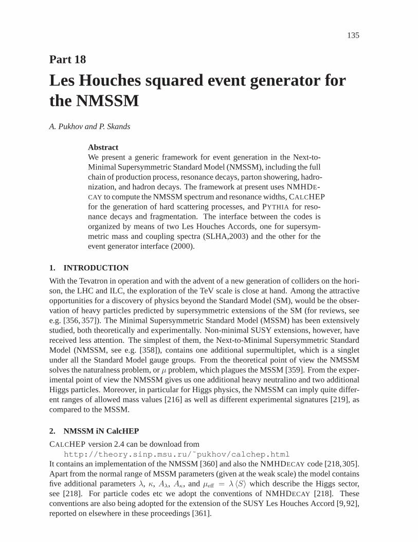
135

Part 18

Les Houches squared event generator forthe NMSSMA. Pukhov and P. Skands

AbstractWe present a generic framework for event generation in the Next-to-Minimal Supersymmetric Standard Model (NMSSM), includingthe fullchain of production process, resonance decays, parton showering, hadro-nization, and hadron decays. The framework at present uses NMHDE-CAY to compute the NMSSM spectrum and resonance widths, CALCHEPfor the generation of hard scattering processes, and PYTHIA for reso-nance decays and fragmentation. The interface between the codes isorganized by means of two Les Houches Accords, one for supersym-metric mass and coupling spectra (SLHA,2003) and the other for theevent generator interface (2000).

1. INTRODUCTION

With the Tevatron in operation and with the advent of a new generation of colliders on the hori-son, the LHC and ILC, the exploration of the TeV scale is closeat hand. Among the attractiveopportunities for a discovery of physics beyond the Standard Model (SM), would be the obser-vation of heavy particles predicted by supersymmetric extensions of the SM (for reviews, seee.g. [356, 357]). The Minimal Supersymmetric Standard Model (MSSM) has been extensivelystudied, both theoretically and experimentally. Non-minimal SUSY extensions, however, havereceived less attention. The simplest of them, the Next-to-Minimal Supersymmetric StandardModel (NMSSM, see e.g. [358]), contains one additional supermultiplet, which is a singletunder all the Standard Model gauge groups. From the theoretical point of view the NMSSMsolves the naturalness problem, orµ problem, which plagues the MSSM [359]. From the exper-imental point of view the NMSSM gives us one additional heavyneutralino and two additionalHiggs particles. Moreover, in particular for Higgs physics, the NMSSM can imply quite differ-ent ranges of allowed mass values [216] as well as different experimental signatures [219], ascompared to the MSSM.

2. NMSSM iN CalcHEP

CALCHEP version 2.4 can be download fromhttp://theory.sinp.msu.ru/˜pukhov/calchep.html

It contains an implementation of the NMSSM [360] and also theNMHDECAY code [218,305].Apart from the normal range of MSSM parameters (given at the weak scale) the model containsfive additional parametersλ, κ, Aλ, Aκ, andµeff = λ 〈S〉 which describe the Higgs sector,see [218]. For particle codes etc we adopt the conventions ofNMHDECAY [218]. Theseconventions are also being adopted for the extension of the SUSY Les Houches Accord [9,92],reported on elsewhere in these proceedings [361].

136

CALCHEP [96] is an interactive menu driven program. It allows theuser to specifyprocesses, generate and compile the corresponding matrix elements, and to launch the obtainedexecutable. In the given case, CALCHEP launches thenmhdecay_slha code which readsthe SLHA input parameter fileslhainp.dat , preliminarily prepared by CALCHEP, thencalculates the spectrum and writes the SLHA output to a file,spectr.dat . The originalSLHA input and output conventions [92] have in this case beensuitably extended to include theNMSSM, see [218,305,361].

Finally, the program allows to check the spectrum against a large variety of experi-mental constraints, using NMHDECAY. Any constraints that are not satisfied are listed inBLOCK SPINFOin the outputspectr.dat file mentioned above. The CALCHEP variableNMHokalso displays the number of broken constraints.

3. THE EVENT GENERATION FRAMEWORK

3.1 Hard Scattering

Partonic2 → N events can be generated by CalcHEP using its menu system, andcan bestored in a file, by default calledevents_N.txt . This file contains information about totalcross section, Monte Carlo numbers of particles involved, initial energies of beams, partonicdistribution functions, and color flows for each event. The first step is thus to generate sucha file, containing a number of partonic events for subsequentfurther processing by a partonshower and hadronisation generator, in our case PYTHIA [17, 46]. For the interface, we makeuse of the Les Houches generator accord [362] — see below for details on the implementation.

3.2 Resonance Decays

If the partonic final state passed to PYTHIA contains heavy unstable particles, a (series of)resonance decay(s) should then follow. However, since PYTHIA does not internally contain anyof the matrix elements relevant to decays involving the new NMSSM states, these partial widthsmust also first be calculated by some other program, and then be passed to PYTHIA togetherwith the event file. For this purpose, we use the SUSY Les Houches Accord [9,92,361], whichincludes a possibility to specify decay tables, whereby information on the total width and decaychannels of any given particle can be transferred between codes.

Both CALCHEP and NMHDECAY can be used to generate such decay tables. ForNMHDECAY, this file decay.dat is generated automatically, but at present it is limited tothe widths and branchings for the Higgs sector only. In the case of CALCHEP the user shouldstart a new session to generate the SLHA file. Here the types ofparticles are not restricted, butsince CALCHEP works exclusively at tree level, Higgs decays togg andγγ are absent.

Using the externally calculated partial widths (see below for details on the implementa-tion), we then use the phase space generator inside PYTHIA , for a particle with appropriate spin,but using an otherwise flat phase space.

3.3 Interface to PYTHIA

After generating the LHA partonic event file and the SLHA spectrum and decay file, the fi-nal step is thus reading this into PYTHIA and start generating events. Theutile\ direc-tory of CALCHEP contains an examplemain programcallPYTH.f which shows how touse CALCHEP’s event2pyth.c routine for reading the event files into PYTHIA . The mostimportant statements to include are:

137

C...Specify LHA event file and SLHA spectrum+decay fileeventFile=’events_1.txt’slhafile=’decay.dat’

C...Set up PYTHIA to use SLHA input.IMSS(1)=11

C...Open SLHA fileOPEN(77,FILE=slhafile,STATUS=’OLD’,ERR=100)

C...Tell PYTHIA which unit it is on, both for spectrum and dec aysIMSS(21)=77IMSS(22)=77

C...Switch on NMSSMIMSS(13)=1

C...InitializeNEVMAX=initEvents(eventFile)CALL PYINIT(’USER’,’ ’,’ ’,0D0)

To compile everything together, use a linking like the following:

cc -c event2pyth.cf77 -o calcpyth callPYTH.f event2pyth.o pythia6326.f

3.4 Parton Showering, Hadronisation, and Underlying Event

After resonance decays, the event generation proceeds inside PYTHIA completely as for anyother process, i.e. controlled by the normal range of switches and parameters relevant for ex-ternal processes, see e.g. the recent brief overview in [363]. Specifically, two different showermodels are available for comparison, one a virtuality-ordered parton shower and the other amore recently developed transverse-momentum-ordered dipole shower, with each accompaniedby its own distinct underlying-event model, see [364, 365] and [366, 367], respectively, andreferences therein.

At the end of the perturbative stage, at a typical resolutionscale of about 1 GeV, theparton shower activity is cut off, and a transition is made toa non–perturbative description ofhadronisation, the PYTHIA one being based on the Lund string model (see [368]). Finally, anyunstable hadrons produced in the fragmentation are decayed, at varying levels of sophistication,but again with the possibility of interfacing external packages for specific purposes, such asτandB decays.

4. PRACTICAL DEMONSTRATION

For illustration, we consider Higgs strahlung at the ILC, i.e. the processe+e− → ZH01. We

concentrate on the difficult scenario discussed in [369], where the lightest Higgs decays mainlyto pseudoscalars, and where the pseudoscalars are so light that they cannot decay tob quarks.As a concrete example of such a scenario, we take “point 1” in [219], with slight modificationsso as to give the same phenomenology with NMHDECAY version 2.0, with the parameters andmasses given in Tab. 1. We use CALCHEP to compute the basice+e− → ZH0

1 scattering,NMHDECAY to calculate theH0

1 andA01 decay widths, and PYTHIA for generating theZ0, H0

1,andA0

1 decays as well as for subsequentτ decays, bremsstrahlung, and hadronisation.

We generate 30000 events at thee+e− → Z0H01 level, at

√s = 500 GeV corresponding to

about500 fb−1 of integrated luminosity. Out of these, we select events with 4 tauons in the finalstate (withp⊥ > 5 GeV) and where theZ does not decay to neutrinos. The plot in Fig. 1 shows

138

pars: mt µeff λ κ tanβ m0 M1 M2 M3 Ab,t,τ Aλ Aκ[GeV]∗ 175 -520 0.22 -0.1 5 1000 100 200 700 1500 -700 -2.8

spectrum: mA01

mH01

mχ01

mχ02,χ+

1mχ0

3mA0

2mχ0

4,χ+

2mχ0

5mg rest

[GeV] 9.87 89.0 101 200 459 477 530 540 789∼ 1000

BR’s: H01 → A0

1A01 bb τ+τ− γγ A0

1 → τ+τ− gg cc ss0.92 0.07 0.006 8 × 10−6 0.76 0.21 0.02 0.01

Table 1: Parameters, mass spectrum, andH01/A

01 branching ratios larger than 1%, for an NMSSM benchmark point

representative of the phenomenology discussed in [369], using NMHDECAY 2.0. ∗ : in appropriate power of GeV.

M(τ+τ-)M(bb)M(τ+τ-τ+τ-)

M [GeV]

Ent

ries/

GeV

/500

fb-1

10

10 2

10 3

10 4

0 20 40 60 80 100

Figure 1: Invariant masses for 2-τ (solid, green),bb (dashed, blue), and 4-τ (dot-dashed, red) combinations in

e+e− → H01Z

0 events at√s = 500 GeV, requiring 4 tauons withp⊥ > 5 GeV in the final state andZ0 → visible.

simultaneously the invariant mass distributions ofτ+τ− (solid, green)τ+τ−τ+τ− (dot-dashed,red), andbb (dashed, blue) for these events. Of course, experiments do not observe tauonsandb quarks directly; this plot is merely meant to illustrate that the expected resonance peaksappear where they should: firstly, a largeτ+τ− peak at theA0 mass, and a smaller one at theZ0

mass. Secondly, abb peak also at theZ0 mass and finally the 4-τ peak at theH01 mass.

5. CONCLUSION

We present a framework intended for detailed studies of the collider phenomenology of NMSSMmodels. We combine three codes developed independently to obtain a full-fledged event gen-erator for the NMSSM, including hard scattering, resonancedecays, parton showering, andhadronisation. The interface itself is fairly straightforward, relying on standards developed atprevious Les Houches workshops.

Moreover, it seems clear that this application should only be perceived as a first step.With slight further developments, a more generic frameworkseems realisable, which couldgreatly facilitate the creation of tools for a much broader range of beyond the Standard Modelphysics scenarios. In particular we would propose to extendthe SLHA spectrum and decay filestructures to include all the information that defines a particle — specifically its spin, colourand electric quantum numbers, in addition to its mass and decay modes. This would make itpossible for a showering generator to handle not just the particles it already knows about, but

139

also more generic new states.

Acknowledgements

We are grateful to U. Ellwanger for many helpful suggestions, including the NMSSM param-eters used for the benchmark point. Many thanks also to the organizers of the Physics at TeVColliders workshop, Les Houches, 2005. This work was supported by Universities ResearchAssociation Inc. under Contract No. DE-AC02-76CH03000 with the United States Departmentof Energy.

140

Part 19

The MSSM implementation in SHERPAS. Schumann

AbstractThe implementation of the Minimal Supersymmetric StandardModelin the event generator SHERPA will be briefly reviewed.

1. INTRODUCTION

SHERPA [316] is a multi-purpose Monte Carlo event generatorthat is able to simulate high-energetic collisions at lepton and hadron colliders. The code is publicly available and can bedownloaded fromhttp://www.sherpa-mc.de .

The physics programme of SHERPA covers:

• The description of hard processes in the framework of the Standard Model, the MinimalSupersymmetric Standard Model and the ADD model of large extra dimensions usingtree level matrix elements provided by the matrix element generator AMEGIC++ [318,370,371].

• Multiple QCD bremsstrahlung from initial and final state partons taken care of by theparton shower program APACIC++ [372].

• The merging of matrix elements and parton showers accordingto the CKKW prescrip-tion [373].

• Jet fragmentation and hadronisation provided by an interface to corresponding PYTHIAroutines.

• The inclusion of hard underlying events similar to the description in [364].

In the following the spot will solely be on aspects related tothe implementation of the MSSMin SHERPA.

2. THE MSSM IMPLEMENTATION

The central part of the MSSM implementation in SHERPA is the extension of the internal matrixelement generator AMEGIC++ to cover the Feynman rules of thephysics model. For this taskthe very general set of Ref. [374] for theR-parity conserving MSSM has been implemented.These Feynman rules allow for a general form of flavour mixingin the SUSY sector and permitthe inclusion of CP violating parameters. Beyond this they include finite masses and Yukawacouplings for all the three fermion generations. From theseFeynman rules AMEGIC++ auto-matically constructs all the Feynman diagrams contributing to a given process in the tree-levelapproximation. The generated Feynman diagrams then get translated into helicity amplitudesthat are written into library files. In conjunction appropriate phase space mappings are gener-ated, and stored as library files as well, which are used during integration and the procedure ofevent generation. Note that no narrow-width approximationor the like is assumed, the ampli-tudes contain all the resonant as well as non-resonant contributions that may contribute. Dueto the usage of exact Feynman diagrams the algorithm includes spin-correlations in the most

141

natural way10. To unambiguously fix the relative signs amongst Feynman diagrams involvingMajorana spinors the algorithm described in [375] has been implemented. For the negativemass eigenvalues appearing in the diagonalisation of the neutralino mixing matrix the helicityformalism allows to directly take them into account in the propagators and spinor products used.This way a redefinition of the neutralino fields and couplingscan be avoided.

To calculate the couplings of the Feynman rules the program needs to be supplemented witha full set of weak-scale parameters. Since version SHERPA-1.0.7 this can be done using aSUSY Les Houches Accord [92] conform file whose parameters are translated to the conven-tions of [374] by the program.

3. CONCLUSIONS

The SHERPA generator with the MSSM implemented as describedabove provides a powerfultool for the description of supersymmetric processes at lepton and hadron colliders, see forinstance [289,317,376]. It allows for the realistic description of multi-particle final states relatedto sparticle production processes by fully taking into account off-shell effects as well as non-resonant contributions and thereby preserving all spin correlations present.

At present the incorporation of interactions originating from bilinearly brokenR-parity is on-going. The helicity formalism used within AMEGIC++ is currently extended to cover spin-3/2particles as well. Upon completion this will then allow for the simulation of supersymmetricprocesses involving gravitinos.

10However, the set of diagrams taken into account can be constrained. This way it is possible to study specificdecay chains without loosing the information on spin correlations present.

142

Part 20

High precision calculations in the MSSMHiggs sector withFeynHiggs2.3T. Hahn, S. Heinemeyer, W. Hollik, H. Rzehak and G. Weiglein

AbstractFeynHiggs2.3is a program for computing MSSM Higgs-boson massesand related observables, such as mixing angles, branching ratios, andcouplings, including state-of-the-art higher-order contributions. Thecenterpiece is a Fortran library for use with Fortran and C/C++. Al-ternatively, FeynHiggs has a command-line, Mathematica, and Webinterface. The command-line interface can process, besides its nativeformat, files in SUSY Les Houches Accord format. FeynHiggs isanopen-source program and easy to install.

1. INTRODUCTION

The search for the lightest Higgs boson is a crucial test of Supersymmetry (SUSY) which can beperformed with the present and the next generation of accelerators. Especially for the MinimalSupersymmetric Standard Model (MSSM) a precise predictionfor the masses of the Higgsbosons and their decay widths in terms of the relevant SUSY parameters is necessary in orderto determine the discovery and exclusion potential of the Tevatron, and for physics at the LHCand the ILC. In the case of the MSSM with complex parameters (cMSSM) the task is evenmore involved. Several parameters can have non-vanishing phases. These are the Higgs mixingparameterµ, the trilinear couplingsAf , f = t, b, τ, . . ., and the gaugino massesM1,M2,M3 ≡mg (the gluino mass parameter). Furthermore the neutral Higgsbosons are no longerCP-eigenstates, but mix with each other once loop corrections are taken into account [291].

(h,H,A) → (h1, h2, h3) with mh1≤ mh2

≤ mh3. (1)

The input parameters within the Higgs sector are then (besides the Standard Model (SM) ones)tan β, the ratio of the two vacuum expectation values, and the massof the charged Higgs boson,MH± .

2. THE CODE FeynHiggs

FeynHiggs[155, 156, 300] is a Fortran code for the computation of masses and mixing anglesin the MSSM with real or complex parameters. The calculationof the higher-order correc-tions is based on the Feynman-diagrammatic approach [277].At the one-loop level, it consistsa complete evaluation of the self-energies (with a hybridMS /on-shell scheme renormaliza-tion). At the two-loop level all existing corrections from the real MSSM have been included(see Ref. [156] for a review), supplemented by the resummation of the leading effects from the(scalar)b sector including the full phase dependence. As a new featurethe Higgs masses aredetermined from thecomplexpropagator matrix.

143

Besides the evaluation of the Higgs-boson masses and mixingangles, the program alsoincludes the estimation of the theory uncertainties of the Higgs masses and mixings due tomissing higher-order corrections. The total uncertainty is the sum of deviations from the centralvalue,∆X =

∑3i=1 |Xi −X| with X = Mh1,h2,h3,H±, Uij, where theXi are obtained by:

• X1: varying the renormalization scale (entering via theDR ren.) within1/2mt ≤ µ ≤2mt,

• X2: usingmpolet instead of the runningmt in the two-loop corrections,

• X3: using an unresummed bottom Yukawa coupling,yb, i.e. anyb including the leadingO(αsαb) corrections, but not resummed to all orders.FurthermoreFeynHiggs2.3contains the computation of all relevant Higgs-boson decay

widths and hadron collider production cross sections. These are in particular:• the total width for the three neutral and the charged Higgs bosons,• the couplings and branching ratios of the neutral Higgs bosons to

– SM fermionshi → ff ,– SM gauge bosons (possibly off-shell),hi → γγ, ZZ∗,WW ∗, gg,– gauge and Higgs bosons,hi → Zhj , hi → hjhk,– scalar fermions,hi → f †f ,– gauginos,hi → χ±

k χ∓j , hi → χ0

l χ0m,

• the couplings and branching ratios of the charged Higgs boson to– SM fermions,H− → f f ′,– a gauge and Higgs boson,H− → hiW

−,– scalar fermions,H− → f †f ′,– gauginos,H− → χ−

k χ0l ,

• the neutral Higgs-boson production cross-sections at the Tevatron and the LHC for allrelevant channels.

For comparisons with the SM, the following quantities are also evaluated for SM Higgs bosonswith the same mass as the three neutral MSSM Higgs bosons:

• the total decay widths,• the couplings and BRs of a SM Higgs boson to SM fermions,• the couplings and BRs of a SM Higgs boson to SM gauge bosons (possibly off-shell),• the production cross-sections at the Tevatron and the LHC for all relevant channels.

For constraining the SUSY parameter space, the following electroweak precision observablesare computed (see Ref. [257] and references therein),

• theρ-parameter up to the two-loop level that indicates disfavored scalar top and bottommasses

• the anomalous magnetic moment of the muon.Finally, FeynHiggs2.3possesses some further features:

• Transformation of the input parameters from theDR to the on-shell scheme (for the scalartop and bottom parameters), including the fullO(αs) andO(αt,b) corrections.

• Processing of SUSY Les Houches Accord (SLHA) data [92, 332].FeynHiggs2.3readsthe output of a spectrum generator file and evaluates the Higgs boson masses, brachningratios etc. The results are written in the SLHA format to a newoutput file.

• Predefined input files for the SPS benchmark scenarios [45] and the Les Houches bench-marks for Higgs-boson searches at hadron colliders [377] are included.

• Detailed information about the features ofFeynHiggs2.3are provided inmanpages anda manual.

144

3. INSTALLATION AND USE

The installation process is straightforward and should take no more than a few minutes:

• Download the latest version fromwww.feynhiggs.de and unpack the tar archive.• The package is built with./configure andmake. This creates the librarylibFH.a

and the command-line frontendFeynHiggs .• To build also the Mathematica frontendMFeynHiggs , invokemake all .• make install installs the files into a platform-dependent directory tree, for example

i586-linux/ bin,lib,include .• Finally, remove the intermediate files withmake clean .

FeynHiggs2.3has four modes of operation,

• Library Mode: Invoke theFeynHiggsroutines from a Fortran or C/C++ program linkedagainst thelibFH.a library.

• Command-line Mode: Process parameter files in nativeFeynHiggsor SLHA format atthe shell prompt or in scripts with the standalone executableFeynHiggs .

• WWW Mode: Interactively choose the parameters at theFeynHiggsUser Control Center(FHUCC) and obtain the results on-line.

• Mathematica Mode: Access theFeynHiggsroutines in Mathematica via MathLink(MFeynHiggs ).

3.1 Library Mode

The core functionality ofFeynHiggs2.3is implemented in a static Fortran 77 librarylibFH.a .All other interfaces are ‘just’ frontends to this library.

In view of Fortran’s lack of symbol scoping, all internal symbols have been prefixed tomake symbol collisions very unlikely. Also, the library contains only subroutines, no functions,which simplifies the invocation. In Fortran, no include filesare needed except for access tothe coupling structure (FHCouplings.h ). In C/C++, a single fileCFeynHiggs.h must beincluded once for the prototypes. Detailed debugging output can be turned on at run time.

The library provides the following functions:

• FHSetFlags sets the flags for the calculation.• FHSetPara sets the input parameters directly, or

FHSetSLHA sets the input parameters from SLHA data.• FHSetDebug sets the debugging level.• FHGetPara retrieves (some of) the MSSM parameters calculated from theinput param-

eters, e.g. the sfermion masses.• FHHiggsCorr computes the corrected Higgs masses and mixings.• FHUncertainties estimates the uncertainties of the Higgs masses and mixings.• FHCouplings computes the Higgs couplings and BRs.• FHConstraints evaluates further electroweak precision observables.

These functions are described in detail on their respectiveman pages in theFeynHiggspackage.

3.2 Command-line Mode

TheFeynHiggs executable is a command-line frontend to thelibFH.a library. It is invokedat the shell prompt as

145

FeynHiggs inputfile [flags] [scalefactor]

where

• inputfile is the name of a parameter file (see below).• flags is an (optional) string of integers giving the flag values, e.g. 40030211 .• scalefactor is an optional factor multiplying the renormalization scale.

FeynHiggs understands two kinds of parameter files:

• Files in SUSY Les Houches Accord (SLHA) format. In this caseFeynHiggsadds theHiggs masses and mixings to the SLHA data structure and writes the latter to a fileinput-file.fh .In fact,FeynHiggstries to read each file in SLHA format first, and if that fails, falls backto its native format.

• Files in its native format, for exampleMT 174.3MB 4.7MSusy 500MA0 200Abs(M_2) 200Abs(MUE) 1000TB 5Abs(Xt) 1000Abs(M_3) 800

Complex quantities can be given either in terms of absolute valueAbs(X) and phaseArg(X) , or as real partRe(X) and imaginary partIm(X) . Abbreviations, summarizingseveral parameters (such asMSusy) can be used, or detailed information about the var-ious soft SUSY-breaking parameters can be given. Furthermore, it is possible to defineloops over parameters, to scan parts of parameter space.The output is written in a human-readable form to the screen.It can also be piped throughthe table filter to yield a machine-readable version appropriate for plotting etc. Forexample,

FeynHiggs inputfile flags | table TB Mh0 > outputfilecreatesoutputfile with two columns,tan β andmh0 . The syntax of the output file isgiven as screen output.

3.3 WWW Mode

TheFeynHiggsUser Control Center (FHUCC) is a WWW interface to the command-line exe-cutableFeynHiggs . To use the FHUCC, point your favorite Web browser at

www.feynhiggs.de/fhucc .

3.4 Mathematica Mode

TheMFeynHiggs executable provides access to theFeynHiggsfunctions from Mathematicavia the MathLink protocol. After starting Mathematica, install the package with

In[1]:= Install["MFeynHiggs"]

which makes allFeynHiggssubroutines available as Mathematica functions.

146

Part 21

micrOMEGAs2.0 and the relic density ofdark matter in a generic modelG. Belanger, F. Boudjema, A. Pukhov and A. Semenov

AbstractmicrOMEGAs2.0 is a code to calculate the relic density of a stablemassive particle. It is assumed that a discrete symmetry like R-parityensures the stability of the lightest odd particle. All annihilation andcoannihilation channels are included. Specific examples ofthis gen-eral approach include the MSSM and the NMSSM. Extensions to othermodels can be implemented by the user.

1. INTRODUCTION

Precision cosmological measurements have recently provided very powerful tests on the physicsbeyond the standard model. In particular the WMAP measurement of the relic density of darkmatter [2, 3] now provides some of the most stringent constraints on supersymmetric modelswith R-parity conservation. The large number of existing studies on the impact of a measure-ment of the relic density on models of new physics have concentrated on the minimal super-symmetric standard model [85] and especially on mSUGRA, an underlying model defined atthe high scale [4, 8, 84, 86, 87]. Furthermore, all the publicly available codes, including the 3state-of-the art codesmicrOMEGAs [5,6], DarkSUSY [326] andIsaTools [378] that com-pute the relic density of dark matter, also only work within the context of the general MSSMor high scale models such as mSUGRA. On the other hand, one canshow, based on generalarguments [379], that reasonable values for the relic density can be obtained in any model witha stable particle which is weakly interacting. Candidates for dark matter then go far beyond themuch studied neutralino-LSP in supersymmetric models. Explicit examples include a modelwith universal extra dimensions [380, 381], models with warped extra dimensions [382], orlittle Higgs models [383]. Furthermore, studies of relic density of dark matter in some gener-alizations of the MSSM such as the MSSM with CP violation [89,91] or the NMSSM whichcontains an extra singlet [360, 384] or even the MSSM with an extra U(1) [385], all emphasizethe presence of new channels that can lead to a reasonable value of the relic density of darkmatter where it was not possible within the MSSM. In all thesemodels, a discrete symmetrylike R-parity conservation ensures the stability of the lightest odd particle(LOP)11.

Considering the wealth of models with suitable dark matter candidates, it becomes in-teresting to provide a tool to calculate the relic density ofdark matter in an arbitrary model.Since micrOMEGAs is based onCalcHEP [96] a program that automatically calculates crosssections in a given model, it becomes in principle straightforward to make the correspondingadaptation of themicrOMEGAs code. Here we briefly review the relic density calculation be-fore discussing the implementation of new models inmicrOMEGAs2.0, including the MSSMand NMSSM as examples.

11In the following we will use R-parity to designate generically the discrete symmetry that guarantees the sta-bility of the LOP.

147

2. CALCULATION OF RELIC DENSITY

A relic density calculation entails solving the evolution equation for the abundance of the darkmatter,Y (T ), defined as the number density divided by the entropy density, (here we followclosely the approach in [386,387])

dY

dT=

√

πg∗(T )

45Mp < σv > (Y (T )2 − Yeq(T )2) (1)

whereg∗ is an effective number of degree of freedom [386],Mp is the Planck mass andYeq(T )the thermal equilibrium abundance.< σv > is the relativistic thermally averaged annihilationcross-section. The dependence on the specific model for particle physics enters only in thiscross-section which includes all channels for annihilation and coannihilation,

< σv >=

∑

i,j

gigj∫

(mi+mj)2ds√sK1(

√s/T )p2

ijσij(s)

2T(∑

i

gim2iK2(mi/T )

)2 , (2)

wheregi is the number of degree of freedom,σij the total cross section for annihilation of a pairof R-parity odd particles with massesmi, mj into some R-parity even particles, andpij(

√s) is

the momentum (total energy) of the incoming particles in their center-of-mass frame.

Integrating Eq. 1 fromT = ∞ to T = T0 leads to the present day abundanceY (T0)needed in the estimation of the relic density,

ΩLSPh2 =

8π

3

s(T0)

M2p (100(km/s/Mpc))2

MLSPY (T0) = 2.742 × 108MLSP

GeVY (T0) (3)

wheres(T0) is the entropy density at present time andh the normalized Hubble constant.

In the framework of the MSSM, the computation of all annihilation and coannihilationcross-sections are done exactly at tree-level. For this we rely on CalcHEP [96], a genericprogram which once given a model file containing the list of particles, their masses and the as-sociated Feynman rules describing their interactions, computes any cross-section in the model.To generalize this program to other particle physics modelsone only needs to replace the cal-culation of the thermally averaged annihilation cross-section for the stable particle that playsthe role of dark matter. This can be done easily after specifying the new model file intoCalcHEP . Then to solve numerically the evolution equation and calculate Ωh2 one uses thestandardmicrOMEGAs routines.

In order that the program finds the list of processes that needto be computed for theeffective annihilation cross-section, one needs to specify the analogous of R-parity and assigna parity odd or even to all particles. The lightest odd particle will then be identified to thedark matter candidate. All possible processes will be identified and computed automatically,imposing R-parity conservation. The program will then lookautomatically for poles, such asHiggses or Z’, and thresholds and adapt the integration routines for higher accuracies in thesespecific regions.

Another advantage of our approach based on a generic programlike CalcHEP is that onecan compute in addition any cross-sections or decay widths in the new model considered. Inparticular, tree-level cross-sections for2 → 2 processes and 2-body decay widths of particles areavailable. Furthermore the cross-sections times relativevelocity,σv, for neutralino annihilationat v → 0 and the yields forγ, e+, p, relevant for indirect detection of neutralinos, are alsoautomatically computed.

148

3. micrOMEGAs2.0

3.1 MSSM

A public version for relic density calculations in the MSSM has been available for a few yearsand has been upgraded tomicrOMEGAs1.3 [6], which most importantly incorporates somehigher-order effects. For one we use loop corrected superparticle masses and mixing matrices.These masses and mixing matrices, as specified in theSUSY Les Houches Accord(SLHA) [92],are then used to compute exactly all annihilation/coannihilation cross-sections. This can bedone whether the input parameters are specified at the weak scale or at the GUT scale in thecontext of SUGRA models or the like. In the last case, loop corrections are obtained fromone of the public codes which calculate the supersymmetric spectrum using renormalizationgroup equations (RGE) [7, 35, 62, 319]. Higher order corrections to the Higgs masses are alsocalculated by one of the spectrum calculators. QCD corrections to Higgs partial widths areincluded as well as the important SUSY corrections, the∆mb correction, that are relevant atlargetan β. These higher-order corrections also affect directly the Higgs-qq vertices and aretaken into account in all the relevant annihilation cross-sections. External routines that provideconstraints on supersymmetric models such as(g − 2)µ, δρ, b → sγ andBs → µ+µ− are alsoincluded.

3.2 NMSSM

The NMSSM is the simplest extension of the MSSM with one extrasinglet. A new model filewas implemented intoCalcHEP and as in the MSSM, an improved effective potential for theHiggs sector was defined. The parameters of this potential are derived from the physical massesand mixing matrices that are provided by an external program, here NMHDECAY [218]. Someexperimental and theoretical constraints on the model are also checked by NMHDECAY. Theinput parameters of the model and more details on the model are described in Ref. [360]. Thenew functions specific to the NMSSM are given in the Appendix.

3.3 Other models

In general, to implement a new model the user only needs to include theCalcHEP model filesin the sub directorywork/models . More precisely the model must include four files thatspecify the list of particles(prtcls1.mdl), the independent variables(vars1.mdl), the Lagrangianwith all vertices(lgrng1.mdl) and all internal functions(func1.mdl). Note that to automatizeas much as possible the procedure for creating a new model, itis possible to use a programlike LanHEP [95], which starts from a Lagrangian in a human readable format and derives allthe necessary Feynman rules12. Alternatively the user can write by hand the model files ofthe new model. A completeCalcHEP model might also require additional internal functions,these should be included in the directorylib . Examples of such specific functions alreadyprovided in the MSSM include, routines to calculate the supersymmetric spectrum starting froma reduced set of parameters defined at the GUT scale or routines to calculate constraints, such asb → sγ. Slight modifications to the standardCalcHEP model files are necessary. A* beforethe masses and widths of R-parity odd particles must be inserted in the relevant file as well asa ! before the widths of particles that can appear in s-channel in any of the (co)-annihilationprocesses. The latter is to enabled automatic width calculation.

12LanHEP was developed forCompHEP[353] but there exist a simple tool to make a conversion to theCalcHEP notation.

149

All other files and subdirectories are generated automatically and do not need to be mod-ified by the user. They contain, in addition to temporary files, the libraries of matrix elementsgenerated byCalcHEP . By default the list of R-parity odd particles will be constructed andwill include all particles whose name starts by˜ . This list is stored inodd_particles.cand can be modified by the user. While executing the Makefile, acall toCalcHEP will generateall processes of the type

∼ χi ∼ χj → X, Y

where∼ χi designates all R-parity odd particle and X,Y all R-parity even particles. In practiceonly processes involving the LOP as well as those particles for whichmχi

< 1.5mLOP . Asin previous versions ofmicrOMEGAs , new processes are compiled and added only whennecessary, in run-time.

3.4 Installation

micrOMEGAs can be obtained athttp://wwwlapp.in2p3.fr/lapth/micromegas

together with some instructions on how to install and execute the program. The name ofthe file downloaded should bemicromegas 2.0.tgz . After unpacking the code one onlyneeds to launch themicro_make command. For using the MSSM or NMSSM version theuser must first go to the appropriate directory. The executable is generated by the commandmake main=main.c for any of the main programs provided.

To create a new model, one has to launch the commandmicromake NewModel whichwill create the directoryNewModel containing two directories,/work and/lib as well astwo sample main programs to calculate the relic density,omg.c,omg.F . A Makefile is alsogenerated by this call.

4. CONCLUSION

micrOMEGAs2.0 is a new and versatile tool to calculate the relic densityof dark matter ina generic model of particle physics that contains some analog of R-parity to ensure the sta-bility of the lightest particle. The existing versions ofmicrOMEGAs for the MSSM and theNMSSM have been implemented in this framework. We have briefly described here how thiscould be extended to other models. Examples of other models that are being implemented inmicrOMEGAs are the MSSM model with CP violation, the model with Universal Extra di-mensions as well as the warped extra dimension model with stable Kaluza-Klein particle.

Acknowledgements

This work was supported in part by GDRI-ACPP of CNRS and by grants from the RussianFederal Agency for Science, NS-1685.2003.2 and RFBR-04-02-17448. We thank C. Balazs,S. Kraml, C. Hugonie, G. Servant, W. Porod for useful discussions and for testing parts of thisprogram.

NON-SUSY BSM

151

Part 22

NON SUSY BSMC. Grojean

The legacy of LEP/SLC is animpressive triumph of human endeavor13 with the validationof the quantum nature of the Standard Model (SM) to its highest accuracy. Still, and despiteall expectations, it leaves us with the most pressing question: How do elementary particlesacquire a mass? How is electroweak symmetry broken? The usual SM Higgs mechanismjeopardizes our current understanding of the SM at the quantum level and electroweak precisionmeasurements seriously contrive any extension beyond it. Better than a long introduction, thefollowing tautology reveals that an understanding of the dynamics of electroweak symmetrybreaking (EWSB) is still missing

Why is EW symmetry broken?because the Higgs potential is unstable at the originWhy is the Higgs potential unstable at the origin?

because otherwise EW symmetry wouldn’t be broken

One should understand that the SM Higgs mechanism is only a description of EWSB and not anexplanation of it since in particular there is no dynamics toexplain the instability at the origin.The hierarchy problem tells us that it is less and less natural that no new particles emergeas we explore higher and higher energy. At the same time, however, electroweak precisionmeasurements severely constrain the existence of such new particles. These constraints arenowadays so severe that the minimal supersymmetric standard model considered for a long timeas the paradigm of BSM physics does not appear more natural than 1 in 100, in the absence ofany anthropic selection. At the eve of LHC, this pang of conscience could have been quitediscouraging. On the contrary it has stimulated the creativity of the BSM physicists and inthe last few years numerous new ideas have emerged both on thephenomenological and thetheoretical sides.

Non-susy BSM benchmark models popped up: by now ADD and RS models have becomeunavoidable for any student starting his/her PhD. The real achievement of these models was tobring new tools to address old problems. Any paradigm cannotbe a solution and benchmarkscenarios daily evolve to incorporate new features that make them more and more realistic: theoriginal ADD and RS models have been considerably amended intheir up to-date incarnations.

These proceedings are an introductory collection to new models that emerged in the pastfew years as well as a tentative identification of experimental signatures.

Part 23 presents models with TeV size extra dimensions accessible to all SM particles.Part 24 elaborates on models with TeV size extra dimensions in which the SM fermions arelocalized close to the boundaries of the extra dimensions. Part 25 addresses the issue of DarkMatter in models with extra dimensions and relates the existence of a DM candidate to a sym-metry that ensures the proton stability.

Part 26 introduces models where the Higgs appears as a component of the gauge field13R. Rattazzi, talk at the International Europhysics Conference on High Energy Physics, July 21st-27th 2005,

Lisboa, Portugal.

152

along an extra dimension. Higher dimensional gauge invariance then forbids any local masscounter term in the Higgs potential which is thus finite and calculable.

Part 27 presents Little Higgs models that make the Higgs a pseudo-Goldstone boson. Theradiative corrections in the Higgs potential are now severely constrained by a Peccei–Quinn shiftsymmetry. Part 28 carries on a Monte Carlo study of the Littlest Higgs model and evaluates thediscovery potential at LHC. Any Little Higgs model predictsthe existence of a top partner tocancel the divergent contribution to the Higgs mass from thetop loop. Part 29 proposes to lookat the polarization of the third generation family to pin down the properties of the top partner.

Part 30 is a general analysis of a Higgs sector that would contain charged scalars, as itis the case in Little Higgs models and other models. A carefulselection of variables has to beused to separate the signal from the background.

Part 31 looks for the diphoton production in the RS model as a result of the KK gravitoninteractions.

Part 32 presents Higgsless models where EWSB is triggered byboundary condition ratherthan by a usual Higgs mechanism. It is shown that the tower of massive KK gauge bosonsunitarizes the scattering amplitude of longitudinal polarized gauge bosons. Finally Part 33examines, with a full detector simulation, the reconstruction ofWZ resonances in a Higgslessmodel as well as in a chiral lagrangian model.

The workshop was an ideal opportunity to gather model builders and experimentalists.Back home, these proceedings should help us to work closer together.

153

Part 23

Universal extra dimensions at hadroncollidersB.A. Dobrescu

AbstractUniversal extra dimensions are compact dimensions accesible to allStandard Model particles. The Kaluza-Klein modes of the gluons andquarks may be copiously produced at hadron colliders. Here we brieflyreview the phenomenological implications of this scenario.

The Standard Model is a quantum field theory that has anSU(3) × SU(2) × U(1) gaugesymmetry and anSO(1, 3) Lorentz symmetry. The possibility that the Lagrangian describingnature has a larger gauge symmetry has very often been studied. However, it is also very inter-esting to study the possibility that the Lagrangian has an extended Lorentz symmetry. The mostobvious extended Lorentz symmetry isSO(1, 3+n) with n ≥ 1 an integer. This implies that allStandard Model particles propagate inn extra spatial dimensions endowed with a flat metric.These are called universal extra dimensions [314], and leadto a phenomenology completelydifferent than extra dimensions accessible only to gravityor only to bosons (see the chapter on“Models with localized fermions”).

Given that no extra dimensions have been observed yet, they must be compactified witha size smaller than the resolution of current experiments. Compactification implies that theextended Lorentz symmetry is broken by the boundary conditions down to theSO(1, 3) Lorentzsymmetry, although an additional subgroup may also be preserved.

Any quantum field propagating in a space with boundaries is a superposition of a discreteset of states of definite momentum. Therefore, the(4+n)-dimensional fields may be expandedin terms of 4-dimensional fields, called Kaluza-Klein (KK) modes, with definite momentumalong the extra dimensions. The search in collider experiments of KK modes having a spec-trum and interactions consistent with a certain compactification is the best way of checking theexistence of extra dimensions.

An important feature of the Standard Model is that its fermions are chiral, which meansthat the left- and right-handed components of any Dirac fermion have different gauge quan-tum numbers. This imposes a constraint on the compactification of universal extra dimensions,because the simplest compactifications, on a circle or a torus, always lead to non-chiral (“vec-torlike”) fermions. The chirality of the four-dimensionalfermions has to be introduced by theboundary conditions.

Gauge theories in more than four spacetime dimensions are nonrenormalizable. This isnot a problem as long as there is a range of scales where the higher-dimensional field theory isvalid. For gauge couplings of order unity, as in the Standardmodel, the range of scales is ofthe order of(4π)2/n, so that only low values ofn are interesting. Furthermore, the low energyobservables get corrections from loops with KK modes. The leading corrections are finite in then = 1 case and logarithmically divergent forn = 2, while forn ≥ 3 they depend quadratically

154

or stronger on the cut-off. Therefore, the effects of the unknown physics above the cut-off scalecan be kept under control only forn = 1 andn = 2.

The majority of phenomenological studies related to universal extra dimensions have con-centrated on then = 1 case. The extra dimension is an interval (see Figure 1), and the boundaryconditions at its end points determine the spectrum of KK modes.

y y -

y0 πR

Figure 1: The extra dimension of coordinatey extends fromy = 0 to y = πR.

The Kaluza-Klein modes of a Standard Model particle of massm0 form a tower of four-dimensional particles of masses

Mj =

√

m20 +

j2

R2, (1)

wherej ≥ 0 is an integer called the KK number. Thej = 0 states are called zero-modes; theirwave functions are flat along the extra dimension. The zero-modes are identified with the usualStandard Model particles.

A five-dimensional gauge boson has five components:Aµ(xν , y), µ, ν = 0, 1, 2, 3, and

Ay(xν , y) which corresponds to the polarization along the extra dimension. The coordinatesxν

refer to the usual four spacetime dimensions, andy is the coordinate along the extra dimension,which is transverse to the non-compact ones. From the point of view of the four-dimensionaltheory,Ay(xν , y) is a tower of spinless KK modes. The boundary conditions are given by

∂

∂yAµ(x

ν , 0) =∂

∂yAµ(x

ν , πR) = 0 ,

Ay(x, 0) = Ay(x, πR) = 0 . (2)

Solving the field equations with these boundary conditions yields the following KK expansions:

Aµ(xν , y) =

1√πR

[

A(0)µ (xν) +

√2∑

j≥1

A(j)µ (xν) cos

(jy

R

)]

,

Ay(xν , y) =

√

2

πR

∑

j≥1

A(j)y (xν) sin

(jy

R

)

. (3)

The zero-modeA(0)µ (xν) is one of theSU(3)×SU(2)×U(1) gauge bosons. Note thatAy(xν , y)

does not have a zero-mode. In the unitary gauge, theA(j)y (xν) KK modes are the longitudinal

components of the heavy spin-1 KK modesA(j)µ (xν).

In the case of a fermion whose zero-mode is left-handed, the boundary conditions are asfollows

∂

∂yχL(xµ, 0) =

∂

∂yχL(x

µ, πR) = 0 ,

χR(xµ, 0) = χR(xµ, πR) = 0 . (4)

155

The ensuing KK decomposition is given by

χ =1√πR

χ(0)L (xµ) +

√2∑

j≥1

[

χ(j)L (xµ) cos

(πjy

L

)

+ χ(j)R (xµ) sin

(πjy

L

)]

. (5)

The spectrum consists of equally spaced KK levels (of massj/R), and on each level theKK modes for all Standard Model particles are approximatelydegenerate. The degeneracy islifted by loop corrections [348] and electroweak symmetry breaking. The lightest KK particleis the first KK mode of the photon, and the heaviest particles at each level are the KK modes ofthe gluon and quarks.

Momentum conservation along the extra dimension is broken by the boundary conditions,but a remnant of it is left intact. This is reflected in a selection rule for the KK-numbers of theparticles participating in any interaction. A vertex with particles of KK numbersj1, . . . , jpexists at tree level only ifj1 ± . . . ± jp = 0 for a certain choice of the± signs. This selectionrule has important phenomenological implications. First,it is not possible to produce onlyone KK 1-mode at colliders. Second, tree-level exchange of KK modes does not contribute tocurrently measurable quantities. Therefore, the corrections to electroweak observables are loopsuppressed, and the limit on1/R from electroweak measurements is rather weak, of the orderof the electroweak scale [314].

The 1-modes may be produced in pairs at colliders. At the Tevatron and the LHC, pairproduction of the colored KK modes has large cross sections [349, 388] as long as1/R is nottoo large. The colored KK modes suffer cascade decays [41] like the one shown in Figure 2.Note that at each vertex the KK-number is conserved, and theγ(1) escapes the detector. Thesignal isℓ+ℓ−ℓ± + 2j + /ET . However, the approximate degeneracy of the KK modes impliesthat the jets are rather soft, and it is challenging to distinguish them from the background. Theleptons are also soft, but usually pass some reasonably chosen cuts. Using the Run I data fromthe Tevatron, the CDF Collaboration [389] searched for the3ℓ + /ET signal and has set a limitof 1/R > 280 GeV at the 95% CL. The much larger Run II data set, will lead to asubstantiallyimproved limit, or alternatively, has a fair chance of leading to a discovery.

@@

@@

@

q

q

gq(1)

q(1)

jet

jet

ℓ

ν

ℓ

ℓ

Z(1)

W (1)

l(1)

l(1)

γ(1)

γ(1)

HHHHHH@

@@

@

@@

@@

HHHHHH

Figure 2: CDF analysis of3ℓ+ /ET (soft leptons).

If a signal is seen at the Tevatron or LHC, then it is importantto differentiate the UEDmodels from alternative explanations, such as superpartner cascade decays [41]. Measuringthe spins at the LHC would provide an important discriminant, but such measurements arechallenging [43,390]. A more promising way is to look for second level KK modes. These can

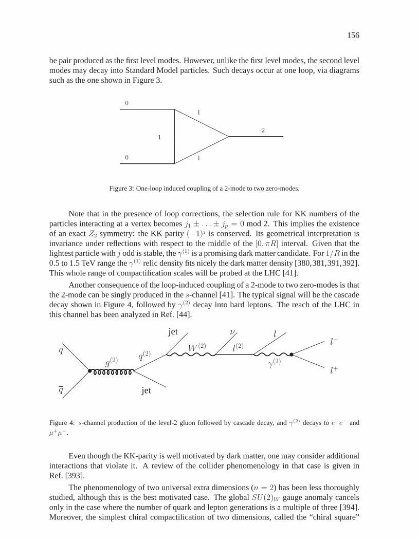
156

be pair produced as the first level modes. However, unlike thefirst level modes, the second levelmodes may decay into Standard Model particles. Such decays occur at one loop, via diagramssuch as the one shown in Figure 3.

HHHHHHHHHH

2

1

1

1

0

0

Figure 3: One-loop induced coupling of a 2-mode to two zero-modes.

Note that in the presence of loop corrections, the selectionrule for KK numbers of theparticles interacting at a vertex becomesj1 ± . . . ± jp = 0 mod 2. This implies the existenceof an exactZ2 symmetry: the KK parity(−1)j is conserved. Its geometrical interpretation isinvariance under reflections with respect to the middle of the [0, πR] interval. Given that thelightest particle withj odd is stable, theγ(1) is a promising dark matter candidate. For1/R in the0.5 to 1.5 TeV range theγ(1) relic density fits nicely the dark matter density [380,381,391,392].This whole range of compactification scales will be probed atthe LHC [41].

Another consequence of the loop-induced coupling of a 2-mode to two zero-modes is thatthe 2-mode can be singly produced in thes-channel [41]. The typical signal will be the cascadedecay shown in Figure 4, followed byγ(2) decay into hard leptons. The reach of the LHC inthis channel has been analyzed in Ref. [44].

@@

@@

@

v

v!!!!!!

aaaaaa

q

q

g(2) q(2)

jet

jet ν l

W (2) l(2)

γ(2)

l−

l+HHHHHH

Figure 4: s-channel production of the level-2 gluon followed by cascade decay, andγ(2) decays toe+e− and

µ+µ−.

Even though the KK-parity is well motivated by dark matter, one may consider additionalinteractions that violate it. A review of the collider phenomenology in that case is given inRef. [393].

The phenomenology of two universal extra dimensions (n = 2) has been less thoroughlystudied, although this is the best motivated case. The global SU(2)W gauge anomaly cancelsonly in the case where the number of quark and lepton generations is a multiple of three [394].Moreover, the simplest chiral compactification of two dimensions, called the “chiral square”

157

[395], preserves a discrete symmetry which is a subgroup of the 6D Lorentz group, such thatproton decay is adequately suppressed even when baryon number is maximally violated at theTeV scale [396].

The Feynman rules for gauge theories in two universal dimensions compactified on thechiral square are given in Ref. [397]. The KK modes are labelled by two KK numbers,(j, k),with j ≥ 1, k ≥ 0. The KK parity of this compactification is(−1)j+k. The gauge bosons in sixdimensions include two scalar fields which are the polarizations along the two extra dimensions.At each KK level, a linear combination of the two scalars is eaten by the spin-1 KK mode, whilethe other linear combination remains as a physical real scalar field. Given that the gauge bosonsbelong to the adjoint representation of the gauge groups, these physical scalars are referred toas “spinless adjoints”. The cross sections for KK pair production are different than in then = 1case due to the presence of the spinless adjoints. The decay modes of the KK states are alsodifferent than in then = 1 case because of the different mass splittings among KK modes. Ofparticular interest are the(1, 1) states, which can be produced in thes-channel and have a massof only

√2/R. The collider phenomenology of two universal extra dimensions is currently

explored [398].

158

Part 24

Kaluza–Klein states at the LHC in modelswith localized fermionsE. Accomando and K. Benakli

AbstractWe give a brief review of some aspects of physics with TeV sizeextra-dimensions. We focus on a minimal model with matter localized at theboundaries for the study of the production of Kaluza-Klein excitationsof gauge bosons. We briefly discuss different ways to depart from thissimple analysis.

1. INTRODUCTION

Despite the remarkable success of the Standard Model (SM) indescribing the physical phe-nomena at the energies probed at present accelerators, someof its theoretical aspects are stillunsatisfactory. One of the lacking parts concerns understanding the gravitational interactionsas they destroy the renormalizability of the theory. Furthermore, these quantum gravity effectsseem to imply the existence of extended objects living in more than four dimensions. This raisesmany questions, as:

Is it possible that our world has more dimensions than those we are aware of? If so, whydon’t we see the other dimensions? Is there a way to detect them?

Of course, the answer to the last question can only come for specific class of models asit depends on the details of the realization of the extra-dimensions and the way known particlesemerge inside them. The examples discussed in this review are the pioneer models describedin Refs. [339, 399–402], when embedded in the complete and consistent framework given in[403,404]. We focus on such a scenario as our aim is to understand the most important conceptsunderlying extra-dimension physics, and not to display a collection of hypothetical models.

Within our framework, two fundamental energy scales play a major role. The first one,Ms = l−1

s , is related to the inner structure of the basic objects of thetheory, that we assume tobe elementary strings. Their point-like behavior is viewedas a low-energy phenomena; aboveMs, the string oscillation modes get excited making their trueextended nature manifest. Thesecond important scale,R−1, is associated with the existence of a higher dimensional space.AboveR−1 new dimensions open up and particles, called Kaluza-Klein (KK) excitations, canpropagate in them.

2. MINIMAL MODELS WITH LOCALIZED FERMIONS

In a pictorial way, gravitons and SM particles can be represented as in Fig. 1. In particular, inthe scenario we consider:

• the gravitons, depicted as closed strings, are seen to propagate in the whole higher-dimensional space, 3+d‖+d⊥. Here, 3+d‖ defines the longitudinal dimension of the bigbrane drawn in Fig. 1, which contains the small 3-dimensional brane where the observed

159

open string

closed string

Extra dimension(s) perp. to the brane

Min

kow

ski 3

+1

dim

ensi

ons

d extra dimensions

||

3+d dimensional brane//3−dimensional brane

A 3−brane inside (intersecting) a 3+d −dimensional brane//

Figure 1: Geometrical representation of models with localized fermions.

SM particles live. The symbold⊥ indicates instead the extra-dimensions, transverse tothe big brane, which are felt only by gravity.

• The SM gauge-bosons, drawn as open strings, can propagate only on the (3+d‖)-brane.• The SM fermions are localized on the 3-dimensional brane, which intersects the (3+d‖)-

dimensional one. They do not propagate on extra-dimensions(neitherd‖ nor d⊥), hencethey do not have KK-excitations.

The number of extra-dimensions,D = d‖,d⊥ or d‖+d⊥, which are compactified on aD-dimensional torus of volumeV = (2π)DR1R2 · · ·RD, can be as big as six [404] or seven [405]dimensions. Assuming periodic conditions on the wave functions along each compact direction,the states propagating in the(4+D)-dimensional space are seen from the four-dimensional pointof view as a tower of states having a squared mass:

M2KK ≡M2

~n = m20 +

n21

R21

+n2

2

R22

+ · · · + n2D

R2D

, (1)

withm0 the four-dimensional mass andni non-negative integers. The states with∑

i ni 6= 0 arecalled KK-states. Assuming that leptons and quarks are localized is quite a distinctive feature ofthis class of models, giving rise to well defined predictions. An immediate consequence of thelocalization is that fermion interactions do not preserve the momenta in the extra-dimensions.One can thus produce single KK-excitations, for example viaf f ′ → V

(n)KK wheref, f ′ are

fermions andV (n)KK represents massive KK-excitations ofW,Z, γ, g gauge-bosons. Conversely,

gauge-boson interactions conserve the internal momenta, making the self-interactions of thekind V V → V

(n)KK forbidden. The experimental bounds on KK-particles that wesummarize in

the following, as well as the discovery potential of the LHC,depend very sensitively on theassumptions made.

Electroweak measurements can place significant limits on the size of the extra-dimensions.KK-excitations might affect low-energy observables through loops. Their mass can thus be con-strained by fits to the electroweak precision data [342,344,406–410]. In particular, the fit to themeasured values ofMW , Γll andΓhad has led toR−1 ≥ 3.6 TeV.

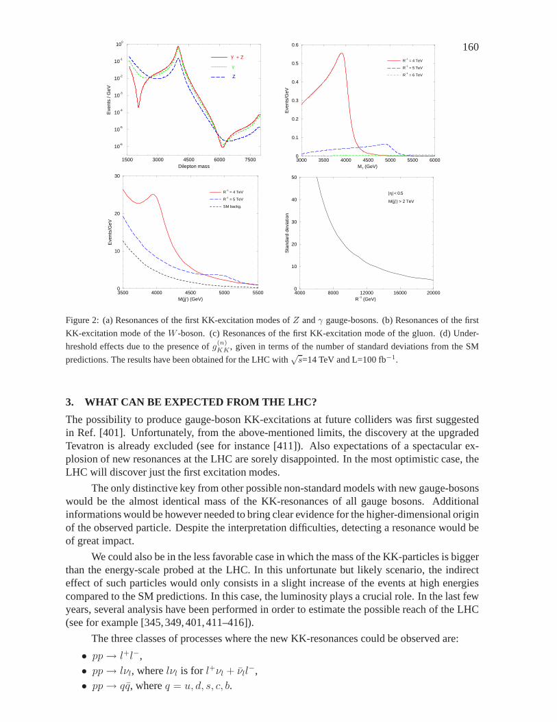
160

1500 3000 4500 6000 7500Dilepton mass

10-6

10-5

10-4

10-3

10-2

10-1

100

Eve

nts

/ GeV

γ + Z

γ

Z

3000 3500 4000 4500 5000 5500 6000MT (GeV)

0

0.1

0.2

0.3

0.4

0.5

0.6

Eve

nts/

GeV

R−1

= 4 TeV

R−1

= 5 TeV

R−1

= 6 TeV

3500 4000 4500 5000 5500M(jj’) (GeV)

0

10

20

30

Eve

nts/

GeV

R−1

= 4 TeV

R−1

= 5 TeV

SM backg.

4000 8000 12000 16000 20000R

−1 (GeV)

0

10

20

30

40

50

Sta

ndar

d de

viat

ion

|η| < 0.5

M(jj’) > 2 TeV

Figure 2: (a) Resonances of the first KK-excitation modes ofZ andγ gauge-bosons. (b) Resonances of the first

KK-excitation mode of theW -boson. (c) Resonances of the first KK-excitation mode of thegluon. (d) Under-

hreshold effects due to the presence ofg(n)KK , given in terms of the number of standard deviations from theSM

predictions. The results have been obtained for the LHC with√s=14 TeV and L=100 fb−1.

3. WHAT CAN BE EXPECTED FROM THE LHC?

The possibility to produce gauge-boson KK-excitations at future colliders was first suggestedin Ref. [401]. Unfortunately, from the above-mentioned limits, the discovery at the upgradedTevatron is already excluded (see for instance [411]). Alsoexpectations of a spectacular ex-plosion of new resonances at the LHC are sorely disappointed. In the most optimistic case, theLHC will discover just the first excitation modes.

The only distinctive key from other possible non-standard models with new gauge-bosonswould be the almost identical mass of the KK-resonances of all gauge bosons. Additionalinformations would be however needed to bring clear evidence for the higher-dimensional originof the observed particle. Despite the interpretation difficulties, detecting a resonance would beof great impact.

We could also be in the less favorable case in which the mass ofthe KK-particles is biggerthan the energy-scale probed at the LHC. In this unfortunatebut likely scenario, the indirecteffect of such particles would only consists in a slight increase of the events at high energiescompared to the SM predictions. In this case, the luminosityplays a crucial role. In the last fewyears, several analysis have been performed in order to estimate the possible reach of the LHC(see for example [345,349,401,411–416]).

The three classes of processes where the new KK-resonances could be observed are:

• pp→ l+l−,• pp→ lνl, wherelνl is for l+νl + νll

−,• pp→ qq, whereq = u, d, s, c, b.

161

The first class can be mediated by the KK-excitations of the electroweak neutral gauge-bosons,Z

(n)KK andγ(n)

KK , while the second one can contain the chargedW(n)KK gauge-boson modes. Finally,

the third class can receive contributions from all electroweak gauge-bosons plus the KK-modesg

(n)KK of the gluons.

Typically, one can expect a kind of signal as given in Fig. 2. In the case where bothoutgoing particles are visible, a natural observable is theinvariant mass of the fermion pair.Distributions in such a variable are shown in the upper and lower left-side plots, which dis-play the interplay betweenZ(n)

KK andγ(n)KK resonances, and the peaking structure due tog

(n)KK ,

respectively. In presence of a neutrino in the final state, one can resort to the transverse massdistribution in order to detect new resonances. This is shown in the upper right-side plot ofFig. 2 for the charged-current process withW (n)

KK exchange. Owing to the PDFs, the effectivecenter-of-mass (CM) energy of the partonic processes available at the LHC is not really high.The discovery limits of the KK-resonances are thus rather modest,R−1 ≤ 5-6 TeV. This esti-mate finds confirmation in more detailed ATLAS and CMS analyses [417]. Taking into accountthe present experimental bounds, there is no much space left. Moreover, the resonances due tothe gluon excitations have quite large widths owing to the strong coupling value. They are thusspread and difficult to detect already for compactification scales of the order of 5 TeV.

But, what represents a weakness in this context can become important for indirect searches.The large width, ranging between the order of a few hundreds GeV for the KK-excitations ofthe electroweak gauge-bosons and the TeV-order for the KK-modes of the gluons, can give riseto sizeable effects even if the mass of the new particles is larger than the typical CM-energyavailable at the LHC. This is illustrated in the lower right-side plot of Fig. 2, where the numberof standard deviations quantifies the discrepancy with the SM predictions, coming fromg(n)

KK

contributions. The under-threshold effects are driven by the tail of the broad Breit-Wigner,which can extend over a region of several TeV, and are dominated by the interference betweenSM and KK amplitudes. They thus require to have non-suppressed SM contributions. Theirsize, of a few-per-cent order for large compactification radii, can become statistically signifi-cant according to the available luminosity. In the extreme case of Fig. 2, we have a KK-gluonwith massM1 = R−1=20 TeV and widthΓ1 ≃2 TeV. Assuming a luminosity L=100fb−1, theinterference terms give rise to an excess of about 2000 events. Similar conclusions hold forthe indirect search of the KK-excitations of the electroweak gauge-bosons. At 95% confidencelevel, the LHC could exclude values of compactification scales up to 12 and 14 TeV from theZ

(n)KK + γ

(n)KK andW (n)

KK channels, respectively. The indirect search is exploited in the ATLASand CMS joint analysis of Ref. [417].

4. GOING BEYOND MINIMAL

We have carried the discussion above for the case of one extra-dimension with all fermionslocalized on the boundaries. One can depart from this simplesituation in many ways:

• More extra-dimensionsNew difficulties arise forD ≥ 2: the sum over KK propagators diverges [399]. A simpleregularization is to cut off the sum of the KK states atMs. This would be natural if theextra-dimension were discrete, however in our model we assumed translation invarianceof the background geometry (before localizing any objects in it). String theory seemsto choose a different regularization [399, 418]. In fact theinteraction ofAµ(x, ~y) =∑

~nAµ~n(x) exp iniyi

Riwith the current densityjµ(x), associated to the massless localized

162

fermions, is described by the effective Lagrangian:∫

d4x∑

~n

e− ln δ

∑

i

n2i l2s

2R2i jµ(x)Aµ

~n(x) , (2)

which can be written after Fourier transformation as∫

d4y

∫

d4x (1

l2s2π ln δ)2e

− ~y2

2l2s ln δ jµ(x)Aµ(x, ~y) . (3)

This means that the localized fermions are felt as a Gaussiandistribution of charge

e−~y2

2σ2 jµ(x) with a width σ =√

ln δ ls ∼ 1.66 ls. Here we usedδ = 16 correspond-ing to aZ2 orbifolding. The couplings of the massive KK-excitations to the localizedfermions are then given by:

g~n =√

2∑

~n

e− ln δ

∑

i

n2i l2s

2R2i g0 (4)

where the factor√

2 stands for the relative normalization of the massive KK wavefunc-tion (cos(niyi

Ri)) with respect to the zero mode, andg0 represents the coupling of the cor-

responding SM gauge-boson.The amplitudes depend on bothR andMs and thus, as phenomenological consequence,all bounds depend on both parameters (see [411]).

• Localized kinetic and/or mass terms for bulk fieldsLet us denote byS0(p, R,Ms) the sum of all tree-level boson propagators weighted by a

factor δ− ~n2

R2M2s from the interaction vertices. For simplicity we takem0 = 0, and define

δS0 by

S0(p, R,Ms) =1

p2+ δS0 . (5)

In order to confront the theory with experiment, it is necessary to include a certain numberof corrections. The obvious one is a resummation of one-loopself-energy correction toreproduce the gauge coupling of the massless vector-bosons. Here we parametrize theseeffects as two kinds of bubbles to be resummed:

– the first, denoted asBbulk represents the bulk corrections. This bubble preserves theKK-momentum,

– the second, denoted asBbdary represents the boundary corrections. This bubble doesnot preserve the KK momentum. In fact, this can represent a boundary mass term ortree-level coupling, but also localized one-loop corrections due to boundary states[399] or induced by bulk states themselves [419].

Here, two simplifications have been made: (a) the corrections are the same for all KK-states, and (b) the boundary corrections arise all from the same boundary. This results inthe corrected propagator [399]:

Scorr(p, R,Ms) =S0

1 − Bbulk − Bbdary − p2δS0Bbdary. (6)

If we define the “renormalized coupling” asg2(p2) = g2

1−Bbulk−Bbdary, the result is

g2Scorr = g2(p2)S0 − δS0g2(1 − p2δS0)Bbdary

(1 − Bbulk − Bbdary)(1 − Bbulk − Bbdaryp2δS0). (7)

163

The first term in Eq.(7) is the contribution that was taken into account in all phenomeno-logical analysis, the second is the correction which depends crucially on the size ofBbdary.

• Spreading interactions in the extra dimensionsIn the simplest scenario, all SM gauge-bosons propagate in the same compact space.However, one may think that the three factors of the SM gauge-group can arise from dif-ferent branes, extended in different compact directions. In this case,d‖ TeV-dimensionsmight be longitudinal to some brane and transverse to others. As a result, only some ofthe gauge-bosons can exhibit KK-excitations. Such a framework is discussed in [411].

These are simplest extensions of the work we presented above. The experimental limits dependnow on many parametersMs,Bbdary, ... in addition to the different size of the compactificationspace felt by the gauge-bosons.

164

Part 25

Kaluza–Klein dark matter: a reviewG. Servant

1. INTRODUCTION

The dominant matter component of our Universe is non-baryonic. The recently publishedWMAP results [3], combined with ACBAR, CBI and 2dFGRS, lead to precise estimates ofthe baryonic, matter and total densities :Ωbh

2 = 0.0224 ± 0.0009, Ωmh2 = 0.135 ± 0.009

andΩtot = 1.02 ± 0.02. One of the most interesting aspects of the dark matter puzzle is thatit is likely to be related to new physics at the TeV scale. Indeed, particles with weak scale sizeinteractions and a mass at the electroweak breaking scale (WIMPs) are typically predicted tohave the good relic density today to account for dark matter,provided that they are stable. Thefavorite WIMP candidate to date is the Lightest Supersymmetric Particle (LSP) and neutralinosare certainly the most extensively studied example.

2. DARK MATTER CANDIDATES FROM EXTRA DIMENSIONS

Alternative models for physics beyond the Standard Model (SM) that make use of extra dimen-sions rather than supersymmetry to solve the gauge hierarchy problem, have been studied inthe last few years. It is now legitimate to ask whether extra dimensions have anything to dowith the dark matter puzzle. Among the new ingredients of extra dimensional theories are theKaluza-Klein (KK) excitations of SM particles as well as theradion, the scalar degree of free-dom related to the size of extra dimensions. If the extra-dimensional model contains branes,there are also possibly branons, which are associated to brane fluctuations. All of them looklike natural candidates for dark matter. Let us start with KKparticles. The idea that they couldform the dark matter is very tempting. However, it turns out that this is not so easy to achieve.Indeed, in most extra-dimensional models, there are no stable KK states, all being able to decayinto SM particles. So the next question is: What are the new symmetries available in extradimensional contexts which could make a KK mode stable? A newdimension means a newconserved momentum along the extra dimension. This leads tothe so-called KK parity, a dis-crete symmetry which remains unbroken in some specific classof extra dimensional modelsnamed Universal Extra Dimensions (UED) [314]. As a result, the Lightest KK particle (LKP)is stable. We can also ask whether there is anything comparable to what happens with super-symmetric dark matter. In this case, the symmetry which guarantees the stability of the LSPhas been primarily postulated to get rid of the proton decay problem in the MSSM. The protondecay problem arises also in extra dimensional theories specifically if the cut-off scale is nearthe TeV scale. It is interesting to investigate whether the symmetry one assumes to get rid of theproton decay can lead to a stable particle, like in susy. We will indeed present such solution inthe context of warped GUT models where the DM particle is called the LZP. The LKP and theLZP are presently the two main proposals for WIMP KK dark matter. We will present them inmore detail in the next sections. Before doing that, let us review other (non-wimp) possibilitieswhich have been mentioned in the literature.

For a particle to be stable, either it has large couplings to SM particles and there must bea symmetry to guarantee its stability– this is the case of wimps like the LSP, the LKP and the

165

LZP which will be presented below– or it interacts so weakly that its lifetime is longer than theage of the universe, this is the case of light particles with only gravitational couplings like theradion in ADD [403] or TeV flat extra dimensions. We go throughthe various possibilities inthe next subsections. The situation is summarized in Table 1.

• radion dark matterm ∼ meVADD models only gravity in bulk • KK graviton dark matterm ∼ meVR ∼ meV−1 (flat) (both finely-tuned)

• branon dark matter(not original ADD, hierarchy pbs remain)

→ gauge bosons in bulk • radion dark matterm ∼ meVTeV−1 dim. (finely-tuned); KK graviton is unstableR ∼ TeV−1 (flat)

• radion dark matterm ∼ meV→ all SM fields in bulk (finely-tuned)“Universal Extra Dimensions” • KK dark matterm ∼ TeV

→ WIMP or SuperWIMP

AdS a la Randall-Sundrum • radion is unstableWarpedgeometries if GUT in the bulk −→ • KK dark matterR ∼M−1

P l m ∼ few GeV–few TeVbutMKK ∼ TeV → WIMP

Table 1: Dark matter candidates in three main classes of extra dimensional models

2.1 KK graviton

2.1.1 In ADD

The KK graviton of ADD, with a meV mass, is stable on cosmological scales (each KK gravitoncouples only with1/MP l) and could be a DM candidate. It would not be a wimp and the correctrelic density cannot be obtained via the standard thermal calculation. To get the correct relicdensity requires fine-tuning either in initial conditions for inflation or in the reheat temperatureof the universe, otherwise, KK gravitons would overclose the universe. In addition, there arestrong astrophysical constraints on the ADD scenario.

2.1.2 In UED: SuperWIMP KK graviton

The situation is different in UED models where the right relic abundance can be obtained nat-urally. The idea is that the standard cold relic abundance isobtained for the next lightest KKparticle (NLKP), which is a WIMP (a KK hypercharge gauge boson in UED with∼TeV mass)and the NLKP later decays into the LKP which is the KK graviton. That way, the KK graviton,which has a TeV mass and only a gravitational coupling can still acquire the right abundance asgiven by the standard thermal relic calculation. This scenario has been intensively studied byFeng et al [420–422].

Finally, let us mention that in Randall-Sundrum models, KK gravitons have a TeV massand interact strongly so they cannot play the role of dark matter.

166

2.2 Radion

The radion in ADD has typically the same mass and same coupling as the KK graviton andalso suffers from an overclosure problem. As for models withTeV extra dimensions, there isalso typically an overclosure problem. Solving it requiresmodifying the assumptions on thecompactification scheme. Details of radion cosmology have been studied in [423]. The radionoverclosure problem does not apply in Randall-Sundrum where the radion has large interactionsand large mass so that it decays fast.

2.3 Branons

Branons correspond to brane fluctuations. They control the coordinate position of our branein the extra dimensions.Those fields can be understood as thegoldstone boson arising fromspontaneous breaking of translational invariance by the presence of the brane. They get massiveby the explicit breaking of the symmetry. The possibility that branons could be dark matter hasbeen investigated in [424,425]. In this context, the SM lives on a 3D brane embedded in a higherdimensional (D=4+N) space-time where the fundamental scale of gravityMD is lower than thePlanck scale. In the original ADD proposal,MD was the TeV scale. The authors of branon darkmatter work in a general brane world scenario with arbitraryfundamental scale (larger than theTeV scale). The branon degree of freedom cannot be neglectedwhen the brane tension scalefis much smaller thanMD, which means that we live on a non rigid brane. Branon interactionswith particles living on the brane can be computed as a function of f , N and the branon massM . Couplings of KK modes to the fields confined on the brane are exponentially suppressedby the fluctuation of the brane [426]. Asf is very small, the KK mode contributions becomeinvisible from our world and the only remaining degrees of freedom are the branons. Thegravitational interaction on the brane conserves parity and terms in the effective Lagrangian withan odd number of branons are forbidden. As a consequence, branons are stable. Constraintsin the region of parameters made byN , MD, M andf have been derived. We refer the readerto [424,425] for details and references.

2.4 KK “photon”

As it will be presented in the next section, in the class of models with Universal Extra Dimen-sions [314], the Lightest KK Particle (LKP) is stable. For∼TeV−1 sized extra dimensions, theLKP can act as a WIMP. It was identified as the first KK excitation of the photon. To be precise,it is not really a KK photon because the Weinberg angle for KK modes is very small [348]. Itis essentially the KK hypercharge gauge boson:B(1). Relic density [380, 381, 392, 427, 428],direct [391, 429] and indirect detection [391, 430–435] studies of this candidate have all beencarried out in the last few years. Constraints on these models from radion cosmology have alsobeen studied [423].

2.5 KK neutrino

The possibility that the LKP is a KKνL rather than a KK photon in UED was also studiedin [381, 429]. This case is excluded experimentally by direct detection experiments because ofthe large coupling ofν(1)

L to the Z gauge boson, leading to much too large elastic scattering ofthe KK neutrino with nucleons.

It could also be that the LKP is the KK excitation of a RH neutrino. To behave as a WIMP,such particle should interact with TeV KK gauge bosons like in Left Right gauge theories such

167

as Pati-Salam orSO(10). This possibility was investigated in details in the context of warpedgeometries and more specifically in the context of warped Grand Unified Theories (GUTs)[382,436]. It will be presented in section 4..

To summarize, so far, KK particles arise as stable viable WIMPs in two frameworks : InUniversal Extra Dimensions and in some warped geometries ala Randall-Sundrum. We willdiscuss these two possibilities in more details now.

3. THE LKP IN UNIVERSAL EXTRA DIMENSIONS

In models with Universal Extra Dimensions (UED) [314] whichare explained earlier in theseproceedings, all SM fields propagate in flat toroidal extra dimensions, unlike models with LargeExtra Dimensions a la ADD. Translation invariance along anextra dimension is only brokenby the orbifold imposed to recover a chiral SM spectrum. Still, there is a remnant discretesymmetry called KK parity,(−1)n, wheren is the KK number. This symmetry insures thatinteraction vertices cannot involve an odd number of odd-KKstates and, therefore, a vertexwith two SM particles (withn = 0) and one KK state (withn = 1) is forbidden. As a result,the Lightest KK Particle (LKP) withn = 1 cannot decay into SM particles and is stable. Notethat for KK parity to be an exact symmetry, one has to assume that the boundary lagrangians atthe two orbifold fixed points are symmetric.

In contrast with supersymmetry where the mass spectrum is largely spread so that atmost a few additional particles participate in coannihilation processes with the LSP, in MinimalUED (MUED), the mass spectrum of KK particles is rather degenerate and there are manycoannihilation processes. The KK mass splittings are essentially due to radiative corrections.Those were computed in [348]. The spectrum of KK masses depends also on the values ofboundary terms at the cut-off scale, which are not fixed by known SM physics. In this sense,the values of the KK masses can be taken arbitrary and the UED scenario has a multitude ofparameters. The authors of [348] assumed that the boundary terms vanish (this is the so-calledMUED hypothesis). In this case, the LKP is the KK hyperchargegauge bosonB(1).

The viability and relic density of the LKP were first analyzedin [381] with some sim-plifying assumption about the KK spectrum. Only one co-annihilation channel was considered(involving the KK right-handed electron). Ref. [380, 392] include all coannihilation channelswith KK fermions and KK gauge bosons and look at the effect of each channel separately. Thenet result is that even if the new coannihilations are Boltzmann suppressed their effect is stillsignificant because the cross sections are mediated by weak or strong interactions while thecross sections studied so far were purely hypercharge-mediated processes. Their conclusionis that in MUED, the LKP mass should be within 500-600 GeV while in non-minimal UEDmodels, freedom in the KK mass spectrum allows an LKP as heavyas 2 TeV. For an analysistaking into account the effects of second level KK modes see [427, 428]. The effect of coan-nihilation with the KK Higgs was studied in [437]. Shortly after the appearance of [380, 392],Ref. [438] came out where they derive a strong constraint on the KK scale of MUED modelsfrom precision EW observables (> 700 GeV)14. This seems to exclude MUED KK dark matterbut KK dark matter survives in non-minimal UED models, wherethe KK mass can be as largeas 2 TeV.

To conclude this section, note that the cases where the LKP isa KK Z or KK H remain14Previous bounds on 1/R from EW precision tests were derived in [314, 439], from direct non-detection and

from b→ sγ in [440] and from FCNC in [441,442].

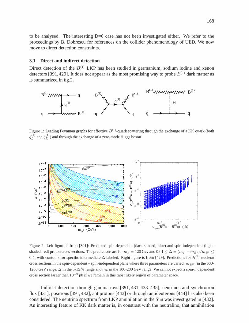
168

to be analysed. The interesting D=6 case has not been investigated either. We refer to theproceedings by B. Dobrescu for references on the collider phenomenology of UED. We nowmove to direct detection constraints.

3.1 Direct and indirect detection

Direct detection of theB(1) LKP has been studied in germanium, sodium iodine and xenondetectors [391,429]. It does not appear as the most promising way to probeB(1) dark matter asis summarized in fig.2.

q

B(1)

q(1)

B(1)

q

q

B(1)

q(1)

q

B(1)

q

B(1)

H

B(1)

q

Figure 1: Leading Feynman graphs for effectiveB(1)-quark scattering through the exchange of a KK quark (both

q(1)L andq(1)R ) and through the exchange of a zero-mode Higgs boson.

10-12

10-11

10-10

10-9

10-8

10-7

10-6

10-5

σspin(B(1)n → B(1)n) (pb)

σ S(B

(1) n

→ B

(1) n)

(p

b)

Figure 2: Left figure is from [391]: Predicted spin-dependent (dark-shaded, blue) and spin-independent (light-

shaded, red) proton cross sections. The predictions are formh = 120 Gev and0.01 ≤ ∆ = (mq1 −mB1)/mB1 ≤0.5, with contours for specific intermediate∆ labeled. Right figure is from [429]: Predictions forB(1)-nucleon

cross sections in the spin-dependent – spin-independent plane where three parameters are varied:mB(1) in the 600-

1200 GeV range,∆ in the 5-15% range andmh in the 100-200 GeV range. We cannot expect a spin-independent

cross section larger than10−9 pb if we remain in this most likely region of parameter space.

Indirect detection through gamma-rays [391, 431, 433–435], neutrinos and synchrotronflux [431], positrons [391,432], antiprotons [443] or through antideuterons [444] has also beenconsidered. The neutrino spectrum from LKP annihilation inthe Sun was investigated in [432].An interesting feature of KK dark matter is, in constrast with the neutralino, that annihilation

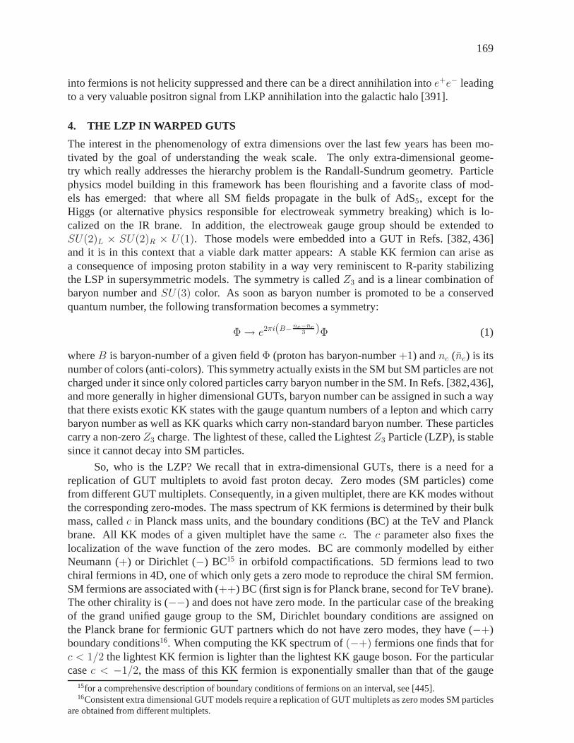
169

into fermions is not helicity suppressed and there can be a direct annihilation intoe+e− leadingto a very valuable positron signal from LKP annihilation into the galactic halo [391].

4. THE LZP IN WARPED GUTS

The interest in the phenomenology of extra dimensions over the last few years has been mo-tivated by the goal of understanding the weak scale. The onlyextra-dimensional geome-try which really addresses the hierarchy problem is the Randall-Sundrum geometry. Particlephysics model building in this framework has been flourishing and a favorite class of mod-els has emerged: that where all SM fields propagate in the bulkof AdS5, except for theHiggs (or alternative physics responsible for electroweaksymmetry breaking) which is lo-calized on the IR brane. In addition, the electroweak gauge group should be extended toSU(2)L × SU(2)R × U(1). Those models were embedded into a GUT in Refs. [382, 436]and it is in this context that a viable dark matter appears: A stable KK fermion can arise asa consequence of imposing proton stability in a way very reminiscent to R-parity stabilizingthe LSP in supersymmetric models. The symmetry is calledZ3 and is a linear combination ofbaryon number andSU(3) color. As soon as baryon number is promoted to be a conservedquantum number, the following transformation becomes a symmetry:

Φ → e2πi(B−nc−nc3 )Φ (1)

whereB is baryon-number of a given fieldΦ (proton has baryon-number+1) andnc (nc) is itsnumber of colors (anti-colors). This symmetry actually exists in the SM but SM particles are notcharged under it since only colored particles carry baryon number in the SM. In Refs. [382,436],and more generally in higher dimensional GUTs, baryon number can be assigned in such a waythat there exists exotic KK states with the gauge quantum numbers of a lepton and which carrybaryon number as well as KK quarks which carry non-standard baryon number. These particlescarry a non-zeroZ3 charge. The lightest of these, called the LightestZ3 Particle (LZP), is stablesince it cannot decay into SM particles.

So, who is the LZP? We recall that in extra-dimensional GUTs,there is a need for areplication of GUT multiplets to avoid fast proton decay. Zero modes (SM particles) comefrom different GUT multiplets. Consequently, in a given multiplet, there are KK modes withoutthe corresponding zero-modes. The mass spectrum of KK fermions is determined by their bulkmass, calledc in Planck mass units, and the boundary conditions (BC) at theTeV and Planckbrane. All KK modes of a given multiplet have the samec. The c parameter also fixes thelocalization of the wave function of the zero modes. BC are commonly modelled by eitherNeumann (+) or Dirichlet (−) BC15 in orbifold compactifications. 5D fermions lead to twochiral fermions in 4D, one of which only gets a zero mode to reproduce the chiral SM fermion.SM fermions are associated with (++) BC (first sign is for Planck brane, second for TeV brane).The other chirality is (−−) and does not have zero mode. In the particular case of the breakingof the grand unified gauge group to the SM, Dirichlet boundaryconditions are assigned onthe Planck brane for fermionic GUT partners which do not havezero modes, they have (−+)boundary conditions16. When computing the KK spectrum of(−+) fermions one finds that forc < 1/2 the lightest KK fermion is lighter than the lightest KK gaugeboson. For the particularcasec < −1/2, the mass of this KK fermion is exponentially smaller than that of the gauge

15for a comprehensive description of boundary conditions of fermions on an interval, see [445].16Consistent extra dimensional GUT models require a replication of GUT multiplets as zero modes SM particles

are obtained from different multiplets.

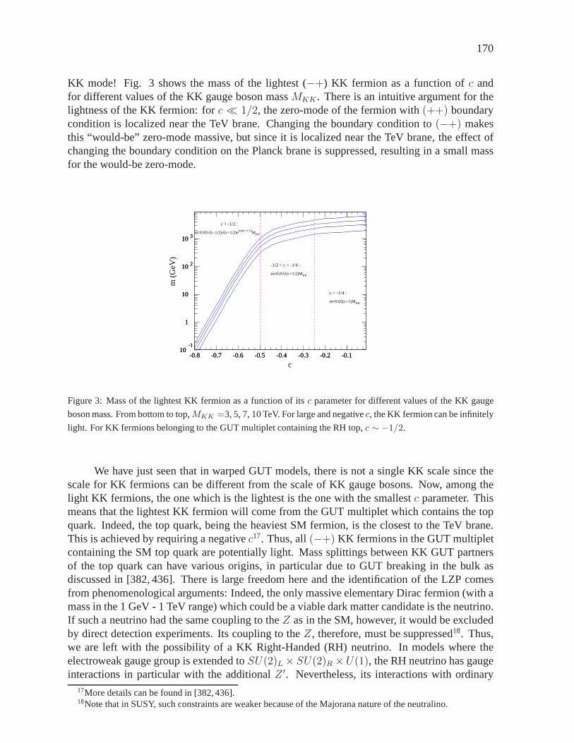
170

KK mode! Fig. 3 shows the mass of the lightest (−+) KK fermion as a function ofc andfor different values of the KK gauge boson massMKK . There is an intuitive argument for thelightness of the KK fermion: forc ≪ 1/2, the zero-mode of the fermion with(++) boundarycondition is localized near the TeV brane. Changing the boundary condition to(−+) makesthis “would-be” zero-mode massive, but since it is localized near the TeV brane, the effect ofchanging the boundary condition on the Planck brane is suppressed, resulting in a small massfor the would-be zero-mode.

10-1

1

10

10 2

10 3

-0.8 -0.7 -0.6 -0.5 -0.4 -0.3 -0.2 -0.110

-1

1

10

10 2

10 3

-0.8 -0.7 -0.6 -0.5 -0.4 -0.3 -0.2 -0.1

c < -1/2 :

m≈0.83√(c-1/2)√(c+1/2)ekπr(c+1/2)MKK

-1/2 < c < -1/4 :

m≈0.83√(c+1/2)MKK

c > -1/4 :

m≈0.65(c+1)MKK

c

m (

GeV

)

Figure 3: Mass of the lightest KK fermion as a function of itsc parameter for different values of the KK gauge

boson mass. From bottom to top,MKK =3, 5, 7, 10 TeV. For large and negativec, the KK fermion can be infinitely

light. For KK fermions belonging to the GUT multiplet containing the RH top,c ∼ −1/2.

We have just seen that in warped GUT models, there is not a single KK scale since thescale for KK fermions can be different from the scale of KK gauge bosons. Now, among thelight KK fermions, the one which is the lightest is the one with the smallestc parameter. Thismeans that the lightest KK fermion will come from the GUT multiplet which contains the topquark. Indeed, the top quark, being the heaviest SM fermion,is the closest to the TeV brane.This is achieved by requiring a negativec17. Thus, all(−+) KK fermions in the GUT multipletcontaining the SM top quark are potentially light. Mass splittings between KK GUT partnersof the top quark can have various origins, in particular due to GUT breaking in the bulk asdiscussed in [382, 436]. There is large freedom here and the identification of the LZP comesfrom phenomenological arguments: Indeed, the only massiveelementary Dirac fermion (with amass in the 1 GeV - 1 TeV range) which could be a viable dark matter candidate is the neutrino.If such a neutrino had the same coupling to theZ as in the SM, however, it would be excludedby direct detection experiments. Its coupling to theZ, therefore, must be suppressed18. Thus,we are left with the possibility of a KK Right-Handed (RH) neutrino. In models where theelectroweak gauge group is extended toSU(2)L× SU(2)R ×U(1), the RH neutrino has gaugeinteractions in particular with the additionalZ ′. Nevertheless, its interactions with ordinary

17More details can be found in [382,436].18Note that in SUSY, such constraints are weaker because of theMajorana nature of the neutralino.

171

matter are feeble because they involve the additional gaugebosons which have a large mass(MKK ∼> 3 TeV). This opens the possibility of a weakly interacting Dirac RH neutrino. Inprinciple, the LZP is not necessarily the lightest KK particle. There might be lighter KK modesbut which are unstable because they are not charged underZ3. In practise though, and in themodels of [382,436], the RH neutrino LZP turns out to be the lightest KK particle due to variousphenomenological constraints.

In summary, the LZP is a Kaluza–Klein fermion, which is a four-component spinor andvector-like object. As explained in great detail in Ref. [382], it can be naturally very light, muchlighter than the KK scale of Randall-Sundrum models, namelyMKK ∼> 3 TeV. This is becausethe RH chirality is localized near the TeV brane while the LH one is near the Planck brane.The overlap of wave functions is small, resulting in a small Dirac KK mass. Its lightness isrelated to the top quark’s heaviness but not entirely fixed byit, so that LZPs in the mass rangeof approximately 20 GeV to a few TeV can be considered. We refer to the LZP as if it were achiral fermion because only the RH chirality has significantinteractions and the other chiralitydecouples. In addition, the LZP has the same gauge quantum numbers as the RH neutrino ofSO(10) or Pati–Salam. As a result, we refer to it as a “Dirac RH neutrino”.

Via the AdS/CFT correspondence, the Randall-Sundrum scenario is dual to a 4D compos-ite Higgs scenario, in which the unification of gauge couplings has recently been studied [446].In this case, the LZP maps to some low-lying hadron at the composite scale. We also point outthat in Refs. [382, 436], the strong coupling scale is close to the curvature scale so thatO(1)variations in calculations are expected. Results of [382, 436] should therefore be considered asrepresentative rather than a complete description.

4.1 Relic Density

An interesting feature of warped GUT models is that GUT states such asX, Y gauge bosonsappear at the TeV scale (via the KK excitations). InSO(10), there are also theX ′, Y ′, Xs, Z ′,etc. that the LZP can couple to. The LZP couples to the TeV KK gauge bosons ofSO(10). Inaddition, when electroweak symmetry is broken,Z − Z ′ mixing induces a coupling of the RHneutrino to the SMZ gauge boson. This coupling is suppressed by(MZ/MZ′)2. If MZ′ ∼ fewTeV (the mass of KK gauge bosons is set byMKK), the size of this coupling will typically beideal for a WIMP. There is actually a second source for theZ-LZP coupling, which we will notdiscuss here but refer the reader to Ref. [382] for a detailedexplanation. The point is that thereis enough freedom in the model under consideration to treat the LZP-Z coupling as an almostarbitrary parameter.

For LZPs lighter than approximately 100 GeV, LZP annihilations proceed dominantlyvia s-channelZ-exchange and annihilations to light quarks, neutrinos andcharged leptons areimportant. For larger masses, annihilation via the t-channel exchange ofXs into top quarksor via s-channelZ ′ exchange intott, bb, W+W− andZh dominates. LZPs can generate theobserved quantity of dark matter thermally in two mass ranges: near theZ-resonance (mLZP ≈35-50 GeV) and for considerably heavier masses (mLZP ∼> several hundred GeV) [382, 436].Several approximations were made in the relic density calculation of [382, 436], like using thenon-relativistic expansion, neglecting the annihilationvia s-channel Higgs exchange as wellas co-annihilation with KKτ ′R . A more precise calculation is being carried out using theCOMPHEP model for warped GUTs and associated with MICROMEGAS [447].

Annihilations can vary from one Dirac RH neutrino dark matter model to another, depend-ing on whether, at large LZP mass, annihilations take place via s-channelZ ′ exchange only or

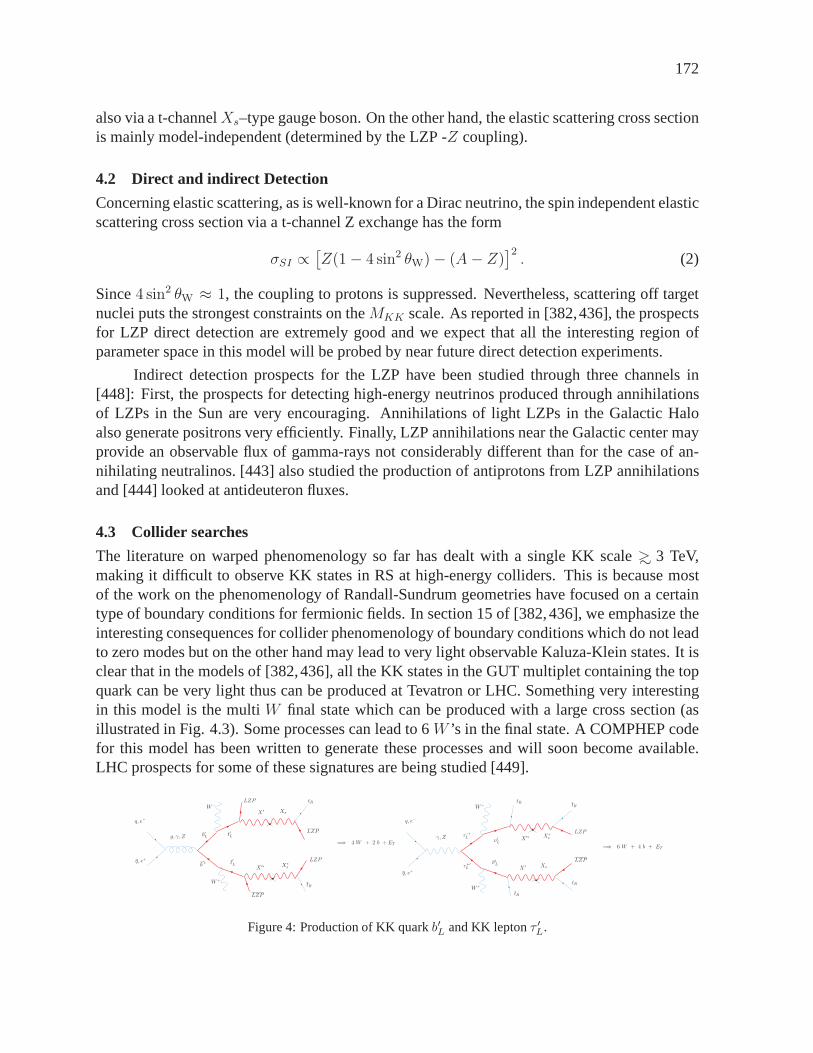
172

also via a t-channelXs–type gauge boson. On the other hand, the elastic scatteringcross sectionis mainly model-independent (determined by the LZP -Z coupling).

4.2 Direct and indirect Detection

Concerning elastic scattering, as is well-known for a Diracneutrino, the spin independent elasticscattering cross section via a t-channel Z exchange has the form

σSI ∝[Z(1 − 4 sin2 θW) − (A− Z)

]2. (2)

Since4 sin2 θW ≈ 1, the coupling to protons is suppressed. Nevertheless, scattering off targetnuclei puts the strongest constraints on theMKK scale. As reported in [382,436], the prospectsfor LZP direct detection are extremely good and we expect that all the interesting region ofparameter space in this model will be probed by near future direct detection experiments.

Indirect detection prospects for the LZP have been studied through three channels in[448]: First, the prospects for detecting high-energy neutrinos produced through annihilationsof LZPs in the Sun are very encouraging. Annihilations of light LZPs in the Galactic Haloalso generate positrons very efficiently. Finally, LZP annihilations near the Galactic center mayprovide an observable flux of gamma-rays not considerably different than for the case of an-nihilating neutralinos. [443] also studied the productionof antiprotons from LZP annihilationsand [444] looked at antideuteron fluxes.

4.3 Collider searches

The literature on warped phenomenology so far has dealt witha single KK scale∼> 3 TeV,making it difficult to observe KK states in RS at high-energy colliders. This is because mostof the work on the phenomenology of Randall-Sundrum geometries have focused on a certaintype of boundary conditions for fermionic fields. In section15 of [382,436], we emphasize theinteresting consequences for collider phenomenology of boundary conditions which do not leadto zero modes but on the other hand may lead to very light observable Kaluza-Klein states. It isclear that in the models of [382,436], all the KK states in theGUT multiplet containing the topquark can be very light thus can be produced at Tevatron or LHC. Something very interestingin this model is the multiW final state which can be produced with a large cross section (asillustrated in Fig. 4.3). Some processes can lead to 6W ’s in the final state. A COMPHEP codefor this model has been written to generate these processes and will soon become available.LHC prospects for some of these signatures are being studied[449].

W−

W+

b′L

b′L t

′L

LZP

LZP

t′L

X ′ Xs

X ′∗ X∗s

tR

LZP

LZP

tR

=⇒ 4 W + 2 b + ET

q, e−

q, e+

g, γ, Z τ−′L

τ+′L

W+

W−

ν ′L

ν ′L

tR

X ′∗ X∗s

tR

LZP

LZP

tR

XsX ′

tR

q, e−

q, e+

=⇒ 6 W + 4 b + ET

γ, Z

Figure 4: Production of KK quarkb′L and KK leptonτ ′L.

173

5. COMPARISONS BETWEEN THE LSP, LKP ad LZP

Table 2 gives a brief comparison of the LSP, LKP and LZP. For a more detailed comparison,see the last section of [448].

LKP LZP LSP

Set up Universal Extra Dimensions Warped GUTs SUSY

Nature of Gauge boson Dirac fermion Majorana fermiondark matter particle

KK parity: consequence of Z3: imposed R-parity: imposedSymmetry geometry if ones assumes to protect to protect

equal boundary lagrangians proton stability proton stability

(−1)n B − nc − nc3

(−1)3(B−L)+2S

Mass range ∼ 600-1000 GeV 20 GeV-few TeV ∼ 50 GeV-1 TeV

Annihilation cross s-wave s-wave p-wavesection into fermions helicity-suppressed

Favourite detection •LHC •Direct detection •LHC•Indirect detection •LHC

•Indirect detection

Table 2: Comparison between the wimp dark matter candidatesdiscussed in this review.

6. CONCLUSION

Alternatives to SUSY dark matter exist and viable examples arise from extra dimensional mod-els. Because of their simplicity, models with Universal Extra Dimensions have attracted muchattention. The Minimal UED (MUED) model is an ideal benchmark model and a good startingpoint as far as the testability of extra dimensional models is concerned. Discriminating betweenMUED and SUSY at colliders is an active field of study. Most of the interest in UED is dueto the possibility of a stable KK particle and in particular to the LKP as dark matter. Directand indirect detection of the LKP have been investigated. Onthe other hand, UED do not par-ticularly solve the hierarchy problem. Extra dimensional models with warped geometry do so.Among the Randall-Sundrum realizations, those with the SM fields living in the bulk are themost appealing. In this framework, the EW sector is extendedtoSU(2)L×SU(2)R×U(1). Inthis report, we have reviewed a GUT embedding of this gauge structure, which we believe leadsto a very rich and peculiar phenomenology. For instance, it is possible that the symmetry im-posed to prevent proton decay leads to a stable KK particle which can act as dark matter. Notethat independently from the existence of a stable KK mode, warped GUTs possess interestingfeatures and there is still a lot to be done as far as phenomenological exploration of RS modelswith SM in the bulk is concerned.

174

Part 26

The Higgs boson as a gauge fieldG. Cacciapaglia

AbstractThe Higgs boson in the SM is responsible for the breaking of the elec-troweak symmetry. However, its potential is unstable underradiativecorrections. A very elegant mechanism to protect it is to usegaugesymmetry itself: it is possible in extra dimensional theories, where thecomponents of gauge bosons along the extra direction play the role ofspecial scalars. We discuss two different attempts to builda realisticmodel featuring this mechanism. The first example is based ona flatextra dimension: in this case the Higgs potential is completely finiteand calculable. However, both the Higgs mass and the scale ofnewphysics result generically too light. Nevertheless, we describe two pos-sible approaches to solve this problem and build a realisticmodel. Thesecond possibility is to use a warped space, and realize the Higgs asa composite scalar. In this case, the Higgs and resonances are heavyenough, however the model is constrained by electroweak precision ob-servables.

1. INTRODUCTION

In the Standard Model of particle physics, the breaking of the electroweak symmetry is gener-ated by a scalar field, the Higgs. The minimal Higgs sector consists of a doublet of the weakSU(2)L: a suitable potential for such scalar will induce a vacuum expectation value for it thatwill break the gauge symmetry and give a mass both to the weak gauge bosons, theW andZ,and to the matter fermions. This description is very successful from the experimental point ofview: even though we do not have direct measurements in this sector, precision tests of the SMseem to be consistent with the presence of a relatively lightHiggs, with mass between115 GeVand∼ 300 GeV. The lower bound comes from direct searches at LEP, whilethe upper boundcomes from the loop effects of the Higgs to precision observables [450].

Notwithstanding this success, the Higgs mechanism is stillunsatisfactory from a theoret-ical point of view. First of all, the potential is somehow putby hand and is not calculable forthe Higgs boson is not protected by any symmetry. Moreover, from an effective theory point ofview, the potential is unstable: loop corrections will induce a dependence on some new physicsthat appears at high energies. For instance, the mass term isquadratically sensitive to such newphysics scale: the bounds on the Higgs mass would require this scale to be around1 TeV. Thisscale is much lower that the expected UV scales, like the Planck mass where quantum gravitybecomes relevant, at1016 TeV, or Grand Unification scales, around1011 ÷ 1013 TeV. Unlessa huge fine tuning is advocated, the SM contains a hierarchy between such scales. Moreover,building a model with new physics at a TeV is very difficult, because of bounds coming fromprecision observables: higher order operators, that will generically be generated by such newphysics, pose a bound on the new physics scale around5 ÷ 10 TeV 19 [451].

19This bound comes from universal operators. Bounds from flavour violating terms require a higher scale,

175

A very appealing idea, utilizing extra dimensions, is to identify the Higgs boson as thecomponent along some extra spatial dimension of a gauge boson, and it was first proposed inRefs. [452–454]. In this way, the symmetry breaking does notcome from a fundamental scalarof the theory, thus improving the stability of the mechanism. Moreover, gauge invariance in theextra dimensional theory will highly constrain the potential, forbidding for instance a mass term.Now, the loop contributions to the mass term will be insensitive to the cutoff of the theory, thusto the UV physics, and they may be responsible for EWSB. The crucial point here is that suchcontributions are finite and calculable! Due to gauge invariance itself, the EW scale will also beprotected with respect to the UV cutoff. The simplest possibility is to work in 5 dimensions: inthis case there is only one extra component

AM = (Aµ, A5) . (1)

The minimal requirements on the bulk gauge groupG is that it has to contain the SM gaugegroupG ∈ SU(2)L×U(1)Y , and a doublet of SU(2)L, to be identified with the Higgs, is embed-ded in the adjoint representation. The gauge groupG is broken by an orbifold projection to theSM oneH assigning different parities (or boundary conditions) to the gauge bosons of differentgenerators. This corresponds to20

Aaµ(−y) = Aaµ(y) if a ∈ H ,Abµ(−y) = −Abµ(y) if b ∈ G/H .

(2)

For theA5 component, 5D Lorentz invariance imposes opposite parities. Thus, there is a zeromode only along the broken generators: these are the only physical scalars in the spectrum,as all the massive modes ofA5 can be gauged away, and will play the role of the longitudinalmodes of the massive vector bosons. In other words, the Higgsdoublet has to be contained inAb5. The gauge transformations, at linear level, reads:

Aµ → Aµ + ∂µλ(x, x5) + i[λ(x, x5), Aµ] , (3)

A5 → A5 + ∂5λ(x, x5) + i[λ(x, x5), A5] . (4)

This symmetry is enough to ensure that it is not possible to write down a tree level potential forA5 in the bulk. Indeed, the only invariant is the energy stress tensor

FMN = ∂MAN − ∂NAM + ig[AM , AN ] ; (5)

being antisymmetric,F55 = 0. The situation is more subtle on the fixed points of the orbifold:the gauge transformation parameterλ, has the same parities of the gauge fieldsAµ. Thus, forthe broken generators,λ is odd: this means that on the fixed pointx⋆

Ab5(x⋆) → Ab5(x⋆) + ∂5λb(x⋆). (6)

This incomplete gauge transformation, however, is enough to forbid a potential localized on thefixed points.

This argument can be generalized to more extra dimensions. The first difference is thata potential is allowed by gauge invariance: indeed,Fij , wherei and j are along the extradimensions, is gauge invariant. In particular a quartic term may be generated at tree level.

around100 ÷ 1000 TeV.20This is the simplest possibilities. A more general set of orbifold projections has been studied in Ref. [455].

176

However, it is generically possible to write a linear term inthe energy stress tensor on thefixed points: this will generate tadpoles for the scalars, sothat one has to choose the orbifoldprojection in order to forbid them [456,457].

While this mechanism offers great simplicity and elegance,building a realistic model isvery difficult. The main problems are the lightness of the Higgs and of the top quark. Regardingthe top, the Yukawas are generated via the gauge coupling itself, so it is generically hard to engi-neer a Yukawa of order 1 from a small gauge coupling. Regarding the Higgs mass, it turns out tobe too small, below the value currently excluded by LEP, because the quartic scalar interactionterm is generated at one loop. Since the entire potential (mass and quartic) is loop generated, thepotential will also generically prefer large values of the Higgs vacuum expectation value (VEV)relative to the compactification scale so that the scale of new physics stays dangerously low.It is interesting to note that a deconstructed version of this mechanism [458] led to the idea ofLittle Higgs models. The symmetry protecting the Higgs massis now a discrete shift symmetry,and the construction is much less constrained by the absenceof 5D Lorentz invariance. In LittleHiggs models, this idea has been pushed further: in this casethe symmetry is protecting theHiggs mass at one loop, but allows a quartic coupling at tree level [459].

Several models, both in 5 (see Refs. [460–466]) and 6 (see Refs. [467–469]) dimen-sions have been proposed in the literature, in the context offlat extra dimensions. Anotherinteresting development is to embed the same idea in a warpedextra dimension [470] as inRefs. [446,471–473]. The nice thing is that the warping enhances both the Higgs and top mass.However, the non trivial background will also induce corrections to electroweak precision ob-servables that constitute the strongest constraint on thismodels. Interestingly, a correspondencefist developed in the string context allows to relate these theories to 4 dimensional ones, inparticular to strongly coupled conformal theories (CFTs),where conformality is broken at theresonance scale. From this point of view, the Higgs is a composite particle of the CFT, like inthe Georgi-Kaplan theories in Refs. [474–477].

In the next sections we will briefly discuss the main featuresand differences of modelsin flat and warped space. For simplicity we will focus on two simple examples, nice for theirsimplicity and minimality: the SU(3)w model in 5D of Ref. [463] in flat space, and the minimalcomposite Higgs model of Ref. [472]. However, the properties highlighted here are common toall the models proposed in the literature.

2. FLAT SPACE

As already mentioned above, we need to embed the SM electroweak gauge group, SU(2)L×U(1)Y ,into a larger bulk gauge group, that contains a doublet of SU(2) in the adjoint representation.This group is broken to the SM one by an orbifold projection: in this way, at energies belowthe compactification scale, only the SM gauge symmetry is unbroken. A more general breakingof the symmetry can be achieved using boundary conditions: however in the following we willinsist on the orbifold projection. The reason is the absenceof tree level corrections to elec-troweak precision observables: in this case, a zero mode like theW andZ is orthogonal to allthe massive KK modes of other fields. If the Higgs vev is constant along the extra dimension,as it is the case in flat space, it will not induce mixings between the zero modes and the KKmodes: this is the source of universal corrections. If the symmetry breaking is not given byan orbifold parity, but by boundary conditions, the orthogonality argument does not work anymore. We will comment more on this issue later.

The simplest choice is to enlarge the weak group to SU(3)w, and break it to SU(2)L×U(1)Y

177

on the orbifoldS1/Z2: an analysis of all the rank 2 groups can be found in Ref. [468]. The ad-joint of SU(3) decomposes into (3, 0) + (2, 1/2) + (2, -1/2) + (1, 0). After the orbifold projection,the only (massless) scalar left in the theory is a complex doublet with hypercharge1/2, that weidentify with the SM HiggsH5. As already mentioned, this scalar will not have any potential attree level: however, loops will induce a potential that is insensitive to the UV cutoff, and thuscalculable. For the moment we will assume that such potential will induce a VEV for the Higgs,thus breaking the electroweak symmetry. We can use SU(2) transformations to align the VEV,analogously to the SM case, and parametrize it

〈H5〉 =√

2

(0

α/R

)

. (7)

It is now straightforward to compute the spectrum of the gauge bosons: we find

MWn =n+ α

R, MZn =

n+ 2α

R, Mγn =

n

R, (8)

wheren ∈ Z, and we want to identify the lightest state in each tower withthe SM gauge bosons,the photon, theW and theZ. Let us first point out that the spectrum is invariant if we shift α byan integer, and if we change its sign. In other words, the physical range forα is [0, 1/2] and allother vacua outside this range are equivalent, as the radiatively induced potential will respect thesame symmetries. Another important feature is thatMZ turns out to be twice theW mass: thisis a consequence of the gauge group SU(3) that predictsθW = π/3. One possible way to fix it isto add localized gauge kinetic terms: SU(3) being broken on the boundaries, such terms can bedifferent for the SU(2) and U(1) and, if large enough, can dominate and fix the correct value ofsin θW . However, this scenario is equivalent to a warped extra dimension: integrating out a sliceof the warped space near the Planck brane, where the warping is small, will mimic the localizedkinetic terms, while the remaining space will be almost flat.We will discuss the warped case inthe next section: the main drawback is that it suffers from tree level corrections to the precisionobservables [473]. Another possibility is to extend the gauge group with an extra U(1)X . Inthis case, if the bulk fermions are charged, only the combination of the two U(1)’s proportionalto the hypercharge is anomaly free, and the orthogonal gaugeboson will develop a mass [467].Alternatively, one can use boundary conditions to break U(1)w×U(1)X → U(1)Y , for instanceby twisting the BC on one of the two branes, such that no zero mode is left in the scalar sector21.

The next problem is how to generate a mass for the SM matter fields. If we added bulkfermions, with chiral zero modes thanks to the orbifold projection, the Higgs VEV would gen-erate a spectrum similar to that in (8): all the light modes would have masses larger than theWmass, where the exact relation depends on group theory factors arising from the fermion repre-sentations. Indeed, gauge invariance forces the Higgs to couple to bulk fields and with strengthdetermined by the 5D gauge couplingg5. There are two possible solutions: one is to includeodd masses for these fermions, that will localize the zero modes toward the two fixed points.As modes with different chirality will be localized toward different points, this mechanism willreduce the overlaps between the wave functions, and generate hierarchies between the variousYukawa couplings. Another possibility, adopted in [456, 468] is to localize the SM fermionson the fixed points, and then mix them with massive bulk fields that will induce an effectiveYukawa couplinga la Froggatt-Nielsen. In this case, the mass for the light fermions can be

21Note however that these breaking mechanisms will reintroduce tree level oblique corrections, see Refs. [465,466]

178

given either by small mixings, or by a large bulk mass that will exponentially suppress the ef-fective Yukawa. In the latter case, with order 1 masses, it ispossible to explain the hierarchiesin the Yukawa sector [456,466]. The flavour structure of the theory for the first two generationshas been studied in Ref. [478].

The main problem in the fermion sector is then how to explain the heaviness of the top:indeed a bulk field will generically couple to the Higgs with the gauge coupling, predicting afermion mass of ordermW . A possible way to fit the top is to embed it in a large representation,such that the effective Yukawa is enhanced by a group theory factor. This possibility has beenexploited in Ref. [465]: the authors find that the minimal representation of SU(3)w is a symmet-ric 15. This choice would predictmt = 2mW at tree level: QCD corrections might enhance thepole mass to a realistic value. The main drawback of this possibility is that the largish represen-tation will lower the scale where the extra dimensional theory becomes strongly coupled. Forthe 15, using Naive Dimensional Analysis, we can estimate such scale to 2 ÷ 3 × 1/R. More-over, the presence of a triplet of SU(2) in the decompositionof the 15 will introduce tree levelcorrection to the coupling of thebl with theZ. Such corrections come from the mixing with thezero mode of the triplet and not from the effect of the KK modes. Removing the zero mode witha localized mass will induce mixing with the KK modes: this corrections can be translated into abound on the compactification scale1/R > 4÷5 TeV. Another possibility pursued in Ref. [466]is to explicitly break Lorentz invariance along the extra dimension. In this case, each fermionwill effectively feel a different length, thus removing therelation between the top and theWmasses. The strong coupling scale is also lowered, but in a less dramatic way. However, in thiscase, the Lorentz breaking will induce a UV cutoff sensitivity in the Higgs potential at higherloop level. In Ref. [466] the authors focus their attention on the flavour problem: again cor-rections toZblbl and 4 fermion operators induced from the gauge boson resonances [407, 479]pose a bound on the scale1/R of few TeV.

Once the field content in the bulk is specified, it is possible to compute the Higgs potentialas it is finite. Their spectrum, as a function of the Higgs VEVα, generically takes the form:

m2n = M2 +

(n+ ξα)2

R2, n ∈ Z , (9)

whereξ is determined by the representation of the field. We can use the Higgs-dependentspectrum to compute the full one-loop potential, using the Coleman-Weinberg formula: aftersumming over the KK modes [467], we find

Veff(α) =∓1

32π2

1

(πR)4Fκ(α) , (10)

where the signs stand for bosons/fermions and

Fκ(α) =3

2

∞∑

n=1

e−κn cos(2πξαn)

n3

(κ2

3+κ

n+

1

n2

)

, (11)

whereκ = 2πMR. The contribution of fields with large bulk mass is exponentially suppressed.Moreover, the leading contribution is given by

± cos 2πξα . (12)

While bosons will not break the gauge symmetry, the fermion contribution will induce a VEV

αmin =1

2ξ. (13)

179

From the formula for theW mass it follows that the compactification scale is given by

1

R= 2ξmW . (14)

Thus, generically the mass of the resonances is too low, unless a very large representationis included in the theory, thus lowering the strong couplingscale to unacceptable values. Apossible way out is to consider cancellations between different bulk fields: it would be crucialto have fields that give a positive contribution to the Higgs mass, like a boson. A scalar would beradiatively unstable, however a bulk fermion with twisted boundary conditions, or anti periodicalong the extra dimension, will have the same effect [462, 464]. Indeed, the spectrum is givenby

m2n = M2 +

(n+ 1/2 + ξα)2

R2, n ∈ Z . (15)

The contribution to the effective potential is given by the previous formulas, withξα → ξα +1/2. As

cos(2πn(ξα+ 1/2)) = (−1)n cos(2πnξα) ,

the twisted parity approximately flips the overall sign of the contribution. In this way, we canget positive contributions to the Higgs mass arising from fermions. In Ref. [465], the authorspropose a minimal model where such cancellation does occur:they only consider bulk fermionsthat give mass to the third generations. The presence of twisted fermions ensures that the scale1/R can be naturally raised up to∼ 20mW , without a parametric fine tuning.

Another generic problem is the value of the Higgs mass: beingthe potential loop induced,it is loop suppressed with respect to theW mass. However, the presence of several bulk fermionsis enough to raise it above the direct LEP bound. In the model of Ref. [465], the fermionsassociated with the third generation are enough to push the Higgs mass up to∼ 150 GeV, theprecise value depending on the choice of representations. In the Lorentz violating model ofRef. [466], the same mechanism enhancing the top mass works for the Higgs: in other words,the Higgs mass is set by the scale of the top resonances, and not the gauge boson ones. In thisway, Higgses as heavy as few hundred GeV are possible.

A final comment regards the bounds on the scale1/R in this kind of models. As alreadymentioned, the flatness of the Higgs VEV generically ensuresthe absence of tree level universalcorrections, because it does not mix the bulk zero modes withthe KK resonances. However,such corrections will be introduced back by large terms localized on the fixed points, that havethe phenomenologically important role of getting rid of unwanted zero modes left over after theorbifold projection. In the specific model we discuss here, the triplet in the top15 correctsZbb,and the extra U(1) induces aρ parameter and further corrections toZbb [465]. Such correctionsbound1/R > 4 ÷ 5 TeV, thus requiring a moderate fine tuning in the potential. Anothersimilar bound comes from four fermion operators, induced bythe coupling of the localizedlight fermions with the KK resonances [407, 479]: however, this bound depends on the lightgenerations, that do not play a crucial role in the electroweak symmetry breaking mechanism.

3. WARPED SPACE: A COMPOSITE HIGGS

A different approach to the one described in the above section is to work with a warped extradimension, like the one described by Randall and Sundrum in Ref. [470]. The metric is not a

180

trivial extension of Minkowski, but can be written in a conformal way as

ds2 =1

(kz)2

(dxµdx

µ − dz2), (16)

where the extra coordinatez ranges in the interval[L0, L1]. The meaning of the warping isclear: the unit length defined byds2, or alternatively the energy scale, depends on the positionalong the extra dimension. IfL0 ∼ 1/k, then the energy scale on the endpointL1 is reduced(warped) by a factor ofkL1. Generically, the scalek ∼ 1/L0 is taken to be equal to the cutoffof the theory, usually the Planck mass, while the scale1/L1 is of order the electroweak scale.This setup allows to explain geometrically the large hierarchy between the two scales [470].

A very interesting aspect of this background is the presenceof a duality, conjectured instring theory [480–483], that draws a correspondence with a4 dimensional theory: we willvery briefly sketch the main properties of this 4D theory, that will be useful to illustrate the5D model building. This theory is a strongly coupled conformal field theory (CFT), where theconformality is broken at a scaleµIR: this means that the spectrum will contain a tower ofweakly coupled “mesons” with masses proportional to such scale. We can also add elementaryfields, external to the conformal sector, and couple them with the strongly coupled sector. Theidea is that the SM gauge bosons and fermions22 are the elementary fields, and the breaking ofthe electroweak symmetry is generated by the quasi-conformal sector: in other words, the Higgsis a composite state of the strong sector, like in the models presented by Georgi and Kaplan inRefs [474–477]. The holographic dual of this theory is a theory defined on a RS background:the elementary fields are the values of the 5D fields on theL0 brane, that we will call Planckbrane. In particular, the gauge symmetries of the elementary sector will be the only unbrokengauge groups on the Planck brane. On the other hand, the global symmetries of the conformalsector are translated into gauge symmetries in the bulk and on theL1 brane, the TeV brane. ThescaleµIR where conformality is broken, corresponds to the warped energy scale on the TeVbrane. The two theories are equivalent, meaning that they share the same physical properties:the only advantage of the 5D interpretation is that it is weakly coupled, up to a scale a fewtimes higher thatµIR, and some properties, like the composite Higgs potential and VEV, arecalculable.

Another advantage of using a warped space is that both the Higgs and top masses areenhanced with respect to the flat case. The Higgs VEV profile along the extra dimension isdetermined by the geometry, and in this case it will be linearin the coordinatez. This meansthat a field localized toward the TeV brane has a larger overlap with the Higgs, thus its massis enhanced. As a consequence, the top has to live near the TeVbrane, thus being a compositestate in the 4D interpretation. However, the non trivial profile for the Higgs VEV also generatesmixing between zero modes and KK modes, in the 4D language between the elementary fieldsand the composite states. These mixings will induce corrections to the couplings with fermionsat tree level, in particular oblique and non oblique corrections. Thus, EWPT will be the strongestbound on the parameter space of this theory. The third generation also plays an important role:the heaviness of the top requires it to be a composite state. However, this will also imply largedeviations in the couplings of bottom and top with the weak gauge bosons. TheZbb couplingand loop corrections to theρ parameter coming from the mass splitting between top and bottomwill also severely constrain the model.

A model of warped Gauge-Higgs unification was proposed in Ref. [472]. The SM weak22The top will be the only exception, as we will see.

181

gauge group is extended to a SO(5)w×U(1)B−L in the bulk. It is broken to the SM SU(2)L×U(1)Yon the Planck brane, such that the SM gauge bosons are indeed fields external to the CFT. Onthe TeV brane SO(5) is broken to SO(4)∼ SU(2)L×SU(2)R. The adjoint representation of thebulk group will contain a 4 of SO(4), namely a complex bidoublet of SU(2)L×SU(2)R: thescalar zero mode arising from theA5 component is then identified with the SM Higgs boson. Itis crucial the presence of a custodial symmetry in the bulk and TeV brane [484]: in the 4D inter-pretation it means that the CFT sector is invariant, so it will not induce large corrections to theρparameter at tree level, ensuring the correct relation between theW andZ masses. Fermions areadded as complete SO(5) representations, one for each SM fermion, and boundary conditionswill select a zero mode only for the component with the correct quantum numbers23. A massterm in the bulk controls the localization of such zero modes, thus the overlap with the HiggsVEV. The more localized on the Planck brane, the smaller the effective Yukawa coupling: inthis way it is possible to generate the hierarchies in the fermion yukawa sector [485, 486]. The4D interpretation makes this behaviour more clear: the light fields are elementary fields witha small mixing with the composite sector, that couples directly with the Higgs boson [487].However, the heaviness of the top requires that at least the right-handed part is a composite,thus localized on the TeV brane.

Once the field content is specified, it is possible to compute exactly the potential forthe Higgs [472]. The leading contributions are given bysin and cos functions, and can beparametrized as:

V (h) ∼ α cosh

fπ− β sin2 h

fπ, (17)

whereh is the Higgs field,fπ is the decay constant of the CFT resonances, in the 5D languagefπ = 2/

√

g25k 1/L1. TheW mass is given by:

MW =g2

2v2 , where v = ǫfπ = fπ sin

< h >

fπ= 246GeV. (18)

The parameterǫ is crucial in these models: it controls the size of the extra dimensionL1 interms of the SM weak scale, and the size of the tree level corrections. Using the approximateformula in Eq. 17, it is given by:

ǫ ∼

√

1 −(α

2β

)2

, (19)

thus in order to have a small VEV with respect to the new physics scalefπ some fine tuning inthe potential is required, as in the flat case. The corrections to electroweak precision observableswill also depend onǫ thus constraining its size:S ∼ ǫ2, T ∼ ǫ6, while from the third generationδgZblbl ∼ ǫ2, T1-loop ∼ ǫ2. The precise bound onǫ depends on other parameters, especiallythe ones involved in the third generation sector. A very detailed analysis has been performedin Ref. [473]: they find that universal corrections only requires ǫ ≤ 0.4 ÷ 0.5, values that canbe obtained without any significant fine tuning in the potential. However, if one includes theconstraints from the third generation, bothZbb and loop corrections toρ, ǫ ≤ 0.2 is required.Such corrections might be removed if the third generation isintroduced in a non minimal way,as discussed in Ref. [473].

23the BCs impose the vanishing of some components on the end pointsL0 andL1. These BCs are equivalent tothe orbifold parities used in the flat case. Components without a zero mode are like the anti periodic fermions.

182

An interesting prediction of this model is the lightness of the Higgs. In all the numericalexamples studied in Ref. [473] the authors findmH ≤ 140 GeV. Moreover, the model predictsthe presence of resonances of gauge bosons and fermions at a scale that depends from the valueof ǫ: it can be as low as2 TeV if the bounds from the third generation are removed, thusbeingaccessible at LHC. However, the corrections toZbb constrain the new particles above4 TeV.Thus model also contains a nice feature: unification of the 3 SM gauge couplings at a levelcomparable to the supersymmetric model [446]. This featuredoes not depend on the details ofthe strong sector, but only to the composite nature of the Higgs and the right-handed top.

4. CONCLUSIONS

We have described a mechanism that protects the Higgs potential from divergent radiative cor-rections using the gauge symmetry in extra dimensions. The Higgs is indeed the component ofa gauge field along the extra direction. After the orbifold breaking, a shift symmetry will highlyconstrain the potential at tree level, ensuring its finiteness. In particular, in the presence of onlyone extra dimension, the potential is completely radiativeand calculable. The presence of bulkfermions will then induce a non trivial minimum and thus drive electroweak symmetry break-ing. In the literature, two main direction has been pursued:flat and warped extra dimensions.The nice property of the flat background is that the Higgs VEV is constant in the extra coordi-nate, thus potentially avoiding tree level corrections to precision observables coming from themixing between KK levels. However, it is generically hard toget a realistic spectrum: the scaleof new physics results too light, and the Higgs and top massesare too small. A possible way toenhance the scale1/R is to allow cancellations in the potential, using anti periodic fermions: inthis way, scales above a TeV scan be obtained without fine tuning. To enhance the top mass, itis possible either to embed it into a largish representationof the bulk gauge group, or to breakexplicitly the Lorentz invariance along the extra dimension. This also allows to get a heavyenough top. In the warped case, the distorted background enhance the masses naturally, viadifferent wave function overlaps. However, the Higgs VEV isnot flat anymore and tree levelcorrections will bound the model. In both cases, the size of the extra dimension, i.e. the scale ofthe KK resonances, is constrained to be larger that4÷ 5 TeV, thus being unobservable at LHC.

Acknowledgements

This research is supported by the NSF grant PHY-0355005.

183

Part 27

Little Higgs models: a Mini-ReviewM. Perelstein

1. INTRODUCTION

In this contribution, we will review the Little Higgs (LH) models, an interesting new class of the-ories of electroweak symmetry breaking (EWSB) that recently attracted considerable attention.While these models do not involve new dimensions of space, the key insight that led to theirconstruction, the “collective symmetry breaking” mechanism, was gleaned by Arkani-Hamed,Cohen and Georgi [458] from a study of five-dimensional theories through the application ofthe dimensional deconstruction approach [488].

Precision electroweak data prefer a light Higgs boson:mh<∼ 245 GeV at 95% c.l., as-

suming no other new physics [48]. A satisfactory theory of EWSB must contain a mechanismto stabilize the Higgs mass against radiative corrections.One intriguing possibility is that theHiggs is a composite particle, a bound state of more fundamental constituents held together bya new strong force [474, 489]. This scenario relates the weakscale to the confinement scaleof the new strong interactions, which is generated via dimensional transmutation and can benaturally hierarchically smaller than the Planck scale. However, since precision electroweakdata rule out new strong interactions at scales below about 10 TeV, an additional mechanismis required to stabilize the “little hierarchy” between theHiggs mass and the strong interactionscale. In analogy with the pions of QCD, the lightness of the Higgs could be explained if it werea Nambu-Goldstone boson(NGB) corresponding to a spontaneously broken global symmetryof the new strongly interacting sector. Gauge and Yukawa couplings of the Higgs, as well as itsself-coupling, must violate the global symmetry explicitly: an exact NGB only has derivativeinteractions. Quantum effects involving these interactions generate a mass term for the Higgs.In a generic model, the dominant effect comes from one-loop quadratically divergent part of theColeman-Weinberg (CW) potential, and its large size makes the models phenomenologicallyunacceptable: either the Higgs is too heavy to fit the data, orthe strong coupling scale is toolow. Little Higgs models avoid this difficulty by incorporating the collective symmetry breakingmechanism, which enforces the cancellation of the quadratically divergent one-loop contribu-tions to the Higgs mass, making a light composite Higgs compatible with the 10 TeV stronginteraction scale. The cancellation is due to a set of new TeV-scale particles (typically gaugebosons and vector-like quarks) predicted by the LH models. If these models are realized in na-ture, the LHC experiments should be able to discover these particles and study their propertiesextensively.

2. LITTLEST HIGGS MODEL

Many LH models have been proposed in the literature; as an example, let us briefly review the”Littlest Higgs” model [459], which provides one of the mosteconomical implementations ofthe idea and forms the basis for most phenomenological analyses. Consider a model with anSU(5) global symmetry, spontaneously broken down to anSO(5) subgroup, at a scalef ∼ 1

184

TeV, by a vacuum condensate in the symmetric tensor representation:

Σ0 =

0 0 110 1 011 0 0

, (1)

where11 is a 2×2 identity matrix. The model contains 14 massless NGB fieldsπa, one foreach broken generatorXa. At energy scales belowΛ ∼ 4πf , the NGB interactions are inde-pendent of the details of the physics giving rise to the condensate and can be described by anSU(5)/SO(5) non-linear sigma model (nlσm), in terms of the sigma fieldΣ(x) = e2iΠ/fΣ0,whereΠ =

∑

a πa(x)Xa. An [SU(2) × U(1)]2 subgroup of theSU(5) is weakly gauged. The

gauged generators are embedded in such a way that gauging each SU(2) × U(1) factor leavesanSU(3) subgroup of the global symmetry unbroken:

Qa1 =

σa/2 0 00 0 00 0 0

, Qa2 =

0 0 00 0 00 0 −σa∗/2

,

Y1 = diag(3, 3,−2,−2,−2)/10 , Y2 = diag(2, 2, 2,−3,−3)/10 . (2)

At the scalef , the condensateΣ0 breaks the full gauge group down to the diagonalSU(2) ×U(1), identified with the SM electroweak group. Four gauge bosons,W±

H ,W3H andBH , acquire

TeV-scale masses by absorbing four of the NGB fields. The remaining NGBs decompose into aweak doublet, identified with the SM HiggsH, and a weak tripletΦ:

Π =

∗ H ΦH† ∗ HT

Φ H∗ ∗

, (3)

where asterisks denote eaten fields. At the quantum level, gauge interactions induce a Coleman-Weinberg potential for the NGBs. However, the Higgs is embedded in such a way that thesubset of global symmetries preserved by eachSU(2) × U(1) gauge factor would be sufficientto ensure the exact vanishing of its potential. Both gauge factors, acting collectively, are neededto break enough symmetry to induce a non-zero CW potential for H: any diagram contributingto this potential must involve at least one power of a gauge coupling from each factor. Oneloop diagrams satisfying this criterion are at most logarithmically divergent; the usual one-loop quadratic divergence in the Higgs mass does not appear.The same collective symmetrybreaking approach can be used to eliminate the large contribution to the Higgs mass from thetop quark loops: the top Yukawa arises from two terms in the Lagrangian, each of which byitself preserves enough global symmetry to keep the Higgs exactly massless. Implementing thisidea requires the introduction of a new vector-like fermion, theT quark, with massmT ∼ f andthe quantum numbers of the SMtR. It is interesting that, in contrast to SUSY, the cancellationsin the LH model involve particles ofthe same spin: the divergence due to the SM top loop iscancelled byT loops, while the divergence due to the SM gauge bosons is cancelled by theloops ofWH andBH . The leading contribution to the CW potential from top loopshas the form

m2h = −3

λ2tm

2T

8π2log

Λ2

m2T

, (4)

and has the correct sign to trigger EWSB. The contributions from gauge and scalar loops havethe opposite sign, but are typically smaller than (4) due to the large top Yukawa; the two-loop contributions are subdominant. The tripletΦ is not protected by the collective symmetry

185

breaking mechanism, and acquires a TeV-scale mass at one loop. AnH†ΦH coupling is alsogenerated at this scale, producing an order-one Higgs quartic coupling whenΦ is integrated out.Thus, the model provides an attractive picture of radiativeEWSB, with the required hierarchiesv ∼ f/(4π) ∼ Λ/(4π)2 emerging naturally.

The Littlest Higgs model is remarkably predictive, describing the TeV-scale new physicswith only a small number of free parameters. The model contains twoSU(2) gauge couplings,two U(1) couplings, and two couplings in the top Yukawa sector; however, in each case, onecombination of the two is fixed by the requirement to reproduce the SMg, g′, andyt. Thisleaves three independent parameters; it is convenient to use three mixing angles,ψ, ψ′, andα,respectively. These angles, along with the scalef , determine the masses and couplings of thenew states; for example,

M(WH) =g

sin 2ψf , M(BH) =

g′√5 sin 2ψ′

f , M(T ) =

√2λt

sin 2αf. (5)

Two additional parameters, coefficientsa anda′ from the quadratically divergent part of theone-loop CW potential, are required to describe the weak triplet sector.

3. LITTLEST HIGGS PHENOMENOLOGY

The LH model succeeded in pushing the strong coupling scale up to the phenomenologicallyacceptable values around 10 TeV, at the expense of introducing new particles at the TeV scale.The presence of these particles affects precision electroweak observables, and their propertiesare constrained by data. These constraints have been workedout in detail in Refs. [490–493]and in Refs. [232, 494, 495] where the constraints from LEP2 experiments have been included.Unfortunately, it was found that the simplest version of themodel outlined above is stronglydisfavored by data: the symmetry breaking scale is bounded by f > 4 TeV at 95% c.l. inthe “best-case” scenario, and the bound is even stronger forgeneric parameters. Such a highf would require a substantial amount of fine tuning to maintainthe lightness of the Higgs,largely destroying the original motivation for the LH model. The corrections to observables arepredominantly generated by the tree-level exchanges of heavy gauge bosons and the non-zerovacuum expectation value (vev) of the weak tripletΦ; both these effects violate the custodialSU(2) symmetry. The gauge boson contribution is dominated by theBH , whose mass is typi-cally well below the scalef , see Eq. (5). The simplest way to alleviate the situation is to reducethe gauge group toSU(2) × SU(2) × U(1)Y , abandoning the collective symmetry breakingmechanism in theU(1) sector. This eliminates theBH boson, and consistent fits forf as low as1 TeV can be obtained [496,497], albeit only in a rather smallregion of the parameter space asshown in Fig. 1. Due to the small value of the SMU(1)Y coupling, the uncanceled contributionto the Higgs mass from this sector does not introduce significant fine tuning.

The study of the LHC signatures of the Littlest Higgs model has been initiated in Refs. [497–499]; a detailed study including realistic detector simulations has been subsequently performedby the ATLAS collaboration [500]. In the preferred parameter range, the heavySU(2) gaugebosonsW±

H andW 3H are expected to be copiously produced at the LHC by the Drell-Yan pro-

cess. Their decays into lepton pairs provide a very clear signature, with the reach in this channelextending toM(WH) ≈ 5 TeV for typical parameters (see Fig. 2). Other decay channels in-clude quark pairs, which could be used to test the universality of theWH couplings to thefermions predicted by the model, as well as gauge boson and gauge boson-Higgs pairs, e.g.

186

Figure 1: Contour plot of the allowed values off in theSU(5)/SO(5) Littlest Higgs model with anSU(2) ×SU(2) × U(1) gauged subgroup, as a function of the parametersc ≡ cos θ anda. The gray shaded region at the

bottom is excluded by requiring a positive triplet mass. From Ref. [496].

W 3H → W+W−, Zh. The latter channels are extremely interesting because theLH model

makes a clean prediction for their branching ratios,

Br(W 3H → Zh) = Br(W 3

H →W+W−) =cot2 2ψ

2 cotψBr(W 3

H → ℓ+ℓ−). (6)

This prediction is a direct consequence of the collective symmetry breaking mechanism, andcan be used to probe this mechanism experimentally [499, 501]. This requires an independentmeasurement of the mixing angleψ, which can be obtained from theWH production crosssection if its mass is known. The prediction can also be tested with high precision at the ILC,even running below theWH production threshold [502].

TheT quark can be pair-produced viaqq, gg → T T , or singly produced viaWb → T .For most of the relevant parameter range, energy is at a premium and the single productiondominates. The decays of theT can be understood using the Goldstone boson equivalencetheorem: in theMT ≫ v limit, it is easy to show that

Γ(T → th) = Γ(T → tZ0) =1

2Γ(T → bW+) =

λ2TMT

64π, (7)

whereλT = λt tanα. Additional decay modes, involving the TeV-scale gauge bosons of theLittlest Higgs model, may be kinematically allowed and contribute to the totalT width: forexample, if theBH boson is present and light, the decayT → tBH may be possible. All threeSM decay modes in Eq. (7)provide characteristic signaturesfor the discovery of theT at theLHC. A detailed study of the LHC discovery potential in each decay mode has been preformedby the ATLAS collaboration [500]. TheWb signal, reconstructed via theℓνb final state, wasfound to be the most promising, with the5σ discovery reach of 2000 (2500) GeV fortanα = 1(2) and 300 fb−1 integrated luminosity. TheZt channel, reconstructed using leptonicZ decays

187

Figure 2: Accessible regions, in theM(WH)− cotψ plane, for5σ discovery at the LHC with 300 fb−1 integrated

luminosity. From Ref. [500].

andt → Wb → ℓνb, provides a clean signature with small backgrounds, as shown in Fig. 3.However, the discovery reach is somewhat below that for theWbmode due to smaller statistics:1050 (1400) GeV withtanα = 1 (2) and 300 fb−1. Theht mode is more challenging, but iftheT quark is observed in other channels and its mass is known, theht signal can be separatedfrom background and used to check the decay pattern in Eq. (7). The cancellation of one-loopdivergences in the LH model hinges on the relation

mT

f=λ2t + λ2

T

λT. (8)

Once theT quark is discovered, a measurement of its mass and production cross section, to-gether with the determination off from the study of theWH bosons, can be used to test therelation [497].

4. LITTLEST HIGGS WITH T PARITY

While reducing the gauge group provides one possible solution to the difficulty experiencedby the Littlest Higgs model in fitting the electroweak data, amore elegant solution has beenproposed by Cheng and Low [503, 504]. They enlarge the symmetry structure of the modelsby introducing an additional discrete symmetry, dubbed “T parity” in analogy to R parity inthe minimal supersymmetric standard model (MSSM). T paritycan be implemented in any LHmodels based on a product gauge group, including the Littlest Higgs [505]. The parity explicitlyforbids any tree-level contribution from the heavy gauge bosons to the observables involvingonly SM particles as external states. It also forbids the interactions that induce the triplet vev. Asa result, corrections to precision electroweak observables are generated exclusively at loop level,

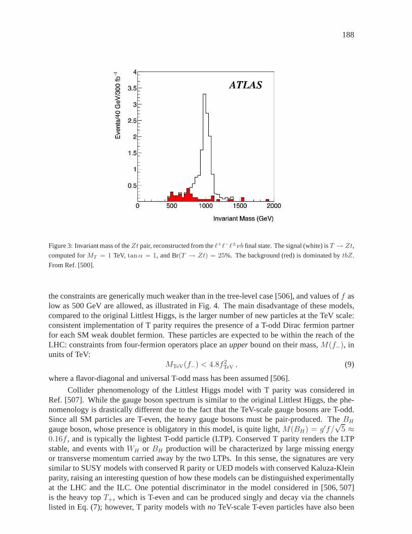
188

Figure 3: Invariant mass of theZt pair, reconstructed from theℓ+ℓ−ℓ±νb final state. The signal (white) isT → Zt,

computed forMT = 1 TeV, tanα = 1, and Br(T → Zt) = 25%. The background (red) is dominated bytbZ.

From Ref. [500].

the constraints are generically much weaker than in the tree-level case [506], and values off aslow as 500 GeV are allowed, as illustrated in Fig. 4. The main disadvantage of these models,compared to the original Littlest Higgs, is the larger number of new particles at the TeV scale:consistent implementation of T parity requires the presence of a T-odd Dirac fermion partnerfor each SM weak doublet fermion. These particles are expected to be within the reach of theLHC: constraints from four-fermion operators place anupperbound on their mass,M(f−), inunits of TeV:

MTeV(f−) < 4.8f 2TeV , (9)

where a flavor-diagonal and universal T-odd mass has been assumed [506].

Collider phenomenology of the Littlest Higgs model with T parity was considered inRef. [507]. While the gauge boson spectrum is similar to the original Littlest Higgs, the phe-nomenology is drastically different due to the fact that theTeV-scale gauge bosons are T-odd.Since all SM particles are T-even, the heavy gauge bosons must be pair-produced. TheBH

gauge boson, whose presence is obligatory in this model, is quite light,M(BH) = g′f/√

5 ≈0.16f , and is typically the lightest T-odd particle (LTP). Conserved T parity renders the LTPstable, and events withWH or BH production will be characterized by large missing energyor transverse momentum carried away by the two LTPs. In this sense, the signatures are verysimilar to SUSY models with conserved R parity or UED models with conserved Kaluza-Kleinparity, raising an interesting question of how these modelscan be distinguished experimentallyat the LHC and the ILC. One potential discriminator in the model considered in [506, 507]is the heavy topT+, which is T-even and can be produced singly and decay via the channelslisted in Eq. (7); however, T parity models withno TeV-scale T-even particles have also been

189

Figure 4: Exclusion contours in terms of the parameterR ≡ tanα and the symmetry breaking scalef , in the

Littlest Higgs model with T parity. In the left panel, the contribution of the T-odd fermions is neglected; in the

right panel, this contribution is included assuming that ithas the maximal size consistent with the constraint from

four-fermion interactions, Eq. (9). From Ref. [506].

constructed [508].

In analogy to SUSY neutralino, the stable LTP can play the role of a weak scale darkmatter candidate, providing additional motivation for themodels with T parity [507,509].

5. OTHER LITTLE HIGGS MODELS

Starting with the “moose” model of Ref. [458], many models ofEWSB incorporating the col-lective symmetry breaking mechanism have been constructed. These can be divided into twoclasses: the “product-group” models, including the Littlest Higgs along with the models inRefs. [510–513], and the “simple-group” models of Refs. [514–516]. The salient phenomeno-logical features of models within the same class are expected to be similar [501]. The simplestsimple-group model, theSU(3) model of [514], embeds the Higgs into an[SU(3)/SU(2)]2

non-linear sigma model, with anSU(3) × U(1) gauged subgroup broken down to the SMSU(2)×U(1) at low energies. At the TeV scale, the model contains a set of five gauge bosons,X±, Y 0

1,2, andZ ′, as well as a large number of new fermions, since all SM doublets need to beextended to complete representations of theSU(3) group. Precision electroweak constraints onthis model and its[SU(4)/SU(3)]4 extension have been considered in Refs. [496, 515]. TheLHC phenomenology of theSU(3) model has been studied in Ref. [501], which also outlinedthe measurements which would need to be performed to discriminate between the product-groupand simple-group models.

The non-linear sigma models of the LH theories break down at the 10 TeV scale, andneed to be supplemented by a more fundamental description. Such description can involve newstrongly coupled physics [517, 518], but may also be weakly coupled [519]. However, it isunlikely that the LHC experiments will be able to discern thephysics beyond the nlσm.

190

6. CONCLUSIONS

In this chapter, we have briefly reviewed the Little Higgs models, which provide an attractivescenario combining dynamical stabilization of the weak-Planck hierarchy by dimensional trans-mutation with the radiative EWSB. We concentrated on the Littlest Higgs model, two versionsof which (a model with a single gaugedU(1) factor and a T-parity symmetric model) provideacceptable fits to precision electroweak data without significant fine tuning. The models makeinteresting predictions which can be tested at the LHC. Morework is required in order to ensurethat the LHC experiments maximize their potential in searching for the predicted signatures; tothis end, it would be useful to systematically incorporate the LH model into the standard MonteCarlo packages such asPYTHIA andHERWIG.

Due to length limitations, many aspects of Little Higgs model-building and phenomenol-ogy could not be covered in this section; for more information and a comprehensive collectionof references, we refer the interested reader to the recent review articles [520,521].

Acknowledgements

This research is supported by the NSF grant PHY-0355005.

191

Part 28

Testing the Littlest Higgs model inΦ++

pair production at LHCA. Hektor, M. Kadastik, K. Kannike, M. Muntel and M. Raidal

AbstractMotivated by predictions of the littlest Higgs model, we carry out aMonte Carlo study of doubly charged Higgs pair production ina typ-ical LHC experiment. We assume additionally that triplet Higgs alsogenerates the observed neutrino masses which fixes theΦ++ leptonicbranching ratios. This allows to test neutrino mass models at LHC. Wehave generated and analyzed the signal as well as the background pro-cesses for both four muon and two muon final states. Studying the in-variant mass distribution of the like-sign muon pairs allows to discoverthe doubly charged Higgs with the massMΦ = 1050 GeV. Relaxingthe neutrino mass assumption, and takingBR(Φ++ → µ+µ+) = 1, theLHC discovery reach increases toMΦ = 1.2 TeV

1. INTRODUCTION

The main motivation of the Large Hadron Collider (LHC) experiments is to reveal the secrets ofelectroweak symmetry breaking. If the standard model (SM) Higgs boson will be discovered,the question arises what stabilizes its mass against the Planck scale quadratically divergentradiative corrections. The canonical answer to this question is supersymmetry which impliesvery rich phenomenology of predicted sparticles in the future collider experiments.

More recently another possibility of formulating the physics of electroweak symmetrybreaking, called the little Higgs, was proposed [458, 488, 522]. In those models the SM Higgsboson is a pseudo Goldstone mode of a broken global symmetry and remains light, much lighterthan the other new modes of the model which have masses of order the symmetry breaking scaleO(1) TeV. In order to cancel one-loop quadratic divergences to the SM Higgs mass a new set ofheavy gauge bosonsW ′, Z ′ with the SM quantum numbers identical toW Z, and a vectorlikeheavy quark pairT, T with charge 2/3 must be introduced. Notice that those fields are put in byhand in order to construct a model with the required properties. However, the minimal modelbased on theSU(5)/SO(5) global symmetry, the so-called littlest Higgs model [459],has afirm prediction from the symmetry breaking pattern alone: the existence of anotherO(1) TeVpseudo Goldstone bosonΦ with theSU(2)L × U(1)Y quantum numbersΦ ∼ (3, 2).

Interestingly, the existence of triplet HiggsΦ might also be required to generate Majoranamasses to the left-handed neutrinos [523]. Non-zero neutrino masses and mixing is presentlythe only experimentally verified signal of new physics beyond the SM. In the triplet neutrinomass mechanism [524], which we assume in this work, the neutrino mass matrix is generatedvia

(mν)ij = (YΦ)ijvΦ, (1)

192

where(YΦ)ij are the Majorana Yukawa couplings of the triplet to the lepton generationsi, j =e, µ, τ which are described by the Lagrangian

L = iℓcLiτ2YijΦ (τ · Φ)ℓLj + h.c., (2)

andvΦ is the effective vacuum expectation value of the neutral component of the triplet inducedvia the explicit coupling ofΦ to the SM Higgs doubletH asµΦ0H0H0. Hereµ has a dimensionof mass. In the concept of seesawµ ∼MΦ, and the smallness of neutrino masses is attributed tothe very high scale of triplet massMΦ via the smallness ofvΦ = µv2/M2

Φ, wherev = 174 GeV.However, in the littlest Higgs model the triplet mass scale is O(1) TeV which alone cannotsuppressvΦ. Therefore in this modelµ≪ MΦ, which can be achieved, for example, via shiningas shown in ref. [525,526]. In that casevΦ ∼ O(0.1) eV. We remind also thatvΦ contributes tothe SM oblique corrections, and the precision data fitT < 2 · 10−4 [494] sets an upper boundvΦ ≤ 1.2 GeV on that parameter.

The cross section of the singleΦ++ production via theWW fusion process [527]qq →q′q′Φ++ scales as∼ v2

Φ. In the context of the littlest Higgs model this process, followed by thedecaysΦ++ → W+W+, was studied in ref. [498, 500, 501]. The detailed ATLAS simulationof this channel shows [500] that in order to observe1 TeV Φ++, one must havevΦ > 29 GeV.This is in conflict with the precision physics boundvΦ ≤ 1.2 GeV as well as with the neutrinodata. Therefore theWW fusion channel is not experimentally promising for the discovery ofthe doubly charged Higgs.

In this work we perform a Monte Carlo analyses of the Drell-Yan pair production [527,528] pp → Φ++Φ−− of the doubly charged Higgs boson followed by the leptonic decaysΦ±± → 2ℓ± in a typical LHC experiment. We assume that neutrino masses come from thecoupling to the triplet Higgs which fixes theΦ++ leptonic branching ratios. Due to the small-ness ofvΦ we can neglect the decays toWW. The advantages of this process are the following.

1. The production cross section is known, it does not depend on the unknown model param-eters.

2. The decayΦ++ → ℓ+ℓ+ is lepton number violating and allows to reconstructΦ++ invari-ant mass from the same charged leptons rendering the SM background very small in thesignal region.

3. The known neutrino mixing Eq.(1) predicts the branching ratios asBR(Φ++ → µ+µ+) =BR(Φ++ → τ+τ+) = BR(Φ++ → µ+τ+) = 1/3. We assume that neutrinos have anormal hierarchy which implies negligible decay rates to the electron final states.

We consider only the muon final states which are the easiest toobserve at the LHC environ-ment. We have generated the production process and the leptonic decays ofΦ±± as well asthe relevant background processes using PYTHIA Monte Carlogenerator [17], and analyzedboth the2µ+2µ− and2µ± final states. We have used the default set of PYTHIA parameters(parton structure functions, gauge couplings etc.) exceptthat we fix theΦ++ branching ratiosvia Y µµ

Φ =√

2Y µτΦ = Y ττ

Φ = 1. Rescaling of those couplings to satisfy data from the searchesfor lepton flavour violating processes [527, 529] does not affect our results. We also commenton the results of our analyses if this assumption is relaxed andBR(Φ++ → µ+µ+) = 1.

193

Process N of expected S1 S2 S3events pT > 75 (50) GeV η < 2.5 2µ+2µ−

backgroundZZ → 2µ+2µ− 177 12 (42) 9.5 (30) 0.7 (3.0)tt→ 2µ+2µ− 1.3 · 108 1.1 · 104 (6 · 104) 1 · 104 (5.8 · 104) 0 (4.5)bb → 2µ+2µ− 2.8 · 1010 1.1 · 104 (1.1 · 105) 7.1 · 103 (8.5 · 104) 0 (0)

signalMΦ = 200 GeV 2 · 104 5849 (9182) 5340 (8129) 818 (1723)MΦ = 500 GeV 512 298 (330) 287 (314) 81 (97)MΦ = 1000 GeV 15 9.7 (10.1) 9.5 (9.8) 3.1 (3.3)

Table 1: The number of expected background and signal eventsfor the integrated luminosity300 fb−1, and the

number ofΦ±± candidates from the2µ+2µ− final states passing each cut. For the signal events we have taken

BR(Φ++ → µ+µ+) = 1/3.

2. FOUR MUON FINAL STATES

Considering the four muon final states2µ+2µ− as the experimental signature for the processpp→ Φ++Φ−− we have reconstructed the invariant mass of two like-sign muons,

m2I = (p±1 + p±2 )2, (3)

with the four-momentasp1,2. Since the like-sign signal muons originate from the same doublycharged Higgs boson, the invariant mass peak will measure the Higgs mass,mI = MΦ. Thefour muon signature is the cleanest and the most robust one. The background arises mostly fromtheZ0Z0, bb, andtt production and their muonic decay. Because those particlesare lighter thanΦ (the present bound from Tevatron isMΦ ≥ 136 GeV [530,531]) the background muons mustbe softer and should not give an invariant mass peak. To enhance the signal over background wehave applied three selection rules as follows. S1: all muonswith transverse momentum smallerthan 75 GeV (50 GeV) are neglected. The larger (smaller)pT cut is appropriate for the heavier(lighter) Higgs boson. S2: only the muons with pseudorapidity η < 2.5 are detectable at CMSor ATLAS and only those are selected. S3: only the events with2 positive and 2 negative muonsare selected.

We have generated with PYTHIA Monte Carlo the datasets of2.8 · 107 bb, tt and106 ZZevents for the background, and the datasets of5·105 signal events withMΦ = 200, 500, 1000 GeV.We have applied the selection rules described above and rescaled the results taking into accountthe cross section of the particular process. In Table 1 we present the expected number of back-ground and signal events as well as the numbers ofΦ±± candidates passing each selection rule.We assume the total integrated luminosity to be300fb−1. The most effective cut is thepT cutand therefore applied first. As one can see, the background isalmost eliminated, especially forthe cutpT > 75 GeV. In Fig. 1 we plot the histogram for the invariant mass distribution of thelike-sign muons passing all the cuts forMΦ = 200 GeV andMΦ = 500 GeV. The SM back-ground is represented by black dashed line and the signal by red solid line. For those values ofMΦ the significanceS/

√B is huge.

For the massMΦ = 1 TeV one expects only∼ 3 signal candidates although the totalnumber of producedΦ±± is 30. Strong signal suppression occurs is because the probability

194

dilepton invariant mass in GeV0 100 200 300 400 500

-1N

eve

nts

/40

Gev

at

300

fb

0

50

100

150

200

250

300

350

400

dilepton invariant mass in GeV0 100 200 300 400 500

-1N

eve

nts

/40

Gev

at

300

fb

0

50

100

150

200

250

300

350

400 Background

Signal

dilepton invariant mass in GeV0 100 200 300 400 500 600 700 800 900 1000

-1N

eve

nts

/100

Gev

at

300

fb

02

4

6

8101214

1618

2022

dilepton invariant mass in GeV0 100 200 300 400 500 600 700 800 900 1000

-1N

eve

nts

/100

Gev

at

300

fb

02

4

6

8101214

1618

2022 Background

Signal

Figure 1: Distribution of the invariant mass of two like-sign muons after all cuts for the2µ+2µ− final state in the

case ofMΦ = 200 GeV (left panel) andMΦ = 500 GeV (right panel) forpT > 75 GeV. The background is almost

invisible.

for bothΦ±± to decay to two muons is 1/9. The expected background is 0.7 (7.5) fake Higgscandidates depending on thepT cut, but the background occurs at low invariant mass. ThreePoisson distributed signal events with zero background at very high invariant mass constitutesthe discovery ofΦ++ at 95% C.L. However, ifBR(Φ++ → µ+µ+) = 1 we expect to get 25.9Higgs candidates forMΦ = 1 TeV. In this case the LHC mass reach extends up to 1.2 TeV.

3. TWO MUON FINAL STATES

In order to increase the LHC mass reach forΦ±± discovery we also study the two like-signmuon final states. Although in this case one can identify moresignal event candidates, alsothe background is larger. The dominant background processes giving2µ± final states are listedin Table 2. Because the Monte Carlo generated data sets contain also additional muons fromsecondary processes we must also include the processes likeZ0 → µ+µ− to the background.Combining one of theZ decay products with the secondary muon we get the fake signalwhichhas to be eliminated. Thett, bb, ZZ background and the signal datasets are the same as in the4µ study, in addition we have generated new background datasets of106 events.

To minimize the background we use the following selection rules. S1: event is countedonly if it contains at least one like-sign muon pair. S2: event is rejected if it contains a quarkwith pjetT > 20 GeV. This corresponds to the jet veto and reduces the background from hadronicprocesses. S3: only muons with the pseudorapidityη < 2.5 are observable in CMS or ATLASexperiments. S4: we require an opening angle between the twolike-sign muons to beφ < 2.5.S5: only muons withpT > 50 GeV are taken and the events with at least one like-sign muonpair are selected. The number of events passing each selection rule are given in Table 2. Thetotal number of estimated background is 26 events which is larger than in the four muon case.But also the signal is more prominent.

To see the invariant mass distribution of the like-sign muons we plot in Fig. 2 the his-tograms for the signal (red solid) and background (dashed black) forMΦ = 500 GeV (left panel)andMΦ = 1000 GeV (right panel). As one can see, the invariant mass of background muonsis smaller than the one of signal. Taking only the events withinvariant massmI > 300 GeVone can get background free experimental signal ofΦ++. In this channel the doubly chargedHiggs with the massMΦ = 1050 GeV can be discovered. Again, ifBR(Φ++ → µ+µ+) = 1

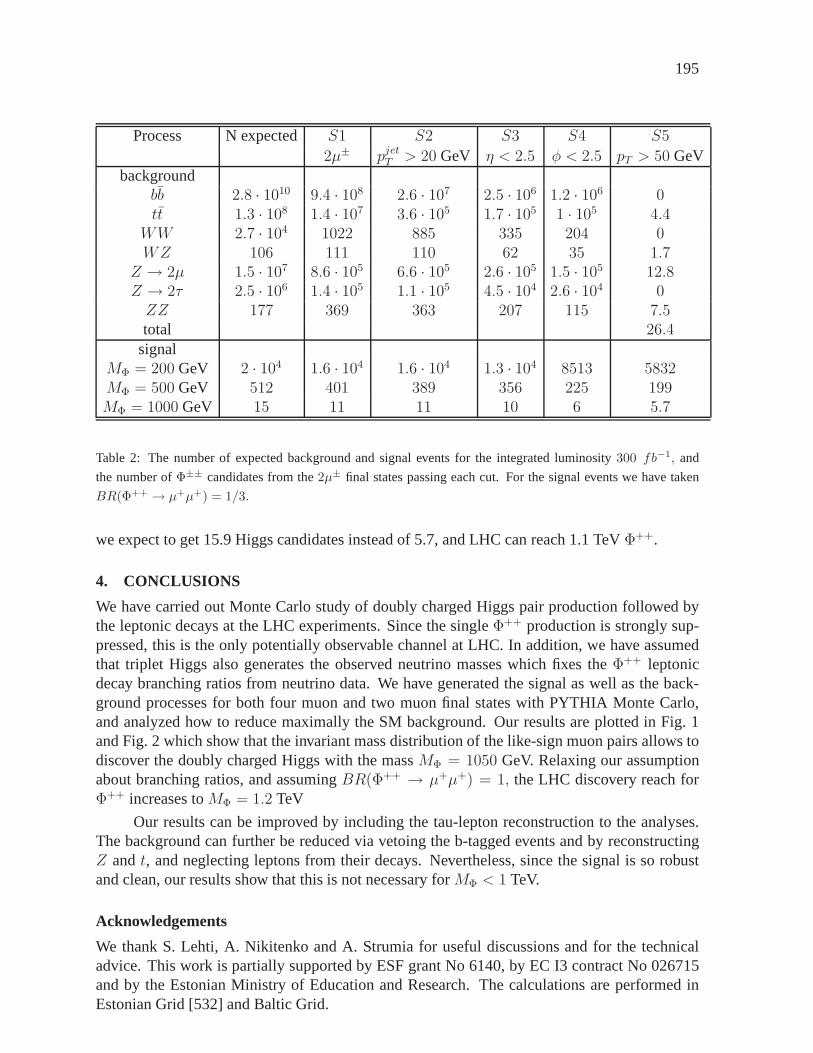
195

Process N expected S1 S2 S3 S4 S5

2µ± pjetT > 20 GeV η < 2.5 φ < 2.5 pT > 50 GeVbackground

bb 2.8 · 1010 9.4 · 108 2.6 · 107 2.5 · 106 1.2 · 106 0tt 1.3 · 108 1.4 · 107 3.6 · 105 1.7 · 105 1 · 105 4.4

WW 2.7 · 104 1022 885 335 204 0WZ 106 111 110 62 35 1.7

Z → 2µ 1.5 · 107 8.6 · 105 6.6 · 105 2.6 · 105 1.5 · 105 12.8Z → 2τ 2.5 · 106 1.4 · 105 1.1 · 105 4.5 · 104 2.6 · 104 0ZZ 177 369 363 207 115 7.5total 26.4

signalMΦ = 200 GeV 2 · 104 1.6 · 104 1.6 · 104 1.3 · 104 8513 5832MΦ = 500 GeV 512 401 389 356 225 199MΦ = 1000 GeV 15 11 11 10 6 5.7

Table 2: The number of expected background and signal eventsfor the integrated luminosity300 fb−1, and

the number ofΦ±± candidates from the2µ± final states passing each cut. For the signal events we have taken

BR(Φ++ → µ+µ+) = 1/3.

we expect to get 15.9 Higgs candidates instead of 5.7, and LHCcan reach 1.1 TeVΦ++.

4. CONCLUSIONS

We have carried out Monte Carlo study of doubly charged Higgspair production followed bythe leptonic decays at the LHC experiments. Since the singleΦ++ production is strongly sup-pressed, this is the only potentially observable channel atLHC. In addition, we have assumedthat triplet Higgs also generates the observed neutrino masses which fixes theΦ++ leptonicdecay branching ratios from neutrino data. We have generated the signal as well as the back-ground processes for both four muon and two muon final states with PYTHIA Monte Carlo,and analyzed how to reduce maximally the SM background. Our results are plotted in Fig. 1and Fig. 2 which show that the invariant mass distribution ofthe like-sign muon pairs allows todiscover the doubly charged Higgs with the massMΦ = 1050 GeV. Relaxing our assumptionabout branching ratios, and assumingBR(Φ++ → µ+µ+) = 1, the LHC discovery reach forΦ++ increases toMΦ = 1.2 TeV

Our results can be improved by including the tau-lepton reconstruction to the analyses.The background can further be reduced via vetoing the b-tagged events and by reconstructingZ andt, and neglecting leptons from their decays. Nevertheless, since the signal is so robustand clean, our results show that this is not necessary forMΦ < 1 TeV.

Acknowledgements

We thank S. Lehti, A. Nikitenko and A. Strumia for useful discussions and for the technicaladvice. This work is partially supported by ESF grant No 6140, by EC I3 contract No 026715and by the Estonian Ministry of Education and Research. The calculations are performed inEstonian Grid [532] and Baltic Grid.

196

dilepton invariant mass in GeV0 200 400 600 800 1000 1200

-1N

eve

nts

/100

Gev

at

300

fb

0

10

20

30

40

50

60

70

80

90

dilepton invariant mass in GeV0 200 400 600 800 1000 1200

-1N

eve

nts

/100

Gev

at

300

fb

0

10

20

30

40

50

60

70

80

90 Background

Signal

dilepton invariant mass in GeV0 200 400 600 800 1000 1200

-1N

eve

nts

/100

Gev

at

300

fb

0

2

4

6

8

10

12

14

16

dilepton invariant mass in GeV0 200 400 600 800 1000 1200

-1N

eve

nts

/100

Gev

at

300

fb

0

2

4

6

8

10

12

14

16Background

Signal

Figure 2: Distribution of the invariant mass of two like-sign muons passing all the cuts for the2µ± final state in

the case ofMΦ = 500 GeV (left panel) andMΦ = 1000 GeV (right panel).

197

Part 29

Polarization and spin correlation effects inthird family resonancesG. Azuelos, B. Brelier, D. Choudhury, P.-A. Delsart, R.M. Godbole, S.D. Rindani, R.K. Singhand K. Wagh

AbstractIn this note, we look at using the polarization of third generation fermionsproduced at the LHC in the decay of a high-mass vector resonance toextract information on its couplings. We explore the utility of a fewspin sensitive variables in the case ofτ pair resonances, giving resultsevaluated at parton level. In the case oftt final states, we first presenttheoretically expected single-top polarizations taking the example of theLittlest Higgs model. We then explore a few variables constructed outof the decay lepton variables. We find some sensitivity in spite of thelarge SM background. More detailed simulation studies are in progress.

1. INTRODUCTION

The properties and interactions of quarks and leptons belonging to the third family are stillrelatively poorly measured. The question arises, therefore, if they are just a copy of those ofthe first two families. The universality of interactions is anatural prediction of the Standardmodel (SM), but the number of generations and the relative masses in the model seem com-pletely ad hoc. Serious constraints have been set on the universality of couplings of the firsttwo generations, but for the third, it is less well tested. There are, in fact, reasons to believethat different electroweak and/or strong couplings might apply in this case. For example, al-though the LEP precision measurements are generally in verygood agreement with the SM, theforward-backward asymmetry at theZ pole, in thebb channel is 2.8 standard deviations awayfrom the fitted value [450].

A study of properties of the third generation of fermions is of utmost importance from atheoretical standpoint as well. The Higgs mechanism of Spontaneous Symmetry Breaking is theonly aspect of the Standard Model (SM) which still lacksdirect verification. The large mass ofthe third generation fermions and their consequent large couplings to the Higgs boson motivatea detailed study of their properties and couplings to the gauge bosons and Yukawa couplings tothe Higgs bosons. As a matter of fact, such studies are a focusof all the collider-based inves-tigations which wish to probe/establish the Higgs mechanism. Furthermore, any alternative tothe Higgs mechanism almost certainly involves the top quark[533]. Many theories beyond theSM incorporate a special role for the top quark, because of its high mass,mt ∼ v/

√2, where

v is the vacuum expectation value (vev) of the SM Higgs fields. The well known problem ofthe instability of the Higgs boson mass to radiative corrections is solved in Supersymmetry bycancellation of the divergent contribution due to particleloops by the corresponding contribu-tion from the sparticle loops. To cancel the dominant top quark contribution, without the use ofSupersymmetry, some models, such as the Little Higgs model [458, 534], predict the existenceof an additional heavy isosinglet quark, a heavy top, which could then generally mix with the

198

SM top quark. In Technicolor models, bosons from an extendedgauge group can provide massto the light fermions, but only a fraction of the top mass can thus be explained, and one mustresort to a topcolor assisted Technicolor model (TC2) [535]to understand the observed highmass of the top. For these reasons, it will be important to measure with precision the couplingconstants of this mysterious quark.

The large mass of thet implies that its life time is shorter than the hadronizationtime scaleand thus the decay products maintain the memory of the polarization of the parent (anti)quark.This is normally reflected in the energy and the angular distribution of the decay lepton as wellas in the correlation between the two leptons [536]. Similarly the polarization of theτ lendsitself to a measurement through the energy distribution of the decay pions even at a hadroniccollider [537–539]. Any anomalous interactions that the third generation fermions may have,if chirality or parity violating, may give rise to net polarization of the produced fermion. In theHiggs sector, the effects are also enhanced due to the large mass of these fermions. The possi-bility of exploiting the polarization of the top to probe newphysics at hadron colliders [540],in the continuumtt pair production [541, 542] as well as single top production [543–545] hasbeen subject of many studies. Studies in the context of the resonanttt production such as inHiggs decay [546] or due to s-channel exchange of a spin-2 KK graviton in the Extra Dimen-sional Models [547] have also been performed. The use of finalstate particle polarization inthe probe of new physics at the LHC is currently gathering momentum as many experimentalstrategies continue being sharpened. In this note, we explore the possibility of using the po-larization of the third family fermions produced in the decay of narrow spin-1 resonances atthe LHC. In general, resonances of electroweak or strong interaction nature, of different spins,are predicted in a variety of models: (i)Z ′ in a Left-Right symmetric model, or in E(6) GrandUnified theory [548], (ii)ZH in the Little Higgs model [458, 534], (iii) Kaluza-Klein states ofa graviton, in models with large extra dimensions [403], (iv) Kaluza-Klein states of theZ andγ in TeV−1-size models of extra dimensions [549] or in (v) Higgsless models [550], (vi)η8, πTin Technicolor models, in particular TC2 models [535], or (vii) axigluons in chiral colour mod-els [551], etc. The Tevatron has looked for such resonances and an intriguing excess of eventsin tt invariant mass distributions is seen [552,553]. If such a resonance is found at future collid-ers, a theoretical interpretation will require a measurement of all its properties. Some obviousobservables are the cross section, the width, the branchingratios to the different fermions, andforward-backward asymmetries in their decays. Here, we examine the resolving power of an-other observable, namely the polarization of the decay products, when such a measurement ispossible, i.e. from resonance decays toτ τ andtt.

The present study is at generator level. It aims to explore the differences between the-oretical models for a future more realistic experimental analysis. The differences shown herewill certainly be considerably attenuated by detector resolutions and efficiencies. In the firstsection we present results of a study of the tau polarizationand the spin correlations in theprocessZ ′ → τ τ with aZ ′ with different assumed couplings. We then discuss the predictionsfor polarization of thet in the decay of the resonance, in a particular model, the Littlest Higgsmodel [498]. Following this, we explore possible observables one could construct in the case ofthe tt pair produced resonantly. More detailed studies with the variables we have constructedand the spin-spin correlations between the decay leptons aswell as thett still remain. So dothe investigations into other representative models of a Vector resonance like an axigluon [551]where the production rates will be higher, still remain to bepursued.

199

2. SPIN CORRELATIONS IN Z ′ → τ τ

To study tau polarization and spin correlations in the processZ ′ → τ τ , the program TAUOLA [554]was modified to include aZ ′ resonance. The changes were very simple: it was sufficient toaddthe case where the parent of aτ was aZ ′ and clone theZ/γ treatment for the calculation ofthe probability of longitudinal polarization combinations of theτ leptons, at the level of theamplitudes, thus ensuring that all interferences are takeninto account.

We have evaluated the following spin sensitive observables, as suggested in [555], for thecase, expected to be the most sensitive, ofτ → πν (more generally, to include leptonic decayor three-prong decays, one can replace theπ by the system of charged particles from the decayof theτ ):

1. theπ energy spectrum, relative to theτ energy, in the laboratory frame:z± = pπ±/Eτ ,2. the distribution of number of events as a function of theπ+π− Energy-Energy correlation

variablezs. After evaluatinga = zmeasured+ − zmeasured

− , this variablezs is defined as thesigned part of the surface area in the 2-parameter phase spacez+, z− between linesz+= z− andz+ = z− + a (the sign of thea should be taken).

3. theπ+π− invariant mass.

In order to evaluate the sensitivity to couplings, a vector resonance,Z ′, of mass 1 TeV, wasconsidered under different coupling scenarios: (i) Standard Model-like couplings, (ii)sin2 θW =0 (which could find some justification [556] in the Higgsless model) and (iii) a right-handedZ ′, as well as (iv) a case with noτ polarization. Effects of initial or final state radiation areincluded, but it must be stressed that no detector effects are applied, except for a lowerpT cutof 30 GeV and a pseudo-rapidity cut of|η| < 2.5 on the emittedπ’s. The distributions obtainedrepresent, therefore, parton-level distributions, wherereconstruction efficiencies or resolutionshave not been taken into account. The reconstruction of aτ -pair resonance is possible at theLHC, in spite of the presence of neutrinos in the final state. Neglecting the mass of theτ leptonsand making the approximation that the neutrino transverse momenta are in the same directionas theτ itself: with the measurement ofpmissT and momentum vectors of the charged decayproducts, there are enough constraints to reconstruct fully the kinematics [557]. The method,however, has a singularity when the twoτ ’s are exactly back to back, which occurs when theresonance is very heavy, and essentially produced at rest. It must be expected, therefore, thatthe sensitivities obtained above at parton level will be considerably degraded when applied atdetector reconstruction level. This will be the subject of afuture study.

Fig. 1(a) shows the shape of the resonance in the different scenarios,together with theDrell-Yan continuum (Z/γ s-channel contribution and interferences) whereas Fig. 1(b) showsthe slope of thez− distribution as a function of the invariant mass of the twoτ ’s. The interfer-ence region of the Drell-Yan andZ ′ resonance is particularly sensitive to its couplings.

It is interesting to compare the distribution of the normalizedππ invariant mass in thepresence of theZ ′ with that for the SM Drell-Yan tail, in the interference region. As can beseen the shape of theππ invariant mass distribution, shown in Fig. 2 is not much altered bythe presence of aZ ′ resonance with SM couplings, but changes very significantlyfor the othercases studied, with different couplings.

Fig. 3(a) shows the sensitivity to the couplings of the Forward-Backward asymmetry inthe decay of theZ ′, defined as

AFB =N+ −N−N+ +N−

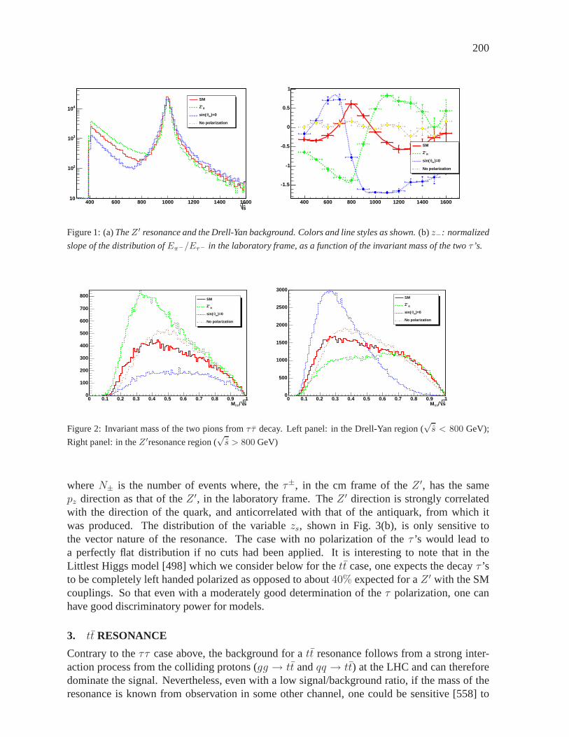
200

s400 600 800 1000 1200 1400 1600

10

210

310

410

SM

RZ’

)=0wθsin(

No polarization

400 600 800 1000 1200 1400 1600

-1.5

-1

-0.5

0

0.5

1

SM

RZ’

)=0wθsin(

No polarization

Figure 1: (a)TheZ ′ resonance and the Drell-Yan background. Colors and line styles as shown.(b) z−: normalized

slope of the distribution ofEπ−/Eτ− in the laboratory frame, as a function of the invariant mass of the twoτ ’s.

s/ππM0 0.1 0.2 0.3 0.4 0.5 0.6 0.7 0.8 0.9 1

0

100

200

300

400

500

600

700

800SM

RZ’

)=0wθsin(

No polarization

s/ππM0 0.1 0.2 0.3 0.4 0.5 0.6 0.7 0.8 0.9 1

0

500

1000

1500

2000

2500

3000SM

RZ’

)=0wθsin(

No polarization

Figure 2: Invariant mass of the two pions fromτ τ decay. Left panel: in the Drell-Yan region (√s < 800 GeV);

Right panel: in theZ ′resonance region (√s > 800 GeV)

whereN± is the number of events where, theτ±, in the cm frame of theZ ′, has the samepz direction as that of theZ ′, in the laboratory frame. TheZ ′ direction is strongly correlatedwith the direction of the quark, and anticorrelated with that of the antiquark, from which itwas produced. The distribution of the variablezs, shown in Fig. 3(b), is only sensitive tothe vector nature of the resonance. The case with no polarization of the τ ’s would lead toa perfectly flat distribution if no cuts had been applied. It is interesting to note that in theLittlest Higgs model [498] which we consider below for thett case, one expects the decayτ ’sto be completely left handed polarized as opposed to about40% expected for aZ ′ with the SMcouplings. So that even with a moderately good determination of theτ polarization, one canhave good discriminatory power for models.

3. tt RESONANCE

Contrary to theττ case above, the background for att resonance follows from a strong inter-action process from the colliding protons (gg → tt andqq → tt) at the LHC and can thereforedominate the signal. Nevertheless, even with a low signal/background ratio, if the mass of theresonance is known from observation in some other channel, one could be sensitive [558] to

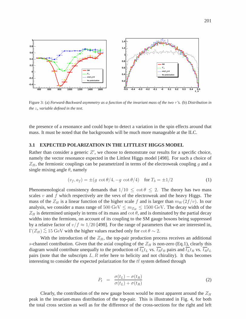
201

400 600 800 1000 1200 1400 1600

-0.4

-0.2

0

0.2

0.4

0.6

0.8

1

SM

RZ’

)=0wθsin(

No polarization

z_s-0.5 -0.4 -0.3 -0.2 -0.1 -0 0.1 0.2 0.3 0.4 0.50

0.2

0.4

0.6

0.8

1

1.2

1.4

SM

RZ’

)=0wθsin(

No polarization

Figure 3: (a)Forward-Backward asymmetry as a function of the invariant mass of the twoτ ’s. (b) Distribution in

thezs variable defined in the text.

the presence of a resonance and could hope to detect a variation in the spin effects around thatmass. It must be noted that the backgrounds will be much more manageable at the ILC.

3.1 EXPECTED POLARIZATION IN THE LITTLEST HIGGS MODEL

Rather than consider a genericZ ′, we choose to demonstrate our results for a specific choice,namely the vector resonance expected in the Littlest Higgs model [498]. For such a choice ofZH , the fermionic couplings can be parametrized in terms of theelectroweak couplingg and asingle mixing angleθ, namely

(vf , af) = ±(g cot θ/4,−g cot θ/4) for T3 = ±1/2 (1)

Phenomenological consistency demands that1/10 ≤ cot θ ≤ 2. The theory has two massscalesv andf which respectively are the vevs of the electroweak and the heavy Higgs. Themass of theZH is a linear function of the higher scalef and is larger thanmW (2f/v). In ouranalysis, we consider a mass range of500 GeV ≤ mZH

≤ 1500 GeV. The decay width of theZH is determined uniquely in terms of its mass andcot θ, and is dominated by the partial decaywidths into the fermions, on account of its coupling to the SMgauge bosons being suppressedby a relative factor ofv/f ≈ 1/20 [498]. For the range of parameters that we are interested in,Γ(ZH) <∼ 15 GeV with the higher values reached only forcot θ ∼ 2.

With the introduction of theZH , the top-pair production process receives an additionals-channel contribution. Given that the axial coupling of theZH is non-zero (Eq.1), clearly thisdiagram would contribute unequally to the production oftLtL vs. tRtR pairs andtLtR vs. tRtLpairs (note that the subscriptsL,R refer here to helicity and not chirality). It thus becomesinteresting to consider the expected polarization for thett system defined through

Pt =σ(tL) − σ(tR)

σ(tL) + σ(tR)(2)

Clearly, the contribution of the new gauge boson would be most apparent around theZHpeak in the invariant-mass distribution of the top-pair. This is illustrated in Fig. 4, for boththe total cross section as well as for the difference of the cross-sections for the right and left

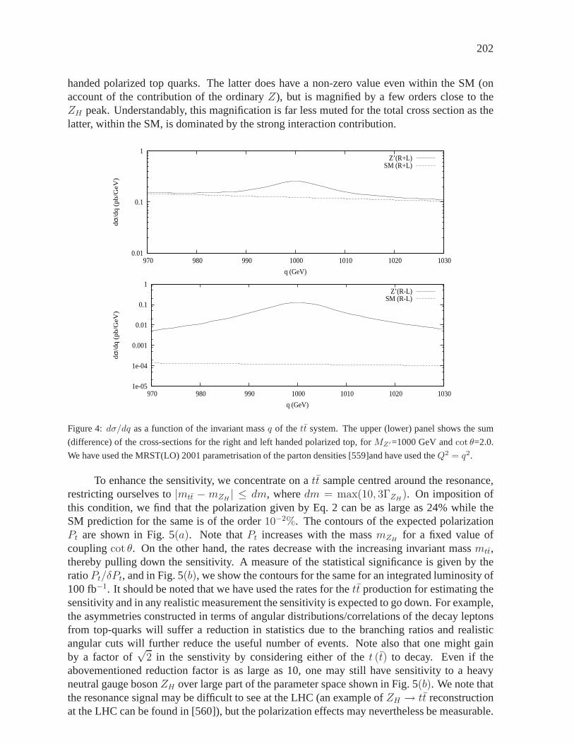
202

handed polarized top quarks. The latter does have a non-zerovalue even within the SM (onaccount of the contribution of the ordinaryZ), but is magnified by a few orders close to theZH peak. Understandably, this magnification is far less muted for the total cross section as thelatter, within the SM, is dominated by the strong interaction contribution.

0.01

0.1

1

970 980 990 1000 1010 1020 1030

dσ/d

q (

pb

/Ge

V)

q (GeV)

Z’(R+L)SM (R+L)

1e-05

1e-04

0.001

0.01

0.1

1

970 980 990 1000 1010 1020 1030

dσ/d

q (

pb

/Ge

V)

q (GeV)

Z’(R-L)SM (R-L)

Figure 4:dσ/dq as a function of the invariant massq of the tt system. The upper (lower) panel shows the sum

(difference) of the cross-sections for the right and left handed polarized top, forMZ′=1000 GeV andcot θ=2.0.

We have used the MRST(LO) 2001 parametrisation of the partondensities [559]and have used theQ2 = q2.

To enhance the sensitivity, we concentrate on att sample centred around the resonance,restricting ourselves to|mtt − mZH

| ≤ dm, wheredm = max(10, 3ΓZH). On imposition of

this condition, we find that the polarization given by Eq. 2 can be as large as 24% while theSM prediction for the same is of the order10−2%. The contours of the expected polarizationPt are shown in Fig. 5(a). Note thatPt increases with the massmZH

for a fixed value ofcouplingcot θ. On the other hand, the rates decrease with the increasing invariant massmtt,thereby pulling down the sensitivity. A measure of the statistical significance is given by theratioPt/δPt, and in Fig. 5(b), we show the contours for the same for an integrated luminosity of100 fb−1. It should be noted that we have used the rates for thett production for estimating thesensitivity and in any realistic measurement the sensitivity is expected to go down. For example,the asymmetries constructed in terms of angular distributions/correlations of the decay leptonsfrom top-quarks will suffer a reduction in statistics due tothe branching ratios and realisticangular cuts will further reduce the useful number of events. Note also that one might gainby a factor of

√2 in the senstivity by considering either of thet (t) to decay. Even if the

abovementioned reduction factor is as large as 10, one may still have sensitivity to a heavyneutral gauge bosonZH over large part of the parameter space shown in Fig. 5(b). We note thatthe resonance signal may be difficult to see at the LHC (an example ofZH → tt reconstructionat the LHC can be found in [560]), but the polarization effects may nevertheless be measurable.

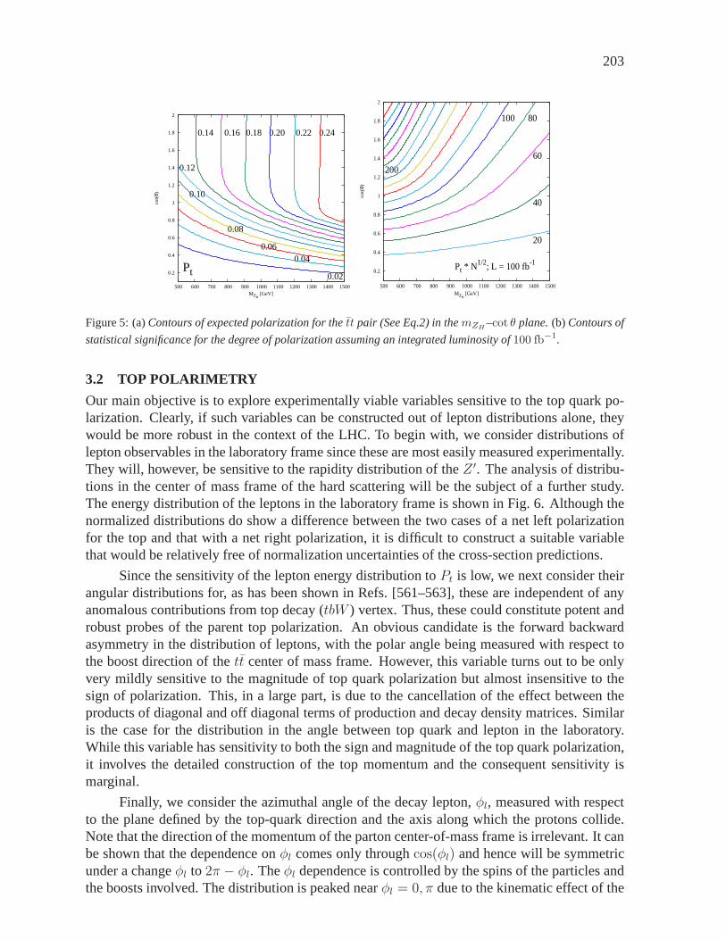
203

0.2

0.4

0.6

0.8

1

1.2

1.4

1.6

1.8

2

500 600 700 800 900 1000 1100 1200 1300 1400 1500

cot(θ

)

MZH [GeV]

0.240.220.200.180.160.14

0.12

0.02

0.040.06

0.08

0.10

Pt 0.2

0.4

0.6

0.8

1

1.2

1.4

1.6

1.8

2

500 600 700 800 900 1000 1100 1200 1300 1400 1500

cot(θ

)

MZH [GeV]

Pt * N1/2; L = 100 fb-1

20

40

60

80100

200

Figure 5: (a)Contours of expected polarization for thett pair (See Eq.2) in themZH–cot θ plane.(b) Contours of

statistical significance for the degree of polarization assuming an integrated luminosity of100 fb−1.

3.2 TOP POLARIMETRY

Our main objective is to explore experimentally viable variables sensitive to the top quark po-larization. Clearly, if such variables can be constructed out of lepton distributions alone, theywould be more robust in the context of the LHC. To begin with, we consider distributions oflepton observables in the laboratory frame since these are most easily measured experimentally.They will, however, be sensitive to the rapidity distribution of theZ ′. The analysis of distribu-tions in the center of mass frame of the hard scattering will be the subject of a further study.The energy distribution of the leptons in the laboratory frame is shown in Fig. 6. Although thenormalized distributions do show a difference between the two cases of a net left polarizationfor the top and that with a net right polarization, it is difficult to construct a suitable variablethat would be relatively free of normalization uncertainties of the cross-section predictions.

Since the sensitivity of the lepton energy distribution toPt is low, we next consider theirangular distributions for, as has been shown in Refs. [561–563], these are independent of anyanomalous contributions from top decay (tbW ) vertex. Thus, these could constitute potent androbust probes of the parent top polarization. An obvious candidate is the forward backwardasymmetry in the distribution of leptons, with the polar angle being measured with respect tothe boost direction of thett center of mass frame. However, this variable turns out to be onlyvery mildly sensitive to the magnitude of top quark polarization but almost insensitive to thesign of polarization. This, in a large part, is due to the cancellation of the effect between theproducts of diagonal and off diagonal terms of production and decay density matrices. Similaris the case for the distribution in the angle between top quark and lepton in the laboratory.While this variable has sensitivity to both the sign and magnitude of the top quark polarization,it involves the detailed construction of the top momentum and the consequent sensitivity ismarginal.

Finally, we consider the azimuthal angle of the decay lepton, φl, measured with respectto the plane defined by the top-quark direction and the axis along which the protons collide.Note that the direction of the momentum of the parton center-of-mass frame is irrelevant. It canbe shown that the dependence onφl comes only throughcos(φl) and hence will be symmetricunder a changeφl to 2π − φl. Theφl dependence is controlled by the spins of the particles andthe boosts involved. The distribution is peaked nearφl = 0, π due to the kinematic effect of the

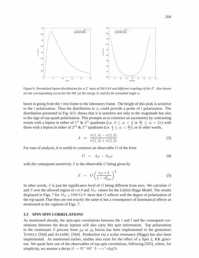
204

0

0.005

0.01

0.015

0.02

0.025

0.03

0.035

0.04

0 50 100 150 200 250

(1/σ

) dσ

/dE

l

El (GeV)

SMZp (left handed coupling)

Zp (right handed coupling)

0.005

0.01

0.015

0.02

0.025

0.03

0.035

0.04

0.045

0.05

0 50 100 150 200 250 300 350 400

(1/σ

) dσ

/dφ

l

φl (Degrees)

SMZp (left handed coupling)

Zp (right handed coupling)

Figure 6:Normalized lepton distributions for aZ ′ mass of 500 GeV and different couplings of theZ ′. Also shown

are the corresponding curves for the SM.(a) the energyEl and(b) the azimuthal angleφl.

boost in going from thet rest frame to the laboratory frame. The height of this peak issensitiveto thet polarization. Thus the distribution inφl could provide a probe oft polarization. Thedistribution presented in Fig. 6(b) shows that it is sensitive not only to the magnitude but alsoto the sign of top-quark polarization. This prompts us to construct an asymmetry by contrastingevents with a lepton in either of1st & 4th quadrants (i.e.0 ≤ φl <

π2

or 3π2

≤ φl < 2π) withthose with a lepton in either of2nd & 3rd quadrants (i.e.π

2≤ φl <

3π2

), or in other words,

A ≡ σ(1, 4) − σ(2, 3)

σ(1, 4) + σ(2, 3)(3)

For ease of analysis, it is useful to construct an observableO of the form

O = AZ′ − ASM (4)

with the consequent sensitivityS to the observableO being given by

S = O

(σZ′ ∗ L

1 −A2SM

) 1

2

(5)

In other words,S is just the significance level ofO being different from zero. We calculateOandS over the allowed region ofcot θ andMZ′ values for theLittlest Higgs Model. The resultsdisplayed in Figs. 7 forMZ′ ¡ 1000 GeV show thatO reflects well the degree of polarization ofthe top-quark That they are not exactly the same is but a consequence of kinematical effects asmentioned in the captions of Figs. 7.

3.3 SPIN SPIN CORRELATIONS

As mentioned already, the spin-spin correlations between the t and t and the consequent cor-relations between the decay leptons will also carry this spin information. Top polarizationin the continuumtt process fromgg or qq fusion has been implemented in the generatorsTOPREX [564] and ACERMC [564]. Production via a scalar resonance (Higgs) has also beenimplemented. As mentioned earlier, studies also exist for the effect of a Spin 2, KK gravi-ton. We quote here one of the observables of top spin correlations, following [565], where, forsimplicity, we assume a decaytt→W+bW−b→ e+νbqq′b:

205

0.2

0.4

0.6

0.8

1

1.2

1.4

1.6

1.8

2

500 550 600 650 700 750 800 850 900 950 1000

co

t(θ)

MZH [GeV]

0.025 0.020 0.015 0.012 0.010 0.008 0.006 0.004

0.002

0.001

O

Figure 7: (a)The observableO as a function ofcot θ andMZ′ . As can be seen from Fig. 5, for constantMZ′

the observable follows the same trends as the top-quark polarization. However, there are some kinematical effects

which lead to different trends for constant couplings and varyingMZ′ , as compared to top-quark polarization.(b)

The sensitivityS for the observableO as a function ofcot θ andMZ′ . As can be seen from Fig. 5(b), S follows the

same trends as top-quark polarization sensitivity.

1. the correlation in angular distribution of the two top quarks:

1

N

d2N

d cos θ1 d cos θ2=

1

4(1 +B1 cos θ1 +B2 cos θ2 − C cos θ1 cos θ2) (6)

whereθ1 (θ2) are respectively the angles between the direction of thee+ (e−) in the restframes oft (t,) and the direction of thet (t) in the rest frame of thett system.

2. the distribution of the opening angleΦ between the two leptons

1

N

dN

d cos Φ=

1

2(1 −D cos Φ) (7)

Such studies applied to aZ ′ with arbitrary couplings still need to be implemented.

4. CONCLUSIONS

Resonances involving third generation fermions can revealvaluable information on effects be-yond the Standard Model. Here, studies of polarization and spin correlation observables forheavyτ τ andtt resonances at the LHC have been performed at parton level andother observ-ables have yet to be evaluated. These initial studies show that there is some sensitivity to thecouplings of such resonances. More work needs to be done, however, to evaluate in more real-istic scenarios, involving detector simulation and reconstruction effects, the possibility of usingthese observables in determining the couplings of these resonances to theτ leptons andt quarks.

Acknowledgements

We thank Z. Was for helpful discussions. RG, SDR and RKS wish to acknowledge partialsupport from the IndoFrench Centre for Cooperation in Advanced Research (IFCPAR) underproject number IFC/3004-B/2004.

206

Part 30

Charged Higgs boson studies at theTevatron and LHCV. Bunichev, L. Dudko, S. Hesselbach, S. Moretti, S. Perries, J. Petzoldt, A. Pompos, J. Rathsmanand A. Sopczak

AbstractWe report on detailed Monte Carlo comparison of selection variablesused to separatetbH± signal events from the Standard Modeltt back-ground. While kinematic differences exist between the two processeswhenevermH± 6= mW , in the particularly challenging case of the neardegeneracy of the charged Higgs boson mass with theW mass, the ex-ploration of the spin difference between the charged Higgs and theWgauge boson becomes crucial. The latest implementation of the chargedHiggs boson process into PYTHIA is used to generate the signal events.The TAUOLA package is used to decay the tau lepton emerging fromthe charged Higgs boson decay. The spin information is then transferredto the final state particles. Distributions of selection variables are foundto be very similar for signal and background, rendering the degeneratemass region particularly challenging for aH± discovery, though somescope exists at both colliders. In addition, the change in the behavior ofkinematic variables from Tevatron to LHC energies is brieflydiscussed.

1. INTRODUCTION

The importance of charged Higgs boson searches at future colliders has in the recent yearsbeen emphasized [177, 566–568] for LEP, a future International Linear Collider (ILC), theTevatron and the Large Hadron Collider (LHC), as the detection of the charged Higgs bosonwould be a definite signal for the existence of New Physics going beyond the Standard Model(SM) [569, 570]. The charged Higgs boson states are naturally accommodated in non-minimalHiggs scenarios, like the Two-Higgs Doublet Models (2HDMs). A Supersymmetric version ofthe latter is the Minimal Supersymmetric Standard Model (MSSM). It is a Type II 2HDM withspecific relations among neutral and charged Higgs boson masses and couplings, dictated bySupersymmetry (SUSY) [571].

The Tevatron collider at Fermilab is currently in its secondstage of operation, so-calledRun 2, with a higher center-of-mass (CM) energy of

√s = 1.96 TeV. This machine will be

the first one to probe charged Higgs boson masses in the mass range up tomH± ∼ mt [568].Starting from 2008, the LHC at CERN will be in a position to confirm or rule out the existenceof such a particle over a very large portion of both the 2HDM and MSSM parameter space,mH± <∼ 400 GeV, depending ontan β (see the reviews [572–574]).

At present, a lower bound on the charged Higgs boson mass exists from LEP [575],mH± <∼ mW , independently of the charged Higgs boson decay Branching Ratios (BRs). Thislimit is valid within any Type II 2HDM whereas, in the lowtanβ region (below about 3), an

207

indirect lower limit onmH± can be derived in the MSSM from the one onmA (the mass of thepseudoscalar Higgs state of the model):m2

H± ≈ m2W +m2

A>∼ (130 GeV)2.

If the charged Higgs boson massmH± satisfiesmH± < mt−mb, wheremt is the top quarkmass andmb the bottom quark mass,H± particles could be produced in the decay of on-shell(i.e.,Γt → 0) top (anti-)quarkst→ bH+, the latter being in turn produced in pairs viagg fusionandqq annihilation. This approximation was the one customarily used in event generators whenmH± <∼ mt. Throughout this paper we adopt the same notation as in Ref. [576]: charged Higgsproduction is denoted byqq, gg → tt → tbH± if due to (anti-)top decays and byqq, gg →tbH± if further production diagrams are included. Owing to the large top decay width (Γt ≃1.5 GeV) and due to the additional diagrams which do not proceed via directtt production [577–579], charged Higgs bosons could also be produced at and beyond the kinematic top decaythreshold. The importance of these effects in the so-called‘threshold’ or ‘transition’ region(mH± ≈ mt) was emphasized in previous Les Houches proceedings [580, 581] as well as inRefs. [576,582–584] and the calculations of Refs. [577,578] (based on the appropriateqq, gg →tbH± description) are now implemented in HERWIG [11–13, 585] andPYTHIA [16, 17, 46,586, 587]. (A comparison between the two generators was carried out in Ref. [576].) For anyrealistic simulation ofH± production withmH± >∼ mt the use of these implementations is ofparamount importance. In addition, in the mass region near the top quark mass, a matching ofthe calculations for theqq, gg → tbH± andgb→ tH± processes might be required [587].

A charged Higgs boson withmH± <∼ mt decays predominantly into aτ lepton and aneutrino. For large values oftan β ( >∼ 5), the ratio of the vacuum expectation values of the twoHiggs doublets, the corresponding branching ratio is near 100%. FormH± >∼ mt, H± → τνis overwhelmed byH± → tb, but the latter is much harder to disentangle from backgroundthan the former. The associated top quark decays predominantly into aW boson, or at times asecond charged Higgs boson, and ab quark. The reaction

qq, gg → tbH± (t→ bW ) (H± → τ±ντ ) (1)

is then a promising channel to search for the charged Higgs boson at both the Tevatron (wherethe dominant production mode isqq) and the LHC (wheregg is the leading subprocess). If theH± → τν decay channel is used to search for Higgs bosons, then a key ingredient in the signalselection process should be the exploration of decay distributions that are sensitive to the spinnature of the particle yielding theτ lepton (H± orW±), as advocated in Refs. [538, 588–590](see also [591,592]).

It is the purpose of this contribution to outline the possible improvements that can beachieved at the Tevatron and LHC in the search for charged Higgs bosons, with mass below,near or abovemt, when both the appropriate description of the Higgs production process andpolarization effects are used to sharpen theH± → τν signature.

2. EXPERIMENTAL SIMULATION AT THE TEVATRON ENERGY

We start by studying charged Higgs productionqq, gg → tbH± with subsequent decayst →bW , H± → τ±ντ at the FNAL Tevatron with

√s = 1.96 TeV. In the following we analyse

hadronic decays of theW boson andτ lepton (W → qq′, τ → hadrons + ντ ), which results inthe signature2b+2j+τjet+ 6Pt (2 b jets, 2 light jets, 1τ jet and missing transverse momentum).The most important background process isqq, gg → tt with the subsequent decayst → bW+

and t → bW−, oneW boson decaying hadronically (W → qq′) and one leptonically (W →τντ ), which results in the same final state particles as for the expected signal.

208

The signal processqq, gg → tbH± is simulated with PYTHIA [16, 17, 46, 586] usingthe implementation described in [587], in order to take the effects in the transition region intoaccount. The subsequent decayst → bW , W → qq′ andH± → τ±ντ are carried out withinPYTHIA, whereas the tau leptons are decayed externally withthe program TAUOLA [554,593],which includes the complete spin structure of theτ decay. The background processqq, gg → ttis also simulated with PYTHIA with the built-in subroutinesfor tt production. Here, the decaysof the top quarks andW bosons are performed within PYTHIA and that of theτ lepton withinTAUOLA.

The momentum of the finalb and light quarks from the PYTHIA event record is taken asthe momentum of the corresponding jet, whereas for theτ jet the sum of all non-leptonic finalstate particles as given by TAUOLA is used. The energy resolution of the detector is emulatedthrough a Gaussian smearing(∆(Pt)/Pt)

2 = (0.80/√Pt)

2 of the transverse momentumPt forall jets in the final state, including theτ jet [568]. Theτ -spin information affects both the energyand the angular distribution of theτ decay products. As a basic cut the transverse momenta ofthese final jets are required to be larger than5 GeV. The missing transverse momentum6Ptis constructed from the transverse momenta of all visible jets (including the visibleτ decayproducts).

The signal and background processes have been simulated fortanβ = 30 andmH± =80, 100 and160 GeV with PYTHIA, version 6.325. As shown in [576], the signalcross sectiontbH± agrees with the one from the top-decay approximationtt→ tbH± for charged Higgs bo-son masses up to about 160 GeV. For this to be true the same factorization and renormalizationscales have to be used, as well as the same scale for the running b quark mass. In this studywe have used the factorization scale(mt +mH±)/4 [587], the renormalization scalemH± , andthe runningb quark mass has been evaluated atmH± for both the signal and the background forconsistency. This results in a dependence of the backgroundcalculations ontan β andmH± .However, the cross sections have then been rescaled with a common factor such that the totalttcross section isσprod

tt = 5220 fb [594]. The resulting cross sections into the final state with thesignature2b+2j+τjet+ 6Pt for signal and background are given in Table 1 before (σth) and after(σ) applying the basic cutP jet

t > 5 GeV. For the three signal masses, thetbH± andtt→ tbH±

cross section calculations agree numerically. The cross sectionσth for the background is givenby

σth = σprodtt 2BR(t→ bW+)2BR(W → jj)BR(W → τν)BR(τ → ν + hadrons), (2)

whereas the signal is given by

σth = σprodtbH±BR(t→ bW+)BR(W → jj)BR(H+ → τν)BR(τ → ν + hadrons), (3)

or alternatively, in the top-decay approximation, by

σth = σprodtt 2BR(t→ bH+)BR(t→ bW+)BR(W → jj)

BR(H+ → τν)BR(τ → ν + hadrons). (4)

The kinematic selection variables are shown in Figs. 1–9 fora simulation at the Tevatronenergy of 1.96 TeV and a 80 GeV charged Higgs boson. For this mass the kinematic signaldistributions are very similar to those of the SMtt background. The distributions of signaland background are normalized such that the maximum value inboth distributions coincide, inorder to make small differences better visible. The different spin of the charged Higgs boson

209

Table 1: Tevatron cross sections of backgroundqq, gg → tt and signalqq, gg → tbH± for tanβ = 30 and

mH± = 80, 100 and160 GeV into the final state2b + 2j + τjet+ 6 Pt before (σth) and after (σ) the basic cut of

Pt > 5 GeV for all jets after smearing of the momenta as decribed in the text has been applied.qq, gg → tt qq, gg → tbH±

mH± = 80 GeV mH± = 80 GeV mH± = 100 GeV mH± = 160 GeVσth (fb) 354 538 413 38σ (fb) 312 508 392 34

and theW boson has only a small effect on most of the event variables. Asignificant differencehowever occurs in thePt distribution of theτ jet, so that this variable can be further explored todistinguish between signal and background.

The kinematic selection is based on the method of so-called “Optimal Observables” [581](page 69), which provide the universal procedure to find the complete set of kinematic variablesneeded to separate one physics process from another. Based on this method we can distinguishthree possible classes of variables for the analysis. They are:

• Singular variables. In the case ofmH± = 80 GeV exactly the same ‘singularities’ inphase space are expected for thetbH± signal andtt background. Thus, no variable ofthis class can help to disentangle the former from the latter. For other Higgs mass valuesthe position of the singularities will instead change and wecan use this class of variablesfor the separation of signal and background events.

• Threshold variables. Owing to the same reason of equalH± andW masses, no variablesof this class are useful to distinguish between mass degenerate signal and background,since the energy thresholds are the same in the two processes. FormH± 6= mW , somescope exists.

• Spin variables. In the signal process the spin-0 Higgs particle produces the tau-leptonwhile in the background the tau arises from the decay of the spin-1 W vector boson.We can then expect that some of the variables of this class canhelp us to separate thetwo processes. There are no universal answers on how to choose these variables and eachparticular choice requires a phenomenological study to determine the optimal basis wherethe effects of spin correlations are most significant. On onehand, the scalar Higgs bosonwill decay isotropically and no correlations between production and decay process areexpected. On the other hand, for the background spin correlations between the productionand the decay of aW should be manifest, due to the vectorial nature of the gauge boson.It is precisely the exploration of these correlations that should offer the possibility ofdistinguishing signal from background.

In Figs. 1–9 we can identify distributions of different variables from the first two classes.Here, the signal and background spectra are almost identical for the chosen Higgs boson mass.The next step is to investigate the spin variables. An an example of spin dependent variable wetake thePt distribution of the tau lepton (Fig. 1, Left). Here, differences between theH± andW spectra are visible. Thus, the generated event sample is suitable for further studies of thespin dependent properties of the signal and background reactions considered.

A unique feature of the2b+2j+τjet+ 6Pt signature in particle detectors is the presence ofthe tau lepton. When searching experimentally for the charged Higgs boson signal, not only themagnitude of the production cross section is important, butalso the efficiency of identifying thetau lepton in the hadronic environment plays a crucial role.Since tau leptons have a very short

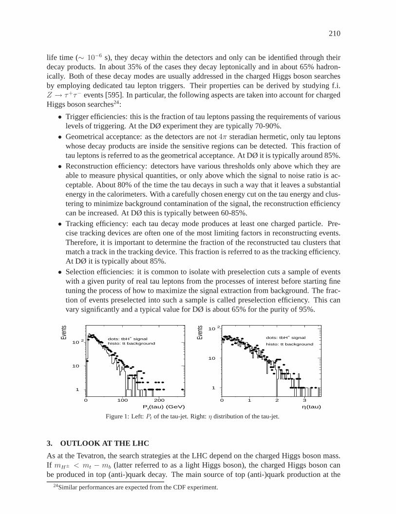
210

life time (∼ 10−6 s), they decay within the detectors and only can be identifiedthrough theirdecay products. In about 35% of the cases they decay leptonically and in about 65% hadron-ically. Both of these decay modes are usually addressed in the charged Higgs boson searchesby employing dedicated tau lepton triggers. Their properties can be derived by studying f.i.Z → τ+τ− events [595]. In particular, the following aspects are taken into account for chargedHiggs boson searches24:

• Trigger efficiencies: this is the fraction of tau leptons passing the requirements of variouslevels of triggering. At the DØ experiment they are typically 70-90%.

• Geometrical acceptance: as the detectors are not4π steradian hermetic, only tau leptonswhose decay products are inside the sensitive regions can bedetected. This fraction oftau leptons is referred to as the geometrical acceptance. AtDØ it is typically around 85%.

• Reconstruction efficiency: detectors have various thresholds only above which they areable to measure physical quantities, or only above which thesignal to noise ratio is ac-ceptable. About 80% of the time the tau decays in such a way that it leaves a substantialenergy in the calorimeters. With a carefully chosen energy cut on the tau energy and clus-tering to minimize background contamination of the signal,the reconstruction efficiencycan be increased. At DØ this is typically between 60-85%.

• Tracking efficiency: each tau decay mode produces at least one charged particle. Pre-cise tracking devices are often one of the most limiting factors in reconstructing events.Therefore, it is important to determine the fraction of the reconstructed tau clusters thatmatch a track in the tracking device. This fraction is referred to as the tracking efficiency.At DØ it is typically about 85%.

• Selection efficiencies: it is common to isolate with preselection cuts a sample of eventswith a given purity of real tau leptons from the processes of interest before starting finetuning the process of how to maximize the signal extraction from background. The frac-tion of events preselected into such a sample is called preselection efficiency. This canvary significantly and a typical value for DØ is about 65% for the purity of 95%.

histo: tt backgrounddots: tbH+ signal

Pt(tau) (GeV)

Even

ts

1

10

10 2

0 100 200

histo: tt background

dots: tbH+ signal

η(tau)

Even

ts

1

10

10 2

0 1 2 3

Figure 1: Left:Pt of the tau-jet. Right:η distribution of the tau-jet.

3. OUTLOOK AT THE LHC

As at the Tevatron, the search strategies at the LHC depend onthe charged Higgs boson mass.If mH± < mt − mb (latter referred to as a light Higgs boson), the charged Higgs boson canbe produced in top (anti-)quark decay. The main source of top(anti-)quark production at the

24Similar performances are expected from the CDF experiment.

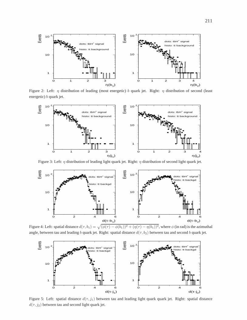
211

histo: tt background

dots: tbH+ signal

η(b1)

Even

ts

1

10

10 2

0 1 2 3

histo: tt background

dots: tbH+ signal

η(b2)

Even

ts

1

10

10 2

0 1 2 3 4

Figure 2: Left: η distribution of leading (most energetic)b quark jet. Right: η distribution of second (least

energetic)b quark jet.

histo: tt background

dots: tbH+ signal

η(j1)

Even

ts

1

10

10 2

0 1 2 3

histo: tt background

dots: tbH+ signal

η(j2)

Even

ts

1

10

10 2

0 1 2 3 4

Figure 3: Left:η distribution of leading light quark jet. Right:η distribution of second light quark jet.

histo: tt backgd

dots: tbH+ signal

d(τ-b1)

Even

ts

1

10

10 2

0 2 4 6

histo: tt backgd

dots: tbH+ signal

d(τ-b2)

Even

ts

1

10

10 2

0 2 4 6

Figure 4: Left: spatial distanced(τ, b1) =√

(φ(τ) − φ(b1))2 + (η(τ) − η(b1))2, whereφ (in rad) is the azimuthal

angle, between tau and leadingb quark jet. Right: spatial distanced(τ, b2) between tau and secondb quark jet.

histo: tt backgddots: tbH+ signal

d(τ-j1)

Even

ts

1

10

10 2

0 2 4 6

histo: tt backgddots: tbH+ signal

d(τ-j2)

Even

ts

1

10

10 2

0 2 4 6

Figure 5: Left: spatial distanced(τ, j1) between tau and leading light quark quark jet. Right: spatial distance

d(τ, j2) between tau and second light quark jet.

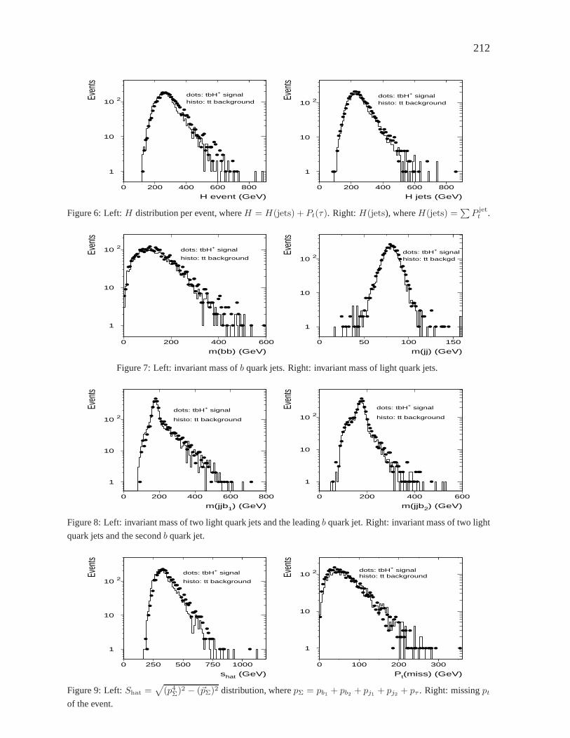
212

histo: tt backgrounddots: tbH+ signal

H event (GeV)

Even

ts

1

10

10 2

0 200 400 600 800

histo: tt backgrounddots: tbH+ signal

H jets (GeV)

Even

ts

1

10

10 2

0 200 400 600 800

Figure 6: Left:H distribution per event, whereH = H(jets) + Pt(τ). Right:H(jets), whereH(jets) =∑P jet

t .

histo: tt background

dots: tbH+ signal

m(bb) (GeV)

Even

ts

1

10

10 2

0 200 400 600

histo: tt backgddots: tbH+ signal

m(jj) (GeV)

Even

ts

1

10

10 2

0 50 100 150

Figure 7: Left: invariant mass ofb quark jets. Right: invariant mass of light quark jets.

histo: tt background

dots: tbH+ signal

m(jjb1) (GeV)

Even

ts

1

10

10 2

0 200 400 600 800

histo: tt background

dots: tbH+ signal

m(jjb2) (GeV)

Even

ts

1

10

10 2

0 200 400 600

Figure 8: Left: invariant mass of two light quark jets and theleadingb quark jet. Right: invariant mass of two light

quark jets and the secondb quark jet.

histo: tt background

dots: tbH+ signal

shat (GeV)

Even

ts

1

10

10 2

0 250 500 750 1000

histo: tt backgrounddots: tbH+ signal

Pt(miss) (GeV)

Even

ts

1

10

10 2

0 100 200 300

Figure 9: Left:Shat =√

(p4Σ)2 − (~pΣ)2 distribution, wherepΣ = pb1 + pb2 + pj1 + pj2 + pτ . Right: missingpt

of the event.

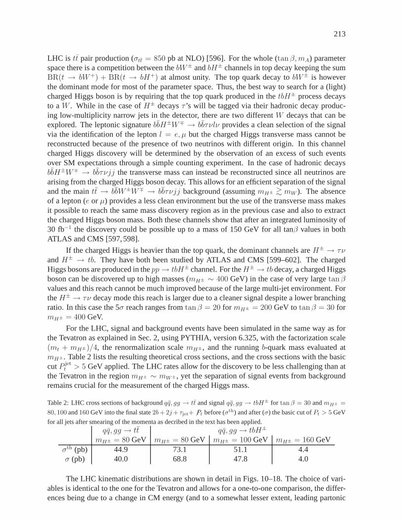
213

LHC is tt pair production (σtt = 850 pb at NLO) [596]. For the whole (tanβ,mA) parameterspace there is a competition between thebW± andbH± channels in top decay keeping the sumBR(t → bW+) + BR(t → bH+) at almost unity. The top quark decay tobW± is howeverthe dominant mode for most of the parameter space. Thus, the best way to search for a (light)charged Higgs boson is by requiring that the top quark produced in thetbH± process decaysto aW . While in the case ofH± decaysτ ’s will be tagged via their hadronic decay produc-ing low-multiplicity narrow jets in the detector, there aretwo differentW decays that can beexplored. The leptonic signaturebbH±W∓ → bbτνlν provides a clean selection of the signalvia the identification of the leptonl = e, µ but the charged Higgs transverse mass cannot bereconstructed because of the presence of two neutrinos withdifferent origin. In this channelcharged Higgs discovery will be determined by the observation of an excess of such eventsover SM expectations through a simple counting experiment.In the case of hadronic decaysbbH±W∓ → bbτνjj the transverse mass can instead be reconstructed since all neutrinos arearising from the charged Higgs boson decay. This allows for an efficient separation of the signaland the maintt → bbW±W∓ → bbτνjj background (assumingmH± >∼ mW ). The absenceof a lepton (e or µ) provides a less clean environment but the use of the transverse mass makesit possible to reach the same mass discovery region as in the previous case and also to extractthe charged Higgs boson mass. Both these channels show that after an integrated luminosity of30 fb−1 the discovery could be possible up to a mass of 150 GeV for all tanβ values in bothATLAS and CMS [597,598].

If the charged Higgs is heavier than the top quark, the dominant channels areH± → τνandH± → tb. They have both been studied by ATLAS and CMS [599–602]. The chargedHiggs bosons are produced in thepp→ tbH± channel. For theH± → tb decay, a charged Higgsboson can be discovered up to high masses (mH± ∼ 400 GeV) in the case of very largetan βvalues and this reach cannot be much improved because of the large multi-jet environment. FortheH± → τν decay mode this reach is larger due to a cleaner signal despite a lower branchingratio. In this case the 5σ reach ranges fromtanβ = 20 for mH± = 200 GeV totan β = 30 formH± = 400 GeV.

For the LHC, signal and background events have been simulated in the same way as forthe Tevatron as explained in Sec. 2, using PYTHIA, version 6.325, with the factorization scale(mt + mH±)/4, the renormalization scalemH±, and the runningb-quark mass evaluated atmH± . Table 2 lists the resulting theoretical cross sections, and the cross sections with the basiccutP jet

t > 5 GeV applied. The LHC rates allow for the discovery to be less challenging than atthe Tevatron in the regionmH± ∼ mW±, yet the separation of signal events from backgroundremains crucial for the measurement of the charged Higgs mass.

Table 2: LHC cross sections of backgroundqq, gg → tt and signalqq, gg → tbH± for tanβ = 30 andmH± =

80, 100 and160 GeV into the final state2b+ 2j+ τjet+ 6Pt before (σth) and after (σ) the basic cut ofPt > 5 GeV

for all jets after smearing of the momenta as decribed in the text has been applied.qq, gg → tt qq, gg → tbH±

mH± = 80 GeV mH± = 80 GeV mH± = 100 GeV mH± = 160 GeVσth (pb) 44.9 73.1 51.1 4.4σ (pb) 40.0 68.8 47.8 4.0

The LHC kinematic distributions are shown in detail in Figs.10–18. The choice of vari-ables is identical to the one for the Tevatron and allows for aone-to-one comparison, the differ-ences being due to a change in CM energy (and to a somewhat lesser extent, leading partonic

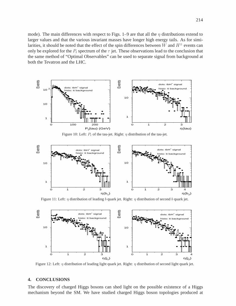
214

mode). The main differences with respect to Figs. 1–9 are that all theη distributions extend tolarger values and that the various invariant masses have longer high energy tails. As for simi-larities, it should be noted that the effect of the spin differences betweenW andH± events canonly be explored for thePt spectrum of theτ jet. These observations lead to the conclusion thatthe same method of “Optimal Observables” can be used to separate signal from background atboth the Tevatron and the LHC.

histo: tt backgrounddots: tbH+ signal

Pt(tau) (GeV)

Even

ts

1

10

10 2

0 100 200

histo: tt background

dots: tbH+ signal

η(tau)

Even

ts1

10

0 1 2 3

Figure 10: Left:Pt of the tau-jet. Right:η distribution of the tau-jet.

histo: tt backgrounddots: tbH+ signal

η(b1)

Even

ts

1

10

0 1 2 3

histo: tt background

dots: tbH+ signal

η(b2)

Even

ts

1

10

0 1 2 3 4

Figure 11: Left:η distribution of leadingb quark jet. Right:η distribution of secondb quark jet.

histo: tt background

dots: tbH+ signal

η(j1)

Even

ts

1

10

0 1 2 3

histo: tt background

dots: tbH+ signal

η(j2)

Even

ts

1

10

0 1 2 3 4

Figure 12: Left:η distribution of leading light quark jet. Right:η distribution of second light quark jet.

4. CONCLUSIONS

The discovery of charged Higgs bosons can shed light on the possible existence of a Higgsmechanism beyond the SM. We have studied charged Higgs bosontopologies produced at

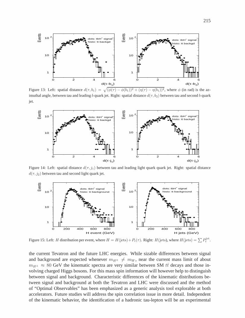
215

histo: tt backgddots: tbH+ signal

d(τ-b1)

Even

ts

1

10

10 2

0 2 4 6

histo: tt backgd

dots: tbH+ signal

d(τ-b2)

Even

ts

1

10

10 2

0 2 4 6

Figure 13: Left: spatial distanced(τ, b1) =√

(φ(τ) − φ(b1))2 + (η(τ) − η(b1))2, whereφ (in rad) is the az-

imuthal angle, between tau and leadingb quark jet. Right: spatial distanced(τ, b2) between tau and secondb quark

jet.

histo: tt backgddots: tbH+ signal

d(τ-j1)

Even

ts

1

10

10 2

0 2 4 6

histo: tt backgddots: tbH+ signal

d(τ-j2)

Even

ts

1

10

10 2

0 2 4 6

Figure 14: Left: spatial distanced(τ, j1) between tau and leading light quark quark jet. Right: spatial distance

d(τ, j2) between tau and second light quark jet.

histo: tt background

dots: tbH+ signal

H event (GeV)

Even

ts

1

10

10 2

0 200 400 600 800

histo: tt background

dots: tbH+ signal

H jets (GeV)

Even

ts

1

10

10 2

0 200 400 600 800

Figure 15: Left:H distribution per event, whereH = H(jets)+Pt(τ). Right:H(jets), whereH(jets) =∑P jet

t .

the current Tevatron and the future LHC energies. While sizable differences between signaland background are expected whenevermH± 6= mW , near the current mass limit of aboutmH± ≈ 80 GeV the kinematic spectra are very similar between SMtt decays and those in-volving charged Higgs bosons. For this mass spin information will however help to distinguishbetween signal and background. Characteristic differences of the kinematic distributions be-tween signal and background at both the Tevatron and LHC werediscussed and the methodof “Optimal Observables” has been emphasized as a generic analysis tool explorable at bothaccelerators. Future studies will address the spin correlation issue in more detail. Independentof the kinematic behavior, the identification of a hadronic tau-lepton will be an experimental

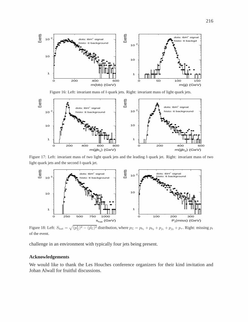
216

histo: tt background

dots: tbH+ signal

m(bb) (GeV)

Even

ts

1

10

10 2

0 200 400 600

histo: tt backgd

dots: tbH+ signal

m(jj) (GeV)

Even

ts

1

10

10 2

0 50 100 150

Figure 16: Left: invariant mass ofb quark jets. Right: invariant mass of light quark jets.

histo: tt background

dots: tbH+ signal

m(jjb1) (GeV)

Even

ts

1

10

10 2

0 200 400 600 800

histo: tt background

dots: tbH+ signal

m(jjb2) (GeV)

Even

ts

1

10

10 2

0 200 400 600

Figure 17: Left: invariant mass of two light quark jets and the leadingb quark jet. Right: invariant mass of two

light quark jets and the secondb quark jet.

histo: tt background

dots: tbH+ signal

shat (GeV)

Even

ts

1

10

10 2

0 250 500 750 1000

histo: tt backgrounddots: tbH+ signal

Pt(miss) (GeV)

Even

ts

1

10

10 2

0 100 200 300

Figure 18: Left:Shat =√

(p4Σ)2 − (~pΣ)2 distribution, wherepΣ = pb1 + pb2 + pj1 + pj2 + pτ . Right: missingpt

of the event.

challenge in an environment with typically four jets being present.

Acknowledgements

We would like to thank the Les Houches conference organizersfor their kind invitation andJohan Alwall for fruitful discussions.

217

Part 31

Diphoton production at the LHC in the RSmodelS. Ferrag, O. Jinnouchi and K. Sridhar

The past decade has been a phase of intense theoretical activity in the area of extra space di-mensions and the resurgence of interest in the physics of extra dimensions is due to the newparadigm of brane-worlds. For high energy physics this new pardigm is exciting because it pro-vides fresh perspectives to the solution of the hierarchy problem and also suggests the discoveryof new physics at TeV-scale colliders.

In an attempt to find a genuine solution to the hierarchy problem Randall and Sundrumdiscovered a model now known in the literature as the Randall-Sundrum model or the RS model25 [470]. In the RS model, one starts with a five-dimensional spacetime where the fifth dimen-sionφ is compactified on aS1/Z2 orbifold with a radiusRc such thatR−1

c is somewhat smallerthanMP , the Planck length. Two D3-branes called the Planck brane and the TeV brane arelocated atφ = 0, π, the orbifold fixed points and the SM fields are localised on the TeV brane.With a five-dimensional metric of the form

ds2 = e−KRcφηµνdxµdxν + R2

cdφ2. (1)

the model provides a novel solution to the hierarchy problem. HereK is a mass scale relatedto the curvature. The warp factor acts as a conformal factor for the fields localised on thebrane and mass factors get rescaled by this factor. SoMP = 1019 GeV for the Planck braneat φ = 0 gets rescaled toMP exp(−KRcπ) for the TeV brane atφ = π. The warp factorgeneratesMP

MEW∼ 1015 by an exponent of order 30 and solves the hierarchy problem. In order

to solve the dynamical problem of stabilisingRc against quantum fluctuations a scalar field inthe bulk [603–606] with a stabilising potential is introduced.

On compactification of the fifth dimension, a tower of massiveKaluza-Klein (KK) exci-tations of the graviton,h(~n)

µν , result on the TeV brane where it interacts with the SM particlesby:

Lint = − 1

MP

T µν(x)h(0)µν (x) − eπKRc

MP

∞∑

1

T µν(x)h(n)µν (x) , (2)

whereMP = MP/√

8π is the reduced Planck mass andT µν is the energy-momentum tensorfor the SM particles. The masses of theh(~n)

µν are given by

Mn = xnK e−πKRc (3)

where thexn are the zeros of the Bessel functionJ1(x) of order unity [605,606]. The resultingmasses of the KK gravitons are not evenly spaced but appear atthe Bessel zeroes. The graviton

25More precisely, these authors proposed two models at more orless the same time with different features ofquantum gravity in each of these. These are now referred to asthe RS1 and RS2 models. In our work, we willdescribe and work with the RS1 model and refer to it throughout as the RS model.

218

zero-mode couples with a1/MP strength and essentially decouples but the couplings of themassive gravitons are enhanced by the exponentialeπKRc leading to interactions of electroweakstrength.

The basic parameters of the RS model are

m0 = Ke−πKRc

c0 = K/MP (4)

wherem0 is a scale of the dimension of mass and sets the scale for the masses of the KKexcitations, andc0 is an effective coupling. It is expected that the parameterc0 lies in the range[0.01, 0.1]. The upper bound onc0 results from requiring thatK is not too large so as to avoidstrong curvature effects and the lower bound ensures thatK is not too small as compared toMP ,since that would introduce a new hierarchy. Values ofm0 are determined in terms ofKRc ∼ 10,so thatm0 ranging from about a 100 GeV to a TeV are possible. Again, avoidance of strongcurvature effects suggests that the mass of the first RS graviton is not too much more than aTeV.

Because of the fact that the zero mode decouples, it is only the heavier modes one canhope to detect in experiments. In the fortuitous circumstance that these modes are within thereach of high-energy experiments, interesting effects like resonance production can be observed,with the resonance decaying within the detectors. If this isnot the case and if the the gravitonsare heavier then the best strategy will be to look for the virtual effects of the gravitons onobservables measured in high-energy collider experiments.

In this paper, we study the virtual effects of the exchange ofspin-2 KK modes, in the RSmodel, in diphoton production at the LHC. The cross-sections for theqq → γγ andgg → γγsubprocesses are [607,608]:

dσ

dt(qq → γγ) =

2πα2Q4q

3s2

1 + cos2θ∗

1 − cos2θ∗(5)

+αQ2

q

96πRe[C(xs)](1 + cos2θ∗) +

s2

24576π|C(xs)|2(1 − cos4θ∗), (6)

and

dσ

dt(gg → γγ) = +

s2

65536π|C(xs)|2(1 + 6cos2θ∗ + cos4θ∗). (7)

The SM box contributiongg → γγ can be neglected because even though at the LHC, this boxcontribution is somewhat increased because of the initial gluon flux but, as shown in Ref. [608],in spite of this increase this contribution is an order of magnitude smaller than the SMqq → γγcontribution for diphoton invariant mass of 500 GeV and is more than two orders of magnitudesmaller for diphoton invariant mass greater than about 1750GeV. On the other hand, the newphysics effects dominate in the large invariant mass bins and, therefore, in the invariant massregion of interest the SM box contribution is negligible even for the case of the LHC.

In the above equations,cosθ∗ is the scattering angle in the partonic c.m. frame,xs ≡√s

m0

andC(x) is defined as

C(x) =32πc20m4

0

λ(x) (8)

219

with

λ(xs) = m20

∑

n

1

s−M2n + iMnΓn

. (9)

and theMn are the masses of the individual resonances and theΓn are the corresponding widths.The graviton widths are obtained by calculating their decays into final states involving SMparticles. This gives

Γn = m0c20x

3n∆n (10)

where

∆n = ∆γγn + ∆gg

n + ∆WWn + ∆ZZ

n +∑

ν

∆ννn +

∑

l

∆lln +

∑

q

∆qqn + ∆HH

n (11)

and each∆aan is a numerical coefficient arising in the decayhn → aa. For the partial width

∆HHn , we have fixedMH = 250 GeV in our numerical studies. We point out that our results are

very insensitive to the choice ofMH .

Given the masses and the widths of the individual graviton resonances, we have to sumover all the resonances to get the value ofλ(xs). We perform this sum numerically, using thefact that the higher zeros of the Bessel function become evenly-spaced.

The above sub-process cross sections are privately implemented in the matrix elementof the PYTHIA [46] code in conjunction with the Standard Model diphoton production sup-processes,qq → γγ andgg → γγ. The interference of newly implemented graviton resonanceswith the Standard Model processes are then inevitably takeninto account in this study. In thefirst part of the study, events including the graviton resonance masses from lowest to higher areproduced. The generated events are passed through the ATLASfast detector simulation (ATL-FAST [18]) and the resonance widths and positions for several sets of parameters are assessedunder 100fb−1 integrated luminosity. In the second part, our study is devoted for illustrat-ing the physics potential rearch, where the production and measurements of only the lightestgravition resonance is considered under 10fb−1 luminisity, simulating the early LHC period.In this study, the center of mass energy of LHC (14TeV) is assumed, parametrizations of theCTEQ6M parton distribution function [47] are used throughout the study. ATLFAST, ver.2.53is used to give the realistic estimation of the resonance measurements. The standard detectorresponse parameters are used. Particularly for photon detection, the kinetic acceptance of Et> 50 GeV and|η| < 2.5 is assumed. The isolatetd photons are separated by∆R > 0.4 fromother clusters and Et< 10 GeV in a cone∆R = 0.2 around the photon is required. Identifica-tion efficiency are assumed to be 1.0. Followings are the firstpart of the fast simulation study,aiming at getting the characteristics of the distributionsimplemented RS resonances. Figure 1and fig. 2 show the diphoton invariant mass distribution,dσ/dM , and the angle distribution,dσ/d cos θ∗, respectively. Three sets of the basic RS model parameters,(m0, c0) = (150GeV,0.01), (150GeV,0.03), (300GeV,0.01), are chosen and shownwith different colored lines, alongwith the Standard Model diphoton distribution (in black). In the invariant mass plot, as expectedfrom the equations above, them0 parameter has a direct relation to the resonance position, whilethec0 has a strong correlation to the width of the resonances. The interference term contribu-tions are expected to be enhanced around the resonance, however size of the interferences arefound to be fairly small, and it will be hard to observe experimentally. In the angle distribution,the shape is clearly distinguished from the Standard Model distribution. The RS model reso-nances contribute to more in central (θ∗ ∼ 0) than SM in the particle scattering c.m. frame. In

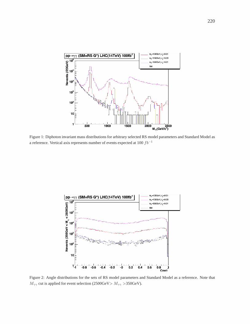
220

Figure 1: Diphoton invariant mass distributions for arbitrary selected RS model parameters and Standard Model as

a reference. Vertical axis represents number of events expected at 100fb−1

Figure 2: Angle distributions for the sets of RS model parameters and Standard Model as a reference. Note that

Mγγ cut is applied for event selection (2500GeV>Mγγ >350GeV).

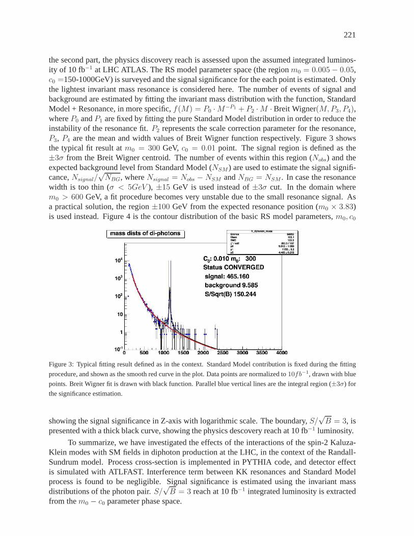
221

the second part, the physics discovery reach is assessed upon the assumed integrated luminos-ity of 10 fb−1 at LHC ATLAS. The RS model parameter space (the regionm0 = 0.005 − 0.05,c0 =150-1000GeV) is surveyed and the signal significance for theeach point is estimated. Onlythe lightest invariant mass resonance is considered here. The number of events of signal andbackground are estimated by fitting the invariant mass distribution with the function, StandardModel + Resonance, in more specific,f(M) = P0 ·M−P1 + P2 ·M ·Breit Wigner(M,P3, P4),whereP0 andP1 are fixed by fitting the pure Standard Model distribution in order to reduce theinstability of the resonance fit.P2 represents the scale correction parameter for the resonance,P3, P4 are the mean and width values of Breit Wigner function respectively. Figure 3 showsthe typical fit result atm0 = 300 GeV, c0 = 0.01 point. The signal region is defined as the±3σ from the Breit Wigner centroid. The number of events within this region (Nobs) and theexpected background level from Standard Model (NSM ) are used to estimate the signal signifi-cance,Nsignal/

√NBG, whereNsignal = Nobs − NSM andNBG = NSM . In case the resonance

width is too thin (σ < 5GeV ), ±15 GeV is used instead of±3σ cut. In the domain wherem0 > 600 GeV, a fit procedure becomes very unstable due to the small resonance signal. Asa practical solution, the region±100 GeV from the expected resonance position (m0 × 3.83)is used instead. Figure 4 is the contour distribution of the basic RS model parameters,m0, c0

Figure 3: Typical fitting result defined as in the context. Standard Model contribution is fixed during the fitting

procedure, and shown as the smooth red curve in the plot. Datapoints are normalized to10fb−1, drawn with blue

points. Breit Wigner fit is drawn with black function. Parallel blue vertical lines are the integral region (±3σ) for

the significance estimation.

showing the signal significance in Z-axis with logarithmic scale. The boundary,S/√B = 3, is

presented with a thick black curve, showing the physics descovery reach at 10 fb−1 luminosity.

To summarize, we have investigated the effects of the interactions of the spin-2 Kaluza-Klein modes with SM fields in diphoton production at the LHC, in the context of the Randall-Sundrum model. Process cross-section is implemented in PYTHIA code, and detector effectis simulated with ATLFAST. Interference term between KK resonances and Standard Modelprocess is found to be negligible. Signal significance is estimated using the invariant massdistributions of the photon pair.S/

√B = 3 reach at 10 fb−1 integrated luminosity is extracted

from them0 − c0 parameter phase space.

222

Figure 4: Signal significance distribution inm0 − c0 parameter phase space. The black curve shows the expected

discovery sensitivity boundary (S/√B = 3).

223

Part 32

Higgsless models of electroweak symmetrybreakingG. Cacciapaglia

AbstractHiggsless models are the most radical alternative to the SM,for theelectroweak symmetry is broken without any elementary scalar in thetheory. The scattering amplitude of longitudinal polarized gauge bosonsis unitarized by a tower of massive vector boson that replaces the SMHiggs boson. It is possible to write down a realistic theory in a warpedextra dimension, that satisfies the electroweak precision bounds. Themain challenge is to introduce the third generation of quarks, the topand bottom: there is indeed a tension between obtaining a heavy enoughtop and small deviations in the couplings of the bottom with theZ bo-son. This idea also offers a rich model independent phenomenology thatshould be accessible at LHC.

1. INTRODUCTION

The main theoretical prejudice against field theories with fundamental scalars, like the Higgsboson in the Standard Model, is the instability of their mass. If there is not any symmetryprotecting it, the radiative corrections to the mass parameter will be proportional to the cutoff,or to the scale where new physics has to be added to the theory.Thus, unless a large fine tuningis invoked, the SM description of EWSB is not satisfactory. The most radical approach to thisproblem is to built a theory where there is not any light scalar in the low energy spectrum, orHiggsless models.

If we remove the Higgs from the SM, the first problem we run intois the scattering of thelongitudinally polarizedW bosons: the tree level amplitude grows like the energy square andat some energy scale (around1.8 TeV in the SM) we lose control of the perturbation expansion.The role of the Higgs is to cancel such divergent term. Historically, the first approach was toassume that strong coupling indeed occurs around1 TeV, and that it is the strong dynamicsitself to induce the gauge symmetry breaking: this is the idea of technicolour. However, thesemodels have serious problems in accommodating the electroweak precision tests performed atLEP in the last decade: generically they predict large deviations, and the lack of calculabilitydoes not allow to decide if this scenario is definitely ruled out. Is it possible to build a Higgslessmodel where the loss of perturbative control occurs at energies larger that a TeV? The easiestpossibility is to add a massive vector particle, with mass inthe TeV range, that cancels thequadratically growing term in the scattering amplitude. However, the scattering amplitude ofthe new heavy boson will grow quadratically in the energy again, thus incurring in a strongcoupling regime at a higher energy than before. If we want to keep playing this game, we canadd another massive vector boson, and so on. The cancellation of the growing terms in theamplitude will impose sum rules on the couplings and masses of the new heavy states. For

224

instance, from theWLWL scattering:

gWWWW = e2 + g2WWZ +

∑

k

g2WWk ; (1)

gWWWW =3

4

(

g2WWZ

M2Z

M2W

+∑

k

g2WWk

M2k

M2W

)

. (2)

The first sum rule ensures the cancellation of a term growing with the fourth power of theenergy, whose cancellation in the SM is ensured by gauge invariance that relates the couplings.In Refs. [609–616], it has been shown that these sum rules areautomatically satisfied in Yang-Mills theories in extra dimensional spaces, where the gaugesymmetries are broken by suitableboundary conditions. Namely, one can impose that the gauge fields associated with the brokengenerators vanish on the boundaries of the extra dimension,so that all the modes associatedwith such fields are massive. It is also possible to write 4 dimensional theories with the sameproperty: these are the so called moose models, or deconstructed extra dimensions [488]. Theidea is to latticize the extra dimension, and replace it witha finite number of replicas of thegauge group. Scalar links will provide the breaking of theN gauge groups. Higgsless modelshave been proposed both in the 5 dimensional case in Refs. [550,617,618], and further studiedin Refs. [556, 619–625], and in 4 dimensions in Refs. [626–628] (see also Refs. [629–642]).In the rest of this review, we will focus on the extra dimensional attempts, however, the sameconclusions apply to the 4 dimensional models. The only difference is that the deconstructedmodels are less constrained, as they explicitly violate 5D Lorentz invariance.

1.1 A ONE PAGE MINICOURSE IN EXTRA DIMENSIONS

If we were to consider the existence of an extra spatial dimension, in order to hide it at lowenergies we need to compactify it, so that it will be negligible at energies below its typicallength. The simplest way to imagine it, is to think in terms ofan interval. Any fieldΦ will alsodepend on the extra coordinatez: we can reduce the theory to a 4 dimensional one if we Fourierexpand the fields in the extra component, namely

Φ(xµ, z) =∑

k

fk(z)φk(xµ) ; (3)

where a 4D fieldφk is associated to each frequency of the interval. The massmk of these infinitefields will be determined by the boundary conditions at the interval endpoints, and are like theenergy required to excite that particular frequency.

In order to make this statement more clear, we will focus on a simple gauge theory in a flatextra dimension. In this case, the 5D vector has an extra component along the extra direction

A = (Aµ, A5) . (4)

However, not all the modes in the 4D scalarA5 are physical: indeed they can be gauged away,and they will play the role of the longitudinal modes of the massive vectors resulting from the4D reduction described above. The simplest boundary condition that can be imposed on thissystem are Neumann, namely the vanishing of the derivative along the extra component onthe interval endpoints∂5Aµ = 0. These BCs allows for a constant solutionf0 = const, that

225

corresponds to a massless vector26. From the 4D point of view, the bulk gauge symmetry isunbroken. The massive states will have masses given byn/L, L being the length of the intervalandn an integer.

Another possibility is to impose Dirichlet BCs for the vector components: in this case theflat solution is not allowed and all the vector states are massive. This signals that the gaugesymmetry is also broken in 4D. However, the choice of BCs is not completely arbitrary, as notall the possibilities will lead to a unitary theory: the sum rules advocated above will be satisfiedonly for a healthy choice. It turns out that healthy BCs come from a spontaneous breaking ofthe symmetry on the boundaries. In order to see it, we can add to the theory a scalar degreeof freedom localized on one of the two endpoints, and assume that it will develop a vacuumexpectation value as for the SM Higgs. The Neumann BC will be modified to:

∂5Aµ ± g2v2

4Aµ = 0 , (5)

wherev is the VEV and the sign corresponds to the choice of endpoint.For small VEV, themass of the gauge boson is proportional togv. However, in the limit of largev, the mass of thefirst massive state is given by1/(2L): this corresponds to switching the BC to Dirichlet BCs. Ifwe play this trick on both the endpoints, the first state will have mass1/L, however in this casethe BCs forA5 will allow for a scalar massless state that cannot be gauged away. Indeed, weare breaking the symmetry twice, with two separate Higgs sectors: thus only one combinationof the two resulting goldstone bosons is eaten by the massivevectors, the other one is a physicalmassless scalar.

2. THE MODEL

We will consider the model proposed in Refs. [550, 623]: a SU(2)L×SU(2)R×U(1)B−L gaugetheory on a AdS5 background, i.e. one extra dimension with a warped metric [470]. Theconformally flat metric on AdS can be parametrized as:

ds2 =

(R

z

)2(ηµνdx

µdxν − dz2), (6)

where the extra coordinatez is on the interval[R,R′]. The curvatureR is usually assumed to beof order1/MP l, but in this case it will be a free adjustable parameter. The physical interpretationof this metric is that the unit length, or equivalently the energy scale, depends on the positionin the extra dimension. On thez = R endpoint, the Planck brane, it is of order1/R, while onthez = R′ endpoint, the TeV brane, it is warped down to the smaller scale 1/R′, that we willassume to be of order the weak scale. The bulk gauge symmetry is broken on the boundariesof the extra dimension: on the Planck brane we will preserve the SM gauge group, so thatthe breaking pattern is SU(2)R×U(1)B−L → U(1)Y . On the TeV brane, on the other hand,we will break the two SU(2)’s to the diagonal one SU(2)L×SU(2)R →SU(2)D 27. As alreadymentioned, the breaking is realized imposing Dirichlet BC’s for the broken generators28. If we

26Note that the BCs forA5 are forced to be Dirichlet, i.e. vanishing of the field, thus there is not any masslessscalar mode. All the modes inA5 are then gauged away.

27Note that in the SM this same symmetry breaking is induced by the Higgs, where SU(2)R is a global symmetryin the gauge sector.

28With this choice, there is not any symmetry broken on both branes, thus all the scalar modes are eaten.

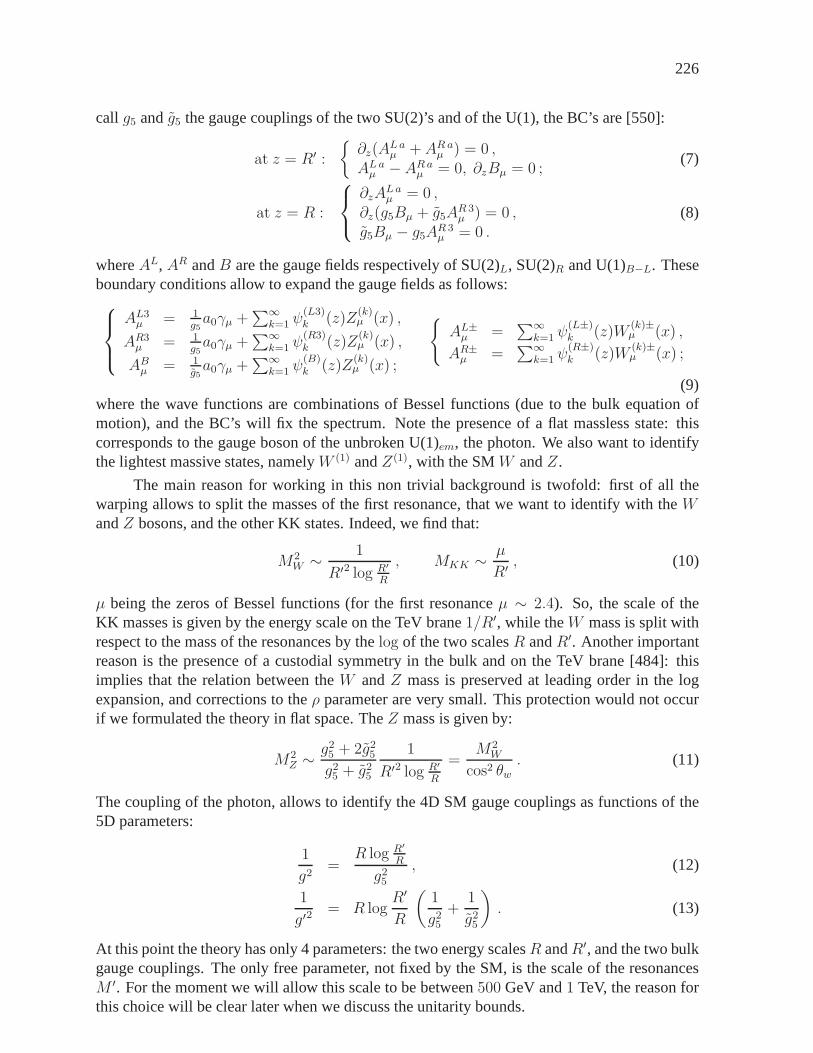
226

call g5 andg5 the gauge couplings of the two SU(2)’s and of the U(1), the BC’s are [550]:

at z = R′ :

∂z(A

Laµ + ARaµ ) = 0 ,

ALaµ − ARaµ = 0, ∂zBµ = 0 ;(7)

at z = R :

∂zALaµ = 0 ,

∂z(g5Bµ + g5AR 3µ ) = 0 ,

g5Bµ − g5AR 3µ = 0 .

(8)

whereAL, AR andB are the gauge fields respectively of SU(2)L, SU(2)R and U(1)B−L. Theseboundary conditions allow to expand the gauge fields as follows:

AL3µ = 1

g5a0γµ +

∑∞k=1 ψ

(L3)k (z)Z

(k)µ (x) ,

AR3µ = 1

g5a0γµ +

∑∞k=1 ψ

(R3)k (z)Z

(k)µ (x) ,

ABµ = 1g5a0γµ +

∑∞k=1 ψ

(B)k (z)Z

(k)µ (x) ;

AL±µ =∑∞

k=1 ψ(L±)k (z)W

(k)±µ (x) ,

AR±µ =∑∞

k=1 ψ(R±)k (z)W

(k)±µ (x) ;

(9)where the wave functions are combinations of Bessel functions (due to the bulk equation ofmotion), and the BC’s will fix the spectrum. Note the presenceof a flat massless state: thiscorresponds to the gauge boson of the unbroken U(1)em, the photon. We also want to identifythe lightest massive states, namelyW (1) andZ(1), with the SMW andZ.

The main reason for working in this non trivial background istwofold: first of all thewarping allows to split the masses of the first resonance, that we want to identify with theWandZ bosons, and the other KK states. Indeed, we find that:

M2W ∼ 1

R′2 log R′

R

, MKK ∼ µ

R′ , (10)

µ being the zeros of Bessel functions (for the first resonanceµ ∼ 2.4). So, the scale of theKK masses is given by the energy scale on the TeV brane1/R′, while theW mass is split withrespect to the mass of the resonances by thelog of the two scalesR andR′. Another importantreason is the presence of a custodial symmetry in the bulk andon the TeV brane [484]: thisimplies that the relation between theW andZ mass is preserved at leading order in the logexpansion, and corrections to theρ parameter are very small. This protection would not occurif we formulated the theory in flat space. TheZ mass is given by:

M2Z ∼ g2

5 + 2g25

g25 + g2

5

1

R′2 log R′

R

=M2

W

cos2 θw. (11)

The coupling of the photon, allows to identify the 4D SM gaugecouplings as functions of the5D parameters:

1

g2=

R log R′

R

g25

, (12)

1

g′2= R log

R′

R

(1

g25

+1

g25

)

. (13)

At this point the theory has only 4 parameters: the two energyscalesR andR′, and the two bulkgauge couplings. The only free parameter, not fixed by the SM,is the scale of the resonancesM ′. For the moment we will allow this scale to be between500 GeV and1 TeV, the reason forthis choice will be clear later when we discuss the unitaritybounds.

227

The major stumbling block for any theory beyond the SM is the level of correctionsto Electroweak Precision measurements, mainly performed by LEP1 at the Z pole, and byLEP2 [450, 643]. In the following we will focus on the old parametrization by Peskin andTakeuchi [644]: in universal theories the corrections to Z pole observables can be described byonly 3 parameters, calledS, T andU . Another kind of corrections are given by 4-fermi oper-ators induced at tree level by the exchange of the massive gauge bosons, and we will commenton them separately29. The parameterU is generically small, corresponding to a higher orderoperator in the effective lagrangean, so we will neglect it.The parameterT can be directlyrelated to the corrections to the relation between theW andZ mass: as already mentioned, thecustodial symmetry built in this model will protect this parameter from large corrections. Thus,the parameterS is the worrisome one. In order to compute it, we must specify the fermion con-tent of the theory, as it also depends on the couplings between gauge bosons and light fermions.The simplest choice is to localize the light fermions on the Planck brane [618, 621]: the reasonis that the SM gauge group is unbroken there, so we will not introduce non-standard couplings,and eventual flavour changing neutral currents will be suppressed by a large scale1/R. In thislimit, the leading contribution toS is given by:

S ∼ 6π

g2 log R′

R

=6π

g2

(

2.4MW

M ′

)2

∼ 1.9

(1 TeVM ′

)2

. (14)

This value is large and positive, similar to the one found in traditional technicolour theories,and it is too big compared with the experimental limit|S| ≤ 0.3. A more complete analysis ofthis model, including the effect of localized terms, shows that precision data highly disfavourthe model with localized fermions [232].

The solution to this problem is to relax the assumptions of localized fermions, as proposedin Refs. [623,628] and further studied in Refs. [625,636–638]: this will also have another crucialbeneficial effect regarding the direct bounds on light gaugebosons. It has been known for a longtime in Randall-Sundrum (RS) models with a Higgs that the effectiveS parameter is large andnegative [645] if the fermions are localized on the TeV braneas originally proposed [470].When the fermions are localized on the Planck brane the contribution toS is positive, and sofor some intermediate localization theS parameter vanishes, as first pointed out for RS modelsby Agashe et al. [484]. The reason for this is fairly simple. Since theW andZ wave functionsare approximately flat, and the gauge KK mode wave functions are orthogonal to them, whenthe fermion wave functions are also approximately flat the overlap of a gauge KK mode withtwo fermions will approximately vanish. Since it is the coupling of the gauge KK modes to thefermions that induces a shift in theS parameter, for approximately flat fermion wave functionstheS parameter must be small. Note that not only does reducing thecoupling to gauge KKmodes reduce theS parameter, it also weakens the experimental constraints onthe existence oflight KK modes. This case of delocalized bulk fermions is notcovered by the no–go theoremof [232], since there it was assumed that the fermions are localized on the Planck brane.

In order to quantify these statements, it is sufficient to consider a toy model where all thethree families of fermions are massless and have a universaldelocalized profile in the bulk [623].We first briefly review the bulk equation of motion in AdS5. In 5D fermions are vector-like, so

29Recently Barbieriet al proposed a new generalized set of parameters [232], that takes into account the datafrom LEP2, namely the 4 fermi operators.

228

that they contain both a left- and right-handed component:

Ψ =

(χψ

)

, (15)

where the boundary conditions can be chosen such that there is a zero mode either in the left–handed (lh) or in the right–handed (rh) component. The wave function of the zero mode will bedetermined by the bulk mass term, that we parametrize byc in units ofR. If the zero mode islh, the solution of the bulk equations of motion is:

χ0 = A0

( z

R

)2−c. (16)

Studying the above profile, it’s easy to show that lh (rh) fermions are localized on the Planckbrane ifc > 1/2 (c < −1/2), else on the TeV brane, while forc = 1/2 (c = −1/2) the profileis flat.

Now, the gauge couplings of the fermions will depend on the parameterc through the bulkintegral of the gauge boson wave functions. For a lh fermion,that transforms under the bulkgauge group as a2L × 1R × qB−L representation, it reads:

a0 Qγµ + g5 IL∓l (c)TL±W∓µ + g5 I(L3)

l (c)

(

TL3 +g5 I(B)

l (c)

g5 I(L3)l (c)

Y

2

)

Zµ , (17)

where we have used thatY/2 = QB−L (for SU(2)R singlets) and the electric charge is definedasQ = Y/2 + TL3, and:

IXl (c) = A20

∫ R′

R

dz

(R

z

)2 c

φX1 (z) . (18)

Only the electric charge does not depend on the fermion profile, as the massless photon is flatalong the extra dimension. However, the couplings to theW andZ are affected in a universalway: the corrections can be cast into the definition of the oblique parameters and yield aneffective shift ofS.

In order to do that, we have to impose the following matching condition between the 4Dcouplings and the 5D parameters of the theory30:

tan2 θW =g′2

g2= − g5 I(B)

l (cL)

g5 I(L3)l (cL)

, (19)

while the matching of the electric charge remains unaffected:

1

e2=

1

a20

=

(1

g25

+2

g25

)

R logR′

R. (20)

Now, we can recalculateS taking into account this shift: in the limit wherec ∼ 1/2, so that thefermion profile is almost flat, the leading contributions toS are:

30Note that this equation does not depend on the overall normalization of theZ wave function, but is completelydetermined by the boundary conditions in eqs. (7–8).

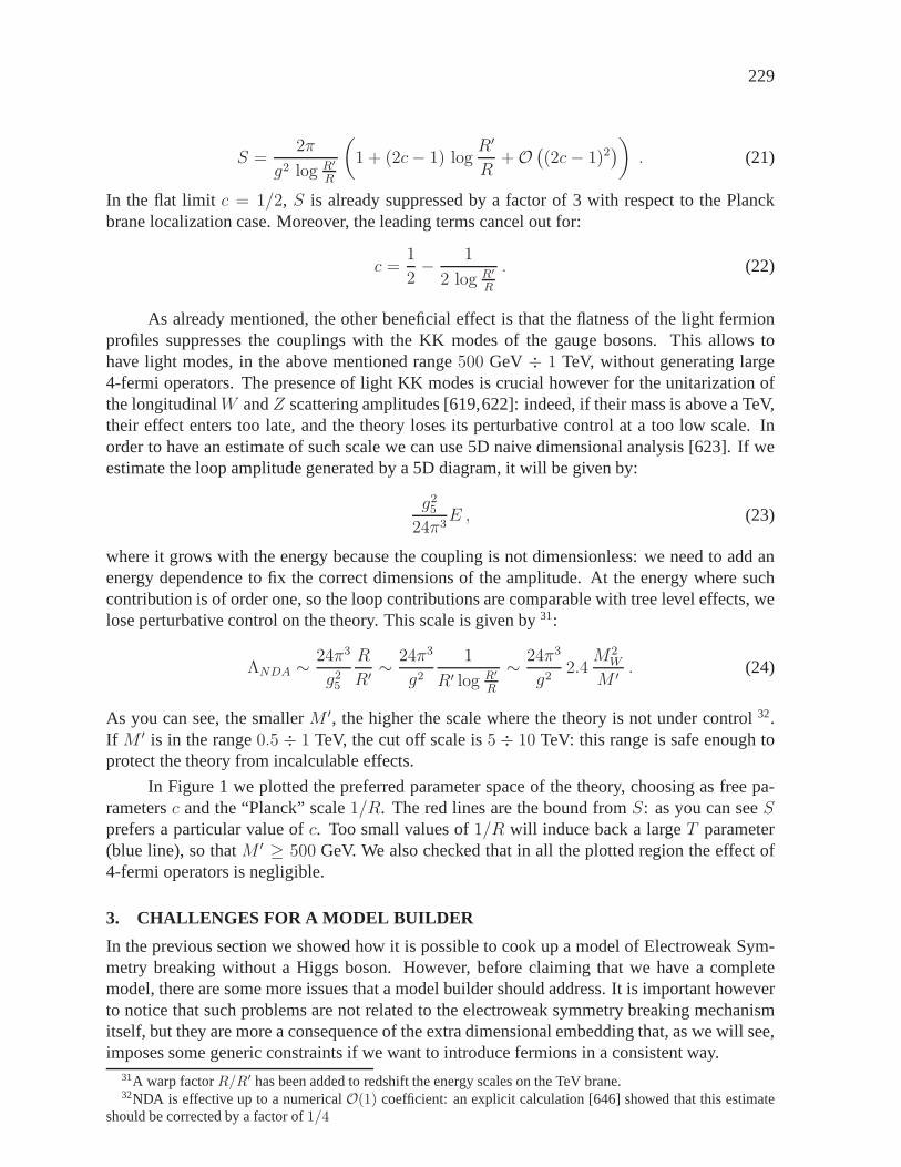
229

S =2π

g2 log R′

R

(

1 + (2c− 1) logR′

R+ O

((2c− 1)2

))

. (21)

In the flat limit c = 1/2, S is already suppressed by a factor of 3 with respect to the Planckbrane localization case. Moreover, the leading terms cancel out for:

c =1

2− 1

2 log R′

R

. (22)

As already mentioned, the other beneficial effect is that theflatness of the light fermionprofiles suppresses the couplings with the KK modes of the gauge bosons. This allows tohave light modes, in the above mentioned range500 GeV ÷ 1 TeV, without generating large4-fermi operators. The presence of light KK modes is crucialhowever for the unitarization ofthe longitudinalW andZ scattering amplitudes [619,622]: indeed, if their mass is above a TeV,their effect enters too late, and the theory loses its perturbative control at a too low scale. Inorder to have an estimate of such scale we can use 5D naive dimensional analysis [623]. If weestimate the loop amplitude generated by a 5D diagram, it will be given by:

g25

24π3E , (23)

where it grows with the energy because the coupling is not dimensionless: we need to add anenergy dependence to fix the correct dimensions of the amplitude. At the energy where suchcontribution is of order one, so the loop contributions are comparable with tree level effects, welose perturbative control on the theory. This scale is givenby 31:

ΛNDA ∼ 24π3

g25

R

R′ ∼24π3

g2

1

R′ log R′

R

∼ 24π3

g22.4

M2W

M ′ . (24)

As you can see, the smallerM ′, the higher the scale where the theory is not under control32.If M ′ is in the range0.5 ÷ 1 TeV, the cut off scale is5 ÷ 10 TeV: this range is safe enough toprotect the theory from incalculable effects.

In Figure 1 we plotted the preferred parameter space of the theory, choosing as free pa-rametersc and the “Planck” scale1/R. The red lines are the bound fromS: as you can seeSprefers a particular value ofc. Too small values of1/R will induce back a largeT parameter(blue line), so thatM ′ ≥ 500 GeV. We also checked that in all the plotted region the effectof4-fermi operators is negligible.

3. CHALLENGES FOR A MODEL BUILDER

In the previous section we showed how it is possible to cook upa model of Electroweak Sym-metry breaking without a Higgs boson. However, before claiming that we have a completemodel, there are some more issues that a model builder shouldaddress. It is important howeverto notice that such problems are not related to the electroweak symmetry breaking mechanismitself, but they are more a consequence of the extra dimensional embedding that, as we will see,imposes some generic constraints if we want to introduce fermions in a consistent way.

31A warp factorR/R′ has been added to redshift the energy scales on the TeV brane.32NDA is effective up to a numericalO(1) coefficient: an explicit calculation [646] showed that thisestimate

should be corrected by a factor of1/4

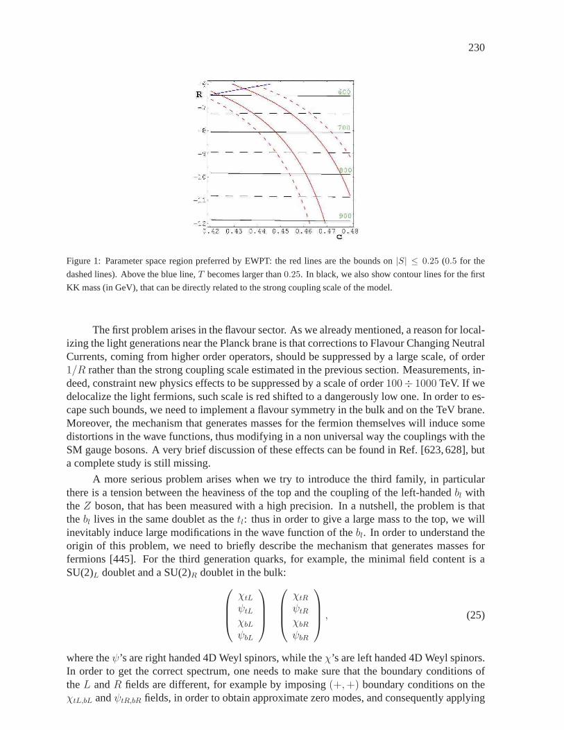
230

Figure 1: Parameter space region preferred by EWPT: the red lines are the bounds on|S| ≤ 0.25 (0.5 for the

dashed lines). Above the blue line,T becomes larger than0.25. In black, we also show contour lines for the first

KK mass (in GeV), that can be directly related to the strong coupling scale of the model.

The first problem arises in the flavour sector. As we already mentioned, a reason for local-izing the light generations near the Planck brane is that corrections to Flavour Changing NeutralCurrents, coming from higher order operators, should be suppressed by a large scale, of order1/R rather than the strong coupling scale estimated in the previous section. Measurements, in-deed, constraint new physics effects to be suppressed by a scale of order100÷ 1000 TeV. If wedelocalize the light fermions, such scale is red shifted to adangerously low one. In order to es-cape such bounds, we need to implement a flavour symmetry in the bulk and on the TeV brane.Moreover, the mechanism that generates masses for the fermion themselves will induce somedistortions in the wave functions, thus modifying in a non universal way the couplings with theSM gauge bosons. A very brief discussion of these effects canbe found in Ref. [623, 628], buta complete study is still missing.

A more serious problem arises when we try to introduce the third family, in particularthere is a tension between the heaviness of the top and the coupling of the left-handedbl withtheZ boson, that has been measured with a high precision. In a nutshell, the problem is thatthebl lives in the same doublet as thetl: thus in order to give a large mass to the top, we willinevitably induce large modifications in the wave function of the bl. In order to understand theorigin of this problem, we need to briefly describe the mechanism that generates masses forfermions [445]. For the third generation quarks, for example, the minimal field content is aSU(2)L doublet and a SU(2)R doublet in the bulk:

χtLψtLχbLψbL

χtRψtRχbRψbR

, (25)

where theψ’s are right handed 4D Weyl spinors, while theχ’s are left handed 4D Weyl spinors.In order to get the correct spectrum, one needs to make sure that the boundary conditions oftheL andR fields are different, for example by imposing(+,+) boundary conditions on theχtL,bL andψtR,bR fields, in order to obtain approximate zero modes, and consequently applying

231

the opposite(−,−) boundary conditions to the remaining fields. A Dirac mass

MDR′(χtLψtR + χbLψbR) (26)

can be added on the TeV brane. Due to the remainingSU(2)D gauge symmetry the same termhas to be added for top and bottom quarks. The necessary splitting between top and bottom canthen be achieved by modifying the BC’s on the Planck brane, where the SU(2)R is broken: forinstance we can add a large brane induced kinetic term forψbR [618].

For cL ∼ 0.5 (or larger) it is impossible to obtain a heavy enough top quark mass. Thereason is that forMDR

′ ≫ 1 the light mode mass saturates at

m2top ∼

2

R′2 log R′

R

, (27)

which gives for this casemtop ≤√

2MW . Thus one needs to localize the top and the bottomquarks closer to the TeV brane. However, even in this case a sizable Dirac mass term on theTeV brane is needed to obtain a heavy enough top quark. The consequence of this mass term isthe boundary condition for the bottom quarks

χbR = MDR′ χbL. (28)

This implies that ifMDR′ ∼ 1 then the left handed bottom quark has a sizable component also

living in anSU(2)R multiplet, which however has a coupling to theZ that is different from theSM value. Thus there will be a large deviation in theZblbl.

A possible way out would be to increase the scale1/R′: in this way a smallMDR′ should

be enough to reproduce the top mass without also inducing large mixings in the b sector [623,628]. However, in the simple realization the scale of1/R′ is related to theW mass. A possibilitystudied in Ref. [624] is to introduce twoR′ scales, one related to theW mass and one to thetop mass: this is possible introducing two AdS spaces and matching them on the Planck brane.However, in this scenario a strong coupling will necessarily arise in the top sector, thus affectingthe predictive power of the model in the top sector.

Another interesting possibility would be to realize the custodial symmetry in a differentway. So far, we assumed that the right-handed components of the top and bottom form a doubletof SU(2)R. An alternative would be to assume that thetr is a singlet, and the left-handed doubletis part of a bidoublet of SU(2)L×SU(2)R. In this way it is possible to write different SU(2)D

invariant masses for the top and bottom on the TeV brane. However, the new BC’s will also giverise to a lighter top, so that it is necessary to localize the fields more closely to the TeV brane.

Another generic problem arising from the large value of the top-quark mass in modelswith warped extra dimensions comes from the isospin violations in the KK sector of the top andthe bottom quarks [472]. If the spectrum of the top and bottomKK modes is not sufficientlydegenerate, the loop corrections involving these KK modes to theT -parameter could be large.However, the precise value of these corrections crucially depends on how the third generationis realized.

Finally, we should note that this tension in the top sector isreally a consequence of theextra dimensional setup. In the deconstructed model of Refs. [642] this problem can be eas-ily solved modifying the couplings of fermions in differentpoints of the lattice points. Fromthe extra dimensional point of view, this would correspond to terms that are not 5D Lorentzinvariant.

232

4. PHENOMENOLOGY AND COLLIDER SIGNATURE

Many different realizations of Higgsless models have been proposed in the literature, differingin the way fermions are introduced and if formulated in an extra dimensional framework or indeconstruction or moose theories. Such models would lead todifferent experimental signatures.However, the fundamental mechanism that leads to a delay in the scale where the strong cou-pling breaks the electroweak symmetry is common to all of these models. A model independentprediction is the presence of massive vector bosons that will couple with theW andZ andcontribute to the unitarization of the longitudinal mode scattering via sum rules like the ones inEqs. (1) and (2). Thus, it is possible to identify some signatures at colliders that are typical ofHiggsless models, and can be used to probe and discriminate this proposal with respect to othermodels.

We will again concentrate on the extra dimensional realization of the Higgsless mech-anism described above, but the featured pointed here can be easily extended to all the otherproposals. In order to have an efficient unitarization, namely a large enough scale of strongcoupling, we need the first resonances to be below1 TeV. Moreover, their couplings with theSM W andZ have to obey the sum rules: generically the sum rules are satisfied with a highprecision by the inclusion of only the first (few) resonances. Another common feature, requiredby the smallness of oblique corrections, theS parameter, is the smallness of the couplings withthe light SM fermions. This observation allows to simplify the phenomenology of the model:indeed we can neglect the couplings with the light fermions,that are model dependent, and onlyconsider the couplings with the gauge bosons. A crucial prediction is again the sum rules: itwould be important to measure precisely enough the masses and couplings and check the sumrules. A preliminary study in this direction has been performed in Ref. [647]. The authors focuson theW − Z scattering, because it is easier to measure at hadron colliders. In this channelsimilar sum rules apply:

gWWZZ = g2WWZ +

∑

k

g2WZk, (29)

(gWWZZ − g2WWZ)(M2

W +M2Z) + g2

WWZ

M4Z

M2W

=∑

k

g2WZk

[

3(M±k )2 − (M2

Z −M2W )2

(M±k )2

]

.(30)

This channel is more appealing because it predicts the presence of charged resonances, and thefinal state is more easily disentangled from the background.

In Figure 2 we show the number of events expected in a 300 fb−1 LHC data sample,as a function of theWZ invariant massmWZ . The Higgsless model should be easily seenvia a narrow resonance. For comparison, they also studied two unitarization models, relyingon strong coupling at a TeV scale. The analysis in the paper shows that, assuming that theproduction channel is only via gauge boson fusion, LHC at full luminosity should be able toprobe all the interesting mass scales for the resonances.

However, at LHC it will not be possible to measure the couplings in order to check thesum rules. A more sophisticated analysis should also include the couplings to the fermions:indeed the Drell-Yan production mechanism should be much more effective. Moreover, thedecay channel of theZ ′ in dileptons should make very easy to discover such resonances. Asalready stresses, such statements depend on the fermion content: as you can see from Figure 1,the smallness of theS parameters highly constraints the parameter space. Thus, if we stickwith this minimal model, it should be possible to predict thecouplings with fermions, and thus

233

Figure 2: The number of events per 100 GeV bin in the2j+3l+ν channel at the LHC with an integrated luminosity

of 300 fb−1 and cuts as indicated in the figure. The different histogramscorrespond to the Higgsless model (blue)

with a resonance at700 GeV, and two ”unitarization” models: Pade (red) and K-matrix (green). (From Ref. [647])

include this effect into the analysis. A combination in the measurements of the decay channelsinto dileptons and gauge bosons may allow to measure the couplings even at LHC.

Figure 3: Deviations in theWWZ (left) andWWWW (right) gauge couplings in the Higgsless model as a

function ofc andR. The red and blue lines are the regions preferred byS andT , as in Figure 1. The percentage

deviation (w.r.t. the SM values) are negative.

Another interesting prediction of Higgsless models is the presence of anomalous 4- and 3-boson couplings. Indeed, in the SM the sum rules canceling the terms growing with the fourthpower of the energy are already satisfied by gauge invariance. In order to accommodate thecontribution of the new states, the couplings between SM gauge bosons have to be corrected.Assuming that the sum rules are satisfied by the first level it is easy to evaluate such deviations:

δgWWZ

gWWZ∼ −1

2

M2W

M ′Z

2 − 2∆ ,δgWWWW

gWWWW∼ −3

4

M2W

M ′Z

2 − 2∆ ; (31)

234

whereg2WW1/gWWWW ∼ 1/4M2

W/M2Z′ + ∆ in order to satisfy the second sum rule in Eq. 2.

In Figure 3 we plotted the deviations in theWWWW andWWZ gauge couplings inthe Higgsless model described in these proceedings: the redlines encircle the preferred regionby EWPTs (as in Figure 1). As you can see, a deviation of order−1 ÷ 3 % is expected in thetrilinear gauge couplings. This deviation is close to the present experimental bound, coming bymeasurements at LEP, and might be probed by LHC. A linear collider (ILC) will surely be ableto measure such deviations: here we stress again that such deviations are a solid predictions ofthe Higgsless mechanism and are independent on the details of the specific Higgsless model weare interested in.

5. CONCLUSIONS

The most radical alternative to the SM Higgs mechanism is a theory where gauge symmetrybreaking takes place without a scalar particle. In this case, the scattering amplitude of longitu-dinal modes is unitarized by the presence of a tower of massive vector bosons. Such mechanismnaturally arises in extra dimensional theories, where the gauge symmetry breaking is inducedby the boundary conditions of gauge fields. The most realistic of such models is embedded in awarped background, thus ensuring a splitting between theW andZ masses and the masses ofthe resonances. A custodial symmetry is necessary in the bulk in order to protect theρ param-eter from large tree level corrections. Flat zero mode fermions also ensure the smallness of theother oblique correction, and a quasi-decoupling with the resonances. The latter property allowsfor light resonances, light enough to unitarize the theory up to5 ÷ 10 TeV and still allowed bydirect and indirect searches. The main challenge for model builders is to consistently includethe third generation. The problem is a tension between a large top quark and small correctionsto the coupling of the left-handed bottom with theZ boson. Moreover, the weak isospin vio-lation in this sector might induce unacceptably large one loop contributions to theρ parameter.We also mentioned some possibilities to overcome these problems.

It is also possible to write a deconstructed version of Higgsless theories: the main featuresare the same as in the extra dimensional realization. The main difference being that the absenceof 5D Lorentz invariance allows to have a heavy enough top.

Notwithstanding some theoretical problems of these models, the Higgsless mechanismleads to precise and model independent signatures. In particular, the gauge boson resonancesthat enter the unitarization ofW andZ scattering would be detected at LHC. Moreover, devi-ations in the tri-boson couplings are also required by the sum rules at a level near the presentbounds.

Acknowledgements

This research is supported by the NSF grant PHY-0355005.

235

Part 33

Resonant vector boson scattering at highmass at the LHCG. Azuelos, P-A. Delsart and J. Idarraga

AbstractWe examine, with full detector simuation, the reconstruction of WZresonances in the Chiral Lagrangian Model and the Higgslessmodel.

1. INTRODUCTION

In the absence of a light Higgs boson, either from the Standard Model (SM), from supersym-metry (MSSM), or from a Little Higgs model, electroweak symmetry breaking (EWSB) mustfind its origin in some strongly interacting sector. Since the Goldstone bosons (GB) breakingthe symmetry become the longitudinal components of the gauge bosons, the study of longitudi-nal vector boson (VL) scattering in the TeV region could reveal valuable information, hopefullyin the form of new resonances which should then be discoveredat the LHC. Previous ATLASstudies with full simulation can be found in [648,649]. Thisnote summarizes the main conclu-sions from an analysis of WZ resonances with a more realistic, full detector simulation [650],performed in the framework of the so-calledData-Challenge 2exercise of the ATLAS collabo-ration.

Dynamical EWSB is realized in many models, among which (i) models of technicolor,where a new QCD-like gauge interaction is introduced, alongwith chiral symmetry breakingproducing the required GB’s; extended, multiscale, top-color assisted models of technicolor arerequired to give mass to the fermions, including the top quark, while avoiding FCNC effects(for a review, see [533,651]); (ii) Little Higgs models [458,534], where a light Higgs is presentas a pseudo-GB resulting from the breaking of some specific higher symmetries, (iii) higgslessmodels [550], where EWSB results from boundary conditions at branes located in a warpedfifth space dimension, and (iv) string interactions. More generically, a Chiral Lagrangian (ChL)model [652–654] of EWSB provides a low energy effective description of electroweak interac-tions. It is built as a covariant momentum (derivative) expansion of GB fields, respecting thechiral symmetrySU(2)L × SU(2)R.

Here, we consider a 1.15 TeV resonance resulting from a chosen set of ChL parametersand a 700 GeV resonance from the Higgsless model.

2. Signals and backgrounds

The chiral Lagrangian, in its expansion to fourth order, consists of one term of dimension 2completely determined by the symmetry requirement and other interaction terms, of dimensionfour, with arbitrary coefficients, serving as parameters ofthe model (see the explicit form ofthe Lagrangian, for example, in [654,655]). Among the dimension-four terms, five of them de-scribe vector boson scattering, but only two of them, with coefficientsa4 anda5, are important ifone assumes that custodial symmetry is conserved. The parametersa4 anda5, together with theunitarization assumption, determine therefore the phenomenology of high energy longitudinal

236

vector boson scattering, and can lead to the presence or absence of resonances, as predicted byspecific models. The partial waves can be calculated and, since the effective Lagrangian is notrenormalizable, a unitarization procedure must be assumed. Here, we adopt the Inverse Ampli-tude Method (IAM), as described in [655]. It gives an excellent description of pion scatteringat low energies [656]. To generate Monte Carlo samples of this signal, we have modified pro-cess 73 of PYTHIA (WLZL scattering), replacing the partial waves by those for vector bosonscattering of the ChL model, as given in [260] and choosing the Pade unitarization, equivalentto the IAM. The parameters chosen werea4 = 0.00875 anda5 = −0.00125, corresponding topointP2 of ref [260], with a vector resonance of mass∼1150 GeV and widthΓ = 85 GeV.

The signal of the Higgsless model was generated with PYTHIA,using the QCD-likemodel of process 73, taking as reference a resonance mass of 700 GeV, as in [647, 657]. SMvector boson scattering background was added, choosingmh = 100 GeV in order to have anegligible contribution from diagrams with Higgs exchange. The normalization of the reso-nance was obtained by calculating the cross section in the resonance region in a model wheres-channel exchange of an additionalW1 Kaluza-Klein state of theW , of mass 700 GeV, wasintroduced and where the Higgs diagram was removed, as described in [647].

Three cases were studied: (i)qqWZ → qqjjℓℓ , (ii) qqWZ → qqℓνjj and (iii) qqWZ →qqℓνℓℓ. We discuss here only cases (1) and (3), as thett andW + j backgrounds are veryimportant in the second case. In the ChL and Higgsless models, for the cases studied, the crosssections forqqWZ production are respectively 91.2 fb and 180 fb.

The signals are characterized by the presence of theW andZ in the final state, but also oftwo high energy jets in the forward and backward directions originating from the primary quarksfrom which the gauge bosons have been radiated. The backgrounds, therefore, are processeswith vector bosons and at least two jets. We have considered the following because of their highcross-section.

• The main irreducible background is from SMqqWZ processes originating from gluon(QCD) orZ/γ (QED) exchange diagrams between quarks, with theW andZ radiatedfrom the quarks. The gauge bosons are mostly transverse (VT ), in this case, and emittedless centrally than in the case ofVLVL scattering. This background was generated withMADGraph [166] with some loose cuts: the two jets must havepT > 15 GeV, pseudo-rapidity |η| < 5, with separation|∆r(qq)| > 3, where∆r =

√

(∆φ)2 + (∆η), and theinvariant massmqq > 250 GeV. This leads to a cross section of 4.0 pb forqqW+Z and1.5 pb forqqW−Z.

• tt events withP topT > 500 GeV, generated with (MC@NLO). Although the transverse

momentum threshold is very high, the cross section is high (σ = 4.13 pb). The number ofevents used with full simulation, (18000), was therefore insufficient to assess with goodstatistical accuracy the importance of this background.

• W+4jets events. This background sample was produced with ALPGEN [176]. The cross-section isσ = 1200 pb and thus orders of magnitude above the signal.

All the events were fully simulated with Geant4 by the ATLAS collaboration, using AT-LAS Romeinitial detector layout (and using Athena version 9.0.4). They were digitized withelectronic noise but no-pileup. The events were reconstructed with the default settings (Athena10.0.4) but some extra jet collections were added (see following section).

237

3. ANALYSIS

Details of the analysis can be found in [650]. Here, we summarize the results, pointing out themain lessons from this full detector simulation study. The analysis was performed within theAthenaframework at the level of the Analysis Object Data (AOD). At this level, the potentialphysics objects (jets, muons, electrons,... ) are reconstructed and one can access their kinematicinformation as well as some identification or quality criteria.

We chose a set of cuts according to the signal caracteristicsdescribed in the introductionof the previous section :

1. identification and quality criteria . We impose an identification criterion (likelihood ora combinedIsEM variable) for the electrons. The leptons (e’s or µ’s) must have hightransverse momentum, 40 GeV and should be isolated, meaningthat there should be lessthan∼6 GeV of cumulated track energy in a 0.7 cone around their track. Once candidateelectrons or muons are chosen, jets, reconstructed by various algorithms, are accepted ifthey do not overlap with an electron and if they have a transverse momentumpT > 15GeV.

2. Forward jets. We require the presence of 2forward jetswith opposite directions. Weconsider a jet as a candidate forward jet if its transverse momentum is greater than 15GeV, energy greater than 200 GeV and if it satisfies one of the following conditions:

• It is the jetj1 with highest pseudorapidity (η), but is not also the jet with highestPT .• |ηj | > 2.5

• The difference|η| of this jet andj1 is: ∆ηjj1 > 4This complex selection was chosen in order to define central jets relative to forward jets(rather than with absoluteη cuts). Other algorithms for tagging the forward jets wereconsidered, but did not result in an overall improvement.

3. central jets Central jets expected from vector bosons are required to havepT > 40 GeV.They should lie, inη, between the two forward jets.

4. Vector boson mass. We impose that the mass of the reconstructed W and/or Z be in a±15 GeV window around the Standard Model value.

5. Central Jet Veto. We reject all events with any excess central jet (withpT > 40 GeV).6. ∆φ between vector bosonsDue to the high mass of the resonance, it is produced almost

at rest and the vector bosons are essentially back-to-back.We impose, therefore, that theybe well separated azimuthally:∆φWZ > 1.0.

7. Resonance mass. To evaluate the efficiencies of the selection criteria, we imposed awindow cut of±150 GeV (100 GeV for Higgsless case of a resonance at 700 GeV)around the reconstructed mass. The significance of the signal is then estimated from thenumber of signal (S) and background (B) events asS/

√B

One important characterisitic of the signal, for cases 1 and2, is that the two central jets fromthe energetic vector boson decays are highly boosted. They have a small opening angle andare often reconstructed as a single jet. To study this effectand account for it, we added tostandard reconstruction various sets of jets with different radius size. In general, if only one jetwas found, with mass close to the vector boson mass, we required that it be composed of twosubjets, when the cone radius was reduced to 0.2. Details canbe found in [650].

Preliminary results are shown in Fig 1 for the two signals considered. In both cases, astrong signal is seen, although the shape of the background must be well understood, especiallyfor the Higgsless resonance.

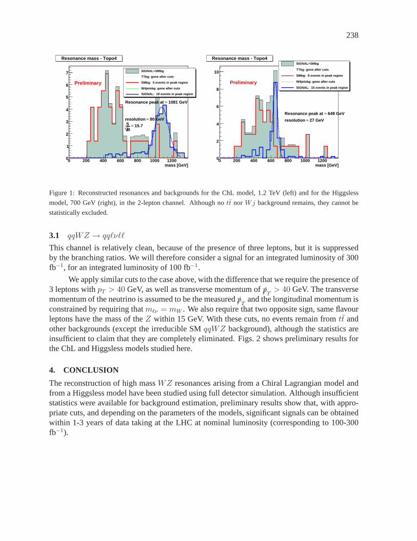
238

mass [GeV]0 200 400 600 800 1000 1200

310×0

1

2

3

4

5

6

7 SIGNAL+SMbg

TTbg: gone after cuts

SMbg: 5 events in peak region

W4jetsbg: gone after cuts

SIGNAL: 19 events in peak region

Resonance mass - Topo4

1081 GeV≈Resonance peak at

80 GeV≈resolution

15.7≈ BS

Preliminary

mass [GeV]0 200 400 600 800 1000 1200

310×0

2

4

6

8

10

SIGNAL+SMbg

TTbg: gone after cuts

SMbg: 8 events in peak region

W4jetsbg: gone after cuts

SIGNAL: 15 events in peak region

Resonance mass - Topo4

649 GeV≈Resonance peak at

27 GeV≈resolution

Preliminary

Figure 1: Reconstructed resonances and backgrounds for theChL model, 1.2 TeV (left) and for the Higgsless

model, 700 GeV (right), in the 2-lepton channel. Although nott norWj background remains, they cannot be

statistically excluded.

3.1 qqWZ → qqℓνℓℓ

This channel is relatively clean, because of the presence ofthree leptons, but it is suppressedby the branching ratios. We will therefore consider a signalfor an integrated luminosity of 300fb−1, for an integrated luminosity of 100 fb−1.

We apply similar cuts to the case above, with the difference that we require the presence of3 leptons withpT > 40 GeV, as well as transverse momentum of/pT > 40 GeV. The transversemomentum of the neutrino is assumed to be the measured/pT and the longitudinal momentum isconstrained by requiring thatmℓν = mW . We also require that two opposite sign, same flavourleptons have the mass of theZ within 15 GeV. With these cuts, no events remain fromtt andother backgrounds (except the irreducible SMqqWZ background), although the statistics areinsufficient to claim that they are completely eliminated. Figs. 2 shows preliminary results forthe ChL and Higgsless models studied here.

4. CONCLUSION

The reconstruction of high massWZ resonances arising from a Chiral Lagrangian model andfrom a Higgsless model have been studied using full detectorsimulation. Although insufficientstatistics were available for background estimation, preliminary results show that, with appro-priate cuts, and depending on the parameters of the models, significant signals can be obtainedwithin 1-3 years of data taking at the LHC at nominal luminosity (corresponding to 100-300fb−1).

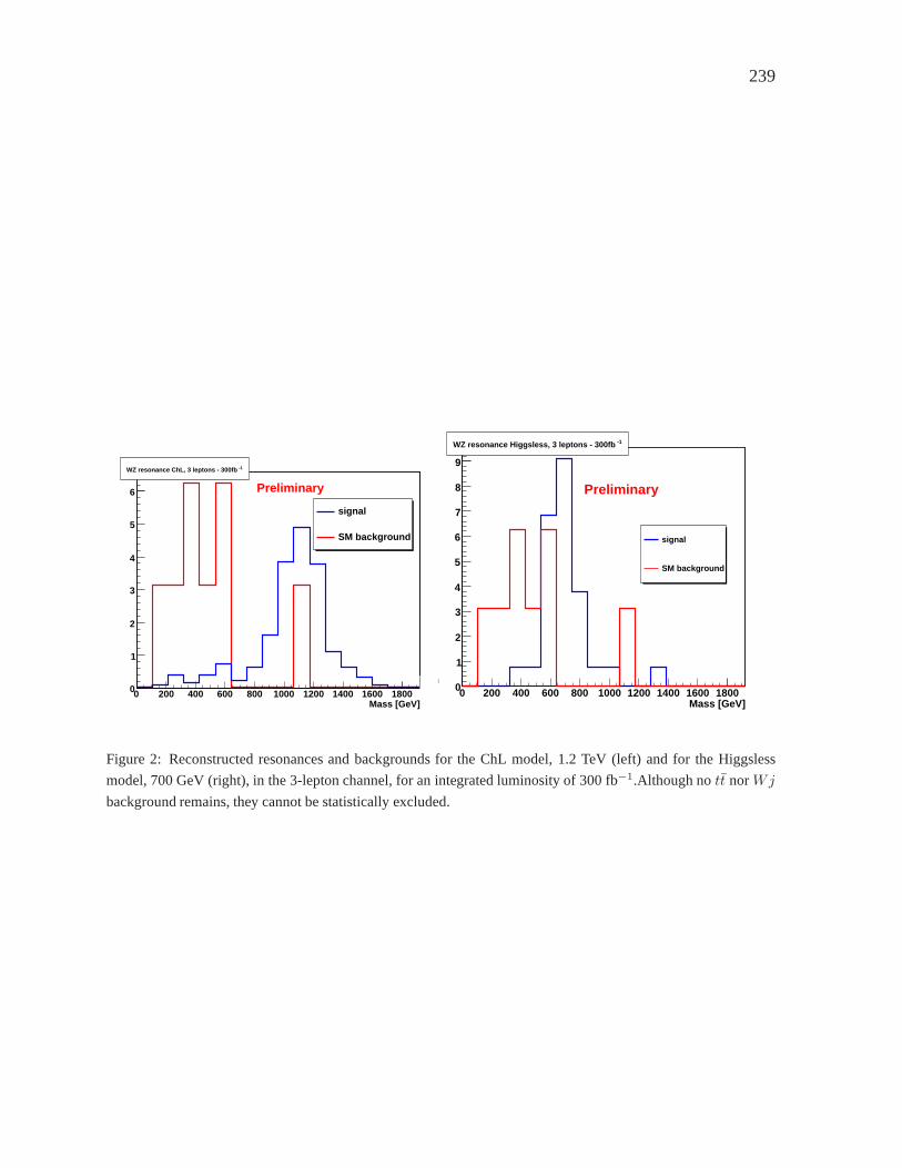
239

Mass [GeV]0 200 400 600 800 1000 1200 1400 1600 1800

310×0

1

2

3

4

5

6

-1WZ resonance ChL, 3 leptons - 300fb

signal

SM background

Preliminary

Mass [GeV]0 200 400 600 800 1000 1200 1400 1600 1800

310×0

1

2

3

4

5

6

7

8

9

-1WZ resonance Higgsless, 3 leptons - 300fb

signal

SM background

Preliminary

Figure 2: Reconstructed resonances and backgrounds for theChL model, 1.2 TeV (left) and for the Higgsless

model, 700 GeV (right), in the 3-lepton channel, for an integrated luminosity of 300 fb−1.Although nott norWj

background remains, they cannot be statistically excluded.

240

References

[1] H. Nilles, Phys. Rev.110(1984) 1.

[2] C. L. Bennettet. al., Astrophys. J. Suppl.148(2003) 1, [astro-ph/0302207 ].

[3] D. N. Spergelet. al.,, WMAP CollaborationAstrophys. J. Suppl.148(2003) 175,[astro-ph/0302209 ].

[4] J. R. Ellis, K. A. Olive, Y. Santoso, and V. C. Spanos,Phys. Lett.B565(2003) 176–182,[hep-ph/0303043 ].

[5] G. Belanger, F. Boudjema, A. Pukhov, and A. Semenov,Comput. Phys. Commun.149(2002) 103–120, [hep-ph/0112278 ].

[6] G. Belanger, F. Boudjema, A. Pukhov, and A. Semenov,hep-ph/0405253 .

[7] F. Paige, S. Protopescu, H. Baer, and X. Tata,hep-ph/0312045 .

[8] H. Baer and C. Balazs,JCAP0305(2003) 006, [hep-ph/0303114 ].

[9] B. C. Allanachet. al.,, Beyond the Standard Model Working Group Collaborationhep-ph/0402295 .

[10] U. De Sanctis, T. Lari, S. Montesano, and C. Troncon,ATLAS Internal note, inpreparation.

[11] G. Corcellaet. al., JHEP01 (2001) 010, [hep-ph/0011363 ].

[12] S. Morettiet. al., JHEP04 (2002) 028, [hep-ph/0204123 ].

[13] G. Corcellaet. al., hep-ph/0210213 .

[14] S. Frixione and B. Webber,JHEP06 (2002) 029, [hep-ph/0204244 ].

[15] S. Frixione, P. Nason, and B. Webber,JHEP08 (2003) 007, [hep-ph/0305252 ].

[16] T. Sjostrand, L. Lonnblad, and S. Mrenna,hep-ph/0108264 .

[17] T. Sjostrandet. al., Comput. Phys. Commun.135(2001) 238–259,[hep-ph/0010017 ].

[18] E. Richter-Was, D. Froidevaux, and L. Poggioli,ATL-PHYS-98-131 .

[19] M. Nojiri and Y. Yamada,Phys. Rev.D60 (1999) 015006, [hep-ph/9902201 ].

[20] T. Lari, U. Troncon, U. De Sanctis, and S. Montesano,. These proceedings.

[21] T. Tsukamoto, K. Fujii, H. Murayama, M. Yamaguchi, and Y. Okada,Phys. Rev.D51(1995) 3153–3171.

[22] J. L. Feng, M. E. Peskin, H. Murayama, and X. Tata,Phys. Rev.D52 (1995) 1418–1432,[hep-ph/9502260 ].

241

[23] S. Y. Choi, A. Djouadi, H. K. Dreiner, J. Kalinowski, andP. M. Zerwas,Eur. Phys. J.C7(1999) 123–134, [hep-ph/9806279 ].

[24] S. Y. Choiet. al., Eur. Phys. J.C14 (2000) 535–546, [hep-ph/0002033 ].

[25] J. L. Kneur and G. Moultaka,Phys. Rev.D61 (2000) 095003, [hep-ph/9907360 ].

[26] S. Y. Choi, J. Kalinowski, G. Moortgat-Pick, and P. M. Zerwas,Eur. Phys. J.C22(2001) 563–579, [hep-ph/0108117 ].

[27] S. Y. Choi, J. Kalinowski, G. Moortgat-Pick, and P. M. Zerwas,hep-ph/0202039 .

[28] H. Baeret. al., hep-ph/9503479 .

[29] G. Moortgat-Pick, H. Fraas, A. Bartl, and W. Majerotto,Eur. Phys. J.C7 (1999)113–122, [hep-ph/9804306 ].

[30] G. Moortgat-Pick,.

[31] G. Moortgat-Pick and H. Fraas,Phys. Rev.D59 (1999) 015016, [hep-ph/9708481 ].

[32] G. Moortgat-Pick and H. Fraas,Acta Phys. Polon.B30 (1999) 1999–2011,[hep-ph/9904209 ].

[33] G. Moortgat-Pick, A. Bartl, H. Fraas, and W. Majerotto,Eur. Phys. J.C18 (2000)379–391, [hep-ph/0007222 ].

[34] K. Desch, J. Kalinowski, G. Moortgat-Pick, K. Rolbiecki, and J. Stirling,In preparation.

[35] W. Porod,Comput. Phys. Commun.153(2003) 275–315, [hep-ph/0301101 ].

[36] W. J. Stirling,Nucl. Phys.B456(1995) 3–24, [hep-ph/9503320 ].

[37] T. Abeet. al.,, American Linear Collider Working Group Collaborationhep-ex/0106056 .

[38] J. A. Aguilar-Saavedraet. al.,, ECFA/DESY LC Physics Working GroupCollaborationhep-ph/0106315 .

[39] K. Abe et. al.,, ACFA Linear Collider Working Group Collaborationhep-ph/0109166 .

[40] G. Moortgat-Picket. al., hep-ph/0507011 .

[41] H.-C. Cheng, K. T. Matchev, and M. Schmaltz,Phys. Rev.D66 (2002) 056006,[hep-ph/0205314 ].

[42] A. J. Barr,Phys. Lett.B596(2004) 205–212, [hep-ph/0405052 ].

[43] J. M. Smillie and B. R. Webber,JHEP10 (2005) 069, [hep-ph/0507170 ].

[44] A. Datta, K. Kong, and K. T. Matchev,Phys. Rev.D72 (2005) 096006,[hep-ph/0509246 ].

242

[45] B. C. Allanachet. al., Eur. Phys. J.C25 (2002) 113–123, [hep-ph/0202233 ].

[46] T. Sjostrand, L. Lonnblad, S. Mrenna, and P. Skands,hep-ph/0308153 .

[47] H. L. Lai et. al., Eur. Phys. J.C12 (2000) 375–392, [hep-ph/9903282 ].

[48] S. Eidelmanet. al.,, Particle Data Group CollaborationPhys. Lett.B592(2004) 1.

[49] A. Strong, I. Moskalenko, and O. Reimer,Astrophys. J.613(2004) 962–976,[astro-ph/0406254 ].

[50] W. de Boeret. al., astro-ph/0408272 .

[51] G. Bertone, D. Hooper, and J. Silk,Phys. Rept.405(2005) 279–390,[hep-ph/0404175 ].

[52] A. Collaboration,.

[53] P. Bechtle, K. Desch, W. Porod, and P. Wienemann,hep-ph/0511006 .

[54] P. Bechtle, K. Desch, and P. Wienemann,hep-ph/0412012 .

[55] R. Lafaye, T. Plehn, and D. Zerwas,hep-ph/0512028 .

[56] R. Lafaye, T. Plehn, and D. Zerwas,hep-ph/0404282 .

[57] M. Drees and S. P. Martin,hep-ph/9504324 .

[58] J. L. Feng, K. T. Matchev, and T. Moroi,Phys. Rev. Lett.84 (2000) 2322–2325,[hep-ph/9908309 ].

[59] J. L. Feng, K. T. Matchev, and F. Wilczek,Phys. Lett.B482(2000) 388–399,[hep-ph/0004043 ].

[60] A. Datta, A. Djouadi, M. Guchait, and F. Moortgat,Nucl. Phys.B681(2004) 31–64,[hep-ph/0303095 ].

[61] E. L. Berger, T. Han, J. Jiang, and T. Plehn,Phys. Rev.D71 (2005) 115012,[hep-ph/0312286 ].

[62] A. Djouadi, J.-L. Kneur, and G. Moultaka,hep-ph/0211331 .

[63] V. D. Barger and C. Kao,Phys. Rev.D60 (1999) 115015, [hep-ph/9811489 ].

[64] K. T. Matchev and D. M. Pierce,Phys. Rev.D60 (1999) 075004, [hep-ph/9904282 ].

[65] K. T. Matchev and D. M. Pierce,Phys. Lett.B467(1999) 225–231,[hep-ph/9907505 ].

[66] H. Baer, M. Drees, F. Paige, P. Quintana, and X. Tata,Phys. Rev.D61 (2000) 095007,[hep-ph/9906233 ].

[67] S. Abelet. al.,, SUGRA Working Group Collaborationhep-ph/0003154 .

243

[68] W. Beenakkeret. al., Phys. Rev. Lett.83 (1999) 3780–3783, [hep-ph/9906298 ].

[69] V. Shiltsev,.

[70] H. Baer, C.-h. Chen, F. Paige, and X. Tata,Phys. Rev.D50 (1994) 4508–4516,[hep-ph/9404212 ].

[71] D. Denegri, W. Majerotto, and L. Rurua,Phys. Rev.D58 (1998) 095010,[hep-ph/9711357 ].

[72] H. Baer, C.-h. Chen, M. Drees, F. Paige, and X. Tata,Phys. Rev.D59 (1999) 055014,[hep-ph/9809223 ].

[73] H. Baer, T. Krupovnickas, S. Profumo, and P. Ullio,JHEP10 (2005) 020,[hep-ph/0507282 ].

[74] T. Hahn, W. Hollik, S. Heinemeyer, and G. Weiglein,hep-ph/0507009 .

[75] G. Weigleinet. al.,, LHC/LC Study Group Collaborationhep-ph/0410364 .

[76] W. de Boer, M. Herold, C. Sander, and V. Zhukov,Eur. Phys. J.C33 (2004) s981–s983,[hep-ph/0312037 ].

[77] W. de Boer, C. Sander, V. Zhukov, A. Gladyshev, and D. Kazakov,astro-ph/0508617 .

[78] V. Berezinsky, V. Dokuchaev, and Y. Eroshenko,astro-ph/0511494 .

[79] A. Strong and I. Moskalenko,astro-ph/9812260 .

[80] W. de Boer and C. Sander,Phys. Lett.B585(2004) 276–286, [hep-ph/0307049 ].

[81] H. V. Peiriset. al., Astrophys. J. Suppl.148(2003) 213, [astro-ph/0302225 ].

[82] G. Belanger, F. Boudjema, A. Pukhov, and A. Semenov,hep-ph/0210327 .

[83] G. Belanger, S. Kraml, and A. Pukhov,Phys. Rev.D72 (2005) 015003,[hep-ph/0502079 ].

[84] U. Chattopadhyay, A. Corsetti, and P. Nath,Phys. Rev.D68 (2003) 035005,[hep-ph/0303201 ].

[85] S. Profumo and C. E. Yaguna,Phys. Rev.D70 (2004) 095004, [hep-ph/0407036 ].

[86] E. A. Baltz and P. Gondolo,JHEP10 (2004) 052, [hep-ph/0407039 ].

[87] G. Belanger, F. Boudjema, A. Cottrant, A. Pukhov, and A.Semenov,Nucl. Phys.B706(2005) 411–454, [hep-ph/0407218 ].

[88] A. B. Lahanas and D. V. Nanopoulos,Phys. Lett.B568(2003) 55–62,[hep-ph/0303130 ].

[89] T. Nihei and M. Sasagawa,Phys. Rev.D70 (2004) 055011, [hep-ph/0404100 ].

244

[90] M. E. Gomez, T. Ibrahim, P. Nath, and S. Skadhauge,Phys. Rev.D72 (2005) 095008,[hep-ph/0506243 ].

[91] C. Balazs, M. Carena, A. Menon, D. E. Morrissey, and C. E.M. Wagner,Phys. Rev.D71(2005) 075002, [hep-ph/0412264 ].

[92] P. Skandset. al., JHEP07 (2004) 036, [hep-ph/0311123 ].

[93] S. Y. Choi, M. Drees, J. S. Lee, and J. Song,Eur. Phys. J.C25 (2002) 307–313,[hep-ph/0204200 ].

[94] G. Belanger, F. Boudjema, A. Pukhov, and A. Semenov,. These proceedings.

[95] A. V. Semenov,hep-ph/0208011 .

[96] A. Pukhov,hep-ph/0412191 .

[97] J. S. Leeet. al., Comput. Phys. Commun.156(2004) 283–317, [hep-ph/0307377 ].

[98] B. C. Allanach, G. Belanger, F. Boudjema, and A. Pukhov,JHEP12 (2004) 020,[hep-ph/0410091 ].

[99] P. Gondolo and K. Freese,JHEP07 (2002) 052, [hep-ph/9908390 ].

[100] A. D. Sakharov,Pisma Zh. Eksp. Teor. Fiz.5 (1967) 32–35.

[101] J. M. Carmona, J. L. Cortes, A. Das, J. Gamboa, and F. Mendez,hep-th/0410143 .

[102] A. G. Cohen, D. B. Kaplan, and A. E. Nelson,Ann. Rev. Nucl. Part. Sci.43 (1993)27–70, [hep-ph/9302210 ].

[103] M. Quiros,Helv. Phys. Acta67 (1994) 451–583.

[104] V. A. Rubakov and M. E. Shaposhnikov,Usp. Fiz. Nauk166(1996) 493–537,[hep-ph/9603208 ].

[105] A. Riotto and M. Trodden,Ann. Rev. Nucl. Part. Sci.49 (1999) 35–75,[hep-ph/9901362 ].

[106] M. Quiros and M. Seco,Nucl. Phys. Proc. Suppl.81 (2000) 63–70,[hep-ph/9903274 ].

[107] G. ’t Hooft,Phys. Rev.D14 (1976) 3432–3450.

[108] N. S. Manton,Phys. Rev.D28 (1983) 2019.

[109] F. R. Klinkhamer and N. S. Manton,Phys. Rev.D30 (1984) 2212.

[110] D. Bodeker,Phys. Lett.B426(1998) 351–360, [hep-ph/9801430 ].

[111] P. Arnold and L. G. Yaffe,Phys. Rev.D62 (2000) 125014, [hep-ph/9912306 ].

[112] P. Arnold,Phys. Rev.D62 (2000) 036003, [hep-ph/9912307 ].

245

[113] G. D. Moore and K. Rummukainen,Phys. Rev.D61 (2000) 105008,[hep-ph/9906259 ].

[114] G. D. Moore,Phys. Rev.D62 (2000) 085011, [hep-ph/0001216 ].

[115] A. G. Cohen, D. B. Kaplan, and A. E. Nelson,Phys. Lett.B336(1994) 41–47,[hep-ph/9406345 ].

[116] P. Huet and A. E. Nelson,Phys. Rev.D53 (1996) 4578–4597, [hep-ph/9506477 ].

[117] A. I. Bochkarev and M. E. Shaposhnikov,Mod. Phys. Lett.A2 (1987) 417.

[118] K. Jansen,Nucl. Phys. Proc. Suppl.47 (1996) 196–211, [hep-lat/9509018 ].

[119] K. Rummukainen, M. Tsypin, K. Kajantie, M. Laine, and M. E. Shaposhnikov,Nucl.Phys.B532(1998) 283–314, [hep-lat/9805013 ].

[120] K. Rummukainen, K. Kajantie, M. Laine, M. E. Shaposhnikov, and M. Tsypin,hep-ph/9809435 .

[121] M. Carena, M. Quiros, and C. E. M. Wagner,Phys. Lett.B380(1996) 81–91,[hep-ph/9603420 ].

[122] M. Laine,Nucl. Phys.B481(1996) 43–84, [hep-ph/9605283 ].

[123] M. Losada,Phys. Rev.D56 (1997) 2893–2913, [hep-ph/9605266 ].

[124] G. R. Farrar and M. Losada,Phys. Lett.B406(1997) 60–65, [hep-ph/9612346 ].

[125] B. de Carlos and J. R. Espinosa,Nucl. Phys.B503(1997) 24–54,[hep-ph/9703212 ].

[126] D. Bodeker, P. John, M. Laine, and M. G. Schmidt,Nucl. Phys.B497(1997) 387–414,[hep-ph/9612364 ].

[127] M. Carena, M. Quiros, and C. E. M. Wagner,Nucl. Phys.B524(1998) 3–22,[hep-ph/9710401 ].

[128] M. Laine and K. Rummukainen,Nucl. Phys.B535(1998) 423–457,[hep-lat/9804019 ].

[129] M. Losada,Nucl. Phys.B537(1999) 3–31, [hep-ph/9806519 ].

[130] M. Losada,Nucl. Phys.B569(2000) 125–157, [hep-ph/9905441 ].

[131] M. Laine and M. Losada,Nucl. Phys.B582(2000) 277–295, [hep-ph/0003111 ].

[132] M. Laine and K. Rummukainen,Nucl. Phys.B597(2001) 23–69,[hep-lat/0009025 ].

[133] R. Barateet. al.,, LEP Working Group for Higgs boson searchesCollaborationPhys.Lett.B565(2003) 61–75, [hep-ex/0306033 ].

[134] J. R. Ellis, G. Ridolfi, and F. Zwirner,Phys. Lett.B257(1991) 83–91.

246

[135] Y. Okada, M. Yamaguchi, and T. Yanagida,Prog. Theor. Phys.85 (1991) 1–6.

[136] H. E. Haber and R. Hempfling,Phys. Rev. Lett.66 (1991) 1815–1818.

[137] M. Carena, M. Quiros, A. Riotto, I. Vilja, and C. E. M. Wagner,Nucl. Phys.B503(1997) 387–404, [hep-ph/9702409 ].

[138] J. M. Cline, M. Joyce, and K. Kainulainen,JHEP07 (2000) 018,[hep-ph/0006119 ].

[139] M. Carena, J. M. Moreno, M. Quiros, M. Seco, and C. E. M. Wagner,Nucl. Phys.B599(2001) 158–184, [hep-ph/0011055 ].

[140] M. Carena, M. Quiros, M. Seco, and C. E. M. Wagner,Nucl. Phys.B650(2003) 24–42,[hep-ph/0208043 ].

[141] D. Chang, W.-F. Chang, and W.-Y. Keung,Phys. Rev.D66 (2002) 116008,[hep-ph/0205084 ].

[142] A. Pilaftsis,Nucl. Phys.B644(2002) 263–289, [hep-ph/0207277 ].

[143] M. Tegmarket. al.,, SDSSCollaborationPhys. Rev.D69 (2004) 103501,[astro-ph/0310723 ].

[144] R. Arnowitt, B. Dutta, B. Hu, and Y. Santoso,Phys. Lett.B505(2001) 177–183,[hep-ph/0102344 ].

[145] A. Djouadi, M. Drees, and J. L. Kneur,JHEP08 (2001) 055, [hep-ph/0107316 ].

[146] J. R. Ellis, K. A. Olive, Y. Santoso, and V. C. Spanos,Phys. Lett.B588(2004) 7–16,[hep-ph/0312262 ].

[147] J. R. Ellis, K. A. Olive, Y. Santoso, and V. C. Spanos,Phys. Rev.D69 (2004) 095004,[hep-ph/0310356 ].

[148] A. B. Lahanas, N. E. Mavromatos, and D. V. Nanopoulos,Int. J. Mod. Phys.D12 (2003)1529–1591, [hep-ph/0308251 ].

[149] J. L. Feng, S. Su, and F. Takayama,Phys. Rev.D70 (2004) 075019,[hep-ph/0404231 ].

[150] J. L. Feng, S.-f. Su, and F. Takayama,Phys. Rev.D70 (2004) 063514,[hep-ph/0404198 ].

[151] J. R. Ellis, A. Ferstl, and K. A. Olive,Phys. Rev.D63 (2001) 065016,[hep-ph/0007113 ].

[152] D. S. Akeribet. al.,, CDMS Collaborationastro-ph/0509259 .

[153] D. B. Cline, H.-g. Wang, and Y. Seo,eConfC010630(2001) E108,[astro-ph/0108147 ].

247

[154] R. J. Gaitskell,,XENON Collaboration. Prepared for IDM 2004: 5th InternationalWorkshop on the Identification of Dark Matter, Edinburgh, Scotland, United Kingdom,6-10 Sep 2004.

[155] S. Heinemeyer, W. Hollik, and G. Weiglein,Eur. Phys. J.C9 (1999) 343–366,[hep-ph/9812472 ].

[156] G. Degrassi, S. Heinemeyer, W. Hollik, P. Slavich, andG. Weiglein,Eur. Phys. J.C28(2003) 133–143, [hep-ph/0212020 ].

[157] M. Carena, A. Finch, A. Freitas, C. Milstene, H. Nowak, and A. Sopczak,Phys. Rev.D72 (2005) 115008, [hep-ph/0508152 ].

[158] D. Delepine, J. M. Gerard, R. Gonzalez Felipe, and J. Weyers,Phys. Lett.B386(1996)183–188, [hep-ph/9604440 ].

[159] J. M. Cline and G. D. Moore,Phys. Rev. Lett.81 (1998) 3315–3318,[hep-ph/9806354 ].

[160] C. Balazs, M. Carena, and C. E. M. Wagner,Phys. Rev.D70 (2004) 015007,[hep-ph/0403224 ].

[161] S. Kraml and A. R. Raklev,hep-ph/0512284 .

[162] W. Beenakker, R. Hopker, and M. Spira,hep-ph/9611232 . Seehttp://pheno.physics.wisc.edu/ ∼plehn/ .

[163] E. Richter-Was,hep-ph/0207355 .

[164] ATLAS CollaborationCERN-LHCC-97-16.

[165] T. Stelzer and W. F. Long,Comput. Phys. Commun.81 (1994) 357–371,[hep-ph/9401258 ].

[166] F. Maltoni and T. Stelzer,JHEP02 (2002) 044.

[167] I. Hinchliffe, F. E. Paige, M. D. Shapiro, J. Soderqvist, and W. Yao,Phys. Rev.D55(1997) 5520–5540, [hep-ph/9610544 ].

[168] H. Bachacou, I. Hinchliffe, and F. E. Paige,Phys. Rev.D62 (2000) 015009,[hep-ph/9907518 ].

[169] B. C. Allanach, C. G. Lester, M. A. Parker, and B. R. Webber,JHEP09 (2000) 004,[hep-ph/0007009 ].

[170] C. G. Lester,CERN-THESIS-2004-003.

[171] D. J. Gjelsten, B. K. Miller and P. Osland,JHEP12 (2004) 003, [hep-ph/0410303 ].

[172] D. J. Miller, P. Osland, and A. R. Raklev,hep-ph/0510356 .

[173] W. Beenakker, M. Kramer, T. Plehn, M. Spira, and P. M. Zerwas,Nucl. Phys.B515(1998) 3–14, [hep-ph/9710451 ].

248

[174] ATLAS CollaborationCERN/LHCC99-14/15(1999).

[175] T. Sjostrand,Comput. Phys. Commun.82 (1994) 74–90.

[176] M. L. Mangano, M. Moretti, F. Piccinini, R. Pittau, andA. D. Polosa,JHEP07 (2003)001, [hep-ph/0206293 ].

[177] A. Djouadiet. al., hep-ph/0002258 .

[178] B. Kileng,Z. Phys.C63 (1994) 87–98, [hep-ph/9303293 ].

[179] B. Kileng, P. Osland, and P. N. Pandita,Z. Phys.C71 (1996) 87–94,[hep-ph/9506455 ].

[180] G. L. Kane, G. D. Kribs, S. P. Martin, and J. D. Wells,Phys. Rev.D53 (1996) 213–220,[hep-ph/9508265 ].

[181] A. Djouadi,Phys. Lett.B435(1998) 101–108, [hep-ph/9806315 ].

[182] A. Djouadi,Mod. Phys. Lett.A14 (1999) 359–368, [hep-ph/9903382 ].

[183] G. Belanger, F. Boudjema, and K. Sridhar,Nucl. Phys.B568(2000) 3–39,[hep-ph/9904348 ].

[184] A. Djouadi, J. L. Kneur, and G. Moultaka,Phys. Rev. Lett.80 (1998) 1830–1833,[hep-ph/9711244 ].

[185] A. Djouadi, J. L. Kneur, and G. Moultaka,Nucl. Phys.B569(2000) 53–81,[hep-ph/9903218 ].

[186] A. Dedes and S. Moretti,Phys. Rev.D60 (1999) 015007, [hep-ph/9812328 ].

[187] A. Dedes and S. Moretti,Eur. Phys. J.C10 (1999) 515–535, [hep-ph/9904491 ].

[188] A. Dedes and S. Moretti,hep-ph/9909526 .

[189] http://www.hep.phy.cam.ac.uk/richardn/HERWIG/ISAWIG/, and links therein.

[190] A. Sopczak, Talk ’Scalar Top Quark Studies with Small Visible Energy’, SUSY’05Conference, Durham, UK.

[191] C. Milstene and A. Sopczak, contribution to Snowmass LCWS 2005 workshop, ‘LCFIVertex Detector Design Studies’, Aug. 14-27, 2005.

[192] A. Finch, H. Nowak, A. Sopczak, “Determination of the Scalar Top Mass at a Lineare+e− Collider”, in Proc. of the International Conference on Linear Colliders (LCWS04), Paris, France, 19-24 April 2004.

[193] J. Malmgren and K. Johansson, Nucl. Inst. Methods A403(1998) 481.

[194] A. Finch, H. Nowak, A. Sopczak, contributed paper EPS370, Int. Conference onHigh-Energy Physics (HEP 2003), Aachen, Germany, 17-23 July 2003 [LC NoteLC-PHSM-2003-075].

249

[195] A. Bartl, H. Eberl, S. Kraml, W. Majerotto, W. Porod, and A. Sopczak,Z. Phys.C76(1997) 549–560, [hep-ph/9701336 ].

[196] J. L. Feng and D. E. Finnell,Phys. Rev.D49 (1994) 2369–2381, [hep-ph/9310211 ].

[197] A. Sopczak, in PHYSICS AT LEP2, “Event Generators for Discovery Physics”, CERNYellow Report CERN 96-01.

[198] M. Pohl and H. J. Schreiber,hep-ex/0206009 .

[199] LEP2 SUSY Working Group, ALEPH, DELPHI, L3 and OPAL experiments, noteLEPSUSYWG/04-02.1.

[200] R. Demina, J. D. Lykken, K. T. Matchev, and A. Nomerotski, Phys. Rev.D62 (2000)035011, [hep-ph/9910275 ].

[201] F. Franke and H. Fraas,Z. Phys.C72 (1996) 309–325, [hep-ph/9511275 ].

[202] F. Franke and H. Fraas,Int. J. Mod. Phys.A12 (1997) 479–534, [hep-ph/9512366 ].

[203] F. Franke, H. Fraas, and A. Bartl,Phys. Lett.B336(1994) 415–422,[hep-ph/9408217 ].

[204] S. Y. Choi, D. J. Miller, and P. M. Zerwas,Nucl. Phys.B711(2005) 83–111,[hep-ph/0407209 ].

[205] U. Ellwanger and C. Hugonie,Eur. Phys. J.C13 (2000) 681–690,[hep-ph/9812427 ].

[206] S. Hesselbach, F. Franke, and H. Fraas,Phys. Lett.B492(2000) 140–147,[hep-ph/0007310 ].

[207] F. Franke and S. Hesselbach,Phys. Lett.B526(2002) 370–378, [hep-ph/0111285 ].

[208] S. Hesselbach and F. Franke,hep-ph/0210363 .

[209] G. Moortgat-Pick, S. Hesselbach, F. Franke, and H. Fraas,hep-ph/9909549 .

[210] S. Hesselbach, F. Franke, and H. Fraas,hep-ph/0003272 .

[211] S. Hesselbach, F. Franke, and H. Fraas,Eur. Phys. J.C23 (2002) 149–162,[hep-ph/0107080 ].

[212] G. Moortgat-Pick, S. Hesselbach, F. Franke, and H. Fraas,JHEP06 (2005) 048,[hep-ph/0502036 ].

[213] G. Moortgat-Pick, S. Hesselbach, F. Franke, and H. Fraas,hep-ph/0508313 .

[214] G. Polesello,J. Phys.G30 (2004) 1185–1199.

[215] K. Desch, J. Kalinowski, G. Moortgat-Pick, M. M. Nojiri, and G. Polesello,JHEP02(2004) 035, [hep-ph/0312069 ].

250

[216] U. Ellwanger and C. Hugonie,Eur. Phys. J.C25 (2002) 297–305,[hep-ph/9909260 ].

[217] D. J. Miller, R. Nevzorov, and P. M. Zerwas,Nucl. Phys.B681(2004) 3–30,[hep-ph/0304049 ].

[218] U. Ellwanger, J. F. Gunion, and C. Hugonie,JHEP02 (2005) 066,[hep-ph/0406215 ].

[219] U. Ellwanger, J. F. Gunion, and C. Hugonie,JHEP07 (2005) 041,[hep-ph/0503203 ].

[220] P. Bechtle, K. Desch, and P. Wienemann,hep-ph/0506244 .

[221] P. Bechtle, K. Desch, F. Franke, S. Hesselbach, G. Moortgat-Pick, W. Porod, andP. Wienemann, in progress.

[222] N. Arkani-Hamed and S. Dimopoulos,JHEP06 (2005) 073, [hep-th/0405159 ].

[223] G. F. Giudice and A. Romanino,Nucl. Phys.B699(2004) 65–89,[hep-ph/0406088 ].

[224] N. Arkani-Hamed, S. Dimopoulos, G. F. Giudice, and A. Romanino,Nucl. Phys.B709(2005) 3–46, [hep-ph/0409232 ].

[225] A. Dobado, M. J. Herrero, and S. Penaranda,Eur. Phys. J.C7 (1999) 313–339,[hep-ph/9710313 ].

[226] A. Dobado, M. J. Herrero, and S. Penaranda,Eur. Phys. J.C17 (2000) 487–500,[hep-ph/0002134 ].

[227] S. Dimopoulos,.Splitting SUSY, talk at the13th Int. Conf. on Supersymmetry and theUnification of Fundamental Interactions, 18–23 July, 2005, IPPP Durham, UK,http://susy-2005.dur.ac.uk/PLENARY/THU/dimopoulos SUSY2005copy.ppt ,and references therein.

[228] J. Guasch and S. Penaranda,JHEP01 (2006) 121, [hep-ph/0508241 ].

[229] S. P. Martin, K. Tobe, and J. D. Wells,Phys. Rev.D71 (2005) 073014,[hep-ph/0412424 ].

[230] M. E. Peskin and T. Takeuchi,Phys. Rev.D46 (1992) 381–409.

[231] I. Maksymyk, C. P. Burgess, and D. London,Phys. Rev.D50 (1994) 529–535,[hep-ph/9306267 ].

[232] R. Barbieri, A. Pomarol, R. Rattazzi, and A. Strumia,Nucl. Phys.B703(2004)127–146, [hep-ph/0405040 ].

[233] G. Marandella, C. Schappacher, and A. Strumia,Nucl. Phys.B715(2005) 173–189,[hep-ph/0502095 ].

[234] D. Y. Bardinet. al., hep-ph/9412201 .

251

[235] D. Y. Bardinet. al., Comput. Phys. Commun.133(2001) 229–395,[hep-ph/9908433 ].

[236] J. A. Grifols and J. Sola,Nucl. Phys.B253(1985) 47.

[237] D. Garcia and J. Sola,Mod. Phys. Lett.A9 (1994) 211–224.

[238] D. Garcia, R. A. Jimenez, and J. Sola,Phys. Lett.B347(1995) 309–320,[hep-ph/9410310 ].

[239] D. Garcia, R. A. Jimenez, and J. Sola,Phys. Lett.B347(1995) 321–331,[hep-ph/9410311 ].

[240] J. Kublbeck, M. Bohm, and A. Denner,Comput. Phys. Commun.60 (1990) 165–180.

[241] T. Hahn,Comput. Phys. Commun.140(2001) 418–431, [hep-ph/0012260 ].

[242] T. Hahn and C. Schappacher,Comput. Phys. Commun.143(2002) 54–68,[hep-ph/0105349 ].

[243] T. Hahn and M. Perez-Victoria,Comput. Phys. Commun.118(1999) 153–165,[hep-ph/9807565 ].

[244] G. J. van Oldenborgh and J. A. M. Vermaseren,Z. Phys.C46 (1990) 425–438.

[245] T. Hahn,.FeynArts, FormCalcandLoopToolsuser’s guides, available fromhttp://www.feynarts.de .

[246] A. Yamada,Z. Phys.C61 (1994) 247–263.

[247] P. Chankowski, S. Pokorski, and J. Rosiek,Nucl. Phys.B423(1994) 437–496,[hep-ph/9303309 ].

[248] A. Dabelstein,Z. Phys.C67 (1995) 495–512, [hep-ph/9409375 ].

[249] A. Dabelstein,Nucl. Phys.B456(1995) 25–56, [hep-ph/9503443 ].

[250] G. Altarelli and M. W. Grunewald,Phys. Rept.403-404(2004) 189–201,[hep-ph/0404165 ].

[251] CDF Collaborationhep-ex/0507091 .

[252] A. Arvanitaki, C. Davis, P. W. Graham, A. Pierce, and J.G. Wacker,hep-ph/0504210 .

[253] U. Bauret. al., eConfC010630(2001) P122, [hep-ph/0111314 ].

[254] S. Heinemeyer, S. Kraml, W. Porod, and G. Weiglein,JHEP09 (2003) 075,[hep-ph/0306181 ].

[255] S. Heinemeyer and G. Weiglein,hep-ph/0012364 .

[256] S. Heinemeyer and G. Weiglein,hep-ph/0307177 .

252

[257] S. Heinemeyer, W. Hollik, and G. Weiglein,hep-ph/0412214 .

[258] LEP Collaborationhep-ex/0312023 .

[259] M. W. Grunewald,hep-ex/0304023 .

[260] S. Haywoodet. al., hep-ph/0003275 .

[261] R. Hawkings and K. Monig,Eur. Phys. J. directC1 (1999) 8, [hep-ex/9910022 ].

[262] S. Heinemeyer, T. Mannel, and G. Weiglein,hep-ph/9909538 .

[263] J. Erler, S. Heinemeyer, W. Hollik, G. Weiglein, and P.M. Zerwas,Phys. Lett.B486(2000) 125–133, [hep-ph/0005024 ].

[264] J. Erler and S. Heinemeyer,hep-ph/0102083 .

[265] I. Antoniadis and S. Dimopoulos,Nucl. Phys.B715(2005) 120–140,[hep-th/0411032 ].

[266] I. Antoniadis, A. Delgado, K. Benakli, M. Quiros, and M. Tuckmantel,hep-ph/0507192 .

[267] A. Font and L. E. Ibanez,JHEP03 (2005) 040, [hep-th/0412150 ].

[268] P. J. Fox, A. E. Nelson, and N. Weiner,JHEP08 (2002) 035, [hep-ph/0206096 ].

[269] I. Antoniadis, K. Benakli, A. Delgado, M. Quiros, and M. Tuckmantel,hep-th/0601003 .

[270] I. Antoniadis, K. S. Narain, and T. R. Taylor,Nucl. Phys.B729(2005) 235–277,[hep-th/0507244 ].

[271] N. Arkani-Hamed, S. Dimopoulos, and S. Kachru,hep-th/0501082 .

[272] C. H. Chen, M. Drees, and J. F. Gunion,Phys. Rev. Lett.76 (1996) 2002–2005,[hep-ph/9512230 ].

[273] M. R. Whalley, D. Bourilkov, and R. C. Group,hep-ph/0508110 .

[274] S. Jadach, J. H. Kuhn, and Z. Was,Comput. Phys. Commun.64 (1990) 275–299.

[275] ATLAS, ATLAS TDR-016.

[276] S. Y. Choi, J. Kalinowski, Y. Liao, and P. M. Zerwas,Eur. Phys. J.C40 (2005) 555–564,[hep-ph/0407347 ].

[277] S. Heinemeyer,Eur. Phys. J.C22 (2001) 521–534, [hep-ph/0108059 ].

[278] R. M. Godboleet. al., hep-ph/0404024 .

[279] ATLAS CollaborationDetector and Physics Performance Technical Design Report,CERN-LHCC-99-14 & 15(1999).

253

[280] CMS CollaborationTechnical Design Report, CERN-LHCC-97-10(1997).

[281] M. Hohlfeld,ATLAS Report, ATL-PHYS-2001-004(2001).

[282] S. Y. Choi, D. J. Miller, M. M. Muhlleitner, and P. M. Zerwas,Phys. Lett.B553(2003)61–71, [hep-ph/0210077 ].

[283] M. Spira,hep-ph/9510347 .

[284] A. Collaboration,CERN-LHCC-99-15.

[285] G. A. Blair, W. Porod, and P. M. Zerwas,Phys. Rev.D63 (2001) 017703,[hep-ph/0007107 ].

[286] M. A. Dobbset. al., hep-ph/0403045 . In Les Houches ’Physics at Tev Colliders2003’ QCD/SM Working Group: Summary Report.

[287] P. Z. Skands,hep-ph/0507129 .

[288] S. Heinemeyeret. al., hep-ph/0511332 .

[289] J. Reuteret. al., hep-ph/0512012 .

[290] C. M. Harris, P. Richardson, and B. R. Webber,JHEP08 (2003) 033,[hep-ph/0307305 ].

[291] A. Pilaftsis,Phys. Rev.D58 (1998) 096010, [hep-ph/9803297 ].

[292] A. Pilaftsis,Phys. Lett.B435(1998) 88–100, [hep-ph/9805373 ].

[293] S. Y. Choi and J. S. Lee,Phys. Rev.D61 (2000) 015003, [hep-ph/9907496 ].

[294] S. Y. Choi, K. Hagiwara, and J. S. Lee,Phys. Rev.D64 (2001) 032004,[hep-ph/0103294 ].

[295] A. Pilaftsis and C. E. M. Wagner,Nucl. Phys.B553(1999) 3–42,[hep-ph/9902371 ].

[296] D. A. Demir,Phys. Rev.D60 (1999) 055006, [hep-ph/9901389 ].

[297] S. Y. Choi, M. Drees, and J. S. Lee,Phys. Lett.B481(2000) 57–66,[hep-ph/0002287 ].

[298] M. Carena, J. R. Ellis, A. Pilaftsis, and C. E. M. Wagner, Nucl. Phys.B586(2000)92–140, [hep-ph/0003180 ].

[299] M. Carena, J. R. Ellis, A. Pilaftsis, and C. E. M. Wagner, Nucl. Phys.B625(2002)345–371, [hep-ph/0111245 ].

[300] S. Heinemeyer, W. Hollik, and G. Weiglein,Comput. Phys. Commun.124(2000)76–89, [hep-ph/9812320 ].

[301] A. Djouadi, J. Kalinowski, and M. Spira,Comput. Phys. Commun.108(1998) 56–74,[hep-ph/9704448 ].

254

[302] H. K. Dreiner, P. Richardson, and M. H. Seymour,JHEP04 (2000) 008,[hep-ph/9912407 ].

[303] A. Freitas, A. von Manteuffel, and P. M. Zerwas,Eur. Phys. J.C34 (2004) 487–512,[hep-ph/0310182 ].

[304] A. Freitas, A. von Manteuffel, and P. M. Zerwas,Eur. Phys. J.C40 (2005) 435–445,[hep-ph/0408341 ].

[305] U. Ellwanger and C. Hugonie,hep-ph/0508022 .

[306] M. Moretti, T. Ohl, and J. Reuter,hep-ph/0102195 .

[307] J. Bijnens, P. Eerola, M. Maul, A. Mansson, and T. Sjostrand,Phys. Lett.B503(2001)341–348, [hep-ph/0101316 ].

[308] K. Lane and S. Mrenna,Phys. Rev.D67 (2003) 115011, [hep-ph/0210299 ].

[309] K. R. Lynch, E. H. Simmons, M. Narain, and S. Mrenna,Phys. Rev.D63 (2001)035006, [hep-ph/0007286 ].

[310] A. C. Kraan, J. B. Hansen, and P. Nevski,hep-ex/0511014 .

[311] P. Z. Skands,Eur. Phys. J.C23 (2002) 173–184, [hep-ph/0110137 ].

[312] T. Sjostrand and P. Z. Skands,Nucl. Phys.B659(2003) 243, [hep-ph/0212264 ].

[313] A. Pukhov and P. Skands,, “Les Houches squared event generator for the NMSSM.”FERMILAB-CONF-05-520-T. These proceedings, 2006.

[314] T. Appelquist, H.-C. Cheng, and B. A. Dobrescu,Phys. Rev.D64 (2001) 035002,[hep-ph/0012100 ].

[315] C. Macesanu, C. D. McMullen, and S. Nandi,Phys. Lett.B546(2002) 253–260,[hep-ph/0207269 ].

[316] T. Gleisberget. al., JHEP02 (2004) 056, [hep-ph/0311263 ].

[317] K. Hagiwaraet. al., hep-ph/0512260 .

[318] T. Gleisberget. al., JHEP09 (2003) 001, [hep-ph/0306182 ].

[319] B. C. Allanach,Comput. Phys. Commun.143(2002) 305–331.

[320] J. F. Gunion and H. E. Haber,Nucl. Phys.B272(1986) 1. [Erratum-ibid.B402, 567(1993)].

[321] P. Z. Skands,hep-ph/0601103 . To appear in the TeV4LHC workshop PhysicsLandscapes summary report.

[322] P. Skandset. al.,, “A repository for beyond-the-standard-model tools.”FERMILAB-CONF-05-521-T. These proceedings. See also:http://www.ippp.dur.ac.uk/montecarlo/BSM/ .

255

[323] H. Baer, F. E. Paige, S. D. Protopopescu, and X. Tata,hep-ph/0001086 .

[324] A. Djouadi, J. Kalinowski, and M. Spira,Comput. Phys. Commun.108(1998) 56–74.

[325] M. Muhlleitner, A. Djouadi, and Y. Mambrini,hep-ph/0311167 .

[326] P. Gondoloet. al., JCAP0407(2004) 008, [astro-ph/0406204 ].

[327] K. Hagiwaraet. al.,.

[328] S. Katsanevas and P. Morawitz,Comput. Phys. Commun.112(1998) 227–269.

[329] W. Kilian, LC-TOOL-2001-039.

[330] G. C. Choet. al., hep-ph/0601063 .

[331] J. A. Aguilar-Saavedraet. al., hep-ph/0511344 .

[332] T. Hahn,hep-ph/0408283 . See URLhttp://home.fnal.gov/ ∼skands/slha/ for links to read/write routines toPYTHIA, ISAJET , ISASUSY.

[333] L. J. Hall, V. A. Kostelecky, and S. Raby,Nucl. Phys.B267(1986) 415.

[334] F. Borzumati, C. Greub, T. Hurth, and D. Wyler,Phys. Rev.D62 (2000) 075005,[hep-ph/9911245 ].

[335] M. Kobayashi and T. Maskawa,Prog. Theor. Phys.49 (1973) 652–657.

[336] N. Cabibbo,Phys. Rev. Lett.10 (1963) 531–532.

[337] K. Hagiwaraet. al.,, Particle Data Group CollaborationPhys. Rev.D66 (2002) 010001.

[338] K. R. Dienes, E. Dudas, and T. Gherghetta,Phys. Lett.B436(1998) 55–65,[hep-ph/9803466 ].

[339] I. Antoniadis,Phys. Lett.B246(1990) 377–384.

[340] N. Arkani-Hamed and M. Schmaltz,Phys. Rev.D61 (2000) 033005,[hep-ph/9903417 ].

[341] N. Arkani-Hamed, H.-C. Cheng, B. A. Dobrescu, and L. J.Hall, Phys. Rev.D62 (2000)096006, [hep-ph/0006238 ].

[342] W. J. Marciano,Phys. Rev.D60 (1999) 093006, [hep-ph/9903451 ].

[343] P. Nath and M. Yamaguchi,Phys. Rev.D60 (1999) 116004, [hep-ph/9902323 ].

[344] M. Masip and A. Pomarol,Phys. Rev.D60 (1999) 096005, [hep-ph/9902467 ].

[345] T. G. Rizzo and J. D. Wells,Phys. Rev.D61 (2000) 016007, [hep-ph/9906234 ].

[346] A. De Rujula, S. L. Glashow, and U. Sarid,Nucl. Phys.B333(1990) 173.

256

[347] R. S. Chivukula, A. G. Cohen, S. Dimopoulos, and T. P. Walker, Phys. Rev. Lett.65(1990) 957–959.

[348] H.-C. Cheng, K. T. Matchev, and M. Schmaltz,Phys. Rev.D66 (2002) 036005,[hep-ph/0204342 ].

[349] C. Macesanu, C. D. McMullen, and S. Nandi,Phys. Rev.D66 (2002) 015009,[hep-ph/0201300 ].

[350] C. Macesanu, A. Mitov, and S. Nandi,Phys. Rev.D68 (2003) 084008,[hep-ph/0305029 ].

[351] P.-H.Beauchemin and G.Azuelos,ATL-PHYS-PUB-2005-003(2005).

[352] P.-H.Beauchemin and G.Azuelos,Private Communication(2005).

[353] A. Pukhovet. al., hep-ph/9908288 .

[354] M. Battaglia, A. Datta, A. De Roeck, K. Kong, and K. T. Matchev,JHEP07 (2005) 033,[hep-ph/0502041 ].

[355] K. M. H. Cheng and M. Schmaltz,Private Communication(2005).

[356] S. P. Martin,hep-ph/9709356 .

[357] X. Tata,hep-ph/9706307 .

[358] U. Ellwanger, M. Rausch de Traubenberg, and C. A. Savoy, Nucl. Phys.B492(1997)21–50, [hep-ph/9611251 ].

[359] H. P. Nilles, M. Srednicki, and D. Wyler,Phys. Lett.B120(1983) 346.

[360] G. Belanger, F. Boudjema, C. Hugonie, A. Pukhov, and A.Semenov,JCAP0509(2005)001, [hep-ph/0505142 ].

[361] B. C. Allanachet. al.,. These proceedings.

[362] E. Booset. al., hep-ph/0109068 .

[363] T. Sjostrand,, “Survey of interesting/useful parameters by physics topic.”http://www-cpd.fnal.gov/personal/mrenna/041207pythia tutorial/07 041207pythia tutorial TS 3 settings2.pdf.

[364] T. Sjostrand and M. van Zijl,Phys. Rev.D36 (1987) 2019.

[365] R. D. Field,,CDF CollaborationeConfC010630(2001) P501, [hep-ph/0201192 ].

[366] T. Sjostrand and P. Z. Skands,JHEP03 (2004) 053, [hep-ph/0402078 ].

[367] T. Sjostrand and P. Z. Skands,Eur. Phys. J.C39 (2005) 129–154,[hep-ph/0408302 ].

[368] B. Andersson,Camb. Monogr. Part. Phys. Nucl. Phys. Cosmol.7 (1997) 1–471.

[369] R. Dermisek and J. F. Gunion,hep-ph/0510322 .

257

[370] F. Krauss, R. Kuhn, and G. Soff,JHEP02 (2002) 044, [hep-ph/0109036 ].

[371] T. Gleisberg, F. Krauss, C. G. Papadopoulos, A. Schalicke, and S. Schumann,Eur. Phys.J. C34 (2004) 173–180, [hep-ph/0311273 ].

[372] F. Krauss, A. Schalicke, and G. Soff,hep-ph/0503087 .

[373] A. Schalicke and F. Krauss,JHEP07 (2005) 018, [hep-ph/0503281 ].

[374] J. Rosiek,hep-ph/9511250 .

[375] A. Denner, H. Eck, O. Hahn, and J. Kublbeck,Nucl. Phys.B387(1992) 467–484.

[376] G. Klamke and K. Moenig,Eur. Phys. J.C42 (2005) 261, [hep-ph/0503191 ].

[377] M. Carena, S. Heinemeyer, C. E. M. Wagner, and G. Weiglein, Eur. Phys. J.C26 (2003)601–607, [hep-ph/0202167 ].

[378] A. Belyaev,Talk presented at ALCPG workshop, Snowmass 2005(2005).

[379] G. Jungman, M. Kamionkowski, and K. Griest,Phys. Rept.267(1996) 195–373,[hep-ph/9506380 ].

[380] K. Kong and K. T. Matchev,hep-ph/0509119 .

[381] G. Servant and T. M. P. Tait,Nucl. Phys.B650(2003) 391–419, [hep-ph/0206071 ].

[382] K. Agashe and G. Servant,JCAP0502(2005) 002, [hep-ph/0411254 ].

[383] A. Birkedal-Hansen and J. G. Wacker,Phys. Rev.D69 (2004) 065022,[hep-ph/0306161 ].

[384] J. F. Gunion, D. Hooper, and B. McElrath,hep-ph/0509024 .

[385] V. Barger, C. Kao, P. Langacker, and H.-S. Lee,Phys. Lett.B600(2004) 104–115,[hep-ph/0408120 ].

[386] G. B. Gelmini, P. Gondolo, and E. Roulet,Nucl. Phys.B351(1991) 623–644.

[387] J. Edsjo and P. Gondolo,Phys. Rev.D56 (1997) 1879–1894, [hep-ph/9704361 ].

[388] T. G. Rizzo,Phys. Rev.D64 (2001) 095010, [hep-ph/0106336 ].

[389] C. Lin,A Search for Universal Extra Dimensions in the Multi-LeptonChannel fromProton-Antiproton Collisions at the Tevatron,(Yale University PhD Thesis, 2005).

[390] M. Battaglia, A. K. Datta, A. De Roeck, K. Kong, and K. T.Matchev,hep-ph/0507284 .

[391] H.-C. Cheng, J. L. Feng, and K. T. Matchev,Phys. Rev. Lett.89 (2002) 211301,[hep-ph/0207125 ].

[392] F. Burnell and G. D. Kribs,hep-ph/0509118 .

258

[393] C. Macesanu,hep-ph/0510418 .

[394] B. A. Dobrescu and E. Poppitz,Phys. Rev. Lett.87 (2001) 031801,[hep-ph/0102010 ].

[395] B. A. Dobrescu and E. Ponton,JHEP03 (2004) 071, [hep-th/0401032 ].

[396] T. Appelquist, B. A. Dobrescu, E. Ponton, and H.-U. Yee, Phys. Rev. Lett.87 (2001)181802, [hep-ph/0107056 ].

[397] G. Burdman, B. A. Dobrescu, and E. Ponton,hep-ph/0506334 .

[398] G. Burdman, B. A. Dobrescu, and E. Ponton,in preparation.

[399] I. Antoniadis and K. Benakli,Phys. Lett.B326(1994) 69–78, [hep-th/9310151 ].

[400] I. Antoniadis, C. Munoz, and M. Quiros,Nucl. Phys.B397(1993) 515–538,[hep-ph/9211309 ].

[401] I. Antoniadis, K. Benakli, and M. Quiros,Phys. Lett.B331(1994) 313–320,[hep-ph/9403290 ].

[402] K. Benakli,Phys. Lett.B386(1996) 106–114, [hep-th/9509115 ].

[403] N. Arkani-Hamed, S. Dimopoulos, and G. R. Dvali,Phys. Lett.B429(1998) 263–272,[hep-ph/9803315 ].

[404] I. Antoniadis, N. Arkani-Hamed, S. Dimopoulos, and G.R. Dvali,Phys. Lett.B436(1998) 257–263, [hep-ph/9804398 ].

[405] K. Benakli,Phys. Rev.D60 (1999) 104002, [hep-ph/9809582 ].

[406] P. Nath and M. Yamaguchi,Phys. Rev.D60 (1999) 116006, [hep-ph/9903298 ].

[407] A. Strumia,Phys. Lett.B466(1999) 107–114, [hep-ph/9906266 ].

[408] R. Casalbuoni, S. De Curtis, D. Dominici, and R. Gatto,Phys. Lett.B462(1999) 48–54,[hep-ph/9907355 ].

[409] C. D. Carone,Phys. Rev.D61 (2000) 015008, [hep-ph/9907362 ].

[410] A. Delgado, A. Pomarol, and M. Quiros,JHEP01 (2000) 030, [hep-ph/9911252 ].

[411] E. Accomando, I. Antoniadis, and K. Benakli,Nucl. Phys.B579(2000) 3–16,[hep-ph/9912287 ].

[412] I. Antoniadis, K. Benakli, and M. Quiros,Phys. Lett.B460(1999) 176–183,[hep-ph/9905311 ].

[413] P. Nath, Y. Yamada, and M. Yamaguchi,Phys. Lett.B466(1999) 100–106,[hep-ph/9905415 ].

[414] J. D. Lykken and S. Nandi,Phys. Lett.B485(2000) 224–230, [hep-ph/9908505 ].

259

[415] A. De Rujula, A. Donini, M. B. Gavela, and S. Rigolin,Phys. Lett.B482(2000)195–204, [hep-ph/0001335 ].

[416] D. A. Dicus, C. D. McMullen, and S. Nandi,Phys. Rev.D65 (2002) 076007,[hep-ph/0012259 ].

[417] L. Vacavant,,ATLAS CollaborationEur. Phys. J.C33 (2004) s924–s926,[hep-ex/0310020 ].

[418] I. Antoniadis, K. Benakli, and A. Laugier,JHEP05 (2001) 044, [hep-th/0011281 ].

[419] H. Georgi, A. K. Grant, and G. Hailu,Phys. Lett.B506(2001) 207–214,[hep-ph/0012379 ].

[420] J. L. Feng, A. Rajaraman, and F. Takayama,Phys. Rev. Lett.91 (2003) 011302,[hep-ph/0302215 ].

[421] J. L. Feng, A. Rajaraman, and F. Takayama,Phys. Rev.D68 (2003) 063504,[hep-ph/0306024 ].

[422] J. L. Feng, A. Rajaraman, and F. Takayama,Phys. Rev.D68 (2003) 085018,[hep-ph/0307375 ].

[423] E. W. Kolb, G. Servant, and T. M. P. Tait,JCAP0307(2003) 008,[hep-ph/0306159 ].

[424] J. A. R. Cembranos, A. Dobado, and A. L. Maroto,Phys. Rev. Lett.90 (2003) 241301,[hep-ph/0302041 ].

[425] J. A. R. Cembranos, A. Dobado, and A. L. Maroto,Phys. Rev.D68 (2003) 103505,[hep-ph/0307062 ].

[426] M. Bando, T. Kugo, T. Noguchi, and K. Yoshioka,Phys. Rev. Lett.83 (1999)3601–3604, [hep-ph/9906549 ].

[427] M. Kakizaki, S. Matsumoto, Y. Sato, and M. Senami,Phys. Rev.D71 (2005) 123522,[hep-ph/0502059 ].

[428] M. Kakizaki, S. Matsumoto, Y. Sato, and M. Senami,Nucl. Phys.B735(2006) 84–95,[hep-ph/0508283 ].

[429] G. Servant and T. M. P. Tait,New J. Phys.4 (2002) 99, [hep-ph/0209262 ].

[430] D. Hooper and G. D. Kribs,Phys. Rev.D67 (2003) 055003, [hep-ph/0208261 ].

[431] G. Bertone, G. Servant, and G. Sigl,Phys. Rev.D68 (2003) 044008,[hep-ph/0211342 ].

[432] D. Hooper and G. D. Kribs,Phys. Rev.D70 (2004) 115004, [hep-ph/0406026 ].

[433] L. Bergstrom, T. Bringmann, M. Eriksson, and M. Gustafsson,Phys. Rev. Lett.94(2005) 131301, [astro-ph/0410359 ].

260

[434] E. A. Baltz and D. Hooper,JCAP0507(2005) 001, [hep-ph/0411053 ].

[435] L. Bergstrom, T. Bringmann, M. Eriksson, and M. Gustafsson,JCAP0504(2005) 004,[hep-ph/0412001 ].

[436] K. Agashe and G. Servant,Phys. Rev. Lett.93 (2004) 231805, [hep-ph/0403143 ].

[437] S. Matsumoto and M. Senami,hep-ph/0512003 .

[438] T. Flacke, D. Hooper, and J. March-Russell,hep-ph/0509352 .

[439] T. Appelquist and H.-U. Yee,Phys. Rev.D67 (2003) 055002, [hep-ph/0211023 ].

[440] K. Agashe, N. G. Deshpande, and G. H. Wu,Phys. Lett.B514(2001) 309–314,[hep-ph/0105084 ].

[441] A. J. Buras, M. Spranger, and A. Weiler,Nucl. Phys.B660(2003) 225–268,[hep-ph/0212143 ].

[442] A. J. Buras, A. Poschenrieder, M. Spranger, and A. Weiler,Nucl. Phys.B678(2004)455–490, [hep-ph/0306158 ].