1 A Market for Lemons in Mutual Fund Management Michael J. Gibbs 1 Andrew A. Lynch 2 Khaled Obaid 1* Kuntara Pukthuanthong 1 Abstract We use mutual fund manager hiring decisions as laboratory for examining a “lemons” failure in the market for agents (Akerlof, 1970). In a functioning market, managers with skill should move to funds where they can capitalize on that skill. However, constraints placed on managers by mutual funds induce noise into the skill signal sent by returns. We find that prior performance is only an important component of the hiring decision when managers earned them at funds with low constraints (high tracking error). Managers at funds with high constraints (low tracking error) have to substantially outperform managers at low constraint funds to be hired by a low constraint fund. We interpret this as evidence consistent with a lemons failure in the market for mutual fund managers. 1 Robert J. Trulaske, Sr. College of Business, University of Missouri, Columbia, MO 65211 2 College of Business Administration, University of Mississippi, University, MS 38677 * Corresponding author: [email protected]

Welcome message from author
This document is posted to help you gain knowledge. Please leave a comment to let me know what you think about it! Share it to your friends and learn new things together.
Transcript

1
A Market for Lemons in Mutual Fund Management
Michael J. Gibbs1
Andrew A. Lynch2
Khaled Obaid1*
Kuntara Pukthuanthong1
Abstract We use mutual fund manager hiring decisions as laboratory for examining a “lemons” failure in the market for agents (Akerlof, 1970). In a functioning market, managers with skill should move to funds where they can capitalize on that skill. However, constraints placed on managers by mutual funds induce noise into the skill signal sent by returns. We find that prior performance is only an important component of the hiring decision when managers earned them at funds with low constraints (high tracking error). Managers at funds with high constraints (low tracking error) have to substantially outperform managers at low constraint funds to be hired by a low constraint fund. We interpret this as evidence consistent with a lemons failure in the market for mutual fund managers.
1 Robert J. Trulaske, Sr. College of Business, University of Missouri, Columbia, MO 65211 2College of Business Administration, University of Mississippi, University, MS 38677 * Corresponding author: [email protected]

2
I. Introduction
The identification and mitigation of agency costs has been an important component
of the finance literature for over four decades. To reduce these costs, principles can either
monitor and incentivize their chosen agents or hire agents with sufficient ability to perform.1
The problem faced by principles is that both methods are costly, with costs proportional to
the level of information asymmetry around measuring agent performance. Corporate boards
face uncertainty when estimating a CEO’s ability both before and after hiring them while
investors receive noisy signals of portfolio managers’ skill through returns.
If the information asymmetry around measuring agent ability is high enough the
market for hiring agents could fail. Labeled a ‘lemons’ problem by Akerlof (1970), such
failure occurs when the signal of the quality of goods becomes sufficiently noisy that the
trading of higher quality goods slows or ceases. Applied to the market for agents, a lemons
problem would see decreased movement in high ability agents to the principles who need
that ability. The market for lemons has been studied in numerous settings.2 However, due to
the inherent difficulty in quantifying the ability of managers, it has yet to be examined in the
agent hiring decision. While there is considerable uncertainty in measuring the ability of
corporate managers (Pan, Wang, and Weisbach, 2015), there is general consensus that the
ability of portfolio managers should manifest, to some extent, in returns.3 What is unknown
1 For monitoring and incentivizing see e.g., Ross (1973), Jensen and Meckling (1976), Harris and Raviv (1979), Holstrom (1979), and Jensen and Murphy (1990). For hiring agents with ability see e.g.,Brennan (1994), Almazan, Brown, Carlson, and Chapman (2004), and Carlin and Gervais (2014). We note that principles may both monitor and hire skilled agents, however monitoring costs are inversely related to agent skill. 2 See e.g., Bond (1982), Gibbons and Katz (1991), Rosenman and Wilson (1991), and Downing, Jaffee, and Wallace (2009). 3 See e.g., Chevalier and Ellison (1997), Sirri and Tufano (1998), Edelen (1999), Berk and Green (2004), Kacperczyk, Sialm, and Zheng (2008), and Barras, Scaillet, and Wermers (2010).
3
is whether the signal conveyed through returns is clear enough to produce a separating
equilibrium in hiring, accurately matching managers and investors based on ability.
In this paper we use mutual fund managers as a natural laboratory to test for a lemons
failure in the market for agents. Mutual funds are an ideal setting for this test for two distinct
reasons. First, though returns are accepted as a measure of ability, they are a noisy signal.4
Second, there is cross-sectional dispersion in the demand for fund manager ability. Many
funds explicitly or implicitly index a large portion of their assets (Cremers and Petijisto,
2009; Cremers, Ferreira, Matos, and Starks, 2016) or place restrictions on investments,
which constrain active management (Almazan et al., 2004; Renneboog, Horst, and Chang,
2011), reducing funds’ need for managerial skill. We exploit these two features of the mutual
fund market to examine the movement of managers between high constraint (low ability
need) and low constraint (high ability need) funds.
Jensen and Meckling (1976) formalize the problem of divergent interests between
principals and agents and the externalities, which emerge from restrictions designed to align
agent’s incentives with principle interests. Applied to investment management, investors
(principal) delegate their money to mutual fund managers (agent) for professional
management, diversification, and liquidity purposes. Given incentives to shirk or risk-shift
(Stoughton, 1993; Chevalier and Ellison, 1997), investors contract to minimize those agency
costs (Almazan et al., 2004). Additionally, investors may restrict the magnitude of active
management as a way to mitigate agency costs. Active funds allow discretion for managers
to deviate from the market portfolio to trade on mispricing. Activism requires skill and is
4Hence the literature on distinguishing between luck and skill (see e.g., Kosowski, Timmerman, Wermers, and White, 2006; Fama and French, 2010).

4
more risky than passive management. Therefore, according to optimal contracting theory,
investors should allow more discretion (less constraint) to managers who are skilled and
less (more constraint) to those who are unskilled.
Not all agency conflicts are intentional. Sometimes agents have a false sense of skill.
For instance, overconfidence among mutual fund managers leads to increased turnover
(Puetz and Ruenzi, 2011) and lower returns (Eshraghi and Taffler, 2012). These behavioral
biases necessitate a clear signal of skill to low constraint funds when hiring, as placing a low
skill manager in a low constraint environment could lead to abnormally low returns.
Conversely, funds with high constraints have less downside risk in hiring. The potential
losses to low skill managers are less than in their low constraint counterparts.
It is difficult to signal skill in high constraint funds. True skill is unknown to investors
and potentially unknown to managers themselves. Thus, investors are forced to infer skill
through the past performance of managers. While past performance is not a perfect proxy
for skill, it is the most observable characteristic to the investor. High constraint funds have
returns mechanically closer to their objective benchmark than low constraint funds,
meaning their returns convey less information about manager skill. Conversely, since there
is more flexibility to deviate from benchmarks in low constraint funds, it is easier for their
managers to reveal skill (both positive and negative) to themselves and investors. The
consequence is that, holding all else constant, given two managers with identical skill and
performance a low constraint fund is more likely to hire the manager already managing a
low constraint fund than the manager at a high constraint fund. It becomes more difficult for
skilled managers to leave the high constraint funds for low constraint funds than it is for

5
skilled managers to stay in the low constraint funds because of limited availability to signal
skill in the high constraint funds.
There are strong incentives for skilled managers to leave high constraint funds. Sirri
and Tufano (1998) show a convex relationship between fund flow and performance,
revealing that inflows are more sensitive to high returns than outflows are to low returns. A
skilled manager at a low constraint fund will be able to earn higher returns than at high
constraint fund and, attracting inflows, will increase their compensation (Berk and Green,
2004). Additionally, investors, seeking active management, choose to allocate assets to
managers with high skill signal. In a fully functioning agent market, investors and managers
perfectly match on skill.
However, the noise in the return signal created by fund constraints could reduce the
quality of the market for fund managers. Akerlof (1970) explains how, when quality is not
easily discernible, externalities drive down the quality of an entire market. When rational
consumers are unable to discern the quality of two competing products, they must assume
that they both have the low quality and as such are only willing to pay for the low quality
product. As a result, suppliers of high quality products are driven out of the market. Applied
to fund managers, we expect that investors will view all managers of high constraint funds
as unskilled when making hiring decisions. Only through an extraordinarily large signal (i.e.
extremely high returns) will skilled high constraint manager be able distinguish themselves
from their low skilled competitors.
A lemons failure in the market for managers would have several consequences. First,
skilled managers who should be managing low constraint funds are essentially stuck in high
constraint funds. Second, low or negatively skilled managers who should be removed from

6
their positions in the high constraint funds remain. While investors of high constraint funds
may be amenable to retaining skilled managers they otherwise would lose, both of these
consequences create a deadweight loss in the investment community.
We examine 3,537 employment changes across US Equity Mutual Funds between
1980 and 2014 and find evidence consistent with a lemons failure in the market for
managers. On average, we find a significant inverse relationship between performance and
constraint when managers move between funds. In other words, when managers move,
those with higher returns move to funds with lower constraints. However, this result is
driven entirely by low constraint managers. Returns appear to be an important signal of skill
only when a manager runs a low constraint fund. Additionally, we examine the probability
of a low constraint fund hiring from either another low constraint fund or a high constraint
fund. High constraint managers have to substantially outperform relative to low constraint
managers to be hired by a low constraint fund. The apparent noisiness of the return signal
extends outside the hiring decision. Examining cash flows to all equity funds, we find the
flows to high constraint funds are less sensitive to performance than the flows to low
constraint funds. Overall, we conclude that the noisiness of the return signal is dependent on
the constraint level of the fund and impacts both hiring and cash flows.
This paper makes several contributions to the agency and mutual fund literatures. We
are, to our knowledge, the first paper to examine how information asymmetry causes a
failure in the market for agents. Though we use mutual funds for our empirical tests, we
consider our results applicable across numerous agent hiring settings. Concerning the
mutual fund literature, we make two distinct contributions. First, we add to the
understanding of the career concerns of fund managers (see e.g., Chevalier and Ellison, 1999)
7
and how the importance of past performance is conditional on where it was generated.
Second, we present evidence that the asymmetric cash flow and performance relation found
in the literature (see e.g., Sirri and Tufano, 1998) is conditional on the constraints placed on
the fund. High constraint funds have a significantly different relation between flows and
performance than low constraint funds.
II. Literature Review
A. The Market for Lemons
A considerable literature has empirically examined the existence of an Akerlof (1970)
lemons failure in a wide variety of markets. A lemons failure can become evident in
potentially two different ways: price and quality. Genesove (1993) and Fabel and Lehmann
(2000) find price differentials across different types of sellers in the used car market.
Rosenmann and Wilson (1991) find such differentials across heterogeneous and
homogeneous cherry lots and Gibbons and Katz (1991) find wage differentials across
workers hired following plants closing verses those laid-off.
However, our study is more related to the quality implications of a lemons failure.
Greenwald and Glasspiegel (1983) find fewer skilled slaves being auctioned in Pre-Civil War
New Orleans than exist in the overall slave population. Injured baseball players are more
likely to move to a different team at the end of their contract than healthy players (Len,
1984). And information asymmetry appears to have nearly completely eliminated Chinese
IPOs in the US in recent years (Beatty, Lu, Lou, 2014).
The presence of adverse selection and information asymmetry does not necessitate a
lemons market failure. Spence (1973) suggest sufficient external signal validation can

8
partially or entirely mitigate a lemons problem. For instance, Rosemann and Wilson (1991)
find that in the repeated game environment of the cherries market, firms which repeatedly
sell higher quality heterogeneous lots are able to command higher prices in the future
without separating out high and low quality cherries. Concerning quality, Bond (1982) finds
no higher maintenance costs among used truck purchases than comparable new truck
purchases, suggesting car dealers are able to accurately signal used vehicle quality to buyers.
B. Career Concerns of Mutual Fund Managers
Managers, concerned with ex post settling up, are incentivized to exert effort and
strive to meet principle objectives (Fama, 1980). However, this also means their incentives
are tied to the probability they either keep their job or can acquire a different, higher paying
job. Avery and Chevalier (1999) argue that young managers, insecurity in their jobs and
future prospects, will forgo idiosyncratic risk and are more likely to herd while older
managers, more secure in their jobs, will take more risk. The empirical literature since then
has been largely consistent with this claim (see e.g., Chevalier and Ellison, 1999; Hong, Kubik,
and Solomon, 2000; Lamont, 2002).
The current literature suggests managers are allocated by skill to jobs where that skill
can be utilized most effectively. Fang, Kempf, and Trapp (2014) find fund families move
skilled managers to funds which invest in more inefficient asset markets (i.e. high yield fixed
income). The best performing mutual fund managers are often hired to hedge funds
concurrently (Deuskar, Pollet, Wang, and Zheng, 2011). Additionally, funds appear to
attempt to remove unskilled managers by firing managers following periods of poor
performance (Khorana, 1996; Chevalier and Ellison, 1999).
C. Tracking Error as a Proxy for Constraints

9
In this paper we use tracking error as a proxy of fund constraints placed on managers.
Traditionally, tracking error has been used in the mutual fund literature as a measure of
active management (see e.g., Chan, Chen, and Lakonishok, 2002). We use it here in a very
similar way, except we add the assumption that managers are incentivized to be as active as
possible up to the point they encounter binding constraints. Managers face considerable
upside to taking risk (Chevalier and Ellison, 1997; Sirri and Tufano, 1998) while at the same
time being exposed to downside risk only in limited circumstances (see e.g., Chevalier and
Ellison, 1999). Managers, taking as much risk as is allowed by either the fund or their own
risk tolerance, will naturally deviate from their benchmark as much as possible until
constraints limit their risk-taking.
There are three ways in which a manager could be constrained. First, a fund could
place explicit constraints on asset classes or trading strategies (Almazan et al., 2004). Such
constraints would, to some extent, mechanically limit a manager’s ability to deviate from
their fund’s underlying benchmark. Second, funds could place implicit constraints on
managers. For instance, there may be informal limits on the systematic risk of the portfolio
or trading strategies (i.e. short selling, leverage) which are technically allowed but are
discouraged.5 Such constraints, while not evident in fund filings, would also result in less
deviation from the underlying benchmark.
Finally, managers could constrain themselves. There is substantial evidence in the
mutual fund literature of “closet indexing” funds (see e.g., Cremers and Petajisto, 2009; Elton,
Gruber, and Blake, 2012; Cremers et al., 2013). These funds are categorized as active, yet for
5 For instance, Chen, Desai, and Krishnamurthy (2013) find that while 63% of actively managed equity mutual funds were allowed to short in 2009, only 7 percent chose to utilize short selling.

10
reasons not explained by explicit constraints, have returns which closely match their
benchmarks. Given the previously discussed incentives to take risk, the only reason a
manager would closet index would be implicit constraints placed by the fund or personally
imposed constraints due to a lack of skill. Given low skilled managers may be fired (Khorana,
1996) or may expect to, over time, lose money due to outflows (Berk and Green, 2004) they
are actually incentivized to obfuscate the signaling of their skill by reducing their return’s
deviation from their benchmark.6
Empirically disentangling implicit from self-imposed constraints is difficult, if not
impossible. This difficulty creates an adverse selection problem for funds when they hire. If
funds could identify explicit and implicit constraints, they could limit their hiring problem to
an information asymmetry problem by refusing to hire managers with self-imposed
constraints.7 However, low skill managers can self-select into the high constraint subsample,
effectively masking their ability. As these implicit and self-imposed constraints are a vital
part of the potential lemons failure, we require a measure which captures all three
constraints.8 We believe tracking error meets this requirement.
III. Data and Empirical Method
A. Manager Employment History
We obtain manager employment history data from Morningstar Direct. For funds in
Morningstar Direct, we have a list of current and former managers and tenure dates for those
6 Such incentives are consistent with the window dressing literature (see e.g., Lakonishok, Shleifer, Thaler, and Vishny, 1991; Brown, Harlow, and Starks, 1996). 7 Such a strategy could still create a lemons failure, but would require substantially more information asymmetry to impact the quality of the market. 8 As Almazan et al. (2004) measures only explicit constraints, its use of N-SAR filings as a constrain measure are not appropriate for this study.
11
managers. This gives us a time series of each manager’s employment at each fund, including
overlap if multiple funds are managed simultaneously.
B. Mutual Fund Returns
We collect fund characteristics, returns, and expense ratio data from the CRSP
Survivor-Bias-Free US Mutual Fund database. We filter funds in our sample by using the fund
style database from CRSP. We use the Lipper, Strategic Insight, and Wiesenberger
classification codes to select funds that are classified as domestic equity. If the fund is
unclassified or is missing a classification from CRSP, we keep funds with at least 80% of
assets invested in common stock (Kacperczyk, Sialm, and Zheng, 2008). If percentage of
common stock is not available, we keep unclassified or missing classification funds in our
sample as long as they use one of the 19 equity benchmarks (see "Benchmarks" section). We
start with returns net of total expenses and add back expenses to get raw returns that include
dividends and capital gains. In case of multiple share classes, we value-weight raw returns
and expense ratios for the different share classes using one period lagged total net assets
(TNA) to compute fund-level values.
C. Benchmarks
In order to compute tracking error and risk-adjust returns, we obtain returns of
benchmarks used by the funds in our sample. For each of the funds in our sample, we collect
information about the self-designated benchmark from Morningstar. 9 Primary and
secondary benchmark variables are provided by Morningstar. However, since data for the
secondary benchmark is not well populated, we use the primary benchmark. One concern
9 Some studies (see e.g., Cremers and Petajisto, 2009) optimally identify benchmarks using the lowest tracking error or active share instead of the stated benchmark. Given our use of tracking error as a proxy for constraints, we believe the stated benchmark is more appropriate.

12
with the benchmark data from Morningstar is that it is cross-sectional. However, this is not
a problem because benchmark changes are rare (Sensoy, 2009).
We keep funds that use one of 19 major equity indexes from S&P/Barra, Russell, and
Wilshire.10 These benchmarks cover many equity investing styles and sizes. Of funds that are
identified as actively managed, diversified domestic equity mutual funds according to
Morningstar, 91.6% are covered by 12 of the 19 benchmarks in our list (Sensoy, 2009). We
obtain those benchmark returns, including dividends, from Thomson Reuters Datastream.
We collect benchmark returns from 1980 till 2014.
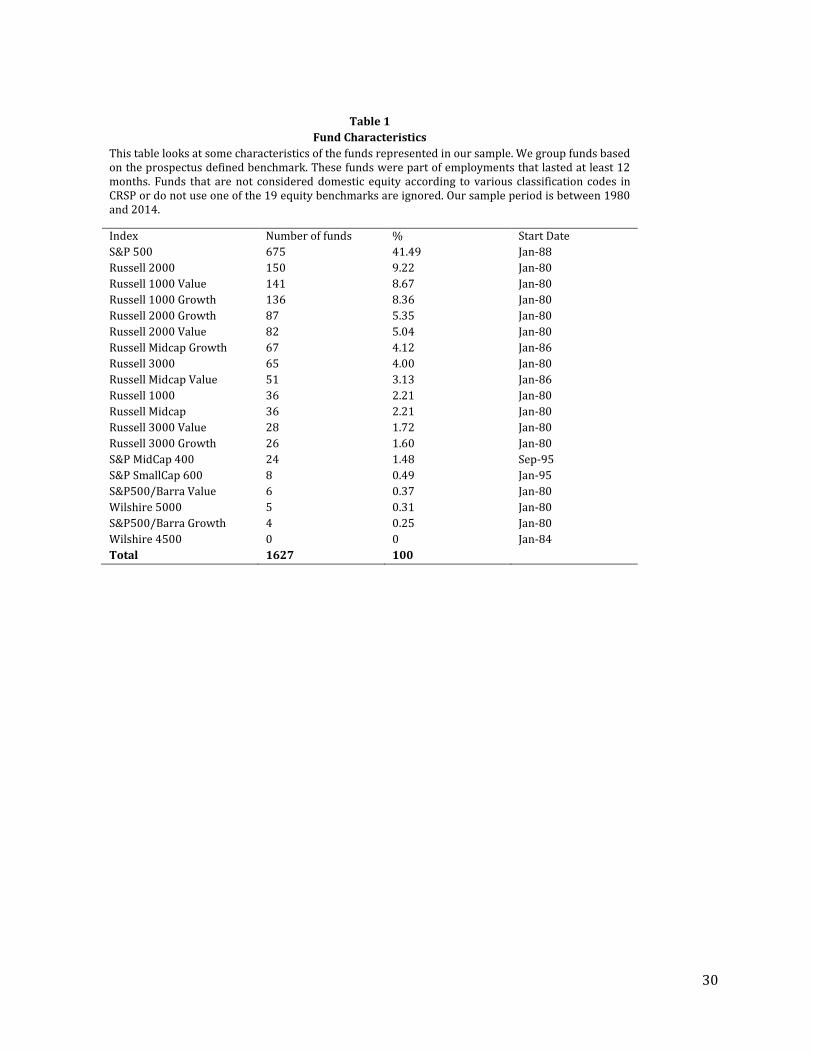
Our sample includes 1,627 distinct mutual funds. According to Table 1, most funds in
our sample use the S&P 500 (41.49%) as a benchmark, followed by Russell 2000 (9.22%),
Russell 1000 Value (8.67%), and Russell 1000 Growth (8.36%). 11 . Overall, our sample
includes funds from all the major equity caps and styles. Most indexes in our study start
reporting in 1980. However, some indexes such as the S&P MidCap 400 and S&P SmallCap
600 start reporting in 1995. Sensoy (2009) uses a sample of 1,815 actively managed,
diversified domestic equity mutual funds from Morningstar that use one of 12 benchmarks,
all of which we include in our study. His sample period is 1994–2004. Of the funds in their
sample, 44.4% use the S& P500, 13.3% use the Russell 2000, 5.9% use the Russell 1000
Growth, and 5.6% use the Russell 1000 Value. Our sample has fewer funds likely because we
require that the fund has employment history data available and that it has at least one
employment that lasts at least 12 months. Also, we require funds to have returns in CRSP
10This is the same list used by Cremers and Petajisto (2009). 11 While we include the Wilshire 4500 as in Cremers and Petajisto (2009), once we screen for employment changes none of the remaining funds in our sample use it as their benchmark.

13
and we identify funds using classification codes in CRSP while Sensoy (2009) uses returns
and fund classifications from Morningstar.
D. Identifying Employments
We create an employment identifier that changes anytime a manager drops or adds a
fund. When the employment identifier changes for a given manager, we create a one year
window pre- and post-employment change. We require all employments to last at least 12
months in order to ensure that we have a long enough sample to accurately measure fund
level constraints but short enough time period that we are not biasing our results to
survivors.12 We end up with 3,537 employment changes. In some cases, there is a gap from
when a manager terminates current employment and transitions to a new employment. One
of the ways in which managers have a gap between employments in our sample is when
managers change employment from equity to non-equity funds. In such cases, they exit our
sample but come back later when they re-enter the equity mutual fund market. As an
additional robustness check, we evaluate employments for which managers may not re-
enter after leaving domestic equity. For the no-gap sample, we have 2,223 employment
changes. We run our main tests using the sample of employment changes with gaps allowed;
however, we also use the sample with no-gaps for robustness.
According to Panel A of Table 2, the average number of employment changes per
manager is 2.96 with a standard deviation of 1.29. We have 1,803 managers that have more
than one employment, while the majority of managers in our sample, 3,361, only have a
single employment. In total we have 5,164 managers represented in our sample. In Panel B,
12 In unreported tables we rerun our analyses across both shorter and longer time periods pre- and post-
employment change and find qualitatively similar results.

14
the length of employments for managers that have a single employment is 66.68 months. For
managers with multiple employments, the average length of each of their employments is
42.56 months. To compute the career length of managers, we assume the career of the
manager started when they entered our sample. To provide an intuitive understanding of
the rate at which managers change employments, we divide the number of employment
changes per manager by the length of the career for each manager in months. In Panel C, we
see that those managers with the longest careers (top quintile) change employment on
average every 8.91 years. While managers with the shortest career (bottom quintile) change
employment on average every 1.7 years.
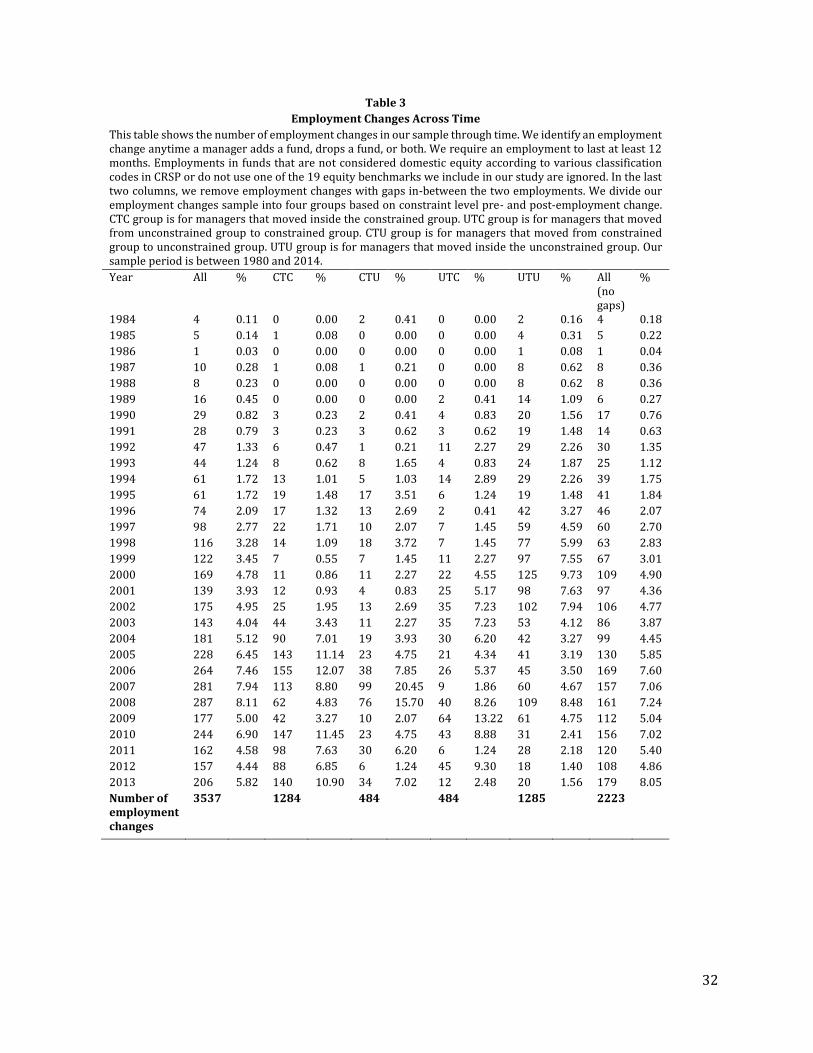
In Table 3, we look at the number of employment changes over time. Consistent with
the large growth in number of funds over our sample period, we find increased fund hiring
over time. There is a noticeable spike in the number of employment changes around the
financial crisis (2007-2008), which is expected as managers are likely laid-off or shift their
portfolios to better match the market demand. For example, during volatile markets we often
see flight to quality. Managers likely leave equity funds for money market funds to better
meet the demand of investors.
Although our time period of our study covers 1980 through 2014, we only report
employment changes from 1984 through 2013 because our first and last employment
change happen in 1984and 2013, respectively. The average number of employment changes
per year for our entire sample (excluding employments with gaps) is 118 and the standard
deviation is 90.8.
E. Key Variables
Constraint

15
We use tracking error as our proxy for fund constraint. Tracking error is calculated
as the standard deviation of the difference between fund returns (Rfund,t) and fund's
benchmark index returns (Rindex,t) over time:
Tracking error = Stdev[Rfund,t− Rindex,t]
As an example, the manager of an S&P 500 index fund is obligated to mimic the S&P 500
index with very little room to deviate from it in search for mispriced securities (high-
constraints create low-tracking error). An aggressive growth fund that allows the manager
discretion to select any stock in the Russell 1000 allows more opportunities for the manager
to deviate from the benchmark in search of mispriced securities (low-constraints create
high-tracking error).
There are two alternate ways which, on face value, could measure constraints.
Cremers and Petajist (2009) measure tracking error as the standard deviation of the residual
from the index model, capturing only idiosyncratic deviation from benchmark returns.
However, limiting managers ability to take systematic risk is a constraint investors could
place on managers. Additionally, one could propose using the R2 from the index model to
measure constraints. This method suffers from the same problem as the residual standard
deviation, capturing only idiosyncratic deviation from the benchmark. Our measure of
tracking error captures both systematic and idiosyncratic constraints placed on fund
managers.
Another method of measuring activism is Active Share, which focuses on deviation
from index holdings (Cremers and Petajisto, 2009). Although Active Share helps better
capture different dimensions of activism, the data requirement of calculating Active Share
(quarterly holdings data) drastically shrinks our sample. Almazan et al. (2004) use mutual

16
fund SEC filings (N-SAR) to measure financial constraints of mutual funds. However, financial
constraints are only one dimension of constraints on mutual fund managers.
The first step to computing employment-level tracking error is to compute an
employment-level returns net of benchmark returns by taking the value-weighted average
of returns net of benchmark returns using monthly TNA for all the funds in the same
employment each month. Second, we take the time-series standard deviation of
employment-level returns net benchmark returns over 12 months pre- and post-
employment change and this is employment-level tracking error pre- and post-employment
change, respectively. The difference between employment-level tracking error pre- and
post-employment change is our main dependent variable, diff_tracking.
For some of our tests we divide employment changes based on the constraint level of
pre- and post-employment change. For each employment change, we use pre- and post-
employment change tracking error windows as our proxy for constraint. We rank all pre-
employment change tracking error windows into constrained (low tracking error or high
constraint) and unconstrained (high tracking error or low constraint) groups based on the
median pre-employment tracking error window. We do the same procedure for the post-
employment change tracking error windows. We classify employments into four groups:
employment changes that resulted in a manager moving within unconstrained group (UTU);
within constrained group (CTC); from unconstrained to constrained employment (UTC); and
from constrained to unconstrained employment (CTU).
Performance
To compute employment-level returns, we first risk-adjust monthly fund returns by
ranking the returns into quintiles each month against their peers in the same benchmark

17
group. We then take the value-weighted average of the ranked returns across funds in the
same employment each month using monthly TNA. 13 Our key independent variable is
returns and is defined as the geometric mean of the employment-level ranked returns for the
12 months pre-employment change. diff_returns is the difference between the geometric
mean of the ranked returns pre- and post-employment using a 12 month window.
Size
To compute an employment-level monthly TNA, we sum the TNA of the funds based
on the employment identifier to get monthly employment-level values. The difference
between pre- and post-employment change average of monthly employment-level TNA over
12 month windows is diff_mtna.
IV. Results
A. Returns and Constraint after an Employment Change
In Table 4 we report the results of change in manager constraint and returns when
an employment change takes place. Change is calculated as the post-employment value
minus the pre-employment value. We evaluate changes in returns and constraint pre- and
post-employment change in order to determine broadly whether manager characteristics
are affected by employment change. We proxy for constraint using the change in 12 month
tracking error measured across net benchmark returns. Panel A reports results based on the
sample that allows gaps in manager employments, and Panel B reports results when
employment gaps are not allowed.
13 In untabulated results, we equal-weight returns and find qualitatively similar results.

18
The first three rows of each panel in Table 4 report results of differences in means of
benchmark ranked returns (diff_returns), raw returns (diff_returns_raw), and tracking error
(diff_tracking)pre-and post-employment change. The fourth through sixth rows of each
panel report the results of differences of the absolute values of means of benchmark ranked
returns, raw returns, and tracking error pre-and post-employment change. We find that the
change in benchmark ranked returns and raw returns of the manager is insignificant
following an employment change; however the constraint level of a manager does change.
When a manager alters their employment (from a more constrained to less constrained or
vice versa) the post-employment change constraint decreases on average. Rows four
through six show that the absolute value of benchmark ranked returns and raw returns does
change when a manager changes employment. This, when interpreted in conjunction with
the results from the first three columns, may imply that when managers underperform they
underperform by more after a change in employment and that when they over perform pre-
employment change they over perform by more post-employment change, but that they
cancel each other out. For robustness, we show the same test using the employment change
sample with no-gaps. Our results do not change.
B. Skill Signal and Hiring Decisions
In Table 5, we evaluate the relationship between performance and future constraints
in order to examine whether over performing managers transition to less constrained
employments, while underperforming managers transition to more constrained
employments. The motivation lies in the belief that if a manager feels over-employed, he or
she will attempt to hide his or her skill level by moving to a more constrained fund in the
future where skill signal is more noisy, while a manager who feels under-employed will

19
attempt to showcase his or her skill in the future by moving to less constrained fund where
skill signal is less noisy.
To empirically evaluate this prediction we regress change in tracking error
(diff_tracking) on past benchmark ranked returns at every employment change. In Panel A
we include all employment changes and in Panel B we include only employments that have
no gaps. Model 1 regresses change in tracking error on pre-employment ranked returns. In
order to remove the effects that growth in assets arise from outperformance (Berk and
Green, 2004) we include the control variable for change in total net assets in Model 2. Models
3 and 4 additionally include year and manager fixed effects respectively. We use year fixed
affects to control for changes in trends as well as trends in the availability of data and
manager fixed effects to control for unobservable manager characteristics.
The results across all four models (across both Panel A and Panel B) show that there
is a statistically significant relationship between pre-employment change returns and pre-
to post- employment change tracking error. The relationship is positive, implying that, on
average, when a manager outperforms relative to peers he or she will transition to lower
constraint employment and when they underperform relative to peers they will transition
to more constrained employments. This follows our theory that managers will self-select
into constraint areas that showcase or hide their skill based on how well they have
performed in the past. Additionally, change in total net assets shows up across all models as
negative and significant. This is as is expected given Berk and Green (2004); as a firm's (or
manager's) assets under management increases they are forced to engage in less activism.
C. Nosiness of Skill Signal

20
In Panels C and D of Table 5, we evaluate whether a manager's skill signal is less noisy
in unconstrained funds than constrained funds. In constrained funds, information
asymmetry gets in the way of observing skill of managers, making it difficult to detect and
reward talent of managers. We predict that managers in unconstrained funds will have a
better gauge of their skill than managers in constrained funds and so we should find that the
relationship between skill and constraint level in hiring is much stronger. However, we
should find that managers in constrained funds are less aware of their skill than managers
in unconstrained funds because of higher information asymmetry and so the relationship
between skill and constraint level in hiring is weaker.
This is what we find in Panels D and C of Table 5. We break employment changes into
two groups; unconstrained (low tracking error) and constrained (high tracking error)
groups based on pre-employment change tracking error over 12 months. We find that for
managers that change employment from constrained employments, the relationship
between returns prior to employment change and change in tracking error is not significant.
However, for managers in the unconstrained employments, we find that relationship
between returns prior to employment change and change in tracking error is significantly
positive.
In Table 6 we examine whether higher returns are required to leave constrained
funds to unconstrained funds because of the noisy signal of returns compared to returns to
remain in unconstrained group. We have speculated that over performance needs to be
higher for managers in constrained funds because the market treats their performance as
being affected by higher information asymmetry. To test this idea we reduce our sample of
employment changes to only those where the managers go from constrained funds to

21
unconstrained funds and those that stay in unconstrained funds. We run logistic regressions
to develop an intuitive understanding of how the probability of a move changes given your
pre-employment change performance.
Panel A of Table 6 shows results from the logistic regressions on the sample that
allows employment gaps and Panel B eliminates employments changes that have gaps.
Model 1, of each panel, is the basic logistic regression of the binary dependent variable of
moving from unconstrained to constrained (binary=1) and unconstrained to unconstrained
(binary=0) on the continuous variable of benchmark ranked returns (returns). Model 2
includes year fixed affects to control for changes in trends as well as trends in the availability
of data.
The results from both Panel A and B of Table 6, as well as Models 1 and 2 show that a
manager is significantly more likely to move from a constrained fund to an unconstrained
fund when the pre-employment change returns are higher than otherwise.
D. Cash Flow Sensitivity
Up to this point, we have examined the return signal only in the context of
employment changes. However, if the noisiness of the signal is driving our results we should
expect to see consistent evidence return signal noisiness outside of hiring. Fund investors
rely on return signals when allocating capital (Berk and Green, 2004; Sirri and Tufano, 1998).
If constrained fund returns are noisier signals of skill we should expect their cash flows to
be less sensitive to performance.
Table 7 reports the results of regressing annual fund net cash flows on the prior year’s
performance. Model (1) reports results without tracking error. As in Sirri and Tufano (1998),
we find an asymmetric relation between flows and performance. Performance, when in the

22
20th percentile or lower (LowRank), has a statistically significant but economically small
0.3057 relation with flows. That relation increases in magnitude for middle performance
(20th through 80th percentile, MidRank) to 0.4058. When funds have returns in the 80th or
higher percentile (HighRank) the relation increases to 1.7011. While the funds in our sample
are punished for poor performance, they are proportionally more greatly rewarded for high
performance.
That relationship changes substantially when we add in tracking error. For easier
interpretation of results, we rank tracking error into deciles annually across all equity funds.
Model (2) includes ranked tracking error both as an independent variable and interacted
with the three performance rank variables. There are three important results from including
tracking error. First, for funds with middle performance (MidRank), flow sensitivity
increases with tracking error. A highly constrained fund, with a tracking error rank of 0, has
a relatively small 0.2549 flow to performance relation. That coefficient increases by 0.0342
for each tracking error rank increase, meaning the least constrained funds (rank 9) have a
0.5627 flow to performance relation. This suggests investors find high constraint fund
returns less informative, just as funds themselves do when hiring.
The second important result out of Model (2) is that high constraint funds have flows
that are more sensitive to extreme performance than low constraint funds. The highest
constrained funds have a flow performance relation of 0.9494 (2.4505) to low (high)
performance, which declines by -0.1237 (-0.1351) for each increase in tracking error rank.
In the extreme, the lowest constrained funds have a flow performance relation of -0.1639 to
low performance and 1.2346 to high performance. It may appear counter intuitive for high
constraint funds to have flows more sensitive to performance. However, this is in fact
23
consistent with a noisier return signal. The only way for a noisy signal to convey information
is for it to be strong. The coefficient on MidRank, representing normal returns (the middle
60% of ranked returns), reveals that on average flows to high constraint funds are less
sensitive to performance. When returns become large enough in absolute terms to clear the
noise (LowRank and HighRank, the top and bottom 20%) investors are responsive to the
signal.
The third important result out of Model (2) is that the traditional asymmetric flow
performance sensitivity found in the literature appears to not be true for high constraint
funds. The highest constraint funds see greater sensitivity to returns when they are low
(LowRank coefficient of 0.9494) than when they are in the middle (MidRank coefficient of
0.2549). The accepted position in the mutual fund literature has long been that funds are
rewarded for high performance with inflows, but see small or zero outflows following poor
performance (see e.g., Chevalier and Ellison, 1997). This appears to only be true for low
constraint funds.
Overall, we interpret these cash flow sensitivity results as consistent with the returns
of high constraint funds being a noisier signal of managerial skill than the returns of low
constraint funds.
V. Conclusion
The role of information asymmetry in the market for agents is difficult to measure but
vital for understanding and mitigating agency costs. We use the market for mutual fund
managers as a natural laboratory for examining the effect signal noise has on the quality of
the hiring process. Returns are an important, but noisy, signal of fund manager ability. The

24
noisiness of that signal is also dependent on the constraints placed on managers, either by
their funds or by themselves. We exploit this cross-sectional dispersion in signal noise to
examine the role of past performance in hiring.
We find that while past performance is an important factor in the manager hiring
decision, past returns appear to only matter when earned at funds with low constraints. In
fact, managers at high constraint funds have to substantially outperform managers at low
constraint funds to be hired by low constraint funds. Additionally, we find that investors are,
on average, more sensitive to returns of low constraint funds than high constraint funds
when allocating capital. This suggests both funds and their investors find the skill signal
present in returns to be noisy. Overall, these findings suggest a misallocation of manager
skill, resulting in skilled managers not moving to funds which need skill and unskilled
managers not being fired when they underperform.

25
References
Akerlof, G. A., 1970, The Market for" Lemons": Quality Uncertainty and the Market
Mechanism. The Quarterly Journal of Economics, 84(3), pp.488-500.
Almazan, A., Brown, K. C., Carlson, M., & Chapman, D. A., 2004, Why Constrain Your Mutual
Fund Manager?, Journal of Financial Economics, 73(2), 289–321.
Avery, C. N., & Chevalier, J. A., 1999, Herding Over the Career, Economic Letters 53, 327-333.
Barras, L., Scaillet, O., & Wermers, R., 2010, False Discoveries in Mutual Fund Performance,
The Journal of Finance 65, 179-216.
Beatty, R., Lu, H., & Luo, W., 2014, The Market for Lemons: A Study of Quality Uncertainty and
the Market Mechanism for Chinese Firms Listed in the US, Working Paper, University
of Southern California.
Berk, J. B., & Green, R. C., 2004, Mutual Fund Flows and Performance in Rational Markets,
Journal of Political Economy, 112(6), 1269-1295.
Bond, E. W., 1982, A Direct Test of the “Lemons” Model: The Market for Used Pickup Trucks,
The American Economic Review 72, 836-840.
Brown, K.C., Harlow, W.V., & Starks L.T., 1996, Of Tournaments and Temptations: An Analysis
of Managerial Incentives in the Mutual Fund Industry, The Journal of Finance 51, 85-
110.
Carlin, Ian, B., & Gervais, S., 2014, Work Ethic, Employment Contracts, and Firm Value, The
Journal of Finance 64, 785-821.
26
Chan, L. K. C., Chen, H., & Lakonishok, J., 2002, On Mutual Fund Investment Styles, Review of
Financial Studies 15, 1407-1437.
Chen, H., Desai, H., & Krishnamurthy, S., 2013, A First Look at Mutual Funds that use Short
Sales, Journal of Financial and Quantitative Analysis 48, 761-787.
Chevalier, J., Ellison, G., 1997, Risk Taking by Mutual Funds as a Response to Incentives,
Journal of Political Economy 105, 1167–1200.
Chevalier, J., Ellison, G., 1999, Career Concerns of Mutual Fund Managers, The Quarterly
Journal of Economics 114, no. 2 (1999): 389-432.
Cremers, M., Ferreira, M. A., Matos, P., and Starks, L., 2016, The Mutual Fund Industry
Worldwide: Explicit and Closet Indexing, Fees, and Performance, forthcoming Journal
of Financial Economics.
Cremers, K. M., & Petajisto, A., 2009, How Active is Your Fund Manager? A New Measure That
Predicts Performance. Review of Financial Studies, hhp057.
Deuskar, P., Pollet, J.M., Wang, J., & Zheng, L., 2011, The Good or the Bad? Which Mutual Fund
Managers Join Hedge Funds?, Review of Financial Studies 24, 3008-3024.
Downing, C., Jaffee, D., & Wallace, N., 2009, Is the Market for Mortgage-Backed Securities a
Market for Lemons?, Review of Financial Studies 22, 2457-2494.
Edelen, R. M., 1999, Investor Flows and the Assessed Performance of Open-End Mutual
Funds, Journal of Financial Economics 53, 439-466.
Elton, E. J., Gruber, M. J., & Blake, C. R., 2012, Does Mutual Fund Size Matter? The Relationship
Between Size and Performance, Review of Asset Pricing Studies 2, 31-55.

27
Eshraghi, A., & Taffler, R., 2012, Fund Manager Overconfidence and Investment Performance:
Evidence from Mutual Funds, Working paper.
Fabel, O., & Lehmann, E., 2000, Adverse Selection and the Economic Limits of Market
Substitution, Working Paper, University of Konstanz.
Fama, E. F., 1980, Agency Problems and the Theory of the Firm, Journal of Political Economy
88, 288-307.
Fama , E. F., & French, K. R., 2010, Luck versus Skill in the Cross-Section of Mutual Fund
Returns, The Journal of Finance 65, 1915-1947.
Fang, J., Kempf, A., & Trapp, M., 2014, Fund Manager Allocation, Journal of Financial
Economics 111, 661-674.
Genesove, D., 1993, Adverse Selection in the Wholesale Used Car Market, Journal of Political
Economy 101, 644-665.
Gibbons, R., and Katz, L. F., 1991, Layoffs and Lemons, Journal of Labor Economics 9, 351-380.
Greenwald B., & Glasspigel, R., 1983, Adverse Selection in the Market for Slaves: New Orleans
1830-1860, Quarterly Journal of Economics 98, 479-499.
Harris, M., & Raviv, A., 1979, Optimal Incentive Contracts with Imperfect Information, Journal
of Economic Theory 20, 231-259.
Holmstrom, B., 1979, Moral Hazard and Observability, The Bell Journal of Economics 10, 74-
91.
Hong, H., Kubik, J. D., & Solomon, A., 2000, Security Analyst’s Career Concerns and Herding
of Earnings Forecasts, RAND Journal of Economics 31, 121-144.
Jensen, M. C., & Meckling, W. H., 1976, Theory of the Firm: Managerial Behavior, Agency Costs
and Ownership Structure, Journal of Financial Economics 3, 305-360.

28
Jensen, M. C., & Murphy, K. J., 1990, Performance Pay and Top-Management Incentives,
Journal of Political Economy 98, 225-264.
Kacperczyk, M., Sialm, C., and Zheng, L., 2008, Unobserved Actions of Mutual Funds, Review
of Financial Studies 21, 2379-2416.
Khorana, A., 1996, Top Management Turnover: An Empirical Investigation of Mutual Fund
Managers, Journal of Financial Economics 40, 403-427.
Kosowski, R., Timmerman, A., Wermers, R., & White, H., 2006, Can Mutual Fund “Starts”
Really Pick Stocks? New Evidence from a Bootstrap Analysis, The Journal of Finance
61, 2551-2595.
Lakonishok, J., Shleifer, A., Thaler, R.H., & Vishny, R., 1991, Window Dressing by Pension Fund
Managers, The American Economic Review 81, 227-231.
Lamont, O., 2002, Macroeconomic Forecasts and Microeconomic Forecasters, Journal of
Economic Behavior and Organization 48, 265-280.
Lehn, K., 1984, Information Asymmetries in Baseball’s Free Agent Market, Economic Inquiry
22, 37-44.
Pan, Y., Wang, T. Y., & Weisbach, M. S., 2015, Learning about CEO Ability and Stock Return
Volatility, Review of Financial Studies28, 1623-1666.
Puetz, A., & Ruenzi, S., 2011, Overconfidence among Professional Investors: Evidence from
Mutual Fund Managers, Journal of Business Finance and Accounting 38, 684-712.
Renneboog, Luc, Jenke Ter Hosrt, and Chendi Zhang, 20011, Is ethical money financially
smart?, Journal of Financial Intermediation 20, 562-588.

29
Rosenman, R .E. & Wilson, W.W., 1991, Quality Differentials and Prices: are Cherries Lemons?
The Journal of Industrial Economics, pp.649-658.
Ross, S.A., 1973, The Economic Theory of Agency: The Principal's Problem. The American
Economic Review, 63(2), pp.134-139.
Sensoy, B.A., 2009, Performance Evaluation and Self-Designated Benchmark Indexes in the
Mutual Fund Industry. Journal of Financial Economics, 92(1), pp.25-39.
Sirri, E. R., & Tufano, P., 1998, Costly Search and Mutual Fund Flows. The Journal of Finance,
53(5), 1589-1622.
Spence, M., 1973, Job Market Signaling, The Quarterly Journal of Economics 87, 355-374.
Stoughton, N. M., 1993, Moral Hazard and the Portfolio Management Problem, The Journal of
Finance, 48(5), pp.2009-2028.
30
Table 1
Fund Characteristics
This table looks at some characteristics of the funds represented in our sample. We group funds based on the prospectus defined benchmark. These funds were part of employments that lasted at least 12 months. Funds that are not considered domestic equity according to various classification codes in CRSP or do not use one of the 19 equity benchmarks are ignored. Our sample period is between 1980 and 2014.
Index Number of funds % Start Date
S&P 500 675 41.49 Jan-88
Russell 2000 150 9.22 Jan-80
Russell 1000 Value 141 8.67 Jan-80
Russell 1000 Growth 136 8.36 Jan-80
Russell 2000 Growth 87 5.35 Jan-80
Russell 2000 Value 82 5.04 Jan-80
Russell Midcap Growth 67 4.12 Jan-86
Russell 3000 65 4.00 Jan-80
Russell Midcap Value 51 3.13 Jan-86
Russell 1000 36 2.21 Jan-80
Russell Midcap 36 2.21 Jan-80
Russell 3000 Value 28 1.72 Jan-80
Russell 3000 Growth 26 1.60 Jan-80
S&P MidCap 400 24 1.48 Sep-95
S&P SmallCap 600 8 0.49 Jan-95
S&P500/Barra Value 6 0.37 Jan-80
Wilshire 5000 5 0.31 Jan-80
S&P500/Barra Growth 4 0.25 Jan-80
Wilshire 4500 0 0 Jan-84
Total 1627 100

31
Table 2
Descriptive Statistics for Employments
This table shows basic statistics about employments of managers in our sample. Number of employment changes is calculated by counting the number of times a manager adds or drops a fund, or both to their portfolio of funds. We require an employment to last at least 12 months. Employments in funds that are not considered domestic equity according to various classification codes in CRSP or do not use one of the 19 equity benchmarks we include in our study are ignored. Length of employment is calculated by counting the number of months since the new employment began until a change of employment. Career length rank is calculated by counting the number of months in the career of each manager and ranking into quantiles. Number of years before an employment change is calculated by dividing the length of the career of the manager in months by the number of employment changes and multiplying by 12. Our sample period is between 1980 and 2014.
Panel A: Number of employment changes throughout the career of managers
Key variable: Number of employment changes per manager
Single employment indicator
N Mean StdDev Minimum Maximum
0 1803 2.96 1.29 2 10
1 3361 1 0 1 1
Number of Managers
5164
Panel B: Number of years at each employment
Key variable: Length of each employment (months)
Single employment Indicator
N Mean StdDev Minimum Maximum
0 5340 42.56 32.74 12 239
1 3361 66.68 52.88 12 244
Total number of employments
8701
Panel C: Number of employment changes and length of career for each manager
Key variable: Number of years before an employment change
Career length rank
N Mean StdDev Minimum Maximum
Shortest Career
1027 1.70 0.45 1.00 2.50
2 1039 3.12 0.84 1.13 4.50
3 1027 4.61 1.73 1.21 7.25
4 1041 6.22 2.99 1.43 11.50
Longest Career
1030 8.91 5.42 1.74 20.33
Number of Managers
5164
32
Table 3
Employment Changes Across Time
This table shows the number of employment changes in our sample through time. We identify an employment change anytime a manager adds a fund, drops a fund, or both. We require an employment to last at least 12 months. Employments in funds that are not considered domestic equity according to various classification codes in CRSP or do not use one of the 19 equity benchmarks we include in our study are ignored. In the last two columns, we remove employment changes with gaps in-between the two employments. We divide our employment changes sample into four groups based on constraint level pre- and post-employment change. CTC group is for managers that moved inside the constrained group. UTC group is for managers that moved from unconstrained group to constrained group. CTU group is for managers that moved from constrained group to unconstrained group. UTU group is for managers that moved inside the unconstrained group. Our sample period is between 1980 and 2014.
Year All % CTC % CTU % UTC % UTU % All (no gaps)
%
1984 4 0.11 0 0.00 2 0.41 0 0.00 2 0.16 4 0.18
1985 5 0.14 1 0.08 0 0.00 0 0.00 4 0.31 5 0.22
1986 1 0.03 0 0.00 0 0.00 0 0.00 1 0.08 1 0.04
1987 10 0.28 1 0.08 1 0.21 0 0.00 8 0.62 8 0.36
1988 8 0.23 0 0.00 0 0.00 0 0.00 8 0.62 8 0.36
1989 16 0.45 0 0.00 0 0.00 2 0.41 14 1.09 6 0.27
1990 29 0.82 3 0.23 2 0.41 4 0.83 20 1.56 17 0.76
1991 28 0.79 3 0.23 3 0.62 3 0.62 19 1.48 14 0.63
1992 47 1.33 6 0.47 1 0.21 11 2.27 29 2.26 30 1.35
1993 44 1.24 8 0.62 8 1.65 4 0.83 24 1.87 25 1.12
1994 61 1.72 13 1.01 5 1.03 14 2.89 29 2.26 39 1.75
1995 61 1.72 19 1.48 17 3.51 6 1.24 19 1.48 41 1.84
1996 74 2.09 17 1.32 13 2.69 2 0.41 42 3.27 46 2.07
1997 98 2.77 22 1.71 10 2.07 7 1.45 59 4.59 60 2.70
1998 116 3.28 14 1.09 18 3.72 7 1.45 77 5.99 63 2.83
1999 122 3.45 7 0.55 7 1.45 11 2.27 97 7.55 67 3.01
2000 169 4.78 11 0.86 11 2.27 22 4.55 125 9.73 109 4.90
2001 139 3.93 12 0.93 4 0.83 25 5.17 98 7.63 97 4.36
2002 175 4.95 25 1.95 13 2.69 35 7.23 102 7.94 106 4.77
2003 143 4.04 44 3.43 11 2.27 35 7.23 53 4.12 86 3.87
2004 181 5.12 90 7.01 19 3.93 30 6.20 42 3.27 99 4.45
2005 228 6.45 143 11.14 23 4.75 21 4.34 41 3.19 130 5.85
2006 264 7.46 155 12.07 38 7.85 26 5.37 45 3.50 169 7.60
2007 281 7.94 113 8.80 99 20.45 9 1.86 60 4.67 157 7.06
2008 287 8.11 62 4.83 76 15.70 40 8.26 109 8.48 161 7.24
2009 177 5.00 42 3.27 10 2.07 64 13.22 61 4.75 112 5.04
2010 244 6.90 147 11.45 23 4.75 43 8.88 31 2.41 156 7.02
2011 162 4.58 98 7.63 30 6.20 6 1.24 28 2.18 120 5.40
2012 157 4.44 88 6.85 6 1.24 45 9.30 18 1.40 108 4.86
2013 206 5.82 140 10.90 34 7.02 12 2.48 20 1.56 179 8.05
Number of employment changes
3537 1284 484 484 1285 2223

33
Table 4
Returns and Constraint Post-Employment Change
This tables looks at how employment-level returns and tracking error change after a change in employment. We require an employment to last at least 12 months. Employments in funds that are not considered domestic equity according to various classification codes in CRSP or do not use one of the 19 equity benchmarks we include in our study are ignored. We risk-adjust fund-level returns by grouping returns based on their prospective defined benchmarks and ranking them against their peers each month. We take the value-weighted average using monthly total net assets of the ranked returns each month in case a manager is managing more than one fund at one point in time to get employment-level risk-adjusted ranked returns for each manager monthly. diff_returns is calculated for each employment change by taking the difference between geometric mean of the pre- and post-employment change employment-level ranked returns using 12 month window. Return variables followed by "raw" indicate that the employment returns have not been risk adjusted. Tracking error is calculated by taking the standard deviation of fund returns less benchmark returns every month. In case of multiple employments, we value-weight the fund returns less benchmark returns to obtain employment-level values. We then take the standard deviation of the employment-level returns net of benchmark returns. diff_tracking is the difference between post-and pre-employment change tracking error using 12 month window. Variables proceeded by "abs" signify that we took the absolute value. For this analysis we ignored managers with a single employment because there is no employment change. For Panel B, we remove employment changes with gaps in-between the two employments. Number of employment changes is calculated by counting the number of times a manager adds or drops a fund, or both to their portfolio of funds. Our sample period is between 1980 and 2014. *, **, *** signify that the mean is significantly different from zero at 10%, 5% and 1% respectively
Panel A: Employments with gaps allowed
Variable Number of employment changes Mean StdDev
diff_returns 3537 0.0025 0.6081
diff_returns_raw 3537 -0.0003 0.0255
diff_tracking 3537 -0.0017*** 0.0133
abs_diff_returns 3537 0.4746*** 0.3802
abs_diff_returns_raw 3537 0.0184*** 0.0177
abs_diff_tracking 3537 0.00781*** 0.0109
Panel B: Employments with gaps not allowed
diff_returns 2223 -0.0093 0.5941
diff_returns_raw 2223 -0.0007 0.0245
diff_tracking 2223 -0.0013*** 0.0102
abs_diff_returns 2223 0.4597*** 0.3763
abs_diff_returns_raw 2223 0.0170*** 0.0176
abs_diff_tracking 2223 0.0064*** 0.0080

34
Table 5
Skill Signal and Hiring Decisions
We regress the change of tracking error after an employment change on returns pre-employment change. We identify an employment change anytime a manager adds a fund, drops a fund, or both. We require an employment to last at least 12 months. Employments in funds that are not considered domestic equity according to various classification codes in CRSP or do not use one of the 19 equity benchmarks we include in our study are ignored. We risk-adjust fund-level returns by grouping returns based on their prospectus defined benchmarks and ranking them against their peers each month. We take the value-weighted average of the ranked returns each month using monthly total net assets (mtna) in case a manager is managing more than one fund at one point in time to get employment-level ranked returns for each manager monthly. returns is calculated for each manager by taking the geometric mean of the pre-employment change employment-level ranked returns using 12 month window. Tracking error is calculated by taking the standard deviation of fund returns less benchmark returns each month. In case of multiple employments, we value-weight the returns less benchmark returns to obtain employment-level values. We then take the standard deviation of the employment-level returns net of benchmark returns. diff_tracking is the difference between post-and pre-employment change tracking error using 12 month window. diff_mtna is calculated by first summing the mtna of all funds under same employment every month in case of multiple funds in a single employment. We then take the difference between the average of mtna pre- and post-employment change using 12 month window. For this analysis we ignored managers with a single employment because there is no employment change. For panel B, we remove employment changes with gaps in-between the two employments. In panel C and D, we divide our original employment changes sample into two groups; constrained and unconstrained employments based on the median of the tracking error pre-employment change using 12 month window. We then run the same regression as in panel A. Our sample period is between 1980 and 2014. *, **, *** signify significance at 10%, 5% and 1%, respectively
Panel A: Employment gaps allowed Panel B: Employment gaps not allowed
DV diff_tracking diff_tracking diff_tracking diff_tracking diff_tracking diff_tracking diff_tracking diff_tracking
(1) (2) (3) (4) (1) (2) (3) (4)
Intercept -0.0097 -0.010 -0.0083 -0.0083
returns 0.0029*** 0.0030*** 0.0031*** 0.0034*** 0.0026*** 0.0026*** 0.0027*** 0.0027***
diff_mtna (x106) -0.1019*** -0.0958*** -0.0952*** -0.0439** -0.0341* -0.0675**
AdjR-Sq 0.0096 0.0147 0.1349 0.5712 0.0123 0.0139 0.1665 0.6051
Year FE 0 0 1 0 0 0 1 0
Manager FE 0 0 0 1 0 0 0 1
N 3537 3537 3537 3537 2223 2223 2223 2223
Panel C: Constrained group (CTU and CTC) Panel D: Unconstrained group (UTC and UTU)
DV diff_tracking diff_tracking diff_tracking diff_tracking diff_tracking diff_tracking diff_tracking diff_tracking
(1) (2) (3) (4) (1) (2) (3) (4)
Intercept 0.0027 0.003 -0.0137 -0.0139
returns -0.0002 -0.0002 -0.0004 0.0009 0.0031*** 0.0032*** 0.0041*** 0.0044***
diff_mtna(x106) -0.0437*** -0.0286** -0.0253*** -0.3012*** -0.3197*** -0.2422*
AdjR-Sq -0.0003 0.0059 0.1277 0.7034 0.0075 0.0186 0.1409 0.6409
Year FE 0 0 1 0 0 0 1 0
Manager FE 0 0 0 1 0 0 0 1
N 1768 1768 1768 1768 1769 1769 1769 1769

35
Table 6
Noisiness of Skill Signal
This table shows the results from our logistic regression. We look for employment changes where the manager moved from constrained group to the unconstrained group (CTU) or remained in the unconstrained group (UTU). We rank employments based on tracking error pre- and post- employment change using 12 month window. We identify an employment change anytime a manager adds a fund, drops a fund, or both. We require an employment to last at least 12 months. Employments in funds that are not considered domestic equity according to various classification codes in CRSP or do not use one of the 19 equity benchmarks we include in our study are ignored. We risk-adjust fund-level returns by grouping returns based on their prospectus defined benchmarks and ranking them against their peers each month. We take the value-weighted average of the ranked returns each month using monthly total net assets (mtna) in case a manager is managing more than one fund at one point in time to get employment-level ranked returns for each employment monthly. returns is calculated for each manager by taking the geometric mean of the pre-employment change employment-level ranked returns using 12 month window. Tracking error is calculated by taking the standard deviation of fund returns less benchmark returns each month. In case of multiple employments, we value-weight the returns less benchmark returns to obtain employment-level values. We then take the standard deviation of the employment-level returns net of benchmark returns. diff_tracking is the difference between post-and pre-employment change tracking error using 12 month window. diff_mtna is calculated by first summing the mtna of all funds under management every month in case of multiple funds. We then take the difference between the average of mtna pre- and post-employment change using 12 month window. For this analysis we ignored managers with single employment because there is no employment change. For panel B, we remove employment changes with gaps in-between the two employments. Our sample period is between 1980 and 2014. *, **, *** signify significance at 10%, 5% and 1%, respectively
Panel A: Employment gaps allowed Panel B: Employment gaps not allowed
DV 1=CTU 0=UTU
1=CTU 0=UTU
1=CTU 0=UTU
1=CTU 0=UTU
(1) (2) (1) (2)
Intercept -1.832 -4.0433 -2.0244 -5.2820
returns 0.3141*** 0.4794*** 0.3136** 0.6113***
diff_mtna (x106) -20.0000** -20.0000* -20.0000* -20.0000***
Year FE 0 1 0 1
N (CTU) 484 484 266 266
N(UTU) 1285 1285 846 846
N 1769 1769 1022 1022
Wald (Pr>ChiSq) 0.0011 <.0001 0.0155 <.0001

36
Table 7
Cash Flow Sensitivity
This table shows the results from annual net cash flows regressed on fund characteristics and performance. Flows in year t are defined as (TNAt – (1+Rett)TNAt-1) / TNAt-1. Objective flow is TNA-weighted mean flows in year t of all funds in the same investment objective, grouped into Growth, Growth and Income, Small Capitalization, and Aggressive Growth by Lipper Objective Code. TNA, Expense Ratios, and Loads are as reported in CRSP. Max Load is the largest of the front and rear loads. Return Stdev is the annual standard deviation of monthly returns. Tracking Error is the tracking error of monthly fund returns (as defined in Table 4) over the 12 months of year t. Returns are ranked into percentiles annually by investment objective and converted into three piece-wise variables as in Sirri and Tufano (1998). LowRank is returns in the lowest 20th percentile, MidRank is returns between the 20th and 80th percentiles, and HighRank is returns in the 80th percentile. Regression use pooled OLS with standard errors clustered by year. T-statistics are reported in parentheses. Our sample period is between 1980 and 2012.
Model (1) Model (2)
Intercept 0.4670 6.56 0.4031 4.33
Log(TNAt-1) -0.0719 -11.12 -0.0737 -11.04
Objective Flowt 1.1362 14.02 1.1963 15.41
Expense Ratiot-1 2.9927 1.21 1.7640 0.69
Max Loadt-1 -0.2349 -0.87 -0.0754 -0.27
Return Stdevt-1 -0.5578 -1.09 -0.4553 -0.81
Tracking Errort-1 0.0147 1.71
LowRank t-1 0.3057 2.16 0.9494 3.21
MidRank t-1 0.4058 6.26 0.2549 3.59
HighRank t-1 1.7011 4.38 2.4505 4.41
LowRank t-1*TE t-1 -0.1237 -2.69
MidRank t-1*TE t-1 0.0342 3.02
HighRank t-1*TE t-1 -0.1351 -1.59
N 19,258 18,698
R2 0.1095 0.1099
Related Documents


![Reputation & Regulations: Evidence from eBay1 Introduction Asymmetric information can lead to adverse selection, moral hazard, market ine ciency, or even market failure (Akerlof[1970]).](https://static.cupdf.com/doc/110x72/5fde385cd2ccbd0951181025/reputation-regulations-evidence-from-1-introduction-asymmetric-information.jpg)


