Lecture Three Chapters Two and three Photo slides from Digital Image Processing, Gonzalez and Woods, Copyright 2002.

Lecture Three

Chapters Two and threePhoto slides from Digital Image Processing, Gonzalez and Woods, Copyright 2002

Chapter 2: Digital Image FundamentalsChapter 2: Digital Image Fundamentals

Functional Represenation of Images

• Two-D function f(x,y), (x,y) pixel position. Postive and bounded

• Written as f(x,y)=i(x,y)r(x,y), i(x,y) illumination from light source, r(x,y) reflectance (bounded between 0 and 1) based on material properties. E.g r(x,y)=0.01 for black velvet, r(x,y) = 0.93 for snow.

• Intensity of monochrome image f(x,y) is synonymous with grey levels. By convention grey level are from 0 to L-1.



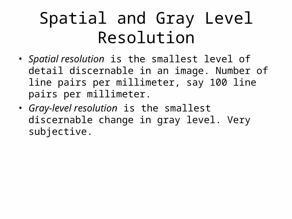
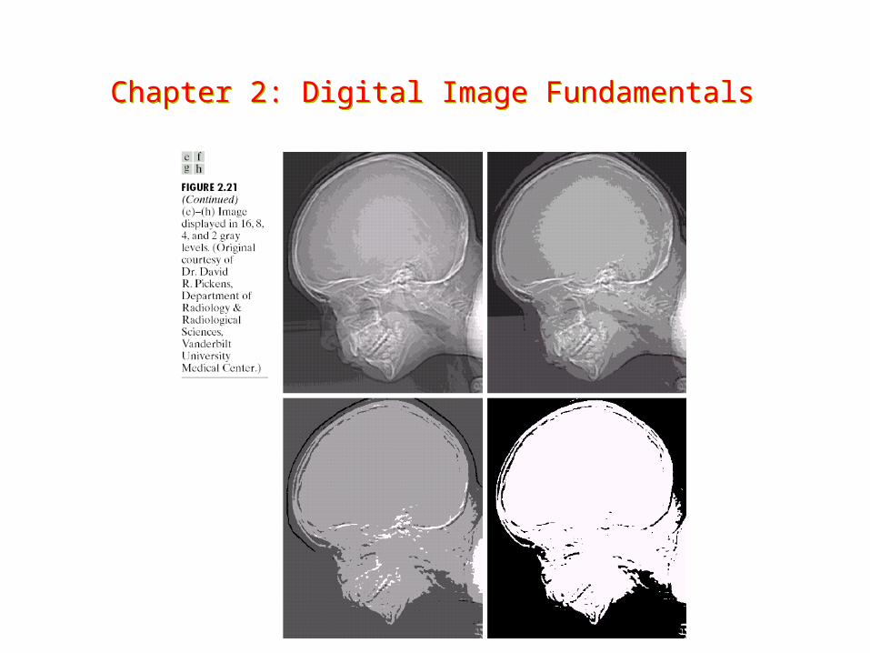
Spatial and Gray Level Resolution

• Spatial resolution is the smallest level of detail discernable in an image. Number of line pairs per millimeter, say 100 line pairs per millimeter.

• Gray-level resolution is the smallest discernable change in gray level. Very subjective.




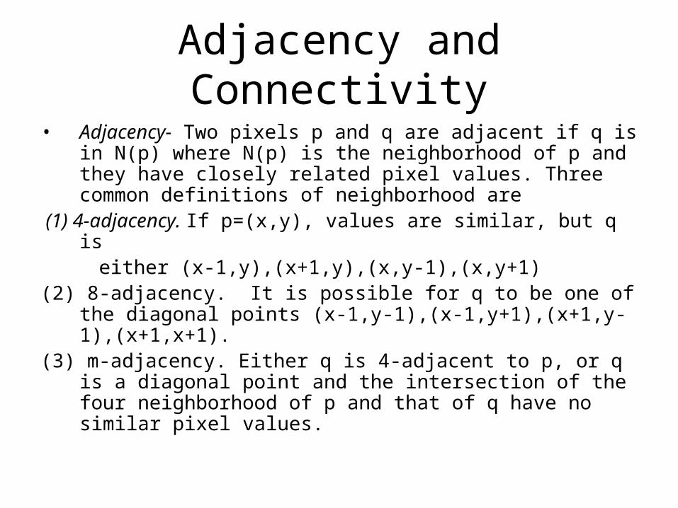
Adjacency and Connectivity

• Adjacency- Two pixels p and q are adjacent if q is in N(p) where N(p) is the neighborhood of p and they have closely related pixel values. Three common definitions of neighborhood are

(1) 4-adjacency. If p=(x,y), values are similar, but q is either (x-1,y),(x+1,y),(x,y-1),(x,y+1)(2) 8-adjacency. It is possible for q to be one of the

diagonal points (x-1,y-1),(x-1,y+1),(x+1,y-1),(x+1,x+1).(3) m-adjacency. Either q is 4-adjacent to p, or q is a

diagonal point and the intersection of the four neighborhood of p and that of q have no similar pixel values.

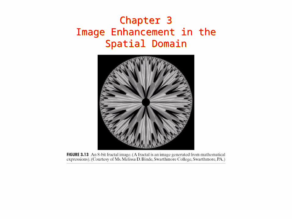
Chapter 3Image Enhancement in the

Spatial Domain


Spatial Domain


Adjacency ,More Formally

Choose a set of gray values V. If f(p) and

f(q) are in V, and q is in the right kind of neighborhood of p, then p and q are adjacent.

I can model this relationship using 0-1 images, why??

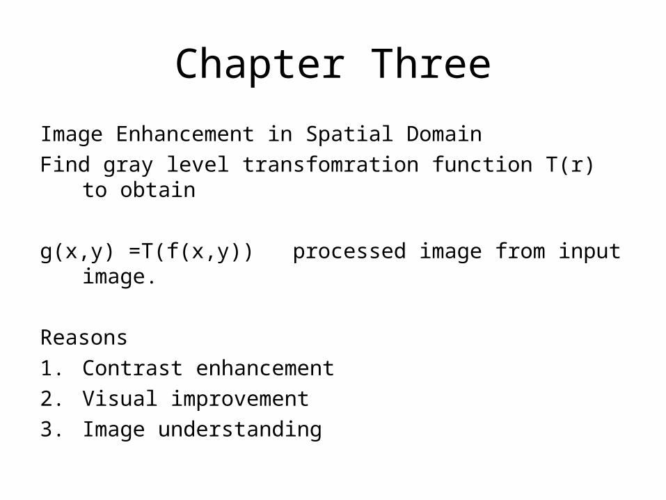
Chapter Three

Image Enhancement in Spatial Domain

Find gray level transfomration function T(r) to obtain

g(x,y) =T(f(x,y)) processed image from input image.

Reasons

1. Contrast enhancement

2. Visual improvement

3. Image understanding


Spatial Domain


Spatial Domain

Negatives

Here

T(r) = L-1-r L-1 maximum gray level

Produces photographic negative. Some details are easier to spot if we go from black and white to white and black.


Spatial Domain


Spatial Domain

Mammogram

Notice that the white or gray detail in the dark region is more visible in the negative.

This shows a small lesion.


Spatial Domain


Spatial Domain

Log Transformation

T(r) = c log(1+s)

Inverse Log

T(r) = exp(r/c)-1

For the next picture, c=1. Used to display Fourier spectra.


Spatial Domain


Spatial Domain

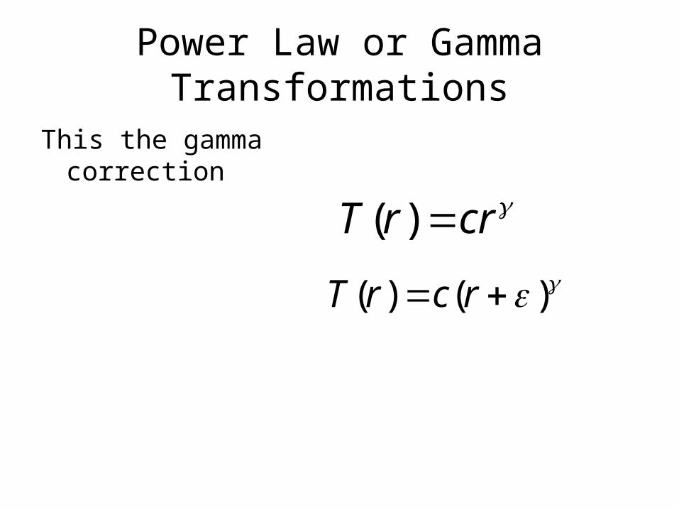
Power Law or Gamma Transformations

This the gamma correction

crrT )( )()( rcrT


Spatial Domain


Spatial Domain

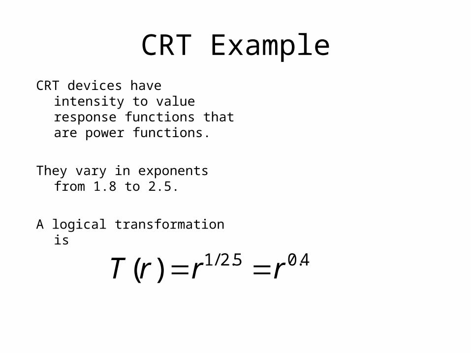
CRT ExampleCRT devices have intensity to

value response functions that are power functions.

They vary in exponents from 1.8 to 2.5.

A logical transformation is

4.05.2/1)( rrrT


Spatial Domain


Spatial Domain

MRI of Fractured Spine

Transformation is

With gamma = 0.6,0.4,0.3

rrT )(


Spatial Domain


Spatial Domain


Spatial Domain


Spatial Domain


Spatial Domain


Spatial Domain


Spatial Domain


Spatial Domain


Spatial Domain


Spatial Domain


Spatial Domain


Spatial Domain


Spatial Domain


Spatial Domain

Lecture Three Chapters Two and three Photo slides from Digital Image Processing, Gonzalez and Woods, Copyright 2002.

Documents

y processed image

input image

digital image processing

y illumination

y reflectance

y pixel position

thespatial domainchapter

chapter threeimage enhancement