Lecture Notes on Undergraduate Physics Kevin Zhou [email protected] These notes review the undergraduate physics curriculum, with an emphasis on quantum mechanics. They cover, essentially, the material that every working physicist should know. The notes assume everything in the high school Physics Olympiad syllabus as prerequisite knowledge. Nothing in these notes is original; they have been compiled from a variety of sources. The primary sources were: • David Tong’s Classical Dynamics lecture notes. A friendly set of notes that covers Lagrangian and Hamiltonian mechanics with neat applications, such as the gauge theory of a falling cat. • Arnold, Mathematical Methods of Classical Mechanics. The classic advanced mechanics book. The first half of the book covers Lagrangian mechanics compactly, with nice and tricky problems, while the second half covers Hamiltonian mechanics geometrically. • David Tong’s Electrodynamics lecture notes. Covers electromagnetism at the standard Griffiths level. Especially nice because it does the most complex calculations in index notation, when vector notation becomes clunky or ambiguous. • David Tong’s Statistical Mechanics lecture notes. Has an especially good discussion of phase transitions, which leads in well to a further course on statistical field theory. • Blundell and Blundell, Concepts in Thermal Physics. A good first statistical mechanics book filled with applications, touching on information theory, non-equilibrium thermodynamics, the Earth’s atmosphere, and much more. • David Tong’s Applications of Quantum Mechanics lecture notes. A conversational set of notes, with a focus on solid state physics. Also contains a nice section on quantum foundations. • Robert Littlejon’s Physics 221 notes. An exceptionally clear set of graduate-level quantum mechanics notes, with a focus on atomic physics: you read it and immediately understand. Every important point and pitfall is discussed carefully, and complex material is developed elegantly, often in a cleaner and more rigorous way than in any of the standard textbooks. Much of these notes are just an imperfect summary of Littlejon’s notes; most diagrams are his. The most recent version is here; please report any errors found to [email protected].

Welcome message from author
This document is posted to help you gain knowledge. Please leave a comment to let me know what you think about it! Share it to your friends and learn new things together.
Transcript

Lecture Notes on
Undergraduate PhysicsKevin Zhou
These notes review the undergraduate physics curriculum, with an emphasis on quantum mechanics.
They cover, essentially, the material that every working physicist should know. The notes assume
everything in the high school Physics Olympiad syllabus as prerequisite knowledge. Nothing in
these notes is original; they have been compiled from a variety of sources. The primary sources
were:
• David Tong’s Classical Dynamics lecture notes. A friendly set of notes that covers Lagrangian
and Hamiltonian mechanics with neat applications, such as the gauge theory of a falling cat.
• Arnold, Mathematical Methods of Classical Mechanics. The classic advanced mechanics book.
The first half of the book covers Lagrangian mechanics compactly, with nice and tricky problems,
while the second half covers Hamiltonian mechanics geometrically.
• David Tong’s Electrodynamics lecture notes. Covers electromagnetism at the standard Griffiths
level. Especially nice because it does the most complex calculations in index notation, when
vector notation becomes clunky or ambiguous.
• David Tong’s Statistical Mechanics lecture notes. Has an especially good discussion of phase
transitions, which leads in well to a further course on statistical field theory.
• Blundell and Blundell, Concepts in Thermal Physics. A good first statistical mechanics book
filled with applications, touching on information theory, non-equilibrium thermodynamics, the
Earth’s atmosphere, and much more.
• David Tong’s Applications of Quantum Mechanics lecture notes. A conversational set of notes,
with a focus on solid state physics. Also contains a nice section on quantum foundations.
• Robert Littlejon’s Physics 221 notes. An exceptionally clear set of graduate-level quantum
mechanics notes, with a focus on atomic physics: you read it and immediately understand.
Every important point and pitfall is discussed carefully, and complex material is developed
elegantly, often in a cleaner and more rigorous way than in any of the standard textbooks.
Much of these notes are just an imperfect summary of Littlejon’s notes; most diagrams are his.
The most recent version is here; please report any errors found to [email protected].

Contents
1 Classical Mechanics 1
1.1 Lagrangian Formalism . . . . . . . . . . . . . . . . . . . . . . . . . . . . . . . . . . . 1
1.2 Rigid Body Motion . . . . . . . . . . . . . . . . . . . . . . . . . . . . . . . . . . . . . 4
1.3 Hamiltonian Formalism . . . . . . . . . . . . . . . . . . . . . . . . . . . . . . . . . . 8
1.4 Poisson Brackets . . . . . . . . . . . . . . . . . . . . . . . . . . . . . . . . . . . . . . 10
1.5 Action-Angle Variables . . . . . . . . . . . . . . . . . . . . . . . . . . . . . . . . . . . 14
1.6 The Hamilton–Jacobi Equation . . . . . . . . . . . . . . . . . . . . . . . . . . . . . . 17
2 Electromagnetism 21
2.1 Electrostatics . . . . . . . . . . . . . . . . . . . . . . . . . . . . . . . . . . . . . . . . 21
2.2 Magnetostatics . . . . . . . . . . . . . . . . . . . . . . . . . . . . . . . . . . . . . . . 23
2.3 Electrodynamics . . . . . . . . . . . . . . . . . . . . . . . . . . . . . . . . . . . . . . 26
2.4 Relativity . . . . . . . . . . . . . . . . . . . . . . . . . . . . . . . . . . . . . . . . . . 29
2.5 Radiation . . . . . . . . . . . . . . . . . . . . . . . . . . . . . . . . . . . . . . . . . . 32
2.6 Electromagnetism in Matter . . . . . . . . . . . . . . . . . . . . . . . . . . . . . . . . 39
3 Statistical Mechanics 46
3.1 Ensembles . . . . . . . . . . . . . . . . . . . . . . . . . . . . . . . . . . . . . . . . . . 46
3.2 Thermodynamics . . . . . . . . . . . . . . . . . . . . . . . . . . . . . . . . . . . . . . 52
3.3 Entropy and Information . . . . . . . . . . . . . . . . . . . . . . . . . . . . . . . . . 57
3.4 Classical Gases . . . . . . . . . . . . . . . . . . . . . . . . . . . . . . . . . . . . . . . 59
3.5 Bose–Einstein Statistics . . . . . . . . . . . . . . . . . . . . . . . . . . . . . . . . . . 64
3.6 Fermi–Dirac Statistics . . . . . . . . . . . . . . . . . . . . . . . . . . . . . . . . . . . 70
4 Kinetic Theory 76
4.1 Fundamentals . . . . . . . . . . . . . . . . . . . . . . . . . . . . . . . . . . . . . . . . 76
4.2 The Boltzmann Equation . . . . . . . . . . . . . . . . . . . . . . . . . . . . . . . . . 79
4.3 Hydrodynamics . . . . . . . . . . . . . . . . . . . . . . . . . . . . . . . . . . . . . . . 83
5 Fluids 84
6 Fundamentals of Quantum Mechanics 85
6.1 Physical Postulates . . . . . . . . . . . . . . . . . . . . . . . . . . . . . . . . . . . . . 85
6.2 Wave Mechanics . . . . . . . . . . . . . . . . . . . . . . . . . . . . . . . . . . . . . . 90
6.3 The Adiabatic Theorem . . . . . . . . . . . . . . . . . . . . . . . . . . . . . . . . . . 93
6.4 Particles in Electromagnetic Fields . . . . . . . . . . . . . . . . . . . . . . . . . . . . 97
6.5 The Harmonic Oscillator . . . . . . . . . . . . . . . . . . . . . . . . . . . . . . . . . . 101
6.6 Coherent States . . . . . . . . . . . . . . . . . . . . . . . . . . . . . . . . . . . . . . . 103
6.7 The WKB Approximation . . . . . . . . . . . . . . . . . . . . . . . . . . . . . . . . . 107
7 Path Integrals 113
7.1 Formulation . . . . . . . . . . . . . . . . . . . . . . . . . . . . . . . . . . . . . . . . . 113
7.2 Gaussian Integrals . . . . . . . . . . . . . . . . . . . . . . . . . . . . . . . . . . . . . 115
7.3 Semiclassical Approximation . . . . . . . . . . . . . . . . . . . . . . . . . . . . . . . 117
8 Angular Momentum 122
8.1 Classical Rotations . . . . . . . . . . . . . . . . . . . . . . . . . . . . . . . . . . . . . 122
8.2 Representations of su(2) . . . . . . . . . . . . . . . . . . . . . . . . . . . . . . . . . . 124
8.3 Spin and Orbital Angular Momentum . . . . . . . . . . . . . . . . . . . . . . . . . . 129
8.4 Central Force Motion . . . . . . . . . . . . . . . . . . . . . . . . . . . . . . . . . . . . 133
8.5 Addition of Angular Momentum . . . . . . . . . . . . . . . . . . . . . . . . . . . . . 140
8.6 Tensor Operators . . . . . . . . . . . . . . . . . . . . . . . . . . . . . . . . . . . . . . 143
9 Discrete Symmetries 148
9.1 Parity . . . . . . . . . . . . . . . . . . . . . . . . . . . . . . . . . . . . . . . . . . . . 148
9.2 Time Reversal . . . . . . . . . . . . . . . . . . . . . . . . . . . . . . . . . . . . . . . . 150
10 Time Independent Perturbation Theory 155
10.1 Formalism . . . . . . . . . . . . . . . . . . . . . . . . . . . . . . . . . . . . . . . . . . 155
10.2 The Stark Effect . . . . . . . . . . . . . . . . . . . . . . . . . . . . . . . . . . . . . . 158
10.3 Fine Structure . . . . . . . . . . . . . . . . . . . . . . . . . . . . . . . . . . . . . . . 162
10.4 The Zeeman Effect . . . . . . . . . . . . . . . . . . . . . . . . . . . . . . . . . . . . . 168
10.5 Hyperfine Structure . . . . . . . . . . . . . . . . . . . . . . . . . . . . . . . . . . . . 172
10.6 The Variational Method . . . . . . . . . . . . . . . . . . . . . . . . . . . . . . . . . . 176
11 Atomic Physics 180
11.1 Identical Particles . . . . . . . . . . . . . . . . . . . . . . . . . . . . . . . . . . . . . 180
11.2 Helium . . . . . . . . . . . . . . . . . . . . . . . . . . . . . . . . . . . . . . . . . . . . 183
11.3 The Thomas–Fermi Model . . . . . . . . . . . . . . . . . . . . . . . . . . . . . . . . . 189
11.4 The Hartree–Fock Method . . . . . . . . . . . . . . . . . . . . . . . . . . . . . . . . . 192
11.5 Atomic Structure . . . . . . . . . . . . . . . . . . . . . . . . . . . . . . . . . . . . . . 197
11.6 Chemistry . . . . . . . . . . . . . . . . . . . . . . . . . . . . . . . . . . . . . . . . . . 201
12 Time Dependent Perturbation Theory 202
12.1 Interaction Picture . . . . . . . . . . . . . . . . . . . . . . . . . . . . . . . . . . . . . 202
12.2 Fermi’s Golden Rule . . . . . . . . . . . . . . . . . . . . . . . . . . . . . . . . . . . . 204
12.3 The Born Approximation . . . . . . . . . . . . . . . . . . . . . . . . . . . . . . . . . 206
12.4 Atoms in Fields . . . . . . . . . . . . . . . . . . . . . . . . . . . . . . . . . . . . . . . 208
13 Scattering 212
13.1 Introduction . . . . . . . . . . . . . . . . . . . . . . . . . . . . . . . . . . . . . . . . . 212
13.2 Partial Waves . . . . . . . . . . . . . . . . . . . . . . . . . . . . . . . . . . . . . . . . 214
13.3 Green’s Functions . . . . . . . . . . . . . . . . . . . . . . . . . . . . . . . . . . . . . 218
13.4 The Lippmann–Schwinger Equation . . . . . . . . . . . . . . . . . . . . . . . . . . . 224
13.5 The S-Matrix . . . . . . . . . . . . . . . . . . . . . . . . . . . . . . . . . . . . . . . . 227
1 1. Classical Mechanics
1 Classical Mechanics
1.1 Lagrangian Formalism
We begin by carefully considering generalized coordinates.
• Consider a system with Cartesian coordinates xA. Hamilton’s principle states that solutions
of the equations of motion are critical points of the action S =∫Ldt. Then we have the
Euler–Lagrange equationd
dt
∂L
∂x=∂L
∂x
where we have dropped indices for simplicity. Here, we have L = L(x, x) and the partial
derivative is defined by holding all other arguments of the function constant.
• It follows directly from the chain rule that the Euler–Lagrange equations are preserved by any
invertible coordinate change, to generalized coordinates qa = qa(xA), because the action is a
property of a path and hence is extremized regardless of the coordinates used to describe the
path. The ability to use any generalized coordinates we want is a key practical advantage of
Lagrangian mechanics over Newtonian mechanics.
• It is a little less obvious this holds for time-dependent transformations qa = qa(xA, t), so we
will prove this explicitly. Again dropping indices,
∂L
∂q=∂L
∂x
∂x
∂q+∂L
∂x
∂x
∂q
where we have q = q(x, x, t) and hence by invertibility x = x(q, t) and x = x(q, q, t), and
x =∂x
∂qq +
∂x
∂t.
This yields the ‘cancellation of dots’ identity
∂x
∂q=∂x
∂q.
• As for the other side of the Euler–Lagrange equation, note that
d
dt
∂L
∂q=
d
dt
(∂L
∂x
∂x
∂q
)=∂L
∂x
∂x
∂q+∂L
∂x
d
dt
∂x
∂q
where, in the first step, we used ∂x/∂q = 0 since x is not a function of q, and in the second
step, we used cancellation of dots and the Euler–Lagrange equation.
• To finish the derivation, we note that
d
dt
∂q
∂x=∂q
∂x
which may be shown by direct expansion.
• It is a bit confusing why these partial derivatives are allowed. The point is that we are working
on the tangent bundle of some manifold, where the position and velocity are independent. They
are only related once we evaluate quantities on a specific path x(t). All total time derivatives
here implicitly refer to such a path.

2 1. Classical Mechanics
Next we show that if constraints exist, we can work in a reduced set of generalized coordinates.
• A holonomic constraint is a relationship of the form
fα(xA, t) = 0
which must hold on all physical paths. Holonomic constraints are useful because each one can
be used to eliminate a generalized coordinate; note that inequalities are not holonomic.
• Velocity-dependent constraints are holonomic if they can be ‘integrated’. For example, consider
a ball rolling without slipping. In one dimension, this is holonomic, since v = Rθ. In two
dimensions, it’s possible to roll the ball in a loop and have it come back in a different orientation.
Formally, a velocity constraint is holonomic if there is no nontrivial holonomy.
• To find the equations of motion, we use the Lagrangian
L′ = L(xA, xA) + λαfα(xA, t).
We think of the λα as additional, independent coordinates; then the Euler–Lagrange equation
∂L′/∂λα = 0 reproduces the constraint. The Euler–Lagrange equations for the xA now have
constraint forces equal to the Lagrange multipliers.
• Now we switch coordinates from xA, λα to qa, fα, λα, continuing to use the Lagrangian L′. The
Euler–Lagrange equations are simply
d
dt
∂L
∂qa− ∂L
∂qi=
∂
∂qaλαfα = 0, λα = fα = 0.
Thus, in these generalized coordinates, the constraint forces have disappeared. We may restrict
to the coordinates qa and use the original Lagrangian L. Note that in such an approach, we
cannot solve for the values of the constraint forces.
• In problems with symmetry, there will be conserved quantities, which may be formally written
as constraints on the positions and velocities. However, it’s important to remember that they
are not genuine constraints, because they only hold on-shell. Treating a conserved quantity as
a constraint and using the procedure above will give incorrect results.
• We may think of the coordinates qa as contravariant under changes of coordinates. Then the
conjugate momenta are covariant, so the quantity piqi is invariant. Similarly, the differential
form pidqi is invariant.
• We say a Lagrangian is regular if
det∂2L
∂qi∂qj6= 0.
In this case, the equation of motion can be solved for q. We’ll mostly deal with regular
Lagrangians, but irregular ones can appear in relativistic particle mechanics.
Example. Purely kinetic Lagrangians. In the case
L =1
2gab(qc)q
aqb
3 1. Classical Mechanics
the equation of motion is the geodesic equation
qa + Γabcqbqc = 0, Γabc =
1
2gad (∂cgbd + ∂bgcd − ∂dgbc)
where we have assumed the metric is invertible, and symmetrized the geodesic coefficients. This
works just like the derivation in general relativity, except that in that context, the metric and
velocities include a time component, so the solutions have stationary proper time.
Example. A particle in an electromagnetic field. The Lagrangian is
L =1
2mr2 − e(φ− r ·A).
With a little index manipulation, this reproduces the Lorentz force law, with
B = ∇×A, E = −∇φ− ∂A
∂t.
The momentum conjugate to r is
p =∂L
∂r= mr + eA
and is called the canonical momentum, in contrast to the kinetic momentum mr. The canonical
momentum is what becomes the gradient operator in quantum mechanics, but it is not gauge
invariant; instead the kinetic momentum is. The switch from partial to covariant derivatives in
gauge theory is analogous to the switch from canonical to kinetic momentum.
Example. A single relativistic particle. The Lagrangian should be a Lorentz scalar, and the only
one available is the proper time. Setting c = 1, we have
L = −m√
1− r2
Then the momentum is γmv as expected, and the action is proportional to the proper time,
S = −m∫ √
dt2 − dr2 = −m∫dτ.
Now consider how one might add a potential term. For a nonrelativistic particle, the potential term
is additive; in the relativistic case it can go inside or outside the square root. The two options are
S1 = −m∫ √(
1 +2V
m
)dt2 − dr2, S2 = −m
∫dτ +
∫V dt.
Neither of these options are Lorentz invariant, which makes sense if we regard V as sourced by a
fixed background. However, we can get a Lorentz invariant action if we also transform the source.
In both cases, we need to extend V to a larger object. In the first case we must promote V to a
rank 2 tensor (because dt2 is rank 2), while in the second case we must promote V to a four-vector
(because dt is rank 1),
S1 = −m∫ √
gµνdxµdxν , S2 = −m∫dτ + e
∫Aµdx
µ.
These two possibilities yield gravity and electromagnetism, respectively. We see that in the nonrel-
ativistic limit, gµν = ηµν + hµν for small hµν , c2h00/2 becomes the gravitational potential.
4 1. Classical Mechanics
There are a few ways to see this “in advance”. For example, the former forces the effect of
the potential to be proportional to the mass, which corresponds to the equivalence of inertial and
gravitational mass in gravity. Another way to argue this is to note that electric charge is assumed to
be Lorentz invariant; this is experimentally supported because atoms are electrically neutral, despite
the much greater velocities of the electrons. This implies the charge density is the timelike part of
a current four-vector jµ. Since the source of electromagnetism is a four-vector, the fundamental
field Aµ is as well. However, the total mass/energy is not Lorentz invariant, but rather picks up a
factor of γ upon Lorentz transformation. This is because the energy density is part of a tensor Tµν ,
and accordingly the gravitational field in relativity is described by a tensor gµν .
Specializing to electromagnetism, we have
L = −m√
1− r2 − e(φ− r ·A)
where we parametrize the path as r(t). Alternatively, parametrizing it as xµ(τ) as we did above,
the equation of motion is
md2xµ
dτ2= eFµν
dxνdτ
, Fµν = ∂µAν − ∂νAµ
where Fµν is the field strength tensor. The current associated with the particle is
jµ(x) = e
∫dτ
dxµ
dτδ(x− x(τ)).
Further discussion of the relativistic point particle is given in the notes on String Theory.
1.2 Rigid Body Motion
We begin with the kinematics of rigid bodies.
• A rigid body is a collection of masses constrained so that ‖ri − rj‖ is constant for all i and j.
Then a rigid body has six degrees of freedom, from translations and rotations.
• If we fix a point to be the origin, we have only the rotational degrees of freedom. Define a fixed
coordinate system ea as well as a moving body frame ea(t) which moves with the body.
Both sets of axes are orthogonal and thus related by an orthogonal matrix,
ea(t) = Rab(t)eb(t), Rab = ea · eb.
Since the body frame is specified by R(t), the configuration space C of orientations is SO(3).
• Every point r in the body can be expanded in the space frame or the body frame as
r(t) = ra(t)ea = raea(t).
Note that the body frame changes over time as
deadt
=dRabdt
eb =
(dR
dtR−1
)ab
eb
This prompts us to define the matrix ω = RR−1, so that ea = ωabeb.
5 1. Classical Mechanics
• The matrix ω is antisymmetric, so we take the Hodge dual to get the angular velocity vector
ωa =1
2εabcωbc, ω = ωaea.
Inverting this relation, we have ωaεabc = ωbc. Substituting into the above,
deadt
= −εabcωbec = ω× ea
where we used (ea)d = δad.
• The above is just a special case of the formula
v = ω× r
which can be derived from simple vector geometry. Using that picture, the physical interpretation
of ω is n dφ/dt, where n is the instantaneous axis of rotation and dφ/dt is the rate of rotation.
Generally, both n and dφ/dt change with time.
Example. To get an explicit formula for R(t), note that R = ωR. The naive solution is the
exponential, but since ω doesn’t commute with itself at different times, we must use the path
ordered exponential,
R(t) = P exp
(∫ t
0ω(t′)dt′
).
For example, the second-order term here is∫ t′′
0
(∫ t
t′ω(t′′) dt′′
)ω(t′) dt′
where the ω’s are ordered from later to earlier. Then when we differentiate with respect to t, it
only affects the dt′′ integral, which pops out a factor of ω on the left as desired. This exponential
operation relates rotations R in SO(3) with infinitesimal rotations ω in so(3).
We now turn from kinematics to dynamics.
• Using v = ω× r, the kinetic energy is
T =1
2
∑miv
2 =1
2
∑mi‖ω× ri‖2 =
1
2
∑mi
(ω2r2
i − (ri · ω)2).
This implies that
T =1
2ωaIabωb
where Iab is the symmetric tensor
Iab =∑i
mi
(r2i δab − (ri)a(ri)b
)called the inertia tensor. Note that since the components of ω are in the body frame, so are
the components of I and ri that appear above; hence the Iab are constant.
6 1. Classical Mechanics
• Explicitly, for a continuous rigid body with mass density ρ(r), we have
I =
∫d3r ρ(r)
y2 + z2 −xy −xz−xy x2 + z2 −yz−xz −yz x2 + y2
.
• Since I is symmetric, we can rotate the body frame to diagonalize it. The eigenvectors are
called the principal axes and the eigenvalues Ia are the principal moments of inertia. Since T
is nonnegative, I is positive semidefinite, so Ia ≥ 0.
• Parallel axis theorem states that if I0 is the inertia tensor about the center of mass, the inertia
tensor about the point c is
(Ic)ab = (I0)ab +M(c2δab − cacb).
The proof is similar to the two-dimensional parallel axis theorem, with contributions proportional
to∑miri vanishing. The extra contribution the inertia tensor we would get if the object’s
mass was entirely at the center of mass.
• Similarly, the translational and rotational motion of a free spinning body ‘factorize’. If the
center of mass position is R(t), then
T =1
2MR2 +
1
2ωaIabωb.
This means we can indeed ignore the center of mass motion for dynamics.
• The angular momentum is
L =∑
miri × vi =∑
miri × (ω× ri) =∑
mi(r2iω− (ω · ri)ri).
We thus recognize
L = Iω, T =1
2ω · L.
For general I, the angular momentum and angular velocity are not parallel.
• To find the equation of motion, we use dL/dt in the center of mass frame, for
0 =dLadt
ea + Ladeadt
=dLadt
ea + Laω× ea.
Dotting both sides by eb gives 0 = La + εaijωILj . In the case of principle axes (L1 = I1ω1),
I1ω1 + ω2ω3(I3 − I2) = 0
along with cyclic permutations thereof. These are Euler’s equations. In the case of a torque,
the components of the torque (in the principle axis frame) appear on the right.
We now analyze the motion of free tops. We consider the time evolution of the vectors L, ω, and
e3. In the body frame, e3 is constant and points upward; in the space frame, L is constant, and for
convenience we take it to point upward. In general, we know that L and 2T = ω · L are constant.

7 1. Classical Mechanics
Example. A spherical top. In this trivial case, ωa = 0, so ω doesn’t move in the body frame, nor
does L. In the space frame, L and ω are again constant, and the axis e3 rotates about them. As a
simple example, the motion of e3 looks like the motion of a point on the globe as it rotates about
its axis.
Example. The symmetric top. Suppose I1 = I2 6= I3, e.g. for a top with radial symmetry. Then
I1ω1 = ω2ω3(I1 − I3), I2ω2 = −ω1ω3(I1 − I3), I3ω3 = 0.
Then ω3 is constant, while the other two components rotate with frequency
Ω = ω3(I1 − I3)/I1.
This implies that |ω| is constant. Moreover, we see that L, ω, and e3 all lie in the same plane.
In the body frame, both ω and L precess about e3. Similarly, in the space frame, both ω and e3
precess about L. To visualize this motion, consider the point e2 and the case where Ω, ω1, ω2 ω3.
Without the precession, e2 simply rotates about L, tracing out a circle. With the precession, the
orbit of e2 also ‘wobbles’ slightly with frequency Ω.
Example. The Earth is an oblate ellipsoid with (I1− I3)/I1 ≈ −1/300, with ω3 = (1 day)−1. Since
the oblateness itself is caused by the Earth’s rotation, the angular velocity is very nearly aligned
with e3, though not exactly. We thus expect the Earth to wobble with a period of about 300 days;
this phenomenon is called the Chandler wobble.
Example. The asymmetric top. If all of the Ii are unequal, the Euler equations are much more
difficult to solve. Instead, we can consider the effect of small perturbations. Suppose that
ω1 = Ω + η1, ω2 = η2, ω3 = η3.
To first order in η, the Euler equations become
I1η1 = 0, I2η2 = Ωη3(I3 − I1), I3η3 = Ωη2(I1 − I2).
Combining the last two equations, we have
I2η2 =Ω2
I3(I3 − I1)(I1 − I2)η2.
Therefore, we see that rotation about e1 is unstable iff I1 is in between I2 and I3. An asymmetric
top rotates stably only about the principal axes with largest and smallest moment of inertia.
8 1. Classical Mechanics
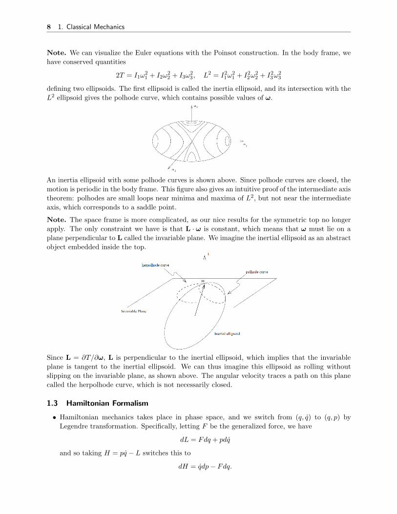
Note. We can visualize the Euler equations with the Poinsot construction. In the body frame, we
have conserved quantities
2T = I1ω21 + I2ω
22 + I3ω
23, L2 = I2
1ω21 + I2
2ω22 + I2
3ω23
defining two ellipsoids. The first ellipsoid is called the inertia ellipsoid, and its intersection with the
L2 ellipsoid gives the polhode curve, which contains possible values of ω.
An inertia ellipsoid with some polhode curves is shown above. Since polhode curves are closed, the
motion is periodic in the body frame. This figure also gives an intuitive proof of the intermediate axis
theorem: polhodes are small loops near minima and maxima of L2, but not near the intermediate
axis, which corresponds to a saddle point.
Note. The space frame is more complicated, as our nice results for the symmetric top no longer
apply. The only constraint we have is that L · ω is constant, which means that ω must lie on a
plane perpendicular to L called the invariable plane. We imagine the inertial ellipsoid as an abstract
object embedded inside the top.
Since L = ∂T/∂ω, L is perpendicular to the inertial ellipsoid, which implies that the invariable
plane is tangent to the inertial ellipsoid. We can thus imagine this ellipsoid as rolling without
slipping on the invariable plane, as shown above. The angular velocity traces a path on this plane
called the herpolhode curve, which is not necessarily closed.
1.3 Hamiltonian Formalism
• Hamiltonian mechanics takes place in phase space, and we switch from (q, q) to (q, p) by
Legendre transformation. Specifically, letting F be the generalized force, we have
dL = Fdq + pdq
and so taking H = pq − L switches this to
dH = qdp− Fdq.

9 1. Classical Mechanics
In the language of thermodynamics, we have L = L(q, q) and H = H(q, p) naturally. In order
to write H in terms of these variables, we must be able to eliminate q in favor of p, which is
generally only possible if L is convex in q.
• Plugging in F = dp/dt, we arrive at Hamilton’s equations,
pi = −∂H∂qi
, qi =∂H
∂pi.
The explicit time dependence just comes along for the ride, giving
dH
dt=∂H
∂t= −∂L
∂t
where the first equality follows from Hamilton’s equations and the chain rule.
• We may also derive Hamilton’s equations by minimizing the action
S =
∫(piqi −H) dt.
In this context, the variations in pi and qi are independent. However, as before, δq = ˙(δq).
Plugging in the variation, we see that δq must vanish at the endpoints to integrate by parts,
while δp doesn’t have to, so our formulation isn’t totally symmetric.
• When L is time-independent with L = T − V , and L is a quadratic homogeneous function in q,
we have pq = 2T , so H = T + V . Then the value of the Hamiltonian is the total energy.
Example. The Hamiltonian for a particle in an electromagnetic field is
H =(p− eA)2
2m− eφ
where p = mr + eA is the canonical momentum. We see that the Hamiltonian is numerically
unchanged by the addition of a magnetic field (since magnetic fields do no work), but the time
evolution is affected, since the canonical momentum is different.
Carrying out the same procedure for our non-covariant relativistic particle Lagrangian gives
H =√m2c2 + c2(p− eA)2 + eφ.
However, doing it for the covariant Lagrangian, with λ as the “time parameter”, yields H = 0. This
occurs generally for reparametrization-invariant actions. The notion of a Hamiltonian is inherently
not Lorentz invariant, as they generate time translation in a particular frame.
Both of the examples above are special cases of the minimal coupling prescription: to incorporate
an interaction with the electromagnetic field, we must replace
pµ → pµ − eAµ
which corresponds, in nonrelativistic notation, to
E → E − eφ, p→ p− eA.
In general, minimal coupling is a good first guess, because it is the simplest Lorentz invariant option.
In field theory, it translates to adding a term∫dx JµAµ where Jµ is the matter 4-current. However,
we would need a non-minimal coupling to account for, e.g. the spin of the particle.
10 1. Classical Mechanics
Hamiltonian mechanics leads to some nice theoretical results.
• Liouville’s theorem states that volumes of regions of phase space are constant. To see this,
consider the infinitesimal time evolution
qi → qi +∂H
∂pidt, pi → pi −
∂H
∂qidt.
Then the Jacobian matrix is
J =
(I + (∂2H/∂pi∂qj)dt (∂2H/∂pi∂pj)dt
−(∂2H/∂qi∂qj)dt I − (∂2H/∂qi∂pj)dt
).
Using the identity det(I + εM) = 1 + ε trM , we have det J = 1 by equality of mixed partials.
• In statistical mechanics, we might have a phase space probability distribution ρ(q, p, t). The
convective derivative dρ/dt is the rate of change while comoving with the phase space flow,
∂ρ
∂t=
∂ρ
∂pi
∂H
∂qi− ∂ρ
∂qi
∂H
∂pi
and Liouville’s theorem implies that dρ/dt = 0.
• Liouville’s theorem holds even if energy isn’t conserved, as in the case of an external field. It
fails in the presence of dissipation, where there isn’t a Hamiltonian description at all.
• Poincare recurrence states that for a system with bounded phase space, given an initial point
p, every neighborhood D0 of p contains a point that will return to D0 in finite time.
Proof: consider the neighborhoods Dk formed by evolving D0 with time kT for an arbitrary
time T . Since the phase space volume is finite, and the Dk all have the same volume, we
must have some overlap between two of them, say Dk and Dk′ . Since Hamiltonian evolution is
reversible, we may evolve backwards, yielding an overlap between D0 and Dk−k′ .
• As a corollary, it can be shown that Hamiltonian evolution is generically either periodic or
fills some submanifold of phase space densely. We will revisit this below in the context of
action-angle variables.
1.4 Poisson Brackets
The formalism of Poisson brackets is closely analogous to quantum mechanics.
• The Poisson bracket of two functions f and g on phase space is
f, g =∑i
∂f
∂qi
∂g
∂pi− ∂f
∂pi
∂g
∂qi.
Geometrically, it is possible to associate g with a vector field Xg, and f, g is the rate of change
of f along the flow of Xg.
• Applying Hamilton’s equations, for any function f(p, q, t),
df
dt= f,H+
∂f
∂t
where the total derivative is a convective derivative; this states that the flow associated with
H is time translation. In particular, if I(p, q) satisfies I,H = 0, then I is conserved.

11 1. Classical Mechanics
• The Poisson bracket is antisymmetric, linear, and obeys the product rule
fg, h = fg, h+ f, hg
as expected from the geometric intuition above. It also satisfies the Jacobi identity, so the space
of functions with the Poisson bracket is a Lie algebra.
• A related property is the “chain rule”. If f = f(hi), then
f, g =∑ ∂f
∂hihi, g.
This can be seen by applying the regular chain rule and the flow idea above.
• By the Jacobi identity, Lie brackets of conserved quantities are also conserved, so conserved
quantities form a Lie subalgebra.
Example. In statistical mechanics, ensembles are time-independent distributions on phase space.
Applying Liouville’s equation, we require ρ,H = 0. If the conserved quantities of a system are fi,
then ρ may be any function of the fi, i.e. any member of the subalgebra of conserved quantities.
We typically take the case where only the energy is conserved for simplicity. In this case, the
microcanonical ensemble is ρ ∝ δ(H − E) and the canonical ensemble is ρ ∝ e−βH .
Example. The Poisson brackets of position and momentum are always zero, except for
qi, pj = δij .
The flow generated by momentum is translation along its direction, and vice versa for position.
Example. Angular momentum. Defining L = r× p, we have
Li, Lj = εijkLk, L2, Li = 0
as in quantum mechanics. The first equation may be understood intuitively from the commutation
of infinitesimal rotations.
We now consider the changes of coordinates that preserve the form of Hamilton’s equations; these are
called canonical transformations. Generally, they are more flexible than coordinate transformations
in the Lagrangian formalism, since we can mix position and momentum.
• Define x = (q1, . . . , qn, p1, . . . , pn)T and define the matrix J as
J =
(0 In−In 0
)Then Hamilton’s equations become
x = J∂H
∂x.
Also note that the canonical Poisson brackets are xi, xj = Jij .

12 1. Classical Mechanics
• Now consider a transformation qi → Qi(q, p) and pi → Pi(q, p), written as xi → yi(x). Then
y = (J JJ T )∂H
∂y
where J is the Jacobian matrix Jij = ∂yi/∂xj . We say the Jacobian is symplectic if J JJ T is
the identity, and in this case, the transformation is called canonical.
• The Poisson bracket is invariant under canonical transformations. To see this, note that
f, gx = (∂xf)TJ(∂xg)
where (∂xf)i = ∂f/∂xi. By the chain rule, ∂x = J T∂y, giving the result. Then if we only
consider canonical transformations, we don’t have to specify which coordinates the Poisson
bracket is taken in.
• Conversely, if a transformation preserves the canonical Poisson brackets yi, yjx = Jij , it is
canonical. To see this, apply the chain rule for
Jij = yi, yjx =(J JJ T
)ij
which is exactly the condition for a canonical transformation.
Example. Consider a ‘point transformation’ qi → Qi(q). We have shown that these leave Lagrange’s
equations invariant, but in the Hamiltonian formalism, we also must transform the momentum
accordingly. Dropping indices and defining Θ = ∂Q/∂q,
J =
(Θ 0
∂P/∂q ∂P/∂p
), J JJ T =
(0 Θ(∂P/∂p)T
−ΘT∂P/∂p 0
)which implies that Pi = (Θ−1
ji )pj , in agreement with the formula Pi = ∂L/∂Qi. Since Θ depends
on q, the momentum P is a function of both p and q.
We now consider infinitesimal canonical transformations.
• Consider a canonical transformation Qi = qi + αFi(q, p) and Pi = pi + αEi(q, p) where α is
small. Expanding the symplectic condition to first order yields
∂Fi∂qj
= −∂Ej∂pi
,∂Fi∂pj
=∂Fj∂pi
,∂Ei∂qj
=∂Ej∂qi
.
There are all automatically satisfied if
Fi =∂G
∂pi, Ei = −∂G
∂qi
for some G(q, p), and we say G generates the transformation.
• More generally, consider a one-parameter family of canonical transformations parametrized by
α. Then by the above,
dqidα
=∂G
∂pi,
dpidα
= −∂G∂qi
,df
dα= f,G.
Interpreting the transformation actively, this looks just like evolution under a Hamiltonian,
with G in place of H and α in place of t. The infinitesimal canonical transformation generated
by G(p, q, α) is flow under its vector field.

13 1. Classical Mechanics
• We say G is a symmetry of H if the flow generated by G does not change H, i.e. H,G = 0.
But this is just the condition for G to be conserved: since the Poisson bracket is antisymmetric,
flow under H doesn’t change G either. This is Noether’s theorem in Hamiltonian mechanics.
• For example, using G = H simply generates time translation, y(t) = x(t − t0). Less trivially,
G = pk generates qi → qi + αδik, so momentum generates translations.
Now we give a very brief glimpse of the geometrical formulation of classical mechanics.
• In Lagrangian mechanics, the configuration space is a manifold M , and the Lagrangian is a
function on its tangent bundle L : TM → R. The action is a real-valued function on paths
through the manifold.
• The momentum p = ∂L/∂q is a covector on M , and we have a map
F : TM → T ∗M, (q, q) 7→ (q,p)
called the Legendre transform, which is invertible if the Lagrangian is regular. The cotangent
bundle T ∗M can hence be identified with phase space.
• A cotangent bundle has a canonical one-form ω = pidqi, where the qi are arbitrary coordinates
and the pi are coordinates in the dual basis. Its exterior derivative Ω = dpi∧dqi is a symplectic
form, i.e. a closed and nondegenerate two-form on an even-dimensional manifold.
• Conversely, the Darboux theorem states that for any symplectic form we may always choose
coordinates so that locally it has the form dpi ∧ dqi.
• The symplectic form relates functions f on phase space to vector fields Xf by
iXfΩ = df, ΩµνX
µf = ∂νf
where iXfis the interior product with Xf , and the indices range over the 2 dimM coordinates
of phase space. The nondegeneracy condition means the form can be inverted, giving
Xµf = Ωµν∂νf
and thus Xf is unique given f .
• Time evolution is flow under XH , so the rate of change of any phase space function f is XH(f).
• The Poisson bracket is defined as
f, g = Ω(Xf , Xg) = Ωµν∂µf∂νg.
The closure of Ω implies the Jacobi identity for the Poisson bracket.
• If flow under the vector field X preserves the symplectic form, LXΩ = 0, then X is called a
Hamiltonian vector field. In particular, using Cartan’s magic formula and the closure of Ω, this
holds for all Xf derived from the symplectic form.
• If Ω is preserved, so is any exterior power of it. Since Ωn is proportional to the volume form,
its conservation recovers Liouville’s theorem.
Note. Consider a single particle with a parametrized path xµ(τ). Then the velocity is naturally a
Lorentz vector and the canonical momentum is a Lorentz covector. However, the physical energy
and momentum are vectors, because they are the conserved quantities associated with translations,
which are vectors. Hence we must pick up signs when converting canonical momentum to physical
momentum, which is the fundamental reason why p = −i∇ but H = +i∂t in quantum mechanics.

14 1. Classical Mechanics
1.5 Action-Angle Variables
The additional flexibility of canonical transformations allows us to use even more convenient variables
than the generalized coordinates of Lagrangian mechanics. Often, the so-called action-angle variables
are a good choice, which drastically simplify the problem.
Example. The simple harmonic oscillator. The Hamiltonian is
H =p2
2m+
1
2mω2q2
and we switch from (q, p) to (θ, I), where
q =
√2I
mωsin θ, p =
√2Imω cos θ.
To confirm this is a canonical transformation, we check that Poisson brackets are preserved; the
simplest way to do this is to work backwards, noting that
q, p(θ,I) = 2√I sin θ,
√I cos θ(θ,I) = 1
as desired. In these new coordinates, the Hamiltonian is simply
H = ωI, θ = ω, I = 0.
We have “straightened out” the phase space flow into straight lines on a cylinder. This is the
simplest example of action angle variables.
• In general, for n degrees of freedom, we would like to find variables (θi, Ii) so that the Hamiltonian
is only a function of the Ii. Then the Ii are conserved, and θi = ωi, where the ωi depend on
the Ii but are time independent. When the system is bounded, we scale θi to lie in [0, 2π). The
resulting variables are called action-angle variables, and the system is integrable.
• Liouville’s theorem states that if there are n mutually Poisson commuting constants of motion
Ii, then the system is integrable. (At first glance, this seems to be a trivial criterion – how
could one possibly prove that such constants of motion don’t exist? However, it is possible; for
instance, Poincare famously proved that there were no such conserved quantities for the general
three body problem, analytic in the canonical variables and the masses.)
• Integrable systems are rare and special; chaotic systems are not integrable. The question of
whether a system is integrable has to do with global structure, since one can always straighten
out the phase space flow lines locally.
• The motion of an integrable system lies on a surface of constant Ii. These surfaces are topolog-
ically tori Tn, called invariant tori.
Example. Action-angle variables for a general one-dimensional system. Let
H =p2
2m+ V (x).
The value of H is the total energy E, so the action variable I must satisfy
θ = ω = dE/dI

15 1. Classical Mechanics
where the period of the motion is 2π/ω. Now, by conservation of energy
dt =
√m
2
dq√E − V (q)
.
Integrating over a single orbit, we have
2π
ω=
√m
2
∮dq√
E − V (q)=
∮ √2m
d
dE
√E − V (q) dq =
d
dE
∮ √2m(E − V (q)) dq =
d
dE
∮p dq.
Note that by pulling the d/dE out of the integral, we neglected the change in phase space area due
to the change in the endpoints of the path, because this contribution is second order in dE.
Therefore, we have the nice results
I =1
2π
∮p dq, T =
d
dE
∮p dq.
We can thus calculate T without finding a closed-form expression for θ, which can be convenient.
For completeness, we can also determine θ, by
θ = ωt =dE
dI
d
dE
∫p dq =
d
dI
∫p dq.
Here the value of θ determines the upper bound on the integral, and the derivative acts on the
integrand.
We now turn to adiabatic invariants.
• Consider a situation where the Hamiltonian depends on a parameter λ(t) that changes slowly.
Then energy is not conserved; taking H(q(t), p(t), λ(t)) = E(t) and differentiating, we have
E =∂H
∂λλ.
However, certain “adiabatic invariants” are approximately conserved.
• We claim that in the case
H =p2
2m+ V (q;λ(t))
the adiabatic invariant is simply the action variable I. Since I is always evaluated on an orbit
of the Hamiltonian at a fixed time, it is only a function of E and λ, so
I =∂I
∂E
∣∣∣∣λ
E +∂I
∂λ
∣∣∣∣E
λ.
These two contributions are due to the nonconservation of energy, and from the change in the
shape of the orbits at fixed energy, respectively.
• When λ is constant, E = E(I) as before, so
∂I
∂E
∣∣∣∣λ
=1
ω(λ)=T (λ)
2π.
16 1. Classical Mechanics
As for the second term, we have
∂I
∂λ
∣∣∣∣E
=1
2π
∮∂p
∂λ
∣∣∣∣E
dq =1
2π
∮∂p
∂λ
∣∣∣∣E
∂H
∂p
∣∣∣∣λ,q
dt′
where we applied Hamilton’s equations, and neglected a higher-order term from the change in
the endpoints.
• To simplify the integrand, take H(q, p(q, λ,E), λ) = E and differentiate with respect to λ at
fixed E. Then∂H
∂q
∣∣∣∣λ,p
∂q
∂λ
∣∣∣∣E
+∂H
∂p
∣∣∣∣λ,q
∂p
∂λ
∣∣∣∣E
+∂H
∂λ
∣∣∣∣q,p,E
= 0.
By construction, the first term is zero. Then we conclude that
∂I
∂λ
∣∣∣∣E
= − 1
2π
∮∂H
∂λ
∣∣∣∣E
dt′.
Finally, combining this with our first result, we conclude
I =
(T (λ)
∂H
∂λ
∣∣∣∣E
−∫∂H
∂λ
∣∣∣∣E
dt′)λ
2π.
Taking the time average of I and noting that the change in λ is slow compared to the period
of the motion, the two quantities above cancel, so 〈I〉 = 0 and I is an adiabatic invariant.
Example. The simple harmonic oscillator has I = E/ω. Then if ω is changed slowly, the ratio
E/ω remains constant. The above example also manifests in quantum mechanics; for example, for
quanta in a harmonic oscillator, we have E = n~ω. If the ω of the oscillator is changed slowly, the
energy can only remain quantized if E/ω remains constant, as it does in classical mechanics.
Example. The adiabatic theorem can also be proved heuristically with Liouville’s theorem. We
consider an ensemble of systems with fixed E but equally spaced phase θ, which thus travel along
a single closed curve in phase space. Under any time variation of λ, the phase space curve formed
by the systems remains closed, and the area inside it is conserved because none can leak in or out.
Now suppose λ is varied extremely slowly. Then every system on the ring should be affected in
the same way, so the final ring remains a curve of constant energy E′. By the above reasoning, the
area inside this curve is conserved, proving the theorem.
Example. A particle in a magnetic field. Consider a particle confined to the xy plane, experiencing
a magnetic field
B = B(x, y, t)z
which is slowly varying. Also assume that B is such that the particle forms closed orbits. If the
variation of the field is slow, then the adiabatic theorem holds. Integrating over a cycle gives
I =1
2π
∮p · dq ∝
∫mv · dq− e
∫A · dq =
2π
ωmv2 − eΦB.
In the case of a uniform magnetic field, we have
v = Rω, ω =eB
m
17 1. Classical Mechanics
which shows that the two terms are proportional; hence the magnetic flux is conserved. Alternatively,
since ΦB = AB and B ∝ ω, the magnetic moment of the current loop made by the particle is
conserved; this is called the first adiabatic invariant by plasma physicists. One consequence is that
charged particles can be heated by increasing the field.
Alternatively, suppose that B = B(r) and the particle performs circular orbits centered about
the origin. Then the adiabatic invariant can be written as
I ∝ r2(2B −Bav)
where Bav is the average field inside the circular orbit. This implies that as B(r, t) changes in time,
the orbit will get larger or smaller unless we have 2B = Bav, a condition which betatron accelerators,
which accelerate particles by changing the magnetic field in this way, are designed to satisfy.
The first adiabatic invariant is also the principle behind magnetic mirrors. Suppose one has a
magnetic field B(x, y, z) where Bz dominates, and varies slowly in space. Particles can perform
helical orbits, spiraling along magnetic field lines. The speed is invariant, so
v2x + v2
y + v2z = const.
On the other hand, if we boost to match the vz of a spiraling particle, then the situation looks just
like a particle in the xy plane with a time-varying magnetic field. Approximating the orbit as small
and the Bz inside as roughly constant, we have
I ∝ mv2
ω∝v2x + v2
y
Bz= const.
Therefore, as Bz increases, vz decreases, and at some point the particle will be “reflected” and spiral
back in the opposite direction. This is the principle behind magnetic mirrors, which can be used to
confine plasmas in fusion reactors.
1.6 The Hamilton–Jacobi Equation
We begin by defining Hamilton’s principal function.
• Given initial conditions (qi, ti) and final conditions (qf , tf ), there can generally be multiple
classical paths between them. Often, paths are discrete, so we may label them with a branch
index b. However, note that for the harmonic oscillator we need a continuous branch index.
• For each branch index, we define Hamilton’s principal function as
Sb(qi, ti; qf , tf ) = A[qb(t)] =
∫ tf
ti
dtL(qb(t), qb(t), t)
where A stands for the usual action. We suppress the branch index below, so the four arguments
of S alone specify the entire path.
• Consider an infinitesimal change in qf . Then the new path is equal to the old path plus a
variation δq with δq(tf ) = δqf . Integrating by parts gives an endpoint contribution pfδqf , so
∂S
∂qf= pf .

18 1. Classical Mechanics
• Next, suppose we simply extend the existing path by running it for an additional time dtf .
Then we can compute the change in S in two ways,
dS = Lfdtf =∂S
∂tfdtf +
∂S
∂qfdqf
where dqf = qfdtf . Therefore,∂S
∂tf= −Hf .
By similar reasoning, we have∂S
∂qi= −pi,
∂S
∂ti= Hi.
• The results above give pi,f in terms of qi,f and ti,f . We can then invert the expression for pi to
write qf = qf (pi, qi, ti, tf ), and plug this in to get pf = pf (pi, qi, ti, tf ). That is, given an initial
condition (qi, pi) at t = ti, we can find (qf , pf ) at t = tf given S.
• Henceforth we take qi and ti as fixed and implicit, and rename qf and tf to q and t. Then we
have S(q, t) with
dS = −H dt+ p dq
where qi and ti simply provide the integration constants. The signs here are natural if one
imagines them descending from special relativity.
• To evaluate S, we use our result for ∂S/∂t, called the Hamilton–Jacobi equation,
H(q, ∂S/∂q, t) +∂S
∂t= 0.
That is, S can be determined by solving a PDE. The utility of this method is that the PDE can
be separated whenever the problem has symmetry, reducing the problem to a set of independent
ODEs. We can also run the Hamilton–Jacobi equation in reverse to solve PDEs by identifying
them with mechanical systems.
• For a time-independent Hamiltonian, the value of the Hamiltonian is just the conserved energy,
so the quantity S0 = S +Et is time-independent and satisfies the time-independent Hamilton–
Jacobi equation
H(q, ∂S0/∂q) = E.
The function S0 can be used to find the paths of particles of energy E.
We now connect Hamilton’s principal function to semiclassical mechanics.
• We can easily find the paths by solving the first-order equation
q =∂H
∂p
∣∣∣∣p=∂S/∂q
.
That is, Hamilton’s principal function can reduce the equations of motion to first-order equations
on configuration space.

19 1. Classical Mechanics
• As a check, we verify that Hamilton’s second equation is satisfied. We have
p =d
dt
∂S
∂q=
∂2S
∂t∂q+∂2S
∂q2q
where the partial derivative ∂/∂q keeps t constant, and
∂2S
∂t∂q= − ∂
∂qH(q, ∂S/∂q, t) = −∂H
∂q− ∂2S
∂q2q.
Hence combining these results gives p = −∂H/∂q as desired.
• The quantity S(q, t) acts like a real-valued ‘classical wavefunction’. Given a position, its gradient
specifies the momentum. To see the connection with quantum mechanics, let
ψ(q, t) = R(q, t)eiW (q,t)/~.
We assume the wavefunction varies slowly, in the sense that
~∣∣∣∣∂2W
∂q2
∣∣∣∣ ∣∣∣∣∂W∂q∣∣∣∣.
Some care needs to be taken here. We assume R and W are analytic in ~, but this implies that
ψ is not.
• Expanding the Schrodinger equation to lowest order in ~ gives
∂W
∂t+
1
2m
(∂W
∂q
)2
+ V (q) = O(~).
Then in the semiclassical limit, W obeys the Hamilton–Jacobi equation. The action S(q, t) is
the semiclassical phase of the quantum wavefunction. This result anticipates the de Broglie
relations p = ~k and E = ~ω classically, and inspires the path integral formulation.
• With this intuition, we can read off the Hamilton–Jacobi equation from a dispersion relation.
For example, a free relativistic particle has pµpµ = m2, which means the Hamilton–Jacobi
equation is
ηµν∂µS∂νS = m2.
This generalizes immediately to curved spacetime by using a general metric.
• To see how classical paths emerge in one dimension, consider forming a wavepacket by superpos-
ing solutions with the same phase at time ti = 0 but slightly different energies. The solutions
constructively interfere when ∂S/∂E = 0, because
∂S
∂E= −t+
∫∂p
∂Edq = −t+
∫dq
∂H/∂p= −t+
∫dq
q= 0
where we used Hamilton’s equations.
There is also a useful analogy with optics.

20 1. Classical Mechanics
• Fermat’s principle of least time states that light travels between two points in the shortest
possible time. We consider an inhomogeneous anisotropic medium. Consider the set of all
points that can be reached from point q0 within time t. The boundary of this set is the
wavefront Φq0(t).
• Huygen’s theorem states that
Φq0(s+ t) is the envelope of the fronts Φq(s) for q ∈ Φq0(t).
This follows because Φq0(s+ t) is the set of points we need time s+ t to reach, and an optimal
path to one of these points should be locally optimal as well. In particular, note that each of
the fronts Φq(s) is tangent to Φq0(s+ t).
• Let Sq0(q) be the minimum time needed to reach point q from q0. We define
p =∂S
∂q
to be the vector of normal slowness of the front. It describes the motion of wavefronts, while q
describes the motion of rays of light. We thus have dS = p dq.
• The quantities p and q can be related geometrically. Let the indicatrix at a point be the
surface defined by the possible velocity vectors; it is essentially the wavefront at that point for
infinitesimal time. Define the conjugate of q to be the plane tangent to the indicatrix at q.
• The wave front Φq0(t) at the point q(t) is conjugate to q(t). By decomposing t = (t− ε) + ε
and applying the definition of an indicatrix, this follows from Huygen’s theorem.
• Everything we have said here is perfectly analogous to mechanics; we simply replace the total
time with the action, and hence the indicatrix with the Lagrangian. The rays correspond to
trajectories. The main difference is that the speed the rays are traversed is fixed in optics but
variable in mechanics, so our space is (q, t) rather than just q, and dS = p dq−H dt instead.
(finish)
21 2. Electromagnetism
2 Electromagnetism
2.1 Electrostatics
The fundamental equations of electrostatics are
∇ ·E =ρ
ε0, ∇×E = 0.
The latter equation allows us to introduce the potential E = −∇φ, giving Poisson’s equation
∇2φ = − ρε0.
The case ρ = 0 is Laplace’s equation and the solutions are harmonic functions.
Example. The field of a point charge is spherically symmetric with ∇2φ = 0 except at the origin.
Guessing the form φ ∝ 1/r, we have
∇(
1
r
)=−∇rr2
= − r
r3.
Next, we can take the divergence by the product rule,
∇2
(1
r
)= −
(∇ · rr3− 3r · r
r4
)= −
(3
r3− 3
r3
)= 0
as desired. To get the overall constant, we use Gauss’s law, for φ = q/(4πε0r).
Example. The electric dipole has
φ =Q
4πε0
(1
r− 1
|r + d|
).
To approximate this, we use the Taylor expansion
f(r + d) =∑n
(d · ∇)n
n!f(r)
which can be understood by expanding in components with d · ∇ = di∂i. Then
φ ≈ Q
4πε0
(−d · ∇1
r
)=
Q
4πε0
d · rr3
.
We see the potential falls off as 1/r2, and at large distances only depends on the dipole moment
p = Qd. Differentiating using the usual quotient rule,
E =1
4πε0
3(p · r)r− p
r3.
Taking only the first term of the Taylor series is justified if r d. More generally, for an arbitrary
charge distribution
φ(r) =1
4πε0
∫dr′
ρ(r′)
|r− r′|and approximating the integrand with Taylor series gives the multipole expansion.
22 2. Electromagnetism
Note. Electromagnetic field energy. The energy needed to assemble a set of particles is
U =1
2
∑i
qiφ(ri).
This generalizes naturally to the energy to assemble a continuous charge distribution,
U =1
2
∫dr ρ(r)φ(r).
Integrating by parts, we conclude that
U =ε02
∫drE2
where we tossed away a surface term. However, there’s a subtlety when we go back to considering
point charges, where these results no longer agree. The first equation explicitly doesn’t include a
charge’s self-interaction, as the potential φ(ri) is supposed to be determined by all other charges.
The second equation does, and hence the final result is positive definite. It can be thought of as
additionally including the energy needed to assemble each point charge from scratch.
Example. Dipole-dipole interactions. Consider a dipole moment p1 at the origin, and a second
dipole with charge Q at r and −Q at r− d, with dipole moment p2 = Qd. The potential energy is
U =Q
2(φ(r)− φ(r− d)) =
1
8πε0(d · ∇)
p1 · rr3
=1
8πε0
p1 · p2 − 3(p1 · r)(p2 · r)
r3
where we used our dipole potential and the product rule. Then the interaction energy between
permanent dipoles falls off as 1/r3.
Example. Boundary value problems. Consider a volume bounded by surfaces Si, which could
include a surface at infinity. Then Laplace’s equation ∇2φ = 0 has a unique solution (up to
constants) if we fix φ or ∇φ · n ∝ E⊥ on each surface. These are called Dirichlet and Neumann
boundary conditions respectively. To see this, let f be the difference of two solutions. Then∫dV (∇f)2 =
∫dV ∇ · (f∇f) =
∫f∇f · dS
where we used ∇2f = 0 in the first equality. However, boundary conditions force the right-hand
side to be zero, so the left-hand side is zero, which requires f to be constant.
In the case where the surfaces are conductors, it also suffices to specify the charge on each surface.
To see this, note that potential is constant on a surface, so∫f∇f · dS = f
∫∇f · dS = 0
because the total charge on a surface is zero if we subtract two solutions. Then ∇f = 0 as before,
giving the same conclusion.

23 2. Electromagnetism
2.2 Magnetostatics
• The fundamental equations of magnetostatics are
∇×B = µ0J, ∇ ·B = 0.
• Since the divergence of a curl is zero, we must have ∇ · J = 0. This is simply a consequence of
the continuity equation∂ρ
∂t+∇ · J = 0
and the fact that we’re doing statics.
• Integrating Ampere’s law yields ∮B · ds = µ0I.
This shows that the magnetic field of an infinite wire is Bθ = µ0I/2πr.
• A uniform surface current K produces discontinuities in the field,
∆B‖ = µ0K, ∆B⊥ = 0.
This is similar to the case of a surface charge, except there E⊥ is discontinuous instead.
• Consider an infinite cylindrical solenoid. Then B = B(r)z by symmetry. Both inside and
outside the solenoid, we have ∇ × B = 0 which implies ∂B/∂r = 0. Since fields vanish at
infinity, the field outside must be zero, and by Ampere’s law, the field inside is
B = µ0K
where K is the surface current density, equal to nI where n is the number of turns per length.
• Define the vector potential as
B = ∇×A.
The vector potential is ambiguous up to the addition of a gradient ∇χ.
• By adding such a gradient, the divergence of A is changed by ∇2χ. Then by the existence
theorem for Poisson’s equation, we can choose any desired ∇ ·A by gauge transformations.
• One useful choice is Coulomb gauge ∇ ·A = 0. As a result, Ampere’s law becomes
∇2A = −µ0J
where we used the curl-of-curl identity,
∇2A = ∇(∇ ·A)−∇× (∇×A).
Note. What is the vector Laplacian? Formally, the Laplacian of any tensor is defined as
∇2T = ∇ · (∇T ).
In a general manifold with metric, the operations on the right-hand side are defined through covariant
derivatives, and depend on a connection. Going to the other extreme of generality, it can be defined
24 2. Electromagnetism
in Cartesian components in Rn as the tensor whose components are the scalar Laplacians of those
of T ; we can then generalize to, e.g. spherical coordinates by a change of coordinates.
In the case of the vector Laplacian, the most practical definition for curvilinear coordinates on
Rn is to use the curl-of-curl identity in reverse, then plug in the known expressions for divergence,
gradient, and curl. This route doesn’t require any tensor operations.
We now use our mathematical tools to derive the Biot–Savart law.
• By analogy with the solution to Poisson’s equation by Green’s functions,
A(x) =µ0
4π
∫dx′
J(x′)
|x− x′|.
We can explicitly prove this by working in components in Cartesian coordinates. This equation
also shows a shortcoming of vector notation: read literally, it is ambiguous what the indices on
the vectors should be.
• To check whether the Coulomb gauge condition is satisfied, note that
∇ ·A(x) ∝∫dx′∇ ·
(J(x′)
|x− x′|
)=
∫dx′ J(x′) · ∇ 1
|x− x′|= −
∫dx′ J(x′) · ∇′ 1
|x− x′|.
The vector notation has some problems: it’s ambiguous what index the divergence acts on (so
we try to keep it linked to J with dots), and it’s ambiguous what coordinate it differentiates
(so we mark this with primes). In the final step, we used antisymmetry to turn ∇ into −∇′.This expression can be integrated by parts (clearer in index notation) to yield a surface term
and a term proportional to ∇ · J = 0, giving ∇ ·A = 0 as desired.
• Taking the curl and using the product rule,
B(x) =µ0
4π
∫dx′∇× J(x′)
|x− x′|=µ0
4π
∫dx′
(∇ 1
|x− x′|
)× J(x′) =
µ0
4π
∫dx′
J(x′)× (x− x′)
|x− x′|3
which is the Biot–Savart law.
Next, we investigate magnetic dipoles and multipoles.
• A current loop tracing out the curve C has vector potential
A(r) =µ0I
4π
∮C
dr′
|r− r′|
by the Biot–Savart law.
• Just as for electric dipoles, we can expand
1
|r− r′|=
1
r+
r · r′
r3+ · · ·
for small r′. The first term always integrates to zero about a closed loop, as there are no
magnetic monopoles, while the next term gives
A(r) ≈ µ0I
4π
∮Cdr′
r · r′
r3.
25 2. Electromagnetism
• To simplify, pull the 1/r3 out of the integral, then dot the integral with g for∮Cgirjr
′j dr
′i =
∫Sεijk∂
′i(gjr`r
′`) dS
′k =
∫Sεijkrigj dS
′k = g ·
∫dS′ × r
by Stokes’ theorem. Since both g and r are constants, we conclude
A(r) =µ0
4π
m× r
r3, m = IS, S =
∫SdS.
Here, S is the vector area, and m is the magnetic dipole moment.
• Taking the curl straightforwardly gives the magnetic field,
B(r) =µ0
4π
3(m · r)r−m
r3
which is the same as the far-field of an electric dipole.
• Near the dipoles, the fields differ because the electric and magnetic fields are curlless and
divergenceless, respectively. For instance, the field inside an electric dipole is opposite the
dipole moment, while the field inside a magnetic dipole is in the same direction.
• One can show that, in the limit of small dipoles, the fields are
E(r) =1
4πε0
3(p · r)r− p
r3− 1
3ε0p δ(r), B(r) =
µ0
4π
3(m · r)r−m
r3+
2µ0
3m δ(r).
These are the fields of so-called “physical” dipoles. These expressions can both be derived by
considering dipoles of finite size, such as uniformly polarized/magnetized spheres, and taking
the radius to zero.
Example. We can do more complicated variants of these tricks for a general current distribution,
Ai(r) =µ0
4π
∫dr′
(Ji(r
′)
r+Ji(r
′)(r · r′)r3
+ . . .
).
To simplify the first term, note that
∂j(Jjri) = (∂jJj)ri + Ji = Ji
where we used ∇ · J = 0. Then the monopole term is a total derivative and hence vanishes. The
intuitive interpretation is that currents must go around in loops, with no net motion; our identity
then says something like ’the center of charge doesn’t move’.
To simplify the second term, note that
∂j(Jjrirk) = Jirk + Jkri.
We can thus use this to ‘antisymmetrize’ the integrand,∫dr′ Jirjr
′j =
∫dr′
rj2
(Jir′j − Jjr′i) =
(r
2×∫dr′ J× r′
)i

26 2. Electromagnetism
where we used the double cross product identity. Then we conclude the dipole field has the same
form as before, with the more general dipole moment
m =1
2
∫dr′ r′ × J(r′)
which is equivalent to our earlier result by the vector identity
1
2
∫r× ds =
∫dS.
Example. The force on a magnetic dipole. The force on a general current distribution is
F =
∫dr J(r)×B(r).
For small distributions localized about r = R, we can Taylor expand for
B(r) = B(R) + (r · ∇′)B(r′)
∣∣∣∣r′=R
.
Here, we turned the R into an r′ evaluated at R so it’s clear what coordinate the derivative is acting
on. The first term contributes nothing, by the same logic as the previous example. In indices, the
second term is
F =
∫dr J(r)×
((r · ∇′)B(r′)
)=
∫dr εijkJir`
(∂′`Bj(r
′))
ek.
Now we focus on the terms in parentheses. In general, the curl is just the exterior derivative, so if
the curl of B vanishes, then
∂iBj − ∂jBi = 0.
This looks different from the usual (3D) expression for vanishing curl, which contains εijk, because
there we additionally take the Hodge dual. This means that we can swap the indices for∫dr εijkJir`
(∂′jB`(r
′))
ek = −∇′ ×∫dr (r ·B(r′))J(r).
Now the integral is identical to our magnetic dipole integral from above, with a constant vector of
B(r′) instead. Therefore
F = ∇× (B×m) = (m · ∇)B = ∇(B ·m), U = −B ·m.
In the first step, we use a product rule along with ∇ · B = 0. For the final step, we again use
the ’derivative index swapping’ trick which works because the curl of B vanishes. The resulting
potential energy can also be used to find the torque on a dipole.
2.3 Electrodynamics
The first fundamental equation of electrodynamics is Faraday’s law,
∇×E +∂B
∂t= 0.

27 2. Electromagnetism
In particular, defining the emf as
E =1
q
∫C
F · dr
where F is the Lorentz force on a charge q, we have
E = −dΦ
dt
where Φ is the flux through a surface with boundary C.
• For conducting loops, the resulting emf will create a current that creates a field that opposes
the change in flux; this is Lenz’s law. This is simply a consequence of energy conservation; if
the sign were flipped, we would get runaway positive feedback.
• The integrated form of Faraday’s law still holds for moving wires. Consider a loop C with
surface S whose points have velocity v(r) in a static field. After a small time dt, the surface
becomes S′. Since the flux through any closed surface is zero,
dΦ =
∫S′
B · dS−∫S
B · dS = −∫Sc
B · dS
where Sc is the surface with boundary C and C ′. Choosing this surface to be straight gives
dS = (dr× v) dt, sodΦ
dt= −
∫C
B · (dr× v) = −∫C
(v ×B) · dr.
Then Faraday’s law holds as before, though the emf is now supplied by a magnetic force.
• Define the self-inductance of a curve C with surface S to be
L =Φ
I
where Φ is the flux through S when current I flows through C. Then
E = −LdIdt, U =
1
2LI2 =
1
2IΦ.
Inductors thus store energy when a current flows through them.
• As an example, a solenoid has B = µ0nI with total flux Φ = BAn` where ` is the total length.
Therefore L = µ0n2V where V = A` is the total volume.
• We can use our inductor energy expression to get the magnetic field energy density,
U =1
2I
∫S
B · dS =1
2I
∫C
A · dr =1
2
∫dx J ·A
where we turned the line integral into a volume integral.
• Using ∇×B = µ0J and integrating by parts gives
U =1
2µ0
∫dx B ·B.
This does not prove the total energy density of an electromagnetic field is u ∼ E2 +B2 because
there can be E ·B terms, and we’ve only worked with static fields. Later, we’ll derive the energy
density properly by starting from a Lagrangian.
28 2. Electromagnetism
Finally, we return to Ampere’s law,
∇×B = µ0J.
As noted earlier, this forces ∇ · J = 0, so it must fail in general. The true equation is
∇×B = µ0
(J + ε0
∂E
∂t
)so that taking the divergence now gives the full continuity equation. We see a changing electric field
behaves like a current; it is called displacement current. This leads to propagating wave solutions.
• In vacuum, we have
∇ ·E = 0, ∇ ·B = 0, ∇×E = −∂B
∂t, ∇×B = µ0ε0
∂E
∂t.
Combining these equations, we find
µ0ε0∂2E
∂t2= −∇× (∇×E) = ∇2E
with a similar equation for B, so electromagnetic waves propagate at speed c = 1/√µ0ε0.
• Taking plane waves with amplitudes E0 and B0, we read off from Maxwell’s equations
k ·E0 = k ·B0 = 0, k×E0 = ωB0
using the correspondence ∇ ∼ ik. In particular, E0 = cB0.
• The rate of change of the field energy is
U =
∫dx
(ε0E · E +
1
µ0B · B
)=
∫dx
(1
µ0E · (∇×B)−E · J− 1
µ0B · (∇×E)
).
Using a product rule, we have
U = −∫dx J ·E− 1
µ0
∫(E×B) · dS.
This is a continuity equation for field energy; the first term is the rate work is done on charges,
while the second describes the flow of energy along the boundary. In particular, the energy flow
at each point in space is given by the Poynting vector
S =1
µ0E×B.
• In an electromagnetic wave, the average field energy density is u = ε0E2/2, where we get a
factor of 1/2 from averaging a square trigonometric function and a factor of 2 from the magnetic
field. As expected, the Poynting vector obeys S = cu.
• Electromagnetic waves can also be written in terms of potentials, though these have gauge
freedom. A common choice for plane waves is to set the electric potential φ to zero.
29 2. Electromagnetism
2.4 Relativity
Next, we rewrite our results relativistically.
Note. Conservation of charge is specified by the continuity equation
∂µJµ = 0, Jµ = (ρ,J).
For example, transforming an initially stationary charge distribution gives
ρ′ = γρ0, J′ = −γρv.
Though the charge density is not invariant, the total charge is. To see this, note that
Q =
∫d3xJ0(x) =
∫d4xJµ(x)nµδ(n · x).
Taking a Lorentz transform, we have
Q′ =
∫d4xΛµνJ
ν(Λ−1x)nµδ(n · x).
Now define n′ = Λ−1n and x′ = Λ−1x. Changing variables to x′,
Q′ =
∫d4x′ Jν(x′)n′νδ(n
′ · x′).
This is identical to the expression for Q, except that n has been replaced with n′. Said another
way, we can compute the total charge measured in another frame by doing an integral over a tilted
spacelike surface in our original frame. Then by the continuity equation, we must have Q = Q′.
More formally, we can use nµδ(n · x) = ∂µθ(n · x) to show the difference is a total derivative.
Example. Deriving magnetism. Consider a wire with positive charges q moving with velocity v
and negative charges −q moving with velocity −v. Then
I = 2nAqv.
Now consider a particle moving in the same direction with velocity u, who measures the velocities
of the charges to be v± = u⊕ (∓v). Let n0 be the number density in the rest frame of each kind of
charge, so that n = γ(v)n0. Using the property
γ(u⊕ v) = γ(u)γ(v)(1 + uv)
we can show the particle sees a total charge density of
ρ′ = q(n+ − n−) = −q(uvγ(u))n
in its rest frame. It thus experiences an electric force of magnitude F ′ ∼ uvγ(u). Transforming
back to the original frame gives F ∼ uv, in agreement with our results from magnetostatics.
We now consider gauge transformations and the Faraday tensor.
30 2. Electromagnetism
• The fields are defined in terms of potentials as
E = −∇φ− ∂A
∂t, B = ∇×A.
Gauge transformations are of the form
φ→ φ− ∂χ
∂t, A→ A +∇χ
and leave the fields invariant.
• In relativistic notation, we define Aµ = (φ,A) (noting that this makes the components of Aµmetric dependent), and gauge transformations are
Aµ → Aµ − ∂µχ.
• The Faraday tensor is defined as
Fµν = ∂µAν − ∂νAµ
and is gauge invariant. It contains the electric and magnetic fields in its components,
Fµν =
0 Ex Ey Ez−Ex 0 −Bz By−Ey Bz 0 −Bx−Ez −By Bx 0
.
• In terms of indices or matrix multiplications,
F ′µν = ΛµρΛνσF
ρσ F ′ = ΛFΛT .
In the latter, F has both indices up, and Λ is the matrix that transforms vectors, v → Λv.
• Under rotations, E and B also rotate. Under boosts along the x direction,
E′x = Ex, E′y = γ(Ey − vBz), E′z = γ(Ez + vBy),
B′x = Bx, B′y = γ(By + vEz), B′z = γ(Bz − vEy).
• We can construct the Lorentz scalars
FµνFµν ∝ E2 −B2, FµνF
µν ∝ E ·B.
The intuition for the latter is that taking the dual simply swaps E and B (with some signs, i.e.
E→ B→ −E), so we can read off the answer.
Note. The Helmholtz decomposition states that a general vector field can be written as a curl-free
part plus a divergence-free part, as long as the field falls faster than 1/r at infinity. The slickest
way to show this is to take the Fourier transform F(k), which is guaranteed to exist by the decay
condition. Then the curl-free part is the part parallel to k (i.e. (F(k) · k)k), and the divergence-
free part is the part perpendicular to k. Since A can always be taken to be divergence-free, our
expression for E above is an example of the Helmholtz decomposition.
31 2. Electromagnetism
Example. Slightly boosting the field of a line charge at rest gives a magnetic field −v ×E which
wraps around the wire, thus yielding Ampere’s law. For larger boosts, we pick up a Lorentz
contraction factor γ due to the contraction of the charge density.
Example. A boosted point charge. Ignoring constants, the field is
E ∼ r
r3=
1
(x2 + y2 + z2)3/2
xyz
.
Now consider a frame moving with velocity v = vi. Then the boosted field is
E′ ∼ 1
(x2 + y2 + z2)3/2
x
γy
γz
using the coordinates in the original field. Switching the coordinates to the boosted ones,
E′ ∼ γ
(γ2(x′ + vt′)2 + y′2 + z′2)3/2
x′ + vt′
y′
z′
where we used x = γ(x′ + vt′). Interestingly, the field remains radial. However, the x′ coordinate
in the denominator is effectively γx′, so it’s as if electric field lines have been length contracted.
By charge invariance and Gauss’s law, the total flux remains constant, so the field is stronger than
usual along the perpendicular direction and weaker than usual along the parallel direction.
We conclude by rewriting Maxwell’s equations and the Lorentz force law relativistically.
• Maxwell’s equations are
∂µFµν = µ0J
ν , ∂µFµν = 0.
Note that this automatically implies current conservation. Also note that the second one holds
automatically given F = dA.
• The relativistic generalization of the Lorentz force law is
dpµ
dτ= qFµνuν
where u is velocity. The spatial part is the usual Lorentz force, while the temporal part is
dE
dτ= qγE · u.
This simply says that electric fields do work, while magnetic fields don’t.
• One neat trick is that whenever E · B = 0, we can boost to get either zero electric or zero
magnetic field. For example, a particle in crossed fields either goes a cycloid-like motion, or
falls arbitrarily far; the sign of E2 −B2 separates the two cases.
32 2. Electromagnetism
2.5 Radiation
In this section, we show how radiation is produced by accelerating charges.
• Expanding the equation of motion, we have
∂νFνµ = µ0J
µ, ∂2Aµ − ∂µ∂νAν = µ0Jµ.
To simplify, we work on Lorenz gauge ∂µAµ = 0, so
∂2Aµ = µ0Jµ.
That is, the potential solves the wave equation, and its source is the current.
• Lorenz gauge exists if we can always pick a gauge transformation χ so that ∂2χ = −∂µAµ.
Thus solving the wave equation will also show us how to get to Lorenz gauge in the first place.
• The equation of motion in nonrelativistic notation is
∇2φ+∂
∂t(∇ ·A) = − ρ
ε0
and
∇2A− 1
c2
∂2A
∂t2−∇
(∇ ·A +
1
c2
∂φ
∂t
)= −µ0J.
This form is useful for gauge that break Lorentz invariance, such as Coulomb gauge, ∇ ·A = 0.
• In Coulomb gauge, the expression for φ in terms of ρ is the same as in electrostatics, with no
retardation, which appears to violate causality. This is physically acceptable because φ is not
directly measurable, but it makes the analysis more confusing. However, Coulomb gauge is
useful for certain calculation, as we will see for the Darwin Lagrangian.
• In Coulomb gauge, it is useful to break the current into transverse and longitudinal components,
J = J` + Jt, ∇× J` = 0, ∇ · Jt = 0.
These can be computed explicitly from J by
Jt(x) = − 1
4π∇∫∇′ · J(x′)
|x− x′|dx′, Jt =
1
4π∇×∇×
∫J(x′)
|x− x′|dx′.
• Then the first equation of motion gives
1
c2∇∂Φ
∂t= µ0Jt
which means that in the second equation of motion, only the transverse current sources A,
∇2A− 1
c2
∂2A
∂t2= −µ0Jt
which makes sense because A has no longitudinal component.
Returning to Lorenz gauge, we are thus motivated to find the Green’s function for ∂2.

33 2. Electromagnetism
• Our first approach is to perform a Fourier transform in time only, for
(∇2 + ω2)Aµ = −µ0Jµ.
This is called the Helmholtz equation; the Poisson equation is the limit ω → 0. The function
Jµ(x, ω) is the time Fourier transform of Jµ(x, t) at every point x.
• Define the Green’s function for the Helmholtz equation as
(∇2 + ω2)Gω(x,x′) = δ3(x− x′).
Translational and rotational symmetry mean Gω(x,x′) = Gω(r) where r = |x − x′|. We can
think of Gω(r) as the spatial response to a sinusoidal source of frequency ω at the origin.
• In spherical coordinates,1
r2
d
dr
(r2dGω
dr
)+ ω2Gω = δ(r).
This equation has solutions
Gω(r) = − 1
4π
e±iωr
r.
One can arrive at this result by guessing that amplitudes fall as 1/r, and hence working in
terms of rG instead of G. The constant is found by integrating in a ball around r = 0.
• Plugging this result in, we have
Aµ(x, ω) =µ0
4π
∫dx′
e±iω|x−x′|
|x− x′|Jµ(x′, ω).
Therefore, taking the inverse Fourier transform,
Aµ(x, t) =µ0
4π
∫dω
∫dx′
e−iω(t∓|x−x′|)
|x− x′|Jµ(x′, ω) =
µ0
4π
∫dx′
Jµ(x′, t∓ |x− x′|)|x− x′|
.
• The result is like the solution to the Poisson equation, except that the current must be evaluated
at the retarded or advanced time; we take the retarded time as physical, defining
tret = t− |x− x′|.
We see that the Helmholtz equation contains the correct speed of light travel delay.
• Note that while the potentials just depend on the current in the usual way, but evaluated at the
retarded time, the same is not true of the fields! When we differentiate the potentials, we pick
up extra terms from differentiating tret. These extra terms are crucial because they provide the
radiation fields which fall off as 1/r, rather than 1/r2.
We can also take the Fourier transform in both time and space.
• The Green’s function for the wave equation satisfies
∂2G(x, t,x′, t′) = δ(x− x′)δ(t− t′).
By translational symmetry in both space and time, G = G(r, t).
34 2. Electromagnetism
• Taking a Fourier transform and solving, we have
G(k, ω) = − 1
k2 − ω2/c2.
• Inverting the Fourier transform gives
G(r, t) = −∫d4k
ei(k·r−ωt)
k2 − ω2/c2.
Switching to spherical coordinates with z ‖ k and doing the angular integration,
G(r, t) =1
4π3
∫ ∞0
dk c2k2 sin kr
kr
∫ ∞−∞
dωe−iωt
(ω − ck)(ω + ck).
• In order to perform the dω integration, we need to deal with the poles. By adding an infinitesimal
damping forward in time, we can push the poles below the real axis. Now, when t < 0, the
integration contour can be closed in the upper-half plane, giving zero. When t > 0, we close in
the lower-half plane, picking up both poles, so∫Cdω
e−iωt
(ω − ck)(ω + ck)= −2π
ckθ(t) sin(ckt).
Finally, doing the dk integral gives some delta functions, for
Gret(r, t) = −θ(t)4πr
δ(tret).
This is the retarded Green’s function; plugging it into the wave equation gives us the same
expression for the retarded potential as derived earlier.
• We can also apply antidamping, getting the advanced Green’s function
Gadv(r, t) = −θ(−t)4πr
δ(tadv).
• Both of these conventions can be visualized by pushing the integration contour above or below
the real axis. If we instead tilt it about the origin, we get the Feynman propagator.
Note. Checking Lorenz gauge. Our retarded potential solution has the form
Aµ(x) ∼∫d4x′G(x, x′)Jµ(x′).
Now consider computing ∂µAµ. Since the Green’s function only depends on x− x′, we have
∂µAµ ∼
∫d4x′ ∂µG(x, x′)Jµ(x′) = −
∫d4x′ (∂′µG(x, x′))Jµ(x′).
We can then integrate by parts; since ∂µJµ = 0, Lorenz gauge holds.
We now use our results to analyze radiation from small objects.
35 2. Electromagnetism
• Consider an object centered on the origin with lengthscale d, with potential
Aµ(x, t) =µ0
4π
∫dx′
Jµ(x′, tret)
|x− x′|.
We would like to compute the field at a distance r = |x| d. Taylor expanding,
1
|x− x′|=
1
r+
x · x′
r3+ . . . , Jµ(x′, tret) = Jµ(x′, t− r/c+ x · x′/rc+ . . .).
• Going to leading order in d/r gives the electric dipole approximation,
Aµ(x, t) ≈ µ0
4πr
∫dx′ Jµ(x′, t− r/c).
This approximation only makes sense if the motion is nonrelativistic: the next correction term
to tret is of order d/c, which is only small if the characteristic timescale of changes in the current
is much greater than d/c.
• It’s easiest to compute the field starting with the vector potential. We use the identity
∂j(Jjxi) = −ρxi + Ji,
∫dx′J(x′) = p
which is like our results in magnetostatics, but allowing for a varying dipole moment p. Evalu-
ating this at the time t− r/c,A(x, t) ≈ µ0
4πrp(t− r/c).
• Applying the product rule, we have
B ≈ µ0
4π
(− x× p(t− r/c)
r2− x× p(t− r/c)
rc
).
The former is just the usual magnetic field but time-delayed, and the latter is the 1/r radiation
field. If the dipole has characteristic frequency ω, then the latter dominates if r λ = c/ω,
the far-field/radiation zone.
• In the radiation zone, the fields look like plane waves, with E = −cx×B. Then
S =1
µ0E×B =
c
µ0B2x =
µ0
16π2r2c|x× p|2x
where we used the triple cross product rule.
• The total instantaneous power is thus
P =µ0
16π2c
∫sin2 θ dΩ =
µ0
6πc|p|2.
• Consider a particle of charge Q oscillating in the z direction with frequency ω and amplitude
d, and hence dipole moment p = Qz. Expanding and time averaging,
Pav =µ0p
2ω4
12πc=
Q2a2
12πε0c3.
This is the Larmor formula; note that it is quadratic in charge and acceleration (the field is
linear, but energy is bilinear). Since we used the electric dipole approximation, it only applies
for nonrelativistic motion.

36 2. Electromagnetism
• Note that the radiation fields are zero along the z axis. This is related to the hairy ball theorem:
since the radiation fields are everywhere tangent to spheres about the charge, they must vanish
somewhere.
• By taking higher-order terms in our Taylor series, we can get magnetic dipole and electric
quadrupole terms, and so on. The magnetic dipole term is dominant in situations where there
is no electric dipole moment (e.g. a current loop), but for moving charges its power is suppressed
by v2/c2 and hence is much smaller in the nonrelativistic limit.
We can apply our results to scattering.
• As a warmup, we consider Thomson scattering. Consider a free particle in light, and assume
that it never moves far compared to the wavelength of the light. Equivalently, we assume it
never moves relativistically fast. Then
mx(t) ≈ qE(x = 0, t), x(t) = − qE0
mω2sin(ωt).
Applying the Larmor formula,
Pav =µ0q
4E20
12πm2c.
• The averaged Poynting vector for the light is
Sav =cE2
0
2µ0.
Therefore, Thomson scattering has a ‘cross section’ of
σ =Pav
Sav=
8π
3r2q ,
q2
4πε0rq= mc2.
Here, rq is called the classical electron radius. Note that it is independent of frequency.
• Thomson scattering is elastic, but if the particle moves relativistically fast, the scattered light
can be redshifted by radiation recoil effects.
• Experimentally, it was found that the scattered light had a shifted wavelength for high frequencies
and arbitrarily low intensities (Compton scattering), which provided support for the particle
nature of light.
• Rayleigh scattering describes the scattering of light off a neutral but polarizable atom or molecule.
We effectively add a spring and damping to the model of Thomson scattering, so
x(t) = − qE(t)/m
ω2 − ω20 + iγω
.
• In the limit ω ω0, which is a good approximation for visible light and molecules in the
atmosphere, the amplitude is constant (rather than the 1/ω2 for Thomson scattering), giving
σ =8πr2
q
3
(ω
ω0
)4
.
The fact that σ ∝ ω4 explains why the sky is blue. Intuitively, scattering of low frequency light
is suppressed because the ‘molecular springs’ limit how far the electrons can go.
37 2. Electromagnetism
• Rayleigh scattering holds when the size of the molecules involved is much smaller than the
wavelength of the light. In the case where they are comparable, we get Mie scattering, which
preferentially scatters longer wavelengths. The reason is that nearby molecules oscillate in
phase, so their amplitudes superpose, giving a quadratic increase in power. Mie scattering
applies for water droplets in the atmosphere, explaining why clouds are visible, and white. In
the case where the scattering particles are much larger, we simply use geometric optics.
Note. As a final note, we can generalize our results to a relativistically moving charge. Suppose a
point charge has position r(t). Then its retarded potential is
φ(x, t) ∝∫dx′
δ(x′ − r(tret))
|x− x′|.
The tricky part is that tret depends on x′ nontrivially. Instead, it’s easier to switch the delta function
to be over time,
φ(x, t) ∝∫dx′ dt
δ(x′ − r(t))δ(t− tret)
|x− x′|=
∫dt′
δ(t− t′ − |x− r(t′)|/c)|x− r(t′)|
.
The argument of the delta function changes both because of the t′ and because of the velocity of
the particle towards the point x, giving an extra contribution akin to a Doppler shift. Then
φ(x, t) =q
4πε0
1
R(t′)(1− R(t′) · v(t′)/c), A(x, t) =
qµ0
4π
v(t′)
R(t′)(1− R(t′) · v(t′)/c), t′+R(t′)/c = t
where R is the separation vector R(t) = x − r(t). These are the Lienard–Wiechert potentials.
Carrying through the analysis, we can find the fields of a relativistic particle and the relativistic
analogue of the Larmor formula. The result is that the radiation rate is greatly enhanced, and
concentrated along the direction of motion of the particle.
Note. A cheap, very heuristic estimate of radiation power. Consider sound waves emitted by a
speaker. The relevant field is the velocity field v, and sources correspond to adding mass M (which
the speaker simulates by pushing mass outward). The “coupling” is the inverse of the air density,
1/ρ, in the sense that the static field and energy density are
v =M
4πρr2, u =
1
2ρv2.
Now we consider the power radiated by a spherically symmetric speaker, which has amplitude M
and angular frequency ω. A simple estimate would be to take the energy density at some radius,
and multiply it by 4πr2c, where c is the speed of sound. However, at small radii, the 1/r radiation
field is overwhelmed by a 1/r2 quasistatic field, which does not count as radiation.
By dimensional analysis, the two types of fields must be equally important at the intermediate
field distance r ∼ c/ω. Evaluating the field there, we have
P ∼ (4πr2c)
1
2ρ
(M
4πρr2
)2∣∣∣∣
r=c/ω
=1
8π
M2ω2
ρc.
This is a correct estimate of the radiation power; evaluating the static field at r = c/ω has saved us
from having to think about how to compute the radiation field at all.
38 2. Electromagnetism
To convert this to electromagnetism, we convert M to q and the coupling 1/ρ to 1/ε0, giving
P ∼ 1
8π
q2ω2
ε0c.
However, this is incorrect, because monopole radiation does not exist for electromagnetism, because
of charge conservation. Instead, we need to use the static dipole field, which is smaller by a factor
of `/r where ` is the separation between the charges. This gives
P ∼ 1
8π
q2`2ω4
ε0c3
which is the Larmor formula up to an O(1) factor. We can recast this in a more familiar form using
a ∼ `ω2. A similar argument can be used to estimate (electric) quadrupole radiation power,
P ∼ 1
8π
q2`4ω6
ε0c5.
This is especially relevant for gravitational waves, where the quadrupole is the leading contribution,
due to energy and momentum conservation. The charge is M and the coupling is 4πG, giving
P ∼ G
2
M2`4ω6
c5.
For a binary system of separation ` and masses M , we have
ω2 =GM
`3
which gives
P ∼ 1
2
G4M5
`5c5.
This matches the result of the quadrupole formula, derived in the notes on General Relativity, up
to an O(1) factor.
Note. Two slowly moving charges can be approximately described by the Lagrangian
L =∑i
1
2miv
2i −
q1q2
r.
It is difficult to account for radiation effects without having to think about the dynamics of the
entire electromagnetic field, drastically increasing the number of degrees of freedom. A typical
procedure is to compute the power radiated using the formulas above, then introduce it here as an
ad hoc energy loss. Radiation can also be accounted for more directly through a “self-force” on
each charge, but this is infamously tricky.
However, it is more straightforward to account for relativistic effects at lowest order. At order
(v/c)2, the two effects are the retardation of propagation of the Coulomb field, and the magnetic
forces between the charges. We set c = 1 and work in Coulomb gauge. In this gauge, the scalar
potential has no retardation at all, instead propagating instantaneously, so the desired effect is
absorbed entirely into the vector potential. The new terms we want are
L1 = q1v1 ·A2(r1) + q2v2 ·A1(r2).
39 2. Electromagnetism
Since there is already a prefactor linear in v, the vector potential can be taken to first order in v.
This is the lowest order, so it can be found from the magnetostatic expression,
A(r) =µ0
4π
∫dr′
Jt(r′)
|r− r′|.
The transverse part of the current can be calculated by starting from the current of a point charge
and taking the transverse part as described above. This leads to the Darwin Lagrangian,
L1 =q1q2
2r
(v1 · v2 +
(v1 · r)(v2 · r)
r2
).
Going to higher order requires accounting for the field degrees of freedom.
2.6 Electromagnetism in Matter
In this section, we review basic, classical results involving electromagnetic fields in matter. We
begin by considering insulators, which in this context are called dielectrics, in electric fields.
• For small, static electric fields, each atom of the material gains an average electric dipole moment
p = αE. The field may induce dipole moments, or simply align existing ones.
• To see where linearity breaks down, note that the only other electric fields in the problem are
the fields in the atoms and molecules themselves. On dimensional grounds, we expect a linear
result as long as the external field is much weaker than the internal fields, i.e. as long as the
external field is far from being able to rip electrons off.
• As a result, the material gains a dipole moment density P = np where n is the atomic number
density. Note that we are implicitly coarse-graining so that n(x) is well-defined and p is averaged
over atomic scales. This avoids rapid microscopic variations in P.
• Though polarized materials are electrically neutral, there can still be accumulations of bound
charge since P need not be uniform. To see this, note that
φ(r) =
∫Vdr′
P(r′) · (r− r′)
|r− r′|3
where we set 4πε0 = 1 and used the dipole potential. Then
φ(r) =
∫Vdr′ P(r′) · ∇′
(1
|r− r′|
)=
∫∂VdS · P(r′)
|r− r′|−∫Vdr′∇′ ·P(r′)
|r− r′|where we integrated by parts, which implies
σbound = P · n, ρbound = −∇ ·P
at surfaces and in the bulk respectively. This latter result shows that polarization P creates an
electric field −P/ε0.
• In a linear isotropic dielectric, we have
P = ε0χeE
where χe is the electric susceptibility. Generally, χe is positive. Materials with P 6= 0 even
in zero external electric field are called ferroelectric. For strong fields we must account for
higher-order terms, and if the dielectric is a crystalline solid we must account for the anisotropy,
promoting χe to a tensor.
40 2. Electromagnetism
• In the previous equation, E is the total average field in the dielectric, counting both external
fields and the fields sourced by the dielectric itself. For example, consider a parallel plate
capacitor, whose plates alone produce field Eext. Then
P = ε0χeE, E = Eext −P/ε0.
Solving for P and eliminating it, we find
E =Eext
1 + χe
so we may identify the dielectric constant as κ = 1 + χe. Since generally χe > 0, the field is
shielded by charge screening.
• To generalize this analysis, define free charge to be all charge besides bound charge, so that
ρ = ρbound + ρfree.
The electric field in Gauss’s law is sourced by all charge,
∇ ·E =ρ
ε0.
We define the electric displacement so that it is sourced only by free charge,
D = ε0E + P, ∇ ·D = ρfree.
This implies that at boundaries, D⊥ is continuous. The name “electric displacement” is due to
Maxwell, who thought of it as a literal displacement of the ether.
• For linear dielectrics, we then have
D = εE, ε = ε0(1 + χe)
where ε is called the permittivity of the material. For example, a point charge in a dielectric
medium would result in the electric field
E =q
4πεr2r.
The dielectric constant κ = ε/ε0 is also called the relative permittivity εr.
• We may heuristically think of D as the “external field” ε0Eext alone. However, this analogy isn’t
perfect, because the above equation does not determine ∇×D. We know that in electrostatics
∇×E = 0, but the relation D = εE means that at boundaries ∇×D is generically nonzero.
• Moreover, at a boundary we have
∆E‖ = 0, ∆E⊥ =σ
ε0, ∆D‖ = ∆P‖, ∆D⊥ = σf .
Now we consider the confusing subject of dielectric energy.

41 2. Electromagnetism
• Next, we consider the energy of a linear dielectric. Suppose a dielectric material is fixed in
position while free charge is slowly brought in. Then
∆U =
∫dr (∆ρf )V =
∫dr (∇ · (∆D))V =
∫dr (∆D) ·E
where we integrated by parts and threw away a boundary term. Now for a linear dielectric with
D = εE, we have ∆(D ·E) = 2(∆D) ·E, so
U =1
2
∫dr D ·E.
• This differs from the usual formula, with energy density u = εE2/2, because the two count
different things. We may split the total energy as
Utot = Ufree + Ufree/bound + Ubound + Uspring
where the first three terms count electrostatic interactions, and Uspring is the non-electrostatic
energy stored in the “springs” that hold each atom or molecule in place.
• In the procedure above, we assembled the system by adding free charge. At each step of this
process, the dielectric is in equilibrium, so (right?)
Ubound + Uspring = 0.
Hence the procedure computes Ufree + Ufree/bound, which is the total energy Utot.
• If we instead think of assembling the entire system, including the dielectric charges, from scratch,
then we arrive at u = εE2/2. The total energy computed this way is Utot − Uspring, because no
mention is made of the spring forces.
• Earlier, we found the energy of a dipole in a field is −p ·E. This is simply equal to Ufree/bound;
the spring force is not counted because we treated p as fixed in that derivation. Hence
Ufree/bound = −∫dr P ·E.
Now in a real situation, the dipoles are in equilibrium, which means the spring force balances the
stretching force. But for a linear dielectric the spring potential is quadratic, so differentiating
it gives a factor of 2, giving
Uspring =1
2
∫dr P ·E.
Finally by our earlier identity we have (right?)
Ubound = −1
2
∫dr P ·E.
• For the purposes of thermodynamics, it is ambiguous what to count as the “internal” energy. If
one counts only Uspring, because the electromagnetic fields extend well outside the spring, then
dUspring =1
2(E · dp + p · dE) = E · dp
which is the form usually seen in textbooks. The latter formula works even if the spring
dissipates energy, as it’s essentially just F dx.

42 2. Electromagnetism
Note. In solids, there is no definite distinction between bound charge and free charge. For example,
consider the ionic lattice of NaCl. We might divide the crystal into unit cells and treat each one as
a molecule. Then the dipole moment of each unit cell due to “bound charge” depends on how the
cell is chosen. Similarly, the “free” charge due to atoms on the boundary not in full unit cells also
depends on the cell. Of course, both these contributions must sum to zero.
Example. Consider a sphere of radius R with uniform polarization P. This is equivalent to having
two uniformly charged balls of total charge ±Q displaced by d so that Qd = (4πR3/3)P. By the
shell theorem, the field inside is
Ep = − P
3ε0and the field outside is exactly a dipole field. Now suppose such a dielectric sphere is in a uniform
field. The total field is
E = E0 + Ep
where E0 is the applied external field, and we know that
P = χeε0E.
Solving the system, we find
E =3
κ+ 2E0, P = 3
κ− 1
κ+ 2ε0E0 =
χe1 + χe/3
ε0E0.
For small χe this is about equal to the naive result P = χeε0E0, but it is smaller because the sphere
itself shields the field that it sees. This is important for relating χe to atomic measurements. The
polarizability of an atom is defined as
p = αE0
where we only count the applied field E0, because the field produced by the atom itself is negligible.
Then naively for a medium with a number density n of atoms, χe = nα/ε0. But instead we have
α =3ε0n
κ− 1
κ+ 2
which is called the Clausius-Mossotti formula, or the Lorentz-Lorenz equation in optics. One might
worry that this result only applies for a spherical sample, but we need only imagine a spherical
surface around each atom, much larger than the atomic size, for the argument to work.
Next, we turn to the analogous statements for magnetic fields, which are slightly more confusing.
• A current loop has a magnetic dipole moment
µ= I
∫da = Ia
where a is its vector area.
• The vector potential of a loop can be found by multipole expansion to be
A =µ0
4π
µ× r
r3
which is valid far away from the loop. This yields the dipole field
B =µ0
4π
3(µ · r)r− µr3
.
Strictly speaking, we also need to add a singular term at the origin to have ∇ ·B = 0.

43 2. Electromagnetism
• For a current loop in a magnetic field, we may compute
τ = µ×B, F = ∇(µ ·B)
where the latter is proved by Taylor expanding the field near the dipole.
• Hence we have the potential energy
Umech = −µ ·B.
This expression is somewhat subtle. The expression above is the potential energy associated
with mechanical forces and torques on the dipole as it is moved, assuming m and the external
field B are fixed. It does not account for the energy required to maintain the magnetic dipole
m or the field B, which could be supplied by an electromagnet, but its derivative yields the
correct mechanical forces on the dipole.
• Note that the total field energy density is B2/2µ0, so the interaction energy between two current
distributions (the first of which is a dipole) is
U12 =1
µ0
∫dr B1 ·B2 =
∫dr J1 ·A2 = µ1 ·B2.
This is precisely the opposite of Umech.
• To verify the two results are consistent, one can show the work required to maintain the dipole’s
current is U1 = µ1 ·B2. Then U1 + Umech = 0, reflecting the fact that magnetic fields do no
work. Similarly the work required to maintain the external field is U2 = µ2 ·B1 = µ1 ·B2 by
reciprocity. Hence
U12 = Umech + U1 + U2 = µ1 ·B2
which is consistent with our result above.
• In summary, U12 is the true energy, but Umech is the energy one should use when computing
forces on dipoles. The subtleties here have nothing to do with the ones we encountered for
dielectrics. They instead arise from using the wrong variables to describe the situation. In
electrostatics, one can describe the interaction of two conductors by fixing their voltages or
fixing their charges; in the former case we pick up an extra sign because batteries must do work
to maintain the voltages. Similarly, in magnetostatics we can describe the interaction of two
current distributions by fixing their currents or fixing their fluxes. Fluxes can be fixed for free,
assuming perfect conductors, but currents must be fixed using batteries.
• Conceptually, the opposite sign in the true energy compared to the electric dipole case is because
electric and magnetic dipoles have opposite internal fields. A magnetic dipole aligned with a
magnetic field increases the total field energy, while an electric dipole decreases it.
Now we consider the magnetization and magnetizing field.
• Define the magnetization M as the dipole moment density. In a linear medium, we define
M =1
µ0
χm1 + χm
B.
This is not fully analogous to the definition of χe, and we’ll see why later.
44 2. Electromagnetism
– Diamagnetic materials have −1 < χm < 0.
– Superconductors, or permanent diamagnets have χm = −1 and hence B = 0. Supercon-
ductivity should not be confused with perfect conductivity, which ensures E = 0 inside a
solid. This makes B constant, but the constant need not be zero.
– Paramagnets have χm > 0.
– Ferromagnets can have M 6= 0 even when B = 0.
Diamagnets are repelled by regions of higher B field while paramagnets are attracted.
• Note that a dielectric has χe > 0 but is attracted to regions of higher E. These sign flips are
again because of the differences in the internal fields. Both dielectrics and diamagnets reduce
the field in the bulk.
• By similar manipulations to the electric case, we see that magnetization leads to the surface
and volume currents
Kbound = M× n, Jbound = ∇×M.
• The magnetic field in Ampere’s law in sourced by all current,
∇×B = µ0(Jfree + Jbound).
We define the magnetizing field H so it is sourced only by free current,
H =1
µ0B−M, ∇×H = Jfree.
• In a linear medium, we then have
M = χmH, µ = µ0(1 + χm), B = µH
where µ is called the permeability of the material. Note that the definition of χm is different
from that of χe, which instead related D and E.
• The asymmetry is because Jfree and hence H is easy to measure, by using an ammeter outside
of the material. But a voltmeter indirectly measures E, which depends on the total charge ρ,
not ρfree. The definitions of χm and χe are hence made so they are easy to measure.
• In general, H is a much more useful quantity than D, though both are used for historical
reasons. In fact, some sources regard H as the fundamental quantity and call it the magnetic
field, referring to B to the magnetic induction.
• As before, we may think of H as the magnetic field sourced by Jfree alone, but this is deceptive
because ∇ ·H 6= 0. The boundary conditions are
∆B‖ = µ0(K× n), ∆B⊥ = 0, ∆H‖ = Kf × n, ∆H⊥ = −∆M⊥.
• Just as for dielectrics, we may define the internal energy as
U =1
2
∫dr H ·B =
1
2
∫dr A · Jfree.
This is subject to the same disclaimers as for dielectrics.

45 2. Electromagnetism
Note. Earnshaw’s theorem for magnets. We know that in free space, ∇2V = 0, so one cannot
confine charges by an electrostatic field. Similarly, one might ask if it is possible to confine magnetic
materials using a magnetostatic field.
The effective potential experienced by the material is proportional to |B|, and we know ∇·B = 0
and ∇×B = 0. Then the Laplacian of a field component vanishes,
∂2Bi = ∂j∂jBi = ∂j∂iBj = ∂i(∂jBj) = 0
where the second step uses the curl-free condition. We thus have
∂2(B2) = 2Bi∂2Bi + 2∂jBi∂jBi = 2(∂jBi)
2 ≥ 0.
Therefore, B2 and hence |B| can have local minima but not local maxima. Since diamagnets are
attracted to regions with low |B|, we can have stable equilibrium for diamagnets but not paramagnets.
Examples of the former include superconducting levitation and magnetic traps for atomic gases.
Now we consider Maxwell’s equations in matter.
• The main difference is that a time-dependent electric polarization yields a current,
Jp =∂P
∂t
in addition to the bound current Jb. Hence Ampere’s law takes the complicated form
∇×B = µ0
(Jf +∇×M +
∂P
∂t
)+ µ0ε0
∂E
∂t.
• Ampere’s law is significantly simplified by switching to H and D, giving
∇×H = Jf +∂D
∂t.
The other Maxwell equations, in terms of free charges only, are
∇ ·D = ρf , ∇×E = −∂B
∂t, ∇ ·B = 0.
• In the absence of free charge, these equations reduce to
∇ ·D = 0, ∇×E = −∂B
∂t, ∇ ·B = 0, ∇×H =
∂D
∂t.
Switching back to electric and magnetic fields, we have
∇ ·E = 0, ∇×E = −∂B
∂t, ∇ ·B = 0, ∇×B = µε
∂E
∂t.
Hence we have wavelike solutions propagating at speed v = 1/√µε ≡ c/n, with E0 = vB0.

46 3. Statistical Mechanics
3 Statistical Mechanics
3.1 Ensembles
First, we define the microcanonical ensemble.
• The fundamental postulate of statistical mechanics is that, for an isolated system in equilibrium,
all accessible microstate are equally likely. Here, accessible means ‘reachable due to small
fluctuations’. For example, such fluctuations cannot modify conserved quantities.
• For simplicity, we suppose that energy is the only conserved quantity. Then the probability of
occupying state |n〉 is
pn =1
Ω(E)
where Ω(E) is the number of states with energy E.
• We know that for a quantum system the energy levels can be discrete, but for a thermodynam-
ically large system they form a continuum. Then what we really mean by Ω(E) is the number
of states with energy in [E,E + δE] where δE specifies how well we know the energy.
• We define the entropy of the system to be
S(E) = kB log Ω(E).
For two non-interacting systems, Ω multiplies, so S adds. That is, entropy is extensive.
• Often, we consider systems in the classical limit. In this case, the many-particle equivalent of
the WKB approximation applies, which states that for a system of N particles, there is one
quantum state per hN of phase space volume. The entropy in this case can then be defined in
terms of the logarithm of the volume of available phase space.
• Now suppose we allow two systems to weakly interact, so they can exchange energy, but the
energy levels of the states aren’t significantly shifted. Then the number of states is
Ω(Etotal) =∏Ei
Ω1(Ei)Ω2(Etotal − Ei) =∑Ei
exp
(S1(Ei) + S2(Etotal − Ei)
kB
).
After allowing the systems to come to equilibrium, so that the new system is described by a
microcanonical ensemble, we find the entropy has increased. This is an example of the Second
Law of Thermodynamics.
• Since S is extensive, the argument of the exponential above is huge in the thermodynamic limit,
so we can approximate the sum by its maximum summand. (This is just the discrete saddle
point method.) Then the final entropy is approximately Stotal = S1(E∗) +S2(Etotal−E∗) where
E∗ is chosen to maximize Stotal.
Note. Motivating the fundamental postulate. In a generic dynamical system, we would expect
a generic initial distribution of states to settle into an “attractor”, thereby justifying equilibrium
ensembles. But the situation in Hamiltonian mechanics is subtler, because Liouville’s theorem tells
us that phase space attractors don’t exist. Instead, what happens is that any initial distribution

47 3. Statistical Mechanics
gets distorted and folded all throughout the phase space, so that after any coarse-graining, the
result looks like the microcanonical ensemble.
To make this a little bit more rigorous, we note that in practice, we usually use statistical
mechanics to predict the time averages of single systems; the microcanonical ensemble is valid if
the time average equals the ensemble average. Let us consider a reduced phase space S which has
constant energy. We define an ergodic component of S to be a subset that remains invariant under
time evolution, and an ergodic system to be one whose ergodic components are measure zero, or
the same measure as S.
By Liouville’s theorem, the microcanonical ensemble over S is time-independent, so its ensemble
average equals its time average. However, long time averages are constant along trajectories, so for
an ergodic system, time averages are the same starting from almost all of S. Therefore, the time
average starting from almost any point equals the microcanonical ensemble average.
There are many different definitions of ergodicity, and it is generally hard to establish any.
(Ergodicity is also sometimes used as a synonym for chaos. Though they often appear together,
chaos is specifically about the exponential divergence of nearby trajectories, while ergodicity is
about what happens in the long run. There is another distinct criterion called “mixing”, which has
to do with the decay of autocorrelation functions.)
This entire discussion gets far more complex when one moves to quantum statistical mechanics.
In quantum mechanics, the idea of a phase space distribution is blurred, and there is a huge variety
of time-independent ensembles, since energy eigenstates don’t evolve in time. However, many-body
energy eigenstates are generally extremely fragile superpositions, which are not observed in practice;
instead, such states quickly decohere into a mixture of non-eigenstates.
Note. Not every nontrivial, realistic system is ergodic. For example, if the solar system were
ergodic, then one would expect catastrophic results, such as Earth and Venus swapping places, or
Jupiter ejecting every planet from the solar system, as these are permitted by conservation laws.
In the case where the planets don’t interact, the motion takes place on invariant tori. The KAM
theorem states that in the three-body problem, for sufficiently weak interplanetary interactions,
and for planetary orbit periods that were not resonant (i.e. close to simple rational numbers), the
tori are distorted but survive. Numerically, we find that stronger interactions completely destroy
the tori. This was the culmination of much work in the 19th century, which attempted to find
convergent series to describe the evolution.
Ergodicity can also fail due to kinetic barriers. For example, a cold magnet with spontaneous
symmetry breaking will in practice never fluctuate to have its bulk magnetization point the opposite
direction, so to match with observation we must fix the magnetization, even though there is no
corresponding conservation law. Similarly, as glasses are cooled, they become trapped in one of
many metastable states.
Next, we define temperature.
• Keeping V implicitly fixed for the partial derivatives below, we define the temperature T as
1
T=∂S
∂E.
Comparing this with our previous result, we find that in thermal equilibrium, the temperatures
of the two systems are equal. Moreover, in the approach to equilibrium, energy flows from the
hotter system to the colder one.

48 3. Statistical Mechanics
• The heat capacity is defined as
C =∂E
∂T, ∆S =
∫C(T )
TdT.
Hence measuring the heat capacity allows us to measure the entropy.
• Above, we are only guaranteed that E∗ maximizes Stotal if, for each of the two systems,
∂2Si∂E2
< 0.
If a system does not satisfy this condition, it is thermodynamically unstable. Placed in contact
with a reservoir, it would never reach thermal equilibrium, instead emitting or absorbing as
much energy as possible. In terms of the heat capacity, stability requires C > 0.
• For example, black holes are hotter than the CMB, and so emit energy by Hawking radiation.
Since they get hotter as they lose energy, they continue emitting energy until they disappear.
• Another exotic option is for a system to have negative temperature. Such a system gets more
ordered as it absorbs energy. From the purposes of entropy maximization, negative temperature
is always “hotter” than any positive temperature. This weird behavior is just because the
natural variable is 1/T . The simple general rule is that heat always flows to higher 1/T .
We now add pressure and volume as thermodynamic variables.
• We now let Ω, and hence S, depend on volume. Define the pressure p as
p = T∂S
∂V
∣∣∣∣E
= −∂E∂V
∣∣∣∣S
where we used the triple product rule. Then by similar arguments as above, the pressures of
systems are equal in thermal equilibrium.
• This might sound strange, because we are used to pressure balancing because of mechanical
equilibrium. The point is that both mechanical and thermal equilibrium ensure pressure balance
independently, even though in many cases the former might take effect much faster, e.g. when
two gases are separated by a movable heat conducting piston.
• Rearranging the total differential of entropy, we find
dE = T dS − p dV.
We call ‘work’ the energy transferred by exchange of volume; the rest is ‘heat’. More generally,
we can write the work as a sum∑Jidxi where the xi are generalized displacements and the Ji
are their conjugate generalized forces, adding yet more terms.
• In general, the (xi, Ji) behave similarly to (S, T ). In equilibrium, the Ji are equal. For stability,
we must have ∂2E/∂x2 > 0, which implies that the matrix ∂Ji/∂xj is positive definite. For
example, a gas with (∂p/∂V )|T > 0 is unstable to expansion or collapse.
Next, we define the canonical ensemble.
49 3. Statistical Mechanics
• Consider a system S in thermal equilibrium with a large reservoir R. Then the number of
microstates associated with a state where the system has energy En is
Ω = ΩR(Etotal − En) = exp
(SR(Etotal − En)
kB
)≈ exp
(SR(Etotal)
kB− ∂SR∂Etotal
EnkB
)where the approximation holds because the reservoir is very large. Here we have summed over
reservoir states, which one could call “integrating out” or “tracing out” the reservoir.
• We conclude Ω ∝ e−En/kBT , so the probability of occupancy of a state n with energy En is
pn =e−En/kBT
Z, Z =
∑n
e−En/kBT .
For convenience, we define β = 1/kBT . The partition function Z just normalizes the distribution.
If one takes the ground state energy to be zero, it heuristically measures the number of available
states.
• One might protest that the only reason we get an exponential in the final result is because
we chose to Taylor expand the logarithm of Ω, i.e. the entropy, and take just the leading
term. More precisely, the derivation above holds only when the subleading terms really can be
neglected in the thermodynamic limit. For a wide variety of systems, this is true of log Ω, but
not Ω itself or other functions thereof, as we will see in the next example.
Example. As we will see below, the entropy of an ideal gas depends on energy logarithmically,
S(E) ∼ N logE.
The entropy thus admits a good Taylor series expansion,
S(E − ε) ∼ S(E)− εNE− ε2
2
N
E2+ . . . .
In the thermodynamic limit the higher order terms are suppressed by powers of ε/E, which is small
because ε is a system energy and E is a reservoir energy. This allows the derivation of the canonical
ensemble to go through. On the other hand, if we expanded the number of states Ω(E) ∼ EN ,
Ω(E − ε) ∼ Ω(E)− εNEN−1 +ε2
2N(N − 1)EN−2 + . . .
and higher-order terms are suppressed by powers of Nε/E, which is not small. (Another way of
saying this is that the thermodynamic limit is N →∞, but with E/N held fixed.)
Example. For noninteracting systems, the partition functions multiply. Another useful property
is that the partition function is similar to the cumulant generating function for the energy,
f(γ) = log〈eγE〉 = log∑n
e−(β−γ)En
Z.
The cumulants are the derivatives of f evaluated at γ = 0. Only the numerator contributes to this
term, and since it contains only (β − γ) we can differentiate with respect to β instead,
f (n)(γ)|γ=0 = (−1)n∂n(logZ)
∂βn.
50 3. Statistical Mechanics
As an explicit example,
〈E〉 = −∂ logZ
∂β, varE =
∂2 logZ
∂β2.
However, since varE = −∂〈E〉/∂β, we have
varE = kBT2CV
which is a relative of the fluctuation-dissipation theorem. Moreover, all cumulants of the energy
can be found by differentiating 〈E〉, so they are all extensive. Then in the thermodynamic limit
the system has a definite energy and the canonical and microcanonical ensembles coincide. (This
doesn’t hold when we’re applying the canonical ensemble to a small system, like a single atom.)
To see this another way, note that
Z =∑Ei
Ω(Ei)e−βEi
where we are now summing over energies instead of states. But in the thermodynamic limit, the
two factors in the sum are rapidly rising and falling, so they are dominated by the maximum term,
which has fixed energy.
Example. We now compute the entropy of the canonical ensemble. Suppose we had W copies
of the canonical ensemble; then there will be pnW systems in state |n〉. Since W is large, we can
consider all the copies to lie in the microcanonical ensemble, for which the entropy is
S = kB log Ω = kB logW !∏
n(pnW )!= −kBW
∑n
pn log pn.
Since entropy is extensive, the entropy of one copy is
S = −kB∑n
pn log pn
and this expression is called the Gibbs entropy. It is proportional to the Shannon entropy of
information theory; it is the amount of information we gain if we learn what the microstate is, given
knowledge of the macrostate.
Next, we define the free energy and other potentials.
• We define the free energy in the canonical ensemble as
F = E − TS.
We have tacitly taken the thermodynamic limit, defining E as 〈E〉.
• The differential of F is
dF = −S dT − p dV, S = −∂F∂T
∣∣∣∣V
, p = −∂F∂V
∣∣∣∣T
.
Sometimes, one hears statements like “F is a natural function of T and V , while E is a natural
function of S and V ”. Of course, either of these quantities can be written as functions of any
two of (P, V, T, S), by using the expression for entropy and the equation of state. The language
just means that when F is regarded as a function of T and V , its differential is very simple.
51 3. Statistical Mechanics
• To relate F to Z, use our expression for the Gibbs entropy for
S/kB = −∑n
e−βEn
Zlog
e−βEn
Z= logZ + 〈βE〉.
Rearranging, we find that
F = −kBT logZ.
• Next, we can allow the particle number N to vary, and define the chemical potential
µ = −T ∂S∂N
∣∣∣∣E,V
.
The total differential of energy becomes
dE = T dS − p dV + µdN, µ =∂E
∂N
∣∣∣∣S,V
where we used the triple product rule.
• Note that the chemical potential for an classical gas is negative, because it is the energy cost
of a particle at fixed S. To keep the entropy the same, we typically have to remove more
energy than the particle’s presence added. By contrast, for the Fermi gas at zero temperature,
µ = EF > 0 because the entropy is exactly zero.
• We may similarly define the grand canonical ensemble by allowing N to vary. Then
pn =e−β(En−µNn)
Z, Z(T, µ, V ) =
∑n
e−β(En−µNn)
where Z is the grand canonical partition function.
• We can extract information about the distribution of N by differentiating Z. The cumulant
generating function argument goes through as before, giving
〈N〉 =∂ logZ∂(βµ)
, varN =∂2 logZ∂(βµ)2
.
In particular, as with energy, we see that variance is extensive, so fluctuations disappear in the
thermodynamic limit.
• Similarly, we define the grand canonical potential Φ = F − µN , so that
dΦ = −S dT − p dV −N dµ, Φ = −kBT logZ
by analogous arguments to before. In other words, (E,Z, F ) is analogous to (F,Z,Φ).
Example. In most cases, the energy and entropy are extensive. This implies that
E(λS, λV, λN) = λE(S, V,N).
Differentiating at λ = 1, we find
E = TS − pV + µN.
52 3. Statistical Mechanics
Taking the total differential, we have the Gibbs–Duhem equation,
S dT − V dp+N dµ = 0.
We also see that the grand canonical potential is Φ = −pV , which provides an easy way to calculate
the pressure. Note that if we performed one further Legendre transformation from V to p, we would
get a potential that is identically zero! This makes sense, as with no extensive variables left, our
“system” would have no characteristics independent of the bath. As such, the potential Φ + pV is
not useful. Another useful insight is that µ = G/N , so the chemical potential measures the Gibbs
free energy per molecule.
3.2 Thermodynamics
At this point, we start over with thermodynamics. For simplicity, we’ll consider gases whose only
thermodynamic variables are pressure, volume, and temperature.
• The point of thermodynamics is to describe a system with many degrees of freedom in terms
of only its macroscopically observable quantities, which we call the thermodynamic variables.
Historically this approach was taken by necessity, and it continues to be useful today because
of its simplicity. It gives only partial information, but this limited information is often exactly
what we want to know in practice anyway.
• Thermodynamics is a kind of predecessor to the modern idea of effective field theory and the
renormalization group. As described in the notes on Statistical Field Theory, it can be derived
from microscopic physics by applying statistical mechanics and successive coarse grainings until
only macroscopic information remains. But thermodynamics also stands on its own; to a large
extent, its validity is independent of what the microscopic physics is.
• The Zeroth Law states that thermal equilibrium between systems exists, and is transitive.
This means that we can assign systems a temperature T (p, V ) so that systems with the same
temperature are in equilibrium. The equation T = T (p, V ) is called an equation of state. At
this stage, T can be replaced by f(T ) for any monotonic f .
• The First Law tells us that energy is a state function. Work is the subset of energy transfers
due to macroscopically observable changes in macroscopic quantities, such as volume. All other
energy transfer is called heat, so
dE = dQ+ dW
where the d indicates an inexact differential. (Here ‘exact’ is used in the same sense as in the
theory of differential forms, as all terms above can be regarded as one-forms on the space of
thermodynamic variables.)
• The Second Law tells us that it’s impossible to transfer heat from a colder body to a warmer
body without any other effects.
• A Carnot cycle is a process involving an ideal gas that extracts heat QH from a hot reservoir
and performs work W and dumps heat QL to a cold reservoir. We define the efficiency
η =W
QH.
By construction, the Carnot cycle is reversible. Then by the Second Law, no cycle can have
greater efficiency.

53 3. Statistical Mechanics
• By composing two Carnot cycles, we have the constraint
(1− η(T1, T3)) = (1− η(T1, T2))(1− η(T2, T3))
where T is the temperature. Therefore
1− η(T1, T2) =f(T2)
f(T1).
For simplicity, we make the choice f(T ) = T , thereby fixing the definition of temperature. (In
statistical mechanics, this choice is forced by the definition S = kB log Ω.)
• Under this choice, the Carnot cycle satisfies QH/TH +QC/TC = 0. Since any reversible process
can be decomposed into infinitesimal Carnot cycles,∮dQ
T= 0
for any reversible cycle. This implies that∫dQ/T is independent of path, as long as we only
use reversible paths, so we can define a state function
S(A) =
∫ A
0
dQ
T.
• Again using the Second Law, we have the Clausius inequality∮dQ
T≤ 0
for any cycle. In particular, suppose we have an irreversible adiabatic path from A to B and
a reversible path back. Then the Clausius inequality says S(B) ≥ S(A), which is the usual
statement of the Second Law.
• The Third Law tells us that S/N goes to zero as T goes to zero; this means that heat capacities
must go to zero. Another equivalent statement is that it takes infinitely many steps to get to
T = 0 via isothermal and adiabatic processes.
• In statistical mechanics, the Third Law simply says that the log-degeneracy of the ground state
can’t be extensive. For example, in a system of N spins in zero field, one might think that the
ground state has degeneracy 2N . But in reality, arbitrarily weak interactions always break the
degeneracy.
Note. Reversible and irreversible processes. For reversible processes only, we have
dQrev = T dS, dWrev = −p dV.
For example, in the process of free expansion, the volume and entropy change, even though there is
no heat or work. Now, for a reversible process the First Law gives dE = T dS − p dV . Since both
sides are state functions, this must be true for all processes, though the individual terms will no
longer describe heat or work! We’ll ignore this subtlety below and think of all changes as reversible.

54 3. Statistical Mechanics
Example. We define the enthalpy, Helmholtz free energy, and Gibbs free energy as
H = U + PV, F = U − TS, G = U + PV − TS.
Then we have
dH = T dS + V dp, dF = −S dT − p dV, dG = −S dT + V dp.
From these differentials, we can read off the natural variables of these functions. Also, to convert
between the quantities, we can use the Gibbs–Helmholtz equations
U = −T 2
(∂(F/T )
∂T
)V
, H = −T 2
(∂(G/T )
∂T
)p
which follow straightforwardly from the product rule.
Note. The potentials defined above have direct physical interpretations. Consider a system with
dW = −p dV + dW ′, where dW ′ contains other types of work, such as electrical work supplied by a
battery. Since dQ ≤ T dS, the First Law gives
−p dV + dW ′ ≥ dU − T dS.
If the process is carried out at constant volume, then dF = dU − T dS, so dW ′ ≥ dF . Then the
Helmholtz free energy represents the maximum amount of work that can be extracted at fixed
temperature. If instead we fix the pressure, then dW ′ ≥ dG, so the Gibbs free energy represents
the maximum amount of non-p dV work that can be extracted.
The interpretation of enthalpy is different; at constant pressure, we have dH = T dS = dQrev,
so changes in enthalpy tell us whether a chemical reaction is endothermic or exothermic.
Note. Deriving the Maxwell relations. Recall that area in the TS plane is heat and area in the pV
plane is work. In a closed cycle, the change in U is zero, so the heat and work are equal,∫dp dV =
∫dT dS.
Since the cycle is arbitrary, we have the equality of differential 2-forms
dp ∧ dV = dT ∧ dS.
In terms of calculus, this means the Jacobian for changing variables from (p, V ) to (T, S) is one.
This equality can be used to derive all the Maxwell relations. For example, suppose we write
T = T (S, V ) and P = P (S, V ). Expanding the differentials and using dS ∧ dS = dV ∧ dV = 0,(∂T
∂V
)S
dV ∧ dS =
(∂P
∂S
)V
dS ∧ dV
from which we read off a Maxwell relation.
We now give some examples of problems using the Maxwell relations and partial derivative rules.
55 3. Statistical Mechanics
Example. As stated above, the natural variables of U are S and V . Other derivatives, such as
∂U/∂V |T , are complicated, though one can be deceived because it is simple (i.e. zero) for ideal
gases. But generally, we have
∂U
∂V
∣∣∣∣T
=∂U
∂V
∣∣∣∣S
+∂U
∂S
∣∣∣∣V
∂S
∂V
∣∣∣∣T
= −p+ T∂p
∂T
∣∣∣∣V
=∂(p/T )
∂T
∣∣∣∣V
where we used a Maxwell relation in the second equality. This is the simplest way of writing
∂U/∂V |T in terms of thermodynamic variables.
Example. The ratio of isothermal and adiabatic compressibilities is
κTκS
=(∂V/∂p)|T(∂V/∂p)|S
=(∂V/∂T )|p(∂T/∂p)|V(∂V/∂S)|p(∂S/∂p)||V
=(∂V/∂T )|p(∂S/∂V )|p(∂p/∂T )|V (∂S/∂p)||V
=(∂S/∂T )|p(∂S/∂T )|V
= γ
where we used the triple product rule, the reciprocal rule, and the regular chain rule.
Example. The entropy for one mole of an ideal gas. We have
dS =
(∂S
∂T
)V
dT +
(∂S
∂V
)T
dV =CVTdT +
(∂p
∂T
)V
dV.
Using the ideal gas law, (∂p/∂T )|V = R/V , and integrating gives
S =
∫CVT
dT +
∫R
VdV = CV log T +R log V + const.
where we can do the integration easily since the coefficient of dT doesn’t depend on V , and vice versa.
The singular behavior for T → 0 is incompatible with the Third Law, as is the result CP = CV +R,
as all heat capacities must vanish for T → 0. These tensions are because Third Law is quantum
mechanical, and they indicate the classical model of the ideal gas must break down. A more careful
derivation starting from statistical mechanics, given below, can account for the dependence on N
and the unknown constant.
Example. Work for a rubber band. Instead of dW = −pdV , we have dW = fdL, where f is the
tension. Now, we have (∂S
∂L
)T
= −(∂f
∂T
)L
= −(∂f
∂L
)T
(∂L
∂T
)f
where we used a Maxwell relation, and both of the terms on the right are positive (rubber bands act
like springs, and contract when cold). The sign can be understood microscopically: an expanding
gas has more position phase space, but if we model a rubber band as a chain of molecules taking a
random walk with a constrained total length, there are fewer microstates if the length is longer.
Next, using the triple product rule gives(∂S
∂T
)L
(∂T
∂L
)S
> 0
and the first term must be positive by thermodynamic stability; therefore a rubber band heats up
if it is quickly stretched, just the opposite of the result for a gas.
56 3. Statistical Mechanics
Example. Work for electric dipoles. In the previous section, we argued that the increment of work
for an electric dipole is
dUdip = E · dp
which corresponds directly to the F dx energy when the dipole is stretched. However, one could
also include the potential energy of the dipole in the field,
Upot = −p ·E, dUpot = −p · dE−E · dp
which thereby includes some of the electric field energy. Conventions differ over whether this should
be counted as part of the dipole’s “internal” energy, as the electric fields are not localized to the
dipole. If we do count it, we find
dUtot = d(Udip + Upot) = −p · dE
and similarly dUtot = −m · dB for magnetic dipoles. Ultimately, the definition is simply a matter
of convention, and observable quantities will always agree. For example, the Maxwell relations
associated with the “internal energy” Udip are the same as the Maxwell relations associated with
the “free energy” Utot + p · E. Switching the convention simply swaps what is called the internal
energy and what is called the free energy, with actual results staying the same.
Note. In practice, the main difference between magnets and gases is that m decreases with temper-
ature, while p increases; then cycles involving magnets in (m,B) space run opposite the analogous
direction for gases.
Note. Chemical reactions. For multiple reactions, we get a contribution∑
i µi dNi to the energy.
Now, consider an isolated system where some particle has no conservation law; then the amount
Ni of that particle is achieved by minimizing the free energy, which sets µ = 0. This is the case for
photons in most situations. More generally, if chemical reactions can occur, then minimizing the
free energy means that chemical potentials are balanced on both sides of the reaction.
As an example, consider the reaction nA ↔ mB. Then in equilibrium, nµA = mµB. On the
other hand, if the A and B species are both uniformly distributed in space, then
µi = kBT logN
V+ const.
Letting [A] and [B] denote the concentrations of A and B, we thus have the law of mass action,
[A]n
[B]m= K(T )
which generalizes in the obvious way to more complex reactions. In introductory chemistry classes,
the law of mass action is justified by saying that the probability for n A molecules to come together
is proportional to [A]n, but this isn’t a good argument because real reactions occur in multiple
states. For example, two A molecules could combine into an unstable intermediate, which then
react with a third A molecule, and so on.
Note. The Clausius–Clapeyron equation. At a phase transition, the chemical potentials of the two
phases (per molecule) are equal. Now consider two nearby points on a coexistence curve in (p, T )
space. If we connect these points by a path in the region with phase i, then
∆µi = −sidT + vidP

57 3. Statistical Mechanics
where we used µ = G/N , and si and vi are the entropy and volume divided by the total particle
number N . Since we must have ∆µ1 = ∆µ2,
dP
dT=s2 − s1
v2 − v1=
L
T (V2 − V1).
This can also be derived by demanding that a heat engine running through a phase transition
doesn’t violate the Second Law.
Note. Insight into the Legendre transform. The Legendre transform of a function F (x) is the
function G(s) satisfying
G(s) + F (x) = sx, s =dF
dx
from which one may show that x = dG/ds. The symmetry of the above equation makes it clear
that the Legendre transform is its own inverse. Moreover, the Legendre transform crucially requires
F (x) to be convex, in order to make the function s(x) single-valued. It is useful whenever s is an
easier parameter to control or measure than x.
However, the Legendre transforms in thermodynamics seem to come with some extra minus
signs. The reason is that the fundamental quantity is entropy, not energy. Specifically, we have
F (β) + S(E) = βE, β =∂S
∂E, E =
∂F
∂β.
That is, we are using β and E as conjugate variables, not T and S! Another hint of this comes from
the definition of the partition function,
Z(β) =
∫Ω(E)e−βE dE, F (β) = − logZ(β), S(E) = log Ω(E)
from which we recover the above result by the saddle point approximation.
3.3 Entropy and Information
In this section, we consider entropy most closely, uniting the two definitions above.
• In thermodynamics, the entropy satisfies dS = dQ/T . Equivalently, a process conserves the
entropy if it is reversible, with the system in equilibrium throughout, and all energy transfer
is done through macroscopically observable quantities. In statistical mechanics, the entropy
quantifies the amount of phase space volume corresponding to the macrostate specified by those
macroscopic quantities.
• These two ideas are unified by the adiabatic theorem. An entropy-conserving process in
thermodynamics corresponds to a slowly varying Hamiltonian which satisfies the requirements
of the adiabatic theorem; this leads immediately to the conservation of phase space volume.
The same idea holds in quantum statistical mechanics, where the entropy quantifies the number
of possible states, which is conserved by the quantum adiabatic theorem.
• The general results of thermodynamics are not significantly changed if the underlying micro-
scopic physics changes. (Steam engines didn’t stop working when quantum mechanics was
discovered!) For example, suppose it is discovered that a gas can be magnetized. Subsequently
including the magnetization in the list of thermodynamic variables would change the numeric
values of the work, free energy, entropy, and so on.
58 3. Statistical Mechanics
• However, this does not invalidate results derived without this variable. Work quantifies how
much energy is given to a system through macroscopically measurable means. Entropy quantifies
how many states a system could be in, given the macroscopically measured variables. Free
energy quantifies how much work we can extract from a system given knowledge of those
same variables. (In the limit of including all variables, the free energy simply becomes the
microscopic Hamiltonian.) All of these can perfectly legitimately change if more quantities
become measurable.
• A more modern, unifying way to think about entropy is as a measure of our subjective ignorance
of the state. As we saw above for the canonical ensemble,
S = −kB∑n
pn log pn.
But this is proportional to −〈log2 pn〉, the expected number of bits of information we receive
upon learning the state n. We can use this to define the entropy for nonequilibrium systems.
• In the context of Hamiltonian mechanics, the entropy becomes an integral over phase space of
−ρ log ρ. By Liouville’s theorem, the entropy is thus conserved. However, as mentioned earlier,
in practice the distribution gets more and more finely foliated, so that time evolution combined
with coarse-graining increases the entropy.
• In the context of information theory, the Shannon information −〈log2 pn〉 is the average number
of bits per symbol needed to transmit a message, if the symbols in the message are independent
and occur with probabilities pn.
• More generally, the Shannon information is a unique measure of ignorance, in the sense that it
is the only function of the pn to satisfy the following reasonable criteria.
1. S(pn) is maximized when the pn are all equal.
2. S(pn) is not changed by the addition of outcomes with zero probability.
3. Consider any function A(n) of the options n, whose possible values have distribution pAm .
The expected decrease of S upon learning the value of A should be equal to S(pAm).(Note that this implies the entropy is extensive for noninteracting subsystems.)
• Extending this reasoning further leads to a somewhat radical reformulation of statistical me-
chanics, promoted by Jaynes. In this picture, equilibrium distributions maximize entropy not
because of their dynamics, but because that is simply the least informative guess for what the
system is doing. This seems to me to be too removed from the physics to actually be a useful
way of thinking, but it is a neat idea.
Example. Glasses are formed when liquids are cooled too fast to form the crystalline equilibrium
state. Generally, glasses occupy one of many metastable equilibrium states, leading to a “residual
entropy” (i.e. quenched disorder) at very low temperatures. To estimate this residual entropy, we
could start with a cold perfect crystal (which has approximately zero entropy), melt it, then cool it
into a glass. The residual entropy is then
Sres =
∫ T=T`
T=0
dQ
T+
∫ T=0
T=`
dQ
T.
59 3. Statistical Mechanics
In other words, the residual entropy is related to the amount of “missing heat”, which we transfer
in when melting the crystal, but don’t get back when turning it into a crystal.
More concretely, consider a double well potential with energy difference δ and a much larger
barrier height. As the system is cooled to kBT . δ, the system gets stuck in one of the valleys,
leading to a statistical entropy of kB log 2 ∼ kB. If the system gets stuck in the higher valley, then
there is a “missing” heat of δ, which one would have harvested at T ∼ δ/kB if the barrier were low,
so the system retains a thermodynamic entropy of δ/T ∼ kB. Hence both definitions of entropy
agree: there is a residual entropy of roughly kB times the number of such “choices” the system
must make as it cools.
Example. Some people object that identifying subjective information with entropy is a category
error; however, it really is true that “information is physical”. Suppose that memory is stored in
a computer as follows: each bit is a box with a divider. For a bit value of 0/1, a single atom is
present on the left/right side. Bit values can be flipped without energy cost; for instance, a 0 can
be converted to a 1 by moving the left wall and the divider to the right simultaneously.
One can harvest energy by forgetting the value of a bit. Concretely, one allows the divider to
move out adiabatically under the pressure of the atom. Once the divider is at the wall, we put a
new divider in. We have harvested a P dV work of kBT log 2, at the cost of no longer knowing the
value of the bit. Thus, pure “information” can be used to run an engine.
This reasoning also can be used to exorcise Maxwell’s demon. It is possible for a demon to
measure the state of a previously unknown bit without any energy cost, and then to extract work
from it. However, in the process, the entropy of the demon goes up – concretely, if the demon uses
similar bits to perform the measurement, known values turn into unknown values.
We would have a paradox if the demon were able to reset these unknown values to known ones
without consequence. But if the demon just tries to push pistons inward, then he increases the
temperatures of the atoms, and thereby produces a heat of kBT log 2 per bit. That is, erasing pure
“information” can cause the demon to warm up. As such, there is nothing paradoxical, because the
demon just behaves in every way like an ordinary cold reservoir.
The result that kBT log 2 heat is produced upon erasing a bit is known as Landauer’s principle,
and it also applies to computation in general. For example, an AND gate fed with uniformly random
inputs produces an output with a lower Shannon entropy, which means running the AND gate on
such inputs must produce heat. Numerically, at room temperature, we have kBT log 2 = 0.0175 eV.
However, computation can be performed with no heat dissipation at all if one uses only reversible
gates. During the computation one accumulates “garbage” bits that cannot be erased; at the end
one can just copy the answer bits, then run the computation in reverse. Numerous concrete models
of reversible computation have been proposed to demonstrate this point, as earlier it was thought
that Maxwell’s demon implied computation itself required energy dissipation.
3.4 Classical Gases
We first derive the partition function by taking the classical limit of a noninteracting quantum gas.
Example. For each particle, we have the Hamiltonian H = p2/2m + V (q), where the potential
confines the particle to a box. The partition function is defined as Z = tr e−βH . In the classical
limit, we neglect commutators,
e−βH = e−βp2/2me−βV (q) +O(~).

60 3. Statistical Mechanics
Taking the trace over the position degrees of freedom,
Z ≈∫dq e−βV (q)〈q|e−βp2/2m|q〉 =
∫dq dp dp′ e−βV (q)〈q|p〉〈p|e−βp2/2m|p′〉〈p′|q〉.
Evaluating the p′ integral, and using 〈q|p〉 = eipq/~/√
2π~, we find
Z =1
h
∫dq dp e−βH(p,q)
in the classical limit. Generically, we get integrals of e−βH over phase space, where h is the unit of
phase space volume. The value of h won’t affect our classical calculation, as it only affects Z by a
multiplicative constant.
Next, we recover the properties of the classical ideal gas.
• For a particle in an ideal gas, the position integral gives a volume factor V . Performing the
Gaussian momentum integrals,
Z =V
λ3, λ =
√2π~2
mkBT.
The thermal de Broglie wavelength λ is the typical de Broglie wavelength of a particle. Then
our expression for Z makes sense if we think of Z as the ‘number of thermally accessible states’,
each of which could be a wavepacket of volume λ3.
• For N particles, we have
Z =1
N !
V N
λ3N.
The factor of N ! is known as the Gibbs correction. It must be included to avoid overcounting
configurations of indistinguishable particles; without it, the entropy is not extensive. For a
wonderful discussion of the Gibbs correction, which also touches on conceptual issues about
entropy, see The Gibbs Paradox .
• The entropy of the ideal gas is
S = −∂F∂T
=∂
∂T(kBT logZ) = NkB
[log
V
Nλ3+
5
2
]where we used Stirling’s approximation and dropped sub-extensive terms. This is the Sackur-
Tetrode equation. Note that while the entropy depends explicitly on h, the value of h is not
detectable since only entropy differences can be measured classically. Using this, we can recover
the ideal gas law and the internal energy, which obeys equipartition.
• In the grand canonical ensemble, we have
Z =∑N
eβµNZ(N) = exp
(eβµV
λ3
).
Then the particle number is
N =1
β
∂
∂µlogZ =
eβµV
λ3, µ = kBT log
λ3N
V.
The chemical potential is thus negative, as the classical limit is valid for λ3 V/N .

61 3. Statistical Mechanics
• We can easily derive the velocity distribution F and speed distribution f ,
F (v) ∝ e−mv2/2kBT f(v) ∝ v2e−mv2/2kBT .
One slick derivation is to assume that velocity in orthogonal directions should be iid, and F
can only depend on the speed by rotational symmetry. Then
F (v) = φ(vx)φ(vy)φ(vz)
which has only one solution, F (v) ∝ e−Av2 . However, this derivation is a fake, as it only works
for a nonrelativistic gas.
Example. Gaseous reactions. At constant temperature, the chemical potential per mole of gas is
µ(p) = µ +RT log(p/p)
where µ is the chemical potential at standard pressure p. For a reaction A ↔ B, we define the
equilibrium constant as K = pB/pA. Then
∆G = ∆G +RT logpBpA
logK = −∆G
RT.
This result also holds for arbitrarily complicated reactions. Applying the Gibbs-Helmholtz relation,
d logK
dT=
∆H
RT 2
which is an example of Le Chatelier’s principle.
Example. Counting degrees of freedom. A monatomic gas has three degrees of freedom; the atom
has kinetic energy (3/2)kBT . The diatomic gas has seven: the three translational degrees of freedom
of the center of mass, the two rotations, and the vibrational mode, which counts twice due to the
potential energy of the bond, but is frozen out at room temperature.
An alternating counting method is to simply assign (3/2)kBT kinetic energy to every atom; this
is correct because the derivation of the monatomic gas’s energy holds for each atom separately, in
the moment it collides with another. The potential energy then adds (1/2)kBT .
We now consider the effects of weak interactions.
• Corrections to the ideal gas law are often expressed in terms of a density expansion,
p
kBT=N
V+B2(T )
N2
V 2+B3(T )
N3
V 3+ · · ·
where the Bi(T ) are called the virial coefficients.
• To calculate the coefficients, we need an ansatz for the interaction potential. We suppose the
density is relatively low, so only pairwise interactions matter, so
Hint =∑i<j
U(rij).

62 3. Statistical Mechanics
• If the atoms are neutral with no permanent dipole moment, they will have an attractive 1/r6
van der Waals interactions. Atoms will also have a strong repulsion at short distances; in the
Lennard–Jones potential, we take it to be 1/r12 for convenience. In our case, we will take the
even simpler choice of a hard core repulsion,
U(r) =
∞ r < r0
−U0(r0/r)6 r ≥ r0.
• Performing the momentum integral as usual, the partition function is
Z(N,V, T ) =1
N !λ3N
∫ ∏i
dri e−β
∑j<k U(rjk).
It is tempting to expand in βU , but this doesn’t work because U is large (infinite!). Instead
we define the Mayer f function
f(r) = e−βU(r) − 1
which is bounded here between −1 and 0. Then
Z(N,V, T ) =1
N !λ3N
∫ ∏i
dri∏j>k
(1 + fjk).
An expansion of powers in f is thus more sensible. This is an expansion in ‘perturbations to
occupancy probabilities/densities’ rather than perturbations to energies.
• The zeroth order term recovers V N . The first order term gives∫ ∏i
dri∑j>k
fjk ≈N2
2V N−2
∫dr1dr2 f(r12) ≈ N2
2V N−1
∫drf(r)
where we integrated out the center of mass coordinate. We don’t have to worry about bounds
of integration on the r integral, as most of its contribution comes from atomic-scale r.
• Since f ∼ r30, the ratio of the first and zeroth order terms goes as Nr3
0/V , giving us a measure
of what ‘low density’ means.
• Denoting the integral as f , we find that to first order in f ,
Z =V N
N !λ3N
(1 +
N2f
2V
)≈ V N
N !λ3N
(1 +
Nf
2V
)Nso that
F = Fideal −NkBT log(1 +Nf/2V ) ≈ Fideal −N2kBT
2Vf.
• Calculating the pressure as p = −∂F/∂V , we find
pV
NkBT= 1− Nf
2V.
Evidently, we have computed the virial coefficient B2(T ). Finding f explicitly yields the van
der Waals equations of state.
63 3. Statistical Mechanics
• Note that the integral for f diverges if the potential falls off as 1/r3 or slower. These potentials
are ‘long-ranged’.
Higher order corrections can be found efficiently using the cluster expansion.
• Consider a generic term O(fE) term in the full expansion of Z above. Such a term can be
represented by a graph G with N vertices and E edges, with no edges repeated. Denoting the
value of a graph by W [G], we have
Z =1
N !λ3N
∑G
W [G].
• Each graph G factors into connected components called clusters, each of which contributes an
independent multiplicative factor to W [G].
• The most convenient way to organize the expansion is by the number and sizes of the clusters.
Let Ul denote the contribution from all l-clusters,
Ul =
∫ l∏i=1
dri∑
G is l−cluster
W [G].
Now consider the contributions of all graphs with ml l-clusters, so that∑mll = N . They have
the value ∏l
N !
(l!)ml
Umll
ml!.
where the various factorials prevent overcounting within and between l-clusters.
• Summing over ml, the partition function is
Z =1
λ3N
∑ml
∏l
Umll
(l!)mlml!
where the N ! factor has been canceled.
• The annoying part is the restriction∑mll = N , which we eliminate by going to the grand
canonical ensemble. Defining the fugacity z = eβµ, we have
Z(µ) =∑N
znZ(N) =∑ml
∏l
1
ml!
(zlUlλ3ll!
)ml
=∏l
exp
(Ulzlλ3ll!
).
• Defining bl = (λ3/V )(Ul/l!λ3l), our expression reduces to
Z(µ) = exp
(V
λ3
∑l
blzl
).
We see that if we take the log to get the free energy, only bl appears, not higher powers of bl.
This reduces a sum over all diagrams to a sum over only connected diagrams. Expanding in
powers of z allows us to find the virial coefficients.

64 3. Statistical Mechanics
3.5 Bose–Einstein Statistics
We now turn to bosonic quantum gases, with some motivational examples before the general theory.
Note. Calculating the density of states. For independent particles in a box with periodic boundary
conditions, the states are plane waves, leading to the usual 1/h3 density of states in phase space.
Integrating out position and momentum angle, we have
g(k) =4πV
(2π)3k2.
Changing variables to energy using dk = (dk/dE)dE, for a nonrelativistic particle we find
g(E) =V
4π2
(2m
~2
)3/2
E1/2.
For a relativistic particle, the same procedure gives
g(E) =V E
2π2~3c3
√E2 −m2c4.
In particular, for massless particles, we get
g(E) =V E2
2π2~3c3.
In general, we should also multiply by the number of spin states/polarizations.
Now we consider photons in blackbody radiation.
• Using E = ~ω and the fact that photons are bosons with two polarizations, the partition
function for photons in a mode of frequency ω is
Zω = 1 + e−β~ω + e−2β~ω + . . . =1
1− e−β~ω.
Note that the number of photons is not fixed. We can imagine we’re working in the canonical
ensemble, but summing over states of the quantum field. Alternatively, we can imagine we’re
working in the grand canonical ensemble, where µ = 0 since photon number is not conserved;
instead the photon number sits at a minimum of the Gibbs free energy. There are no extra
combinatoric factors, involving which photons sit in which modes, because photons are identical.
• In either case, the entire partition function is
logZ =
∫ ∞0
dω g(ω) logZω = − V
π2c3
∫ ∞0
dω ω2 log(1− e−β~ω).
The energy is
E = − ∂
∂βlogZ =
V ~π2c3
∫ ∞0
dωω3
eβ~ω − 1
where the integrand is the Planck distribution. Taking the high T limit then recovers the
Rayleigh–Jeans law, from equipartition.
65 3. Statistical Mechanics
• Now, to evaluate the integral, note that it has dimensions ω4, so it must produce 1/(β~)4. Then
E ∝ V (kBT )4
which recovers the Stefan–Boltzmann law.
• To get other quantities, we differentiate the free energy. One particularly important result is
p =E
3V
which is important in cosmology. One way to derive the constant is to note that the pressure
from kinetic theory depends on pv, and pv is twice the kinetic energy for a nonrelativistic gas,
but equal to the kinetic energy for a photon gas. Thus pV = (1/2)(2E/3) for a photon gas.
• By considering an isochoric change,
dS =dE
T∝ V T 2dT, S ∝ V T 3
where the constant is zero by the Third Law. Thus pV γ is invariant in adiabatic (entropy
conserving) processes, where γ = 4/3.
• Note that adiabatically expanding or contracting a photon gas must keep it in equilibrium, just
like any other gas. This is simply because a photon gas can be used in a Carnot cycle, and if the
gas were not in equilibrium at the end of each adiabat, we could extract more work, violating
the second law.
• Microscopically, the number of photons is conserved during adiabatic processes, and every
photon redshifts by the same factor. This is because every photon has the same speed and
hence bounces off the walls equally as often, picking up the same redshift factor every time.
Since adiabatic processes preserve equilibrium, scaling the energies/frequencies in Planck’s law
is exactly the same as scaling the temperature.
• Since γ = 4/3 for the photon gas, it naively seems we have six degrees of freedom. The catch is
that the equipartition theorem only works for quadratic degrees of freedom; for a linear degree
of freedom, as in E = pc, the contribution is twice as much, giving twice as many effective
‘degrees of freedom’ as for a monatomic gas.
• However, this analogy is not very good: while a classical ultrarelativistic gas has energy 3NkBT ,
this is not true for a quantum gas, and a photon gas is always quantum. We cannot hide the
discreteness of the quantum states by raising the temperature, because the energy will always
mostly come from photons with energy of order kBT , so the mode occupancy numbers will
always be order 1. A photon gas is simply not the same as an ultrarelativistic classical gas with
conserved particle number, in any regime.
Note. Above, we’ve thought of every photon mode as a harmonic oscillator. To see this microscop-
ically, note that A is the conjugate momentum to E and the energy is
H ∼ 1
2(E2 +B2) ∼ 1
2(E2 + ω2A2)
where we worked in Coulomb gauge. This is then formally identical to a harmonic oscillator. The
reason that E and B are in phase, rather than the usual 90 out of phase, is that B is a derivative
of the true canonical variable A.

66 3. Statistical Mechanics
Note. Historically, Planck was the first to suggest that energy could be transferred between matter
and radiation only in integer multiples of ~ω. It was Einstein who made the further suggestion that
energy in radiation should always come in integer multiples of ~ω, in particles called photons. This
seems strange to us today because we used the idea of photons to derive Planck’s law. However,
Planck did not have a strong understanding of equilibrium statistical mechanics. Instead, he
attempted to solve a kinetic equation and find equilibrium in the long-time limit, e.g. by formulating
an H-theorem. This was a much harder task, which required an explicit theory of the interaction
of matter and radiation. Incidentally, Boltzmann derived the Stefan–Boltzmann law in the 1870s
by using blackbody radiation as the working fluid in a Carnot cycle.
Example. Phonons. The exact same logic applies for phonons in a solid, except that there are
three polarization states, and the speed of light c is replaced with the speed of sound cs. (That is,
we are assuming the dispersion relation remains linear.) There is also a high-frequency cutoff ωDimposed by the lattice.
To get a reasonable number for ωD, note that the number of normal modes is equal to the number
of degrees of freedom, so ∫ ωD
0dω g(ω) = 3N
where N is the number of lattice ions. The partition function is very similar to the blackbody case.
At low temperatures, the cutoff ωD doesn’t matter, so the integral is identical, and
E ∝ T 4 C ∝ T 3.
At high temperatures, one can show that with the choice of ωD above, we simply reproduce the
Dulong-Petit law. The only problem with the Debye model is that the phonon dispersion relation
isn’t actually linear. This doesn’t matter at very high or low temperatures, but yields slight
deviations at intermediate ones.
Now we formally introduce the Bose–Einstein distribution. For convenience, we work in the grand
canonical ensemble.
• Consider a configuration of particles where ni particles are in state i, and∑
i ni = N . In the
Maxwell–Boltzmann distribution, we treat the particles as distinguishable, then divide by 1/N !
at the end, so the ‘weight’ of this configuration is
1
N !
(N
n1
)(N − n1
n2
)· · · =
∏i
1
ni!.
In the Bose–Einstein distribution, we treat each configuration as one state of the quantum field,
so all states have weight 1.
• As long as all of the ni are zero or one (the classical limit), the two methods agree. However,
once we introduce discrete quantum states, simply dividing by 1/N ! no longer ‘takes us from
distinguishable to indistinguishable’. States in which some energy levels have multiple occupancy
aren’t weighted enough.
• Similarly, the Fermi–Dirac distribution also agrees with the classical result, as long as 〈ni〉 1.
67 3. Statistical Mechanics
• Another way of saying this is that in the classical case, we’re imagining we can paint labels
on all the particles; at the end we divide by 1/N ! because the labels are arbitrary. This is an
imperfect approximation to true indistinguishability, because when two particles get into the
same state, we must lose track of the labels!
• For one single-particle quantum state |r〉, the Bose–Einstein partition function is
Zr =∑nr
e−βnr(Er−µ) =1
1− e−β(Er−µ).
Note that in the classical case, we would have also multiplied by 1/nr!. Without this factor,
the sum might not converge, so we also demand Er > µ for all Er. Setting the ground state
energy E0 to zero, we require µ < 0.
• The expected occupancy can be found by summing an arithmetic-geometric series, or noting
〈nr〉 =1
β
∂
∂µlogZr =
1
eβ(Er−µ) − 1.
This equation is sometimes called the ‘Bose–Einstein distribution’.
• Taking the product, the grand partition function is
Z =∏r
1
1− eβ(Er−µ)
where the product ranges over all single-particle states.
• Using the Bose–Einstein distribution, we can compute properties of the Bose gas,
N =
∫dE
g(E)
z−1eβE − 1, E =
∫dE
Eg(E)
z−1eβE − 1
where z = eβµ is the fugacity. The stability requirement µ < 0 means z < 1.
• To compute the pressure, note that
pV =1
βlogZ = − 1
β
∫dE g(E) log(1− ze−βE).
In the nonrelativistic case, g(E) ∼ E1/2. Integrating by parts then shows
pV =2
3E
which matches that of a classical monatomic gas. For comparison, we saw above that in the
ultrarelativistic case we get 1/3 instead.
• At high temperatures, we can compute the corrections to the ideal gas law by expanding in
z 1, findingN
V=
z
λ3
(1 +
z
2√
2+ · · ·
)

68 3. Statistical Mechanics
To see why z 1 is a high-temperature expansion, note that z ∼ λ3 ∼ T−3/2 here. Next, we
can similarly expand the energy for
E
V=
3z
2λ3β
(1 +
z
4√
2+ · · ·
).
Combining these equations, we find the first correction to the ideal gas law,
pV = NkBT
(1− λ3N
4√
2V+ . . .
).
The pressure is less; the physical intuition is that bosons ‘like to clump up’, since they’re missing
the 1/nr! weights that a classical gas has.
Note. To get more explicit results, it’s useful to define the functions
gn(z) =1
Γ(n)
∫ ∞0
dxxn−1
z−1ex − 1.
To simplify this, expand the denominator as a geometric series for
gn(z) =1
Γ(n)
∞∑m=1
∫dxxn−1e−mxzm =
1
Γ(n)
∞∑m=1
zm
mn
∫ ∞0
duun−1e−u =
∞∑m=1
zm
mn.
The gn(z) are monotonic in z, and we have
N
V=g3/2(z)
λ3,
E
V=
3
2
kBT
λ3g5/2(z)
for the ideal Bose gas. Finally, for photon gases where µ = 0 we use
gn(1) = ζ(n).
Useful particular values of the zeta function include
ζ(2) =π2
6, ζ(4) =
π4
90.
These results may be derived by evaluating∫ π
−πdx |f(x)|2
for f(x) = x and f(x) = x2, respectively, using direct integration and Fourier series.
Note. We may also derive the Bose–Einstein distribution starting from the microcanonical ensemble.
Indexing energy levels by s, let there be Ns bosons in an energy level with degeneracy Ms. The
number of states is
Ω =∏s
(Ns +Ms − 1)!
Ns!(Ms − 1)!.
Using Stirling’s approximation, the entropy is
S = kB log Ω = kB∑s
(Ns +Ms) log(Ns +Ms)−Ns logNs −Ms logMs.
69 3. Statistical Mechanics
On the other hand, we know that dS = dU/T − (µ/T )dN , where
dU =∑s
Es dNs, dN =∑s
dNs.
Plugging this in and setting the coefficient of dNs to zero gives
log(Ns +Ms)− logNs − βEs + βµ = 0.
An equivalent way to phrase this step is that we are maximizing entropy subject to fixed N and
U , and the last two terms come from Lagrange multipliers. Rearranging immediately gives the
Bose–Einstein distribution, where 〈ns〉 = Ns/Ms. Similar arguments work for the Fermi–Dirac and
Boltzmann distributions.
Note. This idea of thinking of thermodynamic quantities as Lagrange multipliers is quite general.
We get a Lagrange multiplier every time there is a conserved quantity. For particle number we
get the chemical potential. As another example, for electric charge the corresponding Lagrange
multiplier would be the electric potential. This is rather different from our usual interpretation of
these quantities, which is in terms of the energy cost to pull some of the corresponding conserved
quantity from the environment. But just as for temperature, we can recover that picture by just
partitioning our original system into a subsystem and “environment” and analyzing the subsystem.
We now use these results to investigate Bose–Einstein condensation.
• Consider low temperatures, which correspond to high z, and fix N . Since we have
N
V=g3/2(z)
λ3
the quantity g3/2(z) must increase as λ3 increases. However, we know that the maximum value
of g3/2(z) is g3/2(1) = ζ(3/2), so this is impossible below the critical temperature
Tc =2π~2
kBm
(n
ζ(3/2)
)2/3
• The problem is that, early on, we took the continuum limit and turned sums over states into
integrals; this is a good approximation whenever the occupancy of any state is small. But for
T < Tc, the occupancy of the ground state becomes macroscopically large!
• The ground state isn’t counted in the integral because g(0) = 0, so we manually add it, for
N
V=g3/2(z)
λ3+ n0, n0 =
1
z−1 − 1.
Then for T < Tc, z becomes extremely close to one (z ∼ 1− 1/N), and the second term makes
up for the first. In the limit T → 0, all particles sit in the ground state.
• We say that for T < Tc, the system forms a Bose–Einstein condensate (BEC). Since the
number of uncondensed particles in a BEC at fixed temperature is independent of the density,
the equation of state of a BEC doesn’t depend on the density.

70 3. Statistical Mechanics
• To explicitly see the phase transition behavior, note that for z → 1, one can show
g3/2(z) ≈ ζ(3/2) +A√
1− z + . . . .
Applying the definition of Tc, we have(T
Tc
)3/2
− 1 ∼ A√
1− z − 1
N
1
1− z.
Dropping all constants, switching to reduced temperature t, and letting x = 1− z,
t ∼√x− 1
Nx.
Since x is never zero, the function t(x) (and hence x(t)) is perfectly analytic, and there is no
phase transition. However, in the thermodynamic limit, we instead have
limN→∞
x(t) =
t2 t > 0
0 t < 0
which is nonanalytic, as it has a discontinuous second derivative.
• Differentiating the energy, we find the heat capacity is
CV =dE
dT∼g5/2(z)
λ3+
1
λ3
dg5/2
dz
dz
dT.
Then the derivative of the heat capacity depends on d2z/dT 2, and is discontinuous at t = 0.
• Another way of characterizing the BEC transition is that it occurs when the chemical potential
increases to the ground state energy, creating a formally divergent number of particles in it.
Note. In a gas where the particle numberN is not conserved, particles are created or destroyed freely
to maximize the entropy, setting the chemical potential µ to zero. For such a gas, Bose–Einstein
condensation cannot occur. Instead, as the temperature is lowered, N goes to zero.
Note that if N is almost conserved, with N changing on a timescale T much greater than the
thermalization time, then for times much less than T we can see a quasiequilibrium with nonzero µ.
Also note that setting µ = 0 formally makes N diverge if there are zero energy states. This infrared
divergence is actually correct; for instance, a formally infinite number of photons are created in
every single scattering event. This is physically acceptable since these photons cannot be detected.
Note. Bose–Einstein condensation was first predicted in 1925. In 1938, superfluidity was discovered
in 4He. However, superfluids are far from ideal BECs, as they cannot be understood without
interactions. The first true BECs were produced in 1995 from dilute atomic gases in a magnetic
trap, with Tc ∼ 100 nK. This temperature was achieved using Doppler laser cooling and evaporative
cooling.
3.6 Fermi–Dirac Statistics
Now we turn to fermions, which obey Fermi–Dirac statistics.

71 3. Statistical Mechanics
• Each single-particle quantum state |r〉 can be occupied by one or two particles, so
Zr = 1 + e−β(Er−µ) 〈nr〉 =1
eβ(Er−µ) + 1.
Our expression for nr is called the Fermi–Dirac distribution; it differs from the Bose–Einstein
distribution by only a sign. Since there are no convergence issues, µ can be positive.
• Our expression for N , E, and pV are almost identical to the Bose gas case, again differing by
a few signs. As before, we have pV = (2/3)E. The extra minus signs result in a first-order
increase in pressure over that of a classical gas at high temperatures.
• In the low-temperature limit, the Fermi–Dirac distribution becomes
n(E) = θ(µ− E).
All states with energies up to the Fermi energy EF are filled, where in this case EF is just
equal to the chemical potential. These filled states form the ‘Fermi sea’ or ‘Fermi sphere’, and
its boundary is the Fermi surface. The quantity EF can be quite high, with the corresponding
temperature TF = EF /kB at around 104 K for metals and 107 K for white dwarfs.
• The total energy is
E =
∫ Ef
0dE Eg(E) =
3
5NEF
and the pressure is
pV =1
βlogZ =
1
β
∫dE g(E) log(1 + e−β(E−µ)) =
∫ Ef
0dE (µ− E)g(E) =
2
5NEF .
This zero-temperature pressure is called the degeneracy pressure.
• Next, consider the particle number and energy density near zero temperature,
N =
∫ ∞0
dEg(E)
z−1eβE + 1, E =
∫ ∞0
dEEg(E)
z−1eβE + 1
where g(E) is the density of states. We look at how E and µ depend on T , holding N fixed.
• First we claim that dµ/dT = 0 at T = 0. We know that if µ is fixed, ∆N ∼ T 2, as the
Fermi–Dirac distribution spreads out symmetrically about E = EF . But if dµ/dT 6= 0, then
∆N ∼ T as the Fermi surface shifts outward, so we cannot have ∆N = 0.
• For higher temperatures, µ should decrease, as we know it becomes negative as we approach
the ideal gas. In d = 2, µ is exponentially rather than quadratically suppressed because the
density of states is constant.
• Next, consider the change in energy. Since dN/dT = 0, the only effect is that kBT/EF of the
particles are excited by energy on the order of kBT . Then ∆E ∼ T 2, so CV ∼ T .
• Therefore, the low-temperature specific heat of a metal goes as
CV = γT + αT 3
where the second term is from phonons. We can test this by plotting CV /T against T 2. The
linear contribution is only visible at very low temperatures.
72 3. Statistical Mechanics
Note. The classical limit. Formally, both the Fermi–Dirac and Bose–Einstein distributions approach
the Maxwell–Boltzmann distribution in the limit of low occupancy numbers,
E − µT
1.
Since this is equivalent to T E − µ, it is sometimes called the low temperature limit, but this is
deceptive; it would be better to call it the ‘high energy limit’. Specifically, the high energy tail of a
Bose or Fermi gas always behaves classically. But at low temperature Bose and Fermi gases look
‘more quantum’ as a whole.
Note. The chemical potential is a bit trickier when the energy levels are discrete, since it can’t
be defined by a derivative; it is instead defined by fixing N . It can be shown that in the zero
temperature limit, the chemical potential is the average of the energies of the highest occupied
state and the lowest unoccupied state. This ensures that N is fixed upon turning in a small T . In
particular, it holds even if these two states have different degeneracies, because the adjustment in
µ needed to cancel this effect is exponentially small.
Note. We can establish the above results quantitatively with the Sommerfeld expansion. Define
fn(z) =1
Γ(n)
∫ ∞0
dxxn−1
z−1ex + 1
which are the fermionic equivalent of the gn functions. Then
N
V=gsλ3f3/2(z),
E
V=
3
2
gsλ3kBTf5/2(z)
where we plugged in the form of g(E), and gs is the number of spin states. We want to expand the
fn(z) at high z. At infinite z, the integrands are just xn−1θ(βµ− x), so the integral is (βµ)n/n.
For high z, the integrands still contain an approximate step function. Then it’s convenient to
peel off the difference from the step function by splitting the integral into two pieces,
Γ(n)fn(z) =
∫ βµ
0dxxn−1
(1− 1
1 + ze−x
)+
∫ ∞βµ
dxxn−1
z−1ex + 1.
The first term simply reproduces the infinite temperature result. Now, the deviations above and
below βµ tend to cancel each other, as we saw for dN/dT above. Then it’s useful to subtract them
against each other; defining η = βµ− x and η = x− βµ respectively, we get
Γ(n)fn(z) =(log z)n
n+
∫ ∞0
dη(βµ+ η)n−1 − (βµ− η)n−1
1 + eη
where we extended a limit of integration from βµ to ∞, incurring an exponentially small O(z−1)
error. Taylor expanding to lowest order in βµ gives
Γ(n)fn(z) =(log z)n
n+ 2(n− 1)(log z)n−2
∫ ∞0
dηη
eη + 1.
This integral can be done by expanding the denominator as a geometric series in e−η. Termwise
integration gives the series∑
(−1)m+1/m2 = (1/2)∑
1/m2 = π2/12, giving the final result
fn(z) =(log z)n
Γ(n+ 1)
(1 +
π2
6
n(n− 1)
(log z)2+ · · ·
).
73 3. Statistical Mechanics
By keeping more terms in the Taylor expansion, we get a systematic expansion in 1/ log z = 1/βµ.
Applying the expansion to N/V , we immediately find
∆N ∼(kBT
µ
)2
which shows that, to keep N constant,
∆µ ∼(kBT
EF
)2
as expected earlier. Similarly, the first term in ∆E goes as T 2, giving a linear heat capacity.
Example. Pauli paramagnetism. Paramagnetism results from dipoles aligning with an external
field, and Pauli paramagnetism is the alignment of spin. In a field B, electrons have energy
E = µBBs, s = ±1, µB =|e|~2mc
where µB is the Bohr magneton. Then the occupancy numbers are
N↑V
=1
λ3f3/2(zeβµBB),
N↓V
=1
λ3f3/2(ze−βµBB).
The resulting magnetization is
M = µB(N↑ −N↓).
In the high-temperature limit, z is small and f3/2(z) ≈ z, so
M =2µBV z
λ3sinh(βµBB) = µBN tanh(βµBB)
where N = N↑ +N↓. This is simply the classical result, as given by Maxwell–Boltzmann statistics.
One important feature is that the susceptibility χ = ∂M/∂B goes as 1/T , i.e. Curie’s law.
In the low-temperature limit, we take the leading term in the Sommerfeld expansion, then expand
to first order in B, for
M = µ2Bg(EF )B.
Then at low temperatures, the susceptibility no longer obeys Curie’s law, but instead saturates to
a constant. To understand this result, note that only g(EF )∆E = g(EF )µBB electrons are close
enough to the Fermi surface to participate, and they each contribute magnetization µB.
Note. Classically, charged particles also exhibit diamagnetism because they begin moving in circles
when a magnetic field is turned on, creating an opposing field. However, this explanation isn’t
completely right because of the Bohr-van Leeuwen theorem; the canonical partition function Z does
not depend on the external field, as can be seen by shifting p− eA to p in the integral.
Physically, this is because the particles must be in a finite box, say with reflecting walls. Then
the particles whose orbits hit the walls effectively orbit backwards. Since the magnetic moment is
proportional to the area, this cancels the magnetic moment of the bulk exactly. This is a significantly
trickier argument. It is much easier to simply calculate Z and then differentiate the free energy,
since Z itself is less sensitive to the boundary conditions.
In quantum mechanics, this argument does not hold. The partition function isn’t an integral, so
the first argument fails; we will instead find nontrivial dependence of Z on the field. In terms of
the energy levels, electron states near the boundary are much higher energy due to the repulsive
potential, so they are less relevant, though this is a bit difficult to see.

74 3. Statistical Mechanics
Note. The Euler summation formula is
∞∑n=0
h(n+ 1/2) =
∫ ∞0
h(x) dx+1
24h′(0) + . . . .
The idea behind the Euler summation formula is that one can approximate a smooth function by a
low-order polynomial (or a Taylor series with decreasing coefficients). To see the origin of the first
term, consider the formula for a unit interval,
h(1/2) ≈∫ 1
0h(x) dx+ . . . .
There is no correction term if h(x) is a first-order polynomial. The correction due to second-degree
terms in h(x) can be found by subtracting h′(x) at the endpoints,
h(1/2) ≈∫ 1
0h(x) dx+ c(h′(0)− h′(1)) + . . . .
To find the value of c, consider h(x) = (x − 1/2)2, which fixes c = 1/24. Telescoping the sum
gives the h′(0)/24 term in the formula above. Generally, all higher correction terms will have odd
derivatives, because terms like (x− 1/2)2n+1 don’t contribute to the area.
Example. An explicit calculation of Landau diamagnetism. When the electrons are constrained
to the xy plane, they occupy Landau levels with
E =
(n+
1
2
)~ωc, ωc =
eB
m
with degeneracy
N =Φ
Φ0, Φ = L2B, Φ0 =
2π~ce
.
Allowing the electrons to move in the third dimension gives an energy contribution ~2k2z/2m. Then
the grand partition function is
logZ =L
2π
∫dkz
∞∑n=0
2L2B
Φ0log
[1 + z exp
(−β~
2k2z
2m− β~ωc(n+ 1/2)
)]where we added a factor of 2 to account for the spin sum, and converted the kz momentum sum
into an integral. Now we apply the Euler summation formula with the choice
h(x) =
∫dkz log
[1 + exp
(−β~
2k2z
2m+ βx
)].
Then our grand partition function becomes
logZ =V B
πΦ0
∞∑n=0
h(µ− ~ωc(n+ 1/2)) =V B
πΦ0
(∫ ∞0
h(µ− ~ωcx) dx− ~ωc24
dh
dµ+ . . .
).
The first term is independent of B, and the second term gives
M =1
β
∂(logZ)
∂B= −
µ2B
3g(Ef )B

75 3. Statistical Mechanics
where we have µB = |e|~/2mc as usual. Since the paramagnetic effect is three times larger, one
might expect that every solid is paramagnetic. The subtlety is that when the crystal lattice is
accounted for, the mass m used above becomes the effective mass m∗. But the paramagnetic effect
is not changed at all, because it only depends on the intrinsic magnetic moments of the electrons,
which are independent of their motion. Another, independent factor is that core electrons still
contribute via Larmor diamagnetism but have no paramagnetic effects.
Note. Consider the hydrogen atom, with energy levels En = −E0/n2. The partition function
diverges, so formally the probability of occupancy of any state is zero! The situation only gets worse
when we consider unbound states as well.
The resolution is that we are missing a spatial cutoff; the sum over n includes states that
are extremely large. Any reasonable cutoff gives a reasonable result. For infinite volume, a zero
probability of occupancy really is the correct answer, because once the electron moves a significant
distance from the atom, it has little chance of ever coming back: a random walk in three dimensions
will likely never return to its starting point.

76 4. Kinetic Theory
4 Kinetic Theory
4.1 Fundamentals
So far, we’ve only considered systems in thermal equilibrium. Kinetic theory is the study of the
microscopic dynamics of macroscopically many particles, and we will use it to study the approach
to equilibrium. We begin with a heuristic introduction.
• We will need the fact that in equilibrium, the velocities of the particles in a gas obey the
Maxwell–Boltzmann distribution
f(v) =
(m
2πkBT
)3/2
e−mv2/2kBT .
• Now suppose we model the gas particles as hard spheres of diameter d. This is equivalent to
modeling the particles as points, with an interaction potential that turns on at a distance d, so
the interaction cross section is πd2. Hence the mean free path is
` =1
nπd2.
We assume the gas is dilute, so ` d.
• The typical time between collisions is called the scattering time or relaxation time,
τ =`
〈vrel〉.
To estimate 〈vrel〉, note that
〈v2rel〉 = 〈(v − v′)2〉 = 〈v2〉+ 〈v′2〉 =
6kBT
m
since the Maxwell–Boltzmann distribution is isotropic, and we used equipartition of energy in
the last step.
• Zooming out, we can roughly think of each gas molecule as performing a random walk with
step size ` and time interval τ . For motion in one dimension starting at x = 0, the probability
of being at position x = m` after time t = Nτ is
P (x, t) = 2−N(
N
(N −m)/2
)≈√
2
πNe−m
2/2N =
√2τ
πte−x
2τ/2`2t
where we used Stirling’s approximation to expand the combination, and expanded to leading
order in m/N . The probability distribution is hence a Gaussian with variance
〈x2〉 =`2
τt.
This makes sense, as each of the t/τ steps is independent with variance `2.
• Similarly, in three dimensions, we have
〈r2〉 =`2
τt.
This can also be computed concretely by considering a random walk on a cubic lattice.

77 4. Kinetic Theory
• For many particles diffusing independently, their density is described by the diffusion equation,
∂n
∂t= D∇2n.
Since this equation is linear, it suffices to establish this for an initial condition n(x, t = 0) = δ(x),
where it should match the result of the random walk above. In one dimension, the solution is
n(x, t) =
√1
4πDte−x
2/4Dt
from which we conclude D = `2/2τ . Similarly, in three dimensions we also find a spreading
Gaussian with D = `2/6τ .
Using this basic setup, we can talk about transport properties.
• Consider two plates at z = 0 and z = d. If the top plate is moved a constant speed u in the
x direction, there will be a velocity gradient ux(z) within the fluid. The upper plate then
experiences a resistive force
F = ηAduxdz≈ ηAu
d
where the latter holds when d is small. The coefficient η is the dynamic viscosity.
• Microscopically, viscosity can be thought of in terms of the transport of px through the fluid.
The plates are “sticky”, so that molecules pick up an average nonzero px when colliding the top
plate and lose it when colliding with the bottom plate. In the steady state, collisions between
particles in the body of the fluid continually transport px from the top plate to the bottom.
• As a simple approximation, we’ll suppose the local velocity distribution in the fluid is just the
Maxwell–Boltzmann distribution shifted by ux(z), which is assumed to be small.
• We now compute the momentum flowing through a surface of constant z. The number of
particles passing through it per unit time per unit area is
n
∫dv vzf(v).
A particle that came from a distance ∆z has an expected x-momentum of
∆px = mduxdz
∆z.
If the particle came in at an angle θ to the vertical, then we expect
∆z = ` cos θ.
Putting it all together, the momentum transferred per unit time per unit area is
F
A= n
∫dv vzf(v)∆px = mn`
duxdz
∫dv
(m
2πkBT
)3/2
ve−mv2/2kBT cos2 θ.

78 4. Kinetic Theory
• Now, the integral is essentially computing 〈v〉 up to the factor of cos2 θ. Working in spherical
coordinates, the only difference would be the θ integral,∫ π
0dθ cos2 θ sin θ dθ =
2
3,
∫ π
0dθ sin θ dθ = 2.
Hence the cos2 θ factor contributes a factor of 1/3, giving
F
A= η
duxdz
, η =1
3mn`〈v〉.
Since ` ∼ 1/n, the viscosity is independent of the density of the gas; a denser gas has more
particles, but each carries less px. This surprising conclusion was first found by Maxwell, who
confirmed it experimentally.
• We can use a similar computation for the transport of kinetic energy, i.e. thermal conduction.
Empirically, we find the flow of heat is proportional to the temperature gradient,
q = −κ∇T
where κ is the thermal conductivity.
• We use the same reasoning as above, assuming that the local velocity distribution is just
Maxwell–Boltzmann with a z-dependent T . Then E(z) = (3/2)kBT (z), so
∆E =3
2kBdT
dz∆z.
The form of the integral is exactly the same, and we find
κ =1
3cv`〈v〉, cV =
3
2nkB.
As before, the conductivity doesn’t depend on the density.
Note. The diffusion equation is useful because it describes the transport of any locally conserved
quantity. For example, local conservation of energy means that
dEdt
+∇ · q = 0
where E = cV T is the energy density. Combining this with the above gives the heat equation
dT
dt= − κ
cV∇2T
which is simply a diffusion equation for energy. Similarly, local conservation of momentum means
dP i
dt+∂P ji
∂xj= 0
where P is the momentum density. But we established earlier that
Pzx = ηduxdz
.
Hence combining these equations, we have
dPx
dt= −ηd
2ux
dz2= −η∇2ux = − η
mn∇2Px
which is a diffusion equation for momentum. We first introduced diffusion for number density, but
diffusion smooths away inhomogeneities in any conserved quantity.

79 4. Kinetic Theory
4.2 The Boltzmann Equation
In this section we will consider kinetic theory proper, by deriving the Boltzmann equation.
• We consider N identical point particles in a potential, interacting pairwise, with Hamiltonian
H =1
2m
∑i
p2i +
∑i
V (ri) +∑i<j
U(ri − rj).
The phase space is 6N -dimensional, and we describe the configuration of the system as a
probability distribution f on phase space, normalized as∫dV f(ri,pi, t) = 1, dV =
∏i
dridpi.
Liouville’s theorem states that df/dt = 0, where the derivative is to be interpreted as a convective
derivative, following the phase space flow.
• We define the Poisson bracket as usual,
A,B =∑i
∂A
∂ri· ∂B∂pi− ∂A
∂pi· ∂B∂ri
.
Then for any function A(ri,pi, t), we have
dA
dt=∂A
∂t+ A,H
where the derivative on the left is again a convective derivative.
• Applying Liouville’s theorem, we have Liouville’s equation
∂f
∂t= H, f.
For an equilibrium distribution, ∂f/∂t = 0, or equivalently H, f = 0. This holds when f is
a function of H, as in the Boltzmann distribution f ∼ e−βH , but f can be more general. For
instance, it can depend on the values of any conserved quantities.
• We define the expectation value of A(ri,pi) by
〈A〉 =
∫dV A(ri,pi)f(ri,pi, t).
Differentiating both sides gives
d〈A〉dt
=
∫dV A
∂f
∂t=
∫dV AH, f =
∫dV A,Hf = 〈A,H〉
where we integrated by parts in the third step. This looks superficially similar to what we had
above, but it’s not the same result; for instance the derivative on the left here is an ordinary
derivative rather than a convective derivative.
We now introduce the BBGKY hierarchy.
80 4. Kinetic Theory
• We define the one-particle distribution function by integrating over all but one particle,
f1(r1,p1, t) = N
∫dV1 f(ri,pi, t), dV =
N∏i=k+1
dridpi.
This doesn’t treat the first particle as special, because the particles are all identical, so f may be
taken symmetric. The one-particle distribution function allows us to compute most quantities
of interest, such as the density and average velocity,
n(r, t) =
∫dp f1(r,p, t), u(r, t) =
∫dp
p
mf1(r,p, t).
• To see how f1 evolves in time, note that
∂f1
∂t= N
∫dV1
∂f
∂t= N
∫dV1 H, f.
Using our explicit form of the Hamiltonian, this is
∂f1
∂t= N
∫dV1
−∑j
pjm· ∂f∂rj
+∑j
∂V
∂rj· ∂f∂pj
+∑j
∑k<l
∂U(rk − rl)
∂rj· ∂f∂pj
.
• Now, by the same logic as when we were computing d〈A〉/dt, we can integrate by parts for
j 6= 1, throwing away boundary terms and getting zero. Hence we only have to worry about
j = 1. Relabeling (r1,p1) to (r,p), we have
∂f1
∂t= N
∫dV1
(− p
m· ∂f∂r
+∂V (r)
∂r· ∂f∂p
+N∑k=2
∂U(r− rk)
∂r· ∂f∂p
).
• The first two terms simply reflect the dynamics of free “streaming” particles, while the final
term includes collisions. Hence we can write this result as
∂f1
∂t= H1, f1+
(∂f1
∂t
)coll
, H1 =p2
2m+ V (r).
The second term is called the collision integral.
• The collision integral cannot be written in terms of f1 alone, which is not surprising, as it
represents collisions between two particles. We introduce the n-particle distribution functions
fn(r1, . . . , rn,p1, . . . ,pn, t) =
(N
n
)∫dVn f(ri,pi, t).
Next, we note that all N − 1 terms in the collision integral are identical, so(∂f1
∂t
)coll
=
(N
2
)∫dV1
∂U(r− r2)
∂r· ∂f∂p
=
∫dr2dp2
∂U(r− r2)
∂r· ∂f2
∂p.

81 4. Kinetic Theory
• The same logic may be repeated recursively to find the time evolution of fn. We find
∂fn∂t
= Hn, fn+
n∑i=1
∫drn+1dpn+1
∂U(ri − rn+1)
∂ri· ∂fn+1
∂pi
where the n-body Hamiltonian is
Hn =n∑i=1
(p2i
2m+ V (ri)
)+∑i<j≤n
U(ri − rj).
That is, the n-particle distribution evolves by considering the interactions between n particles
alone, plus a correction term involving collisions with an outside particle. This is the BBGKY
hierarchy, converting Hamilton’s equations into N coupled PDEs.
The utility of the BBGKY hierarchy is that it isolates the physically most relevant information in
the lower fn, allowing us to apply approximations.
• The Boltzmann equation is an approximate equation describing the evolution of f1 in terms
of itself, i.e. it neglects two-body correlations. To derive it, we assume that the time between
collisions, τ , also called the scattering time or relaxation time, is much greater than the time
τcoll it takes for a collision to occur, called the collision time.
• We further assume that collisions occur locally in space. Then if there are two particles at a
point r with momenta p and p2, the rate at which they scatter to p′1 and p′2 is
ω(p,p2|p′1,p′2)f2(r, r,p,p2) dp2dp′1dp
′2
where ω describes the dynamics of the collision, and depends on the interaction potential.
• As a result, the collision integral can be written as(∂f1
∂t
)coll
=
∫dp2dp
′1dp
′2
(ω(p′1,p
′2|p,p2)f2(r, r,p′1,p
′2)− ω(p,p2|p′1,p′2)f2(r, r,p,p2)
)where the two terms account for scattering into and out of momentum p. In a proper derivation
of the Boltzmann equation, we would have arrived here by explicitly applying approximations
to the BBGKY hierarchy.
• Symmetries yield several constraints on the function ω.
– We’ve tacitly assumed the scattering is the same at all points, so ω doesn’t depend on r.
– Assuming that the external potential only varies appreciably on macroscopic distance scales,
energy and momentum are conserved in collisions, so
p + p2 = p′1 + p′2, p2 + p22 = p′21 + p′22 .
– Time reversal symmetry implies that
ω(p,p2|p′1,p′2) = ω(−p′1,−p′2| − p,−p2).

82 4. Kinetic Theory
– Parity symmetry flips the momenta without swapping incoming and outgoing, so
ω(p,p2|p′1,p′2) = ω(−p,−p2| − p′1,−p′2).
– Combining these two, we have symmetry between incoming and outgoing momenta,
ω(p,p2|p′1,p′2) = ω(p′1,p′2|p,p2).
• Applying this final property simplifies the collision integral to(∂f1
∂t
)coll
=
∫dp2dp
′1dp
′2 ω(p′1,p
′2|p,p2)
(f2(r, r,p′1,p
′2)− f2(r, r,p,p2)
).
At this point, we use the assumption of molecular chaos,
f2(r, r,p,p2) = f1(r,p)f1(r,p2)
which assumes the momenta are uncorrelated. This is intuitive because collisions are rare, and
each successive collision a molecule experiences is with a completely different molecule.
• The assumption of molecular chaos is the key assumption that converts the BBGKY hierarchy
into a closed system. It introduces an arrow of time, as the momenta are correlated after a
collision. Since the dynamics are microscopically time-reversible, the momenta must actually
have been correlated before the collision as well. However, generically these initial correlations
are extremely subtle and destroyed by any coarse-graining.
• Using the assumption of molecular chaos gives the Boltzmann equation,
∂f1
∂t= H1, f1+
∫dp2dp
′1dp
′2 ω(p′1,p
′2|p,p2)
(f1(r,p′1)f1(r,p′2)− f1(r,p)f1(r,p2)
).
It is quite difficult to solve, being a nonlinear integro-differential equation.
Next, we investigate equilibrium distributions for the Boltzmann equation.
• The collision integral will clearly vanish if we satisfy the detailed balance condition,
f1(r,p′1)f1(r,p′2) = f1(r,p)f1(r,p2)
so that at every point, scattering into p is instantaneously balanced by scattering out of p.
• Taking the logarithm of both sides, it is equivalent to say that the sum of log f1(r,pi) is
conserved during a collision. Since we know energy and momentum are conserved during a
collision, detailed balance can be achieved if
log f1(r,p) = β(µ− E(p) + u · p)
where µ sets the local particle density. Exponentiating both sides, we see f1 is simply a
Maxwell–Boltzmann distribution with temperature 1/β and drift velocity u.
• Note that β, µ, and u can all be functions of position. Such a solution is said to be in local
equilibrium, and we used them in our heuristic calculations in the previous section.
83 4. Kinetic Theory
• For simplicity, set V (r) = 0. Then the streaming term also vanishes if β, µ, and u are all
constants. When u is zero, we have a standard gas at equilibrium; the freedom to have u
nonzero is a result of momentum conservation. Similarly, the streaming term also vanishes if
u ∝ r× p because of angular momentum conservation, giving a rotating equilibrium solution.
• We can easily accommodate quantum statistics by converting the collision rate to
ω(p,p2|p′1,p′2)f2(r, r,p,p2)(1± f1(r,p′1))(1± f1(r,p′2)) dp2dp′1dp
′2
with a plus sign for bosons and a minus sign for fermions. In the fermionic case, the extra factors
simply enforce Pauli exclusion; in the bosonic case, they account for the√n enhancement for
the amplitude for n bosons to be together.
• All the reasoning then goes through as before, and the detailed balance condition becomes
logf1(p)
1± f1(p)conserved in collisions.
When we set this to β(µ−E+u·p), we recover the Bose–Einstein and Fermi–Dirac distributions
with chemical potential µ, temperature 1/β, and drift velocity u.
4.3 Hydrodynamics

84 5. Fluids
5 Fluids
85 6. Fundamentals of Quantum Mechanics
6 Fundamentals of Quantum Mechanics
6.1 Physical Postulates
We postulate the state of a system at a given time is given by a ray in a Hilbert space H.
• A Hilbert space is complex vector spaces with a positive-definite sesquilinear form 〈α|β〉. Ele-
ments of H are called kets, while elements of the dual space H∗ are called bras. Using the form,
we can canonically identify |α〉 with the bra 〈α|, analogously to raising and lowering indices.
This is an antilinear map, i.e. c|α〉 ↔ c〈α|, since the form is sesquilinear.
• A ray is a ket up to the equivalence relation |ψ〉 ∼ c|ψ〉 for any nonzero complex number c,
indicating that global phases in quantum mechanics at not important.
• Hilbert spaces are also complete, i.e. every Cauchy sequence of kets converges in H.
• A Hilbert space V is separable if it has a countable subset D so that D = V , which turns out
to be equivalent to having a countable orthonormal basis. Hilbert spaces that aren’t separable
are mathematically problematic, so we’ll usually assume this separability.
• If |φi〉 is an orthonormal basis, then we have the completeness relation∑i
|φi〉〈φi| = 1.
We also have the Schwartz equality,
〈α|α〉〈β|β〉 ≥ |〈α|β〉|2.
The trick to the proof is to use 〈γ|γ〉 ≥ 0 for |γ〉 = |α〉+ λ|β〉, with λ = −〈β|α〉/〈β|β〉.
Example. Finite-dimensional Hilbert spaces are all complete and separable. We will mostly deal
with countably infinite-dimensional Hilbert spaces, like the QHO basis |n〉. Such spaces are separable,
though uncountably infinite-dimensional spaces are not.
Example. Not all countably infinite-dimensional spaces are complete: consider the space V of
infinite vectors with a finite number of nonzero entries. Then the sequence
(1, 0, . . .), (1, 1/2, 0, . . .), (1, 1/2, 1/3, 0, . . .), . . .
is Cauchy but does not converge in V .
Next, we consider operators on the Hilbert space.
• Given an operator A : V →W , we may define the pullback operator A∗ : W ∗ → V ∗ by
A∗(〈β|)|α〉 = 〈β|(A|α〉).
Since we can always do this, we’ll write A∗ as A, and write both of the above quantities as
〈β|A|α〉 by letting A∗ act to the left on bras. Note that this definition is independent of the
existence of an inner product.

86 6. Fundamentals of Quantum Mechanics
• Take V = W , and define the Hermitian adjoint A† of A by
A†|α〉 ↔ 〈α|A
where the ↔ means the bra/ket correspondence from the inner product. Writing the bra
associated with A|α〉 as 〈Aα|, the above condition says 〈A†α| = 〈α|A. In more standard linear
algebra notation, it means 〈A†w, v〉 = 〈w,Av〉.
• Applying the definition of the adjoint,
〈α|A†|β〉 = (〈β|A|α〉)∗.
Since the adjoint of a number is its complex conjugate, this suggests how to take the adjoint of
a general expression: conjugate all numbers, flip bras and kets, and take adjoints of operators.
• We say A is Hermitian if A = A†, plus certain technical conditions which we’ll tacitly ignore.
Observables are Hermitian operators on H, though not all Hermitian operators are observables,
as we’ll see below.
• We say A is an isometry if A†A = 1, so that A preserves inner products, and A is unitary if it
is an invertible isometry, A† = A−1, which implies AA† = 1 as well.
Example. A subtle example in an uncountably infinite-dimensional space. Consider functions on
[a, b] with basis |x〉. Then K = −i(d/dx) appears Hermitian based on matrix elements:
Kxx′ = −iδ′(x− x′), K∗x′x = (−iδ′(x− x′))∗ = +iδ′(x′ − x) = −iδ′(x− x′).
However, K is not Hermitian! It does not satisfy the condition
〈g|K|f〉 = 〈f |K|g〉∗.
If we try to verify this equation, by inserting 1 =∫dx|x〉〈x| and integrating, we see it’s off by a
surface term. To see why, consider using the finite difference, so that f ′(x)∼ f(x + 1) − f(x − 1).
Then the matrix elements of K look like
K ∝
1
0 1
−1 . . .
. . . 0
−1
At the endpoints, K is “missing” matrix elements because derivatives there are only defined from
one side. However, K is Hermitian if we restrict to the subspace of functions that vanish at a and
b, chopping off the last rows and columns of the matrix.
Example. Not all isometries are unitary: if |n〉 is an orthonormal basis with n ∈ Z, the shift
operator A|n〉 = |n+ 1〉 is an isometry, but AA† 6= 1.
• The spectral theorem states that if A = A†, then all eigenvalues of A are real, and all eigenspaces
with distinct ai are orthogonal. If the space is separable, every eigenspace has finite dimension,
so we can construct an orthonormal eigenbasis by Gram-Schmidt.

87 6. Fundamentals of Quantum Mechanics
• An operator A is a projection if A2 = A. For example, A = |α〉〈α| is a projection if 〈α|α〉 = 1.
• A basis |φi〉 is complete if∑
i|φi〉〈φi| = 1. The sum of projections is the identity.
• Given a complete orthonormal basis, we can decompose operators and vectors into matrix
elements. For example,
A =∑i,j
|φi〉〈φi|A|φj〉〈φj |∼
〈φ1|A|φ1〉 〈φ1|A|φ2〉 . . .
〈φ2|A|φ1〉 . . . . . .
. . . . . . . . .
.
In this matrix notation, A† is the conjugate transpose of A.
Example. If we consider infinite-dimensional spaces, not all Hermitian operators have a complete
eigenbasis. Let H = L2([0, 1]) and let A = x. Then A has no eigenvectors in H.
This is worrying, because we physically prefer observables with a complete eigenbasis.
• We say A is bounded if
sup|α〉∈H/|0〉
〈α|A|α〉〈α|α〉
<∞.
We say A is compact if every bounded sequence |αn〉 (with 〈αn|αn〉 < β for some fixed β)
has a subsequence |αnk〉 so that A|αnk
〉 is norm-convergent in H.
• One can show that if A is compact, A is bounded. Compactness is sufficient for a Hermitian
operator to be complete, but boundedness is neither necessary not sufficient. However, we will
still consider observables that are neither bounded nor compact, when it turns out to be useful.
• If |ai〉 and |bi〉 are two complete orthonormal bases, then U defined by U |ai〉 = |bi〉 is unitary.
This yields the change of basis formula,
X = Xij |ai〉〈aj | = Ykl|bk〉〈bl|, Xij = UikYklU†lj .
• Using the above formula, a finite-dimensional Hermitian matrix can always be diagonalized by
a unitary, i.e. a matrix that changes basis to an orthonormal eigenbasis.
• If A and B are diagonalizable, they are simultaneously diagonalizable iff [A,B] = 0, in which
case we say A and B are compatible. The forward direction is easy. For the converse, let
A|αi〉 = ai|αi〉. Then AB|αi〉 = aiB|αi〉 so B preserves A’s eigenspaces. Therefore when A is
diagonalized, B is block diagonal, and we can make B diagonal by diagonalizing within each
eigenspace of A.
We gather here for later reference a few useful commutator identities.
• The Hadamard lemma states that for operators A and B, we have
eABe−A = B + [A,B] +1
2![A, [A,B]] +
1
3![A, [A, [A,B]]] + · · · .
Intuitively, this is simply the adjoint action of A on B, which infinitesimally is the commutator
[A,B]. Therefore the operation of eA on B must be the exponential of the commutator operation.
Defining adA(B) = [A,B], this means
eABe−A = eadAB
which is exactly the desired identity.

88 6. Fundamentals of Quantum Mechanics
• The more straightforward way of proving this is to define
F (λ) = eλABe−λA
and finding a differential equation for F ; this is the same idea in different notation.
• Glauber’s theorem states that if [A,B] commutes with both A and B, then
eAeB = exp
(A+B +
1
2[A,B]
).
To see this, define
F (λ) = eλAeλB, F ′(λ) = (A+ eλABe−λA)F (λ).
However, using the previous theorem, we have
F ′(λ) = (A+B + λ[A,B])F (λ).
We therefore guess the solution
F (λ) = exp
(λ(A+B) +
λ2
2[A,B]
)This solution satisfies the differential equation as long as the argument of the exponential
commutes with its derivative, which we can quickly verify. Setting λ = 1 gives the result.
• A special case of Glauber’s theorem is that if [A,B] = cI, then
eA+B = eBeAec/2 = eAeBe−c/2.
This tells us how to multiply things that ‘almost commute’.
• In the case of general [A,B], eAeB can still be expressed as a single exponential in a more
complicated way, using the full Baker–Campbell–Hausdorff theorem, which subsumes Glauber’s
theorem as a special case.
We are now ready to state the postulates of quantum mechanics.
1. The state of a system at time t is given by a ray in a Hilbert space H. By convention, we
normalize states to unit norm.
2. Observable quantities correspond to Hermitian operators whose eigenstates are complete.
These quantities may be measured in experiments.
3. A observable H called the Hamiltonian defines time evolution by
i~d
dt|ψ(t)〉 = H|ψ(t)〉.
4. If an observable A is measured when the system is in a state |α〉, where A has an orthonormal
basis of eigenvectors |αi〉 with eigenvalues ai, the probability of observing A = a is∑aj=a
|〈aj |α〉|2 = 〈α|Pa|α〉, Pa =∑aj=a
|aj〉〈aj |.
After this occurs, the (unnormalized) state of the system is Pa|α〉.
89 6. Fundamentals of Quantum Mechanics
5. If two individual systems have Hilbert spaces H(i) with orthonormal bases |φ(i)n 〉, then the
composite system describing both of them has Hilbert space H(1) ⊗H(2), with orthonormal
basis |φij〉 = |φ(1)i 〉 ⊗ |φ
(2)j 〉. An operator A on H(1) is promoted to A⊗ I, and so on.
The fourth postulate implies the state of a system can change in an irreversible, discontinuous way.
There are other formalisms that do not have this feature, though we’ll take it as truth here.
Example. Let all eigenvalues of A be nondegenerate. Then if |α〉 =∑ci|ai〉, the probability of
observing A = ai is |ci|2, and the resulting state is |ai〉. The expectation value of A is
〈A〉 =∑|ci|2ai = 〈α|A|α〉.
Example. Spin 1/2. The Hilbert space is two-dimensional, and the operators that measure spin
about each axis are
Si =~2σi, σx =
(0 1
1 0
), σy =
(0 −1
i 0
), σz =
(1 0
0 −1
).
For a general axis n, the operator ~S ·n has eigenvalues ±~/2, and measures spin along the n direction.
The commutation relations are
[Si, Sj ] = i~εijkSk, Si, Sj =1
2~2∂ij , S2 =
3~2
4
so that S2 commutes with Si.
Example. The uncertainty principle. For an observable A and state |α〉, define ∆A = A − 〈A〉.Then the dispersion (variance) of A is
〈∆A2〉 = 〈A2〉 − 〈A〉2.
Now note that for observables A and B,
〈α|∆A2|α〉〈α|∆B2|α〉 ≥ |〈α|∆A∆B|α〉|2
by the Schwartz inequality. Note that we can write
∆A∆B =1
2([∆A,∆B], ∆A,∆B) .
These two terms are skew-Hermitian and Hermitian, so their expectation values are imaginary and
real, respectively. Then we have
〈∆A2〉〈∆B2〉 ≥ 1
4
(|〈[A,B]〉|2 + |〈∆A,∆B〉|2
).
Ignoring the second term gives
σAσB ≥1
2|〈[A,B]〉|
where σX is the standard deviation. This is the uncertainty principle.

90 6. Fundamentals of Quantum Mechanics
6.2 Wave Mechanics
We now review position and momentum operators for particles on a line.
• The state of a particle on a line is an element of the Hilbert space H = L2(R), the set of square
integrable functions on R. This space is separable, and hence has a countable basis.
• Typical observables in this space include the projections,
(P[a,b]f)(x) = f(x) for a ≤ x ≤ b, 0 otherwise.
However, this approach is physically inconvenient because most operators of interest (e.g. x,
p = −i~∂x) cannot be diagonalized in H, as their eigenfunctions would not be normalizable.
• We will treat all of these operators as acceptable, and formally include their eigenvectors, even
if they are not in H. This severely enlarges the space under consideration, because x and p have
uncountable eigenbases while the original space had a countable basis. Physically, this is not be
a problem because all physical measurements of x are ‘smeared out’ and not infinitely precise.
Thus the observables we actually measure do live in H, and x is just a convenient formal tool.
• To begin, let |x〉 with x ∈ R be a complete orthonormal eigenbasis for x, with
x|x〉 = x|x〉, 〈x′|x〉 = δ(x′ − x),
∫dx|x〉〈x| = 1.
Using completeness,
|ψ〉 =
∫dx |x〉〈x|ψ〉 =
∫dxψ(x)|x〉.
The quantity ψ(x) = 〈x|ψ〉 is called the wavefunction.
• In many cases, a quantum theory can be obtained by “canonical quantization”, replacing Poisson
brackets of classical observables with commutators of quantum operators, times a factor of i~.
When applied to position and momentum, this gives [x, p] = i~.
• Note that for a finite-dimensional Hilbert space, the trace of the left-hand side vanishes by the
cyclic property of the trace, while the trace of the right-hand side doesn’t. The cyclic property
doesn’t hold in infinite-dimensional Hilbert spaces, which are hence requires to describe position
and momentum.
• If x is realized by multiplying a wavefunction by x, then the Stone–von Neumann theorem
states that p is uniquely specified by the commutation relation, up to isomorphisms, as
p = −i~ ∂∂x.
• Now let |p〉 be an orthonormal basis for p,
p|p〉 = p|p〉.
Hence we may define a momentum space wavefunction, and the commutation relation immedi-
ately yields the Heisenberg uncertainty principle σxσp ≥ ~2 .

91 6. Fundamentals of Quantum Mechanics
• We can relate the |x〉 and |p〉 bases by noting that
−i~∂x〈x|p〉 = p〈x|p〉, 〈x|p〉 = Neipx/~.
Here, we acted with p to the left on 〈x|. To normalize, note that
〈p|p′〉 =
∫dx 〈p|x〉〈x|p′〉 = |N |2
∫dx eix(p′−p)/~ = |N |2(2π~)δ(p− p′).
Therefore, we conclude
〈x|p〉 =1√2π~
eipx/~
where we set an arbitrary phase to one.
Example. The momentum basis is complete if the position basis is. Insert the identity twice for∫dp |p〉〈p| =
∫dxdx′dp |x〉〈x|p〉〈p|x′〉〈x′| =
∫dxdx′dp |x〉e
ip(x′−x)/~
2π~〈x′| =
∫dx |x〉〈x|.
Then if one side is the identity, so is the other.
Example. The momentum-space wavefunction φ(p) = 〈p|ψ〉 is related to ψ(x) by Fourier transform,
φ(p) =
∫dx 〈p|x〉〈x|ψ〉 =
1√2π~
∫dx e−ipx/~ψ(x), ψ(x) =
1√2π~
∫dp eipx/~φ(p).
This is the main place where conventions may differ. The original factor of 2π comes from the
representation of the delta function
δ(x) =
∫dξ e2πixξ.
When defining the momentum eigenstates, we have freedom in choosing the scale of p, which can
change the 〈x′|p′〉 expression above. This allows us to move the 2π factor around. In field theory
texts, we prefer define momentum integrals to have a differential of the form dkp/(2π)k.
We now cover some facts about one-dimensional wave mechanics.
• Setting ~ = 2m = 1, the Schrodinger equation is
−ψ′′ + V ψ = Eψ.
Consider two degenerate solutions ψ and φ. Then combining the equations gives
φψ′′ − ψφ′′ = 0 =dW
dx
where W is the Wronskian of the solutions,
W = φψ′ − ψφ′ = det
(φ ψ
φ′ ψ′
).
In general, the Wronskian determines the independence of a set of solutions of a differential
equation; if it is zero the solutions are linearly dependent.

92 6. Fundamentals of Quantum Mechanics
• In this case, if both ψ and φ vanish at some point, then W = 0 so the solutions are simply
multiples of each other. In particular, bound state wavefunctions vanish at infinity, so bound
states are not degenerate. Unbound states can be two-fold degenerate, such as e±ikx for the
free particle.
• Since the Schrodinger equation is real, if ψ is a solution with energy E, then ψ∗ is a solution
with energy E. If the solution ψ is not degenerate, then we must have ψ = cψ∗, which means
ψ is real up to a constant phase. Hence bound state wavefunctions can be chosen real. It turns
out nonbound state wavefunctions can also be chosen real. These arguments are really just
time-reversal invariant arguments in disguise, since we are conjugating the wavefunction.
• For bound states, the bound state with the nth lowest energy has n− 1 nodes. Moreover, the
nodes interleave as n is increased.
• As an application, consider a double well potential. The symmetric combination of ground
states will have lower energy than the antisymmetric combination, because its wavefunction
has no nodes.
Note. The probability density and current are
ρ = |ψ|2, J =1
2(ψ∗vψ + ψvψ∗) = Re(ψ∗vψ)
where the velocity operator is defined in general by Hamilton’s equations,
v =∂H
∂p.
In simple cases where the kinetic term is p2/2m, this implies
v =p
m= − i~
m∇.
The probability density and current satisfy the continuity equation
∂ρ
∂t+∇ · J = 0.
In particular, note that for an energy eigenfunction, J = 0 identically since it can be chosen real.
Also note that with a magnetic field, we would have v = (p− qA)/m instead.
However, physically interpreting ρ and J is subtle. For example, consider multiplying by the
particle charge q, so we have formal charge densities and currents. It is not true that a particle
sources an electromagnetic field with charge density eρ and current density eJ. The electric field of
a particle at x is
Ex(r) =q(r− x)
|r− x|3.
Hence a perfect measurement of E is a measurement of the particle position x. Thus for the
hydrogen atom, we would not measure an exponentially small electric field at large distances, but
a dipole field! The state of the system is not |ψ〉 ⊗Eρ, but rather an entangled state like∫dx |x〉 ⊗ |Ex〉

93 6. Fundamentals of Quantum Mechanics
where we consider only the electrostatic field. To avoid these errors, it’s better to think of the
wavefunction as describing an ensemble of particles, rather than a single “spread out” particle. Note
if the measurement takes longer than the characteristic orbit time of the electron, then we will only
see the averaged field due to qJ.
Note. The Ehrenfest relations. The Heisenberg equations of motion are
x = − i~
[x, H] =p
m, p = − i
~[p, H].
Since expectation values are the same in all pictures, this implies in Schrodinger picture
d〈x〉dt
=〈p〉m,
d〈p〉dt
= −〈∇V 〉, md2〈x〉dt2
= −〈∇V 〉
which holds exactly. When the particle is well-localized, we can replace 〈∇V 〉 with ∇V (〈x〉, t),which implies that 〈x〉 obeys the classical equations of motion. On the other hand, the error in
making this approximation comes in only through the second derivative of V (x), so this statement
always holds for potentials up to quadratics, which include the harmonic oscillator and a uniform
electric or gravitational field. More generally, it holds whenever the Hamiltonian is quadratic in p
and x, which includes a uniform magnetic field.
6.3 The Adiabatic Theorem
We now review the adiabatic theorem.
• Suppose we have a Hamiltonian H(xa, λi) with control parameters λi. If the energies never cross,
we can index the eigenstates as a function of λ as |n(λ)〉. If the space of control parameters is
contractible, the |n(λ)〉 can be taken to be smooth, though we will see cases where they cannot.
• The adiabatic theorem states that if the λi are changed sufficiently slowly, a state initially
in |n(λ(ti))〉 will end up in the state |n(λ(tf ))〉, up to an extra phase called the Berry phase.
This is essentially because the rapid phase oscillations of the coefficients prevent transition
amplitudes from accumulating, as we’ve seen in time-dependent perturbation theory.
• The phase oscillations between two energy levels have timescale ~/∆E, so the adiabatic theorem
holds if the timescale of the change in the Hamiltonian is much greater than this; it fails if
energy levels become degenerate with the occupied one.
• The quantum adiabatic theorem implies that quantum numbers n are conserved, and in the
semiclassical limit ∮p dq = nh
which implies the classical adiabatic theorem. Additionally, since the occupancy of quantum
states is preserved, the entropy stays the same, linking to the thermodynamic definition of an
adiabatic process.
• To parametrize the error in the adiabatic theorem, we could write the time dependence as
H = H(τ) with τ = εt and take ε → 0 and t → ∞, holding τ fixed. We can then expand the
coefficients in a power series in ε.

94 6. Fundamentals of Quantum Mechanics
• When this is done carefully, we find that as long as the energy levels are nondegenerate, the
adiabatic theorem holds to all orders in ε. To see why, note that the error terms will look like∫ τf
τi
dτ eiωτ/εf(τ)
If the levels are nondegenerate, then the integral must be evaluated by the saddle point approx-
imation, giving a result of the form e−ωτ/ε, which vanishes faster than any power of ε.
• For comparison, note that for a constant perturbation, time-dependent perturbation theory
gives a transition amplitude that goes as ε, rather than e−1/ε. This discrepancy is because
the constant perturbation is suddenly added, rather than adiabatically turned on; if all time
derivatives of the Hamiltonian are smooth, we get e−1/ε.
We now turn to Berry’s phase.
• We assume the adiabatic theorem holds and plug the ansatz
|ψ(t)〉 = eiγ(t)|n(λ(t))〉
into the Schrodinger equation,
i∂|ψ〉∂t
= H(λ(t))|ψ〉
where γ(t) is a phase to be determined. For simplicity we ignore all other states, and set the
energy of the current state to zero at all times to ignore the dynamical phase.
• Plugging in the ansatz and operating with 〈ψ|, we find
iγ + 〈n|n〉 = 0.
The quantity γ is real because
0 =d
dt〈n|n〉 = 〈n|n〉+ 〈n|n〉 = 2 Re〈n|n〉.
• Using the chain rule, we find
γ(t) =
∫Ai(λ) dλi, Ai(λ) = i〈n| ∂
∂λi|n〉
where A is called the Berry connection, and implicitly depends on n. However, this phase is
only meaningful for a closed path in parameter space, because the Berry connection has a gauge
redundancy from the fact that we can redefine the states |n(λ)〉 by phase factors.
• More explicitly, we may redefine the states by the ‘gauge transformation’
|n′(λ)〉 = eiω(λ)n(λ)
in which case the Berry connection is changed to
A′i = Ai + ∂iω.
This is just like a gauge transformation in electromagnetism, except there, the parameters λi are
replaced by spatial coordinates. Geometrically, Ai is a one-form over the space of parameters,
like Ai is a one-form over Minkowski space.
95 6. Fundamentals of Quantum Mechanics
• Hence we can define a gauge-invariant curvature
Fij(λ) = ∂iAj − ∂jAi
called the Berry curvature. Using Stokes’ theorem, we may write the Berry phase as
γ =
∫CAi dλi =
∫SFij dSij
where S is a surface bounding the closed curve C.
• Geometrically, we can describe this situation using a U(1) bundle over M , the parameter space.
The Berry connection is simply a connection on this bundle; picking a phase convention amounts
to choosing a section.
• More generally, if our state has n-fold degeneracy, we have a non-abelian Berry connection for
a U(n) bundle. The equations pick up more indices; we have
(Ai)(λ)ba = i〈na|∂
∂λi|nb〉
while a gauge transformation |n′(λ)〉 = Ωab(λ)|nb(λ)〉 produces
A′i = ΩAiΩ† − i∂Ω
∂λiΩ†.
• The field strength is
Fij = ∂iAj − ∂jAi − i[Ai,Aj ], F ′ij = ΩFijΩ†
and the generalization of the Berry phase, called the Berry holonomy, is
U = P exp
(i
∮Ai dλi
).
Example. A particle with spin s in a magnetic field of fixed magnitude. The parameter space S2
is in magnetic field space. We may define states in this space as
|θ, φ,m〉 = eiφme−iφSze−iθSy |0, 0,m〉.
This is potentially singular at θ = 0 and θ = π, and the extra phase factor ensures there is no
singularity at θ = 0. The Berry connection is
A(m) = m(cos θ − 1) dφ
by direct differentiation, which gives a field strength
F(m)φθ = m sin θ,
∫S2
F = 4πm.
Hence we have a magnetic monopole in B-space of strength proportional to m, and the singularity
in the states and in A(m) is due to the Dirac string.
Next, we consider the Born–Oppenheimer approximation, an important application.
96 6. Fundamentals of Quantum Mechanics
• In the theory of molecules, the basic Hamiltonian includes the kinetic energies of the nuclei
and electrons, as well as Coulomb interactions between them. We have a small parameter
κ ∼ (m/M)1/4 where m is the electron mass and M is the mass of the nuclei.
• In a precise treatment, we would expand in orders of κ. For example, for diatomic molecules
we can directly show that electronic excitations have energies of order E0 = e2/a0, where a0
is the Bohr radius, vibrational modes have energies of order κ2E0, and rotational modes have
energies of order κ4E0. These features generalize to all molecules.
• A simpler approximation is to simply note that if the electrons and nuclei have about the same
kinetic energy, the nuclei move much slower. Moreover, the uncertainty principle places weaker
constraints on their positions and momenta. Hence we could treat the positions R of the nuclei
as classical, giving a Hamiltonian Helec(r,p; R) for the electrons,
Helec =∑i
p2i
2m+
e2
4πε0
∑i 6=j
1
|ri − rj |−∑iα
Zα|ri −Rα|
.
The total Hamiltonian is
H = Hnuc +Helec, Hnuc =∑α
P 2α
2Mα+
e2
4πε0
∑α 6=β
ZαZβ|Rα −Rβ|
.
• Applying the adiabatic theorem to variations of R in Helec, we find eigenfunctions and energies
φn(r; R), En(R)
for the electrons alone. We can hence write the wavefunction of the full system as
|Ψ〉 =∑n
|Φn〉|φn〉
where |Φn〉 is a nuclear wavefunction. The Schrodinger equation is
(Hnuc +Helec)|Ψ〉 = E|Ψ〉.
• To reduce this to an effective Schrodinger equation for the nuclei, we act with 〈φm|, giving∑n
〈φm|Hnuc|φnΦn〉+ Em(R)|φm〉 = E|φm〉.
Then naively, Hnuc is diagonal in the electron space and the effective Schrodinger equation
for the nuclei is just the ordinary Schrodinger equation with an extra contribution to the
energy, Em(R). This shows quantitatively how nuclei are attracted to each other by changes
in electronic energy levels, in a chemical bond.
• A bit more accurately, we note that Hnuc contains ∇2α, which also acts on the electronic
wavefunctions. Applying the product rule and inserting the identity,
〈φm|∇2α|φnΦn〉 =
∑k
(δmk∇α + 〈φm|∇α|φk〉) (δkn∇α + 〈φk|∇α|φn〉) |Φn〉.
97 6. Fundamentals of Quantum Mechanics
Off-diagonal elements are suppressed by differences of electronic energies, which we assume are
large. However, differentiating the electronic wavefunction has converted ordinary derivatives
to covariant derivatives, giving
Heffnuc =
∑α
~2
2Mα(∇α − iAα)2 +
e2
4πε0
∑α6=β
ZαZβ|Rα −Rβ|
+ En(R).
The electron motion provides an effective magnetic field for the nuclei.
6.4 Particles in Electromagnetic Fields
Next, we set up the quantum mechanics of a particle in an electromagnetic field.
• The Hamiltonian for a particle in an electromagnetic field is
H =(p− qA)2
2m+ qφ
as in classical mechanics. Here, p is the canonical momentum, so it corresponds to −i~∇.
• There is an ordering ambiguity, since A and p do not commute at the quantum level. We
will set the term linear in A to p ·A + A · p, as this is the only combination that makes H
Hermitian, as one can check by demanding 〈ψ|H|ψ〉 to be real. Another way out is to just stick
with Coulomb gauge, ∇ ·A = 0, since in this case p ·A = A · p.
• The kinetic momentum is π = p − qA and the velocity operator is v = π/m. The velocity
operator is the operator that should appear in the continuity equation for probability, as it
corresponds to the classical velocity.
• Under a gauge transformation specified by an arbitrary function α, called the gauge scalar,
φ→ φ− ∂tα, A→ A +∇α.
As a result, the Hamiltonian is not gauge invariant.
• In order to make the Schrodinger equation gauge invariant, we need to allow the wavefunction
to transform as well, by
ψ → eiqα/~ψ.
If the Schrodinger equation holds for the old potential and wavefunction, then it also holds for
the gauge-transformed potential and wavefunction. Roughly speaking, the extra eiqα/~ factor
can be ‘pulled through’ the time and space derivatives, leaving behind extra ∂µα factors that
exactly cancel the additional terms from the gauge transformation.
• In the context of gauge theories, the reasoning goes the other way. Given that we want to
make ψ → eiqα/~ψ a symmetry of the theory, we conclude that the derivative (here, p) must
be converted into a covariant derivative (here, π).
• The phase of the wavefunction has no direct physical meaning, since it isn’t gauge invariant.
Similarly, the canonical momentum isn’t gauge invariant, but the kinetic momentum π is. The
particle satisfies the Lorentz force law in Heisenberg picture if we work in terms of π.
98 6. Fundamentals of Quantum Mechanics
• The fact that the components of velocity v don’t commute can be understood directly from
our intuition for Poisson brackets; in the presence of a magnetic field parallel to z, a particle
moving in the x direction is deflected in the y direction.
Note. More about the canonical momentum p = π+qA. We may roughly think of qA as “potential
momentum” so that p is, in certain restricted settings, conserved. For example, suppose a particle
is near a solenoid, which is very rapidly turned on. According to the Schrodinger equation, p does
not change during this process if it is sufficiently fast. On the other hand, the particle receives a
finite impulse since
E = −∂A
∂t.
Hence this process may be viewed as transferring momentum from kinetic to potential. Another
place this picture works is in the interaction of charges and monopoles, since we have translational
invariance, giving significant insight into the equations of motion.
Electromagnetic fields lead to some interesting topological phenomena.
Example. A particle around a flux tube. Consider a particle constrained to lie on a ring of radius
r, through which a magnetic flux Φ passes. Then we can take
Aφ =Φ
2πr
and the Hamiltonian is
H =(pφ − qAφ)2
2m=
1
2mr2
(−i~∂φ −
qΦ
2π
)2
.
The energy eigenstates are still exponentials, of the form
ψ =1√2πr
einφ
where n ∈ Z since the wavefunction is single-valued. Plugging this in, the energy is
E =~2
2mr2
(n− Φ
Φ0
)2
where Φ0 = 2π~/q is the quantum of flux. Since generally Φ/Φ0 is not an integer, the presence
of the magnetic field affects the spectrum even though the magnetic field is zero everywhere the
wavefunction is nonzero!
We can also look at this phenomenon in a slightly different way. Suppose we were to try to
gauge away the vector potential. Since
A = ∇α, α =Φφ
2π
we might try a gauge transformation with gauge scalar α. Then the wavefunction transforms as
ψ → exp
(iqα
~
)ψ = exp
(Φ
Φ0iφ
)ψ.
This is invalid unless Φ is a multiple of Φ0, as it yields a non-single-valued wavefunction. This
reflects the fact that the spectrum really changes when Φ/Φ0 is not an integer; it is a physical

99 6. Fundamentals of Quantum Mechanics
effect that can’t be gauged away. The constraint that ψ is single-valued is perfectly physical; it’s
just what we used to get the energy eigenstates when A is zero. The reason it restricts the gauge
transformations allowed is because the wavefunction wraps around the flux tube. This is a first
look at how topology appears in quantum mechanics. The general fact that an integer Φ/Φ0 has
no effect on the spectrum of a system is called the Byers–Yang theorem.
Note. Sometimes, these two arguments are mixed up, leading to claims that the flux through any
loop must be quantized in multiples of Φ0. This is simply incorrect, but it is true for superconducting
loops if ψ is interpreted as the macroscopic wavefunction. This is because the energy of the
superconducting loop is minimized when Φ/Φ0 is an integer. (add more detail)
Note. It is also useful to think about how the energy levels move, i.e. the “spectral flow”. For
zero field, the |n = 0〉 state sits at the bottom, while the states ±|n〉 are degenerate. As the field is
increased, the energy levels shift around so that once the flux is Φ0, the |n〉 state has moved to the
energy level of the original |n+ 1〉 state.
Example. The Aharanov–Bohm effect. Consider the double slit experiment, but with a solenoid
hidden behind the wall between the slits. Then the presence of the solenoid affects the interference
pattern, even if its electromagnetic field is zero everywhere the particle goes! To see this, note that
a path from the starting point to a point x picks up a phase
∆θ =q
~
∫ x
A(x′) · dx′.
Then the two possible paths through the slits pick up a relative phase
∆θ =q
~
∮A · dx =
q
~
∫B · dS =
qΦ
~
which shifts the interference pattern. Again, we see that if Φ is a multiple of Φ0, the effect vanishes,
but in general there is a physically observable effect.
Note. There are two ways to justify the phases. In the path integral formulation, we sum over all
classical paths with phase eiS/~. The dominant contribution comes from the two classical paths, so
we can ignore all others; the phase shift for each path is just ei∆S/~.
Alternatively, we can use the adiabatic theorem. Suppose that we have a well-localized, slowly-
moving particle in a vector potential A(x). Then we can apply the adiabatic theorem, where
the parameter is the particle’s position, one can show the Berry connection is A, and the Berry
curvature is B, giving the same conclusion. In the path integral method, the adiabatic assumption
manifests as ignoring the p · dx phase.
Note. We may also describe the above effects with fiber bundles, though it adds little because all
U(1) bundles over S1 are trivial. However, it can be useful to think in terms of gauge patches. If
we cover S1 with two patches, we can gauge away A within each patch, and the physical phases in
both examples above arise solely from transition functions. This can be more convenient in some
situations, since the effects of A don’t appear in the Schrodinger equations in each patch.
Example. Dirac quantization of magnetic monopoles. A magnetic monopole has a magnetic field
B =gr
4πr2
100 6. Fundamentals of Quantum Mechanics
where the magnetic charge g is its total flux. To get around Gauss’s law (i.e. writing B = ∇×A),
we must use a singular vector potential. Two possible examples are
ANφ =g
4πr
1− cos θ
sin θ, ASφ = − g
4πr
1 + cos θ
sin θ.
These vector potentials are singular along the lines θ = π and θ = 0, respectively, which we call
Dirac strings. Physically, we can think of a magnetic monopole as one end of a solenoid that extends
off to infinity that’s too thin to detect; the solenoid then lies on the Dirac string. Note that there
is only one Dirac string, not two, but where it is depends on whether we use ANφ or ASφ .
To solve the Schrodinger equation for a particle in this field, we must solve it separately in the
Northern hemisphere (where ANφ is nonsingular) and the Southern hemisphere, giving wavefunctions
ψN and ψS . On the equator, where they overlap, they must differ by a gauge transformation
ψN = eiqα/~ψS , α =gφ
2π.
But since the wavefunction must be single-valued, g must be a multiple of Φ0, giving the Dirac
quantization condition
qg = 2π~n.
A slight modification of this argument for dyons, with both electric and magnetic charge, gives
q1g2 − q2g1 = 2π~n.
This is the Dirac–Zwanziger quantization condition.
We see that if a single magnetic monopole exists, charge is quantized! Alternatively, going in the
opposite direction, the experimental observation of quantization of charge tells us that the gauge
group of electromagnetism should be U(1) rather than R, and magnetic monopoles can only exist
in the former. Hence the quantization of charge gives us a reason to expect monopoles to exist.
Note. An alternate derivation of the Dirac quantization condition. Consider a particle that moves
in the field of a monopole, in a closed path that subtends a magnetic flux Φ. As we know already,
the resulting phase shift is ∆θ = qΦ/~. But we could also have taken a surface that wrapped about
the monopole the other way, with a flux Φ− g and phase shift ∆θ′ = q(Φ− g)/~.
Since we consider the exact same path in both situations (and the phase shift is observable, as
we could interfere it with a state that didn’t move at all), the phase shifts must differ by a multiple
of 2π for consistency. This recovers the Dirac quantization condition.
The exact same argument applies to the abstract monopole in B-space in the previous section.
This underscores the fact that the quantization of magnetic charge has nothing to do with real
space; it is fundamentally because there are discretely many distinct U(1) bundles on the sphere,
as we show in more detail below.
Note. A heuristic derivation of the Dirac quantization condition. One can show the conserved
angular momentum of the monopole-charge system, with the monopole again fixed, is
L = r×mv − qg
4πr.
The second term is the angular momentum stored in the electromagnetic fields. Using the fact that
angular momentum is quantized in units of ~/2 gives the same result.
101 6. Fundamentals of Quantum Mechanics
Note. Formally, a wavefunction is a section of a complex line bundle associated with the U(1)
gauge bundle. In the case of a nontrivial bundle, the wavefunction can only be defined on patches;
naively attempting to define it globally will give a multivalued or singular wavefunction. This is
why some say that the wavefunction can be multivalued in certain situations. In all the cases we
have considered here, the bundle is trivial, so all wavefunctions may be globally defined. It turns
out that over a manifold M the equivalence classes of complex line bundles are classified by the
Picard group H2(M,Z). For instance, this is nontrivial for a two-dimensional torus.
This formalism lets us derive the Dirac quantization condition without referring to matter. The
point is that AN −AS = dλ for a single-valued function λ defined on the equator S1. Then∫S2
F =
∫NdAN +
∫SdAS =
∫S1
(AN −AS) =
∫S1
dλ
which is an integer. This quantity is called the first Chern class of the U(1) bundle.
Note. The behavior of a wavefunction has a neat analogy with fluid flow. We let ψ =√ρeiθ. Then
the Schrodinger equation is
∂ρ
∂t= −∇ · (ρv), ~
∂θ
∂t= −mv
2
2− qφ+
~2
2m
1√ρ∇2(√ρ)
where the velocity is v = (~∇θ−qA)/m. The first equation is simply the continuity equation, while
the second is familiar from hydrodynmaics if ~θ is identified as the “velocity potential”, and the
right-hand side is identified as the negative of the energy. We see there is an additional “quantum”
contribution to the energy, which can be interpreted as the energy required to compress the fluid.
The second equation becomes a bit more intuitive by taking the gradient, giving
∂v
∂t=
q
m
(−∇φ− ∂A
∂t
)− v × (∇× v)− (v · ∇)v +∇ ~2
2m
(1√ρ∇2√ρ
).
Note that the definition of the velocity relates the vorticity with the magnetic field,
∇× v = − q
mB.
Then the first two terms on the right-hand side are simply the Lorentz force. The third simply
converts the partial time derivative to a convective derivative. Now in general this picture isn’t
physical, because we can’t think of the wavefunction ψ as a classical field, identifying the probability
density with charge density. However, it is a perfectly good picture when ψ is a macroscopic
wavefunction, as is the case for superconductivity.
6.5 The Harmonic Oscillator
We consider the model system of the harmonic oscillator.
• The Hamiltonian
H =p2
2m+mω2x2
2
has a characteristic length√~/mω, characteristic momentum
√m~ω, and characteristic energy
~ω. Setting all of these quantities to one, or equivalently setting ω = ~ = m = 1,
H =p2
2+x2
2, [x, p] = i.
We can later recover all units by dimensional analysis.

102 6. Fundamentals of Quantum Mechanics
• Since the potential goes to infinity at infinity, there are only bound states, and hence the
spectrum of H is discrete. Moreover, since we are working in one dimension, the eigenfunctions
of H are nondegenerate.
• Classically, the Hamiltonian may be factored as
1
2(x2 + p2) =
x+ ip√2
x− ip√2.
This motivates the definitions
a =1√2
(x+ ip), a† =1√2
(x− ip).
However, these two operators have the nontrivial commutation relation
[a, a†] = 1, H = a†a+1
2= N +
1
2.
The addition of the 1/2 is thus an inherently quantum effect.
• We note that the operator N is positive, because
〈φ|N |φ〉 = ‖a|φ〉‖2 ≥ 0.
Therefore, N only has nonnegative eigenvalues; we let the eigenvectors be
N |ν〉 = ν|ν〉, ν ≥ 0.
• Applying the commutation relations, we find
Na = a(N − 1), Na† = a†(N + 1).
This implies that a|ν〉 is an eigenket ofN with eigenvalue ν−1, and similarly a†|ν〉 has eigenvalue
ν + 1. Therefore, starting with a single eigenket, we can get a ladder of eigenstates.
• This ladder terminates if a|ν〉 or a†|ν〉 vanishes. But note that
‖a|ν〉‖2 = 〈ν|a†a|ν〉 = ν, ‖a†|ν〉‖ = ν + 1.
Therefore, the ladder terminates on the bottom with ν = 0 and doesn’t terminate on the top.
Moreover, all eigenvalues ν must be integers; if not, we could lower until the eigenvalue was
negative, contradicting the positive definiteness of N . We can show there aren’t multiple copies
of the ladder by switching to wavefunctions and using uniqueness, as shown below.
• Therefore, the eigenstates of the harmonic oscillator are indexed by integers,
H|n〉 = En|n〉, En = n+1
2.
• Using the equations above, we find that for the |n〉 to be normalized, we have
a|n〉 =√n|n− 1〉, a†|n〉 =
√n+ 1|n+ 1〉.
There can in principle be a phase factor, but we use our phase freedom in the eigenkets to
rotate it to zero. Repeating this, we find
|n〉 =(a†)n√n!|0〉.

103 6. Fundamentals of Quantum Mechanics
Note. Explicit wavefunctions. The ground state wavefunction satisfies a|0〉 = 0, so
1√2
(x+ ∂x)ψ0(x) = 0, ψ0(x) =1
π1/4e−x
2/2.
Similarly, the excited states satisfy
ψn(x) =1
π1/4
1√n!2n
(x− ∂x)ne−x2/2
To simplify the derivative factor, we ‘commute past the exponential’, using the identity
(x− ∂x)ex2/2f = e−x
2/2∂xf.
Therefore we find
ψn(x) =1
π1/4
(−1)n√n!2n
ex2/2∂nxe
−x2 .
In terms of the Hermite polynomials, we have
ψn(x) =1
π1/4
1√n!2n
Hn(x)e−x2/2, Hn(x) = (−1)xex
2∂nxe
−x2 .
Generally the nth state is an nth degree polynomial times a Gaussian.
Note. Similarly, we can find the momentum space wavefunction ψn(p) by writing a† in momentum
space. The result turns out to be identical up to phase factors and scaling; this is because unitary
evolution with the harmonic oscillator potential for time π/2 Fourier transforms the wavefunction
(as shown below), and this evolution leaves ψn(x) unchanged up to a phase factor.
6.6 Coherent States
Next we turn to coherent states, where it’s easiest to work in Heisenberg picture.
• The Hamiltonian is still H = (x2 + p2)/2, but the operators have time-dependence equivalent
to the classical equations of motion,
dx
dt= p,
dp
dt= −x.
The solution to this is simply clockwise circular motion in phase space, as it is classically,(x(t)
p(t)
)=
(cos t sin t
− sin t cos t
)(x0
p0
).
Then the expectation values of position and momentum behave as they do classically.
• Moreover, the time evolution for π/2 turns position eigenstates into momentum eigenstates. To
see this, let U = e−iH(π/2) and let x0|x〉 = x|x〉. Then
Ux0U−1U |x〉 = Ux|x〉
which implies that
p0(U |x〉) = x(U |x〉).
Hence U |x〉 is a momentum eigenstate with (dimensionless) momentum x. A corollary is that
time evolution for π/2 applies a Fourier transform to the wavefunction in Schrodinger picture.

104 6. Fundamentals of Quantum Mechanics
• Classically, it is convenient to consider the complex variable
z =1√2
(x+ ip), z =1√2
(x− ip).
Expressing the Hamiltonian in terms of these new degrees of freedom gives H = zz, so z = −izand z = iz. As a result, the variable z rotates clockwise in the complex plane.
• The quantum analogues of z and z are a and a†, satisfying
a = −ia, a† = ia†, a(t) = e−ita(0), a†(t) = eita†(0).
• We define a coherent state as one satisfying
∆x = ∆p =1√2
which saturates the uncertainty relation. These states as ‘are classical as possible’, in the sense
that they have maximally well defined position and momentum. Semiclassically, thinking of a
quantum state as a phase space distribution, a coherent state is a circle in phase space with the
minimum area h. In addition, there are ‘squeezed states’ that saturate the uncertainty relation
but are ellipses in phase space. We cover applications of such states in the notes on Optics.
• Not all “nearly classical” states are coherent states, but it’s also also true that not all states
with high occupancy numbers look nearly classical. For example, |n〉 for high n doesn’t look
classical, since it is completely delocalized.
• The state |0〉 is a coherent state, and we can generate others by applying the position and
momentum translation operators
T (a) = e−iap, S(b) = eibx
• By expanding in a Taylor series, or applying the Hadamard lemma,
(T (a)ψ)(x) = ψ(x− a), (T (a)φ)(p) = e−iapφ(p)
and
(S(b)ψ)(x) = eibxψ(x), (S(b)φ)(p) = φ(p− b).
Therefore the translation operators shift expectation values and keep dispersions constant.
Moreover, they don’t commute; using the above relations, we instead have
S(b)T (a) = eiabT (a)S(b)
so we pick up a phase factor unless ab = nh.
• Due to the noncommutativity, the order of the position and momentum translations matters.
To put them on an equal footing, we define the Heisenberg operators
W (a, b) = ei(bx−ap).
By Glauber’s theorem, we have
W (a, b) = eiab/2T (a)S(b) = e−iab/2S(b)T (a),
so it simply ‘splits the phase’ between the two orders.

105 6. Fundamentals of Quantum Mechanics
• We define coherent states by
|a, b〉 = W (a, b)|0〉.
We visualize this state as a circle centered at (x, p) = (a, b) in phase space; the position space
and momentum space wavefunctions are Gaussians.
With this setup, it’s easy to show some important properties of coherent states.
• From our Heisenberg picture results, we know that the expectation values of |a, b〉 will evolve
classically. To show that the dispersions are constant over time, it’s convenient to switch to
raising and lowering operators. Defining the complex variable z as before, we have
W (x, p) = exp (i(px− xp)) = exp(za† − za) = W (z)
Applying Glauber’s theorem implies
W (z) = e−|z|2/2 exp(za†) exp(−za).
• Therefore, the coherent state |z〉 = W (z)|0〉 is
|z〉 = e−|z|2/2 exp(za†)|0〉 = e−|z|
2/2∞∑n=0
zn√n!|n〉.
Then |z〉 is an eigenstate of the lowering operator with eigenvalue z.
• This makes it easy to compute properties of the coherent states; for example,
〈z|n|z〉 = 〈z|a†a|z〉 = z∗z〈z|z〉 = |z|2
as well as
〈z|n2|z〉 = 〈z|a†aa†a|z〉 = |z|2〈z|aa†|z〉 = |z|4 + |z|2.
In particular, this means var(n) = |z|2. All these results are consistent with the fact that the
number distribution is Poisson with mean |z|2.
• The time evolution of the coherent state is
U(t)|z〉 = e−it/2|e−itz〉
in accordance with the classical z(t) evolution we saw before. This implies the coherent state
remains coherent. We can also see this result from the Heisenberg time evolution of a and a†.
• The overlap of two coherent states is
〈w|z〉 = ew∗ze−|z|
2/2e−|w|2/2.
• In the z/z variables, the uncertainty relation is ∆n∆ϕ & 1, where ϕ is the uncertainty on the
phase of z. Physically, if we consider the quantum electromagnetic field, this relation bounds
the uncertainty on the number of photons and the phase of the corresponding classical wave.

106 6. Fundamentals of Quantum Mechanics
• Since a is not Hermitian, its eigenvectors are not a complete set, nor are they even orthogonal.
However, they are an “overcomplete” set, in the sense that∫dxdp
2π|z〉〈z| = 1.
To see this, act with 〈m| on the left and |n〉 on the right for
1
2π
∫dxdp e−|z|
2 zn(z∗)m√n!m!
=
∫d|z|2e−|z|2
∫dϕ
2π
zn(z∗)m√n!m!
.
The phase integral is zero unless n = m. When n = m, the phase integral is 1, and the d|z|2integral also gives 1, showing the result.
More properties of coherent states are discussed in the notes on Optics.
Note. Coherent states are ubiquitous in nature, because they are generically produced by classically
driving a harmonic oscillator. For a harmonic oscillator experiencing force f(t), we have
x(t) = x0(t) +
∫dt′ sin(t− t′)θ(t− t′)f(t′)
by Green’s functions, where x0(t) is a homogeneous solution. Then in Heisenberg picture,
x(t) =ae−it + a†eit√
2+
∫dt′
iθ(t− t′)f(t′)
2(e−i(t−t
′) − e−i(t−t′))
where we fix a and a† to be the Heisenberg operators at time t = 0. Now we focus on times t after
the driving ends. The step function is just 1, so denoting a Fourier transform with a tilde,
x(t) =1√2
((a+
i√2f(1)
)e−it +
(a† − i√
2f(−1)
)eit)
where the expressions look a little strange because we have set ω = 1. However, for all times,
x(t) =a(t) + a†(t)√
2
so the final expressions for a(t) and a†(t) must be the factors in parentheses above. The ground
state evolves into a state annihilated by a(t), which is precisely a coherent state. The other states
evolve into this state, raised by powers of a†(t).
This result can also be derived directly at the level of the states. Setting ~ = ω = 1 again, let
the Hamiltonian be
H = a†a+ f∗(t)a+ f(t)a†
where we have generalized the forcing term to the most general one, which is Hermitian and linear
in x and p. In interaction picture,
HI = e−itf∗(t)a+ eitf(t)a†.
Solving the Schrodinger equation then yields a time evolution operator whose form is an exponential
of a linear combination of a and a†. But this is precisely the form of the operators W (a, b) defined
above, so it turns the vacuum into a coherent state.
107 6. Fundamentals of Quantum Mechanics
Note. The classical electromagnetic field in a laser is really a coherent state of the quantum
electromagnetic field; in general classical fields emerge from quantum ones by stacking many quanta
together. A more exotic example occurs for superfluids, where the excitations are bosons which
form a coherent field state, ψ(x)|ψ〉 = ψ(x)|ψ〉. In the limit of large occupancies, we may treat the
state as a classical field ψ(x), which is often called a “macroscopic wavefunction”.
Note. As we’ve seen, coherent states simply oscillate indefinitely, with their wavefunctions never
spreading out. This is special to the harmonic oscillator, and it is because its frequencies have integer
spacing, which makes all frequency differences multiples of ~ω. Forming analogues of coherent states
in general potentials, such as the Coulomb potential, is much harder.
6.7 The WKB Approximation
In this section, we introduce the WKB approximation and connect it to classical mechanics.
• We consider the standard ‘kinetic-plus-potential’ Hamiltonian, and attempt to solve the time-
independent Schrodinger equation. For a constant potential, the solutions are plane waves,
ψ(x) = AeiS(x)/~, S(x) = p · x.
The length scale here is the de Broglie wavelength λ = h/p.
• Now consider a potential that varies on scales L λ. Then we have
ψ(x) = A(x)eiS(x)/~
where we expect A(x) varies slowly, on the scale L, while S(x) still varies rapidly, on the scale
λ. Then the solution locally looks like a plane wave with momentum
p(x) = ∇S(x).
Hence S(x) is analogous to Hamilton’s principal function.
• Our approximation may also be thought of as an expansion in ~, because L λ is equivalent
to pL ~. However, the WKB approximation is fundamentally about widely separated length
scales; it is also useful in classical mechanics.
• To make this more quantitative, we write the logarithm of the wavefunction as a series in ~,
ψ(x) = exp
(i
~W (x)
), W (x) = W0(x) + ~W1(x) + ~2W2(x) + . . . .
Comparing this to our earlier ansatz, we identify W0 with S and W1 with −i logA, though the
true S and A receive higher-order corrections.
• Plugging this into the Schrodinger equation gives
1
2m(∇W )2 − i~
2m∇2W + V = E.
At lowest order in ~, this gives the time-independent Hamilton-Jacobi equation
1
2m(∇S)2 + V (x) = E
which describes particles of energy E.
108 6. Fundamentals of Quantum Mechanics
• At the next order,
1
m∇W0 · ∇W1 −
i
2m∇2W0 = 0, ∇S · ∇ logA+
1
2∇2S = 0
which is equivalent to
∇ · (A2∇S) = 0.
This is called the amplitude transport equation.
• To see the meaning of this result, define a velocity field and density
v(x) =∂H
∂p=
p(x)
m, ρ(x) = A(x)2.
Then the amplitude transport equation says
∇ · J = 0, J(x) = ρ(x)v(x)
which is simply conservation of probability in a static situation.
• Semiclassically, we can think of a stationary state as an ensemble of classical particles with
momentum field p(x), where ∇ × p = 0, and the particle density is constant in time. This
picture is correct up to O(~2) corrections.
• The same reasoning can be applied to the time-dependent Schrodinger equation with a time-
dependent Hamiltonian, giving
1
2m(∇S)2 + V (x, t) +
∂S
∂t= 0.
This is simply the time-dependent Hamilton-Jacobi equation.
Note. The general definition of a quantum velocity operator is
v(x) =∂H
∂p=∂ω
∂k.
Therefore, the velocity operator gives the group velocity of a wavepacket. This makes sense, since
we also know that the velocity operator appears in the probability flux.
We now specialize to one-dimensional problems.
• In the one-dimensional case, we have, at lowest order,
ψ(x) = A(x)eiS(x)/~,1
2m
(dS
dx
)2
+ V (x) = E,d
dx
(A2dS
dx
)= 0.
The solutions are
dS
dx= p(x) = ±
√2m(E − V (x)), A(x) =
const√p(x)
.
Since S is the integral of p(x), it is simply the phase space area swept out by the classical
particle’s path.
109 6. Fundamentals of Quantum Mechanics
• Note that in classically forbidden regions, S becomes imaginary, turning oscillation into ex-
ponential decay. In classically allowed regions, the two signs of S are simply interpreted as
whether the particle is moving left or right. For concreteness we choose
p(x) =
√2m(E − V (x)) E > V (x),
i√
2m(V (x)− E) E < V (x).
• The result A ∝ 1/√p has a simple classical interpretation. Consider a classical particle oscillat-
ing in a potential well. Then the amount of time it spends at a point is inversely proportional
to the velocity at that point, and indeed A2 ∝ 1/p ∝ 1/v. Then the semiclassical swarm of
particles modeling a stationary state should be uniformly distributed in time.
• This semiclassical picture also applies to time-independent scattering states, which can be
interpreted as a semiclassical stream of particles entering and disappearing at infinity.
• Note that the WKB approximation breaks down for classical turning points (where V (x) = E)
since the de Broglie wavelength diverges.
We now derive the connection formulas, which deal with turning points.
• Suppose the classically allowed region is x < xr. In this region, we define
S(x) =
∫ x
xr
p(x′) dx′.
Then the WKB solution for x < xr is
ψI(x) =1√p(x)
(cre
iS(x)/~+iπ/4 + c`e−iS(x)/~−iπ/4
)where cr and c` represent the right-moving and left-moving waves.
• For the classically forbidden region, we define
K(x) =
∫ x
xr
|p(x′)| dx′
to deal with only real quantities. Then the general WKB solution is
ψII(x) =1√|p(x)|
(cge
K(x)/~ + cde−K(x)/~
)where the solutions grow and decay exponentially, respectively, as we go rightward.
• The connection formulas relate cr and c` with cg and cd. Taylor expanding near the turning
point, the Schrodinger equation is
− ~2
2m
d2ψ
dx2+ V ′(xr)(x− xr)ψ = 0.
To nondimensionalize, we switch to the shifted and scaled variable z defined by
x = xr + az, a =
(~2
2mV ′(xr)
)1/3
,d2ψ
dz2− zψ = 0.
This differential equation is called Airy’s equation.
110 6. Fundamentals of Quantum Mechanics
• The two independent solutions to Airy’s equation are Ai(x) and Bi(x). They are the exact
solutions of Schrodinger’s equation for a particle in a uniform field, such a gravitational or
electric field. Both oscillate for z 0, and exponentially decay and grow for z 0,
Ai(x) =
cosα(z)√π(−z)1/4
z 0
e−β(z)
2√πz1/4
z 0,
Bi(x) =
sinα(z)√π(−z)1/4
z 0
eβ(z)
√πz1/4
z 0,
where
α(z) = −2
3(−z)3/2 +
π
4, β(z) =
2
3z3/2
as can be shown by the saddle point approximation.
• Let the solution near the turning point be
ψtp(x) = ca Ai(z) + cb Bi(z).
We first match this with the solution on the left. Writing the solution in terms of complex
exponentials,
ψtp(z) =1
2√π(−z)1/4
((ca − icb)eiα(z) + (ca + icb)e−iα(z)), z 0.
On the other hand, the phase factors have been chosen so that in the linear approximation, the
WKB solution is
ψI(x) =1√p(x)
(creiα(z) + c`e
−iα(z)).
Thus we read off the simple result
ca − icb2√π
=
√a
~cr,
ca + icb2√π
√a
~c`.
• In the classically forbidden region, similar reasoning gives
ca2√π
=
√a
~cd,
cb√π
=
√a
~cg.
Combining these results gives the connection formulas(cgcd
)=
(i −i12
12
)(crc`
).
• The analysis for a classically forbidden region on the left is very similar. On the left,
ψIII(x) =1√|p(x)|
(cge
K(x)/~ + cde−K(x)/~
), K(x) =
∫ x
x`
|p(x′)| dx′
and on the right,
ψIV(x) =1√p(x)
(cre
iS(x)−iπ/4 + c`e−iS(x)−iπ/4
), S(x) =
∫ x
x`
p(x′) dx′
where the phase factors are again chosen for convenience. Then we find(cgcd
)=
(12
12
−i i
)(crc`
).

111 6. Fundamentals of Quantum Mechanics
We now apply the connection formulas to some simple problems.
• First, consider a classically forbidden region for x > xr that is impenetrable. Then we must
have cg = 0 in this region, so cr = c` and the wavefunction on the left is
ψI(x) =1√p(x)
(eiS(x)+iπ/4 + e−iS(x)−iπ/4).
Another way to write this is to match the phases at the turning point,
ψI(x) =1√p(x)
(eiS(x) + re−iS(x)), r = −i.
To interpret this, we picture the wave as accumulating phase dθ = p dx/~ as it moves. Then
the reflection coefficient tells us the ‘extra’ phase accumulated due to the turning point, −π/2.
• Next, consider a oscillator with turning points x` and xr. This problem can be solved by
demanding exponential decay on both sides. Intuitively, the particle picks up a phase of
1
~
∮p dx− π
through one oscillation, so demanding the wavefunction be single-valued gives
2πI =
∮p dx = (n+ 1/2)h, n = 0, 1, 2, . . .
which is the Bohr-Sommerfeld quantization rule. The quantity I is proportional to the phase
space area of the orbit, and called the action in classical mechanics. The semiclassical estimate
for the energy of the state is just the energy of the classical solution with action I.
• In the case of the simple harmonic oscillator, we have∮p dx = π
√2mE
√2E
mω2=
2πE
ω
which yields
En = (n+ 1/2)~ω
which are the exact energy eigenvalues; however, the energy eigenstates are not exact.
• We can also consider reflection from a hard wall, i.e. an infinite potential. In this case the
right-moving and left-moving waves must cancel exactly at the wall, c` = −icr, which implies
that the reflected wave picks up a phase of −π.
• For example, the quantization condition for a particle in a box is∮p dx = (n+ 1)h, n = 0, 1, 2, . . .
and if the box has length L, then
En =(n+ 1)2~2π2
2mL2
which is the exact answer.

112 6. Fundamentals of Quantum Mechanics
• Finally, we can have periodic boundary conditions, such as when a particle moves on a ring.
Then there are no phase shifts at all, and the quantization condition is just∮p dx = nh.
• Generally, we find that for a system with an n-dimensional configuration space, each stationary
state occupies a phase space volume of hn. This provides a quick way to calculate the density
of states.
Note. Classical and quantum frequencies. The classical frequency ωc is the frequency of the classical
oscillation, and obeys ωc = dE/dI. The quantum frequency ωq is the rate of change of the quantum
phase. These are different; for the harmonic oscillator ωc does not depend on n but ωq does.
Now, when a quantum oscillator transitions between states with difference ∆ωq in quantum
frequencies, it releases radiation of frequency ∆ωq. On the other hand, we know that a classical
particle oscillating at frequency ωc radiates at frequency ωc. To link these together, suppose a
quantum oscillator has n 1 and transitions with ∆n = −1. Then
∆ωq =∆E
~≈ ∆E
∆I≈ dE
dI= ωc
which recovers the classical expectation. For higher ∆n, radiation is released at multiples of ωc.
This also fits with the classical expectation, where these harmonics come from the higher Fourier
components of the motion.
Note. The real Bohr model. Typically the Bohr model is introduced by the postulate that L = n~in circular orbits, but this is a simplification; Bohr actually had a better justification. By the
correspondence principle as outlined above, we have ∆ωq = ωc, and Planck had previously motivated
∆E = ~∆ωq for matter oscillators. If we assume circular orbits with radii r and r − ∆r, these
relations give ∆r = 2√a0r, which implies that r ∝ n2 when n 1. This is equivalent to L = n~.
Bohr’s radical step is then to assume these results hold for all n.
113 7. Path Integrals
7 Path Integrals
7.1 Formulation
• Define the propagator as the position-space matrix elements of the time evolution operator,
K(x, t;x0, t0) = 〈x|U(t, t0)|x0〉.
Then we automatically have K(x, t0;x0, t0) = δ(x− x0). Time evolution is computed by
ψ(x, t) =
∫dx0K(x, t;x0, t0)ψ(x0, t0).
• Since we often work in the position basis, we distinguish the Hamiltonian operator acting on
kets, |H〉 and the differential operator acting on wavefunctions, H. They are related by
〈x|H|ψ〉 = H〈x|ψ〉.
• Using the above, the time evolution of the propagator is
i~∂K(x, t;x0, t0)
∂t= H(t)K(x, t;x0, t0)
which means that K(x, t) is just a solution to the Schrodinger equation with initial condition
ψ(x, t0) = δ(x − x0). However, K(x, t) is not a valid wave function; its initial conditions are
quite singular, and non-normalizable. Since a delta function contains all momenta, K(x, t) is
typically nonzero for all x, for any t > t0.
Example. The propagator for the free particle. Since the problem is time-independent, we set
t0 = 0 and drop it. Then
K(x, x0, t) = 〈x| exp(−itp2/2m~)|x0〉
=
∫dp 〈x| exp(−itp2/2m~)|p〉〈p|x0〉
=
∫dp
2π~exp
[i
~
(p(x− x0)− p2t
2m
)]=
√m
2πi~texp
(i
~m(x− x0)2
2t
)where we performed a Gaussian integral. The limit t → 0 is somewhat singular; we expect it is
a delta function, yet the magnitude of the propagator is equal for all x. The resolution is that
the phase oscillations in x get faster and faster, so that K(x, t) behaves like a delta function when
integrated against a test function.
The path integral is an approach for calculating the propagator in more complicated settings. We
work with the Hamiltonian H = T + V = p2/2m+ V (x), as more general Hamiltonians with higher
powers of p are more difficult to handle.
• The time evolution for a small time ε is
U(ε) = 1− iε
~(T + V ) +O(ε2) = e−iεT/~e−iεV/~ +O(ε2).

114 7. Path Integrals
Therefore the time evolution for a time t = Nε is
U(t) =(e−iεT/~e−iεV/~
)N+O(1/N).
This is a special case of the Lie product formula; the error vanishes as N →∞.
• Using this decomposition, we insert the identity N − 1 times for
K(x, x0, t) = limN→∞
∫dx1 . . . dxN−1
N−1∏j=0
〈xj+1|e−iεT/~e−iεV/~|xj〉, x = xN .
Within each factor, we insert a resolution of the identity in momentum space for∫dp 〈xj+1|e−iεp
2/2m~|p〉〈p|e−iεV (x)/~|xj〉 =
√m
2πiε~exp
[i
~
(m
(xj+1 − xj)2
2ε− εV (xj)
)]where we performed a Gaussian integral almost identical to the free particle case. Then
K(x, x0, t) = limN→∞
( m
2πi~ε
)N/2 ∫dx1 . . . dxN−1 exp
iε~
N−1∑j=0
(m
(xj+1 − xj)2
2ε2− V (xj)
)• Recognizing a Riemann sum, the above formula shows that
K(x, x0, t) = C
∫Dx(τ) exp
(i
~
∫ t
0Ldτ
)where C is a normalization constant and Dx(τ) is the volume element in “path space”.
• For each time interval ∆t, the range of positions that contributes significantly to the amplitude
is ∆x ∼√
∆t, since rapid oscillations cancel the contribution outside this range. This implies
that typical path integral paths are continuous but not differentiable. This is problematic for the
compact action integral notation above, since the Lagrangian formalism assumes differentiable
paths, but we ignore it for now.
• If we don’t perform the momentum integration, we get the phase space path integral,
K(x, x0, t) = C
∫Dx(τ)Dp(τ) exp
(i
~
∫ t
0(px−H) dτ
)where x is constrained at the endpoints but p is not. This form is less common, but more
general, as it applies even when the kinetic energy is not quadratic in momentum. In such cases
the momentum integrals are not Gaussian and cannot be performed. Luckily, the usual path
integral will work in all the cases we care about.
• The usual path integral can also accommodate terms linear in p, as these are shifted Gaussians;
for example, they arise when coupling to a magnetic field, p2 → (p− eA)2.
Note. In the relatively simple case of the point particle, we absorb infinities in the path integral
with a divergent normalization constant. In quantum field theory, we usually think of this constant
as ei∆S , where ∆S is a “counterterm” contribution to the action. Typically, one chooses an energy
cutoff Λ for the validity of the path integral, and shows that there is a way to vary ∆S with Λ
so there is a well-defined limit Λ → ∞. This is known as renormalization. We could also treat
our path integral computations below in the same way, as a quantum mechanical path integral is
just a quantum field theory where the operators have no space dependence, i.e. a one-dimensional
quantum field theory. This point of view is developed further in the notes on Quantum Field Theory.

115 7. Path Integrals
7.2 Gaussian Integrals
One of the strengths of the path integral is that it keeps classical paths in view; this makes it
well-suited for semiclassical approximations. We first review some facts about Gaussian integration.
• The fundamental result for Gaussian integration is∫dx e−ax
2/2 =
√2π
a, Re a > 0.
All bounds of integration are implicitly from −∞ to ∞. Differentiating this gives∫dx e−ax
2/2x2 =
√2π
a3.
• By completing the square and shifting,∫dx e−ax
2/2+bx =
√2π
aeb
2/2a.
This holds even for complex b, as we can shift the integration contour in the complex plane;
this is legal since there are no singularities to hit.
• To generalize the Gaussian integral to complex arguments; the fundamental result is∫d(z, z) e−zwz =
π
w, Rew > 0.
Here, the notation∫d(z, z) is a formal notation that stands for
∫dx dy where z = x+ iy and
z = x − iy, and in practice, we always evaluate these integrals by breaking z into real and
imaginary parts and doing the dx and dy integrals instead. (Note that, in terms of differential
forms, dzdz = dxdy up a constant.)
• Similarly, by taking real/imaginary parts, we find∫d(z, z) e−zwz+uz+zv =
π
weuv/w, Rew > 0.
• The multidimensional generalization of the real Gaussian integral is∫dv e−v
TAv/2 =
√(2π)N
detA
where A must be positive definite and real. Then A is symmetric and can be diagonalized,
separating the integral into N standard Gaussian integrals; the positive definiteness ensures
that these integrals converge.
• Similarly, with a linear term in v, we have∫dv exp
(−1
2vTAv + jTv
)=
√(2π)N
detAexp
(1
2jTA−1j
).
This can be shown using the shift v→ v +A−1j.
116 7. Path Integrals
• Next, we can differentiate the above identity with respect to j at j = 0. But since
∂jmejTA−1j/2 = (A−1j)me
jTA−1j/2
the result vanishes for a single derivative when valuated at j = 0. However, for two derivatives,
we can get a nonzero result by differentiating the A−1j term, giving∫dv e−v
TAv/2vmvn =
√(2π)N
detAA−1mn.
Interpreting the Gaussian as a probability distribution, this implies
〈vmvn〉 = A−1mn.
Similarly, for any even number of derivatives, we get a sum over all pairings,
〈vi1 · · · vi2n〉 =∑
pairings
A−1ik1 ik2
. . . A−1ik2n−1
ik2n.
This is known as Wick’s theorem.
• In the complex case, we have ∫d(v†,v) e−v
†Av =πN
detA
where A must be positive definite. (The conclusion also holds if A only has positive definite
Hermitian part.) With a linear term, we have∫d(v†,v) e−v
†Av+w†v+v†w′ =πN
detAew†A−1w′ .
Similarly, we can take derivatives; to get nonzero results, we must pair derivatives with respect
to v with derivatives with respect to v. Then Wick’s theorem is
〈vi1 · · · vinvj1 · · · vjn〉 =∑
perms
A−1j1iP1
· · ·A−1jniPn
where the sum is over permutations of N integers.
• In the continuum limit, the vectors and matrices above become functions and operators, and
the integral becomes a path integral, giving∫Dv(x) exp
(−1
2
∫dx dx′ v(x)A(x, x′)v(x′) +
∫dx j(x)v(x)
)∝ 1√
detAexp
(1
2
∫dx dx′ j(x)A−1(x, x′)j(x′)
).
Here, A−1 is the Green’s function for A, satisfying∫dx′A(x, x′)A−1(x′, x′′) = δ(x− x′′)
and we have thrown away some normalization factors, which drop out of averages. Wick’s
theorem generalizes to this case straightforwardly.

117 7. Path Integrals
Note. We now review the stationary phase approximation. We consider the integral∫dx eiϕ(x)/κ
for small κ. Then the integrand oscillates wildly except at points of stationary phase x. Approxi-
mating the exponent as a quadratic there, we have a Gaussian integral, giving∫dx eiϕ(x)/κ ≈
√2πiκ
ϕ′′(x)eiϕ(x)/κ = eiνπ/4
√2πκ
|ϕ′′(x)|eiϕ(x)/κ, ν = sign(ϕ′′(x))
If there are multiple points of stationary phase, we must sum over each such point. Similarly, we
can consider the multidimensional integral∫dx eiϕ(x)/κ
for small κ. Then the stationary points are where ∇ϕ = 0. Expanding about these points and
applying our multidimensional Gaussian formula,∫dx eiϕ(x)/κ = eiνπ/4(2πκ)n/2
∣∣∣∣ det∂2ϕ(x)
∂xk∂xl
∣∣∣∣−1/2
eiϕ(x)/κ, ν =∑i
sign(λi).
To get the full result, we sum over all stationary points.
7.3 Semiclassical Approximation
Given this setup, we now apply the stationary phase approximation to the path integral.
• In this case, the small parameter is κ = ~ and the function is the discretized Lagrangian
ϕ(x1, . . . , xN−1) = εN−1∑j=0
(m
2
(xj+1 − xj)2
ε2− V (xj)
).
Differentiating, we have
∂ϕ
∂xk= ε
(mε2
(2xk − xk+1 − xk−1)− V ′(xk)),
∂2ϕ
∂xk∂x`=m
εQk`
where the matrix Qk` is tridiagonal,
Qk` =
2− c1 −1 0 0 . . .
−1 2− c2 −1 0 . . .
0 −1 2− c3 −1 . . ....
......
.... . .
, ck =ε2
mV ′′(xk).
• In the limit N →∞, the stationary points are simply the classical paths x(τ), so
limN→∞
ϕ(x) = S(x, x0, t).
In the case of multiple stationary paths, we add a branch index.
118 7. Path Integrals
• Next, we must evaluate detQ. This must combine with the path integral prefactor, which is
proportional to ε−N/2, to give a finite result, so we expect detQ ∝ 1/ε. The straightforward
way to do this would be to diagonalize Q, finding eigenfunctions of the second variation of the
action. However, we can do the whole computation in one go by a slick method.
• Letting Dk be the determinant of the upper-left k × k block, we have
Dk+1 = (2− ck+1)Dk −Dk−1.
This may be rearranged into a difference equation, which becomes, in the continuum limit
md2F (τ)
dτ2= −V ′′(x(τ))F (τ), Fk = εDk.
We pulled out a factor of ε to make F (τ) regular, with initial conditions
F (0) = limε→0
εD0 = limε→0
ε = 0, F ′(0) = limε→0
(D1 −D0) = 1.
• The equation of motion for F is the equation of motion for a small deviation about the classical
path, x(τ) = x(τ) + F (τ), as the right-hand side is the linearized change in force. Thus F (t) is
the change in position at time t per unit change in velocity at t = 0, so
F (t) =∂x
∂vi= m
(∂pi∂x
)−1
= −m(
∂2S
∂x0∂x
)−1
.
This is regular, as expected, and we switch back to D(t) by dividing by ε. Intuitively, this
factor tells us how many paths near the original classical path contribute. In the case where
V ′′(τ) < 0, nearby paths rapidly diverge away, while for V ′′(τ) < 0 a restoring force pushes
them back, enhancing the contribution.
• Finally, we need the number of negative eigenvalues, which we call µ. It will turn out that µ
approaches a definite limit as N →∞. In that limit, it is the number of perturbations of the
classical path that further decrease the action, which is typically small.
• Putting everything together and restoring the branch index gives the Van Vleck formula
K(x, x0, t) ≈∑b
e−iµbπ/2√2πi~
∣∣∣∣ ∂2Sb∂x∂x0
∣∣∣∣1/2 exp
(i
~Sb(x, x0, t)
).
The van Vleck formula expands the action to second order about stationary paths. It is exact
when the potential energy is at most quadratic, i.e. for a particle that is free, in a uniform
electric or gravitational field, or in a harmonic oscillator. It is also exact for a particle in a
magnetic field, since the Lagrangian remains at most quadratic in velocity.
Note. The van Vleck formula has a simple intuitive interpretation. It essentially states that
P (x, x0) ∝∣∣∣∣ ∂2S
∂x∂x0
∣∣∣∣.By changing variables, we have
P (x, x0) = P (x0, p0)
∣∣∣∣∂p0
∂x
∣∣∣∣ =1
h
∣∣∣∣∂p0
∂x
∣∣∣∣because the initial phase space distribution P (x0, p0) must always fill a Planck cell. These two
expressions are consistent since p0 = −∂S/∂x0.

119 7. Path Integrals
Example. The free particle. In this case the classical paths are straight lines and
S =mx2t
2=m(x− x0)2
2t.
The determinant factor is ∣∣∣∣ ∂2S
∂x∂x0
∣∣∣∣1/2 =
√m
t.
The second-order change in action would be the integral of m(δx)2/2 which is positive definite, so
µ = 0. Putting everything together gives
K(x, x0, t) =
√m
2πi~texp
(i
~m(x− x0)2
2t
)as we found earlier.
Example. Recovering the Schrodinger equation. For a small time t = ε, we have
ψ(x, ε) = ψ(x, 0)− iε
~
(− ~2
2m∇2 + V (x)
)ψ(x, 0) +O(ε2).
Now we compare this to the path integral. Here we use a single timestep, so
ψ(x, ε) =
∫dyK(x,y, ε)ψ(y, 0), K(x,y, 0) =
( m
2πi~ε
)3/2exp
(iε
~
(m(x− y)2
2ε2− V (y)
)).
The expansion is a little delicate because of the strange dependence on ε. The key is to note that
by the stationary phase approximation, most of the contribution comes from ξ = x− y = O(ε1/2).
We then expand everything to first order in ε, treating ξ = O(ε1/2), for
ψ(x, ε) =( m
2πi~ε
)3/2∫dξ exp
(imξ2
2ε~
)(1− iε
~V (x + ξ) + . . .
)×(ψ(x, 0) + ξi∂iψ(x, 0) +
1
2ξiξj∂i∂jψ(x, 0) + . . .
).
where we cannot expand the remaining exponential since its argument is O(1). Now we consider
the terms in the products of the two expansions. The O(1) term gives ψ(x, 0), as expected. The
O(ε1/2) term gives zero because it is odd in ξ. The O(ε) term is
− iε~V (x)ψ(x, 0) +
1
2ξiξj∂i∂jψ(x, 0).
The first of these terms is the potential term. The second term integrates to give the kinetic term.
Finally, the O(ε3/2) term vanishes by symmetry, proving the result.
Example. Path integrals in quantum statistical mechanics. Since the density matrix is ρ = e−βH/Z,
we would like to compute the matrix elements of e−βH . This is formally identical to what we’ve
done before if we set t = −i~β. Substituting this in, we have
〈x|e−βH |x0〉 = limN→∞
(m
2π~η
)N/2 ∫dx1 . . . dxN−1 exp
−η~
N−1∑j=0
(m(xj+1 − xj)2
2η2+ V (xj)
)

120 7. Path Integrals
where we have defined η = ~β/N , and ε = −iη. The relative sign between the kinetic and potential
terms has changed, so we have an integral for the Hamiltonian instead, and the integral is now
damped rather than oscillatory. Taking the continuum limit, the partition function is
Z = C
∫dx0
∫Dx(u) exp
(−1
~
∫ β~
0H du
)where the path integral is taken over paths with x(0) = x(β~) = x0. As a simple example, suppose
that the temperature is high, so β~ is small. Then the particle can’t move too far from x(0) in the
short ‘time’ u = β~, so we can approximate the potential as constant,
Z ≈ C∫dx0 e
−βV (x0)
∫Dx(u) exp
(−1
~
∫ β~
0
m
2
(dx
du
)2
du
)=
√m
2πβ~2
∫dx0 e
−βV (x0)
where the last step used the analytically continued free particle propagator. This is the result from
classical statistical mechanics, where Z is simply an integral of e−βH over phase space, but we can
now find corrections order by order in β~.
Example. The harmonic oscillator with frequency ω. This is somewhat delicate since some choices
of (x0, x, t) give infinitely many branches, or no branches at all. However, assuming we have chosen
a set with exactly one branch, we can show
S(x, x0, t) =mω
2 sin(ωt)((x2
0 + x2) cos(ωt)− 2xx0).
To find µ, note that we may write the second variation as
δS =
∫dτ δx(τ)
(−m
2
(d2
dτ2+ ω2
))δx(τ)
by integration by parts; hence we just need the number of negative eigenvalues of the operator
above, where the boundary conditions are δx(0) = δx(t) = 0. The eigenfunctions are of the form
sin(nπτ/t) for positive integer n with eigenvalue (nπ/t)2 − ω2. Therefore the number of negative
eigenvalues depends on the value of t, but for sufficiently small t there are none.
Applying the Van Vleck formula gives the exact propagator,
K(x, x0, t) =
√mω
2πi~ sin(ωt)exp(iS(x, x0, t)/~), t < π/ω.
Setting t = −i~β and simplifying gives the partition function
Z =e−β~ω/2
1− e−β~ω
which matches the results from standard statistical mechanics.
Example. Operator ordering in the path integral. At the quantum level, operators generally do not
commute, and their ordering affects the physics. But all the variables in the path integral appear
to commute. It turns out that the operator ordering is determined by the discretization procedure.
For example, for a particle in an electromagnetic field, the correct phase factor is
exp
iε~
N−1∑j=0
(m(xj+1 − xj)
2
2ε2+q
c
xj+1 − xjε
·A(
xj+1 + xj2
)− V (xj)
)
121 7. Path Integrals
where V is evaluated as usual at the initial point, but A is evaluated at the midpoint. One can
show this is the right choice by expanding order by order in ε as we did before. While the evaluation
point of V doesn’t matter, the evaluation point of A ensures that the path integral describes a
Hamiltonian with term p ·A + A · p.
Naively, the evaluation point can’t matter because it makes no difference in the continuum limit.
The issue is that the path integral paths are not differentiable, as we saw earlier, with ξ = O(ε1/2)
instead of ξ = O(ε). The midpoint evaluation makes a difference at order O(ξ2) = O(ε), which
is exactly the term that matters. This subtlety is swept under the rug in the casual, continuum
notation for path integrals.
In general there are various prescriptions for operator ordering, including normal ordering (used
in quantum field theory) and Weyl ordering, which heuristically averages over all possible orders.
However, we won’t encounter any other Hamiltonians below for which this subtlety arises.
Note. If we take the path integral as primary, we can even use it to define the Hilbert space, by
“cutting it open”. Note that by the product property of the path integral,
K(xf , x0, t) =
∫dx′∫ x(t′)=x′
x(0)=x0
Dx(τ) eiS∫ x(t)=xf
x(t′)=x′Dx(τ) eiS .
The extra∫dx′ integral produced is an integral over the Hilbert space of the theory. In a more
general setting, such as string theory, we can “cut open” the path integral in different ways, giving
different Hilbert space representations of a given amplitude. This is known as world-sheet duality.
122 8. Angular Momentum
8 Angular Momentum
8.1 Classical Rotations
First, we consider rotations classically.
• Physical rotations are operators R that take spatial points to spatial points in an inertial
coordinate system, preserving lengths and the origin.
• By taking coordinates, r = xiei, we can identify every spatial point with a 3-vector. As a result,
we can identify rotation operators R with 3×3 rotation matrices Rij . Under a rotation r′ = Rr,
we have x′i = Rijxj .
• We distinguish the physical rotations R and the rotation matrices R. The latter provide a
representation of the former.
• It’s also important to distinguish active/passive transformations. We prefer the active viewpoint;
the passive viewpoint is tied to coordinate systems, so we can’t abstract out to the geometric
rotations R.
• Using the length-preserving property shows Rt = R−1, so the group of rotations is isomorphic
to O(3). From now on we specialize to proper rotations, with group SO(3). The matrices R
acting on R3 form the fundamental representation of SO(3).
• Every proper rotation can be written as a rotation of an angle θ about an axis n, R(n, θ).
Proof: every rotation has a unit eigenvalue because∏λi = 1 and |λi| = 1. The corresponding
eigenvalue is the axis. (Note that this argument fails in higher dimensions.)
• Working in the fundamental representation, we consider the infinitesimal elements R = I + εA.
Then we require A + At = 0, so the (fundamental representation of the) Lie algebra so(3)
contains antisymmetric matrices. One convenient basis is
(Ji)jk = −εijk
and we write an algebra element as A = a · J.
• Using the above definition, we immediately find
(JiJj)jk = δilδkj − δijδkl
which gives the commutation relations
[Ji, Jj ] = εijkJk, [a · J,b · J] = (a× b) · J.
• We also immediately find that for an arbitrary vector u,
Au = a× u
Physically, we can picture a as specifying an angular velocity and Au as the resulting velocity
of u. This also shows that an infinitesimal axis-angle rotation is
R(n, θ) = I + θn · J, θ 1.
Exponentiating gives the result
R(n, θ) = exp(θn · J).

123 8. Angular Momentum
• More generally, the set of infinitesimal elements of a Lie group is a Lie algebra, and we go
between the two by taking exponentials, or differentiating paths through the origin (to get
tangent vectors).
A group acts on itself by conjugation; this is called the adjoint action. The Lie algebra is closed
under this operation, giving an action of the group on the algebra. Viewing the algebra as a vector
space, this gives a representation of the Lie group on V = g called the adjoint representation.
Example. In the case of SO(3), the fundamental representation happens to coincide with the
adjoint representation. To see this, note that
R(a× u) = (Ra)× (Ru)
which simply states that the cross product transforms as a vector under rotations (it’s actually a
pseudovector). Then we find
R(a · J)u = ((Ra) · J)Ru, R(a · J)R−1 = (Ra) · J.
This provides a representation of the Lie group, representing R as the operator that takes the vector
a to Ra. This is just the fundamental representation, but viewed in a more abstract way – the
vector space now contains infinitesimal rotations rather than spatial vectors.
Another statement of the above is that ‘angular velocity is a vector’. This is not generally
true; in SO(2), it is a scalar and the adjoint representation is trivial; in SO(4), the Lie group is
six-dimensional, and the angular velocity is more properly a two-form.
Example. Variants of the adjoint representation. Exponentiating the above gives the formula for
the adjoint action on the group,
R0R(n, θ)R−10 = R(R0(n), θ).
We can also derive the adjoint action of an algebra on itself, which yields a representation of the
Lie algebra. First consider conjugation acting on an infinitesimal group element,
A(1 + εh)A−1 = 1 + εAhA−1, A ∈ G, h ∈ g.
This shows that the adjoint action also conjugates algebra elements. Then if A = 1 + εg with g ∈ g,
h→ (1 + εg)h(1− εg) = h+ ε(gh− hg).
Taking the derivative with respect to ε to define the algebra’s adjoint action, we find that g acts
on h by sending it to [g, h]. Incidentally, this is also a proof that the Lie algebra is closed under
commutators, since we know the algebra is closed under the adjoint action.
As a direct example, consider the matrix Lie group SO(3). Since the operation is matrix
multiplication, the commutator above is just the matrix commutator. Our above calculations shows
that the adjoint action of the Lie algebra so(3) on itself is the cross product.
Note. Noncommutativity in the Lie group reflects a nontrivial Lie bracket. The first manifestation
of this is the fact that
etgethe−tge−th = 1 + t2[g, h] + . . .

124 8. Angular Momentum
This tells us that a nonzero Lie bracket causes the corresponding group elements to not commute;
as a simple example, the commutator of small rotations about x and y is a rotation about x× y = z.
Conversely, the Lie bracket is zero, the commutator is zero.
Another form of the above statement is the Baker–Campbell–Hausdorff theorem, which is the
matrix identity
eXeY = eZ , Z = X + Y +1
2[X,Y ] +
1
12[X, [X,Y ]] +
1
12[Y, [Y,X]] + . . .
where all the following terms are built solely out of commutators of X and Y . Therefore, if we can
compute the commutator in the algebra, we can in principle compute multiplication in the group.
The group SO(3) is a compact connected three-dimensional manifold; it is also the configuration
space for a rigid body, so wavefunctions for rigid bodies are defined on the SO(3) manifold. As
such, it’s useful to have coordinates for it; one set is the Euler angles.
Note. The Euler angles. A rotation corresponds to an orientation of a coordinate system; therefore,
we can specify a rotation uniquely by defining axes x′, y′, z′ that we would like to rotate our original
axes into. Suppose the spherical coordinates of z′ in the original frame are α and β. Then the
rotation
R(z, α)R(y, β)
will put a vector originally pointing along z along z′. However, the x and y axes won’t be in the
right place. To fix this, we can perform a pre-rotation about z before any of the other rotations;
therefore, any rotation may be written as
R(α, β, γ) = R(z, α)R(y, β)R(z, γ).
This is the zyz convention for the Euler angles. We see that α and γ range from 0 to 2π, while β
ranges from 0 to π. The group manifold SO(3), however, is not S1 × S1 × [0, π]. This is reflected
in the fact that for extremal values of the angles, the Euler angle parametrization is not unique.
8.2 Representations of su(2)
Next we consider quantum spin, focusing on the case of spin 1/2.
• Given a quantum mechanical system with an associated Hilbert space, we expect rotations R
are realized by unitary operators U(R) on the space. It is reasonable to expect that R→ U(R)
is a group homomorphism, so we have a representation of SO(3) on the Hilbert space.
• Given a representation of a Lie group, we automatically have a representation of the Lie algebra.
Specifically, we define
Jk = i~∂U(θ)
∂θk
∣∣∣∣θ=0
where U(θ) is the rotation with axis θ and angle θ. Then we must have
[Ji, Jj ] = i~εijkJk.
This can be shown directly by considering the commutator of infinitesimal rotations.

125 8. Angular Momentum
• The operators J generate rotations, the factor of i makes them Hermitian, and the factor of
~ makes them have dimensions of angular momentum. We hence define J to be the angular
momentum operator of the system.
• With this definition, near-identity rotations take the form
U(n, θ) = 1− i
~θn · J + . . . , U(n, θ) = exp
(− i~θn · J
).
Since we can recover a representation of the group by exponentiation, it suffices to find repre-
sentations of the algebra, i.e. triplets of matrices that satisfy the above commutation relations.
• One possible representation is
J =~2σ
in which case
U(n, θ) = e−iθn·σ/2 = cosθ
2− i(n · σ) sin
θ
2.
This gives the spin 1/2 representation; it tells us how states transform under rotations.
• Even though the angular momentum of a spin 1/2 particle is not a vector, we still expect that
angular momentum behaves like a vector under rotations, in the sense that the expectation
value 〈J〉 transforms as a vector. Then we require
〈Uψ|σ|Uψ〉 = 〈ψ|U †σU |ψ〉 = R〈ψ|σ|ψ〉
which implies that
U †σU = Rσ.
This may be verified directly using our explicit formula for U above.
• The above formula is equivalent to our earlier adjoint formula. Inverting and dotting with a,
we find
U(a · σ)U † = (Ra) · σ.
This is just another formula for the adjoint action; conjugation by the group takes a to Ra.
• Using our explicit formula above, we notice that
U(n, 2π) = −1.
This phase is physically observable; in neutron inferferometry, we may observe it by splitting
a beam, rotating by a relative 2π, and recombining it. Then our representation is actually
one-to-two. Mathematically, this tells us we actually want projective representations of SO(3),
which turns out to be equivalent to representations of SU(2), the double cover of SO(3). In
the case of spin 1/2, we’re simply working with the fundamental representation of SU(2).
• Using the definition of SU(2), we find that for any U ∈ SU(2),
U = x0 + ix · σ,∑
x2i = 1
so SU(2) is topologically S3. The xi are called the Cayley-Klein parameters.
126 8. Angular Momentum
Note. Euler angle decomposition also works for spinor rotations, with
U(x, θ) =
(cos θ/2 −i sin θ/2
−i sin θ/2 cos θ/2
), U(y, θ) =
(cos θ/2 − sin θ/2
sin θ/2 cos θ/2
), U(z, θ) =
(e−iθ/2 0
0 eiθ/2
).
Then a general rotation may be written as
U(α, β, γ) = U(z, α)U(y, β)U(z, γ)
where α ∈ [0, 2π], β ∈ [0, π], γ ∈ [0, 4π]. The extended range of γ accounts for the double cover.
To see that this gives all rotations, note that classical rotations R are a representation of spinor
rotations U with kernel ±I. Then with the extended range of γ, which provides the −1, we get
everything.
Example. The ket |+〉 = (1, 0) points in the +z direction, since 〈+|σ|+〉 = z and σz|+〉 = |+〉.Similarly, we can define the kets pointing in arbitrary directions as
|n,+〉 = U |+〉.
Writing n in spherical coordinates and applying the Euler angle decomposition,
U = U(z, α)U(y, β), |n,+〉 =
(e−iα/2 cosβ/2
eiα/2 sinβ/2
).
Applying the adjoint formula, we have
n · σ|n,+〉 = |n,+〉, 〈n,+|σ|n,+〉 = n.
Then the expectation value of the spin along any direction perpendicular to n vanishes.
Note. The above reasoning doesn’t work for higher spin. For example, using the notation in the
next section, for a spin 1 particle, the state (0, 1, 0) has 〈σ〉 = 0, so it’s not ‘pointing’ in any direction.
For spin higher than 1/2, the action of the rotation operators U(R) on the states |ψ〉 isn’t even
transitive, since the dimension of SU(2) is less than the (real) dimension of the state space. (This
is compatible with the spin representations being irreps, as that only requires that the span of the
entire orbit of each vector is the whole representation.)
We now consider general representations of su(2) on a Hilbert space. That is, we are looking
for triplets of operators J satisfying the angular momentum commutation relations. Given these
operators, we can recover the rotation operators by exponentiation; conversely, we can get back to
the angular momentum operators by differentiation at θ = 0.
• Begin by constructing the operator
J2 = J21 + J2
2 + J23 .
which commutes with J; such an operator is called a Casimir operator. As a result, J2 commutes
with any function of J, including the rotation operators.
• Given the above structure, we consider simultaneous eigenkets |am〉 of J2 and J3, with eigenval-
ues ~2a and ~m. Since J2 and J3 are Hermitian, a and m are real, and since J2 is nonnegative
definite, a ≥ 0. For simplicity, we assume we are dealing with an irrep; physically, we can
guarantee this by postulating that J2 and J3 form a CSCO.
127 8. Angular Momentum
• We introduce the ladder operators
J± = J1 ± iJ2, [J3, J±] = ±~J±, [J+, J−] = 2~J3, [J2, J±] = 0.
They satisfy the relations
J2 =1
2(J+J− + J−J+) + J2
3 , J−J+ = J2 − J3(J3 + ~), J+J− = J2 − J3(J3 − ~).
In this setting, J± play a very similar formal role to a and a† for the QHO.
• Next, as in the QHO, we investigate norms. We have
〈am|J−J+|am〉 = ~2(a−m(m+ 1)) ≥ 0
and similarly
~2(a−m(m− 1)) ≥ 0.
Therefore, we require a ≥ max(m(m + 1),m(m − 1)). If the maximum value of |m| is j, the
corresponding value of a is j(j + 1). For convenience, we switch to labeling the states by j and
m values.
• Then our first equation above becomes
〈jm|J−J+|jm〉 = ~2(j −m)(j +m+ 1) ≥ 0
where we have equality if j = m. (The other case is forbidden by our second equation.) Doing
a similar analysis on the second equation, we conclude
J+|jm〉 = 0 iff m = j, J−|jm〉 = 0 iff m = −j.
• Finally, using the commutation relations, we see that acting with J± doesn’t change the j value,
but raises/lowers m by 1.
As a result, we conclude that m − j is an integer; if not, we can keep applying the raising
operator until our inequalities above are broken. Similarly, m− (−j) is an integer. Therefore,
2j is an integer and m = −j, . . . ,+j. These are all of the irreps of su(2).
Now that we’ve found all of the irreps, we turn to calculations and applications.
• Using our norm calculation above, we find
J+|jm〉 = ~√
(j −m)(j +m+ 1)|j,m+ 1〉, J−|jm〉 = ~√
(j +m)(j −m+ 1)|j,m− 1〉.
Above we used the phase freedom in the |jm〉 to set all possible phase factors to zero. Then
|jm〉 =
√(j +m)!
(2j)!(j −m)!
(J−~
)j−m|jj〉.
• Given the above, we know the matrix elements of J±, as well as the matrix elements of J3,
〈j′m′|J3|jm〉 = ~δj′jδm′mm.
Then we can simply write down the matrix elements of all of the J, and hence the matrix of
any function of J, including the rotation operators.
128 8. Angular Momentum
Note. The j values which appear must be determined separately for each physical situation. If
we’re considering central force motion of a particle, it turns out that only integral j matter. If we
consider p-wave scattering, j = 1 appears. The spin state of a photon is (roughly) described by
j = 1, but the spin state of two electrons is described by j = 0, 1.
Example. In the case j = 1, we have
J3 = ~
1
−1
, J+ = ~
√
2 √2
.
Evaluating e−2πiJ3/~, we find that a rotation by 2π is the identity. In general, for integer j, we end
up with a normal representation of SO(3), rather than a projective one.
Note. Reading a table of rotation matrices. The operator U(n, θ) has matrix elements
Djm′m(U) = 〈jm′|U |jm〉.
Note that U must be diagonal in j-space, so we aren’t missing any information here. We think of
the Djm′m as a set of matrices indexed by j. Parametrizing a rotation by Euler angles as above,
Djmm′(α, β, γ) = 〈jm|e−iαJz/~e−iβJy/~e−iγJz/~|jm′〉.
It is straightforward to expand this since Jz is diagonal, giving
Djmm′(α, β, γ) = e−iαm−iγm
′djmm′(β), djmm′(β) = 〈jm|e−iβJy/~|jm〉.
Here, djmm′(β) is the reduced rotation matrix. Using tables of djmm′ values, we may construct
rotation matrices for arbitrary spin.
The Dj matrices have numerous properties which aid calculation. We can view them as a
representation of the U operators; the distinction is that while the U operators act on a physical
Hilbert space, the Dj matrices are just numbers acting on vectors of numbers. Since U is unitary,
and we are using the orthonormal basis |jm〉, the Dj are also unitary. These two properties imply
Djmm′(U
−1) = Dj∗m′m(U).
This is one of several symmetries of the D matrices.
Note. Multiple copies of the same irrep. If we have just one copy of an irrep, we construct an
orthonormal basis for it by starting with |jm〉 for m = j and acting with J−. Similarly, if there
are many copies, we may pick an orthonormal basis for the m = j subspace, labeling the vectors
by γ, and carry them down with J−. We write the resulting basis vectors as |γjm〉, and all matrix
elements defined above are identical except for a factor of δγ′γ . In particular, the Djmm′ matrices
still suffice to calculate everything we need.
Note. The adjoint formula carries over, becoming
UJU † = R−1J.
Here, J = Jiei is a vector of operators; the U operates on the Ji and the R operates on the ei.
The formula can be proven by considering infinitesimal rotations and building them up; for an
infinitesimal rotation U(n, θ) with θ 1, the left-hand side is
J− iθ
~[n · J,J].

129 8. Angular Momentum
The commutator is equal to
[niJi, Jj ej ] = i~εijkniejJk = −i~n× J.
Therefore, the left-hand side is J− θn× J, which is simply the infinitesimal spatial rotation R−1.
8.3 Spin and Orbital Angular Momentum
Next, we turn to physical realizations of angular momentum in quantum mechanics. We first
consider the case of spins in a magnetic field.
• The Hamiltonian of a magnetic moment µ in a magnetic field B is H = −µ · B(x), both
classically and in quantum mechanics. Magnetic moments obey
F = −∇U = ∇(µ ·B), τ = µ×B.
• Experimentally, we find that for nuclei and elementary particles, µ∝ J, and the relevant state
space is just a single copy of a single irrep of su(2).
• For a classical current loop with total mass m and charge q, we can show that
µ=q
2mcL.
The coefficient is called the gyromagnetic ratio γ. For general configurations, µ and L need
not be proportional, since the former depends only on the current distribution while the latter
depends only on the mass distribution. However, the relation does hold for orbital angular
momentum in quantum mechanics, as we’ll justify below.
• For spin, the relation above holds with a modified gyromagnetic ratio,
µ= gq
2mcS.
For electrons, µB = e/2mc is called the Bohr magneton, and g ≈ 2.
• For nuclei, the magnetic moment must be determined experimentally. Since many nuclei are
neutral but still have magnetic moments, it is useful to define the g-factors in terms of the
nuclear magneton,
µ= gµNS, µN =q
2mpc
where q is the elementary charge and mp is the proton mass. For the proton and neutron,
gp ≈ 5.56, gn ≈ −3.83.
Note the factors of 2. When we take magnitudes, µN gives a 1/2, S gives a 1/2, and for electrons
only, g gives a 2.
• The magnetic moment of the proton comes from a mix of the spin and orbital motion of the
quarks and gluons. Similarly, the magnetic moment of the deuteron (one proton and one
neutron) comes from a combination of the magnetic moments of the proton and neutron, and
the orbital motion of the proton. For spin zero particles, like the α particle, S = 0, so µ= 0.
130 8. Angular Momentum
We now show why the experimental facts above make sense.
• Assuming rotational invariance, the spectrum of the Hamiltonian is split into irreps each
containing 2j + 1 degenerate states. Now, since accidental degeneracies are very unlikely, the
irreps won’t be degenerate; instead, they will be separated by energies on the nuclear energy
scale. This energy scale is much larger than the splitting within each irrep induced by an external
field; therefore, if the nucleus starts in the ground state, it suffices to only consider the lowest-
energy irrep. (While additional symmetries can cause more degeneracies, such symmetries are
not generic.)
• The above argument explains the situation for nuclei. For fundamental particles, the reason
there isn’t degeneracy of different j is that no symmetries besides supersymmetry can relate
particles of different j. This is the Coleman-Mandula theorem, and its proof requires relativistic
quantum field theory.
• Supposing that a single irrep is relevant, we will show below that every vector operator (i.e.
triplet of operators transforming as a vector) is a multiple of J. Since µ is a vector, µ∝ J.
• In the case of atoms, the irreps are much closer together, as the atomic energy scale is much
smaller than the nuclear energy scale. In this case we do see mixing of irreps for sufficiently
strong fields, such as in the strong field Zeeman effect. Each irrep has its own g-factor, so that
the total µ is no longer proportional to the total angular momentum, recovering the classical
behavior.
We now consider the example of a spinless particle in three-dimensional space. We again assume
rotational symmetry, which in this case means V = V (r).
• We can define angular momentum as x×p, but instead we define it as the generator of rotations,
which is more fundamental. Let
U(R)|x〉 = |Rx〉.
Then it’s straightforward to check the U(R) are a unitary representation of SO(3).
• Wavefunctions transform as
ψ′(x) = ψ(R−1x) where |ψ′〉 = U(R)|ψ〉.
One way of remembering this rule is to note that if the rotation takes x to x′, then we must
have ψ′(x′) = ψ(x). This rule is necessary in the active point of view, which we take throughout
these notes.
• To find the form of the L operators, we substitute infinitesimal rotations
R(n, θ) = 1 + θn · J, U(n, θ) = 1− i
~θn · L
into the above relation, where J contains the generators of the fundamental representation of
so(3), as defined earlier. Equating first-order terms in θ, we have(− i~θn · L
)ψ(x) = −θ(n× x) · ∇ψ
131 8. Angular Momentum
where we used the property (a · J)u = a× u. Simplifying,
(n · L)ψ = (n× x) · pψ = n · (x× p)
which implies L = x× p as expected.
• Note that in this context, x and p don’t have ordering issues. For example, we have
x× p = −p× x, x · L = p · L = 0.
The reason is that there are only nonzero commutators between xi and the same component of
momentum pi, and the cross products prevent components from matching.
• We now find the standard angular momentum basis |lm〉 in the position basis. That is, we are
looking for wavefunctions ψlm(x) such that
L2ψlm = ~2l(l + 1)ψlm, Lzψlm = ~mψlm.
The easiest way to start is with the stretched state m = l, satisfying
Lzψll = l~ψll, L+ψll = 0.
• We know the Li in Cartesian coordinates; switching to spherical coordinates, we find
Lz = −i~∂φ, L± = −i~e±iφ (±i∂θ − cot θ∂φ) , L2 = −~2
(1
sin θ∂θ(sin θ∂θ) +
1
sin2 θ∂2φ
).
• We notice that ∂r appears nowhere above, which makes sense since angular momentum generates
rotations, which keep r constant. Therefore, it suffices to find wavefunctions on the unit sphere,
f(θ, φ) = f(r). We define their inner product by
〈f |g〉 =
∫dΩ f(θ, φ)∗g(θ, φ), dΩ = sin θ dθdφ.
As an example, the state |r〉 has angular wavefunction δ(θ− θ0)δ(φ− φ0)/ sin θ, where the sine
cancels the Jacobian factor in dΩ.
• The solutions for the ψlm on the sphere are the spherical harmonics Ylm. Using the definition
of Lz, we have Ylm ∝ eimφ. After solving for Yll, we apply the lowering operator to find
Ylm(θ, φ) =(−1)l
2ll!
√2l + 1
4π
(l +m)!
(l −m)!
eimφ
sinm θ
(d
d(cos θ)
)l−msin2l θ.
Here, the choice of phase factor (−1)l is conventional and makes Yl0 real and positive at the
North pole. The (l +m)!/(l −m)! normalization factor comes from the application of L−.
• We may also write the θ dependence in terms of the Legendre polynomials, which can be given
by the Rodriguez formula
Pl(x) =(−1)l
2ll!
dl
dxl(1− x2)l,

132 8. Angular Momentum
and the associated Legendre functions
Plm(x) = (1− x2)m/2dmPl(x)
dxm.
This yields
Ylm(θ, φ) = (−1)m
√2l + 1
4π
(l +m)!
(l −m)!eimφPlm(cos θ), m ≥ 0
where the m < 0 spherical harmonics are related by
Yl,−m = (−1)mY ∗lm.
• In the above analysis, we have found that precisely one copy of each integer irrep appears, since
the solution to L+ψll = 0 is unique for each l.
For a particle in three-dimensional space, the Ylm will be multiplied by a function u(r). Then
multiple copies of each irrep may appear, depending on how many solutions there are for u(r),
and we must index the states by a third quantum number (e.g. n for the hydrogen atom).
• The spherical harmonics are then our standard angular momentum basis |lm〉. We can find
an identity by computing 〈r|U(R)|lm〉 in two different ways. Acting on the right, we have
Ylm(R−1r). Alternatively, we may insert an identity for∑m′
〈r|lm′〉〈lm′|U(R)|lm〉 =∑m′
Ylm′(r)Dlm′m(R).
Here, we only needed to insert states with the same l since they form an irrep. Then
Ylm(R−1r) =∑m′
Ylm′(r)Dlm′m(R).
• One useful special case of the above is to choose r = z and replace R with R−1, for
Ylm(r) =∑m′
Ylm′(z)Dlm′m(R−1)
where R is the rotation that maps z to r, i.e. the one with Euler angles α = φ and β = θ.
Moreover, only the m = 0 spherical harmonic is nonzero at z (because of the centrifugal force),
and plugging it in gives
Ylm(θ, φ) =
√2l + 1
4πDl∗m0(φ, θ, 0)
where we applied the unitarity of the D matrices.
• For a multiparticle system, with state space |x1, . . . ,xn〉, the angular momentum operator
is L =∑
xi × pi. To construct the angular momentum basis, we use addition of angular
momentum techniques, as discussed later.
Note. A few examples of spherical harmonics.
Y00 =1√4π, Y11 = −
√3
8πsin θ eiφ, Y10 =
√3
4πcos θ, Y1,−1 =
√3
8πsin θ e−iφ,

133 8. Angular Momentum
Y22 =
√15
32πsin2 θ e2iφ, Y21 = −
√15
8πsin θ cos θ eiφ, Y20 =
√5
16π(3 cos2 θ − 1),
Y2,−1 =
√15
8πsin θ cos θ e−iφ, Y2,−2 =
√15
32πsin2 θ e−2iφ.
It is sometimes useful to write the spherical harmonics in Cartesian coordinates. Note that our
explicit expression for Ylm gives
rlYll(θ, φ) =(−1)l
2ll!
√(2l + 1)!
4π(x+ iy)l.
The right-hand side is a homogeneous polynomial of degree l. The other spherical harmonics can
be found by applying the operator operator, which in Cartesian coordinates is
L− = Lx − iLy = −i~ ((y∂z − z∂y)− i(z∂x − x∂z))
which implies that rlYlm is a homogeneous polynomial of degree l. In this representation, it is also
easy to see that the parity of Ylm is (−1)l.
8.4 Central Force Motion
We now apply the results of the previous section to central force motion.
• Consider a spinless particle moving in a central potential. Since L2 and Lz commute with H,
the eigenstates are of the form
ψ(r, θ, φ) = R(r)Ylm(θ, φ).
Substituting this into the Schrodinger equation, and noting that L2 is −~2/r2 times the angular
part of the Laplacian, we have
− ~2
2m
1
r2∂r(r
2∂rR) + UR = ER, U(r) = V (r) +l(l + 1)~2
2mr2
where the extra contribution to the effective potential U(r) is equal to L2/2mr2. As in the
classical case, this is the angular part of the kinetic energy.
• Next, we let f(r) = rR(r). This is reasonable, because then |f |2 gives the radial probability
density, so we expect this should simplify the radial kinetic energy term. Indeed we have
− ~2
2m
d2f(r)
dr2+ U(r)f(r) = Ef(r),
∫ ∞0
dr |f(r)|2 = 1.
The resulting equation looks just like the regular 1D Schrodinger equation, but on (0,∞).
• We could also have arrived at this conclusion using separation of variables. Generally, this
technique works when there is a continuous symmetry. Then the (differential) operator that
generates this symmetry commutes with the Hamiltonian, and we can take the eigenfunctions
to be eigenfunctions of that operator. In an appropriate coordinate system (i.e. when fixing
some of the coordinates gives an orbit of the symmetry) this automatically gives separation
of variables; for example, Lz generates rotations which change only φ, so diagonalizing Lzseparates out the coordinate φ.

134 8. Angular Momentum
• As another example, the free particle separates in Cartesian coordinates by conservation of
linear momentum. The hydrogen atom has a hidden SO(4) symmetry, so it can be separated
in confocal parabolic coordinates, in addition to spherical coordinates.
• We index the radial solutions for a given l by n, giving
ψnlm(r, θ, φ) = Rnl(l)Ylm(θ, φ).
These account for the bound states; there also may be unbound states with a continuous
spectrum. Focusing on just the bound states, the irreps are indexed by n and l and each contain
2l + 1 states.
• There generally is no degeneracy in l unless there is additional symmetry; this occurs for the
hydrogen atom (hidden SO(4) symmetry) and the 3D harmonic oscillator (SU(3) symmetry).
• The hydrogen atom’s energy levels are also degenerate in ms. This is simply because nothing
in the Hamiltonian depends on the spin, but in terms of symmetries, it is because there are
two independent SU(2) rotational symmetries, which act on the orbital or spin parts alone.
• Next, we consider degeneracy in n, i.e. degenerate eigenfunctions f(r) of the same effective
potential. These eigenfunctions satisfy the same Schrodinger equation (with the same energy E
and effective potential U(r)), so there can be at most two of them, as the Schrodinger equation
is second-order. However, as we’ll show below, we must have f(0) = 0, which effectively
removes one degree of freedom – eigenfunctions are solely determined by f ′(0). Therefore there
is only one independent solution for each energy, bound or not, so different values of n are
nondegenerate. (In the bound case, we can also appeal to the fact that f vanishes at infinity.)
Therefore we conclude irreps are generically nondegenerate.
• We now consider the behavior of R(r) for small r. If R(r) ∼ ark for small r, then the terms in
the reduced (1D) Schrodinger equation scale as:
– Radial kinetic energy: −a(~2/2m)k(k + 1)rk−2.
– Centrifugal potential: a(~2/2m)l(l + 1)rk−2.
– Potential energy: aV (r)rk.
– Right-hand side: aErk.
If we suppose the potential is regular at the origin and diverges no faster than 1/r, then the
last two terms are negligible. Then for the equation to remain true, the first two terms must
cancel, so
k(k + 1) = l(l + 1), k = l or k = −l − 1.
The second solution is nonnormalizable for l ≥ 1, so we ignore it. For l = 0, it gives R(r) ∝ 1/r,
which is the solution for the delta function potential, which we have ruled out by regularity.
Therefore the first solution is physical,
R(r) ∼ rl for small r
and hence f(0) = 0 in general.
Now we consider some important examples of central force motion.
135 8. Angular Momentum
Example. Two-body interactions. Suppose that two massive bodies interact with Hamiltonian
H =p2
1
2m1+
p22
2m2+ V (|x1 − x2|).
In this case it’s convenient to switch to the coordinates
R =m1x1 +m2x2
M, r = x2 − x1
where M = m1 +m2. Defining the conjugate momenta P = −i~∂R and p = −i~∂r, we have
P = p1 + p2, p =m1p2 −m2p1
M.
This transformation is an example of a canonical transformation, as it preserves the canonical
commutation relations. The Hamiltonian becomes
H =P 2
2M+p2
2µ+ V (r),
1
µ=
1
m1+
1
m2.
We see that P 2/2M commutes with H, so we can separate out the variable R, giving the overall
center-of-mass motion. We then focus on the wavefunction of the relative coordinate, ψ(r). This
satisfies the same equation as a single particle in a central force, with m replaced with µ.
Finally, we may decompose the total angular momentum L = L1 + L2 into
L = R×P + r× p
which is a ‘orbit’ plus ‘spin’ (really, ‘relative’) contribution, just as in classical mechanics. The
relative contribution commutes with the relative-coordinate Hamiltonian p2/2µ + V (r), so the
quantum numbers l and m in the solution for ψ(r) refer to the angular momentum of the particles
in their CM frame.
Example. The rigid rotor. Consider two masses m1 and m2 connected with a massless, rigid rod
of length r0. The Hamiltonian is
H =L2
2I, I = µr2
0.
Since the length r0 is fixed, there is no radial dependence; the solution is just
El =l(l + 1)~2
2µr20
, ψlm(θ, φ) = Ylm(θ, φ).
This can also be viewed as a special case of the central force problem, with a singular potential.
Next, we consider diatomic molecules.
• For a typical diatomic molecule, such as CO, the reduced mass is on the order of several
times the atomic mass, so the rotational energy levels are much more closely spaced than the
atomic levels. (Here, we treat the two atoms as point particles; this is justified by the Bohr-
Oppenheimer approximation, which works because the atomic degrees of freedom are faster,
i.e. higher energy.) There are also vibrational degrees of freedom due to oscillations in the
separation distance between the atoms.
136 8. Angular Momentum
• To estimate the energy levels of the vibrational motion, we use dimensional analysis on the
parameters m, e, and ~, where m and e are the mass and charge of the electron; this is
reasonable because valence electrons are responsible for bonding. We don’t use c, as the
situation is nonrelativistic.
• We find the following units:
– If we include relativistic corrections, a dimensionless parameter appears: the fine structure
constant. In SI units, it is
α =e2
4πε0~c≈ 1
137.
In Gaussian units, this simplifies to e2/~c. In atomic units, it just becomes 1/c.
– Distance: a0 = ~2/me2 ≈ 0.5 A, the Bohr radius.
– Energy: K0 = e2/a0 = me4/~2 ≈ 27 eV, twice the Rydberg constant.
– Velocity: v0 = e2/~ = αc, which confirms the motion is nonrelativistic.
In atomic units, we set e = m = ~ = 1, setting all of these quantities to unity, so c = 1/α ≈ 137.
• Now, we estimate the diatomic bond as a harmonic oscillator near its minimum. Assuming that
the ‘spring constant’ of the bond is about the same as the ‘spring constant’ of the bond between
the valence electrons and their own atoms (which makes sense since the bond is covalent), and
using ω ∝ 1/√m, we have
ωvib =
√m
Mω0, ω0 = K0/~
where M is the reduced mass, on the order of 104m. Therefore the vibrational energy level
spacing is about 100 times closer than the electronic energy level spacing, or equivalently the
bond dissociation energy.
• The rotational energy levels have a different dependence, as
∆Erot =~2
2I∼ ~2
Ma20
=m
MK0 ∼ 10−4K0.
The rotational levels are another factor of 100 times closer spaced than the vibrational ones.
• At room temperature, the rotational levels are active, and the vibrational levels are partially
or completely frozen out, depending on the mass of the atoms involved.
Next, we consider the classic example of hydrogen.
• We consider a spinless, electrostatic, nonrelativistic model. For generality, we consider general
one-electron atoms with atomic number Z, and hence potential
V (r) = −Ze2
r.
Note that we are using Gaussian units; to switch to SI, we substitute e2 → e2/4πε0.
137 8. Angular Momentum
• The radial Schrodinger equation is
− ~2
2µ
d2f
dr2+
(l(l + 1)~2
2µr2− Ze2
r
)f = Ef
where µ is the reduced mass. In this potential, the atomic units above are modified.
– The characteristic distance is a = ~2/meelenuc = a0/Z, so the electrons orbit closer for
higher Z.
– The characteristic energy is K = eelenuc/a = Z2K0, so the energies are higher for higher Z.
– The characteristic velocity is v = eelenuc/~ = Zv0 = (Zα)c, so for heavy nuclei, the
nonrelativistic approximation breaks down.
• Taking distance and energy in units of a and K, we have
d2f
dr2+
(− l(l + 1)
r2+
2
r+ 2E
)f = 0.
There are both bound states and free states in the spectrum. Searching for bound states, we
change radial variable to
ρ =2r
ν, ν =
1√−2E
which reduces the equation to
d2f
dρ2+
(− l(l + 1)
ρ2+ν
ρ− 1
4
)f = 0.
• We can now solve the equation by standard methods. As an overview, we first take the high ρ
limit to find the asymptotic behavior for normalizable solutions, f ∝ e−ρ/2. We also know that
at small ρ, R(r) ∝ rl, so f(r) ∝ rl+1. Peeling off these two factors, we let
f(ρ) = ρl+1e−ρ/2g(ρ)
and get a simple equation for g,
ρd2g
dρ2+ (2l + 2− ρ)
dg
dρ+ (ν − l − 1)g = 0.
• If one expands g(ρ) in a power series, one obtains a recursion relation for the power series
coefficients. If the series does not terminate, this series sums up to a growing exponential eρ
that causes f(ρ) to diverge. It turns out the series terminates if
ν = n ∈ Z, l < n.
We call n the principal quantum number.
• If one is interested in the non-normalizable solutions, one way to find them is to peel off
f(ρ) = ρ−le−ρ/2h(ρ) and expand h(ρ) in a power series. This is motivated by the fact that the
non-normalizable solutions to the Laplace equation look like ρ−l−1 at small ρ.

138 8. Angular Momentum
• The solutions for f are polynomials of degree n times the exponential e−ρ/2, with energies
En = −1/2n2
independent of l. Therefore we have n2 degeneracy for each value of n, or 2n2 if we count the
spin. Restoring ordinary units, the energies are
En = −Z2e4m
2~2
1
n2
where m is really the reduced mass, which is within 0.1% of the electron mass.
• Explicitly, the radial wavefunctions have the form
R10 = 2e−r, R20 =1
2√
2(2− r)e−r/2, R21 =
1
2√
6re−r/2
and
R30 =2
9√
3
(3− 2r +
2
9r2
)e−r/3, R31 =
2
27√
6
(4r − 2
3r2
)e−r/3, R32 =
4
81√
30r2e−r/3.
Here, we have set a = 1. To restore a, we replace r with r/a and add a prefactor of 1/a3/2.
• One result that will be useful in several places below is
Rn0(0) = 2
(Z
n
)3/2
in atomic units. This quantity is zero for ` 6= 0 because of the angular momentum barrier.
• The bound l < n can be understood classically. For a planet orbiting a star with a fixed energy
(and hence fixed semimajor axis), there is a highest possible angular momentum corresponding
to l ≈ n (in some units), corresponding to a circular orbit. The analogous quantum states have
f(ρ) peaked around a single value. The low angular momentum states correspond to long, thin
ellipses, and indeed the corresponding f(ρ) extend further out with multiple nodes.
Note. Many perturbations break the degeneracy in l. For example, consider an alkali atom, i.e. a
neutral atom with one valence electron. The potential interpolates between −e2/r at long distances
and −Ze2/r at short distances, because of the shielding effect of the other electrons. Orbits which
approach the core are lowered in energy, and this happens more for low values of l. In sodium, this
effect makes the 3s state significantly lower in energy than the 3p state. In general atoms, this
causes the strange ordering of orbital filling in the aufbau principle.
In practice, these energy level shifts can be empirically parametrized as
En` = −Z2e4m
2~2
1
(n− δ`)2
where δ` is called the quantum defect, which rapidly falls as ` increases and does not depend on n.
For example, the electron energies in sodium can be fit fairly well by taking δs = 1.35, δp = 0.86, and
all others zero. The reason this works is that, for each fixed ` and in the Hartree–Fock approximation,
the energies En` are the energy eigenvalues associated with a fixed radial potential, which has a
1/r tail. A correspondence principle argument, just like that used to derive the Bohr model, shows
that En` ∝ 1/(n − δ`)2 for integers n when n 1. Thus the quantum defect is an excellent way
to parametrize the energy levels of a Rydberg atom, i.e. an atom with an electron in a state with
n 1. It turns out, just as for the Bohr model, that it still works decently for n ∼ 1.

139 8. Angular Momentum
For reference, we summarize facts about special functions and the contexts in which they appear.
• The most general equation we consider is the time-independent Schrodinger equation,
−∇2ψ + V ψ = Eψ
which comes from separating the ordinary Schrodinger equation. We only consider the rota-
tionally symmetric case V = V (r).
• If we separate the wave equation, the spatial part is the Helmholtz equation, which is the special
case V = 0 above. If we further set E = 0 above, we get Laplace’s equation, whose solutions
are harmonic functions. These represent static solutions of the wave equation.
• It only makes sense to add source terms to full PDEs, not separated ones, so we shouldn’t add
sources to the time-independent Schrodinger equation or the Helmholtz equation. By contrast,
Laplace’s equation is purely spatial, and adding a source term gives Poisson’s equation.
• By rotational symmetry, the time-independent Schrodinger equation separates into a radial
and angular part. The angular solutions are the eigenfunctions of L2, the angular part of the
Laplacian, and are called spherical harmonics.
– The spherical harmonics Y`m(θ, φ) form a complete basis for functions on the sphere. The
quantity ` can take on nonnegative integer values.
– They are proportional to eimφ times an associated Legendre function Pm` (cos θ).
– Setting m = 0 gives the Legendre polynomials, which are orthonormal on [−1, 1].
– More generally, the associated Legendre functions satisfy orthogonality relations which,
combined with those for eimφ, ensure that the spherical harmonics are orthogonal.
– Spherical harmonics are not harmonic functions on the sphere. Harmonic functions on the
sphere have zero L2 eigenvalue, and the only such function is the constant function Y00.
– If we were working in two dimensions, we’d just get eimθ.
• The radial equation depends on the potential V (r) and the total angular momentum `, which
contributes a centrifugal force term.
– For V = 0, the solutions are spherical Bessel functions, j`(r) and y`(r). They are called
Bessel functions of the first and second kind; the latter are singular at r = 0.
– For high r, the Bessel functions asymptote to sinusoids with amplitude 1/r. (As a special
case, setting ` = 0 gives j0(r) = sin(r)/r, y0(r) = cos(r)/r, recovering the familiar form of
an isotropic spherical wave.)
– If we were working in two dimensions, we would instead get the ordinary, or cylindrical
Bessel functions.
– We define the (spherical) Hankel functions in terms of linear combinations of Bessel functions
to correspond to incoming and outgoing waves at infinity.
– For a Coulomb field, the solutions are exponentials times associated Laguerre polynomials.
Again, there are two solutions, with exponential growth and decay, but only the decaying
solution is relevant for bound states.
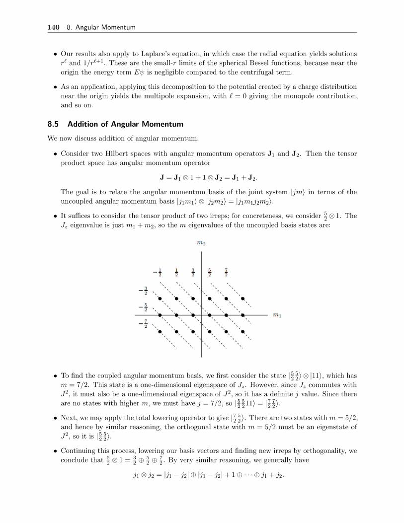
140 8. Angular Momentum
• Our results also apply to Laplace’s equation, in which case the radial equation yields solutions
r` and 1/r`+1. These are the small-r limits of the spherical Bessel functions, because near the
origin the energy term Eψ is negligible compared to the centrifugal term.
• As an application, applying this decomposition to the potential created by a charge distribution
near the origin yields the multipole expansion, with ` = 0 giving the monopole contribution,
and so on.
8.5 Addition of Angular Momentum
We now discuss addition of angular momentum.
• Consider two Hilbert spaces with angular momentum operators J1 and J2. Then the tensor
product space has angular momentum operator
J = J1 ⊗ 1 + 1⊗ J2 = J1 + J2.
The goal is to relate the angular momentum basis of the joint system |jm〉 in terms of the
uncoupled angular momentum basis |j1m1〉 ⊗ |j2m2〉 = |j1m1j2m2〉.
• It suffices to consider the tensor product of two irreps; for concreteness, we consider 52 ⊗ 1. The
Jz eigenvalue is just m1 +m2, so the m eigenvalues of the uncoupled basis states are:
• To find the coupled angular momentum basis, we first consider the state |5252〉 ⊗ |11〉, which has
m = 7/2. This state is a one-dimensional eigenspace of Jz. However, since Jz commutes with
J2, it must also be a one-dimensional eigenspace of J2, so it has a definite j value. Since there
are no states with higher m, we must have j = 7/2, so |525211〉 = |72
72〉.
• Next, we may apply the total lowering operator to give |7252〉. There are two states with m = 5/2,
and hence by similar reasoning, the orthogonal state with m = 5/2 must be an eigenstate of
J2, so it is |5252〉.
• Continuing this process, lowering our basis vectors and finding new irreps by orthogonality, we
conclude that 52 ⊗ 1 = 3
2 ⊕52 ⊕
72 . By very similar reasoning, we generally have
j1 ⊗ j2 = |j1 − j2| ⊕ |j1 − j2|+ 1⊕ · · · ⊕ j1 + j2.
141 8. Angular Momentum
• We define the Clebsch-Gordan coefficients as the overlaps 〈j1j2m1m2|jm〉. These coefficients
satisfy the relations ∑m1m2
〈jm|j1j2m1m2〉〈j1j2m1m2|j′m′〉 = δjj′δmm′ ,
∑jm
〈j1j2m1m2|jm〉〈jm|j1j2m′1m′2〉 = δm1m′1δm2m′2
which simply follow from completeness of the coupled and uncoupled bases. In addition we
have the selection rule
〈jm|j1j2m1m1〉 ∝ δm,m1+m2 .
We may also obtain recurrence relations for the Clebsch-Gordan coefficients by applying J− in
both the coupled and uncoupled bases.
• Next, we consider the operation of rotations. Since J1 and J2 commute,
U(n, θ) = e−iθn·(J1+J2)/~ = U1(n, θ)U2(n, θ)
where the Ui are the individual rotation operators. Then
U |j1j2m1m2〉 =∑jm
∑m′
|jm′〉Djm′m〈jm|j1j2m
′1m′2〉
in the coupled basis, and
U |j1j2m1m2〉 = U1|j1m1〉U2|j2m2〉 =∑m′1m
′2
|j1j2m′1m′2〉Dj1m′1m1
Dj2m′2m2
in the uncoupled basis. Combining these and relabeling indices, we have
Dj1m1m′1
Dj2m2m′2
=∑jmm′
〈j1j2m1m2|jm〉Djmm′〈jm
′|j1j2m′1m′2〉
which allows products of D matrices to be reduced.
Example. Combining spin and spatial degrees of freedom for the electron. We must work in the
tensor product space with basis |r,m〉. Wavefunctions are of the form
ψ(r,m) = 〈r,m|ψ〉
which is often written in the notation
ψ(r) =
ψs(r)
ψs−1(r)...
ψ−s(r)
which has a separate wavefunction for each spin component, or equivalently, a spinor for every
position in space. The inner product is
〈φ|ψ〉 =∑m
∫d3rφ∗(r,m)ψ(r,m).

142 8. Angular Momentum
In the case of the electron, the Hamiltonian is the sum of the spatial and spin Hamiltonians we
have considered before,
H =1
2m(p− qA)2 + qφ− µ ·B, µ=
g
2µσ.
This is called the Pauli Hamiltonian and the resulting evolution equation is the Pauli equation. In
practice, it looks like two separate Schrodinger equations, for the two components of ψ, which are
coupled by the µ ·B term.
The Pauli equation arises from expanding the Dirac equation to order (v/c)2. The Dirac
equation also fixes g = 2. Further terms can be systematically found using the Foldy–Wouthuysen
transformation, as described here. At order (v/c)4, this recovers the fine structure corrections we
will consider below.
Note. The probability current in this case can be defined as we saw earlier,
J = Reψ†vψ, v =1
m(−i~∇− qA) .
Mathematically, J is not unique, as it remains conserved if we add any divergence-free vector field;
in particular, we can add any curl. But the physically interesting question is which possible J
is relevant when we perform a measurement. Performing a measurement of abstract “probability
current” is meaningless, in the sense that there do not exist detectors that couple to it. However,
in the case of a spinless charged particle, we can measure the electric current, and experiments
indicate it is Jc = eJ where J is defined as above; this gives J preference above other options.
However, when the particle has spin, the situation is different. By a classical analogy, we would
expect to regard M = ψ†µψ as a magnetization. But a magnetization gives rise to a bound current
Jb = ∇×M, so we expect to measure the electric current
Jc = eJ +∇× (ψ†µψ).
This is indeed what is seen experimentally. For instance, without the second term, magnetic fields
could not arise from spin alignment, though they certainly do in ferromagnets.
Example. The Landau–Yang theorem states that a massive, spin 1 particle can’t decay into two
photons. This places restrictions on the decay of, e.g. some states of positronium and charmonium,
and the weak gauge bosons. To demonstrate this, work in the rest frame of the decaying particle. By
energy and momentum conservation, after some time, the state of the system will be a superposition
of the particle still being there, and terms involving photons coming out back to back in various
directions and polarizations, |k, e1,−k, e2〉.Now, pick an arbitrary z-axis. We will show that photons can’t come out back to back along this
axis, i.e. that terms |kz, e1,−kz, e2〉 cannot appear in the state. Since z is arbitrary, this shows
that the decay can’t occur at all. The ei can be expanded into circular polarizations,
e1R = e2L = x + iy, e1L = e2R = x− iy
where these two options have Jz eigenvalues ±1. Since |Jz| ≤ 1 for a spin 1 particle, the Jzeigenvalues of the two photons must be opposite, so the allowed polarization combinations are
|kz, e1R,−kz, e2R〉 and |kz, e1L,−kz, e2L〉, giving Jz = 0. Now consider the effect of a rotation
Ry(π/2). Both of these states are eigenstates of this rotation, with an eigenvalue of 1. But the
Jz = 0 state of a spin 1 irrep flips sign, as can be seen by considering the transformation of Y10(θ, φ),
so the term is forbidden. Similar reasoning can be used to restrict various other decays; further
constraints come from parity.
143 8. Angular Momentum
8.6 Tensor Operators
Classically, we say the position x is a vector because of how it transforms under rotations. In
quantum mechanics, observables correspond to operators, motivating us to consider how operators
transform under rotations.
• States transform as |ψ〉 → |ψ′〉 = U(R)|ψ〉. Under a rotation, an operator A becomes
A′ = U(R)AU(R)†
so that 〈ψ′|A′|ψ′〉 = 〈ψ|A|ψ〉.
• A scalar operator K is any operator invariant under rotations, K ′ = K. Therefore K commutes
with all rotations, or, taking the case of an infinitesimal rotation, K commutes with J. One
important example is the Hamiltonian in a central force problem.
• A vector operator V is a triplet of operators satisfying
〈ψ′|V|ψ′〉 = R〈ψ|V|ψ〉.
That is, V corresponds to a classical vector quantity. Expanding in components yields
U(R)ViU(R)† = VjRji.
Taking infinitesimal rotations on both sides gives the commutation relations
[Ji, Vj ] = i~εijkVk
which serves as an alternate definition of a vector operator.
• Similarly, we may show that the dot product of vector operators is a scalar operator, the cross
product is a vector operator, and so on. For example, p2 is a scalar operator and L = r × p
is a vector operator. The adjoint formula shows that angular momentum is always a vector
operator.
• Similarly, we define a rank-2 tensor operator as one that transforms by
U(R)TijU(R)† = TklRkiRlj .
For example, the outer product of vector operators Tij = ViWj is a tensor operator. A physical
example of a rank-2 tensor operator is the quadrupole moment.
Next, we turn to an apparently unrelated subject: the spherical basis of R3.
• Starting with the Cartesian basis x, y, z, we define the spherical basis vectors
e1 = − x + iy√2
, e0 = z, e−1 =x− iy√
2.
We may expand vectors in this basis (or technically, the basis e∗q) by
X = e∗qXq, Xq = eq ·X

144 8. Angular Momentum
• As an example application, consider calculating the dipole transition rate, which is proportional
to 〈n′`′m′|x|n`m〉. This is messy, but a simplification occurs if we expand x in the spherical
basis, because
rY1q(Ω) =
√3
4πxq.
Then the matrix element factors into an angular and radial part,
〈n′`′m′|xq|n`m〉 =
∫ ∞0
r2dr R∗n′`′(r)rRn`(r)×√
4π
3
∫dΩY ∗`′m′(Ω)Y1q(Ω)Y`m(Ω).
This is a substantial improvement: we see that n and n′ only appear in the first factor, while
m and m′ only appear in the second. Furthermore, the integral vanishes automatically unless
m′ = q +m, which significantly reduces the work that must be done. Even better, the angular
part is the same for all rotationally symmetric systems; the radial part factors out what is
specific to hydrogen.
• The ‘coincidence’ arises because both the spherical harmonics and spherical basis arise out of
the representation theory of SU(2). The Ylm’s are the standard angular momentum basis for
the action of rotations on functions on the sphere. Similarly, the spherical basis is the standard
angular momentum basis for the action of rotations in space, which carries the representation
j = 1.
• More generally, tensor quantities carry representations of SO(3) classically, and hence tensor
operators carry representations of SU(2) in quantum mechanics. Hence it is natural for the
photon, which is represented by the vector A classically, to have spin 1.
• Tensor operators can be broken down into irreps. Scalar and vector operators are already irreps,
but the tensor operator Tij = ViWj contains the scalar and vector irreps
trT = V ·W, X = V ×W.
The remaining degrees of freedom form a five-dimensional irrep, the symmetric traceless part
of Tij . This is in accordance with the Clebsch-Gordan decomposition 1⊗ 1 = 0⊕ 1⊕ 2. The
same decomposition holds for arbitrary Tij by linearity.
• Irreps in the standard basis transform by the same D matrices that we introduced earlier. For
example, an irreducible tensor operator of order k is a set of 2k + 1 operators T kq satisfying
UT kq U† = T kq′D
kq′q(U).
An irreducible tensor operator of order k transforms like a spin j particle. In our new language,
writing x in terms of the xq is just writing it as an irreducible tensor operator of order 1.
• Rotations act on kets by multiplication by U(R), while rotation act on operators by conjugation,
which turns into commutation for infinitesimal rotations. Therefore the angular momentum
operators affect the irreducible tensor operator T kq exactly as they affect the kets |kq〉, but with
commutators,
[Jz, Tkq ] = ~kT kq , [Ji, [Ji, T
kq ]] = ~2k(k + 1)T kq .
We don’t even have to prove this independently; it just carries over from our previous work.
145 8. Angular Momentum
• In the case of operators, there’s no simple ‘angular momentum operator’ as in the other cases,
because it would have to be a superoperator, i.e. a linear map of operators.
Note. The ideas above can be used to understand higher spherical harmonics as well. The functions
x, y, and z form an irrep under rotations, and hence the set of homogeneous second-order polynomials
forms a representation as well. Using the decomposition 1⊗ 1 = 0⊕ 1⊕ 2 yields a five-dimensional
irrep, and dividing these functions by r2 yields the ` = 2 spherical harmonics.
This explains the naming of chemical orbitals. The p orbitals are px, py, and pz, corresponding
to angular parts x/r, y/r, and z/r. Note that this is not the standard angular momentum basis;
the functions are instead chosen to be real and somewhat symmetrical. The names of the d orbitals
are similar, though dz2 should actually be called d3z2−r2 .
We now state the Wigner–Eckart theorem, which simplifies matrix elements of irreducible tensor
operators.
• Consider a setup with rotational symmetry, and work in the basis |γjm〉. A scalar operator K
commutes with both Jz and J2, and hence preserves j and m. Moreover, since it commutes
with J±, its matrix elements do not depend on m,
〈γ′j′m′|K|γjm〉 = δj′jδm′mCjγ′γ .
This implies, for instance, that the eigenvalues come in multiplets of degeneracy 2j + 1. We’ve
already seen this reasoning before, for the special case K = H, but the result applies for any
scalar operator in any rotationally symmetric system.
• More generally, the Wigner–Eckart theorem states that
〈γ′j′m′|T kq |γjm〉 = 〈γ′j′||T k||γj〉〈j′m′|jkmq〉
where the first factor is called a reduced matrix element, and the second is a Clebsch-Gordan
coefficient. The reduced matrix element is not a literal matrix element, but just stands in for a
quantity that only depends on T k and the γs and js.
• The Wigner–Eckart theorem factors the matrix element into a part that depends only on the
irreps (and hence depends on the detailed dynamics of the system), and a part that depends
on the m’s that label states inside the irreps (and hence is determined completely by rotational
symmetry). This simplifies the computation of transition rates, as we saw earlier. Fixing the
γ’s and j’s, there are generally (2j + 1)(2j′ + 1)(2k + 1) matrix elements to compute, but we
can just compute one, to get the reduced matrix element.
• The intuition for the Clebsch-Gordan coefficient is that T kq |jm〉 transforms under rotations just
like the ket |kq〉|jm〉. The Clebsch-Gordan factor also provides several selection rules,
m′ = m+ q, j′ ∈ |j − k|, . . . , j + k
just as we saw for dipole transitions with the spherical basis.
• If there is only one irrep, then all irreducible tensor operators of order k must be proportional
to each other. To show this directly, note that all such operators must be built out of linear
combinations of |m〉〈m′|. This set of operators transforms as
j ⊗ j = 0⊕ 1⊕ . . .⊕ 2j.

146 8. Angular Momentum
Hence there is a unique irreducible tensor operator for all spins up to 2j, and none above that.
This shows, for example, that we must have µ∝ S for spins.
• For example, an alpha particle is a nucleus whose ground state has spin zero. Restricting our
Hilbert space to this irrep, the selection rules show that every irreducible tensor operator with
k > 0 must be zero. Thus alpha particles cannot have a magnetic dipole moment.
• To compute the reduced matrix elements of J itself, note that
〈γ′j′m′|Jz|γjm〉 = 〈γ′j′||J ||γj〉〈j′m′|j1m0〉.
The left-hand side is easy to evaluate, giving
〈γ′j′||J ||γj〉 =δγ′γδj′j~m〈jm|j1m0〉
= δγ′γδj′j~√`(`+ 1)
where the last step uses explicit Clebsch-Gordan coefficients for the j ⊗ 1 case.
One useful corollary of the Wigner–Eckart theorem is the projection theorem.
• To prove the theorem directly, one can show the identity
[J2, [J2,V]] = ~2(2(J2V + VJ2)− 4(V · J)J
)for any vector operator V, directly using the definitions.
• We now sandwich this identity between 〈γ′jm′| and |γjm〉. Since the same j value is on both
sides, the left-hand side vanishes, giving
2〈γ′jm′|J2V + VJ2|γjm〉 = 4〈γ′jm′|(V · J)J|γjm〉.
Rearranging slightly, this implies that
〈γ′jm′|V|γjm〉 =1
j(j + 1)~2〈γ′jm′|(V · J)J|γjm〉
which is known as the projection theorem. Intuitively, the right-hand side is the projection of
V “in the J direction”, and the result says that the result is the same as V when we restrict to
a subspace of constant j. This is a generalization of the idea above that, for constant γ and j,
there is only one vector operator.
• The projection theorem can also be applied by explicitly evaluating the reduced matrix element
in the Wigner–Eckart theorem. Since the right-hand side involves the product of a scalar and
vector operator, we first seek to simplify such products.
• Let A be a vector operator and let f be a scalar operator. The Wigner–Eckart theorem says
〈γ′j′m′|Aq|γjm〉 = 〈γ′j′||A||γj〉〈j′m′|j1mq〉
and
〈γ′j′m′|fAq|γjm〉 = 〈γ′j′||fA||γj〉〈j′m′|j1mq〉.
147 8. Angular Momentum
Furthermore, since f is a scalar, we have
〈γ′j′m′|f |γjm〉 = δm′mδj′j〈γ′j||f ||γj〉.
Combining these results gives a decomposition for the reduced matrix elements of fA,
〈γ′j′||fA||γj〉 =∑
Γ
〈γ′j′||f ||Γj′〉〈Γj′||A||γj〉
which makes sense: both A and f can move between irreps, though only A can change j.
• By similar reasoning, for the dot products of vector operators, we have
〈γ′j′||A ·B||γj〉 =∑Γj′
〈γ′j||A||Γj′〉〈Γj′||B||γj〉
where we used A ·B =∑
q AqB†q and the Wigner–Eckart theorem twice.
• Now we can simply show the projection theorem directly. We have
〈γ′j′m′|(A · J)Jq|γjm〉 = δj′j~√j(j + 1)〈jm′|j1mq〉〈γ′j||A · J||γj〉
= δj′j~√j(j + 1)〈jm′|j1mq〉〈γ′j||A||γj〉〈γj||J ||γj〉
= δj′j~2j(j + 1)〈jm′|j1mq〉〈γ′j||A||γj〉= δj′j~2j(j + 1)〈γ′jm′|Aq|γjm〉
where we used the decompositions above and the reduced matrix elements of J.

148 9. Discrete Symmetries
9 Discrete Symmetries
9.1 Parity
In the previous section, we studied proper rotations. We now add in parity, an improper rotation,
and consider its representations.
• In classical mechanics, the parity operator P inverts all spatial components. It has matrix
representation −I, satisfies P 2 = I, and commutes with all proper rotations, PRP−1 = R.
• In quantum mechanics, we look for a parity operator π = U(P ) which satisfies
π†π = 1, π2 = 1, πU(R)π† = U(R).
Mathematically, these conditions mean that we are looking for unitary representations of O(3).
Combining the first postulates show that π is Hermitian, so the parity is observable. The third
postulate is equivalent to [π,J] = 0, i.e. that π is a scalar operator.
• The above postulates rule out projective representations. These are allowed in principle, but
won’t be necessary for any of our applications.
• For a spinless particle, we have previously defined U(R)|x〉 = |Rx〉. Similarly, we may define
π|x〉 = −|x〉, which obeys all of the postulates above. We may also explicitly compute
πxπ† = −x, πpπ† = −p, πLπ† = L
where L is the orbital angular momentum r× p. the parity of the state |lm〉 is (−1)l.
• Another example is a spin-s particle with no spatial wavefunction. The states are |sm〉 for
m = −s, . . . , s. Since π is a scalar operator, we must have
π|sm〉 = η|sm〉
for some constant η = ±1. In nonrelativistic quantum mechanics, the sign has no physical
consequences, so we choose η = 1 so that parity does nothing to the spin state. Adding back
the spatial degrees of freedom gives π|x,m〉 = |−x,m〉.
• In relativistic quantum mechanics, the sign of η makes a physical difference because particle
number can change, but the overall parity must be conserved; this provides some selection rules.
For example, the fact that the photon has negative parity is related to the fact that the parity
of an atom flips during an electric dipole transition, which involves one photon.
• Given a vector operator V, if
πVπ† = ±V
then we say V is a true/polar vector if the sign is −1, and a pseudovector/axial vector if the
sign is +1. For example, x and p are polar vectors but L is an axial vector.
• Similarly, for a scalar operator K, if
πKπ† = ±K
then K is a true scalar if the sign is +1 and a pseudoscalar if the sign is −1. For example, p ·Sis a pseudoscalar.
149 9. Discrete Symmetries
• Note that E is a polar vector while B is an axial vector. In particular, adding an external
magnetic field does not break parity symmetry.
Next, we consider the consequences of parity symmetry of the Hamiltonian.
• Parity is conserved if [π,H] = 0. This is satisfied by the central force Hamiltonian, and more
generally to any system of particles interacting by pairwise forces of the form V (|ri − rj |).
• Parity remains conserved when we account for relativistic effects. For example, such effects
lead to a spin-orbit coupling L · S, but this term is a true scalar. Parity can appear to be
violated when photons are emitted (or generally when a system is placed in an external field),
but remains conserved as long as we account for the parity of the electromagnetic field.
• Parity is also conserved by the strong interaction, but not by the weak interaction. The weak
interaction is extremely weak at atomic energy scales, so parity symmetry is extremely accurate
in atomic physics.
• Just like rotational symmetry, parity symmetry can lower the dimensionality of a system. If
[π,H] = 0, then we can split the Hilbert space into representations with +1 and −1 parity and
diagonalize H within them separately, which is more computationally efficient.
• In the case of rotational symmetry, every rotational irrep has definite parity since π is a scalar
operator. In particular, if there is no degeneracy of irreps, then every energy eigenstate is
automatically a parity eigenstate.
• For example, in hydrogen, the 2s and 2p irreps are degenerate, with even and odd parity. A
linear combination of these states gives an energy eigenstate without definite parity.
• As another example, consider one-dimensional motion in an even potential. Assuming no
degeneracy (which is true for bound states), every eigenstate is either even or odd. However, for
the free particle we have the eigenstates e±ikx which do not have definite parity; the combinations
sin(kx) and cos(kx) do.
Example. Selection rules for electric dipole transitions. Such a transition is determined by the
matrix element 〈n′`′m′|x|n`m〉. It must be parity invariant, but under parity it picks up a factor
of (−1)`+`′+1, giving the selection rule ∆` = odd. The Wigner–Eckart theorem rules out |∆`| > 1,
so we must have ∆` = ±1. The Wigner–Eckart theorem also gives |∆m| ≤ 1.
Example. A spin-orbit coupling. Consider a particle with spatial state |n`m`〉, which separates
into a radial and angular part |n`〉|`m`〉, and a spin state |sms〉. Ignoring the radial part, which
separates out, we consider the total spin states
|`jmj〉 =∑m`,ms
|`m`〉|sms〉〈`sm`ms|jmj〉.
The wavefunction of such a state takes in an angular coordinate and outputs a spinor. A spin-orbit
coupling is of the form σ · x. Since this term is rotationally invariant, it conserves j and mj . From
the standpoint of the spatial part, it’s like an electric dipole transition, so ∆` = ±1. Thus the
interaction can transfer angular momentum between the spin and orbit, one unit at a time.

150 9. Discrete Symmetries
9.2 Time Reversal
Next, we consider time reversal, which is more subtle because it is realized by an antilinear operator.
We begin with the classical case.
• In Newtonian mechanics, if x(t) is a valid trajectory for a particle in a potential (such as an
external electric field), x(−t) is a valid trajectory as well. Since the velocity is flipped, the
momentum is also flipped, p(t)→ −p(−t).
• This reasoning fails in the case of an external magnetic field. However, if we consider the field
to be internally generated by charges in the system, then time reversal takes
ρ→ ρ, J→ −J, E→ E, B→ −B,
where we suppress time coordinates. This gives an extra sign flip that restores the symmetry.
• Note that this is the opposite of the situation with parity. In this case, J is flipped as well, but
E is flipped while B isn’t.
• In the case of quantum mechanics, we have the Schrodinger equation
i~∂ψ
∂t=
(− ~2
2m∇2 + V (x)
)ψ(x, t).
It is tempting to implement time reversal by taking ψ(x, t)→ ψ(x,−t), but this doesn’t work
because only the left-hand changes sign. However, if we take
ψr(x, t) = ψ∗(x,−t)
then we do get a solution, as we can conjugate both sides. Since position information is in the
magnitude of ψ and momentum information is in the phase, this is simply performing the flip
p→ −p we already did in the classical case.
• In the case of an external magnetic field, we have
i~∂ψ
∂t=
1
2m
[−i~∇− q
cA(x)
]2ψ(x, t)
and we again have a problem, as the terms linear in A are imaginary. As in the classical case,
the fix is to reverse the magnetic field, A→ −A.
We now define and investigate the time reversal operator.
• We define the time reversal operator Θ as
|ψr(t)〉 = Θ|ψ(−t)〉.
Setting t = 0, the time reversal operator takes the initial condition |ψ(0)〉 to the initial condition
for the reversed motion |ψr(0)〉.

151 9. Discrete Symmetries
• Since probabilities should be conserved under time reversal, we postulate
Θ†Θ = 1.
By analogy with classical mechanics, we require
ΘxΘ† = x, ΘpΘ† = −p.
Then the orbital angular momentum also flips, ΘLΘ† = −L.
• We postulate that spin angular momentum flips as well. This can be understood classically by
thinking of spin as just internal rotation. Since µ∝ S, the magnetic moment also flips.
• The above postulates cannot be satisfied by any unitary operator, because
Θ[x, p]Θ† = i~ΘΘ† = i~ = [x, p]
but we must get [x,−p]. However, we can construct Θ if we let it be an antilinear operator, i.e.
an operator that complex conjugates everything to its right. We have already seen this in the
conjugated wavefunction above.
• Generally, Wigner’s theorem states that any map that preserves probabilities,
|〈ψ′|φ′〉| = |〈ψ|φ〉|
must be either unitary or antiunitary. Time reversal is the only symmetry that requires the
latter option.
Working with antilinear operators is delicate, because Dirac notation is made for linear operators.
• Let A be antilinear and let L be linear. The usual rule Lc = c∗L becomes
Ac = c∗A
for any scalar c. Note that the product of antilinear operators is linear.
• We defined the action of L on bras by the rule
(〈φ|L)|ψ〉 = (〈φ|)(L|ψ〉).
However, if we naively extend this to antilinear operators, then 〈φ|A would be an antilinear
functional, while bras must be linear functionals. Thus we add a complex conjugation,
(〈φ|A)|ψ〉 = [(〈φ|)(A|ψ〉)]∗ .
It matters which way an antilinear operator acts, and switching it gives a complex conjugate.
• Next, we define the Hermitian conjugate. For linear operators, we let
〈φ|L†|ψ〉 = [〈ψ|L|φ〉]∗ .
To extend this to antilinear operators, we need to find which way A and A† act. The correct
rule is to flip the direction of action,(〈φ|A†
)|ψ〉 = [〈ψ| (A|φ〉)]∗ .
152 9. Discrete Symmetries
One can check that this behaves correctly when |ψ〉 and |φ〉 are multiplied by scalars. The
rule can be remembered by simply ‘flipping everything’ when taking the Hermitian conjugate.
Equivalently, we simply maintain the rule
(A†|ψ〉) = (〈ψ|A)†
as for linear operators.
• An antiunitary operator is an antilinear operator satisfying
A†A = AA† = 1.
Antiunitary operators preserve probabilities, because
〈ψ′|φ′〉 = (〈ψ|A†)(A|φ〉) =[〈ψ|(A†A|φ〉)
]∗= 〈ψ|φ〉∗.
• It is useful to factor an antilinear operator as A = LK where L is linear and K is a standard
antilinear operator. For example, given a basis |n〉 (say, an eigenbasis of the CSCO Q), we may
define KQ|n〉 = |n〉. Then Kx maps the wavefunction ψ(x) into ψ(x)∗.
Next, we apply time reversal symmetry to specific situations.
• In the case of a spinless system, it can be verified that Kx acts on x and p in the appropriate
manner, so this is the time reversal operator; as we’ve seen, it conjugates wavefunctions.
• Now consider a particle of spin s, ignoring spatial degrees of freedom. Since ΘSΘ† = −S, we
have ΘSzΘ† = −Sz, so Θ flips m, Θ|sm〉 = cm|s,−m〉. On the other hand, we have
ΘS+Θ† = Θ(Sx + iSy)Θ† = −Sx + iSy = −S−
whch yields cm1 = −cm, so that cm = η(−1)s−m. We can absorb an arbitrary phase into η.
The common choice is
Θ|sm〉 = i2m|s,−m〉.
• An alternate way to derive this result is to set K = KSz , so that K is conjugation in the
standard angular momentum basis, then choose L to fix up the commutation relations,
Θ = e−iπSy/~K = Ke−iπSy/~
where the exponential commutes with K because its matrix elements are real.
• Restoring the spatial degrees of freedom,
Θ = Kx,Sze−iπSy/~.
One might wonder why Sy appears. Choosing the Sz basis already breaks rotational invariance;
the remaining symmetry between x and y is broken by phase conventions. Defining Θ is one of
the first places where phase conventions have a nontrivial effect.
• In the case of many particles with spin, we may either multiply the individual Θ’s or replace
Sy and Sz above with the total angular momenta. These give the same result because the
Clebsch-Gordan coefficients are real.

153 9. Discrete Symmetries
• Time reversal invariance holds for any Hamiltonian of the form H = p2/2m+V (x). It is broken
by an external magnetic field, but not by internal fields. For example, the spin-orbit coupling
L · S is time-reversal invariant because both the angular momenta flip.
Finally, we apply time reversal to dynamics.
• First, we verify the time-reversed state obeys the Schrodinger equation. Setting ~ = 1,
i∂t|ψr(t)〉 = i∂tΘ|ψ(−t)〉 = Θ [−i∂t|ψ(−t)〉] .
Writing τ = −t, we have
i∂t|ψr(t)〉 = Θ [i∂τ |ψ(τ)〉] = ΘH|ψ(τ)〉 = (ΘHΘ†)|ψr(t)〉.
Hence the time-reversed state satisfies the Schrodinger equation under the time-reversed Hamil-
tonian. The Hamiltonian itself is invariant under time reversal if [Θ, H] = 0.
• If the Hamiltonian is invariant under time reversal and |ψ〉 is a nondegenerate energy eigenstate,
we must have Θ|ψ〉 = eiθ|ψ〉, where the eigenvalue is a phase because Θ preserves norms. Then
the state eiθ/2|ψ〉 has Θ eigenvalue 1.
For the case of spatial degrees of freedom, this implies that the wavefunctions of nondegenerate
states can be chosen real.
• More generally, Θ can link pairs of degenerate energy eigenstates. One can show that we can
always change basis in this subspace so that both have Θ eigenvalue 1.
For example, for the free particle, e±ikx can be combined into sin(kx) and cos(kx). Orbitals in
chemistry, which are real, and chosen from combinations of the Y`,±m.
• In general, we have
Θ2 = Ke−iπSy/~Ke−iπSy/~ = e−i(2π)Sy/~ =
1 bosons
−1 fermions.
This does not depend on phase conventions, as any phase adjustment cancels itself out.
• When there are an odd number of fermions, Θ2 = −1. Then energy levels must be twofold
degenerate, because if they were not, we would have Θ2|ψ〉 = Θeiθ|ψ〉 = |ψ〉, which contradicts
Θ2 = −1. This result is called Kramer’s degeneracy. For example, |l,m〉 pairs with |l,−m〉,except when m = 0, which only occurs for integer spin.
In general, quantum objects such as atoms and nuclei can have multipole moments, which presents
a useful application of parity, time reversal, and the Wigner–Eckart theorem.
• We recall that the multipole expansion of a classical charge distribution starts as
φ(r) =q
r+
d · rr3
+1
6
∑ij
QijTijr5
+ . . . , Tij = 3xixj − r2δij
where the charge, electric dipole moment, and electric quadrupole moment are
q =
∫dr ρ(r), d =
∫dr ρ(r)r, Qij =
∫dr ρ(r)Tij .
154 9. Discrete Symmetries
• There is a similar expansion for the vector potential, but the monopole term vanishes, and we
won’t consider any situations where the quadrupole term matters, leaving the dipole term,
A(r) =µ× r
r3, µ=
1
2
∫dr r× J(r).
• We call the terms in the multipole expansion “2k-poles” for convenience. Formally, the multipole
expansion is just representation theory: a 2k-pole transforms in the spin k irrep, and hence is
described by 2k+1 numbers. Accordingly, at the quantum level, the 2k-poles become irreducible
tensor operators.
• Now restrict to systems described by a single irrep, such as nuclei. In this case, many of the
multipoles are forbidden by symmetry. For example, consider an electric dipole moment d.
Classically, we expect d to flip under P and stay the same under T . But by the Wigner–Eckart
theorem, d ∝ S, which stays the same under P but flips under T . So a permanent electric
dipole moment for a nucleus would violate P and T .
• This argument is actually too quick, because there’s no reason the electric dipole moment of
a quantum system has to behave like our classical intuition suggests. A better argument is to
show that there is no way to extend the definitions of P and T we are familiar with, for classical
objects, to these quantum objects, in such a way that it is a symmetry of the theory.
• To do this, note that our quick argument shows d must transform like S. However, we measure
the effects of d by interaction terms like d ·E, and we know that E must flip under P and stay
the same under T . Hence the term d ·E is odd under both P and T , so the Hamiltonian is not
symmetric.
• Of course, one could just modify how E transforms to get a symmetry of the Hamiltonian, but
that symmetry, even if useful, could not reasonably be called “parity” or “time reversal”. The
E here is a classical electric field whose transformation we should already know.
• Usually people talk about electric dipole moments as violating T , not violating P , even though
they violate both. The reason is that the former is more interesting. By the CPT theorem,
T violation is equivalent to CP violation. While the Standard Model has a lot of known P
violation, it has very little CP violation, so the latter is a more sensitive probe for new physics.
• Note that this argument only applies to particles described by a single irrep. That is, it applies to
neutrons because we are assuming the irreps of nuclei are spaced far apart; there’s no symmetry
that would make the lowest irrep degenerate. But a typical molecule in laboratory conditions
has enough energy to enter many irreps, since the rotational energy levels are closely spaced,
which is why we say, e.g. that water molecules have a permanent electric dipole moment.
• Similar arguments show that electric multipoles of odd k and magnetic multipoles of even k
are forbidden, by both P and T . (However, magnetic monopoles are forbidden for a different
reason.) Hence the leading allowed multipoles are electric monopoles and magnetic dipoles.
• Another rule is that for a spin j irrep, a multipole can only exist if k ≤ 2j. This follows from
the fact that there aren’t irreducible tensor operators for k > 2j on a spin j irrep. For example,
a proton has j = 1/2 and hence cannot have quadrupole moments or higher. We also saw earlier
that an alpha particle has j = 0 and hence cannot have anything but an electric monopole.

155 10. Time Independent Perturbation Theory
10 Time Independent Perturbation Theory
10.1 Formalism
In this section, we cover bound-state perturbation theory.
• Bound-state perturbation theory is a method for finding the discrete part of the spectrum of
a perturbed Hamiltonian, as well as the corresponding eigenstates. It is also known as time-
independent perturbation theory. While the Hamiltonian can have a continuous spectrum as
well, analyzing states in the continuum requires different techniques, such as time-dependent
perturbation theory.
• The most common formulation of bound-state perturbation theory is Rayleigh–Schrodinger
perturbation theory. In this section we will use Brillouin–Wigner perturbation theory, which is
cleaner, but gives the results only implicitly.
• We consider an unperturbed Hamiltonian H0 with eigenvalues εk and eigenstates
H0|kα〉 = εk|kα〉
where α is an index to resolve degeneracies. The Hilbert space splits into eigenspaces Hk.
• We focus on one of the energy levels εn for closer study. Let the full Hamiltonian be H =
H0 + λH1, where λ ∈ [0, 1]. Introducing this parameter gives us a way to continuously turn on
the perturbation, and also a small parameter to expand in.
• Let |ψ〉 be an exact eigenstate with energy E, which “grows out” of the eigenspace Hn as λ
increases,
H|ψ〉 = E|ψ〉.
Both E and |ψ〉 implicitly depend on λ.
• It is useful to define the projectors onto Hn and its orthogonal subspace,
P =∑α
|nα〉〈nα|, Q = 1− P.
Both of these commute with H0.
• If the perturbation is small, then we expect |ψ〉 mostly lies in Hn. Computing P |ψ〉 is “easy”,
while computing the part Q|ψ〉 in all the other Hk is “hard”.
• We will write an expression for Q|ψ〉 using a power series. First, note that
(E −H0)|ψ〉 = λH1|ψ〉.
We could get a formal solution for |ψ〉 by multiplying by (E −H0)−1, which satisfies
1
E −H0=∑kα
|kα〉〈kα|E − εk
.
However, the denominator blows up for k = n as the perturbation is removed.
156 10. Time Independent Perturbation Theory
• Instead, we define a restricted version
R =∑k 6=n,α
|kα〉〈kα|E − εk
.
The denominator could also blow up if E coincides with some εk for k 6= n. We will consider
this case in more detail later.
• The operator R is restricted to the orthogonal complement of Hn, so it is annihilated by P and
unaffected by Q, and
R(E −H0) = (E −H0)R = Q.
• Now, if we instead multiply both sides by R, we find
Q|ψ〉 = λRH1|ψ〉.
Now if we add P |ψ〉 to both sides, we have
|ψ〉 = P |ψ〉+ λRH1|ψ〉.
This equation can be iterated, by plugging it into itself, to give a series,
|ψ〉 =∑s≥0
λs(RH1)sP |ψ〉.
As an example, we consider nondegenerate perturbation theory.
• In this case, there is only a single state |n〉 in Hn. We normalize |ψ〉 so that P |ψ〉 = |n〉, which
implies 〈n|ψ〉 = 1. The series reduces to
|ψ〉 =∑s≥0
λs(RH1)s|n〉.
• Plugging in the definitions, to second order we have
|ψ〉 = |n〉+ λ∑k 6=n,α
|kα〉〈kα|H1|n〉E − εk
+ λ2∑k 6=n,α
∑k′ 6=n,α′
|kα〉〈kα|H1|k′α′〉〈k′α′|H1|n〉(E − εk)(E − εk′)
+ . . . .
We see the expected suppression by energy differences of the contribution of other states.
• To get the energy E, we note that
0 = 〈n|E −H0 − λH1|ψ〉 = E − εn − λ〈n|H1|ψ〉.
The last term can be computed using the series above, giving
E = εn + λ〈n|H1|n〉+ λ2〈n|H1RH1|n〉+ λ3〈n|H1RH1RH1|n〉+ . . .
which can be written explicitly as
E = εn + λ〈n|H1|n〉+ λ2∑k 6=n,α
〈n|H1|kα〉〈kα|H1|n〉E − εk
+ λ3∑k 6=n,α
∑k′ 6=n,α′
〈n|H1|kα〉〈kα|H1|k′α′〉〈k′α′|H1|n〉(E − εk)(E − εk′)
+ . . . .

157 10. Time Independent Perturbation Theory
• This is still an implicit expression, because E appears on both sides. However, we can use it to
extract an explicit series for E. For example, at first order we have
E = εn + λ〈n|H1|n〉+O(λ2).
To go to second order, it suffices to take the first three terms in the series for E, plugging in
the zeroth-order expression for E into the O(λ2) term, giving
E = εn + λ〈n|H1|n〉+ λ2∑k 6=n,α
〈n|H1|kα〉〈kα|H1|n〉εn − εk
+O(λ3)
which is what appears in most textbooks. However, at higher orders the explicit Rayleigh–
Schrodinger expansion begins to look more complicated.
• We can then plug this back into the expansion for |ψ〉. For example, at first order,
|ψ〉 = |n〉+ λ∑k 6=n,α
|kα〉〈kα|H1|n〉εn − εk
+O(λ2)
which is again a standard textbook result.
Now we consider the degenerate case.
• In this case, we must expand P |ψ〉 as
P |ψ〉 =∑α
|nα〉cα
where the coefficients cα are unknown.
• The equation we used above for the energy becomes
0 = 〈nα|E −H0 − λH1|ψ〉 = (E − εn)cα − λ〈nα|H1|ψ〉.
Plugging in the series solution for |ψ〉 gives
(E − εn)cα =∑β
λ〈nα|H1|nβ〉+ λ2∑k 6=n,γ
〈nα|H1|kγ〉〈kγ|H1|nβ〉E − εk
+ . . .
cβ.
Regarding the quantity in brackets as a g × g matrix, where g = dimHn is the degeneracy, we
see that the energies E are determined by the eigenvalues of this matrix, and the states (each
specified by a set of coefficients cα) corresponds to the eigenvectors. The extra complication is
that E also appears in the matrix elements.
• Often, we will only want the first order effect. In this case, the eigenvectors are just those of
H1 restricted to Hn, and the energy shifts are just the corresponding eigenvalues of H1.
• Sometimes, some or all of the states will remain degenerate. This degeneracy might be broken
at some higher order. If it’s never broken at any order, than in almost every case we can identify
a symmetry of the full Hamiltonian which is responsible for this.
158 10. Time Independent Perturbation Theory
• To work at second order, we can substitute E with εn in the denominator of the quadratic term,
giving a standard eigenvalue equation. Alternatively, we can treat λ〈nα|H1|nβ〉 as part of the
unperturbed Hamiltonian, as we have presumably already diagonalized it to get the first order
result, and treat the quadratic term as the perturbation in a new, lower-dimensional problem.
• Once we have E and the cα to some order, we know P |ψ〉, and we can simply plug this into
our series for |ψ〉 to get the full state to the same order.
• Sometimes, one is concerned with “nearly degenerate” perturbation theory, where some energy
levels are very close in the unperturbed Hamiltonian. Then even a weak perturbation can cause
the perturbed energy E to cross another unperturbed energy level, causing R to diverge.
• To fix this, we can transfer a small term from H0 and H1 so that these problematic unperturbed
energy levels are exactly degenerate, then use ordinary degenerate perturbation theory. (This
is, of course, what we are implicitly doing whenever we use degenerate perturbation theory at
all, since practically there are always further effects that break the degeneracies.)
• A completely equivalent solution is to define R excluding both Hn and all nearly degenerate
eigenspaces; the resulting series is the same.
Note. Why does a state within a continuum have to be treated with time-dependent perturbation
theory? The point is that the state generally gets “lost” into the continuum, i.e. the true energy
eigenstates have zero overlap with the original unperturbed state. For example, if we prepare an
atom in an excited state but allow it to radiate into vacuum (thus introducing a continuum of states
of the electromagnetic field), then no matter how we prepare the atom, the long-term probability
of occupancy of the state is zero.
10.2 The Stark Effect
As a first example, we consider the Stark effect for both hydrogen and the valence electron in alkali
atoms, using the approximation described previously. We ignore all other effects that could cause
energy level splitting, which we will consider in detail later.
• In hydrogen, the potential is V0(r) = −e2/r and the energy levels are
En = − 1
2n2
e2
a0
while for alkali atoms, the energy levels are En,` with energy increasing with `.
• We take the electric field to be F = F z (to avoid confusion with energy), so the perturbation is
V1 = qΦ = eFz
where the electron charge is q = −e.
• It’s reasonable to treat this as a small perturbation near the nucleus, since electric fields made
in the laboratory are typically much weaker than those in atoms. However, V1 grows for large
r while V0 falls, so the perturbation analysis doesn’t work for states with sufficiently large n.
159 10. Time Independent Perturbation Theory
• Technically, there don’t exist any bound states at all, no matter how small the field F is, because
the potential will become very negative for z → −∞. Hence all states can tunnel over a barrier
and escape to infinity. We’ll ignore this, since for small n, the barrier width grows as 1/F ,
and hence the tunneling rate falls very quickly as F is decreased. More precisely, it can be
calculated using the WKB approximation.
Now we consider some basic examples.
• The ground state of hydrogen is |100〉, while the ground state of an alkali atom is |n00〉. There
is no linear (i.e. first order) Stark effect in this case, because
∆E(1)g = 〈n00|eFz|n00〉 = 0
by parity, since the states have definite parity and z is odd under parity. We saw a similar
conclusion when discussing electric dipole transitions above.
• The linear Stark effect can only occur if the corresponding eigenstate has a permanent dipole
moment d. Classically, we expect that ∆E = −d · F. Quantum mechanically, the dipole
moment operator and linear energy shift are
d = qx = −ex, ∆E(1) = −〈d〉 · F.
However, 〈d〉 must vanish for any nondegenerate energy eigenstate, simply because parity leaves
the energy invariant but flips d. Hence to see a linear Stark effect, we require degenerate states.
• In a generic alkali atom, only states of the same n and ` are degenerate. But as we argued
earlier, the operator z has to change ` by ±1, so again there is no linear Stark effect. More
generally, we need systems with degenerate SU(2) multiplets with opposite parities.
• Now consider the excited states of hydrogen. We focus on the states with principal quantum
number n, which are n2-fold degenerate. The linear Stark effect depends on the matrix elements
〈n`m|eFz|n`′m′〉.
As shown earlier, we must have ∆` = ±1, and since z is invariant under rotations about the z-
axis, m = m′. For example, for n = 2, the only states that can be connected by the perturbation
are |200〉 and |210〉.
• By using the explicit hydrogen wavefunctions, we have
〈200|eFz|210〉 = −W, W = 3eFa0.
The energy W is of the order of the energy needed to shift the electron from one side of the
atom to the other. This is because |210〉 has two symmetric lobes, of positive and negative z.
Adding on |200〉 will make one lobe grow and the other shrink, depending on the phase.
• Restricting to these two states, the perturbation matrix is(0 −W−W 0
)
160 10. Time Independent Perturbation Theory
so the first-order energy shifts are ∆E(1)2 = ±W . The n = 2 energy level splits into three, with
the new eigenstates
|±W 〉 =1√2
(|200〉 ∓ |210〉)
and the states |211〉 and |21,−1〉 remaining degenerate at this order.
• This degeneracy remains at all orders, and can be explained using symmetries. In fact, it turns
out that this degeneracy can be explained by the surviving subset of the SO(4) symmetry of
the hydrogen atom. However, the degeneracy can also be explained more simply by noting that
Lz and time reversal Θ commute with H.
• From Lz, we know the energy eigenstates can be labeled as |γm〉 where γ is an additional index.
We also know that Θ flips the sign of m. Hence all states with m 6= 0 are at least doubly
degenerate.
• This result should not be confused with Kramer’s degeneracy, which applies to systems without
rotational symmetry but an odd number of fermions. Since we have neglected the electron’s
spin, its fermionic nature never came into play above.
Example. In the H+2 molecule, the protons can be treated as roughly fixed. Then there is rotational
symmetry along the axis connecting them, causing two-fold degeneracy for m 6= 0 states as above.
However, in reality the protons are free to move, causing a small splitting known as “Λ-doubling”,
where Λ is the standard name for the magnetic quantum number of the electrons about the axis of
a diatomic molecule.
We now continue discussing the Stark effect in hydrogen.
• In the absence of an external field, the 2p level of hydrogen decays quickly to 1s, with a lifetime
on the order of 10−9 seconds. But the 2s state has a much longer lifetime of 10−1 seconds,
because it decays to 1s by emitting two photons. This makes it easy to prepare a population
of 2s and 1s states.
• However, by turning on an electric field, the 2s and 2p states rapidly evolve into each other.
When such a field is applied to a population of 2s hydrogen atoms, the result is a rapid burst
of photons.
• Now we return to the ground state and consider the first order wavefunction shift. The result is
|ψ〉 = |100〉+∑
n`m 6=100
|n`m〉〈n`m|eFz|100〉E1 − En
.
This state has an induced dipole moment.
• If we define the polarizability α by the first-order response to the field,
〈d〉 = αF +O(F 2)
then we have
α = −2e2∑
n`m 6=100
〈100|z|n`m〉〈n`m|z|100〉E1 − En
.
More generally, the polarizability could be a tensor, 〈di〉 = αijFj +O(F 2). We can convert the
polarizability of an atom to a dielectric constant of a gas using the Clausius-Mossotti formula.
161 10. Time Independent Perturbation Theory
• Next, we can compute the energy shift of the ground state to second order, i.e. the quadratic
Stark effect. The result is
∆E(2)g =
∑n`m 6=100
〈100|eFz|n`m〉〈n`m|eFz|100〉E1 − En
= −1
2αF 2 = −1
2〈d〉 · F.
This factor of 1/2 is exactly as expected, because the dipole moment is induced, rather than
permanent; it grows linearly with F as F is turned on.
• Calculating α is a little tricky, because we must sum over an infinite number of intermediate
states, including the ionized continuum states. However, a crude estimate can be done using
En − E1 > E2 − E1 =3
8
e2
a0
which implies
α <2e2
E2 − E1
∑n`m
〈100|z|n`m〉〈n`m|z|100〉
where we have removed the restriction on the sum since the additional term doesn’t contribute
anyway. Recognizing a resolution of the identity,
α <2e2
E2 − E1〈100|z2|100〉 =
2e2
E2 − E1a2
0 =16
3a3
0.
In fact, the exact answer is α = (9/2)a30. We could have guessed that α ∼ a3
0 from a classical
model, e.g. thinking of the electron as a mass on a spring, but only this calculation gives us
the coefficient.
• Above, we have discussed a stark difference between a system with degeneracy and a system
without: a lack of degeneracy guarantees no linear Stark effect. But in real life, degeneracy
is never perfect. More precisely, if the degeneracy is weakly broken by some other physics,
then the Stark effect will be quadratic in the regime where that other physics dominates, and
linear when the Stark effect dominates. This is just the case for hydrogen, where the 2s and 2p
degeneracy is already broken by the Lamb shift.
• A more formal way to say this is that the full Hamiltonian can be written as H0 plus a
possibly large number of small perturbations. To get the right answer, we should account for
the most important perturbation first, then treat the next-most important perturbation as a
perturbation on the result, and so on. Of course the physical answer doesn’t depend on how
we do the ordering, but if we choose it wrong, then our resulting series won’t be good.
• In chemistry, one often speaks of molecules with permanent electric dipole moments. This
doesn’t violate parity; it simply means that two energy levels of opposite parity are close
enough that even a small electric field takes the Stark effect into the linear regime; however,
as long as the energy levels are not exactly degenerate (which will always be the case) there is
also a quadratic regime at low fields.
162 10. Time Independent Perturbation Theory
10.3 Fine Structure
Next we consider fine structure, which concerns the effects of relativity and spin. These appear at
the same order, namely (v/c)2, so they must be treated together. They may also be derived in a
unified way from the Dirac equation, though we do not do this here.
• There are three new terms: the relativistic kinetic energy correction, the Darwin term, and the
spin-order term,
HFS = HRKE +HD +HSO.
• The first correction comes from the relativistic kinetic energy,
E =√m2c4 + p2c2 = mc2 +
p2
2m− p4
8m3c2+ . . . .
• The spin-orbit coupling term is
HSO = −1
2µ ·B′
where B′ is the magnetic field as seen in the electron’s momentary rest frame. The factor of
1/2 is because the electron’s frame is not inertial, and half of the effect is cancelled out by
Thomas precession. This is a tricky calculation; in any case the result can also be extracted
straightforwardly from the Dirac equation.
• In the lab frame, we have
E =1
e∇V =
1
e
1
r
dV
drx, B = 0.
The leading order field transformations when the electric field dominates are
E′ = E, B′ = −v
c×E.
• Since we are interested in the leading effect, we plug in p = mv to find
B′ =1
emc
1
r
dV
drL
where L = x×p is the orbital angular momentum of the electron. Finally, using µ= −(e/mc)S
with the leading order result g = 2, we have
HSO =1
2m2c2
1
r
dV
drL · S.
• Finally, the Darwin term arises because the electron’s location is smeared on the order of
the Compton wavelength λ = ~/mc. This means the electron really feels the average of the
electrostatic potential over a region of radius λ. By the harmonic property of the Laplacian,
this gives a correction proportional to λ2∇2V .
• A genuine derivation using the Dirac equation gives the coefficient,
HD =1
8
~2
m2c2∇2V.
At the level of the Dirac equation, the Darwin term comes from interference between positive
and negative frequency components. These cause rapid oscillations at the Compton frequency,
known as Zitterbewegung, that smooth out the location of the electron.
163 10. Time Independent Perturbation Theory
• We now specialize to atomic units ~ = m = e = 1, where α = 1/c ≈ 1/137. In this case,
HRKE = −α2
8p4, HD =
α2
8∇2V, HSO =
α2
2
1
r
dV
drL · S
and it is clear the terms are all of the same order.
• We can specialize further to one-electron atoms, where
V (r) = −Zr,
1
r
dV
dr=Z
r3, ∇2V = 4πZδ(x)
and the last two terms become
HD = Zα2π
2δ(x), HSO =
Zα2
2
1
r3L · S.
Note that a factor of Z has appeared in HD because Zδ(x) is the charge density of the nucleus.
• As we will see below, the energy shifts will all be proportional to (Zα)2. In fact, the full
expansion from the Dirac equation is a series in (Zα)2, and hence is good when Zα 1. For
heavy atoms such as uranium, it is better to use a fully relativistic treatment.
Next, we discuss the choice of basis.
• Since we are now dealing with spin, we include the spin magnetic quantum number, giving the
unperturbed basis |n`m`ms〉 which simultaneously diagonalizes L, L2, S, and S2. The energy
levels are En = −Z2/2n2.
• In general, it is useful to choose a basis which diagonalizes observables that commute with the
full Hamiltonian. If we choose the basis naively, we will have to diagonalize a 2n2× 2n2 matrix,
while if we choose it well, we get selection rules which break the matrix into smaller pieces.
• As such, it may be useful to consider the total angular momentum J = L + S. Since HRKE is a
scalar, it commutes with L. Since it only depends on the orbital motion, it commutes with S,
and hence with J. Similarly, HD commutes with all of these operators. But we have
[L, HSO] 6= 0, [S, HSO] 6= 0
but [J, HSO] = 0, since J rotates the entire system. Furthermore, HSO commutes with L2 and
S2 because, for example, [L2,L · S] = [L2,L] · S = 0.
• Hence we are motivated to work in the “coupled basis” |n`jmj〉 which simultaneously diagonal-
izes L2, S2, J2, and Jz. This is related to the original basis by Clebsch-Gordan coefficients,
|n`jmj〉 =∑m`,ms
|n`m`ms〉〈`sm`ms|jmj〉
and we will suppress s below. Since all three fine structure terms are diagonal in the coupled
basis, there is no need to do degenerate perturbation theory; we just have to compute their
diagonal matrix elements. (There is no point in going to second order perturbation theory,
since there are other effects that are more important at first order.)
164 10. Time Independent Perturbation Theory
Now we proceed to computing the energy shifts.
• It’s easier to think about HRKE in the uncoupled basis, then transform to the coupled basis.
This term is purely orbital and commutes with L2, so
〈n`m`ms|HRKE|n`′m′`m′s〉 = δ``′δmsm′s〈n`m`|HRKE|n`m′`〉.
Since HRKE is a scalar operator, by the Wigner–Eckart theorem we have
〈n`m`|HRKE|n`m′`〉 = δm`m′`〈n`0|HRKE|n`0〉.
• Now, applying Clebsch-Gordan coefficients, and the above results,
〈n`jmj |HRKE|n`jmj〉 =∑m`,ms
∑m′`,m
′s
〈jmj |`m`ms〉〈n`m`ms|HRKE|n`m′`m′s〉〈`m′`m′s|jmj〉
= 〈n`0|HRKE|n`0〉∑m`,ms
〈jmj |`m`ms〉〈`m`ms|jmj〉
= 〈n`0|HRKE|n`0〉
so the coefficients have dropped out completely.
• It remains to calculate the expectation value. This is easiest if we note that
HRKE = −α2
2T 2 = −α
2
2(H0 − V )2
since we know how to calculate the expectation values of H0 and V ,
〈H0〉 = En, 〈V 〉 = −Z⟨
1
r
⟩= −Z
2
n2
where the latter result follows from the virial theorem.
• The difficult part is calculating 〈V 2〉, which requires special function techniques, giving⟨1
r2
⟩=
Z2
n3(`+ 1/2)
which gives a total energy shift of
〈n`jmj |HRKE|n`jmj〉 = (Zα)2(−En)1
n2
(3
4− n
`+ 1/2
).
• By the same reasoning, the Darwin term reduces to
〈n`jmj |HD|n`jmj〉 = 〈n`0|HD|n`0〉 = Zα2 π
2|ψn`0(0)|2.
The shift is only nonzero for ` = 0, where we get a factor of Y00 = 1/√
4π. Using the result
Rn0(0) = 2(Z/n)3/2, we have
〈n`jmj |HD|n`jmj〉 = (Zα)2(−En)1
nδ`0.

165 10. Time Independent Perturbation Theory
• The spin-orbit term is best handled by writing
L · S =1
2(J2 − L2 − S2).
As promised above, this is easy to evaluate in the coupled basis,
〈n`jmj |HSO|n`jmj〉 =Zα2
4(j(j + 1)− `(`+ 1)− s(s+ 1))〈n`jmj |
1
r3|n`jmj〉
where j = `± 1/2.
• By the same reasoning as above, the final factor can be written as
〈n`jmj |1
r3|n`jmj〉 = 〈n`0| 1
r3|n`0〉
and special function techniques give⟨1
r3
⟩=
Z3
n3`(`+ 1/2)(`+ 1).
• In the case ` = 0, the prefactor is zero, but 〈1/r3〉 diverges, so the result is indeterminate. The
proper way to handle this is to regulate the Coulomb singularity, which causes 〈1/r3〉 not to
diverge, giving a result of zero.
• The spin-orbit and Darwin terms both have special cases for ` = 0, contributing or not con-
tributing respectively, but combine into something simple. The total result is
∆EFS = (Zα)2(−En)1
n2
(3
4− n
j + 1/2
).
Remarkably, the answer only depends directly on n and j, so the energy levels are
Enj = − Z2
2n2
(1− (Zα)2
n2
(3
4− n
j + 1/2
)).
The energy levels are shifted downward, and the total energy increases with j. Some degeneracy
remains, indicating a residual symmetry of the system.
We now make some comments about this result.
• As shown here, the Dirac equation gives an exact result for the hydrogen energy levels,
Enj =mc21 +
(Zα
n− j − 1/2 +√
(j + 1/2)2 − (Zα)2
)21/2
which recovers mc2, the ordinary energy levels, and the fine structure when expanded. However,
at the next order additional effects appear which are not captured by the Dirac equation, such
as hyperfine structure and the Lamb shift.

166 10. Time Independent Perturbation Theory
• Some energy levels are shown below, with the fine structure exaggerated for clarity. This
diagram uses spectroscopic notation n`j , where ` = s, p, d, f, . . ..
• The arrows above also show the allowed electric dipole transitions. These are determined by
the matrix elements 〈n`jmj |x|n′`′j′m′j〉. Note that the operator x is a tensor operator of spin
1 with respect to both purely spatial rotations, generated by L, and rotations of the whole
system, generated by J. Applying the Wigner–Eckart theorem gives the constraints
|∆`| ≤ 1, |∆j| ≤ 1, |∆mj | ≤ 1.
Parity gives the additional constraint ∆` 6= 0, since the parity of the coupled states is (−1)`,
but it places no constraint on ∆j.
• The Lamb shift is due to the interaction of the electron with the quantized electromagnetic
field. Its most historically important effect is splitting the degeneracy between 2s1/2 and 2p1/2,
so that 2s1/2 is about 1 GHz higher than 2p1/2. For comparison, fine structure places 2p3/2
about 10 GHz higher. Parametrically, the Lamb shift scales as Enα3 log(1/α).
• Since 2s1/2 cannot participate in electric dipole transitions, the Lamb shift means that its
dominant decay mode is to 2p1/2, upon which the atom quickly decays to 1s1/2.
• In alkali atoms, much of the above reasoning also goes through, except that here the degeneracy
in ` is already strongly split by the non-Coulomb nature of the potential. In this case, the most
important effect is the spin-orbit coupling, because this is the only term that breaks degeneracy
in j. By a similar analysis,
∆ESO =α2
4(j(j + 1)− `(`+ 1)− 3/4)
⟨1
r
dV
dr
⟩.
For example, this term splits the 3p level of sodium to 3p1/2 and 3p3/2. When these levels decay
to 3s, one observes the sodium doublet.
167 10. Time Independent Perturbation Theory
Note. The Lamb shift is just an additional smearing like the Darwin term, which is due to interaction
with vacuum fluctuations. Consider an atom in a large cubical box of side length L. The modes of
the quantum electromagnetic field perpetually have vacuum energy ~ωk, where ωk is their frequency.
These quantum fluctuations form a randomly varying classical electric field Ek, where
|Ek|2L3 ∼ ~ωk
since both sides measure the total field energy in that mode. The random fluctuations change over
a characteristic time τ ∼ 1/ωk, over which the displacement of the particle is
δr ∼ e|Ek|τ2 ∼ e|Ek|ω2k
.
Since the fluctuations of these modes are independent, the mean square fluctuation is
〈δr2〉 ∼∑k
e2|Ek|2
ω4k
∼ e2~∑k
1
(Lωk)3∼ e2~
∫dk
(L
~
)3 1
(Lωk)3∼ e2
~2c3
∫dk
k3
where we used the fact that states are spaced in momentum space by ∆k ∼ ~/L. This integral is
logarithmically divergent, but we should put in cutoffs. Modes with wavelengths larger than the
atom don’t affect the electron much, just pushing on it adiabatically, while modes with wavelengths
smaller than the electron’s Compton wavelength will instead cause new particles to spontaneously
pop out of the vacuum. The ratio between these two scales is α, so
〈δr2〉 ∼ e2
~2c3log
1
α.
Following the same reasoning for the Darwin term, this gives an energy shift of
∆E
En∼ α3 log
1
α
for ` = 0 states. One can use a similar story to justify the Darwin term within quantum field
theory. Instead of interacting with virtual photons, an electron-positron pair suddenly, spontaneously
appears out of the vacuum. The positron annihilates the old electron and the new electron continues
on in its place, effectively allowing the electron’s position to teleport.
One might wonder how much of these amazing stories are actually true. Unfortunately, while
this kind of reasoning is common in popular science, it bears little resemblance to how quantum field
theory actually works. “Quantum fluctuations” do not behave like classical stochastic ones, and the
theory would not make any sense if they did. We only arrive at the correct answer by accident: while
the words above are wrong, the equations happen to have similar dimensions to the real, correct
ones. While this derivation worked, almost all heuristic arguments using quantum fluctuations give
wrong answers. If one took the above statements seriously, as many legitimately curious laypeople
do, one would also conclude, for example, that electrons with definite momentum actually are
randomly battered around by field fluctuations, and hence infinite energy can be extracted from
the vacuum by harnessing the kinetic energy the electrons pick up.
Using fragile and misleading analogies like this is perhaps responsible for the majority of pop-
ular misconceptions about quantum mechanics. Luckily, for practitioners who do know quantum
mechanics, the properties of these supposed fluctuations are so vague that one can just tweak a
“derivation” using them to get any desired answer. This makes them good at providing an “intuitive”
explanation of a real calculation one has already done, but not a good tool when one doesn’t know
the answer in advance.
168 10. Time Independent Perturbation Theory
Note. A quick and dirty derivation of Thomas precession. Consider an electron moving at speed
v c, which is following a straight track, which suddenly turns by an angle θ 1. In the electron’s
frame, the track is length contracted in the longitudinal direction, so it has a larger turn angle,
θ′ = tan−1(γ tan θ) ≈ γθ.
That is, the electron thinks it turns by a larger amount than it does in the lab frame, by
θ′ − θθ≈ γ − 1 ≈ v2
2c2.
If the electron moves uniformly in the lab frame, then the “extra” precession is
ωT =ωv2
2c2=
av
2c2
and thinking a bit about the directions gives
ωT =v × a
2c2.
This is the result for Thomas precession in the nonrelativistic limit. Plugging in a = r(dV/dr)
shows that half of the naive spin-orbit contribution is cancelled, as claimed above. The exact result,
which properly should be derived by integrating infinitesimal Lorentz transformations, is
ωT =γ2
γ + 1
v × a
2c2.
10.4 The Zeeman Effect
Next, we consider the Zeeman effect, involving atoms in magnetic fields.
• We continue to use atomic units, where c = 1/α ≈ 137. This means the Bohr magneton is
µB =e~
2mc=
1
2c=α
2.
Taking the electron g factor to be 2, we hence have
µ= gµBS
~= −αS
so the energy of interaction of an electron spin in a magnetic field is
−µ ·B = αB · S.
• Typical magnetic fields in an atom are, by dimensional analysis in Gaussian units,
B0 =e
a20
=m2e5
~4= 1.72× 10³ T
This is equal to the electric field at the Bohr radius, which in Gaussian units has the same units
as the magnetic field.
169 10. Time Independent Perturbation Theory
• However, the most important quantity for perturbation theory is the magnitude of the force;
magnetic forces are suppressed by a factor of v/c = α relative to electric ones. Hence a magnetic
field perturbation to be comparable in effect to the electrostatic field, we need field strength
B0/α = 2.35 × 10⁵ T, which is much higher than anything that can be made in the lab. As
such, we will always treat the magnetic fields as weak.
• Accounting for fine structure, the Hamiltonian is
H =1
2(p + αA)2 + V (r) +HFS + αB · S.
This differs from our earlier expression because we are using Gaussian and atomic units, where
q = −1. In Gaussian units, since magnetic fields have the same units as electric ones, one can
get them from the SI result by “dividing by c”, accounting for the factor of α in the orbital
piece. This also makes it clear that the spin and orbital pieces both contribute at O(α).
• We take the magnetic field and vector potential to be
B = Bz, A =1
2B× r.
Since this vector potential is in Coulomb gauge, p ·A = A · p, so
T =1
2(p + αA)2 =
p2
2+ αp ·A +
α2
2A2 = T1 + T2 + T3.
• We can simplify T2 by noting that
T2 =α
2p · (B× r) =
α
2B · L, L = r× p
where we used the scalar triple product rule, and there are no ordering issues since ∇ ·B = 0.
• The term T3 can be expanded as
T3 =α2
8B2(x2 + y2)
and hence behaves like a potential. However, it is suppressed by another power of α, and hence
can be dropped.
• The last term is the spin term αB · S. Combining this with T2 gives the total perturbation
HZ =α
2B · (L + 2S) =
α
2B(Lz + 2Sz).
The reason we can’t drop the fine structure contributions is that they scale as α2, while the
Zeeman perturbation scales as αB. As a crude estimate, the two are equally important for field
strengths αB0 ∼ 10 T, which is quite high, though the threshold is actually about a factor of
10 smaller due to suppression by dimensionless quantum numbers.
• On the scale of materials, the spin and T2 terms are responsible for Pauli paramagnetism, while
the T3 term is responsible for Landau diamagnetism; we’ve seen both when covering statistical
mechanics. The Zeeman effect is also used to measure magnetic fields via spectral lines.

170 10. Time Independent Perturbation Theory
First, we consider the strong field case, where HZ dominates. This strong-field Zeeman effect is also
called the Paschen–Back effect. Note that we can’t take the field strength to be too high, or else
the term T3 will become important.
• The first task is to choose a good basis. Since the magnetic field is in the z direction, HZ
commutes with Lz, Sz, and Jz. Furthermore, it commutes with L2 and S2. However, we have
[J2, HZ] 6= 0
because J2 contains L ·S, which in turn contains LxSx+LySy. Thus, the Zeeman effect prefers
the uncoupled basis.
• In the uncoupled basis, the perturbation is already diagonal, so we just read off
∆E =α
2B〈n`m`ms|Lz + 2Sz|n`m`ms〉 =
α
2B(m` + 2ms) = µBB(m` + 2ms).
Note that if one didn’t know about spin, one would expect that a spectral line always splits into
an odd number of lines, since ∆E = µBBm`. Violations of this rule were called the anomalous
Zeeman effect, and were one of the original pieces of evidence for spin. (In fact, a classical model
of the atom can account for three lines, one of the most common cases. The lines correspond
to the electron oscillating along the field, and rotating clockwise and anticlockwise about it.)
• As an example, the n = 2 states of hydrogen behave as shown.
The 2p states |m`ms〉 = |−1, 12〉 and |1,−1
2〉 are degenerate. This degeneracy is broken by QED
corrections to the electron g factor, though this is suppressed by another factor of α. This
result holds identically for alkali atoms.
• For one-electron atoms, some of the 2s states are also degenerate with the 2p states, as |`m`ms〉 =
|0012〉 is degenerate with |101
2〉, and |00,−12〉 with |10,−1
2〉. In total, the eight n = 2 states are
split into five energy levels, three of which have two-fold degeneracy.
• We now consider the impact of fine structure, treating HZ as part of the unperturbed Hamilto-
nian. For simplicity, we only consider the spin-orbit contribution,
HSO = f(r)L · S, f(r) =α2
2
1
r
dV
dr.
This is the conceptually trickiest one, since it prefers the coupled basis, while we must work in
the uncoupled basis |n`m`ms〉, where there are two-fold degeneracies.
171 10. Time Independent Perturbation Theory
• Using this basis is tricky because HSO can modify m` and ms values (though not ` values, since
[L2, HSO] = 0). However, it can only modify m` and ms by at most one unit at a time, since
L · S =1
2(L+S− + L−S+) + LzSz
or by applying the Wigner–Eckart theorem. The 2p degenerate states differ in ms by multiples
of 2, so HSO can’t mix the degenerate states. Hence to calculate the first order shift, it suffices
to look at its diagonal matrix elements.
• Thus, the energy shifts are
∆E = 〈n`m`ms|f(r)L · S|n`m`ms〉 = m`ms〈n`m`|f(r)|n`m`〉
and for hydrogen we have
∆E = m`msα2
2〈n`0| 1
r3|n`0〉 =
α2
2n3
m`ms
`(`+ 1/2)(`+ 1).
In the case ` = 0, the form above is indeterminate, but the energy shift is zero by similar
reasoning to before.
Now we consider the weak field case, where HFS dominates.
• For hydrogen, we should properly consider the Lamb shift, which is only 10 times smaller than
the fine structure shifts on the n = 2 energy levels. However, we will ignore it for simplicity.
• In this case, we need to use the coupled basis |n`jmj〉. The difficulty is that [J2, HZ] 6= 0.
Luckily, the fine-structure energy levels depend directly on j, in the sense that energy levels
with different j are not degenerate. Hence to calculate the first-order shift, we again do not
have to diagonalize any matrices, and can focus on the diagonal elements,
∆E = 〈n`jmj |µBB(Lz + 2Sz)|n`jmj〉.
Writing Lz + 2Sz = Jz + Sz, this becomes
∆E = µBB (mj + 〈n`jmj |Sz|n`jmj〉) .
• The remaining factor can be calculated with the projection theorem,
〈n`jmj |Sz|n`jmj〉 =1
j(j + 1)〈n`jmj |(S · J)Jz|n`jmj〉
and using
S · J =1
2
(J2 + S2 − L2
).
This gives the result
∆E = gL(µBB)mj , gL = 1 +j(j + 1) + s(s+ 1)− `(`+ 1)
2j(j + 1)
where gL is called the Lande g-factor.
172 10. Time Independent Perturbation Theory
• The fundamental reason we can write the shift as linear in mj , even when it depends on m` and
ms separately, is again the Wigner–Eckart theorem: there is only one possible vector operator
on the relevant subspace.
• The naive classical result would be gL = 1 + 1/2 = 3/2, and the result here is different because
J, L and S are not classical vectors, but rather noncommuting quantum operators. (A naive
intuition here is that, due to the spin-orbit coupling, L and S are rapidly changing; we need to
use the projection theorem to calculate their component along J, which changes more slowly
because the magnetic field is weak.) Note that gL satisfies the expected limits: when ` = 0 we
have gL = 2, while for `→∞ we have gL → 1.
• For stronger magnetic fields, we would have to calculate the second-order effect, which does
involve mixing between subspaces of different `. For the n = 2 energy levels this isn’t too
difficult, as only pairs of states are mixed, so one can easily calculate the exact answer.
10.5 Hyperfine Structure
Hyperfine structure comes from the multipole moments of the atomic nucleus, in particular the
magnetic dipole and electric quadrupole fields.
• Hyperfine effects couple the nucleus and electrons together, thereby enlarging the Hilbert space.
They have many useful applications. For example, the hyperfine splitting of the ground state
of hydrogen produces the 21 cm line, which is useful in radio astronomy. Most atomic clocks
use the frequency of a hyperfine transition in a heavy alkali atom, such as rubidium or cesium,
the latter of which defines the second.
• We will denote the spin of the nucleus by I, and as usual assume the nucleus is described by a
single irrep, of I2 eigenvalue i(i+ 1)~2. The nucleus Hilbert space is spanned by |imi〉.
• For stable nuclei, i ranges from 0 to 15/2. For example, the proton has i = 1/2, the deuteron
has i = 1, and 133Cs, used in atomic clocks, has i = 7/2.
• We restrict to nuclei with i = 1/2, in which case the only possible multipole moment, besides
the electric monopole, is the magnetic dipole.
Next, we expand the Hamiltonian.
• We take the field and vector potential to be those of a physical dipole,
A(r) = (µ× r)
(4π
3δ(r) +
1
r3
), B(r) = µ ·
(8π
3δ(r)I +
T
r5
).
Here we’re mixing vector and tensor notation; I is the identity tensor, T is the quadrupole
tensor, and dotting with µ on the left indicates contraction with the first index. The delta
function terms, present for all physical dipoles, will be important for the final result.
• The Hamiltonian is similar to that of the Zeeman effect,
H =1
2
(p +
A
c
)2
+ V (r) +HFS +HLamb +1
cS ·B.

173 10. Time Independent Perturbation Theory
The magnetic moment of the nucleus is
µ= gNµNI
where µN is the nuclear magneton. The states in the Hilbert space can be written as |n`jmjmi〉,which we refer to as the “uncoupled” basis since J and I are uncoupled.
• As in our analysis of the Zeeman effect, the vector potential is in Coulomb gauge and the A2
term is negligible, so by the same logic we have
H1 =1
c(p ·A + S ·B).
However, it will be more difficult to evaluate these orbital and spin terms.
• The orbital term is proportional to
p · (I× r) = I · (r× p) = I · L
where one can check there are no ordering issues. Similarly, there are no ordering issues in the
spin term, since S and I act on separate spaces. Hence we arrive at
H1,orb = k(I · L)
(4π
3δ(r) +
1
r3
), H1,spin = k
(8π
3δ(r)(I · S) +
I · T · Sr5
).
The delta function terms are called Fermi contact terms, and we have defined
k = 2gNµBµN = gegNµBµN .
The term H1,spin is a spin-spin interaction, while H1,orb can be thought of as the interaction of
the moving electron with the proton’s magnetic field.
• It’s tempting to add in additional terms, representing the interaction of the proton’s magnetic
moment with the magnetic field produced by the electron, due to its spin and orbital motion.
These give additional copies of H1,spin and H1,orb respectively, but they shouldn’t be added
since they would double count the interaction.
• The terms I · L and I · S don’t commute with L, S, or I. So just as for fine structure, we are
motivated to go to the coupled basis. We define F = J + I and diagonalize L2, J2, F 2, and Fz.
The coupled basis is related to the uncoupled one as
|n`jfmf 〉 =∑mj ,mi
|n`jmjmi〉〈jimjmi|fmf 〉.
To relate this coupled basis to the original uncoupled basis |n`m`msmf 〉, we need to apply
Clebsch-Gordan coefficients twice. Alternatively, we can use tools such as the Wigner 6j symbols
or the Racah coefficients to do the addition in one step.
Now we calculate the energy shifts.
• In the coupled basis, the perturbation is diagonal, so we again can avoid diagonalizing matrices.
It suffices to compute diagonal matrix elements,
∆E = 〈n`jfmf |H1|n`jfmf 〉.
174 10. Time Independent Perturbation Theory
• First we consider the case ` 6= 0, where the contact terms do not contribute. We can write the
energy shift as
∆E = k〈n`jfmf |I ·G|n`jfmf 〉, G =L
r3+T · Sr5
=L
r3+
3r(r · S)− r2S
r5.
• The quantity G is a purely electronic vector operator, and we are taking matrix elements within
a single irrep of electronic rotations (generated by J), so we may apply the projection theorem,
∆E =k
j(j + 1)〈n`jfmf |(I · J)(J ·G)|n`jfmf 〉.
• The first term may be simplified by noting that
I · J =1
2(F 2 − J2 − I2).
This gives a factor similar to the Lande g-factor.
• For the second term, direct substitution gives
J ·G =L2 − S2
r3+
3(r · S)2
r5
where we used r · L = 0. Now, we have
(r · S)2 =1
4rirjσiσj =
1
4rirj(δij + iεijkσk) =
r2
4.
Plugging this in cancels the −S2/r3 term, leaving
J ·G =L2
r3.
• Therefore, the energy shift becomes
∆E = kf(f + 1)− j(j + 1)− i(i+ 1)
2j(j + 1)`(`+ 1)
⟨1
r3
⟩.
Specializing to hydrogen and evaluating 〈1/r3〉 as earlier, we get the final result
∆E =gegNµBµN
a30
1
n3
f(f + 1)− j(j + 1)− i(i+ 1)
j(j + 1)(2`+ 1)
where we restored the Bohr radius.
• Now consider the case ` = 0. As we just saw, the non-contact terms get a factor of J ·G = L2/r3,
so they vanish in this case. Only the contact term in H1,spin contributes, giving
∆E =8π
3k〈δ(r)(I · S)〉.
Since F = I + S when L = 0, we have
I · S =1
2(F 2 − I2 − S2) =
1
2
(f(f + 1)− 3
2
).
The delta function is evaluated as for the Darwin term. The end result is that the energy shift
we found above for ` 6= 0 also holds for ` = 0.
175 10. Time Independent Perturbation Theory
• When the hyperfine splitting is included, the energy levels become En`jf . The states |n`jfmf 〉are (2f + 1)-fold degenerate.
• For example, the ground state 1s1/2 of hydrogen splits into two levels, where f = 0 is the true
ground state and f = 1 is three-fold degenerate; these correspond to antiparallel and parallel
nuclear and electronic spins. The frequency difference is about 1.42 GHz, which corresponds to
a 21 cm wavelength.
• The 2s1/2 and 2p1/2 states each split similarly; the hyperfine splitting within these levels is
smaller than, but comparable to, the Lamb shift between them. The fine structure level 2p3/2
also splits, into f = 1 and f = 2.
• Electric dipole transitions are governed by the matrix element
〈n`jfmf |xq|n′`′j′f ′m′f 〉.
The Wigner–Eckart theorem can be applied to rotations in J, F, and I separately, under each
of which xq is a k = 1 irreducible tensor operator, giving the constraints
mf = m′f + q, |∆f | ≤ 1, |∆j| ≤ 1, |∆`| ≤ 1.
As usual, parity gives the additional constraint ∆` 6= 0.
• Finally, there is a special case for f ′ = 0, because this is the only representation that, upon
multiplication by the spin 1 representation, does not contain itself: 0 6∈ 0⊗ 1. This means we
cannot have a transition from f ′ = 0 to f = 0. The same goes for `, but this case is already
excluded by parity.
• Note that the 21 cm line of hydrogen is forbidden by the rules above; it actually proceeds as a
magnetic dipole transition. The splitting is small enough for it to be excited by even the cosmic
microwave background radiation. The 21 cm line is especially useful because its wavelength is
too large to be scattered effectively by dust. Measuring its intensity gives a map of the atomic
hydrogen gas distribution, measuring its Doppler shift gives information about the gas velocity,
and measuring its line width determines the temperature. Doppler shift measurements were
used to map out the arms of the Milky Way. (These statements hold for atomic hydrogen;
molecular hydrogen (H2) has a rather different hyperfine structure.)
• It is occasionally useful to consider both the weak-field Zeeman effect and hyperfine structure.
Consider a fine structure energy level with j = 1/2. For each value of mf there are two states,
with f = i ± 1/2. The two perturbations don’t change mf , so they only mix pairs of states.
Thus the energy level splits into pairs of levels, which are relatively easy to calculate; the result
is the Breit–Rabi formula. The situation is just like how the Zeeman effect interacts with fine
structure, but with (`, s) replaced with (j, i). At lower fields the coupled basis is preferred,
while at higher fields the uncoupled basis is preferred.
Note. The perturbations we’ve considered, relative to the hydrogen energy levels, are of order:
fine structure: α2, Lamb: α3 log1
α, Zeeman: αB, hyperfine: α2me
mp
where α ∼ 10−2, me/mp ∼ 10−3, and the fine structure is suppressed by O(10) numeric factors.
The hydrogen energy levels themselves are of order α2mc2.
176 10. Time Independent Perturbation Theory
It’s interesting to see how these scalings are modified in positronium. The fine structure is
still α2, but the Lamb shift enters at the same order, since there is a tree-level diagram where
the electron and positron annihilate and reappear; the Lamb shift for hydrogen is loop-level. The
hyperfine splitting also enters at order α2, so one must account for all of these effects at once.
10.6 The Variational Method
We now introduce the variational method.
• The variational method is a rather different kind of approximation method, which does not
require perturbing about a solvable Hamiltonian. It is best used for approximating the energies
of ground states.
• Let H be a Hamiltonian with at least some bound states, and energy eigenvalues E0 < E1 <
E2 < . . .. Then for any normalizable state |ψ〉, we have
〈ψ|H|ψ〉〈ψ|ψ〉
≥ E0.
The reason is simple: |ψ〉 has some component along the true ground state and some component
orthogonal to it. The first component has expected energy E0, while the second has expected
energy at least E0.
• If we can guess |ψ〉 so that its overlap with the ground state is 1− ε when normalized, then its
expected energy will match the ground state energy up to O(ε2) corrections.
• In practice, we use a family of trial wavefunctions |ψ(λ)〉 and minimize the “Rayleigh–Ritz
quotient”,
F (λ) =〈ψ(λ)|H|ψ(λ)〉〈ψ(λ)|ψ(λ)〉
to approximate the ground state energy. This family could either be linear (i.e. a subset of the
Hilbert space) or nonlinear (e.g. the set of Gaussian wavefunctions).
• It is convenient to enforce normalization with Lagrange multipliers, by minimizing
F (λ, β) = 〈ψ(λ)|H|ψ(λ)〉 − β(〈ψ(λ)|ψ(λ)〉 − 1).
This is especially useful in the linear case. If we guess
|ψ〉 =N−1∑n=0
cn|n〉
then the function to be minimized is
F (cn, β) =∑m,n
c∗n〈n|H|m〉cm − β
(∑n
|cn|2 − 1
).
• The minimization conditions are then
∂F
∂c∗n=∑m
〈n|H|m〉cm − βcn = 0,∂F
∂β=∑n
|cn|2 − 1 = 0.
177 10. Time Independent Perturbation Theory
However, this just tells us that |ψ〉 is an eigenvector of the Hamiltonian restricted to our
variational subspace, with eigenvalue β. Our upper bound on the ground state energy is just
the lowest eigenvalue of this restricted Hamiltonian, which is intuitive.
• This sort of procedure is extremely common when computing ground state energies numerically,
since a computer can’t work with an infinite-dimensional Hilbert space. The variational principle
tells us that we always overestimate the ground state energy by truncating the Hilbert space,
and that the estimates always go down as we add more states.
• In fact, we can say more. Let β(M)m be the mth lowest energy eigenvalue for the Hamiltonian
truncated to a subspace of dimension M . The Hylleraas–Undheim theorem states that if we
expand to a subspace of dimension N > M ,
β(N)m ≤ β(M)
m ≤ β(N)N−M+m.
In particular, if the Hilbert space has finite dimension N , then the variational estimate can
become exact, giving
Em ≤ β(M)m ≤ EN−M+m.
This means that we can extract both upper bounds and lower bounds on excited state energies,
though still only an upper bound for the ground state energy.
• Another way to derive information about excited states is to use symmetry properties. For
example, for an even one-dimensional potential, the ground state is even, so we get a variational
upper bound on the first excited state’s energy by using odd trial wavefunctions. More generally,
we can upper bound the energy of the lowest excited state with any given symmetry.
Example. A quartic potential. In certain convenient units, we let
H = − d2
dx2+ x4.
The ground state energy can be shown numerically to be E0 ≈ 1.06. To get a variational estimate,
we can try normalized Gaussians, since these roughly have the right behavior and symmetry,
ψ(x, α) =(απ
)1/4e−αx
2/2.
The expected energy is
E(α) =
√α
π
∫dx (α− α2x2 + x4)e−αx
2=α
2+
3
4α2.
The minimum occurs at α∗ = 3√
3, giving
E(α∗) = 1.08
which is a fairly good estimate. Now, the first excited state has E1 ≈ 3.80. We can estimate this
with an odd trial wavefunction, such as
ψ(x, α) =
(4α3
π
)1/4
xe−αx2/2
which gives an estimate E(α∗) = 3.85.
178 10. Time Independent Perturbation Theory
The variational principle can be used to prove a quantum version of the virial theorem.
• Consider a power law potential, V (r) ∝ rn, in d dimensions, and suppose there is a normalizable
ground state ψ0(x). Then the wavefunction ψ(x) = αd/2ψ0(αx) which is squished by α has
E(α) = α2〈T 〉0 + α−n〈V 〉0.
We know the minimum of this function must occur at α = 1, since this is the true ground state.
This implies the virial theorem,
2〈T 〉0 = n〈V 〉0
where the expectation values are taken in the ground state.
• For the harmonic oscillator, we have 〈T 〉0 = 〈V 〉0, which fits with what we already know.
• For the Coulomb potential, we have E0 = −〈T 〉0 < 0, which makes sense since we know
this potential has bound states. However, the theorem doesn’t apply to a repulsive Coulomb
potential, because the ground state is not normalizable; it contains plane waves.
• For a −1/r2 potential, the virial theorem gives E0 = 0. But if we revisit the derivation, we find
E(α) ∝ α2, so E(α) has no minima at all, and the virial theorem does not apply. What’s really
going on is that the spectrum is unbounded below: given any bound state at all, one can lower
the energy by stretching it, implying the existence of a lower bound state.
• Physically, this occurs because for a −1/r2 potential, the Schrodinger equation has no length
scales. More realistically, since a spectrum can’t actually be unbounded below, it means we
need to regularize the potential.
• For a −1/r3 potential, the virial theorem gives E0 > 0. This seems puzzling, because one would
think that for a sufficiently strong potential there would be bound states. In fact, there are
none, and we can understand why classically: particles in such a potential are unstable against
falling all the way down to r = 0.
Note. Bound states in various dimensions. To prove that bound states exist, it suffices by the
variational principle to exhibit any state for which 〈H〉 < 0.
In one dimension, any overall attractive potential (i.e. one whose average potential is negative)
which falls off at infinity has a bound state. To see this, consider a Gaussian centered at the origin
with width λ. Then for large λ, the kinetic energy falls as 1/λ2 while the potential energy falls as
1/λ, since this is the fraction of the probability over the region of significant potential. Then for
sufficiently large λ, the energy is negative.
This argument does not work in more than one dimension. In fact, the statement remains
true in d = 2, as can be proven using a more sophisticated ansatz, as shown here. In d = 3 the
statement is not true; for instance, a sufficiently weak delta function well doesn’t have any bound
states. Incidentally, for central potentials in d = 3, if there exist bound states, then the ground
state must be an s-wave. This is because, given any bound state that is not an s-wave, one can get
a variational wavefunction with lower 〈H〉 by converting it to an s-wave.
Note. In second order nondegenerate perturbation theory, we saw that energy levels generally
“repel” each other, which means that the ground state is pushed downward at second order. This
might lead us to guess that the first order result is always an overestimate of the ground state
179 10. Time Independent Perturbation Theory
energy. That can’t be justified rigorously with perturbation theory alone, but it follows rigorously
from the variational principle, because the first order result is just the energy expectation of the
unperturbed ground state |0〉.
180 11. Atomic Physics
11 Atomic Physics
11.1 Identical Particles
In this section, we will finally consider quantum mechanical systems with multiple, interacting
particles. To begin, we discuss some bookkeeping rules for identical particles.
• We start by considering a system of two identical particles in an attractive central potential,
H =p2
1
2m+
p22
2m+ V (|x2 − x1|).
Examples of such system include homonuclear diatomic molecules such as H2 and N2 or Cl2.
The statements we will make below only apply to these molecules, and not to heteronuclear
diatomic such as HCl.
• One might protest that diatomic molecules contain more than two particles; for instance,
H2 contains two electrons and two protons. Here we’re really using the Born–Oppenheimer
approximation. We are keeping track of the locations of the nuclei, assuming they move slowly
relative to the electrons. The electrons only affect the potential, causing an attraction.
• If the electronic state is 1Σ, using standard notation for diatomic molecules, then the spin and
orbital angular momentum of the electrons can be ignored. In fact, the ground electronic state
of most diatomic molecules is 1Σ, though O2 is an exception, with ground state 3Σ.
• The exchange operator switches the identities of the two particles. For instance, if each particle
can be described with basis |α〉, then
E12|αβ〉 = |βα〉.
For instance, for particles with position and spin,
E12|x1x2m1m2〉 = |x2x1m2m1〉.
• The exchange operator is unitary and squares to one, which means it is Hermitian. Furthermore,
E†12HE12 = H, [E12, H] = 0
which indicates the Hamiltonian is symmetric under exchange.
• There is no reasonable way to define an exchange operator for non-identical particles; everything
we will say here makes sense only for identical particles.
• Just like parity, the Hilbert space splits into subspaces that are even or odd under exchange,
which are not mixed by time evolution. However, unlike parity, it turns out that only one of
these subspaces actually exists for physical systems. If the particles have half-integer spin, only
the odd subspace is ever observed; if the particles have integer spin, only the even subspace is
observed. This stays true no matter how the system is perturbed or prepared.
• This is the symmetrization postulate. In the context of nonrelativistic quantum mechanics, it
is simply an experimental result, as we’ll see below. In the context of relativistic quantum field
theory, it follows from simple physical assumptions by the spin-statistics theorem.

181 11. Atomic Physics
• In the second quantized formalism of field theory, there is no need to (anti)symmetrize at all;
the Fock space already contains only the physical states. The symmetrization postulate is a
consequence of working with first quantized notation, where we give the particles unphysical
labels and must subsequently take them away.
• This also means that we must be careful to avoid using “unphysical” operators, which are not
invariant under exchange. For example, the operator x1 has no physical meaning, not does the
spin S1, though S1 + S2 does.
We now illustrate this with some molecular examples.
• We first consider 12C2, a homonuclear diatomic molecule where both nuclei have spin 0. It does
not form a gas because it is chemically reactive, but it avoids the complication of spin.
• As usual, we can transform to center of mass and relative coordinates,
R =x1 + x2
2, r = x2 − x1
which reduces the Hamiltonian to
H =P 2
2M+p2
2µ+ V (r)
where M = 2m and µ = m/2 is the reduced mass.
• The two coordinates are completely decoupled, so energy eigenstates can be chosen to have the
form Ψ(R, r) = Φ(R)ψ(r). The center of mass degree of freedom has no potential, so Φ(R) can
be taken to be a plane wave,
Φ(R) = exp(iP ·R).
The relative term ψ(r) is the solution to a central force problem, and hence has the form
ψn`m(r) = fn`(r)Y`m(Ω).
The energy is
E =P 2
2M+ En`.
• For many molecules, the low-lying energy levels have the approximate form
En` =`(`+ 1)~2
2I+
(n+
1
2
)~ω
where the first term comes from approximating the rotational levels using a rigid rotor, and
the second term comes from approximating the vibrational levels with a harmonic oscillator,
and I and ω depend on the molecule.
• The exchange operator flips the sign of r, which multiplies the state by (−1)`. This is like
parity, but with the crucial difference that this selection rule is never observed to be broken.
Spectroscopy tells us that all of the states of odd ` in 12C2 are missing, a conclusion which is
confirmed by thermodynamic measurements.

182 11. Atomic Physics
• Furthermore, levels are not missing if the nuclei are different isotopes, even though, without
the notion of identical particles, the difference in the masses of the nuclei should be too small
to affect anything. Results like this are the experimental basis of the symmetrization postulate.
• Next we consider the hydrogen molecule H2, where the nuclei (protons) have spin 1/2. Naively,
the interaction of the nuclear spins has a negligible effect on the energy levels. But the spins
actually have a dramatic effect due to the symmetrization postulate.
• We can separate the wavefunction as above, now introducing spin degrees of freedom |m1m2〉.The total spin is in the representation 0⊕ 1, where the singlet 0 is odd under exchanging the
spins, and the triplet 1 is even.
• The protons are fermions, so the total wavefunction must be odd under exchange. Therefore,
when the nuclear spins are in the singlet state, ` must be even, and we call this system
parahydrogen. When the nuclear spins are in the triplet state, ` must be odd, and we call this
system orthohydrogen. In general, “para” refers to a symmetric spatial wavefunction.
• These differences have a dramatic effect on the thermodynamic properties of H2 gas. Since
every orthohydrogen state is three-fold degenerate, at high temperature (where many ` values
can be occupied), H2 gas is 25% parahydrogen and 75% orthohydrogen. At low temperatures,
H2 gas is 100% parahydrogen.
• Experimental measurements of the rotational spectrum of H2 at low temperatures played a
crucial role in the discovery of spin, in the late 1920s. However, since it can take days for
the nuclear spins to come to equilibrium, there was initially experimental confusion since
experimentalists used samples of cooled H2 that were actually 75% orthohydrogen.
• Note that we have taken the wavefunction to be the product of a spin and spatial part. Of
course, this is only valid because we ignored spin interactions; more formally, it is because the
Hamiltonian commutes with both exchanges of spin state and exchanges of orbital state alone.
Note. The singlet being antisymmetric and the triplet being symmetric under exchange is a special
case of a general rule. Suppose we add two identical spins j ⊕ j. The spin 2j irrep is symmetric,
because its top component is |m1m2〉 = |jj〉, and applying L− preserves symmetry.
Now consider the subspace with total Sz = 2j − 1, spanned by |j − 1, j〉 and |j, j − 1〉. This has
one symmetric and one antisymmetric state; the symmetric one is part of the spin 2j irrep, so the
antisymmetric one must be part of the spin 2j − 1 irrep, which is hence completely antisymmetric.
Then the next subspace has two symmetric and one antisymmetric state, so the spin 2j − 2 irrep is
symmetric. Continuing this logic shows that the irreps alternate in symmetry.
Note. A quick estimate of the equilibration time, in SI units. The scattering cross section for
hydrogen molecules is σ ∼ a20, so the collision frequency at standard temperature and pressure is
f ∼ va20n ∼ 108 Hz.
During the collision, the nuclei don’t get closer than about distance a0. The magnetic field experi-
enced by a proton is hence
B ∼ µ0qv
a20
∼ 0.1 T.
183 11. Atomic Physics
The collision takes time τ ∼ a0/v. The resulting classical spin precession is
∆θ ∼ µNB
~a0
v∼ 10−7
and what this means at the quantum level is that the opposite spin component picks up an amplitude
of order ∆θ. The spin performs a random walk with frequency f and step sizes ∆θ, so it flips over
in a characteristic time
T ∼ 1
f
1
(∆θ)2∼ 106 s
which is on the order of days.
11.2 Helium
We now investigate helium and helium-like atoms.
• We consider systems with a single nucleus of atomic number Z, and two electrons. This includes
helium when Z = 2, but also ions such as Li+ and H−. One nontrivial fact we will show below
is that H− has a bound state, the H− ion.
• We work in atomic units and place the nucleus at the origin. The basic Hamiltonian is
H =p2
1
2+p2
2
2− Z
r1− Z
r2+
1
r12
where r12 = |x2−x1|. This ignores fine structure, the Lamb shift, or hyperfine structure (though
there is no hyperfine structure for ordinary helium, since alpha particles have zero spin). Also
note that the fine structure now has additional terms, corresponding to the interaction of each
electron’s spin with the spin or orbital angular momentum of the other. Interactions between
the electrons also must account for retardation effects.
• There is another effect we are ignoring, known as “mass polarization”, which arises because
the nucleus recoils when the electrons move. To see this, suppose we instead put the center
of mass at the origin and let the nucleus move. Its kinetic energy contributes a term P 2/2M
where P = −p1 − p2.
• The terms proportional to p21 and p2
2 simply cause the electron mass to be replaced with the
electron-proton reduced mass, as in hydrogen. But there is also a cross-term (p1 · p2)/2M ,
which is a new effective interaction between the electrons. We ignore this here because it is
suppressed by a power of m/M .
• Under the approximations above, the Hamiltonian does not depend on the spin of the electrons
at all; hence the energy eigenstates can be taken to have definite exchange symmetry under
both orbital and spin exchanges alone, as we saw for H2.
• Thus, by the same reasoning as for H2, there is parahelium (spin singlet, even under orbital
exchange) and orthohelium (spin triplet, odd under orbital exchange). Parahelium and orthohe-
lium behave so differently and interconvert so slowly that they were once thought to be separate
species.

184 11. Atomic Physics
• The main difference versus H2 is that it will be much harder to find the spatial wavefunction,
since this is not a central force problem: the electrons interact both with the nucleus and
with each other. In particular, since the nucleus can absorb momentum, we can’t separate the
electron wavefunction into a relative and center-of-mass part. We must treat it directly as a
function of all 6 variables, ψ(x1,x2).
• We define the total orbital and spin angular momentum
L = L1 + L2, S = S1 + S2.
We may then label the energy eigenstates by simultaneously diagonalizing L2, Lz, S2, and Sz,
H|NLMLSMS〉 = ENLS |NLMLSMS〉.
The standard spectroscopic notation for ENLS is N2S+1L, where L = S, P,D, F, . . . as usual.
Here, S = 0 for parahelium and S = 1 for orthohelium, and this determines the exchange
symmetry of the orbital state, and hence affects the energy.
• In fact, we will see that S has a very large impact on the energy, on the order of the Coulomb
energy itself. This is because the exchange symmetry of the orbital wavefunction has a strong
influence on how the electrons are distributed in space. Reasoning in reverse, this means there
is a large effective “exchange interaction” between spins, favoring either the singlet or the triplet
spin state, which is responsible in other contexts for ferromagnetism.
Next, we look at some experimental data.
• The ionization potential of an atom is the energy needed to remove one electron from the atom,
assumed to be in its ground state, to infinity. One can define a second ionization potential by
the energy required to remove the second electron, and so on. These quantities are useful since
they are close to directly measurable.
• For helium, the ionization potentials are 0.904 and 2 in atomic units. (For comparison, for
hydrogen-like atoms it is Z2/2, so 1/2 for hydrogen.) In fact, helium has the highest first
ionization potential of any neutral atom.
• The first ionization potential tells us that continuum states exist at energies 0.904 above the
ground state, so bound states can only exist in between; any purported bound states above the
first ionization potential would mix with continuum states and become delocalized.
• For H−, the ionization potentials are 0.028 and 0.5. The small relative size of the first gives
rise to the intuition that H− is just an electron weakly bound to a hydrogen atom. There is
only a single bound state, the 11S.
• The bound states for parahelium and orthohelium are shown below.
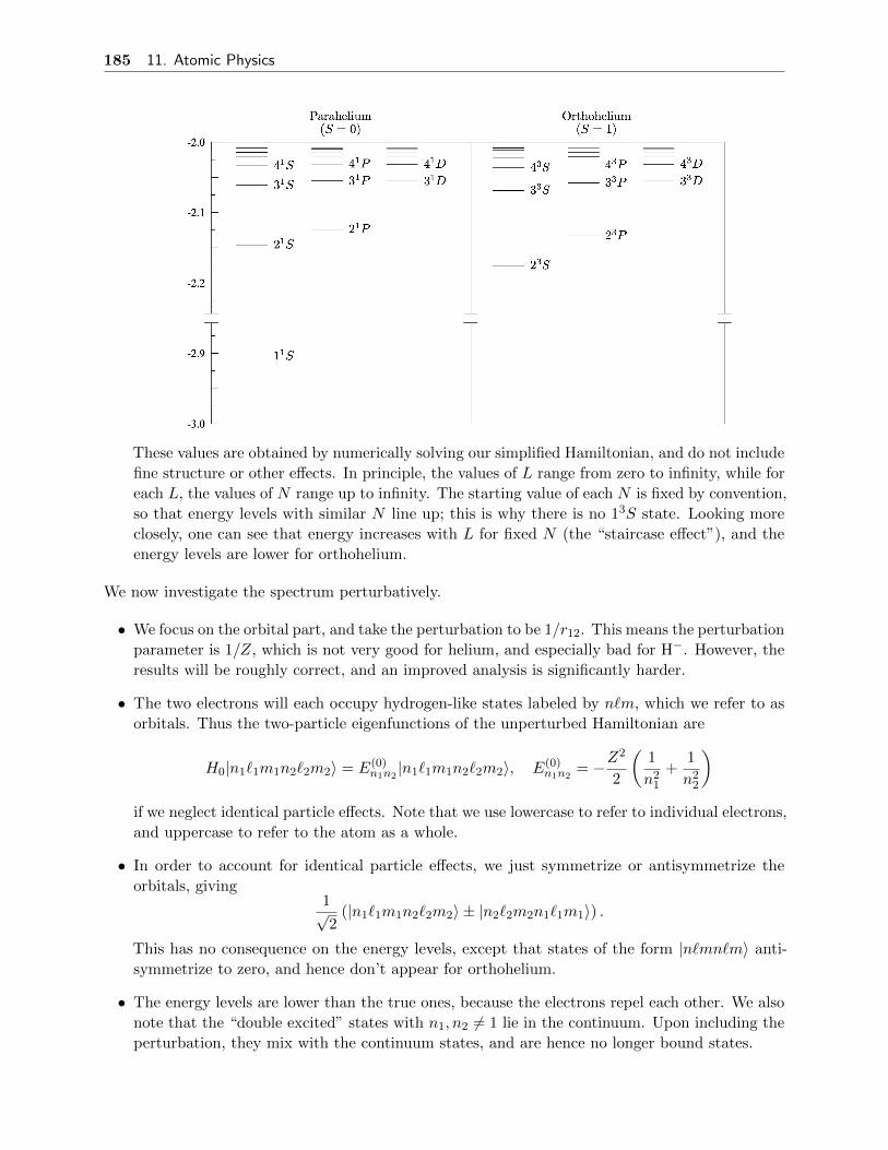
185 11. Atomic Physics
These values are obtained by numerically solving our simplified Hamiltonian, and do not include
fine structure or other effects. In principle, the values of L range from zero to infinity, while for
each L, the values of N range up to infinity. The starting value of each N is fixed by convention,
so that energy levels with similar N line up; this is why there is no 13S state. Looking more
closely, one can see that energy increases with L for fixed N (the “staircase effect”), and the
energy levels are lower for orthohelium.
We now investigate the spectrum perturbatively.
• We focus on the orbital part, and take the perturbation to be 1/r12. This means the perturbation
parameter is 1/Z, which is not very good for helium, and especially bad for H−. However, the
results will be roughly correct, and an improved analysis is significantly harder.
• The two electrons will each occupy hydrogen-like states labeled by n`m, which we refer to as
orbitals. Thus the two-particle eigenfunctions of the unperturbed Hamiltonian are
H0|n1`1m1n2`2m2〉 = E(0)n1n2|n1`1m1n2`2m2〉, E(0)
n1n2= −Z
2
2
(1
n21
+1
n22
)if we neglect identical particle effects. Note that we use lowercase to refer to individual electrons,
and uppercase to refer to the atom as a whole.
• In order to account for identical particle effects, we just symmetrize or antisymmetrize the
orbitals, giving1√2
(|n1`1m1n2`2m2〉 ± |n2`2m2n1`1m1〉) .
This has no consequence on the energy levels, except that states of the form |n`mn`m〉 anti-
symmetrize to zero, and hence don’t appear for orthohelium.
• The energy levels are lower than the true ones, because the electrons repel each other. We also
note that the “double excited” states with n1, n2 6= 1 lie in the continuum. Upon including the
perturbation, they mix with the continuum states, and are hence no longer bound states.

186 11. Atomic Physics
• However, the doubly excited states can be interpreted as resonances. A resonance is a state
that is approximately an energy eigenstate, but whose amplitude “leaks away” over time into
continuum states. For example, when He in the ground state is bombarded with photons, there
is a peak in absorption at energies corresponding to resonances.
• We can get some intuition by semiclassical thinking. We imagine that a photon excites both
electrons to higher orbits. It is then energetically possible for one electron to hit the other,
causing it to be ejected and falling into the n = 1 state in the process. Depending on the
quantum numbers involved, this could take a long time. There is hence an absorption peak at
the resonance, because at short timescales it behaves just like a bound state.
• A similar classical situation occurs in the solar system. It is energetically possible for Jupiter
to eject all of the other planets, at the cost of moving slightly closer to the Sun. In fact,
considerations from chaos theory suggest that over a long enough timescale, this will almost
certainly occur. This timescale, however, is long enough that we can ignore this process and
think of the solar system as a bound object.
• As another example, in Auger spectroscopy, one removes an inner electron by an atom by
collision with a high-speed electron. When an outer shell electron falls into the now empty
state, a photon could be emitted. An alternative possibility is that a different outer electron is
simultaneously ejected; this is the Auger process.
• Now we focus on the true bound states, which are at most singly excited. These are characterized
by a single number n,
E(0)1n = −Z
2
2
(1 +
1
n2
)and can be written as
|NLM±〉 =1√2
(|100n`m〉 ± |n`m100〉)
where N = n, L = `, and M = m. We see there is no N = 1 state for orthohelium.
• The unperturbed energy levels are rather far off. For helium, the unperturbed ground state has
energy −4, while the real answer is about −2.9. For H−, we get −1, while the real answer is
about −0.53.
We now compute the effect of the perturbation.
• The energy shift of the ground state is
∆E = 〈100100|H1|100100〉 =
∫dx1dx2
|ψ100(x1)|2|ψ100(x2)|2
r12
and is equal to the expected energy due to electrostatic repulsion between two 1s electrons.
• The hydrogen-like orbital for the ground state is
ψ100(x) =
(Z3
π
)1/2
e−Zr.

187 11. Atomic Physics
The 1/r12 factor can be expanded as
1
r12=
1
|x1 − x2|=
∞∑`=0
r`<
r`+1>
P`(cos γ)
where r< and r> are the lesser and greater of r1 and r2, and γ is the angle between x1 and x2.
We expand the Legendre polynomial in terms of spherical harmonics with the addition theorem,
P`(cos γ) =4π
2`+ 1
∑m
Y`m(Ω1)Y ∗`m(Ω2).
• Plugging everything in and working in spherical coordinates, we have
∆E =Z6
π2
∫r2
1 dr1
∫dΩ1
∫r2
2 dr2
∫dΩ2 e
−2Z(r1+r2)∞∑`=0
r`<
r`+1>
4π
2`+ 1
∑m
Y`m(Ω1)Y ∗`m(Ω2).
This has the benefit that the angular integrals can be done with the orthonormality of spherical
harmonics. We have∫dΩY`m(Ω) =
√4π
∫dΩY`m(Ω)Y ∗00(Ω) =
√4π δ`0δm0.
This leaves nothing but the radial integrals,
∆E = 16Z6
∫ ∞0
r21 dr1
∫ ∞0
r22 dr2
e−2Z(r1+r2)
r>=
5
8Z
after some tedious algebra. This is one factor of Z down from the unperturbed result −Z2, so
as expected the series is in Z.
• The negatives of the ground state energies for H− and He are hence
zeroth order : 1, 4, first order : 0.375, 2.75, exact : 0.528, 2.904
which are a significant improvement, though the first order correction overshoots. Indeed, as
mentioned earlier, the first order result always overestimates the ground state energy by the
variational principle, and hence sets an upper bound. It is trickier to set a lower bound, though
at the very least the zeroth order result serves as one, since it omits a repulsive interaction.
• To show H− has a bound state, we must show that the ground state energy is below the
continuum threshold of −0.5. Unfortunately, our result of −0.375 is not quite strong enough.
We now compute the first-order energy shift for the excited states.
• As stated earlier, we only need to consider singly excited states, namely the states |NLM±〉defined above for N > 1. The energy shift is
∆ENL± = 〈NLM±|H1|NLM±〉
where there is no dependence on M because H1 is a scalar operator.
188 11. Atomic Physics
• Expanding the definition of |NLM±〉, we have four terms,
∆ENL± =1
2
(〈100n`m|H1|100n`m〉+ 〈n`m 100|H1|n`m 100〉
± (〈100n`m|H1|n`m 100〉+ |n`m 100〉H1|100n`m〉)).
The first two terms are equal, as are the last two, so
∆ENL± = Jn` ±Kn`, Jn` = 〈100n`m| 1
r12|100n`m〉, Kn` = 〈100n`m| 1
r12|n`m 100〉.
The corresponding two integrals are called the direct and exchange integrals, respectively.
• The direct integral has the simple interpretation of the mutual electrostatic energy of the two
electron clouds,
Jn` =
∫dx1dx2
|ψ100(x1)|2|ψn`m(x2)|2
|x1 − x2|.
It is clearly real and positive.
• The exchange integral is
Kn` =
∫dx1dx2
ψ∗100(x1)ψ∗n`m(x2)ψn`m(x1)ψ100(x2)
|x1 − x2|.
This is real, as swapping the variables of integration conjugates it, but also keeps it the same.
It can be shown, with some effort, that the exchange integrals are positive; this is intuitive,
since the denominator goes to zero when x1 ≈ x2, and in such regions the numerator is positive
(i.e. has a small phase).
• The fact that Kn` is positive means that the ortho states are lower in energy than the para
states. Intuitively this is because the ortho wavefunctions vanish when x1 = x2, while the para
wavefunctions have maxima/nodes at x1 = x2. Hence the ortho states have less electrostatic
repulsion.
• Another important qualitative features is that the direct integrals Jn` increase with `, leading
to the “staircase effect” mentioned earlier. As for the alkali atoms, this is intuitively because as
the angular momentum of one electron is increased, it can move further away from the nucleus,
and the nuclear charge is more effectively screened by the other electron(s).
We have hence explained all the qualitative features of the spectrum, though perturbation theory
doesn’t do very well quantitatively. We can do a bit better using the variational principle.
• We recall that the unperturbed ground state just consists of two 1s electrons, which we refer
to as 1s2, with wavefunction
Ψ1s2(x1,x2) =Z3
πe−Z(r1+r2).
However, we also know that each electron partially screens the nucleus from the other, so each
electron sees an effective nuclear charge Ze between Z − 1 and Z. This motivates the trial
wavefunction
Ψ(x1,x2) =Z3e
πe−Ze(r1+r2)
where Ze is a variational parameter.
189 11. Atomic Physics
• To evaluate the expectation value of H, we write it as
H =
(p2
1
2− Zer1
)+
(p2
2
2− Zer2
)+ (Ze − Z)
(1
r1+
1
r2
)+
1
r12.
This has the advantage that the first two terms are both clearly equal to −Z2e/2.
• The third term gives
2(Ze − Z)
∫dx
Z3e
π
e−Zer
r= 2(Ze − Z)Ze.
Finally, the last term is just one we computed above but with Z replaced with Ze, and is hence
equal to (5/8)Ze.
• Adding up the pieces, the variational energy is
E(Ze) = Z2e − 2ZZe +
5
8Ze
which is minimized for
Ze = Z − 5
16.
That is, each electron screens 5/16 of a nuclear charge from the other electron.
• The variational estimate for the ground state energy is hence
Evar = −Z2 +5
8Z − 25
256=
−0.473 H−
−2.848 He.
This is closer than our result from first-order perturbation theory. However, since the estimate
for H− is still not below −0.5, it isn’t enough to prove existence of the bound state. This can
be done by using a more sophisticated ansatz; our was very crude, not even accounting for the
fact that the electrons should preferentially be on opposite sides of the nucleus.
11.3 The Thomas–Fermi Model
In this section we introduce the Thomas–Fermi model, a crude model for multi-electron atoms.
• The idea of the model is to represent the electron cloud surrounding the nucleus as a zero tem-
perature, charged, degenerate Fermi–Dirac fluid, in hydrostatic equilibrium between degeneracy
pressure and electrostatic forces.
• The results we need from statistical mechanics are that for zero-temperature electrons in a
rectangular box of volume V with number density n, the Fermi wavenumber is
kF = (3π2n)1/3
and the total energy is
E =~2V k5
F
10mπ2=
~2(3π2N)5/3
10mπ2V −2/3.
Deriving these results is straightforward, remembering to add a factor of 2 for electron spin.
190 11. Atomic Physics
• As usual, the pressure is a derivative of energy,
P = −dEdV
=~2
15mπ2(3π2n)5/3.
We note that P is written solely in terms of constants and n. The key to the Thomas–Fermi is
to allow n to vary in space, and treat the electrons as a fluid with pressure P (n(x)). Of course,
this is precisely valid only in the thermodynamic limit.
• If Φ is the electrostatic potential, then in hydrostatic equilibrium,
∇P = en∇Φ
where e > 0. Furthermore, Φ obeys Poisson’s equation,
∇2Φ = −4πρ = 4πne− 4πZeδ(x)
in Gaussian units, where we included the charge density for the nucleus explicitly. We will drop
this term below and incorporate it in the boundary conditions at r = 0.
• We take P , n, and Φ to depend only on r. Now, we have
∇P =~2
3m(3π2)2/3n2/3∇n
and plugging this into the hydrostatic equilibrium equation gives
~2
3m(3π2)2/3n−1/3∇n = e∇Φ.
We may integrate both sides to obtain
~2
2m(3π2n)2/3 = e(Φ− Φ0) ≡ eΨ.
• To get intuition for this equation, we note that it can be rewritten as
p2F
2m− eΦ = −eΦ0.
The left-hand side is the energy of an electron at the top of the local Fermi sea, so evidently
this result tells us it is a constant, the chemical potential of the gas. This makes sense, as in
equilibrium these electrons shouldn’t have an energetic preference for being in any one location
over any other.
• We know the potential must look like
Φ(r) ∼
Ze/r r → 0,
0 r →∞.
It is intuitively clear that as we move outward, the potential energy goes up monotonically and
the kinetic energy goes down.
• The behavior of the potential is different depending on the number of electrons N .

191 11. Atomic Physics
– If N > Z, we have a negative ion. Such atoms can’t be described by the Thomas-Fermi
model, because ∇P always points outward, while at some radius the electrostatic force will
start pointing outward as well, making the hydrostatic equilibrium equation impossible to
satisfy. In this model, the extra negative charge just falls off.
– If N = Z, we have a neutral atom. Then Φ(r) falls off faster than 1/r. Such a case is
described by Φ0 = 0.
– If N < Z, we have a positive ion, so Φ(r) falls off as (Z −N)e/r. Such a case is described
by Φ0 > 0. At some radius r0, the kinetic energy and hence n falls to zero. Negative values
are not meaningful, so for all r > r0 the density is simply zero.
– The case Φ0 < 0 also has physical meaning, and corresponds to a neutral atom under
applied pressure.
We now solve the model more explicitly.
• In terms of the variable Ψ, we have
~2
2m(3π2n)2/3 = eΨ, ∇2Ψ = 4πne.
We eliminate n to solve for Ψ. However, since we also know that Ψ ∼ Ze/r for small r, it is
useful to define the dimensionless variable
f(r) =rΨ(r)
Ze, f(0) = 1.
• Doing a little algebra, we find the Thomas–Fermi equation
d2f
dx2=f3/2
x1/2, r = bx, b =
(3π)2/3
27/3
a0
Z1/3
where x is a dimensionless radial variable.
• Since f(0) is already set, the solutions to the equation are parametrized by f ′(0). Some numeric
solutions are shown below.
The case f ′(0) = −1.588 corresponds to a neutral atom. The density only approaches zero
asymptotically. It is a universal function that is the same, up to scaling, for all neutral atoms
in this model.
• As the initial slope becomes more negative, the density reaches zero at finite radius, correspond-
ing to a positive ion with a definite radius.
192 11. Atomic Physics
• When the initial slope is less negative, the density never falls to zero. Instead, we can manually
cut it off at some radius and just declare the density is zero outside this radius, which physically
translates to imposing an external pressure. This is only useful for modeling neutral atoms
(with neutrality determining where the cutoff radius is) since one cannot collect a bulk sample
of charged ions.
• The Thomas-Fermi model has obvious limitations. For example, by treating the electrons as
a continuous fluid, we lose all shell structure. In general, the model is only reasonable for
describing the electron density at intermediate radii, breaking down both near the nucleus and
far from it.
• It can be used to calculate average properties, such as the average binding energy of charge
radius, which make it useful in experimental physics, e.g. for calculations of the slowing down
of particles passing through matter.
11.4 The Hartree–Fock Method
The Hartree–Fock method is a variational method for approximating the solution of many-body
problems in atoms, molecules, solids, and even nuclei. We begin with the simpler Hartree method.
• We consider an atom with N electrons and nuclear charge Z, and use the basic Hamiltonian
H =N∑i=1
(p2i
2− Z
ri
)+∑i<j
1
rij≡ H1 +H2.
This neglects effects from the finite nuclear mass, fine and hyperfine structure, retardation,
radiative corrections, and so on. In particular, fine structure becomes more important for
heavier atoms, since it scales as (Zα)2, and in these cases it is better to start from the Dirac
equation. Also note that the electron spin plays no role in the Hamiltonian.
• The Hamiltonian commutes with the total orbital angular momentum L, as well as each of
the individual spin operators Si. It also commutes with parity π, as well as all the exchange
operators Eij .
• This is our first situation with more than 2 identical particles, so we note that exchanges
generate all permutations. For each permutation P ∈ SN , there is a unitary permutation
operator U(P ) which commutes with the Hamiltonian, and which we hereafter just denote by
P . We denote the sign of P by (−1)P .
• In general, the symmetrization postulate states that allowed states satisfy
P |Ψ〉 =
|Ψ〉 bosons,
(−1)P |Ψ〉 fermions.
All physically meaningful operators must commute with the U(P ). If one begins with a formal
Hilbert space that doesn’t account for the symmetrization postulate, then one can project onto
the fermionic subspace with
A =1
N !
∑P
(−1)PP.
We will investigate such projectors in more detail in the notes on Group Theory.

193 11. Atomic Physics
We now describe Hartree’s trial wavefunction.
• In Hartree’s basic ansatz, we simply ignore the symmetrization postulate. We take a trial
wavefunction of the form
|ΦH〉 = |1〉(1) . . . |N〉(N)
where the individual terms are single particle orbitals, describing the state of one electron. The
notation is a bit ambiguous: here Latin indices in parentheses label the electrons while Greek
indices in the kets label the orbitals.
• The orbitals are assumed to be normalized, and the product of a spatial and spin part,
|λ〉 = |uλ〉|msλ〉
where |msλ〉 is assumed to be an eigenstate of Sz with eigenvalue msλ = ±1/2. This causes no
loss of generality, because the Hamiltonian has no spin dependence.
• The variational parameters are, in principle, the entire spatial wavefunctions of the orbitals
uλ(r). It is straightforward to compute the expectation of H1,
〈ΦH |H1|ΦH〉 =
N∑λ=i=1
〈λ|(i)hi|λ〉(i), hi =p2i
2− Z
ri
where the other bras and kets collapse by normalization. Explicitly, the expectation is
〈ΦH |H1|ΦH〉 =∑λ
Iλ, Iλ =
∫dru∗λ(r)
(p2
2− Z
r
)uλ(r).
• The expectation of H2 gives a sum over pairs,
〈ΦH |H2|ΦH〉 =∑
λ=i<µ=j
〈λ|(i)〈µ|(j) 1
rij|λ〉(i)|µ〉(j).
Explicitly, this is a sum of direct integrals,
〈ΦH |H2|ΦH〉 =∑λ<µ
Jλµ, Jλµ =
∫dridrj u
∗λ(ri)u
∗µ(rj)
1
rijuλ(ri)uµ(rj).
No exchange integrals have appeared, since we haven’t antisymmetrized. We are dropping the
self-interaction term λ = µ since we dropped the i = j term in the original Hamiltonian. This
term was dropped classically to avoid infinite self-energy for point charges, though note that in
this quantum context, Jλλ actually need not be divergent.
• Using the symmetry of the direct integrals, the energy functional is
E[ΦH ] = 〈ΦH |H|ΦH〉 =∑λ
Iλ +1
2
∑λ 6=µ
Jλµ.
However, we can’t just minimize this directly; as usual we need a Lagrange multiplier to enforce
normalization, so we instead minimize
F [ΦH ] = E[ΦH ]−∑λ
ελ(〈λ|λ〉 − 1).
194 11. Atomic Physics
• The vanishing of the functional derivative δF/δuλ(r) gives the Hartree equations(p2
2− Z
r
)uλ(r) + Vλ(r)uλ(r) = ελuλ(r), Vλ(r) =
∑µ6=λ
∫dr′|uµ(r)|2
|r− r′|.
These equations have a simple interpretation. We see that each electron obeys a Schrodinger
equation with energy ελ, and feels a potential sourced by the average field of the other charges,
which makes the equations an example of a mean field theory.
• This is a set of N coupled, nonlinear, integro-differential equations. Sometimes one speaks of
the self-consistent field, since the field determines the orbitals and vice versa.
• In practice, one solves the Hartree equations by iteration. For example, one can begin by
computing the Thomas–Fermi potential, then setting the initial guess for the orbitals to be
the eigenfunctions of this potential. Then the new potentials are computed, and the resulting
Schrodinger equation is solved, and so on until convergence.
• The computationally expensive part is solving the three-dimensional Schrodinger equations.
Hartree suggested further replacing the potential with a central potential
Vλ(r) =1
4π
∫dΩVλ(r).
Then the Schrodinger equation reduces to a radial equation, which is much easier to solve. This
is a reasonable step if we expect the atom to be nearly spherically symmetric overall.
• Since the Hartree orbitals are eigenfunctions of different Schrodinger equations, there is no need
for them to be orthogonal.
• It is tempting to think of ελ as the “energy of each electron”, but this is misleading because
each electron’s Hartree equation counts the interaction with every other electron. That is, if
we just summed up all the ελ, we would not get the total energy because the interaction would
be double counted.
• More explicitly, if we multiply the Hartree equation by u∗λ(r) and integrate,
Iλ +∑µ6=λ
Jλµ = ελ
and summing gives
E[ΦH ] =∑λ
ελ −1
2
∑λ 6=µ
Jλµ.
Next, we consider Fock’s refinement to Hartree’s wavefunction.
• Fock’s trial wavefunction is just a fully antisymmetrized version of Hartree’s,
|Φ〉 =√N !A|ΦH〉 =
1√N !
∣∣∣∣∣∣∣∣∣|1〉(1) |2〉(1) . . . |N〉(1)
|1〉(2) |2〉(2) . . . |N〉(2)
......
. . ....
|1〉(N) |2〉(N) . . . |N〉(N)
∣∣∣∣∣∣∣∣∣ .

195 11. Atomic Physics
This second way of writing the wavefunction is known as a Slater determinant, and is expanded
like a regular determinant with scalar multiplication replaced with tensor product. The rest of
the idea is the same: we simply variationally minimize the energy.
• Note that the Slater determinant vanishes if the N orbitals are not linearly independent. Mean-
while, if they are linearly independent, then they span an N -dimensional subspace of the
single-particle Hilbert space, and up to scaling the Slater determinant only depends on what
this subspace is. Hence, unlike in Hartree’s wavefunction, we can always choose the orbitals to
be orthonormal without loss of generality, in which case |Φ〉 is automatically normalized.
• We have to make a point about language. We often speak of a particle being “in” a single-
particle state |λ〉 (such as the Pauli exclusion principle’s “two particles can’t be in the same
state”). But because of the antisymmetrization, what we actually mean is that the joint state
is a Slater determinant over a subspace containing |λ〉.
• However, even though Slater determinants are very useful, they are not the most general valid
states! For instance, the superposition of two such states is generally not a Slater determinant.
Accordingly, the Hartree–Fock trial wavefunction doesn’t generally get the exact answer. In
such cases it really is not valid to speak of any individual particle as being “in” a state. Even
saying “the electrons fill the 1s and 2s orbitals” implicitly assumes a Slater determinant and is
not generally valid, but we use such language anyway because of the great difficulty of going
beyond Hartree–Fock theory.
• To evaluate the energy functional, we note that A commutes with H, since the latter is a
physical operator, so
〈Φ|H|Φ〉 = N !〈ΦH |A†HA|ΦH〉 = N !〈ΦH |HA2|ΦH〉 = N !〈ΦH |HA|ΦH〉 =∑P
(−1)P 〈ΦH |HP |ΦH〉.
Of course, the same reasoning holds for H1 and H2 individually.
• Now consider the expectation of H1 =∑
i hi. The expectation of each hi vanishes by orthogo-
nality unless P fixes all j 6= i. But this means only the identity permutation contributes. Hence
the sum over permutations does nothing, and the result is the same as in Hartree theory.
• Next, consider the expectation of H2 =∑
i<j 1/rij . By the same reasoning, the contribution of
the term 1/rij vanishes except for permutations that fix everything besides i and j, of which
there are only the identity permutation and the exchange Eij .
• The latter gives an exchange integral, so
〈Φ|H2|Φ〉 =∑λ<µ
Jλµ −Kλµ, Kλµ = δ(msλ,msµ)
∫drdr′
u∗λ(r)u∗µ(r′)uλ(r′)uµ(r)
|r− r′|
as we saw for helium. Note that the exchange integrals, unlike the direct integrals, depend
on the spin. As for helium, one can show the exchange integrals are positive. Since they
contribute with a minus sign, they lower the energy functional, confirming the expectation that
Hartree–Fock theory gives a better estimate of the ground state energy than Hartree theory.
196 11. Atomic Physics
• Again as we saw for helium, the lowering is only in effect for aligned spins, as this corresponds
to antisymmetry in the spatial wavefunction. This leads to Hund’s first rule, which is that
electrons try to align their spins. Half-filled electron shells are especially stable, since all the
electrons are aligned, leading to, e.g. the high ionization energy of nitrogen. It also explains
why chromium has configuration 3d54s instead of 3d44s2 as predicted by the aufbau principle.
• Another way in which Hartree–Fock theory makes more sense is that the self-energy, if included,
ultimately cancels out because Jλλ = Kλλ. Hence we can include it, giving
〈Φ|H2|Φ〉 =1
2
∑λµ
Jλµ −Kλµ.
As we’ll see, including the self-energy makes the final equations nicer as well.
Finally, we minimize the Hartree–Fock energy.
• The functional to be minimized is
F [Φ] =∑λ
Iλ +1
2
∑λµ
(Jλµ −Kλµ)−∑λ
ελ(〈λ|λ〉 − 1).
Note that we are only enforcing normalization with Lagrange multipliers; we will see below that
we automatically get orthogonality.
• Carrying out the functional derivative, we find the Hartree–Fock equations(p2
2− Z
r
)uλ(r) + Vd(r)uλ(r)−
∫dr′ Vex(r, r′)uλ(r′) = ελuλ(r)
where the direct and exchange potentials are
Vd(r) =∑µ
∫dr′|uµ(r′)|2
|r− r′|, Vex(r, r′) =
∑µ
δ(msλ,msµ)uµ(r)u∗µ(r′)
|r− r′|.
Since we included the self-energy contributions, all electrons feel the same direct potential.
• The exchange potential is a bit harder to interpret, as it is a nonlocal operator. However, we
note that there are only two distinct exchange potentials because ms can only have two values,
V ±ex (r, r′) =∑µ
δ(msµ,±1/2)uµ(r)u∗µ(r′)
|r− r′|.
Hence all spin up and spin down orbitals experience V +ex and V −ex respectively.
• As such, the Hartree–Fock equations can be thought of as just two coupled Schrodinger-like
equations, one for each spin. The solutions are automatically orthogonal, because orbitals of
different spins are orthogonal, while orbitals of the same spin are eigenfunctions of the same
Hamiltonian. This illustrates how Hartree–Fock theory is more elegant than Hartree theory.
• The main disadvantage of Hartree–Fock theory is numerically handling the nonlocal potential,
and there are many clever schemes to simplify dealing with it.
197 11. Atomic Physics
• Integrating the Hartree–Fock equation against uλ(r)∗ gives
Iλ +∑µ
(Jλµ −Kλµ) = ελ.
As before, the energies ελ double count the interaction,∑λ
ελ = E +1
2
∑λµ
(Jλµ −Kλµ).
• On the other hand, note that if we remove the electron with the highest associated ελ, chosen
to be εN , we can write the energy of the remaining electrons as
E′ =N−1∑λ=1
I ′λ +1
2
N−1∑λ,µ=1
(J ′λµ −K ′λµ).
If we assume the self-consistent fields have not been significantly changed, so that I ′ = I, J ′ = J
and K ′ = K, then we have an expression for the ionization potential,
E − E′ = εN .
This is Koopman’s theorem.
• To simplify calculations, we can average the potentials over angles just as in Hartree theory.
This is a little trickier to write down explicitly for the nonlocal potential, but corresponds to
replacing V ±ex(r, r′) with an appropriately weighted average of U(R)V ±exU(R)† for R ∈ SO(3),
where the U(R) rotates space but not spin. The resulting averaged potential can only depend
on the rotational invariants of two vectors, namely |r|2, |r′|2, and r · r′.
• A further approximation is to average over spins, replacing the two exchange potentials V ±ex
with their average. In this case, we have reduced the problem to an ordinary central force
problem, albeit with a self-consistent potential, and we can label its orbitals as |n`m`ms〉. This
is what people mean, for example, when they say that the ground state of sodium is 1s22s22p63s.
However, this level of approximation also erases, e.g. the tendency of valence electrons to align
their spins, which must be put in manually.
11.5 Atomic Structure
We now apply Hartree–Fock theory to atomic structure, assuming rotational averaging throughout.
• The Hartree–Fock method gives a variational ansatz for the ground state of the basic Hamiltonian
H =∑i
(p2i
2− Z
ri
)+∑i<j
1
rij.
The resulting states in the Slater determinant are solutions of the Schrodinger-like equation
huλ(r) = ελuλ(r), h(r,p) =p2
2− Z
r+ V d − V ex.
Note that numerically, everything about a Hartree–Fock solution can be specified by the Rn`(r)
and εn`, since these can be used to infer the potentials.
198 11. Atomic Physics
• Hartree–Fock theory gives us the exact ground state to the so-called central field approximation
to the Hamiltonian,
H0 =∑i
h(ri,pi).
Thus, we can treat this as the unperturbed Hamiltonian and the error as a perturbation,
H = H0 +H1, H1 =∑i<j
1
rij−∑i
(V d,i − V ex,i
).
The term H1 is called the residual Coulomb potential, and the benefit of using Hartree–Fock
theory is that H1 may be much smaller than just∑
i<j 1/rij alone.
• The unperturbed Hamiltonian H0 is highly symmetrical; for example, it commutes with the
individual Li and Si of the electrons. (Here and below, the potentials in H0 are regarded as
fixed; they are always equal to whatever they were in the Hartree–Fock ground state.) Therefore,
the useful quantum numbers depend on the most important perturbations.
• If H1 is the dominant perturbation, then we recover the basic Hamiltonian H0, for which L
and S are good quantum numbers; as usual capital letters denote properties of the atom as a
whole. This is known as LS or Russell–Saunders coupling.
• Fine structure gives the additional perturbation
H2 ∼∑i
Li · Si
which instead favors the so-called jj-coupling. Fine structure is more important for heavier
atoms, so for simplicity we will only consider lighter atoms, and hence only LS coupling.
• Now we consider the degeneracies in H0. The energy only depends on the n` values of the
occupied states. In general, a state can be specified by a set of completely filled orbitals, plus a
list of partly filled orbitals, along with the (m`,ms) values of the states filled in these orbitals.
We call this data an m-set, or electron configuration.
• For the ground states of the lightest atoms, only at most one orbital will be partly filled. If it
contains n electrons, then the degeneracy is(2(2`+ 1)
n
).
In the case of multiple partly filled orbitals, we would get a product of such factors.
• Now, the relevant operators that commute with H are L2, Lz, S2, Sz, and π. Hence in LS
coupling we can write the states as |γLSMLMS〉, where γ is an index for degenerate multiplets;
these start appearing at Z = 23. The energy depends only on the L and S values.
• The Slater determinants are eigenstates of some of these operators,
Lz|m-set〉 = ML|m-set〉, Sz|m-set〉 = MS |m-set〉, π|m-set〉 =∏i
(−1)`i |m-set〉
where
ML =∑i
m`i, MS =∑i
msi.
199 11. Atomic Physics
The sums range over all of the electrons, but can be taken to range over only unfilled orbitals
since filled ones contribute nothing.
• However, the Slater determinants are not eigenstates of L2 and S2. Computing the coefficients
that link the |m-set〉 and |LSMLMS〉 bases is somewhat complicated, so we won’t do it in
detail. (It is more than using Clebsch–Gordan coefficients, because there can be more than two
electrons in the m-set, and we need to keep track of both orbital and spin angular momentum
as well as the antisymmetrization.) Instead, we will simply determine which values of L and S
appear, for a given electron configuration. Note that the parity does not come into play here,
since all states for a given electron configuration have the same parity.
• As for helium, we label these multiplets as 2S+1L. The spin-orbit coupling splits the multiplets
apart based on their J eigenvalue, so when we account for it, we write 2S+1LJ . Also, for clarity
we can also write which electron configuration a given multiplet comes from, 2S+1L....
• Finally, once we account for the spin-orbit coupling, we can also account for the Zeeman effect,
provided that it is weaker than even the spin-orbit coupling. In this case, the procedure runs
exactly as for a hydrogen atom with fine structure, and Lande g-factors appear after applying
the projection theorem.
We now give a few examples, focusing on the ground states of H0 for simplicity.
Example. Boron. The ground states of H0 have an electron configuration 1s22s22p, with a
degeneracy of 6. Since there is only one relevant electron, there is clearly one multiplet 2P , where
L = ` = 1 and S = s = 1/2.
Example. Carbon. We start with the electron configuration 1s22s22p2, which has degeneracy(62
)= 15. Now, since there are only two relevant electrons, we can have L = 0, 1, 2 and S = 0, 1,
with each L value represented once. Overall antisymmetry determines the S values, giving 1S, 3P ,
and 1D. These have dimensions 1, 9, and 5, which add up to 15 as expected.
Some of the low-lying atomic energy levels for carbon are shown below, where the energy is
measured in eV.

200 11. Atomic Physics
The electron configurations shown here are
a = 2p2, b = 2p3p, c = 2p3d, d = 2p4p, e = 2s2p3, f = 2p3s, g = 2p4s
where 1s22s2 is implicit except in e.
The lowest energy multiplet can be determined heuristically using the aufbau principle and Hund’s
rules, which are covered in the notes on Solid State Physics. For example, consistent with the aufbau
principle, the a = 2s22p2 configurations are all below the e = 2s2p3 configuration; evidently the 2s
state is lower in energy because it can penetrate the shielding. Within the a = 2s22p2 configuration,
we have three multiplets, and Hund’s rules account for their energy ordering.
The first two of Hund’s rules account for the details of the exchange force, neglected in H0. For
carbon, Hund’s first rule shows that 3P a has the lowest energy. Hund’s third rule accounts for the
spin-orbit interaction, which is subdominant in this case; it can be used to determine the lowest
energy state within the 3P a multiplet. Concretely this would be done by switching to the coupled
basis, just as for hydrogen, at which point one finds the ground state is 3P a0 .
For atoms of higher Z, the splittings associated with Hund’s rules become larger; when they are
comparable to the splittings in H0 itself, exceptions to the aufbau principle occur.
Example. Nitrogen. We start with the electron configuration 1s22s22p3, which has degeneracy(63
)= 20. This requires a more systematic approach. The general approach is like that of Clebsch–
Gordan decomposition. We sort the states by the (ML,MS) values. A highest pair (i.e. a state
annihilated by L+ and S+) must be the doubly stretched/highest weight state of a 2S+1L multiplet.
We then cross out the other (ML,MS) values in this multiplet and repeat the process. Furthermore,
since we’re focusing on highest weight states, we need only consider states with ML,MS ≥ 0.
In this case, the relevant (ML,MS) values are
1× (2, 1/2), 2× (1, 1/2), 1× (0, 3/2), 3× (0, 1/2)
201 11. Atomic Physics
where the prefactor indicates the multiplicity. The first state is hence the highest weight state of a2D multiplet. Crossing this multiplet out leaves
1× (1, 1/2), 1× (0, 3/2), 2× (0, 1/2).
The first state left over is the highest weight state of a 2P multiplet. Finally we are left with a 4S
multiplet. The dimensions are 10 + 6 + 4, which add up to 20 as expected.
Example. Oxygen. The electron configuration is 1s22s22p4. This is actually easier than nitrogen
because we can treat the two missing electrons as “holes”, with the same ` and s but opposite m`
and ms from an electron. The LS multiplets are hence exactly the same as in carbon.
Note. The first case in which the ground state of H0 yields degenerate LS multiplets is the case
of three d electrons, which first occurs for Vanadium, Z = 23. For anything more complicated than
this, the answer is rather tedious to work out, and one consults standard tables.
11.6 Chemistry
202 12. Time Dependent Perturbation Theory
12 Time Dependent Perturbation Theory
12.1 Interaction Picture
We begin with the basics of interaction picture.
• In time-dependent perturbation theory, we consider the Hamiltonian
H(t) = H0 +H1(t)
where H0 is solvable and H1 is treated as a perturbation.
• We are interested in calculating the transition amplitudes
〈f |U(t)|i〉
where typically |i〉 and |f〉 are two eigenstates of the unperturbed Hamiltonian, and U(t) is the
time evolution operator. It’s useful to do this in the interaction picture.
• In Heisenberg picture, we transfer all time-dependence to the operators, so
AH(t) = U †(t)AS(t)U(t)
where U(t) is the time evolution operator for H(t) from 0 to t. The states are ‘frozen’ at time
t = 0. Then all expectation values come out the same as in Schrodinger picture.
• If CS = ASBS , then CH = AHBH . As a result, all operator identities remain true in Heisenberg
picture, including commutation relations.
• In particular, the expression for the Hamiltonian remains valid, so
HH(t) = HS(pH(t), xH(t), t).
In the special case [HS(t), HS(t′)] = 0 for all times (e.g. when it is time-independent) we find
HH(t) = HS(t).
• Differentiating the Heisenberg operator definition and using
i~∂U(t)
∂t= HS(t)U(t)
we find the Heisenberg equation of motion,
i~dAH(t)
dt= [AH(t), HH(t)] + i~
(∂AS(t)
∂t
)H
.
• Time-independent Schrodinger operators that always commute with the Hamiltonian are said
to be ‘conserved’ in Schrodinger picture; in Heisenberg picture, they have no time evolution.

203 12. Time Dependent Perturbation Theory
Example. The harmonic oscillator. Setting all constants to one,
HS =p2S + x2
S
2.
Since the Hamiltonian is time-independent, HS = HH . To check this, note that
HH =p2H + x2
H
2=
(p2S + x2
S)(cos2 t+ sin2 t)
2= HS
where we plugged in the known time dependence of pH and xH .
Now we turn to the interaction picture. We leave S subscripts implicit.
• Let U0(t) be the time evolution due to just H0, so
i~∂U0(t)
∂t= H0U0(t)
In the interaction picture, we ‘cancel out’ the state evolution due to H0, defining
|ψI(t)〉 = U †0(t)|ψS(t)〉, AI(t) = U †0(t)AS(t)U0(t)
with the operator evolution chosen to preserve expectation values.
• Define the time evolution operator in the interaction picture as
|ψI(t)〉 = W (t)|ψI(0)〉.
Combining the above results, we find
W (t) = U0(t)†U(t).
That is, we evolve forward in time according to the exact Hamiltonian, then evolve backward
under the unperturbed Hamiltonian.
• Differentiating and simplifying gives
i~∂W (t)
∂t= H1I(t)W (t)
where H1I(t) is the perturbation term in the interaction picture. Integrating this gives
W (t) = 1 +1
i~
∫ t
0dt′H1I(t
′)W (t′)
and plugging this equation into itself gives a series solution for W (t), the Dyson series.
• A succinct way to write the full result is by a time-ordered exponential,
W (t) = T exp
(1
i~
∫ t
0dt′H1I(t
′)
).
This is the generic solution to a Schrodinger equation with time-dependent Hamiltonian.
• In general, we can always split the Hamiltonian so that one piece contributes to the time
evolution of the operators (by the Heisenberg equation) and the other contributes to the time
evolution of the states (by the Schrodinger equation). Interaction picture is just the particular
splitting into H0 and H1(t).

204 12. Time Dependent Perturbation Theory
12.2 Fermi’s Golden Rule
For simplicity, we begin with the case where H0 has a discrete spectrum, H0|n〉 = En|n〉, with
initial state |i〉.
• Applying the Dyson series, the interaction picture state at a later time is
|ψI(t)〉 = |i〉+1
i~
∫ t
0dt′H1I(t
′)|i〉+1
(i~)2
∫ t
0dt′∫ t′
0dt′′H1I(t
′)H1I(t′′)|i〉+ · · · .
• Our goal is to calculate the coefficients
|ψI(t)〉 =∑n
cn(t)|n〉.
The cn(t) differ from the transition amplitudes mentioned earlier because they lack the rapidly
oscillating phase factors eiEnt/~; such factors don’t affect transition probabilities. (Note that
the eigenstates |n〉 are the same in all pictures; states evolve in time but eigenstates don’t.)
• Using the Dyson series, we can expand each coefficient in a power series
cn(t) = δni + c(1)n (t) + c(2)
n (t) + . . . .
The first term is
c(1)n (t) =
1
i~
∫ t
0dt′ 〈n|H1I(t
′)|i〉 =1
i~
∫ t
0dt′ eiωnit
′〈n|H1(t′)|i〉, ωni =En − Ei
~
where we converted H1 back to Schrodinger picture.
• Similarly, the second order term is
c(2)n (t) =
1
(i~)2
∫ t
0dt′∫ t′
0dt′′
∑k
eiωnkt′+iωkit
′′〈n|H1(t′)|k〉〈k|H1(t′′)|i〉.
Here, we added a resolution of the identity; the second order term evidently accounts for
transitions through one intermediate state.
• To make further progress, we need to specify more about the perturbation H1. For example,
for a constant perturbation, the phase factors come out of the integral, giving
c(1)n (t) =
2
i~eiωnit/2
sinωnit/2
ωni〈n|H1|i〉.
The corresponding transition frequency, to first order, is
Pn(t) =4
~2
sin2 ωnit/2
ω2ni
|〈n|HI |i〉|2.
We see the probability oscillates sinusoidally in time, to first order.

205 12. Time Dependent Perturbation Theory
Example. The next simplest example is sinusoidal driving. The most general example is
H1(t) = Ke−iω0t +K†eiω0t
where K need not be Hermitian. As a result, the expression for c(1)n has two terms, with denominators
of ωni ± ω0. Therefore, the effect of a sinusoidal driving can be very large when it is on resonance
with a transition. When ωni ≈ ω0, the K term dominates, so we may make the “rotating wave
approximation” and drop K†. We then have
Pn(t) =4
~2
sin2(ωni − ω0)t/2
(ωni − ω0)2|〈n|K|i〉|2.
Physically, this could translate to absorption of light, where a sinusoidal electromagnetic field is the
driving; the response is Lorentzian. Since the K† term must be there as well, we also get resonance
for ωni ≈ −ω0. Physically, that process corresponds to stimulated emission.
Generally, the probability is proportional to 1/(∆ω)2 and initially grows as t2. The probability
can exceed unity close to resonance, signaling that first order perturbation theory breaks down.
Next, we consider the case of a continuum of final states, which yields Fermi’s golden rule.
• Shifting the frequency to be zero on resonance, the total transition probability to all states near
resonance. at first order, is
P (t) ≈ 4
~2
∫ ∞−∞
dωsin2 ωt/2
ω2g(ω)|〈fω|K|i〉|2
where g(ω) is the density of states.
• The function sin2(ωt/2)/ω2 is peaked around |ω| . 1/t to a height of t2/4, so area of the
central lobe is O(t). Away from the lobe, for |ω| & 1/t, we have oscillations of amplitude 1/ω2.
Integrating, the total area of the side lobes also grows as t. We thus expect the total area to
grow as t, and contour integrating shows∫ ∞−∞
dωsin2 ωt/2
ω2=πt
2.
• As t→∞, the integral’s contribution becomes concentrated about ω = 0, so
limt→∞
1
t
sin2 ωt/2
ω2=π
2δ(ω).
More generally, for arbitrary t, we can define
1
t
sin2 ωt/2
ω2=π
2∆t(ω).
Plugging this into our integral and taking the long time limit gives
P (t) ≈ 2πt
~2g(ωni)|〈f |K|i〉|2
where f is a representative final state. This is called Fermi’s golden rule.

206 12. Time Dependent Perturbation Theory
• The transition probability grows linearly in time, which fits with our classical intuition (i.e. for
absorption of light), as the system has a constant ‘cross section’. For long times, the probability
exceeds unity, again signaling that first order perturbation theory breaks down.
• For very early times, the rule also fails, and we recover the t2 dependence. To do this, note
that limt→0 ∆t(ω) = t2/4. Therefore, we can pull ∆t(ω) out of the integral to get
P (t) ∝ t2∫dω g(ω)|〈fω|K|i〉|2 ∝ t2.
Fermi’s golden rule becomes valid once the variation of g(ω)|〈fω|K|i〉|2 is slow compared to the
variation of ∆t(ω), and we can pull the former out of the integral instead.
Note. It is sometimes said that for finite times, transitions can violate energy conservation, because
∆t(ω) has support for ω 6= 0, so we can have transitions of energy greater than or lesser than ~ω.
However, what’s really going on is that for finite times, the energy of the photons we’re sending
into the system aren’t definite to begin with, since they must be a finite-time wavepacket. Energy
is always conserved, even in quantum mechanics.
On the other hand, thinking this way can be occasionally useful. For example, it explains why
the probability can go as t rather than t2. Roughly speaking, the amplitude to go into each decay
state scales as t, giving a probability t2 for each state, but the number of accessible states has
∆E ∼ ~/t by the energy-time uncertainty principle, giving the observed linear dependence and
expected exponential decay. For very early times, we see deviations because ∆E is so large we can
hit all the states.
This sort of confusing language is very common in the AMO community. For example, consider
any system involving a bare Hamiltonian and a perturbation. Then a state prepared in an eigenstate
of the bare Hamiltonian need not remain there; it can develop a small component orthogonal to
this eigenstate, because the eigenstates of the full Hamiltonian can be different. This basic result of
perturbation theory is unfortunately referred to as a “virtual transition” to a “virtual state” which
“violates conservation of energy’.
12.3 The Born Approximation
We apply time-dependent perturbation theory to scattering, first reviewing classical scattering.
• In classical scattering, we consider a collimated beam of particles with momentum p parametrized
by impact parameter b which hits a localized potential U(x) centered at the origin. The particles
are scattered in the asymptotic direction n(b).
• We define the differential cross section dσ/dΩ by
dσ =dσ
dΩdΩ
where the left-hand side is an area in impact-parameter space; it is a function of θ and φ.
• To convert a cross section to a count rate, we let J be the flux of incident particles and w be
the total count rate of scattered particles. Then
w = Jσ, σ =
∫dΩ
dσ
dΩ
where σ is the total cross section, and the integral omits the forward direction.

207 12. Time Dependent Perturbation Theory
• For example, for hard-sphere scattering off an obstacle of radius r, the cross section is σ = πr2.
However, classically the total cross section is often infinite, as we count particles that are
scattered even a tiny amount.
• In the case of two-body scattering, we switch to the center-of-mass frame, with variables
r = x1 − x2, p =m1p2 −m2p1
m1 +m2.
The momentum p is simply chosen to be the conjugate momentum to r. It is the momentum
of one of the particles in the center-of-mass frame.
• In the case of two beams scattering off each other, with number density n1 and n2 and relative
velocity v,dw
dΩ=dσ
dΩv
∫dxn1n2.
We now set up the same situation in quantum mechanics.
• We split the Hamiltonian as H0 = p2/2m and H1 = V (x). The perturbation is not time-
dependent, but the results above hold just as well.
• We take periodic boundary conditions in a cube of volume V = L3 with plane wave states |k〉with wavefunctions
ψk(x) = 〈x|k〉 =eik·x√V.
These are the eigenstates of H0. We take the initial state to be |ki〉.
• The first order transition amplitude to |k〉 is
c(1)k (t) =
2
i~eiωt/2
(sin(ωt/2)
ω
)〈k|U(x)|ki〉, ω =
~2m
(k2 − k2i ).
To make contact with our classical theory, we consider the rate of scattering into a cone of solid
angle ∆Ω,dw
dΩ∆Ω =
∑k∈cone
2π
~2∆t(ω)|〈k|U(x)|ki〉|2,
where w is now interpreted as probability per time, corresponding to a classical count rate. The
incident flux is also interpreted as a probability flux, J = nivi = ~ki/mV .
• For sufficiently long times t, we have
∆t(ω) ≈ δ(ω) =m
~kiδ(k − ki).
Moreover, in the limit V →∞, we have∑k∈cone
→ V
(2π)3∆Ω
∫ ∞0
k2 dk.
208 12. Time Dependent Perturbation Theory
• Plugging everything in and using the symmetric convention for the Fourier transform,
dσ
dΩ=
2π
~2
(m
~ki
)2 ∫ ∞0
dk k2δ(k − ki)|U(k− ki)|2 =2πm2
~4|U(kf − ki)|2
where kf is parallel to k with kf = ki by energy conservation. This is the first Born approxi-
mation.
• If the potential U(x) has lengthscale a, then U(k) has scale 1/a. Hence Fermi’s golden rule
applies for times t a/v where v is the velocity.
Physically, we can understand this by looking at the initial state |k〉. This state is unphysical
because it has uniform momentum everywhere; this is okay far from the potential, where it
represents a uniform beam, but not in the potential itself. By thinking of the quantum state as
an ensemble of particles, the time a/v can be interpreted as the time needed for these transient,
“unphysical” particles to get out of the way.
• After a time t a/v, the evolved wavefunction U(t)|k〉 will look like an energy eigenstate in
a region of radius about tv about the origin, as we have reached a ‘steady state’ of particles
coming in and being scattered out. This lends some intuition for why scattering rates can be
computed using energy eigenstates alone.
Example. We consider scattering off the Yukawa potential
U(r) = Ae−κr
r, U(q) =
2A
(2π)1/2
1
κ2 + q2
which arises in nuclear physics because it is the Green’s function for the Klein-Gordan equation.
Applying our scattering formula, q = k− ki and hence q2 = 4k2 sin2(θ/2), giving
dσ
dΩ=
4A2m2
~4
1
(4k2 sin2(θ/2) + κ2)2.
In particular, in the case of Coulomb scattering, κ→ 0 and A = Z1Z2e2, giving
dσ
dΩ=Z2
1Z22e
4m2
4~4k4
1
sin4(θ/2).
This is the Rutherford cross section, the exact result for classical nonrelativistic Coulomb scattering.
It is also the exact result in nonrelativistic quantum mechanics if the particles are distinguishable,
though we couldn’t have known this as we only computed the first term in a perturbation series.
However, the scattering amplitude for the Coulomb potential turns out to be incorrect by phase
factors, because the Coulomb potential doesn’t fall off quickly enough. This doesn’t matter for
distinguishable particles, but for identical particles it renders our answer incorrect because we must
combine distinct scattering amplitudes with phases intact. The correct answer for two electrons is
called the Mott cross section.
12.4 Atoms in Fields
To begin, we consider the photoelectric effect as an extended example.
209 12. Time Dependent Perturbation Theory
• We consider photons of energy E0 = ~ω0 and momentum p0 = ~k0 incident on a single-electron
atom in the ground state |g〉 with energy Eg, and compute the rate at which the electron is
ejected into a plane-wave final state |k〉.
• By conservation of energy, we must have ~ω0 > |Eg|, and we further assume that
~ω0 |Eg|.
This is necessary because of the long-range Coulomb field of the nucleus; by assuming this, we
can ignore the field and consider the ejected electron to be approximately free.
• We also require that the electron be nonrelativistic, with final energy
E = ~ω0 + Eg mc2.
For hydrogen, these constraints imply 100 eV . ~ω0 . 100 keV, which contains the far UV and
X-ray ranges.
• We model the light wave classically, with potentials
φ = 0, A(x, t) = A0εei(k0·x−ωt).
This is a common choice for treating plane waves in a nonrelativistic context. Using the
transversality condition ε·k0 = 0 shows that the vector potential is in Coulomb gauge, ∇·A = 0,
and hence as operators, p ·A = A · p. (Note that at the quantum level, k0 is not an operator
but x and p above both are.)
• We use the standard replacement p→ p + eA/c, which gives perturbing Hamiltonian
H1 =e
mcp ·A.
Since we are working to first order, we neglect the A2 term.
• In particular, this is of a sinusoidal form with
K =eA0
mc(ε · p)eik0·x.
Hence the transition rate is
dw
dΩ∆Ω =
2π
~2
∑k∈cone
|〈k|K|g〉|2∆t(ω), ω =E − ~ω0 − Eg
~,
where we take the sum over final states in a cone of solid angle ∆Ω.
• We next convert from dw/dΩ to a cross-section dσ/dΩ using
dw
dΩ= nivi
dσ
dΩ.
Now, the velocity is simply vi = c, while the number density can be found by computing the
energy in two different ways,
u = ni~ω0, u =E2 +B2
8π=ω2
0A20
2πc2
which tells us that
ni =k0A
20
2π~c.

210 12. Time Dependent Perturbation Theory
• Next, we compute the matrix element. We have
〈k|(ε · p)eik0·x|g〉 = ~(ε · k)〈k|eik0·x|g〉.
The remaining factor is proportional to ψg(q) where q = k−k0 by logic we’ve seen before. Note
that for typical optics applications, where k0 is in the visible range and hence eik0·x varies slowly,
we often expand the exponential instead, yielding a multipole expansion. We will describe this
in more detail in the notes on Optics.
• Putting everything together, taking ∆t(ω)→ δ(ω), and simplifying gives
dσ
dΩ= (2π)2 e2
mc2
kfk0
(ε · kf )2|ψg(q)|2
where the magnitude of the final momentum kf is set by energy conservation. We can then
proceed further with an explicit form for |g〉, which would show that harder (higher energy)
X-rays penetrate further, and that larger atoms are more effective at stopping them.
• We might wonder why momentum isn’t conserved here, while energy is. The reason is that
momentum is absorbed by the nucleus, which we have implicitly assumed to be infinitely heavy
by taking the potential as static; a proper treatment of the nucleus would be able to compute
its recoil.
• Without the nucleus present, the reaction γ + e → e would be forbidden. The same effect is
observed in Bremsstrahlung, e → e + γ, which only occurs when matter is nearby to absorb
the momentum. (However, note that gamma decay in isolated nuclei is allowed, as is photon
emission from isolated atoms. This is because the initial and final nuclei/atoms have different
rest masses.)
• Note that this derivation has treated the electromagnetic field as completely classical. Contrary
to what is usually taught, the photoelectric effect is not direct evidence for photons: quantizing
the matter alone is sufficient to make its energy transfer with the field discrete, even if the field
is treated classically! However, the photoelectric effect did play an important historical role in
the advent of quantum mechanics.
We now make some remarks about treating the electromagnetic field.
• In our study of atomic physics, we neglected the dynamics of the electromagnetic field entirely,
just assuming an instantaneous Coulomb attraction between charges. However, this isn’t right
even classically: one must account for magnetic fields, retardation, and radiation.
• If the velocities are low, and the retardation effects are negligible, one can account for magnetic
fields by adding velocity-dependent terms to the Lagrangian, resulting in the Darwin Lagrangian.
While we don’t do this explicitly, the spin-orbit coupling was very much in this spirit.
• To account for retardation and radiation, we are forced to consider the dynamics of the field
itself. In fact, for multi-electron atoms, retardation effects are of the same order as the fine
structure. Radiation is also important, since it plays a role whenever an atom decays by
spontaneous emission of a photon, but we’ve managed to get by treating this implicitly.

211 12. Time Dependent Perturbation Theory
• Now suppose we do include the full dynamics of the field. Classically, there are two categories
of “easy” electromagnetism problems: those in which the field is given, and those in which the
charges and currents are given. Cases where we need to solve for both, as they affect each other,
are very difficult.
• In the semiclassical theory of radiation, one treats the charges with quantum mechanics but the
field as a fixed, classical background, neglecting the backreaction of the charges. As we have
seen above, this approach can be used to compute the rate of absorption of radiation.
• It is more difficult to compute the rate of spontaneous emission, since the classical background is
simply zero in this case, but it can be done indirectly with thermodynamics, using the Einstein
coefficients. (In quantum field theory, one can compute the spontaneous emission rate directly,
or heuristically describe it as stimulated emission due to “vacuum fluctuations”.)
• Any attempt to incorporate backreaction while keeping the field classical is ultimately incon-
sistent. For example, one can measure a classical field perfectly, leading to a violation of the
uncertainty principle.
• The semiclassical theory also leads to violation of conservation of energy. For instance, if an
atom has a 50% chance of dropping in energy by ~ω, then the energy of the classical field must
be ~ω/2 to preserve the expectation value of energy. But the whole point is that energy is
transfered to the field in only multiples of ~ω. Any option for the field’s energy violates energy
conservation, and fundamentally arises because quantum systems can have indefinite energy,
while classical systems can’t.
• The same problems occur in semiclassical theories of gravity. Instead, a proper description must
involve the quantization of the electromagnetic field itself, carried out in the notes on Quantum
Field Theory. In these notes, we will focus on cases where the semiclassical theory of radiation
applies. For some interesting examples where it doesn’t, within the context of atomic physics,
see The Concept of the Photon—Revisited. A fuller account of the interaction of atoms with
quantized light is given in the notes on Optics.

212 13. Scattering
13 Scattering
13.1 Introduction
In the previous section, we considered scattering from a time-dependent point of view. In this
section, we instead solve the time-independent Schrodinger equation.
• We consider scattering off a potential V (x) which goes to zero outside a cutoff radius r > rco.
Outside this radius, energy eigenstates obey the free Schrodinger equation.
• As argued earlier, if we feed in an incident plane wave, the wavefunction will approach a steady
state after a long time, with constant probability density and current; hence it approach an
energy eigenstate. Thus we can also compute scattering rates by directly looking at energy
eigenstates; such eigenstates are all nonnormalizable.
• We look for energy eigenstates ψ(x) which contain an incoming plane wave, i.e.
ψ(x) = ψinc(x) + ψscat(x), ψinc(x) = eik·x.
For large r, the scattered wave must be a spherical wave with the same energy as the original
wave (i.e. same magnitude of momentum),
ψscat(x) ∼ eikr
rf(θ, φ).
The function f(θ, φ) is called the scattering amplitude.
• Now, if we wanted ψscat to be an exact eigenstate for r > rco, then f would have to be constant,
yielding an isotropic spherical wave. However, the correction terms for arbitrary f are subleading
in r, and we only care about the large r behavior.
Similarly, the incoming plane wave eik·x isn’t an eigenstate; the correction terms are included
in ψinc(x) and are subleading.
• Next, we convert the scattering amplitude to a cross section. The probability current is
J =~m
Im(ψ∗∇ψ).
For the incident wave, Jinc = ~k/m. For the outgoing wave,
Jscat ∼~km
|f(θ, φ)|2
r2r.
The area of a cone of solid angle ∆Ω at radius r is r2∆Ω, and hence
dσ
dΩ=r2Jscat(Ω)
Jinc= |f(θ, φ)|2
which is a very simple result.
• We’ve ignored a subtlety above: the currents for the incident and scattered waves should
interfere because J is bilinear. We ignore this because the incident wave has a finite area in
reality, so it is zero for all angles except the forward direction. In the forward direction, the
incident and scattered waves interfere destructively, as required by conservation of probability.
Applying this quantitatively yields the optical theorem.

213 13. Scattering
• The total cross section almost always diverges classically, because we count any particle scattered
by an arbitrarily small amount. By contrast, in quantum mechanics we can get finite cross
sections because an ‘arbitrarily small push’ can instead become an arbitrarily small scattering
amplitude, plus a high amplitude for continuing exactly in the forward direction. (However,
the cross section can still diverge if V (r) falls slowly enough.)
Note. Typical length scales for electrons.
• The typical wavelength of light emitted from hydrogen transitions is
λ ∼
10−7 m SI,
1/α atomic
4π/α2m ∼ (3 eV)−1 natural.
• The Bohr radius quantifies the size of an atom, and is
a0 ∼
5× 10⁻¹¹ m SI,
1 atomic,
1/αm ∼ (4 keV)−1 natural.
• The electron Compton wavelength is the scale where pair production can occur, and is
λc2π∼
4× 10⁻¹³ m SI,
α atomic,
1/m ∼ (0.5 MeV)−1 natural.
• The classical electron radius is the size of an electron where the electrostatic potential energy
matches the mass, i.e. the scale where QED renormalization effects become important. It is
re ∼
3× 10⁻¹⁵ m SI,
α2 atomic,
α/m ∼ (60 MeV)−1 natural.
Note. Examples of the scattering of radiation.
• Low-frequency elastic scattering is known as Rayleigh scattering.
• High-frequency elastic scattering, or elastic scattering of any frequency off a free electron, is
known as Thomson scattering. If the frequency is high enough to require relativistic corrections,
it becomes Compton scattering, which is described by the Klein–Nishina formula.
• Raman scattering is the inelastic scattering of photons by matter, which typically is associated
with inducing vibrational excitation or deexcitation in molecules.

214 13. Scattering
13.2 Partial Waves
We now focus on the case of a central force potential.
• Solutions to the Schrodinger equation separate,
ψk`m(x) = Rk`(r)Y`m(θ, φ).
The quantum number k parametrizes the energy by E = ~2k2/2m. It is the wavenumber of the
incident and scattered waves far from the potential, i.e. Rkl(r) ∝ eikr.
• Defining uk`(r) = rRk`(r), the radial Schrodinger equation is
1
r2
d
dr
(r2dRk`
dr
)+ k2Rk`(r) = W (r)Rk`(r), u′′k`(r) + k2uk`(r) = W (r)uk`(r)
where
W (r) =`(`+ 1)
r2+
2m
~2V (r).
• Therefore, the general solution of energy E is
ψ(x) =∑`m
A`mRk`(r)Y`m(θ, φ).
Our next task is to find the expansion coefficients A`m to get a scattering solution.
• In the case of the free particle, the solutions for the radial wavefunction Rk` are the spherical
Bessel functions j`(kr) and y`(kr), where
j`(ρ) ≈ 1
ρsin (ρ− `π/2) , y`(ρ) ≈ −1
ρcos(ρ− `π/2)
for ρ `, and the y-type Bessel functions are singular at ρ = 0.
• Since the incident wave eik·x describes a free particle, it must be possible to write in terms of
the j-type Bessel functions. One can show
eik·x = 4π∑`m
i`j`(kr)Y∗`m(k)Y`m(r).
Next, using the addition theorem for spherical harmonics,
P`(cos γ) =4π
2`+ 1
∑m
Y ∗`m(k)Y`m(r)
where γ is the angle between k and r, we have
eik·x =∑`
i`(2`+ 1)j`(kr)P`(cos γ).
• Next, we find the asymptotic behavior of the radial wavefunction Rk`(r) for large r. If the
potential V (r) cuts off at a finite radius r0, then the solutions are Bessel functions of both the
j and y-type, since we don’t care about the region r < r0, giving uk`(r) ∼ e±ikr.

215 13. Scattering
• If there is no sharp cutoff, parametrize the error as uk`(r) = eg(r)±ikr, giving
g′′ + g′2 ± 2ikg′ = W (r).
We already know the centrifugal term alone gives Bessel functions, so we consider the case
where the potential dominates for long distances, V (r) ∼ 1/rp where 0 < p < 2. Taking the
leading term on both sides gives g(r) ∼ 1/rp−1, so the correction factor g goes to zero for large
r only if p > 1. In particular, the Coulomb potential is ruled out, as it gives logarithmic phase
shifts ei log(kr). This can also be shown using the first-order WKB approximation.
• Assuming that V (r) does fall faster than 1/r, we may write
Rk` ∼sin(kr − lπ/2 + δ`)
kr
for large r. To interpret the phase shift δ`, note that we would have δ` = 0 in the case of
a free particle, by the expansion of j`(kr). Thus the phase shift tells us how the potential
asymptotically modifies radial phases.
Finally, we combine these ingredients to get our desired incident-plus-scattering states.
• We write the general solution as
ψ(x) = 4π∑`m
i`A`mRk`(r)Y`m(r).
Subtracting off a plane wave, we have
ψscat(x) = 4π∑`m
i`[A`mRk`(r)− j`(kr)Y ∗`m(k)
]Y`m(r).
• For large r, the quantity in square brackets can be expanded as the sum of incoming and
outgoing waves e−ikr/r and eikr/r, and we only want an outgoing component, which gives
A`m = eiδ`Y ∗`m(k).
Substituting this in and simplifying, we have
ψscat(x) ∼ 4πeikr
kr
∑`m
eiδ` sin(δ`)Y∗`m(k)Y`m(r) =
eikr
kr
∑`
(2`+ 1)eiδ` sin(δ`)P`(cos θ)
where we used the addition theorem for spherical harmonics and set k = z.
• The above result is known as the partial wave expansion. It gives the scattering amplitude
f(θ, φ) =1
k
∑`
(2`+ 1)eiδ` sin(δ`)P`(cos θ).
There is no dependence on φ and hence no angular momentum in the z-direction because the
problem is symmetric about rotations about z. Instead the scattered waves are parametrized
by their total angular momentum `. The individual terms are m = 0 spherical harmonics, and
are called the s-wave, the p-wave, and so on. Each of these contributions are present in the
initial plane wave and scatter independently, since L2 is conserved.

216 13. Scattering
• The differential cross section has interference terms, but the total cross section does not due to
the orthogonality of the Legendre polynomials, giving
σ =4π
k2
∑`
(2`+ 1) sin2 δ`.
This is the partial wave expansion of the total cross section.
• For any localized potential with lengthscale a, then when ka . 1, s-wave scattering (` = 0)
dominates and the scattered particles are spherically symmetric. To see this, note that the
centrifugal potential is equal to the energy when
`(`+ 1)~2
2ma2= E =
~2k2
2m
which has solution ` ≈ ka. Then for ka . 1 the particle cannot classically reach the potential
at all, so it has the same phase as a free particle and hence no phase shift.
• In reality, the phase shift will be small but nonzero for ka > 1 because of quantum tunneling,
but drops off exponentially to zero. In the case where the potential is a power law (long-ranged),
the phase shifts instead drop off as powers.
• In many experimental situations, s-wave scattering dominates (e.g. neutron scattering off nuclei
in reactors). In this case we can replace the potential V (r) with any potential with the same
δ0. A common and convenient choice is a δ-function potential.
• We can also import some heuristic results from our knowledge of Fourier transforms, though
the partial wave expansions is in Legendre polynomials instead. If the scattering amplitude
is dominated by terms up to `cutoff, the maximum angular size of a feature is about 1/`cutoff.
Moreover, if the phase shifts fall off exponentially, then the scattering amplitude will be analytic.
Otherwise, we generally get singularities in the forward direction.
• Each scattering term σ` is bounded by (4π/k2)(2`+ 1). This is called the unitarity bound; it
simply says we can’t scatter out more than we put in.
Example. Hard sphere scattering. We let
V (r) =
∞ r < a
0 r > a.
The radial wavefunction takes the form
Rk`(r) = cos(δ`)j`(kr)− sin(δ`)y`(kr)
for r > a, where δ` is the phase shift, as can be seen by taking the r → ∞ limit. The boundary
condition Rk`(a) = 0 gives
tan(δ`) =j`(ka)
y`(ka).
First we consider the case ka 1. Applying the asymptotic forms of the Bessel functions,
sin(δ`) ≈ δ` ≈ −(ka)2`+1
(2`− 1)!!(2`+ 1)!!.
217 13. Scattering
In particular this means the scattering is dominated by the s-wave, giving
σ =4π
k2(ka)2 = 4πa2
which is several times larger than the classical result σ = πa2. Next we consider the case ka 1.
For terms with ` ka, using the asymptotic forms of the Bessel functions (this time for large
argument) gives
δ` = −ka+`π
2.
As ` approaches ka, the phase shifts go to zero, cutting off the partial wave expansion. Intuitively,
this is because when ka 1 the scattering is essentially classical, with the incoming wave acting
like a discrete particle. If a particle is scattered off a sphere of radius a, its angular momentum is
L = pa sin θ ≤ ~ka.
The total cross section is
σ ≈ 4π
k2
ka∑`=0
(2`+ 1)(1/2) ≈ 2πa2
where we replaced the rapidly oscillating factor sin2(δ`) with its average, 1/2. It is puzzling that
we get twice the classical cross section. Physically, the extra πa2 comes from diffraction around the
edge of the sphere which ‘fills in’ the shadow. This gives a sharp scattering peak in the forward
diffraction, formally the same as the central peak in light diffraction with a circular aperture.
Note. The optical theorem relates the total cross section to the forward scattering amplitude. For
central force potentials, we simply note that
f(0) =1
k
∑`
(2`+ 1)eiδ` sin(δ`).
Comparing this with the total cross section immediately gives
σ =4π
kIm(f(0)).
If we expand f in a series, the optical theorem relates terms of different orders, since dσ/dΩ ∼ |f |2but σ ∼ f . This makes an appearance in quantum field theory through ‘cut’ diagrams.
The optical theorem can also be derived more generally by looking at the probability flux. By
conversation of probability, we must have ∫J · dS = 0
over a large sphere. The flux J splits into three terms: the incident wave (which contributes zero
flux), the scattered wave (which contributes vσ), and the interference term,
Jint =~m
Im (ψ∗scat∇ψinc + ψ∗inc∇ψscat) = vrRe(f(θ, φ)∗eik(x−r)x + f(θ, φ)eik(r−x)r
).
Integrating over a sphere of radius r, we must have
σ = rRe
[∫dφ
∫sin θdθ eikr(1−cos θ)f(θ, φ)(1 + cos θ)
]in the limit r → ∞. Then the phase factor is rapidly oscillating, so the only contribution comes
from the endpoints θ = 0, π since there are no points of stationary phase. The contribution at θ = π
is zero due to the (1 + cos θ) factor, while the θ = 0 peak gives the desired result.

218 13. Scattering
Example. Resonances. Intuitively, a resonance is a short-lived excitation that is formed in a
scattering process. To understand them, we apply the WKB approximation to a potential
Vtot(r) = V (r) +`(`+ 1)~2
2mr2
which has a well between the turning points r = r0 and r = r1, and a classically forbidden region
between r = r1 and the turning point r = r2. We define
p(r) =√
2m(E − Vtot(r)), Φ =2
~
∫ r1
r0
p(r) dr, κ =1
~
∫ r2
r1
|p(r)| dr.
Note that Φ is the action for an oscillation inside the well, so the bound state energies satisfy
Φ(En) = 2π(n+ 1/2).
Starting with an exponentially decaying solution for r < r0, the connection formulas give
u(r) =1√p(r)
(2eK cos
Φ
2+i
2e−K sin
Φ
2
)eiS(r)/~−iπ/4 + c.c., S(r) =
∫ r
r2
p(r) dr
in the region r > r2, where cos(Φ/2) = 0 for a bound state. Suppose the forbidden region is large,
so eK 1. Then away from bound states, the e−K term does not contribute; we get the same
solution we would get if there were no potential well at all. In particular, assuming V (r) is negligible
for r > r2, the particle doesn’t feel its effect at all, so δ` = 0.
Now suppose we are near a bound state, E = En + δE. Then
Φ(E) = 2π(n+ 1/2) +δE
~ωc
according to the theory of action-angle variables, and expanding to lowest order in δE gives
e2iδ` =−δE + iΓ/2
−δE − iΓ/2, Γ = ~ωce−2K .
That is, across a resonance, the phase shift rapidly changes by π. Then we have a Lorentzian
resonance in the cross-section,
sin2 δ` =Γ2/4
(E − En)2 + Γ2/4.
Since we have assumed K is large, the width Γ is much less than the spacing between energy
levels ~ωc, so the cross-section has sharp spikes as a function of E. Such spikes are common in
neutron-nucleus scattering. Physically, we imagine that the incoming particle tunnels through the
barrier, gets ‘stuck inside’ bouncing back and forth for a timescale 1/Γ, then exits. This is the
physical model for the production of decaying particles in quantum field theory.
13.3 Green’s Functions
In this section we make some formal definitions, which will be put to use in the next section. We
begin with a heuristic example from electromagnetism.

219 13. Scattering
• Schematically, Maxwell’s equation read A = J . The corresponding homogeneous equation is
Ah = 0, and the general solution of the inhomogeneous equation is
A(x) = Ah(x) +
∫dx′G(x, x′)J(x′), G(x, x′) = δ(x− x′)
where acts on the x coordinate.
• In general, we see that solutions to inhomogeneous equations are ambiguous up to adding a
homogeneous solution. In particular, the Green’s function is defined by an inhomogeneous
equation, so it is ambiguous too; we often specify it with boundary conditions.
• Now we consider the case where the source is determined by A itself, J = σA. Then Maxwell’s
equations read
A = σA, (− σ)A = 0.
We have arrived at a homogeneous equation, but now A must be determined self-consistently;
it will generally be the sum of an incident and scattered term, both sourcing current.
• As a specific example, consider reflection of an incident wave off a mirror, which is a region
of high σ. The usual approach is to search for a solution of A = 0 containing an incoming
wave, satisfying a boundary condition at the mirror. But as shown above, we can also solve
self-consistently, letting A = Ainc + Ascat where A = σA. We would then find that Ascat
cancels Ainc inside the mirror and also contains a reflected wave.
• Similarly, defining H0 = p2/2m, the time-independent Schrodinger equation for potential
scattering is
(H0 + V )ψ = Eψ, (E − E0)ψ = V ψ.
The latter equation is formally like the equation A = σA. We can think of solving for
ψ = ψinc + ψscat where both terms collectively produce the ‘source’ term V (x)ψ(x).
• Given a Green’s function for ψ, we will not have a closed form for ψ. Instead, we’ll get a
self-consistent expression for ψ in terms of itself, which we can expand to get a series solution.
We now define time-dependent Green’s functions for the Schrodinger equation.
• The inhomogeneous time-dependent Schrodinger equation is(i~∂
∂t−H(t)
)ψ(x, t) = S(x, t).
We define a Green’s function to satisfy this equation for the source i~δ(t− t′)δ3(x− x′), where
the i~ is by convention. We always indicate sources by primed coordinates.
• Earlier, we defined the propagator as
K(x, t,x′, t′) = 〈x|U(t, t′)|x〉.
It is not a Green’s function, as it satisfies the homogeneous Schrodinger equation; it instead
propagates effects forward and backward in time.

220 13. Scattering
• The outgoing (or retarded) time-dependent Green’s function is
K+(x, t,x′, t′) = Θ(t− t′)K(x, t,x′, t′).
The additional step function gives the desired δ-function when differentiated. This Green’s
function is zero for all t < t′. In terms of a water wave analogy, it describes the surface of a
lake which is previously still, which we poke at (x′, t′).
• Using the outgoing Green’s function gives the solution
ψ(x, t) = ψh(x, t) +
∫ ∞−∞
dt′∫dx′K+(x, t,x′, t′)S(x′, t′).
If we want a causal solution, then ψh(x, t) must also vanish before the driving starts, but this
implies it must vanish for all times. Therefore
ψ(x, t) =
∫ t
−∞dt′∫dx′K(x, t,x′, t′)S(x′, t′)
is the unique causal solution.
• Similarly, we have the incoming (or advanced) Green’s function
K−(x, t,x′, t′) = −Θ(t′ − t)K(x, t,x′, t′).
For t → 0−, it approaches −δ3(x − x′). In terms of water waves, it describes waves in a lake
forming for t < t′, then finally coalescing into a spike at t = t′ which is absorbed by our finger.
For practical problems, we thus prefer the outgoing Green’s function.
• We define the Green’s operators K± to satisfy
K±(x, t,x′, t′) = 〈x|K±(t, t′)|x′〉
which satisfy
K±(t, t′) = ±Θ(±(t− t′))U(t, t′), (i~−H(t)) K±(t, t′) = i~δ(t− t′).
This form is often more useful it does not privilege the position basis. In particular, Green’s
operators can be defined for systems with a much broader range of Hilbert spaces, such as spin
systems or field theories.
Example. In the case of a time-independent Hamiltonian, we will replace the arguments t and t′
with one argument, t for the time difference. For example, for a free particle in three dimensions,
K0(x,x′, t) =( m
2πi~t
)3/2exp
(i
~m(x− x′)2
2t
)as we found in the section on path integrals.
Next, we turn to energy-dependent Green’s functions, which are essentially the Fourier transforms
of time-dependent ones.
221 13. Scattering
• We consider the inhomogeneous time-dependent Schrodinger equation,
(E −H)ψ(x) = S(x)
where H is a time-independent Hamiltonian. An energy-dependent Green’s function G(x,x′, E)
satisfies this equation with energy E and source δ(x− x′).
• Given an energy-dependent Green’s function, the general solution is
ψ(x) = ψh(x) +
∫dxG(x,x′, E)S(x′).
Note that the homogeneous solution ψh(x) is simply a stationary state with energy E.
• We imagine the energy-dependent Green’s functions as follows. We consider a lake with finite
area which is quiet for t < 0. At t = 0, we begin driving a point x′ sinusoidally with frequency
E. After a long time, the initial transients die out by dissipation and the surface approaches a
sinusoidally oscillating steady state; this is G(x,x′, E).
• If we drive exactly at an eigenfrequency of a lake, the corresponding eigenmode has a high
amplitude which goes to infinity as the dissipation ε→ 0, so the Green’s function does not exist
without dissipation.
• Finally, we can consider driving at an eigenfrequency in a continuous spectrum. This is only
realizable in an infinite lake, as the corresponding eigenmodes are unbounded. We find a wave
field with size 1/ε, where energy continually radiates out from the driving point x′. In the limit
ε → 0 the wave field becomes infinite, and we see that energy is transported out to infinity.
However, this wave pattern is not an eigenfunction because eigenfunctions have zero net energy
flux through any closed boundary.
• We can recast the energy-dependent Green’s function as an operator,
G(x,x′, E) = 〈x|G(E)|x′〉, (E −H)G(E) = 1.
Then naively we have the solution G(E) = 1/(E −H), but this is generally not well defined.
As usual, the ambiguity that exists comes from freedom in the boundary conditions.
• Note that we are not explicitly distinguishing the operator H, which acts on the Hilbert space,
and the coordinate form of H, which is a differential operator that acts on wavefunctions.
Next, we carefully define energy-dependent Green’s operators.
• As a first attempt, we try to define
G+(E) =1
i~
∫ ∞−∞
dt eiEt/~K+(t).
then we have
G+(E) =1
i~
∫ ∞0
dt eiEt/~U(t) =1
i~
∫ ∞0
dt ei(E−H)t/~ = −ei(E−H)t/~
E −H
∣∣∣∣∞0
where all functions of operators are defined by power series. Then G+(E) would be a Green’s
operator if we could neglect the upper limit of integration.

222 13. Scattering
• The problem above is due to the fact that the Schrodinger equation has no damping, so
initial transients never die out. Instead we replace H → H − iε, giving exponential decay, or
equivalently E → E + iε. Then generally we may define
G+(z) =1
i~
∫ ∞0
eizt/~U(t) =1
z −H
for any z = E + iε with ε > 0.
• For Im z > 0, the Green’s operator has a complete set of eigenfunctions (since H does), though
it is not Hermitian. Moreover, none of the eigenvalues are vanishing because they all have
nonzero imaginary part. Thus the inverse of z − H exists and is unique. (We ignore subtle
mathematical issues, such as nonnormalizable eigenfunctions.)
• Suppose that H has a discrete spectrum with negative energies En and a continuous spectrum
with positive energies E, as is typical for scattering problems,
H|nα〉 = En|nα〉, H|Eα〉 = E|Eα〉.
Using standard normalization, the resolution of the identity is
1 =∑nα
|nα〉〈nα|+∫ ∞
0dE
∑α
|Eα〉〈Eα|.
Therefore the Green’s operator can be written as
G+(E + iε) =1
E + iε−H=∑nα
|nα〉〈nα|E + iε− En
+
∫ ∞0
dE′∑α
|E′α〉〈E′α|E + iε− E′
.
• From the above expression we conclude that G+(E + iε) is well-defined in the upper-half plane,
but may become singular in the limit ε→ 0. We define
G+(E) = limε→0
G+(E + iε)
where the right-hand side is often written as G+(E+ i0). When E is not an eigenvalue, then the
limit exists by the decomposition above. When E is a discrete eigenvalue, the limit is singular
and the Green’s function fails to exist. Finally, when E > 0 the integrand above diverges,
though it turns out the limit of the integral exists, as we’ll show in an example later. All these
results are perfectly analogous to the water waves above.
• When G+(E) is well-defined, it is a Green’s operator, because
(E −H)G+(E) = limε→0
(E + iε−H − iε) 1
E + iε−H= lim
ε→0(1− iεG(E + iε)) = 1.
• We similarly define the incoming energy-dependent Green’s operator
G−(z) = − 1
i~
∫ 0
−∞eizt/~U(t) =
1
z −H
where now z = E − iε. It is defined in the lower-half plane and limits to G−(E) for ε → 0,
where the limit is well defined if E is not equal to any of the En.

223 13. Scattering
• In the water wave analogy, we have ‘antidamping’, and energy is continually absorbed by the
drive. In the case E < 0, this makes no difference in the limit ε→ 0, where the drive absorbs
zero energy. But in the case of a continuous eigenfrequency E > 0, the drive will continuously
absorb energy even for ε→ 0 because it ‘comes in from infinity’, just as it continuously radiates
energy out in the outgoing case.
• Note that since everything in the definitions of G± is real except for the iε, the G± are Hermitian
conjugates.
With the above water wave intuition, we can understand the Green’s operators analytically.
• Define the difference of the Green’s operators by
∆(E) = limε→0
[G+(E + iε)− G−(E − iε)
]= lim
ε→0
(1
E + iε−H− 1
E − iε−H
).
• This limit is easier to understand in terms of ordinary numbers,
limε→0
(1
x− x0 + iε− 1
x− x0 − iε
)= lim
ε→0
−2iε
(x− x0)2 + ε2= −2πiδ(x− x0).
Therefore we have
∆(E) = −2πiδ(E −H).
The operator on the right-hand side is defined by each eigenvector, i.e. an eigenvector of H
with eigenvalue E0 becomes an eigenvector with eigenvalue δ(E − E0). Explicitly,
δ(E −H) =∑nα
|nα〉〈nα|δ(E − En) +
∫ ∞0
dE′∑α
|E′α〉〈E′α|δ(E − E′).
We see that ∆(E) is zero when E is not an eigenvalue, diverges when E = En, and is finite
when E > 0 with ∆(E) = −2πi∑
α|Eα〉〈Eα|.
• Therefore G−(z) is the analytic continuation of G+(z) through the gaps between the discrete
eigenvalues, so they are both part of the same analytic function called the resolvent,
G(z) =1
z −H
which is defined for all z that are not eigenvalues of H. The resolvent has poles at every discrete
eigenvalue, and a branch cut along the continuous eigenvalues.
• We can analytically continuous G+(z) across the positive real axis, ‘pushing aside’ the branch
cut to reach the second Riemann sheet of the resolvent. In this case we can encounter additional
singularities in the lower-half plane, which correspond to resonances (e.g. long-lived bound
states). (need a good example for this!)
Example. The free particle Green’s functions G0±(x,x′, E) in three dimensions. Setting z = E+iε,
G0+(x,x′, z) = 〈x|(z −H0)−1|x′〉 =
∫dp dp′ 〈x|p〉〈p| 1
z −H0|p′〉〈p′|x′〉 =
∫dp
(2π~)3
eip·(x−x′)/~
z − p2/2m.

224 13. Scattering
To simplify, we set x′ = 0 for simplicity, by translational invariance, let p = ~q, and let z = E+ iε =
~2w2/2m for a complex wavenumber w (so that w is the first quadrant), giving
G0+(x, z) = − 1
(2π)3
2m
~2
∫dq
eiq·x
q2 − w2=
1
(2π)2
2m
~2
i
x
∫ ∞−∞
dqqeiqx
(q − w)(q + w)
where we performed the angular integration. To do the final integral, we close the contour in the
upper-half plane, picking up the q = w pole. Then
G0+(x, z) = − 1
4π
2m
~2
eiwx
x.
The incoming Green’s function is similar, but now we choose the branch of the square root so that
w lies in the fourth quadrant, so we pick up the q = −w pole instead, giving e−iwx. Converting
back to wavenumbers, we have
G0±(x, E) = − 1
4π
2m
~2
e±ikx/x, E ≥ 0,
e−κx/x, E ≤ 0
where the quantities k, κ ∼√±E are all real and positive. By taking this choice of branches, we
have ensured that G0± is continuous across the negative real axis, but as a result it is discontinuous
across the positive real axis, as expected.
13.4 The Lippmann–Schwinger Equation
Green’s functions provide a powerful general formalism for scattering problems. Below we focus on
potential scattering, though the same techniques work in many contexts, such as field theories.
• We are interested in solutions to the driven time-independent Schrodinger equation
(E −H0)ψ(x) = V (x)ψ(x)
where E > 0, and have shown that solutions can be written as
ψ(x) = φ(x) +
∫dx′G0(x,x′, E)V (x′)ψ(x′)
where φ(x) solves the homogeneous equation (i.e. free particle with energy E).
• Since we are interested in scattering solutions, we take the outgoing Green’s function G0+ and let
the homogeneous solution be an incoming plane wave |φk〉 = |k〉, which satisfies E = ~2k2/2m.
This yields the Lippmann–Schwinger equation. In terms of kets, it reads
|ψk〉 = |φk〉+ G0+(E)V |ψk〉
We add the subscript k to emphasize that the solution depends on the choice of k, not just on
E, as it tells us which direction the particles are launched in. In terms of wavefunctions,
ψk(x) = φk(x)− 1
4π
2m
~2
∫dx′
eik|x−x′|
|x− x′|V (x′)ψk(x′).
225 13. Scattering
• There are many variations on the Lippmann–Schwinger equation. For example, in proton-
proton scattering V is the sum of a Coulomb potential and the nuclear potential. Then we
might include the Coulomb term in H0, so that the incoming wave would be a Coulomb solution
of positive energy, and we would use Green’s functions for the Coulomb potential.
• Now suppose that the potential cuts off after a finite radius, and we observe the scattering at a
much larger radius r = |x|. Then x′ r in the integral above, and we may expand in a power
series in x′/r, throwing away all terms falling faster than 1/r, giving
ψk(x) ≈ φk(x)− 1
4π
2m
~2
eikr
r
∫dx′ e−ik
′·x′V (x′)ψk(x′).
In particular, this matches the ‘incident plus scattered’ form of the wavefunction postulated in
the beginning of this section, with scattering amplitude
f(k,k′) = −(2π)3/2
4π
2m
~2
∫dx′ e−ik
′·x′V (x′)ψk(x′) = −4π2m
~2〈k′|V |ψk〉.
Thus we have proven that the wavefunction must have such a form in general. We can also
prove a similar statement for rapidly decaying potentials, but it fails for the Coulomb potential.
• We can also use the incoming Green’s function; this describes a solution where waves come in
from infinity and combine to come out as a plane wave. Since the outgoing solution is much
more realistic, we focus on it and may leave the plus sign implicit.
• Finally, when E < 0, we get an integral expression for bound states,
ψ(x) = − 1
4π
2m
~2
∫dx′
e−κ|x−x′|
|x− x′|V (x′)ψ(x′)
where there is no homogeneous term, because free particle solutions do not decay at infinity.
Solutions only exist for discrete values of E. There is also no choice in Green’s function as both
agree on the negative real axis.
We can use the Lippmann–Schwinger equation to derive a perturbation series for scattering, called
the Born series.
• We may rewrite the Lippmann–Schwinger equation in the form
|k〉 = (1−G0+(E)V )|ψk〉
which has the formal solution
|ψk〉 = Ω+(E)|k〉, Ω+(E) = (1−G0+(E)V )−1
where Ω+(E) is called the Moller scattering operator. Similarly we may define an incoming
form Ω−(E) and a general operator Ω(z) with complex energy and
Ω(z) = (1−G0(z)V )−1, Ω±(E) = limε→0
Ω(E ± iε).
226 13. Scattering
• Expanding in a series in V gives the Born series,
Ω(z) = 1 +G0(z)V +G0(z)V G0(z)V + . . .
which explicitly gives
|ψk〉 = |k〉+G0+(E)V |k〉+G0+(E)V G0+(E)V |k〉+ . . . .
Substituting this into the expression for the scattering amplitude gives
f(k,k′) = −4π2m
~2
[〈k′|V |k〉+ 〈k′|V G0+(E)V |k〉+ . . .
].
When we truncate these series at V n, we get the nth Born approximation. The Born series can
also be derived by plugging the Lippmann–Schwinger equation into itself.
• The first Born approximation recovers our first-order result from time-dependent perturbation
theory: the scattering amplitude is proportional to the Fourier transform of the potential. In
general, the Dyson series (from time-dependent perturbation theory) is very similar to the Born
series. They both expand in powers of V , but in the time/energy domain respectively.
• We can also phrase the results in terms of the exact Green’s operator
G(z) =1
z −H.
Playing around and suppressing the z argument, we have
G = G0 +G0V G = G0 +GV G0
which are Lippmann–Schwinger equations for G. This gives the exact Green’s function as a
series in the number of scatterings off the potential.
• By playing around some more, we find
Ω = 1 +GV, |ψk〉 = (1 +GV )|k〉.
In this picture, a scattering process occurs through an initial scattering, then propagation by
the exact Green’s function.
Example. We show the scattering states |ψk〉 are orthonormal using Green’s functions. We have
〈ψk′ |ψk〉 = 〈ψk′ |k〉+ 〈ψk′ |G+(E)V |k〉 = 〈ψk′ |k〉+ limε→0
1
E + iε− E′〈ψk′ |V |k〉
where E′ = ~2k′2/2m. Next, using the Lippmann–Schwinger equation on the first factor,
〈ψk′ |k〉 = 〈k′|k〉+ 〈ψk′ |V G0−(E′)|k〉 = 〈k′|k〉+ limε→0
1
E′ − iε− E〈ψk′ |V |k〉.
Then the extra terms cancel, giving 〈ψk′ |ψk〉 = 〈k′|k〉 = δ(k− k′). The completeness relation is∑nα
|nα〉〈nα|+∫dk |ψk〉〈ψk| = 1
where the first term includes bound states, which are orthogonal to all scattering states.

227 13. Scattering
13.5 The S-Matrix
We introduce the S-matrix using the simple example of one-dimensional potential scattering.
• With an incoming right-moving wave, we may write the scattered wave as
ψR(x) ∼
eikx + re−ikx x→ −∞,teikx x→ +∞.
Then R = |r|2 and T = |t|2 give the probability of reflection and transmission, as can be seen
by computing the probability fluxes. Conservation of probability requires R+ T = 1.
• Similarly, we can use left-moving waves, and define
ψL(x) ∼
t′e−ikx x→ −∞,e−ikx + r′eikx x→ +∞.
• Since the potential is real, if ψ is a solution, then ψ∗ is as well. This gives the identities
t′ = t, r′ = −r∗t
t∗
so that |r| = |r′|. These results also appear in classical scattering as a result of time-reversal
symmetry. The same symmetry is acting here, as time reversal is complex conjugation.
• As an explicit example, the finite well potential V (x) = −V0θ(x− a/2)θ(x+ a/2) has
r =(k2 − q2) sin(qa)e−ika
(q2 + k2) sin(qa) + 2iqk cos(qa), t =
2iqke−ika
(q2 + k2) sin(qa) + 2iqk cos(qa), q2 =
2mV0
~2+ k2.
We note that there is perfect reflection for low k, no reflection for high k, and also perfect
transmission for k so that sin(qa) = 0, i.e. resonant transmission. We also note that r = r′.
This follows from parity symmetry, as we’ll see below.
• We summarize our data in terms of the S-matrix,(ψRψL
)=
(IRIL
)+ S
(OROL
), S =
(t r
r′ t′
)where IR is an incoming right-moving wave, OL is an outgoing left-moving wave, and so on.
Applying our identities above shows that S is unitary.
Next, we consider a general parity-symmetric potential V (x) = V (−x).
• It is useful to switch to a parity basis,
I+(x) = e−ik|x|, I−(x) = sign(x)e−ik|x|, O+(x) = eik|x|, O−(x) = − sign(x)eik|x|
which is related by the change of basis(I+
I−
)= M
(IRIL
),
(O+
O−
)= M
(OROL
), M =
(1 1
−1 1
).
Applying this transformation, the S-matrix in the parity basis is SP = MSM−1.
228 13. Scattering
• For a parity-symmetric potential, r = r′ because ψR(x) = ψL(−x). Then SP simplifies to
SP =
(S++
S−−
), S++ = t+ r, S−− = t− r.
The off-diagonal elements are zero because parity is conserved.
• Combining our identities shows that S++ and S−− are phases,
S++ = e2iδ+(k), S−− = e2iδ−(k).
This is analogous to how we distilled three-dimensional central force scattering into a set of
phases in the partial wave decomposition.
• The S-matrix can also detect bound states. Since the algebra used to derive r(k) and t(k) never
assumed that k was real, the same expressions hold for general complex k. Consider a pure
imaginary wavenumber k = iλ with even parity,
lim|x|→∞
ψ+(x) = I+(x) + S++O+(x), I+(x) = eλ|x|, O+(x) = e−λ|x|.
It looks like there can’t be a bound state solution here, since the I+ component diverges at
infinity. The trick is to rewrite this as
lim|x|→∞
ψ+(x) = S−1++I+(x) +O+(x)
which gives a valid bound state as long as S−1++ = 0, which corresponds to a pole in S++. That
is, we can identify bound states from poles in S-matrix elements! (The same reasoning works
in the original left/right basis, though there are more terms.)
• Some careful algebra shows that
S++(k) = −e−ika q tan(qa/2)− ikq tan(qa/2) + ik
which shows that bound states of even parity occur when λ = q tan(qa/2), a familiar result. We
can recover the bound state energy from E = −~2λ2/2m.
Related Documents