DRAFT 1 Lecture Notes on Kinetic Theory and Magnetohydrodynamics of Plasmas (Oxford MMathPhys/MSc in Mathematical and Theoretical Physics) ALEXANDER A. SCHEKOCHIHIN† The Rudolf Peierls Centre for Theoretical Physics, University of Oxford, Oxford OX1 3NP, UK Merton College, Oxford OX1 4JD, UK (This version is of 3 December 2015) These are the notes for my lectures on Kinetic Theory of Plasmas and on Magnetohy- drodynamics, taught since 2014 as part of the MMathPhys programme at Oxford. Part I contains the lectures on plasma kinetics that formed part of the course on Kinetic The- ory, taught jointly with Dr Paul Dellar and Professor James Binney since 2014. Part II is an introduction to magnetohydrodynamics, which was part of the course on Advanced Fluid Dynamics, taught jointly with Dr Paul Dellar since 2015. These notes have evolved from two earlier courses: “Advanced Plasma Theory,” taught as a graduate course at Imperial College in 2008, and “Magnetohydrodynamics and Turbulence,” taught as a Mathematics Part III course at Cambridge in 2005-06. I will be grateful for any feedback from students, tutors or sympathisers. New in this version : Everything finished and proof-read up to and including §4.6. PART I Kinetic Theory of Plasmas 1. Kinetic Description of a Plasma We would like to consider a gas consisting of charged particles—ions and electrons. In general, there may be many different species of ions, with different masses and charges, and, of course, only one type of electrons. We shall index particle species by α (α = e for electrons, α = i for ions). Each is characterised by its mass m α and charge q α = Z α e, where e is the magnitude of the electron charge and Z α is a positive or negative integer (e.g., Z e = -1). 1.1. Quasineutrality We shall always assume that plasma is neutral overall: X α q α N α = eV X α Z α ¯ n α =0, (1.1) where N α is the number of the particles of species α,¯ n α = N α /V is their mean number density and V the volume of the plasma. This condition is known as quasineutrality of plasma. † E-mail: [email protected]

Welcome message from author
This document is posted to help you gain knowledge. Please leave a comment to let me know what you think about it! Share it to your friends and learn new things together.
Transcript

DRAFT 1
Lecture Notes on Kinetic Theory andMagnetohydrodynamics of Plasmas
(Oxford MMathPhys/MSc in Mathematical and Theoretical Physics)
ALEXANDER A. SCHEKOCHIHIN†The Rudolf Peierls Centre for Theoretical Physics, University of Oxford, Oxford OX1 3NP, UK
Merton College, Oxford OX1 4JD, UK
(This version is of 3 December 2015)
These are the notes for my lectures on Kinetic Theory of Plasmas and on Magnetohy-drodynamics, taught since 2014 as part of the MMathPhys programme at Oxford. PartI contains the lectures on plasma kinetics that formed part of the course on Kinetic The-ory, taught jointly with Dr Paul Dellar and Professor James Binney since 2014. Part IIis an introduction to magnetohydrodynamics, which was part of the course on AdvancedFluid Dynamics, taught jointly with Dr Paul Dellar since 2015. These notes have evolvedfrom two earlier courses: “Advanced Plasma Theory,” taught as a graduate course atImperial College in 2008, and “Magnetohydrodynamics and Turbulence,” taught as aMathematics Part III course at Cambridge in 2005-06. I will be grateful for any feedbackfrom students, tutors or sympathisers.
New in this version: Everything finished and proof-read up to and including §4.6.
PART I
Kinetic Theory of Plasmas
1. Kinetic Description of a Plasma
We would like to consider a gas consisting of charged particles—ions and electrons. Ingeneral, there may be many different species of ions, with different masses and charges,and, of course, only one type of electrons.
We shall index particle species by α (α = e for electrons, α = i for ions). Each ischaracterised by its mass mα and charge qα = Zαe, where e is the magnitude of theelectron charge and Zα is a positive or negative integer (e.g., Ze = −1).
1.1. Quasineutrality
We shall always assume that plasma is neutral overall:∑α
qαNα = eV∑α
Zαnα = 0, (1.1)
where Nα is the number of the particles of species α, nα = Nα/V is their mean numberdensity and V the volume of the plasma. This condition is known as quasineutrality ofplasma.
† E-mail: [email protected]

2 A. A. Schekochihin
Figure 1. A particle amongst particles and its Debye sphere.
1.2. Weak Interactions
Interaction between charged particles is governed by the Coulomb potential:
Φ(|r(α)i − r
(α′)j |
)= − qαqα′
|r(α)i − r
(α′)j |
, (1.2)
where by r(α)i we mean the position of the ith particle of species α. We can safely
anticipate that we will only be able to have a nice closed kinetic description if the gas isapproximately ideal, i.e., if particles interact weakly, viz.,
kBT Φ ∼ e2
∆r∼ e2n1/3, (1.3)
where kB is the Boltzmann constant, which will henceforth be absobed into the tem-perature T , and ∆r ∼ n−1/3 is the typical interparticle distance. Let us see what thiscondition means and implies physically.
1.3. Debye Shielding
Let us consider a plasma in thermodynamic equilibrium (as one does in statistical me-chanics, we will refuse to discuss, for the time being, how exactly it got there). Takeone particular particle, of species α. It creates an electric field around itself, E = −∇ϕ;all other particles are sitting in this field (Fig. 1). In equilibrium, the densities of theseparticles ought to satisfy Boltzmann’s formula:
nα′(r) = nα′ e−qα′ϕ(r)/T ≈ nα′ −
nα′qα′ϕ
T, (1.4)
where nα′ is the mean density of particles of species α′ and ϕ(r) is the electrostaticpotential, which depends on the distance r from our “central” particle. As r →∞, ϕ→ 0and nα′ → nα′ . The exponential can be Taylor-expanded provided the weak-interactioncondition (1.3) is satisfied (eϕ T ).
By the Gauss–Poisson law, we have
∇ ·E = −∇2ϕ = 4πqαδ(r) + 4π∑α′
qα′nα′
≈ 4πqαδ(r) + 4π∑α′
qα′ nα′︸ ︷︷ ︸= 0 by
quasineutral-ity
−
(∑α′
4πnα′q2α′
T
)︸ ︷︷ ︸
≡ 1/λ2D
ϕ. (1.5)
In the first line of this equation, the first term on the right-hand side is the charge

Oxford MMathPhys Lecture Notes: Plasma Kinetics and MHD 3
density associated with the “central” particle and the second term the charge densityof the rest of the particles. In the second line, we used the Taylor-expanded Boltzmannexpression (1.4) for the particle densities and then the quasineutrality (1.1) to establsihthe vanishing of the second term. The combination that has arisen in the last term asa prefactor of ϕ has dimensions of inverse square length, so we define the Debye lengthto be
λD ≡
(∑α
4πnαq2α
T
)−1/2
. (1.6)
Using also the obvious fact that the solution of Eq. (1.5) must be spherically symmetric,we recast this equation as follows
1
r2
∂
∂rr2 ∂ϕ
∂r− 1
λ2D
ϕ = −4πqαδ(r). (1.7)
The solution to this that asymptotes to the Coulomb potential ϕ → qα/r as r → 0 andto zero as r →∞ is
ϕ =qαre−r/λD . (1.8)
Thus, in a quasineutral plasma, charges are shielded on typical distances ∼ λD.Obviously, this calculation only makes sense if the “Debye sphere” has many particles
in it, viz., if
nλ3D 1. (1.9)
Let us check that this the case: indeed,
nλ3D ∼ n
(T
ne2
)3/2
=
(T
n1/3e2
)3/2
1, (1.10)
provided the weak-interaction condition (1.3) is satisfied. The quantity nλ3D is called the
plasma parameter.
1.4. Micro- and Macroscopic Fields
This calculation tells us something very important about electromagnetic fields in aplasma. Let E(micro)(r, t) and B(micro)(r, t) be the exact microscopic fields at a givenlocation r and time t. These fields are responsible for interactions between particles. Ondistances l λD, these will be essentially just two-particle interactions—binary collisionsbetween particles in a vacuum, just like in a neutral gas (except the interparticle potentialis a Coulomb potential). In contrast, on distances l & λD, individual particles’ fields areshielded and what remains are fields due to collective influence of large numbers ofparticles—macroscopic fields:
E(micro) = 〈E(micro)〉︸ ︷︷ ︸≡ E
+δE, B(micro) = 〈B(micro)〉︸ ︷︷ ︸≡ B
+δB, (1.11)
where the macroscopic fields E and B are averages over some intermediate scale l suchthat
∆r ∼ n−1/3 l λD, (1.12)
a procedure made possible by the condition (1.9) holding.This is a new feature compared to a neutral gas: because the Coulomb potential is long-
range (∝ 1/r), the fields decay on a length scale that is long compared to the interparticle

4 A. A. Schekochihin
distances (λD ∆r ∼ n−1/3 according to Eq. (1.9)) and so, besides interactions betweenindividual particles, there are also collective effects: interaction of particles with meanmacroscopic fields due to all other particles.
Before we use this approach to construct a description of the plasma as a continuum (on scales& λD), let us check that particles travel sufficiently long distances between collisions in order tofeel the macroscopic fields, viz., that their mean free paths λmfp λD. The mean free path canbe estimated in terms of the collision cross-section σ:
λmfp ∼1
nσ∼ T 2
ne4(1.13)
because σ ∼ d2 and the effective distance d by which the particles have to approach each otherin order to have significant Coulomb interaction is inferred by balancing the Coulomb potentialenergy with the particle temperature, e2/d ∼ T . Using Eqs. (1.13) and (1.6), we find
λmfp
λD∼ T 2
ne4
(ne2
T
)1/2
∼ nλ3D 1, q.e.d. (1.14)
Thus, it makes sense to talk about a particle travelling long distances experiencing the macro-scopic fields exerted by the rest of the plasma collectively before being deflected by a muchlarger, bust also much shorter-range, microscopic field of another individual particle.
1.5. Maxwell’s Equations
The exact microscopic fields satisfy Maxwell’s equations and, as Maxwell’s equations arelinear, so do the macroscopic fields: by direct averaging,
∇ · 〈E(micro)〉 = 4π〈σ(micro)〉, (1.15)
∇ · 〈B(micro)〉 = 0, (1.16)
∇× 〈E(micro)〉+1
c
∂〈B(micro)〉∂t
= 0, (1.17)
∇× 〈B(micro)〉 − 1
c
∂〈E(micro)〉∂t
=4π
c〈j(micro)〉. (1.18)
The new quantities here are the averages of the microscopic charge density σ(micro) andthe microscopic current density j(micro). How do we calculate them?
Clearly, they depend on where all the particles are at any given time and how fastthese particles move. We can assemble all this information in one function:
Fα(r,v, t) =
Nα∑i=1
δ3(r − r
(α)i (t)
)δ3(v − v
(α)i (t)
), (1.19)
where r(α)i (t) and v
(α)i (t) are the exact phase-space coordinates of particle i of species α
at time t, i.e., these are solutions of the exact equations of motion for all these particlesmoving in microscopic fields E(micro)(t, r) and B(micro)(t, r). The function Fα is calledthe Klimontovich distribution function and it is a random object (i.e., it fluctuates onscales λD) because it depends on the exact particle trajectories, which depend on theexact microscopic fields. In terms of this distribution function,
σ(micro)(r, t) =∑α
qα
∫d3v Fα(r,v, t), (1.20)
j(micro)(r, t) =∑α
qα
∫d3v vFα(r,v, t). (1.21)

Oxford MMathPhys Lecture Notes: Plasma Kinetics and MHD 5
We now need to average these quantities for use in Eqs. (1.15) and (1.18). We shallassume that the average over microscales (1.12) and the ensemble average (i.e., averageover many different initial conditions) are the same. The ensemble average of Fα is anobject familiar from the kinetic theory of gases, the so-called one-particle distributionfunction:
〈Fα〉 = f1α(r,v, t) (1.22)
(we shall henceforth omit the subscript 1). If we learn how to compute fα, then wecan average Eqs. (1.20) and (1.21), substitute into Eqs. (1.15) and (1.18), and have thefollowing set of macroscopic Maxwell’s equations:
∇ ·E = 4π∑α
qα
∫d3v fα(r,v, t), (1.23)
∇ ·B = 0, (1.24)
∇×E +1
c
∂B
∂t= 0, (1.25)
∇×B − 1
c
∂E
∂t=
4π
c
∑α
qα
∫d3v vfα(r,v, t). (1.26)
1.6. Vlasov–Landau Equation
We now need an evolution equation for fα(r,v, t), hopefully in terms of the macroscopicfields E(r, t), B(r, t), so we can couple it to Eqs. (1.23–1.26) and thus have a closedsystem of equations describing our plasma.
The process of deriving it starts with Liouville’s theorem and is a direct generalisationof the BBGKY procedure familiar from gas kinetics (e.g., Dellar 2015)† to the somewhatmore cumbersome case of a plasma:
—many species α;—Coulomb potential for interparticle collisions (with some attendant complications
to do with its long-range nature: in brief, use Rutherford’s cross section and cut offlong-range interactions at λD; this is described in many text books and plasma physicscourses, e.g., Parra 2016a; Helander & Sigmar 2005);
—presence of forces due to the macroscopic fields E and B.The result of this derivation is
∂fα∂t
+ fα, H1α =
(∂fα∂t
)c
. (1.27)
The Poisson bracket contains H1α, the Hamiltonian for a single particle of species αmoving in the macroscopic electromagnetic field—all the microscopic fields δE‡ are goneinto into the collision operator on the right-hand side, of which more will be said shortly(§1.7).
Technically speaking, we ought to be working with canonical variables, but dealingwith canonical momenta is an unnecessary complication and so we shall stick to the(r,v) representation of the phase space. Eq. (1.27) then takes the form of Liouville’sequation, but with microscopic fields hidden inside the collision operator:
∂fα∂t
+∂
∂r·(rfα
)+
∂
∂v·(vfα
)=
(∂fα∂t
)c
, (1.28)
† In §1.8, I will sketch Klimontovich’s version of this procedure (Klimontovich 1967).‡ δB turns out to be irrelevant as long as the particle motion is non-relativistic, v/c 1.

6 A. A. Schekochihin
where
r = v, v =qαmα
(E +
v ×B
c
). (1.29)
This gives us the Vlasov–Landau equation:
∂fα∂t
+ v ·∇fα +qαmα
(E +
v ×B
c
)· ∂fα∂v
=
(∂fα∂t
)c
. (1.30)
Any other macroscopic force that the plasma might be subject to (e.g., gravity) canbe added to the Lorentz force in the third term on the left-hand side, as long as itsdivergence in velocity space is (∂/∂v) · force = 0. Eq. (1.30) is closed by Maxwell’sequations (1.23–1.26).
1.7. Collision Operator
Finally, a few words about the collision operator, originally due to Landau (1936). Itdescribes two-particle collisions both within the species α and with other species α′ andso depends both on fα and on all other fα′ . Its derivation is left to you as an exercise inBBGKY’ing, calculating cross sections and velocity integrals (or in googling). In theseLectures, we shall largely focus on collisionless aspects of plasma kinetics. Whenever wefind ourselves in need of invoking the collision operator, the important things about itfor us will be its properties:• conservation of particles, ∫
d3v
(∂fα∂t
)c
= 0 (1.31)
(within each species α);• conservation of momentum,∑
α
∫d3vmαv
(∂fα∂t
)c
= 0 (1.32)
(same-species collisions conserve momentum, whereas different-species collisions conserveit only after summation over species—there is friction of one species against another; forexample, the friction of electrons against the ions is the Ohmic resistivity of the plasma);• conservation of energy, ∑
α
∫d3v
mαv2
2
(∂fα∂t
)c
= 0; (1.33)
• Boltzmann’s H-theorem: the kinetic entropy
S = −∑α
∫d3r
∫d3v fα ln fα (1.34)
cannot decrease, and, as S is conserved by all the collisionless terms in Eq. (1.30), thecollision operator must have the property that
dS
dt= −
∑α
∫d3r
∫d3v
(∂fα∂t
)c
ln fα > 0; (1.35)
the equality is obtained if and only if fα is a local Maxwellian;• unlike the Boltzmann operator for neutral gases, the Landau operator expresses
the cumulative effect of many glancing (rather than “head-on”) collisions (due to the
Oxford MMathPhys Lecture Notes: Plasma Kinetics and MHD 7
long-range nature of the Coulomb interaction) and so it is a Fokker–Planck operator:(∂fα∂t
)c
=∑α′
∂
∂vi
(A
(αα′)i [fα′ ] +
∂
∂vjD
(αα′)ij [fα′ ]
)fα, (1.36)
where the drag A(αα′)i [fα′ ] and diffusion D
(αα′)ij [fα′ ] coefficients are integral (in v space)
functionals of fα′ ; its Fokker–Planck form means that the Landau operator describes adiffusion in velocity space and so will erase sharp gradients in fα with respect to v—aproperty that we will find very important in §4.
1.8. Klimontovich’s Version of BBGKY
By way of a technical digression, let us outline the (beginning of the) derivation of Eq. (1.30) dueto Klimontovich (1967). Consider the Klimontovich distribution function (1.19) and calculateits time derivative: by the chain rule,
∂Fα∂t
=−∑i
dr(α)i (t)
dt·[∂
∂rδ3(r − r
(α)i (t)
)δ3(v − v
(α)i (t)
)]
−∑i
dv(α)i (t)
dt·[∂
∂vδ3(r − r
(α)i (t)
)δ3(v − v
(α)i (t)
)]. (1.37)
Firstly, because r(α)i (t) and v
(α)i (t) do not depend on the phase-space variables r and v, the
derivatives ∂/∂r and ∂/∂v can be pulled outside, so the right-hand side of Eq. (1.37) can bewritten as a divergence in phase space. Secondly, the particle equations of motions give us
dr(α)i (t)
dt= v
(α)i (t), (1.38)
dv(α)i (t)
dt=
qαmα
[E(micro)(r(α)
i (t), t)+v(α)i (t)×B(micro)
(r(α)i (t), t
)c
], (1.39)
which we substitute into the right-hand side of Eq. (1.37)— after it is written in the divergence
form. As the time derivatives of r(α)i (t) and v
(α)i (t) inside the divergence multiply delta functions
identifying r(α)i (t) with r and v
(α)i (t) with v, we may replace r
(α)i (t) with r and v
(α)i (t) with
v in the right-hand sides of Eqs. (1.38) and (1.39) when they go into Eq. (1.37). This gives(wrapping up all the sums of delta functions back into Fα)
∂Fα∂t
= −∇ · (vFα)− ∂
∂v·[qαmα
(E(micro)(r, t) +
v ×B(micro)(r, t)
c
)Fα
]. (1.40)
Finally, because r and v are independent variables and the Lorentz force has zero divergence inv space, we find that Fα satisfies exactly
∂Fα∂t
+ v ·∇Fα +qαmα
(E(micro) +
v ×B(micro)
c
)· ∂Fα∂v
= 0, (1.41)
known as the Klimontovich equation. There is no collision integral here because microscopicfields are explicitly present. The equation is closed by the microscopic Maxwell’s equations:
∇ ·E(micro) = 4π∑α
qα
∫d3v Fα(r,v, t), (1.42)
∇ ·B(micro) = 0, (1.43)
∇×E(micro) +1
c
∂B(micro)
∂t= 0, (1.44)
∇×B(micro) − 1
c
∂E(micro)
∂t=
4π
c
∑α
qα
∫d3v vFα(r,v, t). (1.45)

8 A. A. Schekochihin
Now we separate the microscopic fields into mean (macroscopic) and fluctuating parts ac-cording to Eq. (1.11) and also
Fα = 〈Fα〉︸︷︷︸≡ fα
+ δFα. (1.46)
Maxwell’s equations are linear, so averaging them gives the same equations for E and B interms of fα (Eqs. (1.23–1.26)) and for δE and δB in terms of δFα. Averaging the Klimontovichequation (1.45) gives the Vlasov–Landau equation:
∂fα∂t
+ v ·∇fα +qαmα
(E +
v ×B
c
)· ∂fα∂v
= − qαmα
⟨(δE +
v × δBc
)· ∂δFα∂v
⟩≡(∂fα∂t
)c
. (1.47)
The macroscopic fields in the right-hand side satisfy the macroscopic Maxwell’s equations (1.23–1.26). The microscopic fluctuating fields δE and δB inside the average in the right-hand sidesatisfy microscopic Maxwell’s equations with fluctuating charge and current densities expressedin terms of δFα. Thus, the right-hand side is quadratic in δFα. In order to close this equation,we need an expression for 〈δFαδFα′〉 in terms of fα and fα′ . This is basically what the BBGKYprocedure plus truncation of velocity integrals based on an expansion in 1/nλ3
D achieve. Theresult is the Landau collision operator (or the more precise Lenard–Balescu one; see Balescu1963).
Further details are complicated, but my aim here was just to show how the fields are split intomacroscopic and microscopic ones, with the former appearing explicitly in the kinetic equationand the latter wrapped up inside the collision operator. The presence of the macroscopic fieldsand the consequent necessity for coupling the kinetic equation with Maxwell’s equations forthese fields is the main mathematical difference between the kinetics of neutral gases and thekinetics of plasmas.
1.9. So What’s New and What Now?
Let us summarise the new features that have appeared in the kinetic description of aplasma compared to that of a neutral gas.
• Firstly, particles are charged, so they interact via Coulomb potential. The collisionoperator is, therefore, different: the cross-section is the Rutherford cross-section, mostcollisions are glancing (with interaction on distances up to the Debye length), leading todiffusion of the particle distribution function in velocity space. Mathematically, this ismanifested in the collision operator in the kinetic equation (1.30) having a Fokker–Planckstructure; see Eq. (1.36).
One can spin out of Eq. (1.30) a theory that is analogous to what is done with Boltz-mann’s equation in gas kinetics (Dellar 2015): derive fluid equations, calculate viscosity,thermal conductivity, Ohmic resistivity, etc., of a collisionally dominated plasma, i.e., ofa plasma in which the collision frequency of the particles is much greater than all otherrelevant time scales. This is done in the same way as in gas kinetics, but now apply-ing the Chapman–Enskog procedure to the Landau collision operator. This is quite alot of work—and constitutes core textbook plasma physics material (see Parra 2016a).In magnetised plasmas especially, the resulting fluid dynamics of the plasma are quiteinteresting and quite different from neutral fluids—we shall see some of this in Part IIof these Lectures, while the classic treatment of the transport theory can be found inBraginskii 1965; a great textbook on this is Helander & Sigmar (2005).
• Secondly, Coulomb potential is long-range, so the electric and magnetic fields have amacroscopic (mean) part on scales longer than the Debye length—a particle experiencing
Oxford MMathPhys Lecture Notes: Plasma Kinetics and MHD 9
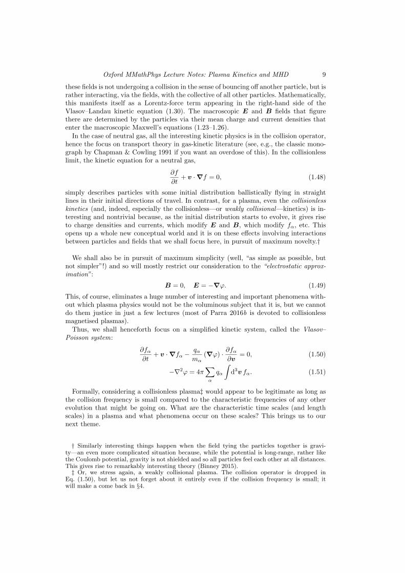
these fields is not undergoing a collision in the sense of bouncing off another particle, but israther interacting, via the fields, with the collective of all other particles. Mathematically,this manifests itself as a Lorentz-force term appearing in the right-hand side of theVlasov–Landau kinetic equation (1.30). The macroscopic E and B fields that figurethere are determined by the particles via their mean charge and current densities thatenter the macroscopic Maxwell’s equations (1.23–1.26).
In the case of neutral gas, all the interesting kinetic physics is in the collision operator,hence the focus on transport theory in gas-kinetic literature (see, e.g., the classic mono-graph by Chapman & Cowling 1991 if you want an overdose of this). In the collisionlesslimit, the kinetic equation for a neutral gas,
∂f
∂t+ v ·∇f = 0, (1.48)
simply describes particles with some initial distribution ballistically flying in straightlines in their initial directions of travel. In contrast, for a plasma, even the collisionlesskinetics (and, indeed, especially the collisionless—or weakly collisional—kinetics) is in-teresting and nontrivial because, as the initial distribution starts to evolve, it gives riseto charge densities and currents, which modify E and B, which modify fα, etc. Thisopens up a whole new conceptual world and it is on these effects involving interactionsbetween particles and fields that we shall focus here, in pursuit of maximum novelty.†
We shall also be in pursuit of maximum simplicity (well, “as simple as possible, butnot simpler”!) and so will mostly restrict our consideration to the “electrostatic approx-imation”:
B = 0, E = −∇ϕ. (1.49)
This, of course, eliminates a huge number of interesting and important phenomena with-out which plasma physics would not be the voluminous subject that it is, but we cannotdo them justice in just a few lectures (most of Parra 2016b is devoted to collisionlessmagnetised plasmas).
Thus, we shall henceforth focus on a simplified kinetic system, called the Vlasov–Poisson system:
∂fα∂t
+ v ·∇fα −qαmα
(∇ϕ) · ∂fα∂v
= 0, (1.50)
−∇2ϕ = 4π∑α
qα
∫d3v fα. (1.51)
Formally, considering a collisionless plasma‡ would appear to be legitimate as long asthe collision frequency is small compared to the characteristic frequencies of any otherevolution that might be going on. What are the characteristic time scales (and lengthscales) in a plasma and what phenomena occur on these scales? This brings us to ournext theme.
† Similarly interesting things happen when the field tying the particles together is gravi-ty—an even more complicated situation because, while the potential is long-range, rather likethe Coulomb potential, gravity is not shielded and so all particles feel each other at all distances.This gives rise to remarkably interesting theory (Binney 2015).‡ Or, we stress again, a weakly collisional plasma. The collision operator is dropped in
Eq. (1.50), but let us not forget about it entirely even if the collision frequency is small; itwill make a come back in §4.

10 A. A. Schekochihin
Figure 2. A displaced population of electrons will set up a quasineutrality-restoring electricfield, leading to plasma oscillations.
2. Equilibrium and Fluctuations
2.1. Plasma Frequency
Consider a plasma in equilibrium, in a happy quasineutral state. Suppose a populationof electrons strays from this equilibrium and upsets quasineutrality a bit (Fig. 2). If theyhave shifted by distance δx, the restoring force on each electron will be
meδx = −eE = −4πe2neδx ⇒ δx = − 4πe2neme︸ ︷︷ ︸≡ ω2
pe
δx, (2.1)
so there will be oscillations at what is known as the (electron) plasma frequency :
ωpe =
√4πe2neme
. (2.2)
Thus, we expect fluctuations of electric field in a plasma with charcteristic frequenciesω ∼ ωpe (these are Langmuir waves, we will derive their dispersion relation rigorously in§3.4). These fluctuations are due to collective motions of the particles—so they are stillmacroscopic fields in the nomenclature of §1.4.
The time scale associated with ωpe is the scale of restoration of quasineutrality. Thedistance an electron can travel over this time scale before the restoring force kicks in,i.e., the distance over which quasineutrality can be violated, is (using the thermal speedvthe ∼
√T/me to estimate the electron’s velocity)
vthe
ωpe∼√
T
me
√me
e2ne=
√T
e2ne∼ λD, (2.3)
the Debye length (1.6)—not surprising, as this is, indeed, the scale on which microscopicfields are shielded and plasma is quasineutral (§1.3).
Finally, let us check that the plasma oscillations happen on collisionless time scales.The collision frequency of the electrons is
νe ∼vthe
λmfp=vthe
ωpe
ωpe
λmfp∼ λD
λmfpωpe ωpe, q.e.d., (2.4)
using Eqs. (2.3) and (1.14).

Oxford MMathPhys Lecture Notes: Plasma Kinetics and MHD 11
2.2. Slow vs. Fast
The plasma frequency ωpe is only one of the characteristic frequencies (the largest) of thefluctuations that can occur in plasmas. We will think of the scales of all these fluctuationsas short and of the associated variation in time and space as fast. They occur against thebackground of some equilibrium state,† which is either constant or varies slowly in timeand space. The slow evolution and spatial variation of the equilibrium state can be dueto some long time and length scales on which external conditions that gave rise to thisstate change or, as we will discover soon, it can be due to the average effect of a sea ofsmall fluctuations.
Formally, this is an attempt to set up a mean-field theory, separating slow (large-scale)and fast (small-scale) parts of the distribution function:
f(r,v, t) = f0(εar,v, εt) + δf(r,v, t), (2.5)
where ε is some small parameter characterising the scale separation between fast andslow variation (note that this separation need not be the same for spatial and timescales, hence εa). To avoid clutter, we are dropping the species index where this does notlead to ambiguity.
In fact, for further simplicity, we will drop the spatial dependence of the equilibriumdistribution altogether and consider homogeneous systems:
f0 = f0(v, εt), (2.6)
which also means E0 = 0 (there is no equilibrium electric field). Equivalently, we restrictall our considerations to scales much smaller that the characteristic system size. Formally,this equilibrium distribution can be defined as the average of the exact distribution overthe volume of space that we are considering and over time scales intermediate betweenthe fast and the slow ones:‡
f0(v, t) = 〈f(r,v, t)〉 ≡ 1
∆t
∫ t+∆t/2
t−∆t/2
dt′∫
d3r
Vf(r,v, t′), (2.7)
where ω−1 ∆t equilibrium time scale.
2.3. Multiscale Dynamics
We will find it convenient to work in Fourier space:
ϕ(r, t) =∑k
eik·rϕk(t), f(r,v, t) = f0(v, t) +∑k
eik·rδfk(v, t). (2.8)
Then the Poisson equation (1.51) becomes
ϕk =4π
k2
∑α
qα
∫d3v δfkα (2.9)
† Or even just an initial state that is slow to change.‡ We use angle brackets to denote this average, but it should be clear that this is not the
same thing as the average (1.11) that allowed us to separate macroscopic fields from microscopicones. The latter was over sub-Debye scales, whereas our new average is over scales that are largerthan fluctuation scales but smaller than the system scales; both fluctuations and equilibriumare macroscopic.

12 A. A. Schekochihin
and the Vlasov equation (1.50) written for k = 0 (i.e., the spatial average of the equa-tion) is
∂f0
∂t+∂δfk=0
∂t= − q
m
∑k
ϕ−kik ·∂δfk∂v
. (2.10)
Averaging also over time according to Eq. (2.7) eliminates fast variation and gives us
∂f0
∂t= − q
m
∑k
⟨ϕ∗kik ·
∂δfk∂v
⟩(2.11)
(note that ϕ−k = ϕ∗k because ϕ(r, t) must be real).
The right-hand side of Eq. (2.11) gives us the slow evolution of the equilibrium (mean)distribution due to the effect of fluctuations. In practice, the main question is often howthe equilibrium evolves and so we need a closed equation for the evolution of f0. Thisshould be achievable at least in principle because the fluctuating fields appearing inthe right-hand side of Eq. (2.11) themselves depend on f0: indeed, writing the Vlasovequation (1.50) for the k 6= 0 modes, we find the following evolution equation for thefluctuations:
∂δfk∂t
+ ik · v δfk︸ ︷︷ ︸particle
streaming(phasemixing)
=q
mϕkik ·
∂f0
∂v︸ ︷︷ ︸wave-particleinteraction
(linear)
+q
m
∑k′
ϕk′ik′ · ∂δfk−k
′
∂v.︸ ︷︷ ︸
nonlinearinteractions
(2.12)
The three terms that control the evolution of the perturbed distribution function inEq. (2.12) represent the three physical effects that we shall focus on in these Lectures. Thesecond term on the left-hand side represents free ballistic motion of particles (“stream-ing”). It will give rise to the phenomenon of phase mixing (§4) and, in its interplay withplasma waves, to Landau damping and kinetic instabilities (§3). The first term on theright-hand side contains the interaction of the electric-field perturbations (waves) withthe equilibrium particle distribution. The second term has nonlinear interactions be-tween fluctuating fields and the perturbed distribution—it is negligible when fluctuationamplitudes are small enough (which, sadly, they rarely are) and responsible for plasmaturbulence when they are not.
The programme for determining the slow evolution of the equilibrium is “simple”: solveEq. (2.12) together with Eq. (2.9), calculate the correlation function of the fluctuations,〈ϕ∗kδfk〉, as a functional of f0, and use it to close Eq. (2.11); then proceed to solve thelatter. Obviously, this is impossible to do in most cases. But it is possible to construct ahierarchy of approximations to the answer and learn quite a lot of interesting physics inthe process.
2.4. Hierarchy of Approximations
2.4.1. Linear Theory
Consider first infinitesimal perturbations of the equilibrium. All nonlinear terms canthen be ignored, Eq. (2.11) turns into f0 = const and Eq. (2.12) becomes
∂δfk∂t
+ ik · v δfk =q
mϕkik ·
∂f0
∂v, (2.13)

Oxford MMathPhys Lecture Notes: Plasma Kinetics and MHD 13
the linearised kinetic equation. Solving this together with Eq. (2.9) allows one to tofind oscillating and/or growing/decaying† modes of the plasma perturbing a particularequilibrium. The theory for doing this is very well developed and contains some of thecore ideas that give plasma physics its intellectual shape (§3).
Physically, the linear solutions will describe what happens over short term, viz., ontimes t such that
ω−1 t teq or tnl, (2.14)
where ω is the characteristic frequency of the perturbations, teq is the time over whichthe equilibrium starts getting modified by the perturbations (which depends on theiramplitude to which they can grow: see the right-hand side of Eq. (2.11); if perturbationsgrow, they can modify the equilibrium by this mechanism so as to render it stable),and tnl is the time at which perturbation amplitudes become large enough for nonlinearinteractions between individual modes to matter (second term term on the right-handside of Eq. (2.12); if perturbations grow, they can saturate by this mechanism).
2.4.2. Quasilinear Theory (QLT)
Suppose
teq tnl, (2.15)
i.e., growing perturbations start modifying the equilibrium before they saturate nonlinearly.Then the strategy is to solve Eq. (2.13) (together with Eq. (2.9)) for the perturbations,use the result to calculate their correlation function needed in the right-hand side ofEq. (2.11), then work out how the equilibrium therefore evolves and hence how largethe perturbations must grow in order for this evolution to turn the equilibrium fromone causing the instability to a stable one. This is a classic piece of theory, importantconceptually,—we will describe it in detail and do one example in §5. In reality, however,it happens relatively rarely that unstable perturbations saturate at amplitudes smallenough for the nonlinear interactions not to matter (i.e., for tnl teq).
2.4.3. Weak-Turbulence Theory
Sometimes, one is not lucky enough to get away with QLT (so tnl . teq), but is luckyenough to have perturbations saturating nonlinearly at small amplitude such that‡
tnl ω−1, (2.16)
i.e., perturbations oscillate faster than they interact (this can happen for example becausepropagating propagating wave packets do not stay together long enough to break upcompletely in one encounter). In this case, one can do perturbation theory treating thenonlinear term in Eq. (2.12) as small and expanding in the small parameter (ωtnl)
−1.Note that because the nonlinear term couples perturbations at different k’s (scales),
this theory will lead to broad (power-law) fluctuation spectra.We will not have time for this: it’s a pity as the weak (or “wave”) turbulence theory
is quite an analytical tour de force—but a lot of work to do it properly! Classic texts onthis are Kadomtsev (1965) (early but lucid) and Zakharov et al. (1992) (mathematicallydefinitive); a recent textbook is Nazarenko (2011).
† We shall see (§4) that growing/decaying linear solutions imply the equilibrium distributiongiving/receiving energy to/from the fluctuations.‡ Note that the nonlinear time scale is typically inversely proportional to the amplitude; see
Eq. (2.12).

14 A. A. Schekochihin
2.4.4. Strong-Turbulence Theory
If perturbations manage to grow to a level at which
tnl ∼ ω−1, (2.17)
we are a facing strong turbulence. This is actually what mostly happens. Theory ofsuch regimes tends to be of phenomenological/scaling kind, usually in the spirit of theclassic Kolmogorov (1941) theory of hydrodynamic turbulence. Here is an example, notnecessarily the best or most relevant, just mine: Schekochihin et al. (2015). No one reallyknows how to do much beyond this sort of approach—and not for lack of trying (a veryrecent but historically aware review is Krommes 2015).
3. Linear Theory: Plasma Waves, Landau Damping and KineticInstablities
Enough idle chatter, let us calculate! In this section, we are concerned with the lin-earised Vlasov–Poisson system, Eqs. (2.13) and (2.9):
∂δfkα∂t
+ ik · v δfkα =qαmα
ϕkik ·∂f0α
∂v, (3.1)
ϕk =4π
k2
∑α
qα
∫d3v δfkα. (3.2)
For compactness of notation, we will drop both the species index α and the wave numberk in the subscripts, unless they are necessary for understanding.
We will discover that that electrostatic perturbations in a plasma described by Eqs. (3.1)and (3.2) oscillate, can pass their energy to particles (damp) or even grow, sucking energyfrom the particles. We will also discover that it is useful to know some complex analysis.
3.1. Initial-Value Problem
We follow Landau’s original paper (Landau 1946) in considering an initial-value problem—because, as we will see, perturbations can be damped or grow, so it is not appropriateto think of them over t ∈ [−∞,+∞] (and—NB!!!—the damped perturbations are notpure eignenmodes; see §4.3). So we look for δf(v, t) satisfying Eq. (3.1) with the initialcondition
δf(v, t = 0) = g(v). (3.3)
It is, therefore, appropriate to use Laplace transform to solve Eq. (3.1):
δf(p) =
∫ ∞0
dt e−ptδf(t) . (3.4)
It is a mathematical certainty that if there exists a real number σ > 0 such that
|δf(t)| < eσt as t→∞, (3.5)
then the integral (3.4) exists (i.e., is finite) for all values of p such that Re p > σ. Theinverse Laplace transform, giving us back our distribution function as a function of time,is then
δf(t) =1
2πi
∫ i∞+σ
−i∞+σ
dp eptδf(p), (3.6)
where the integral is along a straight line in the complex plane parallel to the imaginaryaxis and intersecting the real axis at Re p = σ (Fig. 3).

Oxford MMathPhys Lecture Notes: Plasma Kinetics and MHD 15
Figure 3. Layout of the complex-p plane: δf(p) is analytic for Re p > σ. At Re, p < σ, δf(p)may have singularities (poles).
Since we expect to be able to recover our desired time-dependent function δf(v, t) fromits Laplace transform, it is worth knowing the latter. To find it, Laplace-transform bothsides of Eq. (3.1):
l.h.s. =
∫ ∞0
dt e−pt∂δf
∂t=[e−ptδf
]∞0
+ p
∫ ∞0
dt e−ptδf = −g + p δf ,
r.h.s. = −k · v δf +q
mϕ ik · ∂f0
∂v. (3.7)
Equating these two expressions, we find the solution:
δf(p) =1
p+ ik · v
[iq
mϕ(p)k · ∂f0
∂v+ g
]. (3.8)
The Laplace transform of the potential, ϕ(p), itself depends on δf via Eq. (3.2):
ϕ(p) =
∫ ∞0
dt e−pt ϕ(t) =4π
k2
∑α
qα
∫d3v δfα(p)
=4π
k2
∑α
qα
∫d3v
1
p+ ik · v
[iqαmα
ϕ(p)k · ∂f0α
∂v+ gα
]. (3.9)
This is an algebraic equation for ϕ(p). Collecting terms, we get[1−
∑α
4πq2α
k2mαi
∫d3v
1
p+ ik · vk · ∂f0α
∂v
]︸ ︷︷ ︸
≡ ε(p,k)
ϕ(p) =4π
k2
∑α
qα
∫d3v
gαp+ ik · v
. (3.10)
The prefactor in the left-hand side, which we denote ε(p,k), is called the dielectric func-tion, because it encodes all the self-consistent charge-density perturbations that plasmasets up in response to an electric field. This is going to be an important function, so let
16 A. A. Schekochihin
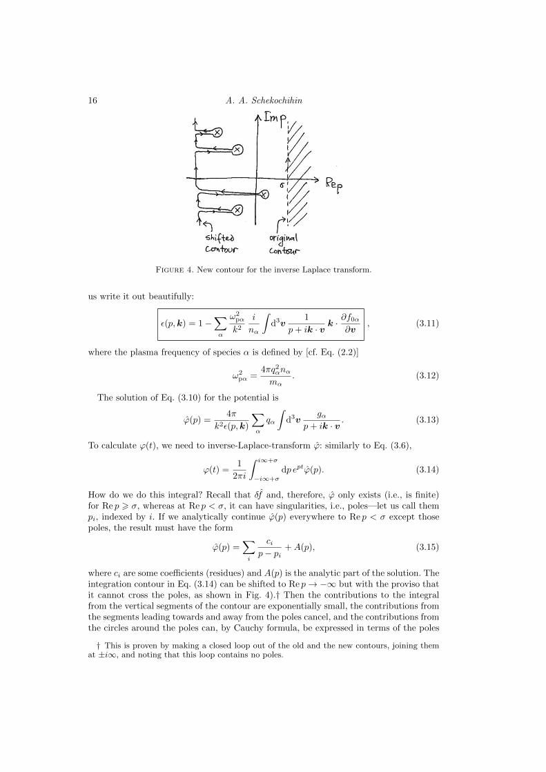
Figure 4. New contour for the inverse Laplace transform.
us write it out beautifully:
ε(p,k) = 1−∑α
ω2pα
k2
i
nα
∫d3v
1
p+ ik · vk · ∂f0α
∂v, (3.11)
where the plasma frequency of species α is defined by [cf. Eq. (2.2)]
ω2pα =
4πq2αnαmα
. (3.12)
The solution of Eq. (3.10) for the potential is
ϕ(p) =4π
k2ε(p,k)
∑α
qα
∫d3v
gαp+ ik · v
. (3.13)
To calculate ϕ(t), we need to inverse-Laplace-transform ϕ: similarly to Eq. (3.6),
ϕ(t) =1
2πi
∫ i∞+σ
−i∞+σ
dp eptϕ(p). (3.14)
How do we do this integral? Recall that δf and, therefore, ϕ only exists (i.e., is finite)for Re p > σ, whereas at Re p < σ, it can have singularities, i.e., poles—let us call thempi, indexed by i. If we analytically continue ϕ(p) everywhere to Re p < σ except thosepoles, the result must have the form
ϕ(p) =∑i
cip− pi
+A(p), (3.15)
where ci are some coefficients (residues) and A(p) is the analytic part of the solution. Theintegration contour in Eq. (3.14) can be shifted to Re p→ −∞ but with the proviso thatit cannot cross the poles, as shown in Fig. 4).† Then the contributions to the integralfrom the vertical segments of the contour are exponentially small, the contributions fromthe segments leading towards and away from the poles cancel, and the contributions fromthe circles around the poles can, by Cauchy formula, be expressed in terms of the poles
† This is proven by making a closed loop out of the old and the new contours, joining themat ±i∞, and noting that this loop contains no poles.
Oxford MMathPhys Lecture Notes: Plasma Kinetics and MHD 17
and residues:
ϕ(t) =∑i
ciepit . (3.16)
Thus, initial perturbations of the potential will evolve ∝ epit, where pi are poles of ϕ(p).In general, pi = −iωi + γi, where ωi is a real frequency (giving wave-like behaviourof perturbations), γi < 0 represents damping and γi > 0 growth of the perturbations(instability).
Going back to Eq. (3.13), we realise that the poles of ϕ(p) are zeros of the dielectricfunction:
ε(pi,k) = 0 ⇒ pi = pi(k) = −iωi(k) + γi(k). (3.17)
To find the wave frequencies ωi and the damping/growth rates γi, we must solve thisequation, which is called the plasma dispersion relation.
We are not particularly interested in what ci’s are, but they can be computed from the initialconditions, also via Eq. (3.13). The reason we are not particularly interested is that if we set upan initial perturbation with a given k and then wait long enough, only the fastest-growing or,failing growth, the slowest-damped mode will survive, with all others having exponentiall smallamplitudes. Thus, a typical outcome of the linear theory is a mode oscillating at some frequencyand growing or decaying at some rate. Since this is a linear solution, the prefactor in front ofthe exponential can be scaled arbitrarily and so does not matter.
3.2. Calculating the Dielectric Function: the “Landau Prescription”
In order to be able to solve ε(p,k) = 0, we must learn how to calculate ε(p,k) for anygiven p and k. Before I wrote Eq. (3.15), I said that ϕ, given by Eq. (3.13), had to beanalytically continued to the entire complex plane from the area where its analyticitywas guaranteed (Re p > σ), but I did not explain how this was to be done. In order to doit, we must learn how to calculate the velocity integral in Eq. (3.11)—if we want ε(p,k)and, therefore, its poles pi—and also how to calculate the similar integral in Eq. (3.13)containing gα if we also want the coefficients ci in Eq. (3.16).
First of all, let us turn these integrals into a 1D form. Given k, we can always choosethe z axis to be along k.† Then∫
d3v1
p+ ik · vk · ∂f0
∂v=
∫dvz
1
p+ ikvzk
∂
∂vz
∫dvx
∫dvy f0(vx, vy, vz)︸ ︷︷ ︸≡ F (vz)
= −i∫ +∞
−∞dvz
F ′(vz)
vz − ip/k. (3.18)
Assuming, reasonably, that F ′(vz) is a nice (analytic) function everywhere, the integrandin Eq. (3.18) has one pole, vz = ip/k. When Re p > σ > 0, this pole is harmless because,in the complex plane associated with the vz variable, it lies above the integration contour,which is along the real axis, vz ∈ (−∞,+∞). We can think of analytic continuation ofthe above integral to Re p < σ as moving the pole vz = ip/k down, towards and belowthe real axis. As long as Re p > 0, this can be done with impunity, in the sense thatthe pole stays above the integration contour, and so the natural analytic continuation issimply the same integral (3.18), still along the real axis. However, if the pole moves sofar down that Re p = 0 or Re p < 0, we must deform the contour of integration in such
† NB: This means that in what follows, k > 0 by definition.

18 A. A. Schekochihin
(a) Re p > 0 (b) Re p = 0 (c) Re p < 0
Figure 5. The Landau prescription for the contour of integration in Eq. (3.18).
Figure 6. Proof of Landau’s prescription [Eq. (3.19)].
a way as to keep the pole always above it, as shown in Fig. 5. This is called the Landauprescription and the contour thus deformed is called the Landau contour, CL.
Let us prove that this is indeed an analytic continuation, i.e., that the integral (3.18), adjustedto be along CL, is analytic for all values of p. Let us cut the Landau contour at vz = ±R andclose it in the upper half-plane with a semicircle CR of radius R such that R > σ/k (Fig. 6).Then, with integration running along the truncated CL and counterclockwise along CR, we get,by Cauchy formula,∫
CL
dvzF ′(vz)
vz − ip/k+
∫CR
dvzF ′(vz)
vz − ip/k= 2πi F ′
(ip
k
). (3.19)
Since analyticity is guaranteed for Re p > σ, the integral along CR is analytic. The right-handside is also analytic, by assumption. Therefore, the integral along CL is analytic—this is theintegral along the Landau contour if we take R→∞.
With the Landau prescription, our integral is calculated as follows:
∫CL
dvzF ′(vz)
vz − ip/k=
∫ +∞
−∞dvz
F ′(vz)
vz − ip/kif Re p > 0,
P∫ +∞
−∞dvz
F ′(vz)
vz − ip/k+ iπF ′
(ip
k
)if Re p = 0,
∫ +∞
−∞dvz
F ′(vz)
vz − ip/k+ i2πF ′
(ip
k
)if Re p < 0,
(3.20)
where the integrals are again over the real axis and the imaginary bits come from the

Oxford MMathPhys Lecture Notes: Plasma Kinetics and MHD 19
contour making a half (when Re p = 0) or a full (when Re p < 0) circle around the pole.In the case of Re p = 0, or ip = ω, the integral along the real axis is formally divergentand so we take its principal value, defined as
P∫ +∞
−∞dvz
F ′(vz)
vz − ω/k= limε→0
[∫ ω/k−ε
−∞+
∫ +∞
ω/k+ε
]dvz
F ′(vz)
vz − ω/k. (3.21)
The difference between Eq. (3.21) and the usual Lebesgue definition of an integral is that thelatter would be∫ +∞
−∞dvz
F ′(vz)
vz − ω/k=
[limε1→0
∫ ω/k−ε1
−∞+ limε2→0
∫ +∞
ω/k+ε2
]dvz
F ′(vz)
vz − ω/k, (3.22)
and this, with, in general, ε1 6= ε2, diverges logarithmically, whereas in Eq. (3.21), the divergencesneatly cancel.
The Re p = 0 case in Eq. (3.20),∫CL
dvzF ′(vz)
vz − ω/k= P
∫ +∞
−∞dvz
F ′(vz)
vz − ω/k+ iπF ′
(ωk
), (3.23)
which tends to be of most use in analytical theory, is a particular instance of Plemelj’s formula:for a real ζ and a well-behaved function f (no poles on or near the real axis),
limε→+0
∫ +∞
−∞dx
f(x)
x− ζ ∓ iε = P∫ +∞
−∞dx
f(x)
x− ζ ± iπf(ζ), (3.24)
also sometimes written as
limε→+0
1
x− ζ ∓ iε = P 1
x− ζ ± iπδ(ζ), (3.25)
Finally, armed with Landau’s prescription, we are ready to calculate. Eq. (3.11) becomes
ε(p,k) = 1−∑α
ω2pα
k2
1
nα
∫CL
dvzF ′α(vz)
vz − ip/k(3.26)
and, analogously, Eq. (3.13) becomes
ϕ(p) = − 4πi
k3ε(p,k)
∑α
qα
∫CL
dvzGα(vz)
vz − ip/k, (3.27)
where Gα(vz) =∫
dvx∫
dvy gα(vx, vy, vz).
3.3. Solving the Dispersion Relation: Slow-Damping/Growth Limit
A particularly analytically solvable and physically interesting case is one in which, forp = −iω + γ, γ ω (or, if ω = 0, γ kvthα), i.e., the case of slow damping or growth.In this limit, the dispersion relation is
ε(p,k) ≈ ε(−iω,k) + iγ∂
∂ωε(−iω,k) = 0. (3.28)
Setting the imaginary part of Eq. (3.28) to zero gives us the growth/damping rate interms of the real frequency:
γ = −Im ε(−iω,k)
[∂
∂ωRe ε(−iω,k)
]−1
. (3.29)

20 A. A. Schekochihin
Setting the real part of Eq. (3.28) to zero gives the equation for the real frequency:
Re ε(−iω,k) = 0 . (3.30)
Thus, we now only need ε(p,k) with p = −iω. Using Eq. (3.23), we get
Re ε = 1−∑α
ω2pα
k2
1
nαP∫
dvzF ′α(vz)
vz − ω/k, (3.31)
Im ε = −∑α
ω2pα
k2
π
nαF ′α
(ωk
). (3.32)
Let us now consider a two-species plasma, consisting of electrons and a single speciesof ions. There will be two interesting limits:
• “High-frequency” electron waves: ω kvthe, where vthe =√
2Te/me is the “thermalspeed” of the electrons†; this limit will give us Langmuir waves (§3.4), slowly damped orgrowing (§3.5).• “Low-frequency” ion waves: a particularly tractable limit will be that of “hot” elec-
trons and “cold” ions, viz., kvthe ω kvthi, where vthi =√
2Ti/mi is the “thermalspeed” of the ions; this limit will give us the sound (“ion-acoustic waves”; §3.7), whichalso can be damped or growing (§3.8).
3.4. Langmuir Waves
Consider the limit
ω
k vthe, (3.33)
i.e., the phase velocity of the waves is much greater than the typical velocity of a particalfrom the “thermal bulk” of the distribution. This means that in Eq. (3.31), we can expandin vz ∼ vthe small compared to ω/k (higher values of vz are cut off by the equilibriumdistribution function). Note that ω kvthe also implies ω kvthi because
vthi
vthe=
√TiTe
me
mi 1 (3.34)
† This is a standard well-defined quantity for a Maxwellian equilibrium distributionFe(vz) = (ne/
√π vthe) exp(−v2z/v2the), but if we wish to consider a non-Maxwellian Fe, let vthe
be a typical speed characterising the width of the equilibrium distribution, defined by, e.g.,Eq. (3.36).

Oxford MMathPhys Lecture Notes: Plasma Kinetics and MHD 21
as long as Ti/Te is not huge.‡ Thus, Eq. (3.31) becomes
Re ε = 1 +∑α
ω2pα
k2
1
nα
k
ωP∫
dvz F′α(vz)
[1 +
kvzω
+
(kvzω
)2
+
(kvzω
)3
+ . . .
]
= 1 +∑α
ω2pα
kω
[1
nα
∫dvz F
′α(vz)︸ ︷︷ ︸
= 0
− kω
1
nα
∫dvz Fα(vz)︸ ︷︷ ︸= 1
− 2k2
ω2
1
nα
∫dvz vzFα(vz)︸ ︷︷ ︸
= 0
−3k3
ω3
1
nα
∫dvz v
2zFα(vz)︸ ︷︷ ︸
= v2thα/2
+ . . .
]
= 1−∑α
ω2pα
ω2
[1 +
3
2
k2v2thα
ω2+ . . .
], (3.35)
where we have integrated by parts everywhere, assumed that there are no mean flows,〈vz〉 = 0, and, in the last term, used
〈v2z〉 =
v2thα
2, (3.36)
which is indeed the case for a Maxwellian Fα or, if Fα is not a Maxwellian, can be viewedas the definition of vthα.
The ion contribution to Eq. (3.35) is small because
ω2pi
ω2pe
=Zme
mi 1. (3.37)
Therefore, to lowest order, the dispersion relation Re ε = 0 becomes
1−ω2
pe
ω2= 0 ⇒ ω2 = ω2
pe =4πe2neme
, (3.38)
the Tonks & Langmuir (1929) dispersion relation for what is known as Langmuir, orplasma, oscillations. This is the formal derivation of the result that we already had, onphysical grounds, in §2.1.
We can do a little better if we retain the (small) k-dependent term in Eq. (3.35):
Re ε ≈ 1−ω2
pe
ω2
(1 +
3
2
k2v2the
ω2︸ ︷︷ ︸use
ω2 ≈ ω2pe
)= 0 ⇒ ω2 ≈ ω2
pe(1 + 3k2λ2De) , (3.39)
where λDe = vthe/√
2ωpe =√Te/4πe2ne is the “electron Debye length” [cf. Eq. (1.6)].
Eq. (3.39) is the Bohm & Gross (1949) dispersion relation, describing an upgrade ofthe Langmuir oscillations to dispersive Langmuir waves, which have a non-zero groupvelocity.
Note that all this is only valid for ω kvthe, which we now see is equivalent to
kλDe 1. (3.40)
‡ For hydrogen plasma,√mi/me ≈ 42, more or less, the answer to the Ultimate Question of
Life, Universe and Everything (Adams 1979).
22 A. A. Schekochihin
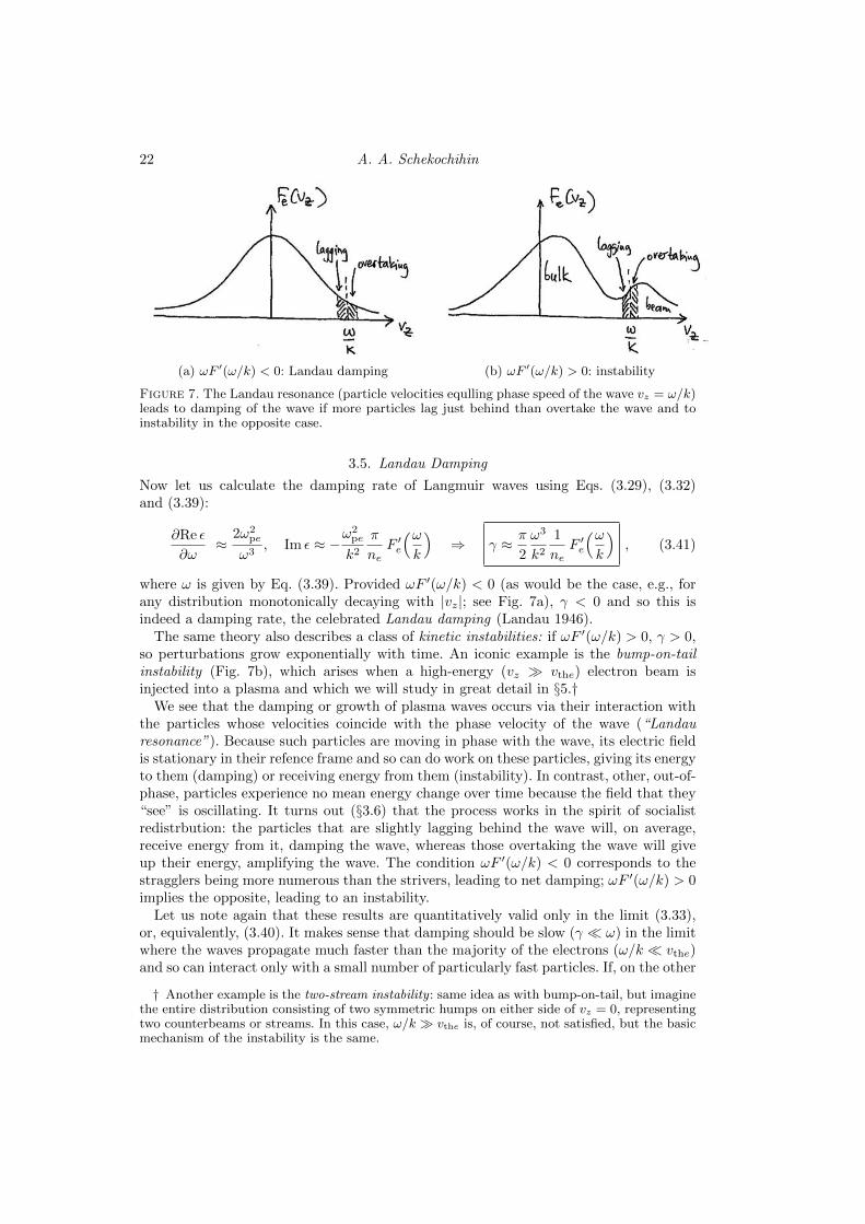
(a) ωF ′(ω/k) < 0: Landau damping (b) ωF ′(ω/k) > 0: instability
Figure 7. The Landau resonance (particle velocities equlling phase speed of the wave vz = ω/k)leads to damping of the wave if more particles lag just behind than overtake the wave and toinstability in the opposite case.
3.5. Landau Damping
Now let us calculate the damping rate of Langmuir waves using Eqs. (3.29), (3.32)and (3.39):
∂Re ε
∂ω≈
2ω2pe
ω3, Im ε ≈ −
ω2pe
k2
π
neF ′e
(ωk
)⇒ γ ≈ π
2
ω3
k2
1
neF ′e
(ωk
), (3.41)
where ω is given by Eq. (3.39). Provided ωF ′(ω/k) < 0 (as would be the case, e.g., forany distribution monotonically decaying with |vz|; see Fig. 7a), γ < 0 and so this isindeed a damping rate, the celebrated Landau damping (Landau 1946).
The same theory also describes a class of kinetic instabilities: if ωF ′(ω/k) > 0, γ > 0,so perturbations grow exponentially with time. An iconic example is the bump-on-tailinstability (Fig. 7b), which arises when a high-energy (vz vthe) electron beam isinjected into a plasma and which we will study in great detail in §5.†
We see that the damping or growth of plasma waves occurs via their interaction withthe particles whose velocities coincide with the phase velocity of the wave (“Landauresonance”). Because such particles are moving in phase with the wave, its electric fieldis stationary in their refence frame and so can do work on these particles, giving its energyto them (damping) or receiving energy from them (instability). In contrast, other, out-of-phase, particles experience no mean energy change over time because the field that they“see” is oscillating. It turns out (§3.6) that the process works in the spirit of socialistredistrbution: the particles that are slightly lagging behind the wave will, on average,receive energy from it, damping the wave, whereas those overtaking the wave will giveup their energy, amplifying the wave. The condition ωF ′(ω/k) < 0 corresponds to thestragglers being more numerous than the strivers, leading to net damping; ωF ′(ω/k) > 0implies the opposite, leading to an instability.
Let us note again that these results are quantitatively valid only in the limit (3.33),or, equivalently, (3.40). It makes sense that damping should be slow (γ ω) in the limitwhere the waves propagate much faster than the majority of the electrons (ω/k vthe)and so can interact only with a small number of particularly fast particles. If, on the other
† Another example is the two-stream instability : same idea as with bump-on-tail, but imaginethe entire distribution consisting of two symmetric humps on either side of vz = 0, representingtwo counterbeams or streams. In this case, ω/k vthe is, of course, not satisfied, but the basicmechanism of the instability is the same.
Oxford MMathPhys Lecture Notes: Plasma Kinetics and MHD 23
hand, ω/k ∼ vthe, the waves interact with the majority population and the dampingshould be strong: a priori, we might expect γ ∼ kvthe.
3.6. Physical Picture of Landau Damping
The following simple argument (Lifshitz & Pitaevskii 1981) illustrates the physical mechanismof Landau damping.
Consider an electron moving along the z axis, subject to a wave-like electric field:
dz
dt= vz, (3.42)
dvzdt
= − e
meE(z, t) = − e
meE0 cos(ωt− kz)eεt. (3.43)
We have given the electric field a slow time dependence, E ∝ eεt, where we will later takeε → +0—this describes the field switching on infinitely slowly from t = −∞. We assume thatthe amplitude E0 of the electric field is so small that it changes the electron’s trajectory only alittle over several wave periods. Then we can solve the equations of motion perturbatively.
The lowest-order (E0 = 0) solution is
vz(t) = v0 = const, z(t) = v0t. (3.44)
In the next order, we let
vz(t) = v0 + δvz(t), z(t) = v0t+ δz(t). (3.45)
Eq. (3.43) becomes
dδvzdt
= − e
meE(z(t), t) ≈ − e
meE(v0t, t) = −eE0
meRe e[i(ω−kv0)+ε]t. (3.46)
Integrating this gives
δvz(t) = −eE0
me
∫ t
0
dt′Re e[i(ω−kv0)+ε]t′
= −eE0
meRe
e[i(ω−kv0)+ε]t − 1
i(ω − kv0) + ε
= −eE0
me
εeεt cos[(ω − kv0)t]− ε+ (ω − kv0)eεt sin[(ω − kv0)t]
(ω − kv0)2 + ε2. (3.47)
Integrating again,
δz(t) =
∫ t
0
dt′ δvz(t′)
= −eE0
me
∫ t
0
dt′Ree[i(ω−kv0)+ε]t
′− 1
i(ω − kv0) + ε
= −eE0
me
Re
e[i(ω−kv0)+ε]t − 1
[i(ω − kv0) + ε]2− εt
(ω − kv0)2 + ε2
= −eE0
me
[ε2 − (ω − kv0)2
] eεt cos[(ω − kv0)t]− 1
+ 2ε(ω − kv0)eεt sin[(ω − kv0)t]
[(ω − kv0)2 + ε2]2
− εt
(ω − kv0)2 + ε2
. (3.48)
The work done by the field on the electron per unit time, averaged over time, is the power gained

24 A. A. Schekochihin
Figure 8. The function χ(v0) defined in Eq. (3.49).
by the electron:
δP (v0) = −e 〈E(z(t), t)vz(t)〉
≈ −e⟨[E(v0t, t) + δz(t)
∂E
∂z(v0t, t)
][v0 + δvz(t)]
⟩= −eE0e
εt
⟨v0 cos[(ω − kv0)t]︸ ︷︷ ︸
vanishesunder
averaging
+ δvz(t) cos[(ω − kv0)t]︸ ︷︷ ︸only cos term
fromEq. (3.47)survives
averaging
+ v0δz(t)k sin[(ω − kv0)t]︸ ︷︷ ︸only sin term
fromEq. (3.48)survives
averaging
⟩
=e2E2
0
2mee2εt
ε
(ω − kv0)2 + ε2+
2kv0ε(ω − kv0)
[(ω − kv0)2 + ε2]2
=e2E2
0
2mee2εt
d
dv0
εv0(ω − kv0)2 + ε2︸ ︷︷ ︸≡ χ(v0)
. (3.49)
We see that (Fig. 8)—if the electron is lagging behind the wave, v0 . ω/k, then χ′(v0) > 0 ⇒ δP (v0) > 0, soenergy goes from the field to the electron (the wave is damped);—if the electron is overtaking the wave, v0 & ω/k, then χ′(v0) < 0 ⇒ δP (v0) < 0, so energygoes from the electron to the field (the wave is amplified).
Now remember that we have a whole distribution of these electrons, F (vz). So the total powerper unit volume going into (or out of) them is
P =
∫dvz F (vz)δP (vz) =
e2E20e
2εt
2me
∫dvz F (vz)χ
′(vz)
= −e2E2
0e2εt
2me
∫dvz F
′(vz)χ(vz). (3.50)
Noticing that, by Plemelj’s formula (3.25), in the limit ε→ +0,
χ(vz) =εvz
(ω − kvz)2 + ε2= − ivz
2
(1
kvz − ω − iε− 1
kvz − ω + iε
)→ π
ω
k2δ(vz −
ω
k
), (3.51)
we conclude
P = − e2E20
2mek2πωF ′
(ωk
). (3.52)
As in §3.5, we find damping if ωF ′(ω/k) < 0 and instability if ωF ′(ω/k) > 0.Thus, around the wave-particle resonance vz = ω/k, the particles just lagging behind the
wave receive energy from the wave and those just overtaking it give up energy to it. Therefore,qualitatively, damping occurs if the former particles are more numerous than the latter. We seethat Landau’s mathematics in §§3.1–3.5 led us to a result that makes physical sense.
Oxford MMathPhys Lecture Notes: Plasma Kinetics and MHD 25
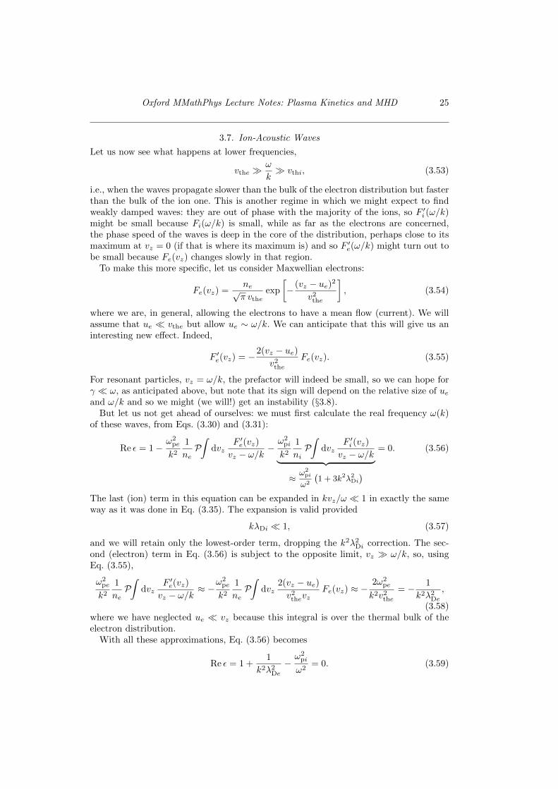
3.7. Ion-Acoustic Waves
Let us now see what happens at lower frequencies,
vthe ω
k vthi, (3.53)
i.e., when the waves propagate slower than the bulk of the electron distribution but fasterthan the bulk of the ion one. This is another regime in which we might expect to findweakly damped waves: they are out of phase with the majority of the ions, so F ′i (ω/k)might be small because Fi(ω/k) is small, while as far as the electrons are concerned,the phase speed of the waves is deep in the core of the distribution, perhaps close to itsmaximum at vz = 0 (if that is where its maximum is) and so F ′e(ω/k) might turn out tobe small because Fe(vz) changes slowly in that region.
To make this more specific, let us consider Maxwellian electrons:
Fe(vz) =ne√π vthe
exp
[− (vz − ue)2
v2the
], (3.54)
where we are, in general, allowing the electrons to have a mean flow (current). We willassume that ue vthe but allow ue ∼ ω/k. We can anticipate that this will give us aninteresting new effect. Indeed,
F ′e(vz) = −2(vz − ue)v2
the
Fe(vz). (3.55)
For resonant particles, vz = ω/k, the prefactor will indeed be small, so we can hope forγ ω, as anticipated above, but note that its sign will depend on the relative size of ueand ω/k and so we might (we will!) get an instability (§3.8).
But let us not get ahead of ourselves: we must first calculate the real frequency ω(k)of these waves, from Eqs. (3.30) and (3.31):
Re ε = 1−ω2
pe
k2
1
neP∫
dvzF ′e(vz)
vz − ω/k−ω2
pi
k2
1
niP∫
dvzF ′i (vz)
vz − ω/k︸ ︷︷ ︸≈ω2pi
ω2
(1 + 3k2λ2
Di
)= 0. (3.56)
The last (ion) term in this equation can be expanded in kvz/ω 1 in exactly the sameway as it was done in Eq. (3.35). The expansion is valid provided
kλDi 1, (3.57)
and we will retain only the lowest-order term, dropping the k2λ2Di correction. The sec-
ond (electron) term in Eq. (3.56) is subject to the opposite limit, vz ω/k, so, usingEq. (3.55),
ω2pe
k2
1
neP∫
dvzF ′e(vz)
vz − ω/k≈ −
ω2pe
k2
1
neP∫
dvz2(vz − ue)v2
thevzFe(vz) ≈ −
2ω2pe
k2v2the
= − 1
k2λ2De
,
(3.58)where we have neglected ue vz because this integral is over the thermal bulk of theelectron distribution.
With all these approximations, Eq. (3.56) becomes
Re ε = 1 +1
k2λ2De
−ω2
pi
ω2= 0. (3.59)

26 A. A. Schekochihin
The dispersion relation is then
ω2 =ω2
pi
1 + 1/k2λ2De
=k2c2s
1 + k2λ2De
, (3.60)
where
cs = ωpiλDe =
√ZTemi
(3.61)
is the sound speed, called that because, assuming further kλDe 1, Eq. (3.60) describesa wave that is very obviously a sound, or ion-acoustic, wave:
ω = ±kcs . (3.62)
The phase speed of this wave is the sound speed, ω/k = cs.We can now check under what circumstances the condition (3.53) is indeed satisfied:
csvthe
=
√Zme
mi 1,
csvthi
=
√ZTeTi 1, (3.63)
with the latter condition requiring that the ions should be colder than the electrons.
3.8. Damping of Ion-Acoustic Waves and Ion-Acoustic Instability
Are ion acoustic waves damped? Can they grow? We have a standard protocol for answer-ing this question: calculate Re ε and Im ε and substitute into Eq. (3.29). Using Eqs. (3.59)and (3.32), we find
∂Re ε
∂ω=
2ω2pi
ω3, Im ε = −
ω2pe
k2
π
neF ′e
(ωk
)−ω2
pi
k2
π
niF ′i
(ωk
). (3.64)
The two terms in Im ε represent the interaction between the waves and, respectively,electrons and ions. The ion term is small both on account of ωpi ωpe and, assumingMaxwellian ions, of the exponential smallness of Fi(ω/k) ∝ exp[−(ω/kvthi)
2]. We arethen left with
γ = − Im ε
∂(Re ε)/∂ω= −√π
ω3
k2v3the
mi
Zme
(ωk− ue
), (3.65)
where we have used Eq. (3.55). In the long-wavelength limit, kλDe 1, we have ω =±kcs, and so, for the “+” mode,
γ = −√πZme
8mik (cs − ue) . (3.66)
If the electron flow is subsonic, ue < cs, this describes the Landau damping of ion acousticwaves on hot electrons. If, on the other hand, the electron flow is supersonic, the signof γ reverses† and we discover the ion-acoustic instability: excitation of ion acousticwaves by fast electron current.‡ The instability belongs to the same general class as,e.g., the bump-on-tail instability (§3.5) in that it involves waves sucking energy fromparticles, but the new conceptual feature here is that such energy conversion can resultfrom a collaboration between different particle species (electrons supplying the energy,ions carrying the wave).
There is a host of related instabilities involving various combinations of electron and
† Recall that k > 0 by the choice of the z axis.‡ As far as I can tell, the original reference on this instability mechanism is Buneman (1958).

Oxford MMathPhys Lecture Notes: Plasma Kinetics and MHD 27
Figure 9. Electrostatic (longitudinal) plasma waves.
ion beams, currents, streams and counterstreams—an excellent treatment of them canbe found in Davidson (1983).
Exercise 3.1. Find the ion contribution to the damping of ion-acoustic waves. Under whatconditions does it become comparable to, or larger than, the electron contribution?
3.9. Ion Langmuir Waves
Note that since
λDe
λDi=vtheωpi
vthiωpe=
√ZTeTi
, (3.67)
the condition (3.57) need not entail kλDe 1 in the limit of cold ions, Eq. (3.63)—inthis case the size of the Debye sphere (1.6) is set by the ions, rather than the electrons,and so we can have perfectly macroscopic (in the language of §1.4) perturbations onscales both larger and smaller than λDe. At larger scales, we have found sound waves(3.62). At smaller scales, kλDe 1, the dispersion relation (3.60) gives us ion Langmuiroscillations:
ω2 = ω2pi =
4πZ2e2nimi
, (3.68)
which are analogous to the electron Langmuir oscillations (3.38) and, like them, turn intodispersive ion Langmuir waves if the small k2λ2
Di correction in Eq. (3.56) is retained,leading to the Bohm–Gross dispersion relation (3.39), but with ion quantities this time.
Exercise 3.2. Derive the dispersion relation for ion Langmuir waves. Investigate their damp-ing/instability.
28 A. A. Schekochihin
3.10. Summary of Electrostatic (Longitudinal) Plasma Waves
We have achieved what turns out to be a basically complete characterisation of electro-static (also known as “longitudinal”, in the sense that k ‖ E) waves in an unmagnetisedplasma. These are summarised in Fig. 9. In the limit of short wavelengths, kλDe 1 andkλDi 1, the electron and ion branches, respectively, becomes dispersive, their dampingrates increase and eventually stop being small. This corresponds to waves having phasespeeds that are comparable to the speeds of the particles in the thermal bulk of theirdistributions, so a great number of particles are available to have Landau resonance withthe waves and absorb their energy—the damping becomes strong.
Note that if the cold-ion condition Ti Te is not satisfied, the sound speed is coma-parable to the ion thermal speed cs ∼ vthi, and so the ion-acoustic waves are stronglydamped at all wave numbers—it is well-nigh impossible to propagate sound through acollisionless hot plasma!
3.11. Plasma Dispersion Function: Putting Linear Theory on Industrial Basis
By the end of this section, we have entered the realm of practical calculation—it is now easy toimagine an industry of solving the plasma dispersion relation
ε(p,k) = 1−∑α
ω2pα
k21
nα
∫CL
dvzF ′α(vz)
vz − ip/k= 0 (3.69)
and similar dispersion relations arising from, e.g., considering electromagnetic perturbations,magnetised plasmas, different equilibria Fα, etc.
It is obviously an extremely important special case to consider a Maxwellian equilibriumbecause that is, after all, the direction in which plasma is pushed by collisions on long timescales:
f0α(v) =nα
(πv2thα)3/2e−v
2/v2thα ⇒ Fα(vz) =nα√πvthα
e−v2z/v
2thα . (3.70)
For this case, we would like to introduce a new “special function” that would incorporate theLandau prescription for calculating the velocity integral in Eq. (3.69) and that we could in somesense “tabulate” once and for all.†
Taking Fα to be a Maxwellian and letting u = vz/vthα and ζα = ip/kvthα, we can rewrite thevelocity integral in Eq. (3.69) as follows
1
nα
∫CL
dvzF ′α(vz)
vz − ip/k= − 2√
π v2thα
∫CL
duu e−u
2
u− ζα= − 2
v2thα[1 + ζαZ(ζα)] , (3.71)
where the plasma dispersion function is defined to be
Z(ζ) =1√π
∫du
e−u2
u− ζ . (3.72)
In these terms, the plasma dispersion relation (3.69) becomes
ε = 1 +∑α
1 + ζαZ(ζα)
k2λ2Dα
= 0 . (3.73)
Note that if the Maxwellian distribution (3.70) has a mean flow, as it did, e.g., in Eq. (3.54),this amounts to a shift by some mean velocity uα and all one needs to do to adjust the aboveresults is to shift the argument of Z accordingly:
ζα → ζα −uαvthα
. (3.74)
† In the olden days, we would literally tabulate it (Fried & Conte 1961). In the 21st century,we could just teach a computer to compute it [see Eq. (3.79)] and have an app.

Oxford MMathPhys Lecture Notes: Plasma Kinetics and MHD 29
3.11.1. Some Properties of Z(ζ)
It is not hard to see that
Z′(ζ) = − 1√π
∫du e−u
2 ∂
∂u
1
u− ζ = − 2√π
∫du
u e−u2
u− ζ = −2 [1 + ζZ(ζ)] . (3.75)
Let us treat this identity as a differential equation: the integrating factor is eζ2
and so
eζ2
Z(ζ) = −2
∫ ζ
0
dt et2
+ Z(0). (3.76)
We know the boundary condition at ζ = 0 from Plemelj’s formula (3.23): for real ζ,
1√π
∫du
e−u2
u− ζ =1√πP∫ +∞
−∞du
e−u2
u− ζ︸ ︷︷ ︸= 0 for ζ = 0
becauseintegrand is
odd
+ i√π e−ζ
2
⇒ Z(0) = i√π. (3.77)
Using this in Eq. (3.76) and changing the integration variable t = −ix, we find
Z(ζ) = e−ζ2(i√π + i
∫ iζ
0
dx e−x2)
= 2i e−ζ2∫ iζ
−∞dx e−x
2
. (3.78)
This turns out to be a uniformly valid expression for Z(ζ): our function is simply a complex erf!Here is a Mathematica script for calculating it:
Z[zeta ] := I Sqrt[Pi] Exp[−zeta2](1 + I Erfi[zeta]). (3.79)
You can use this to code up Eq. (3.73) and explore, e.g., the strongly damped solutions (ζ ∼ 1,γ ∼ ω).
3.11.2. Asymptotics of Z(ζ)
If you believe in preserving the ancient art of asymptotic theory, you will find most useful(as, effectively, we did in §§3.4–3.8) various limiting forms of Z(ζ). At small argument |ζ| 1,the Taylor series is
Z(ζ) = i√π e−ζ
2
− 2ζ
(1− 2ζ2
3+
4ζ4
15− 8ζ6
105+ . . .
). (3.80)
At large argument, |ζ| 1, |Re ζ| |Im ζ|, the asymptotic series is
Z(ζ) = i√π e−ζ
2
− 1
ζ
(1 +
1
2ζ2+
3
4ζ4+
15
8ζ6+ . . .
). (3.81)
All the results (for a Maxwellian equilibrium) that I derived in §§3.4–3.9 can be readily obtainedfrom Eq. (3.73) by using the above limiting cases. It is, indeed, a general practical strategy forstudying this and similar plasma dispersion relations to look for solutions in the limits ζα → 0 orζα →∞, then check under what physical conditions the solutions thus obtained are valid (i.e.,they indeed satisfy |ζα| 1 or |ζα| 1, |Re ζ| |Im ζ|), and then fill in the non-asymptoticblanks in the same way that an experienced hunter espying antlers sticking out above theshrubbery can reconstruct, in contour outline, the rest of the hiding deer.
Exercise 3.3. Work out the Taylor series (3.80). A useful step might be to prove this interestingformula (which also turns out to be handy in other calculations; see, e.g., Q6):
dmZ
dζm=
(−1)m√π
∫CL
duHm(u) e−u
2
u− ζ , (3.82)
where Hm(u) are Hermite polynomials.

30 A. A. Schekochihin
Exercise 3.4. Work out the asymptotic series (3.81) using the Landau prescription (3.20) andexpanding the principal-value integral similarly to the way it was done in Eq. (3.35). Work outalso (or look up; e.g., Fried & Conte 1961) other asymptotic forms of Z(ζ), relaxing the condition|Re ζ| |Im ζ|.
4. Energy, Entropy, Free Energy, Heating, Irreversibility and PhaseMixing
While we are done with the “calculational” part of linear theory (calculating the ratesat which field perturbations oscillate, damp or grow), we are not yet done with the“conceptual” part: what exactly is going on, mathematically and physically? The planof addressing this question in this section is as follows.• I will show that Landau damping of perturbations of a plasma in thermal equilibrium
leads to the heating of this equilibrium—basically, that energy is conserved. This is nota surprise, but it is useful to see explicitly how this works (§4.1).• I will then ask how it is possible to have heating (an irreversible process) in a plasma
that was assumed collisionless and must conserve entropy. In other words, why, physically,is Landau damping a damping? This will lead us to consider entropy evolution in oursystem and to stumble on an important concept of free energy (§4.2).• In the above context, we will examine (§§4.3, 4.5) the Laplace-transform solution
(3.8) for the perturbed distribution function and establish the phenomenon of phasemixing—emergence of fine structure in velocity (phase) space. This will allow collisionsand, therefore, irreversiblity back in (§4.4). We will also see that the Landau-dampedsolutions are not eigenmodes (while growing solutions can be), and so conclude that itmade sense to insist on using an initial-value-problem formalism.
4.1. Energy Conservation and Heating
Let us go back to the full, nonlinear Vlasov–Poisson system, where we now restore thecollision term:
∂fα∂t
+ v ·∇fα −qαmα
(∇ϕ) · ∂fα∂v
=
(∂fα∂t
)c
, (4.1)
−∇2ϕ = 4π∑α
qα
∫d3v fα. (4.2)
Let us calculate the rate of change of the electric energy:
d
dt
∫d3r
E2
8π=
∫d3r
∇ϕ
4π· ∂(∇ϕ)
∂t︸ ︷︷ ︸by parts
= −∫
d3rϕ
4π
∂
∂t∇2ϕ︸ ︷︷ ︸
useEq. (4.2)
=∑α
qα
∫∫d3r d3v ϕ
∂fα∂t︸ ︷︷ ︸
useEq. (4.1)
=∑α
qα
∫∫d3r d3v ϕ
[−v ·∇fα︸ ︷︷ ︸by parts
+qαmα
(∇ϕ) · ∂f∂v︸ ︷︷ ︸
vanishesbecause
f(±∞) = 0
+
(∂fα∂t
)c︸ ︷︷ ︸
vanishesbecause
number ofparticles isconserved
]
=∑α
qα
∫∫d3r d3v fαv ·∇ϕ = −
∫d3rE · j, (4.3)

Oxford MMathPhys Lecture Notes: Plasma Kinetics and MHD 31
where j is the current density. So the rate of change of the electric field is minus the rateat which electric field does work on the charges, a.k.a. Joule heating—not a surprisingresult. The energy goes into accelerating particles, of course: the rate of change of theirenergy is
dU
dt=∑α
∫∫d3r d3v
mαv2
2
∂fα∂t︸ ︷︷ ︸
useEq. (4.1)
=∑α
∫∫d3r d3v
m2α
2
[−v ·∇fα︸ ︷︷ ︸vanishesbecause
fulldivergence
+qαmα
(∇ϕ) · ∂fα∂v︸ ︷︷ ︸
by parts in v
+
(∂fα∂t
)c︸ ︷︷ ︸
vanishesbecauseenergy isconserved
]
= −∑α
qα
∫∫d3r d3v fαv ·∇ϕ =
∫d3rE · j. (4.4)
Combining Eqs. (4.3) and (4.4) gives us the law of energy conservation:
d
dt
(U +
∫d3r
E2
8π
)= 0 . (4.5)
Exercise 4.1. Demonstrate energy conservation for the more general case in which magnetic-field perturbations are also allowed.
Thus, if the perturbations are damped, the energy of the particles must increase—this is usually called heating. Strictly speaking, heating refers to a slow increase in themean temperature of the thermal equilibrium. Let us make this statement quantitative.Consider a Maxwellian plasma, homogeneous in space but possibly with some slow de-pendence on time (cf. §2):
f0α =nα
(πv2thα)3/2
e−v2/v2thα = nα
(mα
2πTα
)3/2
e−mαv2/2Tα . (4.6)
In a homoegeneous system with a fixed volume, the density nα is constant in timebecause the number of particles is constant: d(V nα)/dt = 0. We allow, however, that thetemperature is Tα = Tα(t). The total kinetic energy of the particles is
U = V∑α
∫d3v
mαv2
2f0α︸ ︷︷ ︸
=3
2nαTα
+∑α
∫∫d3r d3v
mαv2
2δfα. (4.7)
Let us average this over time, as per Eq. (2.7): the perturbed part vanishes and we have
〈U〉 = V∑α
3
2nαTα. (4.8)
Averaging also Eq. (4.5) and using Eq. (4.8), we get∑α
3
2nα
dTαdt
= − d
dt
1
V
∫d3r〈E2〉8π
, (4.9)
32 A. A. Schekochihin
the heating rate of the equilibrium equals the rate of decrease of the mean energy of theperturbations.
We saw that the perturbations evolve according to Eq. (3.16). If we wait for a while,only the slowest-damped mode will matter, with all others exponentially small. Let uscall its frequency and its damping rate ωk and γk < 0, respectively, so Ek ∝ e−iωkt+γkt.If we assume that |γk| ωk, we may define the averge (2.7) in such a way that ω−1
k ∆t |γk|−1. Then Eq. (4.9) becomes∑
α
3
2nα
dTαdt
= −∑k
2γk|Ek|2
8π> 0 if γk < 0. (4.10)
The Landau damping rate of the electric-field perturbation is the heating rate of theequilibrium.†
This result, while at first glance utterly obvious, might also, on reflection, appear to beparadoxical: surely, the heating of the equilibrium implies increasing entropy—but thedamping that is leading to the heating is collisionless and, in a collisionless system, inview of the H theorem, how can the entropy change?
4.2. Entropy and Free Energy
The kinetic entropy for each species of particles is defined
Sα = −∫∫
d3r d3v fα ln fα. (4.11)
This quantity (or, indeed, the full-phase-space integral of any quantity that is a functiononly of fα) can only be changed by collisions and, furthermore, the plasma-physics versionof Boltzmann’s H theorem establishes that
d
dt
∑α
Sα = −∑α
∫∫d3r d3v
(∂fα∂t
)c
ln fα > 0, (4.12)
where equality is achieved iff all fα are Maxwellian with the same temperature Tα = T .Thus, if collisions are ignored, the total entropy stays constant and everything that
happens is, in principle, reversible. So how can there be net damping and, worse still, netheating?! Presumably, any damping solution can be turned into a growing solution byreversing all particle trajectories—so should the overall perturbation level stay constant?
As we already noted in §4.1, strictly speaking, heating is the change in the equilibriumtemperature—and, therefore, equilibrium entropy. Indeed, for each species, the equilib-rium entropy is
S0 = −∫∫
d3r d3v f0 ln f0 = −∫∫
d3r d3v f0
ln
[n(m
2π
)3/2]− 3
2lnT − mv2
2T
= V
[−n lnn
(m2π
)3/2
+3
2n lnT +
3
2n
], (4.13)
where we have used∫
d3v (mv2/2)f0 = (3/2)nT . Since n = const,
TdS0
dt= V
3
2n
dT
dt, (4.14)
so heating [see Eq. (4.9)] is indeed associated with the increase of S0.Since, according to Eq. (4.10), this can be successfully accomplished by collisionless
damping and since entropy overall can only increase due to collisions, we must search
† Obviously, the damping on a species α increases only the temperature of that species.

Oxford MMathPhys Lecture Notes: Plasma Kinetics and MHD 33
for the “missing entropy” (or, rather, for a missing decrease in entropy) in the perturbedpart of the distribution. The mean entropy associated with the perturbed distribution is
〈δS〉 = 〈S − S0〉 = −∫∫
d3r d3v 〈(f0 + δf) ln(f0 + δf)− f0 ln f0〉
= −∫∫
d3r d3v
⟨(f0 + δf)
[ln f0 +
δf
f0− δf2
2f0+ . . .
]− f0 ln f0
⟩≈ −
∫∫d3r d3v
〈δf2〉2f0
, (4.15)
after expanding to second order in small δf/f0 and using 〈δf〉 = 0. The total entropyof each species, S = S0 + δS, can only by changed by collisions, so, if collisions areignored, any heating of a given species, i.e., an increase in its S0 [see Eq. (4.14)] must becompensated by a decrease in its δS. The latter can only be achieved by increasing themean square amplitude of the perturbations of the distribution function: indeed, usingEqs. (4.14) and (4.15), we find†
dS0
dt+
d〈δS〉dt
= V3
2n
dT
dt− d
dt
∫∫d3r d3v
T 〈δf2〉2f0
= −∫∫
d3r d3v T
⟨(∂f
∂t
)c
ln f
⟩.
(4.16)If the right-hand side is ignored, T can only increase if 〈δf2〉 increases too.
It is useful to work out the collision term in terms of f0 and δf : using the fact that 〈δf〉 = 0 bydefinition and the conservation of the particle number by the collision operator, we get∫∫
d3r d3v T
⟨(∂f
∂t
)c
ln f
⟩≈∫∫
d3r d3v
[T
(∂f0∂t
)c
ln f0 +Tδf
f0
⟨(∂δf
∂t
)c
⟩]= V
∫d3v
mv2
2
(∂f0∂t
)c
+
∫∫d3r d3v
Tδf
f0
⟨(∂δf
∂t
)c
⟩. (4.17)
The second term is the collisional damping of δf , of which more will be said soon. The firstterm is the collisional energy exchange between the equilibrium distributions of different species(intra-species collisions conserve energy, but there can be friction between species). If the speciesunder consideration is α, it can be represented as
∑α′ ναα′(Tα − Tα′) (e.g., Helander & Sigmar
2005) and will act to equilibrate temperatures between species as the system strives towardthermal equilibrium. If the collision frequencies ναα′ are small, this will be a slow effect. Due tooverall energy conservation, it vanishes exactly if Eq. (4.17) is summed over species.
Finally, let us sum Eq. (4.16) over species and use Eq. (4.9) to relate the total heatingto the rate of change of the electric-perturbation energy:
d
dt
[∑α
∫∫d3r d3v
Tα〈δf2α〉
2f0α+
∫d3r〈E2〉8π
]︸ ︷︷ ︸
≡W
=∑α
∫∫d3r d3v
Tαδfαf0α
⟨(∂δfα∂t
)c
⟩6 0 ,
(4.18)where we used Eq. (4.17) in the right-hand side (with the total equilibrium collisionalexchange vanishing upon summation over species), which must be non-positive-definitebecause collisions cannot decrease entropy [Eq. (4.12)].
Eq. (4.18) is a way to express the idea that, except for the effect of collisions, thechange in the electric-perturbation energy (= −heating) must be compensated by thechange in 〈δf2〉, in terms of a conservation law of a quadratic positive-definite quantity,
† T can be brought inside the time derivative in the second term because 〈δf2〉/f0 f0.
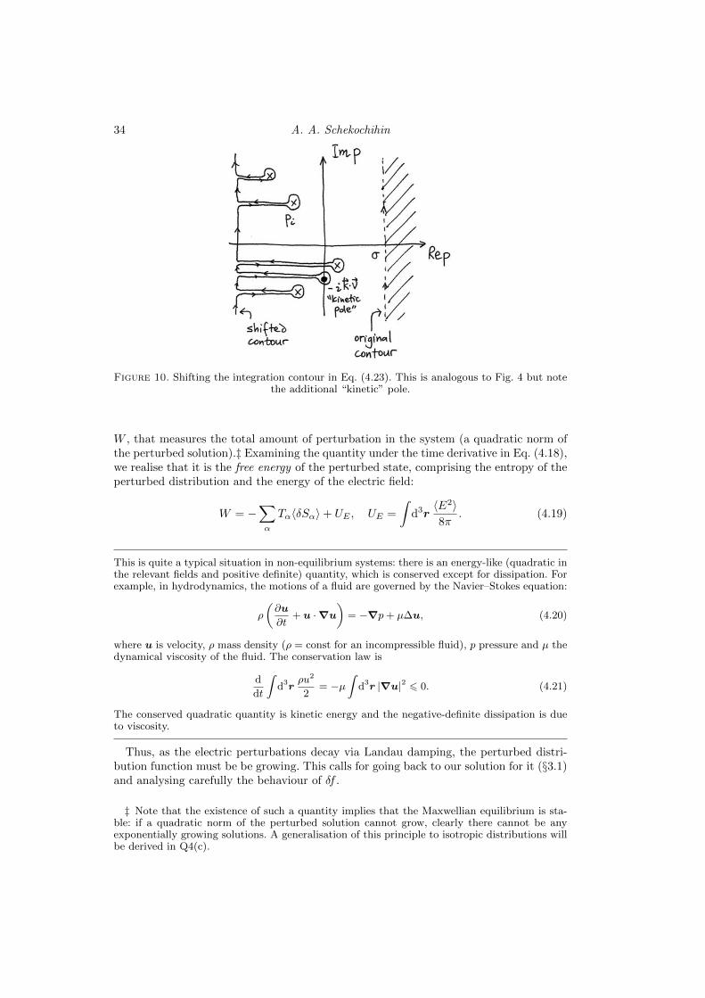
34 A. A. Schekochihin
Figure 10. Shifting the integration contour in Eq. (4.23). This is analogous to Fig. 4 but notethe additional “kinetic” pole.
W , that measures the total amount of perturbation in the system (a quadratic norm ofthe perturbed solution).‡ Examining the quantity under the time derivative in Eq. (4.18),we realise that it is the free energy of the perturbed state, comprising the entropy of theperturbed distribution and the energy of the electric field:
W = −∑α
Tα〈δSα〉+ UE , UE =
∫d3r〈E2〉8π
. (4.19)
This is quite a typical situation in non-equilibrium systems: there is an energy-like (quadratic inthe relevant fields and positive definite) quantity, which is conserved except for dissipation. Forexample, in hydrodynamics, the motions of a fluid are governed by the Navier–Stokes equation:
ρ
(∂u
∂t+ u ·∇u
)= −∇p+ µ∆u, (4.20)
where u is velocity, ρ mass density (ρ = const for an incompressible fluid), p pressure and µ thedynamical viscosity of the fluid. The conservation law is
d
dt
∫d3r
ρu2
2= −µ
∫d3r |∇u|2 6 0. (4.21)
The conserved quadratic quantity is kinetic energy and the negative-definite dissipation is dueto viscosity.
Thus, as the electric perturbations decay via Landau damping, the perturbed distri-bution function must be be growing. This calls for going back to our solution for it (§3.1)and analysing carefully the behaviour of δf .
‡ Note that the existence of such a quantity implies that the Maxwellian equilibrium is sta-ble: if a quadratic norm of the perturbed solution cannot grow, clearly there cannot be anyexponentially growing solutions. A generalisation of this principle to isotropic distributions willbe derived in Q4(c).
Oxford MMathPhys Lecture Notes: Plasma Kinetics and MHD 35
4.3. Structure of the Perturbed Distribution Function
Start with our solution (3.8) for δf(p) and substitute into it the solution (3.15) for ϕ(p):
δf(p) =1
p+ ik · v︸ ︷︷ ︸“kinetic”(ballistic)
pole
iq
m
[∑i
cip− pi︸ ︷︷ ︸
polesrepresenting
linearmodes,
Eq. (3.17)
+ A(p)
]k · ∂f0
∂v+ g
. (4.22)
To compute the inverse Laplace transform, Eq. (3.6), we adopt the same method as in§3.1 (Fig. 4), viz., shift the contour to large negative Re p as shown Fig. 10 and useCauchy’s formula:
δf(t) =1
2πi
∫ i∞+σ
−i∞+σ
dp eptδf(p)
= iq
m
∑i
ciepit
pi + ik · vk · ∂f0
∂v︸ ︷︷ ︸eigenmode-like
solution, comes fromthe poles of ϕ(p)
+ e−ik·vt
[g − i q
m
∑i
cipi + ik · v
k · ∂f0
∂v
]︸ ︷︷ ︸
ballistic response,comes fromp = −ik · v
. (4.23)
Note that the analytical part of ϕ(p) must be A(−ik · v) = 0 in order for the abovesolution to satisfy δf(t = 0) = g.
The solution (4.23) teaches us two important things.
1) Firstly, the Landau-damped solution is not an eigenmode.† Even though the evolu-tion of the potential, Eq. (3.16), does look like a sum of damped eigenmodes of the formϕ ∝ epit, Re pi < 0, the full solution of the Vlasov–Poisson system does not decay: thereis a part of δf(t), the “ballistic response” ∝ e−ik·vt, that oscillates without decaying—infact, we shall see in §4.5 that δf even has a growing part! It is this part that is responsiblefor keeping free energy conserved, as per Eq. (4.18) without collisions. Thus, you maythink of Landau damping as a process of transferring (free) energy from the electric-fieldperturbations to the perturbations of the distribution function,...
2) ...which, and this is the second lesson of Eq. (4.23), have fine structure in velocity(phase) space. This structure gets finer with time: roughly speaking, if δf ∝ e−ikvt, then
1
δf
∂δf
∂v∼ ikt→∞ as t→∞. (4.24)
This phenomenon is called phase mixing. You can think of the basic mechanism respon-sible for it as a shearing in phase space: the homogeneous part of the linearised kineticequation,
∂δf
∂t+ v
∂δf
∂z= . . . , (4.25)
† In contrast, a growing solution (Re pi > 0) can be viewed as an eigenmode because, after afew growth times, the first term in Eq. (4.23) will be exponentially larger than the ballistic term.This will allow us to ignore the latter in our tretament of QLT (§5.1). Note that reversibilityis not an issue for the growing solutions: so, there may be (and often are) damped solutions aswell, so what? We only care about the growing modes because they will be all that is left if wewait long enough.

36 A. A. Schekochihin
Figure 11. Shearing of δf in phase space.
describes advection of δf by a linear shear flow in the the (z, v) plane. This turns any δfstructure in this plane into long thin filaments, with large gradients in v (Fig. 11).
Phase mixing helps us make sense of the notion that, even though ϕ is the velocityintegral of δf , the former can be decaying while the latter is not:
ϕ =4π
k2
∑α
qα
∫d3v δfα︸ ︷︷ ︸fine
structurecancels
∝ e−γt → 0. (4.26)
The velocity integral over the fine structure increasingly cancels as time goes on—aperturbation initially “visible” as ϕ phase-mixes away, disappearing into the negativeentropy associated with the fast velocity dependence of δf [Eq. (4.15)].
4.4. Role of Collisions
As ever larger velocity-space gradients emerge, it becomes inevitable that at some pointthey will become so large that collisions can no longer be ignored. Indeed, the Landaucollision operator is a Fokker–Planck (diffusion) operator in velocity space [Eq. (1.36)]and so it will eventually wipe out the fine structure in v, however small is the collisionfrequency ν. Let us estimate how long it takes.
The size of the velocity-space gradients of δf due to ballistic response is given byEq. (4.24). Then the collision term is(
∂δf
∂t
)c
∼ νv2th
∂2δf
∂v2∼ −νv2
thk2t2δf. (4.27)
Solving for the time evolution of the perturbed distribution function due to collisions,we get
∂δf
∂t∼ −ν(kvtht)
2δf ⇒ δf ∼ exp
(−1
3νk2v2
tht3
). (4.28)
Therefore, the characteristic collisional decay time is
tc ∼1
ν1/3(kvth)2/3. (4.29)
Note that tc ν−1 provided ν kvth, i.e., tc is within the range of times over whichour “collisionless” theory is valid. After time tc, “collisionless” damping becomes irre-versible because the part of δf that is fast-varying in velocity space is lost (entropy hasgrown) and so it is no longer possible, even in principle, to invert all particle trajectories,
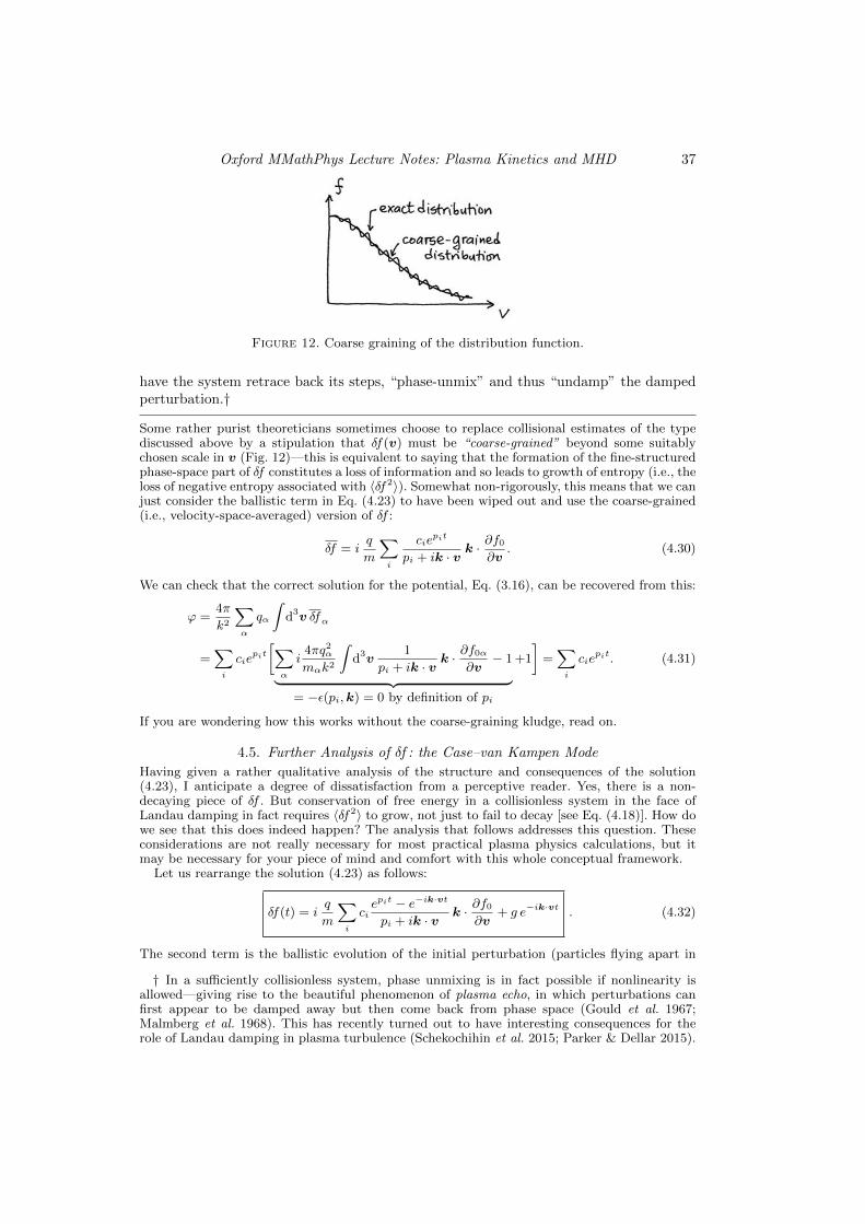
Oxford MMathPhys Lecture Notes: Plasma Kinetics and MHD 37
Figure 12. Coarse graining of the distribution function.
have the system retrace back its steps, “phase-unmix” and thus “undamp” the dampedperturbation.†
Some rather purist theoreticians sometimes choose to replace collisional estimates of the typediscussed above by a stipulation that δf(v) must be “coarse-grained” beyond some suitablychosen scale in v (Fig. 12)—this is equivalent to saying that the formation of the fine-structuredphase-space part of δf constitutes a loss of information and so leads to growth of entropy (i.e., theloss of negative entropy associated with 〈δf2〉). Somewhat non-rigorously, this means that we canjust consider the ballistic term in Eq. (4.23) to have been wiped out and use the coarse-grained(i.e., velocity-space-averaged) version of δf :
δf = iq
m
∑i
ciepit
pi + ik · v k · ∂f0∂v
. (4.30)
We can check that the correct solution for the potential, Eq. (3.16), can be recovered from this:
ϕ =4π
k2
∑α
qα
∫d3v δfα
=∑i
ciepit
[∑α
i4πq2αmαk2
∫d3v
1
pi + ik · v k · ∂f0α∂v− 1︸ ︷︷ ︸
= −ε(pi,k) = 0 by definition of pi
+1
]=∑i
ciepit. (4.31)
If you are wondering how this works without the coarse-graining kludge, read on.
4.5. Further Analysis of δf : the Case–van Kampen Mode
Having given a rather qualitative analysis of the structure and consequences of the solution(4.23), I anticipate a degree of dissatisfaction from a perceptive reader. Yes, there is a non-decaying piece of δf . But conservation of free energy in a collisionless system in the face ofLandau damping in fact requires 〈δf2〉 to grow, not just to fail to decay [see Eq. (4.18)]. How dowe see that this does indeed happen? The analysis that follows addresses this question. Theseconsiderations are not really necessary for most practical plasma physics calculations, but itmay be necessary for your piece of mind and comfort with this whole conceptual framework.
Let us rearrange the solution (4.23) as follows:
δf(t) = iq
m
∑i
ciepit − e−ik·vt
pi + ik · v k · ∂f0∂v
+ g e−ik·vt . (4.32)
The second term is the ballistic evolution of the initial perturbation (particles flying apart in
† In a sufficiently collisionless system, phase unmixing is in fact possible if nonlinearity isallowed—giving rise to the beautiful phenomenon of plasma echo, in which perturbations canfirst appear to be damped away but then come back from phase space (Gould et al. 1967;Malmberg et al. 1968). This has recently turned out to have interesting consequences for therole of Landau damping in plasma turbulence (Schekochihin et al. 2015; Parker & Dellar 2015).

38 A. A. Schekochihin
Figure 13. Emergence of the Case–van Kampen mode.
straight lines at their initial velocities)—the homogeneous solution of the kinetic equation (3.1).This develops a lot of fine-scale velocity-space structure, but obviously does not grow. Thefirst term, the particular solution arising from the (linear) wave-particle interaction, is moreinteresting, especially around the resonances Re pi + k · v = 0.
Consider one of the modes, pi = −iω + γ, and assume γ k · v ∼ ω. This allows us tointroduce “intermediate” times:
1
k · v t 1
γ. (4.33)
This means that the wave has had time to oscillate, phase mixing to develop, but the pertur-bation has not yet been damped away completely. We have then, for the relevant piece of theperturbed distribution (4.32),
δf ∝ epit − e−ik·vt
pi + ik · v = −ie−iωt eγt − e−i(k·v−ω)t
k · v − ω − iγ ≈ −ie−iωt 1− e−i(k·v−ω)t
k · v − ω , (4.34)
with the last, approximate, expression valid at the intermediate times (4.33), assuming alsothat, even though we might be close to the resonance, we shall not come closer than γ, viz.,k · v − ω γ. Respecting this ordering, but taking k · v − ω 1/t, we find
δf ∝ t e−iωt. (4.35)
Thus, δf has a peak that grows with time, emerging from the sea of fine-scale but constant-amplitude structures (Fig. 13). The width of this peak is obviously k · v − ω ∼ 1/t and soδf around the resonance develops a sharp structure, which, in the formal limit t → ∞ (butrespecting γt 1, i.e., with infinitesimal damping), tends to a delta function:
δf ∝ −ie−iωt 1− e−i(k·v−ω)t
k · v − ω → e−iωtπδ(k · v − ω) as t→∞. (4.36)
Here is a “formal” proof:
1− e−ixt
x=
1− cosxt
x︸ ︷︷ ︸finite ast→∞,even atx = 0
+ isinxt
x︸ ︷︷ ︸= it atx = 0
≈ eixt − e−ixt
2x=i
2
∫ t
−tdt′eixt
′→ iπδ(x) as t→∞.
(4.37)The delta-function solution (4.36) is an instance of a Case–van Kampen mode (van Kampen1955; Case 1959).†
If we restore finite damping, we shall see that all this goes on until t ∼ 1/γ, with the delta
† Here we come into passing contact with a whole alternative (to Landau’s) formalism, due tovan Kampen, for treating collisionless plasmas. The objective is more mathematical rigour—but
Oxford MMathPhys Lecture Notes: Plasma Kinetics and MHD 39
function reaching the height ∝ 1/γ and width ∝ γ. In the limit t 1/γ, the damped part ofthe solution decays, eγt → 0, and we are left with just the ballistic part, the second term inEq. (4.23).
Exercise 4.2. Substituting the solution (4.32) into Poisson equation (3.2), confirm directlythat ϕ is given by Eq. (3.16), as it should be, if everything is to be consistent.
4.6. Free-Energy Conservation for a Landau-Damped Solution
Finally, let us convince ourselves that, if we ignore collisions, we can recover Eq. (4.18) with azero right-hand side from the full collisionless Landau-damped solution given by Eqs. (3.16) and(4.32). For simplicity, let us consider just the case of electron Langmuir waves and prove that
d
dt
∫d3v
T |δfk|2
2f0= − d
dt
|Ek|2
8π= −2γk
|Ek|2
8π. (4.38)
Ignoring the term in Eq. (4.32) involving g as it obviously cannot give us a growing amplitude,letting the relevant root of the dispersion relation be pi = −iωpe + γk, where γk is givenby Eq. (3.41), and assuming a Maxwellian f0, we may write the solution (4.32) for electrons(q = −e) as
δfk ≈e
mecie
pit︸ ︷︷ ︸= ϕk
1− e−i(k·v−ipi)t
k · v − ipi2k · vv2the
f0 ≈eϕk
Tk · v 1− e−i(k·v−ωpe)t
k · v − ωpe︸ ︷︷ ︸≈ iπδ(k ·v−ωpe)
f0. (4.39)
We are going to have to compute |δfk|2 and squaring delta functions is a dangerous gamebelonging to the class of games that one must play veeery carefully. Here is how:∣∣∣∣1− e−ixtx
∣∣∣∣2 =1− eixt
x
1− e−ixt
x≈ 1− eixt
x︸ ︷︷ ︸= −it atx = 0
iπδ(x) = tπδ(x). (4.40)
Using this prescription,∫d3v
T |δfk|2
2f0=
∫d3v
e2|ϕk|2
mev2the(k · v)2tπδ(k · v − ωpe)f0
= 2tk2|ϕk|2
8π
ω4pe
k3π
nev2theF(ωpe
k
)︸ ︷︷ ︸= −γk, Eq. (3.41)
= −2γkt|Ek|2
8π. (4.41)
Thus, the entropic part of the free energy grows secularly with time and its time derivativesatisfies Eq. (4.38), q.e.d.
5. Quasilinear Theory
5.1. General Scheme of QLT
We have discussed at length the structure of the linear solution corresponding to aLandau-damped initial perturbation. This could be adequately done for a Maxwellianplasma and we have found that, after some interesting transient time-dependent phase-space dynamics, perturbations damp away and their energy turns into heat, increasingsomewhat the temperature of the equilibrium.
even if this is of limited appeal to you, the book by van Kampen & Felderhof (1967) is still agood read and a good way to reexamine your understanding of how it all works.

40 A. A. Schekochihin
We now consider a different problem: an unstable (and so decidedly non-Maxwellian)equilibrium distribution giving rise to exponentially growing perturbations. The specificexample on which we shall is the bump-on-tail instability, which involves generation ofunstable Langmuir waves with phase velocities corresponding to instances of positivederivative of the equilibrium distribution function (Fig. ??). The energy of the wavesgrows exponentially:
∂|Ek|2
∂t= 2γk|Ek|2, γk =
π
2
ω3pe
k2
1
neF ′(ωpe
k
), (5.1)
where F (vz) =∫
dvx∫
dvy f0(v) [see Eq. (3.41)]. In the absence of collisions, the onlyway for the system to achieve a nontrivial steady state (i.e., such that |Ek|2 is not justzero everywhere) is by adjusting the equilibrium distribution in such a way that
γk = 0 ⇔ F ′(ωpe
k
)= 0 (5.2)
at all k where |Ek|2 6= 0, say, k ∈ [k2, k1]. If we traslate this range into velocities,v = ωpe/k, we see that the equilibrium must develop a flat spot:
F ′(v) = 0 for v ∈ [v1, v2] =
[ωpe
k1,ωpe
k2
]. (5.3)
This is called a quasilinear plateau. Obviously, the rest of the equilibrium distributionmay (and will) also be modified in some, to be determined, way.
These modifications of the original (initial) equilibrium distributions can be accom-plished by the growing fluctuations via the feedback mechanism already discussed in §??,namely, the equilibrium distribution will evolve slowly according to Eq. (2.11):
∂f0
∂t= − q
m
∑k
⟨ϕ∗kik ·
∂δfk∂v
⟩. (5.4)
The general scheme of QLT is—start with an unstable equilibrium f0,—use the linearised Eqs. (3.1) and (3.2) to work out the linear solution for the growingperturbations ϕk and δfk in terms of f0,—use this solution in Eq. (5.4) to evolve f0, leading, if everything works as it is supposedto, to an ever less unstable equilibrium.
Keeping only the fastest growing mode (all others are exponentially small after awhile), the solution (3.16) for the electric perturbations is
ϕk = cke(−iωk+γk)t. (5.5)
In the solution (4.23) for the perturbed distribution function, we may ignore the ballisticterm because the exponentially growing piece (the first term) will eventually leave allthis velocity-space structure behind, so
δfk = iq
m
cke(−iωk+γk)t
−iωk + γk + ik · vk · ∂f0
∂v=
q
m
ϕk
k · v − ωk − iγkk · ∂f0
∂v(5.6)
Substituting the solution (5.6) into Eq. (5.4), we get
∂f0
∂t= − q2
m2
∑k
|ϕk|2ik ·∂
∂v
1
k · v − ωk − iγkk · ∂f0
∂v=
∂
∂v· D(v) · ∂f0
∂v. (5.7)
Oxford MMathPhys Lecture Notes: Plasma Kinetics and MHD 41
This is a diffusion equation in velocity space, with a velocity-dependent diffusion matrix
D(v) = − q2
m2
∑k
ikk|ϕk|21
k · v − ωk − iγk
= − q2
m2
∑k
ikk|ϕk|21
2
(1
k · v − ωk − iγk+
1
−k · v − ω−k − iγ−k︸ ︷︷ ︸here we changedvariables k→ −k
)
= − q2
m2
∑k
kk
k2|Ek|2
i
2
(1
k · v − ωk − iγk− 1
k · v − ωk + iγk
)=
q2
m2
∑k
kk
k2|Ek|2 Im
1
k · v − ωk − iγk
=q2
m2
∑k
kk
k2|Ek|2
γk(k · v − ωk)2 + γ2
k
. (5.8)
To obtain these expressions, we used the fact that the wave-number sum could be over−k as well as over k and that ω−k = −ωk, γ−k = γk (because ϕ−k = ϕ∗k, where ϕk isgiven by Eq. (5.5)). The matrix D is manifestly positive-definite—this adds credence toour a priori expectation that a plateau will form: diffusion will smooth the bump in theequilibrium distribution function.
By way of a consistency check, let us show that Eqs. (5.7–5.8) conserve energy. The rate ofchange of the particle energy assiciated with the equilibrium distribution is
dU0
dt≡ d
dt
∑α
∫∫d3r d3v
mαv2
2f0α =
∑α
∫∫d3r d3v
mαv2
2
∂
∂v· Dα(v) · ∂f0α
∂v
= −∑α
∫∫d3r d3vmαv · Dα(v) · ∂f0α
∂v
= −V∑α
q2αmα
∑k
|Ek|2
k2
∫d3v Im
k · vk · v − ωk − iγk︸ ︷︷ ︸
add and substractωk + iγk in the
numerator
k · ∂f0α∂v
= −V∑k
|Ek|2
4πIm
[(ωk + iγk)
∑α
ω2pα
k21
nα
∫d3v
1
k · v − ωk − iγkk · ∂f0α
∂v︸ ︷︷ ︸= 1− ε(−iωk + γk,k) = 1
because −iωk + iγk is a solution ofdispersion relation ε = 0
]
= −V∑k
2γk|Ek|2
8π= − d
dt
∫d3r
E2
8π, q.e.d., (5.9)
viz., the total energy U0 +∫
d3rE2/8π = const.
5.2. Quasilinear Equations for the Bump-on-Tail Instability in 1D
What follows is the iconic QL calculation due to Vedenov et al. (1962) and Drummond& Pines (1962).
We shall consider electron Langmuir oscillations in 1D, triggered by the bump-on-tail
42 A. A. Schekochihin
instability, so k = kz, ωk = ωpe, γk is given by Eq. (5.1), and the QL diffusion equation(5.7) becomes
∂F
∂t=
∂
∂vD(v)
∂F
∂v, (5.10)
where F (v) is the 1D version of the distribution function, v = vz and the diffusioncoefficient, now a scalar, is given by
D(v) =e2
m2e
∑k
|Ek|2 Im1
kv − ωpe − iγk. (5.11)
5.3. Resonant Region: Spectrum and Plateau
5.4. Energy of Resonant Particles
5.5. Heating of Non-Resonant Particles
5.6. Momentum Conservation
6. Weak Turbulence Theory: Introduction

Oxford MMathPhys Lecture Notes: Plasma Kinetics and MHD 43
Plasma Kinetics Problem Set
1. Industrialised Linear Theory with the Z Function. Consider a two-speciesMaxwellian plasma. Rederive all the results obtained in §§3.4, 3.5, 3.7, 3.8, 3.9 (includingthe exercises) starting from Eq. (3.73) and using the asymptotic expansions (3.80) and(3.81) of the plasma dispersion function.
Namely, consider the limits ζe 1 or ζe 1 and ζi 1, find solutions in theselimits and establish the conditions on the wave number of the perturbations and on theequlibrium parameters under which these solutions are valid.
In particular, for the case of ζe 1 and ζi 1, obtain general expressions for thewave frequency and damping without assuming kλDe to be either small or large. Recoverfrom your solution the cases considered in §§3.7–3.8 and §3.9.
Find also the ion contribution to the damping of the ion acoustic and Langmuir wavesand comment on the circumstances in which it might be important to know what it is.
Convince yourself that you believe the sketch of longitudinal plasma waves in Fig. 9. Ifyou feel computationally inclined, solve the plasma dispersion relation (3.73) numerically[using, e.g., Eq. (3.79)] and see if you can reproduce Fig. 9.
You may wish to check your results against some textbook: e.g., Alexandrov et al.(1984) give a very thorough treatment of the linear theory (although rather in a differentstyle than I did).
2. Transverse plasma waves. Go back to the Vlasov–Maxwell, rather then Vlasov–Poisson, system and consider electromagnetic perturbations in a Maxwellian unmagne-tised plasma (unmagnetised in the sense that in equilibrium, B0 = 0):
∂δfα∂t
+ ik · v δfα +qαmα
(E +
v ×B
c
)· ∂f0α
∂v= 0, (6.1)
where E and B satisfy Maxwell’s equations (1.23–1.26) with charge and current densitiesdetermined by the perturbed distribution function δfα.
(a) Consider an initial-value problem for such perturbations and show that the equationfor the Laplace transform of E can be written in the form†
ε(p,k) · E(p) =
(terms associated with initial
perturbations of δfα, E and B
), (6.2)
where the dielectric tensor ε(p,k) is, in tensor notation,
εij(p,k) =
(δij −
kikjk2
)εTT(p, k) +
kikjk2
εLL(p, k) (6.3)
and the longitudinal dielectric function εLL(p, k) is the familiar electrostatic one, givenby Eq. (3.73), while the transverse dielectric function is
εTT(p, k) = 1 +1
p2
[k2c2 −
∑α
ω2pαζαZ(ζα)
]. (6.4)
† In Q3, dealing with the Weibel instability, you will have to do essentially the same calcu-lation, but with a non-Maxwellian equilibrium. To avoid doing the work twice, you may wishto do that question first and then specialise to a Maxwellian f0α. However, the algebra is a bithairier for the non-Maxwellian case, so it may be useful to do the simpler case first, to trainyour hand—and also to have a way to cross-check the later calculation.

44 A. A. Schekochihin
(b) Hence solve the transverse dispersion relation, εTT(p, k) = 0, and show that, in thehigh-frequency limit (|ζe| 1), the resulting waves are simply the light waves that, atlong wave lengths, turn into plasma oscillations. What is the wave length above whichlight can “feel” that it is propagating through plasma?—this is called the plasma (elec-tron) skin depth, de. Are these waves damped?
(c) In the low-frequency limit (|ζe| 1), show that perturbations are aperiodic (havezero frequency) and damped. Find their damping rate and show that this result is valid forperturbations with wave lengths longer than the plasma skin depth (kde 1). Explainphysically why these perturbations fail to propagate.
3. Weibel instability. Weibel (1958) realised that transverse plasma perturbations cango unstable if the equilibrium distribution is anisotropic with respect to some specialdirection n, namely if f0α = f0α(v⊥, v‖), where v‖ = v · n, v⊥ = |v⊥| and v⊥ =v−v‖n. The anisotropy can be due to some beam or stream of particles injected into theplasma, it also arises in collisionless shocks or, generically, when plasma is sheared or non-isotropically compressed by some external force. The simplest model for an anisotropicdistribution of the required type is a bi-Maxwellian:
f0α =nα
π3/2v2th⊥αvth‖α
exp
(− v2
⊥v2
th⊥α−
v2‖
v2th‖α
), (6.5)
where, formally, vth⊥α =√
2T⊥α/mα and vth‖α =√
2T‖α/mα are the two “thermalspeeds” in a plasma characterised by two effective temperatures T⊥α and T‖α (for eachspecies).
(a) Using exactly the same method as in Q2, consider electromagnetic perturbationsin a bi-Maxwellian plasma, assuming their wave vectors to be parallel to the directionof anisotropy, k ‖ n. Show that the dielectric tensor again has the form (6.3) and thelongitudial dielectric function is again given by Eq. (3.73), while the transverse dielectricfunction is
εTT(p, k) = 1 +1
p2
[k2c2 +
∑α
ω2pα
(1− T⊥α
T‖α[1 + ζαZ(ζα)]
)]. (6.6)
(b) Show that in one of the tractable asymptotic limits, this dispersion relation has azero-frequency, purely growing solution with the growth rate
γ =kvth‖e√
π
T‖e
T⊥e
(∆e − k2d2
e
), (6.7)
where ∆e = T⊥e/T‖e−1 is the fractional temperature anisotropy, which must be positivein order for the instability to occur. Find the maximum growth rate and the correspondingwave number. Under what condition(s) is the asymptotic limit in which you workedindeed a valid approximation for this solution?
(c) Are there any other unstable solutions? (cf. Weibel 1958)
(d) What happens if the electrons are isotropic but ions are not?
(e∗∗) If you want a challenge and a test of stamina, work out the case of perturbationswhose wave number is not necessarily in the direction of the anisotropy (k× n 6= 0). Arethe k ‖ n or some oblique perturbations the fastest growing? This is a lot of algebra,so only do it if you enjoy this sort of thing. The dispersion relation for this general case

Oxford MMathPhys Lecture Notes: Plasma Kinetics and MHD 45
appears to be in the Appendix of Ruyer et al. (2015), but they only solve it numerically;no one seems to have looked at asymptotic limits. This could be the start of a dissertation.
4. Free energy. (a) Starting from the linearised Vlasov–Poisson system and assuminga Maxwellian equilibrium, show by direct calculation from the equations, rather then viaexpansion of the entropy function and the use of energy conservation (as was done in§4.2), that free energy is conserved:
d
dt
∫d3r
[∑α
∫d3v
Tαδf2α
2f0α+|∇ϕ|2
8π
]= 0. (6.8)
This is an exercise in integrating by parts.
(b) Now consider the full Vlasov–Maxwell equations and prove, again for a Maxwellianplasma plus small perturbations,
d
dt
∫d3r
[∑α
∫d3v
Tαδf2α
2f0α+|E|2 + |B|2
8π
]= 0 . (6.9)
(c) Consider the same problem, this time with an equilibrium that is not Maxwellian,but merely isotropic, i.e., f0α = f0α(v), or, in what will prove to be a more convenientform,
f0α = f0α(εα), (6.10)
where εα = mαv2/2 is the particle energy. Find an integral quantity quadratic in per-
turbed fields and distributions that is conserved by the Vlasov–Maxwell system underthese circumstances and that turns into the free energy (6.9) in the case of a Maxwellianequilibrium (e.g., Davidson 1983). Argue that
∂f0α
∂εα< 0 (6.11)
is a sufficient condition for stability of small perturbations in such a plasma.
5.∗ Fluctuation-dissipation relation for a collisionless plasma. Let us consider alinear kinetic system in which perturbations are stirred up by an external force, which wecan think of as an imposed (time-dependent) electric field Eext = −∇χ. The perturbeddistribution function then satisfies
∂δfα∂t
+ v ·∇δfα −qαmα
(∇ϕtot) ·∂f0α
∂v= 0, (6.12)
where ϕtot = ϕ+ χ is the total potential, whose self-consistent part, ϕ, obeys the usualPoisson equation
−∇2ϕ = 4π∑α
qα
∫d3v δfα (6.13)
and the equilibrium f0α is assumed to be Maxwellian.
(a) By considering an initial-value problem for Eqs. (6.12) and (6.13) with zero initialperturbation, show that the Laplace transforms of ϕtot and χ are related by
ϕtot(p) =χ(p)
ε(p), (6.14)
where ε(p) is the dielectric function given by (3.73).

46 A. A. Schekochihin
(b) Consider a time-periodic external force,
χ(t) = χ0e−iω0t. (6.15)
Working out the relevant Laplace transforms and their inverses [see Eq. (3.14)], showthat, after transients have decayed, the total electric field in the system will oscillate atthe same frequency as the external force and be given by
ϕtot(t) =χ0 e
−iω0t
ε(−iω0). (6.16)
(c) Now consider the plasma-kinetic Langevin problem: assume the external force tobe a white noise, i.e., a random process with the time-correlation function
〈χ(t)χ∗(t′)〉 = 2D δ(t− t′). (6.17)
Show that the resulting steady-state mean-square fluctuation level in the plasma will be
〈|ϕtot(t)|2〉 =D
π
∫ +∞
−∞
dω
|ε(−iω)|2. (6.18)
This is a kinetic fluctuation-dissipation relation: given a certain level of external stirring,parametrised by D, this formula predicts the fluctuation energy in terms of D and of theinternal dissipative properties of the plasma, encoded by its dielectric function.
(d) For a system in which the Landau damping is weak, |γ| kvthα, calculate theintegral (6.18) using Plemelj’s formula (3.25) to show that
〈|ϕtot(t)|2〉 = D∑i
1
|γi|
[∂ Re ε(−iω)
∂ω
]−2
ω=ωi
, (6.19)
where pi = −iωi + γi are the weak-damping roots of the dispersion relation.
Here is a reminder of how the standard Langevin problem is solved using Laplace transforms.The Langevin equation is
∂ϕ
∂t+ γϕ = χ(t) , (6.20)
where ϕ describes some quantity, e.g., the velocity of a Brownian particle, subject to a dampingrate γ and an external force χ. In the case of a Brownian particle, χ is assumed to be a whitenoise, as per Eq. (6.17). Assuming ϕ(t = 0) = 0, the Laplace-trasform solution of Eq. (6.20) is
ϕ(p) =χ(p)
p+ γ. (6.21)
Considering first a non-random oscillatory force (6.15), we have
χ(p) =
∫ ∞0
dt e−ptχ(t) =χ0
p+ iω0⇒ ϕ(p) =
χ0
(p+ γ)(p+ iω0). (6.22)
The inverse Laplace transform of ϕ is calculated by shifting the integration contour to largenegative Re p while not allowing it to cross the two poles, p = −γ and p = −iω0, in a manneranalogous to that explained in §3.1 (Fig. 4) and shown in Fig. 14. The integral is then dominatedby the contributions from the poles:
ϕ(t) =1
2πi
∫ i∞+σ
−i∞+σ
dp eptϕ(p) = χ0
(e−iω0t
−iω0 + γ+
e−γt
−γ + iω0
)→ χ0 e
−iω0t
−iω0 + γas t→∞,
(6.23)which is quite obviously the right solution of Eq. (6.20) with a periodic force (the second termin the brackets is the decaying transient needed to enforce the zero initial condition).
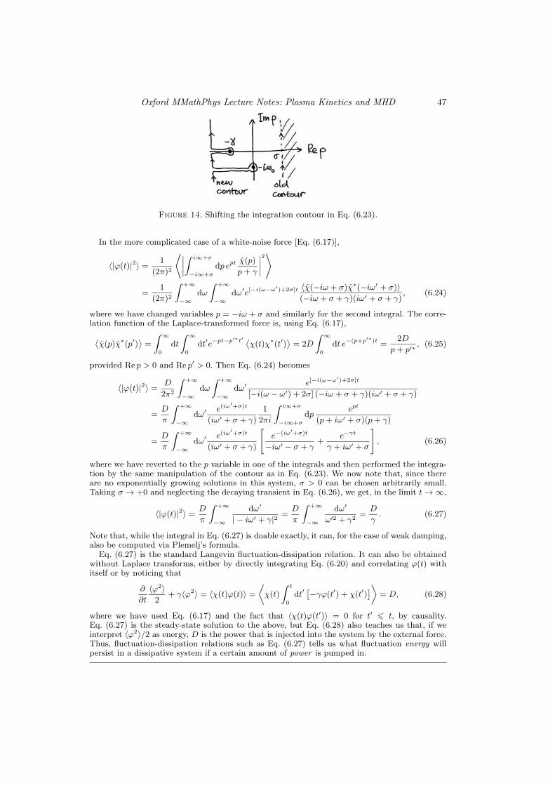
Oxford MMathPhys Lecture Notes: Plasma Kinetics and MHD 47
Figure 14. Shifting the integration contour in Eq. (6.23).
In the more complicated case of a white-noise force [Eq. (6.17)],
〈|ϕ(t)|2〉 =1
(2π)2
⟨∣∣∣∣∫ i∞+σ
−i∞+σ
dp eptχ(p)
p+ γ
∣∣∣∣2⟩
=1
(2π)2
∫ +∞
−∞dω
∫ +∞
−∞dω′e[−i(ω−ω
′)+2σ]t 〈χ(−iω + σ)χ∗(−iω′ + σ)〉(−iω + σ + γ)(iω′ + σ + γ)
, (6.24)
where we have changed variables p = −iω + σ and similarly for the second integral. The corre-lation function of the Laplace-transformed force is, using Eq. (6.17),⟨χ(p)χ∗(p′)
⟩=
∫ ∞0
dt
∫ ∞0
dt′e−pt−p′∗t′ ⟨χ(t)χ∗(t′)
⟩= 2D
∫ ∞0
dt e−(p+p′∗)t =2D
p+ p′∗, (6.25)
provided Re p > 0 and Re p′ > 0. Then Eq. (6.24) becomes
〈|ϕ(t)|2〉 =D
2π2
∫ +∞
−∞dω
∫ +∞
−∞dω′
e[−i(ω−ω′)+2σ]t
[−i(ω − ω′) + 2σ] (−iω + σ + γ)(iω′ + σ + γ)
=D
π
∫ +∞
−∞dω′
e(iω′+σ)t
(iω′ + σ + γ)
1
2πi
∫ i∞+σ
−i∞+σ
dpept
(p+ iω′ + σ)(p+ γ)
=D
π
∫ +∞
−∞dω′
e(iω′+σ)t
(iω′ + σ + γ)
[e−(iω′+σ)t
−iω′ − σ + γ+
e−γt
γ + iω′ + σ
], (6.26)
where we have reverted to the p variable in one of the integrals and then performed the integra-tion by the same manipulation of the contour as in Eq. (6.23). We now note that, since thereare no exponentially growing solutions in this system, σ > 0 can be chosen arbitrarily small.Taking σ → +0 and neglecting the decaying transient in Eq. (6.26), we get, in the limit t→∞,
〈|ϕ(t)|2〉 =D
π
∫ +∞
−∞
dω′
| − iω′ + γ|2 =D
π
∫ +∞
−∞
dω′
ω′2 + γ2=D
γ. (6.27)
Note that, while the integral in Eq. (6.27) is doable exactly, it can, for the case of weak damping,also be computed via Plemelj’s formula.
Eq. (6.27) is the standard Langevin fluctuation-dissipation relation. It can also be obtainedwithout Laplace transforms, either by directly integrating Eq. (6.20) and correlating ϕ(t) withitself or by noticing that
∂
∂t
〈ϕ2〉2
+ γ〈ϕ2〉 = 〈χ(t)ϕ(t)〉 =
⟨χ(t)
∫ t
0
dt′[−γϕ(t′) + χ(t′)
]⟩= D, (6.28)
where we have used Eq. (6.17) and the fact that 〈χ(t)ϕ(t′)〉 = 0 for t′ 6 t, by causality.Eq. (6.27) is the steady-state solution to the above, but Eq. (6.28) also teaches us that, if weinterpret 〈ϕ2〉/2 as energy, D is the power that is injected into the system by the external force.Thus, fluctuation-dissipation relations such as Eq. (6.27) tells us what fluctuation energy willpersist in a dissipative system if a certain amount of power is pumped in.

48 A. A. Schekochihin
6.∗ Phase-mixing spectrum. Here we study the velocity-space structure of the per-turbed distribution function δf derived in Q5.
In order to do this, we need to review the Hermite transform:
δfm =1
n
∫dvz
Hm(u)δf(vz)√2mm!
, u =vzvth
, Hm(u) = (−1)meu2 dm
dume−u
2
, (6.29)
where Hm is the Hermite polynomial of (integer) order m. We are only concerned with the vzdependence of δf (where z, as always, is along the wave number of the perturbations—in thiscase set by the wave number of the force); all vx and vy dependence is Maxwellian and can beintegrated out. The inverse transform is given by
δf(vz) =
∞∑m=0
Hm(u)F (vz)√2mm!
δfm, F (vz) =n√π vth
e−u2
. (6.30)
Because Hm(u) are orthogonal polynomials, viz.,
1
n
∫dvz
Hm(u)Hm′(u)
2mm!F (vz) = δmm′ , (6.31)
they have a Parseval theorem and so the contribution of the perturbed distribution function tothe free energy [Eq. (4.18)] can be written as∫
d3vT |δf |2
2f0=nT
2
∑m
|δfm|2. (6.32)
In a plasma where perturbations are constantly stirred up by a force, Landau damping mustbe operating all the time, removing energy from ϕ to provide “dissipation” of the injectedpower. The process of phase mixing that accompanies Landau damping must then lead to acertain fluctuation level 〈|δfm|2〉 in the Hermite moments of δf . Higher m’s correspond to finerstructure in velocity space: indeed, for m 1, the Hermite polynomials can be approximatedby trigonometric functions,
Hm(u) ≈√
2
(2m
e
)m/2cos(√
2mu− πm
2
)eu
2/2, (6.33)
and so the Hermite transform is somewhat analogous to a Fourier transform in velocity spacewith “frequency”
√2m/vth.
(a) Show that in the kinetic Langevin problem described in Q5(c), the mean squarefluctuation level of the m-th Hermite moment of the perturbed distribution function isgiven by ⟨
|δfm(t)|2⟩
=q2D
T 2π2mm!
∫ +∞
−∞dω
∣∣∣∣ζZ(m)(ζ)
ε(−iω)
∣∣∣∣2 , ζ =ω
kvth, (6.34)
where Z(m)(ζ) is the m-th derivative of the plasma dispersion function [note Eq. (3.82)].
(b∗∗) Show that, assuming m 1 and ζ √
2m,
Z(m)(ζ) ≈√
2π im+1
(2m
e
)m/2eiζ√
2m−ζ2/2 (6.35)
and, therefore, that ⟨|δfm(t)|2
⟩≈ const√
m. (6.36)
Thus, the Hermite spectrum of the free energy is shallow and, in particular, the totalfree energy diverges—it has to be regularised by collisions. This is a manifestation of acopious amount of fine-scale structure in velocity space.
Oxford MMathPhys Lecture Notes: Plasma Kinetics and MHD 49
Deriving Eq. (6.35) is a (reasonably hard) mathematical exercise: it involves using Eqs. (3.82)and (6.33) and manipulating contours in the complex plane. This is a treat for those who likethis sort of thing. Getting to Eq. (6.36) will also require the use of Stirling’s formula.
The Hermite order at which the spectrum (6.36) must be cut off due to collisions can be quicklydeduced as follows. We saw in §4.4 that the typical velocity derivative of δf can be estimatedaccording to Eq. (4.24) and the time it takes for this perturbation to be wiped out by collisionsis given by Eq. (4.29). But, in view of Eq. (6.33), the velocity gradients probed by the Hermite
moment m are of order√
2m/vth. The collisional cut off mc in Hermite space can then beestimated so:
mc ∼ v2th∂2
∂v2∼ (kvthtc)
2 ∼(kvthν
)2/3
. (6.37)
Therefore, the total free energy stored in phase space diverges: using Eqs. (6.32) and (6.36),
1
n
∫d3v
δf2
2f0=
1
2
∑m
⟨|δfm|2
⟩∼∫ mc
dmconst√m∝ ν−1/3 →∞ as ν → +0. (6.38)
In contrast, the total free-energy dissipation rate is finite, however small is the collision frequency:estimating the right-hand side of Eq. (4.18), we get
1
n
∫d3v
δf
f0
(∂δf
∂t
)c
∼ −ν∑m
m⟨|δfm|2
⟩∝ ν
∫ mc
dm√m ∼ kvth. (6.39)
Thus, the kinetic system can collisionally produce entropy at a rate that is entirely independentof the collision frequency.
If you find phase-space turbulence and generally life in Hermite space as fascinating as I do,you can learn more from Kanekar et al. (2015) (on fluctuation-dissipation relations and Hermitespectra) and from Schekochihin et al. (2015) (on what happens when a nonlinearity strikes).
7. Quasilinear theory for the Weibel instability. (a) Starting from the Vlasov equa-tions including magnetic perturbations, show that the slow evolution of the equilibriumdistribution function is described by the following diffusion equation:
∂f0
∂t=
∂
∂v· D(v) · ∂f0
∂v, (6.40)
where the QL diffusion tensor is
D(v) =q2
m2
∑k
1
i(k · v − ωk) + γk
(E∗k +
v ×B∗kc
)(Ek +
v ×Bk
c
)(6.41)
and ωk and γk are the frequency and the growth rate, respectively, of the fastest-growingmode.
(b) Consider the example of the low-frequency electron Weibel instability with wavenumbers k parallel to the anisotropy direction [Eq. (6.7)]. Take k = kz and Bk = Bkyand, denoting Ωk = eBk/mec (the Larmor frequency associated with the perturbedmagnetic field), show that Eq. (6.40) becomes
∂f0
∂t=
∂
∂vx
(Dxx
∂f0
∂vx+Dxz
∂f0
∂vz
)+
∂
∂vzDzz
∂f0
∂vz, (6.42)
where the coefficients of the QL diffusion tensor are
Dxx =∑k
γkk2|Ωk|2, Dxz = −
∑k
2γkvxvzk2v2
z + γ2k
|Ωk|2, Dzz =∑k
γkv2x
k2v2z + γ2
k
|Ωk|2.
(6.43)

50 A. A. Schekochihin
(c) Suppose the electron distribution function f0 is initially bi-Maxwellian, Eq. (6.5),with 0 < T⊥/T‖ − 1 1 (as should be the case for this instability to work). As QLevolution starts, we may define the temperatures of the evolving distribution according to
T⊥ =1
n
∫d3v
m(v2x + v2
y)
2f0, T‖ =
1
n
∫d3vmv2
zf0. (6.44)
Show that initially, viz., before f0 has time to change shape significantly so as no longerto be representable as a bi-Maxwellian, the two temperatures will evolve approximately(using γk kvth) according to†
∂T⊥∂t
= −λT⊥,∂T‖
∂t= 2λT⊥ , where λ(T⊥, T‖) =
∑k
2γk|Ωk|2
k2v2th‖
. (6.45)
Thus, QL evolution will lead, at least initially, to the reduction of the temperatureanisotropy, thus weaking the instability (these equations should not be used to traceT⊥/T‖ − 1 all the way to zero because there is no reason why the QL evolution shouldpreserve the bi-Maxwellian shape of f0).
Note that, even modulo the caveat about the bi-Maxwellian not being a long-term solution,this does not give us a way to estimate (or even guess) what the saturated fluctuation levelwill be. The standard Weibel lore is that saturation occurs when the approximations that wereused to derive the linear theory (Q3) break down, namely, when magnetic field becomes strongenough to magnetise the plasma, rendering the Larmor scale ρe = vthe/Ωk associated with thefluctuations small enough to be comparable to the latter’s wavelengths ∼ k−1. Using the typicalvalues of k from Eq. (6.7), we can write this condition as follows
Ωk ∼ kvthe ∼√
∆evthede
⇔ 1
βe≡ B2/8π
neTe∼ ∆e . (6.46)
Thus, Weibel instability will produce fluctuations the ratio of whose magnetic-energy densityto the electron-thermal-energy density (customarily referred to as the inverse of “plasma beta,”1/βe) is comparable to the electron pressure anisotropy ∆e. Because at that point the fluctu-ations will be relaxing this pressure anisotropy at the same rate as they can grow in the firstplace [in Eq. (6.45), λ ∼ γk], the QL approach is not really valid anymore.
These considerations are, however, usually assumed to be qualitatively sound and lead peopleto believe that, even in collisionless plasmas, the anisotropy of the electron distribution must belargely self-regulating, with unstable Weibel fluctuations engendered by the anisotropy quicklyacting to isotropise the plasma (or at least the electrons).
This is all currently very topical in the part of the plasma astrophysics world preoccupiedwith collisionless shocks, origin of the cosmic magnetism, hot weakly collisional environmentssuch as the intergalactic medium (in galaxy clusters) or accretion flows around black holes andmany other interesting subjects.
IUCUNDI ACTI LABORES.
† These equations say that the total mean kinetic energy,∫
d3v (mv2/2)f0 = n(T⊥ + T‖/2),does not change. But fluctuations are generated and grow at the rate γk! Without much furtheralgebra, can you tell whether you should therefore doubt the result (6.45)?
Oxford MMathPhys Lecture Notes: Plasma Kinetics and MHD 51
PART II
Magnetohydrodynamics
7. MHD Equations
7.1. Conservation of Mass
7.2. Conservation of Momentum
7.3. Electromagnetic Fields and Forces
7.4. Maxwell Stress and Magnetic Forces
7.5. Evolution of Magnetic Field
7.6. Magnetic Reynolds Number
7.7. Lundquist Theorem
7.8. Flux Freezing
7.9. Amplification of Magnetic Field by Fluid Flow
7.10. Conservation of Energy
7.11. Lagrangian MHD
7.12. MHD Action Principle
8. MHD Dynamo

52 A. A. Schekochihin
9. MHD in a Straight Magnetic Field
9.1. MHD Waves
9.1.1. Alfven Waves
9.1.2. Magnetosonic Waves
9.1.3. Parallel Propagation
9.1.4. Perpendicular Propagation
9.1.5. Anisotropic Perturbations
9.1.6. High-β Limit
9.2. Incompressible MHD
9.2.1. Subsonic Ordering
9.2.2. Incompressible MHD Equations
9.2.3. Elsasser MHD
9.2.4. Cross-Helicity
9.3. Reduced MHD
9.3.1. Alfvenic Perturbations
9.3.2. Compressive Perturbations
9.3.3. Elsasser Fields and Energetics of RMHD
9.3.4. Entropy Mode
10. MHD Turbulence

Oxford MMathPhys Lecture Notes: Plasma Kinetics and MHD 53
11. MHD Relaxation
11.1. Static MHD Equilibria
11.1.1. MHD Equilibria in Cylindrical Geometry
11.1.2. Force-Free Equilibria
11.2. Helicity
11.3. J. B. Taylor Relaxation
11.4. Relaxed State of a Cylindrical Pinch
12. MHD Stability and Instabilities
12.1. Energy Principle
12.2. Explicit Calculation of δW2
12.2.1. Linearised MHD Equations
12.2.2. Energy Perturbation
12.3. Interchange Instabilities
12.4. Instabilities of a Pinch
12.4.1. Sausage Instability
12.4.2. Kink Instabilities
13. Resistive MHD: Magnetic Reconnection
13.1. Tearing Mode
13.2. Sweet–Parker Reconnection
13.3. Plasmoid Instability
13.4. Plasmoid Reconnection

54 A. A. Schekochihin
Acknowledgments
I am grateful to many at Oxford who have given advice, commented, pointed out er-rors, asked challenging questions and generally helped me get a grip. Particular thanksto Andre Lukas and Fabian Essler, who were comrades in arms in the creation of theMMathPhys (led by Andre), to Paul Dellar and James Binney, with whom I have collab-orated on teaching Kinetic Theory and MHD, and to Felix Parra, Michael Barnes andPeter Norreys, who have helped design a coherent sequence of courses on plasma physics.I am also grateful to F. Rincon and F. Califano, for some help with plasma instabilities.
REFERENCES
Adams, D. 1979 The Hitch-Hikers Guide to the Galaxy . London: Pan Books.
Alexandrov, A. F., Bogdankevich, L. S. & Rukhadze, A. A. 1984 Principles of PlasmaElectrodynamics. Springer.
Balescu, R. 1963 Statistical Mechanics of Charged Particles. Interscience.
Binney, J. J. 2015 Kinetic Theory of Self-Gravitating Systems. Lecture Notesfor the Oxford MMathPhys course on Kinetic Theory; URL: http://www-thphys.physics.ox.ac.uk/user/JamesBinney/kt.pdf.
Bohm, D. & Gross, E. P. 1949 Theory of plasma oscillations. A. Origin of medium-like be-havior. Phys. Rev. 75, 1851.
Braginskii, S. I. 1965 Transport processes in a plasma. Rev. Plasma Phys. 1, 205.
Buneman, O. 1958 Instability, turbulence, and conductivity in current-carrying plasma. Phys.Rev. Lett. 1, 8.
Case, K. M. 1959 Plasma oscillations. Ann. Phys. (N.Y.) 7, 349.
Chapman, S. & Cowling, T. G. 1991 The Mathematical Theory of Non-Uniform Gases.Cambridge: Cambridge University Press, 3rd Edition.
Davidson, R. C. 1983 Kinetic waves and instabilities in a uniform plasma. In Handbook ofPlasma Physics, Volume 1 (ed. A. A. Galeev & R. N. Sudan), p. 519. Amsterdam: North-Holland.
Dellar, P. J. 2015 Kinetic Theory of Gases. Lecture Notes for the Oxford MMathPhys courseon Kinetic Theory; URL: http://people.maths.ox.ac.uk/dellar/MMPkinetic.html.
Drummond, W. E. & Pines, D. 1962 Nonlinear stability of plasma oscillations. Nucl. FusionSuppl. 3, 1049.
Fried, B. D. & Conte, S. D. 1961 The Plasma Dispersion Function. New York: AcademicPress.
Gould, R. W., O’Neil, T. M. & Malmberg, J. H. 1967 Plasma wave echo. Phys. Rev. Lett.19, 219.
Helander, P. & Sigmar, D. J. 2005 Collisional Transport in Magnetized Plasmas. Cambridge:Cambridge University Press.
Kadomtsev, B. B. 1965 Plasma Turbulence. Academic Press.
Kanekar, A., Schekochihin, A. A., Dorland, W. & Loureiro, N. F. 2015 Fluctuation-dissipation relations for a plasma-kinetic Langevin equation. J. Plasma Phys. 81,305810104.
Klimontovich, Yu. L. 1967 The Statistical Theory of Non-Equilibrium Processes in a Plasma.MIT Press.
Kolmogorov, A. N. 1941 The local structure of turbulence in incompressible viscous fluid atvery large Reynolds numbers. Dokl. Acad. Nauk SSSR 30, 299.
Krommes, J. A. 2015 A tutorial introduction to the statistical theory of turbulent plasmas, ahalf-century after Kadomtsev’s Plasma Turbulence and the resonance-broadening theory ofDupree and Weinstock. J. Plasma Phys. 81, 205810601.
Landau, L. 1936 Transport equation in the case of Coulomb interaction. Zh. Eksp. Teor. Fiz.7, 203.
Landau, L. 1946 On the vibration of the electronic plasma. Zh. Eksp. Teor. Fiz. 16, 574, Englishtranslation in J. Phys. USSR 10, 25 (1946).

Oxford MMathPhys Lecture Notes: Plasma Kinetics and MHD 55
Lifshitz, E. M. & Pitaevskii, L. P. 1981 Physical Kinetics (L. D. Landau and E. M. Lifshitz’sCourse of Theoretical Physics, Volume 10). Elsevier.
Malmberg, J. H., Wharton, C. B., Gould, R. W. & O’Neil, T. M. 1968 Plasma waveecho experiment. Phys. Rev. Lett. 20, 95.
Nazarenko, S. 2011 Wave Turbulence. Springer.Parker, J. T. & Dellar, P. J. 2015 Fourier-Hermite spectral representation for the Vlasov-
Poisson system in the weakly collisional limit. J. Plasma Phys. 81, 305810203.Parra, F. I. 2016a Collisional Plasma Physics. Lecture Notes for the Oxford MMathPhys
course taught in Trinity Term.Parra, F. I. 2016b Collisionless Plasma Physics. Lecture Notes for the Oxford MMathPhys
course taught in Hilary Term.Ruyer, C., Gremillet, L., Debayle, A. & Bonnaud, G. 2015 Nonlinear dynamics of the
ion Weibel-filamentation instability: An analytical model for the evolution of the plasmaand spectral properties. Phys. Plasmas 22, 032102.
Schekochihin, A. A., Parker, J. T., Highcock, E. G., Dellar, P. J., Dorland, W.& Hammett, G. W. 2015 Phase mixing vs. nonlinear advection in drift-kinetic plasmaturbulence. arXiv:1508.05988.
Tonks, L. & Langmuir, I. 1929 Oscillations in ionized gases. Phys. Rev. 33, 195.van Kampen, N. G. 1955 On the theory of stationary waves in plasmas. Physica 9, 949.van Kampen, N. G. & Felderhof, B. U. 1967 Theoretical Methods in Plasma Physics. Am-
sterdam: North-Holland.Vedenov, A. A., Velikhov, E. P. & Sagdeev, R. Z. 1962 Quasi-linear theory of plasma
oscillations. Nucl. Fusion Suppl. 2, 465.Weibel, E. S 1958 Spontaneously growing transverse waves in a plasma due to an anisotropic
velocity distribution. Phys. Rev. Lett. 2, 83.Zakharov, V. E., Lvov, V. S. & Falkovich, G. 1992 Kolmogorov Spectra
of Turbulence I: Wave Turbulence. Springer (updated online version URL:http://lvov.weizmann.ac.il/lvov/Texts-Online/002 KST/002 KST-index.html).

56 A. A. Schekochihin
CONTENTS
1. Kinetic Description of a Plasma 11.1. Quasineutrality 11.2. Weak Interactions 21.3. Debye Shielding 21.4. Micro- and Macroscopic Fields 31.5. Maxwell’s Equations 41.6. Vlasov–Landau Equation 51.7. Collision Operator 61.8. Klimontovich’s Version of BBGKY 71.9. So What’s New and What Now? 8
2. Equilibrium and Fluctuations 102.1. Plasma Frequency 102.2. Slow vs. Fast 112.3. Multiscale Dynamics 112.4. Hierarchy of Approximations 12
3. Linear Theory: Plasma Waves, Landau Damping and Kinetic Instabli-ties 14
3.1. Initial-Value Problem 143.2. Calculating the Dielectric Function: the “Landau Prescription” 173.3. Solving the Dispersion Relation: Slow-Damping/Growth Limit 193.4. Langmuir Waves 203.5. Landau Damping 223.6. Physical Picture of Landau Damping 233.7. Ion-Acoustic Waves 253.8. Damping of Ion-Acoustic Waves and Ion-Acoustic Instability 263.9. Ion Langmuir Waves 273.10. Summary of Electrostatic (Longitudinal) Plasma Waves 283.11. Plasma Dispersion Function: Putting Linear Theory on Industrial Basis 28
4. Energy, Entropy, Free Energy, Heating, Irreversibility and Phase Mix-ing 30
4.1. Energy Conservation and Heating 304.2. Entropy and Free Energy 324.3. Structure of the Perturbed Distribution Function 354.4. Role of Collisions 364.5. Further Analysis of δf : the Case–van Kampen Mode 374.6. Free-Energy Conservation for a Landau-Damped Solution 39
5. Quasilinear Theory 395.1. General Scheme of QLT 395.2. Quasilinear Equations for the Bump-on-Tail Instability in 1D 415.3. Resonant Region: Spectrum and Plateau 425.4. Energy of Resonant Particles 425.5. Heating of Non-Resonant Particles 425.6. Momentum Conservation 42
6. Weak Turbulence Theory: Introduction 427. MHD Equations 51
7.1. Conservation of Mass 517.2. Conservation of Momentum 517.3. Electromagnetic Fields and Forces 51
Oxford MMathPhys Lecture Notes: Plasma Kinetics and MHD 57
7.4. Maxwell Stress and Magnetic Forces 517.5. Evolution of Magnetic Field 517.6. Magnetic Reynolds Number 517.7. Lundquist Theorem 517.8. Flux Freezing 517.9. Amplification of Magnetic Field by Fluid Flow 517.10. Conservation of Energy 517.11. Lagrangian MHD 517.12. MHD Action Principle 51
8. MHD Dynamo 519. MHD in a Straight Magnetic Field 52
9.1. MHD Waves 529.2. Incompressible MHD 529.3. Reduced MHD 52
10.MHD Turbulence 5211.MHD Relaxation 53
11.1. Static MHD Equilibria 5311.2. Helicity 5311.3. J. B. Taylor Relaxation 5311.4. Relaxed State of a Cylindrical Pinch 53
12.MHD Stability and Instabilities 5312.1. Energy Principle 5312.2. Explicit Calculation of δW2 5312.3. Interchange Instabilities 5312.4. Instabilities of a Pinch 53
13.Resistive MHD: Magnetic Reconnection 5313.1. Tearing Mode 5313.2. Sweet–Parker Reconnection 5313.3. Plasmoid Instability 5313.4. Plasmoid Reconnection 53
Related Documents