Lecture CCD.ppt

1

Detectors

RIT Course Number 1051-465Lecture CCDs

2

Aims for this lecture• To describe the basic CCD

– physical principles– operation– and performance of CCDs

• Given modern examples of CCDs

3

CCD Introduction• A CCD is a two-dimensional array of metal-oxide-

semiconductor (MOS) capacitors.

• The charges are stored in the depletion region of the MOS capacitors.

• Charges are moved in the CCD circuit by manipulating the voltages on the gates of the capacitors so as to allow the charge to spill from one capacitor to the next (thus the name “charge-coupled” device).

• An amplifier provides an output voltage that can be processed.

• The CCD is a serial device where charge packets are read one at a time.

4

CCD Physics

5

Semiconductors• A conductor allows for the flow of electrons in the presence of

an electric field.

• An insulator inpedes the flow of electrons.

• A semiconductor becomes a conductor if the electrons are excited to high enough energies, otherwise it is an insulator.– allows for a “switch” which can be on or off– allows for photo-sensitive circuits (photon absorption adds energy to

electron)

• Minimum energy to elevate an electron into conduction is the “band gap energy”

6

• Semiconductors occupy column IV of the Periodic Table• Outer shells have four empty valence states• An outer shell electron can leave the shell if it absorbs

enough energy

Periodic Table

7

Simplified silicon band diagram

Conduction band

Valence band

Eg bandgap 1.24

( )cogE eV

8

Semiconductor Dopants

9

• In a PN junction, positively charged holes diffuse into the n-type material. Likewise, negatively charged electrons diffuse in the the p-type material.

• This process is halted by the resulting E-field.

• The affected volume is known as a “depletion region”.

• The charge distribution in the depletion region is electrically equivalent to a 2-plate capacitor.

PN Junctions

10

Photon detection in PN junctions

• A photon can interact with the semiconductor to create an electron-hole pair.

• The electron will be drawn to the most positively charged zone in the PN junction, located in the depletion region in the n-type material.

• Likewise, the positively charged hole will seek the most negatively charged region.

• Each photon thus removes one unit of charge from the capacitor. This is how photons are detected in both CCDs and most IR arrays.

11

MOS Capacitor Geometry• A Metal-Oxide-Semiconductor (MOS) capacitor has a

potential difference between two metal plates separated by an insulartor.

12

Surface Channel Potential Well

13

Potential in MOS Capacitor

14

CCD Readout

15

“Bucket Brigade”

C:\figerdev\RIT\teaching\Detectors 465 20083\source material\CCDMovieMOD.gif

16

CCD Readout Animation

17

CCD Readout Alternate Animation

18

CCD Readout Architecture Terms

Charge motion

Ch

arg

e m

oti

on

Serial (horizontal) register

Parallel (vertical) registers

Pixel

Image area(exposed to light)

Output amplifier

masked area(not exposed to light)

19

CCD Clocking

20

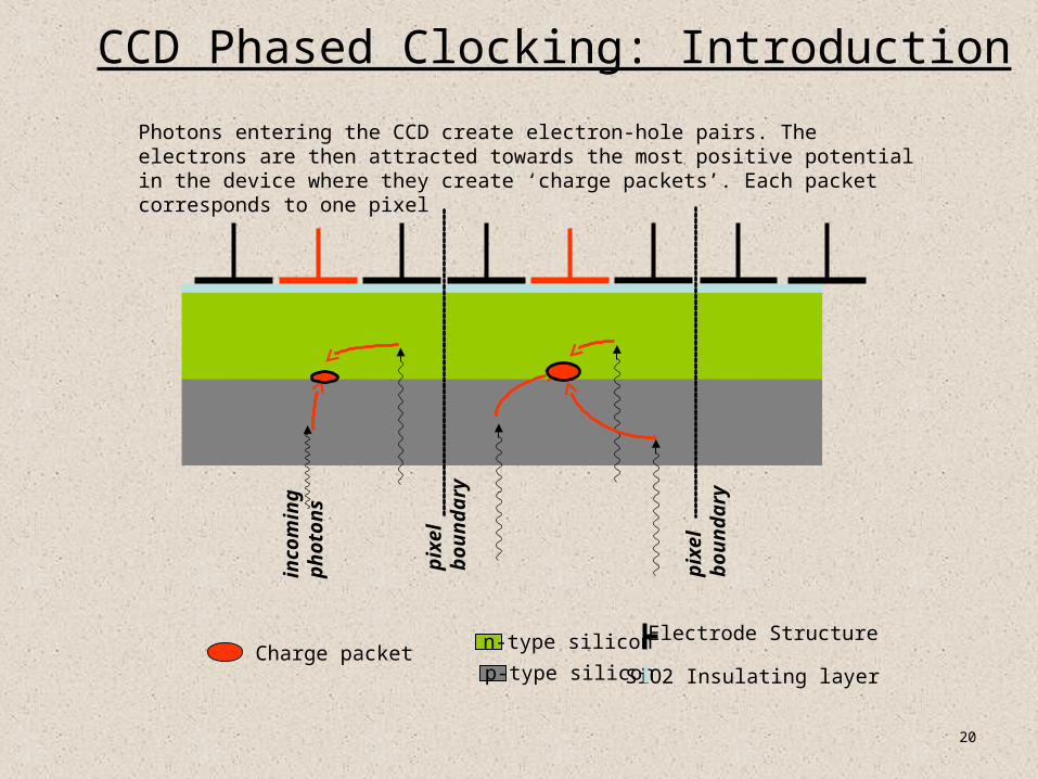
pix

el

bo

un

dar

y

Charge packetp-type silicon

n-type silicon

SiO2 Insulating layer

Electrode Structure

pix

el

bo

un

dar

y

inco

min

gp

ho

ton

s

Photons entering the CCD create electron-hole pairs. The electrons are then attracted towards the most positive potential in the device where they create ‘charge packets’. Each packet corresponds to one pixel

CCD Phased Clocking: Introduction

21

123

Time-slice shown in diagram

+5V

0V

-5V

+5V

0V

-5V

+5V

0V

-5V

1

2

3

CCD Phased Clocking: Step 1

22

123

CCD Phased Clocking: Step 2

+5V

0V

-5V

+5V

0V

-5V

+5V

0V

-5V

1

2

3

23

123

CCD Phased Clocking: Step 3

+5V

0V

-5V

+5V

0V

-5V

+5V

0V

-5V

1

2

3

24

123

CCD Phased Clocking: Step 4

+5V

0V

-5V

+5V

0V

-5V

+5V

0V

-5V

1

2

3

25

123

CCD Phased Clocking: Step 5

+5V

0V

-5V

+5V

0V

-5V

+5V

0V

-5V

1

2

3

26

CCD Phased Clocking: Summary

27

CCD output circuit

28

CCD Readout Layout

29

CCD Readout Device

30

CCD Readout Device Closeup

31

CCD Enhancements

32

Buried channel CCD• Surface channel CCDs shift charge along a thin layer in the

semiconductor that is just below the oxide insulator.

• This layer has crystal irregularities which can trap charge, causing loss of charge and image smear.

• If there is a layer of n-doped silicon above the p-doped layer, and a voltage bias is applied between the layers, the storage region will be deep within the depletion region.

• This is called a buried-channel CCD, and it suffers much less from charge trapping.

34

Buried Channel Potential Well

35

Back Side Illumination• As described to now, the CCDs are illuminated through the

electrodes. Electrodes are semi-transparent, but some losses occur, and they are non-uniform losses, so the sensitivity will vary within one pixel. The “fill factor” will be less than one.

• Solution is to illuminate the CCD from the back side.

• This requires thinning the CCD, either by mechanical machining or chemical etching, to about 15μm.

36

Photon Propogation in Thinned Device

n-type silicon

p-type silicon

Silicon dioxide insulating layerPolysilicon electrodes

Inco

min

g ph

oton

s

625m

n-type silicon

p-type silicon

Silicon dioxide insulating layerPolysilicon electrodes

Inco

min

g ph

oton

s

Anti-reflective (AR) coating

15m

37

Random Walk in Field-Free Thick Device

38

Sweep Field

39

Short QE Improvement from Thinning

40

CCD Performance

41

CCD Performance Categories• Charge generation

Quantum Efficiency (QE), Dark Current

• Charge collection

full well capacity, pixels size, pixel uniformity,

defects, diffusion (Modulation Transfer

Function, MTF)

• Charge transfer

Charge transfer efficiency (CTE),

defects

• Charge detection

Readout Noise (RON), linearity

42

Photon Absorption Length in Si

43

Well Capacity• Well capacity is defined as the maximum charge that can be

held in a pixel.

• “Saturation” is the term that describes when a pixel has accumulated the maximum amount of charge that it can hold.

• The “full well” capacity in a CCD is typically a few hundred thousand electrons per pixel for today’s technologies.

• A rough rule of thumb is that well capacity is about 10,000 electrons/um2.

• The following gives a typical example (for a surface channel CCD).

electrons. 000,240Q pixel, m8m4For

, 740012044.335222

m

e

cm

nCVolts

cm

nFV

A

C

A

Q OX

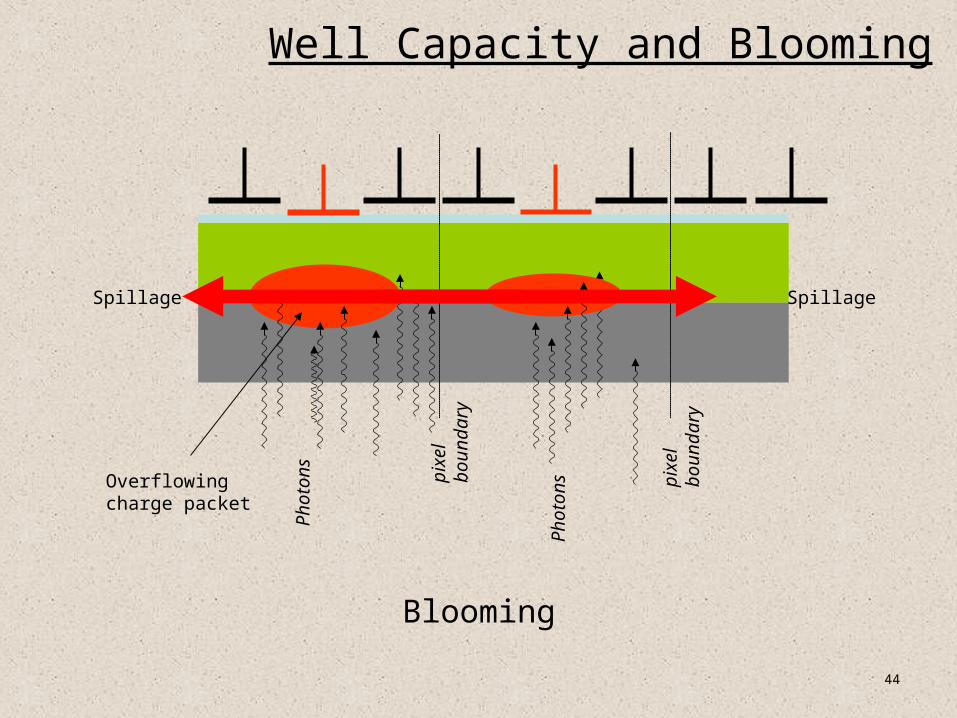
44

Well Capacity and Blooming

Blooming

pixe

l bo

und

ary

Pho

ton

s

Pho

ton

sOverflowingcharge packet

Spillage Spillage

pixe

l bo

und

ary

45

Blooming Example

Bloomed star images

46

Read-Out Noise• Read noise is mainly due to Johnson noise in amplifier.

• This noise can be reduced by reducing the bandwidth, but this requires that readout is slower.

0

2

4

6

8

10

12

14

2 3 4 5 6

Time spent measuring each pixel (microseconds)

Re

ad N

ois

e (

ele

ctro

ns

RM

S)

47

Defects: Dark Columns

Dark columns: caused by ‘traps’ that block the vertical transfer of charge during image readout.

Traps can be caused by crystal boundaries in the silicon of the CCD or by manufacturing defects.

Although they spoil the chip cosmetically, dark columns are not a big problem (removed by calibration).

48

Defects: Bright Columns

Cosmic rays

Cluster ofHot Spots

BrightColumn

Bright columns are also caused by traps . Electrons contained in such traps can leak out during readout causing a vertical streak.

Hot Spots are pixels with higher than normal dark current. Their brightness increases linearly with exposure times

Somewhat rarer are light-emitting defects which are hot spots that act as tiny LEDS and cause a halo of light on the chip.

49

Charge Transfer Efficiency

CTE = Charge Transfer Efficiency (typically 0.9999 to 0.999999)= fraction of electrons transferred from one pixel to the next

CTI = Charge Transfer Inefficiency = 1 – CTE (typically 10– 6 to 10– 4)= fraction of electrons deferred by one pixel or more

Cause of CTI: charges are trapped (and later released) by defects in the silicon crystal lattice

CTE of 0.99999 used to be thought of as pretty good but ….

Think of a 9K x 9K CCD

50

Charge Transfer Efficiency• When the wells are nearly empty, charge can be trapped by

impurities in the silicon. So faint images can have tails in the vertical direction.

• Modern CCDs can have a charge transfer efficiency (CTE) per transfer of 0.9999995, so after 2000 transfers only 0.1% of the charge is lost.

good CTE bad CTE

51

Example: X-ray events with charge smearing in an

irradiated CCD (from GAIA-LU-TN01)

direction of charge transfer

In the simplest picture (“linear CTI”) part of the original image is smeared with an exponentialdecay function, producing “tails”:

original image after n transfers

52

Deferred Charge vs. CTE and Size• Percentage of charge which is really transferred.

• “n” 9s: five 9s = 99.99999%

53

Dark Current• Dark current is generated when thermal effects cause an

electron to move from the valence band to the conduction band.

• The majority of dark current is created near the interface between the Si and the SiO2, where interface states at energy between the valence and conduction bands act as a stepping stone for electrons.

• CCDs can be operated at temperatures of around 140K, to reduce thermal effects.

54

Dark Current vs. Temperature• Thermally generated electrons are indistinguishable from

photo-generated electrons : “Dark Current” (noise)

• Cool the CCD down!!!

1

10

100

1000

10000

-110 -100 -90 -80 -70 -60 -50 -40

Temperature Centigrade

Ele

ctro

ns p

er p

ixel

per

hou

r

55

Linearity and Saturation• Typically the full well capacity of a CCD pixel 25 μm square

is 500,000 electrons. If the charge in the well exceeds about 80% of this value the response will be non-linear. If it exceeds this value charge will spread through the barrier phase to surrounding pixels.

• This charge blooming occurs mainly vertically, as there is little horizontal bleeding because of the permanent doped channel stops.

• Readout register pixels are larger, so there is less saturation effect in the readout register.

56

CCD readout noise• Reset noise: there is a noise associated with recharging the

output storage capacitor, given by σreset= (kTC) where C is the output capacitance in Farads. Surface state noise, due to fast interface states which absorb and release charges on short timescales.

• This is removed by correlated double sampling, where the reset voltage is measured after reset and again after readout. The first value is subtracted from the second, as this voltage will not change.

• The output Field Effect Transistor also contributes noise. This is the ultimate limit to the readout noise, at a level of 2-3 electrons

57

Other noise sources• Fixed pattern noise. The sensitivity of pixels is not the same,

for reasons such as differences in thickness, area of electrodes, doping. However these differences do not change, and can be calibrated out by dividing by a flat field, which is an exposure of a uniform light source.

• Bias noise. The bias voltage applied to the substrate causes an offset in the signal, which can vary from pixel to pixel. This can be removed by subtracting the average of a number of bias frames, which are readouts of zero exposure frames. Modern CCDs rarely display any fixed pattern bias noise.

58

Interference Fringes• In thinned CCDs there are interference effects caused by

multiple reflections within the silicon layer, or within the resin which holds the CCD to a glass plate to flatten it.

• These effects are classical thin film interference (Newton’s rings).

• Only visible if there is strong line radiation in the passband, either in the object or in the sky background.

• Visible in the sky at wavelengths > 700nm.

• Corrected by dividing by a scaled exposure of blank sky.

59

Examples of fringing

Fringing on H1RG SiPIN device at 980nm

60

CCD Examples

61

First astronomical CCD image

1974 on an 8” telescope

62

CCD in a Dual-Inline Package

63

CCDs and mosaics

4096 x 2048 3 edge buttable CCD Canada-France-Hawaii telescope 12k x8k mosaic

64

MegaCam

40 CCDs, 377 Mpixels, CFHT

65

HST/WFC3

66

CCD Science Applications

67

68

Large CCD Mosaics

69

The LSST Camera

70

The LSST Focal Plane

Guide Sensors (8 locations)

Wavefront Sensors (4 locations)

3.5 degree Field of View (634 mm diameter)