3 Aaron Clauset @aaronclauset Assistant Professor of Computer Science University of Colorado Boulder External Faculty, Santa Fe Institute Lecture 6 (supplemental): Stochastic Block Models © 2017 Aaron Clauset

Welcome message from author
This document is posted to help you gain knowledge. Please leave a comment to let me know what you think about it! Share it to your friends and learn new things together.
Transcript
100150
200250
300
Aaron Clauset @aaronclausetAssistant Professor of Computer ScienceUniversity of Colorado BoulderExternal Faculty, Santa Fe Institute
Lecture 6 (supplemental):Stochastic Block Models
© 2017 Aaron Clauset

what is structure?

• makes data different from noise makes a network different from a random graph
what is structure?
• makes data different from noise makes a network different from a random graph
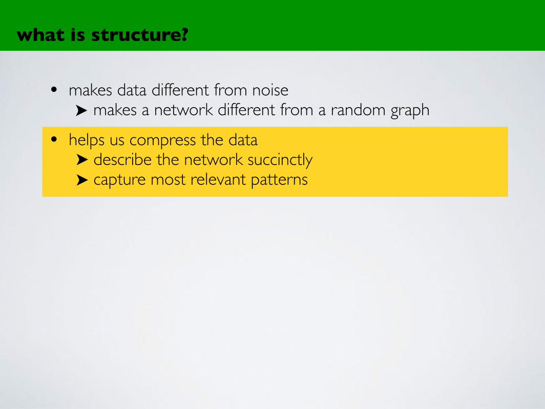
• helps us compress the data describe the network succinctly capture most relevant patterns
what is structure?
• makes data different from noise makes a network different from a random graph
• helps us compress the data describe the network succinctly capture most relevant patterns
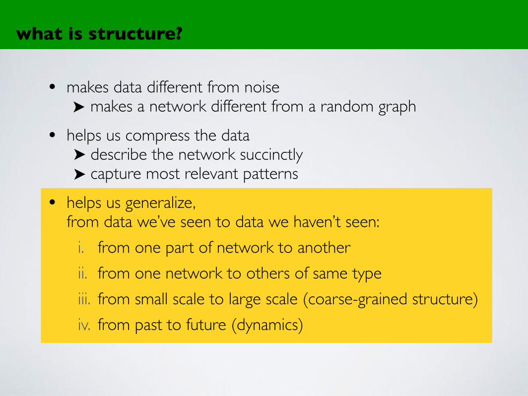
• helps us generalize, from data we’ve seen to data we haven’t seen:
i. from one part of network to anotherii. from one network to others of same typeiii. from small scale to large scale (coarse-grained structure)iv. from past to future (dynamics)
what is structure?
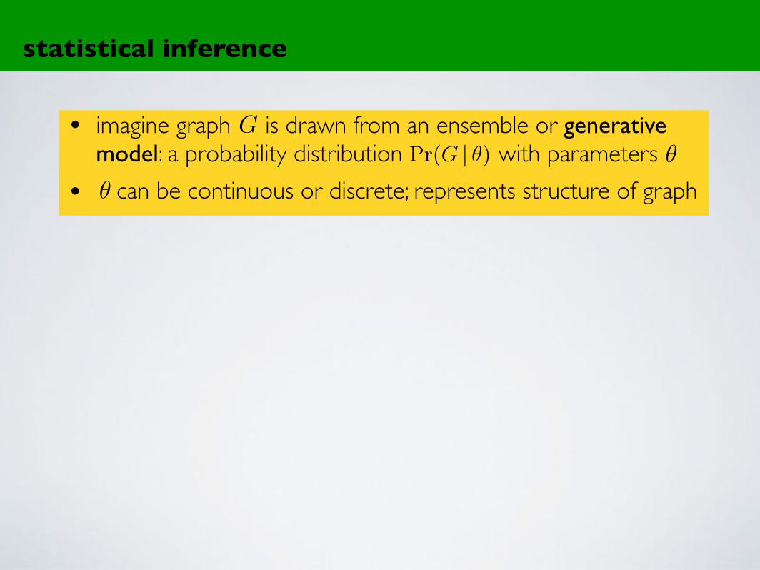
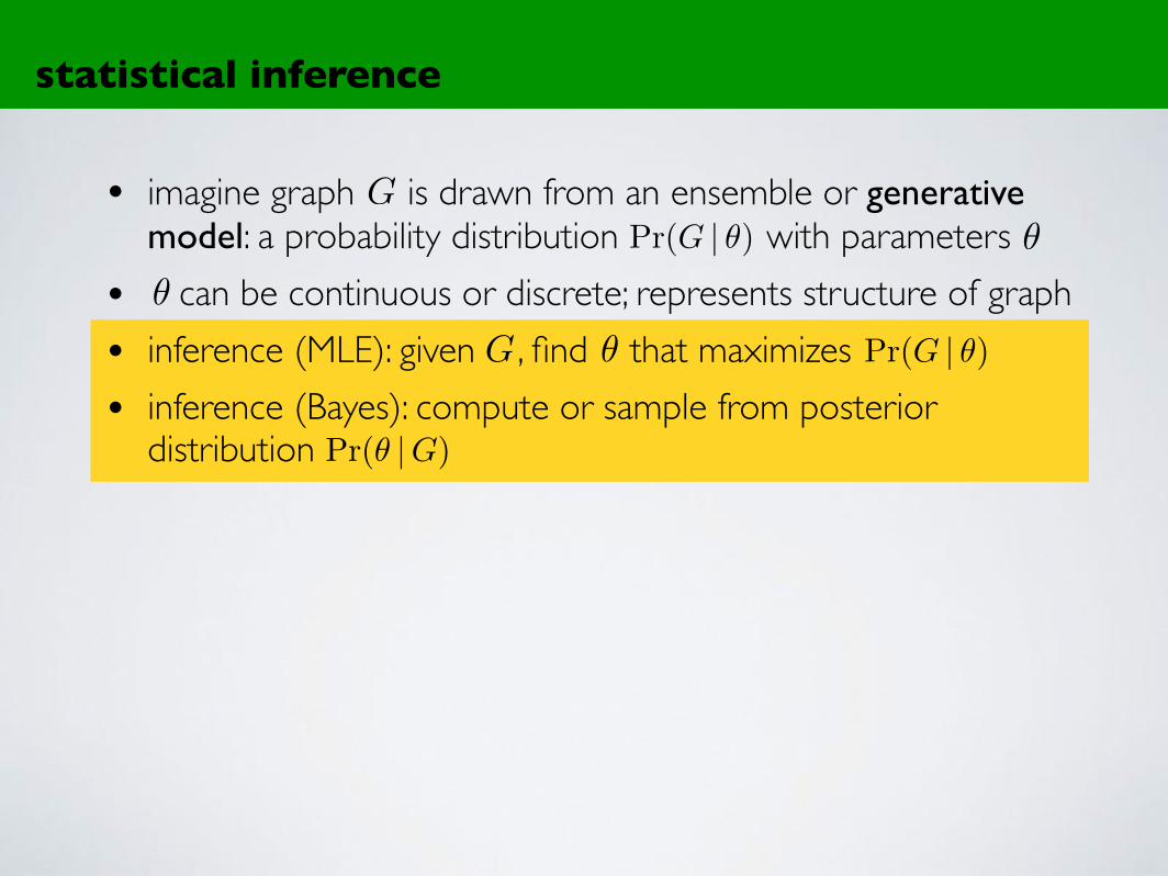
• imagine graph is drawn from an ensemble or generative model: a probability distribution with parameters
• can be continuous or discrete; represents structure of graph
statistical inference
G
✓
✓Pr(G | ✓)
• imagine graph is drawn from an ensemble or generative model: a probability distribution with parameters
• can be continuous or discrete; represents structure of graph• inference (MLE): given , find that maximizes • inference (Bayes): compute or sample from posterior
distribution
statistical inference
✓
G ✓
G✓Pr(G | ✓)
Pr(✓ |G)
Pr(G | ✓)
statistical inference
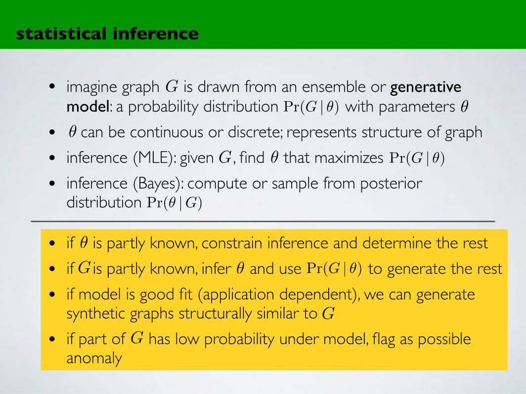
• imagine graph is drawn from an ensemble or generative model: a probability distribution with parameters
• can be continuous or discrete; represents structure of graph• inference (MLE): given , find that maximizes • inference (Bayes): compute or sample from posterior
distribution
• if is partly known, constrain inference and determine the rest• if is partly known, infer and use to generate the rest• if model is good fit (application dependent), we can generate
synthetic graphs structurally similar to • if part of has low probability under model, flag as possible
anomaly
✓
G ✓
✓
✓G
G
G
G✓Pr(G | ✓)
Pr(G | ✓)
Pr(✓ |G)
Pr(G | ✓)

statistical inference
• imagine graph is drawn from an ensemble or generative model: a probability distribution with parameters
• can be continuous or discrete; represents structure of graph• inference (MLE): given , find that maximizes • inference (Bayes): compute or sample from posterior
distribution
• if is partly known, constrain inference and determine the rest• if is partly known, infer and use to generate the rest• if model is good fit (application dependent), we can generate
synthetic graphs structurally similar to • if part of has low probability under model, flag as possible
anomaly
✓
G ✓
✓
✓G
G
G
G✓Pr(G | ✓)
Pr(G | ✓)
Pr(✓ |G)
Pr(G | ✓)
statistical inference = principled approach to
learning from data
combines tools from statistics, machine learning,
information theory, and statistical physics
quantifies uncertainty
separates the model from the learnin
g
statistical inference: key ideas
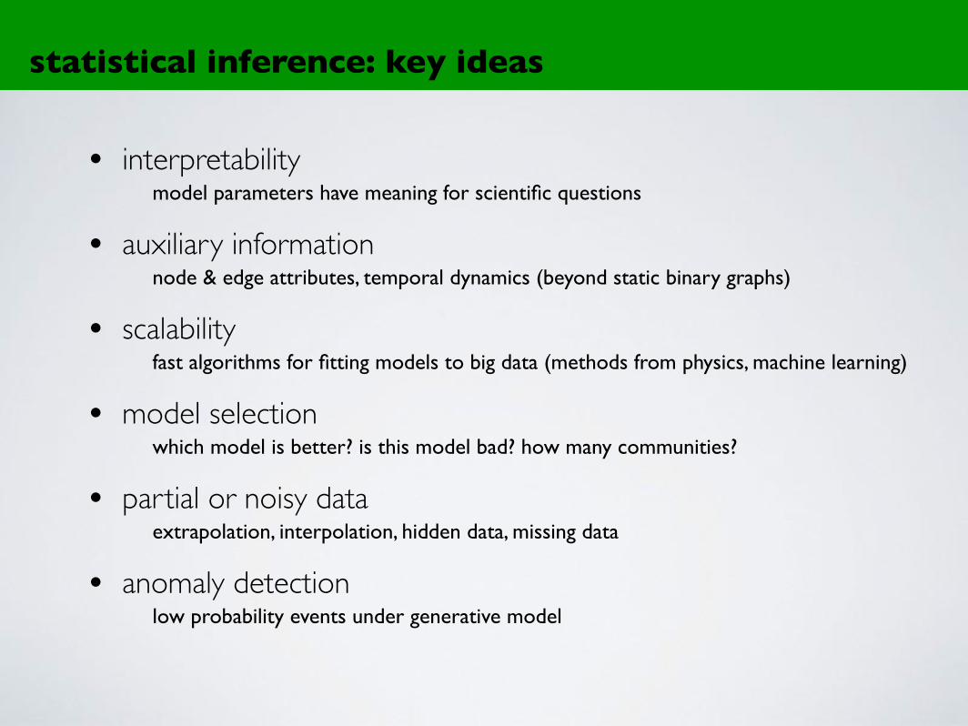
• interpretabilitymodel parameters have meaning for scientific questions
• auxiliary informationnode & edge attributes, temporal dynamics (beyond static binary graphs)
• scalabilityfast algorithms for fitting models to big data (methods from physics, machine learning)
• model selectionwhich model is better? is this model bad? how many communities?
• partial or noisy dataextrapolation, interpolation, hidden data, missing data
• anomaly detectionlow probability events under generative model
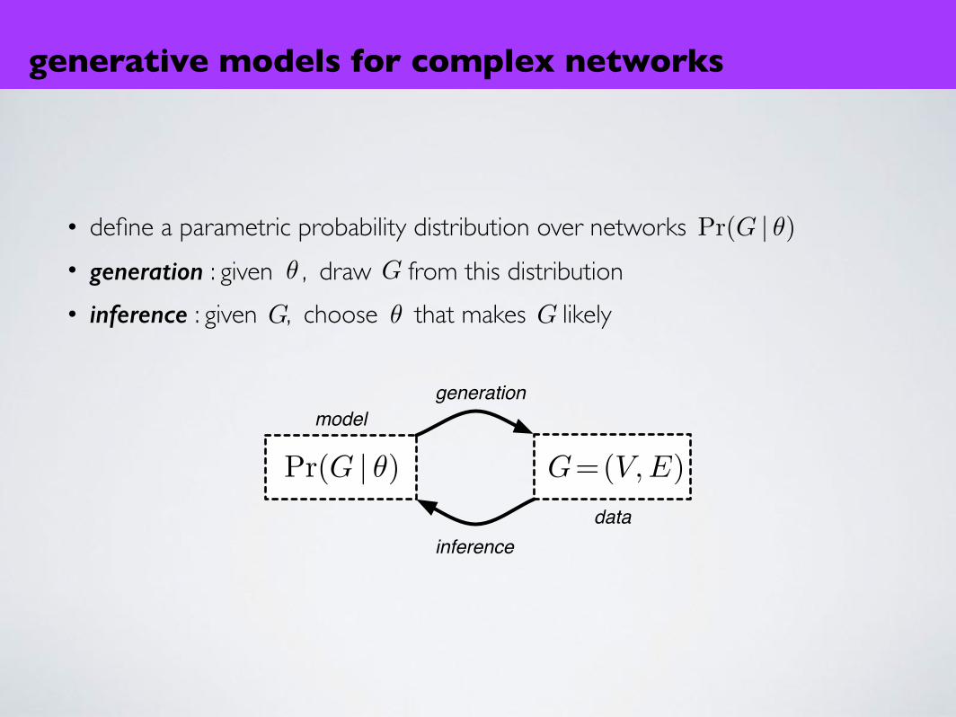
• define a parametric probability distribution over networks• generation : given , draw from this distribution• inference : given , choose that makes likely
generation
inference
model
G=(V,E)
data
Pr(G | θ)
Pr(G | ✓)✓ G
G ✓ G
generative models for complex networks

assumptions about “structure” go into
consistency
requires that edges be conditionally independent [Shalizi, Rinaldo 2011]
two general classes of these models
generative models for complex networks
general form
limn!1
Pr⇣✓ 6= ✓
⌘= 0
edge generation function
generation
inference
model
G=(V,E)
data
Pr(G | θ)
Pr(Aij | ✓)
Pr(G | ✓) =Y
ij
Pr(Aij | ✓)
generative models for complex networks
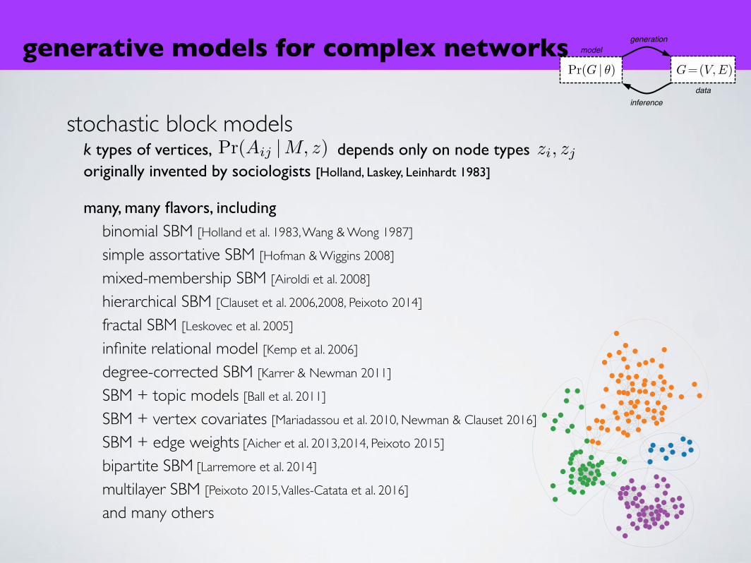
stochastic block modelsk types of vertices, depends only on node types originally invented by sociologists [Holland, Laskey, Leinhardt 1983]
many, many flavors, includingbinomial SBM [Holland et al. 1983, Wang & Wong 1987]
simple assortative SBM [Hofman & Wiggins 2008]
mixed-membership SBM [Airoldi et al. 2008]
hierarchical SBM [Clauset et al. 2006,2008, Peixoto 2014]
fractal SBM [Leskovec et al. 2005]
infinite relational model [Kemp et al. 2006]
degree-corrected SBM [Karrer & Newman 2011]
SBM + topic models [Ball et al. 2011]
SBM + vertex covariates [Mariadassou et al. 2010, Newman & Clauset 2016]
SBM + edge weights [Aicher et al. 2013,2014, Peixoto 2015]
bipartite SBM [Larremore et al. 2014]
multilayer SBM [Peixoto 2015, Valles-Catata et al. 2016]
and many others
generation
inference
model
G=(V,E)
data
Pr(G | θ)
Pr(Aij |M, z) zi, zj
00.5 1
a(t)0 10 10200
400600
0 1
alignment position t
1
23
4
56
78
9
calculate alignment scores
convert to alignment indicators
remove short aligned regions
extract highly variable regions
NGDYKEKVSNNLRAIFNKIYENLNDPKLKKHYQKDAPNYNGDYKKKVSNNLKTIFKKIYDALKDTVKETYKDDPNYNGDYKEKVSNNLRAIFKKIYDALEDTVKETYKDDPNY
166
13
16613
AB
CD

generative models for complex networks
latent space modelsnodes live in a latent space, depends only on vertex-vertex proximityoriginally invented by statisticians [Hoff, Raftery, Handcock 2002]
many, many flavors, includinglogistic function on vertex features [Hoff et al. 2002]social status / ranking [Ball, Newman 2013]nonparametric metadata relations [Kim et al. 2012]multiplicative attribute graphs [Kim & Leskovec 2010]nonparametric latent feature model [Miller et al. 2009]infinite multiple memberships [Morup et al. 2011]ecological niche model [Williams et al. 2010]hyperbolic latent spaces [Boguna et al. 2010]and many others
1094 Journal of the American Statistical Association, December 2002
Figure 1. Maximum Likelihood Estimates (a) and Bayesian Marginal
Posterior Distributions (b) for Monk Positions. The direction of a relation
is indicated by an arrow.
distances between nodes, but quite slowly in Å, as shown inFigure 2(b). Output from the chain was saved every 2,000scans, and positions of the different monks are plotted for eachsaved scan in Figure 1(b) (the plotting color for each monkis based on their mean angle from the positive x-axis andtheir mean distance from the origin). The categorization of themonks given at the beginning of this section is validated by thedistance model étting, as there is little between-group overlapin the posterior distribution of monk positions. Additionally,this model is able to quantify the extent to which some actors(such as monk 15) lie between other groups of actors.
The extent to which model ét can be improved by increas-ing the dimension of the latent space was examined by éttingthe distance model in <3, that is, z
i
2 <3 for i
D 11 : : : 1 n. Themaximum likelihood for this model is ƒ34004 in 50 param-eters, a substantial improvement over the ét in <2 at a costof 16 additional parameters. It is interesting to note that theét cannot be improved by going into higher dimensions. Thiscan be seen as follows. For a given dataset Y , the best-éttingsymmetric model (p
i1 j
Dp
j1 i
) has the property that p
i1 j
D 1for y
i1 j
Dy
j1 i
D 1, p
i1 j
D 0 for y
i1 j
Dy
j1 i
D 0, and p
i1 j
D 1=2for y
i1 j
6Dy
j1 i
. The log-likelihood of such a ét is thus ƒa log4,
where a is the number of asymmetric dyads. For the monk
0 200 600 1000
11
01
00
90
80
scan�/�(�2�x�10
3
)
lo
g�like
lih
oo
d
0 200 600 1000
46
81
01
2
scan�/�(2�x�10
3
)
alp
ha
(a) (b)
Figure 2. MCMC Diagnostics for the Monk Analysis. (a) Log-
likelihood; (b) alpha.
dataset, the number of asymmetric dyads is 26, and so themaximum possible log-likelihood under a symmetric model isƒ26 log4 D ƒ36004, which is achieved by the distance modelin <3. More precisely, there exists a set of positions O
z
i
2 <3
and a rate parameter OÅ such that lim
c
!ˆ logP4Y
—c
OÅ1 c
bZ5
Dƒ26 log4.
4.2 Florentine Families
Padgett and Ansell (1993) compiled data on marriageand business relations between 16 historically prominentFlorentine families, using a history of this period given byKent (1978). We analyze data on the marriage relations tak-ing place during the 15th century. The actors in the populationare families, and a tie is present between two families if thereis at least one marriage between them. This is an undirectedrelation, as the respective families of the husband and wife ineach marriage were not recorded. One of the 16 families hadno marriage ties to the others, and was consequently droppedfrom the analysis. If included, this family would have inénitedistance from the others in a maximum likelihood estimationand a large but énite distance in a Bayesian analysis, as deter-mined by the prior.
Modeling d
i1 j
D —z
i
ƒz
j
—1 z
i
1 z
j
2 <2 and using the param-eterization ‡
i1 j
DÅ41 ƒ
d
i1 j
5 as described in Section 2, thelikelihood of (Å1Z5 can be made arbitrarily close to 1 asÅ
! ˆ for éxed Z
D bZ; that is, the data are d2 representable.
Such a representing bZ is plotted in Figure 3(a). Family 9 is
the Medicis, whose average distance to others is greater onlythan that of families 13, the Ridolés and 16, the Tornabuonis.Another d2 representation is given in Figure 3(b). This conég-uration is similar in structure to the érst, except that the seg-ments 9-1 and 9-14-10 have been rotated. This is somewhatof an artifact of our choice of dimension: When modeled inthree dimensions, 1 and 14 are ét as being relatively equidis-tant from 6.
One drawback of the MLEs presented earlier is that theyoverét the data in a sense, as the étted probabilities of ties areall either 0 or 1 (or nearly so, for very large Å). Alternatively,a prior for Å can be formulated to keep predictive probabilitiesmore in line with our beliefs; for example, that the probabil-ity of a tie rarely goes below some small, but not inénitesi-mal value. Using the MCMC procedure outlined in Section 3,the marriage data were analyzed using an exponential priorwith mean 2 for Å and diffuse independent normal priors forthe components of Z (mean 0, standard deviation 100). TheMCMC algorithm was run for 5 Ä 106 scans, with the outputsaved every 5,000 scans. This chain mixes faster than that ofthe monk example, as can be seen in the diagnostic plots ofFigure 4 and in plots of pairwise distances between nodes (notshown). Marginal conédence regions are represented by plot-ting samples of positions from the Markov chain, shown inFigure 3(c). Note that the conédence regions include both theconégurations given in Figure 3(a) and (b). Actors 14 and 10(in red and purple) are above or below actor 1 (in green) forany particular sample; the observed overlap of these actors inthe égure is due to the bimodality of the posterior and that theplot gives the marginal posterior distributions of each actor.
generation
inference
model
G=(V,E)
data
Pr(G | θ)
Pr(Aij | f(xi, xj))

opportunities and challenges
• richly annotated dataedge weights, node attributes, time, etc.= new classes of generative models
• generalize from to ensembleuseful for modeling checking, simulating other processes, etc.
• many familiar techniquesfrequentist and Bayesian frameworksmakes probabilistic statements about observations, modelspredicting missing links leave-k-out cross validationapproximate inference techniques (EM, VB, BP, etc.)sampling techniques (MCMC, Gibbs, etc.)
• learn from partial or noisy dataextrapolation, interpolation, hidden data, missing data
n = 1
⇡
generation
inference
model
G=(V,E)
data
Pr(G | θ)
opportunities and challenges
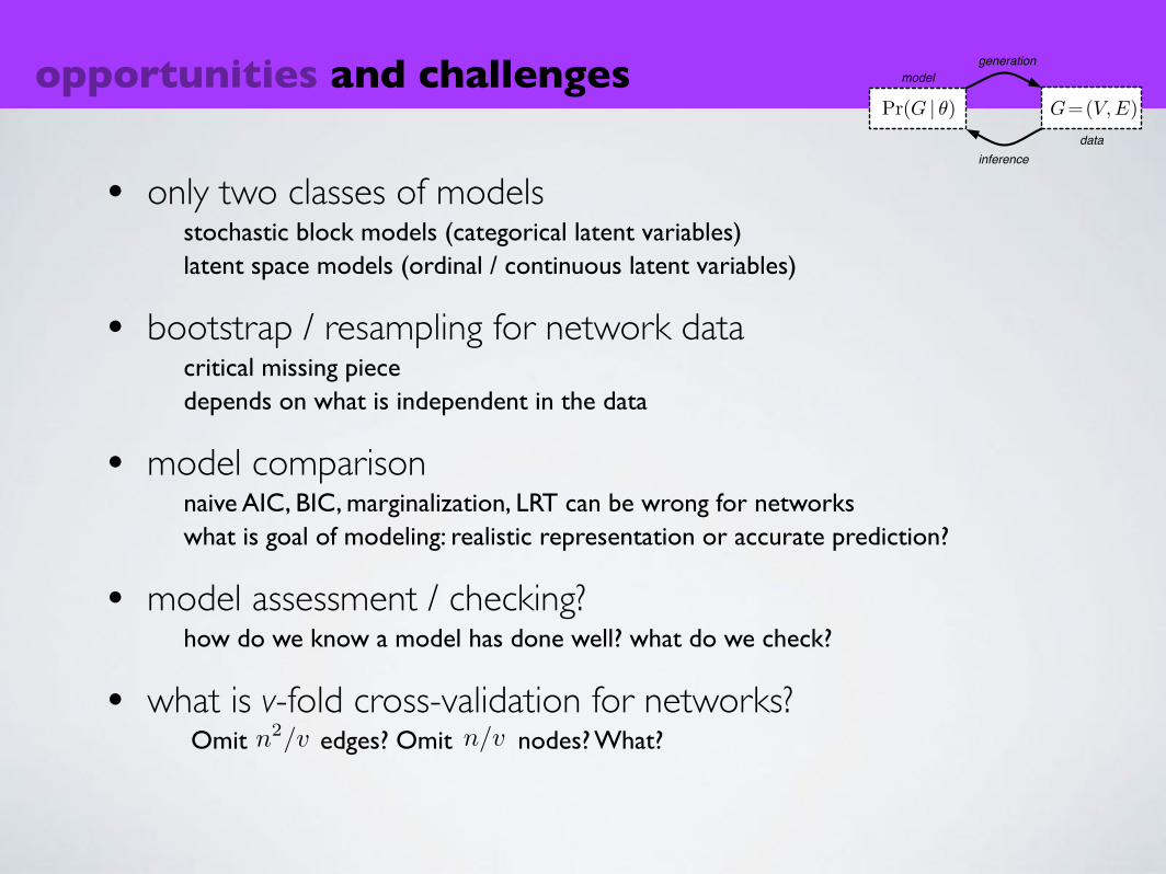
• only two classes of modelsstochastic block models (categorical latent variables)latent space models (ordinal / continuous latent variables)
• bootstrap / resampling for network datacritical missing piecedepends on what is independent in the data
• model comparisonnaive AIC, BIC, marginalization, LRT can be wrong for networkswhat is goal of modeling: realistic representation or accurate prediction?
• model assessment / checking?how do we know a model has done well? what do we check?
• what is v-fold cross-validation for networks? Omit edges? Omit nodes? What?n2/v n/v
generation
inference
model
G=(V,E)
data
Pr(G | θ)

• each vertex has type ( vertex types or groups)
• stochastic block matrix of group-level connection probabilities
• probability that are connected =
community = vertices with same pattern of inter-community connections
the stochastic block model
i zi 2 {1, . . . , k}M
k
i, j Mzi,zj
00.5
1
a(t) 0
1
0
1
020
040
060
0
0
1
alig
nmen
t pos
ition
t
1
23
4
56
78
9
calcu
late
alig
nmen
t sco
res
conv
ert t
o al
ignm
ent i
ndica
tors
rem
ove
shor
t alig
ned
regi
ons
extra
ct h
ighl
y va
riabl
e re
gion
s
NGDYKEKVSNNLRAIFNKIYENLNDPKLKKHYQKDAPNY
NGDYKKKVSNNLKTIFKKIYDALKDTVKETYKDDPNY
NGDYKEKVSNNLRAIFKKIYDALEDTVKETYKDDPNY
16
6
13
166
13
A
B
C
D
inferred M
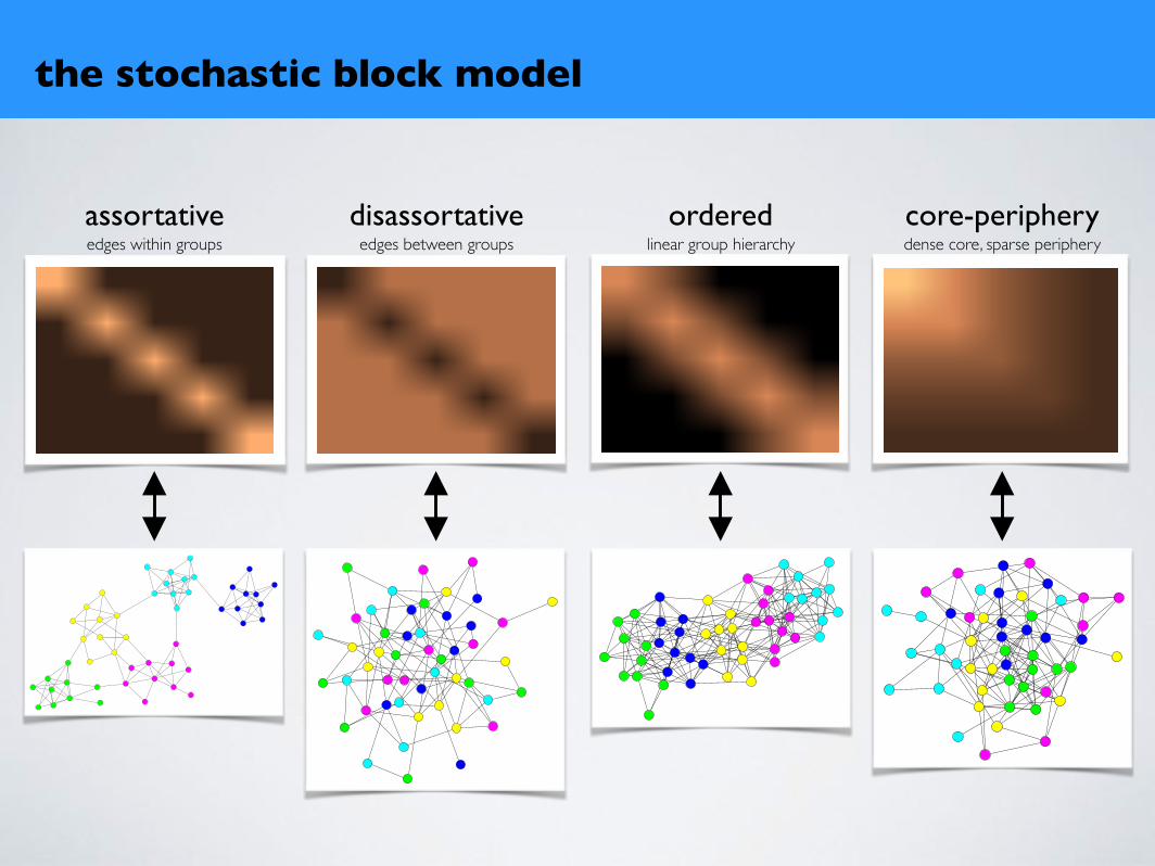
the stochastic block model
assortativeedges within groups
disassortativeedges between groups
orderedlinear group hierarchy
core-peripherydense core, sparse periphery
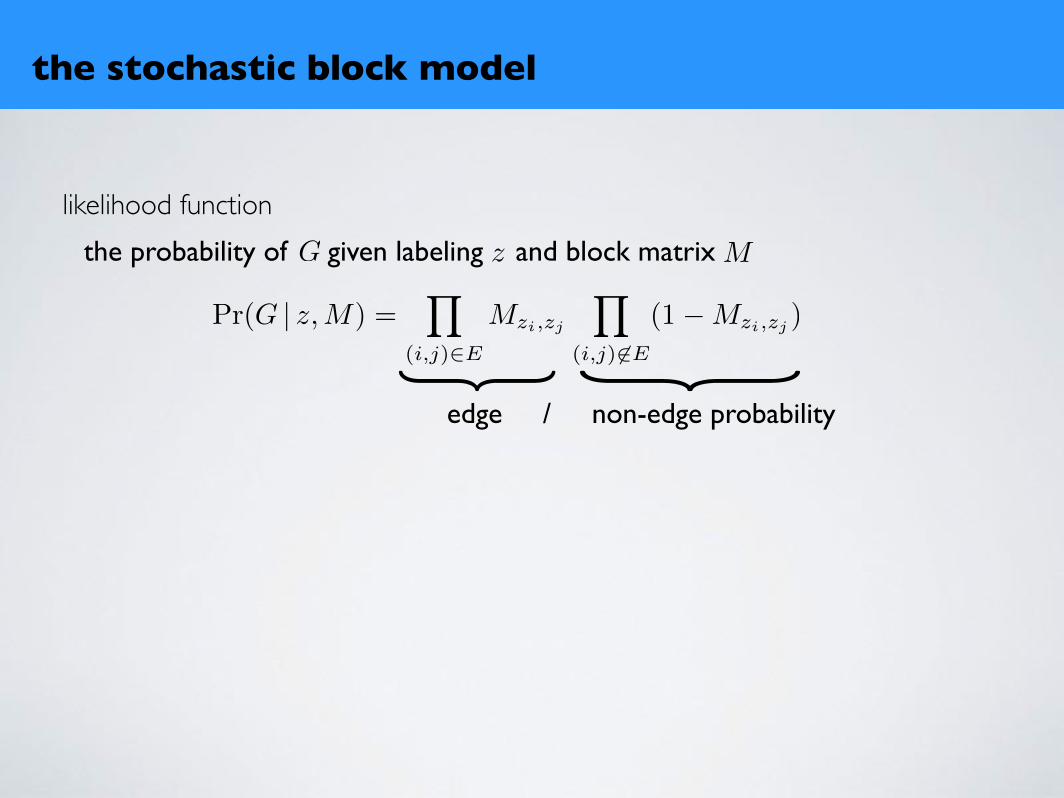
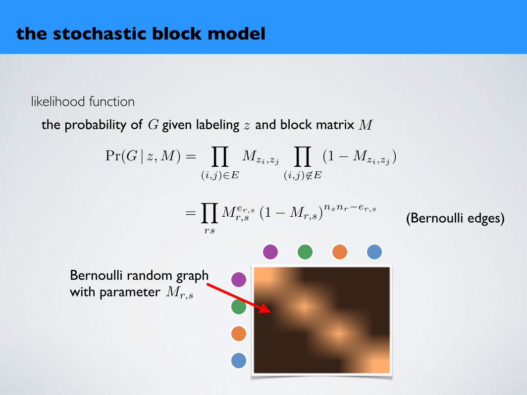
likelihood functionthe probability of given labeling and block matrix
edge / non-edge probability
} }Pr(G | z,M) =Y
(i,j)2E
Mzi,zj
Y
(i,j) 62E
(1�Mzi,zj )
the stochastic block model
zG M
likelihood functionthe probability of given labeling and block matrix
Pr(G | z,M) =Y
(i,j)2E
Mzi,zj
Y
(i,j) 62E
(1�Mzi,zj )
the stochastic block model
zG M
=Y
rs
Mer,sr,s (1�Mr,s)
nsnr�er,s(Bernoulli edges)
Bernoulli random graph with parameter Mr,s
✓a,⇤
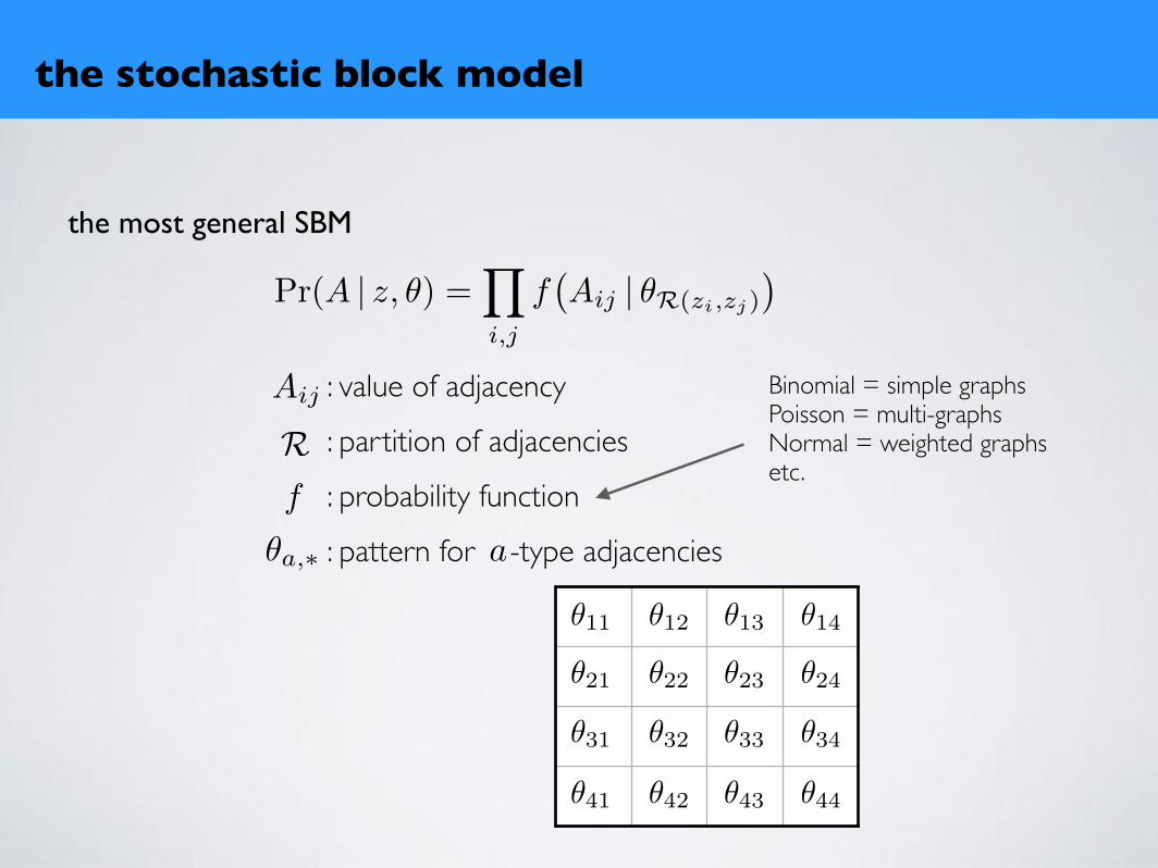
the most general SBM
the stochastic block model
Pr(A | z, ✓) =Y
i,j
f�Aij | ✓R(zi,zj)
�
f
RAij : value of adjacency
: partition of adjacencies
: probability function
: pattern for -type adjacencies
Binomial = simple graphsPoisson = multi-graphsNormal = weighted graphsetc.
a
✓11
✓22
✓33
✓44
✓12
✓21
✓31 ✓32
✓41 ✓42 ✓43
✓34
✓24
✓14✓13
✓23

degree-corrected SBM ( = Poisson)
the stochastic block model
Karrer, Newman, Phys. Rev. E (2011)
f

degree-corrected SBM ( = Poisson)
key assumptionstochastic block matrix(degree) propensity of nodelikelihood:
where
the stochastic block model
Karrer, Newman, Phys. Rev. E (2011)
f
Pr(i ! j) = ✓i✓j!zi,zj
!r,s
✓i
Pr(A | z, ✓,!) =Y
i<j
�✓i✓j!zr,zj
�Aij
Aij !exp
��✓i✓j!zr,zj
�
✓i =kiP
j kj�zi,zj!rs = mrs =
X
ij
Aij�zi,r�zj ,s
fraction of ’s group’s stubs on
} }total number of edges between andi i r s

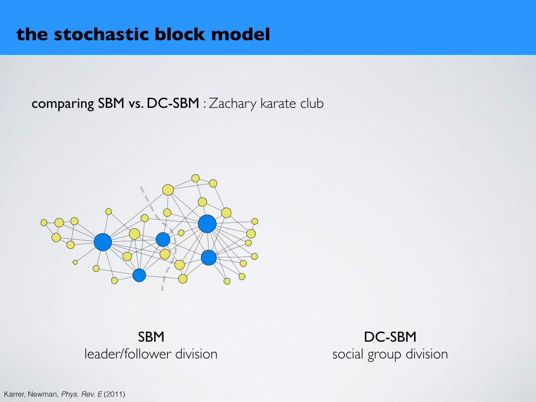
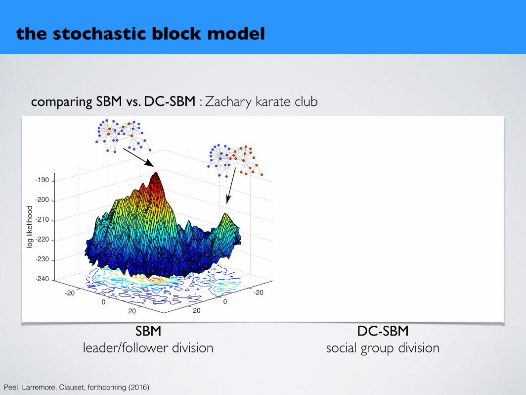
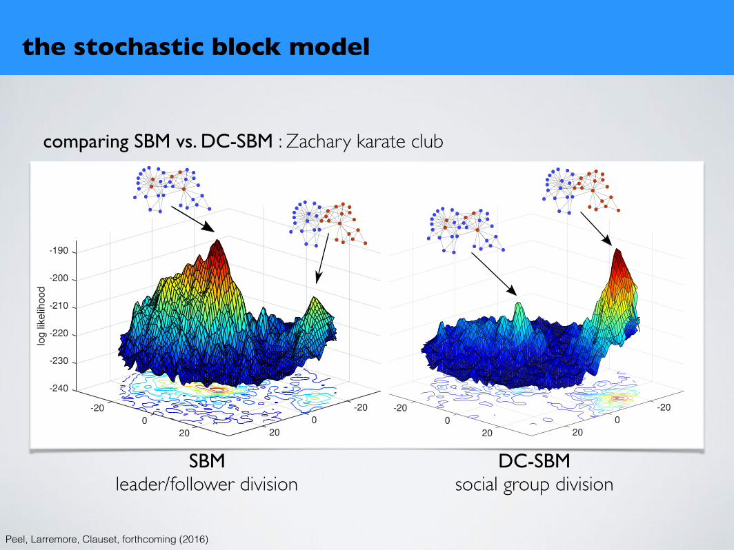
comparing SBM vs. DC-SBM : Zachary karate club
the stochastic block model
Karrer, Newman, Phys. Rev. E (2011)
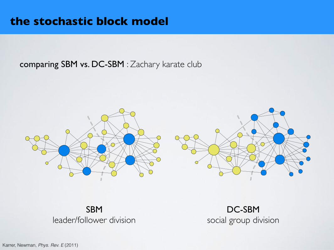
comparing SBM vs. DC-SBM : Zachary karate club
the stochastic block model
6
given i and r can thus be done in time O(K(K + ⟨k⟩)).Because these computations can be done quickly for areasonable number of communities, local vertex switch-ing algorithms, such as single-vertex Monte Carlo, can beimplemented easily. Monte Carlo, however, is slow, andwe have found competitive results using a local heuristicalgorithm similar in spirit to the Kernighan–Lin algo-rithm used in minimum-cut graph partitioning [27].Briefly, in this algorithm we divide the network into
some initial set of K communities at random. Then werepeatedly move a vertex from one group to another, se-lecting at each step the move that will most increase theobjective function—or least decrease it if no increase ispossible—subject to the restriction that each vertex maybe moved only once. When all vertices have been moved,we inspect the states through which the system passedfrom start to end of the procedure, select the one with thehighest objective score, and use this state as the startingpoint for a new iteration of the same procedure. Whena complete such iteration passes without any increase inthe objective function, the algorithm ends. As with manydeterministic algorithms, we have found it helpful to runthe calculation with several different random initial con-ditions and take the best result over all runs.
IV. RESULTS
We have tested the performance of the degree-corrected and uncorrected blockmodels in applicationsboth to real-world networks with known community as-signments and to a range of synthetic (i.e., computer-generated) networks. We evaluate performance by quan-titative comparison of the community assignments foundby the algorithms and the known assignments. As a met-ric for comparison we use the normalized mutual infor-mation, which is defined as follows [7]. Let nrs be thenumber of vertices in community r in the inferred groupassignment and in community s in the true assignment.Then define p(X = r, Y = s) = nrs/n to be the jointprobability that a randomly selected vertex is in r in theinferred assignment and s in the true assignment. Usingthis joint probability over the random variables X andY , the normalized mutual information is
NMI(X,Y ) =2MI(X,Y )
H(X) +H(Y ), (26)
where MI(X,Y ) is the mutual information and H(Z) isthe entropy of random variable Z. The normalized mu-tual information measures the similarity of the two com-munity assignments and takes a value of one if the as-signments are identical and zero if they are uncorrelated.A discussion of this and other measures can be found inRef. [28].
(a) Without degree correction
(b) With degree-correction
FIG. 1: Divisions of the karate club network found using the(a) uncorrected and (b) corrected blockmodels. The size of avertex is proportional to its degree and vertex color reflectsinferred group membership. The dashed line indicates thesplit observed in real life.
A. Empirical networks
We have tested our algorithms on real-world networksranging in size from tens to tens of thousands of ver-tices. In networks with highly homogeneous degree distri-butions we find little difference in performance betweenthe degree-corrected and uncorrected blockmodels, whichis expected since for networks with uniform degrees thetwo models have the same likelihood up to an additiveconstant. Our primary concern, therefore, is with net-works that have heterogeneous degree distributions, andwe here give two examples that show the effects of het-erogeneity clearly.The first example, widely studied in the field, is the
“karate club” network of Zachary [29]. This is a socialnetwork representing friendship patterns between the 34members of a karate club at a US university. The clubin question is known to have split into two different fac-tions as a result of an internal dispute, and the membersof each faction are known. It has been demonstratedthat the factions can be extracted from a knowledgeof the complete network by many community detectionmethods.Applying our inference algorithms to this network, us-
SBMleader/follower division
DC-SBMsocial group division
Karrer, Newman, Phys. Rev. E (2011)
comparing SBM vs. DC-SBM : Zachary karate club
the stochastic block model
6
given i and r can thus be done in time O(K(K + ⟨k⟩)).Because these computations can be done quickly for areasonable number of communities, local vertex switch-ing algorithms, such as single-vertex Monte Carlo, can beimplemented easily. Monte Carlo, however, is slow, andwe have found competitive results using a local heuristicalgorithm similar in spirit to the Kernighan–Lin algo-rithm used in minimum-cut graph partitioning [27].Briefly, in this algorithm we divide the network into
some initial set of K communities at random. Then werepeatedly move a vertex from one group to another, se-lecting at each step the move that will most increase theobjective function—or least decrease it if no increase ispossible—subject to the restriction that each vertex maybe moved only once. When all vertices have been moved,we inspect the states through which the system passedfrom start to end of the procedure, select the one with thehighest objective score, and use this state as the startingpoint for a new iteration of the same procedure. Whena complete such iteration passes without any increase inthe objective function, the algorithm ends. As with manydeterministic algorithms, we have found it helpful to runthe calculation with several different random initial con-ditions and take the best result over all runs.
IV. RESULTS
We have tested the performance of the degree-corrected and uncorrected blockmodels in applicationsboth to real-world networks with known community as-signments and to a range of synthetic (i.e., computer-generated) networks. We evaluate performance by quan-titative comparison of the community assignments foundby the algorithms and the known assignments. As a met-ric for comparison we use the normalized mutual infor-mation, which is defined as follows [7]. Let nrs be thenumber of vertices in community r in the inferred groupassignment and in community s in the true assignment.Then define p(X = r, Y = s) = nrs/n to be the jointprobability that a randomly selected vertex is in r in theinferred assignment and s in the true assignment. Usingthis joint probability over the random variables X andY , the normalized mutual information is
NMI(X,Y ) =2MI(X,Y )
H(X) +H(Y ), (26)
where MI(X,Y ) is the mutual information and H(Z) isthe entropy of random variable Z. The normalized mu-tual information measures the similarity of the two com-munity assignments and takes a value of one if the as-signments are identical and zero if they are uncorrelated.A discussion of this and other measures can be found inRef. [28].
(a) Without degree correction
(b) With degree-correction
FIG. 1: Divisions of the karate club network found using the(a) uncorrected and (b) corrected blockmodels. The size of avertex is proportional to its degree and vertex color reflectsinferred group membership. The dashed line indicates thesplit observed in real life.
A. Empirical networks
We have tested our algorithms on real-world networksranging in size from tens to tens of thousands of ver-tices. In networks with highly homogeneous degree distri-butions we find little difference in performance betweenthe degree-corrected and uncorrected blockmodels, whichis expected since for networks with uniform degrees thetwo models have the same likelihood up to an additiveconstant. Our primary concern, therefore, is with net-works that have heterogeneous degree distributions, andwe here give two examples that show the effects of het-erogeneity clearly.The first example, widely studied in the field, is the
“karate club” network of Zachary [29]. This is a socialnetwork representing friendship patterns between the 34members of a karate club at a US university. The clubin question is known to have split into two different fac-tions as a result of an internal dispute, and the membersof each faction are known. It has been demonstratedthat the factions can be extracted from a knowledgeof the complete network by many community detectionmethods.Applying our inference algorithms to this network, us-
SBMleader/follower division
DC-SBMsocial group division
Karrer, Newman, Phys. Rev. E (2011)
comparing SBM vs. DC-SBM : Zachary karate club
the stochastic block model
Peel, Larremore, Clauset, forthcoming (2016)
SBMleader/follower division
DC-SBMsocial group division
-400
-395
-390
-20
-385
-20
log likeliho
od
-380
-375
0
0
20
20
-240
-230
-220
-20
-20
-210
log likeliho
od
-200
-190
0
0
20
20
-400
-395
-390
-20
-385
-20
log likeliho
od
-380
-375
0
0
20
20
-240
-230
-220
-20
-20
-210
log likeliho
od
-200
-190
0
0
20
20

extending the SBM
many variants! we’ll cover three:
• bipartite community structure
• weighted community structure
• hierarchical community structure
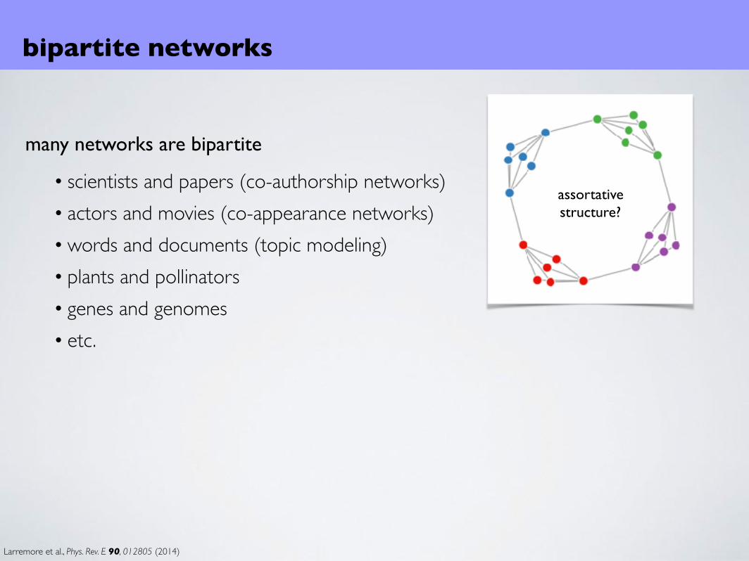
bipartite networks
many networks are bipartite
• scientists and papers (co-authorship networks)• actors and movies (co-appearance networks)• words and documents (topic modeling)• plants and pollinators• genes and genomes• etc.
assortativestructure?
Larremore et al., Phys. Rev. E 90, 012805 (2014)
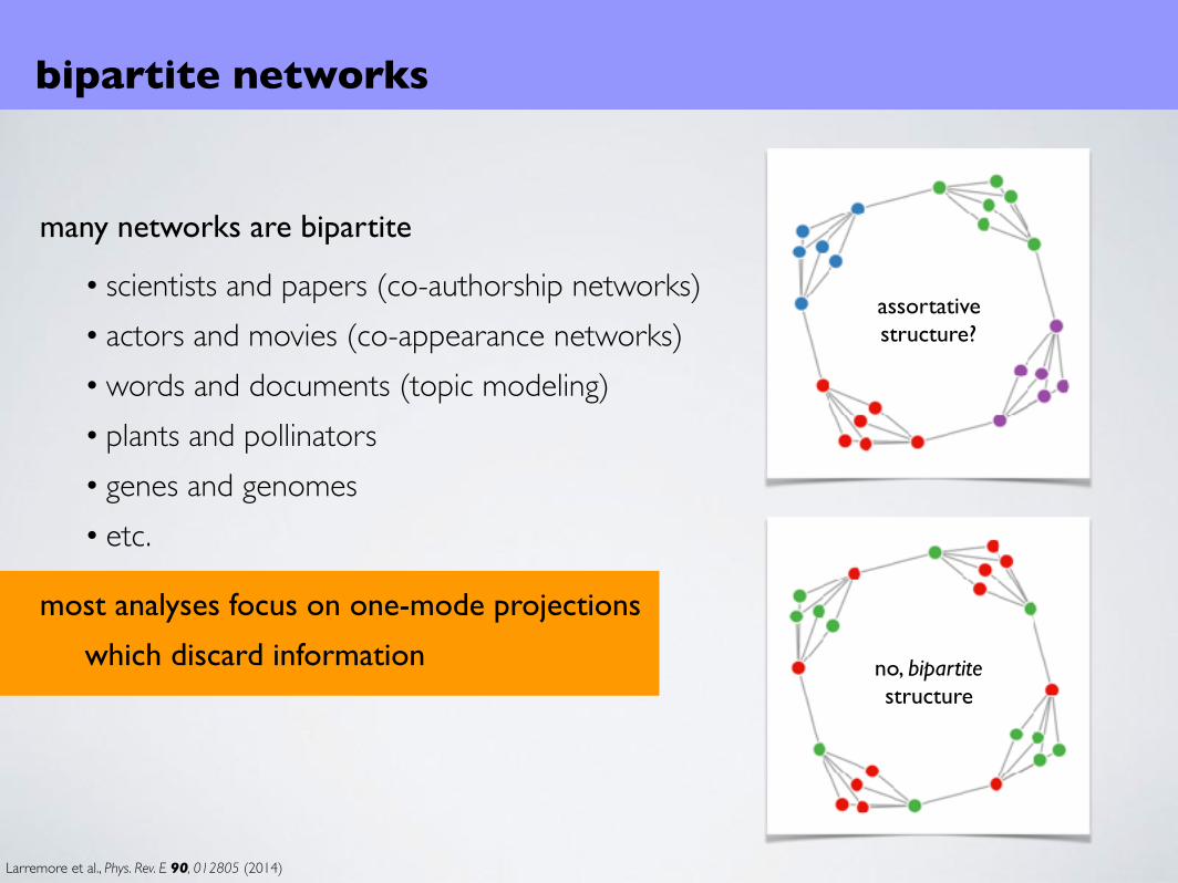
bipartite networks
many networks are bipartite
• scientists and papers (co-authorship networks)• actors and movies (co-appearance networks)• words and documents (topic modeling)• plants and pollinators• genes and genomes• etc.
most analyses focus on one-mode projections
which discard information
assortativestructure?
no, bipartitestructure
Larremore et al., Phys. Rev. E 90, 012805 (2014)
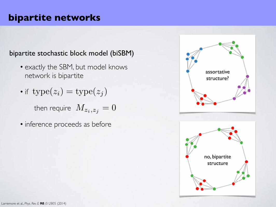
bipartite networks
bipartite stochastic block model (biSBM)
• exactly the SBM, but model knows network is bipartite
• if
then require
• inference proceeds as before
assortativestructure?
no, bipartitestructure
Mzi,zj = 0
type(zi) = type(zj)
Larremore et al., Phys. Rev. E 90, 012805 (2014)
degr
ee−c
orre
cted
bSB
M li
kelih
ood
scor
e, E
q. (1
6)
−890
−880
−870
−860
−850
−840
SBM K=4biSBM K ,K = 3,2a b
SBM K=5biSBM K ,K = 3,2a b
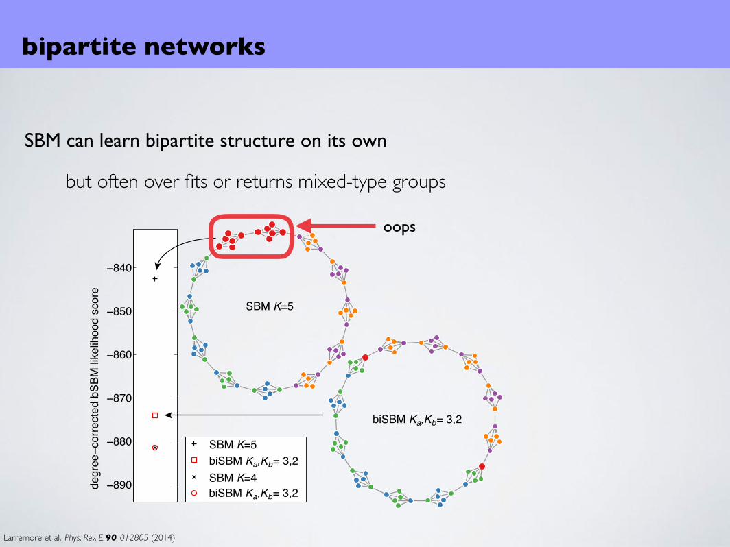
SBM K=5
biSBM K ,K = 3,2a b
SBM can learn bipartite structure on its own
but often over fits or returns mixed-type groups
bipartite networks
Larremore et al., Phys. Rev. E 90, 012805 (2014)
oops
bipartite stochastic block model (biSBM)
• how do we know it works well?
bipartite networks
Larremore et al., Phys. Rev. E 90, 012805 (2014)

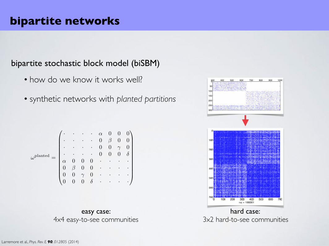
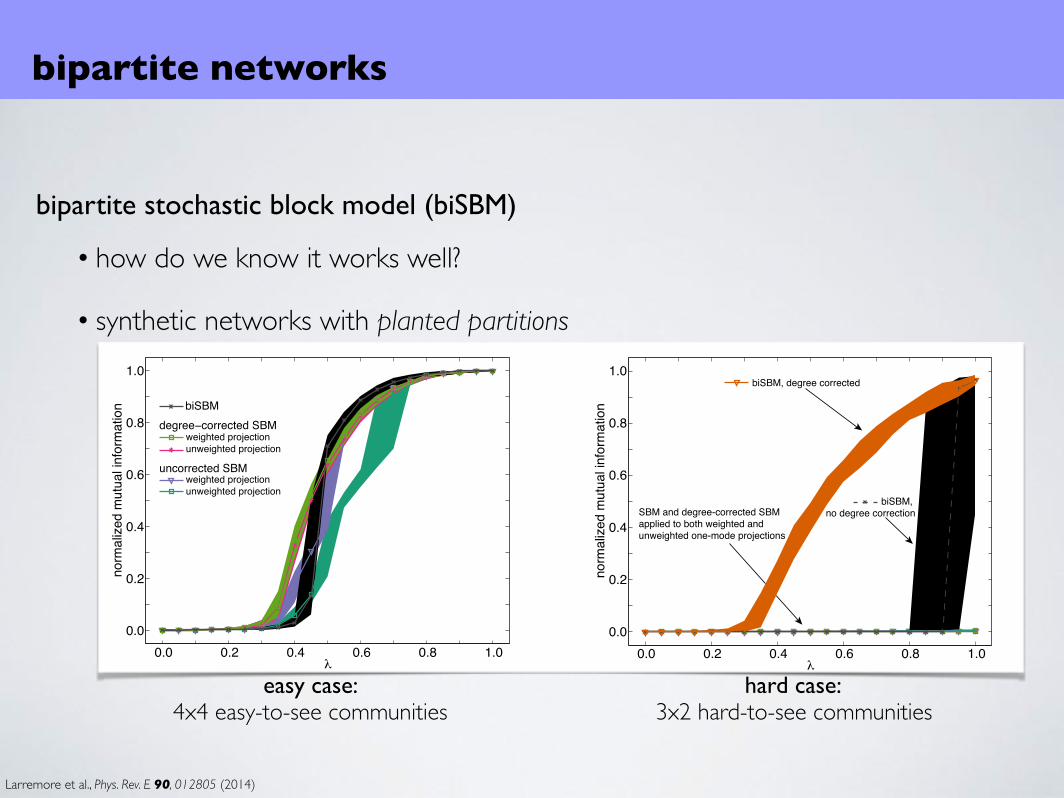
bipartite stochastic block model (biSBM)
• how do we know it works well?
• synthetic networks with planted partitions
bipartite networks
Larremore et al., Phys. Rev. E 90, 012805 (2014)
!planted =
0
BBBBBBBBBB@
· · · · ↵ 0 0 0· · · · 0 � 0 0· · · · 0 0 � 0· · · · 0 0 0 �↵ 0 0 0 · · · ·0 � 0 0 · · · ·0 0 � 0 · · · ·0 0 0 � · · · ·
1
CCCCCCCCCCA
!planted =
0
BBBB@
· · · ✏ 0· · · 0 ✏· · · � �✏ 0 � · ·0 ✏ � · ·
1
CCCCA
easy case:4x4 easy-to-see communities
hard case:3x2 hard-to-see communities
bipartite stochastic block model (biSBM)
• how do we know it works well?
• synthetic networks with planted partitions
bipartite networks
Larremore et al., Phys. Rev. E 90, 012805 (2014)
300 400 500 600 700 800 900 10000
50
100
150
200
250
300
easy case:4x4 easy-to-see communities
hard case:3x2 hard-to-see communities
!planted =
0
BBBBBBBBBB@
· · · · ↵ 0 0 0· · · · 0 � 0 0· · · · 0 0 � 0· · · · 0 0 0 �↵ 0 0 0 · · · ·0 � 0 0 · · · ·0 0 � 0 · · · ·0 0 0 � · · · ·
1
CCCCCCCCCCA
bipartite stochastic block model (biSBM)
• how do we know it works well?
• synthetic networks with planted partitions
bipartite networks
Larremore et al., Phys. Rev. E 90, 012805 (2014)
0.0 0.2 0.4 0.6 0.8 1.00.0
0.2
0.4
0.6
0.8
1.0
λ
norm
aliz
ed m
utua
l inf
orm
atio
n
weighted projectionunweighted projection
weighted projectionunweighted projection
degree−corrected SBM
uncorrected SBM
biSBM
A
SBM and degree-corrected SBMapplied to both weighted and unweighted one-mode projections
0.0 0.2 0.4 0.6 0.8 1.00.0
0.2
0.4
0.6
0.8
1.0
λ
norm
aliz
ed m
utua
l inf
orm
atio
n
biSBM, degree corrected
biSBM, no degree correction
B
easy case:4x4 easy-to-see communities
hard case:3x2 hard-to-see communities
bipartite networks
bipartite stochastic block model (biSBM)
• always find pure-type communities
• more accurate than modeling one-mode projections (even weighted projections)
• finds communities in both modes
Larremore et al., Phys. Rev. E 90, 012805 (2014)
bipartite networks
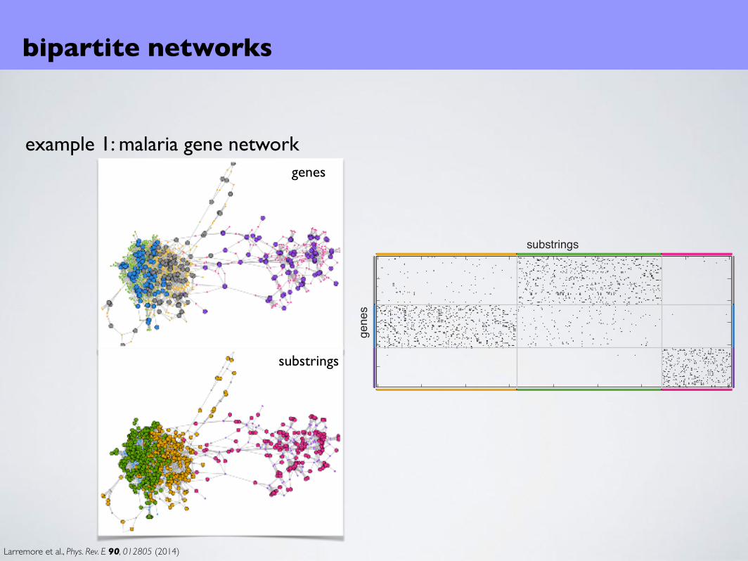
example 1: malaria gene network
substrings
genes
Larremore et al., Phys. Rev. E 90, 012805 (2014)
genes
substrings
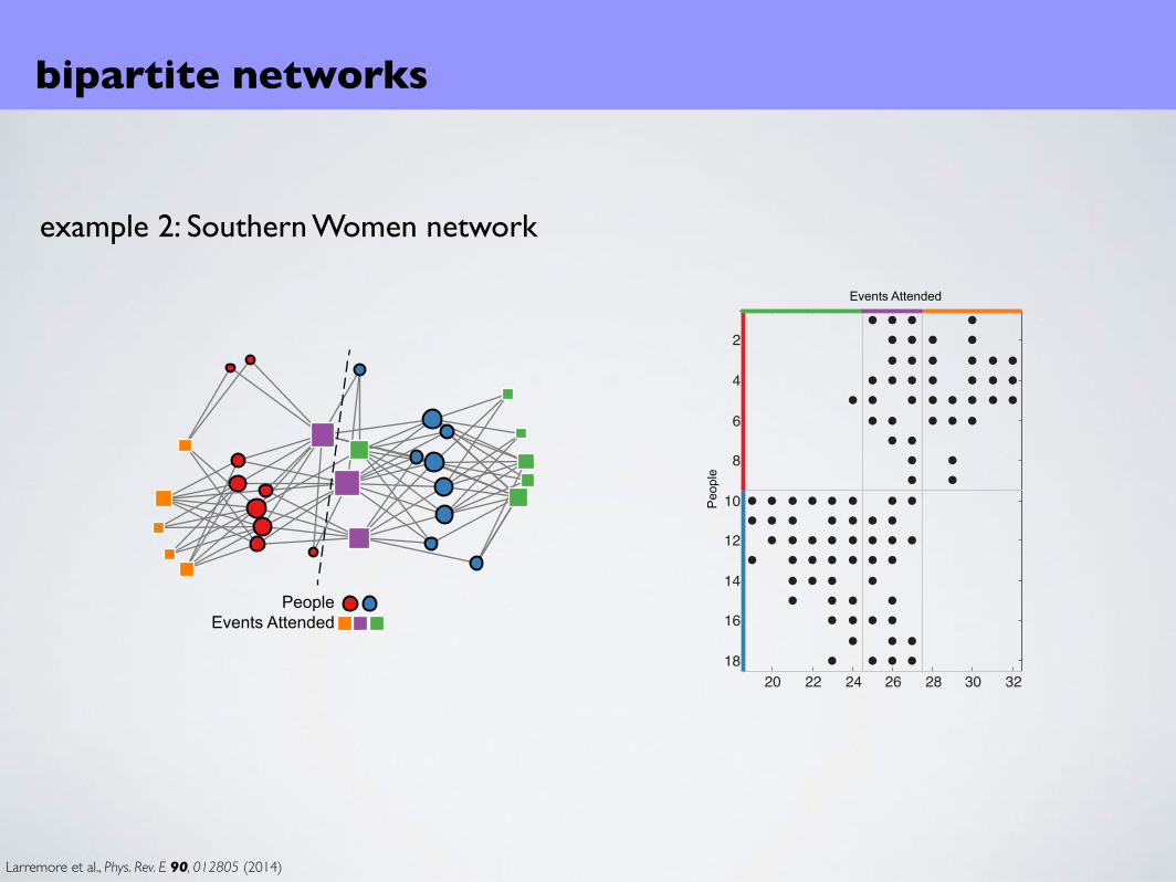
example 2: Southern Women network
PeopleEvents Attended
20 22 24 26 28 30 32
2
4
6
8
10
12
14
16
18
Peo
ple
Events Attended
bipartite networks
Larremore et al., Phys. Rev. E 90, 012805 (2014)
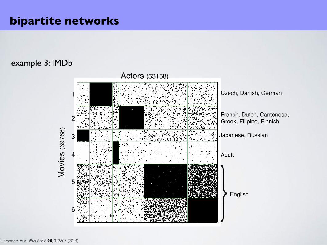
example 3: IMDb
bipartite networks
Larremore et al., Phys. Rev. E 90, 012805 (2014)
Actors (53158)
Mov
ies
(397
68)
1
2
3
4
5
6 } English
Japanese, Russian
French, Dutch, Cantonese, Greek, Filipino, Finnish
Czech, Danish, German
Adult

bipartite networks
Peixoto, Phys. Rev. Lett. 110, 148701 (2013)Guimera et al., PLOS ONE 7(9), e44620 (2012)
Parsimonious Module Inference in Large Networks
Tiago P. Peixoto*
Institut fur Theoretische Physik, Universitat Bremen, Hochschulring 18, D-28359 Bremen, Germany(Received 19 December 2012; published 5 April 2013; publisher error corrected 5 April 2013)
We investigate the detectability of modules in large networks when the number of modules is not known
in advance. We employ the minimum description length principle which seeks to minimize the total
amount of information required to describe the network, and avoid overfitting. According to this criterion,
we obtain general bounds on the detectability of any prescribed block structure, given the number of nodes
and edges in the sampled network. We also obtain that the maximum number of detectable blocks scales
asffiffiffiffiN
p, where N is the number of nodes in the network, for a fixed average degree hki. We also show that
the simplicity of the minimum description length approach yields an efficient multilevel Monte Carlo
inference algorithm with a complexity of Oð!N logNÞ, if the number of blocks is unknown, and Oð!NÞ ifit is known, where ! is the mixing time of the Markov chain. We illustrate the application of the method on
a large network of actors and films with over 106 edges, and a dissortative, bipartite block structure.
DOI: 10.1103/PhysRevLett.110.148701 PACS numbers: 89.75.Hc, 02.50.Tt, 89.70.Cf
The detection of modules—or communities—is one ofthe most intensely studied problems in the recent literatureof network systems [1,2]. The use of generative modelsfor this purpose, such as the stochastic blockmodel family[3–20], has been gaining increasing attention. Thisapproach contrasts drastically with the majority of othermethods thus far employed in the field (such as modularitymaximization [21]), since not only is it derived from firstprinciples, but also it is not restricted to purely assortativeand undirected community structures. However, mostinference methods used to obtain the most likely block-model assume that the number of communities is known inadvance [14,18,22–25]. Unfortunately, in most practicalcases this quantity is completely unknown, and one wouldlike to infer it from the data as well. Here we explore a veryefficient way of obtaining this information from the data,known as the minimum description length principle(MDL) [26,27], which predicates that the best choice ofmodel which fits given data is the one which most com-presses it, i.e., minimizes the total amount of informationrequired to describe it. This approach has been introducedin the task of blockmodel inference in Ref. [28]. Here, wegeneralize it to accommodate an arbitrarily large numberof communities, and to obtain general bounds on thedetectability of arbitrary community structures. We alsoshow that, according to this criterion, the maximum num-ber of detectable blocks scales as
ffiffiffiffiN
p, where N is the
number of nodes in the network. Since the MDL approachresults in a simple penalty on the log-likelihood, we use itto implement an efficient multilevel Monte Carlo algo-rithm with an overall complexity of Oð!N logNÞ, where! is the average mixing time of the Markov chain, whichcan be used to infer arbitrary block structures on very largenetworks.
The model.—The stochastic blockmodel ensemble iscomposed of graphs with N nodes, each belonging to one
of B blocks, and the number of edges between nodes ofblocks r and s is given by the matrix ers (or twice thatnumber if r ¼ s). The degree-corrected variant [14] furtherimposes that each node i has a degree given by ki, wherethe set fkig is an additional parameter set of the model. Thedirected version of both models is analogously defined,with ers becoming asymmetric, and fk$i g together withfkþi g fixing the in- and out-degrees of the nodes, respec-tively. These ensembles are characterized by their micro-canonical entropy S ¼ ln!, where ! is the total numberof network realizations [29]. The entropy can be computedanalytically in both cases [30],
St ffi E$ 1
2
X
rs
ers ln"ersnrns
#; (1)
for the traditional blockmodel ensemble and,
Sc ffi $E$X
k
Nk lnk!$1
2
X
rs
ers ln"erseres
#; (2)
for the degree corrected variant, where in both cases E ¼Prsers=2 is the total number of edges, nr is the number of
nodes which belong to block r, and Nk is the total numberof nodes with degree k, and er ¼
Psers is the number
of half-edges incident on block r. The directed caseis analogous [30] (see Supplemental Material [31] for anoverview).The detection problem consists in obtaining the block
partition fbig which is the most likely, when given anunlabeled network G, where bi is the block label ofnode i. This is done by maximizing the log-likelihoodlnP that the network G is observed, given the modelcompatible with a chosen block partition. Since we havesimply P ¼ 1=!, maximizing lnP is equivalent to mini-mize the entropy St=c, which is the language we will usehenceforth. Entropy minimization is well defined, but only
PRL 110, 148701 (2013) P HY S I CA L R EV I EW LE T T E R Sweek ending5 APRIL 2013
0031-9007=13=110(14)=148701(5) 148701-1 ! 2013 American Physical Society
other approaches
minimum description length (MDL) principlelearns that a network is bipartite
marginalize over bipartite SBM parameterizations
Predicting Human Preferences Using the Block Structureof Complex Social NetworksRoger Guimera1,2*, Alejandro Llorente3, Esteban Moro4,5,3, Marta Sales-Pardo2
1 Institucio Catalana de Recerca i Estudis Avancats, Barcelona, Catalonia, Spain, 2 Departament d’Enginyeria Qumica, Universitat Rovira i Virgili, Tarragona, Catalonia,
Spain, 3 Instituto de Ingenierıa del Conocimiento, Universidad Autonoma de Madrid, Madrid, Spain, 4 Departamento de Matematicas & Grupo Interdisciplinar de Sistemas
Complejos, Universidad Carlos III de Madrid, Leganes, Madrid, Spain, 5 Instituto de Ciencias Matematicas, Consejo Superior de Investigaciones Cientıficas-Autonomous
University of Madrid-Universidad Complutense de Madrid-Universidad Carlos III de Madrid, Madrid, Madrid, Spain
Abstract
With ever-increasing available data, predicting individuals’ preferences and helping them locate the most relevantinformation has become a pressing need. Understanding and predicting preferences is also important from a fundamentalpoint of view, as part of what has been called a ‘‘new’’ computational social science. Here, we propose a novel approachbased on stochastic block models, which have been developed by sociologists as plausible models of complex networks ofsocial interactions. Our model is in the spirit of predicting individuals’ preferences based on the preferences of others but,rather than fitting a particular model, we rely on a Bayesian approach that samples over the ensemble of all possiblemodels. We show that our approach is considerably more accurate than leading recommender algorithms, with majorrelative improvements between 38% and 99% over industry-level algorithms. Besides, our approach sheds light on decision-making processes by identifying groups of individuals that have consistently similar preferences, and enabling the analysisof the characteristics of those groups.
Citation: Guimera R, Llorente A, Moro E, Sales-Pardo M (2012) Predicting Human Preferences Using the Block Structure of Complex Social Networks. PLoSONE 7(9): e44620. doi:10.1371/journal.pone.0044620
Editor: Santo Fortunato, Aalto University, Finland
Received July 2, 2012; Accepted August 6, 2012; Published September 11, 2012
Copyright: ! 2012 Guimera et al. This is an open-access article distributed under the terms of the Creative Commons Attribution License, which permitsunrestricted use, distribution, and reproduction in any medium, provided the original author and source are credited.
Funding: This work was supported by a James S. McDonnell Foundation Research Award (RG and MSP), grants PIRG-GA-2010-277166 (RG) and PIRG-GA-2010-268342 (MSP) from the European Union, and grants FIS2010-18639 (RG and MSP), FIS2006-01485 (MOSAICO) (EM) and FIS2010-22047-C05-04 (EM) from theSpanish Ministerio de Economıa y Competitividad. The funders had no role in study design, data collection and analysis, decision to publish, or preparation of themanuscript.
Competing Interests: The authors have declared that no competing interests exist.
* E-mail: [email protected]
Introduction
Humans generate information at an unprecedented pace, withsome estimates suggesting that in a year we now produce on theorder of 1021 bytes of data, millions of times the amount ofinformation in all the books ever written [1]. In this context,predicting individuals’ preferences and helping them locate themost relevant information has become a pressing need. Thisexplains the outburst, during the last years, of research onrecommender systems, which aim to identify items (movies orbooks, for example) that are potentially interesting to a givenindividual [2–4].
However, understanding and ultimately predicting humanpreferences and behaviors is also important from a fundamentalpoint of view. Indeed, the digital traces that we leave with all sortsof everyday activities (shopping, communicating with others,traveling) are ushering in a new kind of computational socialscience [5,6], which aims to shed light on human mobility [7,8],activity patterns [9], decision-making processes [10], socialinfluence [11–13], and the impact of all these in collective humanbehavior [14,15].
Existing recommender systems are good at solving the practicalproblem of providing quick estimates of individuals’ preferences,but they often emphasize computational performance over otherimportant questions such as whether the algorithms are mathe-matically well-grounded or whether the implicit models and
assumptions are easy to interpret (and therefore to modify and finetune). In contrast, algorithms that are based on plausible, easily-interpretable assumptions and that are based on solid mathemat-ical grounds are useful in themselves and, arguably, hold the mostpotential to advance in the solution of the problem at thefundamental and practical levels. Here we present one suchapproach and show that it performs better than state-of-the-artrecommender systems.
In particular, we focus on what is called collaborative filtering[16], namely making predictions about preferences based onpreferences previously expressed by users. The underlyingassumption in virtually all collaborative filtering approaches isthat similar people have similar ‘‘interactions’’ with similaritems. This consideration is usually taken into accountheuristically. For example, in memory-based methods [16],one tries to identify users that are similar to the one for whichwe seek a prediction; or items that are similar to the targetitem. From these ‘‘neighbors’’ one then obtains a weightedaverage. In matrix factorization approaches [17], one assumesthat each user and item can be characterized by a low-dimensional ‘‘feature vector,’’ and that the rating of an item bya user is the product of their feature vectors.
In contrast, we base our predictions in a family of models [18–21] that have been developed and are widely used by sociologistsas plausible models of complex social networks, that is, of howsocial actors establish relationships (friendship relationships with
PLOS ONE | www.plosone.org 1 September 2012 | Volume 7 | Issue 9 | e44620
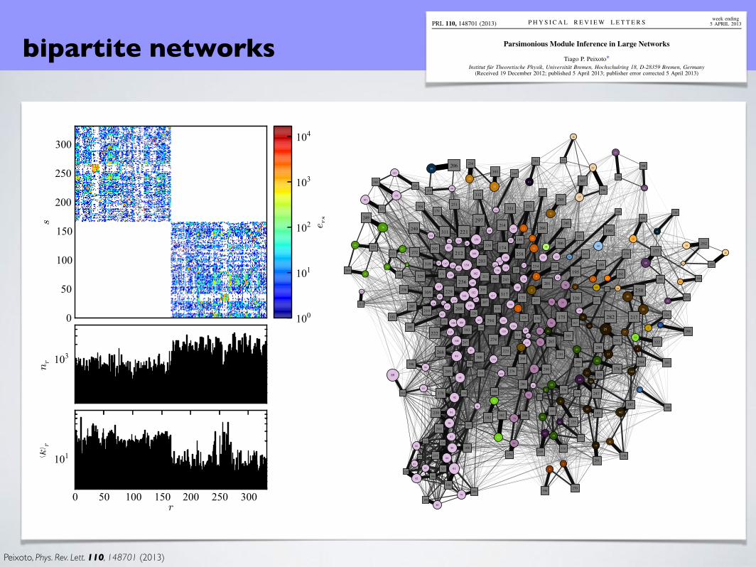
bipartite networks
Peixoto, Phys. Rev. Lett. 110, 148701 (2013)
135
223
72
317
32
253
63
182
46
302
66
232
133
246
8
178
116
320
161
175
53
292
14
216
6
278
12
213
108
301
156
195
128
233
50
222
104
211
146
256
162
166
119
239
21
206
115
190154
313
155
326
38
286
152
319
89
238
9
281
49
293
93
269
153
227
23
237
57
289
151
179
71
276
19
173
137
308
60
330
69
248
42
297
134
1722
285
109
192
139
325
27
185
5
328
67
220
129224
40
299
31
183
111
199
61
228
114
221
106
242
84
189
97
291
90
294
44
304
163
203127
324
149
268
118
234
124
201
136
288
164
212
52
17718
240
101
298
150 254
75
193
16
235
28
176
13
266
100
329
39
275
145
171
158
181
103
258
112
327
43
210
81
271
131
321
121
249
148
279
3
230
70
262
88
280
29
274
95
284
126
252
64
209
141
245
91
314
92
261
76
174
4
188
30
250
68296
123
196
82
322
74
307
17
208
110
243
24
312
34
323
132
244
47
306
41
167
87
194
125272
140205
79
311
33
247
138 229122
305
65
170
102
270
54
331
98
318
94
300
120
217
147
303
85
255
1225
143
315
35
309
36
264
10
277
159
191
62
200
77
186
73
295 22
168
165236
15
198
105
310
0
215
20
197
80
214
142
187
113
251
107
257
86
180
99
207
83
273
37
184
56
204
144
169
26
263
45
259
51
219
117287
58
290
160
202
11
316
48
282
7
267
96
231
25
265
157
260
78
226
130
283
55
241
59
218
Parsimonious Module Inference in Large Networks
Tiago P. Peixoto*
Institut fur Theoretische Physik, Universitat Bremen, Hochschulring 18, D-28359 Bremen, Germany(Received 19 December 2012; published 5 April 2013; publisher error corrected 5 April 2013)
We investigate the detectability of modules in large networks when the number of modules is not known
in advance. We employ the minimum description length principle which seeks to minimize the total
amount of information required to describe the network, and avoid overfitting. According to this criterion,
we obtain general bounds on the detectability of any prescribed block structure, given the number of nodes
and edges in the sampled network. We also obtain that the maximum number of detectable blocks scales
asffiffiffiffiN
p, where N is the number of nodes in the network, for a fixed average degree hki. We also show that
the simplicity of the minimum description length approach yields an efficient multilevel Monte Carlo
inference algorithm with a complexity of Oð!N logNÞ, if the number of blocks is unknown, and Oð!NÞ ifit is known, where ! is the mixing time of the Markov chain. We illustrate the application of the method on
a large network of actors and films with over 106 edges, and a dissortative, bipartite block structure.
DOI: 10.1103/PhysRevLett.110.148701 PACS numbers: 89.75.Hc, 02.50.Tt, 89.70.Cf
The detection of modules—or communities—is one ofthe most intensely studied problems in the recent literatureof network systems [1,2]. The use of generative modelsfor this purpose, such as the stochastic blockmodel family[3–20], has been gaining increasing attention. Thisapproach contrasts drastically with the majority of othermethods thus far employed in the field (such as modularitymaximization [21]), since not only is it derived from firstprinciples, but also it is not restricted to purely assortativeand undirected community structures. However, mostinference methods used to obtain the most likely block-model assume that the number of communities is known inadvance [14,18,22–25]. Unfortunately, in most practicalcases this quantity is completely unknown, and one wouldlike to infer it from the data as well. Here we explore a veryefficient way of obtaining this information from the data,known as the minimum description length principle(MDL) [26,27], which predicates that the best choice ofmodel which fits given data is the one which most com-presses it, i.e., minimizes the total amount of informationrequired to describe it. This approach has been introducedin the task of blockmodel inference in Ref. [28]. Here, wegeneralize it to accommodate an arbitrarily large numberof communities, and to obtain general bounds on thedetectability of arbitrary community structures. We alsoshow that, according to this criterion, the maximum num-ber of detectable blocks scales as
ffiffiffiffiN
p, where N is the
number of nodes in the network. Since the MDL approachresults in a simple penalty on the log-likelihood, we use itto implement an efficient multilevel Monte Carlo algo-rithm with an overall complexity of Oð!N logNÞ, where! is the average mixing time of the Markov chain, whichcan be used to infer arbitrary block structures on very largenetworks.
The model.—The stochastic blockmodel ensemble iscomposed of graphs with N nodes, each belonging to one
of B blocks, and the number of edges between nodes ofblocks r and s is given by the matrix ers (or twice thatnumber if r ¼ s). The degree-corrected variant [14] furtherimposes that each node i has a degree given by ki, wherethe set fkig is an additional parameter set of the model. Thedirected version of both models is analogously defined,with ers becoming asymmetric, and fk$i g together withfkþi g fixing the in- and out-degrees of the nodes, respec-tively. These ensembles are characterized by their micro-canonical entropy S ¼ ln!, where ! is the total numberof network realizations [29]. The entropy can be computedanalytically in both cases [30],
St ffi E$ 1
2
X
rs
ers ln"ersnrns
#; (1)
for the traditional blockmodel ensemble and,
Sc ffi $E$X
k
Nk lnk!$1
2
X
rs
ers ln"erseres
#; (2)
for the degree corrected variant, where in both cases E ¼Prsers=2 is the total number of edges, nr is the number of
nodes which belong to block r, and Nk is the total numberof nodes with degree k, and er ¼
Psers is the number
of half-edges incident on block r. The directed caseis analogous [30] (see Supplemental Material [31] for anoverview).The detection problem consists in obtaining the block
partition fbig which is the most likely, when given anunlabeled network G, where bi is the block label ofnode i. This is done by maximizing the log-likelihoodlnP that the network G is observed, given the modelcompatible with a chosen block partition. Since we havesimply P ¼ 1=!, maximizing lnP is equivalent to mini-mize the entropy St=c, which is the language we will usehenceforth. Entropy minimization is well defined, but only
PRL 110, 148701 (2013) P HY S I CA L R EV I EW LE T T E R Sweek ending5 APRIL 2013
0031-9007=13=110(14)=148701(5) 148701-1 ! 2013 American Physical Society
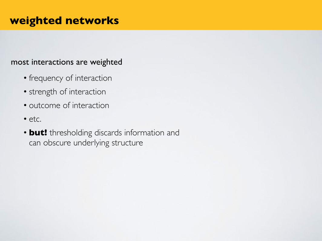
weighted networks
most interactions are weighted
• frequency of interaction• strength of interaction• outcome of interaction• etc.• but! thresholding discards information and
can obscure underlying structure
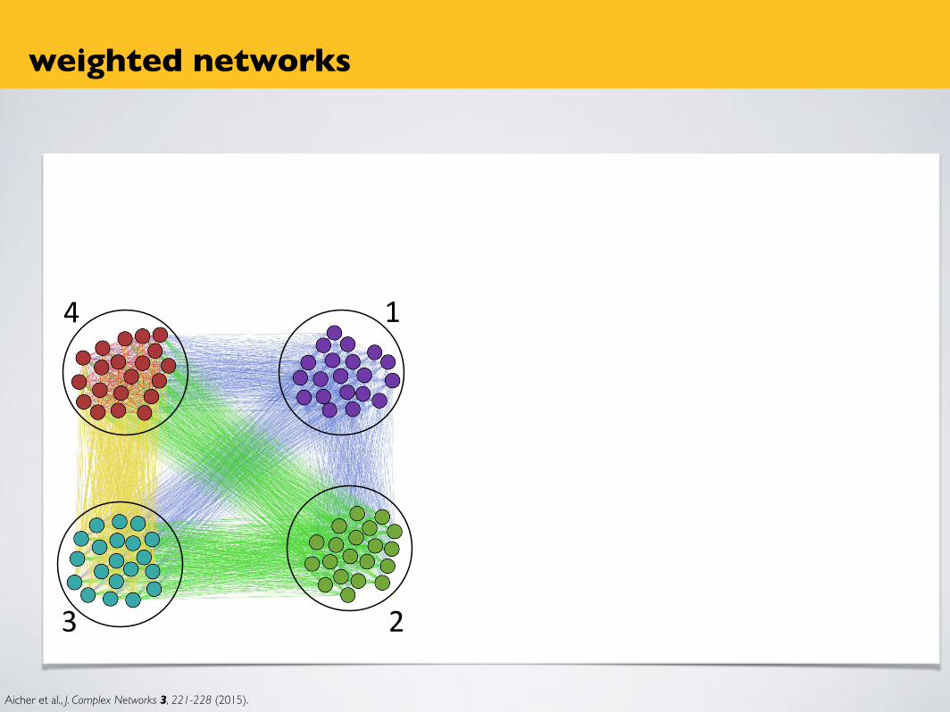
weighted networks
Aicher et al., J. Complex Networks 3, 221-228 (2015).
1
2
4
3

weighted networks
Aicher et al., J. Complex Networks 3, 221-228 (2015).
Threshold = 3 Threshold = 2 Threshold = 1 Threshold = 4
1
2
4
3
weighted networks
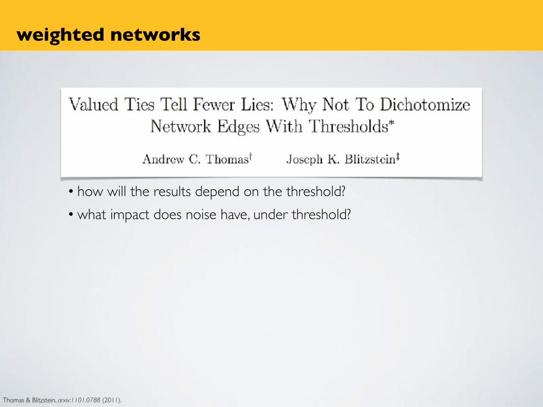
Thomas & Blitzstein, arxiv:1101.0788 (2011).
• how will the results depend on the threshold?• what impact does noise have, under threshold?
✓a,⇤
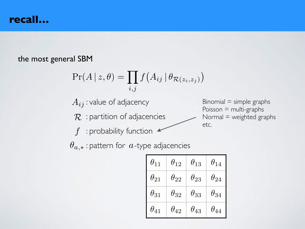
the most general SBM
recall…
Pr(A | z, ✓) =Y
i,j
f�Aij | ✓R(zi,zj)
�
f
RAij : value of adjacency
: partition of adjacencies
: probability function
: pattern for -type adjacencies
Binomial = simple graphsPoisson = multi-graphsNormal = weighted graphsetc.
a
✓11
✓22
✓33
✓44
✓12
✓21
✓31 ✓32
✓41 ✓42 ✓43
✓34
✓24
✓14✓13
✓23
weighted networks
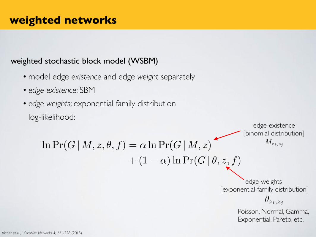
weighted stochastic block model (WSBM)
• model edge existence and edge weight separately• edge existence: SBM• edge weights: exponential family distribution
log-likelihood:
Poisson, Normal, Gamma, Exponential, Pareto, etc.
edge-existence[binomial distribution]
edge-weights [exponential-family distribution]
Mzi,zj
✓zi,zj
ln Pr(G |M, z, ✓, f) = ↵ ln Pr(G |M, z)
+ (1� ↵) lnPr(G | ✓, z, f)
Aicher et al., J. Complex Networks 3, 221-228 (2015).
weighted networks
weighted stochastic block model (WSBM)
• model edge existence and edge weight separately• edge existence: SBM• edge weights: exponential family distribution
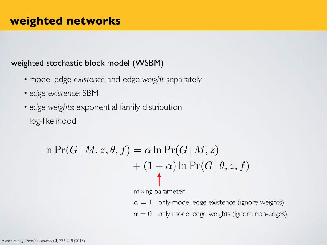
log-likelihood:
mixing parameter
ln Pr(G |M, z, ✓, f) = ↵ ln Pr(G |M, z)
+ (1� ↵) lnPr(G | ✓, z, f)
Aicher et al., J. Complex Networks 3, 221-228 (2015).
↵ = 1
↵ = 0
only model edge existence (ignore weights)only model edge weights (ignore non-edges)
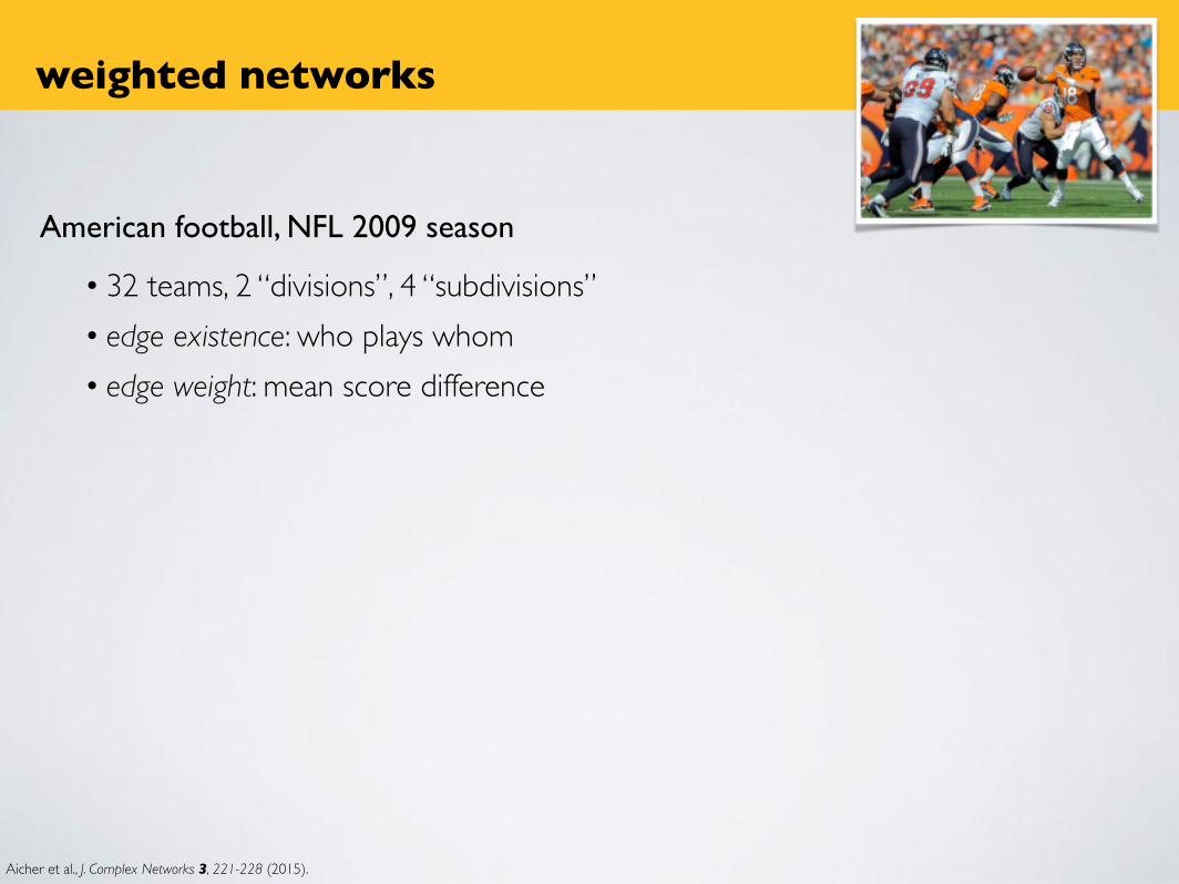
American football, NFL 2009 season
• 32 teams, 2 “divisions”, 4 “subdivisions”• edge existence: who plays whom• edge weight: mean score difference
weighted networks
Aicher et al., J. Complex Networks 3, 221-228 (2015).
{{
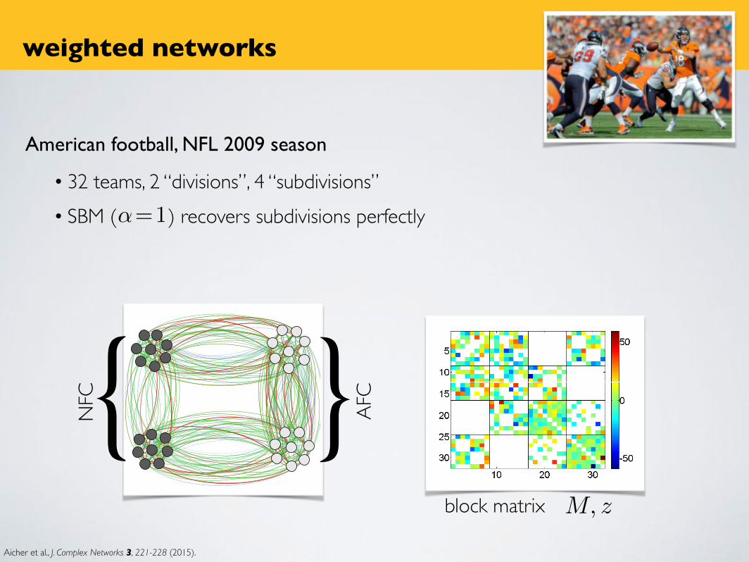
American football, NFL 2009 season
• 32 teams, 2 “divisions”, 4 “subdivisions”• SBM ( ) recovers subdivisions perfectly
NFC AFC
block matrix M, z
↵=1
weighted networks
Aicher et al., J. Complex Networks 3, 221-228 (2015).
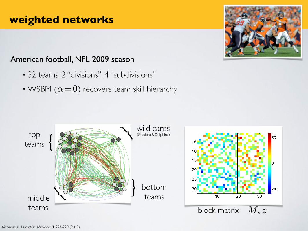
American football, NFL 2009 season
• 32 teams, 2 “divisions”, 4 “subdivisions”• WSBM ( ) recovers team skill hierarchy↵=0
{topteams
bottomteams
{middleteams
{
{ wild cards
block matrix M, z
weighted networks
(Steelers & Dolphins)
Aicher et al., J. Complex Networks 3, 221-228 (2015).

weighted networks
adding weights to the SBM
• what does mean?no edge or weight=0 edge or non-observed edge?
• how will we model the distribution of edge weights? • edge existences and edge weights may contain different large-scale structure
(conference structure vs. skill hierarchy)
Aij = 0

other approaches
weighted networks
other approaches
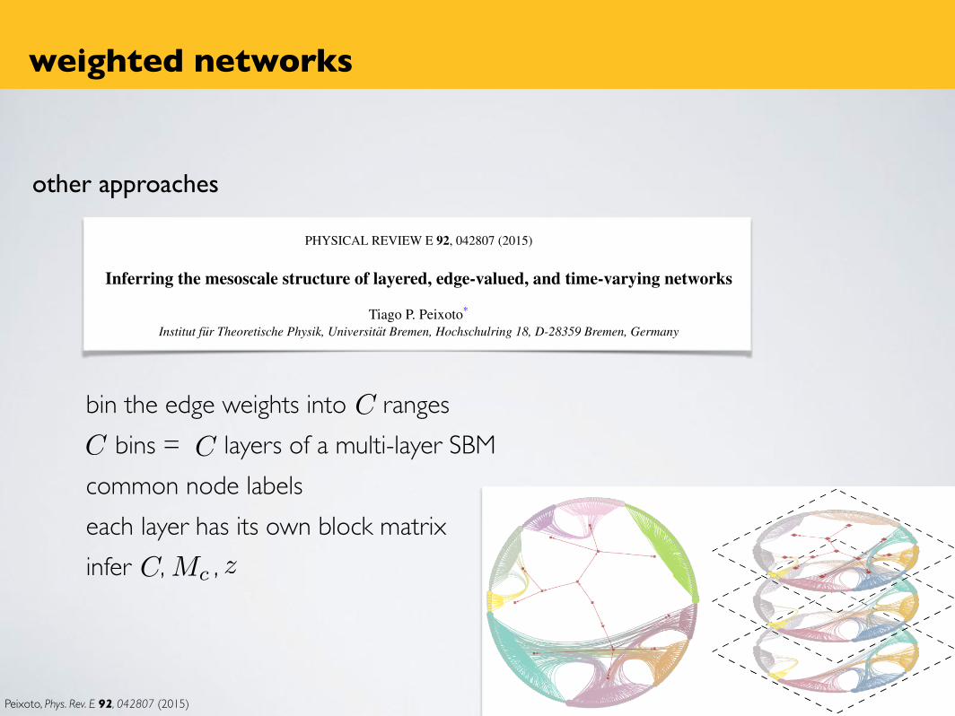
bin the edge weights into ranges bins = layers of a multi-layer SBMcommon node labelseach layer has its own block matrixinfer , ,
Peixoto, Phys. Rev. E 92, 042807 (2015)
PHYSICAL REVIEW E 92, 042807 (2015)
Inferring the mesoscale structure of layered, edge-valued, and time-varying networks
Tiago P. Peixoto*
Institut fur Theoretische Physik, Universitat Bremen, Hochschulring 18, D-28359 Bremen, Germany(Received 18 June 2015; published 9 October 2015)
Many network systems are composed of interdependent but distinct types of interactions, which cannot befully understood in isolation. These different types of interactions are often represented as layers, attributes onthe edges, or as a time dependence of the network structure. Although they are crucial for a more comprehensivescientific understanding, these representations offer substantial challenges. Namely, it is an open problem how toprecisely characterize the large or mesoscale structure of network systems in relation to these additional aspects.Furthermore, the direct incorporation of these features invariably increases the effective dimension of the networkdescription, and hence aggravates the problem of overfitting, i.e., the use of overly complex characterizationsthat mistake purely random fluctuations for actual structure. In this work, we propose a robust and principledmethod to tackle these problems, by constructing generative models of modular network structure, incorporatinglayered, attributed and time-varying properties, as well as a nonparametric Bayesian methodology to infer theparameters from data and select the most appropriate model according to statistical evidence. We show that themethod is capable of revealing hidden structure in layered, edge-valued, and time-varying networks, and thatthe most appropriate level of granularity with respect to the additional dimensions can be reliably identified. Weillustrate our approach on a variety of empirical systems, including a social network of physicians, the votingcorrelations of deputies in the Brazilian national congress, the global airport network, and a proximity networkof high-school students.
DOI: 10.1103/PhysRevE.92.042807 PACS number(s): 89.75.Hc, 02.50.Tt, 89.70.Cf
I. INTRODUCTION
The network abstraction has been successfully used as apowerful framework behind the modeling of a great variety ofbiological, technological, and social systems [1]. Traditionally,most network models proposed in these contexts consistof a set of elements possessing a single type of pairwiseinteraction (e.g., epidemic contact, transport route, metabolicreaction, etc.). More recently, it has becoming increasinglyclear that single types of interaction do not occur in isolation,and that a complete system encompasses several layers ofinteractions [2–4], and very often change in time [5]. Manyexamples have shown that the interplay between differenttypes of interactions can dramatically change the outcomeof paradigmatic processes such as percolation [6], epi-demic spreading [7–9], diffusion [10,11], opinion formation[12–14], evolutionary games [15–17], and synchroniza-tion [3,18], among others. The realization that different typesof interaction need to be incorporated into network modelsalso changes the way data need to be analyzed. In particular,the large or mesoscale structure of network systems may beintertwined with the layered or temporal structure, in such away that cannot be visible if this information is omitted. Theconventional approach of representing mesoscale structures isto separate the nodes into groups (or modules, “communities”)that have a similar role in the network topology [19]. Somemethods have been proposed to identify such groups in bothlayered [4,20–22] and time-varying [20,21,23–28] networks.However, these methods do not address two very central ques-tions: (1) Is the layered or temporal structure indeed importantfor the description of the network and, if so, to what degree ofgranularity? (2) How does one distinguish between multiple
descriptions of the same network, and in particular separateactual structure from stochastic fluctuations? In this work,we tackle both of these questions by formulating generativemodels of layered networks, obtained by generalizing severalvariants of the stochastic block model [29–32], incorporatingfeatures such as hierarchical structure [33,34], overlappinggroups [35–37], and degree correction [38], in additionto different types of layered structure. We show how theunsuspecting incorporation of many layers that happen to beuncorrelated with the mesoscale structure can, in fact, hinderthe detection task and obscure structure that would be visibleby ignoring the layer division in the usual fashion. Since mostmethods proposed so far take any available layer informationfor granted and attempt to model it in absolute detail, this issuerepresents a severe limitation of these methods in capturingthe structure of layered networks in a reliable manner. Weshow how this problem can be solved by performing modelselection under a general nonparametric Bayesian framework,which can also be used to select between different modelflavors (e.g., with overlapping groups or degree correction).We demonstrate that the proposed methodology can also beused to infer mesoscale structure in networks with real-valuedcorrelates on the edges (such as weights, distances, etc.), whilereliably distinguishing structure from noise, as well as changepoints in time-varying networks [39].
This work extends recent developments on layered [40–45],edge-valued [46–49], and temporal [50–54] generative pro-cesses, not only by incorporating many important topologicalpatterns simultaneously (i.e., hierarchical structure, degreecorrection, and overlapping groups), but also by tying allof these types of models into a nonparametric Bayesianframework that permits model selection and avoids overfitting.The framework presented allows one not only to select amongall different model classes, but also their appropriate order, i.e.,the number of groups, layer bins, and hierarchical structure.
1539-3755/2015/92(4)/042807(15) 042807-1 ©2015 American Physical Society
INFERRING THE MESOSCALE STRUCTURE OF LAYERED, . . . PHYSICAL REVIEW E 92, 042807 (2015)
FIG. 4. (Color online) Two generative models for a layeredsocial network of physicians [67]. (a) Inferred DCSBM for thecollapsed network, with the edges assumed to be randomly distributedamong the layers. (b) Inferred DCSBM with edge covariates, whereeach layer corresponds to one type of acquaintance. Below eachfigure is shown the posterior odds ratio !, relative to preferredmodel (a). The circular layout with edge bundling [68] representsthe inferred node hierarchy (indicated also by the red nodes andedges), as explained in the text (see also Ref. [34]).
there is enough evidence to justify the incorporation of layersthat are correlated with the group structure.
As a concrete example, here we consider an empiricalsocial network of N = 241 physicians, collected during asurvey [67]. Participants were asked which other physiciansthey would contact in hypothetical situations. The questionsasked were as follows: (1) When you need information oradvice about questions of therapy, where do you usually turn?(2) And who are the three or four physicians with whom youmost often find yourself discussing cases or therapy in thecourse of an ordinary week—last week for instance? (3) Wouldyou tell me the first names of your three friends whom you seemost often socially? The answers to each question representedges in one specific layer of a directed network. If one appliesthe DCSBM to the collapsed graph (which provides the best fitamong the alternatives), it yields a division into B = 9 groups,as shown in the left panel of Fig. 4, including also a divisioninto three disconnected components (corresponding to differ-ent cities). Between the layered SBM versions, the model withedge covariates turns out to be a better fit to the data (i.e., yieldsa lower description length) and divides the network into B = 8groups, as shown in the left panel of Fig. 4. When inspectingthe edge counts visually, one does not notice any significantdifference between the patterns in each layer. Indeed, whencomparing the description lengths between the null model withrandom layers above and the SBM with edge covariates, wefind that the latter is strongly rejected with a posterior oddsratio ! ≈ 10−51. Therefore, there is no noticeable evidence inthe data to support any correlation of layer divisions with thelarge-scale structure present in the graph. This suggests thatthe important descriptors of this social network are mainlythe overall acquaintances among physicians, not their precisetypes (at least as measured by the survey questions).
We now turn to another example, where informative layeredstructure can be detected. We consider the vote correlationnetwork of federal deputies in the Brazilian national congress.Based on public data containing the votes of all deputies in
all chamber sessions across many years,3 we obtained thecorrelation matrix between all deputies. We constructed anetwork by connecting an edge from a deputy to other 10deputies with which that deputy is most correlated in theconsidered period.4 We then separated the network in twolayers, corresponding to two consecutive four-year terms,1999–2002 and 2003–2006. Deputies not present during thewhole period were removed from the network, yielding anetwork with N = 224 nodes and E = 7247 edges in total.When fitting the DCSBM for the collapsed network (which isagain the best model), we obtain the B = 11 partition shownin the left panel of Fig. 5. It shows a hierarchical division thatis largely consistent with party and coalition lines, as well aspositions in the political spectrum (with a noticeable deviationbeing a group of left-wing parties composed of PDT, PSB, andPCdoB that are grouped together with center-right parties PTBand PMDB). When incorporating the layers, the best modelfit is obtained by the DCSBM with independent layers, whichyields a B = 11 division mostly compatible with (but not fullyidentical to) the collapsed network, although with a differenthierarchical structure, as can be seen in the right panel of Fig. 5.However, the layered representation of this network reveals amajor coalition change between the two terms, consistent withthe shift of power that occurred with the election of a new pres-ident belonging to the previous main opposition party: In the1999–2002 term, we see a clear division into a government andopposition groups (as captured in the topmost level of the hier-archy), with most edges existing between groups of the samecamp, corresponding to a right-wing/center government led bythe PSDB, PMDB, PFL, DEM, and PP parties, and a left-wingopposition composed mostly of PT, PDT, PSB, and PCdoB. Af-ter 2002, we observe a shifted coalition landscape, with a left-wing/center government predominantly formed by PT, PMDB,PDT, PSB, and PCdoB, and an opposition led by PSDB,PFL, DEM, and PP. Because of this noticeable change in thelarge-scale network structure—that is completely erased in thecollapsed network—the null model with random layers endsup being forcefully rejected with ! ≈ 10−111, meaning that thelayered structure is very informative on the network structure.
In the above examples, we made a comparison between thelayered model and a null model with fully random layers. Insome scenarios, we might be interested in a more nuancedapproach, where the layers are coarse grained with a moreappropriate level of granularity. This can be done by mergingsome of the layers into bins, such that inside each bin the layermembership of the edges is distributed regardless of the groupstructure. Let ℓ specify a set of layers that were merged in onespecific bin, and {θ}{ℓ} be a shorthand for the possible set ofparameters of a layered SBM {Gℓ} (with independent layers oredge covariates) where each bin ℓ corresponds to an individuallayer. The likelihood of this model conditioned on a specificbin set {ℓ} is given by
P ({Gl}|{θ}{ℓ},{ℓ}) = P ({Gℓ}|{θ}{ℓ})!
ℓ
"l∈ℓ El!Eℓ!
, (17)
3Available at http://www.camara.gov.br/.4We experimented with other threshold values and obtained similar
results.
042807-7
C
CC
C Mc z
weighted networks
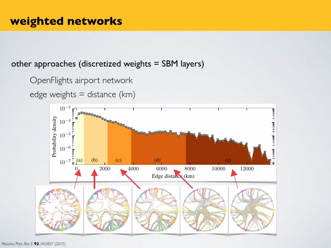
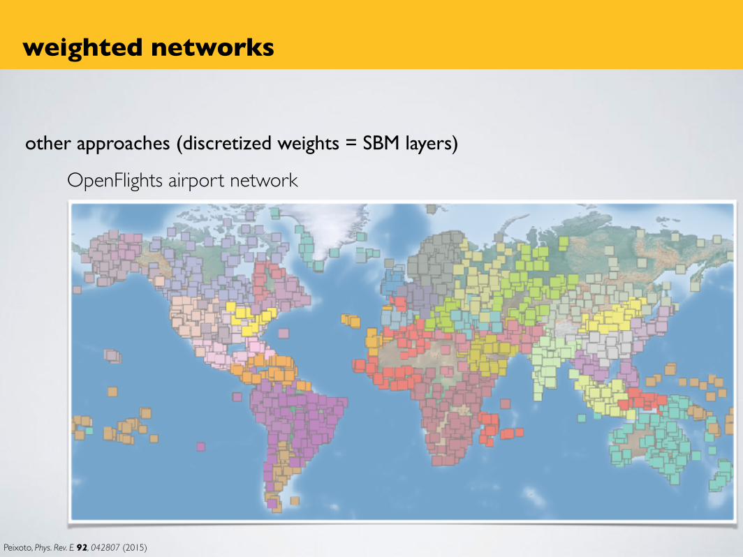
other approaches (discretized weights = SBM layers)
OpenFlights airport networkedge weights = distance (km)
Peixoto, Phys. Rev. E 92, 042807 (2015)
weighted networks
0 2000 4000 6000 8000 10000 12000
Edge distance (km)
10�7
10�6
10�5
10�4
10�3
Prob
abili
tyde
nsity
(a) (b) (c) (d) (e)
other approaches (discretized weights = SBM layers)
OpenFlights airport network
Peixoto, Phys. Rev. E 92, 042807 (2015)
weighted networks

fin
Related Documents


![Edld 5352 week01_assignmentjbuckels_ea1189[1]](https://static.cupdf.com/doc/110x72/548f3c36b4795991608b4791/edld-5352-week01assignmentjbuckelsea11891.jpg)
![[5352]-503 CEGP013091](https://static.cupdf.com/doc/110x72/61fa19cdf313ba794c314e19/5352-503-cegp013091.jpg)

