Lecture 3: Image Feature Extraction II Story so far - KTH · Lecture 3: Image Feature Extraction II Scanning an image sliding window image pyramid Interest points Harris point detector

Lecture 3: Image Feature Extraction II

Scanning an image

• sliding window• image pyramid

Interest points

• Harris point detector

Feature Extraction

• some odds and ends

Story so far

• Have introduced some methods to describe the appearance of an image patchvia a feature vector. (SIFT HOG etc..)

• For patches of similar appearance their computed feature vectors should besimilar while dissimilar if the patches differ in appearance.

• Feature vectors are designed to be invariant to common transformations thatsuperficially change the pixel appearance of the patch.

Next Problem

We have an reference image patch which is described by a feature vector fr.

Face Finder: Training• Positive examples:

– Preprocess ~1,000 example face images into 20 x 20 inputs

– Generate 15 “clones” of each with small random rotations, scalings, translations, reflections

• Negative examples– Test net on 120 known “no-face” images

��!��!��

��!��!��!��

⇒ fr

Given a novel image identify the patches in this image that correspond to thereference patch.

One part of the problem we have explored.

A patch from the novel image generates a feature vector fn. If ‖fr − fn‖ is

small then this patch can be considered an instance of the texture patternrepresented by the reference patch.

However, which and how many different image patches do we extractfrom the novel image ??

Remember..

The sought after image patch can appear at:

• any spatial location in the image

• any size, (the size of an imaged object depends on its from the camera)

• multiple locations

Variation in position and size- multiple detection windows

, 49

Sliding Window Technique

Therefore we must examine patches centered at many different pixel locations andat many different sizes.

Naive Option: Exhaustive search using original image

for j = 1:n sn = n min + j*n stepfor x=0:x maxfor y=0:y maxExtract image patch centred on pixel x, y of size n×n.Rescale it to the size of the reference patchCompute feature vector f.

This is computationally intensive especially if it is expensive to compute f as itcould be calculated upto n s × x max × y max.

Also frequently if n is large then it is very costly to compute f .

Scale Pyramid Option: Cleverer search

Construct an image pyramid that represents an image as several resolutions. Theneither

• Use the coarse scale to highlight promising image patches and then just explorethese area in more detail at the finer resolutions. (Quick but may miss bestimage patches)

• Visit every pixel in the fine resolution image as a potential centre pixel, butsimulate changing the window size by applying the same window size on thedifferent images in the pyramid.

Now will review construction of the image pyramid..

Naive Subsampling

6

SMOOTHED IMAGE NAIVE SUBSAMPLING

Pick every other pixel in both directions

SUBSAMPLING ARTIFACTS

Particularly noticeable in high frequency areas, such as on the hair. The lowest resolution level

represents very poorly the highest one.

SYNTHETIC EXAMPLE

1—D ALIASING

High frequency signal sampled at a much lower frequency.

2—D ALIASING

Sampling frequency lower than that of the signal yields a poor representation.

! Must remove high frequencies before sub-sampling.


Subsampling Artifacts

6






SYNTHETIC EXAMPLE

1—D ALIASING


2—D ALIASING



Particularlynoticeable in highfrequency areas,

such as on the hair.

Synthetic Example

6






SYNTHETIC EXAMPLE

1—D ALIASING


2—D ALIASING



Under-sampling

Undersampling

• Looks just like lower frequency signal!

Undersampling

• Looks like higher frequency signal!

Aliasing: higher frequency information can appear as lower frequency information

Undersampling

Good sampling

Bad sampling

Aliasing

AliasingInput signal:

x = 0:.05:5; imagesc(sin((2.^x).*x))

Matlab output:

Not enough samples

Aliasing in video

Slide credit: S. Seitz

Looks just like a lower frequency signal!

Under-samplingUndersampling

• Looks just like lower frequency signal!

Undersampling

• Looks like higher frequency signal!


Undersampling

Good sampling

Bad sampling

Aliasing

AliasingInput signal:

x = 0:.05:5; imagesc(sin((2.^x).*x))

Matlab output:

Not enough samples

Aliasing in video

Slide credit: S. Seitz

Looks like higher frequency signal!


2-D Aliasing

6






SYNTHETIC EXAMPLE

1—D ALIASING


2—D ALIASING



High frequency signalsampled lower than that

of the signal yields apoor representation.Therefore mustremove high

frequencies beforesub-sampling.

Aliasing Summary

• Can’t shrink an image by taking every second pixel due to sampling below theNyquist rate

• If we do, characteristic errors appear such as

– jaggedness in line features– spurious highlights– appearance of frequency patterns not present in the original image

Gaussian Pyramid

7

GAUSSIAN PYRAMID

• Gaussian smooth• Pick every other pixel in both directions

LOSS OF DETAILS BUT NOT ARTIFACTS

!No aliasing but details are lost as high frequencies are progressively removed.

LAPLACIAN PYRAMID

Each level of the Laplacian pyramid is the difference between corresponding and next higher level of the Gaussian Pyramid.

LAPLACIAN RECONSTRUCTION

• Upsampling by interpolation.• Adding upsampled image and difference image.

P. Burt and E. Adelson, The Laplacian Pyramid as a Compact Image Code, IEEE Transactions on Communications, 1983.

LAPLACIAN PYRAMID

• Pixels in the difference images are relatively uncorrelated.

• Their values are concentrated around zero.

ENTROPY AND QUANTIZATION

! Effective compression through shortened and variable code words.

• Gaussian smooth image

• Pick every other pixel in both directions

Images in the Pyramid

7

GAUSSIAN PYRAMID

• Gaussian smooth• Pick every other pixel in both directions

LOSS OF DETAILS BUT NOT ARTIFACTS

!No aliasing but details are lost as high frequencies are progressively removed.

LAPLACIAN PYRAMID

Each level of the Laplacian pyramid is the difference between corresponding and next higher level of the Gaussian Pyramid.

LAPLACIAN RECONSTRUCTION

• Upsampling by interpolation.• Adding upsampled image and difference image.

P. Burt and E. Adelson, The Laplacian Pyramid as a Compact Image Code, IEEE Transactions on Communications, 1983.

LAPLACIAN PYRAMID

• Pixels in the difference images are relatively uncorrelated.

• Their values are concentrated around zero.

ENTROPY AND QUANTIZATION

! Effective compression through shortened and variable code words.

No aliasing but detailsare lost as highfrequencies are

progressively removed.

Scaled representation advantages

• Find template matches at all scales

– Template size is constant, but image size changes

• Efficient search for correspondence

– look at coarse scales, then refine with finer scales– much less cost, but may miss best match

• Examining of all levels of detail

– Find edges with different amounts of blur– Find textures with different spatial frequencies

Still too slow ??Even if using an image pyramid representation, very many pixel locations still mayhave to be visited. This requires many calculations of a potentially expensivefeature vector. Perhaps too many for a real-time application or for searchingthousands/millions of images in a reasonable amount of time.

Some people propose another approach based on the concept of interest points.

Intuition

There is a subset of points of an image, interest points, representing some kind ofspecific image structure that can be found reliably and consistently across imageseven when the structure undergoes rotation and scale changes.

Reference image patches are then chosen such that interest points are at theircentres.

Then given a novel image the interest point detector produces estimates {xi, yi, ni}

of the position and size of the image patch. The number of these candidates willgenerally be much less than the number of pixels in an image.

An Interest PointAn interest point is a point in the image which can be characterized it has

• a clear, preferably mathematically well-founded, definition

• a well-defined position in image space

• the local image structure around the interest point is rich in terms of localinformation contents, such that the use of interest points simplify furtherprocessing in the vision system

• it is stable under local and global perturbations in the image domain, includingdeformations as those arising from perspective transformations (sometimesreduced to affine transformations, scale changes, rotations and/or translations)as well as illumination/brightness variations, such that the interest points canbe reliably computed with high degree of reproducibility.

• the notion of interest point should include an attribute of scale, to makeit possible to compute interest points from real-life images which of courseundergo scale changes.

The Harris Corner Detector

The Harris corner, though not invariant to scale, is the basis for one such scaleinvariant interest point detector.

! ⇥!⇤⌅⇧⌃⌥!⌅⌥! ⌦↵,⌅!.↵,✏⌦⌅⇣⌘!✓⌦◆!⇧⌃!56⇣↵⌫◆↵⌦!⇠⇧⌫⇡5⇣↵,⇢⌘!;,⌧⇣↵⇣5⇣!⌃=⌅!;,⌃⇧⌅⌫⌦⇣↵>⌘!?,↵@⌅⌧↵⇣!⇣!"5⇢⌧#5⌅⇢!!$↵%✏6↵⇣,⌅⌧⇣⌅⌥!&'⌘!()*+&,!"5⇢⌧#5⌅⇢⌘!-⌅⌫⌦,./!⌫⌦↵60! ⌦↵,⌅⌥.↵,✏⌦⌅⇣1↵,⌃⇧⌅⌫⌦⇣↵>⌥5,↵(⌦5⇢⌧#5⌅⇢⌥◆

! ⌃⌅ %⇤✏⇣%⇤⌘⌃⌦✓⇥◆1⌦2

⇠⌥✓⌦⌅⌅↵⌧⌘!⌥2⇣⇡✏,⌧⌥!3"!⇠⇧⌫#↵,◆!⇠⇧⌅,⌅!⌦,◆!$◆⇢!⇣%⇣⇧⌅4⌥!+5))

C.Harris, M.Stephens. A Combined Corner and Edge Detector. 1988

The Basic Idea 1

• We should easily recognize the point by looking through a small window.

• Shifting a window in any direction should give a large change in intensity.

! ⇥!⇤⌅⇧⌃⌥!⌅⌥! ⌦↵,⌅!.↵,✏⌦⌅⇣⌘!✓⌦◆!⇧⌃!56⇣↵⌫◆↵⌦!⇠⇧⌫⇡5⇣↵,⇢⌘!;,⌧⇣↵⇣5⇣!⌃=⌅!;,⌃⇧⌅⌫⌦⇣↵>⌘!?,↵@⌅⌧↵⇣!⇣!"5⇢⌧#5⌅⇢!!$↵%✏6↵⇣,⌅⌧⇣⌅⌥!&'⌘!()*+&,!"5⇢⌧#5⌅⇢⌘!-⌅⌫⌦,./!⌫⌦↵60! ⌦↵,⌅⌥.↵,✏⌦⌅⇣1↵,⌃⇧⌅⌫⌦⇣↵>⌥5,↵(⌦5⇢⌧#5⌅⇢⌥◆

⌫⇠⌦⌃⇡⇥⇧⌅⌃⇢✏⌦⇥

⇥ !⇥⇤⌅⇧⌃⌥ ⇤⇥⌦⌅↵,⇤⇥.⌃✏⇣↵⌘⇥⇤✓⇧⇥⇤◆⌃↵⇣✓⇤,⇤⌃⌃5↵⇣✏⇤✓⇧⌃⌥✏⇧⇤⌦⇤⌅6⌦⇤⌫↵⇣ ⌃⌫

⇥ ⇠⇧↵⇡✓↵⇣✏⇤⌦⇤⌫↵⇣ ⌃⌫⇤↵⇣⇤!⇥⇤⇤⌅⇧⌃⌥ ⇧⌦⇥⇤⌅⇧⌃⌥ ⇤✏↵⇢⇥⇤!↵,!⌃⌥↵.!⇥⌥⇤↵⇣⇤↵⇣✓⇥⇣⌅↵✓,

The Basic Idea 2

! ⇥!⇤⌅⇧⌃⌥!⌅⌥! ⌦↵,⌅!.↵,✏⌦⌅⇣⌘!✓⌦◆!⇧⌃!56⇣↵⌫◆↵⌦!⇠⇧⌫⇡5⇣↵,⇢⌘!;,⌧⇣↵⇣5⇣!⌃=⌅!;,⌃⇧⌅⌫⌦⇣↵>⌘!?,↵@⌅⌧↵⇣!⇣!"5⇢⌧#5⌅⇢!!$↵%✏6↵⇣,⌅⌧⇣⌅⌥!&'⌘!()*+&,!"5⇢⌧#5⌅⇢⌘!-⌅⌫⌦,./!⌫⌦↵60! ⌦↵,⌅⌥.↵,✏⌦⌅⇣1↵,⌃⇧⌅⌫⌦⇣↵>⌥5,↵(⌦5⇢⌧#5⌅⇢⌥◆

⇡⇥⇧⌅⌃⇢✏⌦⇥⌃*⌧,

3⌃6⌦⇣4!⌅⇢↵⇧,0,⇧!%✏⌦,⇢!↵,!⌦66!◆↵⌅%⇣↵⇧,⌧

3◆⇢40,⇧!%✏⌦,⇢!⌦6⇧,⇢!⇣✏!◆⇢!◆↵⌅%⇣↵⇧,

3%⇧⌅,⌅40⌧↵⇢,↵⌃↵%⌦,⇣!%✏⌦,⇢!↵,!⌦66!◆↵⌅%⇣↵⇧,⌧

Mathematics

Change in the intensity for a shift (u, v):

E(u, v) =∑

(x,y)∈W

w(x, y) [I(x + u, y + v)− I(x, y)]2

where the weight mask w(x, y) is either:

! ⇥!⇤⌅⇧⌃⌥!⌅⌥! ⌦↵,⌅!.↵,✏⌦⌅⇣⌘!✓⌦◆!⇧⌃!56⇣↵⌫◆↵⌦!⇠⇧⌫⇡5⇣↵,⇢⌘!;,⌧⇣↵⇣5⇣!⌃=⌅!;,⌃⇧⌅⌫⌦⇣↵>⌘!?,↵@⌅⌧↵⇣!⇣!"5⇢⌧#5⌅⇢!!$↵%✏6↵⇣,⌅⌧⇣⌅⌥!&'⌘!()*+&,!"5⇢⌧#5⌅⇢⌘!-⌅⌫⌦,./!⌫⌦↵60! ⌦↵,⌅⌥.↵,✏⌦⌅⇣1↵,⌃⇧⌅⌫⌦⇣↵>⌥5,↵(⌦5⇢⌧#5⌅⇢⌥◆

!⇥#⇠⌦◆⇥#⌅⇧

*⇥⇤⇤⌅⇧⌃↵⌦#⌦#⇤/⌃

!⇥#⇠⌦◆⇥#⌅⇧

⇠✏⌦,⇢!⇧⌃!↵,⇣,⌧↵⇣.!⌃⇧⌅!⇣✏!⌧✏↵⌃⇣!6!⇥⇤70

!⇥⇤⌅⇥⇧⌃⇤⌥ ⌃⌦⇤⌅↵,⌃⇥⇤⌅⇥⇧⌃⇤⌥

⌃⇥↵.✏,⌦⇣⇥⌘⇤⌃.⇥

⇧⌅8↵,◆⇧9!⌃5,%⇣↵⇧,!⌅⇧⌃⇥⌥!:

-⌦5⌧⌧↵⌦,+!↵,!9↵,◆⇧9⌘!'!⇧5⇣⌧↵◆

! !⇥ ⇤ ⌅⇥⇤⌅⇧ ⇤ ⌃

⌥! ⇧ ⇤ ⌃⇥⇧ !⇧⌃⇥ ⇤ ⌃⌃⌅ ⇥⌥ ! ⇧ ⇤ ⌃⇥⇤

Mathematics

For small shifts (u, v) we have a bilinear approximation:

E(u, v) ≈ (u, v) M

(uv

)where M is a 2× 2 matrix computed from image derivatives:

M =∑

(x,y)∈W

w(x, y)(

Ix(x, y)2 Ix(x, y)Iy(x, y)Ix(x, y)Iy(x, y) Iy(x, y)2

)

Mathematics

Intensity change in shifting window: use eigenvalue analysis

Let λ1 and λ2 be the eigenvalues of M .

! ⇥!⇤⌅⇧⌃⌥!⌅⌥! ⌦↵,⌅!.↵,✏⌦⌅⇣⌘!✓⌦◆!⇧⌃!56⇣↵⌫◆↵⌦!⇠⇧⌫⇡5⇣↵,⇢⌘!;,⌧⇣↵⇣5⇣!⌃=⌅!;,⌃⇧⌅⌫⌦⇣↵>⌘!?,↵@⌅⌧↵⇣!⇣!"5⇢⌧#5⌅⇢!!$↵%✏6↵⇣,⌅⌧⇣⌅⌥!&'⌘!()*+&,!"5⇢⌧#5⌅⇢⌘!-⌅⌫⌦,./!⌫⌦↵60! ⌦↵,⌅⌥.↵,✏⌦⌅⇣1↵,⌃⇧⌅⌫⌦⇣↵>⌥5,↵(⌦5⇢⌧#5⌅⇢⌥◆

⌃"⇥$⇠⌦◆⇥$⌅⇧

;,⇣,⌧↵⇣.!%✏⌦,⇢!↵,!⌧✏↵⌃⇣↵,⇢!9↵,◆⇧90!↵⇢,@⌦65!⌦,⌦6.⌧↵⌧

λ+⌘!λ=!>!↵⇢,@⌦65⌧!⇧⌃!⇣

!⇥⇤⌅⇧⌃⇥⌥ ⌥⌦ ⌃↵⌅ ,⌥.⌅,⌃ ⇧↵✏⇣⌅

!⇥⇤⌅⇧⌃⇥⌥ ⌥⌦ ⌃↵⌅ ⌦✏,⌃⌅,⌃ ⇧↵✏⇣⌅

?λ⌫⌦<@(+A=

?λ⌫↵,@(+A=

$66↵⇡⌧!⌘⇧$⇥⇤✓:!%⇧,⌧⇣

⇤⌅⇧ ⇤ ⌃

⌥# ⇧ ⇤ ⌃⇥⇧ ⇧⇤

⇧ ⌃

⇧ ⌃ ⌃⇤

! ⇥!⇤⌅⇧⌃⌥!⌅⌥! ⌦↵,⌅!.↵,✏⌦⌅⇣⌘!✓⌦◆!⇧⌃!56⇣↵⌫◆↵⌦!⇠⇧⌫⇡5⇣↵,⇢⌘!;,⌧⇣↵⇣5⇣!⌃=⌅!;,⌃⇧⌅⌫⌦⇣↵>⌘!?,↵@⌅⌧↵⇣!⇣!"5⇢⌧#5⌅⇢!!$↵%✏6↵⇣,⌅⌧⇣⌅⌥!&'⌘!()*+&,!"5⇢⌧#5⌅⇢⌘!-⌅⌫⌦,./!⌫⌦↵60! ⌦↵,⌅⌥.↵,✏⌦⌅⇣1↵,⌃⇧⌅⌫⌦⇣↵>⌥5,↵(⌦5⇢⌧#5⌅⇢⌥◆

⌃"⇥$⇠⌦◆⇥$⌅⇧

λ+

λ=

3⇠⇧⌅,⌅4

λ+!⌦,◆!λ=!⌦⌅!6⌦⌅⇢⌘!λ+!B!λ=/⌘!↵,%⌅⌦⌧⌧!↵,!⌦66!◆↵⌅%⇣↵⇧,⌧

λ+!⌦,◆!λ=!⌦⌅!⌧⌫⌦66/⌘!↵⌧!⌦6⌫⇧⌧⇣!%⇧,⌧⇣⌦,⇣!↵,!⌦66!◆↵⌅%⇣↵⇧,⌧

3$◆⇢4!

λ+!CC!λ=

3$◆⇢4!

λ=!CC!λ+

3;6⌦⇣4!⌅⇢↵⇧,

⇠6⌦⌧⌧↵⌃↵%⌦⇣↵⇧,!⇧⌃!↵⌫⌦⇢!⇡⇧↵,⇣⌧!5⌧↵,⇢!↵⇢,@⌦65⌧!⇧⌃!⇣0

Mathematics

Measure of corner response:

R = det(M)− κ (trace(M))2

where

det(M) = λ1λ2

trace(M) = λ1 + λ2

κ is a constant whose value was determined empirically to give results in the range[.04, .06].

! ⇥!⇤⌅⇧⌃⌥!⌅⌥! ⌦↵,⌅!.↵,✏⌦⌅⇣⌘!✓⌦◆!⇧⌃!56⇣↵⌫◆↵⌦!⇠⇧⌫⇡5⇣↵,⇢⌘!;,⌧⇣↵⇣5⇣!⌃=⌅!;,⌃⇧⌅⌫⌦⇣↵>⌘!?,↵@⌅⌧↵⇣!⇣!"5⇢⌧#5⌅⇢!!$↵%✏6↵⇣,⌅⌧⇣⌅⌥!&'⌘!()*+&,!"5⇢⌧#5⌅⇢⌘!-⌅⌫⌦,./!⌫⌦↵60! ⌦↵,⌅⌥.↵,✏⌦⌅⇣1↵,⌃⇧⌅⌫⌦⇣↵>⌥5,↵(⌦5⇢⌧#5⌅⇢⌥◆

⌃"⇥$⇠⌦◆⇥$⌅⇧

λ+

λ= 3⇠⇧⌅,⌅4

3$◆⇢4!

3$◆⇢4!

3;6⌦⇣4

⇥!!◆⇡,◆⌧!⇧,6.!⇧,!↵⇢,@⌦65⌧!⇧⌃!

⇥!!↵⌧!6⌦⌅⇢!⌃⇧⌅!⌦!%⇧⌅,⌅

⇥!!↵⌧!,⇢⌦⇣↵@!9↵⇣✏!6⌦⌅⇢!⌫⌦⇢,↵⇣5◆!⌃⇧⌅!⌦,!◆⇢

⇥!EE!↵⌧!⌧⌫⌦66!⌃⇧⌅!⌦!⌃6⌦⇣!⌅⇢↵⇧,

!C!'

!F!'

!F!'""!⌧⌫⌦66

Harris Detector

The Algorithm:

• Find points with large corner response function R (R > threshold)

• Take the points of local maxima of R

Harris: In action

! ⇥!⇤⌅⇧⌃⌥!⌅⌥! ⌦↵,⌅!.↵,✏⌦⌅⇣⌘!✓⌦◆!⇧⌃!56⇣↵⌫◆↵⌦!⇠⇧⌫⇡5⇣↵,⇢⌘!;,⌧⇣↵⇣5⇣!⌃=⌅!;,⌃⇧⌅⌫⌦⇣↵>⌘!?,↵@⌅⌧↵⇣!⇣!"5⇢⌧#5⌅⇢!!$↵%✏6↵⇣,⌅⌧⇣⌅⌥!&'⌘!()*+&,!"5⇢⌧#5⌅⇢⌘!-⌅⌫⌦,./!⌫⌦↵60! ⌦↵,⌅⌥.↵,✏⌦⌅⇣1↵,⌃⇧⌅⌫⌦⇣↵>⌥5,↵(⌦5⇢⌧#5⌅⇢⌥◆

!⇥⇤⇤⌅⇧⌃↵⌦)⌦)⇤,⌃-⇤.!0"Harris: Corner Response

! ⇥!⇤⌅⇧⌃⌥!⌅⌥! ⌦↵,⌅!.↵,✏⌦⌅⇣⌘!✓⌦◆!⇧⌃!56⇣↵⌫◆↵⌦!⇠⇧⌫⇡5⇣↵,⇢⌘!;,⌧⇣↵⇣5⇣!⌃=⌅!;,⌃⇧⌅⌫⌦⇣↵>⌘!?,↵@⌅⌧↵⇣!⇣!"5⇢⌧#5⌅⇢!!$↵%✏6↵⇣,⌅⌧⇣⌅⌥!&'⌘!()*+&,!"5⇢⌧#5⌅⇢⌘!-⌅⌫⌦,./!⌫⌦↵60! ⌦↵,⌅⌥.↵,✏⌦⌅⇣1↵,⌃⇧⌅⌫⌦⇣↵>⌥5,↵(⌦5⇢⌧#5⌅⇢⌥◆

!⇥⇤⇤⌅⇧⌃↵⌦)⌦)⇤,⌃-⇤.!0"⇠⇧⌫⇡5⇣!%⇧⌅,⌅!⌅⌧⇡⇧,⌧!

Harris: Threshold

! ⇥!⇤⌅⇧⌃⌥!⌅⌥! ⌦↵,⌅!.↵,✏⌦⌅⇣⌘!✓⌦◆!⇧⌃!56⇣↵⌫◆↵⌦!⇠⇧⌫⇡5⇣↵,⇢⌘!;,⌧⇣↵⇣5⇣!⌃=⌅!;,⌃⇧⌅⌫⌦⇣↵>⌘!?,↵@⌅⌧↵⇣!⇣!"5⇢⌧#5⌅⇢!!$↵%✏6↵⇣,⌅⌧⇣⌅⌥!&'⌘!()*+&,!"5⇢⌧#5⌅⇢⌘!-⌅⌫⌦,./!⌫⌦↵60! ⌦↵,⌅⌥.↵,✏⌦⌅⇣1↵,⌃⇧⌅⌫⌦⇣↵>⌥5,↵(⌦5⇢⌧#5⌅⇢⌥◆

!⇥⇤⇤⌅⇧⌃↵⌦)⌦)⇤,⌃-⇤.!0";↵,◆!⇡⇧↵,⇣⌧!9↵⇣✏!6⌦⌅⇢!%⇧⌅,⌅!⌅⌧⇡⇧,⌧0!"⇣✏⌅⌧✏⇧6◆

Harris: Local Maxima

! ⇥!⇤⌅⇧⌃⌥!⌅⌥! ⌦↵,⌅!.↵,✏⌦⌅⇣⌘!✓⌦◆!⇧⌃!56⇣↵⌫◆↵⌦!⇠⇧⌫⇡5⇣↵,⇢⌘!;,⌧⇣↵⇣5⇣!⌃=⌅!;,⌃⇧⌅⌫⌦⇣↵>⌘!?,↵@⌅⌧↵⇣!⇣!"5⇢⌧#5⌅⇢!!$↵%✏6↵⇣,⌅⌧⇣⌅⌥!&'⌘!()*+&,!"5⇢⌧#5⌅⇢⌘!-⌅⌫⌦,./!⌫⌦↵60! ⌦↵,⌅⌥.↵,✏⌦⌅⇣1↵,⌃⇧⌅⌫⌦⇣↵>⌥5,↵(⌦5⇢⌧#5⌅⇢⌥◆

!⇥⇤⇤⌅⇧⌃↵⌦)⌦)⇤,⌃-⇤.!0"G⌦>!⇧,6.!⇣✏!⇡⇧↵,⇣⌧!⇧⌃!6⇧%⌦6!⌫⌦<↵⌫⌦!⇧⌃!

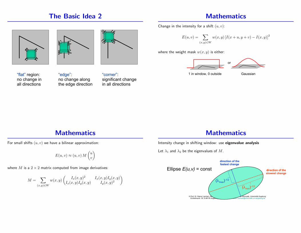
Harris: Final Points

! ⇥!⇤⌅⇧⌃⌥!⌅⌥! ⌦↵,⌅!.↵,✏⌦⌅⇣⌘!✓⌦◆!⇧⌃!56⇣↵⌫◆↵⌦!⇠⇧⌫⇡5⇣↵,⇢⌘!;,⌧⇣↵⇣5⇣!⌃=⌅!;,⌃⇧⌅⌫⌦⇣↵>⌘!?,↵@⌅⌧↵⇣!⇣!"5⇢⌧#5⌅⇢!!$↵%✏6↵⇣,⌅⌧⇣⌅⌥!&'⌘!()*+&,!"5⇢⌧#5⌅⇢⌘!-⌅⌫⌦,./!⌫⌦↵60! ⌦↵,⌅⌥.↵,✏⌦⌅⇣1↵,⌃⇧⌅⌫⌦⇣↵>⌥5,↵(⌦5⇢⌧#5⌅⇢⌥◆

!⇥⇤⇤⌅⇧⌃↵⌦)⌦)⇤,⌃-⇤.!0"Harris-Laplace Detector

The Harris corner detector is not invariant to scale changes. However, recent workdescribes how to extend the method to make it fire on the same structure evenacross large scale changes. This detector is called the Harris-Laplace detector

Scale & Affine Invariant Interest Point Detectors by K. Mikolajczyk and C.Schmid in International Journal of Computer Vision (2004)

This detector returns the position and the scale at which the interest point wasdetected.

80 Mikolajczyk and Schmid

Figure 12. Robust matching: Harris-Laplace detects 190 and 213 points in the left and right images, respectively (a). 58 points are initiallymatched (b). There are 32 inliers to the estimated homography (c), all of which are correct. The estimated scale factor is 4.9 and the estimatedrotation angle is 19 degrees.

Some results of the Harris-Laplace detector

Note the two images do contain some overlap.

(The SIFT paper also describes a method for finding scale invariant interest points.Their definition of interesting is different to that of Harris.)

Objects defined via interest pointsKeypoint detection

, 70

Some objects are defined by several interest points and associated image patches.

More on Feature extraction

Filter Banks

11

DERIVATIVES OF GAUSSIAN FILTERS

Measure the image gradient and its direction at different scales by using a pyramid.

HORIZONTAL AND VERTICAL STRUCTURES

FILTER BANKS

Represent image textures using the responses of a collection of filters. • An appropriate filter bank will extract useful

information such as spots and edges• Typically one or two spot filters plus several

oriented bar filters

FILTER RESPONSES

Based on the pixels with large magnitudes in the particular filter response, we can determine the presence of strong edges of certain orientation. We can also find spot patterns from the responses of the first two filters

FILTER RESPONSES:HIGH RESOLUTION

FILTER RESPONSES:LOW RESOLUTION

Represent an image patch especially using the responses of a collection of filters.

• An appropriate filter bank will extract useful information such as spots and edges

• Typically one or two spot filters plus several oriented bar filters

Filter Responses

11




FILTER BANKS




FILTER RESPONSES




Based on the pixels with large magnitudes in the particular filter response, we candetermine the presence of strong edges of certain orientation. We can also findspot patterns from the responses of the first two filters.

Filter Responses: High Resolution

11




FILTER BANKS




FILTER RESPONSES




Filter Responses: Low Resolution

11




FILTER BANKS




FILTER RESPONSES



FILTER RESPONSES:LOW RESOLUTION Filters as weighted sums

12

FILTERS AS WEIGHTED SUMS

Each filter is the sum of several weighted Gaussian filters:• The first spot filter is the sum of Gaussian filters with sigmas of 0.62, 1, and 1.6,

and weights of 1, -2, 1.• The second spot filter is the sum of Gaussian filters with sigmas of 0.71, 1.14,

and weights of 1, and –1• The six bar filters are rotated versions of a horizontal bar, which is the weighted

sum of three Gaussian filters, each has sigma_x of 2, and sigma_y of 1, with centers at (0,1), (0,0), and (0,-1)

QUERYING AN IMAGE DATABASE

IN SHORT

• Shift invariant linear operators can be expressed as convolutions.

• The Gaussian smoothing operator is an important special case.

• The Gaussian and Laplacian pyramids have numerous applications.

Each filter is the sum of several weighted Gaussian filters:

• The first spot filter is the sum of Gaussian filters with sigmas of 0.62, 1, and1.6, and weights of 1, -2, 1.

• The six bar filters are rotated versions of a horizontal bar, which is the weighted

sum of three Gaussian filters, each has σx of 2, and σy of 1, with centers at(0,1), (0,0), and (0,-1).

Steerable filtersSynthesize a filter of arbitrary orientation as a linear combination of basis filters.Let

Gθ1 = the first derivative of the Gaussian filter

in the x−direction rotated through angle θ

Then let

R0I = G0

1 ∗ I

R90I = G90

1 ∗ I

then

RθI = cos(θ) R0

I + sin(θ) R90I = Gθ

1 ∗ I

Interpolated filter responses more efficient than explicit filter at arbitrary orientation.

Freeman & Adelson, The Design and Use of SteerableFilters, PAMI 1991

Steerable filter: ExampleSteerable filters

=

=

Freeman & Adelson, 1991

Basis filters for derivative of Gaussian

[Torralba, Murphy, Freeman, and Rubin, ICCV 2003]

Probability of the scene given global features


Contextual priors

• Use scene recognition ! predict objects present

• For object(s) likely to be present, predict locations based on similarity to previous images with the same place and that object


Scene category

Specific place

(black=right, red=wrong)

Blue solid circle: recognition with temporal info

Black hollow circle: instantaneous recognition using global feature only

Cross: true location

Learning good boundaries

• Use ground truth (human-labeled) boundaries in natural images to

learn good features

• Supervised learning to optimize cue integration, filter scales, select

feature types

Work by D. Martin and C. Fowlkes and D. Tal and J. Malik, Berkeley Segmentation Benchmark,

2001

D. Martin et al. PAMI 2004

Training data


• Use ground truth (human-labeled) boundaries in natural images to learn good features

• Supervised learning to optimize cue integration, filter scales, select feature typesWork by D. Martin and C. Fowlkes and D. Tal and J. Malik, Berkeley Segmentation Benchmark, 2001

[D. Martin et al. PAMI 2004]

Human-marked segment boundaries

Feature profiles (oriented energy, brightness, color, and texture gradients) along the patch’s horizontal diameter


What features are responsible for perceived edges?




Original Boundary detection Human-labeled

Berkeley Segmentation Database, D. Martin and C. Fowlkes and D. Tal and J. Malik

Hand marked segment boundaries

Which features responsible for perceivededges ?

• oriented energy gradients (OE)

• brightness gradients (BG),

• color gradients (CG),

• texture gradients (TG)

1d profiles from patches














Patches containing no boundary

1d Profiles














Patches containing a boundary

After learning














More results


Edge detection and corners• Partial derivative estimates in x and y fail to

capture corners

Why do we care about corners?

Case study: panorama stitching

[Brown, Szeliski, and Winder, CVPR 2005]

How do we build panorama?

• We need to match (align) images

[Slide credit: Darya Frolova and Denis Simakov]

Matching with Features

• Detect feature points in both images

Matching with Features

• Detect feature points in both images

• Find corresponding pairs

Cosine Transformation

Given an image I(x, y) of size n×m. Then its cosine transform is defined by

q(k, l) =n−1∑x=0

m−1∑y=0

cos(

πkx

n

)cos

(πly

m

)I(x, y)

for k = 0, . . . , n− 1 and l = 0, . . . ,m− 1

Cosine Transformation Basis Cosine Transformation of Digits

Original Images

2D Discrete Cosine Transform

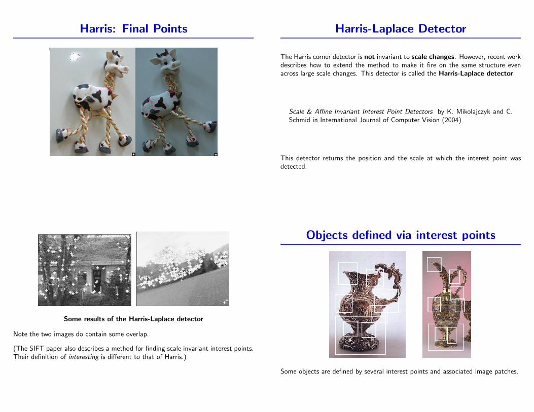
Fourier Transformation

Given an image I(x, y) of size n×m. Then its Fourier transform is defined by

q(k, l) =n−1∑x=0

m−1∑y=0

exp(

i2πkx

n

)exp

(i2πly

m

)I(x, y)

for k = 0, . . . , n− 1 and l = 0, . . . ,m− 1

Fourier Transformation of Digits

Original Images

Magnitude of the 2D Fourier Transform

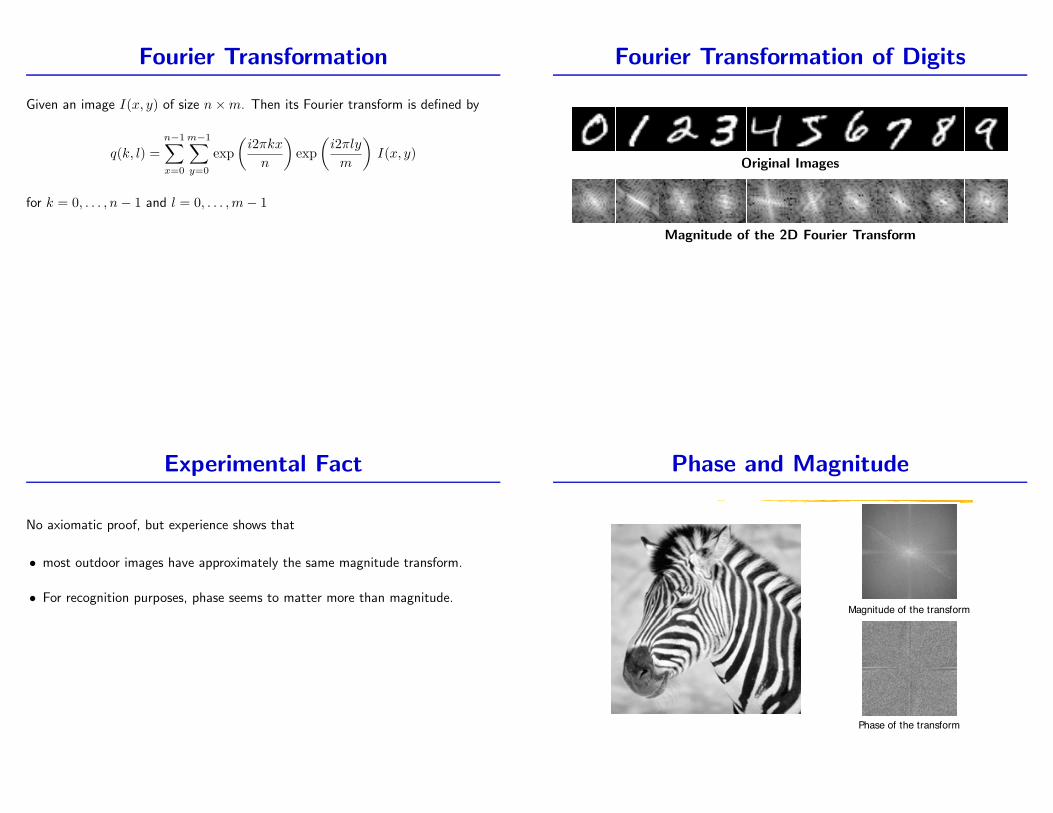
Experimental Fact

No axiomatic proof, but experience shows that

• most outdoor images have approximately the same magnitude transform.

• For recognition purposes, phase seems to matter more than magnitude.

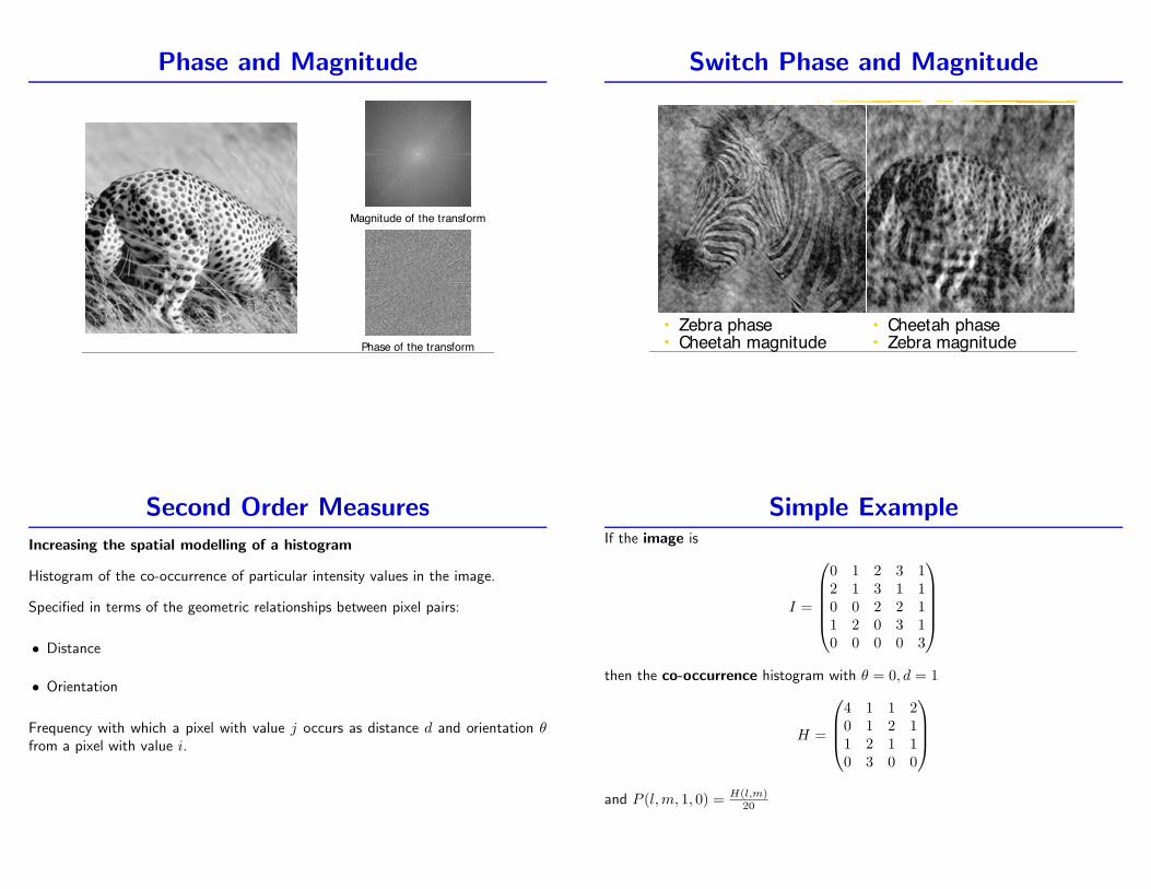
Phase and Magnitude

3

DFT OF 2-D ARRAY

))),(()),,((tan(: Phase

),( :Magnitude

vuFRvuFIa

vuF

Magnitude of the transform

Phase of the transform

PHASE AND MAGNITUDE



PHASE AND MAGNITUDE SWITCHING PHASE AND MAGNITUDE

• Zebra phase• Cheetah magnitude

• Cheetah phase• Zebra magnitude

EXPERIMENTAL FACT

No axiomatic proof, but experience shows that:• Most outdoor images have approximately

the same magnitude transform.• For recognition purposes, phase seems to

matter much more than magnitude.Magnitude of the transform


PHASE AND MAGNITUDE

Phase and Magnitude

3

DFT OF 2-D ARRAY

))),(()),,((tan(: Phase

),( :Magnitude

vuFRvuFIa

vuF



PHASE AND MAGNITUDE






EXPERIMENTAL FACT





PHASE AND MAGNITUDE

Switch Phase and Magnitude

3

DFT OF 2-D ARRAY

))),(()),,((tan(: Phase

),( :Magnitude

vuFRvuFIa

vuF



PHASE AND MAGNITUDE






EXPERIMENTAL FACT





PHASE AND MAGNITUDESecond Order Measures

Increasing the spatial modelling of a histogram

Histogram of the co-occurrence of particular intensity values in the image.

Specified in terms of the geometric relationships between pixel pairs:

• Distance

• Orientation

Frequency with which a pixel with value j occurs as distance d and orientation θfrom a pixel with value i.

Simple ExampleIf the image is

I =

0 1 2 3 12 1 3 1 10 0 2 2 11 2 0 3 10 0 0 0 3

then the co-occurrence histogram with θ = 0, d = 1

H =

4 1 1 20 1 2 11 2 1 10 3 0 0

and P (l,m, 1, 0) = H(l,m)

20

Integral Image

Define the Integral Image as

I ′(x, y) =∑

x′≤x,y′≤y

I(x′, y′)Integral Image

• Define the Integral Image

• Any rectangular sum can be computed in constant time:

• Rectangle features can be computed as differences between rectangles

!""

#

yyxx

yxIyxI

''

)','(),('

D

BACADCBAA

D

#

$$$%$$$$#

$%$#

)()(

)32(41

Viola and Jones, Robust object detection using a boosted cascade of simple features, CVPR 2001

sum of the pixel values in the rectangle whose defining corners are theorigin (0, 0) and (x, y)

Integral Image

Integral Image




!""

#

yyxx

yxIyxI

''

)','(),('

D

BACADCBAA

D

#

$$$%$$$$#

$%$#

)()(

)32(41


Write the sum of the pixel values in rectangle D using the integral image?

Integral Image

Integral Image




!""

#

yyxx

yxIyxI

''

)','(),('

D

BACADCBAA

D

#

$$$%$$$$#

$%$#

)()(

)32(41


Write the sum of the pixel values in rectangle D using the integral image?

D = 1 + 4− (2 + 3)

= A + (A + B + C + D)

− (A + C + A + B) = D

Lecture 3: Image Feature Extraction II Story so far - KTH · Lecture 3: Image Feature Extraction II Scanning an image sliding window image pyramid Interest points Harris point detector

Documents