c ⃝2015 IEEE. PUBLISHED IN IEEE. DOI: 10.1109/TGRS.2015.2478379. 1 Unsupervised Deep Feature Extraction for Remote Sensing Image Classification Adriana Romero, Carlo Gatta and Gustau Camps-Valls, Senior Member, IEEE Abstract This paper introduces the use of single layer and deep convolutional networks for remote sensing data analysis. Direct application to multi- and hyper-spectral imagery of supervised (shallow or deep) convolutional networks is very challenging given the high input data dimensionality and the relatively small amount of available labeled data. Therefore, we propose the use of greedy layer-wise unsupervised pre-training coupled with a highly efficient algorithm for unsupervised learning of sparse features. The algorithm is rooted on sparse representations and enforces both population and lifetime sparsity of the extracted features, simultaneously. We successfully illustrate the expressive power of the extracted representations in several scenarios: classification of aerial scenes, as well as land-use classification in very high resolution (VHR), or land-cover classification from multi- and hyper-spectral images. The proposed algorithm clearly outperforms standard Principal Component Analysis (PCA) and its kernel counterpart (kPCA), as well as current state-of-the-art algorithms of aerial classification, while being extremely computationally efficient at learning representations of data. Results show that single layer convolutional networks can extract powerful discriminative features only when the receptive field accounts for neighboring pixels, and are preferred when the classification requires high resolution and detailed results. However, deep architectures significantly outperform single layers variants, capturing increasing levels of abstraction and complexity throughout the feature hierarchy. Index Terms Deep convolutional networks, deep learning, sparse features learning, feature extraction, aerial image classifi- cation, very high resolution (VHR), multispectral images, hyper-spectral image, classification, segmentation I. I NTRODUCTION Earth observation (EO) through remote sensing techniques is a research field where a huge variety of physical signals is measured from instruments on-board space and airborne platforms. A wide diversity of sensor characteristics is nowadays available, ranging from medium and very high resolution (VHR) multispectral imagery to hyperspectral images that sample the electromagnetic spectrum with high detail. These myriad of sensors serve to particularly different objectives, focusing either on obtaining quantitative measurements and estimations of geo-bio-physical variables, or on the identification of materials by the analysis of the acquired images [1]–[3]. Among all the different products that can be obtained from the acquired images, classification maps 1 are perhaps the most relevant ones. The remote sensing image classification problem is very challenging and ubiquitous because land cover and land use maps are mandatory in multi-temporal studies and constitute useful inputs to other processes. Despite the high number of advanced, robust and accurate existing classifiers [4], the field faces very important challenges: c ⃝2015 IEEE. Personal use of this material is permitted. Permission from IEEE must be obtained for all other users, including reprinting/ republishing this material for advertising or promotional purposes, creating new collective works for resale or redistribution to servers or lists, or reuse of any copyrighted components of this work in other works. DOI: 10.1109/TGRS.2015.2478379. Manuscript received November 25, 2015. A. Romero is with the Dpt. MAIA, Universitat de Barcelona, 08007 Barcelona, Spain. E-mail: [email protected] C. Gatta is with the Computer Vision Center, Universitat Aut` onoma de Barcelona, 01873 Barcelona, Spain. E-mail: [email protected] G. Camps-Valls is with the Image Processing Laboratory (IPL), Universitat de Val` encia, Catedr´ atico A. Escardino, 46980 Paterna, Val` encia (Spain). E-mail: [email protected], http://isp.uv.es 1 In the remote sensing community, the term ‘classification’ is often preferred to the term ‘semantic segmentation’. We use the term ‘classification’ to classify full images in the first application of aerial image classification, and to describe the process of attributing each pixel (or segment) to a single semantic class in subsequent applications.

Welcome message from author
This document is posted to help you gain knowledge. Please leave a comment to let me know what you think about it! Share it to your friends and learn new things together.
Transcript
c⃝2015 IEEE. PUBLISHED IN IEEE. DOI: 10.1109/TGRS.2015.2478379. 1
Unsupervised Deep Feature Extractionfor Remote Sensing Image Classification
Adriana Romero, Carlo Gatta and Gustau Camps-Valls, Senior Member, IEEE
Abstract
This paper introduces the use of single layer and deep convolutional networks for remote sensing data analysis.Direct application to multi- and hyper-spectral imagery of supervised (shallow or deep) convolutional networks isvery challenging given the high input data dimensionality and the relatively small amount of available labeleddata. Therefore, we propose the use of greedy layer-wise unsupervised pre-training coupled with a highly efficientalgorithm for unsupervised learning of sparse features. The algorithm is rooted on sparse representations andenforces both population and lifetime sparsity of the extracted features, simultaneously. We successfully illustratethe expressive power of the extracted representations in several scenarios: classification of aerial scenes, as well asland-use classification in very high resolution (VHR), or land-cover classification from multi- and hyper-spectralimages. The proposed algorithm clearly outperforms standard Principal Component Analysis (PCA) and its kernelcounterpart (kPCA), as well as current state-of-the-art algorithms of aerial classification, while being extremelycomputationally efficient at learning representations of data. Results show that single layer convolutional networkscan extract powerful discriminative features only when the receptive field accounts for neighboring pixels, andare preferred when the classification requires high resolution and detailed results. However, deep architecturessignificantly outperform single layers variants, capturing increasing levels of abstraction and complexity throughoutthe feature hierarchy.
Index Terms
Deep convolutional networks, deep learning, sparse features learning, feature extraction, aerial image classifi-cation, very high resolution (VHR), multispectral images, hyper-spectral image, classification, segmentation
I. INTRODUCTION
Earth observation (EO) through remote sensing techniques is a research field where a huge variety ofphysical signals is measured from instruments on-board space and airborne platforms. A wide diversityof sensor characteristics is nowadays available, ranging from medium and very high resolution (VHR)multispectral imagery to hyperspectral images that sample the electromagnetic spectrum with high detail.These myriad of sensors serve to particularly different objectives, focusing either on obtaining quantitativemeasurements and estimations of geo-bio-physical variables, or on the identification of materials by theanalysis of the acquired images [1]–[3]. Among all the different products that can be obtained fromthe acquired images, classification maps1 are perhaps the most relevant ones. The remote sensing imageclassification problem is very challenging and ubiquitous because land cover and land use maps aremandatory in multi-temporal studies and constitute useful inputs to other processes.
Despite the high number of advanced, robust and accurate existing classifiers [4], the field faces veryimportant challenges:
c⃝2015 IEEE. Personal use of this material is permitted. Permission from IEEE must be obtained for all other users, including reprinting/republishing this material for advertising or promotional purposes, creating new collective works for resale or redistribution to servers orlists, or reuse of any copyrighted components of this work in other works. DOI: 10.1109/TGRS.2015.2478379.
Manuscript received November 25, 2015.A. Romero is with the Dpt. MAIA, Universitat de Barcelona, 08007 Barcelona, Spain. E-mail: [email protected]. Gatta is with the Computer Vision Center, Universitat Autonoma de Barcelona, 01873 Barcelona, Spain. E-mail: [email protected]. Camps-Valls is with the Image Processing Laboratory (IPL), Universitat de Valencia, Catedratico A. Escardino, 46980 Paterna, Valencia
(Spain). E-mail: [email protected], http://isp.uv.es1In the remote sensing community, the term ‘classification’ is often preferred to the term ‘semantic segmentation’. We use the term
‘classification’ to classify full images in the first application of aerial image classification, and to describe the process of attributing eachpixel (or segment) to a single semantic class in subsequent applications.
c⃝2015 IEEE. PUBLISHED IN IEEE. DOI: 10.1109/TGRS.2015.2478379. 2
1) Complex statistical characteristics of images. The statistical properties of the acquired images placeimportant difficulties for automatic classifiers. The analysis of these images turns out to be verychallenging, especially because of the high dimensionality of the pixels, the specific noise anduncertainty sources observed, the high spatial and spectral redundancy and collinearity, and theirpotentially non-linear nature2. Beyond these well-known data characteristics, we should highlightthat spatial and spectral redundancy also suggest that the acquired signal may be better describedin sparse representation spaces, as recently reported in [4], [6]–[8].
2) High computational problems involved. We are witnessing the advent of a Big Data Era, especiallyin remote sensing data processing. The upcoming constellations of satellite sensors will acquire alarge variety of heterogeneous images of different spatial, spectral, angular and temporal resolutions.In fact, we are witnessing an ever increasing amount of data gathered with current and upcoming EOsatellite missions, from multispectral sensors like Landsat-8 [9], to VHR sensors like WorldView-III [10], the super-spectral Copernicus’ Sentinel-2 [11] and Sentinel-3 missions [12], as well asthe planned EnMAP [13], HyspIRI [14] and ESA’s candidate FLEX [15] imaging spectrometermissions. This data flux will require computationally efficient classification techniques. The currentstate-of-the-art Support Vector Machine (SVM) [16], [17] is not, however, able to cope with morethan some few thousands of labeled data points.
A very convenient way to alleviate the above-mentioned problems is to extract relevant, potentiallyuseful, non-redundant, non-linear features from images in order to facilitate the subsequent classificationstep. The extracted features could be fed into a simple, cost-effective (ideally linear) classifier. Thebottleneck would then be the feature learning step. Learning expressive spatial-spectral features fromhyperspectral images in an efficient way is thus of paramount relevance. In addition, and very importantly,learning such features in an unsupervised fashion has also become extremely relevant given the few labeledpixels typically available.
A. BackgroundGiven the typically high dimensionality of remote sensing data, feature extraction techniques have been
widely used in the literature to reduce the data dimensionality. While the classical Principal ComponentAnalysis (PCA) [18] is still one of the most popular choices, a plethora of non-linear dimensionalityreduction methods, manifold learning and dictionary learning algorithms have been introduced in the lastdecade.
State-of-the-art manifold learning methods [19] include: local approaches for the description of remotesensing image manifolds [20]; kernel-based and spectral decompositions that learn mappings optimiz-ing for maximum variance, correlation, entropy, or minimum noise fraction [21]; neural networks thatgeneralize PCA to encode non-linear data structures via autoassociative/autoencoding networks [22]; aswell as projection pursuit approaches leading to convenient Gaussian domains [23]. In remote sensing,autoencoders have been widely used [24]–[27]. However, a number of (critical) free parameters are to betuned; regularization is an important issue, which is mainly addressed by limiting the network’s structureheuristically; and only shallow structures are considered mainly due to the limitations on computationalresources and efficiency of the training algorithms. On top of this, very often, autoencoders employ onlythe spectral information, and in the best of the cases, spatial information is naively included throughstacking hand-crafted spatial features.
To authors’ knowledge, there is few evidence of the good performance of deep architectures in re-mote sensing image classification: [28] introduces a deep learning algorithm for classification of (low-dimensional) VHR images; [29] explores the robustness of deep networks to noisy class labels for aerialimage classification; and [30] introduces hybrid Deep Neural Networks to enable the extraction of variable-scale features to detect vehicles in satellite images; [31] proposes a hybrid framework based on Stacked
2Factors such as multi-scattering in the acquisition process, heterogeneities at subpixel level, as well as atmospheric and geometricdistortions lead to distinct non-linear feature relations, since pixels lie in high dimensional curved manifolds [4], [5].

c⃝2015 IEEE. PUBLISHED IN IEEE. DOI: 10.1109/TGRS.2015.2478379. 3
Auto-Encoders for classification of hyper-spectral data. Although deep learning methods can cope with thedifficulties of non-linear spatial-spectral image analysis, the issues of sparsity in the feature representationand efficiency of training algorithms are not obvious in state-of-the-art frameworks.
In recent years, dictionary learning has emerged as an efficient way to learn sparse image features in un-supervised settings, which are eventually used for image classification and object recognition: discrimina-tive dictionaries have been proposed for spatial-spectral sparse-representation and image classification [32],sparse kernel networks have been recently introduced for classification [33], sparse representations overlearned dictionaries for image pansharpening [34], saliency-based codes for segmentation [35], [36], sparsebag-of-words codes for automatic target detection [37], and unsupervised learning of sparse features foraerial image classification [38]. These methods describe the input images in sparse representation spacesbut do not take advantage of the high non-linear nature of deep architectures.
Therefore, in the context of remote sensing, unsupervised learning of features in a deep convolutionalneural network architectures seeking sparse representations has not been approached so far.
B. ContributionsIn this paper, we aim to address the two main challenges in the field of remote sensing data. Therefore,
we introduce the use of deep convolutional networks for remote sensing data analysis [39] trained bymeans of an unsupervised learning method seeking sparse feature representations. On one hand, (1) deeparchitectures have a highly non-linear nature that is well suited to cope with the difficulties of non-linearspatial-spectral image analysis; (2) convolutional architectures only capture local interactions, makingthem well suited when the input share similar statistics at all location, i.e. when there is high redundancy;(3) sparse features are supposed to be convenient to describe remote sensing images [4], [6]–[8]. On theother hand, we want to train deep convolutional architectures efficiently to alleviate the high computationalproblems involved in remote sensing. Given the typically few labeled data, applying unsupervised learningalgorithms to train deep architectures is a paramount aspect of remote sensing.
We propose the combination of greedy layer-wise unsupervised pre-training [40]–[43] coupled withthe highly efficient Enforcing Lifetime and Population Sparsity (EPLS) algorithm [44] for unsupervisedlearning of sparse features and show the applicability and potential of the method to extract hierarchical(i.e. deep) sparse feature representations of remote sensing images. The EPLS seeks a sparse representationof the input data (remote sensing images) and allows to train systems with large numbers of input channelsefficiently (and numerous filters/parameters), without requiring any meta-parameter tuning. Thus, deepconvolutional networks are trained efficiently in an unsupervised greedy layer-wise fashion [40]–[43] usingthe EPLS algorithm [44] to learn the network filters. The learned hierarchical representations of the inputremote sensing images are used for image/pixel classification, where lower layers extract low-level featuresand higher layers exhibit more abstract and complex representations.
To our knowledge, this is the first work dealing with sparse unsupervised deep convolutional networksin remote sensing data analysis in a systematic way. We want to emphasize the fact that the methodologypresented here is fully unsupervised, which is a different (and more challenging) setting to the commonsupervised use of convolutional nets. The main contributions of this paper are
1) Deep Convolutional Architectures trained with EPLS. We exploit the properties of the EPLS andextend the work in [44] from single to deep architectures, and from classification of images tosemantic segmentation of high-dimensional images, which certainly is a more interesting problemin the field of remote sensing image processing.
2) Application of the proposed method to very high resolution (VHR), multispectral (MS) and hyper-spectral (HS) images. Unlike [44], which only focused on tiny RGB images, we deal with veryhigh resolution (VHR), multispectral (MS) and hyperspectral (HS) images as well. Moreover, weanalyze the influence of deep architectures’ meta-parameters on the method’s performance.
The rest of the paper is organized as follows. Section II introduces the main characteristics of theproposed algorithm for unsupervised hierarchical (deep) sparse feature extraction: we describe the (deep)

c⃝2015 IEEE. PUBLISHED IN IEEE. DOI: 10.1109/TGRS.2015.2478379. 4
convolutional neural network architecture, detail the layer-wise pre-training algorithm, and summarize theunsupervised EPLS algorithm. Section III compares the proposed algorithm to state-of-the-art algorithmsin terms of classification accuracy and their expressive power in four different applications: classificationof aerial scenes, as well as land-cover classification in VHR, multi- and hyper-spectral images. After adetailed analysis of the results, we end the paper with some concluding remarks and outline of the futurework in Section IV.
II. UNSUPERVISED DEEP FEATURE LEARNING OF REMOTE SENSING IMAGES
This section introduces the concepts and strategies employed to learn deep features for remote sensing.In II-A we briefly explain the main blocks of a deep convolutional neural network; in II-B we outlinea strategy to learn the filters of each layer called greedy layer-wise unsupervised pre-training [40], [42],[43]; finally, in section II-C we introduce the EPLS algorithm [44], which is the unsupervised learningstrategy employed to learn the network parameters.
A. Deep Convolutional Neural NetworksDeep neural networks are models that capture hierarchical representations of data. These models are
based on the sequential application of a computation “module”, where the output of the previous moduleis the input to the next one; these modules are called layers. Each layer provides one representation level.Layers are parameterized by a set of weights connecting input units to output units and a set of biases.In the case of Convolutional Neural Networks (CNN), weights are shared locally, i.e. the same weightsare applied at every location of the input. The weights connected to the same output unit form a filter.
CNN layers consist of: (1) a convolution of the input with a set of learnable filters to extract localfeatures; (2) a point-wise non-linearity, e.g. the logistic function, to allow deep architectures to learnnon-linear representations of the input data; and (3) a pooling operator, which aggregates the statisticsof the features at nearby locations, to reduce the computational cost (by reducing the spatial size ofthe image), while providing a local translational invariance in the previously extracted features. Fig. 1shows an example of CNN, with L layers stacked together. The last convolutional layer is followed by afully-connected output layer.
Fig. 1. A graphical representation of a deep convolutional architecture.
The operations performed in a single convolutional layer can be summarized as
Ol = poolP (σ(Ol−1 ⋆Wl + bl)) (1)
where Ol−1 is the input feature map to the l-th layer; θl = {Wl,bl} is the set of learnable parameters(weights and biases) of the layer, σ(·) is the point-wise non-linearity, pool is a subsampling operation, Pis the size of the pooling region3, and the symbol ⋆ denotes linear convolution. Note that in the context ofCNN, the convolution is multi-dimensional with each filter. The input of the first layer is the input data,in this case a multi/hyper-spectral image, i.e. O0 = I, where I ∈ ℜR0×C0×N0
h is the input image, R0 andC0 are its width and height and N0
h is the number of spectral channels (bands). More generally, the input
3The pooling region is usually square, in this case formed by P × P pixels.

c⃝2015 IEEE. PUBLISHED IN IEEE. DOI: 10.1109/TGRS.2015.2478379. 5
to a subsequent layer l is a feature map Ol−1 ∈ ℜRl−1×Cl−1×N l−1h , where Rl−1 and C l−1 are the width and
height of the l-th layer’s input feature map and N l−1h is the number of outputs of the (l − 1)-th layer.
CNN architectures have a significant number of meta-parameters. The most relevant ones may be: (1)the number of layers; (2) the number of outputs per layer; (3) the size of the filters, also called receptivefield; and (4) the size and type of spatial pooling.
Another important aspect is how to train such architectures. Deep convolutional networks can be trainedin a supervised fashion, e.g. by means of standard back-propagation [45]–[47], or in an unsupervisedfashion, by means of greedy layer-wise pre-training [40], [42], [43]. Unsupervised greedy layer-wisepre-training has been successfully used in the literature [40], [42], [43], [48], [49] to train deep CNN.Supervised methods usually require a large amount of reliable labeled data, which is difficult to obtainin remote sensing classification problems. Therefore, in the case of multi- and hyper-spectral images, itis preferred to use an unsupervised learning strategy given the typically few available labeled pixels perclass.
B. The greedy layer-wise unsupervised pre-training strategyGreedy layer-wise unsupervised pre-training [40], [42], [43] is based on the idea that a local (layer-
wise) unsupervised criterion can be applied to pre-train the network’s parameters, allowing the use oflarge amounts of unlabeled data. After pre-training, the network’s parameters are set to a potentially goodlocal minima, from which supervised learning (called fine-tuning) can follow. However, deep networkshave also been trained in a purely unsupervised way, skipping the fine-tuning step [48]. Patch-basedtraining is the most commonly used approach to learn the convolutional layers’ parameters by means ofunsupervised criteria [50]. It consists in using a set of randomly extracted patches from input images (orfeature maps) to train each layer. After that, the layer weights are applied to each input location to obtainoutput convolutional feature maps that will serve as input to the next layer.
Algorithm 1 shows the pseudo-code of a greedy layer-wise unsupervised pre-training strategy, asintroduced in [40], [42], [43]. The algorithm expects as input a set images D0 = {O0
i }∀i and a deeparchitecture with L layers. Then, it trains each layer of the deep architecture in a patch-based fashionand provides as output the parameters of all layers {θ1, θ2, . . . , θL}, i.e. the (pre)-trained deep architecturewith θl = {Wl,bl} and l ∈ {1, 2, · · · , L}. For each layer l (line 1), the algorithm extracts N randompatches from the feature maps (or images) in Dl−1 to generate Hl−1 ∈ RN×N l−1
h (line 2). Each rowof Hl−1 corresponds to a vectorized patch and each column represents an input dimension. After that,it learns the layer’s parameters θl applying an UnsupervisedCriterion on Hl−1 (line 3). In our case,the unsupervised criterion is the EPLS algorithm, which is detailed in subsection II-C. Then, the set ofoutput feature maps Dl = {Ol
i}∀i of the trained layer l is computed from the set of input feature mapsDl−1 = {Ol−1
i }∀i by performing feature extraction (see Section II-D for more details) (line 4). The newset of feature maps Dl is subsequently used to train the next layer. The same procedure is repeated foreach layer until l = L.
Algorithm 1 Greedy layer-wise unsupervised pre-trainingInput: D0, LOutput: {θ1, θ2, . . . , θL}, where θl = {Wl,bl}∀l ∈ {1, 2, ..., L}
1: for l = 1→ L do2: Generate Hl−1 ∈ RN×N l−1
h by randomly extracting N patches from Ol−1i ∈ Dl−1
3: θl ← UnsupervisedCriterion(Hl−1)4: Dl = {Ol
i : FeatureExtraction(Ol−1i , θl), ∀Ol−1
i ∈ Dl−1} (see Eq. 1)5: end for
C. Unsupervised learning criteria with sparsitySparsity is among the properties of a good feature representation [48], [50]–[53]. Sparsity can be defined
in terms of population sparsity and lifetime sparsity. On one hand, population sparsity ensures simple

c⃝2015 IEEE. PUBLISHED IN IEEE. DOI: 10.1109/TGRS.2015.2478379. 6
representations of the data by allowing only a small subsets of outputs to be active at the same time [54]. Onthe other hand, lifetime sparsity controls the frequency of activation of each output throughout the dataset,ensuring rare but high activation of each output [54]. State-of-the-art unsupervised learning methodssuch as sparse Restricted Boltzmann Machines (RBM) [40], Sparse Auto-Encoders (SAE) [53], SparseCoding (SC) [52], Predictive Sparse Decomposition (PSD) [49], Sparse Filtering [48] and OrthogonalMatching Pursuit (OMP-k) [55] have been successfully used in the literature to extract sparse featurerepresentations. OMP-k and SC seek population sparsity, whereas SAE seek lifetime sparsity. OMP-ktrains a set of filters by iteratively selecting an output of the code to be made non-zero in order to minimizethe residual reconstruction error, until at most k outputs have been selected. The method achieves a sparserepresentation of the input data in terms of population sparsity. SAE train the set of filters by minimizingthe reconstruction error while ensuring similar activation statistics through all training samples amongall outputs, thus ensuring a sparse representation of the data in terms of lifetime sparsity. However, thegreat majority of these methods have numerous meta-parameters and/or enforce sparsity at the expenseof adding meta-parameters to tune.
In [44], we introduced EPLS, a novel, meta-parameter free, off-the-shelf and simple algorithm forunsupervised sparse feature learning. The method provides discriminative features that can be very usefulfor classification as they capture relevant spatial and spectral image features jointly. The method iterativelybuilds a sparse target from the output of a layer and optimizes for that specific target to learn the filters.The sparse target is defined such that it ensures both population and lifetime sparsity. Figure 2 summarizesthe steps of the method in [44]. Essentially, given a matrix of input patches to train layer l, Hl−1, we needto: (1) compute the output of the patches Hl by applying the learned weights and biases to the input, andsubsequently the non-linearity; (2) call the EPLS algorithm to generate a sparse target Tl from the outputof the layer, such that it ensures population and lifetime sparsity; and (3) optimize the parameters of thelayer (weights and biases) by minimizing the L2 norm of the difference between the layer’s output andthe EPLS sparse target:
θl∗ = argminθl
||Hl −Tl||22 (2)
The optimization is performed by means of an out-of-the-box mini-batch Stochastic Gradient Descent(SGD) with adaptive learning rates [56]. From now on, we will use the superscript b to refer to the datarelated to a mini-batch, e.g. the output of a layer Hl ∈ RN×N l
h will now be Hl,b ∈ RNb×N lh , where
Nb < N is the number of patches in a mini-batch.
Fig. 2. Illustration of how EPLS generates the output target matrix.
Algorithm 2 recapitulates how the EPLS builds the sparse target matrix from the output matrix of a layer.Let Hl,b be the mini-batch output matrix of a layer l, composed of Nb output vectors of dimensionalityN l
h. Let Tl,b be the sparse target matrix built by the EPLS, with the same dimensions as Hl,b. Startingwith no activation in Tl,b (line 1) and the output of the system Hl,b normalized between [0,1] (line 2), thealgorithm processes a row h of Hl,b at each iteration (line 4). In line 5, the algorithm selects the outputk of the n-th row that has the maximal activation value hj minus an inhibitor aj to be set as one “hot
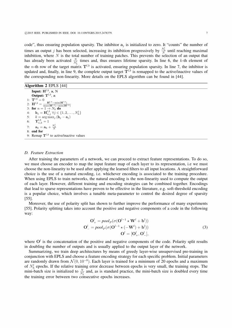
c⃝2015 IEEE. PUBLISHED IN IEEE. DOI: 10.1109/TGRS.2015.2478379. 7
code”, thus ensuring population sparsity. The inhibitor aj is initialized to zero. It “counts” the number oftimes an output j has been selected, increasing its inhibition progressively by N l
hN until reaching maximal
inhibition, where N is the total number of training patches. This prevents the selection of an output thathas already been activated N
N lh
times and, thus ensures lifetime sparsity. In line 6, the k-th element ofthe n-th row of the target matrix Tl,b is activated, ensuring population sparsity. In line 7, the inhibitor isupdated and, finally, in line 9, the complete output target Tl,b is remapped to the active/inactive values ofthe corresponding non-linearity. More details on the EPLS algorithm can be found in [44].
Algorithm 2 EPLS [44]Input: Hl,b, a, NOutput: Tl,b, a
1: Tl,b = 02: Hl,b = Hl,b−min(Hl,b)
max(Hl,b)−min(Hl,b)3: for n = 1→ Nb do4: hj = Hl,b
n,j ∀j ∈ {1, 2, . . . , N lh}
5: k = argmaxj (hj − aj)6: Tl,b
n,k = 1
7: ak = ak + N lh
N8: end for9: Remap Tl,b to active/inactive values
D. Feature ExtractionAfter training the parameters of a network, we can proceed to extract feature representations. To do so,
we must choose an encoder to map the input feature map of each layer to its representation, i.e we mustchoose the non-linearity to be used after applying the learned filters to all input locations. A straightforwardchoice is the use of a natural encoding, i.e. whichever encoding is associated to the training procedure.When using EPLS to train networks, the natural encoding is the non-linearity used to compute the outputof each layer. However, different training and encoding strategies can be combined together. Encodingsthat lead to sparse representations have proven to be effective in the literature, e.g. soft-threshold encodingis a popular choice, which involves a tunable meta-parameter to control the desired degree of sparsity[55].
Moreover, the use of polarity split has shown to further improve the performance of many experiments[55]. Polarity splitting takes into account the positive and negative components of a code in the followingway:
Ol+ = poolP (σ(O
l−1 ⋆Wl + bl))
Ol− = poolP (σ(O
l−1 ⋆ (−Wl) + bl))
Ol = [Ol+,O
l−],
(3)
where Ol is the concatenation of the positive and negative components of the code. Polarity split resultsin doubling the number of outputs and is usually applied to the output layer of the network.
Summarizing, we train deep architectures by means of greedy layer-wise unsupervised pre-training inconjunction with EPLS and choose a feature encoding strategy for each specific problem. Initial parametersare randomly drawn from N (0, 10−8). Each layer is trained for a minimum of 20 epochs and a maximumof N l
h epochs. If the relative training error decrease between epochs is very small, the training stops. Themini-batch size is initialized to N
N lh
and, as is standard practice, the mini-batch size is doubled every timethe training error between two consecutive epochs increases.
c⃝2015 IEEE. PUBLISHED IN IEEE. DOI: 10.1109/TGRS.2015.2478379. 8
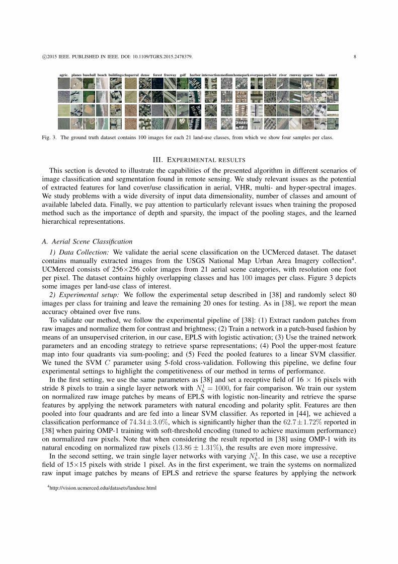
agric. planes baseball beach buildingschaparral dense forest freeway golf harbor intersectionmediumhomeparkoverpasspark-lot river runway sparse tanks court
Fig. 3. The ground truth dataset contains 100 images for each 21 land-use classes, from which we show four samples per class.
III. EXPERIMENTAL RESULTS
This section is devoted to illustrate the capabilities of the presented algorithm in different scenarios ofimage classification and segmentation found in remote sensing. We study relevant issues as the potentialof extracted features for land cover/use classification in aerial, VHR, multi- and hyper-spectral images.We study problems with a wide diversity of input data dimensionality, number of classes and amount ofavailable labeled data. Finally, we pay attention to particularly relevant issues when training the proposedmethod such as the importance of depth and sparsity, the impact of the pooling stages, and the learnedhierarchical representations.
A. Aerial Scene Classification1) Data Collection: We validate the aerial scene classification on the UCMerced dataset. The dataset
contains manually extracted images from the USGS National Map Urban Area Imagery collection4.UCMerced consists of 256×256 color images from 21 aerial scene categories, with resolution one footper pixel. The dataset contains highly overlapping classes and has 100 images per class. Figure 3 depictssome images per land-use class of interest.
2) Experimental setup: We follow the experimental setup described in [38] and randomly select 80images per class for training and leave the remaining 20 ones for testing. As in [38], we report the meanaccuracy obtained over five runs.
To validate our method, we follow the experimental pipeline of [38]: (1) Extract random patches fromraw images and normalize them for contrast and brightness; (2) Train a network in a patch-based fashion bymeans of an unsupervised criterion, in our case, EPLS with logistic activation; (3) Use the trained networkparameters and an encoding strategy to retrieve sparse representations; (4) Pool the upper-most featuremap into four quadrants via sum-pooling; and (5) Feed the pooled features to a linear SVM classifier.We tuned the SVM C parameter using 5-fold cross-validation. Following this pipeline, we define fourexperimental settings to highlight the competitiveness of our method in terms of performance.
In the first setting, we use the same parameters as [38] and set a receptive field of 16 × 16 pixels withstride 8 pixels to train a single layer network with N1
h = 1000, for fair comparison. We train our systemon normalized raw image patches by means of EPLS with logistic non-linearity and retrieve the sparsefeatures by applying the network parameters with natural encoding and polarity split. Features are thenpooled into four quadrants and are fed into a linear SVM classifier. As reported in [44], we achieved aclassification performance of 74.34±3.0%, which is significantly higher than the 62.7±1.72% reported in[38] when pairing OMP-1 training with soft-threshold encoding (tuned to achieve maximum performance)on normalized raw pixels. Note that when considering the result reported in [38] using OMP-1 with itsnatural encoding on normalized raw pixels (13.86± 1.31%), the results are even more impressive.
In the second setting, we train single layer networks with varying N1h . In this case, we use a receptive
field of 15×15 pixels with stride 1 pixel. As in the first experiment, we train the systems on normalizedraw input image patches by means of EPLS and retrieve the sparse features by applying the network
4http://vision.ucmerced.edu/datasets/landuse.html
c⃝2015 IEEE. PUBLISHED IN IEEE. DOI: 10.1109/TGRS.2015.2478379. 9
100 200 300 400 500 600 700 800 900 100068
70
72
74
76
78
80
82
84
86Accuracy
(%)
Number of outputs N lh
Our method − single layerOur method − 2 layersOur method − 3 layersCheriyadat
40 50 60 70 80 90 10040
50
60
70
80
90
100
OMP−1 accuracy (%)
EPLS
acc
urac
y (%
)
single layer2 layers3 layers
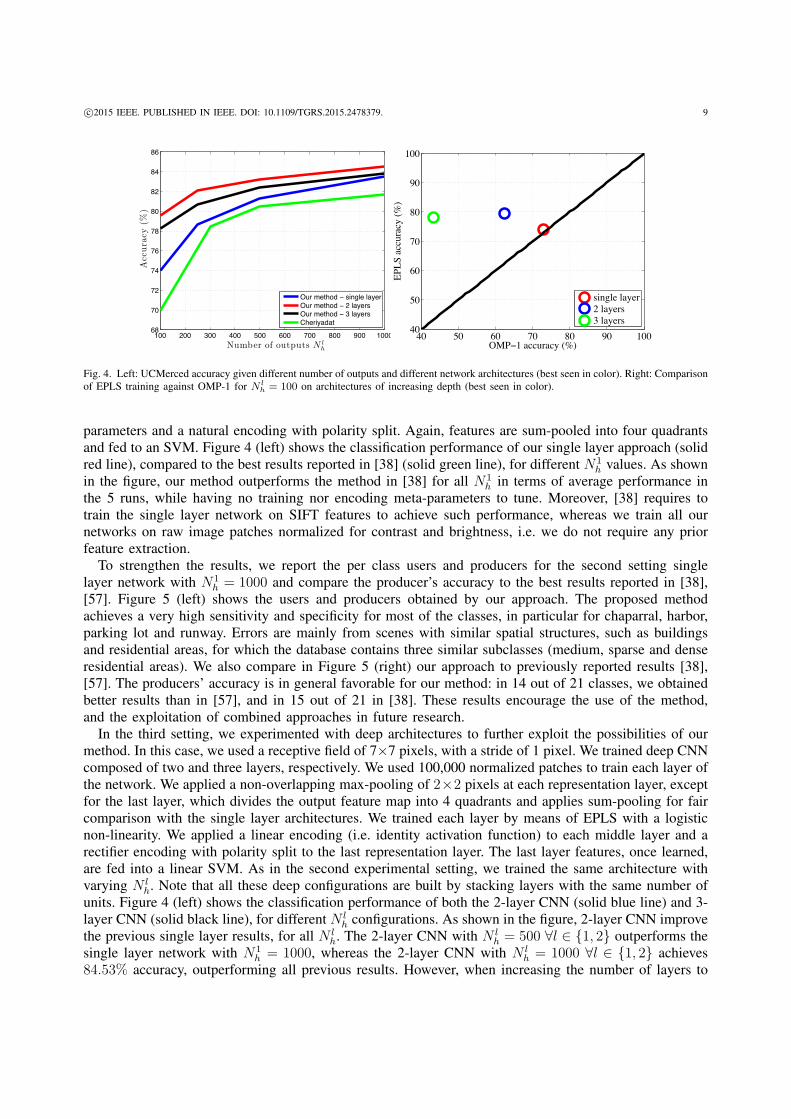
Fig. 4. Left: UCMerced accuracy given different number of outputs and different network architectures (best seen in color). Right: Comparisonof EPLS training against OMP-1 for N l
h = 100 on architectures of increasing depth (best seen in color).
parameters and a natural encoding with polarity split. Again, features are sum-pooled into four quadrantsand fed to an SVM. Figure 4 (left) shows the classification performance of our single layer approach (solidred line), compared to the best results reported in [38] (solid green line), for different N1
h values. As shownin the figure, our method outperforms the method in [38] for all N1
h in terms of average performance inthe 5 runs, while having no training nor encoding meta-parameters to tune. Moreover, [38] requires totrain the single layer network on SIFT features to achieve such performance, whereas we train all ournetworks on raw image patches normalized for contrast and brightness, i.e. we do not require any priorfeature extraction.
To strengthen the results, we report the per class users and producers for the second setting singlelayer network with N1
h = 1000 and compare the producer’s accuracy to the best results reported in [38],[57]. Figure 5 (left) shows the users and producers obtained by our approach. The proposed methodachieves a very high sensitivity and specificity for most of the classes, in particular for chaparral, harbor,parking lot and runway. Errors are mainly from scenes with similar spatial structures, such as buildingsand residential areas, for which the database contains three similar subclasses (medium, sparse and denseresidential areas). We also compare in Figure 5 (right) our approach to previously reported results [38],[57]. The producers’ accuracy is in general favorable for our method: in 14 out of 21 classes, we obtainedbetter results than in [57], and in 15 out of 21 in [38]. These results encourage the use of the method,and the exploitation of combined approaches in future research.
In the third setting, we experimented with deep architectures to further exploit the possibilities of ourmethod. In this case, we used a receptive field of 7×7 pixels, with a stride of 1 pixel. We trained deep CNNcomposed of two and three layers, respectively. We used 100,000 normalized patches to train each layer ofthe network. We applied a non-overlapping max-pooling of 2×2 pixels at each representation layer, exceptfor the last layer, which divides the output feature map into 4 quadrants and applies sum-pooling for faircomparison with the single layer architectures. We trained each layer by means of EPLS with a logisticnon-linearity. We applied a linear encoding (i.e. identity activation function) to each middle layer and arectifier encoding with polarity split to the last representation layer. The last layer features, once learned,are fed into a linear SVM. As in the second experimental setting, we trained the same architecture withvarying N l
h. Note that all these deep configurations are built by stacking layers with the same number ofunits. Figure 4 (left) shows the classification performance of both the 2-layer CNN (solid blue line) and 3-layer CNN (solid black line), for different N l
h configurations. As shown in the figure, 2-layer CNN improvethe previous single layer results, for all N l
h. The 2-layer CNN with N lh = 500 ∀l ∈ {1, 2} outperforms the
single layer network with N1h = 1000, whereas the 2-layer CNN with N l
h = 1000 ∀l ∈ {1, 2} achieves84.53% accuracy, outperforming all previous results. However, when increasing the number of layers to

c⃝2015 IEEE. PUBLISHED IN IEEE. DOI: 10.1109/TGRS.2015.2478379. 10
AgriculturalAirplane
BaseballdiamondBeach
BuildingsChaparral
DenseresidentialForest
FreewayGolfcourse
HarborIntersection
MediumresidentialMobilehomepark
OverpassParkinglot
RiverRunway
SparseresidentialStoragetanksTenniscourt
Classes
Per c
lass
use
rs/p
rodu
cers
[%]
UsersProducers
50 60 70 80 90 10050
55
60
65
70
75
80
85
90
95
100
Others
Our
met
hod
Producers’ accuracy [%]
Cheridayat, 2014Yang, 2010
Fig. 5. Results in UCMerced experiment. Left: users and producers per class obtained with the proposed method. Right: comparison of ourmethod to previous works in the literature in terms of producers (accuracy per class) [38], [57]. We took the results for the best algorithmsin both [57] (their Figure 8, ‘color’ model) and [38] (his Fig. 13, dense SIFT descriptors) (best seen in color).
3, the accuracy starts dropping. We argue whether the UCMerced dataset could benefit from a higherlevel of abstraction in its feature representation, given the (high) amount of texture present in its images.Even if it could benefit from the higher abstraction, the layer-wise pre-training might be too greedy and afine-tuning step might be required to achieve better performance as we increase the depth of the network.Furthermore, the receptive field size could be appropriately tuned to improve the results; note that theimage region considered in the 3rd layer is much bigger than the ones considered by the 1st and 2ndlayers. Finally, it is worth noticing that as we increase the number of layers, the number of parametersincreases dramatically and the model becomes more prone to overfit.
After highlighting the impact of stacking hierarchical (deep) representations, we designed an experimentto assess the importance of sparsity to achieve good representations. In order to highlight the relevance oflifetime sparsity in deep scenarios, we used OMP-1 as a substitute of EPLS and reproduced the experimentsin Figure 4 (left) for N l
h = 100. Figure 4 (right) reports the obtained results. In the case of the single layernetwork (red circle), EPLS achieves slightly better results than OMP-1. However, as shown in the Figure,OMP-1 seems not to be able to take advantage of depth. When adding a second layer to the architecture(blue circle), OMP-1 experiences a performance drop of 10.38%, whereas ELPS improves its performanceby 5.52%. When adding a third layer to the architecture (green circle), both OMP-1 and EPLS decreasetheir performances. OMP-1’s performance drop is particularly dramatic (from 72.90% in the single layerarchitecture to 43.14% in the 3-layer architecture). We argue this dramatic performance drop is related tothe OMP-1’s lack of lifetime sparsity, which makes the algorithm suffer from dead outputs (i.e. outputs thatnever activate). While increasing the network’s depth, the dead outputs’ effect becomes more significantand impacts the performance of the method. Therefore, enforcing lifetime sparsity is crucial for EPLS toachieve good performance.
B. Very high resolution (VHR) image classificationVery high spatial resolution (VHR) has been one of the major achievements of satellite imagery of
the last decades. Sensors providing sub-metric resolution have been developed and satellites such asQuickBird, GeoEye-1 or WorldView-3 have been or are about to be launched. These sensors provideimages that are unique in terms of spatial detail and open a wide range of challenges for geospatialinformation processing. This application example studies how to extract discriminative features fromVHR imagery in an unsupervised way via the deep CNN proposed here.
1) Data Collection: To do the experiments, we used two VHR images acquired with the Quickbirdinstrument. The satellite data were obtained from Quickbird II, which employs a four-band sensor with

c⃝2015 IEEE. PUBLISHED IN IEEE. DOI: 10.1109/TGRS.2015.2478379. 11
2.4-m spatial resolution for blue, green, red and near-infrared spectral wavelengths and a 0.6-m resolu-tion panchromatic band ( c⃝2008 Digitalglobe, all rights reserved). Images acquisitions were obtained tocoincide with seasonal base flow conditions and field surveys during late summer or early fall periods.Each image was georeferenced using field-collected ground control points that yielded an average rootmean square geolocation error of less than 1.5 m.
The images were acquired over Nayak-Middle Fork (1659×1331×4) of the Flathead River in the Nyackflood plain bordering Glacier National Park, Montana, and the Kol flood plain (1617×1660×4), during2008. Both images have been widely used to study and characterize the physical complexity of NorthPacific Rim rivers to assist wild salmon conservation. The labeled land used classes are actually relatedto such properties: shallow shore, parafluvial, and orthofluvial salmon habitats types [58], [59].
Fig. 6. RGB composition of the two VHR images considered for classification: ‘Nayak - Middle Fork’ (left) and ‘Kol’ (right).
2) Experimental setup: The setting involves an independent feature extraction and classification perimage, which is a standard scenario in remote sensing image classification. The aim of the experimentis to assess in two independent images the capabilities of CNN architectures to extract useful features tocapture spectral-spatial structure for habitat classification. The experiments are conducted for a varyingnumber of layers and number of training examples. For the single layer architecture the receptive field isset to 5× 5 pixels, while for deep architectures the receptive field is set to 3× 3 pixels. In all cases, eachlayer has 200 outputs, i.e. N l
h = 200 ∀l. CNN are trained in a layer-wise fashion by means of EPLS withlogistic non-linearity as unsupervised criterion. A non-overlapping max-pooling of size 2 × 2 pixels isapplied to the output of the hidden layers, except for the last representation layer, which does not performany pooling operation. We choose a natural encoding without polarity split to map the input of each layerto its output representation. The output of the last layer is fed to a 1-Nearest Neighbor (1-NN) classifierwith Euclidean distance.
Figure 7 shows the classification results in terms of overall accuracy (OA) and kappa statistic for thetwo VHR images, as a function of the number of training samples ({0.5%, 1%, 2.5%, 5%, 10%}) and thenumber of layers (1–6) considered in the model. Three main conclusions are drawn from the experiments:1) results are improved with more training samples, as expected; 2) non-linear feature extraction (bothkPCA and CNN) outperform the linear PCA; and 3) the deeper the network, the better the results. Weobserved an average gain with a deep CNN of about +10% for the Nayak image and of +20% for the Kolimage in terms of kappa statistic. Results saturate for 6 layers and for more than 5% of training samples(this issue has been also observed in the hyper-spectral image classification problem in the followingsections).
C. Multispectral image classificationThis experiment is concerned with the challenging problem of cloud screening using multispectral
images.

c⃝2015 IEEE. PUBLISHED IN IEEE. DOI: 10.1109/TGRS.2015.2478379. 12
PCA kPCA 1 2 3 4 5 60
20
40
60
80
100
Layers
Ove
rall
accu
racy
, OA
[%]
Nayak − Middle Fork
0.5%1%2.5%5%10%
PCA kPCA 1 2 3 4 5 60
0.2
0.4
0.6
0.8
1
Layers
Kap
pa
Nayak − Middle Fork
0.5%1%2.5%5%10%
PCA kPCA 1 2 3 4 5 60
20
40
60
80
100
Layers
Ove
rall
accu
racy
, OA
[%]
Kol
0.5%1%2.5%5%10%
PCA kPCA 1 2 3 4 5 60
0.2
0.4
0.6
0.8
1
Layers
Kap
pa
Kol
0.5%1%2.5%5%10%
Fig. 7. Classification results (OA and kappa statistic) in the form of the average ± standard deviation bars over 10 realizations of theclassification experiment in two VHR images, as a function of the number of training samples and CNN depth.
1) Data Collection: To do the experiments, we used seven images acquired with the Medium ResolutionImaging Spectrometer (MERIS) instrument on-board the Environmental Satellite (ENVISAT). In particular,we used images acquired over Abracos (2004), Ascension Island (2005), Azores (2004), Barcelona (2006),Capo Verde (2005), Longyearbyen (2006) and Mongu (2003). All images are of size 321×490, andall 16 channels were used for the feature extraction. The selected images represent different scenariosextremely useful to validate the performance of the method, including different landscapes; soils coveredby vegetation or bare; and critical cases given the special characteristics of the induced problems: ice andsnow. Note that the images cover different characteristics as well: geographic location, date and season,type of cloud, and surface types.
2) Experimental setup: Most approaches to tackle the problem of cloud screening rely on neuralnetworks or kernel machines trained with supervision: they assume the existence of a labeled trainingdataset that serves to tune model parameters [60]–[64]. In our approach, more in line of the unsupervisedclustering approach presented in [65], we alternatively test the scheme of unsupervised deep featureextraction followed by a simple 1-NN classifier with Euclidean distance. The main goal is to attain a fullyunsupervised, meta-parameter free scheme.
The proposed experimental setup allows to assess the expressive power of the extracted features in avery consistent way. Essentially, the scheme performs an image-fold cross-validation through both featuresand samples. Classification of pixels in an image needs to learn the features for that particular image: inour setting, we apply the deep CNN learned from other images without any re-training of the weights orfilters. For classification, the inferred features are fed to the 1-NN classifier. The deep architecture wasdesigned such that all layers have the same number of outputs, i.e. N l
h = 120 ∀l. We used a receptive field

c⃝2015 IEEE. PUBLISHED IN IEEE. DOI: 10.1109/TGRS.2015.2478379. 13
of size 5× 5 pixels. We trained the CNN layer-wise by means of EPLS with logistic activation function5,and incorporated a max-pooling operator of size 2 × 2 after each intermediate representation. We didnot perform any kind of pooling after the last representation layer. We applied natural encoding withoutpolarity split to extract the features of each layer. We compare the feature extraction performed by theproposed CNN to the feature extraction performed by PCA and kPCA. For the sake of a fair comparison,we extracted a fixed number of features in all cases: we set a number of features Nf = 120 for both PCAand kPCA and used N l
h = 120 ∀l in the CNN case (l = 2 exhibited the best results). For kPCA, we usedan RBF kernel and set the lengthscale parameter to the average distance between all training samples, asa reasonable estimate (note that the feature extraction is unsupervised, so there are no labels at this stageto tune kernel parameters). We fed the extracted features to a 1-NN classifier.
3) Expressive and discriminative power: Given the difficulty of obtaining labeled training samplesin this problem, we simulate the expressive power of the extracted features using different numbers oftraining pixels for classification. Figure 8 shows the evolution of two classification scores with the numberof training samples: the overall accuracy (OA) and the estimated Cohen’s kappa statistic, κ. Results showthat both measures are consistent (convergence with the number of samples), and no big differences areobserved between OA and κ so the classifications are, in principle, unbiased. We noted that in general theproposed CNN performs better than the other feature extractors, especially when few training samples areused for classification. This suggests that the extracted features are more discriminative and rich, whichcan be compensated with the information conveyed by using more labeled examples. Interestingly, wefound that tuning the kernel parameter for kPCA becomes very complex; even though we here show theresults for the standard ‘rule of thumb’ of setting the lengthscale to the average distance between points,we tried different other alternatives but still the simple spectral approach (no feature extraction) yieldedbetter results than kPCA.
101 10250
60
70
80
90
100
# Training samples
Ove
rall
accu
racy
, OA
[%]
SpectralKPCACNN
101 1020.1
0.2
0.3
0.4
0.5
0.6
# Training samples
stat
istic
SpectralKPCACNN
Fig. 8. Classification results (mean and standard deviation) over the seven MS images used as a function of the number of training samples.
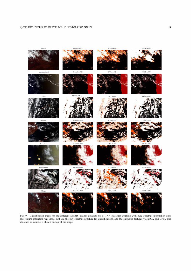
4) Visual Validation of the results: Figure 9 shows the classification maps obtained with a 1-NNclassifier using the spectral information only, and on top of the extracted features using kPCA andCNN. In terms of numerical results, CNN clearly outperforms the rest of approaches. In all cases, weobserved an average gain between 5-30% in κ statistic (see e.g. outstanding results on ‘Abracos’, ‘Mongu’or ‘Longyearbyen’ scenes). It should be also noted that in some particular cases (e.g. ‘Azores’, ‘CapoVerde’, and ‘Longyearbyen’) CNN does only significantly improve the results over kPCA, not the spectralapproach, which is probably due to the low efficiency in extracting spatially relevant features over areashighly affected by clouds over snowy mountains (that lead to non-interesting features), sunglint (as in theeast part of Capo Verde) or very easy images as in the case of compact clouds over sea (Azores scene).In some other cases with similar conditions (e.g. sunglint in Ascension island) the gain obtained bythe proposed CNN is noticeable (+6% over spectral features and +12% over kPCA), especially because
5We also tried with a linear activation function but the extracted features were less performing.
c⃝2015 IEEE. PUBLISHED IN IEEE. DOI: 10.1109/TGRS.2015.2478379. 14
Abracos Spectral, κ=0.57 KPCA, κ=0.50 NNET, κ=0.81
Ascension Island Spectral, κ=0.26 KPCA, κ=0.21 NNET, κ=0.33
AzoresSpectral, κ=0.93 KPCA, κ=0.83 NNET, κ=0.94
Barcelona Spectral, κ=0.66 KPCA, κ=0.58 NNET, κ=0.72
Capo Verde Spectral, κ=0.64 KPCA, κ=0.53 NNET, κ=0.65
Longyearbyen Spectral, κ=0.73 KPCA, κ=0.51 NNET, κ=0.73
Mongu Spectral, κ=0.40 KPCA, κ=0.35 NNET, κ=0.58
Fig. 9. Classification maps for the different MERIS images obtained by a 1-NN classifier working with pure spectral information only(no feature extraction was done, just use the raw spectral signature for classification), and the extracted features via kPCA and CNN. Theobtained κ statistic is shown on top of the maps.
c⃝2015 IEEE. PUBLISHED IN IEEE. DOI: 10.1109/TGRS.2015.2478379. 15
of the high rate of positive detections in the part of the scene not affected by the sunglint. Anotherinteresting case of study is the Barcelona image in which similar maps are obtained by all methods;nevertheless CNN yields a lower false alarm rate in compact structures (southern and northern big clouds)thus demonstrating that the spatial-spectral information has been very well captured. A more dramaticgain showing this particularity of the method is shown in the Abracos and Mongu scenes, where +30%and 18-23% average gain is attained by CNN, respectively, thanks to a reduced false alarm rate in cloudsover flat landscapes.
D. Hyperspectral image classificationThis section illustrates the performance of the proposed method in a challenging hyper-spectral image
classification problem. We compare the features extracted by CNN of varying depth to the ones extractedby PCA and kPCA in terms of expressive power, classification accuracy, and robustness to the numberof labeled examples.
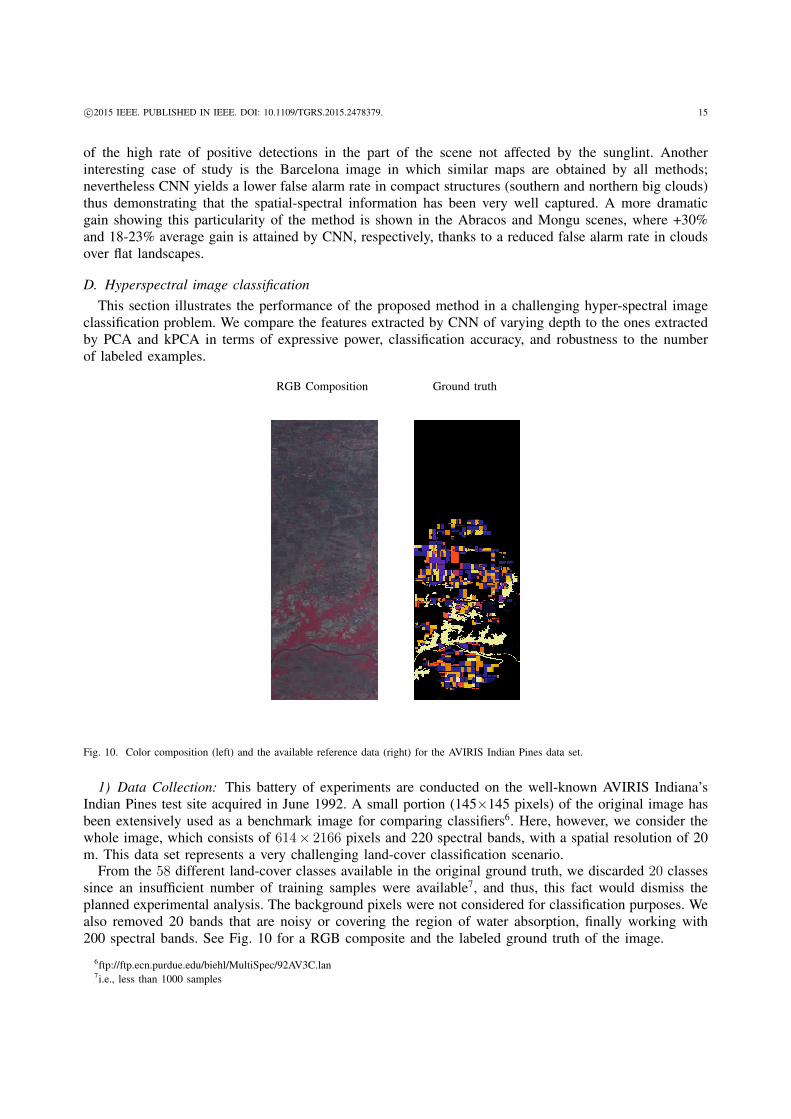
RGB Composition Ground truth
Fig. 10. Color composition (left) and the available reference data (right) for the AVIRIS Indian Pines data set.
1) Data Collection: This battery of experiments are conducted on the well-known AVIRIS Indiana’sIndian Pines test site acquired in June 1992. A small portion (145×145 pixels) of the original image hasbeen extensively used as a benchmark image for comparing classifiers6. Here, however, we consider thewhole image, which consists of 614× 2166 pixels and 220 spectral bands, with a spatial resolution of 20m. This data set represents a very challenging land-cover classification scenario.
From the 58 different land-cover classes available in the original ground truth, we discarded 20 classessince an insufficient number of training samples were available7, and thus, this fact would dismiss theplanned experimental analysis. The background pixels were not considered for classification purposes. Wealso removed 20 bands that are noisy or covering the region of water absorption, finally working with200 spectral bands. See Fig. 10 for a RGB composite and the labeled ground truth of the image.
6ftp://ftp.ecn.purdue.edu/biehl/MultiSpec/92AV3C.lan7i.e., less than 1000 samples
c⃝2015 IEEE. PUBLISHED IN IEEE. DOI: 10.1109/TGRS.2015.2478379. 16
(a) (b)
5 10 20 50 100 2000
0.1
0.2
0.3
0.4
0.5
0.6
0.7
0.8
0.9
1
Number of features
κ
PCA, 1x1PCA, 3x3PCA, 5x5KPCA, 1x1KPCA, 3x3KPCA, 5x5NNET, 1x1NNET, 3x3NNET, 5x5
2 3 4 5 6 70
0.1
0.2
0.3
0.4
0.5
0.6
0.7
0.8
0.9
1
Number of layers
κ
No max−poolingMax−pooling
(c) (d)
0 0.1 0.2 0.3 0.4 0.50.2
0.3
0.4
0.5
0.6
0.7
0.8
0.9
1
Rate of training samples/class
κ
L2L3L4L5L6L7
100 1100 2100 3100 41000%
2%
4%
6%
8%
10%
12%
14%
16%
18%
20%
Fig. 11. Classification accuracy estimated with the kappa statistic for (a) several numbers of features, spatial extent of the receptive fields(for the single layer network) or the included Gaussian filtered features (for PCA and kPCA) using 30% of data for training; (b) impact of thenumber of layers on the networks with and without pooling stages; (c) for different rates of training samples, {1%, 5%, 10%, 20%, 30%, 50%},with pooling; and (d) percentage of ground truth pixels as a function of labeled region areas (see text for details).
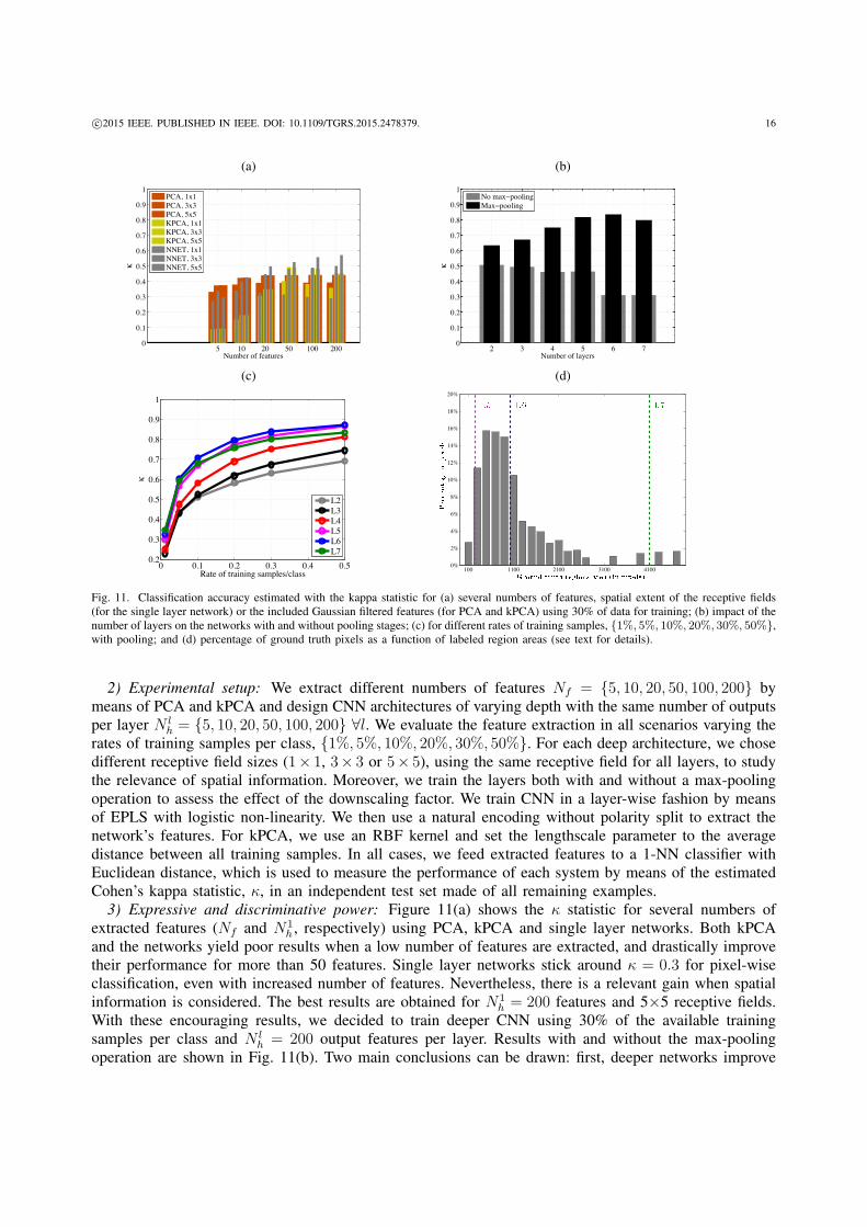
2) Experimental setup: We extract different numbers of features Nf = {5, 10, 20, 50, 100, 200} bymeans of PCA and kPCA and design CNN architectures of varying depth with the same number of outputsper layer N l
h = {5, 10, 20, 50, 100, 200} ∀l. We evaluate the feature extraction in all scenarios varying therates of training samples per class, {1%, 5%, 10%, 20%, 30%, 50%}. For each deep architecture, we chosedifferent receptive field sizes (1× 1, 3× 3 or 5× 5), using the same receptive field for all layers, to studythe relevance of spatial information. Moreover, we train the layers both with and without a max-poolingoperation to assess the effect of the downscaling factor. We train CNN in a layer-wise fashion by meansof EPLS with logistic non-linearity. We then use a natural encoding without polarity split to extract thenetwork’s features. For kPCA, we use an RBF kernel and set the lengthscale parameter to the averagedistance between all training samples. In all cases, we feed extracted features to a 1-NN classifier withEuclidean distance, which is used to measure the performance of each system by means of the estimatedCohen’s kappa statistic, κ, in an independent test set made of all remaining examples.
3) Expressive and discriminative power: Figure 11(a) shows the κ statistic for several numbers ofextracted features (Nf and N1
h , respectively) using PCA, kPCA and single layer networks. Both kPCAand the networks yield poor results when a low number of features are extracted, and drastically improvetheir performance for more than 50 features. Single layer networks stick around κ = 0.3 for pixel-wiseclassification, even with increased number of features. Nevertheless, there is a relevant gain when spatialinformation is considered. The best results are obtained for N1
h = 200 features and 5×5 receptive fields.With these encouraging results, we decided to train deeper CNN using 30% of the available trainingsamples per class and N l
h = 200 output features per layer. Results with and without the max-poolingoperation are shown in Fig. 11(b). Two main conclusions can be drawn: first, deeper networks improve

c⃝2015 IEEE. PUBLISHED IN IEEE. DOI: 10.1109/TGRS.2015.2478379. 17
the accuracy enormously (the 6-layer network reaches the highest accuracy of κ = 0.84), and second,including the max-pooling operation after each intermediate layer revealed to be extremely beneficial. Weshould stress that this result clearly outperforms the previously reported state-of-the-art result (κ = 0.75)obtained with a SVM on the same experimental setting [66].
4) Robustness w.r.t. number of training labels: Another question to be addressed is the robustness ofthe features in terms of number of training examples. Figure 11(c) highlights that using a few supervisedsamples to train a deep CNN can provide better results than using far more supervised samples to traina single layer one. Note, for instance, that the 6-layer network using 5% samples/class outperforms thebest single layer network using 30% of the samples/class.
5) Need and limitation of spatial pooling: Special attention should be devoted to the 7-layer network.In this case, the accuracy decreases since the potential contribution of an additional layer is stronglycounterbalanced by the heavily reduced spatial resolution of the additional max-pooling. The topmostlayer has no max-pooling since it is used as output. To corroborate this explanation, we created thehistogram in Figure 11(d), which shows the percentage of ground truth pixels as a function of labeledregion areas. As it can also be seen in Figure 10(right), the labeled regions are mainly rectangular withan average area around 500 pixels. Vertical lines in Figure 11(d) show the theoretical spatial resolutionin the case the output layer is resized using a nearest neighbor interpolation. As it can be observed, whenusing 7 layers (L7, green), the resolution is too low to capture regions smaller than 4096 pixels (64×64).It has to be noted that we perform the upscaling of the output layer by means of a bilinear interpolation;this explains why, despite the lower spatial resolution, the result using 6 layers is still superior to the onewith 5 layers.
6) Learned features: An important aspect of the proposed deep architectures lies in the fact that theytypically give rise to compact hierarchical representations. The best three features extracted by the networksaccording to the mutual information with labels are depicted in Fig. 12 for a subset of the whole image.It is worth stressing that the deeper we go, the more complicated and abstract features we retrieve, exceptfor the seventh layer that provides spatially over-regularized features due to the downscaling impact ofthe max-pooling stages. Interestingly, it is also observed that, the deeper structures we use, the higherspatial decorrelation of the best features we obtain.
Fig. 12. Best three features (in rows) according to the mutual information with the labels for the outputs of the different layers 1st to 7th(in columns) for a subregion of the whole image.
IV. CONCLUSIONS
We introduced deep learning for unsupervised feature extraction of remote sensing images. The proposedapproach consists of using a convolutional neural network trained with an unsupervised algorithm that
c⃝2015 IEEE. PUBLISHED IN IEEE. DOI: 10.1109/TGRS.2015.2478379. 18
promotes two types of feature sparsity: population and lifetime sparsity. The algorithm trains the networkparameters to learn hierarchical sparse representations of the input images that can be fed to a simpleclassifier. We should stress that the unsupervised learning of features is computationally very efficient,having a computational cost equal to OMP-1 while clearly outperforming it. Furthermore, the featureextraction stage is meta-parameter free, whereas the classification stage involves either one or zero free-parameters. Note that we applied the linear SVM classifier with one tunable parameter in experimentSection III-A for fair comparison with the state-of-the-art. We trained deep convolutional networks in agreedy layer-wise fashion and performed experiments to analyze the influence of depth and pooling ofsuch networks on a wide variety of remote sensing images of different spatial and spectral resolutions,from multi- and hyper-spectral images, to very high geometrical resolution problems.
Results reveal that the trained networks are very effective at encoding spatio-spectral information ofthe images. Experiments showed that (1) including spatial information is essential in order to avoid poorperformance in single layer networks; (2) combining high numbers of output features and max-poolingsteps in deep architectures is crucial to achieve excellent results; and (3) adding new layers to the deeparchitecture improves the classification score substantially, until the repeated max-pooling steps heavilyreduce the features spatial resolution and/or the number of parameters becomes too large, thus inducinga form of overfitting.
Further work is tied to assessing generalization of the encoded features in multi-temporal and multi-angular image settings, as well as to explore the suitability of the extracted features to perform biophysicalparameter retrieval. Moreover, it would be interesting to analyze the feature’s degree of sparsity requiredat each layer to achieve a discriminative system w.r.t. the classifier and adapt the EPLS to train towards thedesired degree of sparsity at each layer. Furthermore, to avoid overfitting while increasing the number ofparameters, algorithms such as drop-out [67] could be tested. Finally, since greedy layer-wise pre-traininghas shown to require a supervised finetuning step to make the network parameters more task specific,and thus improve the network’s performance, further investigation should be devoted to find alternativesto train deep networks without relying on large amounts of labeled data, or even the more challengingtask of being able to cope with completely unsupervised settings. Given the large amounts of processingrequired, algorithms should aim at remaining computationally efficient, especially at training time.
ACKNOWLEDGMENTS
The authors wish to thank Antonio Plaza from the University of Extremadura, Spain, for kindlyproviding the AVIRIS dataset, and Prof. Diane Whited at the University of Montana for the VHR imageryused in some experiments of this paper.
REFERENCES
[1] S. Liang, Quantitative Remote Sensing of Land Surfaces. New York: John Wiley & Sons, 2004.[2] T. M. Lillesand, R. W. Kiefer, and J. Chipman, Remote Sensing and Image Interpretation. New York: John Wiley & Sons, 2008.[3] G. Shaw and D. Manolakis, “Signal processing for hyperspectral image exploitation,” IEEE Signal Proc. Magazine, vol. 50, pp. 12–16,
Jan 2002.[4] G. Camps-Valls, D. Tuia, L. Bruzzone, and J. Atli Benediktsson, “Advances in hyperspectral image classification: Earth monitoring
with statistical learning methods,” Signal Processing Magazine, IEEE, vol. 31, no. 1, pp. 45–54, Jan 2014.[5] G. Camps-Valls, D. Tuia, L. Gomez-Chova, S. Jimenez, and J. Malo, Eds., Remote Sensing Image Processing. LaPorte, CO, USA:
Morgan & Claypool Publishers, Sept 2011.[6] R. Willett, M. Duarte, M. Davenport, and R. Baraniuk, “Sparsity and structure in hyperspectral imaging : Sensing, reconstruction, and
target detection,” Signal Processing Magazine, IEEE, vol. 31, no. 1, pp. 116–126, Jan 2014.[7] W.-K. Ma, J. Bioucas-Dias, T.-H. Chan, N. Gillis, P. Gader, A. Plaza, A. Ambikapathi, and C.-Y. Chi, “A signal processing perspective
on hyperspectral unmixing: Insights from remote sensing,” Signal Processing Magazine, IEEE, vol. 31, no. 1, pp. 67–81, Jan 2014.[8] G. Arce, D. Brady, L. Carin, H. Arguello, and D. Kittle, “Compressive coded aperture spectral imaging: An introduction,” Signal
Processing Magazine, IEEE, vol. 31, no. 1, pp. 105–115, Jan 2014.[9] D. Roy, M. Wulder, T. Loveland, W. C.E., R. Allen, M. Anderson, D. Helder, J. Irons, D. Johnson, R. Kennedy, T. Scambos, C. Schaaf,
J. Schott, Y. Sheng, E. Vermote, A. Belward, R. Bindschadler, W. Cohen, F. Gao, J. Hipple, P. Hostert, J. Huntington, C. Justice,A. Kilic, V. Kovalskyy, Z. Lee, L. Lymburner, J. Masek, J. McCorkel, Y. Shuai, R. Trezza, J. Vogelmann, R. Wynne, and Z. Zhu,“Landsat-8: Science and product vision for terrestrial global change research,” Remote Sensing of Environment, vol. 145, no. 0, pp.154 – 172, 2014.

c⃝2015 IEEE. PUBLISHED IN IEEE. DOI: 10.1109/TGRS.2015.2478379. 19
[10] N. Longbotham, F. Pacifici, B. Baugh, and G. Camps-Valls, “Prelaunch assessment of worldview-3 information content,” in Whispers2014, Lausanne, Switzerland, 2014, pp. 479–486.
[11] M. Drusch, U. Del Bello, S. Carlier, O. Colin, V. Fernandez, F. Gascon, B. Hoersch, C. Isola, P. Laberinti, P. Martimort, A. Meygret,F. Spoto, O. Sy, F. Marchese, and P. Bargellini, “Sentinel-2: ESA’s Optical High-Resolution Mission for GMES Operational Services,”Remote Sensing of Environment, vol. 120, pp. 25–36, 2012.
[12] C. Donlon, B. Berruti, A. Buongiorno, M.-H. Ferreira, P. Femenias, J. Frerick, P. Goryl, U. Klein, H. Laur, C. Mavrocordatos, J. Nieke,H. Rebhan, B. Seitz, J. Stroede, and R. Sciarra, “The Global Monitoring for Environment and Security (GMES) Sentinel-3 mission,”Remote Sensing of Environment, vol. 120, pp. 37–57, 2012.
[13] T. Stuffler, C. Kaufmann, S. Hofer, K. Farster, G. Schreier, A. Mueller, A. Eckardt, H. Bach, B. Penne, U. Benz, and R. Haydn, “TheEnMAP hyperspectral imager-An advanced optical payload for future applications in Earth observation programmes,” Acta Astronautica,vol. 61, no. 1-6, pp. 115–120, 2007.
[14] D. Roberts, D. Quattrochi, G. Hulley, S. Hook, and R. Green, “Synergies between VSWIR and TIR data for the urban environment: Anevaluation of the potential for the Hyperspectral Infrared Imager (HyspIRI) Decadal Survey mission,” Remote Sensing of Environment,vol. 117, pp. 83–101, 2012.
[15] S. Kraft, U. Del Bello, M. Bouvet, M. Drusch, and J. Moreno, “Flex: Esa’s earth explorer 8 candidate mission,” 2012, pp. 7125–7128.[16] G. Camps-Valls and L. Bruzzone, “Kernel-based methods for hyperspectral image classification,” Geoscience and Remote Sensing,
IEEE Transactions on, vol. 43, no. 6, pp. 1351–1362, June 2005.[17] G. Camps-Valls and L. Bruzzone, Eds., Kernel methods for Remote Sensing Data Analysis. UK: Wiley & Sons, Dec 2009.[18] I. Jolliffe, Principal component analysis. Springer, 2002.[19] J. A. Lee and M. Verleysen, Nonlinear dimensionality reduction. Springer, 2007.[20] C. Bachmann, T. Ainsworth, and R. Fusina, “Improved manifold coordinate representations of large-scale hyperspectral scenes,” IEEE
Trans. Geosci. Remote Sens., vol. 44, no. 10, pp. 2786–2803, 2006.[21] J. Arenas-Garcıa, K. B. Petersen, G. Camps-Valls, and L. K. Hansen, “Kernel multivariate analysis framework for supervised subspace
learning: A tutorial on linear and kernel multivariate methods,” IEEE Sig. Proc. Mag., vol. 30, no. 4, pp. 16–29, 2013.[22] G. E. Hinton and R. R. Salakhutdinov, “Reducing the dimensionality of data with neural networks,” Science, vol. 313, no. 5786, pp.
504–507, July 2006.[23] V. Laparra, G. Camps, and J. Malo, “Iterative gaussianization: from ICA to random rotations,” IEEE Trans. Neur. Nets., vol. 22, no. 4,
pp. 537–549, 2011.[24] A. Baraldi and F. Parmiggiani, “A neural network for unsupervised categorization of multivalued input patterns: an application to
satellite image clustering,” IEEE Transactions on Geoscience and Remote Sensing, vol. 33, no. 2, pp. 305–316, Mar 1995.[25] S. Ghosh, L. Bruzzone, S. Patra, F. Bovolo, and A. Ghosh, “A context-sensitive technique for unsupervised change detection based on
hopfield-type neural networks,” IEEE Transactions on Geoscience and Remote Sensing, vol. 45, no. 3, pp. 778–789, March 2007.[26] F. Del Frate, G. Licciardi, and R. Duca, “Autoassociative neural networks for features reduction of hyperspectral data,” in Hyperspectral
Image and Signal Processing: Evolution in Remote Sensing, 2009. WHISPERS ’09. First Workshop on, Aug 2009, pp. 1–4.[27] G. Licciardi, F. Del Frate, and R. Duca, “Feature reduction of hyperspectral data using autoassociative neural networks algorithms,” in
Geoscience and Remote Sensing Symposium,2009 IEEE International,IGARSS 2009, vol. 1, July 2009, pp. I–176–I–179.[28] C. Vaduva, I. Gavat, and M. Datcu, “Deep learning in very high resolution remote sensing image information mining communication
concept,” in Signal Processing Conference (EUSIPCO), 2012 Proceedings of the 20th European, Aug 2012, pp. 2506–2510.[29] V. Mnih and G. Hinton, “Learning to label aerial images from noisy data,” 2012.[30] X. Chen, S. Xiang, C.-L. Liu, and C.-H. Pan, “Vehicle detection in satellite images by hybrid deep convolutional neural networks,”
IEEE Geosci. Remote Sens. Lett., vol. 11, no. 10, pp. 1797–1801, 2014.[31] Y. Chen, Z. Lin, X. Zhao, G. Wang, and Y. Gu, “Deep learning-based classification of hypersepctral data,” IEEE J. Sel. Topics Appl.
Earth Observ., vol. 7, no. 6, pp. 2094–2107, 2014.[32] Z. Wang, N. Nasrabadi, and T. Huang, “Spatial-spectral classification of hyperspectral images using discriminative dictionary designed
by learning vector quantization,” IEEE Trans. Geosc. Rem. Sens., vol. PP, no. 99, pp. 1–15, 2013.[33] S. Yang, H. Jin, M. Wang, Y. Ren, and L. Jiao, “Data-driven compressive sampling and learning sparse coding for hyperspectral image
classification,” IEEE Geosc. Rem. Sens. Lett., vol. 11, no. 2, pp. 479–483, Feb 2014.[34] S. Li, H. Yin, and L. Fang, “Remote sensing image fusion via sparse representations over learned dictionaries,” IEEE Trans. Geosc.
Rem. Sens., vol. 51, no. 9, pp. 4779–4789, Sept 2013.[35] D. Dai and W. Yang, “Satellite image classification via two-layer sparse coding with biased image representation,” IEEE Geosc. Rem.
Sens. Lett., vol. 8, no. 1, pp. 173–176, Jan 2011.[36] I. Rigas, G. Economou, and S. Fotopoulos, “Low-level visual saliency with application on aerial imagery,” IEEE Geosc. Rem. Sens.
Lett., vol. 10, no. 6, pp. 1389–1393, Nov 2013.[37] H. Sun, X. Sun, H. Wang, Y. Li, and X. Li, “Automatic target detection in high-resolution remote sensing images using spatial sparse
coding bag-of-words model,” IEEE Geosc. Rem. Sens. Lett., vol. 9, no. 1, pp. 109–113, Jan 2012.[38] A. Cheriyadat, “Unsupervised feature learning for aerial scene classification,” IEEE Trans. Geosc. Rem. Sens., vol. 52, no. 1, pp.
439–451, Jan 2014.[39] Y. LeCun, L. Bottou, Y. Bengio, and P. Haffner, “Gradient-based learning applied to document recognition,” in Intelligent Signal
Processing, S. Haykin and B. Kosko, Eds. IEEE Press, 2001, pp. 306–351. [Online]. Available: http://www.iro.umontreal.ca/∼lisa/pointeurs/lecun-01a.pdf
[40] G. E. Hinton, S. Osindero, and Y.-W. Teh, “A fast learning algorithm for deep belief nets,” Neural Computation, vol. 18, no. 7, pp.1527–1554, July 2006.
[41] Y. Bengio, P. Lamblin, D. Popovici, and H. Larochelle, “Greedy layer-wise training of deep networks,” in NIPS, 2006, pp. 153–160.
c⃝2015 IEEE. PUBLISHED IN IEEE. DOI: 10.1109/TGRS.2015.2478379. 20
[42] H. Lee, R. Grosse, R. Ranganath, and A. Y. Ng, “Convolutional deep belief networks for scalable unsupervised learning of hierarchicalrepresentations,” in Proceedings of the 26th Annual International Conference on Machine Learning, ser. ICML ’09. New York, NY,USA: ACM, 2009, pp. 609–616. [Online]. Available: http://doi.acm.org/10.1145/1553374.1553453
[43] J. Masci, U. Meier, D. Ciresan, and J. Schmidhuber, “Stacked convolutional auto-encoders for hierarchical feature extraction,” inProceedings of the 21th International Conference on Artificial Neural Networks - Volume Part I, ser. ICANN’11. Berlin, Heidelberg:Springer-Verlag, 2011, pp. 52–59. [Online]. Available: http://dl.acm.org/citation.cfm?id=2029556.2029563
[44] A. Romero, P. Radeva, and C. Gatta, “Meta-parameter free unsupervised sparse feature learning,” Accepted to IEEE Transaction onPattern Analysis and Machine Intelligence, vol. -, pp. –, 2014.
[45] Y. LeCun, L. Bottou, G. Orr, and K. Muller, “Efficient backprop,” in Neural Networks: Tricks of the Trade. Springer Berlin, 1998,pp. 9–50.
[46] A. Krizhevsky, I. Sutskever, and G. E. Hinton, “Imagenet classification with deep convolutional neural networks,” in Advances inNeural Information Processing Systems 25, F. Pereira, C. Burges, L. Bottou, and K. Weinberger, Eds., 2012, pp. 1097–1105.
[47] P. Sermanet, D. Eigen, X. Zhang, M. Mathieu, R. Fergus, and Y. LeCun, “Overfeat: Integrated recognition, localization and detectionusing convolutional networks,” in International Conference on Learning Representations (ICLR2014). CBLS, April 2014. [Online].Available: http://openreview.net/document/d332e77d-459a-4af8-b3ed-55ba
[48] J. Ngiam, P. W. Koh, Z. Chen, S. Bhaskar, and A. Y. Ng, “Sparse filtering,” in NIPS, 2011, pp. 1125–1133.[49] K. Kavukcuoglu, P. Sermanet, Y. Boureau, K. Gregor, M. Mathieu, and Y. LeCun, “Learning convolutional feature hierachies for visual
recognition,” in NIPS, 2010.[50] Y. Bengio, A. C. Courville, and P. Vincent, “Representation learning: A review and new perspectives,” IEEE TPAMI, vol. 35, no. 8,
pp. 1798–1828, 2013.[51] D. J. Field, “What is the goal of sensory coding?” Neural Computation, vol. 6, no. 4, pp. 559–601, 1994.[52] B. Olshausen and D. J. Field, “Sparse coding with an overcomplete basis set: a strategy employed by V1?” Vision Research, vol. 37,
no. 23, pp. 3311–3325, 1997.[53] M. A. Ranzato, C. Poultney, S. Chopra, and Y. Lecun, “Efficient learning of sparse representations with an energy-based model,” in
NIPS, 2006, pp. 1137–1144.[54] B. Willmore and D. J. Tolhurst, “Characterizing the sparseness of neural codes.” Network, vol. 12, no. 12, pp. 255–270, 2001.[55] A. Coates and A. Ng, “The importance of encoding versus training with sparse coding and vector quantization,” in ICML, 2011, pp.
921–928.[56] T. Schaul, S. Zhang, and Y. LeCun, “No More Pesky Learning Rates,” in ICML, 2013.[57] Y. Yang and S. Newsam, “Bag-of-visual-words and spatial extensions for land-use classification,” in ACM GIS10, San Jose, CA, USA,
2010.[58] A. C. Hill, T. S. Bansak, B. K. Ellis, and J. A. Stanford, “Merits and limits of ecosystem protection for conserving wild salmon in a
northern coastal british columbia river,” Ecology and Society, vol. 15, no. 2, 2010.[59] D. C. Whited, J. S. Kimball, M. Lorang, and J. Stanford, “Estimation of juvenile salmon habitat in pacific rim rivers using multiscalar
remote sensing and geospatial analysis,” River Res. Applic., vol. 48, no. 1, pp. 207–220, 2011.[60] B. Tian, M. Shaikh, M. Azimi-Sadjadi, T. Haar, and D. Reinke, “A study of cloud classification with neural networks using spectral
and textural features,” Neural Networks, IEEE Transactions on, vol. 10, no. 1, pp. 138–151, Jan 1999.[61] T. McIntire and J. Simpson, “Arctic sea ice, cloud, water, and lead classification using neural networks and 1.6- mu;m data,” Geoscience
and Remote Sensing, IEEE Transactions on, vol. 40, no. 9, pp. 1956–1972, Sep 2002.[62] J. Arriaza, F. Rojas, M. Lopez, and M. Canton, “An automatic cloud-masking system using backpro neural nets for avhrr scenes,”
Geoscience and Remote Sensing, IEEE Transactions on, vol. 41, no. 4, pp. 826–831, April 2003.[63] L. Gomez-Chova, G. Camps-Valls, L. Bruzzone, and J. Calpe-Maravilla, “Mean map kernel methods for semisupervised cloud
classification,” IEEE Transactions on Geoscience and Remote Sensing, vol. 48, no. 1, pp. 207–220, 2010.[64] L. Gomez-Chova, G. Camps-Valls, J. Munoz-Marı, and J. Calpe, “Semi-supervised image classification with Laplacian support vector
machines,” IEEE Geosci. Remote Sens. Lett., vol. 5, no. 4, pp. 336–340, 2008.[65] L. Gomez-Chova, G. Camps-Valls, J. Calpe, L. Guanter, and J. Moreno, “Cloud-screening algorithm for ENVISAT/MERIS multispectral
images,” IEEE Trans. Geosc. Rem. Sens., vol. 45, no. 12, Part 2, pp. 4105–4118, Dec 2007.[66] F. Garcıa-Vılchez, J. Munoz-Marı and, M. Zortea, I. Blanes, V. Gonzalez-Ruiz, G. Camps-Valls, A. Plaza, and J. Serra-Sagrista and,
“On the impact of lossy compression on hyperspectral image classification and unmixing,” IEEE Geosc. Rem. Sens. Lett., vol. 8, no. 2,pp. 253–257, Mar 2011.
[67] G. E. Hinton, N. Srivastava, A. Krizhevsky, I. Sutskever, and R. Salakhutdinov, “Improving neural networks by preventing co-adaptationof feature detectors,” CoRR, vol. abs/1207.0580, 2012.
Adriana Romero Adriana Romero received the degree in Computer Engineering in 2010 from Universitat Autonomade Barcelona, and the Master degree in Artificial Intelligence from Universitat Politecnica de Catalunya in 2012. She iscurrently a PhD candidate at Universitat de Barcelona, working on assisting the training of very deep neural networks.Her main research interests revolve around unsupervised and supervised deep learning and computer vision. Morebroadly, she is interested in the process of learning in areas that can deepen the understanding of the human nature,such as perception.

c⃝2015 IEEE. PUBLISHED IN IEEE. DOI: 10.1109/TGRS.2015.2478379. 21
Carlo Gatta Carlo Gatta obtained the degree in Electronic Engineering in 2001 from the Universita degli Studi diBrescia (Italy). In 2006 he received the Ph.D. in Computer Science at the Universita degli Studi di Milano (Italy),with a thesis on perceptually based color image processing. In September 2007 he joined the Computer Vision Centerat Universitat Automona de Barcelona (UAB) as a postdoc researcher working mainly on medical imaging. He ismember of the Computer Vision Center and the BCN Perceptual Computing Lab. He is currently a senior researcherat the Computer Vision Center, under the Ramon y Cajal program. His main research interests are image processing,medical imaging, computer vision, machine learning, contextual learning and unsupervised deep learning.
Gustau Camps-Valls (M’04, SM’07) received a B.Sc. degree in Physics (1996), in Electronics Engineering (1998),and a Ph.D. degree in Physics (2002) all from the Universitat de Valencia. He is currently an associate professor(hab. Full professor) in the Department of Electronics Engineering. His is a research coordinator in the Image andSignal Processing (ISP) group, http://isp.uv.es. He has been Visiting Researcher at the Remote Sensing Laboratory(Univ. Trento, Italy) in 2002, the Max Planck Institute for Biological Cybernetics (Tubingen, Germany) in 2009,and as Invited Professor at the Laboratory of Geographic Information Systems of the Ecole Polytechnique Federalede Lausanne (Lausanne, Switzerland) in 2013. He is interested in the development of machine learning algorithmsfor geoscience and remote sensing data analysis. He is an author of 120 journal papers, more than 150 conferencepapers, 20 international book chapters, and editor of the books “Kernel methods in bioengineering, signal and image
processing” (IGI, 2007), “Kernel methods for remote sensing data analysis” (Wiley & Sons, 2009), and “Remote Sensing Image Processing”(MC, 2011). He’s a co-editor of the forthcoming book “Digital Signal Processing with Kernel Methods” (Wiley & sons, 2015). He holds aHirsch’s h index h = 40, entered the ISI list of Highly Cited Researchers in 2011, and Thomson Reuters ScienceWatch
R⃝identified one of
his papers on kernel-based analysis of hyperspectral images as a Fast Moving Front research. In 2015, he got an ERC consolidator granton statistical learning for Earth observation data analysis. He is a referee and Program Committee member of many international journalsand conferences. Since 2007 he is member of the Data Fusion technical committee of the IEEE GRSS, and since 2009 of the MachineLearning for Signal Processing Technical Committee of the IEEE SPS. He is member of the MTG-IRS Science Team (MIST) of EUMETSAT.He is Associate Editor of the IEEE TRANSACTIONS ON SIGNAL PROCESSING, IEEE SIGNAL PROCESSING LETTERS, and IEEEGEOSCIENCE AND REMOTE SENSING LETTERS. Visit http://www.uv.es/gcamps for more information.
Related Documents