TOOLS OF NORMATIVE ANALYSIS LECTURE 3 1 gkaplanoglou public finance 2021-2022

Welcome message from author
This document is posted to help you gain knowledge. Please leave a comment to let me know what you think about it! Share it to your friends and learn new things together.
Transcript
TOOLS OF NORMATIVE ANALYSIS
LECTURE 3
1 gkaplanoglou public finance 2021-2022
Basic questions that all economic systems must answer
What is to be produced and in what quantities ?
How is the desired output to be produced ?
How is the desired output to be distributed ?
How does the economy provide for cyclical stability ?
How does the economy sustain economic growth overtime ?
2 gkaplanoglou public finance 2021-2022

Basic questions that all economic systems must answer
• What is to be produced and in what quantities ?
• How is the desired output to be produced ?
RESOURCE ALLOCATIONQUESTIONS
3 gkaplanoglou public finance 2021-2022

Basic questions that all economic systems must answer
• How is the desired output to be distributed ?
DISTRIBUTION QUESTION
4 gkaplanoglou public finance 2021-2022
Basic questions that all economic systems must answer
• How does the economy provide for cyclical stability ?
• How does the economy sustain economic growth overtime ?
STABILIZATION QUESTIONS
5 gkaplanoglou public finance 2021-2022

MARKET SYSTEM
A price system is a social economic organization based on individual choices and property rights.
Understanding the price system is important because:
1 The market is the alternative to government intervention and control.
2 Tax and expenditure policies impact decisions in the private markets.
3 The concept of economic efficiency needs to be defined more specifically.
6 gkaplanoglou public finance 2021-2022
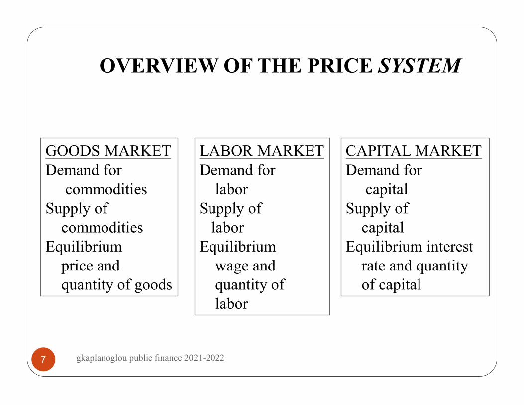
OVERVIEW OF THE PRICE SYSTEM
GOODS MARKETDemand for
commoditiesSupply of
commoditiesEquilibrium
price and quantity of goods
LABOR MARKETDemand for
laborSupply of
laborEquilibrium
wage and quantity of labor
CAPITAL MARKETDemand for
capitalSupply of
capitalEquilibrium interest
rate and quantity of capital
7 gkaplanoglou public finance 2021-2022

OVERVIEW OF THE PRICE SYSTEM
GOODS MARKETDemand for commoditiesSupply of commoditiesEquilibrium price and quantity of goods
LABOR MARKETDemand for laborSupply of laborEquilibrium wageand quantity of labor
CAPITAL MARKETDemand for capitalSupply of capitalEquilibrium interest rateand quantity of capital
GOVERNMENT
Excise TaxesPollution Taxes
Payroll TaxesMinimum Wage
Social SecurityCapital Gains Taxes
8 gkaplanoglou public finance 2021-2022
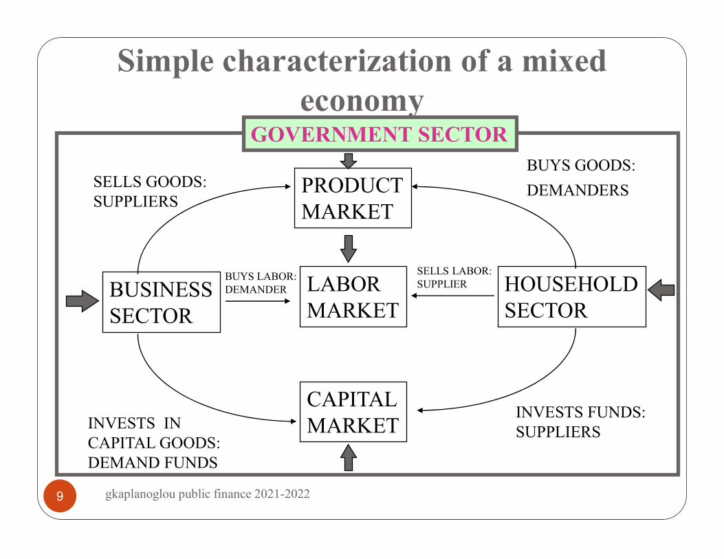
Simple characterization of a mixed economy
• *PRODUCTMARKET
HOUSEHOLDSECTOR
CAPITALMARKET
BUSINESSSECTOR
LABORMARKET
SELLS GOODS:SUPPLIERS
BUYS GOODS:
DEMANDERS
BUYS LABOR:DEMANDER
SELLS LABOR:SUPPLIER
INVESTS FUNDS:SUPPLIERSINVESTS IN
CAPITAL GOODS:DEMAND FUNDS
GOVERNMENT SECTOR
9 gkaplanoglou public finance 2021-2022

Simple characterization of a mixed economy
• *PRODUCTMARKET
HOUSEHOLDSECTOR
CAPITALMARKET
BUSINESSSECTOR
LABORMARKET
SELLS GOODS:SUPPLIERS
BUYS GOODS:
DEMANDERS
BUYS LABOR:DEMANDER
SELLS LABOR:SUPPLIER
INVESTS FUNDS:SUPPLIERSINVESTS IN
CAPITAL GOODS:DEMAND FUNDS
GOVERNMENT SECTORExternal Force
10 gkaplanoglou public finance 2021-2022
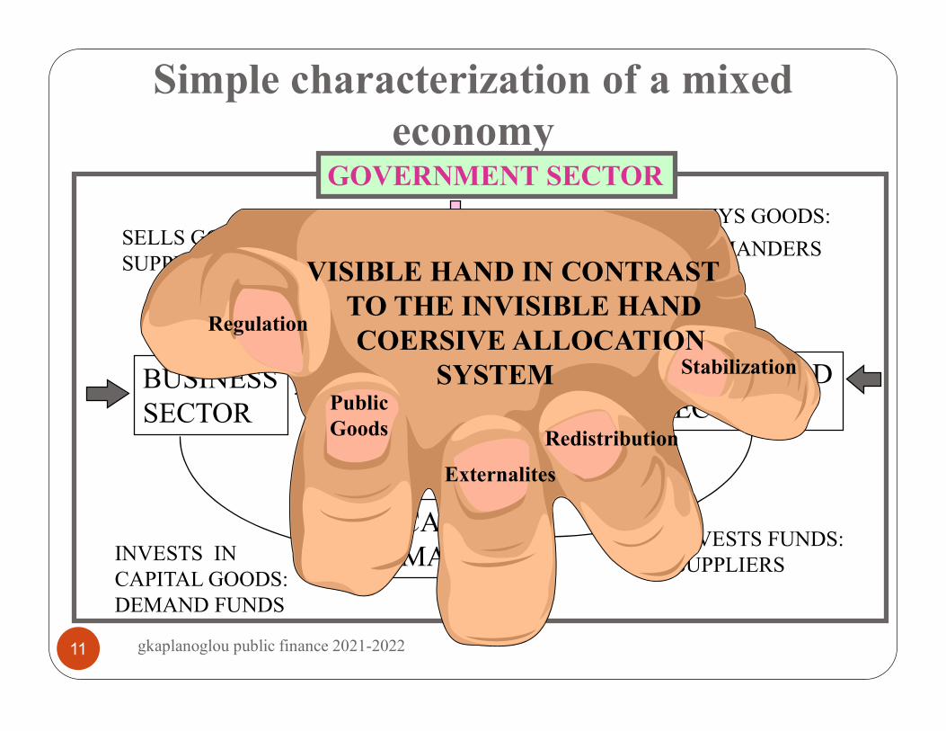
Simple characterization of a mixed economy
• *PRODUCTMARKET
HOUSEHOLDSECTOR
CAPITALMARKET
BUSINESSSECTOR
LABORMARKET
SELLS GOODS:SUPPLIERS
BUYS GOODS:
DEMANDERS
BUYS LABOR:DEMANDER
SELLS LABOR:SUPPLIER
INVESTS FUNDS:SUPPLIERSINVESTS IN
CAPITAL GOODS:DEMAND FUNDS
GOVERNMENT SECTOR
VISIBLE HAND IN CONTRASTTO THE INVISIBLE HANDCOERSIVE ALLOCATION
SYSTEM PublicGoods
Externalites
Redistribution
Regulation
Stabilization
11 gkaplanoglou public finance 2021-2022
Efficiency criterion
Positive Economics is the scientific view of economic events. It tries to find cause and effect, predictive relationships.
Normative Economics is based on value judgments. It tries to formulate recommendations as to what should be.
The efficiency criterion is satisfied when resources are used over a given period of time in such away as to make it impossible to increase the well-being of any one person without reducing the well-being of any other person. This situation is referred to as a Pareto Optimum state
.
12 gkaplanoglou public finance 2021-2022
Efficiency criterion
Definition: An allocation of resources is Pareto Efficient if it is not possible to reallocate resources to make everyone better off.
How do we measure better off?
We use Utility to measure welfare/happiness.
13 gkaplanoglou public finance 2021-2022
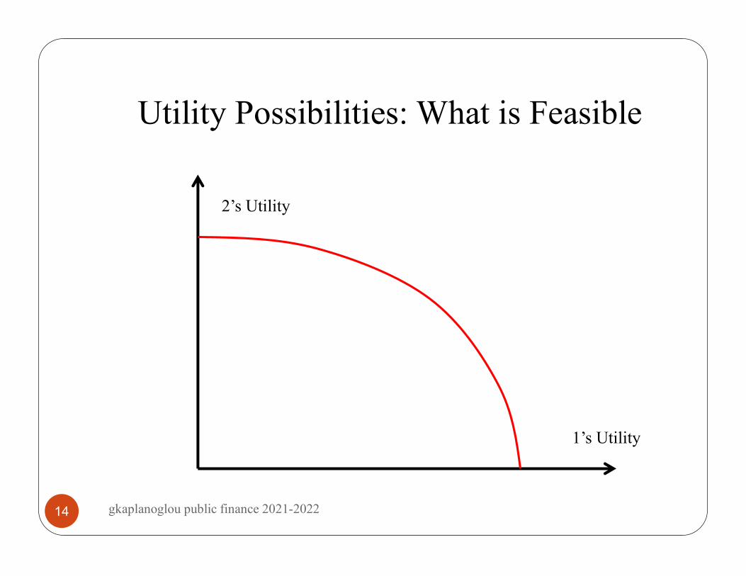
Utility Possibilities: What is Feasible
1’s Utility
2’s Utility
14 gkaplanoglou public finance 2021-2022
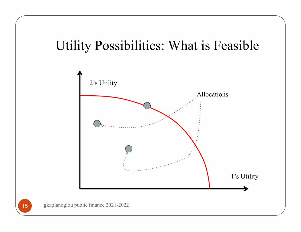
Utility Possibilities: What is Feasible
1’s Utility
2’s Utility
Allocations
15 gkaplanoglou public finance 2021-2022
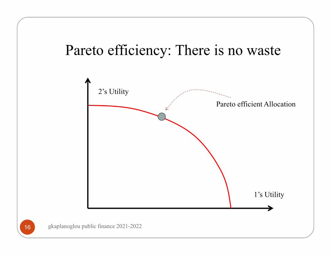
Pareto efficiency: There is no waste
1’s Utility
2’s Utility
Pareto efficient Allocation
16 gkaplanoglou public finance 2021-2022
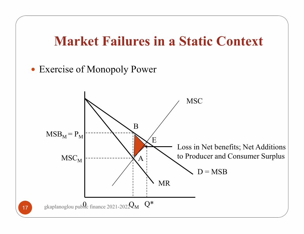
Market Failures in a Static Context
Exercise of Monopoly Power
D = MSB
MR
Q*QM
MSCM
MSBM = PM
MSC
A
E
B
Loss in Net benefits; Net Additionsto Producer and Consumer Surplus
017 gkaplanoglou public finance 2021-2022

Excise Tax and the Loss of Efficiency
MSC = MPC
MPC + T > MSC
Demand = MSB
Price
Units3 4
5
6
4
E’
E
B
18 gkaplanoglou public finance 2021-2022

Externalities
This case is the situation of positive and negative externalities. For example, exhaust fumes from automobiles, trucks and buses decreases air quality and impairs public health.
This cost is not reflected in marginal private costs. Thus inefficiency arises.
Education may create positive external benefits and in effect be under produced by the market.
19 gkaplanoglou public finance 2021-2022
Public goods
In many cases, useful goods and services cannot be provided efficiently through markets, because it is impossible or difficult to sell the good by the unit.
The benefits of such goods can be shared only.
Public goods are collective in consumption and can not be priced in the market.
20 gkaplanoglou public finance 2021-2022
Public goods
“Public” goods are distinguished from private goods in that private goods are consumed by individuals and whose benefits are not shared with others who do not make the purchase.
A distinguishing characteristic of public goods is that a given quantity of such goods can be enjoyed by additional consumers at no reduction in benefits to existing consumers.
21 gkaplanoglou public finance 2021-2022
Public goods
National defense is an example of a public good having this property. Increases in population occur daily; and the additional population can be defended without any reduction in benefits to the existing population.
Another characteristic of public goods is that their benefits cannot be easily withheld from persons who choose not to contribute to their finance.
22 gkaplanoglou public finance 2021-2022

Public goods: Free-Rider Issue in Public Goods
Even if you refuse to pay the costs of national defense, you still will be defended. This means that firms selling public goods like national defense will have great difficulty collecting revenue necessary to finance costs of production for such goods.
In many cases, government provision of goods is justified because of a conviction that the marginal social benefit of the good exceeds the marginal social cost at quantities that would result if the good were supplied through markets.
For example, government provision of health insurance, deposit insurance, and flood insurance are common because many persons believe that these are useful services that cannot be provided profitably in efficient amount by profit-maximizing firms.
23 gkaplanoglou public finance 2021-2022

Incomplete Information
Whenever private markets fail to provide a good or service even though the cost of providing it is less than what individuals are willing to pay
Examples: insurance and capital markets
Reasons: innovation, transaction costs, asymmetry of information and enforcement costs
The reason why markets do not exist may have implications for how governments might go about remedying the market failure
24 gkaplanoglou public finance 2021-2022

Incomplete Information
A number of government activities are motivated by imperfect information on the part of the consumers, and by the belief that the market, by itself, will supply too little information (e.g. regulations on information disclosure)
Information is, in many respects, a public good: the private market will often provide an inadequate supply of information, just as it supplies an inadequate amount of other public goods.
25 gkaplanoglou public finance 2021-2022
Macroeconomic failures
Unemployment
Inflation
26 gkaplanoglou public finance 2021-2022

Optimality conditions
• Marginal Condition for Exchange.
• To attain a Pareto Maximum, the marginal rate of substitution ( MRS ) between any pair of goods must be the same for all individuals who consume both goods.
27 gkaplanoglou public finance 2021-2022
Optimality conditions
Marginal Condition for Factor Substitution.
To attain Pareto Maximum, the marginal rate of technical substitution ( MRTS ) between any pair of inputs must be the same for all producers who use both inputs.
28 gkaplanoglou public finance 2021-2022

Optimality conditions
Marginal Condition for Product Substitution.
To attain a Pareto Maximum, the marginal rate of transformation ( MRT ) in production must equal the marginal rate of substitution in consumption for every pair of commodities and for every individual who consumes both.
29 gkaplanoglou public finance 2021-2022
Optimality conditions
Corollary Proposition.
If the political organization of a society is such to accord paramount importance to its individual members -- mechanistic approach to government --social welfare will be maximized if every consumer, every firm, and every input market is perfectly competition.
30 gkaplanoglou public finance 2021-2022

CONSTRAINED UTILITY MAXIMIZATION
Constrained utility maximization means that all decisions are made in order to maximize the well-being of the individual, subject to his available resources.
Utility maximization involves preferences and a budget constraint.
One of the key assumptions about preferences is non-satiation–that “more is preferred to less.”
31 gkaplanoglou public finance 2021-2022
Constrained Utility Maximization:Preferences and indifference curves
Figure 1 illustrates some preferences over movies (on the x-axis) and CDs (on the y-axis).
Because of non-satiation, bundles A and B are both inferior to bundle C.
32 gkaplanoglou public finance 2021-2022
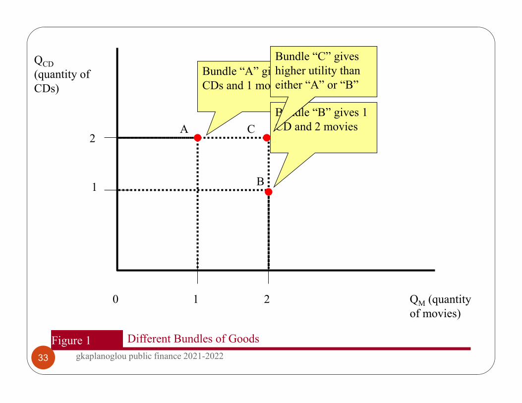
Figure 1 Different Bundles of Goods
QM (quantity of movies)
QCD
(quantity of CDs)
0 1 2
1
2
Bundle “A” gives 2 CDs and 1 movie
A
B
Bundle “B” gives 1 CD and 2 moviesC
Bundle “C” gives 2 CDs and 2 moviesBundle “C” gives higher utility than either “A” or “B”
33 gkaplanoglou public finance 2021-2022
Constrained Utility Maximization: Preferences and indifference curves
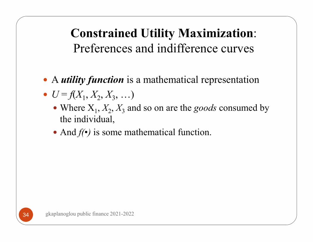
A utility function is a mathematical representation
U = f(X1, X2, X3, …) Where X1, X2, X3 and so on are the goods consumed by
the individual, And f(•) is some mathematical function.
34 gkaplanoglou public finance 2021-2022
Constrained Utility Maximization:Preferences and indifference curves
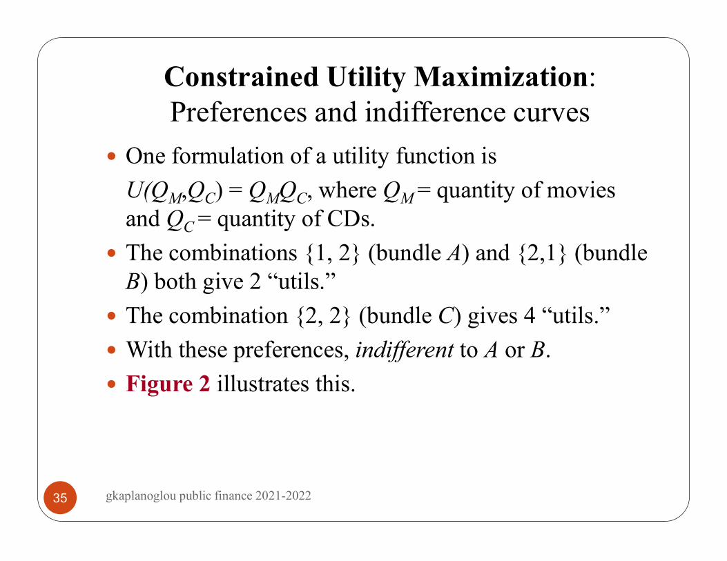
One formulation of a utility function is
U(QM,QC) = QMQC, where QM = quantity of movies and QC = quantity of CDs.
The combinations {1, 2} (bundle A) and {2,1} (bundle B) both give 2 “utils.”
The combination {2, 2} (bundle C) gives 4 “utils.”
With these preferences, indifferent to A or B.
Figure 2 illustrates this.
35 gkaplanoglou public finance 2021-2022

Figure 2 Utility From Different Bundles
QM (quantity of movies)
QCD
(quantity of CDs)
0 1 2
1
2A
B
C
IC1
IC2
“A” and “B” both give 2 “utils” and lie on the same indifference curve
Bundle “C” gives higher utility than either “A” or “B”
Bundle “C” gives 4 “utils” and is on a higher indifference curve
Higher utility as move toward northeast in the quadrant.
36 gkaplanoglou public finance 2021-2022

Constrained Utility Maximization:Utility mapping of preferences
How are indifference curves derived?
Set utility equal to a constant level and figure out the bundles of goods that get that utility level.
For U = QMQC, how would we find the bundles for the indifference curve associated with 25 utils? Set 25 = QMQC, Yields QC = 25/QM, Or bundles like {1,25}, {1.25,20}, {5,5}, etc.
37 gkaplanoglou public finance 2021-2022

Constrained Utility Maximization: Marginal utility
Marginal utility is the additional increment to utility from consuming an additional unit of a good.
Diminishing marginal utility means each additional unit makes the individual less happy than the previous unit.
38 gkaplanoglou public finance 2021-2022

Constrained Utility Maximization: Marginal utility
With the utility function given before, U = QMQC, the marginal utility is:
Take the partial derivative of the utility function with respect to QM to get the marginal utility of movies.
MUU
QQQ
MCM
39gkaplanoglou public finance 2021-2022
Constrained Utility Maximization:Marginal utility
Evaluating the utility function U = (QMQC)1/2, at QC = 2 allows us to plot a relationship between marginal utility and movies consumed.
Figure 3 illustrates this.
40 gkaplanoglou public finance 2021-2022
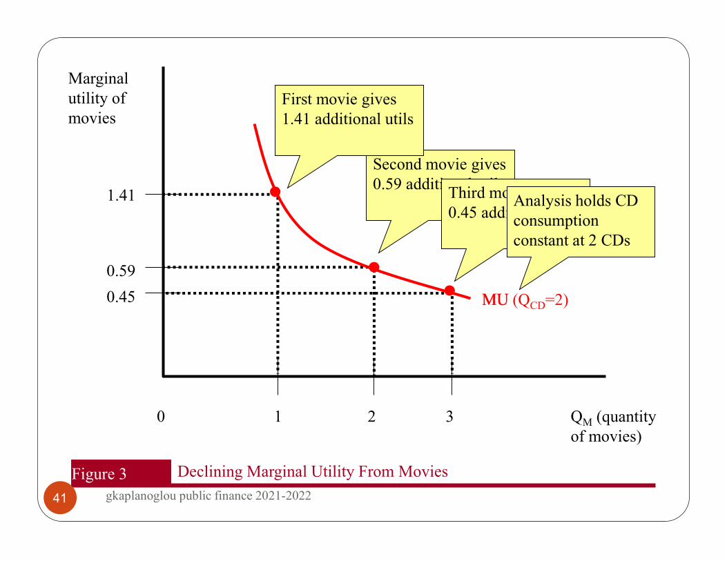
MU (QCD=2)
Figure 3 Declining Marginal Utility From Movies
QM (quantity of movies)
Marginal utility of movies
0 1 2
0.59
1.41
MU
3
0.45
Second movie gives 0.59 additional utils
First movie gives 1.41 additional utils
Third movie gives 0.45 additional utils
Analysis holds CD consumption constant at 2 CDs
41 gkaplanoglou public finance 2021-2022

Constrained Utility Maximization:Marginal utility
Why does diminishing marginal utility make sense? Most consumers order consumption of the goods with the
highest utility first.
42 gkaplanoglou public finance 2021-2022
Constrained Utility Maximization:Marginal rate of substitution
Marginal rate of substitution—slope of the indifference curve is called the MRS, and is the rate at which consumer is willing to trade off the two goods.
Returning to the (CDs, movies) example.
Figure 4 illustrates this.
43 gkaplanoglou public finance 2021-2022
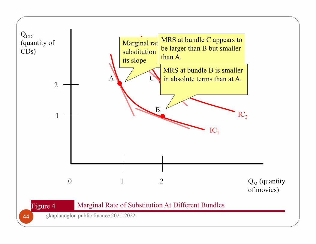
Figure 4 Marginal Rate of Substitution At Different Bundles
QM (quantity of movies)
QCD
(quantity of CDs)
0 1 2
1
2A
B
C
IC1
IC2
Marginal rate of substitution at bundle A is its slope
MRS at bundle C appears to be larger than B but smaller than A.
MRS at bundle B is smaller in absolute terms than at A.
44 gkaplanoglou public finance 2021-2022
Constrained Utility Maximization:Marginal rate of substitution
MRS is diminishing (in absolute terms) as we move along an indifference curve.
This means that Andrea is willing to give up fewer CD’s to get more movies when she has more movies (bundle B) than when she has less movies (bundle A).
Figure 5 illustrates this.
45 gkaplanoglou public finance 2021-2022

Figure 5 Marginal Rate of Substitution is Diminishing
QM (quantity of movies)
QCD
(quantity of CDs)
0 1 2
1
2A
B
IC1
3
D
Willing to give up a lot of CDs for another movie …
Not willing to give up very many CDs for another movie Even less willing to give up
additional CDs
46 gkaplanoglou public finance 2021-2022

Constrained Utility Maximization:Marginal rate of substitution
Direct relationship between MRS and marginal utility.
MRS shows how the relative marginal utilities evolve over the indifference curve.
Straightforward to derive this relationship graphically, as well.
Consider the movement from bundle A to bundle B. Figure 6 illustrates this.
MRSMU
MUM
C
47gkaplanoglou public finance 2021-2022

Figure 6 Relationship Between Marginal Utility and MRS
QM (quantity of movies)
QCD
(quantity of CDs)
0 1 2
1
2A
B
IC1
3
Movement down is change in CDs, ΔQC.
Must have MUCΔQC=MUMΔQM
because we are on the same indifference curve.Gain in utility from more movies is MUMΔQM.
Simply rearrange the equation to get the relationship between MRSand marginal utilities.
Moving from A to B does not change utility
Movement across is change in movies, ΔQM.
Loss in utility from less CDs is MUCΔQC.
48 gkaplanoglou public finance 2021-2022

Constrained Utility Maximization:Budget constraints
The budget constraint is a mathematical representation of the combination of goods the consumer can afford to buy with a given income.
Assume there is no saving or borrowing.
In the example, denote: Y = Income level PM = Price of one movie PC = Price of one CD
49 gkaplanoglou public finance 2021-2022
Constrained Utility Maximization:Budget constraints
The expenditure on movies is:
While the expenditure on CDs is:
P QM M
P QC C
50gkaplanoglou public finance 2021-2022

Constrained Utility Maximization:Budget constraints
Thus, the total amount spent is:
This must equal income, because of no saving or borrowing.
P Q P QM M C C
Y P Q P QM M C C
51gkaplanoglou public finance 2021-2022

Constrained Utility Maximization:Budget constraints
This budget constraint is illustrated in the next figure.
Figure 7 illustrates this.
52 gkaplanoglou public finance 2021-2022
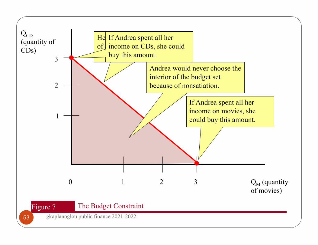
Figure 7 The Budget Constraint
QM (quantity of movies)
QCD
(quantity of CDs)
0 1 2
1
2
3
3
If Andrea spent all her income on movies, she could buy this amount.
Andrea would never choose the interior of the budget set because of nonsatiation.
Her budget constraint consists of all combinations on the red line.
If Andrea spent all her income on CDs, she could buy this amount.
53 gkaplanoglou public finance 2021-2022
Constrained Utility Maximization:Budget constraints
The slope of the budget constraint is:
It is thought that government actions can change a consumer’s budget constraint, but that a consumer’s preferences are fixed.
P
PM
C
54gkaplanoglou public finance 2021-2022

Constrained Utility Maximization:Putting it together: Constrained choice
What is the highest indifference curve that an individual can reach, given a budget constraint?
Preferences tells us what a consumer wants, and the budget constraint tells us what a consumer can actually purchase.
This leads to utility maximization, shown graphically, in Figure 8.
55 gkaplanoglou public finance 2021-2022
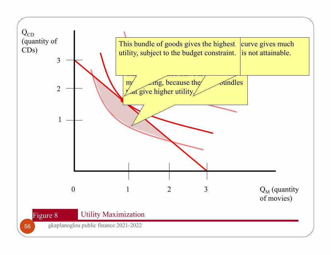
Figure 8 Utility Maximization
QM (quantity of movies)
QCD
(quantity of CDs)
0 1 2
1
2
3
3
This indifference curve is not utility-maximizing, because there are bundles that give higher utility.
This indifference curve gives much higher utility, but is not attainable.
This bundle of goods gives the highest utility, subject to the budget constraint.
56 gkaplanoglou public finance 2021-2022
Constrained Utility Maximization:Putting it together: Constrained choice
In this figure, the utility maximizing choice occurs where the indifference curve is tangent to the budget constraint.
This implies that the slope of the indifference curve equals the slope of the budget constraint.
57 gkaplanoglou public finance 2021-2022
Constrained Utility Maximization:Putting it together: Constrained choice
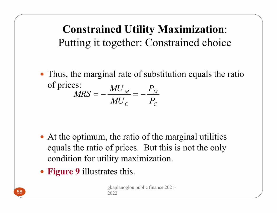
Thus, the marginal rate of substitution equals the ratio of prices:
At the optimum, the ratio of the marginal utilities equals the ratio of prices. But this is not the only condition for utility maximization.
Figure 9 illustrates this.
MRSMU
MU
P
PM
C
M
C
58gkaplanoglou public finance 2021-2022

Figure 9 MRS Equal to Price Ratio is Insufficient
QM (quantity of movies)
QCD
(quantity of CDs)
0 1 2
1
2
3
3
The MRS equals the price ratio at this bundle, but is unaffordable.
The MRS equals the price ratio at this bundle, but it wastes resources.
59 gkaplanoglou public finance 2021-2022
Constrained Utility Maximization:Putting it together: Constrained choice
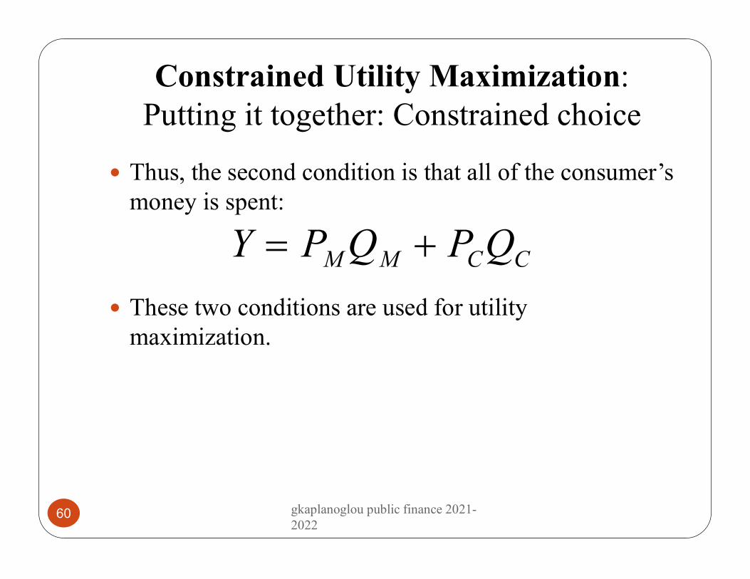
Thus, the second condition is that all of the consumer’s money is spent:
These two conditions are used for utility maximization.
Y P Q P QM M C C
60 gkaplanoglou public finance 2021-2022
The Effects of Price Changes:Substitution and income effects
Consider a typical price change in our framework:
Increase the price of movies, PM.
This rotates the budget constraint inward along the x-axis.
Figure 10 illustrates this.
61 gkaplanoglou public finance 2021-2022

Figure 10 Increase in the Price of Movies
QM (quantity of movies)
QCD
(quantity of CDs)
0 1 2
1
2
3
3
Increase in PM rotates the budget constraint inward on x-axis.Andrea is worse off, and consumes less movies.
62 gkaplanoglou public finance 2021-2022

The Effects of Price Changes:Substitution and income effects
A change in price consists of two effects:
Substitution effect–change in consumption due to change in relative prices, holding utility constant.
Income effect–change in consumption due to feeling “poorer” after price increase.
Figure 11 illustrates this.
63 gkaplanoglou public finance 2021-2022

Figure 11 Illustration of Income and Substitution Effects
QM (quantity of movies)
QCD
(quantity of CDs)
0 1 2
1
2
3
3
Movement along the indifference curve is the substitution effect
Movement from one indifference curve to the other is the income effect.
Decline in QM due to substitution effectDecline in QM due to income effect
64 gkaplanoglou public finance 2021-2022
EQUILIBRIUM AND SOCIAL WELFARE
Welfare economics is the study of the determinants of well-being, or welfare, in society. It depends on:
Determinants of social efficiency, or size of the economic “pie.”
Redistribution.
65 gkaplanoglou public finance 2021-2022
EQUILIBRIUM AND SOCIAL WELFAREDemand curves
Demand curve is the relationship between the price of a good and the quantity demanded.
Derive demand curve from utility maximization problem, as shown in Figure 18.
66 gkaplanoglou public finance 2021-2022

Figure 18 Increase in the Price of Movies
QM (quantity of movies)
QCD (quantity of CDs)
QM,1QM,2QM,3
Raising PM even more gives another (PM,QM) combination with even less movies demanded.
Raising PM gives another (PM,QM) combination with fewer movies demanded.
Initial utility-maximizing point gives one (PM,QM) combination.
67 gkaplanoglou public finance 2021-2022
EQUILIBRIUM AND SOCIAL WELFARE
Demand curves This gives various (PM,QM) combinations that can be
mapped into price/quantity space.
This gives us the demand curve for movies.
Figure 19 illustrates this.
68 gkaplanoglou public finance 2021-2022
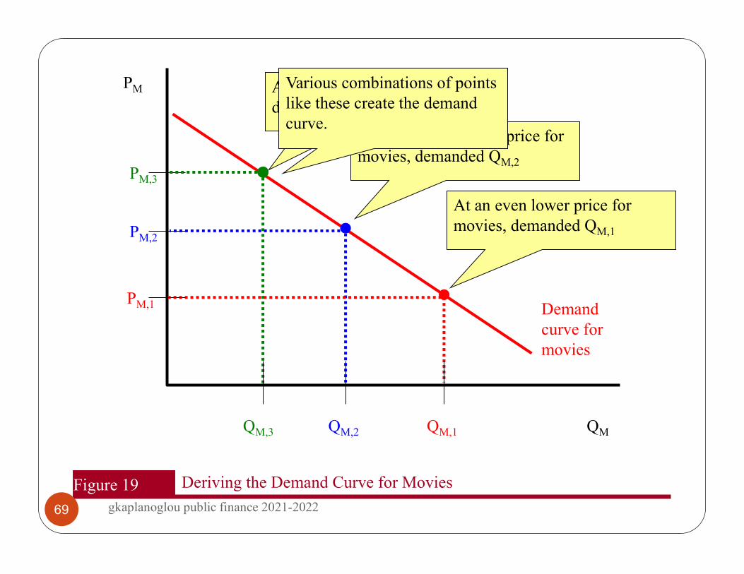
Figure 19 Deriving the Demand Curve for Movies
QM
PM
QM,3
Demand curve for movies
At a high price for movies, demanded QM,3
PM,3
At a somewhat lower price for movies, demanded QM,2
QM,2
PM,2
At an even lower price for movies, demanded QM,1
QM,1
PM,1
Various combinations of points like these create the demand curve.
69 gkaplanoglou public finance 2021-2022

EQUILIBRIUM AND SOCIAL WELFARE
Elasticity of demand
A key feature of demand analysis is the elasticity of demand. It is defined as:
That is, the percent change in quantity demanded divided by the percent change in price.
D
D
D
PP
70gkaplanoglou public finance 2021-2022
EQUILIBRIUM AND SOCIAL WELFARE
Elasticity of demand For example, an increase in the price of movies from
€ 8 to €12 is a 50% rise in price. If the number of movies purchased fell from 6 to 4,
there is an associated 33% reduction in quantity demanded. The demand elasticity is therefore -0.67.
Demand elasticities features: Typically negative number. Not constant along the demand curve (for a linear
demand curve).
71 gkaplanoglou public finance 2021-2022

EQUILIBRIUM AND SOCIAL WELFARE
Elasticity of demand For a vertical demand curve
Elasticity of demand is zero—quantity does not change as price goes up or down.
Perfectly inelastic
For a horizontal demand curve Elasticity of demand is negative infinity—quantity
changes infinitely for even a small change in price. Perfectly elastic
Figure 20 illustrates this.
72 gkaplanoglou public finance 2021-2022
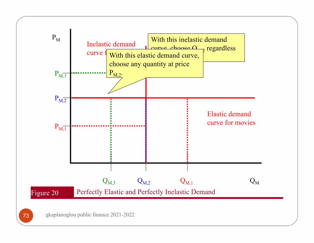
Figure 20 Perfectly Elastic and Perfectly Inelastic Demand
QM
PM
QM,3
Inelastic demand curve for movies
With this inelastic demand curve, choose QM,2 regardless of the price.
PM,3
QM,2
PM,2
QM,1
PM,1
With this elastic demand curve, choose any quantity at price PM,2.
Elastic demand curve for movies
73 gkaplanoglou public finance 2021-2022

EQUILIBRIUM AND SOCIAL WELFARE
Elasticity of demand
More generally, an elasticity divides the percent change in a dependent variable by the percent change in an independent variable:
For example, Y is often the quantity demanded or supplied, while X might be own-price, cross-price, or income.
YY
XX
74gkaplanoglou public finance 2021-2022

EQUILIBRIUM AND SOCIAL WELFARE
Supply curves Supply curve is the relationship between the price of a
good and the quantity supplied. Derive supply curve from profit maximization problem.
The firm’s production function measures the impact of a firm’s input use on output levels.
75 gkaplanoglou public finance 2021-2022
EQUILIBRIUM AND SOCIAL WELFARE
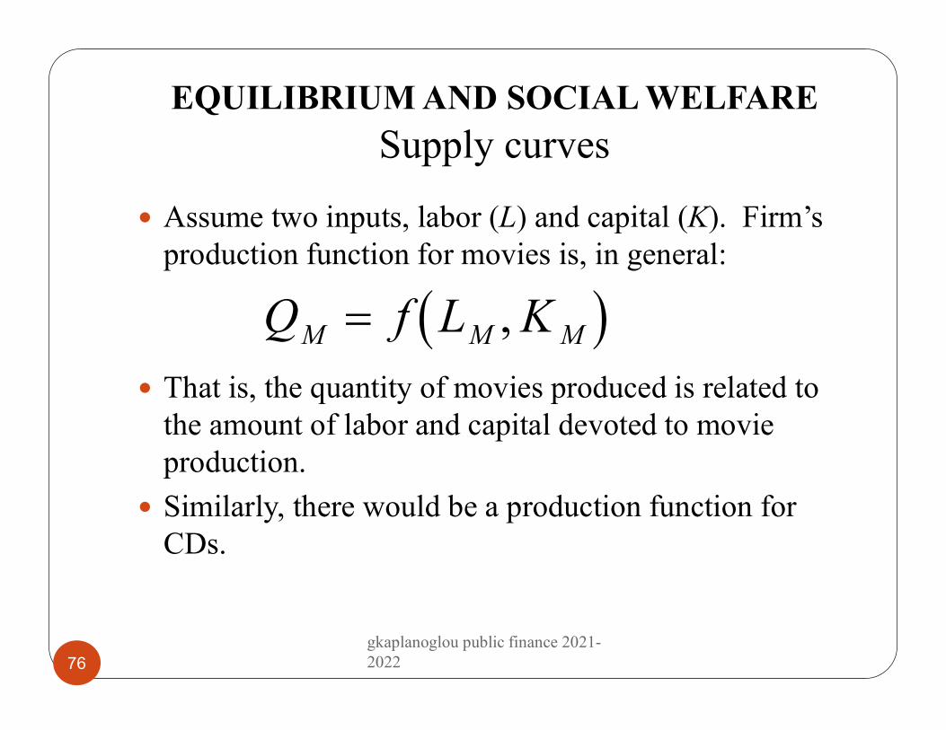
Supply curves
Assume two inputs, labor (L) and capital (K). Firm’s production function for movies is, in general:
That is, the quantity of movies produced is related to the amount of labor and capital devoted to movie production.
Similarly, there would be a production function for CDs.
Q f L KM M M ,
76gkaplanoglou public finance 2021-2022
EQUILIBRIUM AND SOCIAL WELFARE
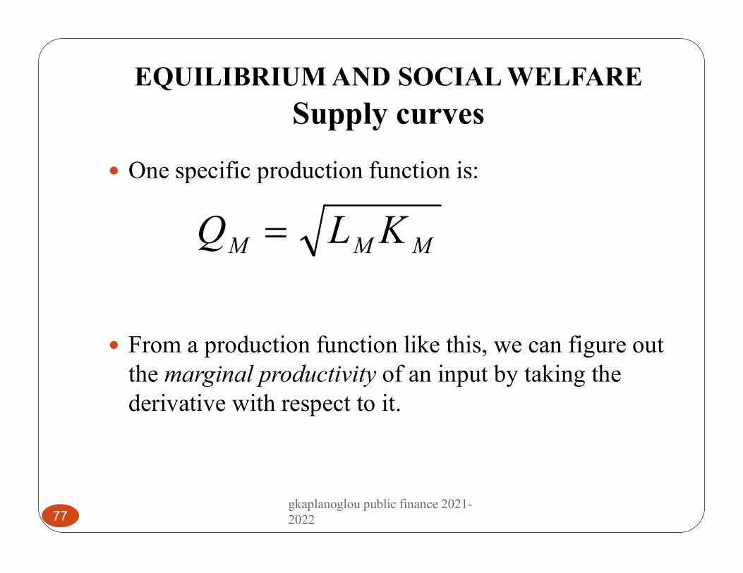
Supply curves
One specific production function is:
From a production function like this, we can figure out the marginal productivity of an input by taking the derivative with respect to it.
Q L KM M M
77gkaplanoglou public finance 2021-2022
Equilibrium and Social Welfare: Supply curves
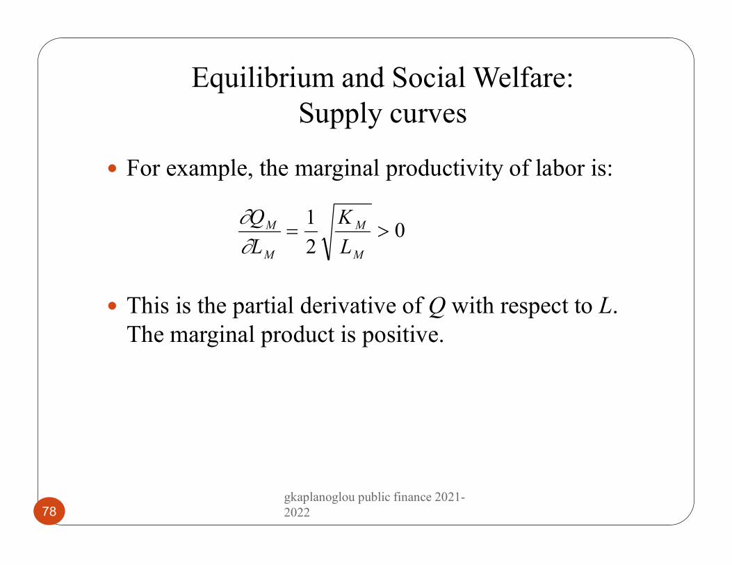
For example, the marginal productivity of labor is:
This is the partial derivative of Q with respect to L. The marginal product is positive.
Q
L
K
LM
M
M
M
1
20
78gkaplanoglou public finance 2021-2022
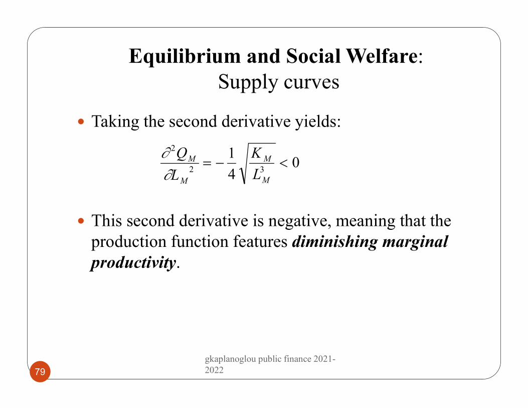
Equilibrium and Social Welfare:Supply curves
Taking the second derivative yields:
This second derivative is negative, meaning that the production function features diminishing marginal productivity.
2
2 3
1
40
Q
L
K
LM
M
M
M
79
gkaplanoglou public finance 2021-2022

EQUILIBRIUM AND SOCIAL WELFARE
Supply curves
Diminishing marginal productivity means that holding all other inputs constant, increasing the level of one input (such as labor) yields less and less additional output.
80 gkaplanoglou public finance 2021-2022

EQUILIBRIUM AND SOCIAL WELFARE
Supply curves
The total costs of production are given by:
In this case, r and w are the input prices of capital and labor, respectively.
TC rK wL
81gkaplanoglou public finance 2021-2022
EQUILIBRIUM AND SOCIAL WELFARE
Supply curves
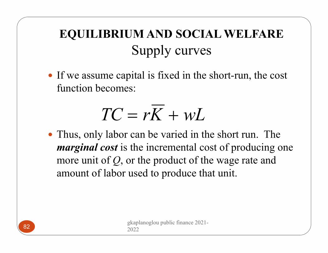
If we assume capital is fixed in the short-run, the cost function becomes:
Thus, only labor can be varied in the short run. The marginal cost is the incremental cost of producing one more unit of Q, or the product of the wage rate and amount of labor used to produce that unit.
TC rK wL
82gkaplanoglou public finance 2021-2022
EQUILIBRIUM AND SOCIAL WELFARE
Supply curves
Diminishing marginal productivity implies rising marginal costs.
Since each additional unit, Q, means calling forth less and less productive labor at the same wage rate, costs of production rise.
83 gkaplanoglou public finance 2021-2022
EQUILIBRIUM AND SOCIAL WELFARE
Supply curves
Profit maximization means maximizing the difference between total revenue and total costs.
This occurs at the quantity where marginal revenueequals marginal costs.
84 gkaplanoglou public finance 2021-2022

EQUILIBRIUM AND SOCIAL WELFARE
Equilibrium
In a perfectly competitive market, the marginal revenue is the market price. Thus, the firm produces until: P = MC.
Thus, the MC curve is the supply curve.
85 gkaplanoglou public finance 2021-2022

EQUILIBRIUM AND SOCIAL WELFARE
Equilibrium
In equilibrium, we horizontally sum individual demand curves to get aggregate demand.
We also horizontally sum individual supply curves to get aggregate supply.
Competitive equilibrium represents the point at which both consumers and suppliers are satisfied with the price/quantity combination.
Figure 21 illustrates this.
86 gkaplanoglou public finance 2021-2022

Figure 21 Equilibrium with Supply and Demand
QM
PM
QM,3
Demand curve for movies
PM,3
QM,2
PM,2
QM,1
PM,1
Supply curve of movies
Intersection of supply and demand is equilibrium.
87 gkaplanoglou public finance 2021-2022

EQUILIBRIUM AND SOCIAL WELFARE
Social efficiency
Measuring social efficiency is computing the potential size of the economic pie. It represents the net gain from trade to consumers and producers.
88 gkaplanoglou public finance 2021-2022
EQUILIBRIUM AND SOCIAL WELFARE
Social efficiency
Consumer surplus is the benefit that consumers derive from a good, beyond what they paid for it.
Each point on the demand curve represents a “willingness-to-pay” for that quantity.
Figure 22 illustrates this.
89 gkaplanoglou public finance 2021-2022

Figure 22 Deriving Consumer Surplus
QM
PM
0
Demand curve for movies
Q*
P*
Supply curve of movies
The willingness-to-pay for the first unit is very high.
1
Yet the actual price paid is much lower.
The willingness to pay for the second unit is a bit lower.
2
The consumer surplus at Q* is the area between the demand curve and market price.
The total consumer surplus is this triangle.
The consumer’s “surplus” from the next unit is this trapezoid.
There is still surplus, because the price is lower.
The consumer’s “surplus” from the first unit is this trapezoid.
90 gkaplanoglou public finance 2021-2022
EQUILIBRIUM AND SOCIAL WELFARE
Social efficiency
Consumer surplus is determined by market price and the elasticity of demand: With inelastic demand, demand curve is more vertical, so
surplus is higher. With elastic demand, surplus is lower.
Figure 23 illustrates this.
91 gkaplanoglou public finance 2021-2022

Figure 23 Consumer Surplus and Inelastic Demand
QM
PM
0
Demand curve for movies
Q*
P*
Supply curve of movies
Consumer surplus is larger when demand curve is more inelastic.
1 2
92 gkaplanoglou public finance 2021-2022

EQUILIBRIUM AND SOCIAL WELFARE
Social efficiency
Producer surplus is the benefit derived by producers from the sale of a unit above and beyond their cost of producing it.
Each point on the supply curve represents the marginal cost of producing it.
Figure 24 illustrates this.
93 gkaplanoglou public finance 2021-2022
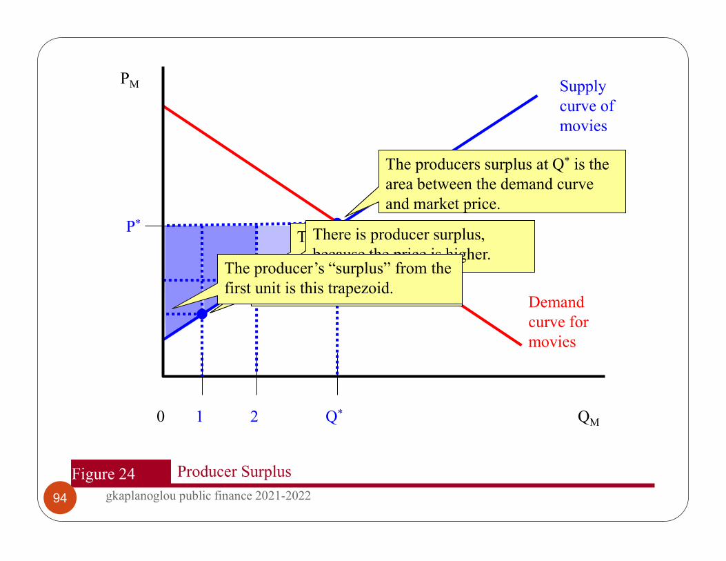
Figure 24 Producer Surplus
QM
PM
0
Demand curve for movies
Q*
P*
Supply curve of movies
1 2
The total producer’s surplus is this triangle.
The producer’s “surplus” from the next unit is this trapezoid.
The marginal cost for the second unit is a bit higher.There is producer surplus, because the price is higher.
The producers surplus at Q* is the area between the demand curve and market price.
Yet the actual price received is much higher.The marginal cost for the first unit is very low.
The producer’s “surplus” from the first unit is this trapezoid.
94 gkaplanoglou public finance 2021-2022
EQUILIBRIUM AND SOCIAL WELFARE
Social efficiency
Similar to consumer surplus, producer surplus is determined by market price and the elasticity of supply: With inelastic supply, supply curve is more vertical, so
producer surplus is higher. With elastic supply, producer surplus is lower.
95 gkaplanoglou public finance 2021-2022
EQUILIBRIUM AND SOCIAL WELFARE
Social efficiency
The total social surplus, also known as “social efficiency,” is the sum of the consumer’s and producer’s surplus.
Figure 25 illustrates this.
96 gkaplanoglou public finance 2021-2022
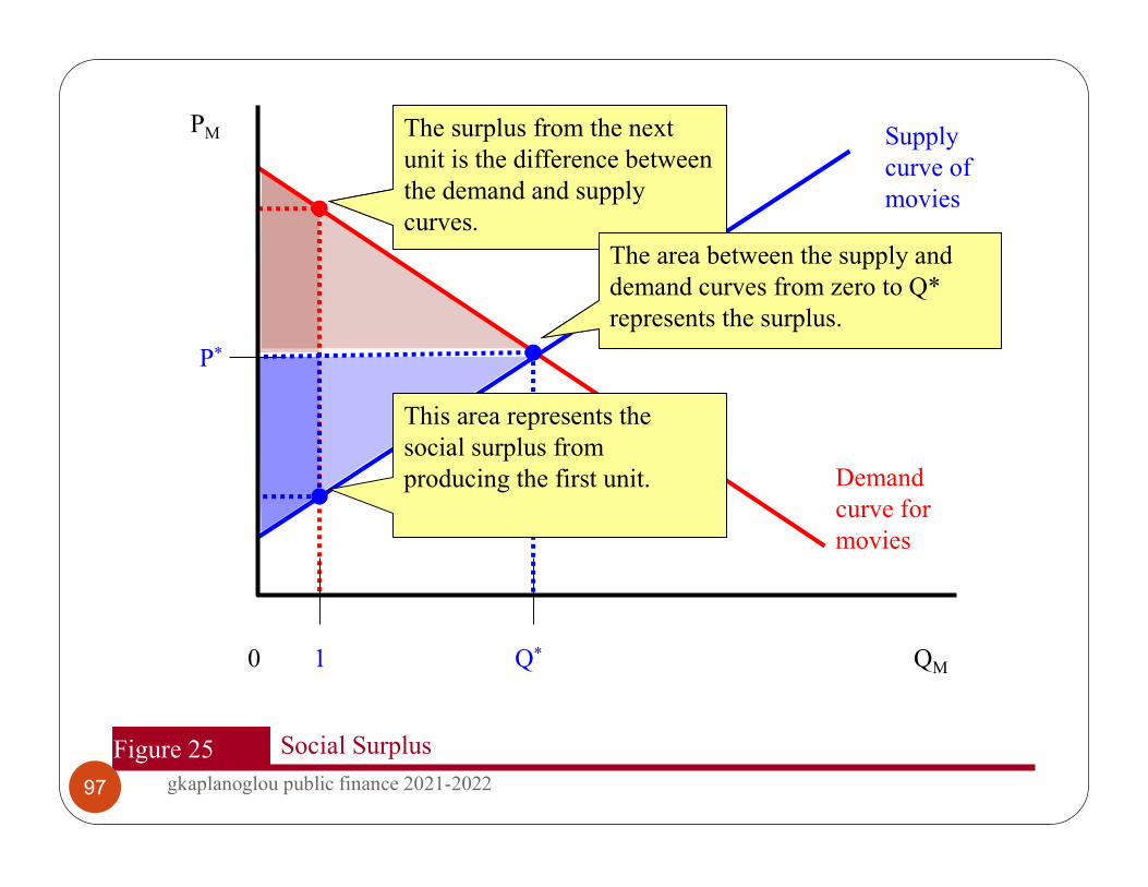
Figure 25 Social Surplus
QM
PM
0
Demand curve for movies
Q*
P*
Supply curve of movies
Providing the first unit gives a great deal of surplus to “society.”
1
Social efficiency is maximized at Q*, and is the sum of the consumer and producer surplus.
The surplus from the next unit is the difference between the demand and supply curves.
This area represents the social surplus from producing the first unit.
The area between the supply and demand curves from zero to Q* represents the surplus.
97 gkaplanoglou public finance 2021-2022

EQUILIBRIUM AND SOCIAL WELFARECompetitive equilibrium maximizes social efficiency
The First Fundamental Theorem of Welfare Economics states that the competitive equilibrium, where supply equals demand, maximizes social efficiency.
Any quantity other than Q* reduces social efficiency, or the size of the “economic pie.”
Consider restricting the price of the good to P´<P*.
Figure 26 illustrates this.
98 gkaplanoglou public finance 2021-2022

Figure 26 Deadweight Loss from a Price Floor
QM
PM
Demand curve for movies
Q*
P*
Supply curve of movies
Q´
P´
The social surplus from Q’ is this area, consisting of a larger consumer and smaller producer surplus.
With such a price restriction, the quantity falls to Q´, and there is excess demand.
This triangle represents lost surplus to society, known as “deadweight loss.”
99 gkaplanoglou public finance 2021-2022
EQUILIBRIUM AND SOCIAL WELFARECompetitive equilibrium maximizes social efficiency
A policy like price controls creates deadweight loss, the reduction in social efficiency by restricting quantity below the competitive equilibrium.
100 gkaplanoglou public finance 2021-2022

EQUILIBRIUM AND SOCIAL WELFARE
The role of equity
Societies usually care not only about how much surplus there is, but also about how it is distributed among the population.
Social welfare is determined by both criteria. The Second Fundamental Theorem of Welfare
Economics states that society can attain any efficient outcome by a suitable redistribution of resources and free trade.
In reality, society often faces an equity-efficiency tradeoff.
101 gkaplanoglou public finance 2021-2022

EQUILIBRIUM AND SOCIAL WELFAREThe role of equity
Society’s tradeoffs of equity and efficiency are models with a Social Welfare Function.
This maps individual utilities into an overall social utility function.
102 gkaplanoglou public finance 2021-2022
EQUILIBRIUM AND SOCIAL WELFAREThe role of equity
The utilitarian social welfare function is:
The utilities of all individuals are given equal weight.
Implies that government should transfer from person 1 to person 2 as long as person 2’s gain is bigger than person 1’s loss in utility.
SWF Uii
103gkaplanoglou public finance 2021-2022

EQUILIBRIUM AND SOCIAL WELFAREThe role of equity
Utilitarian SWF is defined in terms of utility, not euros.
Society not indifferent between giving €1 of income to rich and poor; rather indifferent between one util to rich and one util to poor.
104 gkaplanoglou public finance 2021-2022
EQUILIBRIUM AND SOCIAL WELFAREThe role of equity
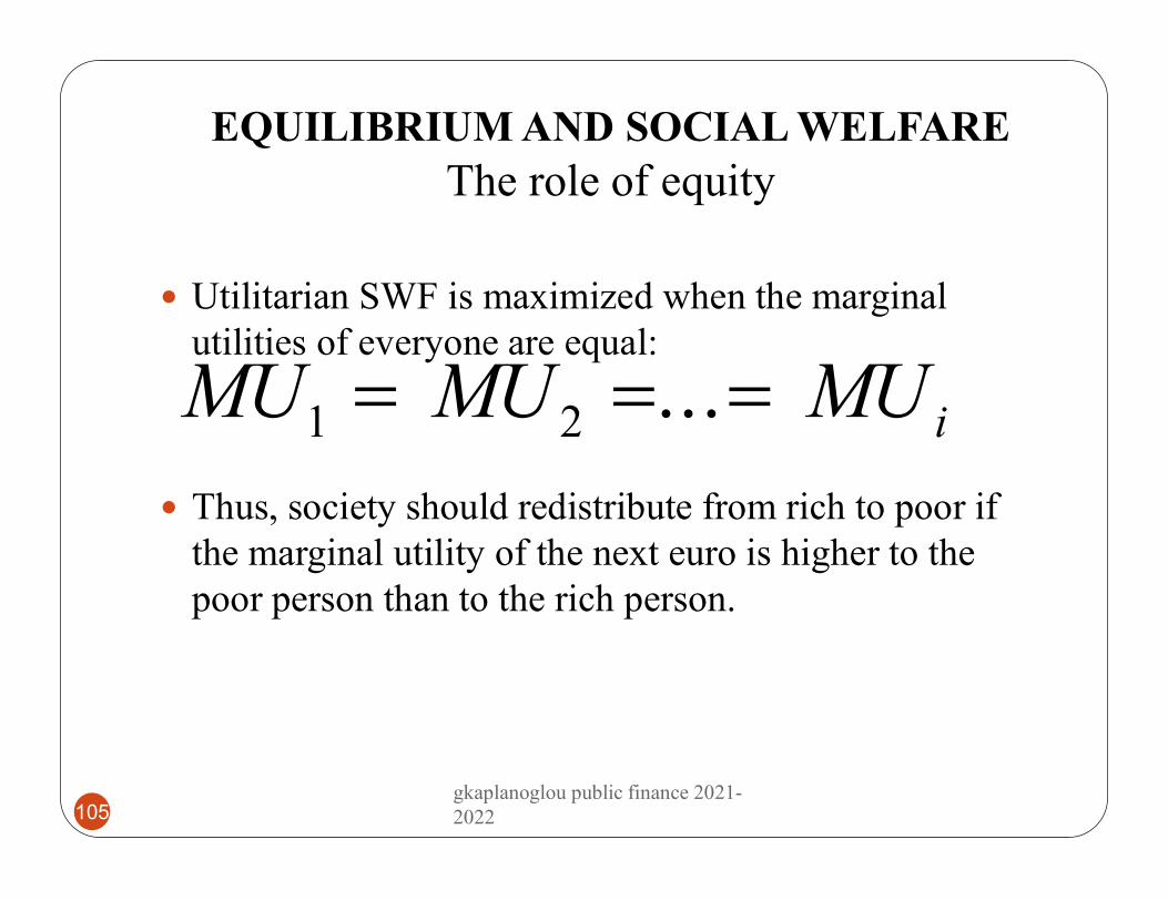
Utilitarian SWF is maximized when the marginal utilities of everyone are equal:
Thus, society should redistribute from rich to poor if the marginal utility of the next euro is higher to the poor person than to the rich person.
MU MU MUi1 2 ...
105gkaplanoglou public finance 2021-2022

EQUILIBRIUM AND SOCIAL WELFAREThe role of equity
The Rawlsian social welfare function is:
Societal welfare is maximized by maximizing the well-being of the worst-off person in society.
Generally suggests more redistribution than the utilitarian SWF.
SWF U U U N min , , ...,1 2
106gkaplanoglou public finance 2021-2022

Equity: equal shares
1’s Utility
2’s Utility U1 = U2
107 gkaplanoglou public finance 2021-2022
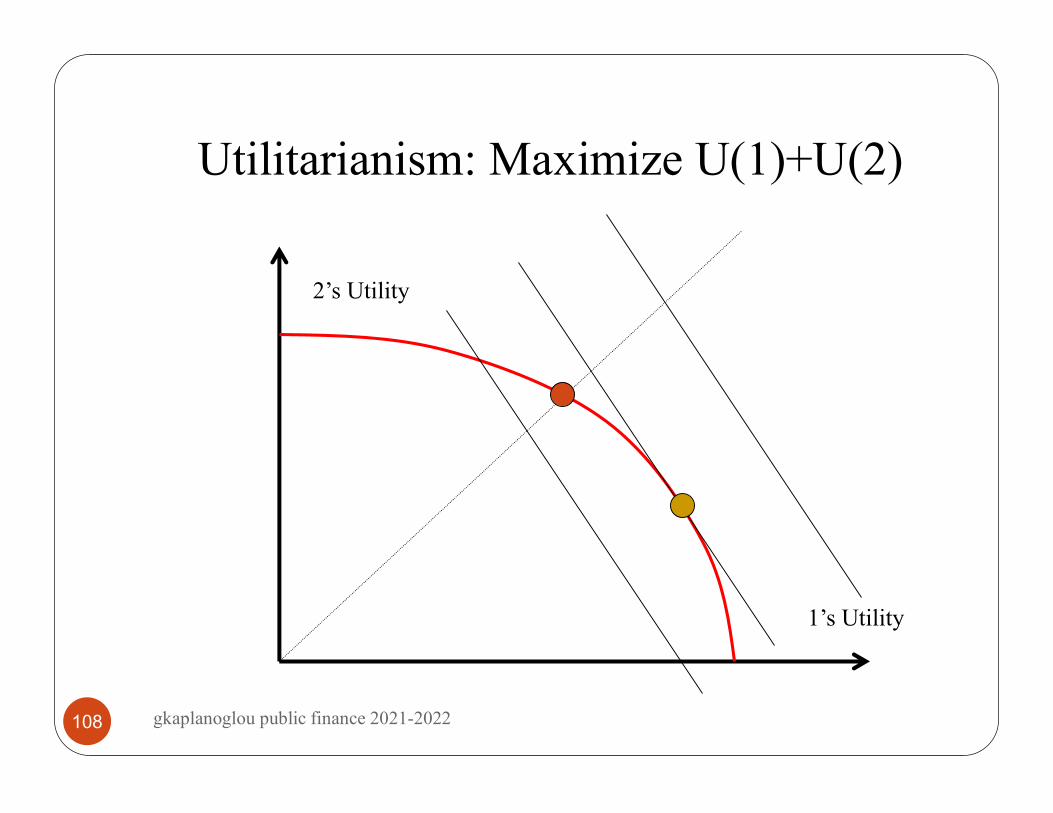
Utilitarianism: Maximize U(1)+U(2)
1’s Utility
2’s Utility
108 gkaplanoglou public finance 2021-2022

Rawls: Maximize min{U(1),U(2)}
1’s Utility
2’s Utility
109 gkaplanoglou public finance 2021-2022

Recap of Theoretical Tools Utility maximization
Labor supply example
Efficiency
Social welfare functions
110 gkaplanoglou public finance 2021-2022
Related Documents