Lecture 2: Filtering CS4670/5670: Computer Vision Kavita Bala.

Lecture 2: Filtering

CS4670/5670: Computer VisionKavita Bala

Announcements

• PA 1 will be out early next week (Monday)– due in 2 weeks– to be done in groups of two – please form your

groups ASAP• We will grade in demo sessions

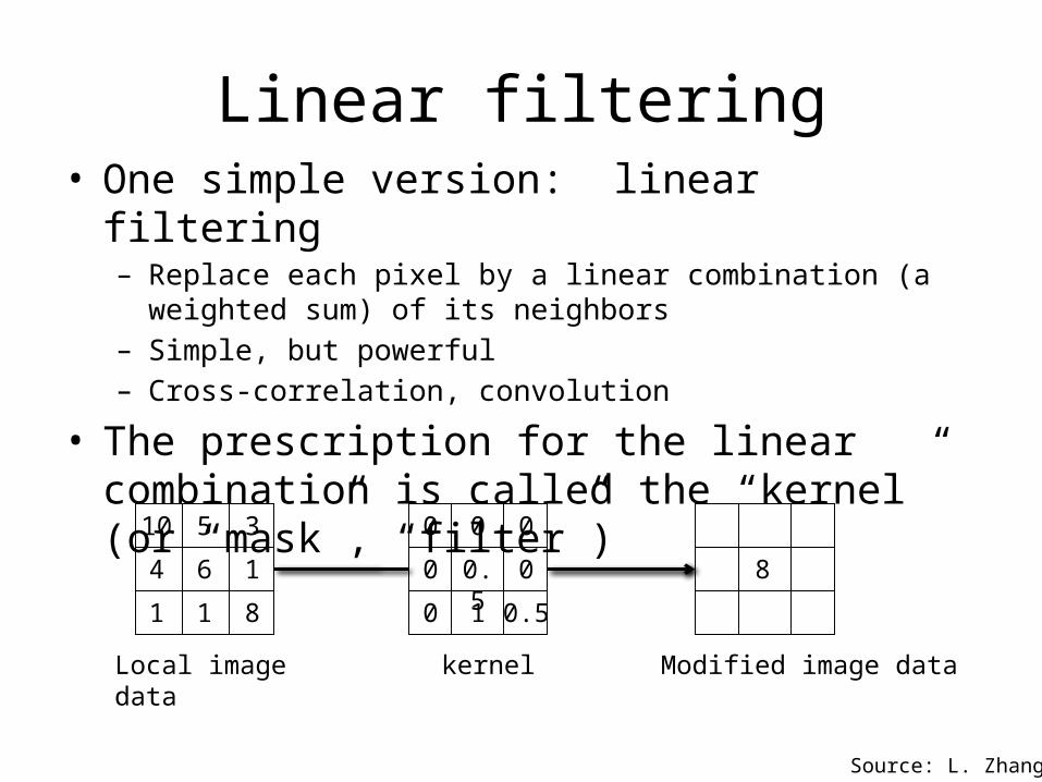
Linear filtering• One simple version: linear filtering

– Replace each pixel by a linear combination (a weighted sum) of its neighbors

– Simple, but powerful– Cross-correlation, convolution

• The prescription for the linear combination is called the “kernel” (or “mask”, “filter”)

0.5

0.5 00

10

0 00

kernel

8

Modified image data

Source: L. Zhang

Local image data

6 14

1 81

5 310

Filter Properties

• Linearity– Weighted sum of original pixel values– Use same set of weights at each point– S[f + g] = S[f] + S[g] – S[p f + q g] = p S[f] + q S[g]

• Shift-invariance– If f[m,n] g[m,n], then f[m-p,n-q] g[m-p, n-q] – The operator behaves the same everywhere

S S

Cross-correlation

This is called a cross-correlation operation:

Let be the image, be the kernel (of size 2k+1 x 2k+1), and be the output image

• Can think of as a “dot product” between local neighborhood and kernel for each pixel

Convolution• Same as cross-correlation, except that the

kernel is “flipped” (horizontally and vertically)

• Convolution is commutative and associative

This is called a convolution operation:

Convolution

Adapted from F. Durand

Pseudo-code

CS 4620 and 5625 cover topic in detail

Linear filters: examples

000

001

000

Original Shifted leftBy 1 pixel

Source: D. Lowe

* =

Convolution

• Point spread function, impulse response function

PSF of Hubble Telescope

http://aetherforce.com/wp-content/uploads/2013/10/8707342.jpg

Smoothing with box filter

Source: D. Forsyth111

111

111

Gaussian Kernel

Source: C. Rasmussen

Gaussian Kernel

0.003 0.013 0.022 0.013 0.0030.013 0.059 0.097 0.059 0.0130.022 0.097 0.159 0.097 0.0220.013 0.059 0.097 0.059 0.0130.003 0.013 0.022 0.013 0.003

5 x 5, = 1

Source: C. Rasmussen

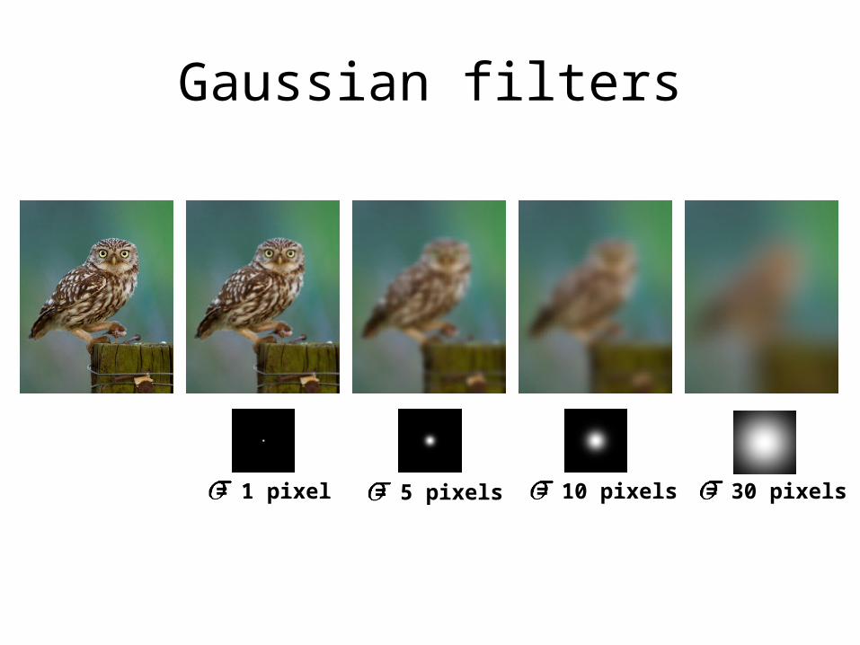
Gaussian filters

= 30 pixels= 1 pixel = 5 pixels = 10 pixels

Mean vs. Gaussian filtering

Detour: Fourier Analysis• Every signal has some frequency• Fourier analysis finds frequencies of a signal– Sum of sine/cosine waves

Source: Foley, van Dam

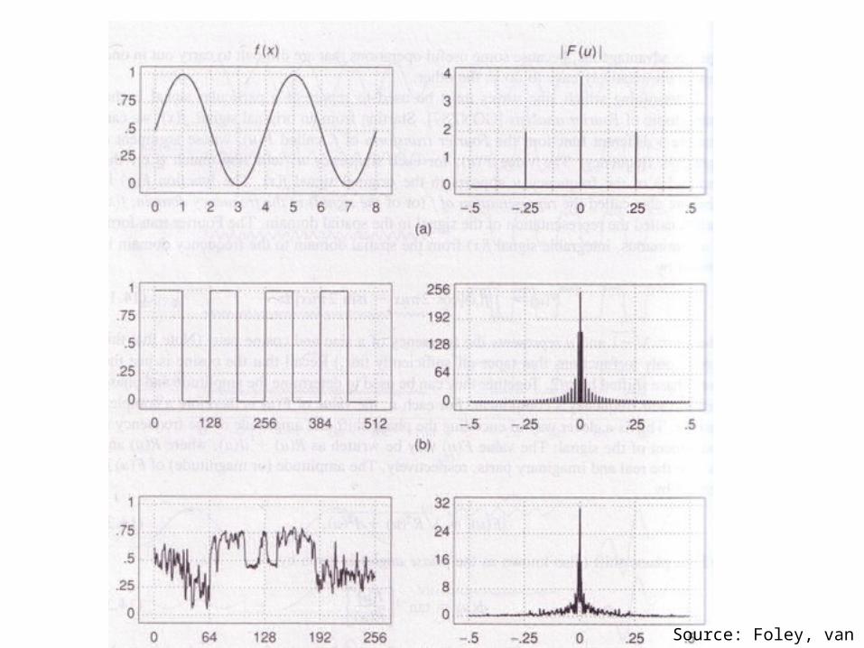
Detour: Fourier Analysis

Source: Foley, van Dam

Source: Foley, van Dam

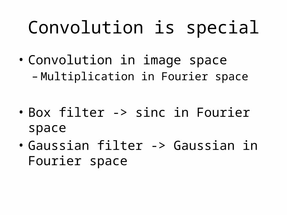
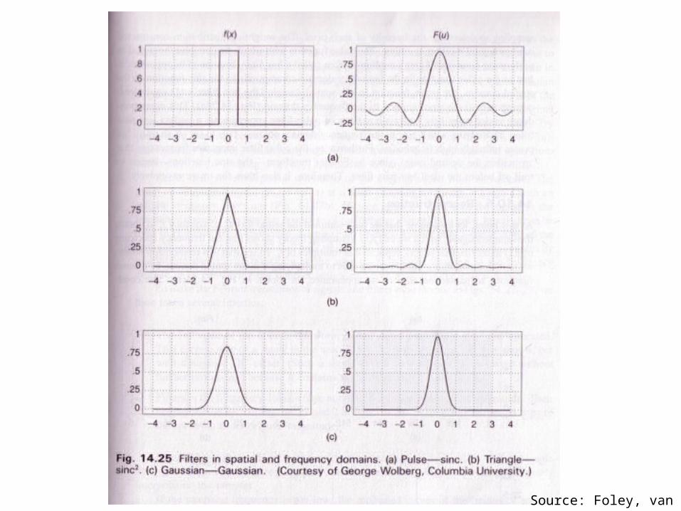
Convolution is special

• Convolution in image space– Multiplication in Fourier space

• Box filter -> sinc in Fourier space• Gaussian filter -> Gaussian in Fourier space

Low pass filtering

Source: Foley, van Dam

Gaussian filter• Removes “high-frequency” components from

the image (low-pass filter)• Convolution with self is another Gaussian

– Convolving twice with Gaussian kernel of width = convolving once with kernel of width

Source: K. Grauman

* =

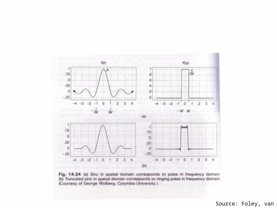
Source: Foley, van Dam

Sharpening• What does blurring take away?

original smoothed (5x5)

–

detail

=

sharpened

=

Let’s add it back:

original detail

+ α

Source: S. Lazebnik

Linear filters: examples

Original

111

111

111

000

020

000

-

Sharpening filter (accentuates edges)

Source: D. Lowe

=*

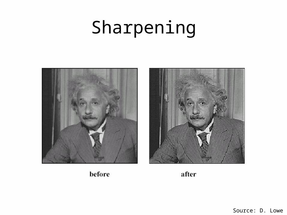
Sharpening

Source: D. Lowe

Sharpen filter

Gaussianscaled impulseLaplacian of Gaussian

imageblurredimage unit impulse

(identity)

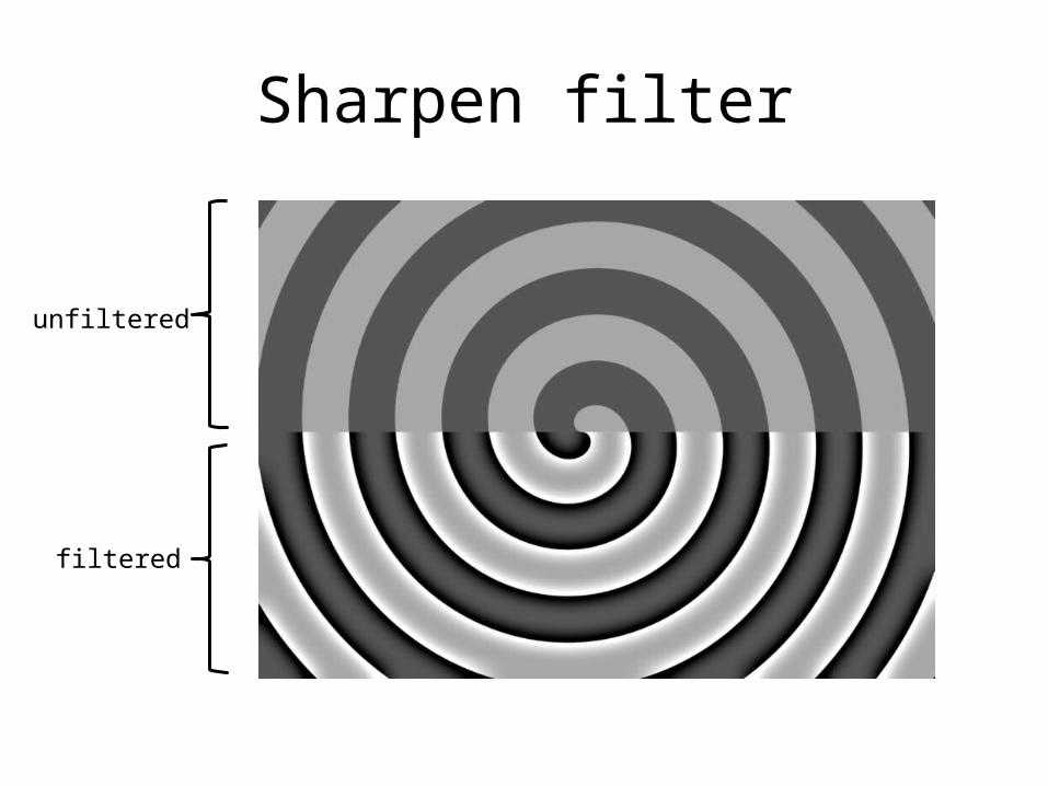
Sharpen filter

unfiltered

filtered

“Optical” Convolution

Source: http://lullaby.homepage.dk/diy-camera/bokeh.html

Bokeh: Blur in out-of-focus regions of an image.

Camera shake

*=Source: Fergus, et al. “Removing Camera Shake from a Single Photograph”, SIGGRAPH 2006