CS4670: Computer Vision Kavita Bala Lecture 8: Scale invariance.

CS4670: Computer VisionKavita Bala

Lecture 8: Scale invariance

Announcements

• HW 1 out yesterday – Due in 2 weeks on Tue 2/24– Work alone

• PA 1 demos tomorrow

Quick eigenvalue/eigenvector review

• The solution:

Once you know , you find the eigenvectors by solving

Symmetric, square matrix: eigenvectors are mutually orthogonal

The surface E(u,v) is locally approximated by a quadratic form. Let’s try to understand its shape.

Interpreting the second moment matrix

v

uMvuvuE ][),(

Invariance and covariance • We want corner locations to be invariant to photometric transformations

and covariant to geometric transformations– Invariance: image is transformed and corner locations do not change– Covariance: if we have two transformed versions of the same image,

features should be detected in corresponding locations

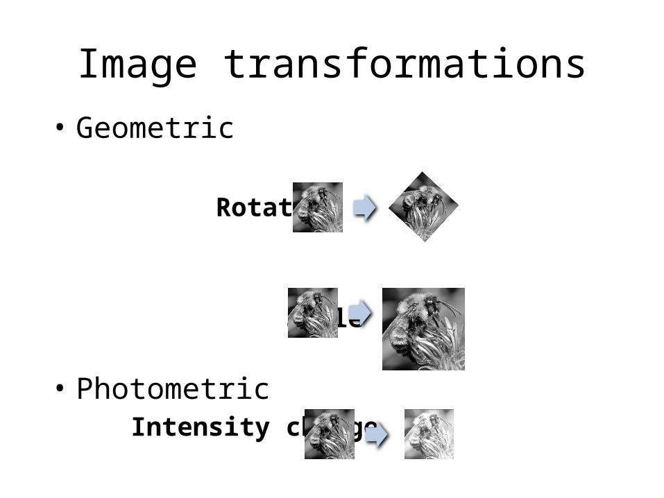
Image transformations• Geometric

Rotation

Scale

• Photometric Intensity change

Scaling

All points will be classified as edges

Corner

Corner location is not covariant to scaling!

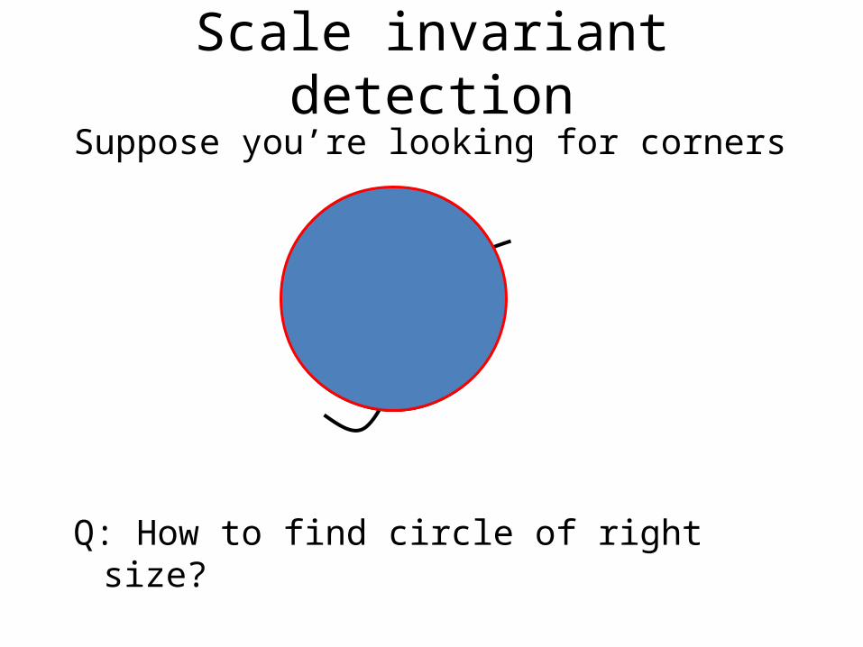
Scale invariant detectionSuppose you’re looking for corners

Q: How to find circle of right size?

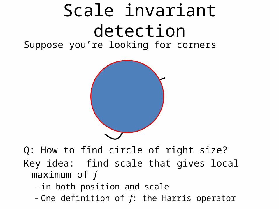
Scale invariant detectionSuppose you’re looking for corners

Q: How to find circle of right size? Key idea: find scale that gives local maximum of f

– in both position and scale– One definition of f: the Harris operator

Solution

• Design a function on the region (circle) which is “scale invariant” – i.e., the same for corresponding regions, even if at

different scales– E.g., average intensity. Same even for different

sizes

• For a point in one image, consider it as a function of region size (circle radius)

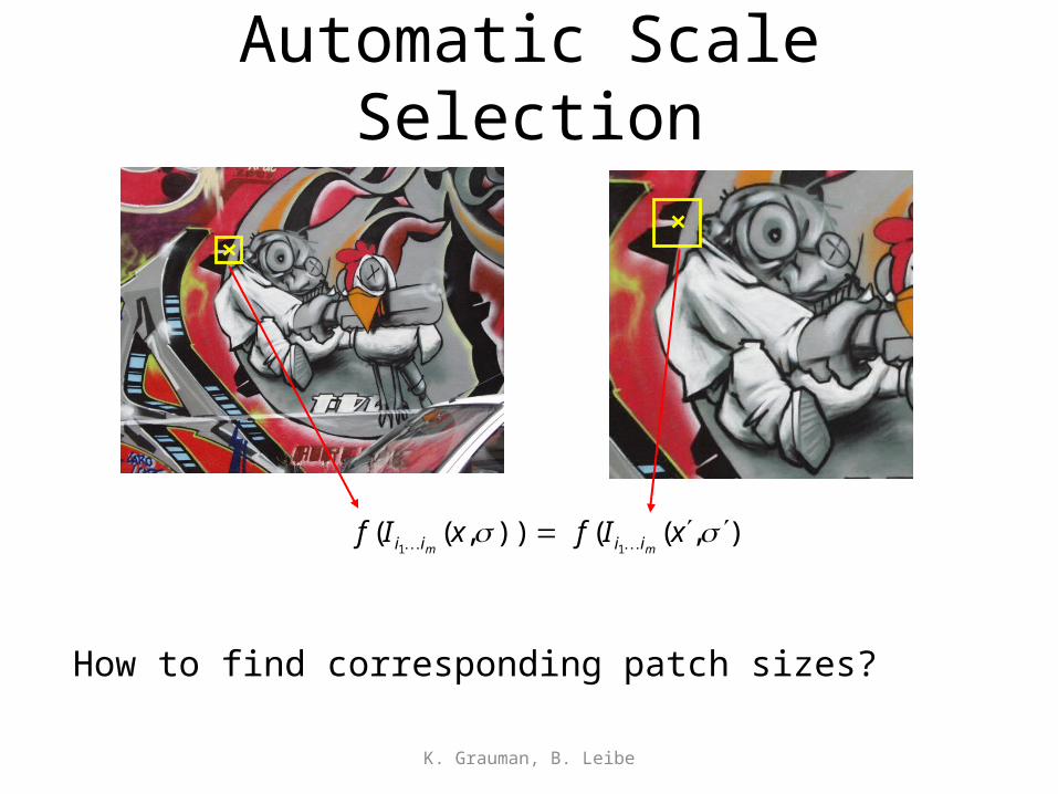
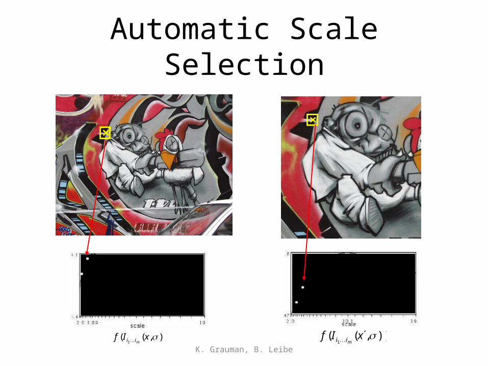
Automatic Scale Selection

K. Grauman, B. Leibe

)),(( )),((11

xIfxIfmm iiii

How to find corresponding patch sizes?

Automatic Scale Selection• Function responses for increasing scale (scale signature)

K. Grauman, B. Leibe)),((

1xIf

mii )),((1

xIfmii

Automatic Scale Selection

K. Grauman, B. Leibe)),((

1xIf

mii )),((1

xIfmii

Automatic Scale Selection

K. Grauman, B. Leibe)),((

1xIf

mii )),((1

xIfmii

Automatic Scale Selection

K. Grauman, B. Leibe)),((

1xIf

mii )),((1

xIfmii

Automatic Scale Selection

K. Grauman, B. Leibe)),((

1xIf

mii )),((1

xIfmii

Automatic Scale Selection

K. Grauman, B. Leibe)),((

1xIf

mii )),((1

xIfmii

Implementation

• Instead of computing f for larger and larger windows, we can implement using a fixed window size with a Gaussian pyramid

(sometimes need to create in-between levels, e.g. a ¾-size image)

Questions?

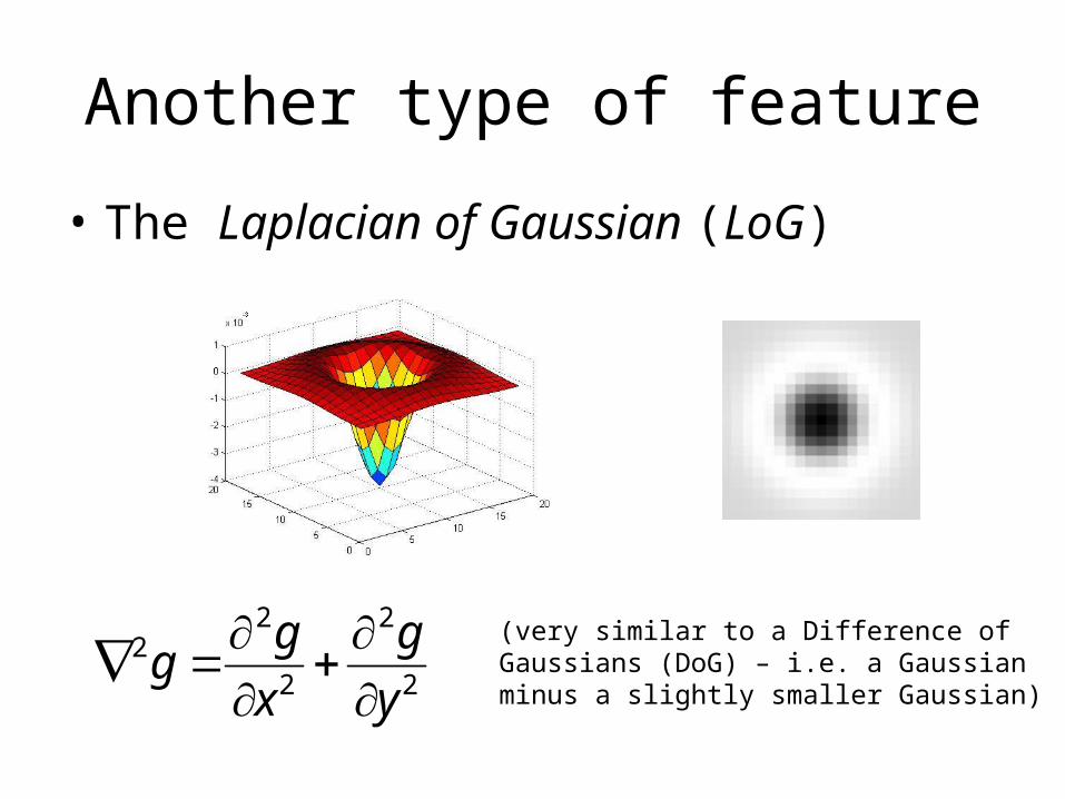
Another type of feature

• The Laplacian of Gaussian (LoG)

2

2

2

22

y

g

x

gg

(very similar to a Difference of Gaussians (DoG) – i.e. a Gaussian minus a slightly smaller Gaussian)

Laplacian of Gaussian

• “Blob” detector

• Find maxima and minima of LoG operator in space and scale

* =

maximum

minima

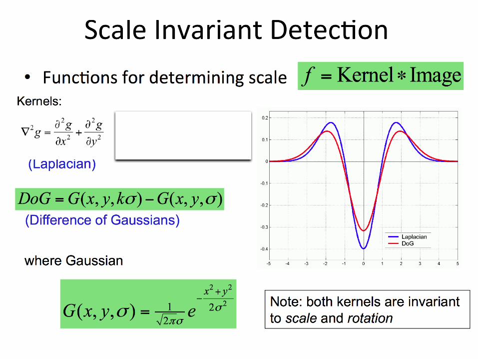
Scale selection

• At what scale does the Laplacian achieve a maximum response for a binary circle of radius r?

r

image Laplacian

Characteristic scale

• We define the characteristic scale as the scale that produces peak of Laplacian response

characteristic scale

T. Lindeberg (1998). "Feature detection with automatic scale selection." International Journal of Computer Vision 30 (2): pp 77--116.

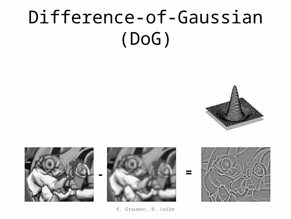
Difference-of-Gaussian (DoG)

K. Grauman, B. Leibe

- =

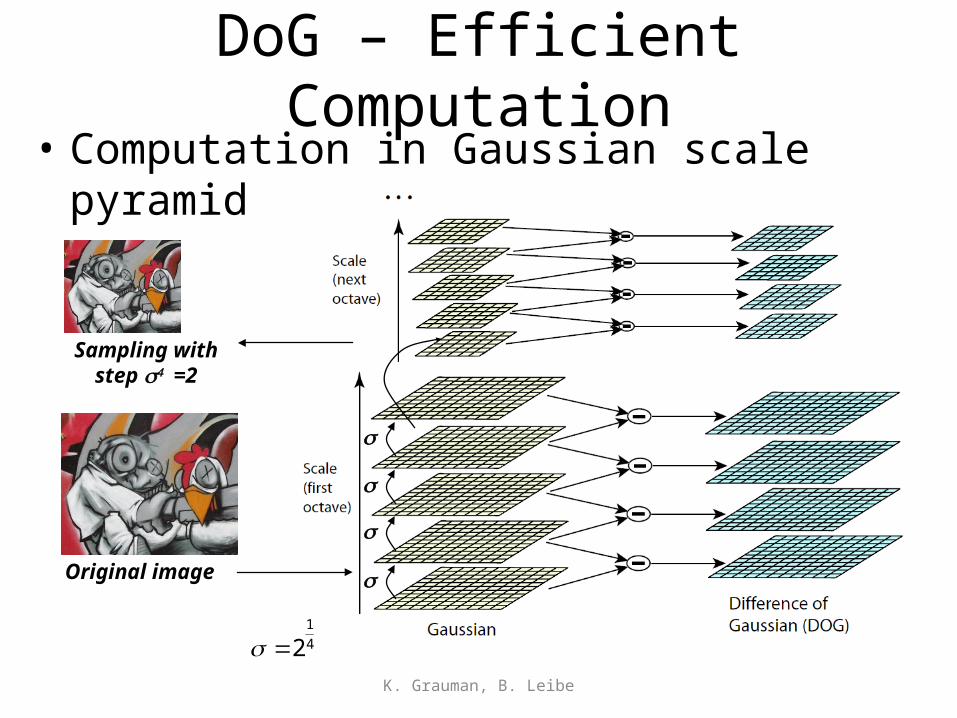
DoG – Efficient Computation• Computation in Gaussian scale pyramid

K. Grauman, B. Leibe

s

Original image

4

1

2

Sampling withstep s4 =2

s

s

s

Find local maxima in position-scale space of Difference-of-Gaussian

K. Grauman, B. Leibe

)()( yyxx LL

s

s2

s3

s4

s5

List of (x, y, s)

Results: Difference-of-Gaussian

K. Grauman, B. Leibe

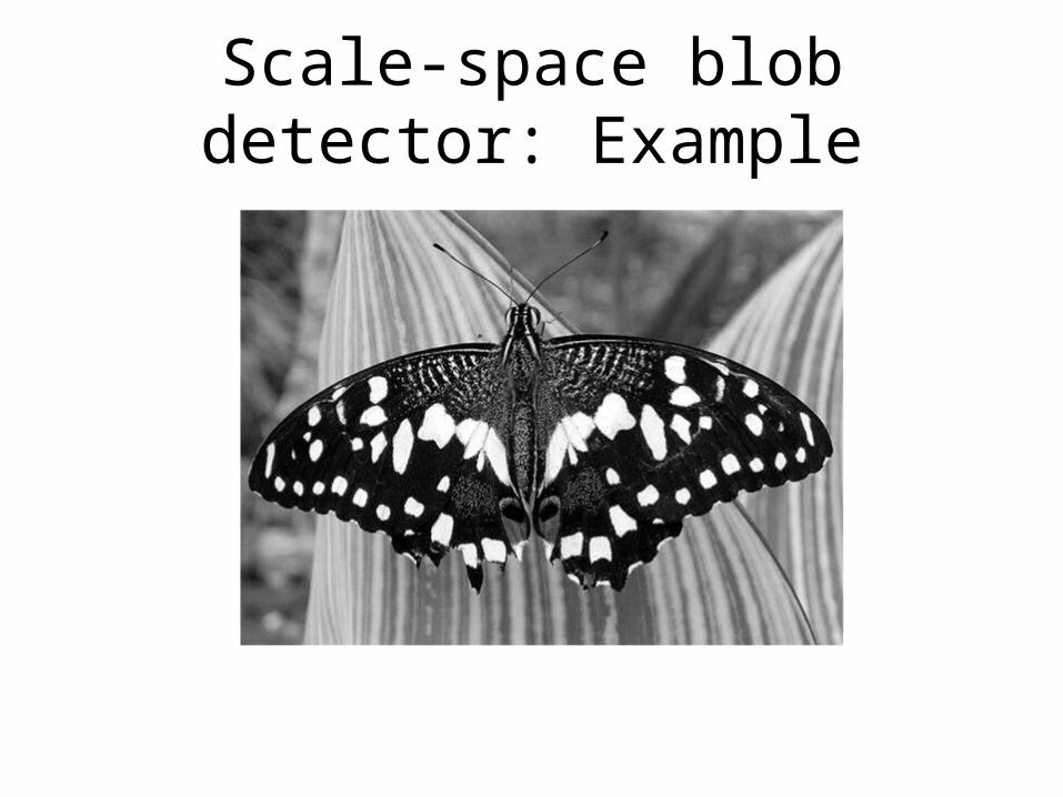
Scale-space blob detector: Example

Scale-space blob detector: Example

Scale-space blob detector: Example

Comparison of Keypoint Detectors

Tuytelaars Mikolajczyk 2008

Questions?

Feature descriptorsWe know how to detect good pointsNext question: How to match them?

Answer: Come up with a descriptor for each point, find similar descriptors between the two images

?

Feature descriptorsWe know how to detect good pointsNext question: How to match them?

Lots of possibilities (this is a popular research area)– Simple option: match square windows around the point– State of the art approach: SIFT

• David Lowe, UBC http://www.cs.ubc.ca/~lowe/keypoints/

?

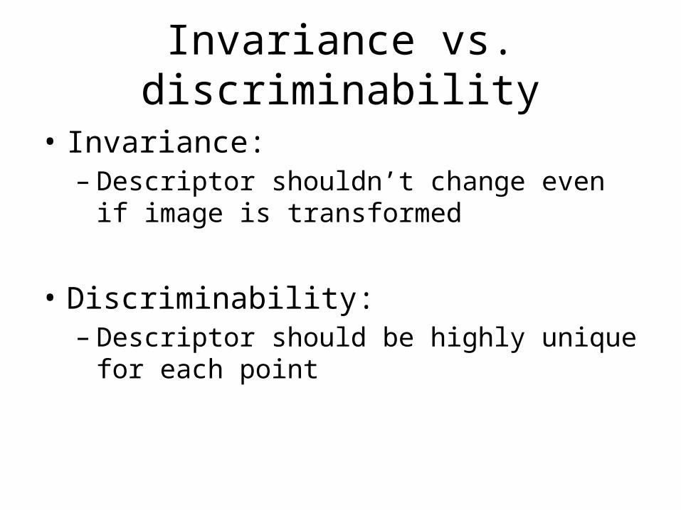
Invariance vs. discriminability

• Invariance:– Descriptor shouldn’t change even if image is

transformed

• Discriminability:– Descriptor should be highly unique for each point

Invariance

• Most feature descriptors are designed to be invariant to – Translation, 2D rotation, scale

• They can usually also handle– Limited 3D rotations (SIFT works up to about 60 degrees)– Limited affine transformations (some are fully affine invariant)– Limited illumination/contrast changes

How to achieve invariance

Need both of the following:1. Make sure your detector is invariant2. Design an invariant feature descriptor

– Simplest descriptor: a single 0• What’s this invariant to?

– Next simplest descriptor: a square window of pixels • What’s this invariant to?

– Let’s look at some better approaches…

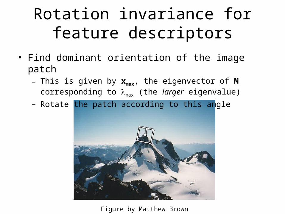
• Find dominant orientation of the image patch– This is given by xmax, the eigenvector of M corresponding to max (the

larger eigenvalue)– Rotate the patch according to this angle

Rotation invariance for feature descriptors

Figure by Matthew Brown

Take 40x40 square window around detected feature– Scale to 1/5 size (using

prefiltering)– Rotate to horizontal– Sample 8x8 square window

centered at feature– Intensity normalize the

window by subtracting the mean, dividing by the standard deviation in the window CSE 576: Computer Vision

Multiscale Oriented PatcheS descriptor

8 pixels40 pixels

Adapted from slide by Matthew Brown

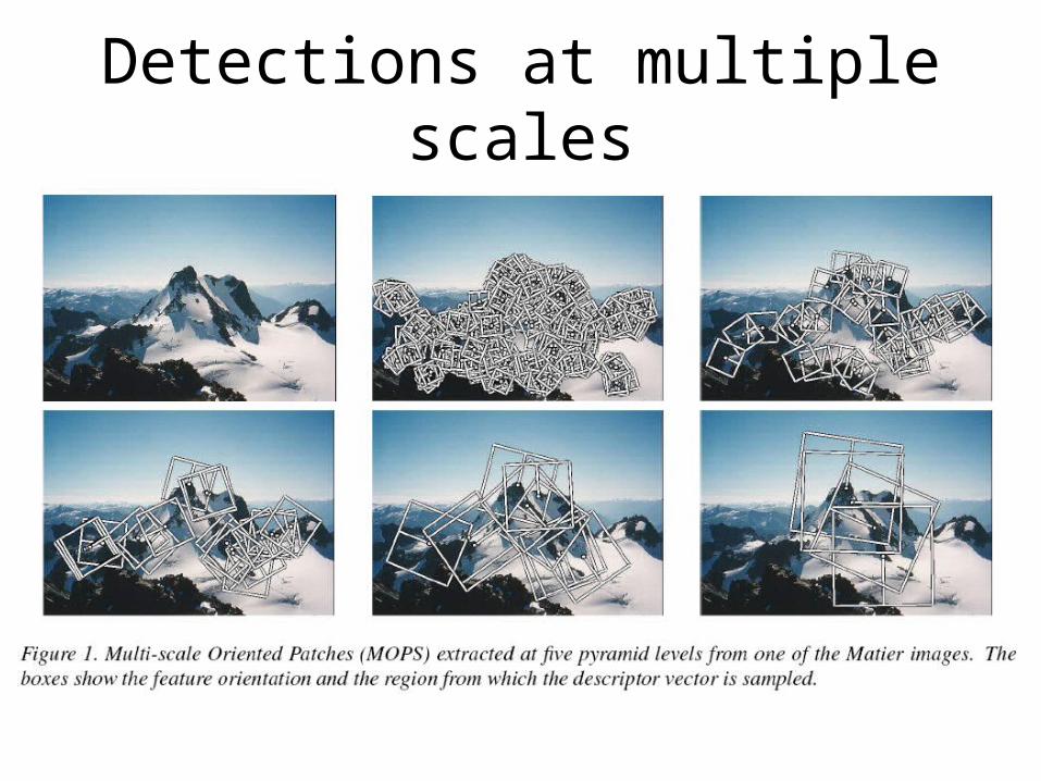
Detections at multiple scales