Learning exible models of nonlinear dynamical systemsuser.it.uu.se/~thosc112/talks/lund20170310.pdf · Learning exible models of nonlinear dynamical systems \Inspired by the Gaussian

$Page 1: Learning exible models of nonlinear dynamical systemsuser.it.uu.se/~thosc112/talks/lund20170310.pdf · Learning exible models of nonlinear dynamical systems \Inspired by the Gaussian$
Learning flexible models of nonlineardynamical systems

“Inspired by the Gaussian process and enabled by the particle filter”

Thomas SchonDivision of Systems and ControlDepartment of Information TechnologyUppsala University.

Email: [email protected],www: user.it.uu.se/~thosc112

Joint work with: Roger Frigola (independent consultant), Michael Jordan (UCBerkeley), Fredrik Lindsten (Uppsala University), Carl Rasmussen (University ofCambridge) and Andreas Svensson (Uppsala University).

Thomas Schon Department of Automatic Control, Lund University, March 10, 2017.

user.it.uu.se/~thosc112

Probabilistic modeling of dynamical systems

Probabilistic modeling allow for representing and manipulatinguncertainty in data, models, decisions and predictions.

A parametric state space model is given by:

xt+1 |xt ∼ pθ(xt+1 |xt, ut),yt |xt ∼ pθ(yt |xt, ut),

x1 ∼ pθ(x1),θ ∼ p(θ).

xt+1 = fθ(xt, ut) + vθ,t,

yt = gθ(xt, ut) + eθ,t,

x1 ∼ pθ(x1),θ ∼ p(θ).

The full probabilistic model is given by

p(x1:T , θ, y1:T ) = p(y1:T |x1:T , θ)︸︷︷︸data distribution

p(x1:T , θ)︸︷︷︸prior

1 / 25 Thomas Schon Department of Automatic Control, Lund University, March 10, 2017.

Probabilistic modeling of dynamical systems

Distribution describing a parametric nonlinear state space model:

p(x1:T , θ, y1:T ) =

T∏

t=1

p(yt |xt, θ)︸︷︷︸observation︸︷︷︸

data distribution

T−1∏

t=1

p(xt+1 |xt, θ)︸︷︷︸dynamics

p(x1 | θ)︸︷︷︸state

p(θ)︸︷︷︸param.︸︷︷︸

prior

Model = probability distribution!

Aim: Compute the posterior distribution

p(x1:T , θ | y1:T ) = p(x1:T | θ, y1:T )︸︷︷︸state

p(θ | y1:T )︸︷︷︸parameter

.


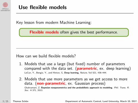
Use flexible models

Key lesson from modern Machine Learning:

Flexible models often gives the best performance.

How can we build flexible models?

1. Models that use a large (but fixed) number of parameterscompared with the data set. (parametric, ex. deep learning)LeCun, Y., Bengio, Y., and Hinton, G. Deep learning, Nature, Vol 521, 436–444.

2. Models that use more parameters as we get access to moredata. (non-parametric, ex. Gaussian process)Ghahramani, Z. Bayesian nonparametrics and the probabilistic approach to modeling. Phil. Trans. R.Soc. A 371, 2013.


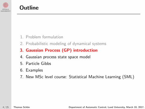
Outline

1. Problem formulation

2. Probabilistic modeling of dynamical systems

3. Gaussian Process (GP) introduction

4. Gaussian process state space model

5. Particle Gibbs

6. Examples

7. New MSc level course: Statistical Machine Learning (SML)


An abstract idea

In probabilistic linear regression

yi = βTxi︸︷︷︸f(x)

+εi, εi ∼ N (0, σ2),

we place a prior on β, β ∼ N (0, σ2Ip).

(Abstract) idea: What if we instead place a prior directlyon the function f(·)

f ∼ p(f)

and look for p(f |y) rather than p(β |y)?!


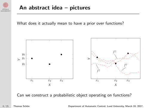
An abstract idea – pictures

What does it actually mean to have a prior over functions?

Chapter 3

Gaussian Processes

The Gaussian process (GP) is a nonparametric and probabilistic model also for nonlinear relationships. Herewe will use it for the purpose of regression. The nonparametric nature means that the GP does not rely onany parametric model assumption—instead the GP is flexible with the capability to adapt the model complexityas more data arrives. This means that the training data is not summarized by a few parameters (as for linearregression) but is part of the model (as for k-NN). The probabilistic nature of the GP provides a structured way ofrepresenting and reasoning about the uncertainty that is present both in the model itself and the measured data.

3.1 Constructing the Gaussian process

x1 x2 x3

y1

y2

y3

X

Y

(a) The data {xi, yi}3i=1, which we want to have a model for.

x1 x2 x3

f?

f?

f?

XY

(b) We assume there exists some function f , which describesthe data as yi = f(xi) + εi.

Figure 3.1: Some data are shown in the left panel, which would not be well explained by a linear model. Instead, we assumethere exists some function f (right panel), about which we are going to reason by making use of the Gaussian process.

Assume that we want to fit a model to some training data T = {xi, yi}3i=1, as we show in Figure 3.1a.We could make use of linear regression, but even from just these three data points it looks like a simple linearregression model Y = β0 + β1X + ε might be inadequate. Using nonlinear transformations of the input X(polynomials, say) is a possibility, but it can be hard to know what transformations to consider in practice. Instead,we try a different approach in specifying a model. Instead of assuming that we have a linear function, let us justsay there exists some (possibly non-linear) function f , which describes the data points as yi = f(xi) + εi, asillustrated by Figure 3.1b.

For two different input values x and x′, the unknown function f takes some output values f(x) and f(x′),respectively. Let us now reason probabilistically about this unknown f , by assuming that f(x) and f(x′) are

14

Can we construct a probabilistic object operating on functions?


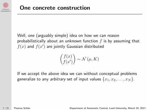
One concrete construction

Well, one (arguably simple) idea on how we can reasonprobabilistically about an unknown function f is by assuming thatf(x) and f(x′) are jointly Gaussian distributed

(f(x)f(x′)

)∼ N (µ,K)

If we accept the above idea we can without conceptual problemsgeneralize to any arbitrary set of input values {x1, x2, . . . , xN}.


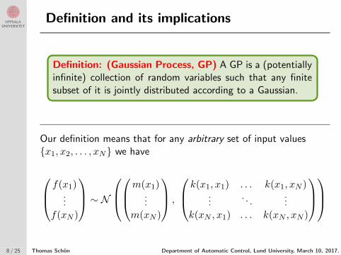
Definition and its implications

Definition: (Gaussian Process, GP) A GP is a (potentiallyinfinite) collection of random variables such that any finitesubset of it is jointly distributed according to a Gaussian.

Our definition means that for any arbitrary set of input values{x1, x2, . . . , xN} we have

f(x1)

...f(xN )

∼ N

m(x1)

...m(xN )

,

k(x1, x1) . . . k(x1, xN )

.... . .

...k(xN , x1) . . . k(xN , xN )


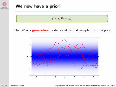
We now have a prior!

f ∼ GP(m, k)

The GP is a generative model so let us first sample from the prior.


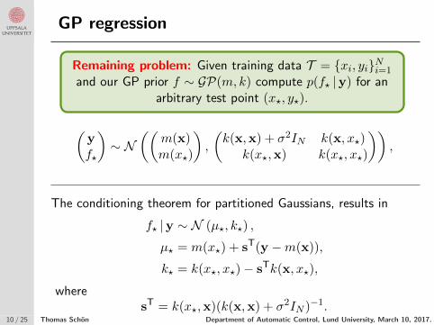
GP regression

Remaining problem: Given training data T = {xi, yi}Ni=1

and our GP prior f ∼ GP(m, k) compute p(f? |y) for anarbitrary test point (x?, y?).

(yf?

)∼ N

((m(x)m(x?)

),

(k(x,x) + σ2IN k(x, x?)

k(x?,x) k(x?, x?)

)),

The conditioning theorem for partitioned Gaussians, results in

f? |y ∼ N (µ?, k?) ,

µ? = m(x?) + sT(y −m(x)),

k? = k(x?, x?)− sTk(x, x?),

wheresT = k(x?,x)(k(x,x) + σ2IN )−1.


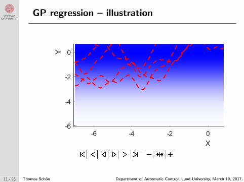
GP regression – illustration


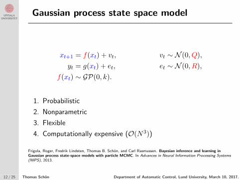
Gaussian process state space model

xt+1 = f(xt) + vt, vt ∼ N (0, Q),

yt = g(xt) + et, et ∼ N (0, R),

f(xt) ∼ GP(0, k).

1. Probabilistic

2. Nonparametric

3. Flexible

4. Computationally expensive (O(N3))

Frigola, Roger, Fredrik Lindsten, Thomas B. Schon, and Carl Rasmussen. Bayesian inference and learning inGaussian process state-space models with particle MCMC. In Advances in Neural Information Processing Systems(NIPS), 2013.


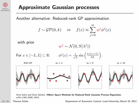
Approximate Gaussian processes

Popular alternative: Sparse approximations (inducing variables)

X∗

f ∗

Data

X∗

f ∗

Inducing variablesData

J. Quinonero-Candela and C. E. Rasmussen. A unifying view of sparse approximate Gaussian process regression.Journal of Machine Learning Research, 6:1935–1959, 12 2005.


Approximate Gaussian processes

Another alternative: Reduced-rank GP approximation

f ∼ GP(0, k) ⇔ f(x) ≈m∑

j=0

wjφj(x)

with priorwj ∼ N (0, S(λj))

For x ∈ [−L,L] ⊂ R: φj(x) = 1√L

sin(πj(x+L)

2L

).

m = 4Full GP m = 16m = 9

Arno Solin and Simo Sarkka. Hilbert Space Methods for Reduced-Rank Gaussian Process Regression.arXiv:1401.5508, 2014.


Computationally feasible GP-SSM

Original formulation:

xt+1 = f(xt) + vt, vt ∼ N (0, Q),

yt = g(xt) + et, et ∼ N (0, R),

f(xt) ∼ GP(0, k).

Formulation using the reduced-rank GP approximation:

xt+1 =

m∑

j=0

wjφj(xt) + vt, vt ∼ N (0, Q),

yt = g(xt) + et, et ∼ N (0, R),

wj ∼ N (0, S(λj)).


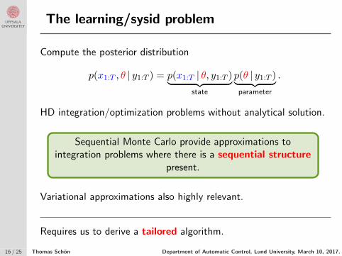
The learning/sysid problem

Compute the posterior distribution

p(x1:T , θ | y1:T ) = p(x1:T | θ, y1:T )︸︷︷︸state

p(θ | y1:T )︸︷︷︸parameter

.

HD integration/optimization problems without analytical solution.

Sequential Monte Carlo provide approximations tointegration problems where there is a sequential structure

present.

Variational approximations also highly relevant.

Requires us to derive a tailored algorithm.


Outline

1. Problem formulation

2. Probabilistic modeling of dynamical systems

3. Gaussian Process (GP) introduction

4. Gaussian process state space model

5. Particle Gibbs

6. Examples

7. New MSc level course: Statistical Machine Learning (SML)


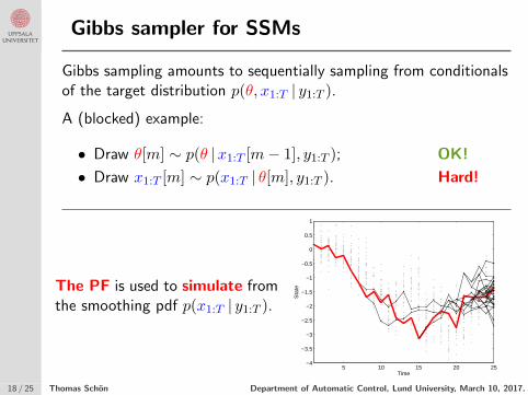
Gibbs sampler for SSMs

Gibbs sampling amounts to sequentially sampling from conditionalsof the target distribution p(θ, x1:T | y1:T ).

A (blocked) example:

• Draw θ[m] ∼ p(θ |x1:T [m− 1], y1:T ); OK!

• Draw x1:T [m] ∼ p(x1:T | θ[m], y1:T ). Hard!

The PF is used to simulate fromthe smoothing pdf p(x1:T | y1:T ).

5 10 15 20 25−4

−3.5

−3

−2.5

−2

−1.5

−1

−0.5

0

0.5

1

Time

Sta

te


Problems and a solution

Problems with this approach,• Based on a PF ⇒ approximate sample.

• Does not leave p(x1:T | θ, y1:T ) invariant!

• Relies on large N to be successful.

• A lot of wasted computations.

To get around these problems,

Use a conditional particle filter (CPF). One pre-specifiedreference trajectory is retained throughout the sampler.

Christophe Andrieu, Arnaud Doucet and Roman Holenstein, Particle Markov chain Monte Carlo methods, Journalof the Royal Statistical Society: Series B, 72:269-342, 2010.

Fredrik Lindsten, Michael I. Jordan and Thomas B. Schon, Particle Gibbs with ancestor sampling. Journal ofMachine Learning Research, 15(1):2145–2184, 2014.


CPF-AS – intuition

Let x′1:T = (x′1, . . . , x′T ) be a fixed reference trajectory.

• At each time t, sample N − 1 particles in the standard way.

• Set the N th particle deterministically: xNt = x′t.

• Generate an artificial history for xNt by ancestor sampling.

“

The CPF-AS causes us to degenerate to something that is verydifferent from the reference trajectory, resulting in better mixing.


Toy example

xt+1 = 10sinc(xt

7

)+ vt vt ∼ N (0, 4)

yt = xt + et (known) et ∼ N (0, 4)

T = 40,m = 40

Posterior model uncertaintyLearned modelTrue state transition functionState samples underlying dataBasis functions

No prior

−30 −20 −10 0 10 20 30−10

010

xt

xt+

1

With (GP-inspired) prior

−30 −20 −10 0 10 20 30−10

010

xt

xt+

1

Full posterior

−30 −20 −10 0 10 20 30−10

010

xtxt+

1


Narendra-Li Benchmark

x1t+1 =

(x1t

1+(x1t )

2 + 1)sin(x2

t )

x2t+1 =x2

t cos(x2t ) + x1

t exp(− (x1

t )2+(x2

t )2

8

)+ (ut)

3

1+(ut)2+0.5 cos(x1t+x2

t )

yt =x1t

1+0.5 sin(x2t )

+x2t

1+0.5 sin(x1t )

+ et

Method RMSE T

This 0.06 2 000Roll et al. 0.43 50 000Stenman et al. 0.46 50 000Xu et al. (AHH) 0.31 2 000Xu et al. (MARS) 0.49 2 000

J. Roll, A. Nazin, and L. Ljung. Nonlinear system identification via direct weight optimization. Automatica,41(3):475–490, 2005.

A. Stenman. Model on demand: Algorithms, analysis and applications. PhD thesis, Linkoping University, 1999.

J. Xu, X. Huang, and S. Wang. Adaptive hinging hyperplanes and its applications in dynamic systemidentification. Automatica, 45(10):2325–2332, 2009.


Regularization in nonlinear state spaces

m = 6

m = 100

m = 100+ regularization

Data

−3 −2 −1 0 1 2 3

−2

02

−2

02

−2

02

x𝑡

x𝑡+

1=

f(x

𝑡)

True functionStandard deviation of 𝑤t

Identified functionEstimated standard deviation of 𝑤t

Fig. 1. The first example, with three different settings: 𝑚 = 6 basisfunctions (top), 𝑚 = 100 basis functions (middle) and 𝑚 = 100 basisfunctions with regularization (bottom). The model with 𝑚 = 6 is not flexibleenough to describe the ‘steep’ part of 𝑓 , but results in a sensible, albeit notperfect, model. The second model is very flexible with its 101 parameters, andbecomes a typical case of over-fitting to the data points (cf. the distributionof the data at the very bottom), causing numerical problems and a uselessmodel. The regularization in the third case is a clear remedy to this problem,still maintaining the high flexibility of the model.

A natural question is indeed how to choose the prior preci-sion 𝑃 . As stated by [12], the optimal choice (in terms of meansquare error) is 𝑃−1

opt = E[[𝜔(1) · · · 𝜔(𝑚)]T[𝜔(1) · · · 𝜔(𝑚)]

],

if we think of 𝜔(1), . . . , 𝜔(𝑚) as being random variables.As an example, with the natural assumption of 𝑓𝑥(·) beingsmooth, the diagonal elements of 𝑃 should be larger withincreasing order of the Fourier basis functions. The specialcase of assuming 𝑓𝑥(·) to be a sample from a Gaussian processis addressed by [14].

Other regularization schemes, such as 𝐿1, are possible butwill not result in closed-form expressions such as (9).

C. Computational aspects

Let 𝑁 denote the number of particles in the CPF-AS, 𝑚 thenumer of terms used in the basis function expansion, 𝑇 thenumber of data points and 𝐾 the numer of iterations used inAlgorithm 2. The computational load is then 𝒪(𝑚𝑇𝐾𝑁) +𝒪(𝑚3). In practice, 𝑁 and 𝑚 can be chosen fairly small (e.g.,𝑁 = 5 and 𝑚 = 10 for a 1D model).

D. Convergence

The convergence properties of PSAEM are not yet fullyunderstood, but it can under certain assumptions be shownto converge to a stationary point of 𝑝𝜃(𝑢1:𝑇 , 𝑦1:𝑇 ) by [17,Theorem 1]. We have not experienced practical problems withthe convergence, although it is sensitive to initialization whenthe dimension of 𝜃 is large (e.g., 1 000 parameters).

TABLE IRESULTS FOR THE HAMMERSTEIN-WIENER BENCHMARK

Experiment with 𝑇 = 2000Mean simulation error 0.0005 V

Standard deviation of simulation error 0.020 VRMS simulation error 0.020 V

Run time 13 min

IV. NUMERICAL EXAMPLES

We demonstrate our proposed method on a series of numer-ical examples. The source code is available via the web siteof the first author.

A. Simulated example

As a first simple numerical example, consider an au-tonomous system (i.e., no 𝑢𝑡) defined by

𝑥𝑡+1 =−10𝑥𝑡

1 + 3𝑥2𝑡

+ 𝑤𝑡, 𝑦𝑡 = 𝑥𝑡 + 𝑒𝑡, (10)

where 𝑤𝑡 ∼ 𝒩 (0, 0.1) and 𝑒𝑡 ∼ 𝒩 (0, 0.5). We identify 𝑓(·)and 𝑄 from 𝑇 = 1000 simulated measurements 𝑦1:𝑇 , whileassuming 𝑔(·) and 𝑅 to be known. We consider three differentsettings with 𝑚 = 6 basis functions, 𝑚 = 100 basis functionsand 𝑚 = 100 basis functions with regularization, respectively,all using the Fourier basis. To encode the a priori assumptionof 𝑓(·) being a smooth function, we choose the regularizationas a Gaussian prior of 𝑤𝑘 with standard deviation inverselyproportional to 𝑘. The results are shown in Figure 1, wherethe over-fitting problem for 𝑚 = 100, and how regularizationhelps, is apparent.

B. Hammerstein-Wiener benchmark

To illustrate how to adapt our approach to problems witha given structure, we apply it to the real-data Hammerstein-Wiener system identification benchmark by [20]. We will usea subset with 2 000 data points from the original data set forestimation. Based on the domain knowledge provided by [20](two third order linear systems in a cascade with a staticnonlinearity between), we identify a model with the structure

[𝑥1𝑡+1

𝑥2𝑡+1

𝑥3𝑡+1

]= 𝐴1

[𝑥1𝑡

𝑥2𝑡

𝑥3𝑡

]+𝐵𝑢𝑡, (11a)

[𝑥4𝑡+1

𝑥5𝑡+1

𝑥6𝑡+1

]= 𝐴2

[𝑥4𝑡

𝑥5𝑡

𝑥6𝑡

]+

[Σ𝑘𝜔

(𝑘)𝜑(𝑘)(𝑥3𝑡 )

0

0

], (11b)

𝑦𝑡 = 𝐶 [ 𝑥4𝑡 𝑥5

𝑡 𝑥6𝑡 ] , (11c)

where the superindex on the state denotes a particular com-ponent of the state vector. Furthermore, we have omittedall noise terms for notational brevity. There is only onenonlinear function, but the linear parts can be seen as thespecial case where {𝜑(𝑘)(𝑥)}𝑚𝑘=1 = {𝑥}, which can directlybe incorporated into the presented framework.

We present the results in Table I (all metrics are with respectto the evaluation data from the original data set). We refer to[21] for a thorough evaluation of alternative methods.

Results in a flexible non-parametric model where theGP prior on f takes on therole of a regularizer.

Provides a data-driven way oftuning the model flexibility.

Toy example:

xt+1 = −10xt

1 + 3x2t+ vt,

yt = xt + et.

For all details on the new model and more examples, seeAndreas Svensson and Thomas B. Schon. A flexible state space model for learning nonlinear dynamical systems,Automatica, 2017. (Accepted for publication)


ASSEMBLE project

Aim: Automate probabilistic modeling of dynamicalsystems (and their surroundings) via a formallydefined probabilistic modeling language.

Probabilistic Model Compiler

Application Model

Inference Methods

Application Specific Machine Learning

Solution

Probabilistic Modeling Research

Inference Methods Research

Modeling Language Research

Demonstrators Smart Meters (Greenely) Cell Tracking (Karolinska Institute) Energy-Aware Computing Container Crane Automation (ABB) Smart Automotive Safety (Autoliv)

- Improved modeling techniques - Improved inference methods - Enhanced modeling language

Feedback from demonstrators enables:

We will create a market place for inference and learningalgorithms and probabilistic model libraries for dynamical systemsand their environments.


Conclusions

Constructed a Gaussian process state space model.

Prior = regularization, helping the model to generalizewithout sacrificing the flexibility offered by the basis

function expansion.

A flexible model often gives the best performance.

The resulting learning problems require approximations.

Huge need for automation (ASSEMBLE project).

Hosting the SMC workshop in Uppsala, Aug. 30-Sep. 1, 2017.Preliminary (for now) web site:

http://www.it.uu.se/conferences/smc2017


http://www.it.uu.se/conferences/smc2017

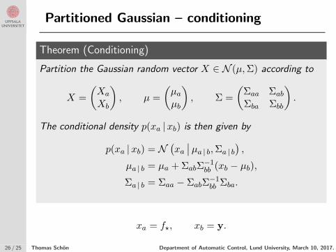
Partitioned Gaussian – conditioning

Theorem (Conditioning)

Partition the Gaussian random vector X ∈ N (µ,Σ) according to

X =

(Xa

Xb

), µ =

(µaµb

), Σ =

(Σaa Σab

Σba Σbb

).

The conditional density p(xa |xb) is then given by

p(xa |xb) = N(xa∣∣µa | b,Σa | b

),

µa | b = µa + ΣabΣ−1bb (xb − µb),

Σa | b = Σaa − ΣabΣ−1bb Σba.

xa = f?, xb = y.


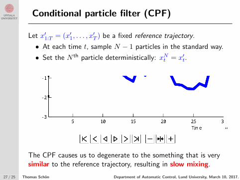
Conditional particle filter (CPF)

Let x′1:T = (x′1, . . . , x′T ) be a fixed reference trajectory.

• At each time t, sample N − 1 particles in the standard way.

• Set the N th particle deterministically: xNt = x′t.

“

The CPF causes us to degenerate to the something that is verysimilar to the reference trajectory, resulting in slow mixing.


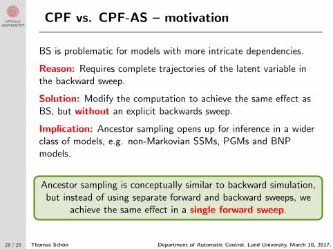
CPF vs. CPF-AS – motivation

BS is problematic for models with more intricate dependencies.

Reason: Requires complete trajectories of the latent variable inthe backward sweep.

Solution: Modify the computation to achieve the same effect asBS, but without an explicit backwards sweep.

Implication: Ancestor sampling opens up for inference in a widerclass of models, e.g. non-Markovian SSMs, PGMs and BNPmodels.

Ancestor sampling is conceptually similar to backward simulation,but instead of using separate forward and backward sweeps, we

achieve the same effect in a single forward sweep.


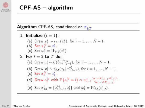
CPF-AS – algorithm

Algorithm CPF-AS, conditioned on x′1:T

1. Initialize (t = 1):(a) Draw xi1 ∼ rθ,1(xi1), for i = 1, . . . , N − 1.(b) Set xN1 = x′1.(c) Set wi1 = Wθ,1(xi1).

2. For t = 2 to T do:(a) Draw ait ∼ C({wjt}Nj=1), for i = 1, . . . , N − 1.

(b) Draw xit ∼ rθ,t(xt |xait1:t−1), for i = 1, . . . , N − 1.

(c) Set xNt = x′t.

(d) Draw aNt with P(aNt = i

)∝ wit−1

γθ,T (xi1:t−1,x

′t:T )

γθ,t−1(xi1:t−1).

(e) Set xi1:t = {xait

1:t−1, xit} and wit = Wθ,t(x

i1:t).


Learning exible models of nonlinear dynamical systemsuser.it.uu.se/~thosc112/talks/lund20170310.pdf · Learning exible models of nonlinear dynamical systems \Inspired by the Gaussian

Documents