Welcome message from author
This document is posted to help you gain knowledge. Please leave a comment to let me know what you think about it! Share it to your friends and learn new things together.
Transcript
Texts in Applied Mathematics 2
Editors
J.E. MarsdenL. SirovichS.S. Antman
Advisors
G. IoossP. HolmesD. BarkleyM. DellnitzP. Newton

This page intentionally left blank
Stephen Wiggins
Introduction toApplied Nonlinear DynamicalSystems and Chaos
Second Edition
With 250 Figures
Stephen WigginsSchool of MathematicsUniversity of BristolClifton, Bristol BS8 [email protected]
Series Editors
J.E. Marsden L. SirovichControl and Dynamical Systems, 107–81 Division of Applied MathematicsCalifornia Institute of Technology Brown UniversityPasadena, CA 91125 Providence, RI 02912USA [email protected] [email protected]
S.S. AntmanDepartment of MathematicsandInstitute for Physical Scienceand Technology
University of MarylandCollege Park, MD [email protected]
Mathematics Subject Classification (2000): 58Fxx, 34Cxx, 70Kxx
Library of Congress Cataloging-in-Publication DataWiggins, Stephen.
Introduction to applied nonlinear dynamical systems and chaos / Stephen Wiggins. — 2nd ed.p. cm. — (Texts in applied mathematics ; 2)
Includes bibliographical references and index.ISBN 0-387-00177-8 (alk. paper)1. Differentiable dynamical systems. 2. Nonlinear theories. 3. Chaotic behavior in
systems. I. Title. II. Texts in applied mathematics ; 2.QA614.8.W544 2003003′.85—dc21 2002042742
ISBN 0-387-00177-8 Printed on acid-free paper.
2003, 1990 Springer-Verlag New York, Inc.All rights reserved. This work may not be translated or copied in whole or in part without the writtenpermission of the publisher (Springer-Verlag New York, Inc., 175 Fifth Avenue, New York, NY 10010,USA), except for brief excerpts in connection with reviews or scholarly analysis. Use in connection withany form of information storage and retrieval, electronic adaptation, computer software, or by similar ordissimilar methodology now known or hereafter developed is forbidden.The use in this publication of trade names, trademarks, service marks, and similar terms, even if they arenot identified as such, is not to be taken as an expression of opinion as to whether or not they are subjectto proprietary rights.
Printed in the United States of America.
9 8 7 6 5 4 3 2 1 SPIN 10901182
www.springer-ny.com
Springer-Verlag New York Berlin HeidelbergA member of BertelsmannSpringer Science+Business Media GmbH
Series Preface
Mathematics is playing an ever more important role in the physical andbiological sciences, provoking a blurring of boundaries between scientificdisciplines and a resurgence of interest in the modern as well as the classicaltechniques of applied mathematics. This renewal of interest, both in re-search and teaching, has led to the establishment of the series Texts inApplied Mathematics (TAM).The development of new courses is a natural consequence of a high level
of excitement on the research frontier as newer techniques, such as numeri-cal and symbolic computer systems, dynamical systems, and chaos, mixwith and reinforce the traditional methods of applied mathematics. Thus,the purpose of this textbook series is to meet the current and future needsof these advances and to encourage the teaching of new courses.TAM will publish textbooks suitable for use in advanced undergraduate
and beginning graduate courses, and will complement the Applied Mathe-matical Sciences (AMS) series, which will focus on advanced textbooks andresearch-level monographs.
Pasadena, California J.E. MarsdenProvidence, Rhode Island L. SirovichCollege Park, Maryland S.S. Antman

This page intentionally left blank
Preface to the Second Edition
This edition contains a significant amount of new material. The main rea-son for this is that the subject of applied dynamical systems theory hasseen explosive growth and expansion throughout the 1990s. Consequently,a student needs a much larger toolbox today in order to begin research onsignificant problems.
I also try to emphasize a broader and more unified point of view. Mygoal is to treat dissipative and conservative dynamics, discrete and con-tinuous time systems, and local and global behavior, as much as possible,on the same footing. Many textbooks tend to treat most of these issuesseparately (e.g., dissipative, discrete time, local dynamics; global dynamicsof continuous time conservative systems, etc.). However, in research onegenerally needs to have an understanding of each of these areas, and theirinter-relations. For example, in studying a conservative continuous timesystem, one might study periodic orbits and their stability by passing to aPoincare map (discrete time). The question of how stability may be affectedby dissipative perturbations may naturally arise. Passage to the Poincaremap renders the study of periodic orbits a local problem (i.e., they are fixedpoints of the Poincare map), but their manifestation in the continuous timeproblem may have global implications. An ability to put together a “bigpicture” from many (seemingly) disparate pieces of information is crucialfor the successful analysis of nonlinear dynamical systems.
This edition has seen a major restructuring with respect to the firstedition in terms of the organization of the chapters into smaller units witha single, common theme, and the exercises relevant to each chapter nowbeing given at the end of the respective chapter.
The bulk of the material in this book can be covered in three ten weekterms. This is an ambitious program, and requires relegating some of thematerial to background reading (described below). My goal was to have thenecessary background material side-by-side with the material that I wouldlecture on. This tends to be more demanding on the student, but with theright guidance, it also tends to be more rewarding and lead to a deeperunderstanding and appreciation of the subject.
The mathematical prerequisites for the course are really not great; ele-mentary analysis, multivariable calculus, and linear algebra are sufficient.In reality, this may not be enough on its own. A successful understandingof applied dynamical systems theory requires the students to have an inte-

viii Preface to the Second Edition
grated knowledge of these prerequisites in the sense that they can fluidlymanipulate and use the ideas between the subjects. This means they mustpossess the quality often referred to as “mathematical maturity.” A studyof dynamical systems theory can be a good way to obtain this. In addi-tion, an ordinary differential equations course from the geometric point ofview (e.g., the material in the books of Arnold [1973] or Hirsch and Smale[1974]) would be ideal.
Chapters 1-17 form the core of the first term material. It provides stu-dents with the basic concepts and tools for the study of dynamical systemstheory. I tend to cover chapters 7, 11 and 12 at a brisk pace. The mainpoint there is the ideas and main results. The details can be grasped overtime, and in other settings. Chapters 13-17 could be viewed as belonging tothe common theme of “dynamical systems with special structure.” Chap-ter 14 is the most important of these chapters. The relation, and contrasts,between Hamiltonian and reversible systems is useful to understand, andis the reason for including chapter 16. I often just assign selected back-ground reading from chapter 13, but knowledge of the relation betweenLagrangian and Hamiltonian dynamical systems is of growing importancein applications. Gradient dynamical systems arise in numerous applica-tions (e.g., in biologically related areas) and knowledge of the nature oftheir dynamics, and how it contrasts with, e.g., Hamiltonian dynamics, isimportant. Chapter 17 is short, but I have always felt that students shouldbe aware of these results because there are numerous examples of systemsarising in applications that experience a “transient temporal disturbance.”Throughout the early chapters I discuss a number of results and theoreticalframeworks for general nonautonomous vector fields (i.e., time-dependentvector fields whose time dependence is not periodic). This area tradition-ally has not been a part of dynamical systems from a geometric point ofview, but this situation is changing rapidly, and I believe it will play anincreasingly important role in applications in the near future.
Chapters 18-22 are covered in the second term. The subject is “localbifurcation theory.” The two key tools for the local analysis of dynami-cal systems are center manifold theory and normal form theory, covered inchapters 18 and 19. The chapter on normal form theory is greatly expandedfrom the first edition. The main new material is the normal form work ofElphick, Tirapegui, Brachet, Coullet and Iooss, a discussion of Hamilto-nian normal form theory (following Churchill, Kummer, and Rod), andsome material on symmetries (whose possible existence, and implications,should be considered in the course of study of any dynamical system). Pos-sibly sections 19.1-19.3 could have been omitted in this edition; howeverit has been my experience that students understand the later (and moredifficult) material more easily once they have been exposed to this morepedestrian introduction. In chapters 20 and 21 I tend not to cover in muchdetail the material related to the codimension of a bifurcation and versaldeformations. This is a standard language used in discussing the subject
Preface to the Second Edition ix
and it is important that the students have all the details available to themfor background reading and see it in the context of the material I lectureon. New material on Hamiltonian bifurcations and circle maps is included.The inclusion of introductory material on Hamiltonian bifurcations is anexample of the effort to have a broader and more unified point of view asdiscussed earlier. For example, we first describe the “generic saddle-nodebifurcation at a single zero eigenvalue.” It is then natural to ask about thesaddle-node bifurcation in a Hamiltonian system, which turns out to berather different. Chapter 22 mainly serves as a warning that the way inwhich bifurcation phenomena are discussed in applications may not agreewith the mathematical reality, and appropriate pointers to the literatureare given.
Chapters 23-33 are covered in the third term. The subject is “globaldynamics, bifurcations, and chaos.” There is a sprinkling of new materialthroughout these chapters (e.g., a proof of a simple version of the lambdalemma and a proof of the shadowing lemma), but the structure is basicallythe same as the first edition.
There is not a great deal of overlap between the material in the individ-ual terms, and with the appropriate prerequisites, each of these one termcourses could be viewed as an independent course in itself. The textbookprovides the necessary background for the students to make this a possi-bility.
Some material has been left out of this edition; in particular, materialon averaging, the subharmonic Melnikov function, and lobe dynamics. Thereason is that over time I have begun to cover averaging and the subhar-monic Melnikov function as topics in a course solely devoted to perturbationmethods. I cover lobe dynamics in a course devoted to transport phenom-ena in dynamical systems, which has developed in the last ten years to thepoint that it now justifies an independent course of its own, with applica-tions taken from many diverse disciplines.
It has been my experience over time that a significant obstacle for stu-dents in their study of the subject is the sheer amount of (initially) unfa-miliar jargon. In order to make this a bit easier to deal with I have nowincluded a glossary of frequently used terms. The bibliography has alsobeen updated and greatly expanded.
I would also like to take this opportunity to express my gratitude tothe National Science Foundation and to Dr. Wen Masters and Dr. RezaMalek-Madani of the Office of Naval Research for their generous supportof my research over the years. Research and teaching are two sides of thesame coin, and it is only through an active and fruiful research programthat the teaching becomes alive and relevant.
Bristol, England Stephen Wiggins2003

This page intentionally left blank
Contents
Series Preface v
Preface to the Second Edition vii
Introduction 1
1 Equilibrium Solutions, Stability, and Linearized Stability 51.1 Equilibria of Vector Fields . . . . . . . . . . . . . . . . . . 51.2 Stability of Trajectories . . . . . . . . . . . . . . . . . . . . 7
1.2a Linearization . . . . . . . . . . . . . . . . . . . . . . 101.3 Maps . . . . . . . . . . . . . . . . . . . . . . . . . . . . . . 15
1.3a Definitions of Stability for Maps . . . . . . . . . . . 151.3b Stability of Fixed Points of Linear Maps . . . . . . 151.3c Stability of Fixed Points of Maps
via the Linear Approximation . . . . . . . . . . . . 151.4 Some Terminology Associated with Fixed Points . . . . . . 161.5 Application to the Unforced Duffing Oscillator . . . . . . . 161.6 Exercises . . . . . . . . . . . . . . . . . . . . . . . . . . . . 16
2 Liapunov Functions 202.1 Exercises . . . . . . . . . . . . . . . . . . . . . . . . . . . . 25
3 Invariant Manifolds: Linear and Nonlinear Systems 283.1 Stable, Unstable, and Center Subspaces of Linear,
Autonomous Vector Fields . . . . . . . . . . . . . . . . . . 293.1a Invariance of the Stable, Unstable,
and Center Subspaces . . . . . . . . . . . . . . . . . 323.1b Some Examples . . . . . . . . . . . . . . . . . . . . 33
3.2 Stable, Unstable, and Center Manifolds forFixed Points of Nonlinear, Autonomous Vector Fields . . . 373.2a Invariance of the Graph of a Function:
Tangency of the Vector Field to the Graph . . . . . 393.3 Maps . . . . . . . . . . . . . . . . . . . . . . . . . . . . . . 403.4 Some Examples . . . . . . . . . . . . . . . . . . . . . . . . 413.5 Existence of Invariant Manifolds: The Main Methods
of Proof, and How They Work . . . . . . . . . . . . . . . . 43
xii Contents
3.5a Application of These Two Methods to a ConcreteExample: Existence of the Unstable Manifold . . . . 45
3.6 Time-Dependent Hyperbolic Trajectories and their Stableand Unstable Manifolds . . . . . . . . . . . . . . . . . . . . 523.6a Hyperbolic Trajectories . . . . . . . . . . . . . . . . 533.6b Stable and Unstable Manifolds
of Hyperbolic Trajectories . . . . . . . . . . . . . . 563.7 Invariant Manifolds in a Broader Context . . . . . . . . . . 593.8 Exercises . . . . . . . . . . . . . . . . . . . . . . . . . . . . 62
4 Periodic Orbits 714.1 Nonexistence of Periodic Orbits for Two-Dimensional,
Autonomous Vector Fields . . . . . . . . . . . . . . . . . . 724.2 Further Remarks on Periodic Orbits . . . . . . . . . . . . . 744.3 Exercises . . . . . . . . . . . . . . . . . . . . . . . . . . . . 76
5 Vector Fields Possessing an Integral 775.1 Vector Fields on Two-Manifolds Having an Integral . . . . 775.2 Two Degree-of-Freedom Hamiltonian Systems
and Geometry . . . . . . . . . . . . . . . . . . . . . . . . . 825.2a Dynamics on the Energy Surface . . . . . . . . . . . 835.2b Dynamics on an Individual Torus . . . . . . . . . . 85
5.3 Exercises . . . . . . . . . . . . . . . . . . . . . . . . . . . . 85
6 Index Theory 876.1 Exercises . . . . . . . . . . . . . . . . . . . . . . . . . . . . 89
7 Some General Properties of Vector Fields:Existence, Uniqueness, Differentiability, and Flows 907.1 Existence, Uniqueness, Differentiability
with Respect to Initial Conditions . . . . . . . . . . . . . . 907.2 Continuation of Solutions . . . . . . . . . . . . . . . . . . . 917.3 Differentiability with Respect to Parameters . . . . . . . . 917.4 Autonomous Vector Fields . . . . . . . . . . . . . . . . . . 927.5 Nonautonomous Vector Fields . . . . . . . . . . . . . . . . 94
7.5a The Skew-Product Flow Approach . . . . . . . . . . 957.5b The Cocycle Approach . . . . . . . . . . . . . . . . 977.5c Dynamics Generated by a Bi-Infinite Sequence
of Maps . . . . . . . . . . . . . . . . . . . . . . . . . 977.6 Liouville’s Theorem . . . . . . . . . . . . . . . . . . . . . . 99
7.6a Volume Preserving Vector Fieldsand the Poincare Recurrence Theorem . . . . . . . 101
7.7 Exercises . . . . . . . . . . . . . . . . . . . . . . . . . . . . 101
8 Asymptotic Behavior 1048.1 The Asymptotic Behavior of Trajectories . . . . . . . . . . 104
Contents xiii
8.2 Attracting Sets, Attractors, and Basins of Attraction . . . 1078.3 The LaSalle Invariance Principle . . . . . . . . . . . . . . . 1108.4 Attraction in Nonautonomous Systems . . . . . . . . . . . 1118.5 Exercises . . . . . . . . . . . . . . . . . . . . . . . . . . . . 114
9 The Poincare-Bendixson Theorem 1179.1 Exercises . . . . . . . . . . . . . . . . . . . . . . . . . . . . 121
10 Poincare Maps 12210.1 Case 1: Poincare Map Near a Periodic Orbit . . . . . . . . 12310.2 Case 2: The Poincare Map of a Time-Periodic Ordinary
Differential Equation . . . . . . . . . . . . . . . . . . . . . 12710.2a Periodically Forced Linear Oscillators . . . . . . . . 128
10.3 Case 3: The Poincare Map Near a Homoclinic Orbit . . . . 13810.4 Case 4: Poincare Map Associated with a
Two Degree-of-Freedom Hamiltonian System . . . . . . . . 14410.4a The Study of Coupled Oscillators via
Circle Maps . . . . . . . . . . . . . . . . . . . . . . 14610.5 Exercises . . . . . . . . . . . . . . . . . . . . . . . . . . . . 149
11 Conjugacies of Maps, and Varying the Cross-Section 15111.1 Case 1: Poincare Map Near a Periodic Orbit: Variation of
the Cross-Section . . . . . . . . . . . . . . . . . . . . . . . 15411.2 Case 2: The Poincare Map of a Time-Periodic Ordinary
Differential Equation: Variation of the Cross-Section . . . . 155
12 Structural Stability, Genericity, and Transversality 15712.1 Definitions of Structural Stability and Genericity . . . . . . 16112.2 Transversality . . . . . . . . . . . . . . . . . . . . . . . . . 16512.3 Exercises . . . . . . . . . . . . . . . . . . . . . . . . . . . . 167
13 Lagrange’s Equations 16913.1 Generalized Coordinates . . . . . . . . . . . . . . . . . . . 17013.2 Derivation of Lagrange’s Equations . . . . . . . . . . . . . 172
13.2a The Kinetic Energy . . . . . . . . . . . . . . . . . . 17513.3 The Energy Integral . . . . . . . . . . . . . . . . . . . . . . 17613.4 Momentum Integrals . . . . . . . . . . . . . . . . . . . . . . 17713.5 Hamilton’s Equations . . . . . . . . . . . . . . . . . . . . . 17713.6 Cyclic Coordinates, Routh’s Equations, and Reduction of
the Number of Equations . . . . . . . . . . . . . . . . . . . 17813.7 Variational Methods . . . . . . . . . . . . . . . . . . . . . . 180
13.7a The Principle of Least Action . . . . . . . . . . . . 18013.7b The Action Principle in Phase Space . . . . . . . . 18213.7c Transformations that Preserve the Form
of Hamilton’s Equations . . . . . . . . . . . . . . . 18413.7d Applications of Variational Methods . . . . . . . . . 186
13.8 The Hamilton-Jacobi Equation . . . . . . . . . . . . . . . . 187
xiv Contents
13.8a Applications of the Hamilton-Jacobi Equation . . . 19213.9 Exercises . . . . . . . . . . . . . . . . . . . . . . . . . . . . 192
14 Hamiltonian Vector Fields 19714.1 Symplectic Forms . . . . . . . . . . . . . . . . . . . . . . . 199
14.1a The Relationship Between Hamilton’s Equationsand the Symplectic Form . . . . . . . . . . . . . . . 199
14.2 Poisson Brackets . . . . . . . . . . . . . . . . . . . . . . . . 20014.2a Hamilton’s Equations in Poisson Bracket Form . . . 201
14.3 Symplectic or Canonical Transformations . . . . . . . . . . 20214.3a Eigenvalues of Symplectic Matrices . . . . . . . . . 20314.3b Infinitesimally Symplectic Transformations . . . . . 20414.3c The Eigenvalues of Infinitesimally Symplectic
Matrices . . . . . . . . . . . . . . . . . . . . . . . . 20614.3d The Flow Generated by Hamiltonian Vector Fields
is a One-Parameter Familyof Symplectic Transformations . . . . . . . . . . . . 206
14.4 Transformation of Hamilton’s Equations Under SymplecticTransformations . . . . . . . . . . . . . . . . . . . . . . . . 20814.4a Hamilton’s Equations in Complex Coordinates . . . 209
14.5 Completely Integrable Hamiltonian Systems . . . . . . . . 21014.6 Dynamics of Completely Integrable Hamiltonian Systems in
Action-Angle Coordinates . . . . . . . . . . . . . . . . . . . 21114.6a Resonance and Nonresonance . . . . . . . . . . . . . 21214.6b Diophantine Frequencies . . . . . . . . . . . . . . . 21714.6c Geometry of the Resonances . . . . . . . . . . . . . 220
14.7 Perturbations of Completely IntegrableHamiltonian Systems in Action-Angle Coordinates . . . . . 221
14.8 Stability of Elliptic Equilibria . . . . . . . . . . . . . . . . 22214.9 Discrete-Time Hamiltonian Dynamical Systems: Iteration
of Symplectic Maps . . . . . . . . . . . . . . . . . . . . . . 22314.9a The KAM Theorem and Nekhoroshev’s Theorem for
Symplectic Maps . . . . . . . . . . . . . . . . . . . . 22314.10 Generic Properties of Hamiltonian Dynamical Systems . . 22514.11 Exercises . . . . . . . . . . . . . . . . . . . . . . . . . . . . 226
15 Gradient Vector Fields 23115.1 Exercises . . . . . . . . . . . . . . . . . . . . . . . . . . . . 232
16 Reversible Dynamical Systems 23416.1 The Definition of Reversible Dynamical Systems . . . . . . 23416.2 Examples of Reversible Dynamical Systems . . . . . . . . . 23516.3 Linearization of Reversible Dynamical Systems . . . . . . . 236
16.3a Continuous Time . . . . . . . . . . . . . . . . . . . 23616.3b Discrete Time . . . . . . . . . . . . . . . . . . . . . 238
Contents xv
16.4 Additional Properties of ReversibleDynamical Systems . . . . . . . . . . . . . . . . . . . . . . 239
16.5 Exercises . . . . . . . . . . . . . . . . . . . . . . . . . . . . 240
17 Asymptotically Autonomous Vector Fields 24217.1 Exercises . . . . . . . . . . . . . . . . . . . . . . . . . . . . 244
18 Center Manifolds 24518.1 Center Manifolds for Vector Fields . . . . . . . . . . . . . . 24618.2 Center Manifolds Depending on Parameters . . . . . . . . . 25118.3 The Inclusion of Linearly Unstable Directions . . . . . . . 25618.4 Center Manifolds for Maps . . . . . . . . . . . . . . . . . . 25718.5 Properties of Center Manifolds . . . . . . . . . . . . . . . . 26318.6 Final Remarks on Center Manifolds . . . . . . . . . . . . . 26518.7 Exercises . . . . . . . . . . . . . . . . . . . . . . . . . . . . 265
19 Normal Forms 27019.1 Normal Forms for Vector Fields . . . . . . . . . . . . . . . 270
19.1a Preliminary Preparation of the Equations . . . . . . 27019.1b Simplification of the Second Order Terms . . . . . . 27219.1c Simplification of the Third Order Terms . . . . . . 27419.1d The Normal Form Theorem . . . . . . . . . . . . . 275
19.2 Normal Forms for Vector Fields with Parameters . . . . . . 27819.2a Normal Form for The Poincare-Andronov-Hopf
Bifurcation . . . . . . . . . . . . . . . . . . . . . . . 27919.3 Normal Forms for Maps . . . . . . . . . . . . . . . . . . . . 284
19.3a Normal Form for the Naimark-SackerTorus Bifurcation . . . . . . . . . . . . . . . . . . . 285
19.4 Exercises . . . . . . . . . . . . . . . . . . . . . . . . . . . . 28819.5 The Elphick-Tirapegui-Brachet-Coullet-Iooss
Normal Form . . . . . . . . . . . . . . . . . . . . . . . . . . 29019.5a An Inner Product on Hk . . . . . . . . . . . . . . . 29119.5b The Main Theorems . . . . . . . . . . . . . . . . . . 29219.5c Symmetries of the Normal Form . . . . . . . . . . . 29619.5d Examples . . . . . . . . . . . . . . . . . . . . . . . . 29819.5e The Normal Form of a Vector Field Depending on
Parameters . . . . . . . . . . . . . . . . . . . . . . . 30219.6 Exercises . . . . . . . . . . . . . . . . . . . . . . . . . . . . 30419.7 Lie Groups, Lie Group Actions, and Symmetries . . . . . . 306
19.7a Examples of Lie Groups . . . . . . . . . . . . . . . . 30819.7b Examples of Lie Group Actions on
Vector Spaces . . . . . . . . . . . . . . . . . . . . . 31019.7c Symmetric Dynamical Systems . . . . . . . . . . . . 312
19.8 Exercises . . . . . . . . . . . . . . . . . . . . . . . . . . . . 31219.9 Normal Form Coefficients . . . . . . . . . . . . . . . . . . . 31419.10 Hamiltonian Normal Forms . . . . . . . . . . . . . . . . . . 316
xvi Contents
19.10a General Theory . . . . . . . . . . . . . . . . . . . . 31619.10b Normal Forms Near Elliptic Fixed Points:
The Semisimple Case . . . . . . . . . . . . . . . . . 32219.10c The Birkhoff and Gustavson Normal Forms . . . . . 33319.10d The Lyapunov Subcenter Theorem
and Moser’s Theorem . . . . . . . . . . . . . . . . . 33419.10e The KAM and Nekhoroshev Theorem’s Near an
Elliptic Equilibrium Point . . . . . . . . . . . . . . 33619.10f Hamiltonian Normal Forms and Symmetries . . . . 33819.10g Final Remarks . . . . . . . . . . . . . . . . . . . . . 342
19.11 Exercises . . . . . . . . . . . . . . . . . . . . . . . . . . . . 34219.12 Conjugacies and Equivalences of Vector Fields . . . . . . . 345
19.12a An Application: The Hartman-GrobmanTheorem . . . . . . . . . . . . . . . . . . . . . . . . 350
19.12b An Application: Dynamics Near a FixedPoint-Sositaisvili’s Theorem . . . . . . . . . . . . . 353
19.13 Final Remarks on Normal Forms . . . . . . . . . . . . . . . 353
20 Bifurcation of Fixed Points of Vector Fields 35620.1 A Zero Eigenvalue . . . . . . . . . . . . . . . . . . . . . . . 357
20.1a Examples . . . . . . . . . . . . . . . . . . . . . . . . 35820.1b What Is A “Bifurcation of a Fixed Point”? . . . . . 36120.1c The Saddle-Node Bifurcation . . . . . . . . . . . . . 36320.1d The Transcritical Bifurcation . . . . . . . . . . . . . 36620.1e The Pitchfork Bifurcation . . . . . . . . . . . . . . . 37020.1f Exercises . . . . . . . . . . . . . . . . . . . . . . . . 373
20.2 A Pure Imaginary Pair of Eigenvalues:The Poincare-Andronov-Hopf Bifurcation . . . . . . . . . . 37820.2a Exercises . . . . . . . . . . . . . . . . . . . . . . . . 386
20.3 Stability of Bifurcations Under Perturbations . . . . . . . . 38720.4 The Idea of the Codimension of a Bifurcation . . . . . . . . 392
20.4a The “Big Picture” for Bifurcation Theory . . . . . . 39320.4b The Approach to Local Bifurcation Theory: Ideas
and Results from Singularity Theory . . . . . . . . 39720.4c The Codimension of a Local Bifurcation . . . . . . 40220.4d Construction of Versal Deformations . . . . . . . . . 40620.4e Exercises . . . . . . . . . . . . . . . . . . . . . . . . 415
20.5 Versal Deformations of Families of Matrices . . . . . . . . . 41720.5a Versal Deformations of Real Matrices . . . . . . . . 43120.5b Exercises . . . . . . . . . . . . . . . . . . . . . . . . 435
20.6 The Double-Zero Eigenvalue: the Takens-BogdanovBifurcation . . . . . . . . . . . . . . . . . . . . . . . . . . . 43620.6a Additional References and Applications for the
Takens-Bogdanov Bifurcation . . . . . . . . . . . . 44620.6b Exercises . . . . . . . . . . . . . . . . . . . . . . . . 446
Contents xvii
20.7 A Zero and a Pure Imaginary Pair of Eigenvalues:the Hopf-Steady State Bifurcation . . . . . . . . . . . . . . 44920.7a Additional References and Applications for the
Hopf-Steady State Bifurcation . . . . . . . . . . . . 47720.7b Exercises . . . . . . . . . . . . . . . . . . . . . . . . 477
20.8 Versal Deformations of Linear Hamiltonian Systems . . . . 48220.8a Williamson’s Theorem . . . . . . . . . . . . . . . . 48220.8b Versal Deformations
of Jordan Blocks Correspondingto Repeated Eigenvalues . . . . . . . . . . . . . . . 485
20.8c Versal Deformations of Quadratic Hamiltonians ofCodimension ≤ 2 . . . . . . . . . . . . . . . . . . . 488
20.8d Versal Deformations of Linear, ReversibleDynamical Systems . . . . . . . . . . . . . . . . . . 490
20.8e Exercises . . . . . . . . . . . . . . . . . . . . . . . . 49120.9 Elementary Hamiltonian Bifurcations . . . . . . . . . . . . 491
20.9a One Degree-of-Freedom Systems . . . . . . . . . . . 49120.9b Exercises . . . . . . . . . . . . . . . . . . . . . . . . 49420.9c Bifurcations Near Resonant Elliptic
Equilibrium Points . . . . . . . . . . . . . . . . . . 49520.9d Exercises . . . . . . . . . . . . . . . . . . . . . . . . 497
21 Bifurcations of Fixed Points of Maps 49821.1 An Eigenvalue of 1 . . . . . . . . . . . . . . . . . . . . . . . 499
21.1a The Saddle-Node Bifurcation . . . . . . . . . . . . . 50021.1b The Transcritical Bifurcation . . . . . . . . . . . . . 50421.1c The Pitchfork Bifurcation . . . . . . . . . . . . . . . 508
21.2 An Eigenvalue of −1: Period Doubling . . . . . . . . . . . . 51221.2a Example . . . . . . . . . . . . . . . . . . . . . . . . 51321.2b The Period-Doubling Bifurcation . . . . . . . . . . . 515
21.3 A Pair of Eigenvalues of Modulus 1: The Naimark-SackerBifurcation . . . . . . . . . . . . . . . . . . . . . . . . . . . 517
21.4 The Codimension of Local Bifurcations of Maps . . . . . . 52321.4a One-Dimensional Maps . . . . . . . . . . . . . . . . 52421.4b Two-Dimensional Maps . . . . . . . . . . . . . . . . 524
21.5 Exercises . . . . . . . . . . . . . . . . . . . . . . . . . . . . 52621.6 Maps of the Circle . . . . . . . . . . . . . . . . . . . . . . . 530
21.6a The Dynamics of a Special Class of CircleMaps-Arnold Tongues . . . . . . . . . . . . . . . . . 542
21.6b Exercises . . . . . . . . . . . . . . . . . . . . . . . . 550
22 On the Interpretation and Applicationof Bifurcation Diagrams: A Word of Caution 552
xviii Contents
23 The Smale Horseshoe 55523.1 Definition of the Smale Horseshoe Map . . . . . . . . . . . 55523.2 Construction of the Invariant Set . . . . . . . . . . . . . . . 55823.3 Symbolic Dynamics . . . . . . . . . . . . . . . . . . . . . . 56623.4 The Dynamics on the Invariant Set . . . . . . . . . . . . . 57023.5 Chaos . . . . . . . . . . . . . . . . . . . . . . . . . . . . . . 57323.6 Final Remarks and Observations . . . . . . . . . . . . . . . 574
24 Symbolic Dynamics 57624.1 The Structure of the Space of Symbol Sequences . . . . . . 57724.2 The Shift Map . . . . . . . . . . . . . . . . . . . . . . . . . 58124.3 Exercises . . . . . . . . . . . . . . . . . . . . . . . . . . . . 582
25 The Conley–Moser Conditions, or“How to Prove That a Dynamical System is Chaotic” 58525.1 The Main Theorem . . . . . . . . . . . . . . . . . . . . . . 58525.2 Sector Bundles . . . . . . . . . . . . . . . . . . . . . . . . . 60225.3 Exercises . . . . . . . . . . . . . . . . . . . . . . . . . . . . 608
26 Dynamics Near Homoclinic Points ofTwo-Dimensional Maps 61226.1 Heteroclinic Cycles . . . . . . . . . . . . . . . . . . . . . . 63126.2 Exercises . . . . . . . . . . . . . . . . . . . . . . . . . . . . 632
27 Orbits Homoclinic to Hyperbolic Fixed Points inThree-Dimensional Autonomous Vector Fields 63627.1 The Technique of Analysis . . . . . . . . . . . . . . . . . . 63727.2 Orbits Homoclinic to a Saddle-Point with Purely
Real Eigenvalues . . . . . . . . . . . . . . . . . . . . . . . . 64027.2a Two Orbits Homoclinic to a Fixed Point Having
Real Eigenvalues . . . . . . . . . . . . . . . . . . . . 65127.2b Observations and Additional References . . . . . . . 657
27.3 Orbits Homoclinic to a Saddle-Focus . . . . . . . . . . . . . 65927.3a The Bifurcation Analysis of Glendinning
and Sparrow . . . . . . . . . . . . . . . . . . . . . . 66627.3b Double-Pulse Homoclinic Orbits . . . . . . . . . . . 67627.3c Observations and General Remarks . . . . . . . . . 676
27.4 Exercises . . . . . . . . . . . . . . . . . . . . . . . . . . . . 681
28 Melnikov’s Method for Homoclinic Orbits inTwo-Dimensional, Time-Periodic Vector Fields 68728.1 The General Theory . . . . . . . . . . . . . . . . . . . . . . 68728.2 Poincare Maps and the Geometry of the
Melnikov Function . . . . . . . . . . . . . . . . . . . . . . . 71128.3 Some Properties of the Melnikov Function . . . . . . . . . 713
Contents xix
28.4 Homoclinic Bifurcations . . . . . . . . . . . . . . . . . . . . 71528.5 Application to the Damped, Forced Duffing Oscillator . . . 71728.6 Exercises . . . . . . . . . . . . . . . . . . . . . . . . . . . . 720
29 Liapunov Exponents 72629.1 Liapunov Exponents of a Trajectory . . . . . . . . . . . . . 72629.2 Examples . . . . . . . . . . . . . . . . . . . . . . . . . . . . 73029.3 Numerical Computation of Liapunov Exponents . . . . . . 73429.4 Exercises . . . . . . . . . . . . . . . . . . . . . . . . . . . . 734
30 Chaos and Strange Attractors 73630.1 Exercises . . . . . . . . . . . . . . . . . . . . . . . . . . . . 745
31 Hyperbolic Invariant Sets: A Chaotic Saddle 74731.1 Hyperbolicity of the Invariant Cantor Set Λ Constructed in
Chapter 25 . . . . . . . . . . . . . . . . . . . . . . . . . . . 74731.1a Stable and Unstable Manifolds of the Hyperbolic
Invariant Set . . . . . . . . . . . . . . . . . . . . . . 75331.2 Hyperbolic Invariant Sets in R
n . . . . . . . . . . . . . . . 75431.2a Sector Bundles for Maps on R
n . . . . . . . . . . . 75731.3 A Consequence of Hyperbolicity: The Shadowing
Lemma . . . . . . . . . . . . . . . . . . . . . . . . . . . . . 75831.3a Applications of the Shadowing Lemma . . . . . . . 759
31.4 Exercises . . . . . . . . . . . . . . . . . . . . . . . . . . . . 760
32 Long Period Sinks in Dissipative Systems and EllipticIslands in Conservative Systems 76232.1 Homoclinic Bifurcations . . . . . . . . . . . . . . . . . . . . 76232.2 Newhouse Sinks in Dissipative Systems . . . . . . . . . . . 77432.3 Islands of Stability in Conservative Systems . . . . . . . . . 77632.4 Exercises . . . . . . . . . . . . . . . . . . . . . . . . . . . . 776
33 Global Bifurcations Arising from Local Codimension—TwoBifurcations 77733.1 The Double-Zero Eigenvalue . . . . . . . . . . . . . . . . . 77733.2 A Zero and a Pure Imaginary Pair of Eigenvalues . . . . . 78233.3 Exercises . . . . . . . . . . . . . . . . . . . . . . . . . . . . 790
34 Glossary of Frequently Used Terms 793
Bibliography 809
Index 836

This page intentionally left blank
Introduction
In this book we will study equations of the following form
x = f(x, t; µ), (0.0.1)
and
x → g(x;µ), (0.0.2)
with x ∈ U ⊂ Rn, t ∈ R
1, and µ ∈ V ⊂ Rp where U and V are open
sets in Rn and R
p, respectively. The overdot in (0.0.1) means “ ddt ,” and
we view the variables µ as parameters. In the study of dynamical systemsthe independent variable is often referred to as “time.” We will use thisterminology from time to time also. We refer to (0.0.1) as a vector field orordinary differential equation and to (0.0.2) as a map or difference equa-
tion. Both will be termed dynamical systems. Before discussing what wemight want to know about (0.0.1) and (0.0.2), we need to establish a bit ofterminology.
By a solution of (0.0.1) we mean a map, x, from some interval I ⊂ R1
into Rn, which we represent as follows
x: I → Rn,
t → x(t),
such that x(t) satisfies (0.1), i.e.,
x(t) = f(x(t), t; µ
).
The map x has the geometrical interpretation of a curve in Rn, and (0.0.1)
gives the tangent vector at each point of the curve, hence the reason forreferring to (0.0.1) as a vector field. We will refer to the space of dependentvariables of (0.0.1) (i.e., R
n) as the phase space of (0.0.1), and, abstractly,our goal will be to understand the geometry of solution curves in phasespace. We remark that in many applications the structure of the phasespace may be more general than R
n; frequent examples are cylindrical,spherical, or toroidal phase spaces. We will discuss these situations as theyare encountered; for now we incur no loss of generality if we take the phasespace of our maps and vector fields to be open sets in R
n.
2 Introduction
We will see in Chapter 7 that solutions of differential equations havedifferent properties depending on whether or not the ordinary differentialequation depends explicity on time. Ordinary differential equations thatdepend explicity on time (i.e., x = f(x, t;µ)) are referred to as nonau-
tonomous or time dependent ordinary differential equations, or vector fields,and ordinary differential equations that do not depend explicity on time(i.e., x = f(x; µ)) are referred to as autonomous or time independent ordi-nary differential equations, or vector fields.
It will often prove useful to build a little more information into ournotation for solutions, which we describe below.
Dependence on Initial Conditions
It may be useful to distinguish a solution curve by a particular point inphase space that it passes through at a specific time, i.e., for a solution x(t)we have x(t0) = x0. We refer to this as specifying an initial condition. Thisis often included in the expression for a solution by writing x(t, t0, x0). Insome situations explicitly displaying the initial condition may be unimpor-tant, in which case we will denote the solution merely as x(t). In still othersituations the initial time may be always understood to be a specific value,say t0 = 0; in this case we would denote the solution as x(t, x0).
Dependence on Parameters
Similarly, it may be useful to explicitly display the parametric dependenceof solutions. In this case we would write x(t, t0, x0;µ), or, if we weren’tinterested in the initial condition, x(t;µ). If parameters play no role in ourarguments we will often omit any specific parameter dependence from thenotation.
Some Terminology
1. There are several different terms which are somewhat synonymouswith the term solution of (0.0.1). x(t, t0, x0) may also be referred toas the trajectory or phase curve through the point x0 at t = t0.
2. The graph of x(t, t0, x0) over t is referred to as an integral curve. Moreprecisely, graph x(t, t0, x0) = (x, t) ∈ R
n × R1 | x = x(t, t0, x0), t ∈
I where I is the time interval of existence.
3. Let x0 be a point in the phase space of (0.1). By the orbit through x0,denoted O(x0), we mean the set of points in phase space that lie on atrajectory passing through x0. More precisely, for x0 ∈ U ⊂ R
n, theorbit through x0 is given by O(x0) = x ∈ R
n | x = x(t, t0, x0), t ∈I . Note that for any T ∈ I, it follows that O(x(T, t0, x0)) = O(x0).
Let us now give an example that illustrates the difference between trajec-tories, integral curves, and orbits.
Introduction 3
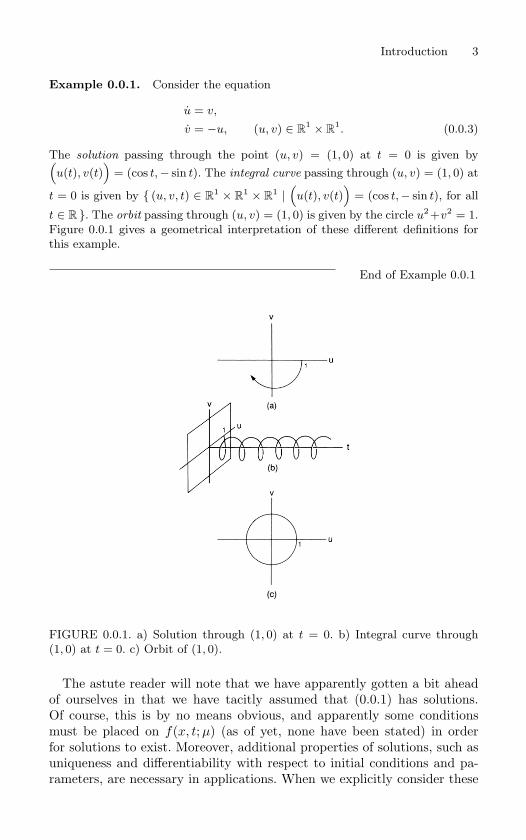
Example 0.0.1. Consider the equation
u = v,
v = −u, (u, v) ∈ R1 × R
1. (0.0.3)
The solution passing through the point (u, v) = (1, 0) at t = 0 is given by(u(t), v(t)
)= (cos t, − sin t). The integral curve passing through (u, v) = (1, 0) at
t = 0 is given by (u, v, t) ∈ R1 × R1 × R1 |(u(t), v(t)
)= (cos t, − sin t), for all
t ∈ R . The orbit passing through (u, v) = (1, 0) is given by the circle u2+v2 = 1.
Figure 0.0.1 gives a geometrical interpretation of these different definitions for
this example.
End of Example 0.0.1
FIGURE 0.0.1. a) Solution through (1, 0) at t = 0. b) Integral curve through
(1, 0) at t = 0. c) Orbit of (1, 0).
The astute reader will note that we have apparently gotten a bit aheadof ourselves in that we have tacitly assumed that (0.0.1) has solutions.Of course, this is by no means obvious, and apparently some conditionsmust be placed on f(x, t;µ) (as of yet, none have been stated) in orderfor solutions to exist. Moreover, additional properties of solutions, such asuniqueness and differentiability with respect to initial conditions and pa-rameters, are necessary in applications. When we explicitly consider these
4 Introduction
questions in Chapter 7, we will see that these properties also are inheritedfrom conditions on f(x, t;µ). For now, we will merely state without proofthat if f(x, t;µ) is Cr (r ≥ 1) in x, t, and µ then solutions through anyx0 ∈ R
n exist and are unique on some time interval. Moreover, the solu-tions themselves are Cr functions of t, t0, x0, and µ. (Note: recall that afunction is said to be Cr if it is r times differentiable and each derivativeis continuous; if r = 0 then the function is merely continuous.)
At this stage we have said nothing about maps, i.e., Equation (0.0.2).In a broad sense, we will study two types of maps depending on g(x; µ);noninvertible maps if g(x; µ) as a function of x for fixed µ has no inverse,and invertible maps if g(x;µ) has an inverse. The map will be referred toas a Cr diffeomorphism if g(x; µ) is invertible, with the inverse denotedg−1(x;µ), and both g(x;µ) and g−1(x; µ) are Cr maps (recall that a mapis invertible if it is one-to-one and onto). Our goal will be to study theorbits of (0.0.2), i.e., the bi-infinite (if g is invertible) sequences of points
· · · , g−n(x0;µ), · · · , g−1(x0;µ), x0, g(x0;µ), · · · gn(x0;µ), · · ·, (0.0.4)
where x0 ∈ U and gn is defined inductively by
gn(x0; µ) ≡ g(gn−1(x0;µ)
), n ≥ 2, (0.0.5)
g−n(x0; µ) ≡ g−1(g−n+1(x0;µ)), n ≥ 2, (0.0.6)
or the infinite (if g is noninvertible) sequences of points
x0, g(x0;µ), · · · , gn(x0; µ), · · ·, (0.0.7)
where x0 ∈ U and gn is defined inductively by (0.0.5). (Note: it shouldbe clear that we must assume gn−1(x0;µ), g−n+1(x0;µ) ∈ U , n ≥ 2, for(0.0.4) to make sense and gn−1(x0;µ) ∈ U , n ≥ 2, for (0.0.7) to make sense.)Notice that questions of existence and uniqueness of orbits for maps areobvious and that differentiability of orbits with respect to initial conditionsand parameters is a consequence of the applicability of the chain rule ofelementary calculus.
With these preliminaries out of the way, we can now turn to the mainbusiness of this book.
1
Equilibrium Solutions,Stability, and LinearizedStability
1.1 Equilibria of Vector Fields
Consider a general autonomous vector field
x = f(x), x ∈ Rn. (1.1.1)
An equilibrium solution of (1.1.1) is a point x ∈ Rn such that
f(x) = 0,
i.e., a solution which does not change in time. Other terms often substitutedfor the term “equilibrium solution” are “fixed point,” “stationary point,”“rest point,” “singularity,” “critical point,” or “steady state.” In this bookwe will utilize the terms equilibrium point or fixed point exclusively.
Example 1.1.1 (“Equilibria” in Nonautonomous Vector Fields). What about
the notion of equilibria for nonautonomous vector fields? This is a situation where
doing what “seems right” (i.e.. using ideas that have only been developed for
autonomous vector fields) can lead to incorrect results. Let is describe this in
more detail
Consider a nonautonomous vector field
x = f(x, t), x ∈ Rn.
A common way of viewing this in applications is to view time as ”frozen” and
look at equilibria of the frozen time vector field (this is often done in fluid me-
chanics where the vector field has the interpretation as the velocity field). These
“instantaneous” fixed points are given by
f(x, t) = 0.
If we can find a point (x, t) such that f(x, t) = 0 and Dxf(x, t) = 0, then by
the implicit function theorem we can find a function x(t), with x(t) = x such
that f(x(t), t) = 0, for t in some interval about t. However, these “frozen time
equilibria” are not solutions of the nonautonomous vector field. In fact, it is easy
6 1. Equilibrium Solutions, Stability, and Linearized Stability
to see that if x(t) is a solution of the nonautonomous vector field, then it must
be constant in time, i.e., ˙x(t) = 0, see Exercise 11.
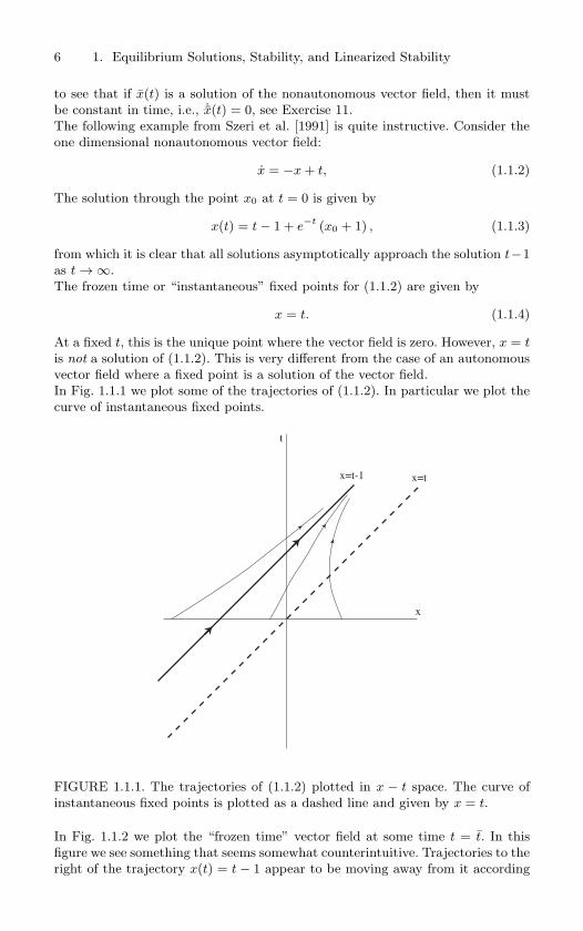
The following example from Szeri et al. [1991] is quite instructive. Consider the
one dimensional nonautonomous vector field:
x = −x + t, (1.1.2)
The solution through the point x0 at t = 0 is given by
x(t) = t − 1 + e−t(x0 + 1) , (1.1.3)
from which it is clear that all solutions asymptotically approach the solution t−1
as t → ∞.
The frozen time or “instantaneous” fixed points for (1.1.2) are given by
x = t. (1.1.4)
At a fixed t, this is the unique point where the vector field is zero. However, x = tis not a solution of (1.1.2). This is very different from the case of an autonomous
vector field where a fixed point is a solution of the vector field.
In Fig. 1.1.1 we plot some of the trajectories of (1.1.2). In particular we plot the
curve of instantaneous fixed points.
x
t
x=tx=t-1
FIGURE 1.1.1. The trajectories of (1.1.2) plotted in x − t space. The curve of
instantaneous fixed points is plotted as a dashed line and given by x = t.
In Fig. 1.1.2 we plot the “frozen time” vector field at some time t = t. In this
figure we see something that seems somewhat counterintuitive. Trajectories to the
right of the trajectory x(t) = t − 1 appear to be moving away from it according
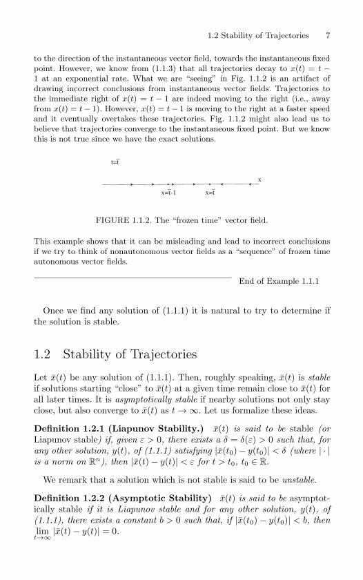
1.2 Stability of Trajectories 7
to the direction of the instantaneous vector field, towards the instantaneous fixed
point. However, we know from (1.1.3) that all trajectories decay to x(t) = t −1 at an exponential rate. What we are “seeing” in Fig. 1.1.2 is an artifact of
drawing incorrect conclusions from instantaneous vector fields. Trajectories to
the immediate right of x(t) = t − 1 are indeed moving to the right (i.e., away
from x(t) = t − 1). However, x(t) = t − 1 is moving to the right at a faster speed
and it eventually overtakes these trajectories. Fig. 1.1.2 might also lead us to
believe that trajectories converge to the instantaneous fixed point. But we know
this is not true since we have the exact solutions.
x
t=t_
x=t-1_
x=t_
FIGURE 1.1.2. The “frozen time” vector field.
This example shows that it can be misleading and lead to incorrect conclusions
if we try to think of nonautonomous vector fields as a “sequence” of frozen time
autonomous vector fields.
End of Example 1.1.1
Once we find any solution of (1.1.1) it is natural to try to determine ifthe solution is stable.
1.2 Stability of Trajectories
Let x(t) be any solution of (1.1.1). Then, roughly speaking, x(t) is stable
if solutions starting “close” to x(t) at a given time remain close to x(t) forall later times. It is asymptotically stable if nearby solutions not only stayclose, but also converge to x(t) as t →∞. Let us formalize these ideas.
Definition 1.2.1 (Liapunov Stability.) x(t) is said to be stable (or
Liapunov stable) if, given ε > 0, there exists a δ = δ(ε) > 0 such that, for
any other solution, y(t), of (1.1.1) satisfying |x(t0)− y(t0)| < δ (where | · |is a norm on R
n), then |x(t)− y(t)| < ε for t > t0, t0 ∈ R.
We remark that a solution which is not stable is said to be unstable.
Definition 1.2.2 (Asymptotic Stability) x(t) is said to be asymptot-ically stable if it is Liapunov stable and for any other solution, y(t), of
(1.1.1), there exists a constant b > 0 such that, if |x(t0)− y(t0)| < b, then
limt→∞
|x(t)− y(t)| = 0.
8 1. Equilibrium Solutions, Stability, and Linearized Stability
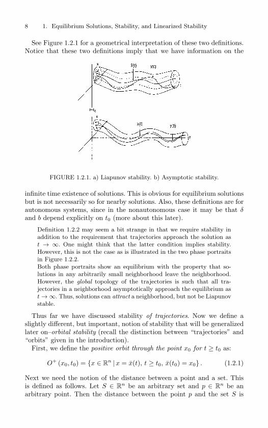
See Figure 1.2.1 for a geometrical interpretation of these two definitions.Notice that these two definitions imply that we have information on the
FIGURE 1.2.1. a) Liapunov stability. b) Asymptotic stability.
infinite time existence of solutions. This is obvious for equilibrium solutionsbut is not necessarily so for nearby solutions. Also, these definitions are forautonomous systems, since in the nonautonomous case it may be that δand b depend explicitly on t0 (more about this later).
Definition 1.2.2 may seem a bit strange in that we require stability in
addition to the requirement that trajectories approach the solution as
t → ∞. One might think that the latter condition implies stability.
However, this is not the case as is illustrated in the two phase portraits
in Figure 1.2.2.
Both phase portraits show an equilibrium with the property that so-
lutions in any arbitrarily small neighborhood leave the neighborhood.
However, the global topology of the trajectories is such that all tra-
jectories in a neighborhood asymptotically approach the equilibrium as
t → ∞. Thus, solutions can attract a neighborhood, but not be Liapunov
stable.
Thus far we have discussed stability of trajectories. Now we define aslightly different, but important, notion of stability that will be generalizedlater on–orbital stability (recall the distinction between “trajectories” and“orbits” given in the introduction).
First, we define the positive orbit through the point x0 for t ≥ t0 as:
O+ (x0, t0) = x ∈ Rn |x = x(t), t ≥ t0, x(t0) = x0 . (1.2.1)
Next we need the notion of the distance between a point and a set. Thisis defined as follows. Let S ∈ R
n be an arbitrary set and p ∈ Rn be an
arbitrary point. Then the distance between the point p and the set S is
1.2 Stability of Trajectories 9
(a)
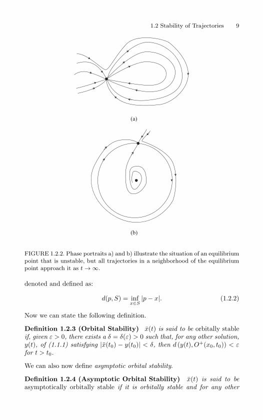
(b)
FIGURE 1.2.2. Phase portraits a) and b) illustrate the situation of an equilibrium
point that is unstable, but all trajectories in a neighborhood of the equilibrium
point approach it as t → ∞.
denoted and defined as:
d(p, S) = infx∈S
|p− x|. (1.2.2)
Now we can state the following definition.
Definition 1.2.3 (Orbital Stability) x(t) is said to be orbitally stableif, given ε > 0, there exists a δ = δ(ε) > 0 such that, for any other solution,
y(t), of (1.1.1) satisfying |x(t0) − y(t0)| < δ, then d (y(t), O+(x0, t0)) < εfor t > t0.
We can also now define asymptotic orbital stability.
Definition 1.2.4 (Asymptotic Orbital Stability) x(t) is said to be
asymptotically orbitally stable if it is orbitally stable and for any other
10 1. Equilibrium Solutions, Stability, and Linearized Stability
solution, y(t), of (1.1.1), there exists a constant b > 0 such that, if |x(t0)−y(t0)| < b, then lim
t→∞d(y(t), O+(x0, t0)
)= 0.
Definitions 1.2.3 and 1.2.4 are stated in terms of orbital stability of a tra-
jectory. In practice, variations in the terminology may arise. In particular,one could just as easily phrase these definitions in terms of the stability ofthe orbit (generated by the trajectory), rather than the trajectory. This isan example of where the distinction between “orbit” and “trajectory” isslightly blurred.
Definitions 1.2.1, 1.2.2, 1.2.3, 1.2.4 describe mathematically differenttypes of stability; however, they do not provide us with a method for deter-mining whether or not a given solution is stable. We now turn our attentionto this question.
1.2a LinearizationIn order to determine the stability of x(t) we must understand the natureof solutions near x(t). Let
x = x(t) + y. (1.2.3)
Substituting (1.2.3) into (1.1.1) and Taylor expanding about x(t) gives
x = ˙x(t) + y = f(x(t)
)+ Df
(x(t)
)y +O(|y|2), (1.2.4)
where Df is the derivative of f and | · | denotes a norm on Rn (note: in
order to obtain (1.2.4) f must be at least twice differentiable). Using thefact that ˙x(t) = f
(x(t)
), (1.2.4) becomes
y = Df(x(t)
)y +O(|y|2). (1.2.5)
Equation (1.2.5) describes the evolution of orbits near x(t). For stabilityquestions we are concerned with the behavior of solutions arbitrarily closeto x(t), so it seems reasonable that this question could be answered bystudying the associated linear system
y = Df(x(t)
)y. (1.2.6)
Therefore, the question of stability of x(t) involves the following two steps:
1. Determine if the y = 0 solution of (1.2.6) is stable.
2. Show that stability (or instability) of the y = 0 solution of (1.2.6)implies stability (or instability) of x(t).
Step 1 may be equally as difficult as our original problem, since there areno general analytical methods for finding the solution of linear ordinarydifferential equations with time-dependent coefficients. However, if x(t) is
1.2 Stability of Trajectories 11
an equilibrium solution, i.e., x(t) = x, then Df(x(t)
)= Df(x) is a matrix
with constant entries, and the solution of (1.1.6) through the point y0 ∈ Rn
of t = 0 can immediately be written as
y(t) = eDf(x)ty0. (1.2.7)
Thus, y(t) is asymptotically stable if all eigenvalues of Df(x) have negativereal parts (cf. Exercise 7).
The answer to Step 2 can be obtained from the following theorem.
Theorem 1.2.5 Suppose all of the eigenvalues of Df(x) have negative
real parts. Then the equilibrium solution x = x of the nonlinear vector field
(1.1.1) is asymptotically stable.
Proof: We will give the proof of this theorem in Chapter 2 when we discussLiapunov functions.
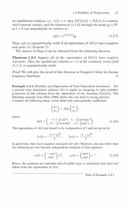
Example 1.2.1 (Stability and Eigenvalues of Time-Dependent Jacobians). For
a general time dependent solution x(t) it might be tempting to infer stability
properties of this solution from the eigenvalues of the Jacobian Df(x(t)). The
following example from Hale [1980] shows this can lead to wrong answers.
Consider the following linear vector field with time-periodic coefficients(x1
x2
)= A(t)
(x1
x2
),
where
A(t) =
( −1 + 32 cos2 t 1 − 3
2 cos t sin t−1 − 3
2 cos t sin t −1 + 32 sin2 t
). (1.2.8)
The eigenvalues of A(t) are found to be independent of t and are given by
λ1(t) =−1 + i
√7
4, λ2(t) =
−1 − i√
7
4.
In particular, they have negative real parts for all t. However, one can verify that
the following are two linearly independent solutions of this equation
v1(t) =
(− cos tsin t
)e
t2 , v2(t) =
(sin tcos t
)e−t. (1.2.9)
Hence, the solutions are unstable and of saddle type, a conclusion that does not
follow from the eigenvalues of A(t).
End of Example 1.2.1
12 1. Equilibrium Solutions, Stability, and Linearized Stability
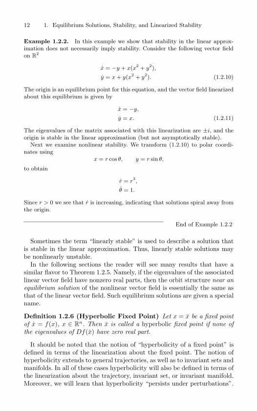
Example 1.2.2. In this example we show that stability in the linear approx-
imation does not necessarily imply stability. Consider the following vector field
on R2
x = −y + x(x2+ y2
),
y = x + y(x2+ y2
). (1.2.10)
The origin is an equilibrium point for this equation, and the vector field linearized
about this equilibrium is given by
x = −y,
y = x. (1.2.11)
The eigenvalues of the matrix associated with this linearization are ±i, and the
origin is stable in the linear approximation (but not asymptotically stable).
Next we examine nonlinear stability. We transform (1.2.10) to polar coordi-
nates using
x = r cos θ, y = r sin θ,
to obtain
r = r3,
θ = 1.
Since r > 0 we see that r is increasing, indicating that solutions spiral away from
the origin.
End of Example 1.2.2
Sometimes the term “linearly stable” is used to describe a solution thatis stable in the linear approximation. Thus, linearly stable solutions maybe nonlinearly unstable.
In the following sections the reader will see many results that have asimilar flavor to Theorem 1.2.5. Namely, if the eigenvalues of the associatedlinear vector field have nonzero real parts, then the orbit structure near an
equilibrium solution of the nonlinear vector field is essentially the same asthat of the linear vector field. Such equilibrium solutions are given a specialname.
Definition 1.2.6 (Hyperbolic Fixed Point) Let x = x be a fixed point
of x = f(x), x ∈ Rn. Then x is called a hyperbolic fixed point if none of
the eigenvalues of Df(x) have zero real part.
It should be noted that the notion of “hyperbolicity of a fixed point” isdefined in terms of the linearization about the fixed point. The notion ofhyperbolicity extends to general trajectories, as well as to invariant sets andmanifolds. In all of these cases hyperbolicity will also be defined in terms ofthe linearization about the trajectory, invariant set, or invariant manifold.Moreover, we will learn that hyperbolicity “persists under perturbations”.
1.2 Stability of Trajectories 13
Historically, hyperbolicity has been a central concept in the developmentof dynamical systems theory.
It should be clear that in our studies of stability of equilibria in the linear
approximation the nature of the linearized stability will boil down to a
study of the nature of the roots of the characteristic polynomial of the
matrix associated with the linearization about the equilibrium point of
interest. Here we collect together a few very useful results about the
roots of polynomials.
Consider a polynomial with real coefficients of the form:
p(λ) = a0λn
+ a1λn−1
+ · · · + an−1λ + an, ai ∈ R, a0 = 0. (1.2.12)
Theorem 1.2.7 (Fundamental Theorem of Algebra) (1.2.12) has exactlyn real or complex roots, λ1, . . . , λn, where repetition of roots is possible, i.e.,λi = λj, for some i and j.
Since we are considering the case of polynomials with real coefficients,it is easy to verify that if λ is a root of (1.2.12) then so is the complex
conjugate of λ, λ (just substitute the root λ into (1.2.12) and take the
complex conjugate of the result, using the fact that the coefficients are
real). Hence, for polynomials with real coefficients the roots occur in
complex conjugate pairs.
Next we describe a useful result that enables to get some information
about the roots of polynomials just by “looking at” the coefficients.
Theorem 1.2.8 (Descartes’ Rule of Signs) Consider the sequence of coefi-cients of (1.2.12):
an, an−1, · · · , a1, a0.
Let k be the total number of sign changes from one coefficient to the next in thesequence. Then the number of positive real roots of the polynomial is either equalto k, or k minus a positive even integer. (Note: if k = 1 then there is exactly onepositive real root.)
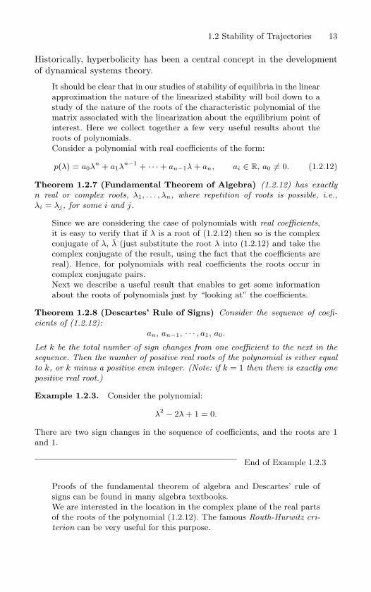
Example 1.2.3. Consider the polynomial:
λ2 − 2λ + 1 = 0.
There are two sign changes in the sequence of coefficients, and the roots are 1
and 1.
End of Example 1.2.3
Proofs of the fundamental theorem of algebra and Descartes’ rule of
signs can be found in many algebra textbooks.
We are interested in the location in the complex plane of the real parts
of the roots of the polynomial (1.2.12). The famous Routh-Hurwitz cri-terion can be very useful for this purpose.
14 1. Equilibrium Solutions, Stability, and Linearized Stability
First we construct the Routh table associated with the polynomial
(1.2.12). This is given by:
a0 a2 a4 a6 · · ·a1 a3 a5 a7 · · ·r3,1 r3,2 r3,3 r3,4 · · ·r4,1 r4,2 r4,3 r4,4 · · ·...
......
... · · ·rn+1,1 rn+1,2 rn+1,3 rn+1,4 · · ·
(1.2.13)
where
(ri,1 ri,2 · · ·) ≡ (ri−2,2 ri−2,3 · · ·) − ri−2,1
ri−1,1(ri−1,2 ri−1,3 · · ·) , (i > 2).
(1.2.14)
(The notation ri,j stands for row i, column j.) Note that rows three and
higher may not contain the same number of entries as rows one or two.
This will be seen in an example below. Now we state the following test.
Theorem 1.2.9 (Routh-Hurwitz Test) All of the roots of the polynomial(1.2.12) have real parts strictly less than zero if and only if all n + 1 elements inthe first column of the Routh table are nonzero and have the same sign.
An elementary proof of the Routh-Hurwitz criterion can be found in
Meinsma [1995]. A comprehensive reference is Gantmacher [1989], which
also covers certain “singular” cases not covered by the result stated here
(the so-called “regular case”).
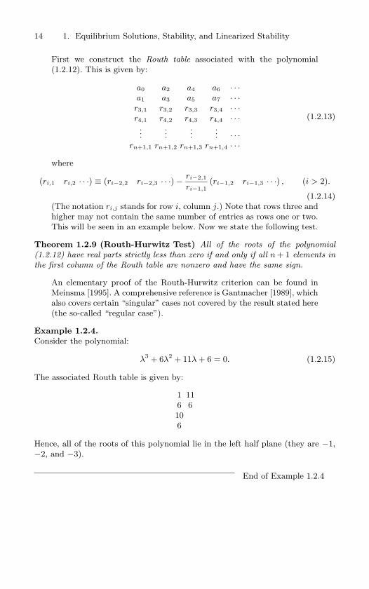
Example 1.2.4.Consider the polynomial:
λ3+ 6λ2
+ 11λ + 6 = 0. (1.2.15)
The associated Routh table is given by:
1 11
6 6
10
6
Hence, all of the roots of this polynomial lie in the left half plane (they are −1,
−2, and −3).
End of Example 1.2.4
1.3 Maps 15
1.3 Maps
Everything discussed thus far applies also for maps; we mention some ofthe details explicitly.
Consider a Cr (r ≥ 1) map
x → g(x), x ∈ Rn, (1.3.1)
and suppose that it has a fixed point at x = x, i.e., x = g(x). The associatedlinear map is given by
y → Ay, y ∈ Rn, (1.3.2)
where A ≡ Dg(x).
1.3a Definitions of Stability for MapsThe definitions of stability and asymptotic stability for orbits of maps arevery similar to the definitions for vector fields. We leave it as an exercisefor the reader to formulate these definitions (cf. Exercise 4).
1.3b Stability of Fixed Points of Linear MapsChoose a point y0 ∈ R
n. The orbit of y0 under the linear map (1.3.2) isgiven by the bi-infinite sequence (if the map is a Cr, r ≥ 1, diffeomorphism)
· · · , A−ny0, · · · , A−1y0, y0, Ay0, · · · , Any0, · · · (1.3.3)
or the infinite sequence (if the map is Cr, r ≥ 1, but noninvertible)
y0, Ay0, · · · , Any0, · · ·. (1.3.4)
From (1.3.3) and (1.3.4) it should be clear the fixed point y = 0 of thelinear map (1.3.2) is asymptotically stable if all of the eigenvalues of Ahave moduli strictly less than one (cf. Exercise 9).
1.3c Stability of Fixed Points of Maps via theLinear Approximation
With the obvious modifications, Theorem 1.2.5 is valid for maps.Before we apply these ideas to the unforced Duffing oscillator, let us first
give some useful terminology.
16 1. Equilibrium Solutions, Stability, and Linearized Stability
1.4 Some Terminology Associated with FixedPoints
A hyperbolic fixed point of a vector field (resp., map) is called a saddle ifsome, but not all, of the eigenvalues of the associated linearization have realparts greater than zero (resp., moduli greater than one) and the rest of theeigenvalues have real parts less than zero (resp., moduli less than one). Ifall of the eigenvalues have negative real part (resp., moduli less than one),then the hyperbolic fixed point is called a stable node or sink, and if all ofthe eigenvalues have positive real parts (resp., moduli greater than one),then the hyperbolic fixed point is called an unstable node or source. If theeigenvalues are purely imaginary (resp., have modulus one) and nonzero(resp., are not real), the nonhyperbolic fixed point is said to be a center
(resp., is said to be elliptic).Let us now apply our results to the unforced Duffing oscillator.
1.5 Application to the Unforced Duffing Oscillator
The unforced Duffing oscillator is given by
x = y,
y = x− x3 − δy, δ ≥ 0.
It is easy to see that this equation has three fixed points given by
(x, y) = (0, 0), (±1, 0). (1.5.1)
The matrix associated with the linearized vector field is given by(0 1
1− 3x2 −δ
). (1.5.2)
Using (1.5.1) and (1.5.2) the eigenvalues λ1 and λ2 associated with thefixed point (0, 0) are given by λ1,2 = −δ/2± 1
2
√δ2 + 4, and the eigenvalues
associated with the fixed points (±1, 0) are the same for each point and aregiven by λ1,2 = −δ/2 ± 1
2
√δ2 − 8. Hence, for δ > 0, (0, 0) is unstable and
(±1, 0) are asymptotically stable; for δ = 0, (±1, 0) are stable in the linearapproximation.
1.6 Exercises1. Consider the following vector fields.
a ) x = y,y = −δy − µx,
(x, y) ∈ R2.
1.6 Exercises 17
b)x = y,y = −δy − µx − x2,
(x, y) ∈ R2.
c)x = y,y = −δy − µx − x3,
(x, y) ∈ R2.
d)x = −δx − µy + xy,y = µx − δy + 1
2 (x2 − y2), (x, y) ∈ R2.
e) x = −x + x3,y = x + y,
(x, y) ∈ R2.
f)r = r(1 − r2),θ = cos 4θ,
(r, θ) ∈ R+ × S
1.
g)r = r(δ + µr2 − r4),θ = 1 − r2,
(r, θ) ∈ R+ × S
1.
h) θ = v,v = − sin θ − δv + µ,
(θ, v) ∈ S1 × R.
i) θ1 = ω1,
θ2 = ω2 + θn1 , n ≥ 1,
(θ1, θ2) ∈ S1 × S
1.
j) θ1 = θ2 − sin θ1,
θ2 = −θ2,(θ1, θ2) ∈ S
1 × S1.
k) θ1 = θ21 ,
θ2 = ω2,(θ1, θ2) ∈ S
1 × S1.
Find all fixed points and discuss their stability.
2. Consider the following maps.
a) x → x,y → x + y,
(x, y) ∈ R2.
b) x → x2,y → x + y,
(x, y) ∈ R2.
c) θ1 → θ1,θ2 → θ1 + θ2,
(θ1, θ2) ∈ S1 × S
1.
d) θ1 → sin θ1,θ2 → θ1,
(θ1, θ2) ∈ S1 × S
1.
e)x → 2xy
x+y ,
y →(
2xy2
x+y
)1/2,
(x, y) ∈ R2.
f) x → x+y2 ,
y → (xy)1/2,(x, y) ∈ R
2.
g) x → µ − δy − x2,y → x,
(x, y) ∈ R2.
h) θ → θ + v,v → δv − µ cos(θ + v), (θ, v) ∈ S
1 × R1.
Find all the fixed points and discuss their stability.
3. Consider a Cr (r ≥ 1) diffeomorphism
x → f(x), x ∈ Rn
.
Suppose f has a hyperbolic periodic orbit of period k. Denote the orbit by
O(p) =
p, f(p), f2(p), · · · , f
k−1(p), fk(p) = p
.
Show that stability of O(p) is determined by the linear map
y → Dfk(fj(p))y
for any j = 0, 1, · · · , k−1. Does the same result hold for periodic orbits of noninvertiblemaps?
18 1. Equilibrium Solutions, Stability, and Linearized Stability
4. Formulate the definitions of Liapunov stability and asymptotic stability for maps.
5. Show that hyperbolic fixed points of maps which are asymptotically stable in the linearapproximation are nonlinearly asymptotically stable.
6. Give examples of fixed points of vector fields and maps that are stable in the linearapproximation but are nonlinearly unstable.
7. Consider the linear vector field
x = Ax, x ∈ Rn
,
where A is an n × n constant matrix. Suppose all the eigenvalues of A have negativereal parts. Then prove that x = 0 is an asymptotically stable fixed point for this linearvector field. (Hint: utilize a linear transformation of the coordinates which transformsA into Jordan canonical form.)
8. Suppose that the matrix A in Exercise 7 has some eigenvalues with zero real parts(and the rest have negative real parts). Does it follow that x = 0 is stable? Answerthis question by considering the following example.
(x1x2
)=(
0 10 0
)(x1x2
).
9. Consider the linear mapx → Ax, x ∈ R
n,
where A is an n×n constant matrix. Suppose all of the eigenvalues of A have modulusless than one. Then prove that x = 0 is an asymptotically stable fixed point for thislinear map (use the same hint given for Exercise 7).
10. Suppose that the matrix A in Exercise 9 has some eigenvalues having modulus one(with the rest having modulus less than one). Does it follow that x = 0 is stable?Answer this question by considering the following example.
(x1x2
)→
(1 10 1
)(x1x2
).
11. Consider a nonautonomous vector field
x = f(x, t), x ∈ Rn
,
and suppose that x(t) is a function (defined for some interval of t) satisfying
f(x(t), t) = 0.
Prove that if x(t) is a trajectory of the vector field then it must be constant in time.
12. Consider the following vector field (Yang [2001]):
x = −x,
φ = 1,
θ = ω, (x, φ, θ) ∈ R × S1 × S
1,
where ω is an irrational number. Show that every trajectory is asymptotically orbitallystable.
13. Consider the following vector field (Yang [2001]):
θ = sin2θ + (1 − r)2,
r = r(1 − r), (θ, r) ∈ S1 × R.
Show that every trajectory, except r = 0, is asymptotically orbitally stable.
1.6 Exercises 19
14. Does Descartes’ rule of signs provide any information about the roots of the polynomialp(−λ), where p(λ) is given by (1.2.12)?
15. Use the Routh-Hurwitz test to determine the location of the roots of the followingpolynomials:
(a) λ3 − 3λ2 + 3λ − 1,
(b) λ3 + 3λ2 − 4,
(c) λ3 + λ2 + λ + 1.
2
Liapunov Functions
The method of Liapunov can often be used to determine the stability offixed points when the information obtained from linearization is incon-clusive (i.e., when the fixed point is nonhyperbolic). Liapunov theory is alarge area, and we will examine only an extremely small part of it; for moreinformation, see Lasalle and Lefschetz [1961]1.
The basic idea of the method is as follows (the method works in n-dimensions and also infinite dimensions, but for the moment we will de-scribe it pictorally in the plane). Suppose you have a vector field in theplane with a fixed point x, and you want to determine whether or not it isstable. Roughly speaking, according to our previous definitions of stabilityit would be sufficient to find a neighborhood U of x for which orbits startingin U remain in U for all positive times (for the moment we don’t distinguishbetween stability and asymptotic stability). This condition would be satis-fied if we could show that the vector field is either tangent to the boundaryof U or pointing inward toward x (see Figure 2.0.1). This situation shouldremain true even as we shrink U down onto x. Now, Liapunov’s methodgives us a way of making this precise; we will show this for vector fields inthe plane and then generalize our results to R
n.Suppose we have the vector field
x = f(x, y),y = g(x, y), (x, y) ∈ R
2, (2.0.1)
which has a fixed point at (x, y) (assume it is stable). We want to showthat in any neighborhood of (x, y) the above situation holds. Let V (x, y)be a scalar-valued function on R
2, i.e., V : R2 → R1 (and at least C1), with
1First, something should be said about the spelling of the name “Liapunov”,also spelled as “Lyapunov”, and , “Liapounoff”. The book of Lasalle and Lefschetz[1961] uses “Liapunov”. Hirsch and Smale [1974] use “Liapunov”, while Arnold[1973] uses “Lyapunov”. In the setting of “Lyapunov exponents” the “y” is moretypically used (although the influential paper of Eckmann and Ruelle [1985] uses“i”). A random check of the journal Systems & Control Letters over the past fewyears found both “Liapunov” and “Lyapunov” both used about the same numberof times. For this reason many references in the bibliography of this book willhave different spellings of “L · apunov”. From time to time we will also driftbetween different spellings when a particular spelling is more usually found inthe area under discussion.
2. Liapunov Functions 21
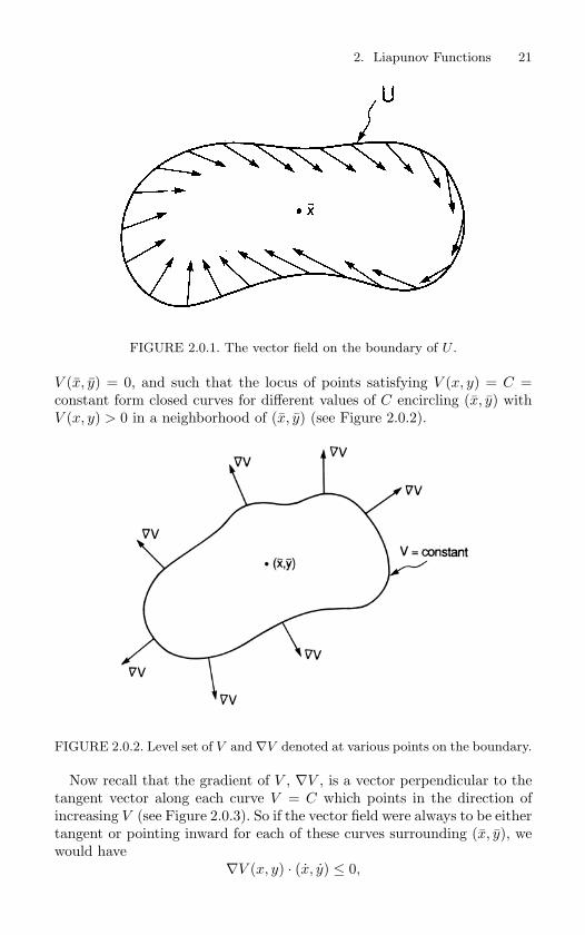
FIGURE 2.0.1. The vector field on the boundary of U .
V (x, y) = 0, and such that the locus of points satisfying V (x, y) = C =constant form closed curves for different values of C encircling (x, y) withV (x, y) > 0 in a neighborhood of (x, y) (see Figure 2.0.2).
FIGURE 2.0.2. Level set of V and ∇V denoted at various points on the boundary.
Now recall that the gradient of V , ∇V , is a vector perpendicular to thetangent vector along each curve V = C which points in the direction ofincreasing V (see Figure 2.0.3). So if the vector field were always to be eithertangent or pointing inward for each of these curves surrounding (x, y), wewould have
∇V (x, y) · (x, y) ≤ 0,
22 2. Liapunov Functions
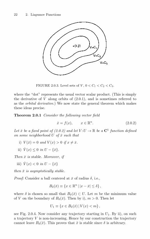
FIGURE 2.0.3. Level sets of V , 0 < C1 < C2 < C3.
where the “dot” represents the usual vector scalar product. (This is simplythe derivative of V along orbits of (2.0.1), and is sometimes referred toas the orbital derivative.) We now state the general theorem which makesthese ideas precise.
Theorem 2.0.1 Consider the following vector field
x = f(x), x ∈ Rn. (2.0.2)
Let x be a fixed point of (2.0.2) and let V : U → R be a C1 function defined
on some neighborhood U of x such that
i) V (x) = 0 and V (x) > 0 if x = x.
ii) V (x) ≤ 0 in U − x.
Then x is stable. Moreover, if
iii) V (x) < 0 in U − x
then x is asymptotically stable.
Proof: Consider a ball centered at x of radius δ, i.e.,
Bδ(x) ≡ x ∈ Rn | |x− x| ≤ δ ,
where δ is chosen so small that Bδ(x) ⊂ U . Let m be the minimum valueof V on the boundary of Bδ(x). Then by i), m > 0. Then let
U1 ≡ x ∈ Bδ(x) |V (x) < m ,
see Fig. 2.0.4. Now consider any trajectory starting in U1. By ii), on sucha trajectory V is non-increasing. Hence by our construction the trajectorycannot leave Bδ(x). This proves that x is stable since δ is arbitrary.
2. Liapunov Functions 23
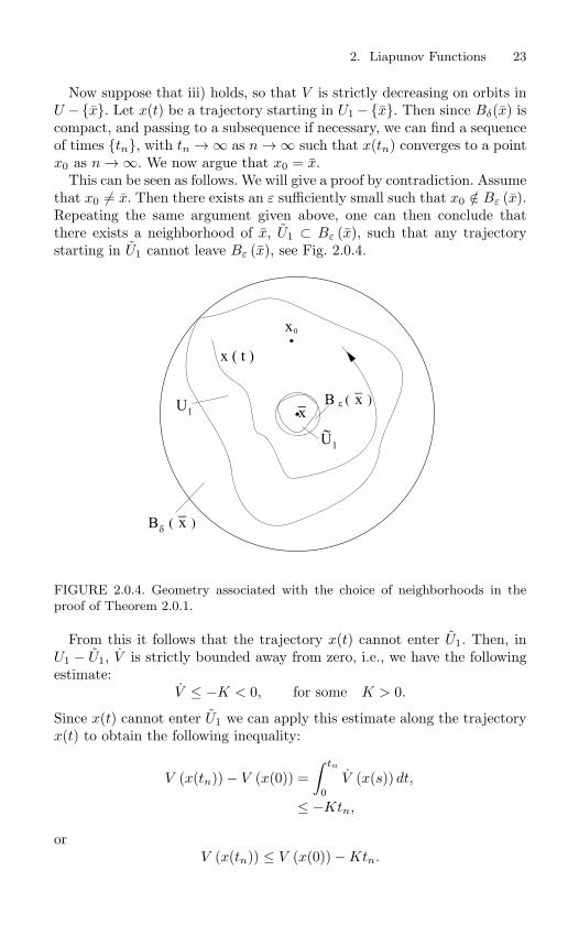
Now suppose that iii) holds, so that V is strictly decreasing on orbits inU −x. Let x(t) be a trajectory starting in U1−x. Then since Bδ(x) iscompact, and passing to a subsequence if necessary, we can find a sequenceof times tn, with tn →∞ as n →∞ such that x(tn) converges to a pointx0 as n →∞. We now argue that x0 = x.
This can be seen as follows. We will give a proof by contradiction. Assumethat x0 = x. Then there exists an ε sufficiently small such that x0 /∈ Bε (x).Repeating the same argument given above, one can then conclude thatthere exists a neighborhood of x, U1 ⊂ Bε (x), such that any trajectorystarting in U1 cannot leave Bε (x), see Fig. 2.0.4.
x_
x0
1U
B x_
x ( t )
B x_
1U
FIGURE 2.0.4. Geometry associated with the choice of neighborhoods in the
proof of Theorem 2.0.1.
From this it follows that the trajectory x(t) cannot enter U1. Then, inU1 − U1, V is strictly bounded away from zero, i.e., we have the followingestimate:
V ≤ −K < 0, for some K > 0.
Since x(t) cannot enter U1 we can apply this estimate along the trajectoryx(t) to obtain the following inequality:
V (x(tn))− V (x(0)) =∫ tn
0V (x(s)) dt,
≤ −Ktn,
orV (x(tn)) ≤ V (x(0))−Ktn.
24 2. Liapunov Functions
Now as n →∞ this inequality imples that V (x(tn)) must become negative.This is a contradiction, which came about by assuming x0 = x. Thereforex = x0.
We remark that there is a slight gap in the proof of this theorem in thatwe have not proved that the trajectory x(t) exists on the semi-infinite timeinterval t ∈ [0,∞). Indeed, we have not considered existence of solutionsat all at this point in the book. Nevertheless, this fact is indeed true underour assumptions, see Theorem 7.2.1.
We refer to V as a Liapunov function. If V < 0 on U − x the termstrict Liapunov function is often used. We remark that if U can be chosento be all of R
n, then x is said to be globally asymptotically stable, if i) andiii) hold.
Example 2.0.1. Consider the following vector field
x = y, (2.0.3)
y = −x + εx2y. (2.0.4)
It is easy to verify that (2.0.3) has a nonhyperbolic fixed point at (x, y) = (0, 0).
Our goal is to determine if this fixed point is stable.
Let V (x, y) = (x2 + y2)/2. Clearly V (0, 0) = 0 and V (x, y) > 0 in any neigh-
borhood of (0, 0). Then
V (x, y) = ∇V (x, y) · (x, y)
= (x, y) · (y, εx2y − x)
= xy + εx2y2 − xy
and hence V = εx2y2. Then, by Theorem 2.0.1, (0, 0) is globally stable for ε < 0.
Actually, with a little more work, one can show that (0, 0) is globally asymptot-
ically stable for ε < 0
End of Example 2.0.1
Let us now use Liapunov theory to give an outline of the proof of Theorem1.2.5. We begin by recalling the set-up of the problem.
Consider the vector field
x = f(x), x ∈ Rn, (2.0.5)
and suppose that (2.0.5) has a fixed point at x = x, i.e., f(x) = 0. Wetranslate the fixed point to the origin via the coordinate shift y = x− x sothat (1.1.17) becomes
y = f(y + x), y ∈ Rn. (2.0.6)
Taylor expanding (2.0.6) about x gives
y = Df(x)y + R(y), (2.0.7)
2.1 Exercises 25
where R(y) ≡ O(|y|2).Now let us introduce the coordinate rescaling
y = εu, 0 < ε < 1. (2.0.8)
Thus, taking ε small implies making y small. Under (2.0.8) equation (2.0.7)becomes
u = Df(x)u + R(u, ε), (2.0.9)
where R(u, ε) = R(εu)/ε. It should be clear that R(u, 0) = 0 since R(y) =O(|y|2). We choose as a Liapunov function
V (u) =12|u|2.
Therefore,
V (u) = ∇V (u) · u=
(u ·Df(x)u
)+
(u · R(u, ε)
). (2.0.10)
From linear algebra the reader should recall that if all eigenvalues of Df(x0)have negative real part, then there exists a basis such that(
u ·Df(x0)u)
< k|u|2 < 0 (2.0.11)
for some real number k and for all u (see Arnold [1973] or Hirsch andSmale [1974] for a proof). Hence, by choosing ε sufficiently small, (2.0.10) isstrictly negative, which implies that the fixed point x = x is asymptoticallystable. We leave it to the reader to show that this result does not dependon the particular basis for which (2.0.11) holds. This latter point, whilesounding simple in practice, is much more tricky than one might believe,see Arnold [1973] or Hirsch and Smale [1974] for details.
2.1 Exercises1. Suppose x = x(t) is a solution of the nonautonomous equation
x = f(x, t), x ∈ Rn
.
Show that this solution can be transformed to the “zero solution” by the shift
x = y + x(t).
Hence, conclude that without loss of generality, the study of the stability of an arbitrarysolution can be transformed to a study of the stability of the solution x = 0, even fortime-dependent vector fields.
2. In this exercise we generalize Liapunov’s theorem to nonautonomous systems. Considera Cr, r ≥ 1, vector field
x = f(x, t), x ∈ Rn
, (2.1.1)
satisfyingf(0, t) = 0.
26 2. Liapunov Functions
Definition 2.1.1 A function V (x, t) is called positive definite in a region U ⊂ Rn if there
exists a function W (x) with the following properties:
1. W is defined and continuous in U.
2. 0 < W (x) ≤ V (x, t) for x = 0 and t ≥ t0.
The derivative of V along trajectories of (2.1.1) is given by
V ≡ ∂V
∂t+ ∇V · x
=∂V
∂t+ ∇V · f(x, t).
This is the orbital derivative for nonautonomous systems. Prove the following theorem.
Theorem 2.1.2 Suppose V (x, t) is positive definite in a neighborhood U of x = 0 fort ≥ t0. Then
i) if V (x, t) ≤ 0 in U.
x = 0 is stable. Moreover, if
ii) V (x, t) < 0 in U
then x = 0 is asymptotically stable.
Hint: Since in the definition of positive definite W (x) is independent of t, you should beable to mimic the proof of Theorem 2.0.1. For more information on Liapunov’s method fornonautonomous systems see Aeyels [1995].
3. Prove Dirichlet’s theorem (Siegel and Moser [1971]). Consider a Cr vector field (r ≥ 1)
x = f(x), x ∈ Rn
,
which has a fixed point at x = x. Let H(x) be a first integral of this vector field definedin a neighborhood of x = x such that x = x is a nondegenerate minimum of H(x).Then x = x is stable.
4. Prove Liapunov’s theorem for maps, i.e., consider a Cr diffeomorphism
x → f(x), x ∈ Rn
,
and suppose that we have a scalar-valued function
V : U → R1
defined on some open set U ∈ Rn satisfying
i) V (x0) = 0;
ii) V (x) > 0 for x = x0;
iii) V f(x) ≤ V (x) with equality if and only if x = x0.
Then x = x0 is a stable fixed point. Moreover, if strict inequality holds in iii), then x = x0 isasymptotically stable. Does the same result hold for noninvertible maps?
5. Consider the vector field
x = −y − x(x2 + y2),
y = x − y(x2 + y2), (x, y) ∈ R
2.
Use Liapunov’s method to show that the origin is globally asymptotically stable.
2.1 Exercises 27
6. Consider the damped Duffing equation
x = y,
y = x − x3 − δy, (x, y) ∈ R
2, δ > 0.
Use the function
V (x, y) =y2
2− x2
2+
x4
4,
as a Liapunov function to show that the equilibrium points (x, y) = (±1, 0) are asymp-totically stable.
7. Consider a particle of mass m moving in R3 under the influence of a potential field
Φ(x, y, z). The equations of motion are given by
mx = − ∂Φ∂x
(x, y, z),
my = − ∂Φ∂y
(x, y, z),
mz = − ∂Φ∂z
(x, y, z),
Prove that a minimum of the potential corresponds to a stable equilbrium point. Is itasymptotically stable? How differentiable must Φ(x, y, z) be?
8. Prove the following instability theorem. Let x = x be an equilibrium point of a Cr,r ≥ 1, vector field x = f(x), x ∈ R
n. Suppose V (x) is a C1 scalar valued functionsatisfying V (x) = 0 and V > 0 in U − x, where U is a neighborhood of x. IfV (xn) > 0 for some sequence xn → x, then x is unstable.
3
Invariant Manifolds: Linear andNonlinear Systems
We will see throughout this book that invariant manifolds, in particularstable, unstable, and center manifolds, play a central role in the analysis ofdynamical systems. We will give a simultaneous discussion of these ideasfor both vector fields
x = f(x), x ∈ Rn, (3.0.1)
and mapsx → g(x), x ∈ R
n. (3.0.2)
Definition 3.0.3 (Invariant Set) Let S ⊂ Rn be a set, then
a) (Continuous time) S is said to be invariant under the vector field
x = f(x) if for any x0 ∈ S we have x(t, 0, x0) ∈ S for all t ∈ R
(where x(0, 0, x0) = x0).
b) (Discrete time) S is said to be invariant under the map x → g(x) if
for any x0 ∈ S we have gn(x0) ∈ S for all n.
If we restrict ourselves to positive times (i.e., t ≥ 0, n ≥ 0) then we refer
to S as a positively invariant set and, for negative time, as a negativelyinvariant set.
Stated succinctly, invariant sets have the property that trajectories start-ing in the invariant set, remain in the invariant set, for all of their future,and all of their past.
We remark that if g is noninvertible, then only n ≥ 0 makes sense (al-though in some instances it may be useful to consider g−1 which does havea set theoretic meaning).
Definition 3.0.4 (Invariant Manifold) An invariant set S ⊂ Rn is said
to be a Cr (r ≥ 1) invariant manifold if S has the structure of a Cr
differentiable manifold. Similarly, a positively (resp., negatively) invariant
set S ⊂ Rn is said to be a Cr (r ≥ 1) positively (resp., negatively) invariant
manifold if S has the structure of a Cr differentiable manifold.
Evidently, we need to say what we mean by the term “Cr differentiablemanifold.” However, this is the subject of a course in itself, so rather than
3.1 Stable, Unstable, and Center Subspaces 29
define the concept of a manifold in its full generality, we will describe onlythat portion of the vast theory that we will need.
Roughly speaking, a manifold is a set which locally has the structureof Euclidean space. In applications, manifolds are most often met as m-dimensional surfaces embedded in R
n. If the surface has no singular points,i.e., the derivative of the function representing the surface has maximalrank, then by the implicit function theorem it can locally be representedas a graph. The surface is a Cr manifold if the (local) graphs representingit are Cr (note: for a thorough treatment of this particular representationof a manifold see Dubrovin, Fomenko, and Novikov [1985]).
Another example is even more basic. Let s1, · · · , sn denote the stan-dard basis on R
n. Let si1 , · · · , sij, j < n, denote any j basis vectors fromthis set; then the span of si1 , · · · , sij
forms a j-dimensional subspace ofR
n which is trivially a C∞ j-dimensional manifold. For a thorough intro-duction to the theory of manifolds with a view to applications see Abraham,Marsden, and Ratiu [1988].
The main reason for choosing these examples is that, in this book, whenthe term “manifold” is used, it will be sufficient to think of one of thefollowing two situations:
1. Linear Settings: a linear vector subspace of Rn;
2. Nonlinear Settings: a surface embedded in Rn which can be locally
represented as a graph (which can be justified via the implicit functiontheorem).
3.1 Stable, Unstable, and Center Subspaces ofLinear, Autonomous Vector Fields
Let us return to our study of the orbit structure near fixed points to seehow some important invariant manifolds arise. We begin with vector fields.Let x ∈ R
n be a fixed point of
x = f(x), x ∈ Rn. (3.1.1)
Then, by the discussion in Chapter 1, it is natural to consider the associatedlinear system
y = Ay, y ∈ Rn, (3.1.2)
where A ≡ Df(x) is a constant n×n matrix. The solution of (3.1.2) throughthe point y0 ∈ R
n at t = 0 is given by
y(t) = eAty0, (3.1.3)
whereeAt = id +At +
12!
A2t2 +13!
A3t3 + · · · (3.1.4)
30 3. Invariant Manifolds: Linear and Nonlinear Systems
and “id” denotes the n × n identity matrix. We must assume sufficientbackground in the theory of linear constant coefficient ordinary differentialequations so that (3.1.3) and (3.1.4) make sense to the reader. Excellentreferences for this theory are Arnold [1973] and Hirsch and Smale [1974].Our goal here is to extract the necessary ingredients from this theory so asto give a geometrical interpretation to (3.1.3).
Now Rn can be represented as the direct sum of three subspaces denoted
Es, Eu, and Ec, which are defined as follows:
Es = spane1, · · · , es,Eu = spanes+1, · · · , es+u, s + u + c = n, (3.1.5)Ec = spanes+u+1, · · · , es+u+c,
where e1, · · · , es are the (generalized) eigenvectors of A correspondingto the eigenvalues of A having negative real part, es+1, · · · , es+u are the(generalized) eigenvectors of A corresponding to eigenvalues of A havingpositive real part, and es+u+1, · · · , es+u+c are the (generalized) eigenvec-tors of A corresponding to the eigenvalues of A having zero real part (note:this is proved in great detail in Hirsch and Smale [1974]). Es, Eu, andEc are referred to as the stable, unstable, and center subspaces, respec-tively. They are also examples of invariant subspaces (or manifolds) sincesolutions of (3.1.2) with initial conditions entirely contained in either Es,Eu, or Ec must forever remain in that particular subspace for all time (wewill motivate this a bit more shortly). Moreover, solutions starting in Es
approach y = 0 asymptotically as t → +∞ and solutions starting in Eu
approach y = 0 asymptotically as t → −∞.We will now describe the linear algebra behind the definition of the
stable, unstable, and center subspaces in more detail, largely following thediscussion in Hirsch and Smale [1974], to which we refer the reader forproofs of some of the statements. We denote the eigenvalues of the (real)matrix A by
λs,1, · · · , λs,i, µs,1, µs,1, · · · , µs,j , µs,j i + 2j = s,
λu,1, · · · , λu,k, µu,1, µu,1, · · · , µu,l, µu,l k + 2l = u,
λc,1, · · · , λc,m, µc,1, µc,1, · · · , µc,n, µc,n m + 2n = c,
where λα,γ denote the real eigenvalues and µα,γ denotes complex eigenval-ues. Since A is real, if µα,γ is an eigenvalue of A so is µα,γ .
The generalized eigenspace corresponding to the (real) eigenvalue λα,γ isdefined as
V (A, λα,γ) ≡ Ker (A− λα,γ id)nα,γ , α = s, u, c, γ = i, k, m,
where nα,γ is the (algebraic) multiplicity of the eigenvalue λα,γ (i.e., thenumber of times it appears as a root of the characteristic polynomial as-
3.1 Stable, Unstable, and Center Subspaces 31
sociated with A, det (A− λ id) = 0). The dimension of V (A, λα,γ) is equalto nα,γ .
There is a bit of clumsiness with the notation here with respect to theeigenvalues with zero real part. The only way an eigenvalues can have zeroreal part, and be on the imaginary axis, is for it to be identically zero.Therefore λc,i = 0, i = 1, . . . , m, and it follows that nc,i = m, i = 1, . . . , m.
Complex eigenvalues are a bit more difficult to treat (actually, the dif-ficulty arises in the explanation; their treatment is fairly straightforward).Of course, the problem facing us is fairly evident. For a given complexeigenvalue µα,γ we can define the corresponding generalized eigenspace inthe usual way, i.e.,
V (A, µα,γ) ≡ Ker (A− µα,γ id)nα,γ , α = s, u, c, γ = j, l, n,
where nα,γ is the (algebraic) multiplicity of the eigenvalue µα,γ . However,if one applies the same technique as one applies for real eigenvalues tocompute the corresponding generalized eigenvectors one obtains complex
generalized eigenvectors. Clearly, this is not a satisfactory situation sincethe phase space of our dynamical system is real. Nevertheless, one canderive a real basis for the generalized eigenspace corresponding to a complexeigenvalue from these “complex generalized eigenvectors” by adopting thecomplexification stratagem, which we now describe. First, we must giveseveral definitions.
Let us think of Rn as a subset of C
n in the natural way, i.e., Rn is the
set of complex n-tuples where each entry is a real number.
Definition 3.1.1 Let F be a complex subspace of Cn. Then FR ≡ F ∩ R
n
is the set of n-tuples in F that are real. FR is referred to as the set of realvectors in F .
It can easily be shown that FR is closed under the operations of addition,as well as scalar multiplication by real numbers. Hence, FR is a real vectorspace (a subspace of R
n).
Definition 3.1.2 (Complexification of a Subspace) Let E be a sub-
space of Rn. Then
EC ≡
z ∈ Cn | z =
∑αixi, xi ∈ E, αi ∈ C
,
is called the complexification of E, where the sum denotes arbitrary, but
finite, linear combinations.
It is not hard to show that EC is a complex subspace of Cn, and that
(EC)R
= E.
Definition 3.1.3 (Complexification of a Real Linear Map) Suppose
A : Rn → R
n is a real linear map, and let E be a real subspace of Rn that
32 3. Invariant Manifolds: Linear and Nonlinear Systems
is invariant under A. The complexification of A, denoted AC, is a linear
map of EC into EC, and is defined as follows. By the definition of EC, any
z ∈ EC can be represented as
z =∑
αixi, xi ∈ E, αi ∈ C,
where the sum denotes arbitrary, but finite, linear combinations. Then we
define
ACz ≡∑
αiAxi.
Finally, we are at the point where we can define the generalizedeigenspace corresponding to a complex eigenvalue µα,γ . This is given by
V (A, µα,γ , µα,γ) ≡ (V (AC, µα,γ)⊕ V (AC, µα,γ)) ∩ Rn,
α = s, u, c, γ = j, l, n,
whereV (AC, µα,γ) ≡ Ker (AC − µα,γ id)nα,γ .
We then define the stable, unstable, and center subspaces as follows
Es ≡i∑
γ=1
V (A, λs,γ) +j∑
γ=1
V (A, µs,γ , µs,γ) , (3.1.6)
Eu ≡k∑
γ=1
V (A, λu,γ) +l∑
γ=1
V (A, µu,γ , µu,γ) , (3.1.7)
Ec ≡ V (A, 0) +n∑
γ=1
V (A, µc,γ , µc,γ) , (3.1.8)
where the sums are taken to be direct sums. By the primary decompositiontheorem (Hirsch and Smale [1974]) we have
Rn = Es ⊕ Eu ⊕ Ec.
3.1a Invariance of the Stable, Unstable, andCenter Subspaces
Let us outline how one ascertains the invariance of these subspaces underthe linear flow given in (3.1.3) (this will provide some useful hints for theexercises). First, consider the matrix A associated with the linear vectorfield (3.1.2) as a linear map of R
n into Rn. Clearly, Es, Eu, and Ec are
invariant subspaces for this linear map since each is the subspace spannedby a particular collection of generalized eigenvectors. We want to argue thatthey are invariant under the linear map eAt. This relies on the followingthree facts that are proven in a basic linear algebra course.
Suppose V ⊂ Rn is a subspace and invariant under the linear map A.
Then
3.1 Stable, Unstable, and Center Subspaces 33
• For any c ∈ R, V is invariant with respect to cA.
• For any integer n > 1, V is invariant with respect to An.
• Suppose A1 and A2 are linear maps on Rn and V is invariant with
respect to both A1 and A2. Then V is invariant with respect to A1 +A2. From this result it also follows that for any finite number oflinear maps Ai, i = 1, . . . , n, with V invariant under each, V is alsoinvariant under
∑ni=1 Ai.
Using each of these facts one can easily conclude that V is invariantunder the linear map
Ln(t) ≡ id + At +12A2t2 + · · ·+ 1
n!Antn =
n∑i=0
1i!
Aiti,
for any n, where id is the n × n identity matrix (and 0! ≡ 1). Now usingthe fact that V is closed, and that Ln(t) converges to eAt uniformly, weconclude that V is invariant with respect to eAt.
3.1b Some ExamplesWe now illustrate these ideas with three examples where for simplicity andeasier visualization we will work in R
3.
Example 3.1.1. Suppose the three eigenvalues of A are real and distinct and
denoted by λ1, λ2 < 0, λ3 > 0. Then A has three linearly independent eigenvec-
tors e1, e2, and e3 corresponding to λ1, λ2, and λ3, respectively. If we form the
3 × 3 matrix T by taking as columns the eigenvectors e1, e2, and e3, which we
write as
T ≡
...
......
e1 e2 e3...
......
, (3.1.9)
then we have
Λ ≡λ1 0 0
0 λ2 0
0 0 λ3
= T −1AT. (3.1.10)
Recall that the solution of (3.1.2) through y0 ∈ R3 at t = 0 is given by
y(t) = eAty0 = eTΛT −1ty0. (3.1.11)
Using (3.1.4), it is easy to see that (3.1.11) is the same as
y(t) = TeΛtT −1y0
= T
eλ1t 0 0
0 eλ2t 0
0 0 eλ3t
T −1y0
34 3. Invariant Manifolds: Linear and Nonlinear Systems
=
...
......
e1eλ1t e2e
λ2t e3eλ3t
......
...
T −1y0. (3.1.12)
Now we want to give a geometric interpretation to (3.1.12). Recall from (3.1.5)
that we have
Es= spane1, e2,
Eu= spane3.
Invariance
Choose any point y0 ∈ R3. Then T −1 is the transformation matrix which changes
the coordinates of y0 with respect to the standard basis on R3 (i.e., (1, 0, 0),
(0, 1, 0), (0, 0, 1)) into coordinates with respect to the basis e1, e2, and e3. Thus,
for y0 ∈ Es, T −1y0 has the form
T −1y0 =
y01
y02
0
, (3.1.13)
and, for y0 ∈ Eu, T −1y0 has the form
T −1y0 =
0
0
y03
. (3.1.14)
Therefore, by substituting (3.1.13) (resp., (3.1.14)) into (3.1.12), it is easy to see
that y0 ∈ Es (resp., Eu) implies eAty0 ∈ Es (resp., Eu). Thus, Es and Eu are
invariant manifolds.
Asymptotic Behavior
Using (3.1.13) and (3.1.12), we can see that, for any y0 ∈ Es, we have eAty0 → 0
as t → +∞ and, for any y0 ∈ Eu, we have eAty0 → 0 as t → −∞ (hence the
reason behind the names stable and unstable manifolds).
See Figure 3.1.1 for an illustration of the geometry of Es and Eu.
End of Example 3.1.1
Example 3.1.2. Suppose A has two complex conjugate eigenvalues ρ ± i ω,
ρ < 0, ω = 0 and one real eigenvalue λ > 0. Then A has three real generalized
eigenvectors e1, e2, and e3, which can be used as the columns of a matrix T in
order to transform A as follows
Λ ≡ ρ ω 0
−ω ρ 0
0 0 λ
= T −1AT. (3.1.15)
From Example 3.1.1 it is easy to see that in this example we have
y(t) = TeΛtT −1y0
= T
eρt cos ωt eρt sin ωt 0
−eρt sin ωt eρt cos ωt 0
0 0 eλt
T −1y0. (3.1.16)
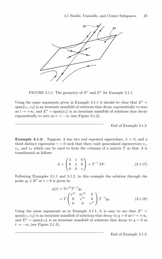
3.1 Stable, Unstable, and Center Subspaces 35
FIGURE 3.1.1. The geometry of Es and Eu for Example 3.1.1.
Using the same arguments given in Example 3.1.1 it should be clear that Es =
spane1, e2 is an invariant manifold of solutions that decay exponentially to zero
as t → +∞, and Eu = spane3 is an invariant manifold of solutions that decay
exponentially to zero as t → −∞ (see Figure 3.1.2).
End of Example 3.1.2
Example 3.1.3. Suppose A has two real repeated eigenvalues, λ < 0, and a
third distinct eigenvalue γ > 0 such that there exist generalized eigenvectors e1,
e2, and e3 which can be used to form the columns of a matrix T so that A is
transformed as follows
Λ =
λ 1 0
0 λ 0
0 0 γ
= T −1AT. (3.1.17)
Following Examples 3.1.1 and 3.1.2, in this example the solution through the
point y0 ∈ R3 at t = 0 is given by
y(t) = TeΛtT −1y0
= T
eλt teλt 0
0 eλt 0
0 0 eγt
T −1y0. (3.1.18)
Using the same arguments as in Example 3.1.1, it is easy to see that Es =
spane1, e2 is an invariant manifold of solutions that decay to y = 0 as t → +∞,
and Eu = spane3 is an invariant manifold of solutions that decay to y = 0 as
t → −∞ (see Figure 3.1.3).
End of Example 3.1.3
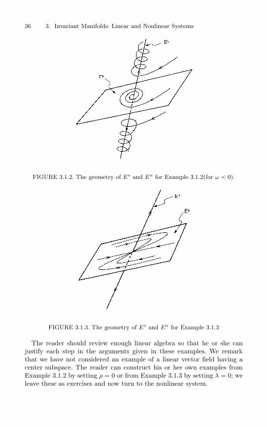
36 3. Invariant Manifolds: Linear and Nonlinear Systems
FIGURE 3.1.2. The geometry of Es and Eu for Example 3.1.2(for ω < 0).
FIGURE 3.1.3. The geometry of Es and Eu for Example 3.1.3
The reader should review enough linear algebra so that he or she canjustify each step in the arguments given in these examples. We remarkthat we have not considered an example of a linear vector field having acenter subspace. The reader can construct his or her own examples fromExample 3.1.2 by setting ρ = 0 or from Example 3.1.3 by setting λ = 0; weleave these as exercises and now turn to the nonlinear system.
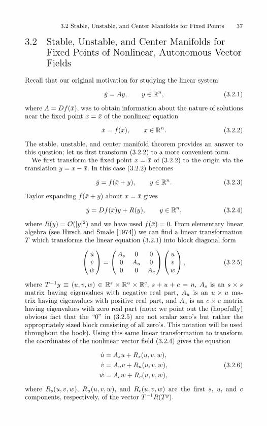
3.2 Stable, Unstable, and Center Manifolds for Fixed Points 37
3.2 Stable, Unstable, and Center Manifolds forFixed Points of Nonlinear, Autonomous VectorFields
Recall that our original motivation for studying the linear system
y = Ay, y ∈ Rn, (3.2.1)
where A = Df(x), was to obtain information about the nature of solutionsnear the fixed point x = x of the nonlinear equation
x = f(x), x ∈ Rn. (3.2.2)
The stable, unstable, and center manifold theorem provides an answer tothis question; let us first transform (3.2.2) to a more convenient form.
We first transform the fixed point x = x of (3.2.2) to the origin via thetranslation y = x− x. In this case (3.2.2) becomes
y = f(x + y), y ∈ Rn. (3.2.3)
Taylor expanding f(x + y) about x = x gives
y = Df(x)y + R(y), y ∈ Rn, (3.2.4)
where R(y) = O(|y|2) and we have used f(x) = 0. From elementary linearalgebra (see Hirsch and Smale [1974]) we can find a linear transformationT which transforms the linear equation (3.2.1) into block diagonal form
uvw
=
As 0 0
0 Au 00 0 Ac
u
vw
, (3.2.5)
where T−1y ≡ (u, v, w) ∈ Rs × R
u × Rc, s + u + c = n, As is an s × s
matrix having eigenvalues with negative real part, Au is an u × u ma-trix having eigenvalues with positive real part, and Ac is an c × c matrixhaving eigenvalues with zero real part (note: we point out the (hopefully)obvious fact that the “0” in (3.2.5) are not scalar zero’s but rather theappropriately sized block consisting of all zero’s. This notation will be usedthroughout the book). Using this same linear transformation to transformthe coordinates of the nonlinear vector field (3.2.4) gives the equation
u = Asu + Rs(u, v, w),v = Auv + Ru(u, v, w), (3.2.6)w = Acw + Rc(u, v, w),
where Rs(u, v, w), Ru(u, v, w), and Rc(u, v, w) are the first s, u, and ccomponents, respectively, of the vector T−1R(T y).
38 3. Invariant Manifolds: Linear and Nonlinear Systems
Now consider the linear vector field (3.2.5). From our previous discussion(3.2.5) has an s-dimensional invariant stable manifold, a u-dimensional in-variant unstable manifold, and a c-dimensional invariant center manifold allintersecting in the origin. The following theorem shows how this structurechanges when the nonlinear vector field (3.2.6) is considered.
Theorem 3.2.1 (Local Stable, Unstable, and Center Manifolds ofFixed Points) Suppose (3.2.6) is Cr, r ≥ 2. Then the fixed point
(u, v, w) = 0 of (3.2.6) possesses a Cr s-dimensional local, invariant stable
manifold, W sloc(0), a Cr u-dimensional local, invariant unstable manifold,
Wuloc(0), and a Cr c-dimensional local, invariant center manifold, W c
loc(0),all intersecting at (u, v, w) = 0. These manifolds are all tangent to the re-
spective invariant subspaces of the linear vector field (3.2.5) at the origin
and, hence, are locally representable as graphs. In particular, we have
W sloc(0) =
(u, v, w) ∈ R
s × Ru × R
c | v = hsv(u), w = hs
w(u);
Dhsv(0) = 0, Dhs
w(0) = 0; |u| sufficiently small
Wuloc(0) =
(u, v, w) ∈ R
s × Ru × R
c |u = huu(v), w = hu
w(v);
Dhuu(0) = 0, Dhu
w(0) = 0; |v| sufficiently small
W cloc(0) =
(u, v, w) ∈ R
s × Ru × R
c |u = hcu(w), v = hc
v(w);
Dhcu(0) = 0, Dhc
v(0) = 0; |w| sufficiently small
where hsv(u), hs
w(u), huu(v), hu
w(v), hcu(w), and hc
v(w) are Cr functions.
Moreover, trajectories in W sloc(0) and Wu
loc(0) have the same asymptotic
properties as trajectories in Es and Eu, respectively. Namely, trajectories
of (3.2.6) with initial conditions in W sloc(0) (resp., Wu
loc(0)) approach the
origin at an exponential rate asymptotically as t → +∞ (resp., t → −∞).
Proof: See Fenichel [1971], Hirsch, Pugh, and Shub [1977], or Wiggins [1994]for details as well as for some history and further references on invariantmanifolds.
Some remarks on this important theorem are now in order.Remark 1. First some terminology. Very often one hears the terms “stablemanifold,” “unstable manifold,” or “center manifold” used alone; however,alone they are not sufficient to describe the dynamical situation. Noticethat Theorem 3.2.1 is entitled stable, unstable, and center manifolds of
fixed points. The phrase “of fixed points” is the key: one must say thestable, unstable, or center manifold of something in order to make sense.The “somethings” studied thus far have been fixed points; however, more
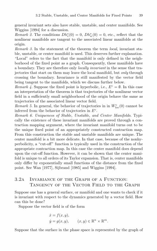
3.2 Stable, Unstable, and Center Manifolds for Fixed Points 39
general invariant sets also have stable, unstable, and center manifolds. SeeWiggins [1994] for a discussion.Remark 2. The conditions Dhs
v(0) = 0, Dhsw(0) = 0, etc., reflect that the
nonlinear manifolds are tangent to the associated linear manifolds at theorigin.Remark 3. In the statement of the theorem the term local, invariant sta-ble, unstable, or center manifold is used. This deserves further explanation.“Local” refers to the fact that the manifold is only defined in the neigh-borhood of the fixed point as a graph. Consequently, these manifolds havea boundary. They are therefore only locally invariant in the sense that tra-jectories that start on them may leave the local manifold, but only throughcrossing the boundary. Invariance is still manifested by the vector fieldbeing tangent to the manifolds, which we discuss further below.Remark 4. Suppose the fixed point is hyperbolic, i.e., Ec = ∅. In this casean interpretation of the theorem is that trajectories of the nonlinear vectorfield in a sufficiently small neighborhood of the origin behave the same astrajectories of the associated linear vector field.Remark 5. In general, the behavior of trajectories in in W c
loc(0) cannot beinferred from the behavior of trajectories in Ec.Remark 6. Uniqueness of Stable, Unstable, and Center Manifolds. Typi-cally the existence of these invariant manifolds are proved through a con-traction mapping argument, where the invariant manifold turns out to bethe unique fixed point of an appropriately constructed contraction map.From this construction the stable and unstable manifolds are unique. Thecenter manifold is a bit more delicate. In that case, because of the nonhy-perbolicity, a “cut-off” function is typically used in the construction of theappropriate contraction map. In this case the center manifold does dependupon the cut-off function. However, it can be shown that the center mani-fold is unique to all orders of its Taylor expansion. That is, center manifoldsonly differ by exponentially small functions of the distance from the fixedpoint. See Wan [1977], Sijbrand [1985] and Wiggins [1994].
3.2a Invariance of the Graph of a Function:Tangency of the Vector Field to the Graph
Suppose one has a general surface, or manifold and one wants to check if itis invariant with respect to the dynamics generated by a vector field. Howcan this be done?
Suppose the vector field is of the form
x = f(x, y),y = g(x, y), (x, y) ∈ R
n × Rm.
Suppose that the surface in the phase space is represented by the graph of
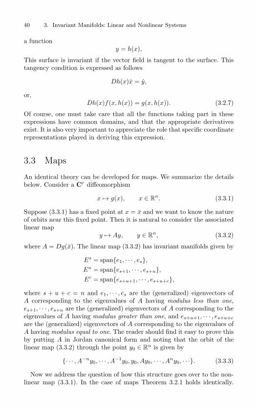
40 3. Invariant Manifolds: Linear and Nonlinear Systems
a functiony = h(x),
This surface is invariant if the vector field is tangent to the surface. Thistangency condition is expressed as follows
Dh(x)x = y,
or,Dh(x)f(x, h(x)) = g(x, h(x)). (3.2.7)
Of course, one must take care that all the functions taking part in theseexpressions have common domains, and that the appropriate derivativesexist. It is also very important to appreciate the role that specific coordinaterepresentations played in deriving this expression.
3.3 Maps
An identical theory can be developed for maps. We summarize the detailsbelow. Consider a Cr diffeomorphism
x → g(x), x ∈ Rn. (3.3.1)
Suppose (3.3.1) has a fixed point at x = x and we want to know the natureof orbits near this fixed point. Then it is natural to consider the associatedlinear map
y → Ay, y ∈ Rn, (3.3.2)
where A = Dg(x). The linear map (3.3.2) has invariant manifolds given by
Es = spane1, · · · , es,Eu = spanes+1, · · · , es+u,Ec = spanes+u+1, · · · , es+u+c,
where s + u + c = n and e1, · · · , es are the (generalized) eigenvectors ofA corresponding to the eigenvalues of A having modulus less than one,es+1, · · · , es+u are the (generalized) eigenvectors of A corresponding to theeigenvalues of A having modulus greater than one, and es+u+1, · · · , es+u+c
are the (generalized) eigenvectors of A corresponding to the eigenvalues ofA having modulus equal to one. The reader should find it easy to prove thisby putting A in Jordan canonical form and noting that the orbit of thelinear map (3.3.2) through the point y0 ∈ R
n is given by
· · · , A−ny0, · · · , A−1y0, y0, Ay0, · · · , Any0, · · ·. (3.3.3)
Now we address the question of how this structure goes over to the non-linear map (3.3.1). In the case of maps Theorem 3.2.1 holds identically.
3.4 Some Examples 41
FIGURE 3.3.1. Local invariant manifold structure in the unforced Duffing oscil-
lator, 0 < δ <√
8.
Namely, the nonlinear map (3.3.1) has a Cr invariant s-dimensional sta-ble manifold, a Cr invariant u-dimensional unstable manifold, and a Cr
invariant c-dimensional center manifold all intersecting in the fixed point.Moreover, these manifolds are all tangent to the respective invariant man-ifolds of the linear map (3.3.2) at the fixed point.
Essentially, everything about stable, unstable, and center manifolds forfixed points of vector fields holds for fixed points of maps. We will giveexamples in the exercises. However, before completing our discussion of in-variant manifolds let us apply our results to the unforced Duffing oscillator.
3.4 Some Examples
Example 3.4.1 (Application to the Unforced Duffing Oscillator). In Section 1
we have seen that the equation
x = y,
y = x − x3 − δy, δ > 0,
has a saddle-type fixed point of (x, y) = (0, 0), and sinks at (±1, 0) for δ > 0. From
Theorem 3.2.1 we now know that (±1, 0) have two-dimensional stable manifolds
(this is obvious) and (0, 0) has a one-dimensional stable manifold and a one-
dimensional unstable manifold as shown in Figure 3.3.1 (note: we have drawn
the figure for 0 < δ <√
8. The reader should show how the solutions near the
sinks are modified for δ >√
8). Note that Theorem 3.2.1 also tells us that a good
local approximation to the stable and unstable manifolds of (0, 0) is given by the
corresponding invariant linear manifolds, which are relatively easy to calculate.
The case δ = 0 is treated in great detail in Chapter 5.
End of Example 3.4.1
42 3. Invariant Manifolds: Linear and Nonlinear Systems
Let us consider a final example from Guckenheimer and Holmes [1983].
FIGURE 3.4.1. The stable and unstable subspaces in Example 3.4.2.
Example 3.4.2. Consider the planar vector field
x = x,
y = −y + x2, (x, y) ∈ R1 × R
1,
which has a hyperbolic fixed point at (x, y) = (0, 0). The associated linearized
system is given by
x = x,
y = −y,
with stable and unstable subspaces given by
Es= (x, y) ∈ R
2 | x = 0 ,
Eu= (x, y) ∈ R
2 | y = 0 (see Figure 3.4.1).
Now we turn our attention to the nonlinear vector field for which, in this
case, the solution can be obtained explicitly as follows. Eliminating time as the
independent variable gives
y
x=
dy
dx=
−y
x+ x,
which can be solved to obtain
y(x) =x2
3+
c
x,
where c is some constant. Now W uloc(0, 0) can be represented by a graph over
the x variables, i.e., y = h(x) with h(0) = h′(0) = 0. Varying c in the solution
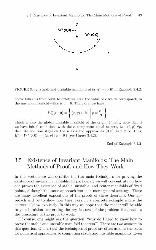
3.5 Existence of Invariant Manifolds: The Main Methods of Proof 43
FIGURE 3.4.2. Stable and unstable manifolds of (x, y) = (0, 0) in Example 3.4.2.
above takes us from orbit to orbit; we seek the value of c which corresponds to
the unstable manifold—this is c = 0. Therefore, we have
W uloc(0, 0) =
(x, y) ∈ R
2
∣∣∣∣∣ y =x2
3
,
which is also the global unstable manifold of the origin. Finally, note that if
we have initial conditions with the x component equal to zero, i.e., (0, y) ∀y,
then the solution stays on the y axis and approaches (0, 0) as t ↑ ∞; thus,
Es = W s(0, 0) = (x, y) | x = 0 (see Figure 3.4.2).
End of Example 3.4.2
3.5 Existence of Invariant Manifolds: The MainMethods of Proof, and How They Work
In this section we will describe the two main techniques for proving theexistence of invariant manifolds. In particular, we will concentrate on howone proves the existence of stable, unstable, and center manifolds of fixedpoints, although the same approach works in more general settings. Thereare many excellent expositions of the proofs of these theorems. Our ap-proach will be to show how they work in a concrete example where theanswer is know explicitly. In this way we hope that the reader will be ableto gain intuition concerning the key features of the problem that enablesthe procedure of the proof to work.
Of course, one might ask the question, “why do I need to know how toprove the stable and unstable manifold theorem?” There are two answers tothis question. One is that the techniques of proof are often used as the basisfor numerical approaches to computing stable and unstable manifolds. Even
44 3. Invariant Manifolds: Linear and Nonlinear Systems
if one has no interest in the details of the proof of the theorem, in using itin applications one often needs to numerically compute the manifolds. Anoverview of such numerical methods can be found in Moore and Hubert[1999] and Osinga [1996]. The other answer is that in a specific applicationthe precise setting or hypotheses of the theorem may not be satisfied (e.g.,the equilibrium point may be a saddle, but not hyperbolic, or the invariantset may be more complicated than an equilibrium point). In this situationit may be possible to prove a new theorem by following the same generalapproach, but with modifying certain details.
The main techniques for proving the existence of invariant manifolds arethe following.
Hadamard’s Method-The Graph Transform
Hadamard [1901] developed this method to prove the existence of stableand unstable manifolds of a fixed point of a Cr invertible map. The graphtransform method is more geometrical in nature than the Liapunov-Perronmethod. In the context of a hyperbolic fixed point, the stable and unstablemanifolds are constructed as graphs over the linearized stable and unstablesubspaces, respectively–hence the name. Fenichel [1971], [1974], [1977] andHirsch, Pugh, and Shub [1978] used this method in obtaining their generalresults on normally hyperbolic invariant manifolds. An elementary and de-tailed exposition of the graph transform method following Fenichel can befound in Wiggins [1994].
The Liapunov- Perron Method
Perron [1928], [1929], [1930] and Liapunov [1947] developed a methodfor proving the existence of stable and unstable manifolds of a hyperbolicequilbrium point. It deals with the integral equation formulation of theordinary differential equations and constructs the invariant manifolds as afixed point of an operator that is derived from this integral equation on afunction space whose elements have the appropriate interpretation as sta-ble and unstable manifolds. The Liapunov-Perron method has been used inmany different situations. The book of Hale [1980] is a good reference pointfor surveying these applications. In this book Hale surveys the fundamen-tal earlier work of Krylov and Bogoliubov, Bogoliubov and Mitropolski,Diliberto, Kyner, Kurzweil, and Pliss. In Chapter 7 of Hale [1980] severaltheorems related to various aspects of invariant manifolds are given whichwe refer to collectively as the “Hale invariant manifold theorem”. Theseresults can be viewed as a generalization and extension of much of the ear-lier work. Much of this work has recently been generalized in Yi [1993a,b].Chicone [1999] has an excellent elementary and detailed exposition of theLiapunov-Perron method.
3.5 Existence of Invariant Manifolds: The Main Methods of Proof 45
3.5a Application of These Two Methods to aConcrete Example: Existence of theUnstable Manifold
We recall Example 3.4.2:
x = x,
y = −y + x2, (x, y) ∈ R2. (3.5.1)
This vector field has a hyperbolic fixed point at the origin with unstablemanifold given by
y =x2
3. (3.5.2)
Now we will prove the existence of the unstable manifold by the graphtransform method and the Liapunov-Perron method.
Application of the Graph Transform Method
The trajectory of (3.5.1) through the point (x0, y0) at t = 0 is easily calcu-lated and found to be:
x(t;x0, y0) = x0et,
y(t;x0, y0) = y0e−t +
13x2
0e−t
(e3t − 1
). (3.5.3)
We view the trajectories as mapping initial conditions at t = 0 to pointsat the time t; often this is referred to as the time-t map.
Now consider a function y = h(x), and we consider an initial condition(x0, y0) on the graph of this function, i.e., y0 = h(x0). The image of thisinitial condition under the time-t map is given by
(x0, h(x0)) → (x(t;x0, h(x0)), y(t;x0, h(x0))) . (3.5.4)
Now if the graph of y = h(x) was an invariant manifold then, for any t, wewould have:
y(t;x0, h(x0)) = h(x(t;x0, h(x0))). (3.5.5)
This motivates us to define the following graph transform, G:
Gh (x(t;x0, h(x0))) = y(t;x0, h(x0)), (3.5.6)
where from (3.5.5) we see that the graph of a function y = h(x) is invariantunder the time-t map if it is a fixed point of the graph transform.
Now we are getting ahead of ourselves and we need to go back anddevelop the mathematical setting where the phrase “fixed point of thegraph transform” makes sense.
46 3. Invariant Manifolds: Linear and Nonlinear Systems
We define the following space of functions:
Sδ ≡ the set of functions, h(x),where |h(x)− h(x′)| ≤ δ|x− x′|,|x| ≤ ε, δ > 0 .
(3.5.7)In other words, these are the set of Lipshitz functions with Lipschitz con-stant δ defined on the domain |x| ≤ ε. These two parameters, δ and ε areadjusted in order to make the proof work. We can put a norm on Sδ thatis defined as follows:
‖ h ‖≡ sup|x|≤ε
|h(x)|.
With this norm Sδ becomes a Banach space, but more importantly, itbecomes a complete metric space in the metric that is defined by this norm.This latter fact is important for using the contraction mapping principle.
The complete metric space Sδ will be the domain on which the graphtransform is defined. Ultimately, we want to show that the graph transformhas a fixed point in Sδ which, as we argued above, will be an invariantmanifold. However first, several facts must be established.
The Graph Transform is Well-Defined:
We need to show that for any h ∈ Sδ, Gh is a function. Using (3.5.3) and(3.5.6), we have
Gh(x(t;x0, h(x0))) = h(x0)e−t +13x2
0e−t
(e3t − 1
).
Clearly, this is a well-defined function.
G : Sδ → Sδ:
This is the first step in showing that G is a contraction map on Sδ.First, we need a preliminary result. Define
ξ = x(t;x0, h(x0)) = x0et, ξ′ = x(t;x′
0, h(x′0)) = x′
0et.
Then, for t ≥ 0, we have
|ξ − ξ′| ≥ |x0 − x′0|. (3.5.8)
Next we calculate:
|Gh(ξ)− Gh(ξ′)| ≤ e−t|h(x0)− h(x′0)|+
13e−t
(e3t − 1
)|x0 + x′
0||x0 − x′0|,
≤(
δe−t +13e−t
(e3t − 1
)|x0 + x′
0|)|x0 − x′
0|,
≤(
δe−t +13e−t
(e3t − 1
)|x0 + x′
0|)|ξ − ξ′|,
≤(
δe−t +23e−t
(e3t − 1
)ε
)|ξ − ξ′| (3.5.9)
3.5 Existence of Invariant Manifolds: The Main Methods of Proof 47
Now for fixed t > 0, we can choose δ and ε small enough such that(δe−t +
23e−t
(e3t − 1
)ε
)≤ δ.
G is a Contraction Map on Sδ:
Choose x0 and x′0 such that
ξ = x(t;x0, h1(x0)) = x(t; x′0, h2(x′
0)). (3.5.10)
Since x(t;x0, h1(x0)) = x0et, x(t;x′
0, h2(x′0)) = x′
0et this implies that
x0 = x′0. (3.5.11)
Now for h1, h2 ∈ Sδ we have
|Gh1(ξ)− Gh2(ξ)| ≤ e−t|h1(x0)− h2(x0)|≤ e−t ‖ h1 − h2 ‖, (3.5.12)
which is a contraction for t > 0. Therefore by the contraction mappingtheorem, the graph transform has a unique fixed point, h(x), |x| ≤ ε. Byconstruction, the graph of h(x) is invariant under the time-t map, for somefixed t > 0.
y = h(x) is Invariant:
There are two important points that need to be addressed related to theissue of invariance.
We have argued that y = h(x) is invariant under the discrete time-t map,for some fixed t > 0. 1 There is a technicality involved with this statement.One sees from the form of the trajectories of the vector field given in (3.5.3)that the x component of any trajectory grows exponentially in time. Thatmeans that any point starting on y = h(x) will eventually leave y = h(x)(for t > 0), but only by crossing the boundary, which is given by the twopoints y+ = h(+ε) and y− = h(−ε). The graph of h(x) is an exampleof a locally invariant manifold. That is, points starting on the graph ofh(x) remain on the graph during time evolution, except they may leave
1Notice that the subscript “0” has disappeared from x0 in our notation forthe domain of the graph of the function which gives the local unstable manifold.This seemingly trivial point is one worth considering in a bit more detail. Thesubscript “0” makes explicit the fact that the invariant manifolds are manifolds ofinitial conditions for trajectories. This understanding is important and is similarto the understanding of how trajectories are different from orbits. Once this ismade clear, the subscript “0” can be dropped since initial conditions are justpoints in the phase space. However, in setting up the problem, one needs to havethe subscript so as not to confuse the notation for the initial condition with thatfor the trajectory itself.
48 3. Invariant Manifolds: Linear and Nonlinear Systems
the graph but only by crossing the boundary. This situation is typical forlocal stable, unstable, and center manifolds associated with fixed pointssince these manifolds are constructed in small neighborhoods of the fixedpoint as graphs over the respective linearized stable, unstable, and centersubspaces. Therefore the domains of the graphs are finite, which generallygives rise to a boundary for these local invariant manifolds. Shortly wewill show how one turns these local manifolds into global manifolds (anddescribe what that means).
The second important point concerning invariance is that we need toestablish that points that start on y = h(x) stay on it for any time, unlessthey leave it by crossing the boundary. Our graph transform proof has onlyshown that the graph of h(x) is invariant with respect to the time-t map forsome fixed t > 0. We leave the details of this as an exercise for the reader,but see Hartman [1964], Fenichel [1971], or Wiggins [1994] for details.
Continuation: The Global Unstable Manifold:
Once the existence of the local unstable manifold is established, we canthen construct the global unstable manifold by letting the local unstablemanifold evolve in time under the time-t map. More precisely, the globalunstable manifold of the origin is given by:
Wu ≡⋃t≥0
|x|≤ε
(x(t;x, h(x)), y(t;x, h(x))
). (3.5.13)
Clearly, this is object is invariant since it is a union of trajectories. It is alsoone dimensional, and trajectories with initial conditions in Wu approachthe origin at an exponential rate as t → −∞.
Differentiability of the Unstable Manifold:
The local unstable manifold found by the graph transform is the graph ofa Lipschitz function. However, the stable, unstable, and center manifoldtheorem for a fixed point states that if the vector field (or map) is Cr, thenthe unstable manifold should also be Cr (and our example is C∞).
The procedure for showing that y = h(x) is C1 is as follows. The fixedpoint of the graph transform satisfies (3.5.5). We formally differentiate(3.5.5) with respect to x0 to obtain:
Dh(D1x + D2x Dh
)= D1y + D2y Dh,
orDh =
(D1y + D2y Dh
) (D1x + D2x Dh
)−1. (3.5.14)
Here we are leaving out the arguments of all the functions in (3.5.5). Thenotation D denotes the derivative with respect to x0, D1 denotes the partialderivative with respect to x0 and D2 denotes the partial derivative with
3.5 Existence of Invariant Manifolds: The Main Methods of Proof 49
respect to y0. The phrase “formally differentiate’ used above means to doexactly what we did to (3.5.5), which resulted in (3.5.14). We do not knowthat (3.5.14) has any meaning since it has not yet been shown that h(x) isdifferentiable.
Therefore we define the operator
Hv ≡ (D1y + D2y v) (D1x + D2x v)−1, (3.5.15)
where v(·) is the unknown function. Clearly, a fixed point of this operator isa solution of (3.5.14). We use contraction mapping techniques to show thatH does have a fixed point. Then we show that this fixed point is actuallythe derivative of the fixed point of the graph transform. This will show thatthe fixed point of the graph transform is C1. One then proceeds inductivelyto obtain higher order derivatives. The details can be found in Hartman[1964], Fenichel [1971], or Wiggins [1994].
This approach yields that the local unstable manifold is differentiable.What about the global unstable manifold defined in (3.5.13)? This willfollow from Theorem 7.1.1 in Chapter 7 which says that the trajectories ofa Cr vector field are Cr functions of the initial conditions. Since (3.5.13) isconstructed by mapping the initial conditions of the local unstable manifoldby the trajectories it will then follow that the global unstable manifold isCr.
Application of the Liapunov-Perron Method
Now we develop the Liapunov-Perron method for proving the existence ofthe unstable manifold of the origin for the same example. The Liapunov-Perron method uses the integral equation form of the ordinary differentialequation (3.5.1), since (3.5.1) can be equivalently written in the form:
x(t;x0, y0) = x0et,
y(t;x0, y0) = y0e−t + e−t
∫ t
0eτx2(τ ;x0, y0)dτ. (3.5.16)
Suppose the graph of a Lipschitz function y = h(x), with h(0) = 0 andLipschitz constant δ, is an invariant set for (3.5.1). Then y(t;x0, h(x0)) =h(x(t; x0, h(x0))) is a solution of
y = −y + x2, (3.5.17)
with y(0;x0, h(x0)) = h(x0). Using (3.5.16), (3.5.17) can be rewritten as
y(t;x0, h(x0)) = h(x0)e−t + e−t
∫ t
0eτx2(τ ;x0, h(x0))dτ, (3.5.18)
or
h(x0) = ety(t;x0, h(x0))−∫ t
0eτx2(τ ; x0, h(x0))dτ. (3.5.19)
50 3. Invariant Manifolds: Linear and Nonlinear Systems
Now
|y(t;x0, h(x0))| = |h(x(t;x0, h(x0)))| ≤ δ|x(t;x0, h(x0))| = δet|x0|,
from which it follows that
limt→−∞
ety(t;x, h(x)) = 0.
Therefore, taking the limit as t → −∞ in (3.5.19) gives:
h(x0) =∫ 0
−∞eτx2(τ ;x0, h(x0))dτ, (3.5.20)
=∫ 0
−∞eτx2
0e2τdτ =
x20
3,
which is exactly the unstable manifold of the origin. Conversely, one canshow that if h(x0) satisfies (3.5.20), then the graph of y = h(x) is invariant.
This motivates the following definition of the Liapunov-Perron operator:
Ph(x0) =∫ 0
−∞eτx2(τ ;x0, h(x0))dτ, (3.5.21)
which is defined on the complete metric space
S0δ ≡ the set of functions, h(x),where |h(x)− h(x′)| ≤ δ|x− x′|,
h(0) = 0, |x| ≤ ε, δ > 0 ,(3.5.22)
with metric derived from the following norm
‖ h ‖≡ sup|x|≤ε
|h(x)|.
By our construction, a fixed point of the Liapunov-Perron operator is theunstable manifold of the origin. We will show that the Liapunov- Perronoperator is a contraction map on S0
δ . As for the graph transform, severalsteps must be carried out in the course of establishing this fact. Of course,all of this is unneccessary for this example since we have already foundthe fixed point for the Liapunov- Perron operator, which is exactly theglobal unstable manifold of the origin. However, our goal here is to givea description of the method in general. With that in mind, we proceedaccordingly.
P is Well-Defined:
This is obvious for this example from the form of (3.5.21).
3.5 Existence of Invariant Manifolds: The Main Methods of Proof 51
P : S0δ → S0
δ :
Using (3.5.21) and the first equation of (3.5.16), we have
|Ph(x0)− Ph(x′0)| ≤
13|x0 + x′
0| |x0 − x′0| ≤
2ε
3|x0 − x′
0|, (3.5.23)
so we need only choose ε small enough such that 2ε3 ≤ δ.
P is a Contraction Map on S0δ :
Using (3.5.21) and the first equation of (3.5.16), we have
|Ph1(x0)− Ph2(x0)| = 0, (3.5.24)
So P is clearly a contraction map. By the contraction mapping theoremit therefore has a unique fixed point whose graph (by construction) is theinvariant, local unstable manifold of the origin.
Once the existence of the local unstable manifold is established then itcan be continued to a global unstable manifold in the same way as wasdone for the local unstable manifold obtained by the graph transform. Itcan also be shown that the unstable manifold is differentiable in a waythat was similar to that described for the graph transform. That is, oneformally differentiates the Lipaunov-Perron operator and derives equationsthat the derivatives must satisfy. Fixed point methods are then use to showthat these equations have solutions, and that the solutions are indeed thederivatives. See Chicone [1999] for details.
Computing Invariant Manifolds using Taylor Expansions
Once we know the existence of a Cr invariant manifold we can use Tay-lor series methods to compute it. We will illustrate this in the context ofexample (3.5.1). Suppose the graph of y = h(x) is an invariant manifold.Then
y = Dh(x)x, (3.5.25)
orDh(x)x− y = 0. (3.5.26)
Since h(0) = 0 (the invariant manifold passes through the fixed points atthe origin) and Dh(0) = 0 (the invariant manifold is tangent to the unstablesubspace of the origin, i.e., the x-axis), we can assume that h(x) has thefollowing form (provided the vector field is at least C5, but our example isC∞):
y = h(x) = ax2 + bx3 + cx4 + · · · . (3.5.27)
Substituting the expression for x and y from (3.5.1) into (3.5.26) gives:
Dh(x)x−(−h(x) + x2) = 0. (3.5.28)
52 3. Invariant Manifolds: Linear and Nonlinear Systems
Substituting (3.5.27) into (3.5.28) gives(2ax2 + 3bx3 + 4cx4 +O(5)
)+ ax2 + bx3 + cx4 +O(5)− x2 = 0 (3.5.29)
In order to solve this equation the coefficient multiplying each power of xmust be zero. This implies:
x2 : 2a + a− 1 = 0⇒ a = 13
x3 : 3b + b = 0 ⇒ b = 0x4 : 4c + c = 0 ⇒ c = 0
In fact, one easily sees that the coefficient on the nth order term, for anyn > 2, must be zero. Hence we have
y = h(x) =x2
3.
Simo [1990] and Beyn and Kless [1998] show how the Taylor method canbe numerically implemented for computing invariant manifolds.
3.6 Time-Dependent Hyperbolic Trajectories andtheir Stable and Unstable Manifolds
In the previous sections we described the notion of hyperbolicity of a fixedpoint of an autonomous vector field, as well as the existence of stable, un-stable, and center manifolds associated with a fixed point (a parallel theoryfor maps also exists, but at the moment we are considering the continuoustime case of vector fields). All of these ideas and results were a result of thebehavior of the vector field linearized about the fixed point. More precisely,they followed from the eigenvalue and generalized eigenspace structure ofthe constant matrix associated with the linearized vector field. Now wewant to consider a general time dependent trajectory. What does it meanfor such a trajectory to be hyperbolic? Does a hyperbolic trajectory havestable and unstable manifolds? These are questions that we now address.
We consider vector fields of the form
x = f(x, t), x ∈ U ⊂ Rn, t ∈ R, (3.6.1)
where U is some open set in Rn.
The basic existence and uniqueness results for particle trajectories to or-dinary differential equations do not require very stringent requirements onthe time dependence (these will be discussed in detail in Chapter 7) ; con-tinuity in t is sufficient (see Hale [1980]). However, the dependence on x ismore stringent. We describe this more precisely in the following assumptionthat will stand throughout this chapter, unless otherwise stated.
3.6 Time-Dependent Hyperbolic Trajectories 53
Regularity Assumptions
We assume that f(x, t) is continuous in t, for all t ∈ R, and Cr in x, r ≥ 1.Moreover, all of the partial derivatives of v(x, t), with respect to x, up to
order r, are uniformly continuous and uniformly bounded in K×R, where Kis an arbitrary, compact subset of U . These “regularity assumptions” on the
velocity field will be sufficient for the invariant manifold theorems described
below (Coddington and Levinson [1955], Hale [1980], or Yi [1993a,b]).
3.6a Hyperbolic TrajectoriesWe have seen that if the matrix associated with the linearization about atrajectory is time dependent, then the eigenvalues of this matrix need notgive information about local stability of the trajectory. The appropriatenotion for characterizing the local (linearized) behavior in this case is that ofan exponential dichotomy (although Liapunov exponents are also relevant,which we will mention later), which we now define, and for which thestandard reference is Coppel [1978].
Definition 3.6.1 (Exponential Dichotomy) Consider the following lin-
ear ordinary differential equation with time dependent coefficients
ξ = A(t)ξ, ξ ∈ Rn, (3.6.2)
where A(t) is a continuous function of t ∈ R. Suppose X(t) is the fun-damental solution matrix of (3.6.2), i.e., for any initial condition ξ0,
ξ(t) = X(t)ξ0 is the solution of (3.6.2) passing through ξ0 at t = 0,X(0) = id. Let ‖ · ‖ denote a norm on R
n. Then (3.6.2) is said to possess
an exponential dichotomy if there exists a projection operator P , P 2 = P ,
and constants K1, K2, λ1, λ2 > 0, such that
‖ X(t)PX−1(τ) ‖ ≤ K1 exp (−λ1(t− τ)) , t ≥ τ, (3.6.3)‖ X(t) (id− P ) X−1(τ) ‖ ≤ K2 exp (λ2(t− τ)) , t ≤ τ. (3.6.4)
We now give a simple example of a linear autonomous vector field thatillustrates this notion of exponential dichotomy. In this case we know thatthe eigenvalues of the matrix used to define the linear vector field give usinformation about the local stability. Therefore one can relate this notionwith the new idea of an exponential dichotomy.
Example 3.6.1. Consider the following two dimensional, steady linear velocity
field:
x = −λx,
y = λy, (x, y) ∈ R2, λ > 0. (3.6.5)
54 3. Invariant Manifolds: Linear and Nonlinear Systems
The fundamental solution matrix is given by
X(t) =
(e−λt 0
0 eλt
)(3.6.6)
and we take
P =
(1 0
0 0
).
(Clearly, P 2 = P .) Then we have
X(t)PX−1(τ) =
(e−λ(t−τ) 0
0 0
),
and
X(t) (id − P ) X−1(τ) =
(0 0
0 eλ(t−τ)
).
We can take as a norm on the set of real 2 × 2 matrices the absolute value of the
largest matrix element. In that case we see that the bounds given in (3.6.1) are
obeyed for any K1 = K2 > 1.
End of Example 3.6.1
We now consider a less trivial time-dependent example.
Example 3.6.2.Consider the following linear vector field with time-periodic coefficients that
was earlier considered in Example 1.2.1:(x1
x2
)= A(t)
(x1
x2
),
where
A(t) =
( −1 + 32 cos2 t 1 − 3
2 cos t sin t−1 − 3
2 cos t sin t −1 + 32 sin2 t
). (3.6.7)
This is an example that we have seen earlier. The eigenvalues of A(t) are found
to be independent of t and are given by
λ1(t) =−1 + i
√7
4, λ2(t) =
−1 − i√
7
4.
In particular, they have negative real parts for all t. However, one can verify that
the following are two linearly independent solutions of this equation
v1(t) =
(− cos tsin t
)e
t2 , v2(t) =
(sin tcos t
)e−t. (3.6.8)
Therefore the fundamental solution matrix is given by:
X(t) =
(−e
t2 cos t e−t sin t
et2 sin t e−t cos t
), (3.6.9)
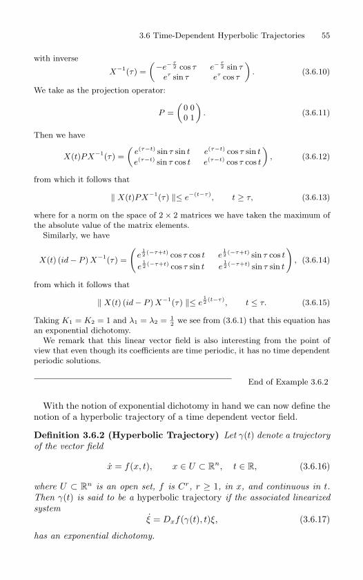
3.6 Time-Dependent Hyperbolic Trajectories 55
with inverse
X−1(τ) =
(−e− τ2 cos τ e− τ
2 sin τeτ sin τ eτ cos τ
). (3.6.10)
We take as the projection operator:
P =
(0 0
0 1
). (3.6.11)
Then we have
X(t)PX−1(τ) =
(e(τ−t) sin τ sin t e(τ−t) cos τ sin t
e(τ−t) sin τ cos t e(τ−t) cos τ cos t
), (3.6.12)
from which it follows that
‖ X(t)PX−1(τ) ‖≤ e−(t−τ), t ≥ τ, (3.6.13)
where for a norm on the space of 2 × 2 matrices we have taken the maximum of
the absolute value of the matrix elements.
Similarly, we have
X(t) (id − P ) X−1(τ) =
(e
12 (−τ+t) cos τ cos t e
12 (−τ+t) sin τ cos t
e12 (−τ+t) cos τ sin t e
12 (−τ+t) sin τ sin t
), (3.6.14)
from which it follows that
‖ X(t) (id − P ) X−1(τ) ‖≤ e
12 (t−τ), t ≤ τ. (3.6.15)
Taking K1 = K2 = 1 and λ1 = λ2 = 12 we see from (3.6.1) that this equation has
an exponential dichotomy.
We remark that this linear vector field is also interesting from the point of
view that even though its coefficients are time periodic, it has no time dependent
periodic solutions.
End of Example 3.6.2
With the notion of exponential dichotomy in hand we can now define thenotion of a hyperbolic trajectory of a time dependent vector field.
Definition 3.6.2 (Hyperbolic Trajectory) Let γ(t) denote a trajectory
of the vector field
x = f(x, t), x ∈ U ⊂ Rn, t ∈ R, (3.6.16)
where U ⊂ Rn is an open set, f is Cr, r ≥ 1, in x, and continuous in t.
Then γ(t) is said to be a hyperbolic trajectory if the associated linearized
system
ξ = Dxf(γ(t), t)ξ, (3.6.17)
has an exponential dichotomy.
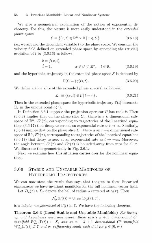
56 3. Invariant Manifolds: Linear and Nonlinear Systems
We give a geometrical explanation of the notion of exponential di-chotomy. For this, the picture is more easily understood in the extended
phase space:E ≡ (x, t) ∈ R
n × R |x ∈ U , (3.6.18)
i.e., we append the dependent variable t to the phase space. We consider thevelocity field defined on extended phase space by appending the (trivial)evolution of t to (3.6.16) as follows
x = f(x, t),t = 1, x ∈ U ⊂ R
n, t ∈ R, (3.6.19)
and the hyperbolic trajectory in the extended phase space E is denoted by
Γ(t) = (γ(t), t) . (3.6.20)
We define a time slice of the extended phase space E as follows:
Στ ≡ (x, t) ∈ E | t = τ . (3.6.21)
Then in the extended phase space the hyperbolic trajectory Γ(t) intersectsΣτ in the unique point γ(τ).
In Definition 3.6.1 suppose the projection operator P has rank k. Then(3.6.3) implies that on the phase slice Στ , there is a k dimensional sub-space of R
n, Es(τ), corresponding to trajectories of the linearized equa-tions (3.6.17) that decay to zero at an exponential rate as t →∞. Similarly,(3.6.4) implies that on the phase slice Στ , there is an n−k dimensional sub-space of R
n, Eu(τ), corresponding to trajectories of the linearized equations(3.6.17) that decay to zero at an exponential rate as t → −∞. Moreover,the angle between Es(τ) and Eu(τ) is bounded away from zero for all τ .We illustrate this geometrically in Fig. 3.6.1.
Next we examine how this situation carries over for the nonlinear equa-tions.
3.6b Stable and Unstable Manifolds ofHyperbolic Trajectories
We can now state the result that says that tangent to these linearizedeigenspaces we have invariant manifolds for the full nonlinear vector field.
Let Dρ(τ) ∈ Στ denote the ball of radius ρ centered at γ(τ). Then
Nρ (Γ(t)) ≡ ∪τ∈R (Dρ(τ), τ) ,
is a tubular neighborhood of Γ(t) in E . We have the following theorem.
Theorem 3.6.3 (Local Stable and Unstable Manifolds) For the set-
up and hypotheses described above, there exists k + 1 dimensional Cr
manifold W sloc(Γ(t)) ⊂ E, and an n − k + 1 dimensional Cr manifold
Wuloc(Γ(t)) ⊂ E and ρ0 sufficiently small such that for ρ ∈ (0, ρ0)
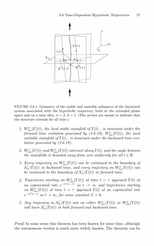
3.6 Time-Dependent Hyperbolic Trajectories 57
x2
1x
t
t
uE ( )s
E ( )t
FIGURE 3.6.1. Geometry of the stable and unstable subspaces of the linearized
system associated with the hyperbolic trajectory, both in the extended phase
space and on a time slice, n = 2, k = 1. (The arrows are meant to indicate that
the structure extends for all time.)
1. W sloc(Γ(t)), the local stable manifold of Γ(t) , is invariant under the
forward time evolution generated by (3.6.19), Wuloc(Γ(t)), the local
unstable manifold of Γ(t) , is invariant under the backward time evo-
lution generated by (3.6.19).
2. W sloc(Γ(t)) and Wu
loc(Γ(t)) intersect along Γ(t), and the angle between
the manifolds is bounded away from zero uniformly for all t ∈ R.
3. Every trajectory on W sloc(Γ(t)) can be continued to the boundary of
Nρ (Γ(t)) in backward time, and every trajectory on Wuloc(Γ(t)) can
be continued to the boundary of Nρ (Γ(t)) in forward time.
4. Trajectories starting on W sloc(Γ(t)) at time t = τ approach Γ(t) at
an exponential rate e−λ′(t−τ) as t → ∞ and trajectories starting
on Wuloc(Γ(t)) at time t = τ approach Γ(t) at an exponential rate
e−λ′|t−τ | as t →∞, for some constant λ′ > 0.
5. Any trajectory in Nρ (Γ(t)) not on either W sloc(Γ(t)) or Wu
loc(Γ(t))will leave Nρ (Γ(t)) in both forward and backward time.
Proof: In some sense this theorem has been known for some time, althoughthe autonomous version is much more widely known. The theorem can be
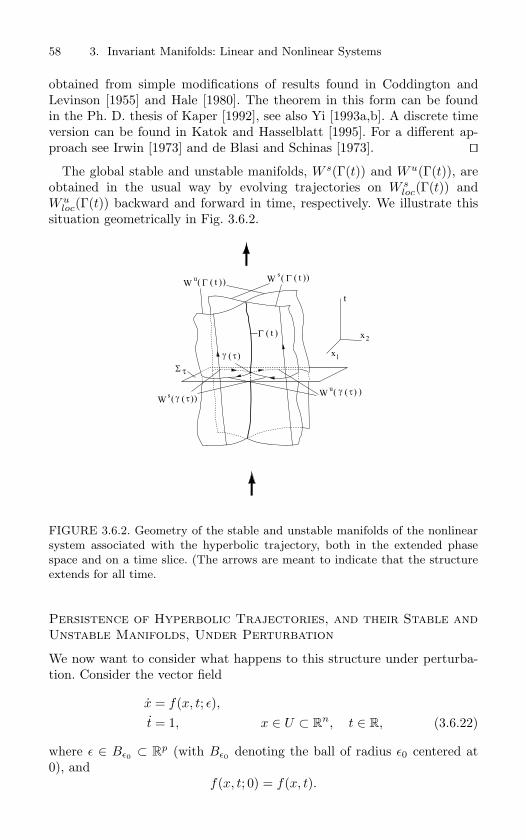
58 3. Invariant Manifolds: Linear and Nonlinear Systems
obtained from simple modifications of results found in Coddington andLevinson [1955] and Hale [1980]. The theorem in this form can be foundin the Ph. D. thesis of Kaper [1992], see also Yi [1993a,b]. A discrete timeversion can be found in Katok and Hasselblatt [1995]. For a different ap-proach see Irwin [1973] and de Blasi and Schinas [1973].
The global stable and unstable manifolds, W s(Γ(t)) and Wu(Γ(t)), areobtained in the usual way by evolving trajectories on W s
loc(Γ(t)) andWu
loc(Γ(t)) backward and forward in time, respectively. We illustrate thissituation geometrically in Fig. 3.6.2.
x2
1x
t
t
uW ( )
uW ( )t
s tW ( )
W ( )s
FIGURE 3.6.2. Geometry of the stable and unstable manifolds of the nonlinear
system associated with the hyperbolic trajectory, both in the extended phase
space and on a time slice. (The arrows are meant to indicate that the structure
extends for all time.
Persistence of Hyperbolic Trajectories, and their Stable andUnstable Manifolds, Under Perturbation
We now want to consider what happens to this structure under perturba-tion. Consider the vector field
x = f(x, t; ε),t = 1, x ∈ U ⊂ R
n, t ∈ R, (3.6.22)
where ε ∈ Bε0 ⊂ Rp (with Bε0 denoting the ball of radius ε0 centered at
0), andf(x, t; 0) = f(x, t).
3.7 Invariant Manifolds in a Broader Context 59
We assume that (3.6.22) depends upon the vector of parameters ε in a Cr
manner, with all of the partial derivatives of f(x, t, ε), with respect to ε, upto order r, being uniformly continuous and uniformly bounded in K × R,where K is an arbitrary, compact subset of R
p.
Theorem 3.6.4 (Persistence Under Perturbation) Suppose that at
ε = 0 Theorem 3.6.3 holds for (3.6.22). Then there exists ε0 sufficiently
small such that for all ε ∈ Bε0 (3.6.22) possesses a hyperbolic trajectory
Γε(t), having a k+1 dimensional stable manifold, W s(Γε(t)) and an n−k+1dimensional unstable manifold, Wu(Γε(t)). These manifolds have the same
properties as described in Theorem 3.6.3. Moreover, they depend on ε in a
Cr manner.
Proof: See Kaper [1992] or Yi [1993a,b]. An obvious question is how does one locate hyperbolic trajectories in
vector fields having a general time dependence? Theorem 3.6.4 provides uswith an easy way to do this if our problem is in the form of a time dependentperturbation of an autonomous vector field, i.e., consider a vector field ofthe form
x = f(x) + εg(x, t; ε),t = 1, x ∈ U ⊂ R
n, t ∈ R. (3.6.23)
Suppose that for ε = 0 the vector field x = v(x) has a hyperbolic fixed point.Then, by Theorem 3.6.4, for ε small this hyperbolic fixed point becomesa (generally) time varying hyperbolic trajectory with stable and unstablemanifolds.
3.7 Invariant Manifolds in a Broader Context
In this chapter the invariant manifolds of interest have been the stable,unstable, and center manifolds of fixed points. Invariant manifold theory isa much broader and deeper subject and in this section we wish to describesome of the issues associated with invariant manifolds in a broader context.
Existence of Invariant Manifolds
Invariant manifold theory begins by assuming that some “basic” invari-ant manifold exists–the theory is then developed from this point onwardsby building upon this basic invariant manifold. In particular, one is inter-ested in the construction of stable, unstable, and center manifolds asso-ciated with these basic invariant manifolds. The types of basic invariantmanifolds typically considered are:
1. Equilibrium points,
60 3. Invariant Manifolds: Linear and Nonlinear Systems
2. Periodic orbits,
3. Quasiperiodic or almost periodic orbits (invariant tori).
These manifolds all share an important property. Namely, they all admit aglobal coordinate description. In this case the dynamical system is typicallysubjected to a “preparatory” coordinate transformation that serves to lo-calize the dynamical system about the invariant manifold. This amounts toderiving a normal form in the neighborhood of an invariant manifold andit greatly facilitates the various estimates that are required in the analy-sis. Sacker [1969], Fenichel [1971], and Hirsch, Pugh, and Shub [1977] wereamong the first to consider general invariant manifolds that are not de-scribed as graphs and required an atlas of local coordinate charts for theirdescription. This is an important generalization since in recent years in-variant manifolds that cannot be expressed globally as a graph have arisenin applications, see Wiggins [1990], Hoveijn [1992], and Haller and Wiggins[1996] for applications where invariant spheres arise.
The Persistence and Differentiability of Invariant ManifoldsUnder Perturbation
The question of whether or not an invariant manifold persists under per-turbation and, if so, if it maintains, loses, or gains differentiabilty is alsoimportant. In considering these issues it is important to characterize thestability of the unperturbed invariant manifold. This is where the notionof normal hyperbolicity arises. Roughly speaking, a manifold is normallyhyperbolic if, under the dynamics linearized about the invariant manifold,the growth rate of vectors transverse to the manifold dominates the growthrate of vectors tangent to the manifold. For equilibrium points, these growthrates can be characterized in terms of eigenvalues associated with the lin-earization at the equilibria that are not on the imaginary axis, for periodicorbits these growth rates can be characterized in terms of the Floquet mul-tipliers associated with the linearization about the periodic orbit that arenot on the unit circle, for invariant tori or more general invariant manifoldsthese growth rates can be characterized in terms of exponential dichotomies(see Coppel [1978] or Sacker and Sell [1974]) or by the notion of generalizedLyapunov type numbers (Fenichel [1971]), which is the approach that wewill take in this book. A question of obvious importance for applicationsis how does one compute whether or not an invariant manifold is normallyhyperbolic? The answer is not satisfactory. For equilibria, the problem in-volves finding the eigenvalues of a square matrix–an algebraic problem. Forinvariant manifolds on which the dynamics is nontrivial the issues are morecomplicated, and they are dealt with in this book. However, one importantclass of dynamical systems which may have nontrivial invariant manifoldson which the dynamics is also nontrivial are integrable Hamiltonian sys-tems, see Wiggins [1988] for examples. Finally, we want to alert the reader
3.7 Invariant Manifolds in a Broader Context 61
to an important characteristic of normal hyperbolicity that is of some im-portance for understanding the scope of possible applications. Namely, it isinsensitive to the form of the dynamics on the invariant manifold, providedthe dynamics transverse to the invariant manifold is dominant in the senseof normal hyperbolicity. Heuristically, one could think of the dynamics onthe invariant manifold as being “slow” as compared to the “fast” dynamicsoff the invariant manifold. Hence, the dynamics on the invariant manifoldcould even be chaotic.
Characterizing growth rates in the fashion described above requiresknowledge of the linearized dynamics near orbits on the invariant man-ifold as t → +∞ or t → −∞. Hence, if the invariant manifold has aboundary (which an equilibrium point, periodic orbit, or invariant torusdoes not have), then one must understand the nature of the dynamics atthe boundary. Notions such as overflowing invariance or inflowing invari-
ance are developed to handle this. Invariant manifolds with boundary arisevery often in applications, see Wiggins [1988].
Behavior Near an Invariant Manifold–Stable, Unstable, andCenter Manifolds
A “stable manifold theorem” asserts that the set of points that approachan invariant manifold at an exponential rate as t → +∞ is an invariantmanifold in its own right. The exponential rate of approach is inherited fromthe linearized dynamics as the stable manifold is constructed as a graphover the linearized stable subspace or subbundle. An “unstable manifoldtheorem” asserts similar behavior in the limit as t → −∞. Obviously, onemay have problems with both of these concepts if the invariant manifoldhas a boundary.
The notion of a center manifold is more subtle. For equilibrium points andperiodic orbits a center manifold is an invariant manifold that is tangentto the linearized subspace corresponding to eigenvalues on the imaginaryaxis, and floquet multipliers on the unit circle, respectively. In contrast tothe situation with stable and unstable manifolds, the asymptotic behaviorof orbits in the nonlinear center manifold may be very different than theasymptotic behavior of orbits in the linearized center subspaces, under thelinearized dynamics.
Questions related to persistence and differentiability of stable, unstable,and center manifolds also arise.
More Refined Behavior Near Invariant Manifolds–Foliations ofStable, Unstable, and Center Manifolds
One may be interested in which orbits in the stable manifold approachthe invariant manifold at a specified rate. Under certain conditions theseorbits may lie on submanifolds of the stable manifold which are not in-variant, but make up an invariant family of submanifolds that foliate the
62 3. Invariant Manifolds: Linear and Nonlinear Systems
stable manifold. A similar situation may hold for the unstable manifold.Moreover, this foliation has the property that points in a fiber of the fo-liation asymptotically approach the trajectory in the invariant manifoldthat passes through the point of intersection of the fiber with the invariantmanifold (the basepoint of the fiber). This is a generalization of the notionof asymptotic phase, that is familiar from studies of stability of periodic or-bits, to arbitrary invariant manifolds. In recent years these foliations haveseen many uses in applications. Fenichel [1979] has used them in his de-velopment of geometric singular perturbation theory. Kovacic and Wiggins[1992], Haller and Wiggins [1993], [1995], and McLaughlin et al. [1996] haveused them in the development of new global perturbation methods. Finally,the recent monograph of Kirchgraber and Palmer [1990] proves a numberof foliation results and shows how these can be used as coordinates in whichthe dynamical system becomes linear.
Invariant Manifolds for Stochastic Dynamical Systems
Invariant manifold theory for stochastic, or random dynamical systemsis currently being developed. See Arnold [1998], Boxler [1989], [1991] andSchmalfuss [1998].
3.8 Exercises1. Prove that the boundary, closure, interior, and complement of an invariant set are
invariant.
2. Prove that the closure and interior of a positively invariant set are positively invariant.
3. Prove that the complement of a positively invariant set is negatively invariant.
4. Prove that the union and intersection of a family of invariant (resp. positively invariant)sets are invariant (resp. positively invariant).
5. Let x → f(x), x ∈ Rn, be a diffeomorphism and suppose x = 0 is a fixed point, i.e.,
f(0) = 0. We define the stable set of x = 0 as:
S ≡
y ∈ Rn | f
n(y) → 0, as n → ∞
.
Is S a manifold? (Be careful here, see McGehee [1973].)
6. Consider the linear vector field x = Ax, A a constant matrix.
(a) Verify that x(t) = eAtx0 is a trajectory of this vector field passing through thepoint x0 at t = 0.
(b) Prove uniqueness of solutions, i.e., verify that this is the only solution passingthrough x0 at t = 0.
(c) Describe the dependence of trajectories on initial conditions and time (e.g.,continuous, Cr, analytic, etc.).
(d) Suppose A depends on parameters., i.e., A = A(µ). Describe the dependence ofthe solutions on parameters in terms of the parameter dependence of A (e.g.,continuous, Cr, analytic, etc.).
(e) Show that x(t + τ) = eA(t+τ)x0 is also a solution, for any τ ∈ R. Does thisviolate uniqueness of solutions?
3.8 Exercises 63
(f) Prove that two different trajectories cannot intersect.
7. Prove that for any fixed t, the map
φt ≡ eAt : R
n → Rn
,
x → φt(x) ≡ eAt
x,
defines a diffeomorphism of Rn into R
n.
8. Prove that φt(x) ≡ eAtx satisfies the following properties:
(a) φ0(x) = x,
(b) φ−t φt(x) = x,
(c) φt φs(x) = φt+s(x),
for all t ∈ R, x ∈ Rn. A one-parameter family of diffeomorphisms satisfying these three
properties is said to be a flow, and we say that the solutions of the vector field x = Axdefine a flow on the phase space.
9. Prove that
V (A, λα,γ) ≡ Ker (A − λα,γ id)nα,γ , α = s, u, c, γ = i, k, m,
is an invariant (under A) subspace of Rn. Prove that it is also invariant under eAt.
10. Prove that FR is a real vector space.
11. Prove that EC is a complex subspace of Cn.
12. Prove that (EC)R
= E.
13. Suppose E ⊂ Rn is a subspace with basis
e1, . . . , ek ≡ e,
andA : E → E,
is a real linear map.
(a) Prove that e is also a basis for EC.
(b) Prove that the matrix representation of A with respect to e is the same as thematrix representation of AC with respect to e.
14. Let E be a real vector space and A a linear map of E into E. Show that
(a) (Ker )C
= Ker (AC),
(b) (Im A)C
= Im (AC),
(c)(A−1)
C= (AC)−1, if A is invertible.
In this exercise Ker denotes the kernel and Im denotes the image, or range.
15. Suppose A : E → E is a real linear map. Show that A and AC have the samecharacteristic polynomial.
16. Prove thatV (A, µα,γ , µα,γ) ,
is an invariant (under A) subspace of Rn. Prove that it is also invariant under eAt.

64 3. Invariant Manifolds: Linear and Nonlinear Systems
17. Prove that Es, Eu, and Ec, defined in (3.1.6), (3.1.7), and (3.1.8), respectively, areeach invariant under eAt.
(a) Prove that trajectories with initial conditions in Es approach zero at an expo-nential rate as t → ∞.
(b) Prove that trajectories with initial conditions in Eu approach zero at an expo-nential rate as t → −∞.
18. What can one say about trajectories with initial conditions in Ec under the followingconditions on the eigenvalues:
(a) there are no repeated eigenvalues,
(b) there are no zero eigenvalues,
(c) there are no zero eigenvalues, and no repeated eigenvalues.
19. Suppose that Ec = ∅. Prove that the only trajectories starting in a neighborhood ofthe origin that remain in that neighborhood for all time are those that start on Es.
20. The Variation of Constants Formula. Consider the following inhomogeneous linearordinary differential equation:
x = Ax + g(t), x ∈ Rn
,
where A is an n × n-matrix of real numbers. Verify that the solution of this equationpassing through x0 at t = 0 is given by
x(t) = eAt
∫ t
0e
−Asg(s)ds + e
Atx0.
Prove that this solution is unique. What conditions on g(t) are required for this uniquesolution to exist?
21. Consider the block diagonal form of the linear vector field given in (3.2.5). Relate thisblock diagonal form of the vector field to the decomposition of the phase space asR
n = Es ⊕ Eu ⊕ Ec.
22. Consider the following linear vector fields on R2.
a)(
x1x2
)=(
λ 00 µ
)(x1x2
),
λ < 0µ > 0 .
b)(
x1x2
)=(
λ 00 µ
)(x1x2
),
λ < 0µ < 0 .
c)(
x1x2
)=(
λ −ωω λ
)(x1x2
),
λ < 0ω > 0 .
d)(
x1x2
)=(
0 00 λ
)(x1x2
), λ < 0.
e)(
x1x2
)=(
0 λ0 0
)(x1x2
), λ > 0.
f)(
x1x2
)=(
0 00 0
)(x1x2
).
i. For each vector field compute all trajectories and illustrate them graphi-cally on the phase plane. Describe the stable, unstable, and center mani-folds of the origin.
ii. For vector field a), discuss the cases |λ| < µ, |λ| = µ, and |λ| > µ. What arethe qualitative and quantitative differences in the dynamics for these threecases? Can the unstable manifold of the origin be considered an attractingset and/or an attractor and do the relative magnitudes of the eigenvaluesaffect these conclusions?
3.8 Exercises 65
iii. For vector field b), discuss the cases λ < µ, λ = µ, λ > µ. What arethe qualitative and quantitative differences in the dynamics for these threecases? Describe all zero- and one-dimensional invariant manifolds for thisvector field. Describe the nature of the trajectories at the origin. In par-ticular, which trajectories are tangent to either the x1 or x2 axis?
iv. In vector field c), describe how the trajectories depend on the relativemagnitudes of λ and ω. What happens when λ = 0? When ω = 0?
v. Describe the effect of linear perturbations on each of the vector fields.vi. Describe the effect near the origin of nonlinear perturbations on each of
the vector fields. Can you say anything about the effects of nonlinear per-turbations on the dynamics outside of a neighborhood of the origin?
We remark that vi) is a difficult problem for the nonhyperbolic fixed points. We willstudy this situation in great detail when we develop center manifold theory and bifur-cation theory.
23. Give a characterization of the stable, unstable, and center subspaces for linear maps interms of generalized eigenspaces along the same lines as we did for linear vector fieldsaccording to the formulae (3.1.6), (3.1.7), and (3.1.8).
24. For the following linear vector fields find the general solution, and compute the stable,unstable, and center subspaces and plot them in the phase space.
a)(
x1x2
)=(
1 23 2
)(x1x2
)
b)
x1
x2x3
=
3 0 0
0 2 −50 1 −2
x1
x2x3
c)
x1
x2x3
=
1 −3 3
3 −5 36 −6 4
x1
x2x3
d)
x1
x2x3
=
−3 1 −1
−7 5 −1−6 6 −2
x1
x2x3
e)
x1
x2x3
=
1 0 0
1 2 01 0 −1
x1
x2x3
f)
x1
x2x3
=
1 0 1
0 0 −20 1 0
x1
x2x3
g)
x1
x2x3
=
0 0 15
1 0 −170 1 7
x1
x2x3
h)
x1
x2x3
=
0 0 1
0 1 20 3 2
x1
x2x3
25. Consider the following linear maps on R2.
a)(
x1x2
)→
(λ 00 µ
)(x1x2
),
|λ| < 1|µ| > 1 .
b)(
x1x2
)→
(λ 00 µ
)(x1x2
),
|λ| < 1|µ| < 1 .
c)(
x1x2
)→
(λ −ωω λ
)(x1x2
), ω > 0.
d)(
x1x2
)→
(1 00 λ
)(x1x2
), |λ| < 1.
66 3. Invariant Manifolds: Linear and Nonlinear Systems
e)(
x1x2
)→
(1 λ0 1
)(x1x2
), λ > 0.
f)(
x1x2
)→
(1 00 1
)(x1x2
).
i. For each map compute all the orbits and illustrate them graphically onthe phase plane. Describe the stable, unstable, and center manifolds of theorigin.
ii. For map a), discuss the cases λ, µ > 0; λ = 0, µ > 0; λ, µ < 0; and λ < 0,µ > 0. What are the qualitative differences in the dynamics for these fourcases? Discuss how the orbits depend on the relative magnitudes of theeigenvalues. Discuss the attracting nature of the unstable manifold of theorigin and its dependence on the relative magnitudes of the eigenvalues.
iii. For map b), discuss the cases λ, µ > 0; λ = 0, µ > 0; λ, µ < 0; and λ < 0,µ > 0. What are the qualitative differences in the dynamics for these fourcases? Describe all zero- and one-dimensional invariant manifolds for thismap. Do all orbits lie on invariant manifolds?
iv. For map c), consider the cases λ2 + ω2 < 1, λ2 + ω2 > 1, and λ + iω = eiα
for α rational and α irrational. Describe the qualitative differences in thedynamics for these four cases.
v. Describe the effect of linear perturbations on each of the maps.vi. Describe the effect near the origin of nonlinear perturbations on each of the
maps. Can you say anything about the effects of nonlinear perturbationson the dynamics outside of a neighborhood of the origin?
We remark that vi) is very difficult for nonhyperbolic fixed points (more so than theanalogous case for vector fields in the previous exercise) and will be treated in greatdetail when we develop center manifold theory and bifurcation theory.
26. Consider the following vector fields.
a) x = y,y = −δy − µx,
(x, y) ∈ R2.
b)x = y,y = −δy − µx − x2,
(x, y) ∈ R2.
c)x = y,y = −δy − µx − x3,
(x, y) ∈ R2.
d)x = −δx − µy + xy,y = µx − δy + 1
2 (x2 − y2), (x, y) ∈ R2.
e) x = −x + x3,y = x + y,
(x, y) ∈ R2.
f)r = r(1 − r2),θ = cos 4θ,
(r, θ) ∈ R+ × S
1.
g)r = r(δ + µr2 − r4),θ = 1 − r2,
(r, θ) ∈ R+ × S
1.
h) θ = v,v = − sin θ − δv + µ,
(θ, v) ∈ S1 × R.
i) θ1 = ω1,
θ2 = ω2 + θn1 , n ≥ 1,
(θ1, θ2) ∈ S1 × S
1.
j) θ1 = θ2 − sin θ1,
θ2 = −θ2,(θ1, θ2) ∈ S
1 × S1.
k) θ1 = θ21 ,
θ2 = ω2,(θ1, θ2) ∈ S
1 × S1.
Describe the nature of the stable and unstable manifolds of the fixed points by draw-ing phase portraits. Can you determine anything about the global behavior of themanifolds?
In a), b), c), d), g), and h) consider the cases δ < 0, δ = 0, δ > 0, µ < 0, µ = 0, andµ > 0. In i) and k) consider ω1 > 0 and ω2 > 0.
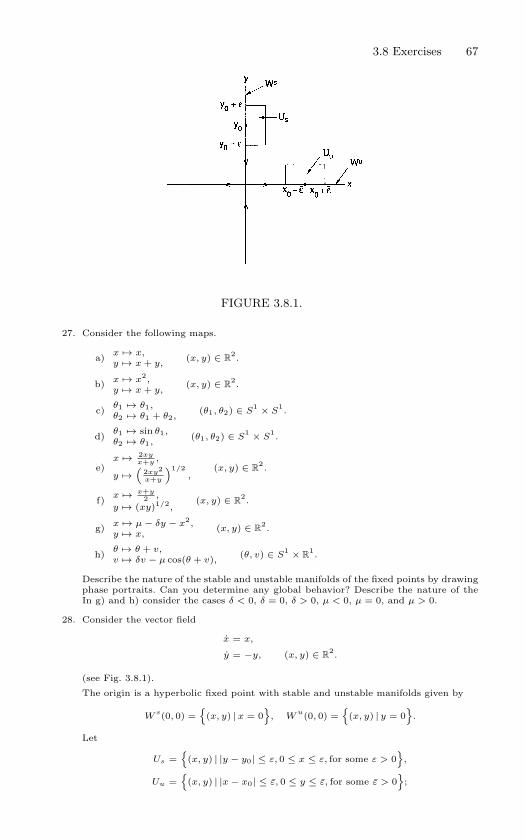
3.8 Exercises 67
FIGURE 3.8.1.
27. Consider the following maps.
a) x → x,y → x + y,
(x, y) ∈ R2.
b) x → x2,y → x + y,
(x, y) ∈ R2.
c) θ1 → θ1,θ2 → θ1 + θ2,
(θ1, θ2) ∈ S1 × S
1.
d) θ1 → sin θ1,θ2 → θ1,
(θ1, θ2) ∈ S1 × S
1.
e)x → 2xy
x+y ,
y →(
2xy2
x+y
)1/2,
(x, y) ∈ R2.
f) x → x+y2 ,
y → (xy)1/2,(x, y) ∈ R
2.
g) x → µ − δy − x2,y → x,
(x, y) ∈ R2.
h) θ → θ + v,v → δv − µ cos(θ + v), (θ, v) ∈ S
1 × R1.
Describe the nature of the stable and unstable manifolds of the fixed points by drawingphase portraits. Can you determine any global behavior? Describe the nature of theIn g) and h) consider the cases δ < 0, δ = 0, δ > 0, µ < 0, µ = 0, and µ > 0.
28. Consider the vector field
x = x,
y = −y, (x, y) ∈ R2.
(see Fig. 3.8.1).
The origin is a hyperbolic fixed point with stable and unstable manifolds given by
Ws(0, 0) =
(x, y) | x = 0
, W
u(0, 0) =
(x, y) | y = 0
.
Let
Us =
(x, y) | |y − y0| ≤ ε, 0 ≤ x ≤ ε, for some ε > 0
,
Uu =
(x, y) | |x − x0| ≤ ε, 0 ≤ y ≤ ε, for some ε > 0
;
68 3. Invariant Manifolds: Linear and Nonlinear Systems
Show that you can find smaller closed sets Us ⊂ Us, Uu ⊂ Uu, such that Us mapsonto Uu under the time T flow map (T must be chosen carefully; it depends on thesize of the Us, Uu) and such that horizontal and vertical boundaries of Us correspondto horizontal and vertical boundaries of Uu. How would this problem be formulatedand solved for maps?
(Note: This seemingly silly exercise is important for the understanding of chaotic in-variant sets. We will use it later when we study the orbit structure near homoclinicorbits.)
29. Consider the vector field
x = −x + y2,
y = −2x2 + 2xy
2, (x, y) ∈ R
2.
(a) Show that y = x2 is an invariant manifold.
(b) Show that there is a trajectory connecting the equilibrium points (0, 0) and(1, 1).
(c) Is y = x2 the center manifold of the origin?
30. Consider the vector field
x = −x,
y = 2y − 5x3, (x, y) ∈ R
2.
(a) Show that y = x3 is an invariant manifold.
(b) Determine the global stable and unstable manifolds of the origin.
31. Consider a map
x → f(x, y),
y → g(x, y), (x, y) ∈ Rn × R
m.
Suppose the graph of y = h(x) is an invariant manifold for this map. Derive the “tan-gency condition” for discrete time systems that is analogous to (3.2.7) for continuoustime systems. How differentiable must the map be for the condition to hold?
32. Consider the map
x → y2,
y → 2y − 2x2 + x
4y2, (x, y) ∈ R
2.
(a) Is the map a diffeomorphism?
(b) Show that y = x2 is an invariant manifold.
(c) Show that (0, 0) and (1, 1) are fixed points.
(d) Does there exist heteroclinic orbits between these fixed points?
33. Consider the graph transform proof of the existence of the local unstable manifold ofthe origin for (3.5.1).
(a) Show that Sδ is a complete metric space.
(b) The graph of h(x), |x| ≤ ε, was shown to be locally invariant for a fixed t > 0.Show that it is locally invariant for t′ = t.
(c) Show that trajectories starting on the graph of h(x), |x| ≤ ε decay to the originat an exponential rate as t → −∞.
(d) Show that the global unstable manifold defined in (3.5.13) is invariant and onedimensional.
(e) Show that h(x), |x| ≤ ε is C1.
3.8 Exercises 69
34. Consider the Liapunov-Perron proof of the existence of the local unstable manifold ofthe origin for (3.5.1).
(a) Show that S0δ is a complete metric space.
(b) Show that if h(x0) satisfies (3.5.20), then the graph of h(x) is invariant.
(c) Show that trajectories starting on the graph of h(x), |x| ≤ ε decay to the originat an exponential rate as t → −∞.
(d) Show that unstable manifold found by this method is C1.
35. Show that the conditions (3.6.3) and (3.6.4) in the definition of exponential dichotomycan be written in the equivalent form
‖ X(t)Px ‖ ≤ K′1 exp (−λ1(t − τ)) ‖ X(τ)Px ‖, t ≥ τ,
‖ X(t) (id − P ) x ‖ ≤ K′2 exp (λ2(t − τ)) ‖ X(τ) (id − P ) x ‖, t ≤ τ,
‖ X(t)PX−1(t) ‖ ≤ K
′3, for all t,
for constants K′1, K′
2, K′3 > 0 and any x.
Show that the stable subspace Es(τ) is given by X(τ)Px for all x at time τ , andthat the first of these conditions describes its evolution for t > τ . Similarly, showthat the second condition implies that there is a time-dependent, subspace (Eu(τ)) ofsolutions that decay to zero at an exponential rate as t → −∞ and that it is givenby X(τ)(id − P )x for all x at time τ , and the second condition describes its evolutionfor t < τ . Show that the third condition implies that the angle between these twosubspaces stays bounded away from zero for all time.
36. In Example 3.6.2 compute and plot the time dependent stable and unstable subspacesin the extended phase space. Do they have any periodicity (in time) properties?
37. Consider the following linear, time dependent vector field:
x = −x + t,
y = y − x, (x, y) ∈ R2. (3.8.1)
(a) Show that the general solution through an arbitrary point (x0, y0) at t = 0 isgiven by
x(t) = t − 1 + e−t (x0 + 1) ,
y(t) = t + et (y0 + 2) +
12
(e
−t − et)
(x0 + 1) .
(b) Show that the trajectory (x(t), y(t)) = (t − 1, t) has an exponential dichotomy.
(c) Compute and plot the stable and unstable manifolds of the trajectory(x(t), y(t)) = (t − 1, t) in the extended phase space.
38. Consider the following vector field:
x = x,
y = −y + x2(
13
a(t) + a(t))
,
where a(t) is an arbitrary time dependent function.
(a) Show that the origin is a hyperbolic trajectory.
(b) Argue that the graph of y = a(t)3 x2 is the global unstable manifold of the origin.
What requirements must be made on the function a(t) in order that these conclusionsare true?
70 3. Invariant Manifolds: Linear and Nonlinear Systems
39. Consider the following modification of (3.5.1):
x = a(t)x,
y = −b(t)y + x2, (3.8.2)
wherea(t), b(t) ≥ λ > 0, ∀t,
where λ is a constant.
(a) Is the origin a trajectory of (3.8.2)?
(b) Consider (3.8.2) linearized about the origin. Discuss the stable and unstablesubspaces associated with the origin and the nature of trajectories in these sub-spaces.
(c) Use the Liapunov-Perron method to show that the origin has a (time dependent)unstable manifold.
(d) Use the graph transform method to show that the origin has a time dependentunstable manifold.
4
Periodic Orbits
In this chapter we will describe a very important type of orbit for vectorfields and maps: periodic orbits. In a certain sense, periodic orbits arethe only types of orbits that we can ever hope to understand completelythroughout their evolution from the distant past (i.e. as t → −∞) to thedistant future (i.e., as t → ∞) since the entire course of their evolution isdetermined by knowledge over a finite time interval, i.e., the period1. Forthis reason it is very tempting, and often quite advantageous, to try tounderstand the key features of a dynamical system in terms of the periodicorbits. We will discuss this a bit more at the end of this chapter. But nowwe begin with a definition.
We consider vector fields
x = f(x, t), x ∈ Rn, (4.0.1)
and mapsx → g(x), x ∈ R
n. (4.0.2)
Definition 4.0.1 (Periodic Orbits) (Vector Fields) A solution of
(4.0.1) through the point x0 is said to be periodic of period T if there
exists T > 0 such that x(t, t0) = x(t + T, x0) for all t ∈ R. (Maps) The
orbit of x0 ∈ Rn is said to be periodic of period k > 0 if gk(x0) = x0.
We remark that if a solution of (4.0.1) is periodic of period T thenevidently it is periodic of period nT for any integer n > 1. However, by theperiod of an orbit we mean the smallest possible T > 0 such that Definition4.0.1 holds. A similar statement holds for periodic orbits of maps.
1This is not a completely accurate statement. One could make the same ar-gument for fixed points, and orbits homoclinic or heteroclinic to fixed points andperiodic orbits. However, one could argue that a fixed point is a particularlysimple type of periodic orbit.
72 4. Periodic Orbits
4.1 Nonexistence of Periodic Orbits forTwo-Dimensional, Autonomous Vector Fields
Now we will learn a useful and easily applicable trick for establishing thenonexistence of periodic solutions of autonomous vector fields on the plane.We will denote these vector fields by
x = f(x, y),y = g(x, y), (x, y) ∈ R
2, (4.1.1)
where f and g are at least C1.
Theorem 4.1.1 (Bendixson’s criterion) If on a simply connected re-
gion D ⊂ R2 (i.e., D has no holes in it) the expression ∂f
∂x + ∂g∂y is not
identically zero and does not change sign, then (4.1.1) has no closed orbits
lying entirely in D.
Proof: This is a simple result of Green’s theorem on the plane; see Abraham,Marsden, and Ratiu [1988]. Using (4.1.1) and applying the chain rule wefind that on any closed orbit Γ we have∫
Γf dy − g dx = 0. (4.1.2)
By Green’s theorem this implies∫S
(∂f
∂x+
∂g
∂y
)dx dy = 0, (4.1.3)
where S is the interior bounded by Γ. But if ∂f∂x + ∂g
∂y = 0 and doesn’tchange sign, then this obviously can’t be true. Therefore, there must be noclosed orbits in D.
A generalization of Bendixson’s criterion due to Dulac is the following.
Theorem 4.1.2 Let B(x, y) be C1 on a simply connected region D ⊂ R2.
If∂(Bf)
∂x + ∂(Bg)∂y is not identically zero and does not change sign in D, then
(4.1.1) has no closed orbits lying entirely in D.
Proof: The proof is very similar to the previous theorem so we omit it andleave it as an exercise.
Example 4.1.1 (Application to the Unforced Duffing Oscillator).
Consider the vector field
x = y ≡ f(x, y),
y = x − x3 − δy ≡ g(x, y), δ ≥ 0. (4.1.4)
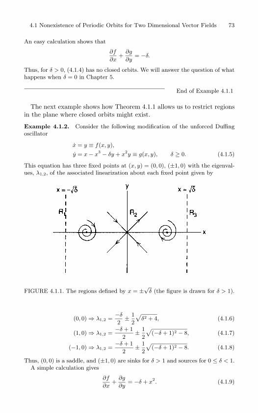
4.1 Nonexistence of Periodic Orbits for Two Dimensional Vector Fields 73
An easy calculation shows that
∂f
∂x+
∂g
∂y= −δ.
Thus, for δ > 0, (4.1.4) has no closed orbits. We will answer the question of what
happens when δ = 0 in Chapter 5.
End of Example 4.1.1
The next example shows how Theorem 4.1.1 allows us to restrict regionsin the plane where closed orbits might exist.
Example 4.1.2. Consider the following modification of the unforced Duffing
oscillator
x = y ≡ f(x, y),
y = x − x3 − δy + x2y ≡ g(x, y), δ ≥ 0. (4.1.5)
This equation has three fixed points at (x, y) = (0, 0), (±1, 0) with the eigenval-
ues, λ1,2, of the associated linearization about each fixed point given by
FIGURE 4.1.1. The regions defined by x = ±√δ (the figure is drawn for δ > 1).
(0, 0) ⇒ λ1,2 =−δ
2± 1
2
√δ2 + 4, (4.1.6)
(1, 0) ⇒ λ1,2 =−δ + 1
2± 1
2
√(−δ + 1)2 − 8, (4.1.7)
(−1, 0) ⇒ λ1,2 =−δ + 1
2± 1
2
√(−δ + 1)2 − 8. (4.1.8)
Thus, (0, 0) is a saddle, and (±1, 0) are sinks for δ > 1 and sources for 0 ≤ δ < 1.
A simple calculation gives
∂f
∂x+
∂g
∂y= −δ + x2. (4.1.9)
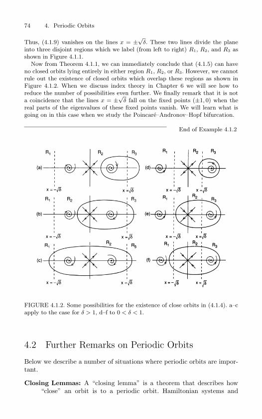
74 4. Periodic Orbits
Thus, (4.1.9) vanishes on the lines x = ±√δ. These two lines divide the plane
into three disjoint regions which we label (from left to right) R1, R2, and R3 as
shown in Figure 4.1.1.
Now from Theorem 4.1.1, we can immediately conclude that (4.1.5) can have
no closed orbits lying entirely in either region R1, R2, or R3. However, we cannot
rule out the existence of closed orbits which overlap these regions as shown in
Figure 4.1.2. When we discuss index theory in Chapter 6 we will see how to
reduce the number of possibilities even further. We finally remark that it is not
a coincidence that the lines x = ±√δ fall on the fixed points (±1, 0) when the
real parts of the eigenvalues of these fixed points vanish. We will learn what is
going on in this case when we study the Poincare–Andronov–Hopf bifurcation.
End of Example 4.1.2
FIGURE 4.1.2. Some possibilities for the existence of close orbits in (4.1.4). a–c
apply to the case for δ > 1, d–f to 0 < δ < 1.
4.2 Further Remarks on Periodic Orbits
Below we describe a number of situations where periodic orbits are impor-tant.
Closing Lemmas: A “closing lemma” is a theorem that describes how“close” an orbit is to a periodic orbit. Hamiltonian systems and
4.2 Further Remarks on Periodic Orbits 75
chaotic systems tend to possess periodic orbits in abundance, andit is often possible to characterize “most” orbits in terms of periodicorbits. 2 One of the first closing lemmas is due to Pugh [1967]. Robin-son [1978] provides an excellent introduction to the closing lemma.Recent references that describe the state of the art, as well as containreferences to the previous work are Mane [1982], Hayashi [1997], andAranson et al. [1997]. However, a word of caution is in order, Herman[1991] has constructed examples of Hamiltonian systems that con-tain no periodic orbits. Moreover, this situation is structurally stablein the sense that small perturbations of Herman’s examples also donot contain periodic orbits. This should be an indication of just howsubtle these questions may be.
Dynamical Averaging: It is often more meaningful to characterize sys-tems possessing complex dynamics through certain quantities involv-ing asymptotic time averages of trajectories. Examples of such quan-tities are power spectra, generalized dimensions, Liapunov exponents,and Kolmogorov entropy. Cvitanovic [1995] shows how under certainconditions such quantities can be calculated in terms of averages ofperiodic orbits.
Characterization of Chaos: Periodic orbits play a key role in under-standing the structure of chaotic attractors. See Lai et al. [1997],Zoldi and Greenside [1998], and the references in these papers.
Semiclassical Mechanics: Periodic orbits play an important role as abridge between classical and quantum mechanics. Unstable periodicorbits in classical systems may give rise to an extra, and unexpected,eigenstate density in their vicinity, which is referred to as a “scar”in the corresponding quantum mechanical system. See Kaplan andHeller [1999], and references therein.
Mathematical Biology: Periodic orbits are playing an increasingly im-portant role in the understanding of certain biological phenomena.See, e.g., So. et al. [1998], Lesher, et al. [1999], and the references inthese papers.
Time Series Analysis: Periodic orbits play a key role in distinguishingthe difference between complicated time series generated by deter-ministic chaos, versus those generated by random noise. See Carroll[1999], and references therein.
2Proving closing lemmas for specific classes of dynamical systems requiresprecise hypotheses and rather technical arguments. The quotation marks aroundthe words in this paragraph indicate that making these words mathematicallyprecise is very important.
76 4. Periodic Orbits
4.3 Exercises1. Show that the following vector field on the cylinder
v = −v,
θ = 1, (v, θ) ∈ R1 × S
1,
has a periodic orbit. Explain why Bendixson’s criterion does not hold.
2. Construct a vector field in R3 with negative divergence that possesses a periodic orbit.
Construct a vector field in R3 with negative divergence that contains a continuous
family of periodic orbits.
3. Prove Theorem 4.1.2.
4. The definition of periodic orbit for vector fields given in Definition 4.0.1 was givenfor the nonautonomous vector field (4.0.1). Suppose (4.0.1) is not periodic in time.That is, there is no constant T > 0 such that f(x, t) = f(x, t + T ) for all t, x in thedomain of definition. We refer to such nonautonomous vector fields as aperiodicallytime-dependent. Can aperiodically time dependent vector fields have periodic orbits?
5
Vector Fields Possessing anIntegral
For a general vector field
x = f(x), x ∈ Rn,
a scalar valued function I(x) is said to be an integral (sometimes the termfirst integral is used) if it is constant on trajectories, i.e.,
I(x) = ∇I(x) · x = ∇I(x) · f(x) = 0,
where “ · ” denotes the usual Euclidean inner product. From this relationwe see that the level sets of I(x) (which are generally (n− 1)-dimensional)are invariant sets. For two-dimensional vector fields the level sets actuallygive the trajectories of the system. We examine this case in more detail.
5.1 Vector Fields on Two-Manifolds Having anIntegral
In applications, three types of two-dimensional phase spaces occur fre-quently; they are (1) the plane, R
2 = R1 × R
1, (2) the cylinder, R1 × S1,
and (3) the two-torus, T 2 = S1 × S1. The vector field can be written as
x = f(x, y),y = g(x, y), (5.1.1)
where f and g are Cr (r ≥ 1), and as (x, y) ∈ R1 × R
1 for a vector fieldon the plane, as (x, y) ∈ R
1 × S1 for a vector field on the cylinder, and as(x, y) ∈ S1×S1 for a vector field on the torus, where S1 denotes the circle(which is sometimes referred to as a 1-torus, T 1). We now want to givesome examples of how these different phase spaces arise and at the sametime go into more detail concering the idea of an integrable vector field. Webegin with the unforced Duffing oscillator.
Example 5.1.1 (The Unforced Duffing Oscillator). We have been slowly dis-
covering the global structure of the phase space of the unforced Duffing oscillator
given by
x − x + δx + x3= 0, (5.1.2)
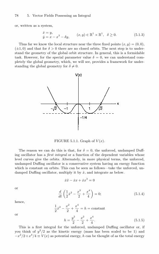
78 5. Vector Fields Possessing an Integral
or, written as a system,
x = y,y = x − x3 − δy,
(x, y) ∈ R1 × R
1, δ ≥ 0. (5.1.3)
Thus far we know the local structure near the three fixed points (x, y) = (0, 0),
(±1, 0) and that for δ > 0 there are no closed orbits. The next step is to under-
stand the geometry of the global orbit structure. In general, this is a formidable
task. However, for the special parameter value δ = 0, we can understand com-
pletely the global geometry, which, we will see, provides a framework for under-
standing the global geometry for δ = 0.
FIGURE 5.1.1. Graph of V (x).
The reason we can do this is that, for δ = 0, the unforced, undamped Duff-
ing oscillator has a first integral or a function of the dependent variables whose
level curves give the orbits. Alternately, in more physical terms, the unforced,
undamped Duffing oscillator is a conservative system having an energy function
which is constant on orbits. This can be seen as follows—take the unforced, un-
damped Duffing oscillator, multiply it by x, and integrate as below.
xx − xx + xx3= 0
ord
dt
(1
2x2 − x2
2+
x4
4
)= 0; (5.1.4)
hence,
1
2x2 − x2
2+
x4
4= h = constant
or
h =y2
2− x2
2+
x4
4. (5.1.5)
This is a first integral for the unforced, undamped Duffing oscillator or, if
you think of y2/2 as the kinetic energy (mass has been scaled to be 1) and
−x2/2+x4/4 ≡ V (x) as potential energy, h can be thought of as the total energy
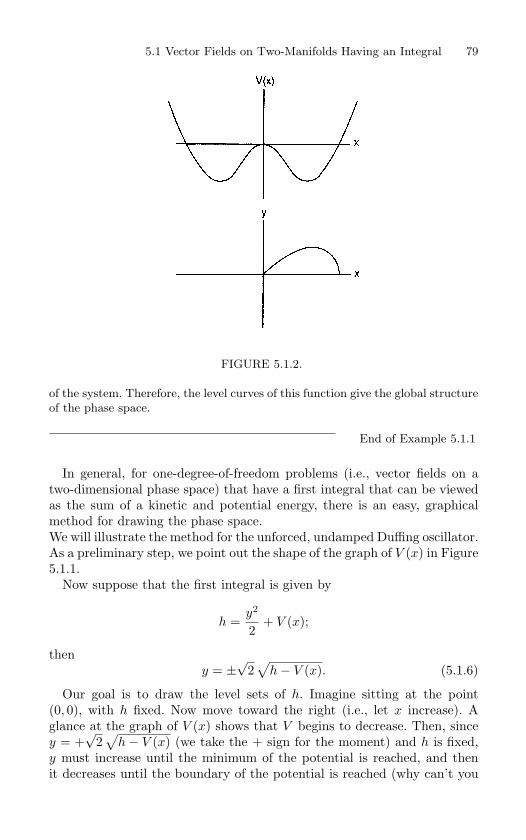
5.1 Vector Fields on Two-Manifolds Having an Integral 79
FIGURE 5.1.2.
of the system. Therefore, the level curves of this function give the global structure
of the phase space.
End of Example 5.1.1
In general, for one-degree-of-freedom problems (i.e., vector fields on atwo-dimensional phase space) that have a first integral that can be viewedas the sum of a kinetic and potential energy, there is an easy, graphicalmethod for drawing the phase space.We will illustrate the method for the unforced, undamped Duffing oscillator.As a preliminary step, we point out the shape of the graph of V (x) in Figure5.1.1.
Now suppose that the first integral is given by
h =y2
2+ V (x);
theny = ±
√2√
h− V (x). (5.1.6)
Our goal is to draw the level sets of h. Imagine sitting at the point(0, 0), with h fixed. Now move toward the right (i.e., let x increase). Aglance at the graph of V (x) shows that V begins to decrease. Then, sincey = +
√2√
h− V (x) (we take the + sign for the moment) and h is fixed,y must increase until the minimum of the potential is reached, and thenit decreases until the boundary of the potential is reached (why can’t you
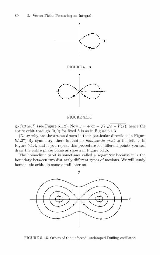
80 5. Vector Fields Possessing an Integral
FIGURE 5.1.3.
FIGURE 5.1.4.
go farther?) (see Figure 5.1.2). Now y = + or −√
2√
h− V (x); hence theentire orbit through (0, 0) for fixed h is as in Figure 5.1.3.
(Note: why are the arrows drawn in their particular directions in Figure5.1.3?) By symmetry, there is another homoclinic orbit to the left as inFigure 5.1.4, and if you repeat this procedure for different points you candraw the entire phase plane as shown in Figure 5.1.5.
The homoclinic orbit is sometimes called a separatrix because it is theboundary between two distinctly different types of motions. We will studyhomoclinic orbits in some detail later on.
FIGURE 5.1.5. Orbits of the unforced, undamped Duffing oscillator.
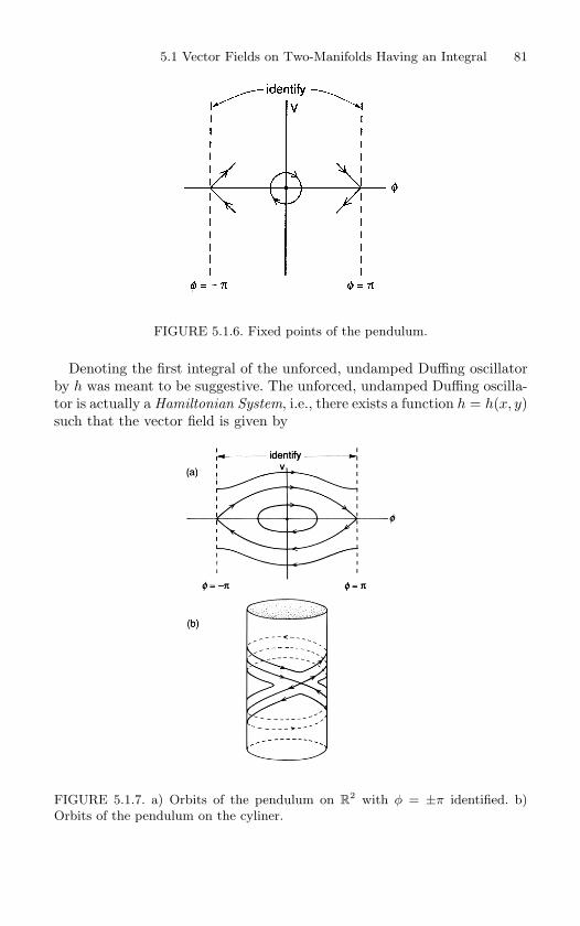
5.1 Vector Fields on Two-Manifolds Having an Integral 81
FIGURE 5.1.6. Fixed points of the pendulum.
Denoting the first integral of the unforced, undamped Duffing oscillatorby h was meant to be suggestive. The unforced, undamped Duffing oscilla-tor is actually a Hamiltonian System, i.e., there exists a function h = h(x, y)such that the vector field is given by
FIGURE 5.1.7. a) Orbits of the pendulum on R2 with φ = ±π identified. b)
Orbits of the pendulum on the cyliner.
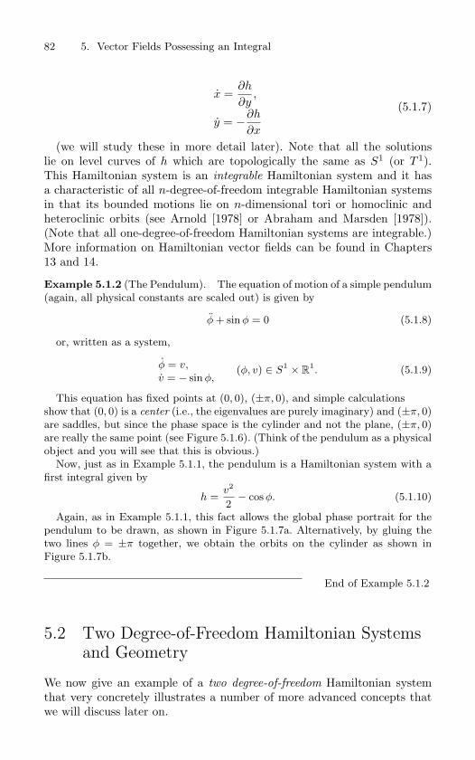
82 5. Vector Fields Possessing an Integral
x =∂h
∂y,
y = −∂h
∂x
(5.1.7)
(we will study these in more detail later). Note that all the solutionslie on level curves of h which are topologically the same as S1 (or T 1).This Hamiltonian system is an integrable Hamiltonian system and it hasa characteristic of all n-degree-of-freedom integrable Hamiltonian systemsin that its bounded motions lie on n-dimensional tori or homoclinic andheteroclinic orbits (see Arnold [1978] or Abraham and Marsden [1978]).(Note that all one-degree-of-freedom Hamiltonian systems are integrable.)More information on Hamiltonian vector fields can be found in Chapters13 and 14.
Example 5.1.2 (The Pendulum). The equation of motion of a simple pendulum
(again, all physical constants are scaled out) is given by
φ + sin φ = 0 (5.1.8)
or, written as a system,
φ = v,v = − sin φ,
(φ, v) ∈ S1 × R1. (5.1.9)
This equation has fixed points at (0, 0), (±π, 0), and simple calculations
show that (0, 0) is a center (i.e., the eigenvalues are purely imaginary) and (±π, 0)
are saddles, but since the phase space is the cylinder and not the plane, (±π, 0)
are really the same point (see Figure 5.1.6). (Think of the pendulum as a physical
object and you will see that this is obvious.)
Now, just as in Example 5.1.1, the pendulum is a Hamiltonian system with a
first integral given by
h =v2
2− cos φ. (5.1.10)
Again, as in Example 5.1.1, this fact allows the global phase portrait for the
pendulum to be drawn, as shown in Figure 5.1.7a. Alternatively, by gluing the
two lines φ = ±π together, we obtain the orbits on the cylinder as shown in
Figure 5.1.7b.
End of Example 5.1.2
5.2 Two Degree-of-Freedom Hamiltonian Systemsand Geometry
We now give an example of a two degree-of-freedom Hamiltonian systemthat very concretely illustrates a number of more advanced concepts thatwe will discuss later on.
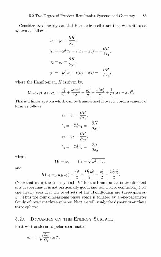
5.2 Two Degree-of-Freedom Hamiltonian Systems and Geometry 83
Consider two linearly coupled Harmonic oscillators that we write as asystem as follows
x1 = y1 =∂H
∂y1,
y1 = −ω2x1 − c(x1 − x2) = − ∂H
∂x1,
x2 = y2 =∂H
∂y2,
y2 = −ω2x2 − c(x2 − x1) = − ∂H
∂x2,
where the Hamiltonian, H is given by,
H(x1, y1, x2, y2) =y21
2+
ω2x21
2+
y22
2+
ω2x22
2+
12c(x1 − x2)2.
This is a linear system which can be transformed into real Jordan canonicalform as follows
u1 = v1 =∂H
∂v1,
v1 = −Ω21u1 = − ∂H
∂u1,
u2 = v2 =∂H
∂v2,
v2 = −Ω22u2 = − ∂H
∂u2,
whereΩ1 = ω, Ω2 =
√ω2 + 2c,
and
H(u1, v1, u2, v2) =v21
2+
Ω21u
21
2+
v22
2+
Ω22u
22
2.
(Note that using the same symbol “H” for the Hamiltonian in two differentsets of coordinates is not particularly good, and can lead to confusion.) Nowone clearly sees that the level sets of the Hamiltonian are three-spheres,S3. Thus the four dimensional phase space is foliated by a one-parameterfamily of invariant three-spheres. Next we will study the dynamics on thesethree-spheres.
5.2a Dynamics on the Energy SurfaceFirst we transform to polar coordinates
ui =√
2Ii
Ωisin θi,
84 5. Vector Fields Possessing an Integral
=⇒ ui =√
12IiΩi
Ii sin θi +√
2Ii
Ωiθi cos θi =
√2IiΩi cos θi,
vi =√
2IiΩi cos θi,
=⇒ vi =√
Ωi
2IiIi cos θi −
√2IiΩiθi sin θi = Ω2
i
√2Ii
Ωisin θi,
i = 1, 2.
Combining these relations with the equations of motion in the u1 − v1 −u2 − v2 coordinates gives
Ii = 0θi = Ωi, i = 1, 2.
Full Equations of Motion
The full equations of motion are given as
θ1 = Ω1 = ∂H∂I1
,
I1 = 0 = − ∂H∂θ1
,
θ2 = Ω2 = ∂H∂I2
,
I2 = 0 = − ∂H∂θ2
,
with HamiltonianH(I1, I2) = I1Ω1 + I2Ω2.
Equations of Motion Restricted to the Energy Surface
Since trajectories are restricted to lie in the three dimensional energy sur-face the dynamics is really three dimensional. Now we show how this canbe realized in the equations of motion.
The equation for the energy surface is
H(I1, I2) = I1Ω1 + I2Ω2 = h = constant,
which we can easily rearrange and explicitly exhibit I2 as a function of I1and h
I2 =h− I1Ω1
Ω2= I2(I1, h).
Hence, if we know I1 and h, we know I2. Therefore, on the energy surface,the equations reduce to
θ1 = Ω1,
θ2 = Ω2,
I1 = 0. (5.2.1)
5.3 Exercises 85
From these equations we see that the energy surface is foliated by a one-parameter family of invariant two-tori.
5.2b Dynamics on an Individual TorusFixing h and I1 chooses an individual two-torus. The trajectories on thistorus are given by
θ1(t) = Ω1t + Ω10,θ2(t) = Ω2t + Ω20.
The nature of the trajectories depend on the number Ω1Ω2
. If this is a ratio-nal number then all trajectories are periodic. If it is irrational, then anytrajectory densely covers the torus. These statements are proved in Section10.4a.
For a more detailed study of the geometry of two coupled linear oscilla-tors, which makes connections with many deeper topics such as the Hopffibration of the three-sphere and knots, see the excellent paper of Meyer[1990].
5.3 Exercises1. Consider the following vector fields.
a) x + µx = 0, x ∈ R1.
b) x + µx + x2 = 0, x ∈ R1.
c) x + µx + x3 = 0, x ∈ R1.
d)x = −µy + xy,y = µx + 1
2 (x2 − y2), (x, y) ∈ R2.
i) Write a), b) and c) as systems.ii) Find and determine the nature of the stability of the fixed points.iii) Find the first integrals and draw all phase curves for µ < 0, µ = 0, and
µ > 0.
2. Euler’s equations of motion for a free rigid body are
mi = Iiωi, i = 1, 2, 3, I1 > I2 > I3
m1 =I2 − I3
I2I3m2m3,
m2 =I3 − I1
I1I3m1m3, (m1, m2, m3) ∈ R
3,
m3 =I1 − I2
I1I2m1m2,
a) Find and determine the nature of the stability of the fixed points.b) Show that the functions
H(m1, m2, m3) =12
[m2
1
I1+
m22
I2+
m23
I3
],
L(m1, m2, m3) = m21 + m
22 + m
23
are constants on orbits.
86 5. Vector Fields Possessing an Integral
c) For fixed L, draw all phase curves.
3. At the beginning of this chapter we defined the notion of an integral for autonomousvector fields. An integral is a (scalar valued) function that is constant on trajectories,or more geometrically, it is a function having the property that the vector field istangent to its level sets. Generalize these ideas for the case of nonautonomous vectorfields.
4. Consider the a map:x → g(x), x ∈ R
n,
orxn+1 = g(xn).
Define the notion of an integral for maps.
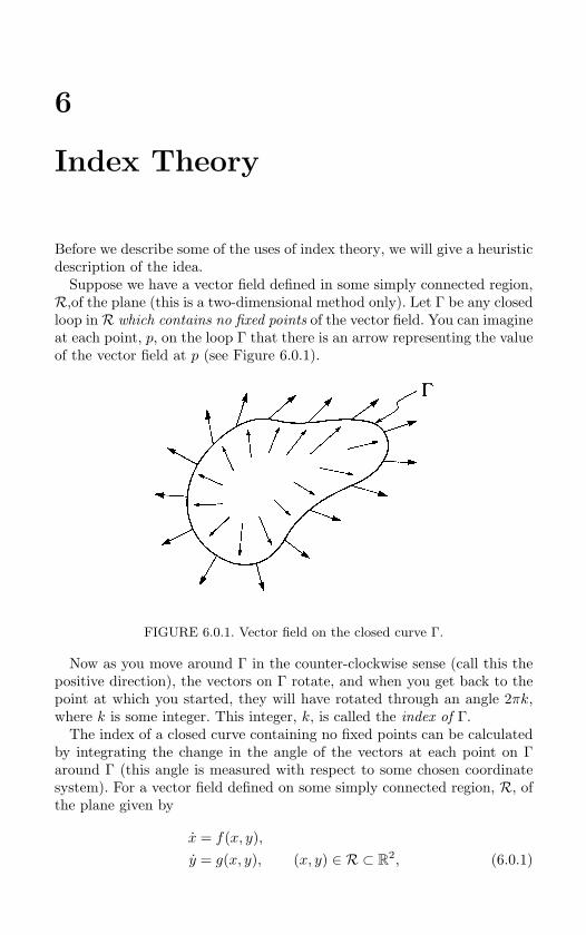
6
Index Theory
Before we describe some of the uses of index theory, we will give a heuristicdescription of the idea.
Suppose we have a vector field defined in some simply connected region,R,of the plane (this is a two-dimensional method only). Let Γ be any closedloop inR which contains no fixed points of the vector field. You can imagineat each point, p, on the loop Γ that there is an arrow representing the valueof the vector field at p (see Figure 6.0.1).
FIGURE 6.0.1. Vector field on the closed curve Γ.
Now as you move around Γ in the counter-clockwise sense (call this thepositive direction), the vectors on Γ rotate, and when you get back to thepoint at which you started, they will have rotated through an angle 2πk,where k is some integer. This integer, k, is called the index of Γ.
The index of a closed curve containing no fixed points can be calculatedby integrating the change in the angle of the vectors at each point on Γaround Γ (this angle is measured with respect to some chosen coordinatesystem). For a vector field defined on some simply connected region, R, ofthe plane given by
x = f(x, y),y = g(x, y), (x, y) ∈ R ⊂ R
2, (6.0.1)
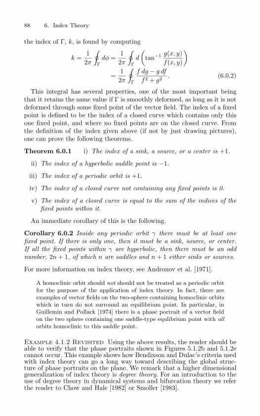
88 6. Index Theory
the index of Γ, k, is found by computing
k =12π
∮Γ
dφ =12π
∮Γ
d
(tan−1 g(x, y)
f(x, y)
)
=12π
∮Γ
f dg − g df
f2 + g2 . (6.0.2)
This integral has several properties, one of the most important beingthat it retains the same value if Γ is smoothly deformed, as long as it is notdeformed through some fixed point of the vector field. The index of a fixedpoint is defined to be the index of a closed curve which contains only thisone fixed point, and where no fixed points are on the closed curve. Fromthe definition of the index given above (if not by just drawing pictures),one can prove the following theorems.
Theorem 6.0.1 i) The index of a sink, a source, or a center is +1.
ii) The index of a hyperbolic saddle point is −1.
iii) The index of a periodic orbit is +1.
iv) The index of a closed curve not containing any fixed points is 0.
v) The index of a closed curve is equal to the sum of the indices of the
fixed points within it.
An immediate corollary of this is the following.
Corollary 6.0.2 Inside any periodic orbit γ there must be at least one
fixed point. If there is only one, then it must be a sink, source, or center.
If all the fixed points within γ are hyperbolic, then there must be an odd
number, 2n + 1, of which n are saddles and n + 1 either sinks or sources.
For more information on index theory, see Andronov et al. [1971].
A homoclinic orbit should not should not be treated as a periodic orbit
for the purpose of the application of index theory. In fact, there are
examples of vector fields on the two-sphere containing homoclinic orbits
which in turn do not surround an equilibrium point. In particular, in
Guillemin and Pollack [1974] there is a phase portrait of a vector field
on the two sphere containing one saddle-type equlibrium point with allorbits homoclinic to this saddle point.
Example 4.1.2 Revisited Using the above results, the reader should beable to verify that the phase portraits shown in Figures 5.1.2b and 5.1.2ecannot occur. This example shows how Bendixson and Dulac’s criteria usedwith index theory can go a long way toward describing the global struc-ture of phase portraits on the plane. We remark that a higher dimensionalgeneralization of index theory is degree theory. For an introduction to theuse of degree theory in dynamical systems and bifurcation theory we referthe reader to Chow and Hale [1982] or Smoller [1983].
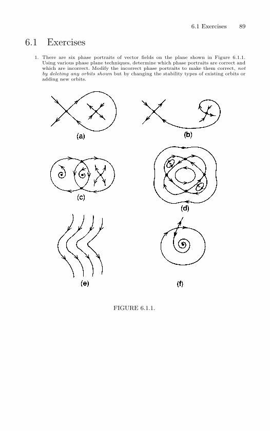
6.1 Exercises 89
6.1 Exercises1. There are six phase portraits of vector fields on the plane shown in Figure 6.1.1.
Using various phase plane techniques, determine which phase portraits are correct andwhich are incorrect. Modify the incorrect phase portraits to make them correct, notby deleting any orbits shown but by changing the stability types of existing orbits oradding new orbits.
FIGURE 6.1.1.
7
Some General Properties ofVector Fields: Existence,Uniqueness, Differentiability,and Flows
In this section we want to give some of the basic theorems describing generalproperties of solutions of vector fields. Since it is just as easy to treat thenonautonomous case we will do so.
Consider the vector field
x = f(x, t), (7.0.1)
where f(x, t) is Cr, r ≥ 1, on some open set U ⊂ Rn × R
1.
7.1 Existence, Uniqueness, Differentiability withRespect to Initial Conditions
Theorem 7.1.1 Let (x0, t0) ∈ U . Then there exists a solution of (7.0.1)
through the point x0 at t = t0, denoted x(t, t0, x0) with x(t0, t0, x0) = x0, for
|t−t0| sufficiently small. This solution is unique in the sense that any other
solution of (7.0.1) through x0 at t = t0 must be the same as x(t, t0, x0) on
their common interval of existence. Moreover, x(t, t0, x0) is a Cr function
of t, t0, and x0.
Proof: See Arnold [1973], Hirsch and Smale [1974], or Hale [1980].
We remark that it is possible to weaken the assumptions on f(x, t) andstill obtain existence and uniqueness. We refer the reader to Hale [1980] fora discussion.
Theorem 7.1.1 only guarantees existence and uniqueness for sufficientlysmall time intervals. The following result allows us to uniquely extend thetime interval of existence.
7.2 Continuation of Solutions 91
7.2 Continuation of Solutions
Let C ⊂ U ⊂ Rn × R
1 be a compact set containing (x0, t0).
Theorem 7.2.1 The solution x(t, t0, x0) can be uniquely extended back-
ward and forward in t up to the boundary of C.
Proof: See Hale [1980].
Theorem 7.2.1 tells us how solutions fail to exist; namely, they “blowup.” Consider the following example.
Example 7.2.1. Consider the equation
x = x2, x ∈ R1. (7.2.1)
The solution of (7.2.1) through x0 at t = 0 is given by
x(t, 0, x0) =−x0
x0t − 1. (7.2.2)
It should be clear that (7.2.2) does not exist for all time, since it becomes infinite
at t = 1/x0. This example also shows that the time interval of existence may
depend on x0.
End of Example 7.2.1
In practice we often encounter vector fields depending on parameters,and it is often necessary to differentiate the solutions with respect to theparameters. The following result covers this situation.
7.3 Differentiability with Respect to Parameters
Consider the vector fieldx = f(x, t;µ), (7.3.1)
where f(x, t;µ) is Cr (r ≥ 1) on some open set U ⊂ Rn × R
1 × Rp.
Theorem 7.3.1 For (t0, x0, µ) ∈ U the solution x(t, t0, x0, µ) is a Cr func-
tion of t, t0, x0, and µ.
Proof: See Arnold [1973] or Hale [1980].
At this stage we would like to point out some special properties of Cr,r ≥ 1, autonomous vector fields which will prove useful.
92 7. General Properties of Vector Fields
7.4 Autonomous Vector Fields
Consider the vector field
x = f(x), x ∈ Rn, (7.4.1)
where f(x) is Cr, r ≥ 1, on some open set U ∈ Rn. For simplicity, let us
suppose that the solutions exist for all time (we leave it as an exercise tomake the necessary modifications when solutions exist only on finite timeintervals). The following three results are very useful in applications.
Proposition 7.4.1 If x(t) is a solution of (7.4.1), then so is x(t + τ) for
any τ ∈ R.
Proof: By definitiondx(t)
dt= f
(x(t)
). (7.4.2)
Hence, we have
dx(t + τ)dt
∣∣∣∣t=t0
=dx(t)
dt
∣∣∣∣t=t0+τ
= f(x(t0 + τ)
)= f
(x(t + τ)
)∣∣t=t0
ordx(t + τ)
dt
∣∣∣∣t=t0
= f(x(t + τ)
)∣∣t=t0
. (7.4.3)
Since (7.4.3) is true for any t0 ∈ R, the result follows.
Note that Proposition 7.4.1 does not hold for nonautonomous vectorfields. Consider the following example.
Example 7.4.1. Consider the nonautonomous vector field
x = et, x ∈ R1. (7.4.4)
The solution of (7.4.4) is given by
x(t) = et, (7.4.5)
and it should be clear that
x(t + τ) = et+τ(7.4.6)
is not a solution of (7.4.4) for τ = 0.
End of Example 7.4.1
The following proposition lies at the heart of the Poincare-Bendixsontheorem.
7.4 Autonomous Vector Fields 93
Proposition 7.4.2 For any x0 ∈ Rn there exists only one solution of
(7.4.1) passing through this point.
Proof: We will show that if this proposition weren’t true, then uniquenessof solutions would be violated.
Let x1(t), x2(t) be solutions of (7.4.1) satisfying
x1(t1) = x0,
x2(t2) = x0.
By Proposition 7.4.1
x2(t) ≡ x2(t− (t1 − t2)
)is also a solution of (7.4.1) satisfying
x2(t1) = x0.
Hence, by Theorem 7.1.1, x1(t) and x2(t) must be identical.
Since for autonomous vector fields time-translated solutions remain so-lutions (i.e., Proposition 7.4.1 holds), it suffices to choose a fixed initialtime, say t0 = 0, which is understood and therefore often omitted from thenotation (as we do now).
Proposition 7.4.3 (Properties of a Flow)
i) x(t, x0) is Cr.
ii) x(0, x0) = x0.
iii) x(t + s, x0) = x(t, x(s, x0)
).
Proof: i) follows from Theorem 7.1.1, ii) is by definition, and iii) followsfrom Proposition 7.4.2; namely, x(t, x0) ≡ x(t + s, x0) and x
(t, x(s, x0)
)are both solutions of (7.4.1) satisfying the same initial conditions at t = 0.Hence, by uniqueness, they must coincide.
Proposition 7.4.3 shows that the solutions of (7.4.1) form a one-parameterfamily of Cr, r ≥ 1, diffeomorphisms of the phase space (invertibility comesfrom iii)). This is referred to as a phase flow or just a flow. A commonnotation for flows is φ(t, x) or φt(x).
Let us comment a bit more on this notation φt(x). The part of Theorem7.1.1 dealing with differentiability of solutions with respect to x0 (regardingt and t0 as fixed) allows us to think differently about the solutions ofordinary differential equations. More precisely, in the solution x(t, t0, x0),we can think of t and t0 as fixed and then study how the map x(t, t0, x0)moves sets of points around in phase space. This is the global, geometrical
94 7. General Properties of Vector Fields
view of the study of dynamical systems. For a set U ⊂ Rn, we would denote
its image under this map by x(t, t0, U). Since points in phase space are alsolabeled by the letter x, it is often less confusing to change the notation forthe solutions, which is why we use the symbol φ. This point of view willbecome more apparent when we study the construction of Poincare maps.
Finally, let us note that in the study of ordinary differential equations onemight believe the problem to be finished when the “solution” x(t, t0, x0) isfound. The rest of the book will show that this is not the case, but, on thecontrary, that this is when the story begins to get really interesting.
7.5 Nonautonomous Vector Fields
It should be clear that Propositions 7.4.1, 7.4.2, and 7.4.3 do not holdfor nonautonomous vector fields. However, we can always make a nonau-tonomous vector field autonomous by redefining time as a new dependentvariable. This is done as follows.
By writing (7.0.1) asdx
dt=
f(x, t)1
(7.5.1)
and using the chain rule, we can introduce a new independent variable sso that (7.5.1) becomes
dx
ds≡ x′ = f(x, t),
dt
ds≡ t′ = 1.
(7.5.2)
If we define y = (x, t) and g(y) = (f(x, t), 1), we see that (7.5.2) becomes
y′ = g(y), y ∈ Rn × R
1. (7.5.3)
Of course, knowledge of the solutions of (7.5.3) implies knowledge of thesolutions of (7.0.1) and vice versa. For example, if x(t) is a solution of(7.0.1) passing through x0 at t = t0, i.e., x(t0) = x0, then y(s) = (x(s+ t0),t(s) = s + t0) is a solution of (7.5.3) passing through y0 ≡
(x(t0), t0
)at
s = 0.Every vector field can thus be viewed as an autonomous vector field.
This apparently trivial trick is a great conceptual aid in the constructionof Poincare maps for time-periodic and quasiperiodic vector fields, as weshall see in Chapter 10. Notice, however, that in redefining time as a de-
pendent variable, it may then be introduced in various situations requiringspecification of initial positions (i.e., specifying x0); in particular, the readershould reexamine the definition of stability given in Chapter 1. There arealternative, and more useful, views of nonautonomous vector fields that
7.5 Nonautonomous Vector Fields 95
we briefly describe since they are becoming more and more prominent incurrent developments in dynamical systems theory.
Let x(t, t0, x0), denote a solution of (7.0.1) with x(t0, t0, x0) = x0. Thenthe analog of property iii) of Proposition 7.4.3 is the following:
x(t2, t0, x0) = x(t2, t1, x(t1, t0, x0)), ∀x0 ∈ Rn, and all t0 ≤ t1 ≤ t2,
(7.5.4)which is called the cocycle property. The notion of a cocycle is centralto current developments in ergodic theory (Katok and Hasselblatt [1995]),random dynamical systems (Arnold [1998]), and nonautonomous dynamicalsystems (Kloeden and Schmalfuss [1997]). We will describe the cocycleformalism in more generality, but we first describe the skew-product flowapproach to nonautonomous vector fields.
7.5a The Skew-Product Flow ApproachThe skew-product flow approach is a way of dealing with nonautonomousvector fields so as to retain the flow properties as described in Proposition7.4.1. This approach has been pioneered by Sell [1967a, b], [1971].
The crucial observation leading to the development of the approach is thefollowing. Suppose x(t) is a solution of x = f(x, t). Then xτ (t) ≡ x(t + τ)is a solution of xτ (t) = fτ (xτ (t), t) ≡ f(x(t + τ), t + τ) (compare this withthe proof of Proposition 7.4.1).
We first define the space of nonautonomous vector fields whose timetranslates remain within the space, i.e.,
F ≡ Space of functions f : Rn × R → R
n such thatfτ (·, ·) ≡ f(·, ·+ τ) ∈ F for all τ ∈ R.
We then define the group of shift operators on F :
θτ : F → F ,
f → θτf ≡ fτ , ∀τ ∈ R, (7.5.5)
and we define the product space:
X ≡ Rn ×F .
A slight variation in notation is now useful. Let x(t, x0, f) denote a solu-tion of x = f(x, t) with x(0, x0, f) = x0. Finally, we define the family ofmappings:
Ψt : X → X ,
(x0, f) → (x(t, x0, f), θtf) . (7.5.6)
96 7. General Properties of Vector Fields
Ψt is a one-parameter family of mappings of X into X , or flow 1. Thisfollows easily from the fact that the identity (i.e., the analog of (7.5.4)):
x(t + s, x0, f) = x(t, x(s, x0, f), θsf), (7.5.7)
is the same asΨt+s(x0, f) = Ψt Ψs(x0, f). (7.5.8)
It is easy to see that the role of the shift operators θτ is to advance theexplicit time argument in the vector field. The reader should imagine thisin the context of attempting to prove Proposition 7.4.1 for nonautonomousvector fields.
The notion of a skew-product flow derived from nonautonomous vectorfields can be made general, and is referred to as a skew-product dynami-
cal system (or just skew dynamical system). This is done as follows. LetM denote an n-dimensional manifold and S a metric space (or, possibly,something more general). Consider a map of the form:
f : M × S →M × S,
(m, s) → (φ(m, s), σ(s)) . (7.5.9)
Further, we will assume that for each fixed s, the map φ(·, s) : M → M isa Cr diffeomorphism. Then the system defined by (7.5.9) is referred to asa skew dynamical system over the base σ : S → S.
Skew dynamical systems play a central role in dynamical systems in theirown right. The following topics and references are representative of theseareas and applications.
General Theory of Skew-Product Dynamical Systems: Sacker andSell [1977], Sacker [1976], Shen and Yi [1998] develop many basicproperties of skew-product dynamical systems.
Invariant Manifold Theorems: Chow and Yi [1994], Yi [1993a, b] proveinvariant manifold theorems for nonautonomous vector fields by usingthe skew-product dynamical systems approach.
Global Stability: Meyer and Zhang [1996] develop many of the basic con-cepts of skew-product dynamical systems (e.g., stable and unstablemanifolds of hyperbolic trajectories, hyperbolic sets, shadowing, basicsets, etc. ) for studying global dynamics in much the same manner asdescribed in, e.g. Shub [1987], for standard differential dynamical dy-namical systems, i.e., dynamics defined by iterated diffeomorphismsor flows on manifolds. Johnson and Kloeden [2001] discuss attractorsfor skew-product dynamical systems.
1It is important (but not for our descriptive purposes here) to have a topologyon X such that the map (t, x0, f) → x(t, x0, f) is continuous, see Sell [1967a, b]for details.
7.5 Nonautonomous Vector Fields 97
7.5b The Cocycle ApproachThe cocycle property can be expressed in a general formalism. Let P denotea parameter space. In different applications P could be a compact metricspace, a function space, or a probability space. Let Θ = θt | t ∈ R denotea one-parameter family of mappings of P into itself, i.e.,
θt : P → P,
p → θtp,
withθt θs = θt+s, ∀t, s ∈ R,
andθ0 = id.
Then we have the following definition.
Definition 7.5.1 (Cocycle on Rn) A family of mappings
φt,p : Rn → R
n, t ∈ R, p ∈ P,
is called a cocycle on Rn with respect to a group Θ of mappings on P if:
1. φ0,p = id,
2. φt+s,p = φt,θsp φs,p,
for all t, s ∈ R, p ∈ P .
The reader should be able to verify that (7.5.7) is an example of a cocycle.We show that the cocycle relation for nonautonomous vector fields given
in (7.5.4) can be interpreted in terms of this general formalism. This canbe seen as follows. Let P = R, θtt0 = t0 + t and t0 ≤ t0 + s ≤ t0 + s + t.Then we have:
φt+s,p = x(t0+s+t, t0, x0) = x(t0+s+t, t0+s, x(t0+s, t0, x0)) = φt,θspφs,p.
7.5c Dynamics Generated by a Bi-InfiniteSequence of Maps
There is yet another way to study the dynamics of nonautonomous vectorfields. The dynamical systems point of view has taught us that it is oftenfruitful to study the trajectories of (7.0.1) by passing to an n-dimensionaldiscrete time system, or map. We will explore this in some detail when weconsider Poincare maps in Chapter 10. In this setting the dynamical aspectsof geometrical structures in phase space often appear more simple than inthe continuous time setting. One reason for this is that the trajectoriesof time-dependent velocity fields may intersect themselves. The resulting
98 7. General Properties of Vector Fields
trajectory can appear very complicated, but when “sampled” at discretetime its discrete time analog may appear more simple, and any underlyinggeometrical structure may be more apparent.
There are a variety of ways of constructing a discrete time map from thetrajectories of (7.0.1). However, the overriding issue is that the dynamicsof the resulting discrete time system should somehow correlate with thedynamics of the continuous time system. The most straightforward way inwhich this connection can be made is if the trajectory of the velocity fieldinterpolates the discrete set of points corresponding to the trajectory of thediscrete time system.
With this in mind, we define the following n-dimensional map from tra-jectories of (7.0.1) as follows:
fn(x0) ≡ x (t0 + nT, t0 + (n− 1)T, x0) , (7.5.10)
where T > 0 is some fixed time increment and n ∈ ZZ. We want to describethe evolution of x0 in the vector field (7.0.1) in terms of the map (7.5.10).Unfortunately, this cannot be done in the case when the velocity field hasan arbitrary time-dependence since generally
fj(x0) = fk(x0) j = k.
Instead, we must use the bi-infinite sequence of maps
fn(·) , n ∈ ZZ,
since the orbit of a point x0 in the vector field (7.0.1), i.e.,
x ∈ Rn |x = x(t, t0, x0), t ∈ R ,
interpolates the following bi-infinite sequence of points.
. . . , f−n f−n+1 · · · f−1(x0), . . . , f−1(x0), x0, f1(x0),. . . , fn fn−1 · · · f1(x0), . . . .
We remark that in the usual situation studied in dynamical systems the-ory, if the velocity field is time periodic, with period T , then fj(·) =fk(·), ∀j, k ∈ ZZ. Some basic results for dynamics generated by sequencesof maps (such as a stable and unstable manifold theorem) can be foundin Katok and Hasselblatt [1995]; see also de Blasi and Schinas [1973] andIrwin [1973].
For the most part in this book we will be considering autonomous vec-tor fields or maps constructed from nonautonomous vector fields (morespecifically, maps constructed from time-periodic and quasiperiodic vectorfields). Consequently, henceforth we will state definitions in the context ofautonomous vector fields and maps.
7.6 Liouville’s Theorem 99
7.6 Liouville’s Theorem
Now we prove several results due to Liouville which describe the time evo-lution of volumes under a flow.
Consider a general autonomous vector field
x = f(x), x ∈ Rn,
and suppose that it generates a flow φt(·). Let D0 denote a domain in Rn
and let Dt ≡ φt(D0) denote the evolution of D0 under the flow. Let V (t)denote the volume of Dt. Then we have the following lemma.
Lemma 7.6.1
dV
dt
∣∣∣∣t=0
=∫
D0
∇ · fdx,
where ∇ · f = ∂f1∂x1
+ · · ·+ ∂fn
∂xndenotes the divergence of a vector field.
Proof: From the definition of the Jacobian of a transformation we have
V (t) =∫
D0
det∂φt(x)
∂xdx. (7.6.1)
By Taylor expanding the flow in t:
φt(x) = x + f(x)t +O(t2),
it follows that∂φt(x)
∂x= id +
∂f
∂xt +O(t2),
where “id” denotes the n × n identity matrix. Using this relation, and astandard result from linear algebra on the expansion of the determinant(see, e.g., Arnold [1973], Sec. 16.3), we obtain
det∂φt(x)
∂x= det
(id +
∂f
∂xt
)+O(t2),
= 1 + tr(
∂f
∂x
)t +O(t2).
Substituting this expression into (7.6.1) gives
V (t) = V (0) +∫
D0
t∇ · fdx +O(t2),
from which the lemma follows immediately.
100 7. General Properties of Vector Fields
Now there is nothing distinguished about the point t = 0. In particular,Lemma 7.6.1 can be written in the form
dV
dt
∣∣∣∣t=t0
=∫
Dt0
∇ · fdy, (7.6.2)
for an arbitrary t0 = 0. This can be seen as follows. Let
y = φt0(x),
for some arbirary t0 = 0. Then
V (t) =∫
Dt0
det∂φt(y)
∂ydy.
Nowφt(y) = y + f(y)t +O(t2),
and∂φt(y)
∂y= id +
∂f
∂yt +O(t2).
Using these three formulas we can repeat exactly the same steps as in theproof of Lemma 7.6.1 to conclude that (7.6.2) holds.
We can use these results to derive equations for the time evolution ofvolumes which can be explicitly solved in certain cases.
Suppose that the divergence is everywhere constant, i.e.,
∇ · f = c = constant.
Using (7.6.2), since t0 is arbitrary the evolution equation for the volume isgiven by
V = cV,
which has the obvious solution
V (t) = ectV (0). (7.6.3)
In the case where the vector field is divergence free (i.e., c = 0), we havethe following result that is typically referred to as Liouville’s Theorem.
Theorem 7.6.2 (Liouville) Suppose ∇ · f = 0. Then for any region D0,
V (t) = V (0),
where V (0) is the volume of D0 and V (t) is the volume of φt (D0).
Proof: This follows immediately from (7.6.3) by setting c = 0.
7.7 Exercises 101
7.6a Volume Preserving Vector Fields and thePoincare Recurrence Theorem
We refer to vector fields which have zero divergence as divergence free orvolume preserving vector fields.
Volume preserving dynamical systems, which we think of as flows gener-ated by divergence free vector fields or volume preserving maps, may havea certain recurrence property that is attributed to Poincare. We now provethis Poincare recurrence theorem.
Theorem 7.6.3 (Poincare Recurrence Theorem) Suppose g : Rn →
Rn is a continuous, one-to-one mapping, and suppose that D ⊂ R
n is a
compact invariant set, i.e., g(D) = D. Let x be any point in D and let
U be any neighborhood of x. Then there exists a point x ∈ U such that
gn(x) ∈ U for some n > 0.
Proof: Consider the sets defined by the images of U under iteration by g:
U, g(U), g2(U), . . . , gn(U), . . . .
Since g is volume-preserving, each of these has the same volume. If theynever intersected, then D would have infinite volume. But D is compact,therefore there must exist integers k ≥ 0, l ≥ 0, with k > l, such that
gk(U) ∩ gl(U) = ∅.
Thereforegk−l(U) ∩ U = ∅.
If we let y = gk−l(x), then x ∈ U and gn(x) ∈ U , where n ≡ k − l.
7.7 Exercises1. Consider the stable and unstable manifolds of a hyperbolic fixed point of saddle-type
of a Cr (r ≥ 1) vector field.
a) Can the stable (resp., unstable) manifold intersect itself?
b) Can the stable (resp., unstable) manifold intersect the stable (resp., unstable)manifold of another fixed point?
c) Can the stable manifold intersect the unstable manifold? If so, can the intersectionconsist of a discrete set of points?
d) Can the stable (resp., unstable) manifold intersect a periodic orbit?
These questions are independent of the dimension of the vector field (as long as it isfinite); however, justify each of your answers with a geometrical argument for vectorfields on R
2. (Hint: the key to this problem is uniqueness of solutions.)
2. Consider the stable and unstable manifolds of a hyperbolic fixed point of saddle-typeof a Cr (r ≥ 1) diffeomorphism.
a) Can the stable (resp., unstable) manifold intersect itself?
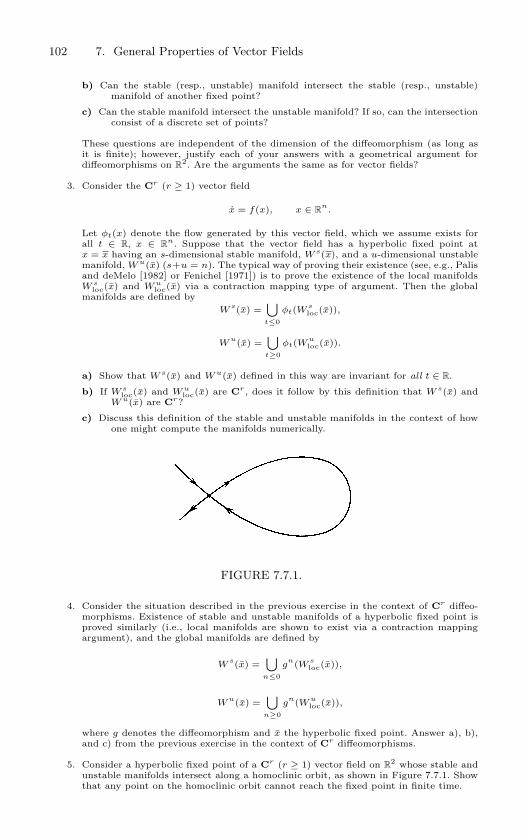
102 7. General Properties of Vector Fields
b) Can the stable (resp., unstable) manifold intersect the stable (resp., unstable)manifold of another fixed point?
c) Can the stable manifold intersect the unstable manifold? If so, can the intersectionconsist of a discrete set of points?
These questions are independent of the dimension of the diffeomorphism (as long asit is finite); however, justify each of your answers with a geometrical argument fordiffeomorphisms on R
2. Are the arguments the same as for vector fields?
3. Consider the Cr (r ≥ 1) vector field
x = f(x), x ∈ Rn
.
Let φt(x) denote the flow generated by this vector field, which we assume exists forall t ∈ R, x ∈ R
n. Suppose that the vector field has a hyperbolic fixed point atx = x having an s-dimensional stable manifold, W s(x), and a u-dimensional unstablemanifold, W u(x) (s+u = n). The typical way of proving their existence (see, e.g., Palisand deMelo [1982] or Fenichel [1971]) is to prove the existence of the local manifoldsW s
loc(x) and W uloc(x) via a contraction mapping type of argument. Then the global
manifolds are defined byW
s(x) =⋃t≤0
φt(Wsloc(x)),
Wu(x) =
⋃t≥0
φt(Wuloc(x)).
a) Show that W s(x) and W u(x) defined in this way are invariant for all t ∈ R.
b) If W sloc(x) and W u
loc(x) are Cr, does it follow by this definition that W s(x) andW u(x) are Cr?
c) Discuss this definition of the stable and unstable manifolds in the context of howone might compute the manifolds numerically.
FIGURE 7.7.1.
4. Consider the situation described in the previous exercise in the context of Cr diffeo-morphisms. Existence of stable and unstable manifolds of a hyperbolic fixed point isproved similarly (i.e., local manifolds are shown to exist via a contraction mappingargument), and the global manifolds are defined by
Ws(x) =
⋃n≤0
gn(W s
loc(x)),
Wu(x) =
⋃n≥0
gn(W u
loc(x)),
where g denotes the diffeomorphism and x the hyperbolic fixed point. Answer a), b),and c) from the previous exercise in the context of Cr diffeomorphisms.
5. Consider a hyperbolic fixed point of a Cr (r ≥ 1) vector field on R2 whose stable and
unstable manifolds intersect along a homoclinic orbit, as shown in Figure 7.7.1. Showthat any point on the homoclinic orbit cannot reach the fixed point in finite time.
7.7 Exercises 103
6. Consider a periodic orbit (of either a Cr (r ≥ 1) vector field or map) that is containedin a compact region of phase space. Can the period of the orbit be infinite?
7. Consider the Lorenz equations:
x = σ(y − x),y = ρx − y − xz,z = −βz + xy,
σ, β, ρ ≥ 0.
Describe the time evolution of volume elements under the flow generated by this vectorfield.
8. Does the divergence free property of a vector field imply that the vector field has afirst integral?
9. Consider the vector field:x = −x + sin t.
The solution through the point x0 at t0 is given by:
x(t; t0, x0) =12
(sin t − cos t) +(
x0 +12
cos t0 − 12
sin t0
)e
−(t−t0).
Construct a skew-product flow.
10. Consider the vector field:x = −x + t.
The solution through the point x0 at t0 is given by:
x(t; x0, t0) = t − 1 + (x0 − t0 + 1)e−(t−t0).
Construct a skew-product flow.
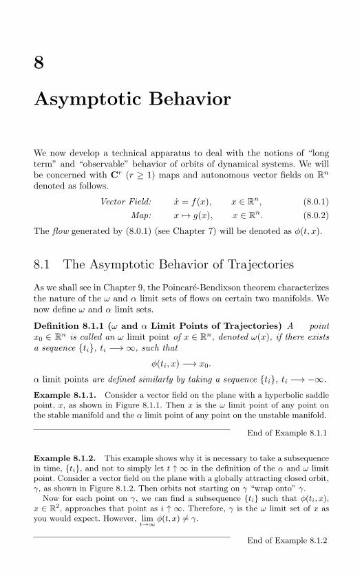
8
Asymptotic Behavior
We now develop a technical apparatus to deal with the notions of “longterm” and “observable” behavior of orbits of dynamical systems. We willbe concerned with Cr (r ≥ 1) maps and autonomous vector fields on R
n
denoted as follows.
Vector Field: x = f(x), x ∈ Rn, (8.0.1)
Map: x → g(x), x ∈ Rn. (8.0.2)
The flow generated by (8.0.1) (see Chapter 7) will be denoted as φ(t, x).
8.1 The Asymptotic Behavior of Trajectories
As we shall see in Chapter 9, the Poincare-Bendixson theorem characterizesthe nature of the ω and α limit sets of flows on certain two manifolds. Wenow define ω and α limit sets.
Definition 8.1.1 (ω and α Limit Points of Trajectories) A point
x0 ∈ Rn is called an ω limit point of x ∈ R
n, denoted ω(x), if there exists
a sequence ti, ti −→∞, such that
φ(ti, x) −→ x0.
α limit points are defined similarly by taking a sequence ti, ti −→ −∞.
Example 8.1.1. Consider a vector field on the plane with a hyperbolic saddle
point, x, as shown in Figure 8.1.1. Then x is the ω limit point of any point on
the stable manifold and the α limit point of any point on the unstable manifold.
End of Example 8.1.1
Example 8.1.2. This example shows why it is necessary to take a subsequence
in time, ti, and not to simply let t ↑ ∞ in the definition of the α and ω limit
point. Consider a vector field on the plane with a globally attracting closed orbit,
γ, as shown in Figure 8.1.2. Then orbits not starting on γ “wrap onto” γ.
Now for each point on γ, we can find a subsequence ti such that φ(ti, x),
x ∈ R2, approaches that point as i ↑ ∞. Therefore, γ is the ω limit set of x as
you would expect. However, limt→∞
φ(t, x) = γ.
End of Example 8.1.2
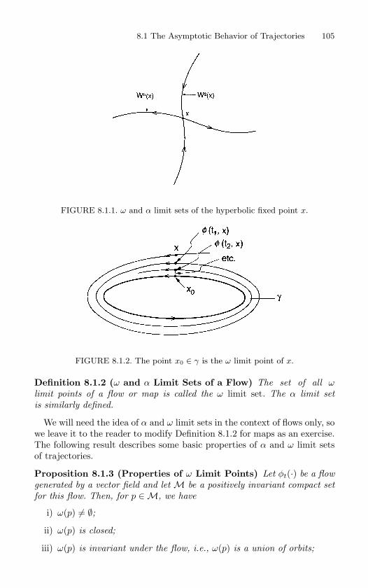
8.1 The Asymptotic Behavior of Trajectories 105
FIGURE 8.1.1. ω and α limit sets of the hyperbolic fixed point x.
FIGURE 8.1.2. The point x0 ∈ γ is the ω limit point of x.
Definition 8.1.2 (ω and α Limit Sets of a Flow) The set of all ωlimit points of a flow or map is called the ω limit set. The α limit set
is similarly defined.
We will need the idea of α and ω limit sets in the context of flows only, sowe leave it to the reader to modify Definition 8.1.2 for maps as an exercise.The following result describes some basic properties of α and ω limit setsof trajectories.
Proposition 8.1.3 (Properties of ω Limit Points) Let φt(·) be a flow
generated by a vector field and let M be a positively invariant compact set
for this flow. Then, for p ∈M, we have
i) ω(p) = ∅;
ii) ω(p) is closed;
iii) ω(p) is invariant under the flow, i.e., ω(p) is a union of orbits;
106 8. Asymptotic Behavior
iv) ω(p) is connected.
Proof: i) Choose a sequence ti, limi→∞
ti = ∞, and let pi = φti(p). Since
M is compact, pi has a convergent subsequence whose limit belongs toω(p). Thus, ω(p) = ∅.
ii) It suffices to show that the complement of ω(p) is open. Choose q ∈ω(p). Then there must exist some neighborhood of q, U(q), that is disjointfrom the set of points φt(p) | t ≥ T for some T > 0. Hence, q is containedin some open set that contains no points in ω(p). Since q is arbitrary, weare done.
iii) Let q ∈ ω(p) and q = φs(q). Choose a sequence ti −→ ∞ as i ↑ ∞with φti
(p) → q. Then φti+s(p) = φs
(φti
(p))
(cf. the notation for flowsfollowing Proposition 7.4.3) converges to q as i →∞. Hence, q ∈ ω(p), andtherefore ω(p) is invariant. However, there is a slight hole in this argumentthat needs to be filled; namely, it is not immediately obvious that φs(·)exists for all s.
We begin by arguing that φs(q) exists for s ∈ (−∞,∞) when q ∈ ω(p).It should be clear that this is true for s ∈ (0,∞) since M is a positivelyinvariant compact set (cf. Theorem 1.1.9). Therefore, it suffices to showthat this is true for s ∈ (−∞, 0].
Now q ∈ ω(p), so by definition we can find a sequence ti, ti −→ ∞ asi ↑ ∞, such that φti
(p) → q as i → ∞. Let us order the sequence so thatt1 < t2 < · · · < tn < · · · . Next consider φs
(φti(p)
). By Proposition 7.4.3
this is valid for s ∈ [−ti, 0]. Taking the limit as i →∞ and using continuityas well as the fact that φti → q as i → ∞, we see that φs(q) exists fors ∈ (−∞, 0].
iv) The proof is by contradiction. Suppose ω(p) is not connected. Thenwe can choose open sets V1, V2 such that ω(p) ⊂ V1 ∪ V2, ω(p) ∩ V1 = ∅,ω(p) ∩ V2 = ∅, and V1 ∩ V2 = ∅. The orbit of p accumulates on pointsin both V1 and V2; hence, for any given T > 0, there exists t > T suchthat φt(p) ∈ M− (V1 ∪ V2) = K. Therefore we can find a sequence tn,tn−→∞ as n ↑ ∞, with φtn
(p) ∈ K. Passing to a subsequence, if necessary(K is compact), we have φtn
(p) → q, q ∈ K. But this implies that q ∈V1 ∪ V2. However, our construction indicates that q is also in ω(p). This isa contradiction.
One can prove a similar result for α limit sets provided the hypothesesof the proposition are satisfied for the time reversed flow.
For maps, the notion of a nonwandering point has been more fashionable;however, we will explore the relationship between these two concepts in theexercises.
Definition 8.1.4 (Nonwandering Points) A point x0 is called nonwan-dering if the following holds.
8.2 Attracting Sets, Attractors, and Basins of Attraction 107
Flows: For any neighborhood U of x0 and T > 0, there exists some |t| > Tsuch that
φ(t, U) ∩ U = ∅.
Maps: For any neighborhood U of x0, there exists some n = 0 such that
gn(U) ∩ U = ∅.
Note that if the map is noninvertible, then we must take n > 0.
Fixed points and periodic orbits are nonwandering.
Definition 8.1.5 (Nonwandering Set) The set of all nonwandering
points of a map or flow is called the nonwandering set of that particular
map or flow.
8.2 Attracting Sets, Attractors, and Basins ofAttraction
Definitions 8.1.2 and 8.1.4 do not address the question of stability of thoseasymptotic motions. For this we want to develop the idea of an attractor.
Definition 8.2.1 (Attracting Set) A closed invariant set A ⊂ Rn is
called an attracting set if there is some neighborhood U of A such that:
flows: ∀t ≥ 0, φ(t, U) ⊂ U and⋂
t>0 φ(t, U) = A.
maps: ∀n ≥ 0, gn(U) ⊂ U and⋂
n>0 gn(U) = A.
Definition 8.2.2 (Trapping Region) The open set U in Definition
8.2.1 is often referred to as a trapping region.
A similar definition can be given for maps. By now the necessary modi-fications should be obvious, and we leave the details as an exercise for thereader.
It should be evident to the reader that finding a Liapunov function isequivalent to finding a trapping region (cf. Chapter 2). Also, let us mentiona technical point; by Theorem 7.1.1 it follows that all solutions starting ina trapping region exist for all positive times. This is useful in noncompactphase spaces such as R
2 for proving existence on semi-infinite time intervals.In the continuous time case, one “tests” whether or not a region is a
candidate to be a trapping region by evaluating the vector field on theboundary of the region in question. If, on the boundary of the region, thevector field is pointing toward the interior of the region, or is tangent tothe boundary, then the region in question is a trapping region. However,
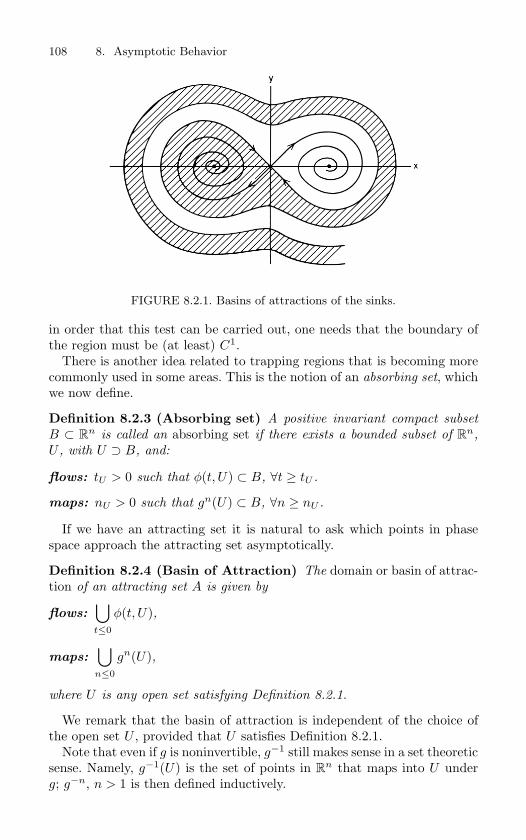
108 8. Asymptotic Behavior
FIGURE 8.2.1. Basins of attractions of the sinks.
in order that this test can be carried out, one needs that the boundary ofthe region must be (at least) C1.
There is another idea related to trapping regions that is becoming morecommonly used in some areas. This is the notion of an absorbing set, whichwe now define.
Definition 8.2.3 (Absorbing set) A positive invariant compact subset
B ⊂ Rn is called an absorbing set if there exists a bounded subset of R
n,
U , with U ⊃ B, and:
flows: tU > 0 such that φ(t, U) ⊂ B, ∀t ≥ tU .
maps: nU > 0 such that gn(U) ⊂ B, ∀n ≥ nU .
If we have an attracting set it is natural to ask which points in phasespace approach the attracting set asymptotically.
Definition 8.2.4 (Basin of Attraction) The domain or basin of attrac-tion of an attracting set A is given by
flows:⋃t≤0
φ(t, U),
maps:⋃n≤0
gn(U),
where U is any open set satisfying Definition 8.2.1.
We remark that the basin of attraction is independent of the choice ofthe open set U , provided that U satisfies Definition 8.2.1.
Note that even if g is noninvertible, g−1 still makes sense in a set theoreticsense. Namely, g−1(U) is the set of points in R
n that maps into U underg; g−n, n > 1 is then defined inductively.
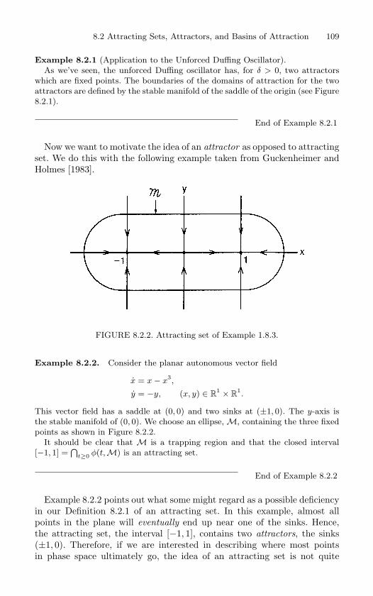
8.2 Attracting Sets, Attractors, and Basins of Attraction 109
Example 8.2.1 (Application to the Unforced Duffing Oscillator).
As we’ve seen, the unforced Duffing oscillator has, for δ > 0, two attractors
which are fixed points. The boundaries of the domains of attraction for the two
attractors are defined by the stable manifold of the saddle of the origin (see Figure
8.2.1).
End of Example 8.2.1
Now we want to motivate the idea of an attractor as opposed to attractingset. We do this with the following example taken from Guckenheimer andHolmes [1983].
FIGURE 8.2.2. Attracting set of Example 1.8.3.
Example 8.2.2. Consider the planar autonomous vector field
x = x − x3,
y = −y, (x, y) ∈ R1 × R
1.
This vector field has a saddle at (0, 0) and two sinks at (±1, 0). The y-axis is
the stable manifold of (0, 0). We choose an ellipse, M, containing the three fixed
points as shown in Figure 8.2.2.
It should be clear that M is a trapping region and that the closed interval
[−1, 1] =⋂
t≥0 φ(t, M) is an attracting set.
End of Example 8.2.2
Example 8.2.2 points out what some might regard as a possible deficiencyin our Definition 8.2.1 of an attracting set. In this example, almost allpoints in the plane will eventually end up near one of the sinks. Hence,the attracting set, the interval [−1, 1], contains two attractors, the sinks(±1, 0). Therefore, if we are interested in describing where most pointsin phase space ultimately go, the idea of an attracting set is not quite
110 8. Asymptotic Behavior
precise enough. Somehow we want to incorporate into the definition of anattracting set the notion that it is not a collection of distinct attractors,but rather that all points in the attracting set eventually come arbitrarilyclose to every other point in the attracting set under the evolution of theflow or map. We now want to make this mathematically precise.
Definition 8.2.5 (Topological Transitivity) A closed invariant set Ais said to be topologically transitive if, for any two open sets U , V ⊂ A
flows: ∃ t ∈ R φ(t, U) ∩ V = ∅,
maps: ∃ n ∈ Z gn(U) ∩ V = ∅.
Definition 8.2.6 (Attractor) An attractor is a topologically transitive
attracting set.
We remark that the study of attractors and their basin boundaries in dy-namical systems is rapidly evolving and, consequently, the theory is incom-plete. For more information see Conley [1978], Guckenheimer and Holmes[1983], Milnor [1985], and Ruelle [1981].
8.3 The LaSalle Invariance Principle
Here we describe an application of the invariance of ω limit sets of a trajec-tory that is very useful for stability issues. It is referred to as the LaSalle
invariance principle (LaSalle [1968]).We first develop the set-up. Let
x = f(x), x ∈ Rn,
denote a Cr, r ≥ 1 vector field. Let M ⊂ Rn be a positively invariant
compact set under the flow, φt(·), generated by this vector field, which isthe closure of some open set (so that it has nonempty interior) and whoseboundary is (at least) C1. Therefore M is a trapping region. Let V (x) bea Liapunov function on M. By this we mean that V ≤ 0 on M. Notethat we are using the term Liapunov function differently than was usedin Chapter 2. There Liapunov function was a local notion defined in theneighborhood of an equilibrium point. Now we will consider a more globalnotion. Consider the following two sets.
E ≡
x ∈M| V (x) = 0
,
M ≡
The union of all trajectories that start inEand remain in E for all t > 0.
M is the “positively invariant part” of E. Now we can state the LaSalleinvariance principle.
8.4 Attraction in Nonautonomous Systems 111
Theorem 8.3.1 (LaSalle, 1968) For all x ∈M, φt(x) → M as t →∞.
Proof: First we argue that V = χ = constant on ω(x) (see also Theorem15.0.3). This can be seen as follows. Suppose x ∈ ω(x) and let χ = V (x),then χ is the greatest lower bound of the set V (φt(x)) | t ≥ 0. This followsfrom the fact that V (x) decreases along trajectories (hence V (φti
(x)) ≥V (φt(x)) ≥ V (φti+1(x)) for ti ≤ t ≤ ti+1) and by the continuity of V (x).From Proposition 8.1.3 the omega limit set of a trajectory is invariant,hence φt(x) is also an omega limit point of φt(x). Then, since χ is thegreatest lower bound of the set V (φt(x)) | t ≥ 0, V (φt(x)) = χ.
From this it follows that V = 0 on ω(x). Then, by the definition of E,ω(x) ⊂ E. Since ω(x) is invariant (Proposition 8.1.3), it follows by thedefinition of M that ω(x) ⊂ M . Therefore, φt(x) → M as t →∞.
This result is particularly useful when one has information about M . Forexample, consider the Duffing equation
x = y,
y = x− x3 − δy, (x, y) ∈ R2, δ > 0.
Now consider the function
V (x, y) =y2
2− x2
2+
x4
4.
It is easy to verify thatV = −δy2.
Now consider the level set V = c for c very large, but finite. This curvedefines the boundary of a positively invariant compact set. E is given by theintersection of the x axis with this set and M is the three equilbrium pointson the x axis. The LaSalle invariance principle states that all trajectoriesconverge to one of the equilibrium points.
This example shows the relation between the Liapunov function V andthe trapping region M that often arises in specific applications. One firstconstructs a candidate for a Liapunov function. Then certain level sets ofthis function may be used to define M.
We remark that the LaSalle invariance principle can be generalized con-siderably. In particular, versions exist for situations where we have non-uniqueness of trajectories, finite time blow up of trajectories, and for dis-crete time dynamical systems, see LaSalle [1968] for details and references.
8.4 Attraction in Nonautonomous Systems
The notions of attracting set, basin of attraction, and attractor developedin this chapter may not be adequate to describe the same phenomena in
112 8. Asymptotic Behavior
nonautonomous systems. 1 In the nonautonomous setting attracting setsand basins of attraction may vary in time and the attraction rates mybe nonuniform. The paper of Kloeden and Schmalfuss [1997] is tutorial innature and provides an excellent introduction to the main issues. See alsoKloeden and Stonier [1998], Knyazhishche and Shavel [1995], Liu [1993],and Yoshizawa [1985].
We discuss some aspects of attraction in nonautonomous systems follow-ing Kloeden and Schmalfuss [1997] and Grune and Kloeden [2001].
First, for nonautonomous systems a different notion of convergence ofsolutions to a specific solution arises. We begin with some motivation forthis. Consider the following one-dimensional, linear nonautonomous vectorfield:
x = −x + g(t), x ∈ R. (8.4.1)
Using the variation of constants formula, it is easily computed that thetrajectory through the point x0 at t = t0 is given by:
x(t, t0, x0) = x0e−(t−t0) + e−t
∫ t
t0
esg(s)ds, (8.4.2)
where the function g(s) needs to be defined in such a way that the integralmakes sense, say continuous with no more than polynomial growth in s ass → ±∞.
It is a simple matter to conclude by examining (8.4.2) that all trajectoriesof (8.4.1) converge to the trajectory
φ(t) = e−t
∫ t
−∞esg(s)ds, (8.4.3)
as t → ∞ (the reader should verify that (8.4.3) is indeed a trajectory of(8.4.1)). This is called forward convergence and is mathematically expressedas:
limt→∞
|x(t, t0, x0)− φ(t)| = 0, t0, x0 fixed. (8.4.4)
Hence, forward convergence is a property that is verified in the limit ast → ∞. However, suppose we were interested in a different, but relatedquestion. Namely, for the trajectory φ(t), and a fixed, finite time t, char-acterize convergence of trajectories to φ(t) at the time t. This is a morepractical question from the point of view of applications, as well as numer-ical analysis, and give rise to the notion of pullback convergence, which ismathematically expressed as follows:
limt0→−∞
|x(t, t0, x0)− φ(t)| = 0, t, x0 fixed. (8.4.5)
1Of course, if the vector field is time periodic then one can reduce the problemto the study of a Poincare map (see Chapter 10) and then the results for mapsapply immediately.
8.4 Attraction in Nonautonomous Systems 113
Notice that (8.4.3) is the only trajectory which all trajectories of (8.4.1)converge to as t0 →∞ (with t fixed). However, there are many trajectoriesto which all trajectories of (8.4.1) converge to as t → ∞ (with t0 fixed).For example, all trajectories of (8.4.1) converge to
φ(t) = e−t
∫ t
t0
esg(s)ds,
for any fixed t0.For nonautonomous systems pullback convergence and forward conver-
gence are independent notions (see Exercises 16 and 17). However, they areequivalent for autonomous systems. Essentially this follows from Proposi-tion 7.4.1 which states that solutions of autonomous systems depend onlyon the “elapsed time”, t− t0. Hence, letting t →∞, with t0 fixed, is equiv-alent to letting t0 → −∞, with t fixed.
The history of pullback convergence is discussed briefly in Grune andKloeden [2001] who give much credit to the development of the idea toKrasnosel’skii [2001].
The notion of pullback convergence seems natural for defining attractorsin nonautonomous systems, as we now describe. First, we establish somegeneral notation. We begin by defining two notions of the distance betweencompact subsets of R
n.
Definition 8.4.1 (Hausdorff Separation) Let A and B be two non-
empty, compact subsets of Rn. The Hausdorff separation of A and B, de-
noted H∗(A, B), is defined as:
H∗(A, B) ≡ maxa∈A
dist (a,B) = maxa∈A
minb∈B
|a− b|. (8.4.6)
Now we can define the Hausdorff metric.
Definition 8.4.2 (Hausdorff Metric)
H(A, B) ≡ max (H∗(A, B), H∗(B, A)) . (8.4.7)
Now we can address the issue of attraction in the pullback sense usingthe language of cocycles developed in Chapter 7. Let φt,p, t ∈ R, p ∈ Pdenote a cocycle on R
n with respect to the group Θ of mappings on P (seeDefinition 7.5.1).
Definition 8.4.3 (Pullback Attracting Set) A family A = Ap, p ∈ Pof compact subsets of R
n is called a pullback attracting set of a cocycleφt,p, t ∈ R, p ∈ P on R
n if it is invariant in the sense that:
φt,p (Ap) = Aθtp, t ∈ R, p ∈ P,
114 8. Asymptotic Behavior
and pullback attracting in the sense that for every Ap there exists a bounded
subset of Rn, Dp ⊃ Ap, such that
limt→∞
H∗ (φt,θ−tp(Dθ−tp), Ap
)= 0.
The existence of a pullback attracting set is established through thenotion of a pullback absorbing family, which we now define (compare withthe definition of absorbing set given in Definition 8.2.3).
Definition 8.4.4 (Pullback Absorbing Family) A family
B = Bp, p ∈ P ,
of compact subsets of Rn is called a pullback absorbing family for a cocycle
φt,p, t ∈ R, p ∈ P on Rn if for each p ∈ P there is a bounded subset of
Rn, Up, satisfying Up ⊃ Bp, and a time tUp > 0 such that:
φt,θ−tp(Uθ−tp) ⊂ Bp, for all t ≥ tUp.
Now we can state the main theorem on the existence of pullback attract-ing sets.
Theorem 8.4.5 Let φt,p, t ∈ R, p ∈ P be a cocycle of continuous map-
pings on Rn with a pullback absorbing family B = Bp, p ∈ P. Then there
exists a pullback attracting set A = Ap, p ∈ P with components uniquely
determined by:
Ap =⋂τ≥0
⋃t≥τ
φt,θ−tp
(Bθ−tp
).
Various versions of this theorem are discussed in Grune and Kloeden[2001], where the notion of Lyapunov functions for pullback attracting setsis also discussed.
8.5 Exercises1. Let φt(x) denote a flow generated by a Cr (r ≥ 1) vector field on R
n that exists forall x ∈ R
n, t ∈ R.
1) Show that the α and ω limit sets of the flow are contained in the nonwanderingset of the flow.
2) Is the nonwandering set contained in the union of the α and ω limit set?
2. Prove that the basin of attraction is independent of the choice of the open set U ,provided that U satisfies Definition 8.2.1.
3. Suppose A is an attracting set (of either a vector field or map), and suppose that x ∈ Ais a hyperbolic fixed point of saddle-type. Must the following be true
8.5 Exercises 115
1) W s(x) ⊂ A,
2) W u(x) ⊂ A?
4. Consider the union of the homoclinic orbit and the hyperbolic fixed point that itconnects (shown in Figure 7.7.1). Can this set be an attracting set?
5. Consider the Cr (r ≥ 1) diffeomorphism
x → g(x), x ∈ Rn
.
Suppose that det Dg(x) = 1 ∀ x ∈ Rn. Prove that the diffeomorphism preserves volume.
6. Consider the following vector field on R2.
(x1x2
)=(
−λ 00 λ
)(x1x2
), λ > 0.
The stable manifold of the origin is given by
Ws(0, 0) =
(x1, x2) ∈ R
2 | x2 = 0
.
Consider a line segment contained in W s(0, 0). Under the evolution of the flow gener-ated by the vector field the length of the line segment shrinks to zero as t → ∞. Doesthis violate the result of Exercise 5? Why or why not?
7. Consider the Cr (r ≥ 1) diffeomorphism
x → g(x), x ∈ Rn
.
Suppose x = x is a nonwandering point, i.e., for any neighborhood U of x, there existsan n = 0 such that gn(U) ∩ U = ∅ (cf. Definition 8.1.4). Is it possible that there mayexist only one such n, or, if there exists one n, must there be a countable (infinity?)of such n? Does the same result hold for flows?
8. Let B be an absorbing set. Show that:
⋂t≥0
φ(t, B),
is an attracting set.
9. Describe the relation between trapping regions and absorbing sets.
10. Apply the LaSalle Invariance principle to the vector field
x = x − x3,
y = −y, (x, y) ∈ R2,
and conclude that all trajectories converge to one of the equilibrium points.
11. Consider the simple harmonic oscillator
x = y,
y = −x, (x, y) ∈ R2.
Using
V (x, y) =12
(x2 + y
2)
,
as a Liapunov function, what does the LaSalle invariance principle say about thissystem?
116 8. Asymptotic Behavior
12. Suppose that M is a positively invariant compact set for a flow φt(·), which is theclosure of some open set and has a C1 boundary, and that V is a strict Liapunovfunction on M − equilibrium points. Then show that all trajectories converge to anequilibrium point.
13. With M and M defined as in the discussion of the LaSalle invariance principle, if Vis a Liapunov function on M show that M is an attracting set and the interior of Mis in the basin of attraction.
14. Suppose x(t, t0, x0) is a trajectory of an autonomous vector field in Rn that exists for
all time. Consider the set
T =
x ∈ Rn | x = x(t, t0, x0), t ∈ R
.
Prove that T is an invariant set.
15. Suppose x(t, t0, x0) is a trajectory of an nonautonomous vector field in Rn that exists
for all time. Consider the set
T =
x ∈ Rn | x = x(t, t0, x0), t ∈ R
.
Argue that T is not generally an invariant set.
16. Consider the vector field:x = −2tx, x ∈ R.
Show that all trajectories are forward, but not pullback, convergent to x = 0.
17. Consider the vector field:x = 2tx, x ∈ R.
Show that all trajectories are pullback, but not forward, convergent to x = 0.
18. Reformulate Definition 8.4.3 in terms of the trajectories of nonautonomous vectorfields.
19. Reformulate Definition 8.4.4 in terms of the trajectories of nonautonomous vectorfields.
20. Reformulate Theorem 8.4.5 in terms of the trajectories of nonautonomous vector fields.
21. Consider the vector field:x = −x + sin t.
The solution through the point x0 at t0 is given by:
x(t; t0, x0) =12
(sin t − cos t) +(
x0 +12
cos t0 − 12
sin t0
)e
−(t−t0).
Construct the pullback attracting set.
22. Consider the vector field:x = −x + t.
The solution through the point x0 at t0 is given by:
x(t; x0, t0) = t − 1 + (x0 − t0 + 1)e−(t−t0).
Construct the pullback attracting set.
23. Prove Theorem 8.4.5.
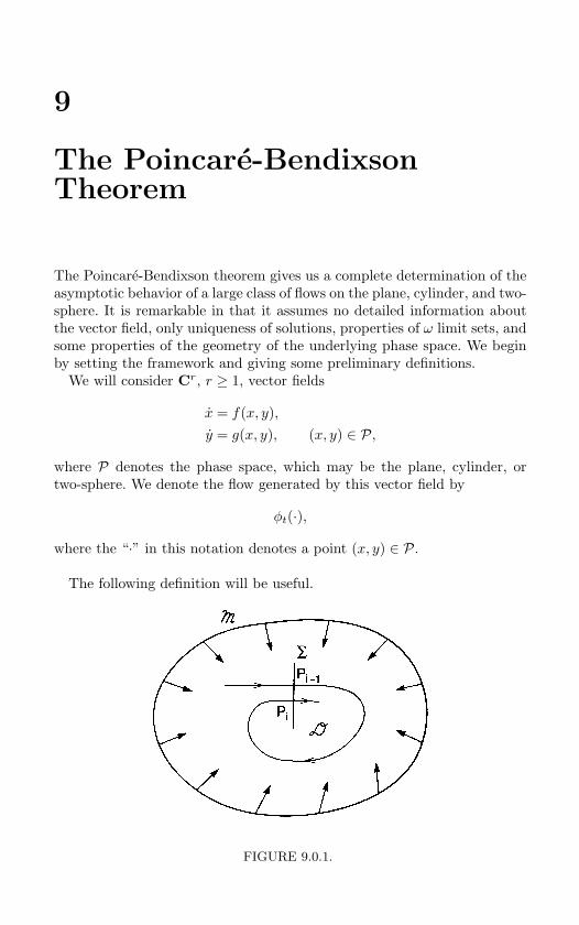
9
The Poincare-BendixsonTheorem
The Poincare-Bendixson theorem gives us a complete determination of theasymptotic behavior of a large class of flows on the plane, cylinder, and two-sphere. It is remarkable in that it assumes no detailed information aboutthe vector field, only uniqueness of solutions, properties of ω limit sets, andsome properties of the geometry of the underlying phase space. We beginby setting the framework and giving some preliminary definitions.
We will consider Cr, r ≥ 1, vector fields
x = f(x, y),y = g(x, y), (x, y) ∈ P,
where P denotes the phase space, which may be the plane, cylinder, ortwo-sphere. We denote the flow generated by this vector field by
φt(·),
where the “·” in this notation denotes a point (x, y) ∈ P.
The following definition will be useful.
FIGURE 9.0.1.
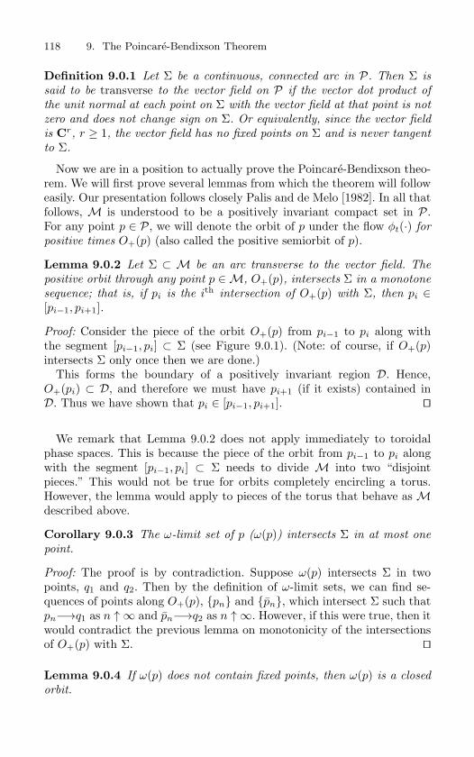
118 9. The Poincare-Bendixson Theorem
Definition 9.0.1 Let Σ be a continuous, connected arc in P. Then Σ is
said to be transverse to the vector field on P if the vector dot product of
the unit normal at each point on Σ with the vector field at that point is not
zero and does not change sign on Σ. Or equivalently, since the vector field
is Cr, r ≥ 1, the vector field has no fixed points on Σ and is never tangent
to Σ.
Now we are in a position to actually prove the Poincare-Bendixson theo-rem. We will first prove several lemmas from which the theorem will followeasily. Our presentation follows closely Palis and de Melo [1982]. In all thatfollows, M is understood to be a positively invariant compact set in P.For any point p ∈ P, we will denote the orbit of p under the flow φt(·) for
positive times O+(p) (also called the positive semiorbit of p).
Lemma 9.0.2 Let Σ ⊂ M be an arc transverse to the vector field. The
positive orbit through any point p ∈M, O+(p), intersects Σ in a monotone
sequence; that is, if pi is the ith intersection of O+(p) with Σ, then pi ∈[pi−1, pi+1].
Proof: Consider the piece of the orbit O+(p) from pi−1 to pi along withthe segment [pi−1, pi] ⊂ Σ (see Figure 9.0.1). (Note: of course, if O+(p)intersects Σ only once then we are done.)
This forms the boundary of a positively invariant region D. Hence,O+(pi) ⊂ D, and therefore we must have pi+1 (if it exists) contained inD. Thus we have shown that pi ∈ [pi−1, pi+1].
We remark that Lemma 9.0.2 does not apply immediately to toroidalphase spaces. This is because the piece of the orbit from pi−1 to pi alongwith the segment [pi−1, pi] ⊂ Σ needs to divide M into two “disjointpieces.” This would not be true for orbits completely encircling a torus.However, the lemma would apply to pieces of the torus that behave as Mdescribed above.
Corollary 9.0.3 The ω-limit set of p (ω(p)) intersects Σ in at most one
point.
Proof: The proof is by contradiction. Suppose ω(p) intersects Σ in twopoints, q1 and q2. Then by the definition of ω-limit sets, we can find se-quences of points along O+(p), pn and pn, which intersect Σ such thatpn−→q1 as n ↑ ∞ and pn−→q2 as n ↑ ∞. However, if this were true, then itwould contradict the previous lemma on monotonicity of the intersectionsof O+(p) with Σ.
Lemma 9.0.4 If ω(p) does not contain fixed points, then ω(p) is a closed
orbit.
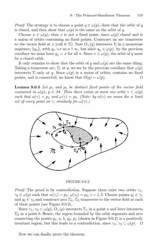
9. The Poincare-Bendixson Theorem 119
Proof: The strategy is to choose a point q ∈ ω(p), show that the orbit of qis closed, and then show that ω(p) is the same as the orbit of q.
Choose x ∈ ω(q); then x is not a fixed point, since ω(p) closed and isa union of orbits containing no fixed points. Construct an arc transverseto the vector field at x (call it Σ). Now O+(q) intersects Σ in a monotonesequence, qn, with qn→x as n ↑ ∞, but since qn ∈ ω(p), by the previouscorollary we must have qn = x for all n. Since x ∈ ω(q), the orbit of q mustbe a closed orbit.
It only remains to show that the orbit of q and ω(p) are the same thing.Taking a transverse arc, Σ, at q, we see by the previous corollary that ω(p)intersects Σ only at q. Since ω(p) is a union of orbits, contains no fixedpoints, and is connected, we know that O(q) = ω(p).
Lemma 9.0.5 Let p1 and p2 be distinct fixed points of the vector field
contained in ω(p), p ∈ M. Then there exists at most one orbit γ ⊂ ω(p)such that α(γ) = p1 and ω(γ) = p2. (Note: by α(γ) we mean the α limit
set of every point on γ; similarly for ω(γ).)
FIGURE 9.0.2.
Proof: The proof is by contradiction. Suppose there exist two orbits γ1,γ2 ∈ ω(p) such that α(γi) = p1, ω(γi) = p2, i = 1, 2. Choose points q1 ∈ γ1and q2 ∈ γ2 and construct arcs Σ1, Σ2 transverse to the vector field at eachof these points (see Figure 9.0.2).
Since γ1, γ2 ⊂ ω(p), O+(p) intersects Σ1 in a point a and later intersectsΣ2 in a point b. Hence, the region bounded by the orbit segments and arcsconnecting the points q1, a, b, q2, p2 (shown in Figure 9.0.2) is a positivelyinvariant region, but this leads to a contradiction, since γ1, γ2 ⊂ ω(p).
Now we can finally prove the theorem.
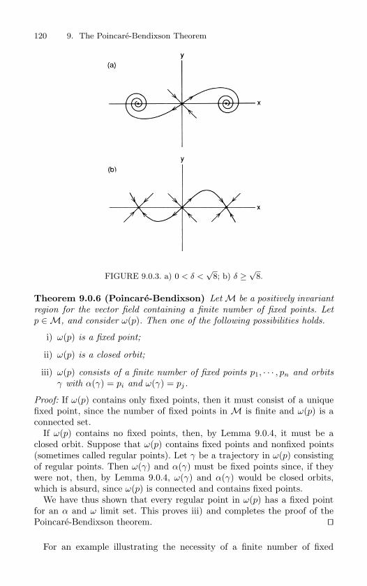
120 9. The Poincare-Bendixson Theorem
FIGURE 9.0.3. a) 0 < δ <√
8; b) δ ≥ √8.
Theorem 9.0.6 (Poincare-Bendixson) Let M be a positively invariant
region for the vector field containing a finite number of fixed points. Let
p ∈M, and consider ω(p). Then one of the following possibilities holds.
i) ω(p) is a fixed point;
ii) ω(p) is a closed orbit;
iii) ω(p) consists of a finite number of fixed points p1, · · · , pn and orbits
γ with α(γ) = pi and ω(γ) = pj.
Proof: If ω(p) contains only fixed points, then it must consist of a uniquefixed point, since the number of fixed points in M is finite and ω(p) is aconnected set.
If ω(p) contains no fixed points, then, by Lemma 9.0.4, it must be aclosed orbit. Suppose that ω(p) contains fixed points and nonfixed points(sometimes called regular points). Let γ be a trajectory in ω(p) consistingof regular points. Then ω(γ) and α(γ) must be fixed points since, if theywere not, then, by Lemma 9.0.4, ω(γ) and α(γ) would be closed orbits,which is absurd, since ω(p) is connected and contains fixed points.
We have thus shown that every regular point in ω(p) has a fixed pointfor an α and ω limit set. This proves iii) and completes the proof of thePoincare-Bendixson theorem.
For an example illustrating the necessity of a finite number of fixed
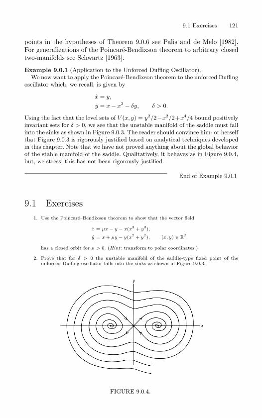
9.1 Exercises 121
points in the hypotheses of Theorem 9.0.6 see Palis and de Melo [1982].For generalizations of the Poincare-Bendixson theorem to arbitrary closedtwo-manifolds see Schwartz [1963].
Example 9.0.1 (Application to the Unforced Duffing Oscillator).
We now want to apply the Poincare-Bendixson theorem to the unforced Duffing
oscillator which, we recall, is given by
x = y,
y = x − x3 − δy, δ > 0.
Using the fact that the level sets of V (x, y) = y2/2−x2/2+x4/4 bound positively
invariant sets for δ > 0, we see that the unstable manifold of the saddle must fall
into the sinks as shown in Figure 9.0.3. The reader should convince him- or herself
that Figure 9.0.3 is rigorously justified based on analytical techniques developed
in this chapter. Note that we have not proved anything about the global behavior
of the stable manifold of the saddle. Qualitatively, it behaves as in Figure 9.0.4,
but, we stress, this has not been rigorously justified.
End of Example 9.0.1
9.1 Exercises1. Use the Poincare–Bendixson theorem to show that the vector field
x = µx − y − x(x2 + y2),
y = x + µy − y(x2 + y2), (x, y) ∈ R
2,
has a closed orbit for µ > 0. (Hint: transform to polar coordinates.)
2. Prove that for δ > 0 the unstable manifold of the saddle-type fixed point of theunforced Duffing oscillator falls into the sinks as shown in Figure 9.0.3.
FIGURE 9.0.4.
10
Poincare Maps
The idea of reducing the study of continuous time systems (flows) to thestudy of an associated discrete time system (map) is due to Poincare [1899],who first utilized it in his studies of the three body problem in celestialmechanics. Nowadays virtually any discrete time system that is associatedwith an ordinary differential equation is referred to as a Poincare map.This technique offers several advantages in the study of ordinary differentialequations, including the following:
1. Dimensional Reduction. Construction of the Poincare map involvesthe elimination of at least one of the variables of the problem resultingin the study of a lower dimensional problem.
2. Global Dynamics. In lower dimensional problems (say, dimension ≤ 4)numerically computed Poincare maps provide an insightful and strik-ing display of the global dynamics of a system; see Guckenheimer andHolmes [1983] and Lichtenberg and Lieberman [1982] for examples ofnumerically computed Poincare maps.
3. Conceptual Clarity . Many concepts that are somewhat cumbersometo state for ordinary differential equations may often be succinctlystated for the associated Poincare map. An example would be thenotion of orbital stability of a periodic orbit of an ordinary differentialequation (see Hale [1980]). In terms of the Poincare map, this problemwould reduce to the problem of the stability of a fixed point of themap, which is simply characterized in terms of the eigenvalues of themap linearized about the fixed point.
It would be useful to give methods for constructing the Poincare map as-sociated with an ordinary differential equation. Unfortunately, there existno general methods applicable to arbitrary ordinary differential equations,since construction of the Poincare map requires some knowledge of thegeometrical structure of the phase space of the ordinary differential equa-tion. Thus, construction of a Poincare map requires ingenuity specific tothe problem at hand; however, in four cases that come up frequently, theconstruction of a specific type of Poincare map can in some sense be saidto be canonical. The four cases are:
1. In the study of the orbit structure near a periodic orbit of an ordinarydifferential equation.
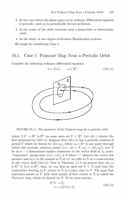
10.1 Poincare Map Near a Periodic Orbit 123
2. In the case where the phase space of an ordinary differential equationis periodic, such as in periodically forced oscillators.
3. In the study of the orbit structure near a homoclinic or heteroclinicorbit.
4. In the study of two degree-of-freedom Hamiltonian systems.
We begin by considering Case 1.
10.1 Case 1: Poincare Map Near a Periodic Orbit
Consider the following ordinary differential equation
x = f(x), x ∈ Rn, (10.1.1)
FIGURE 10.1.1. The geometry of the Poincare map for a periodic orbit.
where f :U → Rn is Cr on some open set U ⊂ R
n. Let φ(t, ·) denote theflow generated by (10.1.1). Suppose that (10.1.1) has a periodic solution ofperiod T which we denote by φ(t, x0), where x0 ∈ R
n is any point throughwhich this periodic solution passes (i.e., φ(t + T, x0) = φ(t, x0)). Let Σbe an n− 1 dimensional surface transverse to the vector field at x0 (note:“transverse” means that f(x) · n(x) = 0 where “·” denotes the vector dotproduct and n(x) is the normal to Σ at x); we refer to Σ as a cross-sectionto the vector field (10.1.1). Now in Theorem 7.1.1 we proved that φ(t, x)is Cr if f(x) is Cr; thus, we can find an open set V ⊂ Σ such that thetrajectories starting in V return to Σ in a time close to T . The map thatassociates points in V with their points of first return to Σ is called thePoincare map, which we denote by P . To be more precise,
P : V → Σ,x → φ
(τ(x), x
),
(10.1.2)
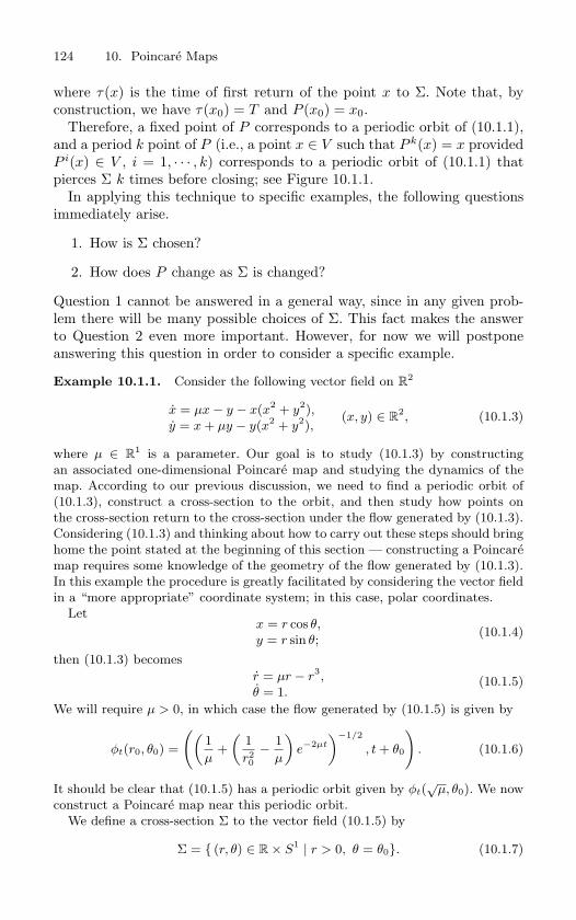
124 10. Poincare Maps
where τ(x) is the time of first return of the point x to Σ. Note that, byconstruction, we have τ(x0) = T and P (x0) = x0.
Therefore, a fixed point of P corresponds to a periodic orbit of (10.1.1),and a period k point of P (i.e., a point x ∈ V such that P k(x) = x providedP i(x) ∈ V , i = 1, · · · , k) corresponds to a periodic orbit of (10.1.1) thatpierces Σ k times before closing; see Figure 10.1.1.
In applying this technique to specific examples, the following questionsimmediately arise.
1. How is Σ chosen?
2. How does P change as Σ is changed?
Question 1 cannot be answered in a general way, since in any given prob-lem there will be many possible choices of Σ. This fact makes the answerto Question 2 even more important. However, for now we will postponeanswering this question in order to consider a specific example.
Example 10.1.1. Consider the following vector field on R2
x = µx − y − x(x2+ y2
),y = x + µy − y(x2
+ y2),
(x, y) ∈ R2, (10.1.3)
where µ ∈ R1 is a parameter. Our goal is to study (10.1.3) by constructing
an associated one-dimensional Poincare map and studying the dynamics of the
map. According to our previous discussion, we need to find a periodic orbit of
(10.1.3), construct a cross-section to the orbit, and then study how points on
the cross-section return to the cross-section under the flow generated by (10.1.3).
Considering (10.1.3) and thinking about how to carry out these steps should bring
home the point stated at the beginning of this section — constructing a Poincare
map requires some knowledge of the geometry of the flow generated by (10.1.3).
In this example the procedure is greatly facilitated by considering the vector field
in a “more appropriate” coordinate system; in this case, polar coordinates.
Letx = r cos θ,y = r sin θ;
(10.1.4)
then (10.1.3) becomes
r = µr − r3,θ = 1.
(10.1.5)
We will require µ > 0, in which case the flow generated by (10.1.5) is given by
φt(r0, θ0) =
((1
µ+
(1
r20
− 1
µ
)e−2µt
)−1/2
, t + θ0
). (10.1.6)
It should be clear that (10.1.5) has a periodic orbit given by φt(√
µ, θ0). We now
construct a Poincare map near this periodic orbit.
We define a cross-section Σ to the vector field (10.1.5) by
Σ = (r, θ) ∈ R × S1 | r > 0, θ = θ0. (10.1.7)
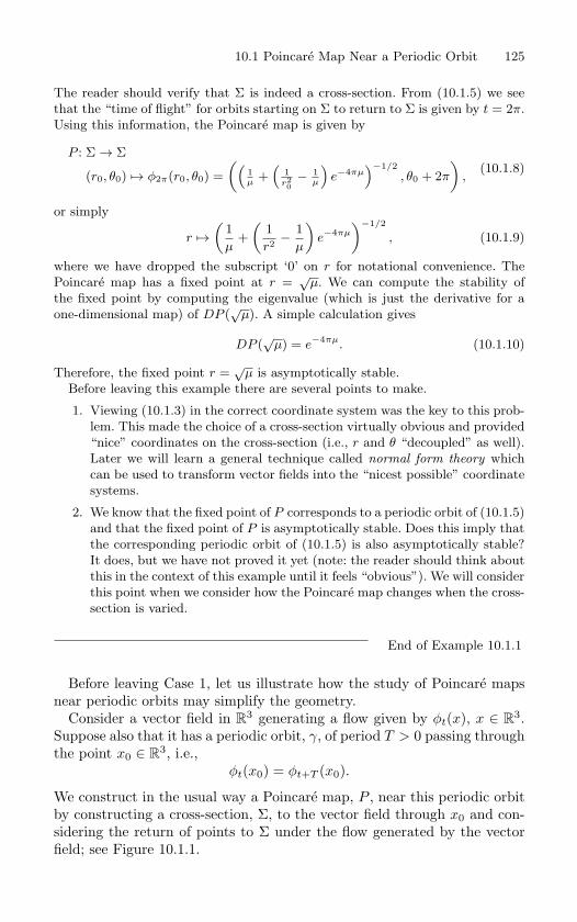
10.1 Poincare Map Near a Periodic Orbit 125
The reader should verify that Σ is indeed a cross-section. From (10.1.5) we see
that the “time of flight” for orbits starting on Σ to return to Σ is given by t = 2π.
Using this information, the Poincare map is given by
P : Σ → Σ
(r0, θ0) → φ2π(r0, θ0) =
((1µ
+(
1r20
− 1µ
)e−4πµ
)−1/2, θ0 + 2π
),
(10.1.8)
or simply
r →(
1
µ+
(1
r2 − 1
µ
)e−4πµ
)−1/2
, (10.1.9)
where we have dropped the subscript ‘0’ on r for notational convenience. The
Poincare map has a fixed point at r =√
µ. We can compute the stability of
the fixed point by computing the eigenvalue (which is just the derivative for a
one-dimensional map) of DP (√
µ). A simple calculation gives
DP (√
µ) = e−4πµ. (10.1.10)
Therefore, the fixed point r =√
µ is asymptotically stable.
Before leaving this example there are several points to make.
1. Viewing (10.1.3) in the correct coordinate system was the key to this prob-
lem. This made the choice of a cross-section virtually obvious and provided
“nice” coordinates on the cross-section (i.e., r and θ “decoupled” as well).
Later we will learn a general technique called normal form theory which
can be used to transform vector fields into the “nicest possible” coordinate
systems.
2. We know that the fixed point of P corresponds to a periodic orbit of (10.1.5)
and that the fixed point of P is asymptotically stable. Does this imply that
the corresponding periodic orbit of (10.1.5) is also asymptotically stable?
It does, but we have not proved it yet (note: the reader should think about
this in the context of this example until it feels “obvious”). We will consider
this point when we consider how the Poincare map changes when the cross-
section is varied.
End of Example 10.1.1
Before leaving Case 1, let us illustrate how the study of Poincare mapsnear periodic orbits may simplify the geometry.
Consider a vector field in R3 generating a flow given by φt(x), x ∈ R
3.Suppose also that it has a periodic orbit, γ, of period T > 0 passing throughthe point x0 ∈ R
3, i.e.,φt(x0) = φt+T (x0).
We construct in the usual way a Poincare map, P , near this periodic orbitby constructing a cross-section, Σ, to the vector field through x0 and con-sidering the return of points to Σ under the flow generated by the vectorfield; see Figure 10.1.1.
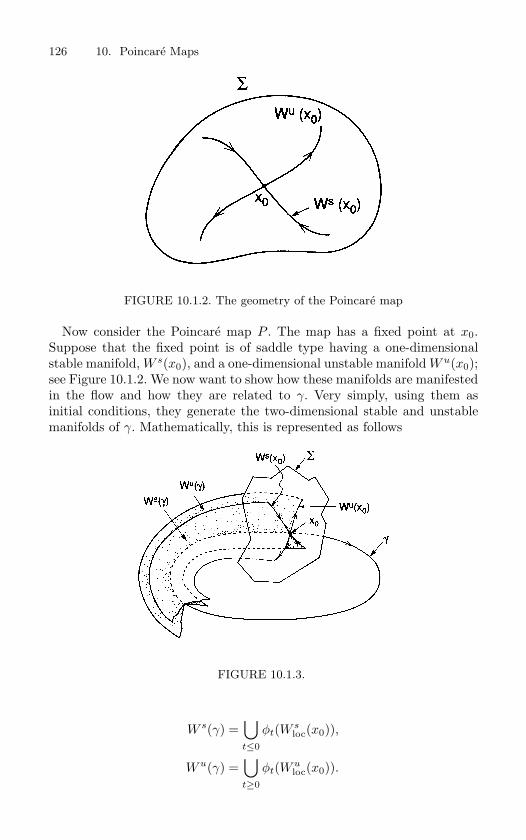
126 10. Poincare Maps
FIGURE 10.1.2. The geometry of the Poincare map
Now consider the Poincare map P . The map has a fixed point at x0.Suppose that the fixed point is of saddle type having a one-dimensionalstable manifold, W s(x0), and a one-dimensional unstable manifold Wu(x0);see Figure 10.1.2. We now want to show how these manifolds are manifestedin the flow and how they are related to γ. Very simply, using them asinitial conditions, they generate the two-dimensional stable and unstablemanifolds of γ. Mathematically, this is represented as follows
FIGURE 10.1.3.
W s(γ) =⋃t≤0
φt(W sloc(x0)),
Wu(γ) =⋃t≥0
φt(Wuloc(x0)).
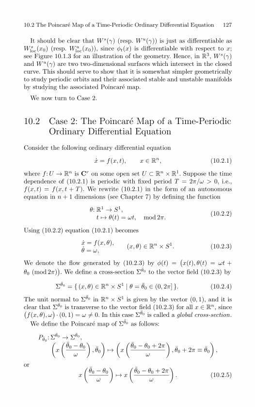
10.2 The Poincare Map of a Time-Periodic Ordinary Differential Equation 127
It should be clear that W s(γ) (resp. Wu(γ)) is just as differentiable asW s
loc(x0) (resp. Wuloc(x0)), since φt(x) is differentiable with respect to x;
see Figure 10.1.3 for an illustration of the geometry. Hence, in R3, W s(γ)
and Wu(γ) are two two-dimensional surfaces which intersect in the closedcurve. This should serve to show that it is somewhat simpler geometricallyto study periodic orbits and their associated stable and unstable manifoldsby studying the associated Poincare map.
We now turn to Case 2.
10.2 Case 2: The Poincare Map of a Time-PeriodicOrdinary Differential Equation
Consider the following ordinary differential equation
x = f(x, t), x ∈ Rn, (10.2.1)
where f :U → Rn is Cr on some open set U ⊂ R
n × R1. Suppose the time
dependence of (10.2.1) is periodic with fixed period T = 2π/ω > 0, i.e.,f(x, t) = f(x, t + T ). We rewrite (10.2.1) in the form of an autonomousequation in n + 1 dimensions (see Chapter 7) by defining the function
θ: R1 → S1,
t → θ(t) = ωt, mod 2π.(10.2.2)
Using (10.2.2) equation (10.2.1) becomes
x = f(x, θ),θ = ω,
(x, θ) ∈ Rn × S1. (10.2.3)
We denote the flow generated by (10.2.3) by φ(t) =(x(t), θ(t) = ωt +
θ0 (mod 2π)). We define a cross-section Σθ0 to the vector field (10.2.3) by
Σθ0 = (x, θ) ∈ Rn × S1 | θ = θ0 ∈ (0, 2π] . (10.2.4)
The unit normal to Σθ0 in Rn × S1 is given by the vector (0, 1), and it is
clear that Σθ0 is transverse to the vector field (10.2.3) for all x ∈ Rn, since(
f(x, θ), ω)· (0, 1) = ω = 0. In this case Σθ0 is called a global cross-section.
We define the Poincare map of Σθ0 as follows:
Pθ0: Σθ0 → Σθ0 ,(
x
(θ0 − θ0
ω
), θ0
)→
(x
(θ0 − θ0 + 2π
ω
), θ0 + 2π ≡ θ0
),
or
x
(θ0 − θ0
ω
)→ x
(θ0 − θ0 + 2π
ω
). (10.2.5)
128 10. Poincare Maps
Thus, the Poincare map merely tracks initial conditions in x at a fixedphase after successive periods of the vector field.
It should be clear that fixed points Pθ0correspond to 2π/ω-periodic
orbits of (10.2.1) and k-periodic points of Pθ0correspond to periodic orbits
of (10.2.1) that pierce Σθ0 k times before closing. We will worry about theeffect on the dynamics of the map caused by changing the cross-sectionlater. Now we consider an example.
10.2a Periodically Forced Linear OscillatorsConsider the following ordinary differential equation
x + δx + ω20x = γ cos ωt. (10.2.6)
This is an equation which most students learn to solve in elementary cal-culus courses. Our goal here is to study the nature of solutions of (1.2.17)from our more geometrical setting in the context of Poincare maps. Thiswill enable the reader to obtain a new point of view on something relativelyfamiliar and, we hope, to see the value of this new point of view.
We begin by first obtaining the solution of (10.2.6). Recall (see, e.g.,Arnold [1973] or Hirsch and Smale [1974]) that the general solution of(1.2.17) is the sum of the solution of the homogeneous equation (i.e., thesolution for γ = 0), sometimes called the free oscillation, and a particularsolution, sometimes called the forced oscillation. For δ > 0 there are severalpossibilities for the homogeneous solution, which we state below.
δ > 0: The Homogeneous Solution, xh(t)
There are three cases depending on the sign of the quantity δ2 − 4ω20 .
(a) δ2 − 4ω20 > 0 ⇒ xh(t) = C1e
r1t + C2er2t, (10.2.7)
wherer1,2 = −δ/2± (1/2)
√δ2 − 4ω2
0 ,
(b) δ2 − 4ω20 = 0 ⇒ xh(t) = (C1 + C2t)e−(δ/2)t,
(c) δ2 − 4ω20 < 0 ⇒ xh(t) = e−(δ/2)t(C1 cos ωt + C2 sin ωt),
and where ω = (1/2)√
4ω20 − δ2. In all three cases C1 and C2 are unknown
constants which are fixed when initial conditions are specified. Also, no-tice that in all three cases lim
t→∞xh(t) = 0. We now turn to the particular
solution.
10.2 The Poincare Map of a Time-Periodic Ordinary Differential Equation 129
The Particular Solution, xp(t)
The particular solution is given by
xp(t) = A cos ωt + B sin ωt, (10.2.8)
where
A ≡ (ω20 − ω2)γ
(ω20 − ω2)2 + (δω)2
, B ≡ δγω
(ω20 − ω2)2 + (δω)2
.
Next we turn to the construction of the Poincare map. For this we willconsider only the case δ2 − 4ω2
0 < 0. The other two cases are similar, andwe leave them as exercises for the reader.
The Poincare Map: δ2 − 4ω20 < 0
Rewriting (10.2.6) as a system, we obtain
x = y,y = −ω2
0x− δy + γ cos ωt.(10.2.9)
By rewriting (10.2.9) as an autonomous system, as was described at thebeginning of our discussion of Case 2, we obtain
x = y,y = −ω2
0x− δy + γ cos θ,θ = ω,
(x, y, θ) ∈ R1 × R
1 × S1. (10.2.10)
The flow generated by (10.2.10) is given by
φt(x0, y0, θ0) =(x(t), y(t), ωt + θ0
), (10.2.11)
where, using (10.2.7c) and (10.2.8), x(t) is given by
x(t) = e−(δ/2)t(C1 cos ωt + C2 sin ωt) + A cos ωt + B sinωt
withy(t) = x(t). (10.2.12)
The constants C1 and C2 are obtained by requiring
x(0) = x0,y(0) = y0,
which yieldC1 = x0 −A,
C2 =1ω
(δ
2x0 + y0 −
δ
2A− ωB
). (10.2.13)
Notice from (10.2.9) that we can set θ0 = 0 in (10.2.11) (cf. (10.2.5)).
130 10. Poincare Maps
We construct a cross-section at θ0 = 0 (note: this is why we specified theinitial conditions at t = 0) as follows
Σ0 ≡ Σ = (x, y, θ) ∈ R1 × R
1 × S1 | θ = 0 ∈ [0, 2π) , (10.2.14)
where we have dropped the subscript “0” on x, y, and θ for notationalconvenience. Using (10.2.12), the Poincare map is given by
P : Σ → Σ,(xy
)→ e−δπ/ω
( C + δ2ωS 1
ωS−ω2
0ω S C − δ
2ωS
)(xy
)
+
(e−δπ/ω
[−AC +
(− δ
2ω A− ωω B
)S]+ A
e−δπ/ω[−ωBC +
(ω2
0ω A + δω
2ω B)S]
+ ωB
),
(10.2.15)
where
C ≡ cos 2πω
ω,
S ≡ sin 2πω
ω.
Equation (10.2.15) is an example of an affine map, i.e., it is linear mapplus a translation.
The Poincare map has a single fixed point given by
(x, y) = (A, ωB) (10.2.16)
(note: this should not be surprising). The next question is whether or notthe fixed point is stable. A simple calculation shows that the eigenvaluesof DP (A, ωB) are given by
λ1,2 = e−δπ/ω±i2πω/ω. (10.2.17)
Thus the fixed point is asymptotically stable with nearby orbits appear-ing as in Figure 10.2.1. (Note: the “spiraling” of orbits near the fixed pointis due to the imaginary part of the eigenvalues.) Figure 10.2.1 is drawn forA > 0; see (10.2.8).
The Case of Resonance: ω = ω
We now consider the situation where the driving frequency is equal to thefrequency of the free oscillation. In this case the the Poincare map becomes
P : Σ → Σ,(xy
)→ e−δπ/ω
(1 00 1
)(xy
)+
(A(1− e−δπ/ω)
ωB(1− e−δπ/ω)
).
(10.2.18)
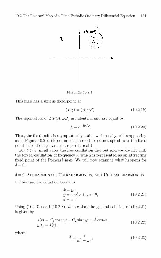
10.2 The Poincare Map of a Time-Periodic Ordinary Differential Equation 131
FIGURE 10.2.1.
This map has a unique fixed point at
(x, y) = (A, ωB). (10.2.19)
The eigenvalues of DP (A, ωB) are identical and are equal to
λ = e−δπ/ω. (10.2.20)
Thus, the fixed point is asymptotically stable with nearby orbits appearingas in Figure 10.2.2. (Note: in this case orbits do not spiral near the fixedpoint since the eigenvalues are purely real.)
For δ > 0, in all cases the free oscillation dies out and we are left withthe forced oscillation of frequency ω which is represented as an attractingfixed point of the Poincare map. We will now examine what happens forδ = 0.
δ = 0: Subharmonics, Ultraharmonics, and Ultrasubharmonics
In this case the equation becomes
x = y,y = −ω2
0x + γ cos θ,θ = ω.
(10.2.21)
Using (10.2.7c) and (10.2.8), we see that the general solution of (10.2.21)is given by
x(t) = C1 cos ω0t + C2 sinω0t + A cos ωt,y(t) = x(t),
(10.2.22)
whereA ≡ γ
ω20 − ω2 , (10.2.23)
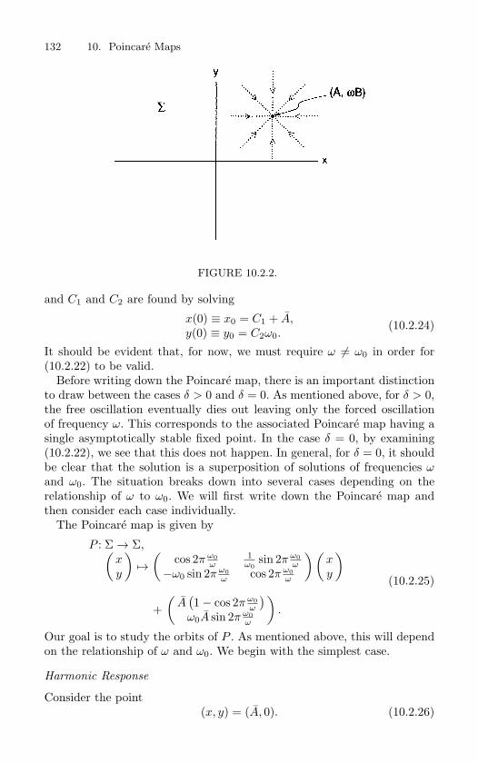
132 10. Poincare Maps
FIGURE 10.2.2.
and C1 and C2 are found by solving
x(0) ≡ x0 = C1 + A,y(0) ≡ y0 = C2ω0.
(10.2.24)
It should be evident that, for now, we must require ω = ω0 in order for(10.2.22) to be valid.
Before writing down the Poincare map, there is an important distinctionto draw between the cases δ > 0 and δ = 0. As mentioned above, for δ > 0,the free oscillation eventually dies out leaving only the forced oscillationof frequency ω. This corresponds to the associated Poincare map having asingle asymptotically stable fixed point. In the case δ = 0, by examining(10.2.22), we see that this does not happen. In general, for δ = 0, it shouldbe clear that the solution is a superposition of solutions of frequencies ωand ω0. The situation breaks down into several cases depending on therelationship of ω to ω0. We will first write down the Poincare map andthen consider each case individually.
The Poincare map is given by
P : Σ → Σ,(xy
)→
(cos 2π ω0
ω1
ω0sin 2π ω0
ω−ω0 sin 2π ω0
ω cos 2π ω0ω
)(xy
)
+(
A(1− cos 2π ω0
ω
)ω0A sin 2π ω0
ω
).
(10.2.25)
Our goal is to study the orbits of P . As mentioned above, this will dependon the relationship of ω and ω0. We begin with the simplest case.
Harmonic Response
Consider the point(x, y) = (A, 0). (10.2.26)
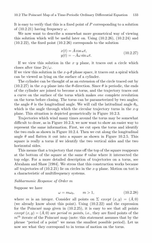
10.2 The Poincare Map of a Time-Periodic Ordinary Differential Equation 133
It is easy to verify that this is a fixed point of P corresponding to a solutionof (10.2.21) having frequency ω.
We now want to describe a somewhat more geometrical way of viewingthis solution which will be useful later on. Using (10.2.26), (10.2.24) and(10.2.22), the fixed point (10.2.26) corresponds to the solution
x(t) = A cos ωt,y(t) = −Aω sinωt.
(10.2.27)
If we view this solution in the x–y plane, it traces out a circle whichcloses after time 2π/ω.If we view this solution in the x-y-θ phase space, it traces out a spiral whichcan be viewed as lying on the surface of a cylinder.
The cylinder can be thought of as an extension of the circle traced out by(10.2.27) in the x-y plane into the θ-direction. Since θ is periodic, the endsof the cylinder are joined to become a torus, and the trajectory traces outa curve on the surface of the torus which makes one complete revolutionon the torus before closing. The torus can be parameterized by two angles;the angle θ is the longitudinal angle. We will call the latitudinal angle θ0,which is the angle through which the circular trajectory turns in the x-yplane. This situation is depicted geometrically in Figure 10.2.3.
Trajectories which wind many times around the torus may be somewhatdifficult to draw, as in Figure 10.2.3; we now want to show an easier way torepresent the same information. First, we cut open the torus and identifythe two ends as shown in Figure 10.2.4. Then we cut along the longitudinalangle θ and flatten it out into a square as shown in Figure 10.2.5. Thissquare is really a torus if we identify the two vertical sides and the twohorizontal sides.
This means that a trajectory that runs off the top of the square reappearsat the bottom of the square at the same θ value where it intersected thetop edge. For a more detailed description of trajectories on a torus, seeAbraham and Shaw [1984]. We stress that this construction works becauseall trajectories of (10.2.21) lie on circles in the x-y plane. Motion on tori isa characteristic of multifrequency systems.
Subharmonic Response of Order m
Suppose we haveω = mω0, m > 1, (10.2.28)
where m is an integer. Consider all points on Σ except (x, y) = (A, 0)(we already know about this point). Using (10.2.22) and the expressionfor the Poincare map given in (10.2.25), it is easy to see that all pointsexcept (x, y) = (A, 0) are period m points, i.e., they are fixed points of themth iterate of the Poincare map (note: this statement assumes that by thephrase “period of a point” we mean the smallest possible period). Let usnow see what they correspond to in terms of motion on the torus.
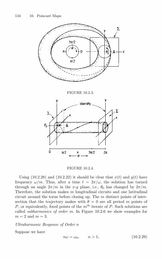
134 10. Poincare Maps
FIGURE 10.2.3.
FIGURE 10.2.4.
Using (10.2.28) and (10.2.22) it should be clear that x(t) and y(t) havefrequency ω/m. Thus, after a time t = 2π/ω, the solution has turnedthrough an angle 2π/m in the x-y plane, i.e., θ0 has changed by 2π/m.Therefore, the solution makes m longitudinal circuits and one latitudinalcircuit around the torus before closing up. The m distinct points of inter-section that the trajectory makes with θ = 0 are all period m points ofP , or equivalently, fixed points of the mth iterate of P . Such solutions arecalled subharmonics of order m. In Figure 10.2.6 we show examples form = 2 and m = 3.
Ultraharmonic Response of Order n
Suppose we havenω = ω0, n > 1, (10.2.29)
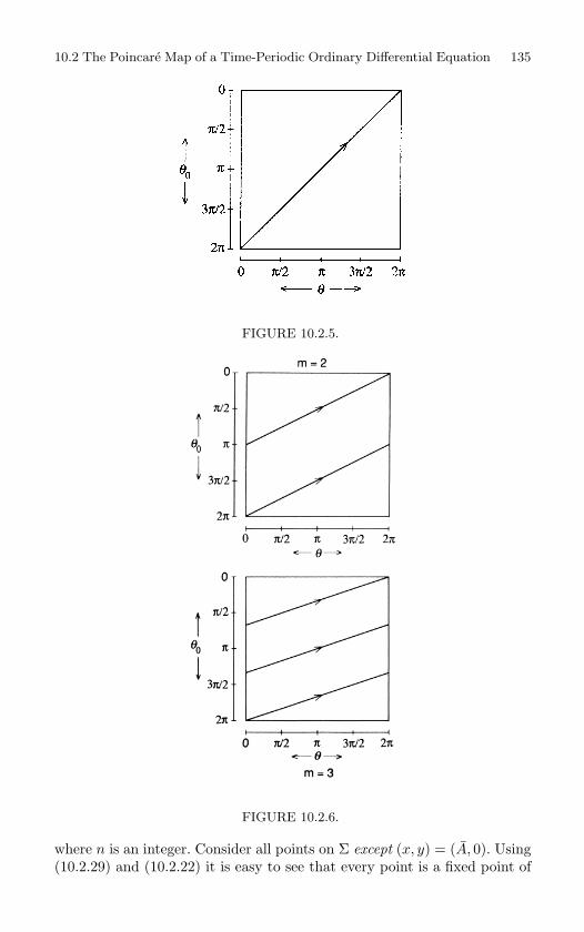
10.2 The Poincare Map of a Time-Periodic Ordinary Differential Equation 135
FIGURE 10.2.5.
FIGURE 10.2.6.
where n is an integer. Consider all points on Σ except (x, y) = (A, 0). Using(10.2.29) and (10.2.22) it is easy to see that every point is a fixed point of
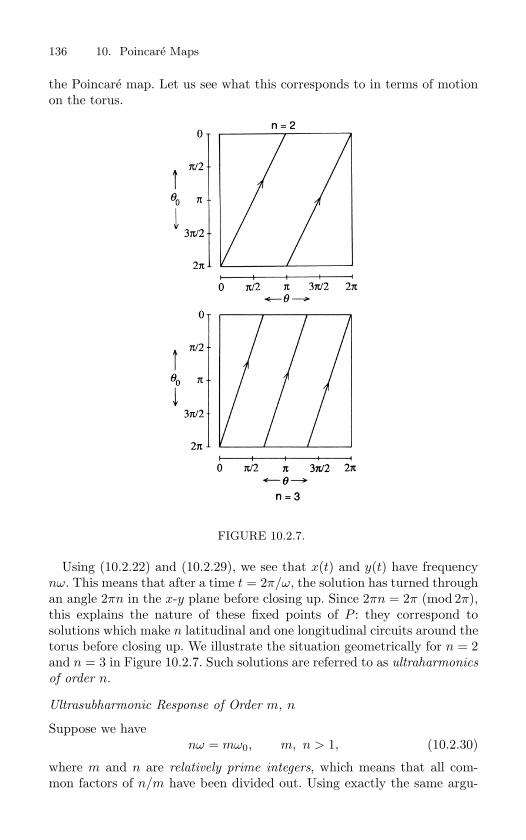
136 10. Poincare Maps
the Poincare map. Let us see what this corresponds to in terms of motionon the torus.
FIGURE 10.2.7.
Using (10.2.22) and (10.2.29), we see that x(t) and y(t) have frequencynω. This means that after a time t = 2π/ω, the solution has turned throughan angle 2πn in the x-y plane before closing up. Since 2πn = 2π (mod 2π),this explains the nature of these fixed points of P : they correspond tosolutions which make n latitudinal and one longitudinal circuits around thetorus before closing up. We illustrate the situation geometrically for n = 2and n = 3 in Figure 10.2.7. Such solutions are referred to as ultraharmonics
of order n.
Ultrasubharmonic Response of Order m, n
Suppose we havenω = mω0, m, n > 1, (10.2.30)
where m and n are relatively prime integers, which means that all com-mon factors of n/m have been divided out. Using exactly the same argu-
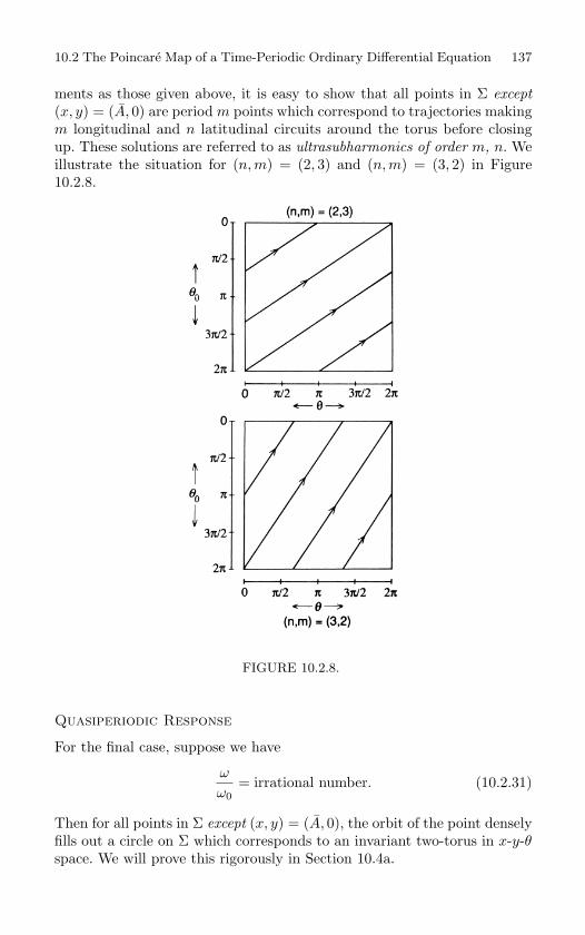
10.2 The Poincare Map of a Time-Periodic Ordinary Differential Equation 137
ments as those given above, it is easy to show that all points in Σ except
(x, y) = (A, 0) are period m points which correspond to trajectories makingm longitudinal and n latitudinal circuits around the torus before closingup. These solutions are referred to as ultrasubharmonics of order m, n. Weillustrate the situation for (n, m) = (2, 3) and (n, m) = (3, 2) in Figure10.2.8.
FIGURE 10.2.8.
Quasiperiodic Response
For the final case, suppose we have
ω
ω0= irrational number. (10.2.31)
Then for all points in Σ except (x, y) = (A, 0), the orbit of the point denselyfills out a circle on Σ which corresponds to an invariant two-torus in x-y-θspace. We will prove this rigorously in Section 10.4a.
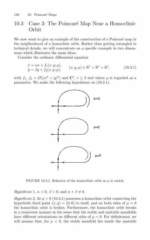
138 10. Poincare Maps
10.3 Case 3: The Poincare Map Near a HomoclinicOrbit
We now want to give an example of the construction of a Poincare map inthe neighborhood of a homoclinic orbit. Rather than getting entangled intechnical details, we will concentrate on a specific example in two dimen-sions which illustrates the main ideas.
Consider the ordinary differential equation
x = αx + f1(x, y; µ),y = βy + f2(x, y; µ), (x, y, µ) ∈ R
1 × R1 × R
1, (10.3.1)
with f1, f2 = O(|x|2 + |y|2) and Cr, r ≥ 2 and where µ is regarded as aparameter. We make the following hypotheses on (10.3.1).
FIGURE 10.3.1. Behavior of the homoclinic orbit as µ is varied.
Hypothesis 1. α < 0, β > 0, and α + β = 0.
Hypothesis 2. At µ = 0 (10.3.1) possesses a homoclinic orbit connecting thehyperbolic fixed point (x, y) = (0, 0) to itself, and on both sides of µ = 0the homoclinic orbit is broken. Furthermore, the homoclinic orbit breaksin a transverse manner in the sense that the stable and unstable manifoldshave different orientations on different sides of µ = 0. For definiteness, wewill assume that, for µ < 0, the stable manifold lies inside the unstable
10.3 The Poincare Map Near a Homoclinic Orbit 139
manifold, for µ > 0, the stable manifold lies outside the stable manifoldand, for µ = 0, they coincide; see Figure 10.3.1.
Hypothesis 1 is of a local nature, since it concerns the nature of theeigenvalues of the vector field linearized about the fixed point. Hypothesis2 is global in nature, since it supposes the existence of a homoclinic orbitand describes the nature of the parameter dependence of the homoclinicorbit.
Now an obvious question is why this scenario? Why not stable insidefor µ > 0 and unstable inside for µ < 0? Certainly this could happen;however, this is not important for us to consider at the moment. We needto know only that, on one side of µ = 0, the stable manifold lies inside theunstable manifold, and on the other side of µ = 0, the unstable manifoldlies inside the stable manifold. Of course, in applications, we would want todetermine which case actually occurs, and later on we will learn a methodfor doing this (Melnikov’s method); however, now we will simply study theconsequences of a homoclinic orbit to a hyperbolic fixed point of a planarvector field breaking in the manner described above.
Let us remark that it is certainly possible for the eigenvalues α and βto depend on the parameter µ. However, this will be of no consequenceprovided that Hypothesis 1 is satisfied for each parameter value and thatthis is true for µ sufficiently close to zero.
The question we ask is the following: What is the nature of the orbit
structure near the homoclinic orbit for µ near µ = 0? We will answerthis question by computing a Poincare map near the homoclinic orbit andstudying the orbit structure of the Poincare map. The Poincare map thatwe construct will be very different from those we constructed in Cases 1and 2 in that it will be the composition of two maps. One of the maps, P0,will be constructed from the flow near the origin (which we will take to bethe flow generated by the linearization of (10.3.1) about the origin). Theother map, P1, will be constructed from the flow outside of a neighbor-hood of the fixed point, which, if we remain close enough to the homoclinicorbit, can be made to be as close to a rigid motion as we like. The result-ing Poincare map, P , will then be given by P ≡ P1 P0. Evidently, withthese approximations, our Poincare map will be valid (meaning that its dy-namics reflect the dynamics of (10.3.1)) only when it is defined sufficientlyclose to the (broken) homoclinic orbit. We will discuss the validity of ourapproximations later on, but for now we begin our analysis.
The analysis will proceed in several steps.
Step 1. Set up the domain for the Poincare map.
Step 2. Compute P0.
Step 3. Compute P1.
Step 4. Examine the dynamics of P = P1 P0.
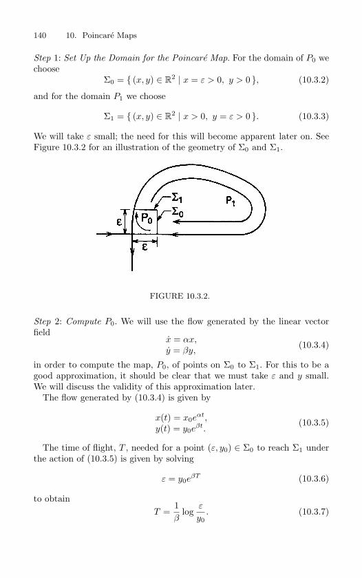
140 10. Poincare Maps
Step 1: Set Up the Domain for the Poincare Map. For the domain of P0 wechoose
Σ0 = (x, y) ∈ R2 | x = ε > 0, y > 0 , (10.3.2)
and for the domain P1 we choose
Σ1 = (x, y) ∈ R2 | x > 0, y = ε > 0 . (10.3.3)
We will take ε small; the need for this will become apparent later on. SeeFigure 10.3.2 for an illustration of the geometry of Σ0 and Σ1.
FIGURE 10.3.2.
Step 2: Compute P0. We will use the flow generated by the linear vectorfield
x = αx,y = βy,
(10.3.4)
in order to compute the map, P0, of points on Σ0 to Σ1. For this to be agood approximation, it should be clear that we must take ε and y small.We will discuss the validity of this approximation later.
The flow generated by (10.3.4) is given by
x(t) = x0eαt,
y(t) = y0eβt.
(10.3.5)
The time of flight, T , needed for a point (ε, y0) ∈ Σ0 to reach Σ1 underthe action of (10.3.5) is given by solving
ε = y0eβT (10.3.6)
to obtainT =
1β
logε
y0. (10.3.7)
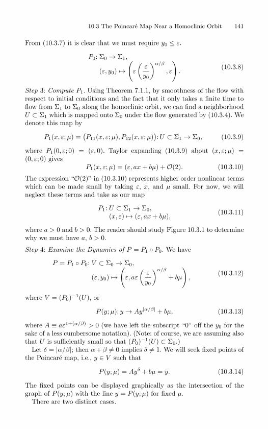
10.3 The Poincare Map Near a Homoclinic Orbit 141
From (10.3.7) it is clear that we must require y0 ≤ ε.
P0: Σ0 → Σ1,
(ε, y0) →(
ε
(ε
y0
)α/β
, ε
).
(10.3.8)
Step 3: Compute P1. Using Theorem 7.1.1, by smoothness of the flow withrespect to initial conditions and the fact that it only takes a finite time toflow from Σ1 to Σ0 along the homoclinic orbit, we can find a neighborhoodU ⊂ Σ1 which is mapped onto Σ0 under the flow generated by (10.3.4). Wedenote this map by
P1(x, ε; µ) =(P11(x, ε;µ), P12(x, ε;µ)
):U ⊂ Σ1 → Σ0, (10.3.9)
where P1(0, ε; 0) = (ε, 0). Taylor expanding (10.3.9) about (x, ε;µ) =(0, ε; 0) gives
P1(x, ε;µ) = (ε, ax + bµ) +O(2). (10.3.10)
The expression “O(2)” in (10.3.10) represents higher order nonlinear termswhich can be made small by taking ε, x, and µ small. For now, we willneglect these terms and take as our map
P1: U ⊂ Σ1 → Σ0,(x, ε) → (ε, ax + bµ), (10.3.11)
where a > 0 and b > 0. The reader should study Figure 10.3.1 to determinewhy we must have a, b > 0.
Step 4: Examine the Dynamics of P = P1 P0. We have
P = P1 P0: V ⊂ Σ0 → Σ0,
(ε, y0) →(
ε, aε
(ε
y0
)α/β
+ bµ
),
(10.3.12)
where V = (P0)−1(U), or
P (y;µ): y → Ay|α/β| + bµ, (10.3.13)
where A ≡ aε1+(α/β) > 0 (we have left the subscript “0” off the y0 for thesake of a less cumbersome notation). (Note: of course, we are assuming alsothat U is sufficiently small so that (P0)−1(U) ⊂ Σ0.)
Let δ = |α/β|; then α + β = 0 implies δ = 1. We will seek fixed points ofthe Poincare map, i.e., y ∈ V such that
P (y; µ) = Ayδ + bµ = y. (10.3.14)
The fixed points can be displayed graphically as the intersection of thegraph of P (y; µ) with the line y = P (y;µ) for fixed µ.
There are two distinct cases.
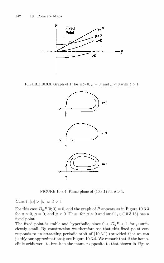
142 10. Poincare Maps
FIGURE 10.3.3. Graph of P for µ > 0, µ = 0, and µ < 0 with δ > 1.
FIGURE 10.3.4. Phase plane of (10.3.1) for δ > 1.
Case 1: |α| > |β| or δ > 1
For this case DyP (0; 0) = 0, and the graph of P appears as in Figure 10.3.3for µ > 0, µ = 0, and µ < 0. Thus, for µ > 0 and small µ, (10.3.13) has afixed point.The fixed point is stable and hyperbolic, since 0 < DyP < 1 for µ suffi-ciently small. By construction we therefore see that this fixed point cor-responds to an attracting periodic orbit of (10.3.1) (provided that we canjustify our approximations); see Figure 10.3.4. We remark that if the homo-clinic orbit were to break in the manner opposite to that shown in Figure
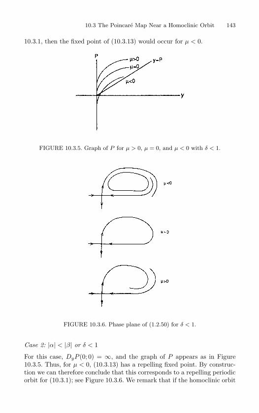
10.3 The Poincare Map Near a Homoclinic Orbit 143
10.3.1, then the fixed point of (10.3.13) would occur for µ < 0.
FIGURE 10.3.5. Graph of P for µ > 0, µ = 0, and µ < 0 with δ < 1.
FIGURE 10.3.6. Phase plane of (1.2.50) for δ < 1.
Case 2: |α| < |β| or δ < 1
For this case, DyP (0; 0) = ∞, and the graph of P appears as in Figure10.3.5. Thus, for µ < 0, (10.3.13) has a repelling fixed point. By construc-tion we can therefore conclude that this corresponds to a repelling periodicorbit for (10.3.1); see Figure 10.3.6. We remark that if the homoclinic orbit
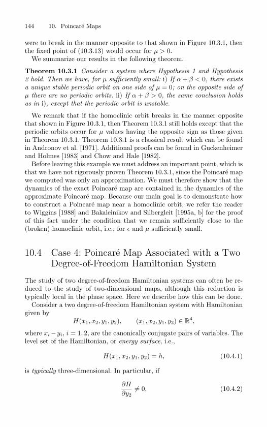
144 10. Poincare Maps
were to break in the manner opposite to that shown in Figure 10.3.1, thenthe fixed point of (10.3.13) would occur for µ > 0.
We summarize our results in the following theorem.
Theorem 10.3.1 Consider a system where Hypothesis 1 and Hypothesis
2 hold. Then we have, for µ sufficiently small: i) If α + β < 0, there exists
a unique stable periodic orbit on one side of µ = 0; on the opposite side of
µ there are no periodic orbits. ii) If α + β > 0, the same conclusion holds
as in i), except that the periodic orbit is unstable.
We remark that if the homoclinic orbit breaks in the manner oppositethat shown in Figure 10.3.1, then Theorem 10.3.1 still holds except that theperiodic orbits occur for µ values having the opposite sign as those givenin Theorem 10.3.1. Theorem 10.3.1 is a classical result which can be foundin Andronov et al. [1971]. Additional proofs can be found in Guckenheimerand Holmes [1983] and Chow and Hale [1982].
Before leaving this example we must address an important point, which isthat we have not rigorously proven Theorem 10.3.1, since the Poincare mapwe computed was only an approximation. We must therefore show that thedynamics of the exact Poincare map are contained in the dynamics of theapproximate Poincare map. Because our main goal is to demonstrate howto construct a Poincare map near a homoclinic orbit, we refer the readerto Wiggins [1988] and Bakaleinikov and Silbergleit [1995a, b] for the proofof this fact under the condition that we remain sufficiently close to the(broken) homoclinic orbit, i.e., for ε and µ sufficiently small.
10.4 Case 4: Poincare Map Associated with a TwoDegree-of-Freedom Hamiltonian System
The study of two degree-of-freedom Hamiltonian systems can often be re-duced to the study of two-dimensional maps, although this reduction istypically local in the phase space. Here we describe how this can be done.
Consider a two degree-of-freedom Hamiltonian system with Hamiltoniangiven by
H(x1, x2, y1, y2), (x1, x2, y1, y2) ∈ R4,
where xi−yi, i = 1, 2, are the canonically conjugate pairs of variables. Thelevel set of the Hamiltonian, or energy surface, i.e.,
H(x1, x2, y1, y2) = h, (10.4.1)
is typically three-dimensional. In particular, if
∂H
∂y2 = 0, (10.4.2)
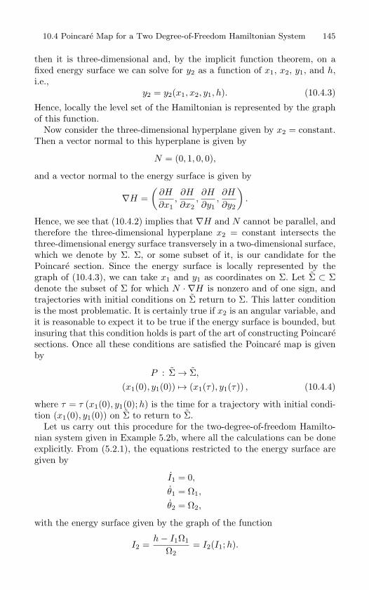
10.4 Poincare Map for a Two Degree-of-Freedom Hamiltonian System 145
then it is three-dimensional and, by the implicit function theorem, on afixed energy surface we can solve for y2 as a function of x1, x2, y1, and h,i.e.,
y2 = y2(x1, x2, y1, h). (10.4.3)
Hence, locally the level set of the Hamiltonian is represented by the graphof this function.
Now consider the three-dimensional hyperplane given by x2 = constant.Then a vector normal to this hyperplane is given by
N = (0, 1, 0, 0),
and a vector normal to the energy surface is given by
∇H =(
∂H
∂x1,∂H
∂x2,∂H
∂y1,∂H
∂y2
).
Hence, we see that (10.4.2) implies that ∇H and N cannot be parallel, andtherefore the three-dimensional hyperplane x2 = constant intersects thethree-dimensional energy surface transversely in a two-dimensional surface,which we denote by Σ. Σ, or some subset of it, is our candidate for thePoincare section. Since the energy surface is locally represented by thegraph of (10.4.3), we can take x1 and y1 as coordinates on Σ. Let Σ ⊂ Σdenote the subset of Σ for which N · ∇H is nonzero and of one sign, andtrajectories with initial conditions on Σ return to Σ. This latter conditionis the most problematic. It is certainly true if x2 is an angular variable, andit is reasonable to expect it to be true if the energy surface is bounded, butinsuring that this condition holds is part of the art of constructing Poincaresections. Once all these conditions are satisfied the Poincare map is givenby
P : Σ→ Σ,
(x1(0), y1(0)) → (x1(τ), y1(τ)) , (10.4.4)
where τ = τ (x1(0), y1(0);h) is the time for a trajectory with initial condi-tion (x1(0), y1(0)) on Σ to return to Σ.
Let us carry out this procedure for the two-degree-of-freedom Hamilto-nian system given in Example 5.2b, where all the calculations can be doneexplicitly. From (5.2.1), the equations restricted to the energy surface aregiven by
I1 = 0,
θ1 = Ω1,
θ2 = Ω2,
with the energy surface given by the graph of the function
I2 =h− I1Ω1
Ω2= I2(I1;h).
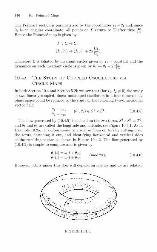
146 10. Poincare Maps
The Poincare section is parametrized by the coordinates I1− θ1 and, sinceθ2 is an angular coordinate, all points on Σ return to Σ after time 2π
Ω2.
Hence the Poincare map is given by
P : Σ→ Σ,
(I1, θ1) → (I1, θ1 + 2πΩ1
Ω2).
Therefore Σ is foliated by invariant circles given by I1 = constant and thedynamics on each invariant circle is given by θ1 → θ1 + 2π Ω1
Ω2.
10.4a The Study of Coupled Oscillators viaCircle Maps
In both Section 10.4 and Section 5.2b we saw that (for I1, I2 = 0) the studyof two linearly coupled, linear undamped oscillators in a four-dimensionalphase space could be reduced to the study of the following two-dimensionalvector field
θ1 = ω1,θ2 = ω2,
(θ1, θ2) ∈ S1 × S1. (10.4.5)
The flow generated by (10.4.5) is defined on the two-torus, S1×S1 ≡ T 2,and θ1 and θ2 are called the longitude and latitude; see Figure 10.4.1. As inExample 10.2a, it is often easier to visualize flows on tori by cutting openthe torus, flattening it out, and identifying horizontal and vertical sidesof the resulting square as shown in Figure 10.4.2. The flow generated by(10.4.5) is simple to compute and is given by
θ1(t) = ω1t + θ10,θ2(t) = ω2t + θ20,
(mod 2π). (10.4.6)
However, orbits under this flow will depend on how ω1 and ω2 are related.
FIGURE 10.4.1.
10.4 Poincare Map for a Two Degree-of-Freedom Hamiltonian System 147
FIGURE 10.4.2.
Definition 10.4.1 ω1 and ω2 are said to be incommensurate if the equa-
tion
mω1 + nω2 = 0
has no solutions consisting of n, m ∈ Z (integers). Otherwise, ω1 and ω2are commensurate.
Theorem 10.4.2 If ω1 and ω2 are commensurate, then every phase curve
of (10.4.5) is closed. However, if ω1 and ω2 are incommensurate, then every
phase curve of (10.4.5) is everywhere dense on the torus.
To prove this theorem, we need the following lemma.
Lemma 10.4.3 Suppose the circle S1 is rotated through an angle α, and
α is incommensurate with 2π. Then the sequence
S = θ, θ + α, θ + 2α, · · · , θ + nα, · · · , (mod 2π)
is everywhere dense on the circle (note: n is an integer).
Proof:
θ + mα(mod 2π) =
θ + mα if mα− 2π < 0,θ + (mα− 2πk) if mα− 2πk > 0, k > 1
and mα− 2π(k + 1) < 0,
so, in particular, since α and 2π are incommensurate, the sequence S isinfinite and never repeats.
We will use the “pigeonhole principle,” i.e., if you have n holes and n+1pigeons, then one hole must contain at least two pigeons.
Divide the circle into k half-open intervals of equal length 2π/k. Then,among the first k + 1 elements of the sequence S, at least two must be inthe same half-open interval; call these points θ + pα, θ + qα(mod 2π) with
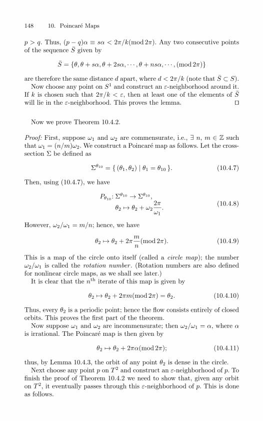
148 10. Poincare Maps
p > q. Thus, (p − q)α ≡ sα < 2π/k(mod 2π). Any two consecutive pointsof the sequence S given by
S = θ, θ + sα, θ + 2sα, · · · , θ + nsα, · · · , (mod 2π)
are therefore the same distance d apart, where d < 2π/k (note that S ⊂ S).Now choose any point on S1 and construct an ε-neighborhood around it.
If k is chosen such that 2π/k < ε, then at least one of the elements of Swill lie in the ε-neighborhood. This proves the lemma.
Now we prove Theorem 10.4.2.
Proof: First, suppose ω1 and ω2 are commensurate, i.e., ∃ n, m ∈ Z suchthat ω1 = (n/m)ω2. We construct a Poincare map as follows. Let the cross-section Σ be defined as
Σθ10 = (θ1, θ2) | θ1 = θ10 . (10.4.7)
Then, using (10.4.7), we have
Pθ10 : Σθ10 → Σθ10 ,
θ2 → θ2 + ω22π
ω1.
(10.4.8)
However, ω2/ω1 = m/n; hence, we have
θ2 → θ2 + 2πm
n(mod 2π). (10.4.9)
This is a map of the circle onto itself (called a circle map); the numberω2/ω1 is called the rotation number . (Rotation numbers are also definedfor nonlinear circle maps, as we shall see later.)
It is clear that the nth iterate of this map is given by
θ2 → θ2 + 2πm(mod 2π) = θ2. (10.4.10)
Thus, every θ2 is a periodic point; hence the flow consists entirely of closedorbits. This proves the first part of the theorem.
Now suppose ω1 and ω2 are incommensurate; then ω2/ω1 = α, where αis irrational. The Poincare map is then given by
θ2 → θ2 + 2πα(mod 2π); (10.4.11)
thus, by Lemma 10.4.3, the orbit of any point θ2 is dense in the circle.Next choose any point p on T 2 and construct an ε-neighborhood of p. To
finish the proof of Theorem 10.4.2 we need to show that, given any orbiton T 2, it eventually passes through this ε-neighborhood of p. This is doneas follows.
10.5 Exercises 149
First, we are able to construct a new cross-section Σθ10 which passesthrough the ε-neighborhood of p; see Figure 10.4.3. We have seen that theorbits of Pθ10 : Σ
θ10 → Σθ10 are all dense on Σθ10 for any θ10. Therefore, wecan take any point on Σθ10 and look at its first intersection point with Σθ10
under the flow (10.4.6). From this it follows that the iterates of this pointunder Pθ10
are dense in Σθ10 . This completes the proof.
FIGURE 10.4.3.
Let us make a final remark before leaving this example. In our intro-ductory motivational remarks we stated that Poincare maps allow a di-mensional reduction of the problem by at least one. In this example, wehave seen how the study of a four-dimensional system can be reduced tothe study of a one-dimensional system. This was possible because of ourunderstanding of the geometry of the phase space; i.e., the phase space wasmade up of families of two-tori. It will be a common theme throughout thisbook that a good qualitative feel for the geometry of the phase space willput us in the best position for quantitative analysis.
Finally, we note that these results for linear vector fields on T 2 actuallyremain true for nonlinear differentiable vector fields on T 2, namely, thatthe ω limit sets for vector fields with no singular points are either closedorbits or the entire torus; see Hale [1980].
10.5 ExercisesExercises 1 − 3 are concerned with the properties of the following Poincare map.
Consider the Poincare map given in (10.2.15)
(xy
)→ e
−δπ/ω
C + δ2ω S 1
ω S
− ω20
ω S C − δ2ω S
(
xy
)
150 10. Poincare Maps
+
e−δπ/ω [−AC + ( −δ
2ω A − ωω B)S] + A
e−δπ/ω [−ωBC + (ω20
ω A + δω2ω B)S] + ωB
,
whereC = cos 2π
ω
ω, S = sin 2π
ω
ω,
and
ω =12
√4ω2
0 − δ2, A =(ω2
0 − ω2)γ(ω2
0 − ω2)2 + (δω)2, B =
δγω
(ω20 − ω2)2 + (δω)2
.
1. Show that (x, y) = (A, ωB) is the only fixed point for this map and, hence, argue that itis a global attractor.
2. Discuss the nature of the orbit structure near (x, y) = (A, ωB) for different values of ω/ω.
3. Show how the fixed point of the Poincare map changes as the cross-section (i.e., phaseangle) is varied.
4. Construct and study the Poincare map for
x = y,
y = −ω20x + γ cos θ,
θ = ω0.
Exercises 5 − 9 are concerned with the properties of the following Poincare map.Consider the Poincare map (ω = ω0) given in (10.2.25)
(xy
)→
(cos 2π
ω0ω
1ω0
sin 2πω0ω
−ω0 sin 2πω0ω cos 2π
ω0ω
)(xy
)
+(
A(1 − cos 2πω0ω )
ω0A sin 2πω0ω
).
5. For ω = mω0, m > 1, show that all points except (x, y) = (A, 0) are period m points.
6. For nω = ω0, n > 1, show that all points are fixed points.
7. Discuss the orbit structure of the Poincare map when ω/ω0 is an irrational number.
8. Discuss stability of the harmonics, subharmonics, ultraharmonics, and ultrasubharmonics.
9. Recall that a C1 map, f , preserves orientation when det Df > 0. Show that the four typesof Poincare maps discussed in this section preserve orientation. What would be theconsequences if they did not?
10. Consider an n degree-of-freedom Hamiltonian system. Following the discussion in Section10.4, discuss how it can be studied via a 2n − 2 dimensional Poincare map.
11. Show that the Poincare maps for Hamiltonian systems described in Section 10.4 andExercise 10 preserve volume.
11
Conjugacies of Maps, andVarying the Cross-Section
We now turn to answering the question of how the choice of cross-sectionaffects the Poincare map. The point of view that we develop will be thatPoincare maps defined on different cross-sections are related by a (in gen-eral, nonlinear) coordinate transformation. The importance of coordinatetransformations in the study of dynamical systems cannot be overesti-mated. For example, in the study of systems of linear constant coefficientordinary differential equations, coordinate transformations allow one to de-couple the system and hence reduce the system to a set of decoupled linearfirst-order equations which are easily solved. In the study of completelyintegrable Hamiltonian systems, the transformations to action-angle coor-dinates results in a trivially solvable system (see Arnold [1978]), and thesecoordinates are also useful in the study of near integrable systems. If weconsider general properties of dynamical systems, coordinate transforma-tions provide us with a way of classifying dynamical systems according toproperties which remain unchanged after a coordinate transformation. InChapter 12 we will see that the notion of structural stability is based onsuch a classification scheme.
Before considering Poincare maps, we want to discuss coordinate trans-formations, or, to use the more general mathematical term, conjugacies,
giving some results that describe properties which must be retained by amap or vector field after a coordinate transformation of a specific differen-tiability class. Let us begin with an example which should be familiar tothe reader.
Example 11.0.1. We want to motivate how coordinate transformations affect
the orbits of maps.
Consider two linear, invertible maps
x → Ax, x ∈ Rn
(11.0.1)
y → By, y ∈ Rn. (11.0.2)
For x0 ∈ Rn, we denote the orbit of x0 under A by
OA(x0) = · · · , A−nx0, · · · , A−1x0, x0, Ax0, · · · , Anx0, · · ·, (11.0.3)
and, for y0 ∈ Rn, we denote the orbit of y0 under B by
152 11. Conjugacies of Maps, and Varying the Cross-Section
OB(y0) = · · · , B−ny0, · · · , B−1y0, y0, By0, · · · , Bny0, · · ·. (11.0.4)
Now suppose A and B are related by a similarity transformation, i.e., there is an
invertible matrix T such that
B = TAT −1. (11.0.5)
We could think of T as transforming A into B, and, hence, since it does no harm
in the linear setting to confuse the map with the matrix that generates it, Ttransforms (11.0.1) into (11.0.2). We represent this in the following diagram
Rn A−→ RnT
T
Rn B−→ Rn
. (11.0.6)
The question we want to answer is this: when (11.0.1) is transformed into (11.0.2)
via (11.0.5), how are orbits of A related to orbits of B? To answer this question,
note that from (11.0.5) we have
Bn= TAnT −1
for all n. (11.0.7)
Hence, using (11.0.7) and comparing (11.0.1) and (11.0.5), we see that orbits of
A are mapped to orbits of B under the transformation y = Tx. Moreover, we
know that since similar matrices have the same eigenvalues, the stability types
of these orbits coincide under the transformation T .
End of Example 11.0.1
Now we want to consider coordinate transformation in a more general,nonlinear setting. However, the reader will see that the essence of the ideasis contained in this example.
Let us consider two Cr diffeomorphisms f : Rn → Rn and g: Rn → R
n,and a Ck diffeomorphism h: Rn → R
n.
Definition 11.0.1 (Conjugacy) f and g are said to be Ck conjugate(k ≤ r) if there exists a Ck diffeomorphism h: Rn → R
n such that g h =h f . If k = 0, f and g are said to be topologically conjugate.
The conjugacy of two diffeomorphisms is often represented by the fol-lowing diagram.
Rn f−→ R
n&h
&h
Rn g−→ R
n
. (11.0.8)
The diagram is said to commute if the relation g h = hf holds, meaningthat you can start at a point in the upper left-hand corner of the diagramand reach the same point in the lower right-hand corner of the diagram byeither of the two possible routes. We note that h need not be defined on allof R
n but possibly only locally about a given point. In such cases, f and gare said to be locally Ck conjugate.
If f and g are Ck conjugate, then we have the following results.
11. Conjugacies of Maps, and Varying the Cross-Section 153
Proposition 11.0.2 If f and g are Ck conjugate, then orbits of f map to
orbits of g under h.
Proof: Let x0 ∈ Rn; then the orbit of x0 under f is given by
O(x0) = · · · , f−n(x0), · · · , f−1(x0), x0, f(x0), · · · , fn(x0), · · ·. (11.0.9)
From Definition 11.0.1, we have that f = h−1 g h, so for a given n > 0we have
fn(x0) = (h−1 g h) (h−1 g h) · · · (h−1 g h)︸ ︷︷ ︸n factors
(x0)
= h−1 gn h(x0) (11.0.10)
orh fn(x0) = gn h(x0). (11.0.11)
Also from Definition 1.2.2, we have that f−1 = h−1 g−1 h, so by thesame argument, for n > 0 we obtain
h f−n(x0) = g−n h(x0). (11.0.12)
Therefore, from (11.0.10) and (11.0.12) we see that the orbit of x0 under fis mapped by h to the orbit of h(x0) under g.
Proposition 11.0.3 If f and g are Ck conjugate, k ≥ 1, and x0 is a fixed
point of f , then the eigenvalues of Df(x0) are equal to the eigenvalues of
Dg(h(x0)
).
Proof: From Definition 11.0.1, f(x) = h−1 g h(x). Note that since x0 is afixed point then h−1 gh(x0) = x0. Also, by the inverse function theorem,we have Dh−1 = (Dh)−1. Using this and the fact that h is differentiable,we have
Df∣∣x0
= Dh−1∣∣x0
Dg∣∣h(x0)
Dh∣∣x0
. (11.0.13)
Therefore, recalling that similar matrices have equal eigenvalues gives theresult.
Now we will return to the specific question of what happens to thePoincare map when the cross-section is changed. We begin with Case 1,a Poincare map defined near a periodic orbit.
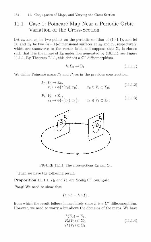
154 11. Conjugacies of Maps, and Varying the Cross-Section
11.1 Case 1: Poincare Map Near a Periodic Orbit:Variation of the Cross-Section
Let x0 and x1 be two points on the periodic solution of (10.1.1), and letΣ0 and Σ1 be two (n− 1)-dimensional surfaces at x0 and x1, respectively,which are transverse to the vector field, and suppose that Σ1 is chosensuch that it is the image of Σ0 under flow generated by (10.1.1); see Figure11.1.1. By Theorem 7.1.1, this defines a Cr diffeomorphism
h: Σ0 → Σ1. (11.1.1)
We define Poincare maps P0 and P1 as in the previous construction.
P0: V0 → Σ0,x0 → φ
(τ(x0), x0
), x0 ∈ V0 ⊂ Σ0,
(11.1.2)
P1: V1 → Σ1,x1 → φ
(τ(x1), x1
), x1 ∈ V1 ⊂ Σ1.
(11.1.3)
FIGURE 11.1.1. The cross-sections Σ0 and Σ1.
Then we have the following result.
Proposition 11.1.1 P0 and P1 are locally Cr conjugate.
Proof: We need to show that
P1 h = h P0,
from which the result follows immediately since h is a Cr diffeomorphism.However, we need to worry a bit about the domains of the maps. We have
h(Σ0) = Σ1,P0(V0) ⊂ Σ0,P1(V1) ⊂ Σ1.
(11.1.4)
11.2 Variation of the Cross-Section of the Poincare Map: Case 2 155
Thus, h P0:V0 → Σ1 is well defined but P1 h need not be defined, sinceP1 is not defined on all of Σ1; however, this problem is solved if we chooseΣ1 such that V1 = h(V0) and take V0 sufficiently small.
11.2 Case 2: The Poincare Map of a Time-PeriodicOrdinary Differential Equation: Variation ofthe Cross-Section
Consider the Poincare map Pθ0defined on the cross-section Σθ0 as defined
in (10.2.5). Suppose we construct a different Poincare map, Pθ1, in the same
manner but on the cross-section
Σθ1 =
(x, θ) ∈ Rn × S1 | θ = θ1 ∈ (0, 2π]
. (11.2.1)
Then we have the following result.
Proposition 11.2.1 Pθ0and Pθ1
are Cr conjugate.
Proof: The proof follows a construction similar to that given in Proposition11.1.1. We construct a Cr diffeomorphism, h, of Σθ0 into Σθ1 by mappingpoints on Σθ0 into Σθ1 under the action of the flow generated by (10.2.3).Points starting on Σθ0 have initial time t0 = (θ0 − θ0)/ω, and they reachΣθ1 after time
t =θ1 − θ0
ω;
thus we have
h: Σθ0 → Σθ1 ,(x
(θ0 − θ0
ω
), θ0
)→
(x
(θ1 − θ0
ω
), θ1
).
(11.2.2)
Using (11.2.2) and the expression for the Poincare maps defined on thedifferent cross-sections, we obtain
h Pθ0: Σθ0 → Σθ1 ,(
x
(θ0 − θ0
ω
), θ0
)→
(x
(θ1 − θ0 + 2π
ω
), θ1 + 2π ≡ θ1
),
(11.2.3)and
Pθ1 h: Σθ0 → Σθ1 ,(
x
(θ0 − θ0
ω
), θ0
)→
(x
(θ1 − θ0 + 2π
ω
), θ1 + 2π ≡ θ1
).
(11.2.4)
156 11. Conjugacies of Maps, and Varying the Cross-Section
Thus, from (11.2.3) and (11.2.4), we have that
h Pθ0= Pθ1
h. (11.2.5)
Therefore, Propositions 11.0.2 and 11.0.3 imply that, as long as we re-main sufficiently close to the periodic orbit, changing the cross-section doesnot have any dynamical effect in the sense that we will still have the sameorbits with the same stability type. However, geometrically there may bean apparent difference in the sense that the locations of the orbits as wellas their stable and unstable manifolds may “move around” under a changein cross-section. It may also be possible that an intelligent choice of thecross-section could result in a “more symmetric” Poincare map which couldfacilitate the analysis. We will see an example of this later.
We note that the case of a Poincare map near a homoclinic orbit can betreated in the same way with the same results. We leave this as an exercisefor the reader.
We remark that it should be clear from these results that a Poincaremap constructed according to Case 2 (i.e., the global cross-section) hasinformation concerning all possible dynamics of the vector field. When onlya local cross-section can be constructed, then the Poincare map will not,in general, contain information on all possible dynamics of the vector field.Different Poincare maps defined on different cross-sections may not havethe same dynamics.
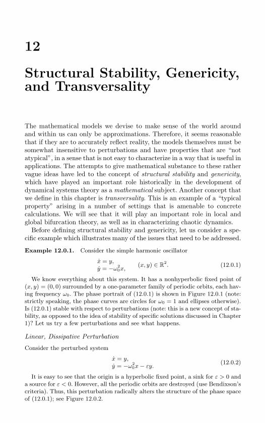
12
Structural Stability, Genericity,and Transversality
The mathematical models we devise to make sense of the world aroundand within us can only be approximations. Therefore, it seems reasonablethat if they are to accurately reflect reality, the models themselves must besomewhat insensitive to perturbations and have properties that are “notatypical”, in a sense that is not easy to characterize in a way that is useful inapplications. The attempts to give mathematical substance to these rathervague ideas have led to the concept of structural stability and genericity,which have played an important role historically in the development ofdynamical systems theory as a mathematical subject. Another concept thatwe define in this chapter is transversality. This is an example of a “typicalproperty” arising in a number of settings that is amenable to concretecalculations. We will see that it will play an important role in local andglobal bifurcation theory, as well as in characterizing chaotic dynamics.
Before defining structural stability and genericity, let us consider a spe-cific example which illustrates many of the issues that need to be addressed.
Example 12.0.1. Consider the simple harmonic oscillator
x = y,y = −ω2
0x,(x, y) ∈ R
2. (12.0.1)
We know everything about this system. It has a nonhyperbolic fixed point of
(x, y) = (0, 0) surrounded by a one-parameter family of periodic orbits, each hav-
ing frequency ω0. The phase portrait of (12.0.1) is shown in Figure 12.0.1 (note:
strictly speaking, the phase curves are circles for ω0 = 1 and ellipses otherwise).
Is (12.0.1) stable with respect to perturbations (note: this is a new concept of sta-
bility, as opposed to the idea of stability of specific solutions discussed in Chapter
1)? Let us try a few perturbations and see what happens.
Linear, Dissipative Perturbation
Consider the perturbed system
x = y,y = −ω2
0x − εy.(12.0.2)
It is easy to see that the origin is a hyperbolic fixed point, a sink for ε > 0 and
a source for ε < 0. However, all the periodic orbits are destroyed (use Bendixson’s
criteria). Thus, this perturbation radically alters the structure of the phase space
of (12.0.1); see Figure 12.0.2.
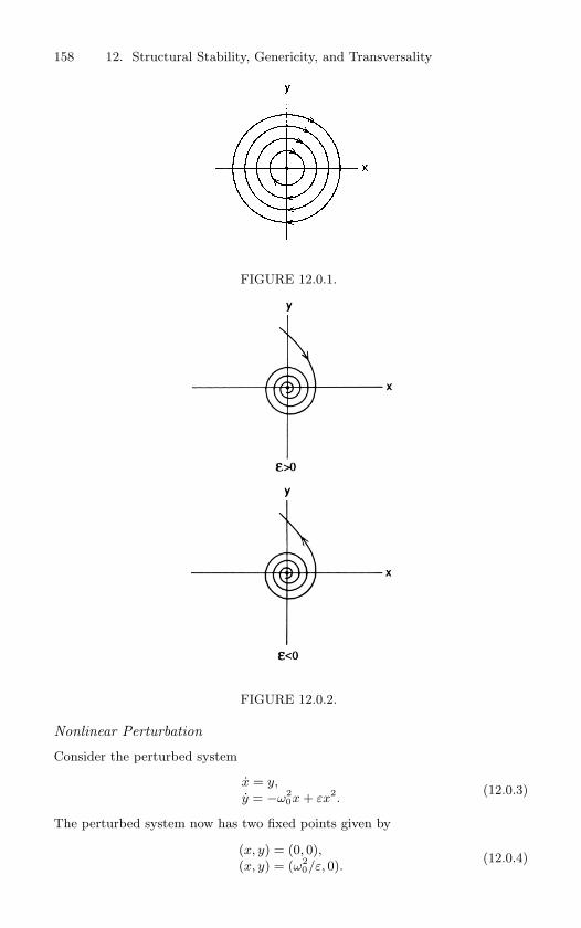
158 12. Structural Stability, Genericity, and Transversality
FIGURE 12.0.1.
FIGURE 12.0.2.
Nonlinear Perturbation
Consider the perturbed system
x = y,y = −ω2
0x + εx2.(12.0.3)
The perturbed system now has two fixed points given by
(x, y) = (0, 0),(x, y) = (ω2
0/ε, 0).(12.0.4)
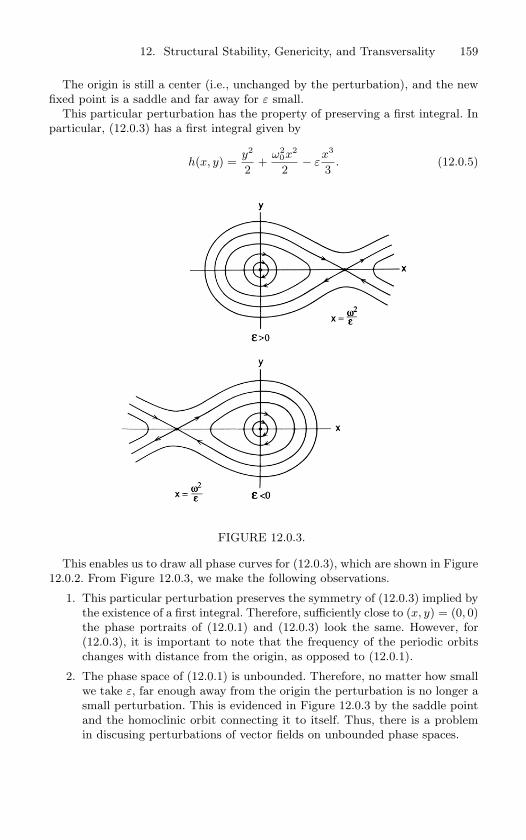
12. Structural Stability, Genericity, and Transversality 159
The origin is still a center (i.e., unchanged by the perturbation), and the new
fixed point is a saddle and far away for ε small.
This particular perturbation has the property of preserving a first integral. In
particular, (12.0.3) has a first integral given by
h(x, y) =y2
2+
ω20x2
2− ε
x3
3. (12.0.5)
FIGURE 12.0.3.
This enables us to draw all phase curves for (12.0.3), which are shown in Figure
12.0.2. From Figure 12.0.3, we make the following observations.
1. This particular perturbation preserves the symmetry of (12.0.3) implied by
the existence of a first integral. Therefore, sufficiently close to (x, y) = (0, 0)
the phase portraits of (12.0.1) and (12.0.3) look the same. However, for
(12.0.3), it is important to note that the frequency of the periodic orbits
changes with distance from the origin, as opposed to (12.0.1).
2. The phase space of (12.0.1) is unbounded. Therefore, no matter how small
we take ε, far enough away from the origin the perturbation is no longer a
small perturbation. This is evidenced in Figure 12.0.3 by the saddle point
and the homoclinic orbit connecting it to itself. Thus, there is a problem
in discusing perturbations of vector fields on unbounded phase spaces.
160 12. Structural Stability, Genericity, and Transversality
Time-Dependent Perturbation
Consider the systemx = y,y = −ω2
0x + εx cos t.(12.0.6)
This perturbation is of a very different character than the previous two. Writing
(12.0.6) as an autonomous system (see Chapter 7)
x = y,y = −ω2
0x + εx cos θ,θ = 1,
(12.0.7)
we see that the time-dependent perturbation has the effect of enlarging the di-
mension of the system. However, in any case, (x, y) = (0, 0) is still a fixed point
of (12.0.6), although it is interpreted as a periodic orbit of (12.0.7). We now ask
what the nature of the flow is near (x, y) = (0, 0), which is a difficult question
to answer due to the time dependence. Equation (12.0.6) is known as the Math-
ieu equation, and for ω0 = n/2, n an integer, it is possible for the system to
exhibit parametric resonance resulting in a solution starting near the origin that
grows without bound. Thus, the flow of (12.0.7) near the origin differs very much
from the flow of (12.0.1) near the origin. For more information on the Mathieu
equation see Nayfeh and Mook [1979].
End of Example 12.0.1
This simple example illustrates several points that need to be consideredwhen discussing whether or not a system is stable under perturbations.
Specification of the Space of Dynamical Systems: It is importantto specify the type of perturbations that are allowed. For example,if the system has a symmetry, then one might want to consider onlyperturbations which preserve the symmetry. The idea of structuralstability thus depends on the type of dynamical system under con-sideration.
Quantifying “Closeness” of Dynamical Systems: In discussing theidea of a perturbation of a dynamical system, it is necessary to spec-ify what it means for two vector fields or maps to be “close.” In ourexample we used an ε and required ε to be small. However, we sawthat this did not work well when the phase space was unbounded.
Quantifying Qualitatively Similar Dynamics: It is necessary to quan-tify the statement “two dynamical systems have qualitatively thesame dynamics.” This must be specified if one is to decide when asystem is structurally stable.
Up to this point our discussion has been very heuristic. Indeed, our mainpurpose has been to get the reader to worry about whether the systems theyare studying are stable under perturbations. We will see throughout this
12.1 Definitions of Structural Stability and Genericity 161
book, especially when we study bifurcation theory, that a consideration ofthis question often reveals much about the underlying dynamics of dynam-ical systems. However, now we want to say a little about the mathematicalformulation of the notion of structural stability.
12.1 Definitions of Structural Stability andGenericity
The concept of structural stability was introduced by Andronov and Pon-tryagin [1937] and has played a central role in the development of dynami-cal systems theory. Roughly speaking, a dynamical system (vector field ormap) is said to be structurally stable if nearby systems have qualitativelythe same dynamics. Therefore, in defining structural stability one mustprovide a recipe for determining when two systems are “close,” and thenone must specify what is meant by saying that, qualitatively, two systemshave the same dynamics. We will discuss each question separately.
Let Cr(Rn, Rn) denote the space of Cr maps of Rn into R
n. In termsof dynamical systems, we can think of the elements of Cr(Rn, Rn) as be-ing vector fields. We denote the subset of Cr(Rn, Rn) consisting of the Cr
diffeomorphisms by Diffr(Rn, Rn). We remark that if one is studying dy-namical systems that have certain symmetries, then additional constraintsmust be put on these spaces.
Two elements of Cr(Rn, Rn) are said to be Cr ε-close (k ≤ r), or just Ck
close, if they, along with their first k derivatives, are within ε as measuredin some norm. There is a problem with this definition; namely, R
n is un-bounded, and the behavior at infinity needs to be brought under control.The reader should consider this in the context of the example describedat the beginning of this chapter. This explains why most of the mathe-matical theory of dynamical systems has been developed using compactphase spaces; however, in applications this is not sufficient and appropriatemodifications must be made.
There are several ways of handling this difficulty. For the purpose of ourdiscussion we will choose the usual way and assume that our maps act oncompact, boundaryless n-dimensional differentiable manifolds, M , ratherthan all of R
n. The topology induced on Cr(M,M) by this measure ofdistance between two elements of Cr(M, M) is called the Ck topology, andwe refer the reader to Palis and de Melo [1982] or Hirsch [1976] for a morethorough discussion.
The question of what is meant by saying that two dynamical systems areclose is usually answered in terms of conjugacies. Specifically, C0 conjugatemaps have qualitatively the same orbit structure in the sense of the propo-sitions given in Chapter 11. For vector fields there is a similar notion to Ck
conjugacies for maps called a Ck equivalence. We will discuss this in more
162 12. Structural Stability, Genericity, and Transversality
detail in Chapter 20 when we study bifurcation theory (note: in some sensethe study of bifurcation theory will be the study of structural instability).In this section we will state the definitions for maps along with vector fields;the reader should refer back to these definitions when we study the relatedideas for vector fields.
We are now at the point where we can formally define structural stability.
Definition 12.1.1 (Structural Stability) Consider a map f ∈ Diffr
(M, M) (resp. a Cr vector field in Cr(M,M)); then f is said to be struc-turally stable if there exists a neighborhood N of f in the Ck topology such
that f is C0 conjugate (resp. C0 equivalent) to every map (resp. vector
field) in N .
Now that we have defined structural stability, it would be nice if wecould determine the characteristics of a specific system which result inthat system being structurally stable. From the point of view of the appliedscientist, this would be useful, since one might presume that a dynamicalsystem used to model phenomena occurring in nature should possess theproperty of structural stability. Unfortunately, such a characterization doesnot exist, although some partial results are known, which we will describeshortly. One approach to the characterization of structural stability hasbeen through the identification of typical or generic properties of dynamicalsystems, and we now discuss this idea.
Naively, one might expect a typical or generic property of a dynamicalsystem to be one that is common to a dense set of dynamical systems inCr(M, M). This is not quite adequate, since it is possible for a set and itscomplement to both be dense. For example, the set of rational numbersis dense in the real line, and so is its complement, the set of irrationalnumbers. However, there are many more irrational numbers than rationalnumbers, and one might expect the irrationals to be more typical than therationals in some sense. The proper topological sense in which this is trueis captured by the idea of a residual set.
Definition 12.1.2 (Residual Set) Let X be a topological space, and let
U be a subset of X. U is called a residual set if it contains the intersection
of a countable number of sets, each of which are open and dense in X. If
every residual set in X is itself dense in X, then X is called a Baire space.
We remark that Cr(M,M) equipped with the Cr topology (k ≤ r) is aBaire space (see Palis and deMelo [1982]). We now give the definition of ageneric property.
Definition 12.1.3 (Generic Property) A property of a map (resp. vec-
tor field) is said to be Ck generic if the set of maps (resp. vector fields)
possessing that property contains a residual subset in the Ck topology.
12.1 Definitions of Structural Stability and Genericity 163
Residual sets have played the central role in characterizing genericity inthe development of dynamical systems theory as a mathematical subject.Upon an initial consideration of the definition, one would expect that resid-ual sets capture “most” of the points in a space. However, the manner inwhich one mathematically captures the concept of “most”, is rather subtle.Residual sets are a topological notion. One might also consider a proba-bilistic or measure theoretic notion of “typical”. For example, on the unitinterval the rational numbers have Lebesgue meaure zero and the irrationalnumbers have Lebesgue measure one (full measure). Such a characteriza-tion is not equivalent to the topological characterization since a residual setcan have Lebesgue measure zero and an open and dense subset of R
n canhave arbitrarily small Lebesgue measure. Hence, certain generic propertiescould occur with zero probability. An excellent discussion of these ideas,as well as a development of these ideas in a measure-theoretic framework,can be found in Hunt et al. [1992].
Below we list some generic properties of dynamical systems (in the senseof the property holding for a residual subset of the appropriately definedspace).
Example 12.1.1 (Examples of Structurally Stable and Generic Properties).
• Hyperbolic fixed points and periodic orbits are structurally stable and
generic.
• The transversal intersection (see Section 12.2) of the stable and unsta-
ble manifolds of hyperbolic fixed points and periodic orbits is structurally
stable and generic.
End of Example 12.1.1
The proof of these statements in a carefully defined class of dynamicalsystems comprises the Kupka-Smale Theorem. Details of the proof of thistheorem can be found in Palis and de Melo [1992].
In utilizing the idea of a generic property to characterize the structurallystable systems, one first identifies some generic property. Then, since astructurally stable system is C0 conjugate (resp. equivalent for vector fields)to all nearby systems, structurally stable systems must have this propertyif the property is one that is preserved under C0 conjugacy (resp. equiv-alence for vector fields). One would like to go the other way with thisargument; namely, it would be nice to show that structurally stable sys-tems are generic. For two-dimensional vector fields on compact manifolds,we have the following result due to Peixoto [1962].
Theorem 12.1.4 (Peixoto’s Theorem) A Cr vector field on a compact
boundaryless two-dimensional manifold M is structurally stable if and only
if
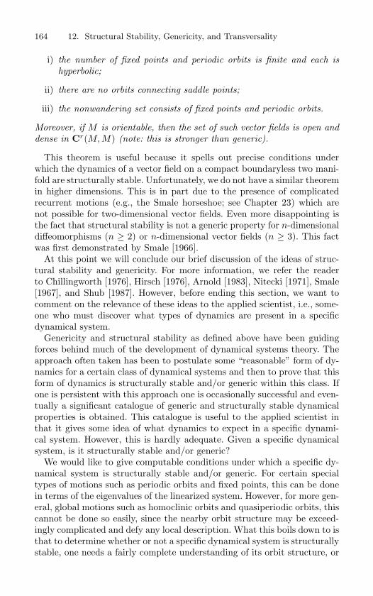
164 12. Structural Stability, Genericity, and Transversality
i) the number of fixed points and periodic orbits is finite and each is
hyperbolic;
ii) there are no orbits connecting saddle points;
iii) the nonwandering set consists of fixed points and periodic orbits.
Moreover, if M is orientable, then the set of such vector fields is open and
dense in Cr(M, M) (note: this is stronger than generic).
This theorem is useful because it spells out precise conditions underwhich the dynamics of a vector field on a compact boundaryless two mani-fold are structurally stable. Unfortunately, we do not have a similar theoremin higher dimensions. This is in part due to the presence of complicatedrecurrent motions (e.g., the Smale horseshoe; see Chapter 23) which arenot possible for two-dimensional vector fields. Even more disappointing isthe fact that structural stability is not a generic property for n-dimensionaldiffeomorphisms (n ≥ 2) or n-dimensional vector fields (n ≥ 3). This factwas first demonstrated by Smale [1966].
At this point we will conclude our brief discussion of the ideas of struc-tural stability and genericity. For more information, we refer the readerto Chillingworth [1976], Hirsch [1976], Arnold [1983], Nitecki [1971], Smale[1967], and Shub [1987]. However, before ending this section, we want tocomment on the relevance of these ideas to the applied scientist, i.e., some-one who must discover what types of dynamics are present in a specificdynamical system.
Genericity and structural stability as defined above have been guidingforces behind much of the development of dynamical systems theory. Theapproach often taken has been to postulate some “reasonable” form of dy-namics for a certain class of dynamical systems and then to prove that thisform of dynamics is structurally stable and/or generic within this class. Ifone is persistent with this approach one is occasionally successful and even-tually a significant catalogue of generic and structurally stable dynamicalproperties is obtained. This catalogue is useful to the applied scientist inthat it gives some idea of what dynamics to expect in a specific dynami-cal system. However, this is hardly adequate. Given a specific dynamicalsystem, is it structurally stable and/or generic?
We would like to give computable conditions under which a specific dy-namical system is structurally stable and/or generic. For certain specialtypes of motions such as periodic orbits and fixed points, this can be donein terms of the eigenvalues of the linearized system. However, for more gen-eral, global motions such as homoclinic orbits and quasiperiodic orbits, thiscannot be done so easily, since the nearby orbit structure may be exceed-ingly complicated and defy any local description. What this boils down to isthat to determine whether or not a specific dynamical system is structurallystable, one needs a fairly complete understanding of its orbit structure, or
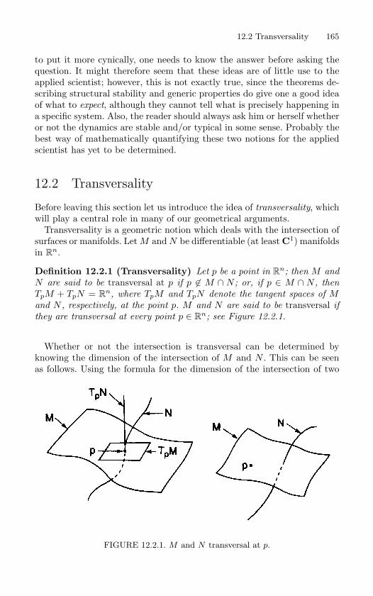
12.2 Transversality 165
to put it more cynically, one needs to know the answer before asking thequestion. It might therefore seem that these ideas are of little use to theapplied scientist; however, this is not exactly true, since the theorems de-scribing structural stability and generic properties do give one a good ideaof what to expect, although they cannot tell what is precisely happening ina specific system. Also, the reader should always ask him or herself whetheror not the dynamics are stable and/or typical in some sense. Probably thebest way of mathematically quantifying these two notions for the appliedscientist has yet to be determined.
12.2 Transversality
Before leaving this section let us introduce the idea of transversality, whichwill play a central role in many of our geometrical arguments.
Transversality is a geometric notion which deals with the intersection ofsurfaces or manifolds. Let M and N be differentiable (at least C1) manifoldsin R
n.
Definition 12.2.1 (Transversality) Let p be a point in Rn; then M and
N are said to be transversal at p if p ∈ M ∩ N ; or, if p ∈ M ∩ N , then
TpM + TpN = Rn, where TpM and TpN denote the tangent spaces of M
and N , respectively, at the point p. M and N are said to be transversal if
they are transversal at every point p ∈ Rn; see Figure 12.2.1.
Whether or not the intersection is transversal can be determined byknowing the dimension of the intersection of M and N . This can be seenas follows. Using the formula for the dimension of the intersection of two
FIGURE 12.2.1. M and N transversal at p.
166 12. Structural Stability, Genericity, and Transversality
vector subspaces we have
dim(TpM + TpN) = dimTpM + dimTpN − dim(TpM ∩ TpN). (12.2.1)
From Definition 12.2.1, if M and N intersect transversely at p, then wehave
n = dimTpM + dimTpN − dim(TpM ∩ TpN). (12.2.2)
Since the dimensions of M and N are known, then knowing the dimensionof their intersection allows us to determine whether or not the intersectionis transversal.
Note that transversality of two manifolds at a point requires more thanjust the two manifolds geometrically piercing each other at the point. Con-sider the following example.
Example 12.2.1. Let M be the x axis in R2, and let N be the graph of the
function f(x) = x3; see Figure 12.2.2. Then M and N intersect at the origin in
R2, but they are not transversal at the origin, since the tangent space of M is
just the x axis and the tangent space of N is the span of the vector (1, 0); thus,
T(0,0)N = T(0,0)M and, therefore, T(0,0)N + T(0,0)M = R2.
End of Example 12.2.1
FIGURE 12.2.2. Nontransversal manifolds.
The most important characteristic of transversality is that it persistsunder sufficiently small perturbations. This fact will play a useful role inmany of our geometric arguments; we remark that a term often used syn-onymously for transversal is general position, i.e., two or more manifoldswhich are transversal are said to be in general position.
Let us end this section by giving a few “dynamical” examples of transver-sality.
Example 12.2.2. Consider a hyperbolic fixed point of a Cr, r ≥ 1, vector
field on Rn. Suppose the matrix associated with the linearization of the vector
12.3 Exercises 167
field about the fixed point has n − k eigenvalues with positive real part and
k eigenvalues with negative real part. Thus this fixed point has an (n − k)-
dimensional unstable manifold and a k-dimensional stable manifold. If these two
manifolds intersect in a point, other than the fixed point, then by uniqueness of
solutions and invariance of the manifolds, they must intersect along a (at least)
one-dimensional orbit. Hence, by (12.2.2), the intersection cannot be transverse.
End of Example 12.2.2
Example 12.2.3. Suppose the vector field of Example 12.2.2 is Hamiltonian
so that all orbits are restricted to lie in (n − 1)-dimensional “energy” surfaces
given by the level sets of the Hamiltonian. Then it is possible for the stable and
unstable manifolds of the hyperbolic fixed point to intersect transversely in the(n − 1)-dimensional energy surface.
End of Example 12.2.3
Example 12.2.4. Consider a hyperbolic periodic orbit of a Cr, r ≥ 1, vector
field on Rn. Suppose that the Poincare map associated with the periodic orbit
linearized about the fixed point has n − k − 1 eigenvalues with modulus greater
than one and k eigenvalues with modulus less than one. Then the periodic orbit
has an (n − k)-dimensional unstable manifold and a (k + 1)-dimensional stable
manifold. Therefore, by (12.2.2), if these manifolds intersect transversely, the
dimension of the intersection must be one. This is possible without violating
uniqueness of solutions and invariance of the manifolds.
End of Example 12.2.4
12.3 Exercises1. Consider the space of linear, autonomous vector fields on R
2.
(a) Give a rigorous definition of this space. Define a norm on this space.
(b) Describe the set of structurally stable vector fields on this space. Is this set aresidual set?
2. Consider the unit interval in R. Show that the irrational numbers are a residual subset.Show that the rational numbers are not a residual subset.
3. Consider the unit interval in R. Construct an open and dense subset having Lebesguemeasure smaller than any specified number. Construct a residual subset with Lebesguemeasure zero. (Hint: for help, see Hunt et al. [1992].)
4. Discuss the idea of structural stability of the following vector fields and maps.
a) θ1 = ω1,
θ2 = ω2,(θ1, θ2) ∈ S
1 × S1.
b) x = 1,y = 2,
(x, y) ∈ R2.
c)x = y,y = x − x3,
(x, y) ∈ R2.
168 12. Structural Stability, Genericity, and Transversality
d)x = y,y = x − x3 − y,
(x, y) ∈ R2.
e) θ → θ + ω, θ ∈ S1.
f) θ → θ + ω + ε sin θ, ε small, θ ∈ S1.
5. Consider an autonomous vector field on R2 having a hyperbolic sink equilibrium point
and a hyperbolic saddle equilibrium point.
(a) Can the unstable manifold of the saddle intersect the stable manifold of the sinktransversely?
(b) Can the stable manifold of the saddle intersect the stable manifold of the sinktransversely?
6. Consider an autonomous vector field on R3 having a hyperbolic periodic orbit and a
hyperbolic saddle equilibrium point having a one dimensional stable manifold and atwo dimensional unstable manifold.
(a) Can the unstable manifold of the saddle intersect the stable manifold of theperiodic orbit transversely?
(b) Can the stable manifold of the saddle intersect the unstable manifold of theperiodic orbit transversely?
13
Lagrange’s Equations
Up to this point in the book we have been studying general dynamicalsystems, e.g., , x = f(x), where f(x) is just Cr. In this, and the followingfour chapters, we will study dynamical systems with special structure; La-grangian systems, Hamiltonian systems, gradient vector fields, reversiblesystems, and asymptotically autonomous vector fields. We will see that theparticular special structure greatly constrains the types of dynamics thatare allowed, and it also provides techniques of analysis that are particularto the special structure. These particular types of structure are importantbecause they do arise in a variety of applications.
In this chapter we will derive and discuss the properties of Lagrange’seuations of motion or Lagrangian dynamical systems for a system of P parti-cles each having constant mass mp and located at position rp = (xp, yp, zp),p = 1, . . . , P , where (xp, yp, zp) denote the standard cartesian coordinates.
The issue of the correct choice of coordinates is central to the under-standing of many problems in dynamical systems theory. Indeed, manytechniques, such as normal form theory and invariant manifold theory, areprimarily concerned with finding a coordinate system in which the dynam-ical system assumes the ”simplest” form, or the dimensionality (i.e., in thiscontext, we mean the number of equations) of the system is reduced.
For a system of P point masses moving under the influence of externaland internal forces it may be that there are certain functional relationsamong some of the coordinate components. In this case we say that themotion of the point masses is subject to certain constraints. For example,a particle could be constrained to move on the surface of a sphere, on aninclined plane, etc.
Suppose the system of P particles is such that C functional relationsmust be satisfied by the coordinates of the particles. We represent theseconstraints as follows:
φi (x1, y1, z1, . . . , xP , yP , zP , t) , i = 1, . . . , C. (13.0.1)
Constraints that are represented as functions of the coordinates and timein this manner are referred to as holonomic constraints. In this case we saythat the system has N = 3P−C degrees of freedom. That is, the position ofall the particles in the system can be specified by choosing N independent
coordinates. In other words, the number of degrees of freedom of a systemis the number of independent coordinates needed to specify the positions
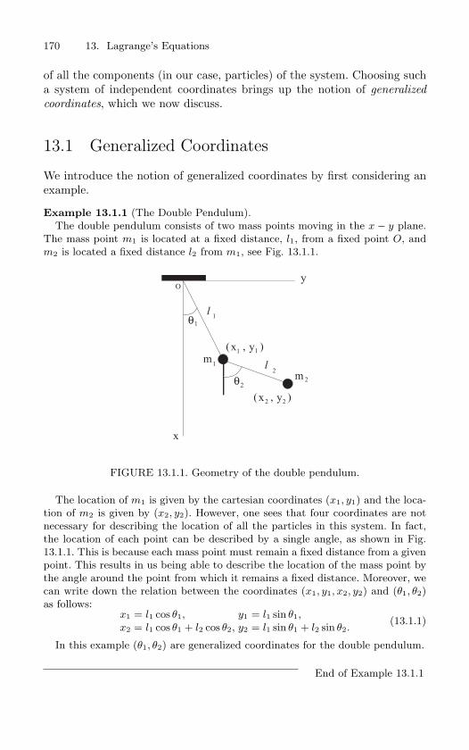
170 13. Lagrange’s Equations
of all the components (in our case, particles) of the system. Choosing sucha system of independent coordinates brings up the notion of generalized
coordinates, which we now discuss.
13.1 Generalized Coordinates
We introduce the notion of generalized coordinates by first considering anexample.
Example 13.1.1 (The Double Pendulum).
The double pendulum consists of two mass points moving in the x − y plane.
The mass point m1 is located at a fixed distance, l1, from a fixed point O, and
m2 is located a fixed distance l2 from m1, see Fig. 13.1.1.
O
x
y
x y( ),1 1
x y( ),2 2
l 1θ1
2θ2
l2m
1m
FIGURE 13.1.1. Geometry of the double pendulum.
The location of m1 is given by the cartesian coordinates (x1, y1) and the loca-
tion of m2 is given by (x2, y2). However, one sees that four coordinates are not
necessary for describing the location of all the particles in this system. In fact,
the location of each point can be described by a single angle, as shown in Fig.
13.1.1. This is because each mass point must remain a fixed distance from a given
point. This results in us being able to describe the location of the mass point by
the angle around the point from which it remains a fixed distance. Moreover, we
can write down the relation between the coordinates (x1, y1, x2, y2) and (θ1, θ2)
as follows:x1 = l1 cos θ1, y1 = l1 sin θ1,x2 = l1 cos θ1 + l2 cos θ2, y2 = l1 sin θ1 + l2 sin θ2.
(13.1.1)
In this example (θ1, θ2) are generalized coordinates for the double pendulum.
End of Example 13.1.1
13.1 Generalized Coordinates 171
A set of coordinates that contain the minimum number of independentcoordinates needed to specify all the positions of a set of particles is re-ferred to as generalized coordinates, and denoted by (q1, . . . , qN ). General-ized coordinates may be distances, angles, or quantities relating them. Theinteger N is referred to as the number of degrees-of-freedom of a system.So a system is said to have N degrees-of-freedom if the positions of allits components can be described by N independent (generalized) coordi-nates. The space of generalized coordinates of a system is often referred toas the configuration space of the system (the reader should contrast thiswith the notion of “phase space”). Furthermore, we refer to (q1, . . . , qN ) asgeneralized velocities.
Getting back to the notion of constraints, one could also say that theconstraints imposed on a system are holonomic if it is possible to choose aset of independent generalized coordinates to describe the position of theset of particles. The issue of constraints is very important in dynamics,and is beyond the scope of this book. Excellent discussions of constraints,both holonomic and non-holonomic, can be found in Sommerfeld [1952],Whittaker [1904], and Arnold [1978]. One of the strengths of the Lagrangianform of dynamics is that it deals with constraints in a very simple manner,especially holonomic constraints. In this chapter we will deal exclusivelywith holonomic constraints.
The relationship between the original cartesian position coordinates ofeach particle and the generalized coordinates (see, as an example, eq.(13.1.1)) is expressed in the following form:
xp = xp(q1, . . . , qN , t),yp = yp(q1, . . . , qN , t),zp = zp(q1, . . . , qN , t), p = 1, . . . , P, (13.1.2)
or, in vector notation
rp = rp(q1, . . . , qN , t), p = 1, . . . , P. (13.1.3)
In the derivation of Lagrange’s equations of motion two relationshipsbetween the derivatives of the coordinates and velocities and the corre-sponding generalized coordinates and velocities will be particularly useful,so we want to derive them now.
Differentiating (13.1.3) with respect to time gives:
rp =∂rp
∂q1q1 + · · ·+ ∂rp
∂qNqN +
∂rp
∂t=
N∑i=1
(∂rp
∂qiqi +
∂rp
∂t
), (13.1.4)
from which it follows that∂rp
∂qi=
∂rp
∂qi. (13.1.5)
172 13. Lagrange’s Equations
If we assume that the second order partial derivative of (13.1.3) existand are continuous then the order of differentiation with respect to anytwo variables can be interchanged. In this case we have
d
dt
(∂rp
∂qi
)=
∂rp
∂qi, (13.1.6)
which can be derived directly from (13.1.4) with a bit of work, which weleave for the reader.
13.2 Derivation of Lagrange’s Equations
Now we are ready to derive Lagrange’s equations of motion. Newton’s sec-ond law of motion for the point mass mp acted on by the force Fp is givenby
mprp = Fp. (13.2.1)
Here the force Fp acting on the particle p could be due to internal forces ofinteraction amongst the particles (such as electrical or gravitational interac-tions) or external forces. This distinction is not important in the derivationof Lagrange’s equations.
Imagine each point p is subject to a displacement drp. Then the workdone on the system of particles is given by
P∑p=1
mprp · drp =P∑
p=1
Fp · drp. (13.2.2)
This is the key expression in our derivation of Lagrange’s equations (al-though there are other ways in which Lagrange’s equations may be derived,see Sommerfeld [1952]). Computing the differential of (13.1.3) gives:
drp =N∑
i=1
(∂rp
∂qidqi +
∂rp
∂tdt
). (13.2.3)
Substituting (13.2.3) into the left hand side of (13.2.2) gives:
P∑p=1
mprp · drp =P∑
p=1
N∑i=1
mprp ·(
∂rp
∂qidqi +
∂rp
∂tdt
)
=P∑
p=1
N∑i=1
mp
(d
dt
(rp ·
∂rp
∂qi
)− rp ·
d
dt
∂rp
∂qi
)dqi
+mprp ·∂rp
∂tdt using (13.1.5) and (13.1.6)
13.2 Derivation of Lagrange’s Equations 173
=P∑
p=1
N∑i=1
(d
dt
∂
∂qi
(12mprp · rp
)− ∂
∂qi
(12mprp · rp
))dqi
+mprp ·∂rp
∂tdt,
=N∑
i=1
(d
dt
(∂T
∂qi
)− ∂T
∂qi
)dqi +
P∑p=1
mprp ·∂rp
∂tdt, (13.2.4)
where
T =12
P∑p=1
mprp · rp, (13.2.5)
is the kinetic energy of the system of P particles.Substituting (13.2.3) into the right hand side of (13.2.2) gives:
P∑p=1
Fp · drp =N∑
i=1
P∑p=1
Fp ·∂rp
∂qidqi +
P∑p=1
Fp ·∂rp
∂tdt,
=N∑
i=1
Φidqi +P∑
p=1
Fp ·∂rp
∂tdt, (13.2.6)
where
Φi ≡P∑
p=1
Fp ·∂rp
∂qi, (13.2.7)
is referred to as the generalized force associated with the generalized coor-dinate qi.
Since (13.2.6) and (13.2.4) are equal (from (13.2.2)), subtracting thesetwo equations gives:
N∑i=1
((d
dt
(∂T
∂qi
)− ∂T
∂qi
)− Φi
)dqi = 0. (13.2.8)
Since we are considering only holonomic constraints the dqi are all inde-pendent displacements. Then we must have:
d
dt
(∂T
∂qi
)− ∂T
∂qi= Φi, i = 1, . . . , N. (13.2.9)
These are Lagrange’s equations of motion.If the forces are derivable from a potential function, i.e.,
Φi = −∂V
∂qi, (13.2.10)
174 13. Lagrange’s Equations
then we can write Lagrange’s equations in a more compact form. We definethe Lagrangian function (or, just the “Lagrangian”) as
L = T − V. (13.2.11)
Then, since V is only a function of the qi, we have
∂L
∂qi=
∂T
∂qi,
and Lagrange’s equations become:
d
dt
(∂L
∂qi
)− ∂L
∂qi= 0, i = 1, . . . , N. (13.2.12)
From (13.1.3), (13.1.4), (13.2.5), and (13.2.7) we see that the Lagrangianhas the following functional dependencies with respect to the generalizedcoordinates:
L = L(q1, . . . , qN , q1, . . . , qN , t). (13.2.13)
In some cases it may be convenient to adopt a shorthand notation for(13.2.12). Let
q ≡ (q1, . . . , qN ), q ≡ (q1, . . . , qN ).
Then we write (13.2.12) as
d
dt
(∂L
∂q
)− ∂L
∂q= 0, (13.2.14)
where (13.2.12) is the definition of (13.2.14).We now give an example where we derive the equations of motion of a
system using Lagrange’s equations.
Example 13.2.1 (The Pendulum).
As an example, we compute the Lagrangian, and Lagrange’s equations of mo-
tion, for the pendulum, as illustrated in Fig. 13.2.1. We assume that all forces
acting on the pendulum are conservative (e.g., there is no drag force as the pen-
dulum moves through air).
We choose as the generalized coordinate (the reader should convince him or
herself that this is a one degree-of-freedom system) the angle θ between the
vertical line OA and the string, OB, of the pendulum. If l denotes the length of
OB then the kinetic energy is given by
T =1
2mv2
=1
2m(lθ)2 =
1
2ml2θ2.
Next we compute the potential energy, V , We take as a reference line the
horizontal line through the lowest point of the pendulum, denoted A. Then the
potential energy due to gravity is given by
V = mg (OA − OC) = mg (l − l cos θ) = mgl(1 − cos θ).
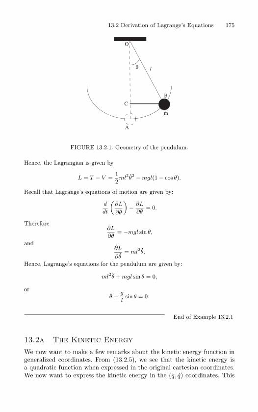
13.2 Derivation of Lagrange’s Equations 175
O
C
A
B
m
θ l
FIGURE 13.2.1. Geometry of the pendulum.
Hence, the Lagrangian is given by
L = T − V =1
2ml2θ2 − mgl(1 − cos θ).
Recall that Lagrange’s equations of motion are given by:
d
dt
(∂L
∂θ
)− ∂L
∂θ= 0.
Therefore∂L
∂θ= −mgl sin θ,
and∂L
∂θ= ml2θ.
Hence, Lagrange’s equations for the pendulum are given by:
ml2θ + mgl sin θ = 0,
or
θ +g
lsin θ = 0.
End of Example 13.2.1
13.2a The Kinetic EnergyWe now want to make a few remarks about the kinetic energy function ingeneralized coordinates. From (13.2.5), we see that the kinetic energy isa quadratic function when expressed in the original cartesian coordinates.We now want to express the kinetic energy in the (q, q) coordinates. This
176 13. Lagrange’s Equations
is done by substituting (13.1.4) into (13.2.5), and then after some routinealgebra we obtain:
T =N∑
i=1
N∑j=1
mi,j(q, t)qiqj +N∑
i=1
ni(q, t)qi + f(q, t), (13.2.15)
where
mi,j(q, t) =P∑
p=1
∂rp
∂qi· ∂rp
∂qj,
ni(q, t) = 2P∑
p=1
∂rp
∂qi· ∂rp
∂t,
f(q, t) =P∑
p=1
∂rp
∂t· ∂rp
∂t.
Note that if the transformation between the original coordinates and thegeneralized coordinates (i.e., (13.1.3)) is independent of time, then the lasttwo sums in (13.2.15) do not occur.
13.3 The Energy Integral
In the case where the generalized forces are derivable from a potentialfunction (so that Lagrange’s equations are given by (13.2.12)), and the La-grangian is independent of time, Lagrange’s equations possess and integralof the motion, called the energy integral, which is given by:
E =N∑
i=1
∂L
∂qiqi − L. (13.3.1)
We prove this quantity is an integral for Lagrange’s equations through thefollowing calculation:
dE
dt=
N∑i=1
((d
dt
(∂L
∂qi
))qi +
∂L
∂qi
d
dtqi
)− dL
dt,
=N∑
i=1
((d
dt
(∂L
∂qi
))qi +
∂L
∂qiqi −
∂L
∂qiqi −
∂L
∂qiqi
)− ∂L
∂t,
=N∑
i=1
((d
dt
∂L
∂qi
)− ∂L
∂qi
)qi −
∂L
∂t,
= −∂L
∂t, using (13.2.12), (13.3.2)
13.4 Momentum Integrals 177
So if L does not depend on time then we have
dE
dt= 0.
13.4 Momentum Integrals
In the previous section we saw that when the Lagrangian is time indepen-dent there is an integral for the system, the energy integral. Similarly, wewill now see that when the Lagrangian does not depend upon a certaincoordinate, say qk (although it may depend on qk), then there is also anintegral for the system, called a momentum integral. The coordinate qk isreferred to as a cyclic or ignorable coordinate.
In particular, suppose
L = L(q1, . . . , qk−1, qk+1, . . . , qN , q1, . . . , qN , t).
Then clearly∂L
∂qk= 0,
and therefore it follows from Lagrange’s equations that
d
dt
(∂L
∂qk
)= 0.
Hence∂L
∂qk= βk = constant.
In general the quantity ∂L∂qk
is referred to as the kth component of mo-
mentum (or generalized momentum), and is denoted by pk. It plays animportant role in Hamilton’s equations, which we now discuss.
13.5 Hamilton’s Equations
Now we will show how Hamilton’s equations can be derived using the La-grangian.
The function
H(q, p, t) =N∑
i=1
piqi − L(q, q, t), (13.5.1)
is defined to be the Hamiltonian function (or just “Hamiltonian”) of thesystem. Note that it is just the energy integral given in (13.3.1) where
pi ≡∂L
∂qi, and p = (p1, . . . , pN ). (13.5.2)
178 13. Lagrange’s Equations
This is an important point because the left hand side of (13.5.1) is denotedas a function of q, p, and t, rather than q, q, and t. This is accomplishedby using (13.5.2) to solve for q as a function of p, and then substituting theresult for q into (13.5.1), resulting in a function depending on q, p, and t.Note that differentiating (13.5.2) with respect to time and using (13.1.5)gives
pi =∂L
∂qi. (13.5.3)
Computing the differential of (13.5.1) gives:
dH(q, p, t) =N∑
i=1
d (piqi)− dL,
=N∑
i=1
qidpi + pidqi −∂L
∂qidqi −
∂L
∂qidqi −
∂L
∂tdt,
=N∑
i=1
qidpi − pidqi −∂L
∂tdt, using (13.5.2) and (13.5.3).
(13.5.4)
Since, as described above, the Hamiltonian is a function of q, p, and t, wehave, in general:
dH(q, p, t) =N∑
i=1
∂H
∂qidqi +
∂H
∂pidpi +
∂H
∂tdt. (13.5.5)
The expressions given in (13.5.4) and (13.5.5) must be equal. Since the qi
and pi are independent (holonomic constraints), equating the coefficientsof dqi and dpi immediately leads to Hamilton’s equations
qi =∂H
∂pi,
pi = −∂H
∂qi, i = 1, . . . , N, (13.5.6)
with the relation∂H
∂t= −∂L
∂t. (13.5.7)
13.6 Cyclic Coordinates, Routh’s Equations, andReduction of the Number of Equations
Now we will describe an elegant procedure due to Routh for reducing thenumber of equations that need to be integrated in the case where we havecyclic coordinates in the Lagrangian.
13.6 Cyclic Coordinates and Routh’s Equations 179
Suppose we have r cyclic coordinates. Without loss of generality (throughrelabeling the coordinates, if necessary) we can suppose these are the firstr coordinates:
q1, . . . , qr︸ ︷︷ ︸cyclic
, qr+1, . . . , qN
. (13.6.1)
Then the Lagrangian has the form
L = L(qr+1, . . . , qN , q1, . . . , qN ), (13.6.2)
and, as we described earlier,
∂L
∂qi= βi = constant, i = 1, . . . , r. (13.6.3)
Using (13.6.3) we can solve for qi, i = 1, . . . , r, as a function ofqr+1, . . . , qN , qr+1, . . . , qN , β1, . . . , βr, t, i.e., we have
qi = qi(qr+1, . . . , qN , qr+1, . . . , qN , β1, . . . , βr, t) i = 1, . . . , r. (13.6.4)
We then form Routh’s function, or the Routhian, defined as follows:
R = L−r∑
i=1
piqi, (13.6.5)
Computing the differential of (13.6.5) gives:
dR =N∑
i=r+1
∂L
∂qidqi +
N∑i=1
∂L
∂qidqi +
∂L
∂tdt−
r∑i=1
(pidqi + qidpi) ,
=N∑
i=r+1
∂L
∂qidqi +
N∑i=r+1
∂L
∂qidqi +
∂L
∂tdt−
r∑i=1
qidpi. (13.6.6)
However, as we described above, in general the Routhian is a function ofqr+1, . . . , qN , qr+1, . . . , qN , β1, . . . , βr, t, where βi = pi, i = 1, . . . , r. Com-puting the differential of the Routhian with these functional dependenciesgives:
dR =N∑
i=r+1
(∂R
∂qidqi +
∂R
∂qidqi
)+
r∑i=1
∂R
∂pidpi +
∂R
∂tdt, (13.6.7)
Now (13.6.6) and (13.6.7) must be equal. Since the coordinates qi, qi andpi are independent we can then equate the coefficients on dqi, dqi and dpi
to obtain Routh’s equations:
∂L
∂qi=
∂R
∂qi,
∂L
∂qi=
∂R
∂qi, i = r + 1, . . . , N, (13.6.8)
180 13. Lagrange’s Equations
with the relationqi = −∂R
∂pi, i = 1, . . . , r. (13.6.9)
Substituting (13.6.8) into Lagrange’s equations (13.2.14) gives:
d
dt
(∂R
∂qi
)− ∂R
∂qi= 0, i = r + 1, . . . , N. (13.6.10)
Hence we solve the N − r equations for qr+1, . . . , qN , qr+1, . . . , qN . We thensubstitute the result into (13.6.9) to obtain qi, i = 1, . . . , r. In turn, thesecan then be integrated (since, now in principle they are known functions oftime once (13.6.10) are solved) to give qi, i = 1, . . . , r. So we see that in thecase where there are r cyclic coordinates the solution of Lagrange’s equa-tions can be “reduced” to the solution of N − r (second order) differentialequations.
13.7 Variational Methods
Trajectories of Lagrange’s and Hamilton’s equations can also be character-ized as extrema of a certain functional defined on paths in configurationand phase space, respectively. This leads to the variational principles of me-chanics, which we now describe. Excellent references with historical surveyscan be found in Sommerfeld [1952] and Arnold [1978]1.
13.7a The Principle of Least ActionLet C denote the set of curves in the configuration space with fixed endpoints, i.e., a “point” in C is a map
t → (q1(t), . . . , qN (t)) ≡ q(t), t0 ≤ t ≤ t1,
and the fixed endpoint condition means that every q(t) ∈ C satisfies q(t0) =q0 and q(t1) = q1. We equip C with the following norm. For q ∈ C, the normof q is defined as
‖ q ‖≡ supt∈[t0,t1], 1≤i≤N
(|qi(t)|+ |qi(t)|) . (13.7.1)
We will need the curves in C to have at least one continuous derivative.
1In most dynamics textbooks the action functional is stated and then it isshown that the extrema correspond to solutions of Lagrange’s equations. Som-merfeld [1952] provides an insightful derivation of the action functional by be-ginning from the principle of virtual work (a differential variational principle, asopposed to the integral variational principles discussed here). See also Arnold[1978] for a similar argument in more modern mathematical language.
13.7 Variational Methods 181
If L(q, q, t) denotes the Lagrangian of a system then the expression de-fined by
Φ(q) =∫ t1
t0
L(q, q, t)dt =∫ t1
t0
L(q1, . . . , qN , q1, . . . , qN , t)dt, (13.7.2)
is called the action. The action is an example of a functional, i.e., a mapfrom C to R. Now we want to define the notion of differentiability of thisfunctional.
Definition 13.7.1 The functional Φ(q) is said to be differentiable at q if
Φ(q +h)−Φ(q) = F +R, where F = F (q, h) is a linear function of h (with
h(t0) = h(t1) = 0 in order to satisfy the fixed end point constraint, and
regarding q as fixed), and R = O(‖ h ‖2). The term linear in h, F (q, h), is
called the differential of Φ.
We now define the notion of an extremal for the action.
Definition 13.7.2 An extremal of the action Φ is a curve q such that
F (q, h) = 0 for all h.
Now we compute the differential of the action functional:
=∫ t1
t0
(L(q + h, q + h, t)dt− L(q, q, t)
)dt,
=∫ t1
t0
N∑i=1
(∂L
∂qihi +
∂L
∂qihi
)dt +O(‖ h ‖2),
=∫ t1
t0
N∑i=1
(∂L
∂qi− d
dt
∂L
∂q
)hidt +
N∑i=1
∂L
∂qihi
∣∣∣∣t1t0
+O(‖ h ‖2),
after integration by parts. (13.7.3)
Now since h(t0) = h(t1) = 0 we see that the differential of the action isgiven by ∫ t1
t0
N∑i=1
(∂L
∂qi− d
dt
∂L
∂q
)hidt. (13.7.4)
Now we set the differential of the action to zero and we can then appeal toa classical result from the calculus of variations (see, e.g., Arnold [1978])that says that (13.7.4) is zero for all hi if and only if
∂L
∂qi− d
dt
∂L
∂q= 0, i = 1, . . . N.
182 13. Lagrange’s Equations
Now these are just Lagrange’s equations of motion, and we arrive at thefollowing result, which is referred to as Hamilton’s principle of least action2.
Theorem 13.7.3 (Hamilton’s Principle of Least Action) The curve
q(t), t0 ≤ t ≤ t1 is a solution of Lagrange’s equations:
d
dt
(∂L
∂qi
)− ∂L
∂qi= 0, i = 1, . . . , N,
if and only if it is an extremal of the action:
Φ(q) =∫ t1
t0
L(q, q, t)dt.
Despite the name “principle of least action” we remark that an extremalof the action need not be a minimum. The only requirement is that thedifferential of the action must vanish on a trajectory.
In the classical mechanics literature there is another common notationfor the differential of the action. Namely,
δ
∫ t1
t0
L(q, q, t)dt, (13.7.5)
and the phrase “first variation’ or just “variation” of the action is used.
13.7b The Action Principle in Phase SpaceThe action principle can also be formulated in phase space.
Let P denote the set of curves in the phase space where the q coordinateshave fixed end points, i.e., a “point” in P is a map
t → (q1(t), . . . , qN (t), p1(t), . . . , pN (t)) ≡ (q(t), p(t)), t0 ≤ t ≤ t1,
and the fixed endpoint condition means that for every curve (q(t), p(t)),the q(t) component satisfies q(t0) = q0 and q(t1) = q1. We equip P withthe following norm. For (q(t), p(t)) ∈ P, the norm of (q(t), p(t)) is definedas
‖ (q(t), p(t)) ‖≡ supt∈[t0,t1], 1≤i≤N
(|qi(t)|+ |qi(t)|, |pi(t)|+ |pi(t)|) . (13.7.6)
We will need the curves in P to have at least one continuous derivative.
2While the name of Hamilton is associated with this integral variational prin-ciple in configuration space, Leibniz, Maupertuis, Euler, and Lagrange also madesignificant contributions. See Sommerfeld [1952].
13.7 Variational Methods 183
Since L =∑N
i=1 piqi−H we can rewrite (13.7.2) and define the followingfunctional on P:∫ t1
t0
(N∑
i=1
piqi −H(q, p, t)
)dt =
∫ t1
t0
(N∑
i=1
pidqi −H(q, p, t)dt
). (13.7.7)
Next we compute the differential of this functional:
∫ t1
t0
(N∑
i=1
(pi + ki)(qi + hi)− piqi −H(q + h, p + k, t) + H(q, p, t)
)dt,
=∫ t1
t0
N∑i=1
(qiki + pihi −
∂H
∂qihi −
∂H
∂piki
)dt +O(‖ (h, k) ‖2),
=∫ t1
t0
(N∑
i=1
(qi −
∂H
∂pi
)ki −
(pi +
∂H
∂qi
)hi
)dt +
N∑i=1
pihi
∣∣∣∣t1t0
+O(‖ (h, k) ‖2), (13.7.8)
where the passage from the second to the third line in (13.7.8) is effectedby integration by parts. Since h(t0) = h(t1) = 0 we see that the differentialof this functional is given by
∫ t1
t0
(N∑
i=1
(qi −
∂H
∂pi
)ki −
(pi +
∂H
∂qi
)hi
)dt. (13.7.9)
Clearly, trajectories of Hamilton’s equations are extrema of (13.7.7). How-ever, the argument that extrema of (13.7.7) are trajectories of Hamilton’sequations requires a bit more care since pi and qi are related in time throughthe equation pi = ∂L
∂qi. Sommerfeld [1952] and Arnold [1978] both address
this issue. Sommerfeld resolves the issue by noting that upon differentiat-ing (13.5.1) with respect to pi one obtains ∂H
∂pi= qi. Hence the first term
in braces in (13.7.9) vanishes. Since the hi are independent for each i,the second term in braces in (13.7.9) must also vanish (applying the sameargument as was used to deduce Hamilton’s principle of least action inconfiguration space). Hence, we have the following result. 3
Theorem 13.7.4 (Hamilton’s Principle of Least Action in PhaseSpace) The curve (q(t), p(t)), t0 ≤ t ≤ t1 is a solution of Hamilton’s
equations:
qi =∂H
∂pi(q, p, t), pi = −∂H
∂qi(q, p, t), i = 1, . . . , N,
3Poincare and Hilbert also studied this functional.
184 13. Lagrange’s Equations
if and only if it is an extremal of the functional:
∫ t1
t0
(N∑
i=1
piqi −H(q, p, t)
)dt.
Rather than the phrase “Hamilton’s principle of least action”, often theshorter phrase “Hamilton’s principle” is used instead. This applies in boththe configuration space and phase space formulations.
13.7c Transformations that Preserve the Form ofHamilton’s Equations
We now consider an application of the action principle in phase space.Consider the Hamiltonian
H(q, p, t), (13.7.10)
and the associated Hamilton’s equations:
q =∂H
∂p(q, p, t),
p = −∂H
∂q(q, p, t). (13.7.11)
Suppose we have a transformation of coordinates of the form
Q = Q(q, p, t),P = P (q, p, t), (13.7.12)
which we assume can be inverted (viewing t as fixed) to yield
q = q(Q,P, t),p = p(Q,P, t). (13.7.13)
Clearly, (13.7.13) can be substituted into (13.7.10) so that the Hamilto-nian in the original (q, p) coordinates can be written as a function of the(Q,P ) coordinates:
H(q, p, t) = H(Q,P, t). (13.7.14)
However, it is not at all clear that this transformation preserves the formof Hamilton’s equations in the sense that
Q =∂H
∂P(Q,P, t),
P = −∂H
∂Q(Q,P, t). (13.7.15)
13.7 Variational Methods 185
Now we want to derive conditions on the transformation (13.7.12) so that(13.7.15) holds, and we will do this using Hamilton’s principle of leastaction in phase space.
If (13.7.15) holds in the (Q,P ) coordinates then we must have
δ
∫ t1
t0
N∑i=1
PidQi − Hdt = 0,
and therefore
δ
∫ t1
t0
N∑i=1
pidqi −Hdt = δ
∫ t1
t0
N∑i=1
PidQi − Hdt = 0, (13.7.16)
or
δ
∫ t1
t0
N∑i=1
pidqi − PidQi − (H − H)dt = 0,
from which it follows that
dF (q,Q, t) =N∑
i=1
pidqi −N∑
i=1
PidQi + (H − H)dt, (13.7.17)
for some function F (q,Q, t). This function is referred to as the generat-
ing function of the transformation (13.7.12). Writing out the terms of thedifferential of the left hand side of (13.7.17) gives
N∑i=1
∂F
∂qidqi +
N∑i=1
∂F
∂QidQi +
∂F
∂tdt =
N∑i=1
pidqi −N∑
i=1
PidQi + (H − H)dt,
from which it follows that
pi =∂F
∂qi,
Pi = − ∂F
∂Qi,
H = H +∂F
∂t, (13.7.18)
So when F is known (13.7.18) gives the relation between the “old” coordi-nates (q, p), the “new” coordinates (P, Q), and the Hamiltonian. Note thatif the system does not depend explicitly on time then the “new” Hamilto-nian function is the same as the “old” Hamiltonian function. Transforma-tions of coordinates given by (13.7.18) which preserve the form of Hamil-ton’s equations as described above are referred to as canonical transforma-
tions or symplectic transformations (cf. Section 14.4). 4
4The reader should be aware of how the terms and phrases “function”, “map”,“coordinate transformation”, and “operator” are often used interchangeably.
186 13. Lagrange’s Equations
In some situations it may be more convenient to express the generatingfunction not in terms of the old and new coordinates (i.e., in terms of qand Q), but rather in terms of the old coordinates q and the new momentaP . This can be accomplished by rewriting (13.7.17) as
d
(F +
N∑i=1
PiQi
)=
N∑i=1
pidqi +N∑
i=1
QidPi + (H − H)dt, (13.7.19)
We express the argument of the differential on the left hand side of (13.7.19)as a function of q, P , t, which can be viewed as a new generating functionG(q, P, t). Applying the same argument as above gives the relations
pi =∂G
∂qi,
Qi =∂G
∂Pi,
H = H +∂G
∂t. (13.7.20)
The reader should compare the discussion in this section with that inSection 14.4.
13.7d Applications of Variational MethodsIn recent years variational methods have been developed into a powerfuland rigorous mathematical tool. Examples of some applications are givenbelow. Kozlov [1985] provides an excellent survey of the application ofvariational methods in mechanics.
Existence of Periodic Orbits. There is a vast literature on the use ofvariational methods for proving the existence of periodic orbits. SeeRabinowitz [1978] and Struwe [1990] and the references therein.
Existence of Homoclinic Orbits. In recent years variational methodshave been developed for proving the existence of homoclinic orbits.See, e.g., Zelati et al. [1990]
Existence of Invariant Tori. A proof of the KAM theorem (which isconcerned with the existence of invariant tori in perturbations of in-tegrable Hamiltonian systems) by variational methods is given bySalamon and Zehnder [1989].
Existence of Heteroclinic Orbits. The existence of heteroclinic orbitsare believed by many to be a key mechanism for global instabilities inHamiltonian systems (such as “Arnold diffusion”). See, e.g., Mather[1993] and Bessi [1997].
13.8 The Hamilton-Jacobi Equation 187
Existence of Chaos. Sere [1993] has used variational methods to con-struct a chaotic invariant set modeled on the Bernoulli shift.
Numerical Integration of Lagrange’s Equations. Hamilton’s princi-ple can be used to derive a class of numerical methods for solvingLagrange’s equations. An excellent background for this subject, aswell as a literature review, can be found in Lewis and Kostelic [1996]
13.8 The Hamilton-Jacobi Equation
We now consider the action integral (or functional) defined in (13.7.2) froma different point of view. The action as defined in (13.7.2) is a functionaldefined on the set of curves in configuration space having the same end-points. We now want to view this integral as defined on extremals (i.e., ontrajectories of Lagrange’s equations) and as a function of the endpoint ofthe extremal. In order to make this precise we will need to adopt a slightlydifferent notation.
Let q(t) denote an extremal of (13.7.2) with q(t0) = q0 and q(t) = q.Then we define
S(q, t) =∫ t
t0
L(q(τ), ˙q(τ), τ)dτ. (13.8.1)
In this way we view the action as a function of the endpoint of an extremalof (13.7.2) (and we view q0 and t0 as fixed). Arnold [1978] discusses anumber of technical difficulties that can arise in this definition.
Recalling (13.7.3), the differential of (13.8.1) (where variations in q, butnot t are considered) is given by
dS(q, t)h =∫ t
t0
N∑i=1
(∂L
∂qi− d
dt
∂L
∂qi
)hidt +
N∑i=1
∂L
∂qihi
∣∣∣∣tt0
. (13.8.2)
Now since q(t) is an extremal the first term vanishes, and since q(t0) = q0is fixed for each extremal under consideration, (13.8.2) reduces to
dS(q, t)h =N∑
i=1
∂L
∂qihi =
N∑i=1
pihi. (13.8.3)
Since only q (and not t) was varied in computing the differential of S(q, t)we immediately obtain the relation
pi =∂S
∂qi, i = 1, . . . , N. (13.8.4)
From (13.8.1) we havedS
dt= L, (13.8.5)
188 13. Lagrange’s Equations
and therefore
dS
dt= L =
N∑i=1
∂S
∂qiqi +
∂S
∂t,
=N∑
i=1
piqi +∂S
∂t, (13.8.6)
Equation (13.8.6) can be rewritten as
∂S
∂t+ H(q, p, t) = 0, (13.8.7)
or∂S
∂t+ H
(q,
∂S
∂q, t
)= 0, (13.8.8)
Equation (13.8.8) is a partial differential equation for the function S(q, t)which is known as the Hamilton-Jacobi equation. From a solution of theHamilton-Jacobi equation one can obtain the trajectories of the correspond-ing Hamilton’s canonical equations. We now describe this procedure, butfirst we need a definition.
Definition 13.8.1 (Complete Integral of the Hamilton-JacobiEquation) If
φ(q1, . . . , qN , t; a1, . . . , aN ) ≡ φ(q, t; a),
is a solution of (13.8.8), depending on the N constants a = (a1, . . . , aN )such that
det(
∂2φ
∂q∂a
) = 0,
in the domain of interest, then
S ≡ φ + α,
where α is a constant, is said to be a complete integral of (13.8.8).
Now we prove the theorem that also provides a procedure for constructingthe trajectories of Hamilton’s canonical equations from a complete integralof the Hamilton-Jacobi equation.
Theorem 13.8.2 If a complete integral:
S ≡ φ(q1, . . . , qN , t; a1, . . . , aN ) + α,
is known for the Hamilton-Jacobi equation (13.8.8):
∂S
∂t+ H
(q,
∂S
∂q, t
)= 0,
13.8 The Hamilton-Jacobi Equation 189
then from the equations
∂φ
∂ai= bi,
∂φ
∂qi= pi, i = 1, . . . , N, (13.8.9)
with the 2N arbitrary constants ai, bi, one obtains (implicitly) the 2N -
parameter family of solutions of Hamilton’s equations:
qi =∂H
∂pi, pi = −∂H
∂qi, i = 1, . . . , N. (13.8.10)
Proof: The proof is taken from Courant and Hilbert [1962]. Since we areassuming that
det(
∂2φ
∂q∂a
) = 0,
then we can solve the N equations
∂φ
∂ai= bi,
for qi as a function of t and the 2N constants ai, bi. If we substitute thesefunctions into
∂φ
∂qi= pi,
then we obtain pi as functions of t and the 2N constants ai, bi.Now we need to show that the solutions obtained in this way are solutions
of Hamilton’s equations.We begin by differentiating the equation ∂φ
∂ai= bi with respect to t to
obtain:∂2φ
∂t∂ai+
N∑j=1
∂2φ
∂qj∂ai
dqj
dt= 0. (13.8.11)
We next differentiate ∂φ∂t + H(q, ∂φ
∂q , t) = 0 with respect to ai to obtain:
∂2φ
∂t∂ai+
N∑j=1
∂H
∂pj
∂2φ
∂qj∂ai= 0. (13.8.12)
Now we subtract (13.8.11) from (13.8.12), and use the fact thatdet
(∂2φ∂q∂a
) = 0 to obtain
qj =∂H
∂pj, j = 1, . . . , N.
190 13. Lagrange’s Equations
Next we need to show that the functions we obtained satisfy pi = −∂H∂qi
.The argument is similar to the one just given. We first differentiate theequation ∂φ
∂qi= pi with respect to t to obtain:
dpi
dt=
∂2φ
∂t∂qi+
N∑j=1
∂2φ
∂qi∂qj
dqj
dt. (13.8.13)
We next differentiate ∂φ∂t + H(q, ∂φ
∂q , t) = 0 with respect to qi to obtain:
0 =∂2φ
∂t∂qi+
N∑j=1
∂H
∂pj
∂2φ
∂qj∂qi+
∂H
∂qi, (13.8.14)
We have already shown that our functions satisfy qj = ∂H∂pj
, which wesubstitute into (13.8.14). Then we subtract (13.8.14) from (13.8.13) to im-mediately obtain:
pi = −∂H
∂qi, i = 1, . . . , N.
This completes the proof of the theorem.
Example 13.8.1. Now we will give an application of the Hamilton-Jacobi
method by solving for the trajectories of the simple harmonic oscillator.
The Hamiltonian for the simple harmonic oscillator is given by:
H =p2
2+
ω2
2q2. (13.8.15)
Substituting p = ∂S∂q
into (13.8.15), the Hamilton-Jacobi equation is found to be:
∂S
∂t+
1
2
(∂S
∂q
)2
+1
2ω2q2
= 0. (13.8.16)
Now we need to find a complete integral of the Hamilton-Jacobi equation. We
assume a solution of the form:
S(q, t) = S1(q) + S2(t). (13.8.17)
Substituting (13.8.17) into (13.8.16) gives:
−dS2
dt=
1
2
(dS1
dq
)2
+1
2ω2q2.
Now the left hand side of this equation is a function of t and the right hand side
is a function of q. For equality to hold, each side must be equal to a constant, a:
−dS2
dt=
1
2
(dS1
dq
)2
+1
2ω2q2
= a.
13.8 The Hamilton-Jacobi Equation 191
Then1
2
(dS1
dq
)2
+1
2ω2q2
= a,
yields
S1 =
∫ √2
(a − 1
2ω2q2
)dq,
and
−dS2
dt= a,
yields
S2 = −at.
Therefore
S(q, t; a) =
∫ √2
(a − 1
2ω2q2
)dq − at. (13.8.18)
With a solution of the Hamilton-Jacobi equation in hand, we can now follow
the procedure described in Theorem 13.8.2 and obtain the solutions of Hamilton’s
equations.
We set∂S
∂a= b =
1√2
∫dq√
a − 12ω2q2
− t. (13.8.19)
Computing the integral gives:
1
ωsin
−1(
qω√2a
)= t + b,
or,
q(t) =
√2a
ωsin ω(t + b).
The expression for p(t) is obtained through the relation
p =∂S
∂q.
The constants a and b are determined when the initial conditions for the trajec-
tory are chosen5.
End of Example 13.8.1
5In deriving the equation for S1 we took a square root, for which there is achoice of sign. The reader should check that we have not missed something hereand, if not, why not?
192 13. Lagrange’s Equations
13.8a Applications of the Hamilton-JacobiEquation
The main reason for developing the Hamilton-Jacobi equation is that ithas plays a role in a large variety of applications nowadays. Accordingly,it is impossible to make more than a feeble attempt at a survey of theapplications6. Nevertheless, we will provide a few pointers to the literaturethat are relevant to dynamical systems theory.
Courant and Hilbert [1962] provides a mathematically gentle, andstraightforward, introduction to the Hamilton-Jacobi partial differentialequation. The books of Benton [1977] and Rund [1966] provide furtherreferences and the monographs of Lions [1982] and Barles [1994] providea deeper look at the mathematics. Recent papers describing the asymp-totic behavior of solution of the Hamilton-Jacobi equation are Barles andSouganidis [2000a,b], and Roquejoffre [2001]. Recently there has been veryinteresting work involving generalizing the work of Aubry [1983a,b] andMather [1982], [1984], [1986] on twist maps to other settings. See Fathi[1997], Evans and Gomes [2001], and Gomes [2001 a,b,c]. The Hamilton-Jacobi equation has been used to study the existence of homoclinic andheteroclinic orbits in near integrable systems. See Fathi [1998], Gallavottiet al. [2000], Rudnev and Wiggins [1999], [2000], and Sauzin [2001].
13.9 Exercises1. Give a set of generalized coordinates needed to completely specify the motion of each
of the following systems:
(a) a particle constrained to move on an ellipse,
(b) a particle constrained to move on the surface of a sphere,
(c) a pendulum that is not confined to a plane, i.e., it can move in three dimensionalspace.
2. Derive (13.1.6) directly from (13.1.4).
3. For the double pendulum described in Example 13.1.1:
(a) compute the Lagrangian,
(b) compute Lagrange’s equations of motion.
4. Suppose that the transformation between the original coordinates and the generalizedcoordinates (i.e., (13.1.3)) is independent of time and let T denote the kinetic energy.Show that
2T =N∑
i=1
qi∂T
∂qi
.
5. Compute the energy integral (13.3.1) for the simple pendulum described in Example13.2.1. Show that it is constant on trajectories.
6Indeed, typing “Hamilton Jacobi” into the MathSciNet search engine yielded842 references, Web of Science gave 1229, and Google gave 19,400.
13.9 Exercises 193
6. Compute the energy integral (13.3.1) for the double pendulum described in Example13.1.1. Show that it is constant on trajectories.
7. Consider the simple harmonic oscillator with Hamiltonian given by
H =p2
2+
ω2
2q2.
(a) Compute the Lagrangian and Lagrange’s equations.
(b) Show that the transformation
q =
√2P
ωsin Q, p =
√2Pω cos Q,
is canonical.
(c) Show that in the Q − P coordinates Q is a cyclic coordinate.
(d) Compute the Routhian and Routh’s equations.
8. Consider a simple harmonic oscillator of mass m and spring constant k free to movein a plane. In plane polar coordinates the kinetic and potential energies are given by
T =12
m(
r2 + r
2θ2)
,
V =12
kr2.
Compute the Lagrangian and Lagrange’s equations of motion. Show that this systemhas two independent integrals.
9. Compute the Hamiltonian and Hamilton’s equations of motion for the simple pendulumdescribed in Example 13.2.1.
10. Compute the Hamiltonian and Hamilton’s equations of motion for the double pendu-lum described in Example 13.1.1.
11. Consider a simple harmonic oscillator of mass m and spring constant k free to movein a plane. In plane polar coordinates the kinetic and potential energies are given by
T =12
m(
r2 + r
2θ2)
,
V =12
kr2.
Compute the Routhian and Routh’s equations for this system.
12. The Henon-Heiles Hamiltonian for a three dimensional potential is given by (Ferrer etal. [1998]):
H =12
(p2x + p
2y + p
2z
)+
12
ω2(
x2 + y
2 + z2)
+εω2(
(x2 + y2)z − 1
3z3)
,
where ε, ω > 0 are constants.
(a) Compute the Lagrangian and Lagrange’s equations for this system.
(b) The potential for this problem is said to be an axisymmetric potential. Con-struct a canonical transformation for which x − y are transformed to cylindricalcoordinates, and the z coordinate is left alone. Verify that the coordinate trans-formation is canonical and write the Hamiltonian in these new coordinates. Showthat one obtains a cyclic coordinate in these new coordinates.
194 13. Lagrange’s Equations
(c) Using the cyclic coordinate obtained in the previous exercise, compute theRouthian and Routh’s equations.
13. This exercise comes from Sommerfeld [1952]. Calculate the value of the action betweenthe limits t = 0 and t = t1:
(a) for the real motion of a falling partcle, z = 12 gt2,
(b) for two fictitious motions z = ct and z = at3, where the constants c and amust be so determined that the initial and end conditions coincide with those ofthe real path, in agreement with the rules for variations of paths in the actionprinciple. Show that the integral has a smaller value for the real motion thanfor the fictitious motions.
14. Show that the following transformations are canonical:
(a) Q = p, P = −q,
(b) Q = q tan p, P = log (sin p).
15. Show that the transformation
q1 = r cos χ, p1 = P cos χ − I sin(
χ
r
),
q2 = r sin χ, p2 = P sin χ + I cos(
χ
r
),
is canonical.
16. This exercise requires some knowledge of the method of characteristics from the theoryof partial differential equations (see, e.g., Courant and Hilbert [1962]). Consider theHamilton-Jacobi equation:
∂S
∂t+ H
(q,
∂S
∂q, t
)= 0.
Show that the characteristics for this partial differential equation are given by thetrajectories of Hamilton’s canonical equations:
q =∂H
∂p,
p = − ∂H
∂q.
17. Consider a particle of mass m moving in the x − y plane under the influence of acentral force that depends only on the distance from the origin. Use polar coordinatesto describe the configuration space and let V (r) denote the potential due to the centralforce.
(a) Compute the Lagrangian and Lagrange’s equations.
(b) Compute the Hamiltonian and Hamilton’s equations.
(c) Suppose that the central force has the form of an inverse square force, i.e.,
V (r) =K
r,
for some constant K. Use the Hamilton-Jacobi method to solve for the trajec-tories of Hamilton’s equations.
13.9 Exercises 195
18. Show that if the function H in the Hamilton-Jacobi equation is independent of timethen the solution S has the form
S(q) = S0(q) − Et.
Furthermore, show that the corresponding Hamilton-Jacobi equation has the form
H
(q,
∂S0
∂q
)= E,
where E is a constant representing the total energy of the system.
19. This exercise requires some preliminary motivation. Consider a Hamiltonian systemwith Hamiltonian H = H(q, p), (q, p) ∈ R
2N . Suppose we make a canonical coordinatetransformation:
Q = Q(q, p), P = P (q, p),
with inverseq = q(Q, P ), p = p(Q, P ),
such that in the (Q, P ) coordinates the new Hamiltonian depends only on the Q vari-ables, i.e.,
H(q, p) = H(Q).
Since the transformation is canonical Hamilton’s equations become:
Q =∂H
∂P(Q) = 0,
P = − ∂H
∂Q(Q).
These equations can be easily integrated, and the expression for the trajectories is:
Q(t) = Q(0) = Q0,
P (t) = P (0) − t∂H
∂Q(Q0).
Now all we need is the appropriate canonical transformation that “simplifies” theHamiltonian in the manner described above. Accordingly, we seek a generating func-tion, S(q, Q), satisfying:
H
(q,
∂S
∂q
)= H(Q). (13.9.1)
Now viewing Q as constants, this is exactly the form of the Hamilton- Jacobi equation(for a time-independent Hamiltonian). Hence, finding a solution of the Hamilton-Jacobiequation of the form of (13.9.1) leads to the integration of Hamilton’s equations.
This result is due to Jacobi, and is summarized in the following theorem.
Theorem 13.9.1 (Jacobi’s Theorem) If a solution S(q, Q) is found to theHamilton-Jacobi equation (13.9.1) depending on the N parameters Q such that
det
(∂2S
∂q∂Q
)= 0,
then Hamilton’s equations
q =∂H
∂p(q, p),
p = − ∂H
∂q(q, p), (13.9.2)
196 13. Lagrange’s Equations
can be be solved explicitly. The functions Q(q, p) determined by the equations
p =∂S
∂q(q, Q),
are first integrals of (13.9.2).
Provide all the details to the proof of Jacobi’s theorem.
20. Consider the Hamilton-Jacobi equation for a time independent function H:
H
(q,
∂S
∂q
)= E, q ∈ R
n, (13.9.3)
Suppose that it has a solution of the form
S = S1(q1, a1, . . . , aN ) + · · · + SN (qN , a1, . . . , aN ) − Et, (13.9.4)
where (a1, . . . , aN ) are constants. A Hamilton-Jacobi equation possessing a solutionof this form is said to be separable. Let Ci denote a simple closed curve in the qi − pi
plane. Then the integral
Ji ≡∮
Ci
pidqi, (13.9.5)
is referred to as the phase integral or action variable.
(a) Show that the Ji are functions of a1, . . . , aN only and, hence, we can writeS = S1(q1, J1, . . . , JN ) + · · · + SN (qN , J1, . . . , JN ) − Et.
(b) Define
wi =∂S
∂Ji
, (13.9.6)
and consider the canonical transformation from the q−p coordinates to the w−Jcoordinates defined by this generating function. Let H denote the Hamiltonianin these coordinates. Show that Hamilton’s equations can be integrated in thesecoordinates and that the trajectories are given by
Ji(t) = Ji(0) = constant, wi(t) = wi(0) +∂H
∂Ji
(J(0))t, (13.9.7)
where J(0) ≡ (J1(0), . . . , JN (0)).
14
Hamiltonian Vector Fields
In this section we will develop some of the basic properties of canonicalHamiltonian vector fields. Background on Hamilton’s equations can befound in any book on classical mechanics (see, e.g., Whittaker [1904] orGoldstein [1980]). Over the past 15 years there has been a great deal ofresearch on Hamilton’s equations. Most of the research has occurred alongtwo directions. One direction is concerned with the geometrical structure ofHamilton’s equations. The other direction is concerned with the dynami-cal properties of the flow generated by Hamiltonian vector fields. Excellentreferences for both viewpoints are Abraham and Marsden [1978], Arnold[1978], Guillemin and Sternberg [1984], and Meyer and Hall [1992].
For a Cr, r ≥ 2, real valued function on some open set U ⊂ R2n Hamil-
ton’s canonical equations are given by
q =∂H
∂p(q, p),
p = −∂H
∂q(q, p), (q, p) ∈ U ⊂ R
2n. (14.0.1)
It will often be convenient to write these in a more compact notation.Defining x ≡ (q, p), then (14.0.1) can be written as
x = JDH(x), (14.0.2)
where
J =(
0 id−id 0
),
“id” denotes the n× n identity matrix, and DH(x) ≡ (∂H∂q , ∂H
∂p ).
In this section we will develop a number of ideas related to the
trajectories generated by Hamiltonian vector fields. In this con-
text, we will assume that the trajectories exist for the length of
time required in order for the ideas under discussion to “make
sense”. Of course, in specific applications this should be verified.
Before proceeding further it will be useful to first establish notation thatwe will frequently use throughout our discussion.
198 14. Hamiltonian Vector Fields
Notation
Coordinates. Points in the phase space R2n will be denoted by x ≡
(q, p) ≡ (q1, . . . , qn, p1, . . . , pn).
Derivatives of Real Valued Functions. For a real valued function Hon R
2n we will use the following notation for the derivative withrespect to the q coordinate:
∂H
∂q≡
(∂H
∂q1, . . . ,
∂H
∂qn
).
Moreover, we will also use the following shorthand notation:
∂H
∂q
∂G
∂q≡
n∑i=1
∂H
∂qi
∂G
∂qi,
with a similar notation for ∂H∂q
∂G∂p , etc.
Maps of the Phase Space into Itself. We will denote Cr, r ≥ 1 mapsof R
2n into R2n by
f ≡ (Q,P ) : R2n → R
2n,
x ≡ (q, p) → y = f(x) ≡ (Q(q, p), P (q, p)),
where
(Q(q, p), P (q, p)) = (Q1(q, p), . . . , Qn(q, p), P1(q, p), . . . , Pn(q, p)) .
By the symbol ∂Q∂q we mean the following n× n matrix:
∂Q
∂q≡
∂Q1∂q1
· · · ∂Q1∂qn
......
∂Qn
∂q1· · · ∂Qn
∂qn
.
∂Q∂q
∂Q∂p will denote the n× n matrix whose i− j entry is given by(
∂Q
∂q
∂Q
∂p
)i,j
≡n∑
k=1
∂Qi
∂qk
∂Qk
∂pj.
General Notation for Hamiltonian Vector Fields. For the sake of amore compact notation we will occasionally denote the Hamiltonianvector field derived from a function H by
XH(x) ≡(
∂H
∂p,−∂H
∂q
).
14.1 Symplectic Forms 199
14.1 Symplectic Forms
By a symplectic form on R2n we mean a skew-symmetric, nondegenerate
bilinear form. By nondegenerate we mean that the matrix representationof the bilinear form is nonsingular. A vector space equipped with a sym-plectic form is called a symplectic vector space. For our phase space R
2n asymplectic form is given by
Ω(u, v) ≡ 〈u, Jv〉, u, v ∈ R2n, (14.1.1)
where 〈·, ·〉 denotes the standard Euclidean inner product on R2n. This
particular symplectic form is referred to as the canonical symplectic form
for reasons that we will now explain.
Throughout this section our symplectic vector space will be R2n
equipped with the canonical symplectic form. However, virtually
every result that we derive is valid for Hamilton’s equations aris-
ing from general symplectic forms on finite dimensional vector
spaces. The reader should consult Abraham and Marsden [1978]
for the details of this more general theory.
Note that nondegeneracy of the canonical symplectic form follows from thenondegeneracy of the Euclidean inner product and the invertibility of J .
14.1a The Relationship Between Hamilton’sEquations and the Symplectic Form
We next look at Hamilton’s equations from a different point of view, andone that is more in line with much current mathematical research in Hamil-tonian mechanics.
We say that the symplectic form Ω(·, ·) defines a symplectic structure onthe phase space R
2n. For a given Hamiltonian function H, the correspond-ing Hamilton’s equations are then derived from the symplectic structurethrough the following formula
Ω (XH(x), v) = 〈DH(x), v〉, x ∈ U ⊂ R2n, v ∈ R
2n. (14.1.2)
One can think of (14.1.2) as an equation for XH(x), for a given H(x).Often, (14.1.2) is written in the following shorthand notation
iXHΩ = DH, (14.1.3)
where iXHΩ ≡ Ω (XH , ·) and the pointwise nature of the formula is not
explicitly denoted. The symbol iXHΩ is referred to as the interior product
of the vector field XH with the bilinear form Ω. This operation creates alinear form which makes the left-hand-side of (14.1.2) compatible with thelinear form 〈DH, ·〉 on the right-hand-side of the formula.
200 14. Hamiltonian Vector Fields
Now we return to the question of deriving Hamilton’s equations fromthis formula. Let X = (q, p) denote an arbitrary vector field on U ⊂ R
2n
with DH =(
∂H∂q , ∂H
∂p
). Then (14.1.2) becomes
Ω ((q, p), v) = 〈(q, p), Jv〉 =⟨(∂H
∂q,∂H
∂p
), v
⟩. (14.1.4)
It is a simple calculation to verify that JT = −J and, thus, that
〈(q, p), Jv〉 = 〈−J(q, p), v〉 = 〈(−p, q), v〉. (14.1.5)
Substituting (14.1.5) into (14.1.4) gives
〈(−p, q), v〉 =⟨(∂H
∂q,∂H
∂p
), v
⟩. (14.1.6)
Now we are practically done, we need only appeal to nondegeneracy of thesymplectic form. For fixed v, using linearity, we can rewrite (14.1.6) as⟨
(−p, q)−(
∂H
∂q,∂H
∂p
), v
⟩= 0, (14.1.7)
which holds for all v ∈ R2n. Hence by nondegeneracy of the symplectic
form we must have
(−p, q)−(
∂H
∂q,∂H
∂p
)= 0,
or,
q =∂H
∂p,
p = −∂H
∂q,
which are Hamilton’s canonical equations.
14.2 Poisson Brackets
Let H, G : U → R denote two Cr, r ≥ 2, functions. Then the Poisson
bracket of these two functions is another function, and it is defined throughthe symplectic form as follows:
H,G ≡ Ω(XH , XG) ≡ 〈XH , JXG〉. (14.2.1)
It follows immediately that the Poisson bracket is antisymmetric. Using thedefinitions of XH , XG, as well as the canonical symplectic form, we easilysee that (14.2.1) assumes the following “coordinate” form:
H,G ≡n∑
i=1
∂H
∂qi
∂G
∂pi− ∂H
∂pi
∂G
∂qi. (14.2.2)
14.2 Poisson Brackets 201
14.2a Hamilton’s Equations in Poisson BracketForm
For a scalar valued Cr, r ≥ 2, function F : U → R, U ⊂ R2n, the rate of
change of this function along the trajectories generated by the Hamiltonianvector field XH = (∂H
∂p ,−∂H∂q ) is given by
F =n∑
i=1
∂F
∂qiqi +
∂F
∂pipi,
=n∑
i=1
∂F
∂qi
∂H
∂pi− ∂F
∂pi
∂H
∂qi,
= F, H .
Hamilton’s equations are alternately written as follows:
F = F, H , ∀F : U → R. (14.2.3)
To see that (14.2.3) implies (14.0.1) we can substitute the “coordinatefunctions” (q, p) → qi and (q, p) → pi into (14.2.3), which will yield (14.0.1).
It follows easily from (14.2.2) that for any scalar valued Cr, r ≥ 1,function F : U → R, U ⊂ R
2n we have
F, F = 0.
Using this fact, as well (14.2.3), we obtain the following result.
Proposition 14.2.1 The Hamiltonian H(q, p) is constant along trajecto-
ries of the Hamiltonian vector field XH .
More generally, we refer to any function F satisfying
F, H = 0,
as an integral or constant of the motion with respect to the dynamics gener-ated by the vector field XH . Integrals have a nice geometric interpretationwhich can be deduced from the following simple calculation:
F, H = 〈XF , JXH〉,= −〈JXF , XH〉 = 0.
Now
JXF = J
∂F
∂p
−∂F∂q
= −
∂F
∂q
∂F∂p
,
and the vector −(
∂F∂q , ∂F
∂p
)is just a vector perpendicular to the level set
of F , at each point at which it is evaluated. Hence, an integral has theproperty that the vector field is tangent to the surface given by the levelset of the integral.
202 14. Hamiltonian Vector Fields
14.3 Symplectic or Canonical Transformations
Symplectic, or canonical, transformations and their properties play a veryimportant role in Hamiltonian mechanics. We begin with a definition.
Definition 14.3.1 (Symplectic or Canonical Transformations)Consider a Cr, r ≥ 1, diffeomorphism f : R
2n → R2n. Then f is said to
be a canonical or symplectic transformation if
Ω(u, v) = Ω(Df(x)u, Df(x)v), ∀x, u, v ∈ R2n. (14.3.1)
We remark that Definition 14.3.1 could have been much more general. Inparticular, the transformation could be between spaces of different dimen-sions (and therefore also not invertible). However, for our purposes thisdefinition will be sufficient.
For the canonical symplectic form (14.3.1) takes the form
〈u, Jv〉 = 〈Df(x)u, JDf(x)v〉= 〈u, (Df(x))T
JDf(x)v〉, (14.3.2)
where (Df(x))T denotes the transpose of the matrix Df(x). Since (14.3.2)must hold for all u, v R
2n we have
(Df(x))TJDf(x) = J, (14.3.3)
which provides a computable means for determining whether or not a trans-formation is symplectic with respect to the canonical symplectic form. If wetake the determinant of (14.3.3), and use the easily verifiable facts thatdet J = 1 and det (Df(x))T = det Df(x), we obtain
(det Df(x))2 = 1.
Hence,det Df(x) = ±1,
and we see that symplectic transformations are volume preserving. Actu-ally, it can be shown that detDf(x) = 1, so that symplectic transformationsare also orientation preserving (see the exercises).
For later purposes it will be useful to write out (14.3.3) using the q − plocal coordinates that we defined earlier. Writing the symplectic transfor-mation f as
f : (q, p) → (Q(q, p), P (q, p)) ,
the Jacobian of f is given by
A =
∂Q
∂q∂Q∂p
∂P∂q
∂P∂p
,
14.3 Symplectic or Canonical Transformations 203
and (14.3.3) takes the form
AT JA = J. (14.3.4)
We refer to a matrix satisfying (14.3.4) as a symplectic matrix.
14.3a Eigenvalues of Symplectic MatricesProposition 14.3.2 Suppose that A is a symplectic matrix and that λ ∈ C
is an eigenvalue of A. Then 1λ , λ, and 1
λare also eigenvalues of A. If λ is
an eigenvalue of multiplicity k, then 1λ is also an eigenvalue of multiplicity
k. Moreover, the multiplicities of the eigenvalues +1 and −1, if they occur,
are even.
Proof: We begin with the following algebraic manipulations of the charac-teristic polynomial of A using simple properties of determinants (where 1ldenotes the 2n× 2n identity matrix):
p(λ) = det (A− λ1l)= det
(J(A− λ1l)J−1) ,
= det((
A−1T)− λ1l
), using (14.3.4),
= det(A−1 − λ1l
), since det A−1 = det A−1T
,
= det(A−1 (1l− λA)
),
= det A−1 det (1l− λA) ,
= det
(−λ
(A− 1
λ1l))
, since det A−1 =1
det A= 1,
= λ2n det
(A− 1
λ1l)
,
= λ2np
(1λ
). (14.3.5)
Since det A = 1 it follows that 0 is not an eigenvalue of A. Therefore from(14.3.5) it follows that if λ is an eigenvalue so is 1
λ . Moreover, since thecoefficients of the characteristic polynomial are real (A is real), then if λ isan eigenvalue so is its complex conjugate, λ.
Next we consider the issue of the multiplicity of the eigenvalues. Supposeλ0 is an eigenvalue of multiplicity k. Then the characteristic polynomial canbe factored as follows
p(λ) = (λ− λ0)kQ(λ), (14.3.6)
where Q(λ) is a polynomial in λ of degree 2n− k. Using (14.3.5) and sometrivial algebra, (14.3.6) can be written as
p
(1λ
)λ2n = (λ− λ0)
kQ(λ) = (λλ0)
k
(1λ0− 1
λ
)k
Q(λ), (14.3.7)
204 14. Hamiltonian Vector Fields
or
p
(1λ
)= λk
0
(1λ0− 1
λ
)kQ(λ)λ2n−k
. (14.3.8)
Now Q(λ)λ2n−k is a polynomial in 1
λ of degree 2n−k. So it follows from (14.3.8)that 1
λ0is an eigenvalue of multiplicity ≥ k.
Next, we reverse the roles of λ0 and 1λ0
, use the fact that 1λ0
is an eigen-value of multiplicity , and go through the same argument. After sometrivial algebra we obtain
p
(1λ
)=
(1− 1
λλ0
)Q(λ)λ2n−
. (14.3.9)
Now Q(λ)λ2n− is a polynomial in 1
λ of degree 2n − . Substituting 1λ0
for λin (14.3.9), and using the fact that λ0 is a zero of the right hand side of(14.3.9) of multiplicity k, we see that 1
λ0has multiplicity ≤ k. Therefore
= k and we are done.Now 1 or −1 is an eigenvalue if and only if λ0 = 1
λ0. It follows from
the above result that the multiplicity of the eigenvalues 1 and −1 is even.However, det A = 1, therefore the multiplicity of each must be even.
14.3b Infinitesimally Symplectic TransformationsDefinition 14.3.3 (Infinitesimally Symplectic Transformations)Consider a Cr, r ≥ 1, map f : R
2n → R2n. Then f is said to be an
infinitesimally symplectic or Ω skew transformation if
Ω(Df(x)u, v) = −Ω(u, Df(x)v), ∀x, u, v ∈ R2n. (14.3.10)
In terms of the canonical symplectic form, (14.3.10) becomes
〈Df(x)u, Jv〉 = −〈u, JDf(x)v〉. (14.3.11)
Using the same manipulations as above, (14.3.11) can be transformed intothe following form
〈JT Df(x)u, v〉 = −〈(JDf(x))Tu, v〉,
which holds for all u, v ∈ R2n. Hence, using JT = −J , we have
JDf(x) + Df(x)T J = 0. (14.3.12)
We refer to a matrix satisfying (14.3.12) as an infinitesimally symplectic
matrix. It can be shown that the exponential of an infinitesimally symplecticmatrix is a symplectic matrix, see Guillemin and Sternberg [1984]. Thereis a connection here with Lie algebras and groups which the reader can
14.3 Symplectic or Canonical Transformations 205
find fully developed in Abraham and Marsden [1978] or Guillemin andSternberg [1984].
The importance of the notion of “infinitesimally symplectic” follows fromthe following proposition.
Proposition 14.3.4 Let X : U → R2n denote a Cr, r ≥ 1 vector field on
some open, convex set U ⊂ R2n. Then X = XH , for some Hamiltonian
H : U → R if and only if DX(x) is an infinitesimally symplectic matrix
for all x ∈ U .
Proof: Differentiating (14.1.2) with respect to x in the direction u, andusing bilinearity of Ω gives
Ω (DXH(x)u, v) = D2H(x)(v, u). (14.3.13)
From this, and the symmetry of the second partial derivative matrix, weobtain
Ω (DXH(x)u, v) = D2H(x)(v, u),= Ω (DXH(x)v, u) ,
= −Ω (u,DXH(x)v) (using skew symmetry).(14.3.14)
From this calculation it follows that if XH(x) is Hamiltonian, then DXH(x)is an infinitesimally symplectic matrix.
Now suppose that DX(x) is an infinitesimally symplectic matrix. Usingconvexity of U , we define
H(x) =∫ 1
0Ω(X(tx), x)dt + constant, (14.3.15)
and claim that X = XH . This is deduced from the following calculation
〈DH(x), v〉 =∫ 1
0(Ω(DX(tx)tv, x) + Ω(X(tx), v)) dt
=∫ 1
0(−Ω(v, tDX(tx)x) + Ω(X(tx), v)) dt,
=∫ 1
0(Ω(tDX(tx)x, v) + Ω(X(tx), v)) dt,
= Ω(∫ 1
0
d
dt(tX(tx)) dt, v
)= Ω (X(x), v) . (14.3.16)
Hence, by the definition in (14.1.2), X is Hamiltonian with respect to theHamiltonian (14.3.15).
206 14. Hamiltonian Vector Fields
14.3c The Eigenvalues of InfinitesimallySymplectic Matrices
It follows from the previous proposition that the matrices associated withthe linearization about equilibria of Hamiltonian vector fields are infinites-imally symplectic. The following result is therefore useful for the study ofstability of equilibria of Hamiltonian vector fields.
Proposition 14.3.5 Suppose A is an infinitesimally symplectic matrix.
Then if λ ∈ C is an eigenvalue of A so are −λ, λ, and −λ. If λ is an
eigenvalue of multiplicity k, then −λ is also an eigenvalue of multiplicity
k. Moreover, if 0 is an eigenvalue then it has even multiplicity.
Proof: As in the proof of proposition 14.3.2, we begin with the followingalgebraic manipulations of the characteristic polynomial of A using simpleproperties of determinants (where 1l denotes the 2n× 2n identity matrix):
p(λ) = det (A− λ1l) ,
= det(J (A− λ1l) J−1) ,
= det(−AT − λ1l
), using (14.3.12),
= det (−A− λ1l)T,
= det (− (A + λ1l)) = (−1)2n p(−λ) = p(−λ).
From this equality, and the fact that A is real, the first part of the propo-sition follows. The rest of the proposition follows from arguments identicalto those of proposition 14.3.2.
14.3d The Flow Generated by Hamiltonian VectorFields is a One-Parameter Family ofSymplectic Transformations
Theorem 14.3.6 Let φt(·) denote the flow generated by the Hamiltonian
vector field XH defined on some open, convex set U ∈ R2n. Then for each
t φt is a symplectic transformation. Conversely, if the flow generated by
a vector field consists of symplectic transformations for each t, then the
vector field is a Hamiltonian vector field.
Proof: We begin with two preliminary calculations. First we derive thefollowing first variational equation that the linearized flow of an arbitraryvector field X(x) must satisfy
d
dt(Dφt(x)v) = D
(d
dtφt(x)v
),
= D (X(φt(x))v) ,
= DX(φt(x)) (Dφt(x)v) , (14.3.17)
14.3 Symplectic or Canonical Transformations 207
which holds for any v ∈ R2n.
Secondly, we use (14.3.17) to derive the following identity
ddt 〈Dφt(x)u, JDφt(x)v〉
= 〈DX (φt(x)) (Dφt(x)u) , JDφt(x)v〉
+〈Dφt(x)u, JDX (φt(x)) (Dφt(x)v)〉,
= −〈JDX (φt(x)) (Dφt(x)u) , Dφt(x)v〉
−〈DX (φt(x))TJDφt(x)u, Dφt(x)v〉,
= −〈(JDX (φt(x)) + DX (φt(x))T
J)
(Dφt(x)u) , Dφt(x)v〉.(14.3.18)
Now, let’s assume that the flow is generated by a Hamiltonian vector field,XH . Then, from Proposition 14.3.4, DXH is infinitesimally symplectic,therefore
JDXH + DXTHJ = 0,
Hence, (14.3.18) reduces to
d
dt〈Dφt(x)u, JDφt(x)v〉 = 0. (14.3.19)
Integrating (14.3.19) with respect to t, between 0 and t, and usingDφt(x)|t=0 = id, we obtain
〈Dφt(x)u, JDφt(x)v〉 = 〈u, Jv〉. (14.3.20)
Therefore φt is a symplectic transformation for each t (recall (14.3.2)).Conversely, suppose φt is a symplectic transformation for each t. Then,
tracing our steps backwards, (14.3.20) holds, and hence (14.3.18) is zero,i.e.,
−〈(JDXH (φt(x)) + DXH (φt(x))T
J)
(Dφt(x)u) , Dφt(x)v〉 = 0.
(14.3.21)Using nondegeneracy of the Euclidean inner product and the invertibilityof Dφt, the fact that (14.3.21) folds for all u, v ∈ R
2n implies that
JDXH + DXTHJ = 0.
Hence, DXH is infinitesimally symplectic, and it therefore follows fromProposition 14.3.4 that XH is Hamiltonian.
208 14. Hamiltonian Vector Fields
14.4 Transformation of Hamilton’s EquationsUnder Symplectic Transformations
We now discuss the transformation of Hamilton’s equations under sym-plectic coordinate changes. However, first we discuss coordinate transfor-mations for nonlinear ordinary differential equations in general. Considerthe following vector field
x = G(x), x ∈ Rn. (14.4.1)
Suppose we want to transform from the “x” coordinates to the “y” coor-dinates, where the x and y coordinates are related through the followingdiffeomorphism (which in general we would like to be as differentiable aspossible)
y = f(x). (14.4.2)
Differentiating (14.4.2) with respect to t gives
y = Df(f−1(y))x. (14.4.3)
Substituting (14.4.1) into (14.4.3) gives
y = Df(f−1(y))G(f−1(y)), (14.4.4)
which is the vector field in the y coordinates. The right-hand-side of (14.4.4)gives the rule for how vector fields transform under a coordinate changegiven by (14.4.2). We will use this general result on the way to determininghow Hamilton’s equations transform under symplectic coordinate changes.However, initially we will determine how the Poisson bracket transformsunder symplectic coordinate changes. This will bring us close to our goalsince Hamiltonian dynamics can be defined through the Poisson bracket.
We use the general notation introduced earlier in this section. Suppose
f ≡ (Q,P ) : R2n → R
2n
x ≡ (q, p) → y = f(x) ≡ (Q(q, p), P (q, p))
is a symplectic transformation. The Poisson bracket with respect to thex ≡ (q, p) coordinates is given by
H,Gq,p = 〈XH(x), JXG(x)〉. (14.4.5)
Next we want to determine the Poisson bracket with respect to the y ≡(Q,P ) coordinates. This can be obtained from (14.4.5) and the rule for thegeneral transformation of vector fields given in (14.4.4). Using (14.4.4) todescribe the transformation of XH and XG, we have
H,GQ,P = 〈Df(f−1(y))XH(f−1(y)), JDf(f−1(y))XG(f−1(y))〉.(14.4.6)

14.4 Symplectic Transformations of Hamilton’s Equations 209
Since the transformation is symplectic, the right-hand-sides of (14.4.5) and(14.4.6) are equal and we have
H,Gq,p = H,GQ,P . (14.4.7)
Referring back to the Poisson bracket formulation of Hamilton’s equa-tions, (14.4.7) shows that the form of Hamilton’s equations is unchangedunder symplectic transformations. More practically speaking, suppose wehave a Hamiltonian H = H(Q,P ) and a symplectic change of coordinates(Q(q, p), P (q, p)). Then the Hamiltonian vector field in the (Q,P ) coordi-nates is also a Hamiltonian vector field in the (q, p) coordinates with theHamiltonian given by H = H(Q(q, p), P (q, p)). Or, saying this still anotherway, under symplectic coordinate transformations Hamiltonian vector fieldstransform to Hamiltonian vector fields, and the transformed Hamiltonianvector field can be computed by taking the appropriate derivatives withrespect to the “new” coordinates of the “old” Hamiltonian , which is ex-pressed as a function of the “new” coordinates by expressing the ”old”coordinates as functions of the “new” coordinates.
The reader should compare the discussion in this section with that inSection 13.7c.
14.4a Hamilton’s Equations in ComplexCoordinates
For certain calculations we will see that it is easier to use Hamilton’s equa-tions defined on C
n rather than R2n. We will consider the Hamiltonian as
a real valued function of the complex variables z a nd z where
zj = qj + ipj , zj = qj − ipj , j = 1, . . . , n, (14.4.8)
where partial derivatives are related through the following expressions
∂
∂zj=
12
(∂
∂qj− i
∂
∂pj
),
∂
∂zj=
12
(∂
∂qj+ i
∂
∂pj
). (14.4.9)
The Poisson Bracket of two real valued C1 functions of z and z takes thefollowing form in complex coordinates
G, H = 2in∑
j=1
(∂G
∂zj
∂H
∂zj− ∂G
∂zj
∂H
∂zj
).
This can be verified from (14.2.2) by using (14.4.8) and (14.4.9). Hamilton’sequations in complex coordinates then take the form
zj = zj , H = −2i∂H
∂zj, j = 1, . . . , n. (14.4.10)
210 14. Hamiltonian Vector Fields
14.5 Completely Integrable Hamiltonian Systems
An n degree of freedom Hamiltonian system
q =∂H
∂p(q, p),
p = −∂H
∂q(q, p), (q, p) ∈ U ⊂ R
2n, (14.5.1)
is said to be completely integrable if there exists n functions (called integrals)
F1 ≡ H,F2, · · · , Fn,
which satisfy the following conditions.
1. The Fi, i = 1, · · · , n, are functionally independent on U , with thepossible exception of sets of measure zero.
2. Fi, Fj = 0, for all i and j.
Completely integrable Hamiltonian systems can be “solved” in somesense. In particular, they can be reduced to quadratures (this is a resultdue to Liouville and Jacobi, see Arnold [1978]). If the sets defined by
F1 = f1,
F2 = f2,
......
Fn = fn,
where fi, i = 1, · · · , n are constants, are compact and connected manifolds,then it can be proved that they are actually n-tori on which action-anglevariables can be introduced. This was proved by Arnold (see Arnold [1978]),and we state his theorem below. First, we define the notation
Mf ≡(q, p) ∈ R
2n |Fi(q, p) = fi, i = 1, . . . n
. (14.5.2)
Theorem 14.5.1 (Liouville-Arnold)
1. Mf is a manifold, as differentiable as the least differentiable integral,
and is invariant under the dynamics generated by (14.5.1).
2. If Mf is compact and connected then it is diffeomorphic to the n-
dimensional torus
Tn = (φ1, . . . , φn)mod 2π .
14.6 Dynamics of Integrable Systems in Action-Angle Coordinates 211
3. The flow generated by (14.5.1) gives rise to quasiperiodic motion on
Tn , i.e. in angular coordinates on Mf we have
dφ
dt= ω, ω(f) = (ω1(f), . . . , ωn(f)).
4. Hamilton’s equations can be integrated by quadratures. More precisely,
in a neighborhood of Mf we can construct a symplectic coordinate
transformation
(I, θ) → (q(I, θ), p(I, θ)),
where I ∈ B ⊂ Rn, B is an open set, and θ ∈ Tn. In these coordinates
the Hamiltonian takes the form
H(q(I, θ), p(I, θ)) ≡ K(I),
with Hamilton’s equations given by
I = −∂K
∂θ(I) = 0,
θ =∂K
∂I(I) ≡ ω(I). (14.5.3)
These equations can be trivially integrated
I = constant,
θ(t) = ω(I)t + θ0. (14.5.4)
14.6 Dynamics of Completely IntegrableHamiltonian Systems in Action-AngleCoordinates
In this section we want to consider a number of geometrical and analyticalissues associated with completely integrable Hamiltonian systems expressedin action-angle variables, i.e., Hamiltonians of the form
H = H0(I),
which give rise to the Hamiltonian vector field
I = −∂H0
∂θ(I) = 0, (14.6.1)
θ =∂H0
∂I(I) ≡ ω(I), (I, θ) ∈ B × Tn, (14.6.2)
212 14. Hamiltonian Vector Fields
where B is the ball of radius R in Rn and Tn is the n-torus.
It follows immediately from the form of these equations that
I = I0 = constant × Tn,
is an invariant manifold for this system. In particular, as a result of thenature of the coordinates, it is an invariant n-torus. Thus the phase spaceis foliated by an n-parameter family of n-tori. Moreover, the trajectorieson these tori are given by
I(t) = I0 = constant, (14.6.3)θ(t) = ω(I0)t + θ0. (14.6.4)
In the remainder of this section we want to examine in more detail thenature of this foliation of phase space by n-tori.
Before proceeding we need to take care of a technical detail. Many of theresults will require that the Hamiltonian be non-degenerate in a way thatwe now describe.
Definition 14.6.1 (Nondegenerate) The Hamiltonian is said to be non-degenerate if the frequency map
I → ω(I)
is a diffeomorphism. A sufficient condition for this is
det
(∂2H0
∂I2 (I)) = 0.
14.6a Resonance and NonresonanceThe n-parameter family of tori in the foliation of the phase space are eitherresonant or nonresonant, and we now define these notions.
Definition 14.6.2 (Resonance) The frequency vector ω is said to be res-onant if there exists k ∈ ZZn−0 such that k·ω = 0. If no such k ∈ ZZn−0exists, ω is said to be nonresonant.
The n-dimensional nonresonant tori have the property that trajectorieson the tori densely fill out the torus. More precisely, this means that givenany point on a nonresonant torus, and any neighborhood of that point,the trajectory through that point will re-intersect that neighborhood afterleaving it. Moreover, given any other point and any other neighborhood ofthat point, the same trajectory will also intersect that neighborhood. Thisis a classical result that goes back to Kronecker (the flow on a nonresonanttorus is often referred to as Kronecker flow). Chapter 23 of Hardy andWright [1938] gives an excellent and detailed exposition of the proof from
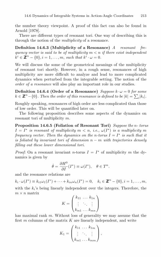
14.6 Dynamics of Integrable Systems in Action-Angle Coordinates 213
the number theory viewpoint. A proof of this fact can also be found inArnold [1978].
There are different types of resonant tori. One way of describing this isthrough the notion of the multiplicity of a resonance.
Definition 14.6.3 (Multiplicity of a Resonance) A resonant fre-
quency vector is said to be of multiplicity m < n if there exist independent
ki ∈ ZZn − 0, i = 1, . . . , m, such that ki · ω = 0.
We will discuss the some of the geometrical meanings of the multiplicityof resonant tori shortly. However, in a rough sense, resonances of highmultiplicity are more difficult to analyze and lead to more complicateddynamics when perturbed from the integrable setting. The notion of theorder of a resonance will also play an important role in our studies.
Definition 14.6.4 (Order of a Resonance) Suppose k ·ω = 0 for some
k ∈ ZZn−0. Then the order of this resonance is defined to be |k| =∑
i|ki|.Roughly speaking, resonances of high order are less complicated than thoseof low order. This will be quantified later on.
The following proposition describes some aspects of the dynamics onresonant tori of multiplicity m.
Proposition 14.6.5 (Foliation of Resonant Tori) Suppose the n- torus
I = I∗ is resonant of multiplicity m < n, i.e., ω(I∗) is a multiplicity mfrequency vector. Then the dynamics on the n-torus I = I∗ is such that it
is foliated by invariant tori of dimension n − m with trajectories densely
filling out these lower dimensional tori.
Proof: On a resonant invariant n-torus I = I∗ of multiplicity m the dy-namics is given by
θ =∂H0
∂I(I∗) ≡ ω(I∗), θ ∈ Tn.
and the resonance relations are
ki ·ω(I∗) ≡ ki1ω1(I∗) + · · ·+ kinωn(I∗) = 0, ki ∈ ZZn−0, i = 1, . . . , m,
with the ki’s being linearly independent over the integers. Therefore, them× n matrix
K =
k11 . . . k1n
.... . .
...km1 . . . kmn
has maximal rank m. Without loss of generality we may assume that thefirst m columns of the matrix K are linearly independent, and write
K1 =
k11 . . . k1m
.... . .
...km1 . . . kmm
,
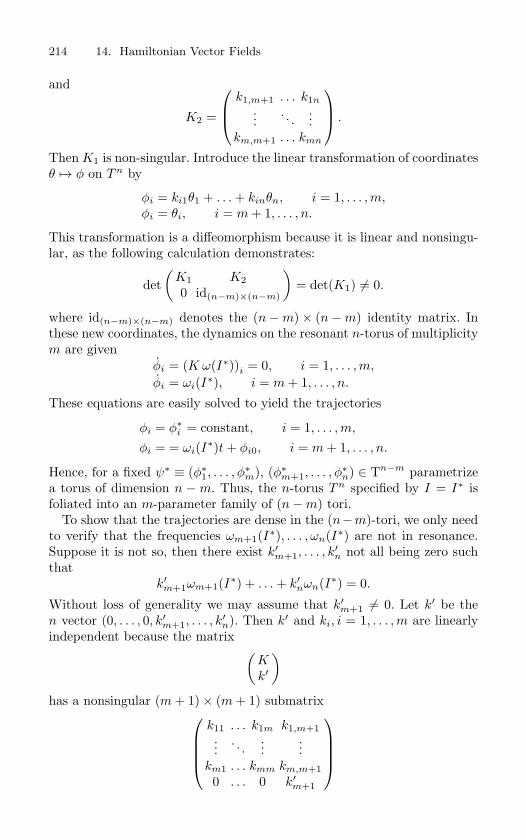
214 14. Hamiltonian Vector Fields
and
K2 =
k1,m+1 . . . k1n
.... . .
...km,m+1 . . . kmn
.
Then K1 is non-singular. Introduce the linear transformation of coordinatesθ → φ on Tn by
φi = ki1θ1 + . . . + kinθn, i = 1, . . . , m,φi = θi, i = m + 1, . . . , n.
This transformation is a diffeomorphism because it is linear and nonsingu-lar, as the following calculation demonstrates:
det(
K1 K20 id(n−m)×(n−m)
)= det(K1) = 0.
where id(n−m)×(n−m) denotes the (n−m)× (n−m) identity matrix. Inthese new coordinates, the dynamics on the resonant n-torus of multiplicitym are given
φi = (K ω(I∗))i = 0, i = 1, . . . , m,
φi = ωi(I∗), i = m + 1, . . . , n.
These equations are easily solved to yield the trajectories
φi = φ∗i = constant, i = 1, . . . , m,
φi = = ωi(I∗)t + φi0, i = m + 1, . . . , n.
Hence, for a fixed ψ∗ ≡ (φ∗1, . . . , φ
∗m), (φ∗
m+1, . . . , φ∗n) ∈ Tn−m parametrize
a torus of dimension n −m. Thus, the n-torus Tn specified by I = I∗ isfoliated into an m-parameter family of (n−m) tori.
To show that the trajectories are dense in the (n−m)-tori, we only needto verify that the frequencies ωm+1(I∗), . . . , ωn(I∗) are not in resonance.Suppose it is not so, then there exist k′
m+1, . . . , k′n not all being zero such
thatk′
m+1ωm+1(I∗) + . . . + k′nωn(I∗) = 0.
Without loss of generality we may assume that k′m+1 = 0. Let k′ be the
n vector (0, . . . , 0, k′m+1, . . . , k
′n). Then k′ and ki, i = 1, . . . , m are linearly
independent because the matrix (Kk′
)has a nonsingular (m + 1)× (m + 1) submatrix
k11 . . . k1m k1,m+1...
. . ....
...km1 . . . kmm km,m+10 . . . 0 k′
m+1
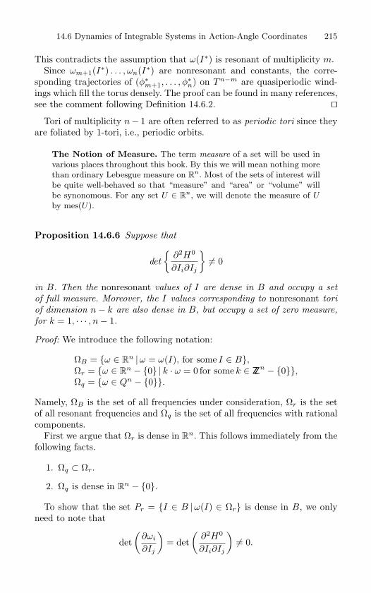
14.6 Dynamics of Integrable Systems in Action-Angle Coordinates 215
This contradicts the assumption that ω(I∗) is resonant of multiplicity m.Since ωm+1(I∗) . . . , ωn(I∗) are nonresonant and constants, the corre-
sponding trajectories of (φ∗m+1, . . . , φ
∗n) on Tn−m are quasiperiodic wind-
ings which fill the torus densely. The proof can be found in many references,see the comment following Definition 14.6.2.
Tori of multiplicity n− 1 are often referred to as periodic tori since theyare foliated by 1-tori, i.e., periodic orbits.
The Notion of Measure. The term measure of a set will be used in
various places throughout this book. By this we will mean nothing more
than ordinary Lebesgue measure on Rn. Most of the sets of interest will
be quite well-behaved so that “measure” and “area” or “volume” will
be synonomous. For any set U ∈ Rn, we will denote the measure of Uby mes(U).
Proposition 14.6.6 Suppose that
det
∂2H0
∂Ii∂Ij
= 0
in B. Then the nonresonant values of I are dense in B and occupy a set
of full measure. Moreover, the I values corresponding to nonresonant tori
of dimension n− k are also dense in B, but occupy a set of zero measure,
for k = 1, · · · , n− 1.
Proof: We introduce the following notation:
ΩB = ω ∈ Rn |ω = ω(I), for some I ∈ B,
Ωr = ω ∈ Rn − 0 | k · ω = 0 for some k ∈ ZZn − 0,
Ωq = ω ∈ Qn − 0.
Namely, ΩB is the set of all frequencies under consideration, Ωr is the setof all resonant frequencies and Ωq is the set of all frequencies with rationalcomponents.
First we argue that Ωr is dense in Rn. This follows immediately from the
following facts.
1. Ωq ⊂ Ωr.
2. Ωq is dense in Rn − 0.
To show that the set Pr = I ∈ B |ω(I) ∈ Ωr is dense in B, we onlyneed to note that
det(
∂ωi
∂Ij
)= det
(∂2H0
∂Ii∂Ij
) = 0.
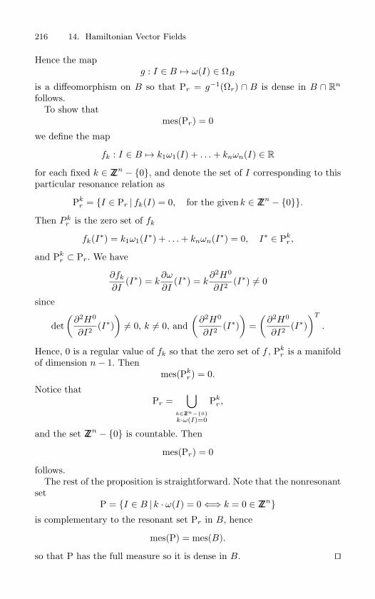
216 14. Hamiltonian Vector Fields
Hence the mapg : I ∈ B → ω(I) ∈ ΩB
is a diffeomorphism on B so that Pr = g−1(Ωr) ∩ B is dense in B ∩ Rn
follows.To show that
mes(Pr) = 0
we define the map
fk : I ∈ B → k1ω1(I) + . . . + knωn(I) ∈ R
for each fixed k ∈ ZZn − 0, and denote the set of I corresponding to thisparticular resonance relation as
Pkr = I ∈ Pr | fk(I) = 0, for the given k ∈ ZZn − 0.
Then P kr is the zero set of fk
fk(I∗) = k1ω1(I∗) + . . . + knωn(I∗) = 0, I∗ ∈ Pkr ,
and Pkr ⊂ Pr. We have
∂fk
∂I(I∗) = k
∂ω
∂I(I∗) = k
∂2H0
∂I2 (I∗) = 0
since
det(
∂2H0
∂I2 (I∗)) = 0, k = 0, and
(∂2H0
∂I2 (I∗))
=(
∂2H0
∂I2 (I∗))T
.
Hence, 0 is a regular value of fk so that the zero set of f , Pkr is a manifold
of dimension n− 1. Thenmes(Pk
r ) = 0.
Notice thatPr =
⋃k∈ZZn−0k·ω(I)=0
Pkr ,
and the set ZZn − 0 is countable. Then
mes(Pr) = 0
follows.The rest of the proposition is straightforward. Note that the nonresonant
setP = I ∈ B | k · ω(I) = 0 ⇐⇒ k = 0 ∈ ZZn
is complementary to the resonant set Pr in B, hence
mes(P) = mes(B).
so that P has the full measure so it is dense in B.
14.6 Dynamics of Integrable Systems in Action-Angle Coordinates 217
14.6b Diophantine FrequenciesCertain nonresonant frequencies play an important role in the proof of theKAM theorem. These are the diophantine frequencies, which we now define.For τ , γ > 0
Ω(τ, γ) ≡ω ∈ R
n | |ω · k| ≥ γ|k|−τ ∀k ∈ ZZn − 0
(14.6.5)
where|k| ≡ sup
i|ki|,
and we setΩ(τ) ≡
⋃γ>0
Ω(τ, γ).
It is important to note that the frequencies satisfying (14.6.5) satisfy acountable infinity of inequalities. These inequalities quantify the character-istic of these frequencies not being close to resonance.
The following proposition is classical. All pieces of the proof can be foundin Cassels [1957], Schmidt [1980], Arnold [1963], Russmann [1975], andLochak and Meunier [1988]. For completeness, we provide a few additionaldetails.
Proposition 14.6.7
1. For 0 < τ < n− 1, Ω(τ) = ∅.
2. For τ = n− 1, Ω(τ) has Lebesgue measure zero.
3. For τ > n − 1, Rn − Ω(τ) has Lebesgue measure zero, and more
precisely
mes (Rn − Ω(τ, γ)) ∩BR ≤ C(τ)γRn−1,
where BR denotes the ball of radius R in Rn.
Proof:
Proof of 1. The proof of 1 relies on the following result that we statewithout proof.
Theorem 14.6.8 (Dirichlet’s Theorem, Cassels) [1957], pg. 14
For any θ ≡ (θ1, · · · , θm) ∈ Rm the inequality
‖ p · θ ‖≡‖ p1θ1 + · · ·+ pmθm ‖< |p|−m
is satisfied by infinitely many p ∈ ZZm, where the notation ‖ · ‖ is defined
by
∀θ ∈ R, ‖ θ ‖≡ infq∈ZZ
|θ − q|. (14.6.6)
218 14. Hamiltonian Vector Fields
Without loss of generality we can assume ωn = 0. We set θi ≡ ωi
ωn, i =
1, · · · , n− 1. Then, applying Dirichlet’s theorem, for any(
ω1ωn
, · · · , ωn−1ωn
)∈
Rn−1 the inequality
‖ k1ω1
ωn+ · · ·+ kn−1
ωn−1
ωn‖< |k|−(n−1), (14.6.7)
is satisfied by infinitely many k ≡ (k1, · · · , kn−1) ∈ ZZn−1. This implies that(14.6.7) has solutions for arbitrarily large |k|.
Now we are interested in solutions of the following inequality (viewing(ω1, · · · , ωn) as given)
‖ k1ω1
ωn+ · · ·+ kn−1
ωn−1
ωn‖> γ|k|−τ , 0 < τ < n− 1. (14.6.8)
Then, for a given (ω1, · · · , ωn), simultaneous solution of (14.6.7) and(14.6.8) implies
0 < γ|k|−τ <‖ k1ω1
ωn+ · · ·+ kn−1
ωn−1
ωn‖< |k|(n−1),
or
γ <‖ k1
ω1ωn
+ · · ·+ kn−1ωn−1ωn
‖|k|−τ
< |k|−n+1+τ . (14.6.9)
Now for fixed γ > 0 the right-hand-side of this bound can be made smallerthan the left-hand-side for sufficiently large |k|, provided 0 < τ < n − 1.Hence, we conclude that for any 0 < τ < n−1, and for any
(ω1ωn
, · · · , ωn−1ωn
)the inequality
‖ k1ω1
ωn+ · · ·+ kn−1
ωn−1
ωn‖> γ|k|−τ , (14.6.10)
does not hold for all k ∈ ZZn−1.From (14.6.6) we have
|k1ω1
ωn+ · · ·+ kn−1
ωn−1
ωn+ kn| > min
kn∈ZZ|k1
ω1
ωn+ · · ·+ kn−1
ωn−1
ωn+ kn|
≡ ‖ k1ω1
ωn+ · · ·+ kn−1
ωn−1
ωn‖> γ|k|−τ ,
k ∈ ZZn−1. (14.6.11)
Now recall |k| ≡ max |ki|, and for k = 0 |k| ≥ 1. Then if we define
kn−1 ≡ (k1, · · · , kn−1) ,
andkn ≡ (k1, · · · , kn) ,
where the first n− 1 elements of kn are the same as kn−1, we have
|kn| ≥ |kn−1|,
14.6 Dynamics of Integrable Systems in Action-Angle Coordinates 219
and, thus,|kn−1|−τ ≥ |kn|−τ .
Using this fact, along with (14.6.11), we conclude that the inequality
|k1ω1 + · · ·+ kn−1ωn−1 + knωn| > ωnγ|k|−τ , k ∈ ZZn, 0 < τ < n− 1,(14.6.12)
is not solved for all k ∈ ZZn. We have shown that Ω (τ, ωnγ) = ∅ for anyγ, ωn = 0.
Proof of 2. This is the difficult case, and the reader is referred to Schmidt[1980].
Proof of 3. Here we follow Arnold [1963] and Lochak and Meunier [1988].ω · k = 0 is a resonant plane passing through the origin in R
n (and theinteger vector k is perpendicular to the plane). A neighborhood of thisplane is given by
ω ∈ Rn | |ω · k| ≤ γ|k|−τ
, (14.6.13)
and the width of this neighborhood is given by
2γ|k|−τ−1.
It is only in these neighborhoods of the resonant planes that the inequality
|ω · k| > γ|k|−τ ,
does not hold. The volume of one of these neighborhoods is given by
mes
ω ∈ Rn | |ω · k| ≤ γ|k|−τ
∩BR
= 2CγRn−1|k|τ−1, (14.6.14)
where C is a constant depending on BR. Hence we have
mes (Rn − Ω(τ, γ)) ∩BR = 2CγRn−1∑
k∈ZZn−0|k|−τ−1
≡ C(τ)γRn−1 (14.6.15)
which goes to zero as γ → 0 and where
C(τ) ≡ 2C∑
k∈ZZn−0|k|−τ−1.
This sum converges only if τ > n− 1, we leave the details of this last factto the reader.
220 14. Hamiltonian Vector Fields
14.6c Geometry of the ResonancesHere we describe a few features associated with the geometry of resonances.Essentially, these amount to properties of the equation(s)
k · ω(I) = 0, k ∈ ZZn − 0.
We can view these properties as manifested either in action space or fre-
quency space by use of the frequency map
I → ω(I), I ∈ B. (14.6.16)
Action Space
In action space we make the following observations.
• The solutions of the equation k · ω(I) = 0, k fixed, generically forma hypersurface in B.
• The solutions of the r < n equations ki · ω(I) = 0, i = 1, . . . , r,generically form a surface of codimension r in B.
We also easily conclude that resonances are nested – a resonance of mul-tiplicity r is contained in a resonance of multiplicity r − 1.
Frequency Space
In frequency space the equation(s) k · ω = 0 represent a system of linearequations. It is natural to leave out the explicit dependence of ω on I inthis representation.
Energy Conservation
In frequency space the resonance relation restricted to H0(I) = h = con-stant can be written as
k1ω1
ωn+ . . . + kn−1
ωn−1
ωn+ kn = 0
where we suppose (without loss of generality) ωn(I) does not vanish in theregion of interest.
Resonance Structure Versus the Number of Angles
n=1 In this case resonance implies ω = 0.
n=2 In this case the resonance relation restricted to the energy surface isgiven by
k1ω1
ω2+ k2 = 0.
14.7 Perturbations of Integrable Systems in Action-Angle Coordinates 221
Thus the resonances occur at isolated points in ω1ω2
space. Moreover, fornondegenerate systems they have different energies (i.e., different valuesfor the Hamiltonian). We say that for two degree-of-freedom systems theresonances are energetically isolated.
n=3 In this case the resonance relation restricted to the energy surface isgiven by
k1ω1
ω3+ k2
ω2
ω3+ k3 = 0.
The resonance relation defines lines in ω1ω3− ω2
ω3space. For a fixed (k1, k2, k3)
the line corresponds to a multiplicity one resonance. Generically, if twolines intersect they do so in an isolated point. Such a point corresponds toa multiplicity two resonance. As (k1, k2, k3) runs through ZZ3 the resultinglines are dense in ω1
ω3− ω2
ω3space. This is a significant difference between
two degree-of-freedom systems and systems with three or more degrees-of-freedom. In the former case the resonances are (generically) energeticallyisolated. In the latter case they are not.
14.7 Perturbations of Completely IntegrableHamiltonian Systems in Action-AngleCoordinates
This is a huge area, a good up-to-date and general reference is Arnold etal. [1988]. However, the two most important theorems are those due toKolmogorov [1954]-Arnold [1963] -Moser [1962] (KAM) and Nekhoroshev.Here we state them. The Hamiltonian we consider is of the form
H(I, θ) = H0(I) + εH1(I, θ), (I, θ) ∈ B × Tn. (14.7.1)
Below is the statement of the KAM theorem due to Poschel [1982].
Theorem 14.7.1 (KAM) Let the integrable Hamiltonian H0 be real an-
alytic and nondegenerate, and let the perturbed Hamiltonian H = H0+εH1
be of class Cr with r > 2n. Then, for sufficiently small ε proportional to
γ2, the perturbed system possesses smooth invariant n-tori with linear flow
for all ω ∈ Ω(n, γ), i.e., restricted to the invariant n-tori, the vector field
is analytically conjugate to φ = ω.
What about the lower dimensional tori described in Proposition 14.6.5?Recent results of Eliasson [1988], and Poschel [1989] prove the persistenceof lower-dimensional “elliptic” tori, and results of de la Llave and Wayne[1990], and Treschev [1991] prove the persistence of lower-dimensional “hy-perbolic” (or “whiskered”) tori.
The following theorem is originally due to Nekhoroshev [1977], but ithas recently been sharpened considerably in the work of Lochak [1992],
222 14. Hamiltonian Vector Fields
Lochak and Neishtadt [1992], and Poschel [1993]. It is a result that requiresanalyticity of the Hamiltonian, as well as either convexity or quasiconvexityof the unperturbed Hamiltonian.
The function H0(I) is said to be convex if
‖ ∇2H0(I)v ‖≤ M ‖ v ‖, ∇2H0
(I)v · v ≥ m ‖ v ‖2, ∀I ∈ B, v ∈ Rn,
and where 0 < m ≤ M . Quasiconvexity is convexity restricted to the
level set of the Hamiltonian.
Theorem 14.7.2 (Nekhoroshev) For any initial condition (I(0), θ(0))one has
|I(t)− I(0)| ≤ C1εb for |t| ≤ C2exp(C3ε
−a) ,
where a = b = 1/2n, C1, C2, and C3 are constants, and provided ε is small
enough.
14.8 Stability of Elliptic Equilibria
Suppose (14.0.1) has an equilibrium point, which without loss of generality,we can assume to be at (q, p) = (0, 0). We are interested in the stabilityof the equilibrium. Therefore, as a first step, we linearize (14.0.1) aboutthe equilibrium and examine the eigenvalues of the matrix associated withthe equilibrium. This matrix is an infinitesimally symplectic matrix and soProposition 14.3.5 describes the nature of the eigenvalues. If all eigenvalueslie on the imaginary axis, but none are zero, then the equilibrium is saidto be an elliptic equilibrium. Morse theory can be used to prove Liapunovstability of a large class of elliptic equilibria. We begin by developing thenecessary background to prove this result.
Definition 14.8.1 (Nondegenerate Critical Point) Suppose
F : Rn → R is a Cr, r ≥ 3, or analytic function. Suppose x = x0
is a point such that ∂F∂x (x0) = 0. Then x0 is said to be a critical point.
If x0 is such that det ∂2F∂x2 (x0) = 0 then it is said to be a nondegenerate
critical point.
Definition 14.8.2 (Morse Function) If x = x0 is a nondegenerate crit-
ical point of F (x) then F (x) is said to be a Morse function in a neighborhood
of x0.
Suppose we Taylor expand F (x) about x = 0. The n×n matrix associatedwith the second derivatives is symmetric. Therefore it can always be diag-onalized by a linear transformation. We assume that this has been done,after which the Taylor expansion assumes the form
F (x) = F (0)− c1x21 − · · · − ckx2
k + ck+1x2k+1 + · · ·+ cnx2
n +O(3),
14.9 Discrete-Time Hamiltonian Dynamical Systems 223
where ci ≥ 0, i = 1, . . . , n. The integer k is called the index of the critical
point. Then we have the following Morse lemma.
Lemma 14.8.3 (Morse) If F is a Cr, r ≥ 3, or analytic Morse function
near x = 0, then in a neighborhood of x = 0 there exists a Cr−2, or analytic
diffeomorphism, which transforms F to the form
G(x) = G(0)− y21 − · · · − y2
k + y2k+1 + · · ·+ y2
n.
Proof: See Golubitsky and Marsden [1983]. One now should be able to guess how these results are used to study sta-
bility of elliptic equilibria in Hamiltonian systems. At an elliptic equilibriumthe Hamiltonian is a Morse function. Now suppose the matrix associatedwith the second derivative of the Hamiltonian, evaluated at the equilibriumpoint, is positive definite. Then the equilibrium point has index zero andthe Hamiltonian is locally conjugate to a Hamiltonian of the form
H(q, p)−H(0, 0) = q21 + · · ·+ q2
n + p21 + · · ·+ p2
n.
Hence the energy surfaces are locally diffeomorphic to a family of spheresthat shrink down to the point (0, 0) as H → H(0, 0). Since the trajectoriesare tangent to the energy surfaces Liapunov stability follows. In the casethat the matrix associated with the second derivative of the Hamiltonian,evaluated at the equilibrium point, is negative definite we apply the samereasoning to the time reversed vector field (i.e., let H → −H) and obtainthe same result.
14.9 Discrete-Time Hamiltonian DynamicalSystems: Iteration of Symplectic Maps
The dynamics of symplectic maps can be viewed as a discrete time ana-log of the dynamics generated by Hamiltonian vector fields. Proposition14.3.2 gives us information about linearized stability of periodic orbits ofsymplectic maps and, hence, the local invariant manifold structure (i.e.existence and dimensions of stable, unstable, and center manifolds of pe-riodic orbits). There are also discrete analogs of the KAM theorem andNekoroshev’s theorem, which we now describe.
14.9a The KAM Theorem and Nekhoroshev’sTheorem for Symplectic Maps
As in the continuous time case, the setting for these theorems is that ofperturbations of integrable symplectic maps. Before stating the results wemust develop the appropriate setting.
224 14. Hamiltonian Vector Fields
Let Bδ denote the open ball in Rn of radius δ. Then the 2n-dimensional
annulus is denoted by Aδ = Bδ × Tn. We define the following map on Aδ:
f0 : Aδ → Aδ
(I, θ) → (I, θ + ω(I)) = f0(I, θ). (14.9.1)(14.9.2)
It should be clear that Aδ is foliated by an n-parameter family of invariantn-tori. We assume that ω is given by the gradient of a function, i.e.,
ω = ∇h.
In this case f0 is a globally symplectic map with generating function h.Now we want to consider perturbations of f0, but not just any perturba-
tions. Rather, we only wish to consider perturbations where the resultingperturbed map is also symplectic. This can be achieved through the useof generating functions, for which we refer the reader to Whittaker [1904],Goldstein [1980], Abraham and Marsden [1978], Arnold [1978], or Section13.7c for more background. For our limited purposes one could just takethe following as the definition of the maps under consideration.
We consider the map generated by a perturbation of h:
Σ(I ′, θ) = h(I ′) + σ(I ′, θ),
where σ is small, with ‖ σ ‖≡ ε. Then the perturbed map f : Aδ → Aδ isimplicitly defined by
f : Aδ → Aδ,
(I ′, θ′) =(
I − ∂σ
∂θ, θ + ω(I ′) +
∂σ
∂I ′
), (14.9.3)
where primes denote the image of the respective coordinate under the map.
Nekhoroshev Theorem for Symplectic Maps
The discrete version of Nekhoroshev’s theorem was first announced inNekhoroshev [1977]. Details first appeared in Kuksin and Poschel [1994],but see also Bazzani et al. [1990] and Lochak [1992]. We first establishsome notation. Let fs(I, θ) ≡ (Is, θs), with (I0, θ0) ≡ (I, θ). We assumethat (Is, θs) remains in Aδ for all times under consideration.
Theorem 14.9.1 Suppose h and σ are analytic and h is a convex function.
If ε ≡‖ σ ‖≤ ε0, then ‖ Is − I ‖≤ cεb when |s| ≤ c exp (ε−a), s ∈ ZZ, and
where a = b = 12n+2 .
Proof: See Kuksin and Poschel [1994].
14.10 Generic Properties of Hamiltonian Dynamical Systems 225
KAM Theorem for Symplectic Maps
The discrete version of the KAM theorem was first worked out in theanalytic setting by Douady [1982] (although the two dimensional Mosertwist theorem in the finitely differentiable case was obtained much earlier).Kuksin and Poschel [1994] provide a new proof. First we establish somenotation.
We assume that the unperturbed map is nondegenerate in the followingsense:
det∇2h(I) = det∂ω
∂I = 0.
This condition is often referred to as the twist condition. We are concernedwith the preservation tori whose unperturbed frequency vectors satisfy thefollowing diophantine condition:
|2πp + q1ω1 + · · ·+ qnωn| > c (|q1|+ · · ·+ |qn|)−γ, (14.9.4)
for all q ∈ ZZn − 0 and p ∈ ZZ, and where c > 0 and γ > n are constants.
Theorem 14.9.2 For analytic f , and for ε sufficiently small, the perturbed
map f possesses analytic invariant n-tori for all ω satisfying (14.9.4).
Moreover, the dynamics restricted to the invariant n-tori is analytically
conjugate to the rigid rotation φ → φ + ω.
Proof: See Kuksin and Poschel [1994].
14.10 Generic Properties of HamiltonianDynamical Systems
The special structure of Hamiltonian dynamical systems (both continuousand discrete time) give rise to additional generic properties than thosedescribed in the usual Kupka-Smale theorems discussed in Chapter 12.The classic papers on this subject are Robinson [1970a, b], Takens [1970],[1972], Newhouse [1977], and Pugh and Robinson [1983]. Here we contentourselves with just stating a few of these properties, which we will expandupon when we learn more about global dynamics later in the book.
For C1 Hamiltonian systems the following properties are generic (in thesense of holding for a residual subset in the appropriate “space of dynamicalsystems”).
Hyperbolic periodic orbits are dense in the phase space (Pugh and Robin-son [1983]).
Every hyperbolic periodic orbit has a transverse homoclinic point in anyneighborhood of any point in the phase space (Taken [1970], [1972],Newhouse [1977]).
226 14. Hamiltonian Vector Fields
The reader should take great care in applying these generic results tospecific dynamical systems following the caveats described in Chapter 12.In a measure theoretic sense, residual sets can be “small”. Herman [1991]has constructed an explicit example of a Hamiltonian system with no peri-odic orbits. Another important point for applications is that “generic typetheorems” are typically proved in a Cr setting. In many applications thedynamical systems are analytic. The Cr techniques generally make theresults inapplicable in an analytic setting.
14.11 Exercises1. Prove that 〈·, J·〉 is a symplectic form on R
2n.
2. Suppose a 2n × 2n matrix of real numbers A satisfies
AT
JA = J,
where A has the form (a bc d
),
and a, b, c, d are n × n matrices. Show that
(a) The n × n matrices aT c and bT d are symmetric,
(b) aT d − cT b = id,
(c) detA = 1.
3. Prove that the composition of two symplectic transformations is a symplectic trans-formation.
4. Consider a (real), canonical autonomous Hamiltonian vector field having an equilib-rium point.
(a) Can the equilibrium point be asymptotically stable?
(b) Can the equilibrium point have an odd dimensional center manifold?
5. Consider a (real), symplectic map having a periodic orbit.
(a) Can the periodic orbit be asymptotically stable?
(b) Can the periodic orbit have an odd dimensional center manifold?
6. Prove that the flow generated by a Hamiltonian vector field is volume preserving.
7. Prove that symplectic maps preserve volume.
8. Prove that two dimensional volume preserving vector fields are Hamiltonian.
9. Construct an example of a vector field in dimension 2n, n ≥ 2, that is volume preserv-ing but not Hamiltonian.
10. Consider a Hamiltonian vector field in the plane having a hyperbolic equlibrium pointconnected to itself by a homoclinic orbit. Is the homoclinic orbit structurally stable?Consider a heteroclinic connection between two hyperbolic equlibrium points. Is thissituation structurally stable? Do the results change if the equilibria are not hyperbolic?Do the results hold in higher dimensions?
14.11 Exercises 227
11. Consider the following vector field in complex coordinates zz = x1+iy1, z2 = x2+iy2:
z1 = i[−(σ − β)z1 + ∆z1 + π1z21 z1 + π2z1z2z2 + π3z1z
22 ],
z2 = i[−(σ + β)z2 + ∆z2 + π1z22 z2 + π2z1z2z1 + π3z2z
21 ].
This equation is a normal form that arises in the study of a variety of two degree-of-freedom parametrically forced mechanical systems (see Feng and Wiggins [1993]). Theparameters represent
• σ – difference between the forcing frequency and the sum of the two naturalfrequencies.
• β – difference between the two natural frequencies.
• ∆ – amplitude of the sinusoidal excitation.
• π1, π2, π3–coefficients of the nonlinear terms depending on the mode numbersand geometrical properties.
(a) Show that this vector field is Hamiltonian.
(b) Show that through rescaling we can set
∆ = 1, π1 = −1,
and that it the rescaled cartesian coordinates the vector field is given by
x1 = (σ − π1E + 1)y1 − 2π3Lx2 − βy1 + Cy1(x22 + y
22)
y1 = (−σ + π1E + 1)x1 − 2π3Ly2 + βx1 − Cx1(x22 + y
22)
x2 = (σ − π1E + 1)y2 + 2π3Lx1 + βy2 + Cy2(x21 + y
21)
y2 = (−σ + π1E + 1)x2 + 2π3Ly1 − βx2 − Cx2(x21 + y
21)
(14.11.1)
whereE = x
21 + y
21 + x
22 + y
22 ,
L = x1y2 − x2y1,
C = π1 − π2 − π3.
The parameters are now reduced to
d, σ, β, C, π3.
(c) Show that (14.11.1) is Hamiltonian with Hamiltonian given by
H =σ
2E +
14
E2 + π3L
2 +12(y2
1 + y22 − x
21 − x
22)
+β
2(x2
2 + y22 − x
21 − y
21) +
C
2(x2
1 + y21)(x2
2 + y22).
(d) Consider the transformation
x1 = q1 cos q2,
x2 = q1 sin q2,
y1 = p1 cos q2 − p2q−11 sin q2,
y2 = p1 sin q2 + p2q−11 cos q2, (14.11.2)
228 14. Hamiltonian Vector Fields
with inverse
q1 =√
x21 + x2
2,
p1 =x1y1 + x2y2√
x21 + x2
2
,
q2 = tan−1 x2
x1,
p2 = x1y2 − x2y1. (14.11.3)
Show that this transformation is canonical.
(e) Show that in this new coordinate system the vector field is Hamiltonian withHamiltonian given by
H ≡ H0 + εH1 =σ
2E +
14
E2 + π3p
22 +
12(p2
1 + p22q
−21 − q
21)
+(
β
2D +
C
8(E2 − D
2))
(14.11.4)
whereE = q
21 + p
21 + p
22q
−21 ,
D = 2p1p2q−11 sin 2q2 + (p2
2q−21 − q
21 − p
21) cos 2q2.
(f) Show that for β = C = 0 this system is completely integrable.
12. Consider the following two degree-of-freedom system in complex coordinates
−ic + (12
|c|2 +12
|b|2 − 1)c +12(cb + bc)b = 0,
−ib + (12
|c|2 +34
|b|2 − (1 + k2))b +
12(cb + bc)c = 0,
where k is a real parameter. This equation arises in the study of a two-mode truncationof the nonlinear Schrodinger equation, see Bishop et al. [1990] and Kovacic and Wiggins[1992].
(a) Show that this system is Hamiltonian.
(b) Show that the coordinate transformation
c = |c|eiθ, b = (x + iy)eiθ
,
is canonical, and be careful to describe where it is defined.
(c) Show that in these new coordinates the vector field takes the form
x = −k2y − 3
4x2y +
14
y3,
y = (k2 − 2I)x +74
x3 +
34
xy2,
I = 0,
θ = 1 − I − x2, (14.11.5)
and it is Hamiltonian with Hamiltonian given by
H =12
I2 − I − 7
16x4 − 3
8x2y2 +
116
y4 + (I − 1
2k2)x2 − 1
2k2y2. (14.11.6)
(d) Show that the system is completely integrable.
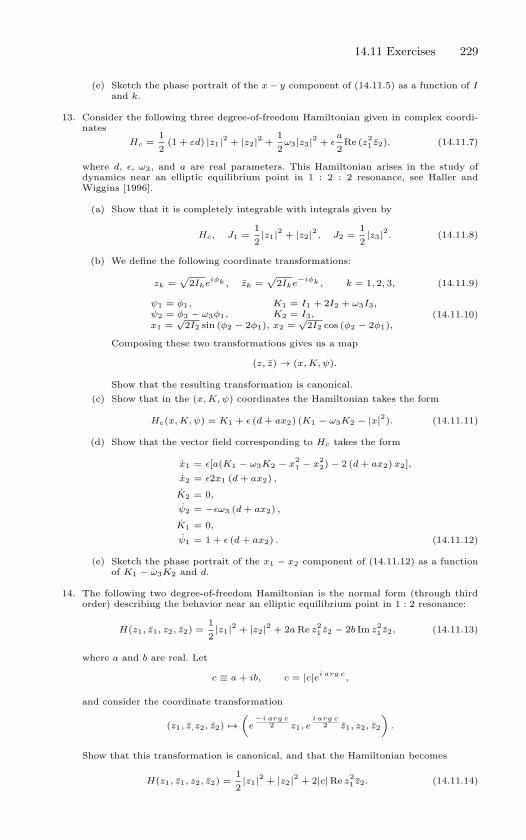
14.11 Exercises 229
(e) Sketch the phase portrait of the x − y component of (14.11.5) as a function of Iand k.
13. Consider the following three degree-of-freedom Hamiltonian given in complex coordi-nates
Hc =12
(1 + εd) |z1|2 + |z2|2 +12
ω3|z3|2 + εa
2Re (z2
1 z2). (14.11.7)
where d, ε, ω3, and a are real parameters. This Hamiltonian arises in the study ofdynamics near an elliptic equilibrium point in 1 : 2 : 2 resonance, see Haller andWiggins [1996].
(a) Show that it is completely integrable with integrals given by
Hc, J1 =12
|z1|2 + |z2|2, J2 =12
|z3|2. (14.11.8)
(b) We define the following coordinate transformations:
zk =√
2Ikeiφk , zk =
√2Ike
−iφk , k = 1, 2, 3, (14.11.9)
ψ1 = φ1, K1 = I1 + 2I2 + ω3I3,ψ2 = φ3 − ω3φ1, K2 = I3,x1 =
√2I2 sin (φ2 − 2φ1), x2 =
√2I2 cos (φ2 − 2φ1),
(14.11.10)
Composing these two transformations gives us a map
(z, z) → (x, K, ψ).
Show that the resulting transformation is canonical.
(c) Show that in the (x, K, ψ) coordinates the Hamiltonian takes the form
Hc(x, K, ψ) = K1 + ε (d + ax2) (K1 − ω3K2 − |x|2). (14.11.11)
(d) Show that the vector field corresponding to Hc takes the form
x1 = ε[a(K1 − ω3K2 − x21 − x
22) − 2 (d + ax2) x2],
x2 = ε2x1 (d + ax2) ,
K2 = 0,
ψ2 = −εω3 (d + ax2) ,
K1 = 0,
ψ1 = 1 + ε (d + ax2) . (14.11.12)
(e) Sketch the phase portrait of the x1 − x2 component of (14.11.12) as a functionof K1 − ω3K2 and d.
14. The following two degree-of-freedom Hamiltonian is the normal form (through thirdorder) describing the behavior near an elliptic equilibrium point in 1 : 2 resonance:
H(z1, z1, z2, z2) =12
|z1|2 + |z2|2 + 2a Re z21 z2 − 2b Im z
21 z2, (14.11.13)
where a and b are real. Let
c ≡ a + ib, c = |c|ei arg c,
and consider the coordinate transformation
(z1, z,z2, z2) →(
e−i arg c
2 z1, ei arg c
2 z1, z2, z2
).
Show that this transformation is canonical, and that the Hamiltonian becomes
H(z1, z1, z2, z2) =12
|z1|2 + |z2|2 + 2|c| Re z21 z2. (14.11.14)

230 14. Hamiltonian Vector Fields
15. Show that the Poincare map constructed in section 10.4 is symplectic.
16. Consider the following frequency vectors
(a) ω = 0.
(b) ω = 1.
(c) ω = (1, 0).
(d) ω = (√
2, 0).
(e) ω = (√
2, 1).
(f) ω = (√
2, 0, 0).
(g) ω = (√
2, 0, 1).
(h) ω = (√
2, 1, 1).
(i) ω = (√
2,√
2, 1).
(j) ω = (√
2,√
2,√
2).
(k) ω = (√
2, 2, 1).
(l) ω = (1, 1, 1).
(m) ω = (1, 2, 1).
(n) ω = (1, 2, 3).
(o) ω = (1, 2, 8).
Which of these is resonant? For the the resonant frequency vectors, compute the mul-tiplicity of the resonance.
17. Compare the Liouville-Arnold Theorem (Theorem 14.5.1)with the results obtained inExercise 20 of Chapter 13.
15
Gradient Vector Fields
In this chapter we consider vector fields that are given by the gradientof a scalar valued function, which are referred to as gradient vector fields.Gradient vector fields arise in a variety of applications. For example, theyarise in the study of neural networks (Haykin [1994]) and in the study ofelectrical circuits and networks (see Hirsch and Smale [1974]).
Consider a vector field of the form
x = −∇V (x), x ∈ Rn, (15.0.1)
where V (x) is a scalar valued function on Rn that is Cr, r ≥ 2. The minus
sign in front of the gradient is traditional and imposes no restriction as wecan always redefine V (x) as −V (x). The special structure of this vectorfield, i.e., the fact that it is a gradient of a scalar valued function, imposesstrict constraints on the nature of the dynamics, as we shall see.
First, it should be clear that equilibrium points of (15.0.1) are relativeextrema of V (x). Moreover, at any point except for an equilibrium point,the vector field (15.0.1) is perpendicular to the level sets of V (x). We canget more information by differentiating V (x) along trajectories of (15.0.1),i.e.,
V (x) = ∇V (x) · x,
= ∇V (x) · (−∇V (x)) ,
= −|∇V (x)|2, (15.0.2)
where “·” is the Euclidean inner product and | · | is the induced Euclideannorm. The next result follows immediately from this calculation.
Proposition 15.0.1 V (x) ≤ 0 and V (x) = 0 if and only if x is an equi-
librium point of (15.0.1).
Using V (x) to construct an appropriate Liapunov function, we can obtainstability information about certain equilibrium points.
Proposition 15.0.2 Suppose x is an isolated minimum of V (x), i.e., there
is a neighborhood of x that contains no other minima of V (x). Then x is
an asymptotically stable equilibrium point of (15.0.1).
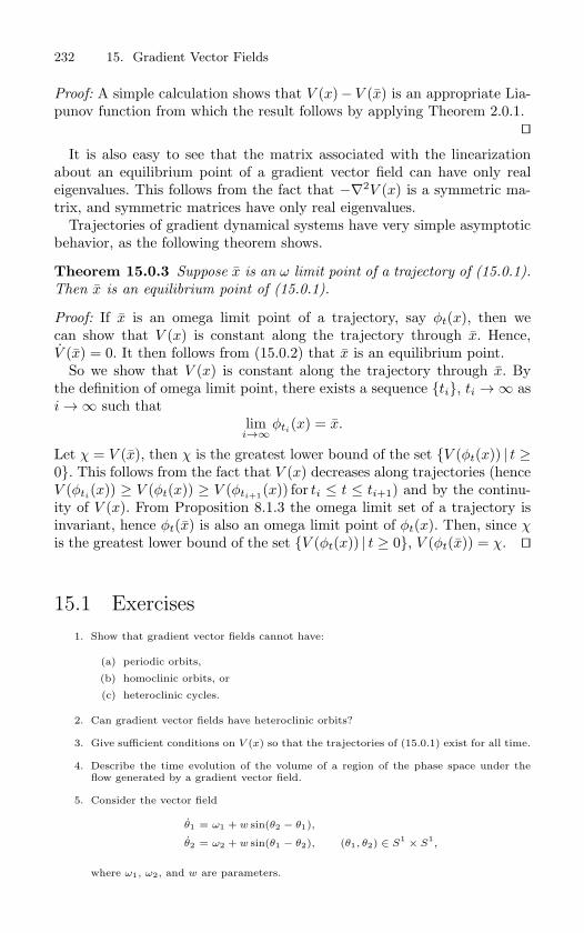
232 15. Gradient Vector Fields
Proof: A simple calculation shows that V (x)− V (x) is an appropriate Lia-punov function from which the result follows by applying Theorem 2.0.1.
It is also easy to see that the matrix associated with the linearization
about an equilibrium point of a gradient vector field can have only realeigenvalues. This follows from the fact that −∇2V (x) is a symmetric ma-trix, and symmetric matrices have only real eigenvalues.
Trajectories of gradient dynamical systems have very simple asymptoticbehavior, as the following theorem shows.
Theorem 15.0.3 Suppose x is an ω limit point of a trajectory of (15.0.1).
Then x is an equilibrium point of (15.0.1).
Proof: If x is an omega limit point of a trajectory, say φt(x), then wecan show that V (x) is constant along the trajectory through x. Hence,V (x) = 0. It then follows from (15.0.2) that x is an equilibrium point.
So we show that V (x) is constant along the trajectory through x. Bythe definition of omega limit point, there exists a sequence ti, ti →∞ asi →∞ such that
limi→∞
φti(x) = x.
Let χ = V (x), then χ is the greatest lower bound of the set V (φt(x)) | t ≥0. This follows from the fact that V (x) decreases along trajectories (henceV (φti
(x)) ≥ V (φt(x)) ≥ V (φti+1(x)) for ti ≤ t ≤ ti+1) and by the continu-ity of V (x). From Proposition 8.1.3 the omega limit set of a trajectory isinvariant, hence φt(x) is also an omega limit point of φt(x). Then, since χis the greatest lower bound of the set V (φt(x)) | t ≥ 0, V (φt(x)) = χ.
15.1 Exercises1. Show that gradient vector fields cannot have:
(a) periodic orbits,
(b) homoclinic orbits, or
(c) heteroclinic cycles.
2. Can gradient vector fields have heteroclinic orbits?
3. Give sufficient conditions on V (x) so that the trajectories of (15.0.1) exist for all time.
4. Describe the time evolution of the volume of a region of the phase space under theflow generated by a gradient vector field.
5. Consider the vector field
θ1 = ω1 + w sin(θ2 − θ1),
θ2 = ω2 + w sin(θ1 − θ2), (θ1, θ2) ∈ S1 × S
1,
where ω1, ω2, and w are parameters.
15.1 Exercises 233
(a) Show that this is a gradient vector field.
(b) Determine the phase portrait for this vector field.
(c) Can this vector field have periodic orbits? Would the existence of periodic orbitscontradict Theorem 15.0.3?
16
Reversible Dynamical Systems
In this section we introduce the notion of reversible dynamical systems.Another example of a class of dynamical systems with “special structure”that constrains the dynamics. Such systems often arise in applications (seeRoberts and Quispel [1992] for many examples, as well as the exercises atthe end of this chapter) and may have the seemingly peculiar property ofsimultaneously possessing Hamiltonian-like dynamics (e.g. KAM tori) anddissipative dynamics (e.g. attractors). We begin by defining reversibility inboth the continuous and discrete time settings. Comprehensive referencesare Sevryuk [1986], [1992], and Roberts and Quispel [1992].
16.1 The Definition of Reversible DynamicalSystems
Consider the following continuous and discrete time dynamical systems:
x = f(x), xn+1 = g(xn), x ∈ Rn,
which we assume to be Cr, r ≥ 1. Next consider a Cr map
G : Rn → R
n,
satisfyingG G = id,
where id stands for the identity map. G is called an involution. Then avector field is said to be reversible if
d
dt(G(x)) = −f(G(x)). (16.1.1)
From this definition we can see the motivation for the term reversible. Avector field, x = f(x), is reversible if the dynamics on the phase spaceG · Rn is given by the time reversed vector field. Using the chain rule onthe left hand side of (16.1.1), as well as the identity x = f(x), we seethat the definition of reversibility for a vector field reduces to the followingrelationship between G and f :
DG · f = −f G, (16.1.2)
16.2 Examples of Reversible Dynamical Systems 235
where in this section the “·” notation means ordinary matrix multiplication,with a matrix to the left of · and a vector to the right of ·.
Next we consider maps. A map is said to be reversible if
g(G(xi+1)) = G(xi). (16.1.3)
The motivation for the term reversible should be apparent. In the trans-formed phase space, G·Rn, g reverses the temporal direction of trajectories.Substituting xi+1 = g(xi) into the left hand side of (16.1.3), we obtain thefollowing relationship between G and g that is required for g to be re-versible:
g G g = G. (16.1.4)
16.2 Examples of Reversible Dynamical Systems
We now consider some explicit examples of reversible dynamical systems.
Example 16.2.1. Consider a canonical Hamiltonian vector field where the
Hamiltonian is even in the momenta, i.e.,
H(q, p) = H(q, −p), (q, p) ∈ Rn × R
n.
Hamilton’s equations are given by
q =∂H
∂p,
p = −∂H
∂q. (16.2.1)
It is easy to verify that the map
G : (q, p) → (q, −p),
is an involution of R2n and that (16.2.1) satisfies (16.1.1).
End of Example 16.2.1
Example 16.2.2. The following example is from Roberts and Quispel [1992].
Consider the vector field
x = x(1 − x), x ∈ R.
This vector field is reversible with respect to the involution
G : x → 1 − x.
Also, this vector field is not Hamiltonian, and it is not volume preserving. It has
a repelling fixed point at x = 0 and an attracting fixed point at x = 1.
End of Example 16.2.2
236 16. Reversible Dynamical Systems
16.3 Linearization of Reversible DynamicalSystems
Suppose x = x0 is a fixed point. We now consider the structure of reversibledynamical systems linearized about fixed points.
16.3a Continuous TimeLetting x = x0 + ξ, (16.1.1) becomes
d
dt(G(x0 + ξ)) = −f (G(x0 + ξ)) .
Taylor expanding each side in ξ gives
DG(x0 + ξ)(x0 + ξ
)= −f
(G(x0) + DG(x0)ξ +O(|ξ|2)
)= −f (G(x0))−Df (G(x0))DG(x0)ξ +O
(|ξ|2)
).
It follows from (1.15.2) that if x0 is a fixed point, then G(x0) is a fixedpoint, and therefore f (G(x0)) = 0. Then this relation becomes
DG(x0)ξ = −Df (G(x0))DG(x0)ξ+ O(|ξ|2) +O(|ξ||ξ|).
Note that ξ = Df(x0)ξ + O(|ξ|2). Substituting this expression into theleft-hand-side of the equation, and dropping the O(|ξ|2) terms, we obtain
DG(x0)Df(x0) = −Df (G(x0))DG(x0). (16.3.1)
Suppose G(x0) = x0. Then x0 is said to be a symmetric fixed point. Forsymmetric fixed points (16.3.1) has the form
DG(x0)Df(x0) = −Df(x0)DG(x0), (16.3.2)
and the matrix Df(x0) is said to be infinitesimally reversible. In general,we have the following definition.
Definition 16.3.1 (Infinitesimally Reversible) Suppose G : Rn → R
n
is a linear involution and A : Rn → R
n is a linear map. Then A is said to
be infinitesimally reversible if
AG + GA = 0.
Note that this linearization condition is defined at a symmetric fixed point.
16.3 Linearization of Reversible Dynamical Systems 237
Note that we have not proven that if G is an involution, so is DG. This istrue for DG evaluated at a symmetric fixed point, as can be easily verifiedwith a simple calculation using the definition of involution and the chainrule that we leave to the reader.
Sevryuk [1986], [1992] has studied the spectra of infinitesimally reversiblelinear maps. It can be shown that if λ ∈ C is an eigenvalue of an infinitesi-mally reversible linear map then so is −λ. Moreover, all nonzero eigenvaluesoccur in real pairs (x,−x), x ∈ R, purely imaginary pairs, (iy,−iy), y ∈ R,and quadruplets, ±x± iy. This is made precise in the following proposition(courtesy of Jerry Marsden).
Proposition 16.3.2 Suppose A is an n×n infinitesimally reversible linear
matrix. Then the characteristic polynomial p(λ) of A satisfies
p(−λ) = (−1)np(λ), λ ∈ C.
In particular, if λ is an eigenvalue of A so is −λ. If A is nonsingular, then
n is even. In any case, the spectrum of A is symmetric with respect to the
real and imaginary axes.
Proof: By definition 16.3.1 we have AG + GA = 0, which implies
GAG−1 = −A,
and p(λ) = det (A− λ1l), where 1l denotes the n× n identity matrix (notethat G−1 = G since G is an involution). Using these two equations, weobtain
p(λ) = det (A− λ1l)= det
(G (A− λ1l) G−1)
= det(GAG−1 − λ1l
)= det (−A− λ1l)= (−1)n det (A + λ1l)= (−1)n p(−λ).
It follows immediately that the spectrum of A is symmetric with respectto the real and imaginary axes. Moreover, if n is odd, then p is an oddfunction of λ, and so 0 is an eigenvalue. Then if n is odd, A cannot beinvertible.
Note that the proof of this proposition is identical to the proof of Propo-sition 14.3.5 which described the eigenvalues of infinitesimally symplecticmatrices.
238 16. Reversible Dynamical Systems
16.3b Discrete TimeWe carry out the same procedure for maps as we carried out for vectorfields above. Substituting x = x0 + ξ into (16.1.3)
g G(x0 + ξi+1) = G(x0 + ξi),
and Taylor expanding in ξ gives
g G(x0) + Dg(G(x0)) ·DG(x0)ξi+1 +O(|ξi+1|2)
= G(x0) + DG(x0)ξi +O(|ξi|2).
If we substitute the following expression for ξi+1 into this expression
ξi+1 = Dg(x0)ξi,
then the terms of order ξi give us the following relation:
Dg (G(x0))DG(x0)Dg(x0) = DG(x0). (16.3.3)
If x0 is a symmetric fixed point (16.3.3) becomes
Dg(x0)DG(x0)Dg(x0) = DG(x0), (16.3.4)
and the matrix Dg(x0) is said to be reversible. In general, we have thefollowing definition.
Definition 16.3.3 (Reversible) Suppose G : Rn → R
n is a linear invo-
lution and A : Rn → R
n is a linear map. Then A is said to be reversibleif
AGA = G.
Note that this linearization condition is defined at a symmetric fixed point.
Sevryuk [1986], [1992] has also studied the spectra of reversible linearmaps. It can be shown that if λ ∈ C is an eigenvalue of a reversible linearmap then so is 1
λ . Moreover, all eigenvalues different from 1 and −1 occur inreal pairs (x, 1
x ), x ∈ R, unitary pairs, (eiy, e−iy), y ∈ R, and quadruplets,x±1e±iy. We prove this in the following proposition.
Proposition 16.3.4 Suppose A : Rn → R
n is a linear operator that is
reversible with respect to the linear involution G : Rn → R
n. Then if λis an eigenvalue of A so is 1
λ , λ, and 1λ. If A does not have 1 and −1 as
eigenvalues, then n is even.
16.4 Additional Properties of Reversible Dynamical Systems 239
Proof: First, note that it follows from the relation AGA = G that detA =±1. Hence, 0 is not an eigenvalue of A. Moreover, AGA = G is equivalentto A = GA−1G, where we have used the fact that G is an involution, i.e.,G = G−1. Using these results, we have
p(λ) = det (A− λ1l),= det
(GA−1G− λ1l
),
= det(G
(A−1 − λ1l
)G),
= det(A−1 − λ1l
),
= det(A−1 (1l− λA)
),
= det A−1 det (1l− λA) ,
= ±1 det(−λ
(− 1
λ1l + A
)),
= ±1 (λ)np
(1λ
).
Hence, it immediately follows that if λ is an eigenvalue of A so is 1λ . Since
A is real, it also follows that λ and 1λ
are also eigenvalues. From this isfollows that if 1 and −1 are not eigenvalues, the eigenvalues occur in pairsor quartets. Hence n must be even.
16.4 Additional Properties of ReversibleDynamical Systems
We end this section with a few general remarks about reversible dynamicalsystems. Additional properties are developed in the exercises.
1. We saw that near symmetric fixed points the spectra of the associ-cated linearized dynamical systems is very similar to that of Hamil-tonian dynamical systems. There are many more similarities betweenreversible dynamical systems and Hamiltonian systems. An extensiveoutline, with references, can be found in Sevryuk [1991]. Most no-tably, there is a KAM theory for reversible dynamical systems (but,interestingly enough, there is no analog of Nekhoroshev’s theorem).
2. Despite the similarities between reversible and Hamiltonian dynam-ical systems, reversible dynamical systems can simultaneously dis-play non-Hamiltonian behavior (odd-dimensionality notwithstand-ing). For example, numerical simulations of dynamical systems thatdisplay KAM-type behavior, as well as possess attractors and re-pellers, can be found in Roberts and Quispel [1992] and Politi et al.[1986].
240 16. Reversible Dynamical Systems
16.5 ExercisesExercises 1-4 are examples given in the review paper of Roberts and Quispel [1992].
1. The following vector field arises in laser physics (Arecchi [1987]):
x = zx + y + C1,
y = zy − x,
z = C2 − x2 − y
2, (x, y, z) ∈ R
3,
where C1 and C2 are parameters. Prove that this is a reversible vector field. Is thevector field volume-preserving?
2. The following vector field arises in the study of non-equilibrium thermodynamics(Hoover et al. [1987]):
x = y,
y = F − ε sin x − zy,
z = α(y2 − 1), (x, y, z) ∈ R3,
where F , α, and ε are parameters. Prove that this is a reversible vector field.
3. The following vector field is an idealized model describing the sedimentation of smallparticles in a fluid (see Golubitsky et al. [1991]):
ri =n−2∑k=1
[U(ri+1 + · · · + ri+k) − U(ri−1 + · · · + ri−k)] , i = 1, . . . , n,
where
U(r) =ez
|r|+
(ez · r)r|r|3
,
the indices are taken mod n, r1, . . . , rn ∈ R3 denote the consecutive edges of an n-
sided polygon in R3, and ez is a unit vector in the z direction (in which gravity is
acting). Prove that this is a volume-preserving, reversible vector field.
4. The following vector field models a series array of Josephson junctions in parallel witha single resistor (Tsang et al. [1991]):
θk = Ω + a cos θk +1N
N∑i=1
cos θi, k = 1, . . . , N,
where θk are the phase angles (defined mod 2π), and Ω and a are parameters. Provethat this is a reversible vector field.
5. Suppose G : Rn → R
n is a Cr, r ≥ 1, involution. Prove that at a symmetric fixedpoint DG is also an involution.
6. Suppose a map g : Rn → R
n is reversible with respect to the involution G : Rn → R
n.Then show that g can be written as the product of two involutions, i.e.,
g = H G, H H = id.
7. Suppose a map g : Rn → R
n is reversible with respect to the involution G : Rn → R
n.Then show that g is invertible.
16.5 Exercises 241
8. Consider the so-called Chirikov-Taylor or Standard map:
x′ = x + y,
y′ = y +
K
2πsin 2πx
′, (x, y) ∈ R
2,
where K is a parameter. Show that it can be written as the product of two involutionsH G.
9. Consider the following area-preserving Henon map:
x′ = y,
y′ = −x + 2Cy + 2y
2, (x, y) ∈ R
2,
where C is a parameter. Show that it can be written as the product of two involutionsH G.
10. Suppose a map g : Rn → R
n is reversible with respect to the involution G : Rn → R
n.Suppose Γ ⊂ R
n is an invariant set for g, i.e., g(Γ) = Γ. Then show that G(Γ) is alsoan invariant set for g.
11. Suppose a map g : Rn → R
n is reversible with respect to the involution G : Rn →
Rn. Let x0 be a hyperbolic saddle point for g with stable and unstable manifolds
denoted W s(x0) and W u(x0), respectively. Show that G (W s(x0)) = W u (G(x0)) andG (W u(x0)) = W s (G(x0))
12. Suppose a map g : Rn → R
n is reversible with respect to the involution G : Rn → R
n.Let x0 be a hyperbolic saddle point for g with stable and unstable manifolds denotedW s(x0) and W u(x0), respectively. Let Fix(G) denote the fixed point set of G andsuppose W s(x0) intersects Fix(G). If G(x0) = x0 show that the intersection point is ahomoclinic point and if G(x0) = x0 show that the intersection point is a heteroclinicpoint.
13. Suppose a map g : Rn → R
n is reversible with respect to the involution G : Rn → R
n.Show that reversibility is preserved under conjugacy.
14. Suppose the Cr, r ≥ 1 vector field x = f(x), x ∈ Rn, is reversible with respect to
the involution G : Rn → R
n. Let φt(·) denote the flow generated by this vector field.Show that φt(·) is a one-parameter family of reversible diffeomorphisms.
15. Show that a linear map represented by a symplectic matrix is reversible.
16. Show that a linear map represented by an infinitesimally symplectic matrix is infinites-imally reversible.
17
Asymptotically AutonomousVector Fields
Imagine a system that is subjected to some type of time-dependent distur-bance that “dies away” in time. Mathematically, this might be representedby a nonautonomous vector field that becomes autonomous as time in-creases. Now many dynamical properties are only defined in the limit ast →∞. Therefore, in order to study the long time behavior of such a systemwould it be sufficient to study the long time behavior of the autonomousvector field obtained in the limit as t →∞? This is one of the questions wewill address in our discussion in this chapter of asymptotically autonomous
vector fields, which we now define more precisely.Consider the following nonautonomous vector field
x = f(x, t), x ∈ Rn, (17.0.1)
which we assume to be Cr, r ≥ 1 (this can be weakened to continuityin t, and locally Lipschitz in x). Suppose that (17.0.1) is asymptotically
autonomous in the sense that
f(x, t) → g(x), t →∞,
where the convergence is locally uniform in x ∈ Rn, i.e., convergence occurs
for any x in any compact subset of Rn. We denote the autonomous limit
equation byx = g(x), x ∈ R
n. (17.0.2)
For both (17.0.1) and (17.0.2) we assume that the trajectory through anypoint x ∈ R
n exists for all positive time.It is natural to conjecture that the asymptotic behavior of trajectories
of (17.0.1) can be inferred from the asymptotic behavior of trajectories of(17.0.2). The first results along these lines were obtained by Markus [1956].We summarize his results, but first we begin with a definition.
Definition 17.0.1 (ω Limit Set of A Nonautonomous System)Suppose x(t, t0, x0) is the solution of (17.0.1) satisfying x(t0, t0, x0) = x0.
A point y is said to be an ω limit point of x(t, t0, x0), denoted ω(x0, t0), if
there exists a sequence of times tj, tj →∞ as j →∞, such that
limj→∞
x(tj , t0, x0) = y.
17. Asymptotically Autonomous Vector Fields 243
The set of all ω limit points of a given trajectory is called the omega limitset of the trajectory. The set of all ω limit sets for all trajectories is called
the omega limit set of the system.
We now state Markus’s main results on this problem.
Theorem 17.0.2 (Markus) The ω limit set ω of a trajectory x(t, t0, x0)of (17.0.1) is non-empty, compact, and connected. ω attracts x(t, t0, x0) in
the sense that
dist (x(t, t0, x0), ω) → 0, t →∞,
where dist(·, ·) is a metric on Rn. Moreover, ω is invariant under (17.0.2).
Proof: See Markus [1956]. Note that this result does not imply that ω limit sets of (17.0.1) are
unions of ω limit sets of (17.0.2). Thieme [1994] gives several examplesshowing that this is not the case.
Theorem 17.0.3 (Markus) Suppose x is an asymptotically stable equi-
librium of (17.0.2) and let ω denote the ω limit set of a trajectory x(t, t0, x0)of (17.0.1). If ω contains a point x such that a trajectory of (17.0.2) start-
ing at x converges to x as t → ∞ then ω = x, i.e., x(t, t0, x0) → x as
t →∞.
Proof: See Markus [1956]. If one restricts attention to two-dimensional systems, then an analog of
the Poincare-Bendixson theorem is available.
Theorem 17.0.4 (Markus) Suppose n = 2, and let ω denote the ω limit
set of a trajectory x(t, t0, x0) of (17.0.1). Then ω contains at least one
equilibrium of (17.0.2), or ω is the union of periodic orbits of (17.0.2).
Proof: See Markus [1956]. Thieme [1992], [1994] has strengthened this result. Moreover, his paper
describes a variety of applications where asymptotically autonomous equa-tions arise.
Theorem 17.0.5 (Thieme) Let n = 2, and let ω denote the ω limit set of
a trajectory x(t, t0, x0) of (17.0.1). Assume that there exists a neighborhood
of ω which contains at most finitely many equilibria of (17.0.2). Then oneof the following holds.
1. ω consists of an equilibrium point of (17.0.2).
2. ω is the union of periodic orbits of (17.0.2), and possibly of center
type equilibria of (17.0.2) that are surrounded by periodic orbits of
(17.0.2) lying in ω.
244 17. Asymptotically Autonomous Vector Fields
3. ω consists of equilibria of (17.0.2) that are cyclically connected to
each other in a heteroclinic cycle. In the case of only one equilibrium
it would be connected by a homoclinic orbit.
Proof: See Thieme [1992]. Further information on asymptotically autonomous systems can be found
in Thieme [1994], as well as the original work of Markus [1956]. Thieme[1994] contains a number of examples that appear to be somewhat counter-intuitive. Holmes and Stuart [1992] study the existence of homoclinic orbitsin asymptotically autonomous vector fields. Asymptotically autonomousequations also naturally arise in the study of the approach of trajecto-ries to a low dimensional invariant manifold in autonomous systems, seeRobinson [1996].
17.1 Exercises1. Consider the following asymptotically autonomous vector field in the plane:
x = y,
y = x − x3 − δy + γe
−t, (x, y) ∈ R
2, δ, γ > 0.
Describe the ω limit sets for trajectories.
2. This example is from Thieme [1994]. Consider the following planar vector field
x = (−x (1 − x) + y) (2 + x) ,
y = −y. (17.1.1)
The y component of the vector field is independent of the x component and the solutionof this can be solved and substituted into the x component to yield the followingasymptotically autonomous system
x =(
−x (1 − x) + y0e−t
)(2 + x) , (17.1.2)
and the asymptotically autonomous limit of this equation is
x = −x (1 − x) (2 + x) . (17.1.3)
(a) Show that x = 0 is an attracting equilibrium of (17.1.3), and that the basin ofattraction is the open interval between x = 1 and x = −2.
(b) For (17.1.2), show that the basin of attraction of x = 0 becomes arbitrarily smallas y0 is chosen arbitrarily large.
18
Center Manifolds
When one thinks of simplifying dynamical systems, two approaches come tomind: one, reduce the dimensionality of the system and two, eliminate thenonlinearity. Two rigorous mathematical techniques that allow substantialprogress along both lines of approach are center manifold theory and themethod of normal forms. These techniques are the most important, gener-ally applicable methods available in the local theory of dynamical systems,and they will form the foundation of our development of bifurcation theoryin Chapters 20 and 21.
The center manifold theorem in finite dimensions can be traced to thework of Pliss [1964], Sositaısvili [1975], and Kelley [1967]. Additional valu-able references are Guckenheimer and Holmes [1983], Hassard, Kazarinoff,and Wan [1980], Marsden and McCracken [1976], Carr [1981], Henry [1981],and Sijbrand [1985].
The method of normal forms can be traced to the Ph.D thesis of Poincare[1929]. The books by van der Meer [1985] and Bryuno [1989] give valuablehistorical background.
Let us begin our discussion of center manifold theory with some motiva-tion. Consider the linear systems
x = Ax, (18.0.1)x −→ Ax, x ∈ R
n, (18.0.2)
where A is an n×n matrix. Recall from Chapter 3 that each system has in-variant subspaces Es, Eu, Ec, corresponding to the span of the generalizedeigenvectors, which in turn correspond to eigenvalues having
Flows: negative real part, positive real part, and zero real part, respec-tively.
Maps: modulus < 1, modulus > 1, and modulus = 1, respectively.
The subspaces were so named because orbits starting in Es decayed to zeroas t (resp. n for maps) ↑ ∞, orbits starting in Eu became unbounded as t(resp. n for maps) ↑ ∞, and orbits starting in Ec neither grew nor decayedexponentially as t (resp. n for maps) ↑ ∞.
If we suppose that Eu = ∅, then we find that any orbit will rapidly decayto Ec. Thus, if we are interested in long-time behavior (i.e., stability) weneed only to investigate the system restricted to Ec.
246 18. Center Manifolds
It would be nice if a similar type of “reduction principle” applied to thestudy of the stability of nonhyperbolic fixed points of nonlinear vector fieldsand maps, namely, that there were an invariant center manifold passingthrough the fixed point to which the system could be restricted in order tostudy its asymptotic behavior in the neighborhood of the fixed point. Thatthis is the case is the content of the center manifold theory.
18.1 Center Manifolds for Vector Fields
We will begin by considering center manifolds for vector fields. The set-upis as follows. We consider vector fields of the following form
x = Ax + f(x, y),y = By + g(x, y), (x, y) ∈ R
c × Rs, (18.1.1)
where
f(0, 0) = 0, Df(0, 0) = 0,g(0, 0) = 0, Dg(0, 0) = 0. (18.1.2)
(See Chapter 3 for a discussion of how a general vector field is transformedto the form of (18.1.1) in the neighborhood of a fixed point.)
In the above, A is a c× c matrix having eigenvalues with zero real parts,B is an s×s matrix having eigenvalues with negative real parts, and f andg are Cr functions (r ≥ 2).
Definition 18.1.1 (Center Manifold) An invariant manifold will be
called a center manifold for (18.1.1) if it can locally be represented as fol-
lows
W c(0) = (x, y) ∈ Rc × R
s | y = h(x), |x| < δ, h(0) = 0, Dh(0) = 0
for δ sufficiently small.
We remark that the conditions h(0) = 0 and Dh(0) = 0 imply thatW c(0) is tangent to Ec at (x, y) = (0, 0). The following three theorems aretaken from the excellent book by Carr [1981].
The first result on center manifolds is an existence theorem.
Theorem 18.1.2 (Existence) There exists a Cr center manifold for
(18.1.1). The dynamics of (18.1.1) restricted to the center manifold is,
for u sufficiently small, given by the following c-dimensional vector field
u = Au + f(u, h(u)), u ∈ Rc. (18.1.3)
18.1 Center Manifolds for Vector Fields 247
Proof: See Carr [1981].
The “u” Notation. Since the center manifold of an equilibrium point
is locally represented as a graph, i.e., y = h(x), the reader may be
wondering why we substituted u for x in the restriction of the vector field
to the center manifold given in (18.1.3). This is to emphasize that the
restriction of the vector field to the center manifold is, generally, a vector
field on a nonlinear surface. If we had used x, since (x, y) ∈ Rc × Rs are
the original coordinates for the vector field, this point might have been
be obscured. Once this point of interpretation is understood, there is
no harm in using x (or, for that matter, any other symbol), and this is
typically done in the literature.
The next result implies that the dynamics of (18.1.3) near u = 0 deter-mine the dynamics of (18.1.1) near (x, y) = (0, 0).
Theorem 18.1.3 (Stability) i) Suppose the zero solution of (18.1.3) is
stable (asymptotically stable) (unstable); then the zero solution of (18.1.1)
is also stable (asymptotically stable) (unstable). ii) Suppose the zero solu-
tion of (18.1.3) is stable. Then if(x(t), y(t)
)is a solution of (18.1.1) with(
x(0), y(0))
sufficiently small, there is a solution u(t) of (18.1.3) such that
as t →∞
x(t) = u(t) +O(e−γt
),
y(t) = h(u(t)) +O(e−γt
),
where γ > 0 is a constant.
Proof: See Carr [1981].
Dynamics Captured by the Center Manifold
Stated in words, this theorem says that for initial conditions of the full
system sufficiently close to the origin, trajectories through them asymp-totically approach a trajectory on the center manifold. In particular, equi-librium points sufficiently close to the origin, sufficiently small amplitudeperiodic orbits, as well as “small” homoclinic and heteroclinic orbits are
contained in the center manifold.
The obvious question now is how do we compute the center manifold sothat we can reap the benefits of Theorem 18.1.3? To answer this questionwe will derive an equation that h(x) must satisfy in order for its graph tobe a center manifold for (18.1.1).
Suppose we have a center manifold
W c(0) = (x, y) ∈ Rc × R
s | y = h(x), |x| < δ, h(0) = 0, Dh(0) = 0,(18.1.4)
248 18. Center Manifolds
with δ sufficiently small. Using invariance of W c(0) under the dynamicsof (18.1.1), we derive a quasilinear partial differential equation that h(x)must satisfy. This is done as follows:
1. The (x, y) coordinates of any point on W c(0) must satisfy
y = h(x). (18.1.5)
2. Differentiating (18.1.5) with respect to time implies that the (x, y)coordinates of any point on W c(0) must satisfy
y = Dh(x)x. (18.1.6)
3. Any point on W c(0) obeys the dynamics generated by (18.1.1). There-fore, substituting
x = Ax + f(x, h(x)
), (18.1.7)
y = Bh(x) + g(x, h(x)
)(18.1.8)
into (18.1.6) gives
Dh(x)[Ax + f
(x, h(x)
)]= Bh(x) + g
(x, h(x)
)(18.1.9)
or
N(h(x)
)≡ Dh(x)
[Ax + f
(x, h(x)
)]−Bh(x)− g
(x, h(x)
)= 0.
(18.1.10)
Equation (18.1.10) is a quasilinear partial differential equation that h(x)must satisfy in order for its graph to be an invariant center manifold. Tofind a center manifold, all we need do is solve (18.1.10).
Unfortunately, it is probably more difficult to solve (18.1.10) than ouroriginal problem; however, the following theorem gives us a method forcomputing an approximate solution of (18.1.10) to any desired degree ofaccuracy.
Theorem 18.1.4 (Approximation) Let φ : Rc → R
s be a C1 mapping
with φ(0) = Dφ(0) = 0 such that N(φ(x)
)= O(|x|q) as x → 0 for some
q > 1. Then
|h(x)− φ(x)| = O(|x|q) as x → 0.
Proof: See Carr [1981].
This theorem allows us to compute the center manifold to any desireddegree of accuracy by solving (18.1.10) to the same degree of accuracy.For this task, power series expansions will work nicely. Let us consider aconcrete example.
18.1 Center Manifolds for Vector Fields 249
Example 18.1.1. Consider the vector field
x = x2y − x5,
y = −y + x2, (x, y) ∈ R2. (18.1.11)
The origin is obviously a fixed point for (18.1.11), and the question we ask is
whether or not it is stable. The eigenvalues of (18.1.11) linearized about (x, y) =
(0, 0) are 0 and −1. Thus, since the fixed point is not hyperbolic, we cannot
make any conclusions concerning the stability or instability of (x, y) = (0, 0)
based on linearization (note: in the linear approximation the origin is stable but
not asymptotically stable). We will answer the question of stability using center
manifold theory.
From Theorem 18.1.2, there exists a center manifold for (18.1.11) which can
locally be represented as follows
W c(0) =
(x, y) ∈ R
2 | y = h(x), |x| < δ, h(0) = Dh(0) = 0
(18.1.12)
for δ sufficiently small. We now want to compute W c(0). We assume that h(x)
has the form
h(x) = ax2+ bx3
+ O(x4), (18.1.13)
and we substitute (18.1.13) into equation (18.1.10), which h(x) must satisfy to
be a center manifold. We then equate equal powers of x, and in that way we can
compute h(x) to any desired order of accuracy. In practice, computing only a few
terms is usually sufficient to answer questions of stability.
We recall from (18.1.10) that the equation for the center manifold is given by
N (h(x)) = Dh(x) [Ax + f (x, h(x))] − Bh(x) − g (x, h(x)) = 0, (18.1.14)
where, in this example, we have (x, y) ∈ R2,
A = 0,
B = −1,
f(x, y) = x2y − x5,
g(x, y) = x2. (18.1.15)
Substituting (18.1.13) into (18.1.14) and using (18.1.15) gives
N (h(x)) = (2ax + 3bx2+ · · ·)(ax4
+ bx5 − x5+ · · ·)
+ ax2+ bx3 − x2
+ · · · = 0. (18.1.16)
In order for (18.1.16) to hold, the coefficients of each power of x must be zero;
see Exercise 2. Thus, equating coefficients on each power of x to zero gives
x2: a − 1 = 0 ⇒ a = 1,
x3: b = 0,
...... (18.1.17)
and we therefore have
h(x) = x2+ O(x4
). (18.1.18)
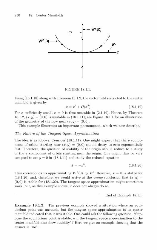
250 18. Center Manifolds
FIGURE 18.1.1.
Using (18.1.18) along with Theorem 18.1.2, the vector field restricted to the center
manifold is given by
x = x4+ O(x5
). (18.1.19)
For x sufficiently small, x = 0 is thus unstable in (2.1.19). Hence, by Theorem
18.1.2, (x, y) = (0, 0) is unstable in (18.1.11); see Figure 18.1.1 for an illustration
of the geometry of the flow near (x, y) = (0, 0).
This example illustrates an important phenomenon, which we now describe.
The Failure of the Tangent Space Approximation
The idea is as follows. Consider (18.1.11). One might expect that the y compo-
nents of orbits starting near (x, y) = (0, 0) should decay to zero exponentially
fast. Therefore, the question of stability of the origin should reduce to a study
of the x component of orbits starting near the origin. One might thus be very
tempted to set y = 0 in (18.1.11) and study the reduced equation
x = −x5. (18.1.20)
This corresponds to approximating W c(0) by Ec. However, x = 0 is stable for
(18.1.20) and, therefore, we would arrive at the wrong conclusion that (x, y) =
(0, 0) is stable for (18.1.20). The tangent space approximation might sometimes
work, but, as this example shows, it does not always do so.
End of Example 18.1.1
Example 18.1.2. The previous example showed a situation where an equi-
librium point was unstable, but the tangent space approximation to its center
manifold indicated that it was stable. One could ask the following question. “Sup-
pose the equilibrium point is stable, will the tangent space approximation to the
center manifold also show stability”? Here we give an example showing that the
answer is “no”.
18.2 Center Manifolds Depending on Parameters 251
Consider the vector field
x = −xy − x6,
y = −y + x2, (x, y) ∈ R2.
The origin is an equilibrium point, and the eigenvalues of the matrix associated
with the linearization are 0 and −1. The tangent space to the center manifold is
the x axis. Hence, the restriction of the vector field to the center manifold in thetangent space approximation is given by
x = −x6,
for which the origin is unstable.
The center manifold can be calculated, and it is given by the graph of the
following function
h(x) = x2+ O(4).
The vector field restricted to the center manifold is given by
x = −x3+ O(5),
which indicates that the origin is stable.
End of Example 18.1.2
18.2 Center Manifolds Depending on Parameters
Suppose (18.1.1) depends on a vector of parameters, say ε ∈ Rp. In this
case we write (2.1.2) in the form
x = Ax + f(x, y, ε),y = By + g(x, y, ε), (x, y, ε) ∈ R
c × Rs × R
p, (18.2.1)
where
f(0, 0, 0) = 0, Df(0, 0, 0) = 0,g(0, 0, 0) = 0, Dg(0, 0, 0) = 0,
and we have the same assumptions on A and B as in (18.1.1), with f and galso being Cr (r ≥ 2) functions in some neighborhood of (x, y, ε) = (0, 0, 0).An obvious question is why do we not allow the matrices A and B to dependon ε? This will be answered shortly.
The way in which we will handle parametrized systems is to include theparameter ε as a new dependent variable as follows
x = Ax + f(x, y, ε),ε = 0,
y = By + g(x, y, ε), (x, ε, y) ∈ Rc × R
p × Rs. (18.2.2)
252 18. Center Manifolds
At first glance it might appear that nothing is really gained from this action,but we will argue otherwise.
Let us suppose we are considering (18.2.2) afresh. It obviously has a fixedpoint at (x, ε, y) = (0, 0, 0). The matrix associated with the linearizationof (18.2.2) about this fixed point has c + p eigenvalues with zero real partand s eigenvalues with negative real part. Now let us apply center manifoldtheory. Modifying Definition 18.1.1, a center manifold will be representedas a graph over the x and ε variables, i.e., the graph of h(x, ε) for x and εsufficiently small. Theorem 18.1.2 still applies, with the vector field reducedto the center manifold given by
u = Au + f(u, h(u, ε), ε),ε = 0, (u, ε) ∈ R
c × Rp. (18.2.3)
Theorems 18.1.3 and 18.1.4 also follow (we will worry about any modifi-cations to computing the center manifold shortly). Thus, adding the pa-rameter as a new dependent variable merely acts to augment the matrix Ain (18.1.1) by adding p new center directions that have no dynamics, andthe theory goes through just the same. However, there is a new conceptwhich will be important when we study bifurcation theory ; namely, the cen-ter manifold exists for all ε in a sufficiently small neighborhood of ε = 0.We will learn in Chapters 20 and 21 that it is possible for solutions to becreated or destroyed by perturbing nonhyperbolic fixed points. Thus, sincethe invariant center manifold exists in a sufficiently small neighborhood inboth x and ε of (x, ε) = (0, 0), all bifurcating solutions will be contained inthe lower dimensional center manifold.
Let us now worry about computing the center manifold. From the exis-tence theorem for center manifolds, locally we have
W cloc(0) =
(x, ε, y) ∈ R
c × Rp × R
s | y = h(x, ε), |x| < δ,
|ε| < δ, h(0, 0) = 0, Dh(0, 0) = 0
(18.2.4)
for δ and δ sufficiently small. Using invariance of the graph of h(x, ε) underthe dynamics generated by (18.2.2) we have
y = Dxh(x, ε)x + Dεh(x, ε)ε = Bh(x, ε) + g (x, h(x, ε), ε) . (18.2.5)
However,
x = Ax + f (x, h(x, ε), ε) ,
ε = 0; (18.2.6)
hence substituting (18.2.6) into (18.2.5) results in the following quasilinearpartial differential equation that h(x, ε) must satisfy in order for its graphto be a center manifold.
N (h(x, ε)) = Dxh(x, ε) [Ax + f (x, h(x, ε), ε)]− Bh(x, ε)− g (x, h(x, ε), ε) = 0. (18.2.7)
18.2 Center Manifolds Depending on Parameters 253
Thus, we see that (18.2.7) is very similar to (18.1.10).Before considering a specific example we want to point out an important
fact. By considering ε as a new dependent variable, terms such as
xiεj , 1 ≤ i ≤ c, 1 ≤ j ≤ p,
oryiεj , 1 ≤ i ≤ s, 1 ≤ j ≤ p,
become nonlinear terms. In this case, returning to a question asked at thebeginning of this section, the parts of the matrices A and B dependingon ε are now viewed as nonlinear terms and are included in the f and gterms of (18.2.2), respectively. We remark that in applying center manifoldtheory to a given system, it must first be transformed into the standardform (either (18.1.1) or (18.2.2)).
Example 18.2.1 (The Lorenz Equations). Consider the Lorenz equations
x = σ(y − x),
y = ρx + x − y − xz, (x, y, z) ∈ R3, (18.2.8)
z = −βz + xy,
where σ and β are viewed as fixed positive constants and ρ is a parameter (note:
in the standard version of the Lorenz equations it is traditional to put ρ = ρ−1).
It should be clear that (x, y, z) = (0, 0, 0) is a fixed point of (18.2.9). Linearizing
(18.2.9) about this fixed point, we obtain the associated matrix−σ σ 0
1 −1 0
0 0 −β
. (18.2.9)
(Note: recall, ρx is a nonlinear term.)
Since (18.2.9) is in block form, the eigenvalues are particularly easy to compute
and are given by
0, −σ − 1, −β, (18.2.10)
with eigenvectors 1
1
0
,
σ−1
0
,
0
0
1
. (18.2.11)
Our goal is to determine the nature of the stability of (x, y, z) = (0, 0, 0) for ρnear zero. First, we must put (18.2.9) into the standard form (18.2.2). Using the
eigenbasis (18.2.11), we obtain the transformationxyz
=
1 σ 0
1 −1 0
0 0 1
uvw
(18.2.12)
with inverse uvw
=1
1 + σ
1 σ 0
1 −1 0
0 0 1 + σ
xyz
, (18.2.13)
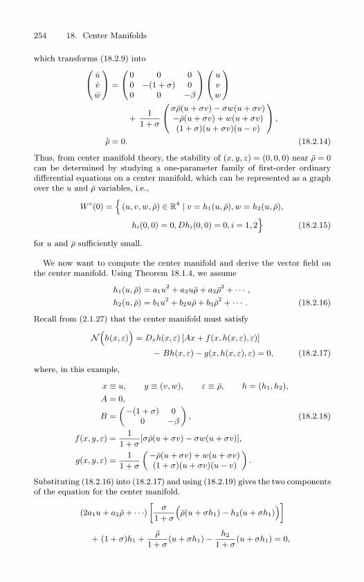
254 18. Center Manifolds
which transforms (18.2.9) into uvw
=
0 0 0
0 −(1 + σ) 0
0 0 −β
uvw
+
1
1 + σ
σρ(u + σv) − σw(u + σv)
−ρ(u + σv) + w(u + σv)
(1 + σ)(u + σv)(u − v)
,
˙ρ = 0. (18.2.14)
Thus, from center manifold theory, the stability of (x, y, z) = (0, 0, 0) near ρ = 0
can be determined by studying a one-parameter family of first-order ordinary
differential equations on a center manifold, which can be represented as a graph
over the u and ρ variables, i.e.,
W c(0) =
(u, v, w, ρ) ∈ R
4 | v = h1(u, ρ), w = h2(u, ρ),
hi(0, 0) = 0, Dhi(0, 0) = 0, i = 1, 2
(18.2.15)
for u and ρ sufficiently small.
We now want to compute the center manifold and derive the vector field on
the center manifold. Using Theorem 18.1.4, we assume
h1(u, ρ) = a1u2
+ a2uρ + a3ρ2
+ · · · ,
h2(u, ρ) = b1u2
+ b2uρ + b3ρ2
+ · · · . (18.2.16)
Recall from (2.1.27) that the center manifold must satisfy
N(h(x, ε)
)= Dxh(x, ε) [Ax + f(x, h(x, ε), ε)]
− Bh(x, ε) − g(x, h(x, ε), ε) = 0, (18.2.17)
where, in this example,
x ≡ u, y ≡ (v, w), ε ≡ ρ, h = (h1, h2),
A = 0,
B =
(−(1 + σ) 0
0 −β
), (18.2.18)
f(x, y, ε) =1
1 + σ[σρ(u + σv) − σw(u + σv)],
g(x, y, ε) =1
1 + σ
(−ρ(u + σv) + w(u + σv)
(1 + σ)(u + σv)(u − v)
).
Substituting (18.2.16) into (18.2.17) and using (18.2.19) gives the two components
of the equation for the center manifold.
(2a1u + a2ρ + · · ·)[
σ
1 + σ
(ρ(u + σh1) − h2(u + σh1)
)]+ (1 + σ)h1 +
ρ
1 + σ(u + σh1) − h2
1 + σ(u + σh1) = 0,
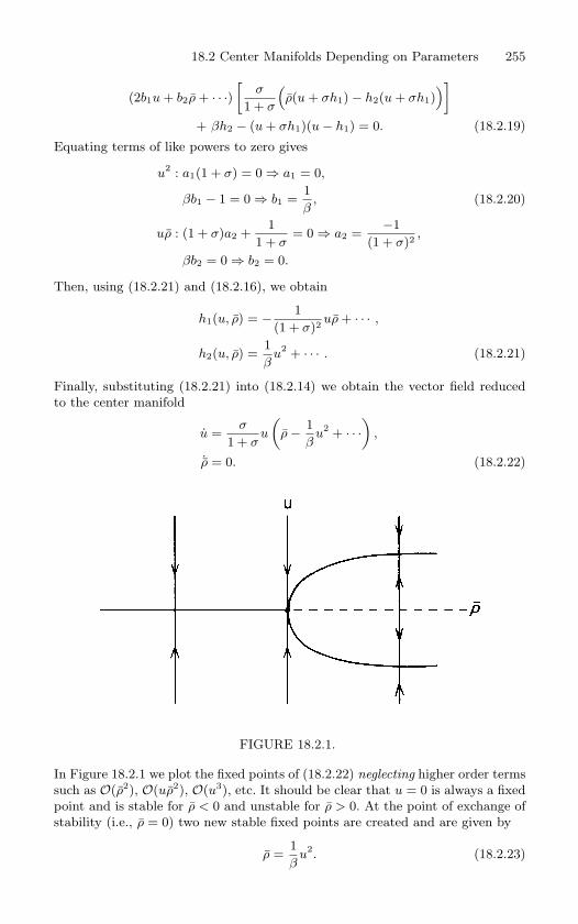
18.2 Center Manifolds Depending on Parameters 255
(2b1u + b2ρ + · · ·)[
σ
1 + σ
(ρ(u + σh1) − h2(u + σh1)
)]+ βh2 − (u + σh1)(u − h1) = 0. (18.2.19)
Equating terms of like powers to zero gives
u2: a1(1 + σ) = 0 ⇒ a1 = 0,
βb1 − 1 = 0 ⇒ b1 =1
β, (18.2.20)
uρ : (1 + σ)a2 +1
1 + σ= 0 ⇒ a2 =
−1
(1 + σ)2,
βb2 = 0 ⇒ b2 = 0.
Then, using (18.2.21) and (18.2.16), we obtain
h1(u, ρ) = − 1
(1 + σ)2uρ + · · · ,
h2(u, ρ) =1
βu2
+ · · · . (18.2.21)
Finally, substituting (18.2.21) into (18.2.14) we obtain the vector field reduced
to the center manifold
u =σ
1 + σu
(ρ − 1
βu2
+ · · ·)
,
˙ρ = 0. (18.2.22)
FIGURE 18.2.1.
In Figure 18.2.1 we plot the fixed points of (18.2.22) neglecting higher order terms
such as O(ρ2), O(uρ2), O(u3), etc. It should be clear that u = 0 is always a fixed
point and is stable for ρ < 0 and unstable for ρ > 0. At the point of exchange of
stability (i.e., ρ = 0) two new stable fixed points are created and are given by
ρ =1
βu2. (18.2.23)
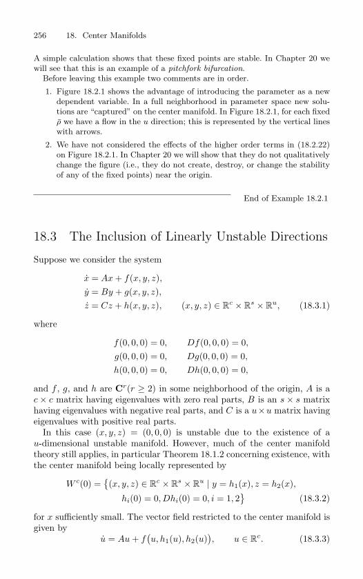
256 18. Center Manifolds
A simple calculation shows that these fixed points are stable. In Chapter 20 we
will see that this is an example of a pitchfork bifurcation.
Before leaving this example two comments are in order.
1. Figure 18.2.1 shows the advantage of introducing the parameter as a new
dependent variable. In a full neighborhood in parameter space new solu-
tions are “captured” on the center manifold. In Figure 18.2.1, for each fixed
ρ we have a flow in the u direction; this is represented by the vertical lines
with arrows.
2. We have not considered the effects of the higher order terms in (18.2.22)
on Figure 18.2.1. In Chapter 20 we will show that they do not qualitatively
change the figure (i.e., they do not create, destroy, or change the stability
of any of the fixed points) near the origin.
End of Example 18.2.1
18.3 The Inclusion of Linearly Unstable Directions
Suppose we consider the system
x = Ax + f(x, y, z),y = By + g(x, y, z),z = Cz + h(x, y, z), (x, y, z) ∈ R
c × Rs × R
u, (18.3.1)
where
f(0, 0, 0) = 0, Df(0, 0, 0) = 0,g(0, 0, 0) = 0, Dg(0, 0, 0) = 0,h(0, 0, 0) = 0, Dh(0, 0, 0) = 0,
and f , g, and h are Cr(r ≥ 2) in some neighborhood of the origin, A is ac× c matrix having eigenvalues with zero real parts, B is an s× s matrixhaving eigenvalues with negative real parts, and C is a u×u matrix havingeigenvalues with positive real parts.
In this case (x, y, z) = (0, 0, 0) is unstable due to the existence of au-dimensional unstable manifold. However, much of the center manifoldtheory still applies, in particular Theorem 18.1.2 concerning existence, withthe center manifold being locally represented by
W c(0) =(x, y, z) ∈ R
c × Rs × R
u | y = h1(x), z = h2(x),
hi(0) = 0, Dhi(0) = 0, i = 1, 2
(18.3.2)
for x sufficiently small. The vector field restricted to the center manifold isgiven by
u = Au + f(u, h1(u), h2(u)
), u ∈ R
c. (18.3.3)
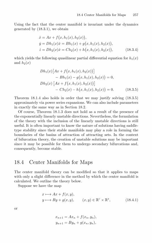
18.4 Center Manifolds for Maps 257
Using the fact that the center manifold is invariant under the dynamicsgenerated by (18.3.1), we obtain
x = Ax + f(x, h1(x), h2(x)
),
y = Dh1(x)x = Bh1(x) + g(x, h1(x), h2(x)
),
z = Dh2(x)x = Ch2(x) + h(x, h1(x), h2(x)
), (18.3.4)
which yields the following quasilinear partial differential equation for h1(x)and h2(x)
Dh1(x)[Ax + f
(x, h1(x), h2(x)
)]− Bh1(x)− g
(x, h1(x), h2(x)
)= 0,
Dh2(x)[Ax + f
(x, h1(x), h2(x)
)]− Ch2(x)− h
(x, h1(x), h2(x)
)= 0. (18.3.5)
Theorem 18.1.4 also holds in order that we may justify solving (18.3.5)approximately via power series expansions. We can also include parametersin exactly the same way as in Section 18.2.
Of course, Theorem 18.1.3 does not hold as a result of the presence ofthe exponentially linearly unstable directions. Nevertheless, the formulationof the theory with the inclusion of the linearly unstable directions is stilluseful. It is often important to know the nature of solutions having saddle-type stability since their stable manifolds may play a role in forming theboundaries of the basins of attraction of attracting sets. In the contextof bifurcation theory, the creation of unstable solutions may be importantsince it may be possible for them to undergo secondary bifurcations and,consequently, become stable.
18.4 Center Manifolds for Maps
The center manifold theory can be modified so that it applies to mapswith only a slight difference in the method by which the center manifold iscalculated. We outline the theory below.
Suppose we have the map
x −→ Ax + f(x, y),y −→ By + g(x, y), (x, y) ∈ R
c × Rs, (18.4.1)
or
xn+1 = Axn + f(xn, yn),yn+1 = Byn + g(xn, yn),
258 18. Center Manifolds
where
f(0, 0) = 0, Df(0, 0) = 0,g(0, 0) = 0, Dg(0, 0) = 0,
and f and g are Cr(r ≥ 2) in some neighborhood of the orgin, A is a c× cmatrix with eigenvalues of modulus one, and B is an s × s matrix witheigenvalues of modulus less than one.
Evidently (x, y) = (0, 0) is a fixed point of (18.4.1), and the linear approx-imation is not sufficient for determining its stability. We have the followingtheorems, which are completely analogous to Theorems 18.1.2, 18.1.3, and18.1.4.
Theorem 18.4.1 (Existence) There exists a Cr center manifold for
(18.4.1) which can be locally represented as a graph as follows
W c(0) = (x, y) ∈ Rc × R
s | y = h(x), |x| < δ, h(0) = 0, Dh(0) = 0(18.4.2)
for δ sufficiently small. Moreover, the dynamics of (18.4.1) restricted to
the center manifold is, for u sufficiently small, given by the c-dimensional
map
u −→ Au + f(u, h(u)
), u ∈ R
c. (18.4.3)
Proof: See Carr [1981].
The next theorem allows us to conclude that (x, y) = (0, 0) is stable orunstable based on whether or not u = 0 is stable or unstable in (18.4.3).
Theorem 18.4.2 (Stability) i) Suppose the zero solution of (18.4.3) is
stable (asymptotically stable) (unstable). Then the zero solution of (18.4.1)
is stable (asymptotically stable) (unstable). ii) Suppose that the zero solution
of (18.4.3) is stable. Let (xn, yn) be a solution of (18.4.1) with (x0, y0)sufficiently small. Then there is a solution un of (18.4.3) such that |xn −un| ≤ kβn and |yn − h(un)| ≤ kβn for all n where k and β are positive
constants with β < 1.
Proof: See Carr [1981].
Next we want to compute the center manifold so that we can derive(18.4.3). This is done in exactly the same way as for vector fields, i.e., byderiving a nonlinear functional equation that the graph of h(x) must satisfyin order for it to be invariant under the dynamics generated by (18.4.1). Inthis case we have
xn+1 = Axn + f(xn, h(xn)
),
yn+1 = h(xn+1) = Bh(xn) + g(xn, h(xn)
), (18.4.4)
18.4 Center Manifolds for Maps 259
or
N(h(x)
)= h
(Ax + f
(x, h(x))
)−Bh(x)− g
(x, h(x)
)= 0. (18.4.5)
(Note: the reader should compare (18.4.5) with (18.1.10).) The next theo-rem justifies the approximate solution of (18.4.5) via power series expan-sions.
Theorem 18.4.3 (Approximation) Let φ : Rc → R
s be a C1 map with
φ(0) = 0, φ′(0) = 0, and N(φ(x)
)= O(|x|q) as x → 0 for some q > 1.
Then
h(x) = φ(x) +O(|x|q) as x → 0.
Proof: See Carr [1981].
We now give an example.
Example 18.4.1. Consider the map uvw
→−1 0 0
0 − 12 0
0 0 12
uvw
+
vwu2
−uv
, (u, v, w) ∈ R3. (18.4.6)
It should be clear that (u, v, w) = (0, 0, 0) is a fixed point of (18.4.6), and the
eigenvalues associated with the map linearized about this fixed point are −1, − 12 ,
12 . Thus, the linear approximation does not suffice to determine the stability or
instability. We will apply center manifold theory to this problem.
The center manifold can locally be represented as follows
W c(0) =
(u, v, w) ∈ R
3 | v = h1(u), w = h2(u), hi(0) = 0,
Dhi(0) = 0, i = 1, 2
(18.4.7)
for u sufficiently small. Recall that the center manifold must satisfy the following
equation
N(h(x)
)= h
(Ax + f
(x, h(x)
))− Bh(x) − g
(x, h(x)
)= 0, (18.4.8)
where, in this example,
x = u, y ≡ (v, w), h = (h1, h2),
A = −1,
B =
(− 12 0
0 12
),
f(u, v, w) = vw,
g(u, v, w) =
(u2
−uv
). (18.4.9)
We assume a center manifold of the form
h(u) =
(h1(u)
h2(u)
)=
(a1u
2 + b1u3 + O(u4)
a2u2 + b2u
3 + O(u4)
). (18.4.10)
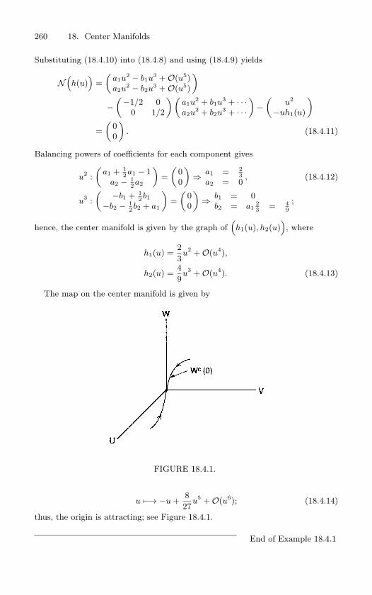
260 18. Center Manifolds
Substituting (18.4.10) into (18.4.8) and using (18.4.9) yields
N(h(u)
)=
(a1u
2 − b1u3 + O(u5)
a2u2 − b2u
3 + O(u5)
)−
(−1/2 0
0 1/2
)(a1u
2 + b1u3 + · · ·
a2u2 + b2u
3 + · · ·)
−(
u2
−uh1(u)
)=
(0
0
). (18.4.11)
Balancing powers of coefficients for each component gives
u2:
(a1 + 1
2a1 − 1
a2 − 12a2
)=
(0
0
)⇒ a1 = 2
3a2 = 0
, (18.4.12)
u3:
( −b1 + 12 b1
−b2 − 12 b2 + a1
)=
(0
0
)⇒ b1 = 0
b2 = a123 = 4
9;
hence, the center manifold is given by the graph of(h1(u), h2(u)
), where
h1(u) =2
3u2
+ O(u4),
h2(u) =4
9u3
+ O(u4). (18.4.13)
The map on the center manifold is given by
FIGURE 18.4.1.
u −→ −u +8
27u5
+ O(u6); (18.4.14)
thus, the origin is attracting; see Figure 18.4.1.
End of Example 18.4.1
18.4 Center Manifolds for Maps 261
Example 18.4.2. Consider the map(xy
)→
(0 1
− 12
32
)(xy
)+
(0
−y3
), (x, y) ∈ R
2. (18.4.15)
The origin is a fixed point of the map. Computing the eigenvalues of the map
linearized about the origin gives
λ1,2 = 1,1
2.
Therefore, there is a one-dimensional center manifold and a one-dimensional sta-
ble manifold with the orbit structure in a neighborhood of (0, 0) determined by
the orbit structure on the center manifold.
We wish to compute the center manifold, but first we must put the linear part
in block diagonal form as given in (18.4.1). The matrix associated with the linear
transformation has columns consisting of the eigenvectors of the linearized map
and is easily calculated. It is given by
T =
(1 2
1 1
)with T −1
=
(−1 2
1 −1
). (18.4.16)
Thus, letting (xy
)= T
(uv
),
our map becomes (uv
)→
(1 0
0 12
)(uv
)+
(−2(u + v)3
(u + v)3
). (18.4.17)
We seek a center manifold
W c(0) = (u, v) | v = h(u); h(0) = Dh(0) = 0 (18.4.18)
for u sufficiently small. The next step is to assume h(u) of the form
h(u) = au2+ bu3
+ O(u4) (18.4.19)
and substitute (18.4.19) into the center manifold equation
N(h(u)
)= h
(Au + f
(u, h(u)
))− Bh(u) − g
(u, h(u)
)= 0, (18.4.20)
where, in this example, we have
A = 1,
B =1
2,
f(u, v) = −2(u + v)3,
g(u, v) = (u + v)3, (18.4.21)
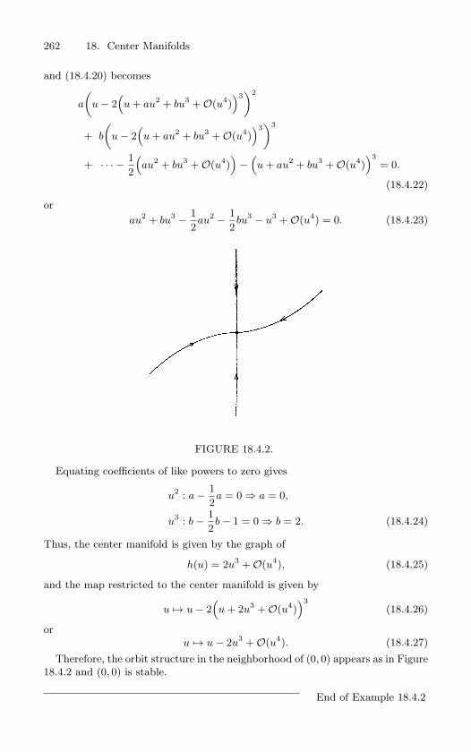
262 18. Center Manifolds
and (18.4.20) becomes
a
(u − 2
(u + au2
+ bu3+ O(u4
))3
)2
+ b
(u − 2
(u + au2
+ bu3+ O(u4
))3
)3
+ · · · − 1
2
(au2
+ bu3+ O(u4
))
−(u + au2
+ bu3+ O(u4
))3
= 0.
(18.4.22)
or
au2+ bu3 − 1
2au2 − 1
2bu3 − u3
+ O(u4) = 0. (18.4.23)
FIGURE 18.4.2.
Equating coefficients of like powers to zero gives
u2: a − 1
2a = 0 ⇒ a = 0,
u3: b − 1
2b − 1 = 0 ⇒ b = 2. (18.4.24)
Thus, the center manifold is given by the graph of
h(u) = 2u3+ O(u4
), (18.4.25)
and the map restricted to the center manifold is given by
u → u − 2(u + 2u3
+ O(u4))3
(18.4.26)
or
u → u − 2u3+ O(u4
). (18.4.27)
Therefore, the orbit structure in the neighborhood of (0, 0) appears as in Figure
18.4.2 and (0, 0) is stable.
End of Example 18.4.2
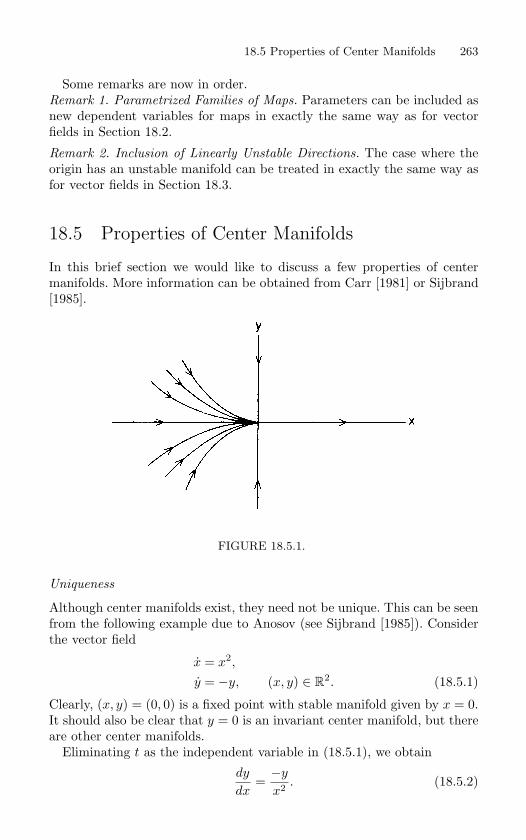
18.5 Properties of Center Manifolds 263
Some remarks are now in order.Remark 1. Parametrized Families of Maps. Parameters can be included asnew dependent variables for maps in exactly the same way as for vectorfields in Section 18.2.
Remark 2. Inclusion of Linearly Unstable Directions. The case where theorigin has an unstable manifold can be treated in exactly the same way asfor vector fields in Section 18.3.
18.5 Properties of Center Manifolds
In this brief section we would like to discuss a few properties of centermanifolds. More information can be obtained from Carr [1981] or Sijbrand[1985].
FIGURE 18.5.1.
Uniqueness
Although center manifolds exist, they need not be unique. This can be seenfrom the following example due to Anosov (see Sijbrand [1985]). Considerthe vector field
x = x2,
y = −y, (x, y) ∈ R2. (18.5.1)
Clearly, (x, y) = (0, 0) is a fixed point with stable manifold given by x = 0.It should also be clear that y = 0 is an invariant center manifold, but thereare other center manifolds.
Eliminating t as the independent variable in (18.5.1), we obtain
dy
dx=−y
x2 . (18.5.2)
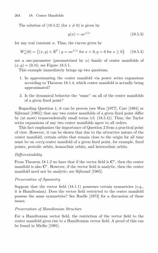
264 18. Center Manifolds
The solution of (18.5.2) (for x = 0) is given by
y(x) = αe1/x (18.5.3)
for any real constant α. Thus, the curves given by
W cα(0) =
(x, y) ∈ R
2 | y = αe1/x for x < 0, y = 0 for x ≥ 0
(18.5.4)
are a one-parameter (parametrized by α) family of center manifolds of(x, y) = (0, 0); see Figure 18.5.1.
This example immediately brings up two questions.
1. In approximating the center manifold via power series expansionsaccording to Theorem 18.1.4, which center manifold is actually beingapproximated?
2. Is the dynamical behavior the “same” on all of the center manifoldsof a given fixed point?
Regarding Question 1, it can be proven (see Wan [1977], Carr [1981] orSijbrand [1985]) that any two center manifolds of a given fixed point differby (at most) transcendentally small terms (cf. (18.5.4)). Thus, the Taylorseries expansions of any two center manifolds agree to all orders.
This fact emphasizes the importance of Question 2 from a practical pointof view. However, it can be shown that due to the attractive nature of thecenter manifold, certain orbits that remain close to the origin for all timemust be on every center manifold of a given fixed point, for example, fixedpoints, periodic orbits, homoclinic orbits, and heteroclinic orbits.
Differentiability
From Theorem 18.1.2 we have that if the vector field is Cr, then the centermanifold is also Cr. However, if the vector field is analytic, then the centermanifold need not be analytic; see Sijbrand [1985].
Preservation of Symmetry
Suppose that the vector field (18.1.1) possesses certain symmetries (e.g.,it is Hamiltonian). Does the vector field restricted to the center manifoldpossess the same symmetries? See Ruelle [1973] for a discussion of theseissues.
Preservation of Hamiltonian Structure
For a Hamiltonian vector field, the restriction of the vector field to thecenter manifold gives rise to a Hamiltonian vector field. A proof of this canbe found in Mielke [1991].
18.6 Final Remarks on Center Manifolds 265
18.6 Final Remarks on Center Manifolds
A Coordinate Independent Center Manifold Reduction. We devel-oped center manifold theory by assuming that the linear part of thevector field was in block diagonal form, see, e.g., (18.1.1). However,Leen [1993] has developed a coordinate independent approach to thecenter manifold reduction.
Center Manifolds for Stochastic Dynamical Systems. A center man-ifold theory for stochastic dynamical systems has been developed byBoxler [1989], [1991].
18.7 Exercises1. Consider the Cr (r ≥ 1) map
x → f(x), x ∈ Rn
. (18.7.1)
Suppose that the map has a fixed point at x = x0, i.e.,
x0 = f(x0).
Next consider the vector fieldx = f(x) − x. (18.7.2)
Clearly (18.7.2) has a fixed point, and x = x0. What can you determine about theorbit structure near the fixed point of the map (18.7.1) based on knowledge of theorbit structure near the fixed point x = x0 of the vector field (18.7.2)?
2. Consider the Cr mapf : R
1 → R1
and denote the Taylor expansion of f by
f(x) = a0 + a1x + · · · + ar−1xr−1 + O(|x|r).
Suppose f is identically zero. Then show that ai = 0, i = 0, . . . , r − 1. Does the sameresult hold for the Cr map
f : Rn → R
n, n > 1?
3. Study the dynamics near the origin for each of the following vector fields. Draw phaseportraits. Compute the center manifolds and describe the dynamics on the centermanifold. Discuss the stability or instability of the origin.
a) θ = −θ + v2,
v = − sin θ,(θ, v) ∈ S
1 × R1.
b) x =12
x + y + x2y,
y = x + 2y + y2,
(x, y) ∈ R2.
c)x = x − 2y,
y = 3x − y − x2,
(x, y) ∈ R2.
d)x = 2x + 2y,
y = x + y + x4,
(x, y) ∈ R2.
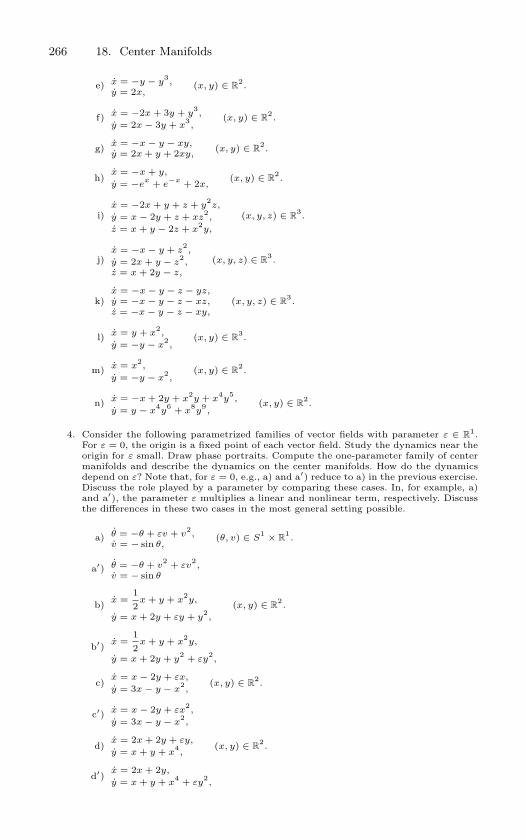
266 18. Center Manifolds
e) x = −y − y3,
y = 2x,(x, y) ∈ R
2.
f) x = −2x + 3y + y3,
y = 2x − 3y + x3,
(x, y) ∈ R2.
g) x = −x − y − xy,y = 2x + y + 2xy,
(x, y) ∈ R2.
h)x = −x + y,
y = −ex + e
−x + 2x,(x, y) ∈ R
2.
i)x = −2x + y + z + y
2z,
y = x − 2y + z + xz2,
z = x + y − 2z + x2y,
(x, y, z) ∈ R3.
j)x = −x − y + z
2,
y = 2x + y − z2,
z = x + 2y − z,
(x, y, z) ∈ R3.
k)x = −x − y − z − yz,y = −x − y − z − xz,z = −x − y − z − xy,
(x, y, z) ∈ R3.
l) x = y + x2,
y = −y − x2,
(x, y) ∈ R3.
m) x = x2,
y = −y − x2,
(x, y) ∈ R2.
n) x = −x + 2y + x2y + x
4y5,
y = y − x4y6 + x
8y9,
(x, y) ∈ R2.
4. Consider the following parametrized families of vector fields with parameter ε ∈ R1.
For ε = 0, the origin is a fixed point of each vector field. Study the dynamics near theorigin for ε small. Draw phase portraits. Compute the one-parameter family of centermanifolds and describe the dynamics on the center manifolds. How do the dynamicsdepend on ε? Note that, for ε = 0, e.g., a) and a′) reduce to a) in the previous exercise.Discuss the role played by a parameter by comparing these cases. In, for example, a)and a′), the parameter ε multiplies a linear and nonlinear term, respectively. Discussthe differences in these two cases in the most general setting possible.
a) θ = −θ + εv + v2,
v = − sin θ,(θ, v) ∈ S
1 × R1.
a′) θ = −θ + v2 + εv
2,
v = − sin θ
b) x =12
x + y + x2y,
y = x + 2y + εy + y2,
(x, y) ∈ R2.
b′) x =12
x + y + x2y,
y = x + 2y + y2 + εy
2,
c)x = x − 2y + εx,
y = 3x − y − x2,
(x, y) ∈ R2.
c′) x = x − 2y + εx2,
y = 3x − y − x2,
d)x = 2x + 2y + εy,
y = x + y + x4,
(x, y) ∈ R2.
d′)x = 2x + 2y,
y = x + y + x4 + εy
2,
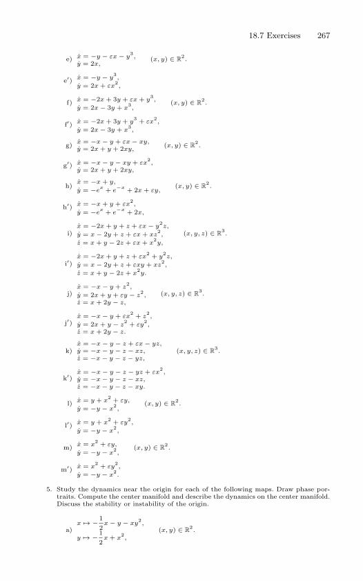
18.7 Exercises 267
e) x = −y − εx − y3,
y = 2x,(x, y) ∈ R
2.
e′) x = −y − y3,
y = 2x + εx2,
f) x = −2x + 3y + εx + y3,
y = 2x − 3y + x3,
(x, y) ∈ R2.
f′) x = −2x + 3y + y3 + εx
2,
y = 2x − 3y + x3,
g) x = −x − y + εx − xy,y = 2x + y + 2xy,
(x, y) ∈ R2.
g′) x = −x − y − xy + εx2,
y = 2x + y + 2xy,
h)x = −x + y,
y = −ex + e
−x + 2x + εy,(x, y) ∈ R
2.
h′) x = −x + y + εx2,
y = −ex + e
−x + 2x,
i)x = −2x + y + z + εx − y
2z,
y = x − 2y + z + εx + xz2,
z = x + y − 2z + εx + x2y,
(x, y, z) ∈ R3.
i′)x = −2x + y + z + εx
2 + y2z,
y = x − 2y + z + εxy + xz2,
z = x + y − 2z + x2y.
j)x = −x − y + z
2,
y = 2x + y + εy − z2,
z = x + 2y − z,
(x, y, z) ∈ R3.
j′)x = −x − y + εx
2 + z2,
y = 2x + y − z2 + εy
2,
z = x + 2y − z.
k)x = −x − y − z + εx − yz,y = −x − y − z − xz,z = −x − y − z − yz,
(x, y, z) ∈ R3.
k′)x = −x − y − z − yz + εx
2,
y = −x − y − z − xz,z = −x − y − z − xy.
l) x = y + x2 + εy,
y = −y − x2,
(x, y) ∈ R2.
l′) x = y + x2 + εy
2,
y = −y − x2,
m) x = x2 + εy,
y = −y − x2,
(x, y) ∈ R2.
m′) x = x2 + εy
2,
y = −y − x2.
5. Study the dynamics near the origin for each of the following maps. Draw phase por-traits. Compute the center manifold and describe the dynamics on the center manifold.Discuss the stability or instability of the origin.
a)x → − 1
2x − y − xy
2,
y → − 12
x + x2,
(x, y) ∈ R2.
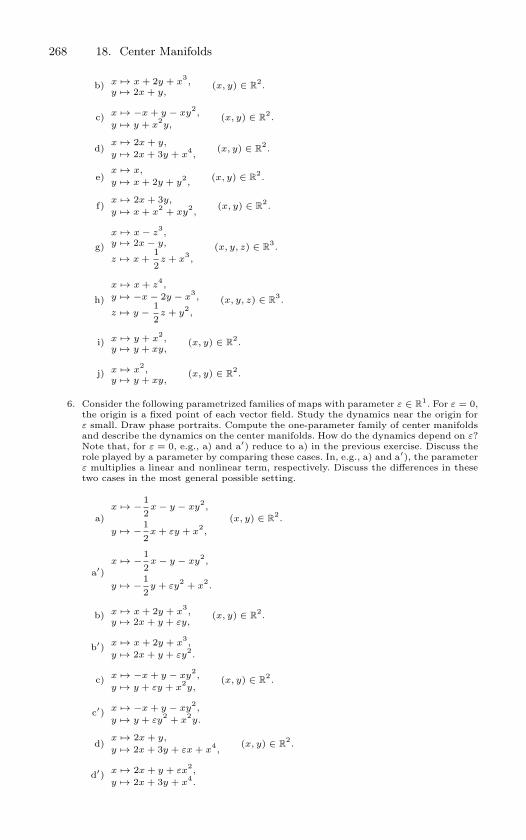
268 18. Center Manifolds
b) x → x + 2y + x3,
y → 2x + y,(x, y) ∈ R
2.
c) x → −x + y − xy2,
y → y + x2y,
(x, y) ∈ R2.
d)x → 2x + y,
y → 2x + 3y + x4,
(x, y) ∈ R2.
e)x → x,
y → x + 2y + y2,
(x, y) ∈ R2.
f)x → 2x + 3y,
y → x + x2 + xy
2,
(x, y) ∈ R2.
g)
x → x − z3,
y → 2x − y,
z → x +12
z + x3,
(x, y, z) ∈ R3.
h)
x → x + z4,
y → −x − 2y − x3,
z → y − 12
z + y2,
(x, y, z) ∈ R3.
i) x → y + x2,
y → y + xy,(x, y) ∈ R
2.
j) x → x2,
y → y + xy,(x, y) ∈ R
2.
6. Consider the following parametrized families of maps with parameter ε ∈ R1. For ε = 0,
the origin is a fixed point of each vector field. Study the dynamics near the origin forε small. Draw phase portraits. Compute the one-parameter family of center manifoldsand describe the dynamics on the center manifolds. How do the dynamics depend on ε?Note that, for ε = 0, e.g., a) and a′) reduce to a) in the previous exercise. Discuss therole played by a parameter by comparing these cases. In, e.g., a) and a′), the parameterε multiplies a linear and nonlinear term, respectively. Discuss the differences in thesetwo cases in the most general possible setting.
a)x → − 1
2x − y − xy
2,
y → − 12
x + εy + x2,
(x, y) ∈ R2.
a′)x → − 1
2x − y − xy
2,
y → − 12
y + εy2 + x
2.
b) x → x + 2y + x3,
y → 2x + y + εy,(x, y) ∈ R
2.
b′) x → x + 2y + x3,
y → 2x + y + εy2.
c) x → −x + y − xy2,
y → y + εy + x2y,
(x, y) ∈ R2.
c′) x → −x + y − xy2,
y → y + εy2 + x
2y.
d)x → 2x + y,
y → 2x + 3y + εx + x4,
(x, y) ∈ R2.
d′) x → 2x + y + εx2,
y → 2x + 3y + x4.
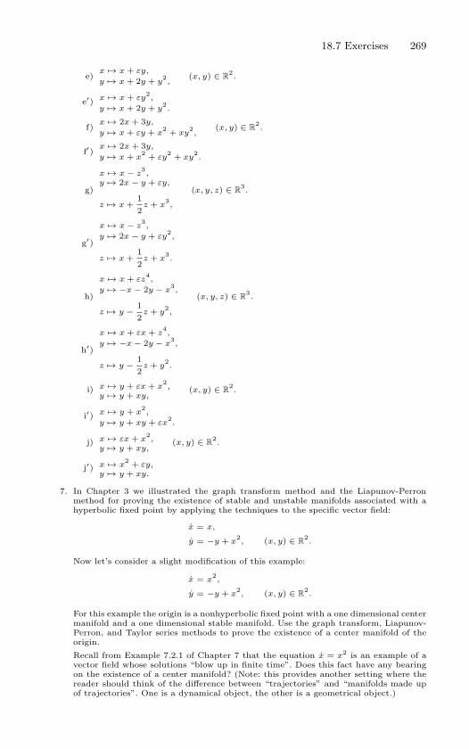
18.7 Exercises 269
e)x → x + εy,
y → x + 2y + y2,
(x, y) ∈ R2.
e′) x → x + εy2,
y → x + 2y + y2.
f)x → 2x + 3y,
y → x + εy + x2 + xy
2,
(x, y) ∈ R2.
f′)x → 2x + 3y,
y → x + x2 + εy
2 + xy2.
g)
x → x − z3,
y → 2x − y + εy,
z → x +12
z + x3,
(x, y, z) ∈ R3.
g′)
x → x − z3,
y → 2x − y + εy2,
z → x +12
z + x3.
h)
x → x + εz4,
y → −x − 2y − x3,
z → y − 12
z + y2,
(x, y, z) ∈ R3.
h′)
x → x + εx + z4,
y → −x − 2y − x3,
z → y − 12
z + y2.
i) x → y + εx + x2,
y → y + xy,(x, y) ∈ R
2.
i′) x → y + x2,
y → y + xy + εx2.
j) x → εx + x2,
y → y + xy,(x, y) ∈ R
2.
j′) x → x2 + εy,
y → y + xy.
7. In Chapter 3 we illustrated the graph transform method and the Liapunov-Perronmethod for proving the existence of stable and unstable manifolds associated with ahyperbolic fixed point by applying the techniques to the specific vector field:
x = x,
y = −y + x2, (x, y) ∈ R
2.
Now let’s consider a slight modification of this example:
x = x2,
y = −y + x2, (x, y) ∈ R
2.
For this example the origin is a nonhyperbolic fixed point with a one dimensional centermanifold and a one dimensional stable manifold. Use the graph transform, Liapunov-Perron, and Taylor series methods to prove the existence of a center manifold of theorigin.
Recall from Example 7.2.1 of Chapter 7 that the equation x = x2 is an example of avector field whose solutions “blow up in finite time”. Does this fact have any bearingon the existence of a center manifold? (Note: this provides another setting where thereader should think of the difference between “trajectories” and “manifolds made upof trajectories”. One is a dynamical object, the other is a geometrical object.)
19
Normal Forms
The method of normal forms provides a way of finding a coordinate systemin which the dynamical system takes the “simplest” form, where the term“simplest” will be defined as we go along. As we develop the method, threeimportant characteristics should become apparent.
1. The method is local in the sense that the coordinate transformationsare generated in a neighborhood of a known solution. For our pur-poses, the known solution will be a fixed point. However, when wedevelop the theory for maps, the results will have immediate applica-tions to periodic orbits of vector fields by considering the associatedPoincare map (cf. Chapter 10).
2. In general, the coordinate transformations will be nonlinear functionsof the dependent variables. However, the important point is that thesecoordinate transformations are found by solving a sequence of linear
problems.
3. The structure of the normal form is determined entirely by the natureof the linear part of the vector field.
We now begin the development of the method.
19.1 Normal Forms for Vector Fields
Consider the vector field
w = G(w), w ∈ Rn, (19.1.1)
where G is Cr, with r to be specified as we go along (note: in practice wewill need r ≥ 4). Suppose (19.1.1) has a fixed point at w = w0.
19.1a Preliminary Preparation of the EquationsWe first want to perform a few simple (linear) coordinate transformationsthat will put (19.1.1) into a form which is easier to work with.
19.1 Normal Forms for Vector Fields 271
1. First we transform the fixed point to the origin by the translation
v = w − w0, v ∈ Rn,
under which (19.1.1) becomes
v = G(v + w0) ≡ H(v). (19.1.2)
2. We next “split off” the linear part of the vector field and write (19.1.2)as follows
v = DH(0)v + H(v), (19.1.3)
where H(v) ≡ H(v) − DH(0)v. It should be clear that H(v) =O(|v|2).
3. Finally, let T be the matrix that transforms the matrix DH(0) into(real) Jordan canonical form. Then, under the transformation
v = Tx, (19.1.4)
(19.1.3) becomes
x = T−1DH(0)Tx + T−1H(Tx). (19.1.5)
Denoting the (real) Jordan canonical form of DH(0) by J , we have
J ≡ T−1DH(0)T, (19.1.6)
and we defineF (x) ≡ T−1H(Tx)
so that (19.1.4) is alternately written as
x = Jx + F (x), x ∈ Rn. (19.1.7)
We remark that the transformation (19.1.4) has simplified the lin-ear part of (19.1.3) as much as possible. We now begin the task ofsimplifying the nonlinear part, F (x).
First, we Taylor expand F (x) so that (19.1.7) becomes
x = Jx + F2(x) + F3(x) + · · ·+ Fr−1(x) +O(|x|r), (19.1.8)
where Fi(x) represent the order i terms in the Taylor expansion of F (x).
272 19. Normal Forms
19.1b Simplification of the Second Order TermsWe next introduce the coordinate transformation
x = y + h2(y), (19.1.9)
where h2(y) is second order in y. Substituting (19.1.9) into (19.1.8) gives
x =(id +Dh2(y)
)y = Jy + Jh2(y) + F2
(y + h2(y)
)+F3
(y + h2(y)
)+ · · ·+ Fr−1
(y + h2(y)
)+O(|y|r),(19.1.10)
where “id” denotes the n× n identity matrix. Note that each term
Fk
(y + h2(y)
), 2 ≤ k ≤ r − 1, (19.1.11)
can be written as
Fk(y) +O(|y|k+1) + · · ·+O(|y|2k), (19.1.12)
so that (19.1.10) becomes(id +Dh2(y)
)y = Jy + Jh2(y) + F2(y) + F3(y)
+ · · ·+ Fr−1(y) +O(|y|r), (19.1.13)
where the change of notation for the O(|y|k) terms, to Fk(y), serves todenote that they have been modified as a result of the coordinate transfor-mation.
Now, for y sufficiently small,(id +Dh2(y)
)−1 (19.1.14)
exists and can be represented in a series expansion as follows (see Exercise3) (
id +Dh2(y))−1 = id−Dh2(y) +O(|y|2). (19.1.15)
Substituting (19.1.15) into (19.1.13) gives
y = Jy + Jh2(y)−Dh2(y)Jy + F2(y) + F3(y)+ · · ·+ Fr−1(y) +O(|y|r). (19.1.16)
Up to this point h2(y) has been completely arbitrary. However, now wewill choose a specific form for h2(y) so as to simplify the O(|y|2) terms asmuch as possible. Ideally, this would mean choosing h2(y) such that
Dh2(y)Jy − Jh2(y) = F2(y), (19.1.17)
which would eliminate F2(y) from (19.1.16). Equation (19.1.17) can beviewed as an equation for the unknown h2(y). We want to motivate thefact that, when viewed in the correct way, it is in fact a linear equationacting on a linear vector space. This will be accomplished by 1) definingthe appropriate linear vector space; 2) defining the linear operator on thevector space; and 3) describing the equation to be solved in this linearvector space (which will turn out to be (19.1.17)). We begin with Step 1.
19.1 Normal Forms for Vector Fields 273
Step 1. The Space of Vector-Valued Homogeneous Polynomials of Degree
k, Hk
Let s1, · · · , sn denote a basis of Rn, and let y = (y1, · · · , yn) be coordi-
nates with respect to this basis. Now consider those basis elements withcoefficients consisting of homogeneous polynomials of degree k, i.e.,
(ym11 ym2
2 · · · ymnn )si,
n∑j=1
mj = k, (19.1.18)
where mj ≥ 0 are integers. We refer to these objects as vector-valued homo-
geneous polynomials of degree k. The set of all vector-valued homogeneouspolynomials of degree k forms a linear vector space, which we denote byHk. An obvious basis for Hk consists of elements formed by considering allpossible homogeneous polynomials of degree k that multiply each si. Thereader should verify these statements. Let us consider a specific example.
Example 19.1.1. We consider the standard basis(1
0
),
(0
1
)(19.1.19)
on R2 and denote the coordinates with respect to this basis by x and y, respec-
tively. Then we have
H2 = Span
(x2
0
),
(xy0
),
(y2
0
),
(0
x2
),
(0
xy
),
(0
y2
). (19.1.20)
End of Example 19.1.1
Step 2. The Linear Map on Hk
Now let us reconsider equation (19.1.17). It should be clear that h2(y) canbe viewed as an element of H2. The reader should easily be able to verifythat the map
h2(y) −→ Dh2(y)Jy − Jh2(y) (19.1.21)
is a linear map of H2 into H2. Indeed, for any element hk(y) ∈ Hk, itsimilarly follows that
hk(y) −→ Dhk(y)Jy − Jhk(y) (19.1.22)
is a linear map of Hk into Hk.Let us mention some terminology associated with Eq. (19.1.17) that has
become traditional. Due to its presence in Lie algebra theory (see, e.g.,Olver [1986]) this map is often denoted as
L(k)J
(hk(y)
)≡ −
(Dhk(y)Jy − Jhk(y)
)(19.1.23)
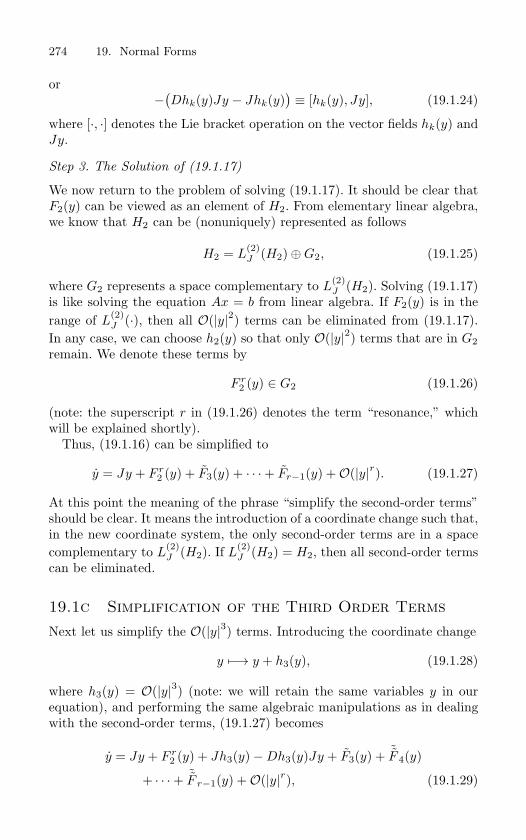
274 19. Normal Forms
or−(Dhk(y)Jy − Jhk(y)
)≡ [hk(y), Jy], (19.1.24)
where [·, ·] denotes the Lie bracket operation on the vector fields hk(y) andJy.
Step 3. The Solution of (19.1.17)
We now return to the problem of solving (19.1.17). It should be clear thatF2(y) can be viewed as an element of H2. From elementary linear algebra,we know that H2 can be (nonuniquely) represented as follows
H2 = L(2)J (H2)⊕G2, (19.1.25)
where G2 represents a space complementary to L(2)J (H2). Solving (19.1.17)
is like solving the equation Ax = b from linear algebra. If F2(y) is in therange of L
(2)J (·), then all O(|y|2) terms can be eliminated from (19.1.17).
In any case, we can choose h2(y) so that only O(|y|2) terms that are in G2remain. We denote these terms by
F r2 (y) ∈ G2 (19.1.26)
(note: the superscript r in (19.1.26) denotes the term “resonance,” whichwill be explained shortly).
Thus, (19.1.16) can be simplified to
y = Jy + F r2 (y) + F3(y) + · · ·+ Fr−1(y) +O(|y|r). (19.1.27)
At this point the meaning of the phrase “simplify the second-order terms”should be clear. It means the introduction of a coordinate change such that,in the new coordinate system, the only second-order terms are in a spacecomplementary to L
(2)J (H2). If L
(2)J (H2) = H2, then all second-order terms
can be eliminated.
19.1c Simplification of the Third Order TermsNext let us simplify the O(|y|3) terms. Introducing the coordinate change
y −→ y + h3(y), (19.1.28)
where h3(y) = O(|y|3) (note: we will retain the same variables y in ourequation), and performing the same algebraic manipulations as in dealingwith the second-order terms, (19.1.27) becomes
y = Jy + F r2 (y) + Jh3(y)−Dh3(y)Jy + F3(y) + ˜F 4(y)
+ · · ·+ ˜F r−1(y) +O(|y|r), (19.1.29)
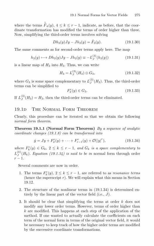
19.1 Normal Forms for Vector Fields 275
where the terms ˜F k(y), 4 ≤ k ≤ r − 1, indicate, as before, that the coor-dinate transformation has modified the terms of order higher than three.Now, simplifying the third-order terms involves solving
Dh3(y)Jy − Jh3(y) = F3(y). (19.1.30)
The same comments as for second-order terms apply here. The map
h3(y) −→ Dh3(y)Jy − Jh3(y) ≡ −L(3)J (h3(y)) (19.1.31)
is a linear map of H3 into H3. Thus, we can write
H3 = L(3)J (H3)⊕G3, (19.1.32)
where G3 is some space complementary to L(3)J (H3). Thus, the third-order
terms can be simplified toF r
3 (y) ∈ G3. (19.1.33)
If L(3)J (H3) = H3, then the third-order terms can be eliminated.
19.1d The Normal Form TheoremClearly, this procedure can be iterated so that we obtain the followingnormal form theorem.
Theorem 19.1.1 (Normal Form Theorem) By a sequence of analytic
coordinate changes (19.1.8) can be transformed into
y = Jy + F r2 (y) + · · ·+ F r
r−1(y) +O(|y|r), (19.1.34)
where F rk (y) ∈ Gk, 2 ≤ k ≤ r − 1, and Gk is a space complementary to
L(k)J (Hk). Equation (19.1.34) is said to be in normal form through order
r − 1.
Several comments are now in order.
1. The terms F rk (y), 2 ≤ k ≤ r − 1, are referred to as resonance terms
(hence the superscript r). We will explain what this means in Section19.12.
2. The structure of the nonlinear terms in (19.1.34) is determined en-tirely by the linear part of the vector field (i.e., J).
3. It should be clear that simplifying the terms at order k does notmodify any lower order terms. However, terms of order higher thank are modified. This happens at each step of the application of themethod. If one wanted to actually calculate the coefficients on eachterm of the normal form in terms of the original vector field, it wouldbe necessary to keep track of how the higher order terms are modifiedby the successive coordinate transformations.
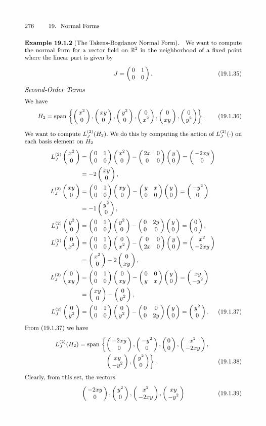
276 19. Normal Forms
Example 19.1.2 (The Takens-Bogdanov Normal Form). We want to compute
the normal form for a vector field on R2 in the neighborhood of a fixed point
where the linear part is given by
J =
(0 1
0 0
). (19.1.35)
Second-Order Terms
We have
H2 = span
(x2
0
),
(xy0
),
(y2
0
),
(0
x2
),
(0
xy
),
(0
y2
). (19.1.36)
We want to compute L(2)J (H2). We do this by computing the action of L
(2)J (·) on
each basis element on H2
L(2)J
(x2
0
)=
(0 1
0 0
)(x2
0
)−
(2x 0
0 0
)(y0
)=
(−2xy0
)= −2
(xy0
),
L(2)J
(xy0
)=
(0 1
0 0
)(xy0
)−
(y x0 0
)(y0
)=
(−y2
0
)= −1
(y2
0
),
L(2)J
(y2
0
)=
(0 1
0 0
)(y2
0
)−
(0 2y0 0
)(y0
)=
(0
0
),
L(2)J
(0
x2
)=
(0 1
0 0
)(0
x2
)−
(0 0
2x 0
)(y0
)=
(x2
−2xy
)=
(x2
0
)− 2
(0
xy
),
L(2)J
(0
xy
)=
(0 1
0 0
)(0
xy
)−
(0 0
y x
)(y0
)=
(xy
−y2
)=
(xy0
)−
(0
y2
),
L(2)J
(0
y2
)=
(0 1
0 0
)(0
y2
)−
(0 0
0 2y
)(y0
)=
(y2
0
). (19.1.37)
From (19.1.37) we have
L(2)J (H2) = span
(−2xy0
),
(−y2
0
),
(0
0
),
(x2
−2xy
),(
xy−y2
),
(y2
0
). (19.1.38)
Clearly, from this set, the vectors(−2xy0
),
(y2
0
),
(x2
−2xy
),
(xy
−y2
)(19.1.39)
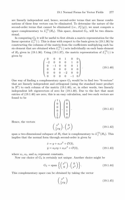
19.1 Normal Forms for Vector Fields 277
are linearly independent and, hence, second-order terms that are linear combi-
nations of these four vectors can be eliminated. To determine the nature of the
second-order terms that cannot be eliminated (i.e., F r2 (y)), we must compute a
space complementary to L(2)J (H2). This space, denoted G2, will be two dimen-
sional.
In computing G2 it will be useful to first obtain a matrix representation for the
linear operator L(2)J (·). This is done with respect to the basis given in (19.1.36) by
constructing the columns of the matrix from the coefficients multiplying each ba-
sis element that are obtained when L(2)J (·) acts individually on each basis element
of H2 given in (19.1.36). Using (19.1.37), the matrix representation of L(2)J (·) is
given by 0 0 0 1 0 0
−2 0 0 0 1 0
0 −1 0 0 0 1
0 0 0 0 0 0
0 0 0 −2 0 0
0 0 0 0 −1 0
. (19.1.40)
One way of finding a complementary space G2 would be to find two “6-vectors”
that are linearly independent and orthogonal (using the standard inner product
in R6) to each column of the matrix (19.1.40), or, in other words, two linearly
independent left eigenvectors of zero for (19.1.40). Due to the fact that most
entries of (19.1.40) are zero, this is an easy calculation, and two such vectors are
found to be 1
0
0
0120
,
0
0
0
1
0
0
. (19.1.41)
Hence, the vectors (x2
12xy
),
(0
x2
)(19.1.42)
span a two-dimensional subspace of H2 that is complementary to L(2)J (H2). This
implies that the normal form through second-order is given by
x = y + a1x2
+ O(3),
y = a2xy + a3x2
+ O(3), (19.1.43)
where a1, a2, and a3 represent constants.
Now our choice of G2 is certainly not unique. Another choice might be
G2 = span
(x2
0
),
(0
x2
). (19.1.44)
This complementary space can be obtained by taking the vector(x2
12xy
)(19.1.45)
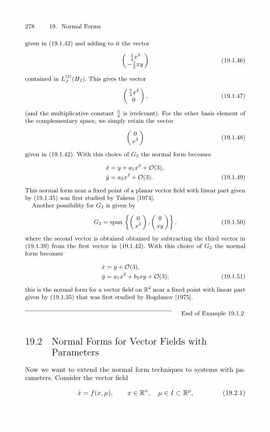
278 19. Normal Forms
given in (19.1.42) and adding to it the vector( 14x2
− 12xy
)(19.1.46)
contained in L(2)J (H2). This gives the vector( 5
4x2
0
), (19.1.47)
(and the multiplicative constant 54 is irrelevant). For the other basis element of
the complementary space, we simply retain the vector(0
x2
)(19.1.48)
given in (19.1.42). With this choice of G2 the normal form becomes
x = y + a1x2
+ O(3),
y = a2x2
+ O(3). (19.1.49)
This normal form near a fixed point of a planar vector field with linear part given
by (19.1.35) was first studied by Takens [1974].
Another possibility for G2 is given by
G2 = span
(0
x2
),
(0
xy
), (19.1.50)
where the second vector is obtained obtained by subtracting the third vector in
(19.1.39) from the first vector in (19.1.42). With this choice of G2 the normal
form becomes
x = y + O(3),
y = a1x2
+ b2xy + O(3); (19.1.51)
this is the normal form for a vector field on R2 near a fixed point with linear part
given by (19.1.35) that was first studied by Bogdanov [1975].
End of Example 19.1.2
19.2 Normal Forms for Vector Fields withParameters
Now we want to extend the normal form techniques to systems with pa-rameters. Consider the vector field
x = f(x, µ), x ∈ Rn, µ ∈ I ⊂ R
p, (19.2.1)
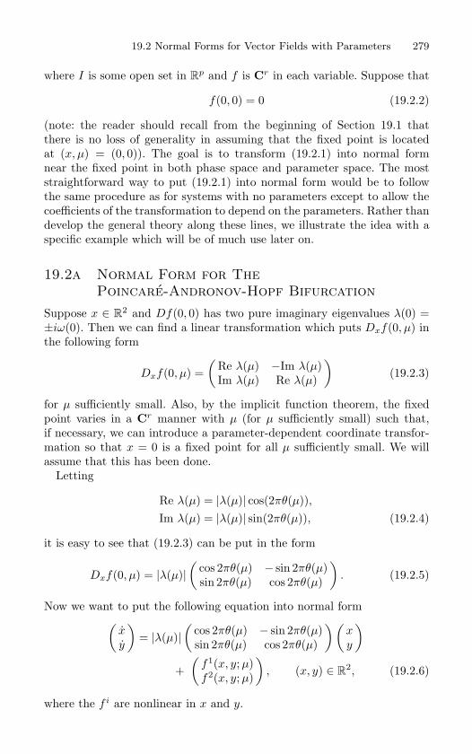
19.2 Normal Forms for Vector Fields with Parameters 279
where I is some open set in Rp and f is Cr in each variable. Suppose that
f(0, 0) = 0 (19.2.2)
(note: the reader should recall from the beginning of Section 19.1 thatthere is no loss of generality in assuming that the fixed point is locatedat (x, µ) = (0, 0)). The goal is to transform (19.2.1) into normal formnear the fixed point in both phase space and parameter space. The moststraightforward way to put (19.2.1) into normal form would be to followthe same procedure as for systems with no parameters except to allow thecoefficients of the transformation to depend on the parameters. Rather thandevelop the general theory along these lines, we illustrate the idea with aspecific example which will be of much use later on.
19.2a Normal Form for ThePoincare-Andronov-Hopf Bifurcation
Suppose x ∈ R2 and Df(0, 0) has two pure imaginary eigenvalues λ(0) =
±iω(0). Then we can find a linear transformation which puts Dxf(0, µ) inthe following form
Dxf(0, µ) =(
Re λ(µ) −Im λ(µ)Im λ(µ) Re λ(µ)
)(19.2.3)
for µ sufficiently small. Also, by the implicit function theorem, the fixedpoint varies in a Cr manner with µ (for µ sufficiently small) such that,if necessary, we can introduce a parameter-dependent coordinate transfor-mation so that x = 0 is a fixed point for all µ sufficiently small. We willassume that this has been done.
Letting
Re λ(µ) = |λ(µ)| cos(2πθ(µ)),Im λ(µ) = |λ(µ)| sin(2πθ(µ)), (19.2.4)
it is easy to see that (19.2.3) can be put in the form
Dxf(0, µ) = |λ(µ)|(
cos 2πθ(µ) − sin 2πθ(µ)sin 2πθ(µ) cos 2πθ(µ)
). (19.2.5)
Now we want to put the following equation into normal form(xy
)= |λ(µ)|
(cos 2πθ(µ) − sin 2πθ(µ)sin 2πθ(µ) cos 2πθ(µ)
)(xy
)
+(
f1(x, y;µ)f2(x, y;µ)
), (x, y) ∈ R
2, (19.2.6)
where the f i are nonlinear in x and y.
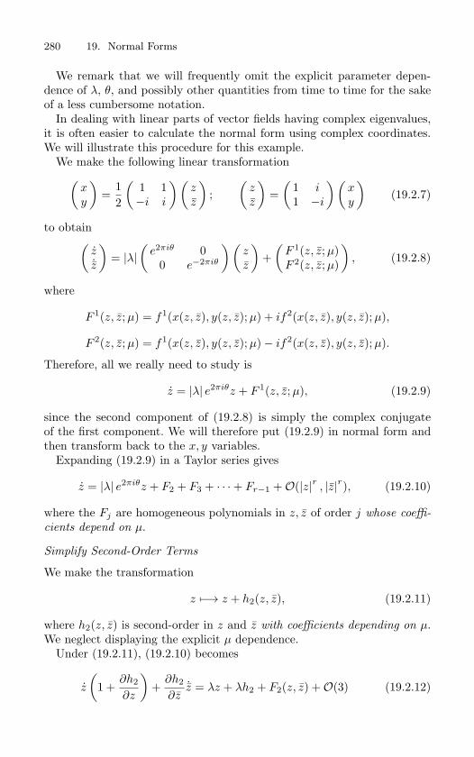
280 19. Normal Forms
We remark that we will frequently omit the explicit parameter depen-dence of λ, θ, and possibly other quantities from time to time for the sakeof a less cumbersome notation.
In dealing with linear parts of vector fields having complex eigenvalues,it is often easier to calculate the normal form using complex coordinates.We will illustrate this procedure for this example.
We make the following linear transformation(xy
)=
12
(1 1−i i
)(zz
);
(zz
)=
(1 i1 −i
)(xy
)(19.2.7)
to obtain(z˙z
)= |λ|
(e2πiθ 0
0 e−2πiθ
)(zz
)+
(F 1(z, z; µ)F 2(z, z; µ)
), (19.2.8)
where
F 1(z, z; µ) = f1(x(z, z), y(z, z);µ) + if2(x(z, z), y(z, z);µ),
F 2(z, z; µ) = f1(x(z, z), y(z, z);µ)− if2(x(z, z), y(z, z);µ).
Therefore, all we really need to study is
z = |λ| e2πiθz + F 1(z, z;µ), (19.2.9)
since the second component of (19.2.8) is simply the complex conjugateof the first component. We will therefore put (19.2.9) in normal form andthen transform back to the x, y variables.
Expanding (19.2.9) in a Taylor series gives
z = |λ| e2πiθz + F2 + F3 + · · ·+ Fr−1 +O(|z|r , |z|r), (19.2.10)
where the Fj are homogeneous polynomials in z, z of order j whose coeffi-
cients depend on µ.
Simplify Second-Order Terms
We make the transformation
z −→ z + h2(z, z), (19.2.11)
where h2(z, z) is second-order in z and z with coefficients depending on µ.We neglect displaying the explicit µ dependence.
Under (19.2.11), (19.2.10) becomes
z
(1 +
∂h2
∂z
)+
∂h2
∂z˙z = λz + λh2 + F2(z, z) +O(3) (19.2.12)
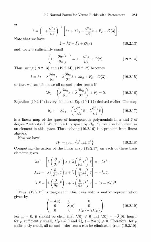
19.2 Normal Forms for Vector Fields with Parameters 281
or
z =(
1 +∂h2
∂z
)−1 [λz + λh2 −
∂h2
∂z˙z + F2 +O(3)
].
Note that we have˙z = λz + F2 +O(3) (19.2.13)
and, for z, z sufficiently small(1 +
∂h2
∂z
)−1
= 1− ∂h2
∂z+O(2). (19.2.14)
Thus, using (19.2.13) and (19.2.14), (19.2.12) becomes
z = λz − λ∂h2
∂zz − λ
∂h2
∂zz + λh2 + F2 +O(3), (19.2.15)
so that we can eliminate all second-order terms if
λh2 −(
λ∂h2
∂zz + λ
∂h2
∂zz
)+ F2 = 0. (19.2.16)
Equation (19.2.16) is very similar to Eq. (19.1.17) derived earlier. The map
h2 −→ λh2 −(
λ∂h2
∂zz + λ
∂h2
∂zz
)(19.2.17)
is a linear map of the space of homogeneous polynomials in z and z ofdegree 2 into itself. We denote this space by H2. F2 can also be viewed asan element in this space. Thus, solving (19.2.16) is a problem from linearalgebra.
Now we haveH2 = span
z2, zz, z2 . (19.2.18)
Computing the action of the linear map (19.2.17) on each of these basiselements gives
λz2 −[λ
(∂
∂zz2
)z + λ
(∂
∂zz2
)z
]= −λz2,
λzz −[λ
(∂
∂zzz
)z + λ
(∂
∂zzz
)z
]= −λzz,
λz2 −[λ
(∂
∂zz2
)z + λ
(∂
∂zz2
)z
]= (λ− 2λ)z2.
Thus, (19.2.17) is diagonal in this basis with a matrix representationgiven by
−λ(µ) 0 00 −λ(µ) 00 0 λ(µ)− 2λ(µ)
. (19.2.19)
For µ = 0, it should be clear that λ(0) = 0 and λ(0) = −λ(0); hence,for µ sufficiently small, λ(µ) = 0 and λ(µ) − 2λ(µ) = 0. Therefore, for µsufficiently small, all second-order terms can be eliminated from (19.2.10).
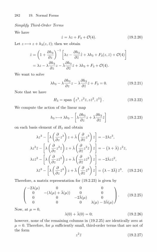
282 19. Normal Forms
Simplify Third-Order Terms
We havez = λz + F3 +O(4). (19.2.20)
Let z −→ z + h3(z, z); then we obtain
z =(
1 +∂h3
∂z
)−1 [λz − ∂h3
∂z˙z + λh3 + F3(z, z) +O(4)
]
= λz − λ∂h3
∂zz − λ
∂h3
∂zz + λh3 + F3 +O(4).
We want to solve
λh3 − λ∂h3
∂zz − λ
∂h3
∂zz + F3 = 0. (19.2.21)
Note that we have
H3 = spanz3, z2z, zz2, z3 . (19.2.22)
We compute the action of the linear map
h3 −→ λh3 −[λ
∂h3
∂zz + λ
∂h3
∂zz
](19.2.23)
on each basis element of H3 and obtain
λz3 −[λ
(∂
∂zz3
)z + λ
(∂
∂zz3
)z
]= −2λz3,
λz2z −[λ
(∂
∂zz2z
)z + λ
(∂
∂zz2z
)z
]= −
(λ + λ
)z2z,
λzz2 −[λ
(∂
∂zzz2
)z + λ
(∂
∂zzz2
)z
]= −2λzz2,
λz3 −[λ
(∂
∂zz3
)z + λ
(∂
∂zz3
)z
]=
(λ− 3λ
)z3. (19.2.24)
Therefore, a matrix representation for (19.2.23) is given by−2λ(µ) 0 0 0
0 −(λ(µ) + λ(µ)) 0 00 0 −2λ(µ) 00 0 0 λ(µ)− 3λ(µ)
. (19.2.25)
Now, at µ = 0,λ(0) + λ(0) = 0; (19.2.26)
however, none of the remaining columns in (19.2.25) are identically zero atµ = 0. Therefore, for µ sufficiently small, third-order terms that are not ofthe form
z2z (19.2.27)
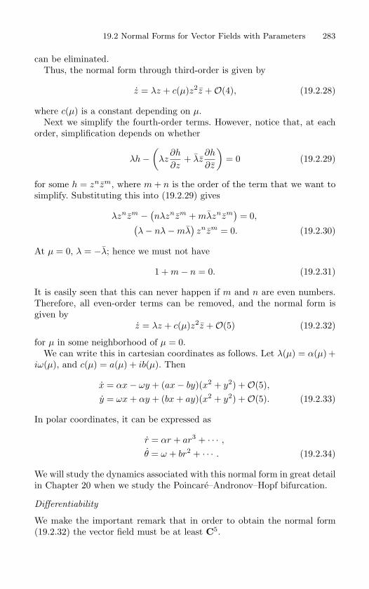
19.2 Normal Forms for Vector Fields with Parameters 283
can be eliminated.Thus, the normal form through third-order is given by
z = λz + c(µ)z2z +O(4), (19.2.28)
where c(µ) is a constant depending on µ.Next we simplify the fourth-order terms. However, notice that, at each
order, simplification depends on whether
λh−(
λz∂h
∂z+ λz
∂h
∂z
)= 0 (19.2.29)
for some h = znzm, where m + n is the order of the term that we want tosimplify. Substituting this into (19.2.29) gives
λznzm −(nλznzm + mλznzm
)= 0,(
λ− nλ−mλ)znzm = 0. (19.2.30)
At µ = 0, λ = −λ; hence we must not have
1 + m− n = 0. (19.2.31)
It is easily seen that this can never happen if m and n are even numbers.Therefore, all even-order terms can be removed, and the normal form isgiven by
z = λz + c(µ)z2z +O(5) (19.2.32)
for µ in some neighborhood of µ = 0.We can write this in cartesian coordinates as follows. Let λ(µ) = α(µ) +
iω(µ), and c(µ) = a(µ) + ib(µ). Then
x = αx− ωy + (ax− by)(x2 + y2) +O(5),y = ωx + αy + (bx + ay)(x2 + y2) +O(5). (19.2.33)
In polar coordinates, it can be expressed as
r = αr + ar3 + · · · ,
θ = ω + br2 + · · · . (19.2.34)
We will study the dynamics associated with this normal form in great detailin Chapter 20 when we study the Poincare–Andronov–Hopf bifurcation.
Differentiability
We make the important remark that in order to obtain the normal form(19.2.32) the vector field must be at least C5.
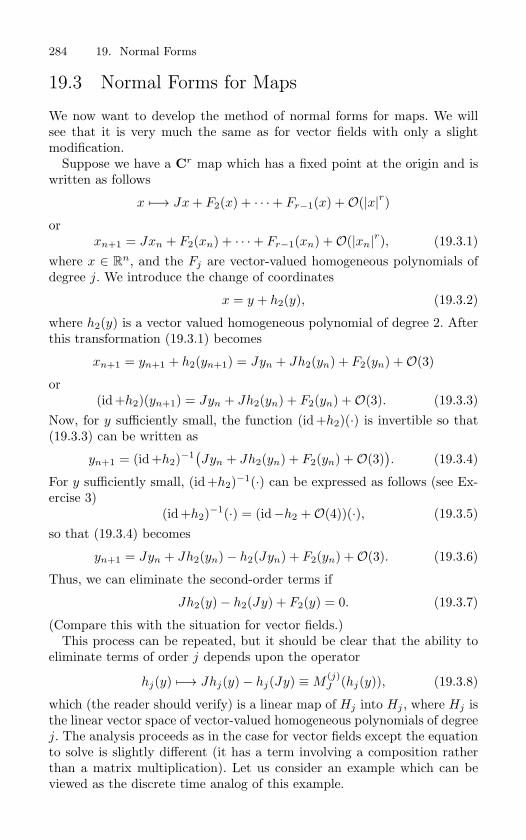
284 19. Normal Forms
19.3 Normal Forms for Maps
We now want to develop the method of normal forms for maps. We willsee that it is very much the same as for vector fields with only a slightmodification.
Suppose we have a Cr map which has a fixed point at the origin and iswritten as follows
x −→ Jx + F2(x) + · · ·+ Fr−1(x) +O(|x|r)or
xn+1 = Jxn + F2(xn) + · · ·+ Fr−1(xn) +O(|xn|r), (19.3.1)where x ∈ R
n, and the Fj are vector-valued homogeneous polynomials ofdegree j. We introduce the change of coordinates
x = y + h2(y), (19.3.2)
where h2(y) is a vector valued homogeneous polynomial of degree 2. Afterthis transformation (19.3.1) becomes
xn+1 = yn+1 + h2(yn+1) = Jyn + Jh2(yn) + F2(yn) +O(3)
or(id +h2)(yn+1) = Jyn + Jh2(yn) + F2(yn) +O(3). (19.3.3)
Now, for y sufficiently small, the function (id +h2)(·) is invertible so that(19.3.3) can be written as
yn+1 = (id +h2)−1(Jyn + Jh2(yn) + F2(yn) +O(3)). (19.3.4)
For y sufficiently small, (id +h2)−1(·) can be expressed as follows (see Ex-ercise 3)
(id +h2)−1(·) = (id−h2 +O(4))(·), (19.3.5)so that (19.3.4) becomes
yn+1 = Jyn + Jh2(yn)− h2(Jyn) + F2(yn) +O(3). (19.3.6)
Thus, we can eliminate the second-order terms if
Jh2(y)− h2(Jy) + F2(y) = 0. (19.3.7)
(Compare this with the situation for vector fields.)This process can be repeated, but it should be clear that the ability to
eliminate terms of order j depends upon the operator
hj(y) −→ Jhj(y)− hj(Jy) ≡ M(j)J (hj(y)), (19.3.8)
which (the reader should verify) is a linear map of Hj into Hj , where Hj isthe linear vector space of vector-valued homogeneous polynomials of degreej. The analysis proceeds as in the case for vector fields except the equationto solve is slightly different (it has a term involving a composition ratherthan a matrix multiplication). Let us consider an example which can beviewed as the discrete time analog of this example.
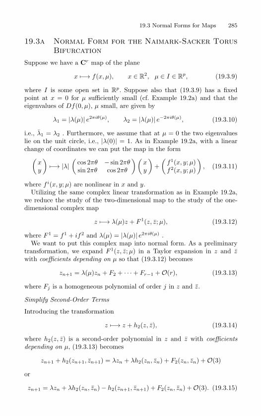
19.3 Normal Forms for Maps 285
19.3a Normal Form for the Naimark-Sacker TorusBifurcation
Suppose we have a Cr map of the plane
x −→ f(x, µ), x ∈ R2, µ ∈ I ∈ R
p, (19.3.9)
where I is some open set in Rp. Suppose also that (19.3.9) has a fixed
point at x = 0 for µ sufficiently small (cf. Example 19.2a) and that theeigenvalues of Df(0, µ), µ small, are given by
λ1 = |λ(µ)| e2πiθ(µ), λ2 = |λ(µ)| e−2πiθ(µ), (19.3.10)
i.e., λ1 = λ2 . Furthermore, we assume that at µ = 0 the two eigenvalueslie on the unit circle, i.e., |λ(0)| = 1. As in Example 19.2a, with a linearchange of coordinates we can put the map in the form(
xy
)−→ |λ|
(cos 2πθ − sin 2πθsin 2πθ cos 2πθ
)(xy
)+
(f1(x, y;µ)f2(x, y;µ)
), (19.3.11)
where f i(x, y;µ) are nonlinear in x and y.Utilizing the same complex linear transformation as in Example 19.2a,
we reduce the study of the two-dimensional map to the study of the one-dimensional complex map
z −→ λ(µ)z + F 1(z, z; µ), (19.3.12)
where F 1 = f1 + if2 and λ(µ) = |λ(µ)| e2πiθ(µ) .We want to put this complex map into normal form. As a preliminary
transformation, we expand F 1(z, z; µ) in a Taylor expansion in z and zwith coefficients depending on µ so that (19.3.12) becomes
zn+1 = λ(µ)zn + F2 + · · ·+ Fr−1 +O(r), (19.3.13)
where Fj is a homogeneous polynomial of order j in z and z.
Simplify Second-Order Terms
Introducing the transformation
z −→ z + h2(z, z), (19.3.14)
where h2(z, z) is a second-order polynomial in z and z with coefficients
depending on µ, (19.3.13) becomes
zn+1 + h2(zn+1, zn+1) = λzn + λh2(zn, zn) + F2(zn, zn) +O(3)
or
zn+1 = λzn + λh2(zn, zn)− h2(zn+1, zn+1) + F2(zn, zn) +O(3). (19.3.15)
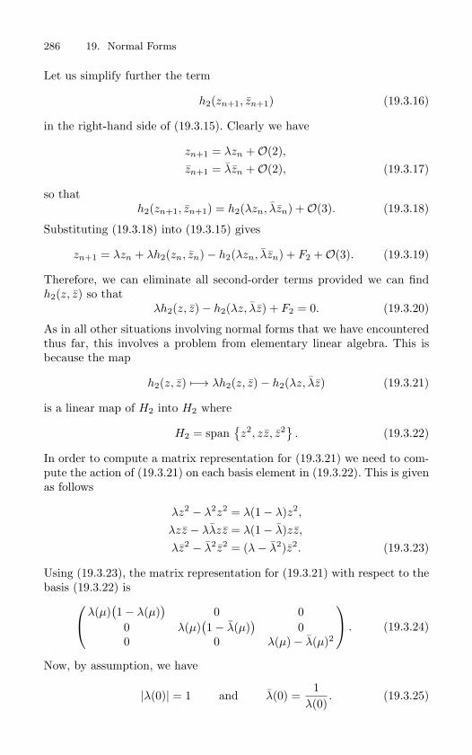
286 19. Normal Forms
Let us simplify further the term
h2(zn+1, zn+1) (19.3.16)
in the right-hand side of (19.3.15). Clearly we have
zn+1 = λzn +O(2),zn+1 = λzn +O(2), (19.3.17)
so thath2(zn+1, zn+1) = h2(λzn, λzn) +O(3). (19.3.18)
Substituting (19.3.18) into (19.3.15) gives
zn+1 = λzn + λh2(zn, zn)− h2(λzn, λzn) + F2 +O(3). (19.3.19)
Therefore, we can eliminate all second-order terms provided we can findh2(z, z) so that
λh2(z, z)− h2(λz, λz) + F2 = 0. (19.3.20)
As in all other situations involving normal forms that we have encounteredthus far, this involves a problem from elementary linear algebra. This isbecause the map
h2(z, z) −→ λh2(z, z)− h2(λz, λz) (19.3.21)
is a linear map of H2 into H2 where
H2 = spanz2, zz, z2 . (19.3.22)
In order to compute a matrix representation for (19.3.21) we need to com-pute the action of (19.3.21) on each basis element in (19.3.22). This is givenas follows
λz2 − λ2z2 = λ(1− λ)z2,
λzz − λλzz = λ(1− λ)zz,
λz2 − λ2z2 = (λ− λ2)z2. (19.3.23)
Using (19.3.23), the matrix representation for (19.3.21) with respect to thebasis (19.3.22) is
λ(µ)(1− λ(µ)
)0 0
0 λ(µ)(1− λ(µ)
)0
0 0 λ(µ)− λ(µ)2
. (19.3.24)
Now, by assumption, we have
|λ(0)| = 1 and λ(0) =1
λ(0). (19.3.25)
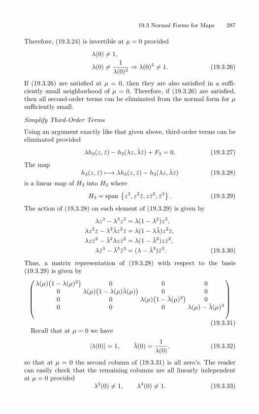
19.3 Normal Forms for Maps 287
Therefore, (19.3.24) is invertible at µ = 0 provided
λ(0) = 1,
λ(0) = 1λ(0)2
⇒ λ(0)3 = 1. (19.3.26)
If (19.3.26) are satisfied at µ = 0, then they are also satisfied in a suffi-ciently small neighborhood of µ = 0. Therefore, if (19.3.26) are satisfied,then all second-order terms can be eliminated from the normal form for µsufficiently small.
Simplify Third-Order Terms
Using an argument exactly like that given above, third-order terms can beeliminated provided
λh3(z, z)− h3(λz, λz) + F3 = 0. (19.3.27)
The maph3(z, z) −→ λh3(z, z)− h3(λz, λz) (19.3.28)
is a linear map of H3 into H3 where
H3 = spanz3, z2z, zz2, z3 . (19.3.29)
The action of (19.3.28) on each element of (19.3.29) is given by
λz3 − λ3z3 = λ(1− λ2)z3,
λz2z − λ2λz2z = λ(1− λλ)z2z,
λzz2 − λ2λzz2 = λ(1− λ2)zz2,
λz3 − λ3z3 = (λ− λ3)z3. (19.3.30)
Thus, a matrix representation of (19.3.28) with respect to the basis(19.3.29) is given by
λ(µ)(1− λ(µ)2
)0 0 0
0 λ(µ)(1− λ(µ)λ(µ)
)0 0
0 0 λ(µ)(1− λ(µ)2
)0
0 0 0 λ(µ)− λ(µ)3
(19.3.31)Recall that at µ = 0 we have
|λ(0)| = 1, λ(0) =1
λ(0), (19.3.32)
so that at µ = 0 the second column of (19.3.31) is all zero’s. The readercan easily check that the remaining columns are all linearly independentat µ = 0 provided
λ2(0) = 1, λ4(0) = 1. (19.3.33)
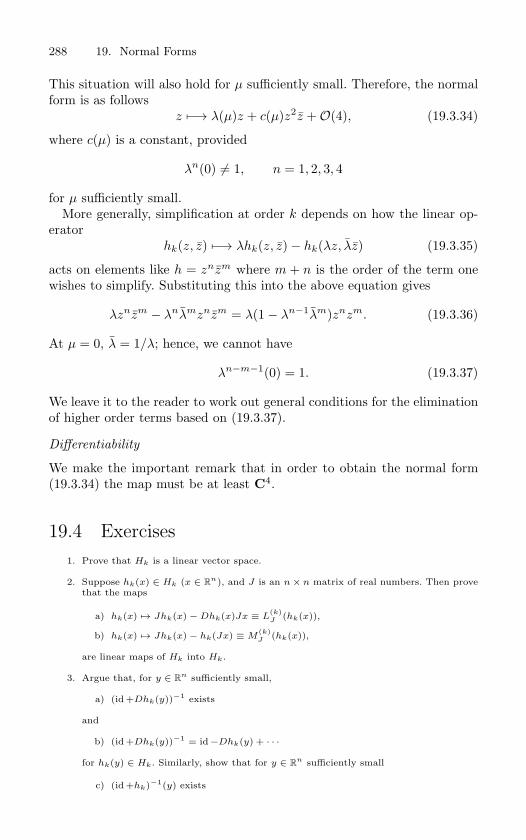
288 19. Normal Forms
This situation will also hold for µ sufficiently small. Therefore, the normalform is as follows
z −→ λ(µ)z + c(µ)z2z +O(4), (19.3.34)
where c(µ) is a constant, provided
λn(0) = 1, n = 1, 2, 3, 4
for µ sufficiently small.More generally, simplification at order k depends on how the linear op-
eratorhk(z, z) −→ λhk(z, z)− hk(λz, λz) (19.3.35)
acts on elements like h = znzm where m + n is the order of the term onewishes to simplify. Substituting this into the above equation gives
λznzm − λnλmznzm = λ(1− λn−1λm)znzm. (19.3.36)
At µ = 0, λ = 1/λ; hence, we cannot have
λn−m−1(0) = 1. (19.3.37)
We leave it to the reader to work out general conditions for the eliminationof higher order terms based on (19.3.37).
Differentiability
We make the important remark that in order to obtain the normal form(19.3.34) the map must be at least C4.
19.4 Exercises1. Prove that Hk is a linear vector space.
2. Suppose hk(x) ∈ Hk (x ∈ Rn), and J is an n × n matrix of real numbers. Then prove
that the maps
a) hk(x) → Jhk(x) − Dhk(x)Jx ≡ L(k)J (hk(x)),
b) hk(x) → Jhk(x) − hk(Jx) ≡ M(k)J (hk(x)),
are linear maps of Hk into Hk.
3. Argue that, for y ∈ Rn sufficiently small,
a) (id +Dhk(y))−1 exists
and
b) (id +Dhk(y))−1 = id −Dhk(y) + · · ·
for hk(y) ∈ Hk. Similarly, show that for y ∈ Rn sufficiently small
c) (id +hk)−1(y) exists
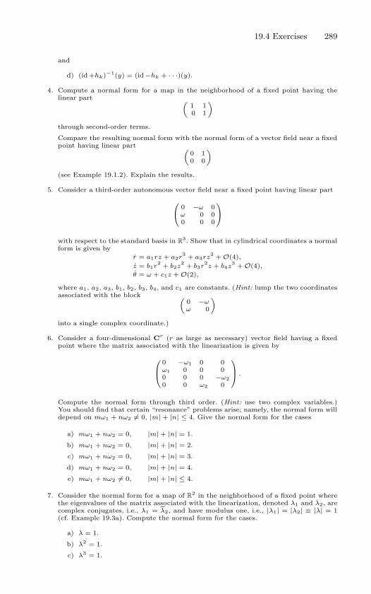
19.4 Exercises 289
and
d) (id +hk)−1(y) = (id −hk + · · ·)(y).
4. Compute a normal form for a map in the neighborhood of a fixed point having thelinear part (
1 10 1
)
through second-order terms.
Compare the resulting normal form with the normal form of a vector field near a fixedpoint having linear part (
0 10 0
)
(see Example 19.1.2). Explain the results.
5. Consider a third-order autonomous vector field near a fixed point having linear part
0 −ω 0
ω 0 00 0 0
with respect to the standard basis in R3. Show that in cylindrical coordinates a normal
form is given byr = a1rz + a2r
3 + a3rz2 + O(4),
z = b1r2 + b2z
2 + b3r2z + b4z
3 + O(4),θ = ω + c1z + O(2),
where a1, a2, a3, b1, b2, b3, b4, and c1 are constants. (Hint: lump the two coordinatesassociated with the block (
0 −ωω 0
)
into a single complex coordinate.)
6. Consider a four-dimensional Cr (r as large as necessary) vector field having a fixedpoint where the matrix associated with the linearization is given by
0 −ω1 0 0ω1 0 0 00 0 0 −ω20 0 ω2 0
.
Compute the normal form through third order. (Hint: use two complex variables.)You should find that certain “resonance” problems arise; namely, the normal form willdepend on mω1 + nω2 = 0, |m| + |n| ≤ 4. Give the normal form for the cases
a) mω1 + nω2 = 0, |m| + |n| = 1.
b) mω1 + nω2 = 0, |m| + |n| = 2.
c) mω1 + nω2 = 0, |m| + |n| = 3.
d) mω1 + nω2 = 0, |m| + |n| = 4.
e) mω1 + nω2 = 0, |m| + |n| ≤ 4.
7. Consider the normal form for a map of R2 in the neighborhood of a fixed point where
the eigenvalues of the matrix associated with the linearization, denoted λ1 and λ2, arecomplex conjugates, i.e., λ1 = λ2, and have modulus one, i.e., |λ1| = |λ2| ≡ |λ| = 1(cf. Example 19.3a). Compute the normal form for the cases.
a) λ = 1.
b) λ2 = 1.
c) λ3 = 1.
290 19. Normal Forms
d) λ4 = 1.
8. Compute the normal form of a map of R2 in the neighborhood of a fixed point where
the matrix associated with the linearization has the following form
a)(
1 10 1
).
b)(
1 00 1
).
c)(
−1 10 −1
).
d)(
−1 00 −1
).
Compare your normal forms with those obtained in parts a) and b) of Exercise 7.
9. Consider a Cr (r ≥ 2) vector field
x = f(x, µ), x ∈ R2, µ ∈ R
1,
defined on a sufficiently large open set in R2 × R
1. Suppose that (x, µ) = (0, 0) isa fixed point of this vector field and that Dxf(0, 0) has a pair of purely imaginaryeigenvalues.
a) Show that there exists a curve of fixed points of the vector field, denoted x(µ),x(0) = 0, for µ sufficiently small.
b) By using this curve of fixed points as a parameter-dependent coordinate trans-formation, show that one can choose coordinates so that the origin in phasespace remains a fixed point for µ sufficiently small.
19.5 The Elphick-Tirapegui-Brachet-Coullet-IoossNormal Form
In this section we will describe the work of Elphick et al. [1987]. A keyfeature of their work is that they introduce an inner product on Hk. Thisinner product can be used to construct the orthogonal complement to L
(k)J .
The resulting normal form has a number of nice properties. Moreover, theirmethod seems to be computationally very efficient. Similar work by Cush-man and Sanders [1986] appeared simultaneously, however all of the resultsdescribed in this section are taken from Elphick et al. [1987].
For easier reference we recall (19.1.8), which we wish to transform intonormal form:
x = Jx + F2(x) + F3(x) + · · ·+ Fr−1(x) +O(|x|r),≡ Jx + F(x) +O(|x|r), (19.5.1)
where Fi(x) represent the order i terms in the Taylor expansion of F (x)and F(x) represents the nonlinear terms in this expansion through orderr − 1.
19.5 The Elphick-Tirapegui-Brachet-Coullet-Iooss Normal Form 291
19.5a An Inner Product on Hk
First we define an inner product on the scalar valued homogeneous polyno-mials of degree k, and then use this to construct an inner product on Hk.Let x = (x1, . . . , xn) and let p(x), q(x) denote scalar valued homogeneouspolynomials in x of degree k. For example,
p(x) =∑
m1+···+mn=k
mi∈ZZ+∪0
am1···mnxm1
1 · · ·xmnn , (19.5.2)
where ZZ+ denotes the positive integers, and am1···mndenotes a scalar.
Following Bargmann [1961], Elphick et al. [1987] define the following innerproduct on the space of scalar valued homogeneous polynomials in x ofdegree k
〈p, q〉 ≡ p(∂)q(x)|x=0, (19.5.3)
where p(∂) is the symbol for a homogeneous polynomial of degree k in(∂1, · · · , ∂n) with ∂i ≡ ∂
∂xi. For example, for p(x) as defined in (19.5.2), we
havep(∂) =
∑m1+···+mn=k
mi∈ZZ+∪0
am1···mn
∂m1
∂xm11· · · ∂mn
∂xmnn
. (19.5.4)
The following example computation is instructive. Let
p(x) = xm11 · · ·xmn
n , q(x) = xm11 · · ·xmn
n ,n∑
i=1
mi =n∑
i=1
mi.
Then
〈p, q〉 =(
∂m1
∂xm11· · · ∂mn
∂xmnn
)(xm1
1 · · ·xmnn
)=
n∏i=1
∂mi
∂xmii
xmii =
n∏i=1
δmi,mimi!.
There are two basic properties of this inner product that we now derive.
Property One
Let p(x), q(x), r(x) denote scalar valued homogeneous polynomials in x ofdegree k. Then it follows from (19.5.3) that
〈qr, p〉 = q(∂)r(∂)p(x)|x=0,
= r(∂)q(∂)p(x)|x=0,
= 〈r, q(∂)p〉. (19.5.5)
This equation states that multiplication by the polynomial q(x) is the ad-joint of differentiation by q(∂).
292 19. Normal Forms
Property Two
Another key property is the following.Suppose A : R
n → Rn is a linear, invertible operator. Then the second
basic property is the following
〈p(Ax), q(x)〉 = 〈p(x), q(A∗x)〉, (19.5.6)
where A∗ denotes the adjoint of A. We will leave the proof of this propertyto the exercises.
Now we construct an inner product on Hk. With respect to the chosenbasis on R
n, the corresponding coordinates of a point x ∈ Rn are denoted
x = (x1, . . . , xn). Then, with respect to this same basis, a vector valuedhomogeneous polynomial of degree k (i.e., an element of Hk) is denotedhk(x) =
(h1
k(x), . . . , hnk (x)
), where hi
k(x) is a scalar valued homogeneouspolynomial of degree k for each i. Then an inner product on Hk is defined asfollows. For hk, gk ∈ Hk, the inner product of these two vectors is definedby
〈hk, gk〉Hk=
n∑i=1
〈hik, gi
k〉. (19.5.7)
Since we are dealing with real vector fields note that A∗ is the adjoint
with respect to the standard Euclidean inner product on Rn, i.e., it is
the transpose of A, denoted AT . We could have just as easily developed
the theory for vector fields on Cn. In that case A∗ would be the adjoint
with respect to the usual inner product on Cn. Then the inner product
(19.5.3) would be modified as follows:
〈p, q〉 ≡ p(∂)q(x)|x=0.
The complex case will be useful when we have imaginary eigenvalues
and perform calculations using the complexification of the real case.
19.5b The Main TheoremsWith this inner product in hand, we can now prove the main results thatdescribe the structure of the normal form.
Suppose hk, gk ∈ Hk and A : Rn → R
n is a linear invertible operator.Then
〈A−1gk (Ax) , hk (x)〉Hk= 〈gk (Ax) , A∗−1hk (x)〉Hk
,
= 〈gk (x) , A∗−1 (hk (A∗x))〉Hk, using (19.5.6).
(19.5.8)
In (19.5.8) substitute A = eJt. Then (19.5.8) becomes
〈e−Jtgk
(eJtx
), hk (x)〉Hk
= 〈gk (x) , e−J∗thk
(eJ∗tx
)〉Hk
, (19.5.9)
19.5 The Elphick-Tirapegui-Brachet-Coullet-Iooss Normal Form 293
where we have used(eJt
)∗ = eJ∗t. Next we differentiate (19.5.9) withrespect to t and evaluate the result at t = 0 to obtain
〈−Jgk(x) + Dgk(x)Jx, hk(x)〉Hk= 〈gk(x),−J∗hk(x) + Dhk(x)J∗x〉Hk
,(19.5.10)
or, using the notation developed in (19.1.23) and (19.1.24),
〈[gk, Jx] , hk〉Hk= 〈gk, [hk, J∗x]〉Hk
, (19.5.11)
or〈L(k)
J (gk) , hk〉Hk= 〈gk, L
(k)J∗ (hk)〉Hk
, (19.5.12)
from which it follows that (L
(k)J
)∗= L
(k)J∗ .
But most importantly, this expression implies that if hk ∈ Ker L(k)J∗ then
hk is in the orthogonal complement of the image of L(k)J , denoted Im L
(k)J .
This is a key feature of the normal form, but before summarizing this in atheorem we want to develop a useful characterization of Ker L
(k)J∗ .
First, we argue that
eL(k)J∗ thk(x) = e−J∗thk
(eJ∗tx
). (19.5.13)
This can be seen as follows. Consider the following linear ordinary differ-ential equation on Hk:
hk = L(k)J∗ hk, hk ∈ Hk.
It is a straightforward calculation to verify that
mk(t) = e−J∗thk
(eJ∗tx
),
nk(t) = eL(k)J∗ thk(x),
are both solutions of this equation satisfying
mk(0) = hk(x),nk(0) = hk(x).
Hence, by existence and uniqueness of solutions of linear ordinary differen-tial equations with constant coefficients, it follows that mk(t) = nk(t) forall t. Therefore (19.5.13) holds.
Now eL(k)J∗ t acts as the identity map on KerL
(k)J∗ . Hence it follows that
Ker L(k)J∗ =
hk ∈ Hk | e−J∗thk
(eJ∗tx
)= hk(x), ∀t ∈ R
. (19.5.14)
We can summarize these results in the following theorem.
294 19. Normal Forms
Theorem 19.5.1 (Elphick-Tirapegui-Brachet-Coullet-Iooss) Hk can
be decomposed as follows:
Hk = ImL(k)J ⊕KerL
(k)J∗ ,
where
KerL(k)J∗ =
hk ∈ Hk | e−J∗thk
(eJ∗tx
)= hk(x), ∀t ∈ R
.
Applying this result to successive orders of the Taylor expansion of(19.5.1), we can immediately state a theorem characterizing what we meanby the normal form of (19.5.1)
Theorem 19.5.2 (Elphick-Tirapegui-Brachet-Coullet-Iooss) The
vector field (19.5.1) is said to be in normal form through order r− 1 if the
nonlinear terms F(x) commutes with eJ∗t is the sense that
e−J∗tF(eJ∗tx
)= F(x). (19.5.15)
Or, equivalently, if F(x) satisfies the following partial differential equation
DF(x)J∗x− J∗F(x) = 0. (19.5.16)
Note that the partial differential equation (19.5.16) can be solved by themethod of characteristics. Writing (19.5.16) out in components gives
n∑j,l=1
∂Fi
∂xjJljxl −
n∑j=1
JjiFj = 0, i = 1, . . . , n. (19.5.17)
The characteristic system associated with (19.5.17) is given by
dxj∑l Jljxl
=dFi∑l JliFl
, i, j = 1, . . . , n. (19.5.18)
It follows immediately that the characteristic curves in Rn are given by
x(t) = eJ∗tx0. (19.5.19)
This result is useful for giving another characterization of the nonlinearterms of the normal form.
Theorem 19.5.3 (Elphick-Tirapegui-Brachet-Coullet-Iooss) The
nonlinear terms of the normal form can be written in the following form:
F(x) =n∑
i=1
αj(x)Lix, (19.5.20)
where Li, i = 1, . . . , n are linear operators commuting with J∗ in Rn (to
be explicitly constructed in the proof), and the scalar functions αi(x), i =1, . . . , n, are rational functions that are first integrals of the characteristic
system x = J∗x.
19.5 The Elphick-Tirapegui-Brachet-Coullet-Iooss Normal Form 295
Proof: First we construct the linear operators L1, . . . ,Ln. To do this, we willassume that J∗ is in Jordan canonical form. Then it has r Jordan blocks,with each block J∗
j corresponding to an invariant subspace of Rn, denoted
Ej , and to an eigenvalue λj , j = 1, . . . , r. Let νj denote the dimension ofEj and Pj denote the projection onto Ej . Then
r∑i=1
Pj = id.
To each Jordan block we associate νj linear operators
Pj ,(J∗
j − λj id)Pj , . . . ,
(J∗
j − λj id)νj−1
Pj , j = 1, . . . , r.
This is a set of n linearly independent operators, with each commuting withJ∗, which we denote by Lj . Now we choose any x ∈ R
n having the propertythat it has a nonzero component in each of the Ej . Then Ljx, j = 1, . . . , nforms a basis for R
n. We express F(x) in this basis to obtain (19.5.20).Next we examine the properties of the coefficients in this expansion, αj(x).
SinceJ∗Lj = LjJ
∗, j = 1, . . . , n,
it follows thateJ∗tLj = Lje
J∗t, j = 1, . . . , n. (19.5.21)
Now using (19.5.15), we obtain
e−J∗tF(eJ∗tx
)=
n∑j=1
e−J∗tαj
(eJ∗tx
)Lje
J∗tx,
=n∑
j=1
e−J∗tαj
(eJ∗tx
)eJ∗tLjx,
=n∑
j=1
αj
(eJ∗tx
)Ljx,
= F(x) =n∑
j=1
αj(x)Ljx.
Henceαj
(eJ∗tx
)= αj(x). (19.5.22)
Therefore the functions αj(x) are first integrals of the characteristic system.
296 19. Normal Forms
19.5c Symmetries of the Normal FormSuppose T : R
n → Rn is a linear invertible operator. Consider an arbitrary
vector fieldx = f(x), x ∈ R
n. (19.5.23)
We say that T is a symmetry of (19.5.23) if
f(Tx) = Tf(x). (19.5.24)
If (19.5.23) has an equilibrium point at x = 0, and J is the matrix associ-ated with the linearization about this equilibrium, then by differentiating(19.5.24) we obtain
JT = TJ. (19.5.25)
The terminology “T commutes with the vector field” is also used.From our construction of the normal form we see immediately that the
one-parameter group of transformationseJ∗t, t ∈ R
is a symmetry for
the normal form. In this section we will prove that if the vector field has anadditional symmetry, denoted by the linear invertible operator T : R
n →R
n, then the normal form as constructed above, also has the symmetry T .To begin with, we define the following linear operator on Hk:
T∗hk(x) = T−1hk(Tx), (19.5.26)
which will be useful for proving the following lemma.
Lemma 19.5.4 The image of L(k)J , ImL
(k)J , and the kernel of L
(k)J ,
KerL(k)J , are invariant under T∗.
Proof: First we show that T∗ commutes with L(k)J in the following sense:
L(k)J (T∗hk(x)) = L
(k)J
(T−1hk(Tx)
)= JT−1hk(Tx)−D
(T−1hk(Tx)
)Jx
= JT−1hk(Tx)− T−1Dhk(Tx)TJx
= T−1Jhk(Tx)− T−1Dhk(Tx)JTx
= T−1 (Jhk(Tx)−Dhk(Tx)JTx)
= T−1L(k)J (hk(Tx)) = T∗L
(k)J (hk(x)) ,
(19.5.27)
where in this calculation we have used
JT = TJ ⇒ T−1J = JT−1.
The lemma follows directly from this calculation. Now assume that T is unitary, i.e., T ∗ = T−1. Then we have the following
lemma.
19.5 The Elphick-Tirapegui-Brachet-Coullet-Iooss Normal Form 297
Lemma 19.5.5 The image of L(k)J∗ , ImL
(k)J∗ , and the kernel of L
(k)J∗ ,
KerL(k)J∗ , are invariant under T∗.
Proof: First we show that T∗ commutes with L(k)J∗ in the following sense:
L(k)J∗ (T∗hk(x)) = L
(k)J∗
(T−1hk(Tx)
)= J∗T−1hk(Tx)−D
(T−1hk(Tx)
)J∗x
= J∗T−1hk(Tx)− T−1Dhk(Tx)TJ∗x= T−1J∗hk(Tx)− T−1Dhk(Tx)J∗Tx= T−1 (J∗hk(Tx)−Dhk(Tx)J∗Tx)= T−1L
(k)J∗ (hk(Tx)) = T∗L
(k)j∗ (hk(x)) ,
(19.5.28)
where in this calculation we have used
J∗T = TJ∗ ⇒ T−1J∗ = J∗T−1.
The lemma follows directly from this calculation.
The two lemmas show that both Im L(k)J and KerL
(k)J∗ are invariant under
T∗. We will use these two facts to show that the normal form, as constructedabove, commutes with T .
First, suppose the vector field (19.5.1) has the symmetry T . Then wemust have
x = T−1JTx + T−1F2(Tx) + T−1F3(Tx) + · · · ,= Jx + F2(x) + F3(x) + · · · .
Now we consider simplifying the second order terms. Making the change ofcoordinates
x → x + h2(x),
givesx = Jx + L
(2)J (h2(x)) + F2(x) +O(3),
or
x = Jx + L(2)J (h2(x)) + ΠImL
(2)J F2(x) + ΠKerL
(2)J∗ F2(x) +O(3),
where ΠImL(2)J∗ denotes the projection onto ImL
(2)J and ΠKerL
(2)J∗ denotes
the projection onto KerL(2)J∗ .
We next apply the symmetry transformation to this equation, i.e., we letx → Tx, and act on the equation from the left with T−1 to obtain
x = T−1JTx + T−1L(2)J (h2(Tx)) + T−1ΠImL
(2)J F2(Tx)
+ T−1ΠKerL(2)J∗ F2(Tx) +O(3).
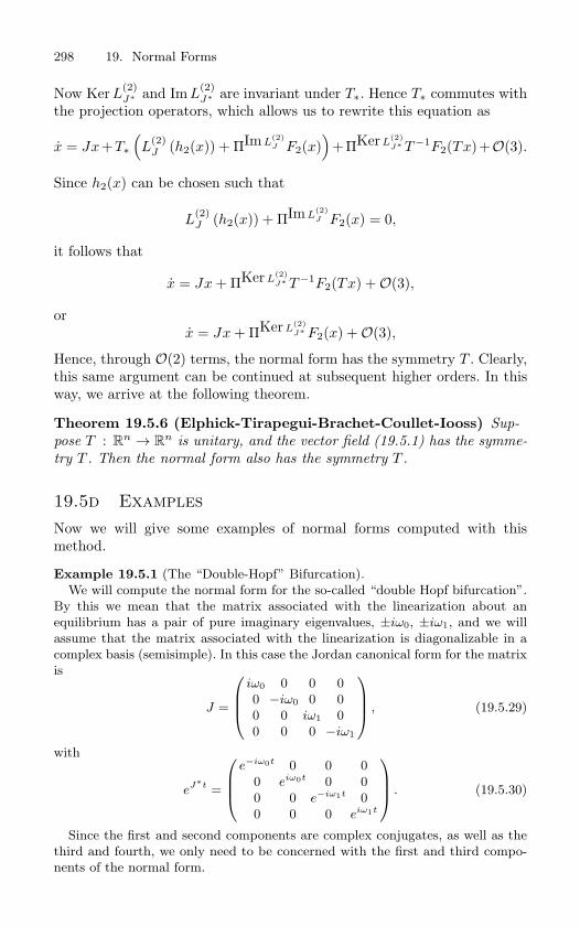
298 19. Normal Forms
Now Ker L(2)J∗ and ImL
(2)J∗ are invariant under T∗. Hence T∗ commutes with
the projection operators, which allows us to rewrite this equation as
x = Jx+T∗(L
(2)J (h2(x)) + ΠImL
(2)J F2(x)
)+ΠKerL
(2)J∗ T−1F2(Tx)+O(3).
Since h2(x) can be chosen such that
L(2)J (h2(x)) + ΠImL
(2)J F2(x) = 0,
it follows that
x = Jx + ΠKerL(2)J∗ T−1F2(Tx) +O(3),
orx = Jx + ΠKerL
(2)J∗ F2(x) +O(3),
Hence, through O(2) terms, the normal form has the symmetry T . Clearly,this same argument can be continued at subsequent higher orders. In thisway, we arrive at the following theorem.
Theorem 19.5.6 (Elphick-Tirapegui-Brachet-Coullet-Iooss) Sup-
pose T : Rn → R
n is unitary, and the vector field (19.5.1) has the symme-
try T . Then the normal form also has the symmetry T .
19.5d ExamplesNow we will give some examples of normal forms computed with thismethod.
Example 19.5.1 (The “Double-Hopf” Bifurcation).
We will compute the normal form for the so-called “double Hopf bifurcation”.
By this we mean that the matrix associated with the linearization about an
equilibrium has a pair of pure imaginary eigenvalues, ±iω0, ±iω1, and we will
assume that the matrix associated with the linearization is diagonalizable in a
complex basis (semisimple). In this case the Jordan canonical form for the matrix
is
J =
iω0 0 0 0
0 −iω0 0 0
0 0 iω1 0
0 0 0 −iω1
, (19.5.29)
with
eJ∗t=
e−iω0t 0 0 0
0 eiω0t 0 0
0 0 e−iω1t 0
0 0 0 eiω1t
. (19.5.30)
Since the first and second components are complex conjugates, as well as the
third and fourth, we only need to be concerned with the first and third compo-
nents of the normal form.
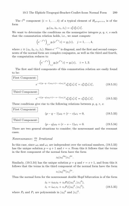
19.5 The Elphick-Tirapegui-Brachet-Coullet-Iooss Normal Form 299
The ith component (i = 1, . . . , 4) of a typical element of Hp+q+r+s is of the
form
gi(z0, z0, z1, z1) = zp0 zq
0zr1 zs
1.
We want to determine the conditions on the nonnegative integers p, q, r, s such
that the commutation relation holds, i.e., we must compute(e−J∗t
)j,i
gi(eJ∗tz) = gj(z), j = 1, . . . , 4,
where z ≡ (z0, z0, z1, z1). Since e−J∗t is diagonal, and the first and second compo-
nents of the normal form are complex conjugates, as well as the third and fourth,
the computation reduces to(e−J∗t
)i,i
gi(eJ∗tz) = gi(z), i = 1, 3.
The first and third components of this commutation relation are easily found
to be:
First Component:
e−i((p−q−1)ω0+(r−s)ω1)tzp0 zq
0zr1 zs
1 = zp0 zq
0zr1 zs
1, (19.5.31)
Third Component:
e−i((p−q)ω0+(r−s−1)ω1)tzp0 zq
0zr1 zs
1 = zp0 zq
0zr1 zs
1. (19.5.32)
These conditions give rise to the following relations between p, q, r, s:
First Component:
(p − q − 1)ω0 + (r − s)ω1 = 0, (19.5.33)
Third Component:
(p − q)ω0 + (r − s − 1)ω1 = 0. (19.5.34)
There are two general situations to consider; the nonresonant and the resonant
cases.
Nonresonance: ω0ω1
Irrational
In this case, since ω0 and ω1 are independent over the rational numbers, (19.5.33)
has the unique solution p = q + 1 and r = s. From this it follows that the terms
in the first component of the normal form have the form
z0|z0|2q|z1|2r.
Similarly, (19.5.34) has the unique solution p = q and r = s + 1, and from this it
follows that the terms in the third component of the normal form have the form
z1|z0|2q|z1|2r.
Thus the normal form for the nonresonant double Hopf bifurcation is of the form
z0 = iω0z0 + z0P0(|z0|2, |z1|2),z1 = iω1z1 + z1P1(|z0|2, |z1|2), (19.5.35)
where P0 and P1 are polynomials in |z0|2 and |z1|2.
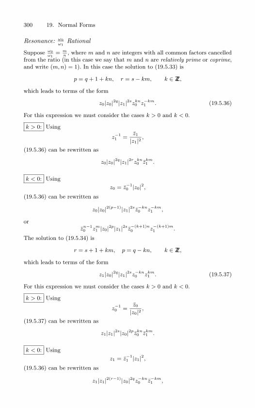
300 19. Normal Forms
Resonance: ω0ω1
Rational
Suppose ω0ω1
= mn
, where m and n are integers with all common factors cancelled
from the ratio (in this case we say that m and n are relatively prime or coprime,and write (m, n) = 1). In this case the solution to (19.5.33) is
p = q + 1 + kn, r = s − km, k ∈ ZZ,
which leads to terms of the form
z0|z0|2q|z1|2szkn0 z−km
1 . (19.5.36)
For this expression we must consider the cases k > 0 and k < 0.
k > 0: Using
z−11 =
z1
|z1|2 ,
(19.5.36) can be rewritten as
z0|z0|2q|z1|2rzkn0 zkm
1 .
k < 0: Using
z0 = z−10 |z0|2,
(19.5.36) can be rewritten as
z0|z0|2(p−1)|z1|2sz−kn0 z−km
1 ,
or
zn−10 zm
1 |z0|2p|z1|2sz−(k+1)n0 z
−(k+1)m1 .
The solution to (19.5.34) is
r = s + 1 + km, p = q − kn, k ∈ ZZ,
which leads to terms of the form
z1|z0|2q|z1|2sz−kn0 zkm
1 . (19.5.37)
For this expression we must consider the cases k > 0 and k < 0.
k > 0: Using
z−10 =
z0
|z0|2 ,
(19.5.37) can be rewritten as
z1|z1|2s|z0|2pzkn0 zkm
1 .
k < 0: Using
z1 = z−11 |z1|2,
(19.5.36) can be rewritten as
z1|z1|2(r−1)|z0|2qz−kn0 z−km
1 ,
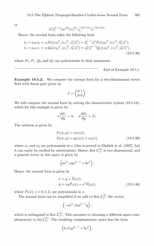
19.5 The Elphick-Tirapegui-Brachet-Coullet-Iooss Normal Form 301
or
zn0 zm−1
1 |z0|2q|z1|2rz−(k+1)n0 z
−(k+1)m1 .
Hence, the normal form takes the following form
z0 = iω0z0 + z0P0(|z0|2, |z1|2, zn0 zm
1 ) + zn−10 zm
1 P1(|z0|2, |z1|2, zn0 zm
1 ),
z1 = iω1z1 + z1Q0(|z0|2, |z1|2, zn0 zm
1 ) + zn0 zm−1
1 Q1(|z0|2, |z1|2, zn0 zm
1 ),
(19.5.38)
where P0, P1, Q0 and Q1 are polynomials in their arguments.
End of Example 19.5.1
Example 19.5.2. We compute the normal form for a two-dimensional vector
field with linear part given by
J =
(0 1
0 0
).
We will compute the normal form by solving the characteristic system (19.5.18),
which for this example is given by
x∂F1
∂y= 0, x
∂F2
∂y= F1.
The solution is given by
F1(x, y) = xφ1(x),
F2(x, y) = yφ1(x) + φ2(x), (19.5.39)
where φ1 and φ2 are polynomials in x (this is proved in Elphick et al. [1987], but
it can easily be verified by substitution). Hence, Ker L(k)J∗ is two dimensional, and
a general vector in this space is given by(axk, ayxk−1
+ bxk)
.
Hence, the normal form is given by
x = y + P0(x),
y = xyP1(x) + x2P2(x), (19.5.40)
where Pi(x), i = 0, 1, 2, are polynomials in x.
The normal form can be simplified if we add to Ker L(k)J∗ the vector(
−axk, kaxk−1y)
,
which is orthogonal to Ker L(k)J∗ . This amounts to choosing a different space com-
plementary to Im L(k)J∗ . The resulting complementary space has the form(
0, a′yxk−1+ bxk
),
302 19. Normal Forms
and the normal form is given by
x = y,
y = xyP1(x) + x2P2(x), (19.5.41)
where P1(x) and P2(x) are polynomials in x.
End of Example 19.5.2
19.5e The Normal Form of a Vector FieldDepending on Parameters
Essentially the same theory goes through for vector fields depending onparameters, but with a few interesting twists.
We rewrite the vector field (19.5.1), where F is O(r − 1) in x:
x = Jx + F(x, µ), x ∈ Rn, µ ∈ R
p, (19.5.42)
with J in Jordan canonical form, and not depending on µ, and
F(0, µ) = O(|µ|), DxF(0, 0) = 0.
Theorem 19.5.7 The vector field (19.5.42) can be transformed to a nor-
mal form in which F(x, µ) satisfies
e−J∗tF(eJ∗tx, µ
)= F(x, µ), (19.5.43)
and
F(0, µ) ∈ KerJ∗, (19.5.44)
J∗DxF(0, µ)−DxF(0, µ)J∗ = 0. (19.5.45)
Proof: The basic idea here, as we mentioned earlier, is that we Taylorexpand in x and view the coefficients as functions of the parameters µ. Inthis way, the previous theory goes through in exactly the same way andthe parameters “just go along for the ride”. However, two new terms doarise in this way, but they cause little difficulty as we will now see.
Taylor expanding (19.5.42) in x gives
x = Jx + F(0, µ) + DxF(0, µ)x +O(|x|2). (19.5.46)
As in the situation with no parameters, we choose the (|x|p) terms to be inKer L
(p)J∗ . In the case with parameters there are two new terms; F(0, µ) ∈ H0
(constant terms) and DxF(0, µ) ∈ H1 (linear terms). Now
L(0)J∗ (F(0, µ)) = J∗F(0, µ) = 0 ⇒ F(0, µ) ∈ Ker J∗,
19.5 The Elphick-Tirapegui-Brachet-Coullet-Iooss Normal Form 303
andL
(1)J∗ (DxF(0, µ)) ⇒ J∗DxF(0, µ)−DxF(0, µ)J∗ = 0.
Requiring the O(|x|p) terms to be in Ker L(p)J∗ , p ≥ 2 immediately leads to
e−J∗tF(eJ∗tx, µ
)= F(x, µ).
This completes the proof of the theorem.
Example 19.5.3.We consider the example of the double-zero eigenvalue with non-semisimple
linear part
J =
(0 1
0 0
),
with the vector field in the form(xy
)= J
(xy
)+
(F1(0, µ)
F2(0, µ)
)+
(F1x(0, µ) F1y(0, µ)
F2x(0, µ) F2y(0, µ)
)(xy
)+ O(|x|2, |y|2).
Then we have (0 0
1 0
)(F1(0, µ)
F2(0, µ)
)=
(0
F1(0, µ)
)⇒ F1(0, µ) = 0,
and(0 0
1 0
)(F1x(0, µ) F1y(0, µ)
F2x(0, µ) F2y(0, µ)
)−
(F1x(0, µ) F1y(0, µ)
F2x(0, µ) F2y(0, µ)
)(0 0
1 0
)=
(0 0
0 0
)⇒ F1y(0, µ) = 0, F1x(0, µ) = F2y(0, µ).
Then the vector field takes the form
x = y + F1x(0, µ)x,
y = F2(0, µ) + F2x(0, µ)x + F1x(0, µ)y + O(|x|2, |y|2).
End of Example 19.5.3
We make some final remarks concerning extensions of the Elphick-Tirapegui-Brachet-Coullet-Iooss approach to normal forsm.
Normal Form for a Vector Field Near a Periodic Orbit
Iooss [1988] has extended the work of Elphick et al. [1987] to the situationof computing the normal form of a vector field in the neighborhood of aperiodic orbit.
Normal Form for a Map Near a Fixed Point
Chen and Della Dora [1999] have extended the work of Elphick et al. [1987]to the situation of computing the normal form of a map near a fixed point.
304 19. Normal Forms
19.6 Exercises1. Prove that
〈p(Ax), q(x)〉 = 〈p(x), q(A∗x)〉.
(Hint: Apply the chain rule and show that ∂x = A∂y where y = A∗x.)
2. Prove that
〈A−1gk (Ax) , hk (x)〉Hk
= 〈gk (x) , A∗−1 (
hk
(A
∗x))
〉Hk.
3. Prove that 〈·, ·〉Hkis an inner product on Hk.
4. Let eini=1 denote the standard basis on R
n and let (x1, . . . , xn) denote coordinateswith respect to this basis. We denote two arbitrary elements of Hk by
hk =n∑
i=1
∑m1+···+mn=k
hik:m1,...,mn
xm11 x
m22 · · · x
mnn ei,
gk =n∑
i=1
∑m1+···+mn=k
gik:m1,...,mn
xm11 x
m22 · · · x
mnn ei.
Compute the inner product of hk and gk.
5. Prove the following result from Elphick et al. [1987]. If J is diagonalizable, then
Ker L(k)J∗ = Ker L
(k)J ,
and the normal form can be constructed so that it commutes with eJt, t ∈ R.
6. Consider a two-dimensional vector field having an equilibrium point at the origin withthe linear part of the vector field given by
J =(
0 10 0
).
Suppose also that the vector field commutes with the linear map defined by the fol-lowing matrix
T =(
−1 00 −1
).
Compute the normal form.
7. Consider a three-dimensional vector field having an equilibrium point at the originwith the linear part of the vector field given by
J =
0 ω 0
−ω 0 00 0 0
,
where ω > 0 is a real number. Suppose also that the vector field commutes with thelinear map defined by the following matrix
T =
1 0 0
0 1 00 0 −1
.
Compute the normal form.
19.6 Exercises 305
8. Consider the non-semisimple double-Hopf bifurcation at 1 : 1 resonance, i.e., a four-dimensional vector field having an equilibrium point at the origin with the linear partof the vector field, with respect to a complex basis, is given by
J =
iω 1 0 00 iω 0 00 0 −iω 10 0 0 −iω
,
where ω > 0 is a real number. Show that in complex coordinates the normal form canbe written as follows
z1 = iωz1 + z2,
z2 = iωz2 + z1φ1 (|z1|, z1z2 − z1z2) + z2φ2 (|z1|, z1z2 − z1z2) ,
where φ1 and φ2 are polynomials in their two arguments.
9. Recall the example of the non-semisimple double-zero eigenvalue depending on pa-rameters. We showed that the normal form could be transformed into the followingform
x = y + F1x(0, µ)x,
y = F2(0, µ) + F2x(0, µ)x + F1x(0, µ)y + +O(|x|2, |y|2).
“Re-parametrize” by letting
F2(0, µ) → µ1,
F1x(0, µ) → µ2,
F2x(0, µ) → µ3.
Show that the µ2x and µ3x term cans be eliminated by appropriate linear transfor-mations.
10. Consider the “double-Hopf bifurcation” as described above, both the resonant and non-resonant cases. Suppose the associated vector field depends on parameters. Computethe terms (19.5.44) and (19.5.45).
11. Consider a two-dimensional vector field having an equilibrium point at the origin withthe linear part of the vector field given by
J =(
0 10 0
).
Suppose also that the vector field commutes with the linear map defined by the fol-lowing matrix
T =(
−1 00 −1
).
Now consider the situation where the vector field depends on parameters. Computethe terms (19.5.44) and (19.5.45).
12. Consider a three-dimensional vector field having an equilibrium point at the originwith the linear part of the vector field given by
J =
0 ω 0
−ω 0 00 0 0
,
where ω > 0 is a real number. Suppose that the vector field depends on parameters.Compute the terms (19.5.44) and (19.5.45).
306 19. Normal Forms
Suppose also that the vector field commutes with the linear map defined by the fol-lowing matrix
T =
1 0 0
0 1 00 0 −1
.
Compute the terms (19.5.44) and (19.5.45).
13. Consider the non-semisimple double-Hopf bifurcation at 1 : 1 resonance, i.e., a four-dimensional vector field having an equilibrium point at the origin with the linear partof the vector field, with respect to a complex basis, is given by
J =
iω 1 0 00 iω 0 00 0 −iω 10 0 0 −iω
,
where ω > 0 is a real number. Suppose that the vector field depends on parametersand compute the terms (19.5.44) and (19.5.45).
14. Develop the Elphick-Tirapegui-Brachet-Coullet-Iooss normal form for maps.
19.7 Lie Groups, Lie Group Actions, andSymmetries
In this section we develop some of the terminology and tools to discussissues related to symmetries in dynamical systems, which we will visit fromtime-to-time throughout the rest of this book. We begin by recalling thedefinition of a group.
Definition 19.7.1 (Group) A group is a set, G, equipped with a binary
operation on the group elements, denoted “∗” and referred to as groupmultiplication, which satisfies the following three properties.
1. G is closed under group multiplication, i.e., g1, g2 ∈ G ⇒ g1 ∗g2 ∈ G.
2. There exists a multiplicative identity element in G, i.e., there exists
an element e ∈ G such that e ∗ g = g ∗ g = g, for any g ∈ G.
3. For every element of G there exists a multiplicative inverse, i.e., for
every g ∈ G, there exists an element, denoted g−1, such that g∗g−1 =g−1 ∗ g = e.
4. Multiplication is associative, i.e., (g1 ∗g2)∗g3 = g1 ∗ (g2 ∗g3), for any
g1, g2, g3 ∈ G.
Most of the groups which we encounter will be Lie groups. Roughlyspeaking, a Lie group is a group that also has the structure of a differen-tiable manifold. However, rather than developing the necessary machineryfor the theory of differentiable manifolds, we will introduce the notion of
19.7 Lie Groups, Lie Group Actions, and Symmetries 307
Lie groups from a more elementary point of view (following Golubitsky etal. [1988]) that will be more than adequate for our purposes.
Let GL(Rn) denote the group of linear, invertible transformations of Rn
into Rn, which we can view as the group of nonsingular n×n matrices over
R. Then we have the following definition.
Definition 19.7.2 (Lie Group) A Lie group is a closed subgroup of
GL(Rn), which we will denote by Γ.
Recall that a subgroup is a subset of a group, which obeys the sameaxioms as a group (but with the important point that it is the subset thatis closed with respect to group multiplication). The term “closed” in thedefinition of a Lie group needs clarification. We can identify the space ofall n× n matrices with Rn2
. Then GL(Rn) is an open subset of Rn2. Γ is
said to be a closed subgroup if it is a closed subset of GL(Rn), as well asa subgroup of GL(Rn). If this closed subset is compact or connected thenthe associated Lie group is also said to be compact or connected.
In the context of symmetry properties of dynamical systems, we will beconcerned with transformations of the phase space (and, in some situations,parameter space) under a Lie group. This brings us to the idea of a group
action.
Definition 19.7.3 (Lie Group Action on a Vector Space) Let Γ de-
note a Lie group and V a vector space. We say that Γ acts linearly on Vif there is a continuous mapping, referred to as the action:
Γ× V → V,
(γ, v) → γ · v,
such that
1. For each γ ∈ Γ the mapping
ργ : V → V,
v → γ · v ≡ ργ(v).
is linear.
2. (a) For any γ1, γ2 ∈ Γ,
γ1 · (γ2 · v) = (γ1 ∗ γ2) · v.
(b) e · v = v.
Closely related to the notion of a Lie group action on a vector space isthe notion of a representation of Γ with respect to a vector space V . LetGL(V ) denote the group of invertible linear transformations of V into V .Then we have the following definition.
308 19. Normal Forms
Definition 19.7.4 (Representation of Γ on V ) The map
ρ : Γ→ GL(V ),γ → ργ ,
is called a representation of Γ on V .
A group is an abstract object. A representation of a group gives rise toa more concrete manifestation of the group in terms of specific types oftransformations on a vector space. This enables us to be able to performcalculations for a specific representation. This is (loosely) analogous to thesituation with a linear map on a vector space. The map itself is an abstractobject. However, in order to perform certain calculations we often have tochoose a basis in order to obtain a representation for the map. The maphas an abstract existence that is independent of any choice of basis for thevector space on which it acts. Similarly, a given group can have differentrepresentations.
19.7a Examples of Lie GroupsWe now give some examples of concrete Lie groups. Following our discus-sion above, note that in some of the examples we can define the Lie groupin a rather abstract way. Yet when we mathematically describe a Lie groupin terms of the way in which it transforms a vector space (e.g., such as rota-tions, reflections, etc.) we typically resort to writing down formulae, whichis equivalent to choosing a specific representation. Often this (seemingly)subtle point is of little consequence in elementary applications of theseideas. However, the appropriate representation for a group of symmetriescan greatly simplify computations in specific problems.
O(n): The n-dimensional Orthogonal Group. This is the set of n×nmatrices, A, satisfying
AAT = id.
SO(n): The Special Orthogonal Group. This is the set of matricesA ∈ O(n) such that detA = 1.
Zn: The Cyclic Group of Order n. 1 This is the set of rotational sym-metries of a regular n-sided polygon. It consists of rotations of theplane through the angles
0, θ, 2θ, . . . , (n− 1)θ, θ =2π
n.
1Recall that the order of a finite group is the number of elements in the group.
19.7 Lie Groups, Lie Group Actions, and Symmetries 309
Hence, it can be identified with the set of 2× 2 matrices generated 2
by
R 2πn
=
cos 2π
n − sin 2πn
sin 2πn cos 2π
n
.
Dn: The Dihedral Group of Order 2n. This is the set of all symme-tries of a regular n-sided polygon. It consists of rotations of the planethrough the angles
0, θ, 2θ, . . . , (n− 1)θ, θ =2π
n,
as well reflection in the x-axis (which is referred to as a “flip”).
It can be identified with the set of 2× 2 matrices generated by R 2πn
,along with the flip
κ =(
1 00 −1
).
Zn is a subgroup of Dn.
U(n): The n-dimensional Unitary Group. This is the set of n×n ma-trices, A, satisfying
AA∗ = id.
SU(n): The Special Unitary Group. This is the set of matrices A ∈U(n) such that detA = 1.
Sp(2n): The symplectic Group. Let Ω denote a nondegenerate, skew-symmetric, bilinear form on R
2n. The set of linear transformationsA : R
2n → R2n which preserve Ω, i.e.,
Ω(Au, Av) = Ω(u, v), ∀u, v ∈ R2n,
forms a group, which is called the Symplectic group.
Tn: The n-dimensional torus. The n dimensional torus
Tn = S1 × · · · × S1︸ ︷︷ ︸n times
,
2Recall that a collection of elements is said to generate a group if all elementsof the group can be expressed in terms of those elements.
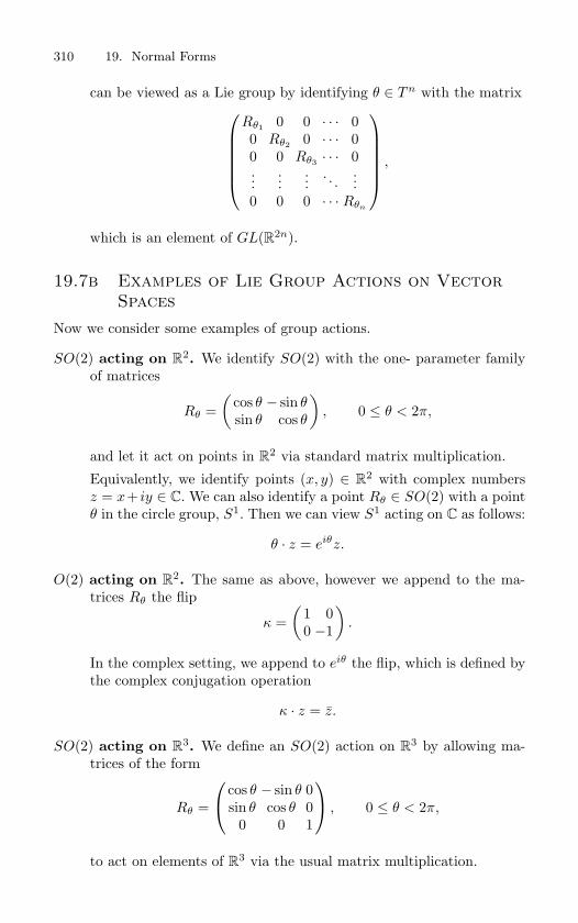
310 19. Normal Forms
can be viewed as a Lie group by identifying θ ∈ Tn with the matrix
Rθ1 0 0 · · · 00 Rθ2 0 · · · 00 0 Rθ3 · · · 0...
......
. . ....
0 0 0 · · · Rθn
,
which is an element of GL(R2n).
19.7b Examples of Lie Group Actions on VectorSpaces
Now we consider some examples of group actions.
SO(2) acting on R2. We identify SO(2) with the one- parameter family
of matrices
Rθ =(
cos θ − sin θsin θ cos θ
), 0 ≤ θ < 2π,
and let it act on points in R2 via standard matrix multiplication.
Equivalently, we identify points (x, y) ∈ R2 with complex numbers
z = x+ iy ∈ C. We can also identify a point Rθ ∈ SO(2) with a pointθ in the circle group, S1. Then we can view S1 acting on C as follows:
θ · z = eiθz.
O(2) acting on R2. The same as above, however we append to the ma-
trices Rθ the flip
κ =(
1 00 −1
).
In the complex setting, we append to eiθ the flip, which is defined bythe complex conjugation operation
κ · z = z.
SO(2) acting on R3. We define an SO(2) action on R
3 by allowing ma-trices of the form
Rθ =
cos θ − sin θ 0
sin θ cos θ 00 0 1
, 0 ≤ θ < 2π,
to act on elements of R3 via the usual matrix multiplication.
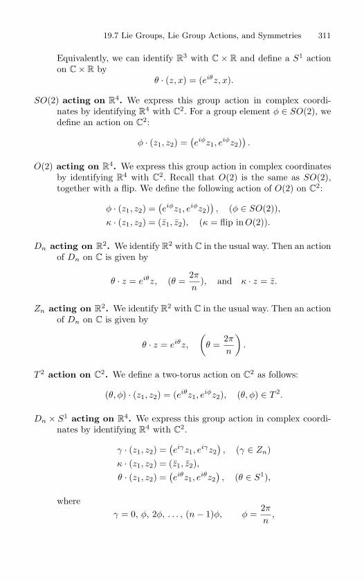
19.7 Lie Groups, Lie Group Actions, and Symmetries 311
Equivalently, we can identify R3 with C × R and define a S1 action
on C× R byθ · (z, x) = (eiθz, x).
SO(2) acting on R4. We express this group action in complex coordi-
nates by identifying R4 with C
2. For a group element φ ∈ SO(2), wedefine an action on C
2:
φ · (z1, z2) =(eiφz1, e
iφz2)).
O(2) acting on R4. We express this group action in complex coordinates
by identifying R4 with C
2. Recall that O(2) is the same as SO(2),together with a flip. We define the following action of O(2) on C
2:
φ · (z1, z2) =(eiφz1, e
iφz2)), (φ ∈ SO(2)),
κ · (z1, z2) = (z1, z2), (κ = flip inO(2)).
Dn acting on R2. We identify R
2 with C in the usual way. Then an actionof Dn on C is given by
θ · z = eiθz, (θ =2π
n), and κ · z = z.
Zn acting on R2. We identify R
2 with C in the usual way. Then an actionof Dn on C is given by
θ · z = eiθz,
(θ =
2π
n
).
T 2 action on C2. We define a two-torus action on C
2 as follows:
(θ, φ) · (z1, z2) = (eiθz1, eiφz2), (θ, φ) ∈ T 2.
Dn × S1 acting on R4. We express this group action in complex coordi-
nates by identifying R4 with C
2.
γ · (z1, z2) =(eiγz1, e
iγz2), (γ ∈ Zn)
κ · (z1, z2) = (z1, z2),θ · (z1, z2) =
(eiθz1, e
iθz2), (θ ∈ S1),
whereγ = 0, φ, 2φ, . . . , (n− 1)φ, φ =
2π
n,
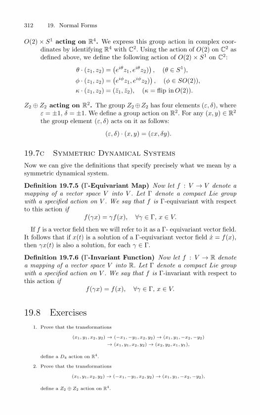
312 19. Normal Forms
O(2)× S1 acting on R4. We express this group action in complex coor-
dinates by identifying R4 with C
2. Using the action of O(2) on C2 as
defined above, we define the following action of O(2)× S1 on C2:
θ · (z1, z2) =(eiθz1, e
iθz2)), (θ ∈ S1),
φ · (z1, z2) =(eiφz1, e
iφz2)), (φ ∈ SO(2)),
κ · (z1, z2) = (z1, z2), (κ = flip inO(2)).
Z2 ⊕ Z2 acting on R2. The group Z2⊕Z2 has four elements (ε, δ), where
ε = ±1, δ = ±1. We define a group action on R2. For any (x, y) ∈ R
2
the group element (ε, δ) acts on it as follows:
(ε, δ) · (x, y) = (εx, δy).
19.7c Symmetric Dynamical SystemsNow we can give the definitions that specify precisely what we mean by asymmetric dynamical system.
Definition 19.7.5 (Γ-Equivariant Map) Now let f : V → V denote a
mapping of a vector space V into V . Let Γ denote a compact Lie group
with a specified action on V . We say that f is Γ-equivariant with respectto this action if
f(γx) = γf(x), ∀γ ∈ Γ, x ∈ V.
If f is a vector field then we will refer to it as a Γ- equivariant vector field.It follows that if x(t) is a solution of a Γ-equivariant vector field x = f(x),then γx(t) is also a solution, for each γ ∈ Γ.
Definition 19.7.6 (Γ-Invariant Function) Now let f : V → R denote
a mapping of a vector space V into R. Let Γ denote a compact Lie group
with a specified action on V . We say that f is Γ-invariant with respect tothis action if
f(γx) = f(x), ∀γ ∈ Γ, x ∈ V.
19.8 Exercises1. Prove that the transformations
(x1, y1, x2, y2) → (−x1, −y1, x2, y2) → (x1, y1, −x2, −y2)
→ (x1, y1, x2, y2) → (x2, y2, x1, y1),
define a D4 action on R4.
2. Prove that the transformations
(x1, y1, x2, y2) → (−x1, −y1, x2, y2) → (x1, y1, −x2, −y2),
define a Z2 ⊕ Z2 action on R4.
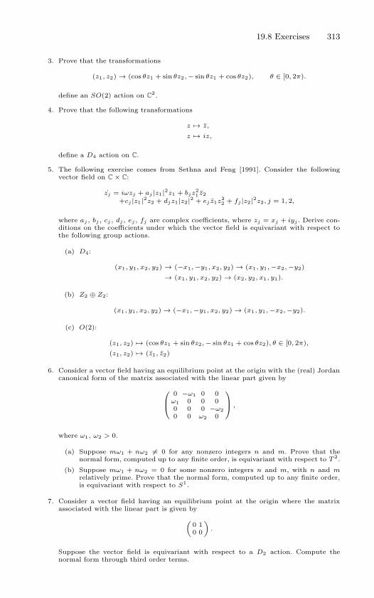
19.8 Exercises 313
3. Prove that the transformations
(z1, z2) → (cos θz1 + sin θz2, − sin θz1 + cos θz2), θ ∈ [0, 2π).
define an SO(2) action on C2.
4. Prove that the following transformations
z → z,
z → iz,
define a D4 action on C.
5. The following exercise comes from Sethna and Feng [1991]. Consider the followingvector field on C × C:
zj = iωzj + aj |z1|2z1 + bjz21 z2
+cj |z1|2z2 + djz1|z2|2 + ej z1z22 + fj |z2|2z2, j = 1, 2,
where aj , bj , cj , dj , ej , fj are complex coefficients, where zj = xj + iyj . Derive con-ditions on the coefficients under which the vector field is equivariant with respect tothe following group actions.
(a) D4:
(x1, y1, x2, y2) → (−x1, −y1, x2, y2) → (x1, y1, −x2, −y2)
→ (x1, y1, x2, y2) → (x2, y2, x1, y1).
(b) Z2 ⊕ Z2:
(x1, y1, x2, y2) → (−x1, −y1, x2, y2) → (x1, y1, −x2, −y2).
(c) O(2):
(z1, z2) → (cos θz1 + sin θz2, − sin θz1 + cos θz2), θ ∈ [0, 2π),
(z1, z2) → (z1, z2)
6. Consider a vector field having an equilibrium point at the origin with the (real) Jordancanonical form of the matrix associated with the linear part given by
0 −ω1 0 0ω1 0 0 00 0 0 −ω20 0 ω2 0
,
where ω1, ω2 > 0.
(a) Suppose mω1 + nω2 = 0 for any nonzero integers n and m. Prove that thenormal form, computed up to any finite order, is equivariant with respect to T 2.
(b) Suppose mω1 + nω2 = 0 for some nonzero integers n and m, with n and mrelatively prime. Prove that the normal form, computed up to any finite order,is equivariant with respect to S1.
7. Consider a vector field having an equilibrium point at the origin where the matrixassociated with the linear part is given by
(0 10 0
).
Suppose the vector field is equivariant with respect to a D2 action. Compute thenormal form through third order terms.
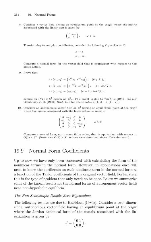
314 19. Normal Forms
8. Consider a vector field having an equilibrium point at the origin where the matrixassociated with the linear part is given by
(0 −ωω 0
), ω > 0.
Transforming to complex coordinates, consider the following D4 action on C:
z → z,
z → iz.
Compute a normal form for the vector field that is equivariant with respect to thisgroup action.
9. Prove that:
θ · (z1, z2) =(
eiθ
z1, eiθ
z2))
, (θ ∈ S1),
φ · (z1, z2) =(
e−iφ
z1, eiφ
z2))
, (φ ∈ SO(2)),
κ · (z1, z2) = (z2, z1), (κ = flip in O(2)),
defines an O(2) × S1 action on C2. (This result is due to van Gils [1984], see also
Golubitsky et al. [1988]. Hint: Use the coordinates z2(1, i) + z1(1, −i).)
10. Consider an autonomous vector field on R4 having an equilibrium point at the origin
where the matrix associated with the linearization is given by
0 −ω1 0 0ω1 0 0 00 0 0 −ω20 0 ω2 0
, ω > 0.
Compute a normal form, up to some finite order, that is equivariant with respect toO(2) × S1. (Note: two O(2) × S1 actions were described above. Consider each.)
19.9 Normal Form Coefficients
Up to now we have only been concerned with calculating the form of thenonlinear terms in the normal form. However, in applications once willneed to know the coefficents on each nonlinear term in the normal form asa function of the Taylor coefficients of the original vector field. Fortunately,this is the type of problem that only needs to be once. Below we summarizesome of the known results for the normal forms of autonomous vector fieldsnear non-hyperbolic equilibria.
The Non-Semisimple Double Zero Eigenvalue:
The following results are due to Knobloch [1986a]. Consider a two- dimen-sional autonomous vector field having an equilibrium point at the originwhere the Jordan canonical form of the matrix associated with the lin-earization is given by
J =(
0 10 0
).
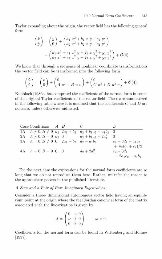
19.9 Normal Form Coefficients 315
Taylor expanding about the origin, the vector field has the following generalform (
xy
)=
(y0
)+
(a1 x2 + b1 x y + c1 y2
a2 x2 + b2 x y + c2 y2
)
+(
d1 x3 + e1 x2 y + f1 x y2 + g1 y3
d2 x3 + e2 x2 y + f2 x y2 + g2 y3
)+O(4)
We know that through a sequence of nonlinear coordinate transformationsthe vector field can be transformed into the following form(
uv
)=
(v0
)+
(0A u2 + B u v
)+
(0C u3 + D u2 v
)+O(4).
Knobloch [1986a] has computed the coefficients of the normal form in termsof the original Taylor coefficients of the vector field. These are summarizedin the following table where it is assumed that the coefficients C and D arenonzero, unless otherwise indicated.
Case Conditions A B C D1A A = 0, B = 0 a2 2a1 + b2 d2 + b1a2 − a1b2 02A A = 0, B = 0 a2 0 d2 + b1a2 + 2a2
1 03A A = 0, B = 0 0 2a1 + b2 d2 − a1b2 e2 + 3d1 − a1c2
+ b2(b1 + c2)/24A A = 0, B = 0 0 0 d2 + 2a2
1 e2 + 3d1− 2a1c2 − a1b1
For the next case the expressions for the normal form coefficients are solong that we do not reproduce them here. Rather, we refer the reader tothe appropriate papers in the published literature.
A Zero and a Pair of Pure Imaginary Eigenvalues:
Consider a three- dimensional autonomous vector field having an equilib-rium point at the origin where the real Jordan canonical form of the matrixassociated with the linearization is given by
J =
0 −ω 0
ω 0 00 0 0
, ω > 0.
Coefficients for the normal form can be found in Wittenberg and Holmes[1997].
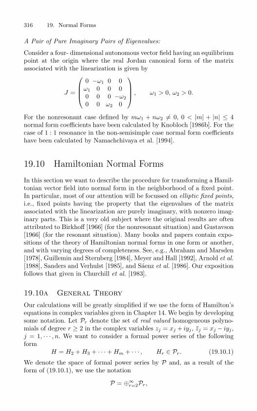
316 19. Normal Forms
A Pair of Pure Imaginary Pairs of Eigenvalues:
Consider a four- dimensional autonomous vector field having an equilibriumpoint at the origin where the real Jordan canonical form of the matrixassociated with the linearization is given by
J =
0 −ω1 0 0ω1 0 0 00 0 0 −ω20 0 ω2 0
, ω1 > 0, ω2 > 0.
For the nonresonant case defined by mω1 + nω2 = 0, 0 < |m| + |n| ≤ 4normal form coefficients have been calculated by Knobloch [1986b]. For thecase of 1 : 1 resonance in the non-semisimple case normal form coefficientshave been calculated by Namachchivaya et al. [1994].
19.10 Hamiltonian Normal Forms
In this section we want to describe the procedure for transforming a Hamil-tonian vector field into normal form in the neighborhood of a fixed point.In particular, most of our attention will be focussed on elliptic fixed points,i.e., fixed points having the property that the eigenvalues of the matrixassociated with the linearization are purely imaginary, with nonzero imag-inary parts. This is a very old subject where the original results are oftenattributed to Birkhoff [1966] (for the nonresonant situation) and Gustavson[1966] (for the resonant situation). Many books and papers contain expo-sitions of the theory of Hamiltonian normal forms in one form or another,and with varying degrees of completeness. See, e.g., Abraham and Marsden[1978], Guillemin and Sternberg [1984], Meyer and Hall [1992], Arnold et al.
[1988], Sanders and Verhulst [1985], and Saenz et al. [1986]. Our expositionfollows that given in Churchill et al. [1983].
19.10a General TheoryOur calculations will be greatly simplified if we use the form of Hamilton’sequations in complex variables given in Chapter 14. We begin by developingsome notation. Let Pr denote the set of real valued homogeneous polyno-mials of degree r ≥ 2 in the complex variables zj = xj + iyj , zj = xj − iyj ,j = 1, · · · , n. We want to consider a formal power series of the followingform
H = H2 + H3 + · · ·+ Hm + · · · , Hr ∈ Pr. (19.10.1)
We denote the space of formal power series by P and, as a result of theform of (19.10.1), we use the notation
P = ⊕∞r=2Pr,
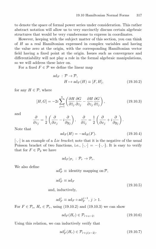
19.10 Hamiltonian Normal Forms 317
to denote the space of formal power series under consideration. This ratherabstract notation will allow us to very succinctly discuss certain algebraicstructures that would be very cumbersome to express in coordinates.
However, keeping with the subject matter of this section, you can thinkof H as a real Hamiltonian expressed in complex variables and havingthe value zero at the origin, with the corresponding Hamiltonian vectorfield having a fixed point at the origin. Issues such as convergence anddifferentiability will not play a role in the formal algebraic manipulations,so we will address these later on.
For a fixed F ∈ P we define the linear map
adF : P → P,
H → adF (H) ≡ [F, H], (19.10.2)
for any H ∈ P, where
[H,G] = −2in∑
j=1
(∂H
∂zj
∂G
∂zj− ∂H
∂zj
∂G
∂zj
), (19.10.3)
and∂
∂zj=
12
(∂
∂xj− i
∂
∂yj
),
∂
∂zj=
12
(∂
∂xj+ i
∂
∂yj
).
Note thatadF (H) = −adH(F ). (19.10.4)
[·, ·] is an example of a Lie bracket; note that it is the negative of the usualPoisson bracket of two functions, i.e., [·, ·] = −·, ·. It is easy to verifythat for F ∈ P2 we have
adF |Pr: Pr → Pr.
We also definead0
F ≡ identity mapping onP,
ad1F ≡ adF
and, inductively,
adjF ≡ adF adj−1
F , j > 1.
(19.10.5)
For F ∈ Ps, Hr ∈ Pr, using (19.10.2) and (19.10.3) we can show
adF (Hr) ∈ Pr+s−2. (19.10.6)
Using this relation, we can inductively verify that
adjF (Hr) ∈ Pr+j(s−2). (19.10.7)
318 19. Normal Forms
The exponential map will also play an important role for Hamiltonian nor-mal forms. For K ∈ Ps we define
exp(adK) : P → P
H →∞∑
j=0
1j!
adjK(H) ≡ exp (adK)(H)) . (19.10.8)
We now define what we mean by the term normal form of a Hamiltonian.
Definition 19.10.1 (Normal Form) An element H = ⊕∞r=2Hr ∈ P is
said to be in normal form through terms of order m ≥ 2 with respect toF ∈ P if adF (Hr) = 0 for 2 ≤ r ≤ m.
The following definition is important for the procedure of computing thenormal form.
Definition 19.10.2 (Splitting) F ∈ Pr is said to split P if for r ≥ 2 we
have
Pr = Nr ⊕Rr
where Nr = Ker (adF |Pr) and Rr = Im (adF |Pr
). When F splits P then
adF |Rr is an isomorphism and we let Γr : Rr → Rr denote the inverse.
The following is the main normal form theorem and provides an algo-rithm for transforming a Hamiltonian into normal form order-by-order.
Theorem 19.10.3 Let H = ⊕∞r=2Hr ∈ P be in normal form through terms
of order (m − 1) ≥ 2 with respect to H2, and assume that H2 splits P.
Let Hm = Hm + Hm, where Hm ∈ Nm and Hm ∈ Rm, and set Km =Γm
(Hm
). Then exp (adKm
) (H) is in normal form through terms of order
m with respect to H2, it agrees with H through terms of order m− 1, and
it has Hm as the mth term.
Proof: From (19.10.8) we have
exp (adKm) (H) =
∞∑j=0
1j!
adjKm
(H)
= H + adKm(H) + terms inPj , j ≥ 2m− 2
= H2 + H3 + · · ·+ Hm−1 + Hm + adKm(H2)
+ terms inPj , j ≥ m + 1 , (19.10.9)
which one easily sees agrees with H through terms of order m− 1.
19.10 Hamiltonian Normal Forms 319
Next we want to show that (19.10.9) is in normal form through order mwith respect to H2. For this to be true, by definition 19.10.1 we must have
adH2 (Hm + adKm(H2)) = 0.
This can be verified through the following simple calculations:
adH2 (Hm + adKm(H2)) = adH2(Hm) + adH2 (adKm
(H2))= adH2(Hm)− adH2 (adH2(Km))= adH2 (Hm − adH2(Km))
= adH2
(Hm − adH2(ad−1
H2(Hm)
)= adH2(Hm − Hm)= adH2(Hm) = 0, (19.10.10)
since Hm ∈ Nm. This calculation also reveals that the order m term in thenormal form is Hm. More precisely, the order m term of (19.10.9) is givenby
Hm + adKm(H2) = Hm − adH2(Km)= Hm − Hm = Hm. (19.10.11)
The theorem is now proved. The following results show how the normalization transformations are
related to symplectic or canonical transformations.
Proposition 19.10.4 Let H(z, z) =∑∞
j=2 Hj(z, z) converge in some
neighborhood U of the origin in R2n. Assume that H, considered as an
element of P, is in normal form with respect to H2 through terms of order
(m−1) ≥ 2. Denote Hm = Hm + Hm, where Hm ∈ Nm and Hm ∈ Rm, set
Km = Γm(Hm), and let φt denote the flow generated by the Hamiltonian
vector field z = −2i∂Km
∂z . Then
1. There is a neighborhood V ⊂ U of the origin such that φt is defined
in V for all |t| ≤ 2; and
2. exp(adKm)(H) = H φ1.
We remark that coordinate transformations generated by the time-oneflow map of the solutions of Hamilton’s equations are often referred to asLie transforms.
Proof:
1. The origin is an equilibrium point, hence the flow exists at this pointfor all t. Since flows have open domains, there is an open set contain-ing the origin such that the flow is defined for |t| ≤ 2.
320 19. Normal Forms
2. Let F (t) = H φt. Taylor expanding F (t) about t = 0 gives
F (t) = F (0)+F ′(0)t+12!
F ′′(0)t2 + · · ·+ 1n!
F (n)tn + · · · . (19.10.12)
Now we want to evaluate the Taylor coefficients. Recall that
adKm(H) = [Km, H] = −Km, H = H,Km ,
hence, from the formula for the time evolution of a function underthe flow generated by a Hamiltonian vector field (see Chapter 14),we have
F ′(t) =d
dt(H φt) = adKm
(H) φt.
Repeatedly differentiating this expression, we find
F ′′(t) = ad2Km
(H) φt
F ′′′(t) = ad3Km
(H) φt
...F (n)(t) = adn
Km(H) φt
...
and substituting these expressions into (19.10.12) gives
F (1) = H φ1 = 1l + adKm(H)
+12!
ad2Km
(H) + · · ·+ 1n!
adnKm
(H) + · · ·
=∞∑
j=0
1j!
adjKm
(H) ≡ exp (adKm) (H),(19.10.13)
which proves the result.
Corollary 19.10.5 exp(adKm) is a symplectic transformation.
Proof: This follows immediately from Theorem 14.3.6 in Chapter 14 sinceexp(adKm
)(H) = H φ1, and φ1 is the time-one map obtained from aHamiltonian flow.
19.10 Hamiltonian Normal Forms 321
An Example Calculation: Normalization Through Terms ofO(3)
We will now illustrate the use of Theorem 19.10.3 by beginning with aHamiltonian of the form
H = H2 + H3 + H4 + · · ·+ Hm + · · · ,and normalizing it through terms of O(3). From Theorem 19.10.3 we have
exp (adK3) (H) = H + adK3(H) +12ad2
K3(H)
+ terms inPj , j ≥ 5
= H2 + H3 + H3 + adK3(H2)
+ H4 + adK3(H3) +12ad2
K3(H2)︸ ︷︷ ︸
O(4) terms
+O(5)
(19.10.14)
NowadH2(K3) = adH2
(ad−1
H2(H3)
)= H3 = −adK3(H2),
from which it also follows that
ad2K3
(H2) = −adK3
(H3
),
Using these to relations, (19.10.14) can be written as
exp (adK3(H)) = H2 + H3 + H4 + adK3(H3)−12adK3(H3)︸ ︷︷ ︸
O(4) terms
+O(5).
(19.10.15)This equation can be further simplified. Note that
adK3(H3)−12adK3(H3) = adK3(H3)− adK3(H3)
+12adK3(H3)
= adK3(H3 − H3) +12adK3(H3)
= adK3(H3) +12adK3(H3) (19.10.16)
Substituting this expression into (19.10.15) gives
exp (adK3(H)) = H2 + H3 + H4 + adK3(H3) +12adK3(H3)︸ ︷︷ ︸
O(4) terms
+O(5).
(19.10.17)
322 19. Normal Forms
By Theorem 19.10.3, (19.10.17) is in normal form with respect to H2through terms of order 3.
We make several remarks concerning this computation.
1. Normalizing the O(3) terms modified the O(4) terms, but did not
modify the O(2) terms.
2. Note that in deriving explicit expressions for the normal form we willneed to compute Km. We will address this issue in a more explicitcontext in the next subsection.
3. How might one use a partially normalized Hamiltonian such as(19.10.17)? One situation is if the normalized part possesses somespecial solutions or structure, e.g. it possesses periodic orbits it isintegrable. In that case, by appropriate scaling, one may be able toconsider the unnormalized part of the Hamiltonian, or “tail” as aperturbation to the normalized part. The advantage of this lies inthe fact that there are a great deal of techniques for studying per-turbations of periodic orbits and completely integrable Hamiltoniansystems.
19.10b Normal Forms Near Elliptic Fixed Points:The Semisimple Case
Now we specialize to the case that will be our primary interest. Henceforthwe will assume that
H2(z, z) =n∑
j=1
ωj
2|zj |2 ∈ P2. (19.10.18)
This is the Hamiltonian corresponding to a linear Hamiltonian vector fieldhaving an elliptic fixed point at the origin, i.e., the eigenvalues of the matrixassociated with the linear vector field are ±iω1, · · · ,±iωn, ωi = 0. Thisform assumes that the linearization is semisimple, i.e, it’s complexificationis diagonalizable, which is true if the ωi, i = 1, · · · , n, are distinct.
Definition 19.10.6 An elliptic fixed point is said to be resonant if there
exists a nonzero integer n-vector, i.e., k ∈ ZZn − 0, such that
〈k, ω〉 ≡n∑
i=1
kiωi = 0. (19.10.19)
The order of the resonance is defined to be
|k| ≡n∑
i=1
|ki|.
19.10 Hamiltonian Normal Forms 323
For fixed ω, the number of independent integer vectors that solve (19.10.19)
is referred to as the multiplicity of the resonance. If (19.10.19) has no
integer solutions, then the elliptic fixed point is said to be nonresonant.
The following abbreviated notation will be used throughout the remain-der of this section
zkzl ≡ zk11 · · · zkn
n zl11 · · · zln
n , ki, li ≥ 0, i = 1, · · · , n, (19.10.20)
and
〈k − l, ω〉 ≡n∑
j=1
(kj − lj)ωj . (19.10.21)
Next we give a proposition that shows why the method of normalizationis often referred to as averaging, since we will show that the terms thatcannot be removed by the normal form transformation are averages overtrajectories of the Hamiltonian vector field corresponding to H2(z, z) =∑n
j=1ωj
2 |zj |2.
Proposition 19.10.7 Let ρt denote the flow generated by the Hamiltonian
vector field z = −2i∂H2∂z . Then
Hm(z, z) = limT→∞
1T
∫ T
0(Hm ρt) (z, z)dt.
Proof: By definition 19.10.1 we have adH2(Hm) = 0, hence
d
dt
(Hm ρt
)= adH2(Hm) ρt = 0, (19.10.22)
which implies that Hm is constant on trajectories generated by the Hamil-tonian vector field corresponding to H2. Recall also that
d
dt(Km ρt) = adH2
(Γm(Hm)
) ρt = Hm ρt. (19.10.23)
Now we consider the following calculation
limT→∞
1T
∫ T
0(Hm ρt) (z, z)dt
= limT→∞
1T
∫ T
0
(Hm ρt
)(z, z)dt + lim
T→∞
1T
∫ T
0
(Hm ρt
)(z, z)dt
(19.10.24)
From (19.10.22), the first term in (19.10.24) is given by
limT→∞
1T
∫ T
0
(Hm ρt
)(z, z)dt = Hm(z, z). (19.10.25)
324 19. Normal Forms
It remains to show that the second expression in (19.10.24) is zero, i.e.,
limT→∞
1T
∫ T
0
(Hm ρt
)(z, z)dt = 0. (19.10.26)
From (19.10.23), we have (using φ0 = 1l)
1T
∫ T
0
(Hm ρt
)(z, z)dt =
1T
(Km ρT −Km) . (19.10.27)
Equation (19.10.26) will follow if we show that show that Km ρT isbounded for all T . But this is true since the components of ρt(z, z) aregiven by zj(t) = zje
iωjt, j = 1, . . . , n.
Real Hamiltonians as Functions of Complex Variables: SomeProperties
For explicit calculations we will need more concrete notation. We will ex-press our Hamiltonians in the form of a power series
H(z, z) =∞∑
|k|+|l|=2
cklzkzl,
with|k|+ |l| ≡ k1 + · · ·+ kn + l1 + · · ·+ ln, ki, li ≥ 0.
For real Hamiltonians several relations between the coefficients of the powerseries hold. Moreover, certain algebraic simplifications of terms are possible.We now want to catalog these for future reference.
ckl = clk This can be seen as follows. For real Hamiltonians we have
H(z, z) = H(z, z).
The Hamiltonians that we are now considering have the followingrepresentation
H(z, z) =∞∑
|k|+|l|=2
cklzkzl, (19.10.28)
and, hence, their complex conjugates are given by
H(z, z) =∞∑
|k|+|l|=2
cklzkzl =∞∑
|k|+|l|=2
cklzkzl. (19.10.29)
Reality implies that (19.10.28) and (19.10.29) are equal. Equating thecoefficients of each term in (19.10.28) and (19.10.29) gives
ckl = clk. (19.10.30)
19.10 Hamiltonian Normal Forms 325
If k = l then clk is real This is an immediate consequence of (19.10.30).
Algebraic Simplification, I The following relation will be useful lateron in simplifying normal forms that we compute. Suppose that theHamiltonian has two terms of the same order having the followingform
cklzkzl + clkzlzk,
whereckl ≡ a + ib.
Then this term can be simplified as follows
cklzkzl + clkzlzk,
= cklzkzl + cklz
lzk, using (19.10.30),
= cklzkzl + cklzkzl,
= (a + ib)(Re zkzl + iIm zkzl)+(a− ib)(Re zkzl − iIm zkzl),
= 2aRe zkzl − 2bImzkzl.
(19.10.31)
Algebraic Simplification, II In the case where kj = lj , for some 1 ≤j ≤ n with at least one of these two exponents nonzero, this last termcan be simplified even further:
2aRe zkzl − 2bImzkzl
= Re[2aRe zkzl + i2aIm zkzl + i2bRe zkzl − 2bIm zkzl
]= Re
[2(a + ib)(Rezkzl + iIm zkzl)
]= 2Re
[(a + ib)zkzl
].
(19.10.32)
Now denotea + ib = c, c = |c|ei arg c.
Suppose that in the term
zk11 · · · zkn
n zl11 · · · zln
n
there exists exponents such that kj = lj , for some 1 ≤ j ≤ n, with atleast one of the two nonzero.
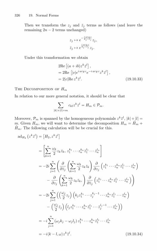
326 19. Normal Forms
Then we transform the zj and zj terms as follows (and leave theremaining 2n− 2 terms unchanged)
zj → e− i arg c
kj−lj zj ,
zj → ei arg ckj−lj zj .
Under this transformation we obtain
2Re[(a + ib)zkzl
],
= 2Re[|c|ei arg ce−i arg czkzl
],
= 2|c|Re zkzl. (19.10.33)
The Decomposition of Hm
In relation to our more general notation, it should be clear that∑|k|+|l|=m
cklzkzl = Hm ∈ Pm.
Moreover, Pm is spanned by the homogeneous polynomials zkzl, |k|+ |l| =m. Given Hm, we will want to determine the decomposition Hm = Hm +Hm. The following calculation will be be crucial for this.
adH2
(zkzl
)=
[H2, z
kzl]
=
[n∑
k=1
ωk
2zkzk, zk1
1 · · · zknn zl1
1 · · · zlnn
]
= −2i
n∑j=1
(∂
∂zj
(n∑
k=1
ωk
2zkzk
)∂
∂zj
(zk11 · · · zkn
n zl11 · · · zln
n
)
− ∂
∂zj
(n∑
k=1
ωk
2zkzk,
)∂
∂zj
(zk11 · · · zkn
n zl11 · · · zln
n
))
= −2in∑
j=1
((ωj
2zj
)(kjz
k11 · · · zkj−1
j · · · zknn zl1
1 · · · zlnn
)−
(ωj
2zj
)(ljz
k11 · · · zkn
n zl11 · · · z
lj−1j · · · zln
n
))
= −in∑
j=1
(ωjkj − ωj lj) zk11 · · · zkn
n zl11 · · · zln
n
= −i〈k − l, ω〉zkzl. (19.10.34)
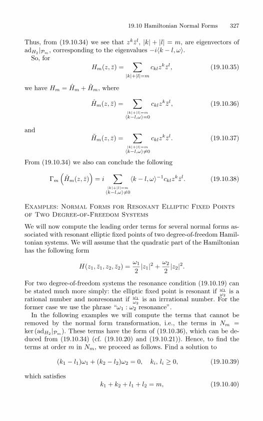
19.10 Hamiltonian Normal Forms 327
Thus, from (19.10.34) we see that zkzl, |k| + |l| = m, are eigenvectors ofadH2 |Pm
, corresponding to the eigenvalues −i〈k − l, ω〉.So, for
Hm(z, z) =∑
|k|+|l|=m
cklzkzl, (19.10.35)
we have Hm = Hm + Hm, where
Hm(z, z) =∑
|k|+|l|=m
〈k−l,ω〉=0
cklzkzl, (19.10.36)
andHm(z, z) =
∑|k|+|l|=m
〈k−l,ω〉=0
cklzkzl. (19.10.37)
From (19.10.34) we also can conclude the following
Γm
(Hm(z, z)
)= i
∑|k|+|l|=m
〈k−l,ω〉=0
〈k − l, ω〉−1cklzkzl. (19.10.38)
Examples: Normal Forms for Resonant Elliptic Fixed Pointsof Two Degree-of-Freedom Systems
We will now compute the leading order terms for several normal forms as-sociated with resonant elliptic fixed points of two degree-of-freedom Hamil-tonian systems. We will assume that the quadratic part of the Hamiltonianhas the following form
H(z1, z1, z2, z2) =ω1
2|z1|2 +
ω2
2|z2|2.
For two degree-of-freedom systems the resonance condition (19.10.19) canbe stated much more simply: the elliptic fixed point is resonant if ω1
ω2is a
rational number and nonresonant if ω1ω2
is an irrrational number. For theformer case we use the phrase “ω1 : ω2 resonance”.
In the following examples we will compute the terms that cannot beremoved by the normal form transformation, i.e., the terms in Nm =ker (adH2 |Pm
). These terms have the form of (19.10.36), which can be de-duced from (19.10.34) (cf. (19.10.20) and (19.10.21)). Hence, to find theterms at order m in Nm, we proceed as follows. Find a solution to
(k1 − l1)ω1 + (k2 − l2)ω2 = 0, ki, li ≥ 0, (19.10.39)
which satisfiesk1 + k2 + l1 + l2 = m, (19.10.40)
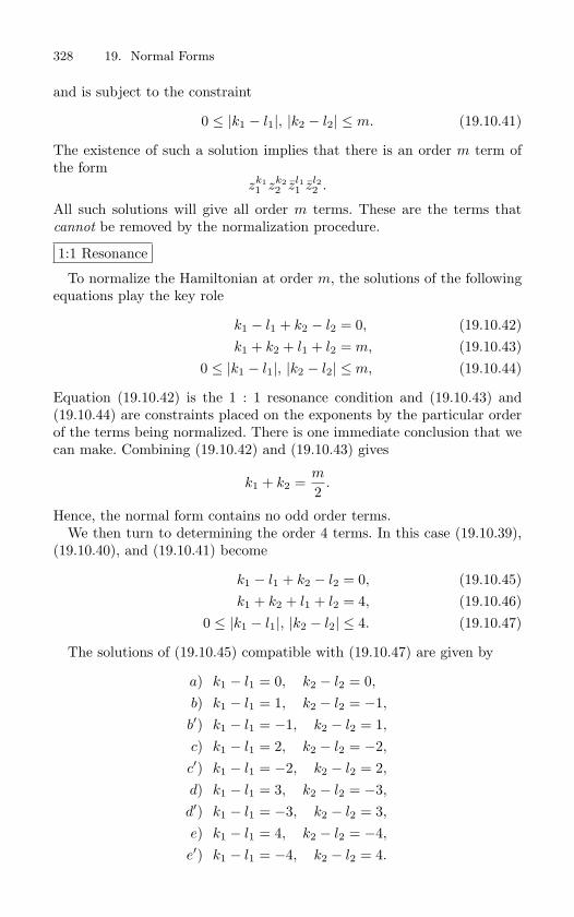
328 19. Normal Forms
and is subject to the constraint
0 ≤ |k1 − l1|, |k2 − l2| ≤ m. (19.10.41)
The existence of such a solution implies that there is an order m term ofthe form
zk11 zk2
2 zl11 zl2
2 .
All such solutions will give all order m terms. These are the terms thatcannot be removed by the normalization procedure.
1:1 Resonance
To normalize the Hamiltonian at order m, the solutions of the followingequations play the key role
k1 − l1 + k2 − l2 = 0, (19.10.42)k1 + k2 + l1 + l2 = m, (19.10.43)
0 ≤ |k1 − l1|, |k2 − l2| ≤m, (19.10.44)
Equation (19.10.42) is the 1 : 1 resonance condition and (19.10.43) and(19.10.44) are constraints placed on the exponents by the particular orderof the terms being normalized. There is one immediate conclusion that wecan make. Combining (19.10.42) and (19.10.43) gives
k1 + k2 =m
2.
Hence, the normal form contains no odd order terms.We then turn to determining the order 4 terms. In this case (19.10.39),
(19.10.40), and (19.10.41) become
k1 − l1 + k2 − l2 = 0, (19.10.45)k1 + k2 + l1 + l2 = 4, (19.10.46)
0 ≤ |k1 − l1|, |k2 − l2| ≤ 4. (19.10.47)
The solutions of (19.10.45) compatible with (19.10.47) are given by
a) k1 − l1 = 0, k2 − l2 = 0,
b) k1 − l1 = 1, k2 − l2 = −1,
b′) k1 − l1 = −1, k2 − l2 = 1,
c) k1 − l1 = 2, k2 − l2 = −2,
c′) k1 − l1 = −2, k2 − l2 = 2,
d) k1 − l1 = 3, k2 − l2 = −3,
d′) k1 − l1 = −3, k2 − l2 = 3,
e) k1 − l1 = 4, k2 − l2 = −4,
e′) k1 − l1 = −4, k2 − l2 = 4.
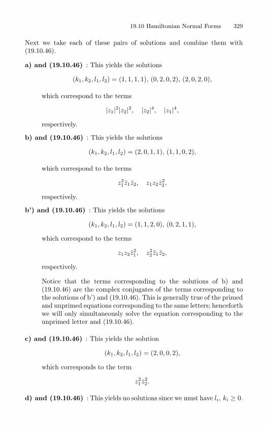
19.10 Hamiltonian Normal Forms 329
Next we take each of these pairs of solutions and combine them with(19.10.46).
a) and (19.10.46) : This yields the solutions
(k1, k2, l1, l2) = (1, 1, 1, 1), (0, 2, 0, 2), (2, 0, 2, 0),
which correspond to the terms
|z1|2|z2|2, |z2|4, |z1|4,
respectively.
b) and (19.10.46) : This yields the solutions
(k1, k2, l1, l2) = (2, 0, 1, 1), (1, 1, 0, 2),
which correspond to the terms
z21 z1z2, z1z2z
22 ,
respectively.
b’) and (19.10.46) : This yields the solutions
(k1, k2, l1, l2) = (1, 1, 2, 0), (0, 2, 1, 1),
which correspond to the terms
z1z2z21 , z2
2 z1z2,
respectively.
Notice that the terms corresponding to the solutions of b) and(19.10.46) are the complex conjugates of the terms corresponding tothe solutions of b’) and (19.10.46). This is generally true of the primedand unprimed equations corresponding to the same letters; henceforthwe will only simultaneously solve the equation corresponding to theunprimed letter and (19.10.46).
c) and (19.10.46) : This yields the solution
(k1, k2, l1, l2) = (2, 0, 0, 2),
which corresponds to the term
z21 z2
2 .
d) and (19.10.46) : This yields no solutions since we must have li, ki ≥ 0.
330 19. Normal Forms
e) and (19.10.46) : This yields no solutions since we must have li, ki ≥ 0.
Hence, the normal form through order 4 terms has the form (where wehave remembered to put in the complex conjugate terms)
H(z1, z1, z2, z2) =12|z1|2 +
12|z2|2
+ c1111|z1|2|z2|2 + c0202|z2|4 + c2020|z1|4
+ 2ac2011z21 z1z2 + c1120z
21z1z2
+ c1102z1z2z22 + c0211z1z2z
22
+ c2002z21 z2
2 + c0220z21z2
2 +O(6), (19.10.48)
Using “algebraic simplification, II” given in Section 19.10b, the normalform can be written as
H(z1, z1, z2, z2) =12|z1|2 +
12|z2|2
+ c1111|z1|2|z2|2 + c0202|z2|4 + c2020|z1|4
+ 2aRez21 z1z2 − 2bImz2
1 z1z2
+ 2cRez1z2z22 − 2dImz1z2z
22
+ 2eRez21 z2
2 − 2fImz21z2
2 +O(6), (19.10.49)
where
c2011 = a + ib,
c1102 = c + id,
c2002 = e + if. (19.10.50)
Using “algebraic simplication, II” given in 19.10b, the normal form can bewritten as
H(z1, z1, z2, z2) = 12 |z1|2 + 1
2 |z2|2+c1111|z1|2|z2|2 + c0022|z2|4 + c2200|z1|4+2|c2011|Rez2
1 z1z2 + 2|c1102|Rez1z2z22 + 2|c2002|Rez2
1 z22
+O(6).
1:2 Resonance
Following the same procedure as in the 1 : 1 resonance case, we seeknonnegative integer solutions of the following equations
k1 − l1 + 2(k2 − l2) = 0, (19.10.51)k1 + k2 + l1 + l2 = 3, (19.10.52)
0 ≤ |k1 − l1|, |k2 − l2| ≤ 3. (19.10.53)
19.10 Hamiltonian Normal Forms 331
Solutions of (19.10.51) compatible with (19.10.53) are given by
a) k1 − l1 = 0, k2 − l2 = 0,
b) k1 − l1 = 2, k2 − l2 = −1,
b′) k1 − l1 = −2, k2 − l2 = 1,
We next seek simultaneous solutions of each of these pairs equations with(19.10.52).
a) and (19.10.52) : This yields no solutions since we must have li, ki ≥ 0.
b) and (19.10.52) : This yields the solution
(k1, k2, l1, l2) = (2, 0, 0, 1),
which corresponds to the term
z21 z2.
Solving b’) and (19.10.52) simultaneously gives rise to the complexconjugate of the term arising from the simultaneous solution of b)and (19.10.52).
Hence, the normal form through order 3 terms is given by (where wehave remembered to put in the complex conjugate terms)
H(z1, z1, z2, z2) =12|z1|2 + |z2|2 + c2001z
21 z2 + c0120z
21z2 +O(4), (19.10.54)
Using “algebraic simplification, I” given in section 19.10b, the normal formcan be written as
H(z1, z1, z2, z2) =12|z1|2 + |z2|2 +2aRez2
1 z2−2bImz21 z2 +O(4), (19.10.55)
wherec2001 = a + ib.
Using “algebraic simplification, II” given in section 19.10b, the normal formcan be written as
H(z1, z1, z2, z2) =12|z1|2 + |z2|2 + 2|c2001|Rez2
1 z2 +O(4), (19.10.56)
1:3 Resonance
Following the same procedure as in the previous two cases, we find thatthere are no third order terms. The fourth order terms can be obtainedthrough solution of the following equations
k1 − l1 + 3(k2 − l2) = 0, (19.10.57)k1 + k2 + l1 + l2 = 4, (19.10.58)
0 ≤ |k1 − l1|, |k2 − l2| ≤ 4. (19.10.59)
332 19. Normal Forms
Solutions of (19.10.57) compatible with (19.10.59) are given by
a) k1 − l1 = 0, k2 − l2 = 0,
b) k1 − l1 = 3, k2 − l2 = −1,
b′) k1 − l1 = −3, k2 − l2 = 1.
We next solve each of these pairs of equations simultaneously with(19.10.58).
a) and (19.10.52) : This yields the solutions
(k1, k2, l1, l2) = (0, 2, 0, 2), (2, 0, 2, 0), (1, 1, 1, 1),
which correspond to the terms
|z2|4, |z1|4, |z1|2|z2|2,
respectively.
b) and (19.10.52) : This yields the solutions
(k1, k2, l1, l2) = (3, 0, 0, 1),
which correspond to the terms
z31 z2.
Solution of b’) and (19.10.58) yields the complex conjugate of thisterm.
Hence, the normal form through order 4 terms is given by (where wehave remembered to put in the complex conjugate terms)
H(z1, z1, z2, z2) =12|z1|2 +
32|z2|2
+ c0202|z2|4 + c2020|z1|4 + c1111|z1|2|z2|2
+ c3001z31 z2 + c0130z
31z2 +O(5), (19.10.60)
Using “algebraic simplification, I” given in section 19.10b, the normal formcan be written as
H(z1, z1, z2, z2) =12|z1|2 +
32|z2|2
+ c0202|z2|4 + c2020|z1|4 + c1111|z1|2|z2|2
+ 2aRez31 z2 − 2bImz3
1 z2 +O(5), (19.10.61)
19.10 Hamiltonian Normal Forms 333
wherec3001 = a + ib.
Using “algebraic simplification, II” given in section 19.10b, the normal formcan be written as
H(z1, z1, z2, z2) =12|z1|2 +
32|z2|2
+ c0202|z2|4 + c2020|z1|4 + c1111|z1|2|z2|2
+ 2|c3001|Rez31 z2 +O(5). (19.10.62)
There is a large literature on the analysis of the dynamics near resonantelliptic fixed points in two degree-of-freedom Hamiltonian systems; see, e.g.,Arnold et al. [1988], Sanders and Verhulst [1985], Henrard [1970], Meyerand Hall [1992], and Golubitsky et al. [1995].
19.10c The Birkhoff and Gustavson Normal FormsWe now describe the Birkhoff normal form and the Gustavson normal form.These are normal forms in the neighborhood of an elliptic fixed point inthe nonresonant and resonant cases, respectively. We begin with some def-initions.
First we recall the form of the Hamiltonian in the neighborhood of anelliptic fixed point that we described earlier:
H(z, z) =12
n∑i=1
ωi|z1|2 + H3(z, z) + H4(z, z) + · · · . (19.10.63)
Near an elliptic equilibrium point symplectic polar coordinates provide auseful coordinate system. These are related to the complex coordinates by
zk ≡√
2ρkeiϕk , zk ≡√
2ρke−iϕk , k = 1, . . . , n.
However, one must be aware that singularities may arise as ρk → 0. Nextwe define the notion of Birkhoff normal form near an elliptic equilibriumpoint.
Definition 19.10.8 (Birkhoff Normal Form) The Hamiltonian
(19.10.63) is said to be in Birkhoff normal form of degree r if it is a poly-
nomial of degree r in zi, zi, which is actually a polynomial of degree[
r2
]in
the variables ρi = 12 |zi|2, where
[r2
]denotes the integer part of the number
r2 .
Example 19.10.1. Consider the two degree-of-freedom version of (19.10.63)
with terms through order 4. Then the Birkhoff normal form of degree 4 has the
form
H = ω1ρ1 + ω2ρ2 + aρ21 + bρ1ρ2 + cρ2
2.
End of Example 19.10.1
334 19. Normal Forms
Now we can state Birkhoff’s theorem (Birkhoff [1966]).
Theorem 19.10.9 (Birkhoff) Suppose the ωi in (19.10.63) satisfy no
resonance relations of order less than or equal to r. Then there exists a
symplectic change of coordinates defined in a neighborhood of the origin
such that in the new coordinates the Hamiltonian is reduced to Birkhoff
normal form of degree r up to terms of order r + 1, i.e.,
H = Hr(ρ) +O(|z|, |z|)r+1.
Proof: See Exercise 3. Next we consider the case where there are some resonances of order less
than or equal to r. In this case we first define what we mean by a resonant
normal form near an elliptic equilibrium point.
Definition 19.10.10 (Resonant Normal Form) Let K be a subgroup
of the lattice of integers ZZn. A resonant normal form of degree r under res-onances from K (or, a K resonant normal form of degree r) is a polynomial
of degree r in zi, zi which, when expressed in terms of polar coordinates,
depends only on the phases through the combinations k · ϕ, with k ∈ K.
Now we can state Gustavson’s theorem on resonant normal forms (Gus-tavson [1966]).
Theorem 19.10.11 (Gustavson) Suppose the ωi in (19.10.63) satisfy
no resonance relations of order less than or equal to r, except, possibly,
for relations k · ω = 0, k ∈ K. Then there exists a symplectic change of
coordinates defined in a neighborhood of the origin such that in the new
coordinates the Hamiltonian is reduced to a K resonant normal form of
degree r up to terms of order r + 1.
Proof: See Exercise 4.
19.10d The Lyapunov Subcenter Theorem andMoser’s Theorem
We now describe two classical results that describe the behavior near equi-librium points of Hamiltonian systems.
Consider an n degree-of-freedom Hamiltonian having the following form
H(x, y) = H2(x, y) + H3(x, y) + H4(x, y) + · · · , (19.10.64)
wherex ≡ (x1, . . . , xn) ∈ R
n, y ≡ (y1, . . . , yn) ∈ Rn,
andH2(x, y) =
ω1
2(x2
1 + y21) + · · ·+ ωn
2(x2
n + y2n), (19.10.65)
19.10 Hamiltonian Normal Forms 335
and Hr denotes a homogeneous polynomial of degree r in x and y. We mustfurther assume that H is analytic in a neighborhood of the origin, whichis an elliptic equilibrium point for the corresponding Hamiltonian vectorfield.
Theorem 19.10.12 (Lyapunov Subcenter Theorem) If for all s > 1the ratio ωs
ω1is not an integer, then there exists an invertible, analytic,
canonical transformation (x, y) → (ξ, η) which transforms the Hamiltonian
H(x, y) to the form
H(ξ, η) = Φ(ρ) +O(|ζ|2), (19.10.66)
where Φ is a function of the single variable ρ = ξ21 + η2
1, and ζ =(ξ2, . . . , ξn, η2, . . . , ηn).
Proof: See Siegel and Moser [1971] and Moser [1958]. From the form of the transformed Hamiltonian one sees immediately that
ζ = 0 is a two dimensional invariant manifold, with the dynamics on thismanifold given by
ξ1 = 2dΦdρ
(ρ)η1,
η1 = −2dΦdρ
(ρ)ξ1.
If one multiplies the first equation by ξ1, the second by η1, adds themtogether and uses the definition of ρ one sees immediately that ρ is aconstant of the motion on this two dimensional invariant manifold. Sinceρ = ξ2
1 + η21 , we see that this two dimensional invariant manifold is filled
with periodic orbits. Moreover, the form of the equations, restricted to
the periodic orbit ρ=constant, is that of a linear harmonic oscillator withfrequency dΦ
dρ (ρ).The Lyapunov subcenter theorem states that under the nonresonance
assumptions given by the theorem, the corresponding two dimensional in-variant subspace of the linearized Hamiltonian vector field filled with peri-odic orbits, all having frequency ω1, persists for the full nonlinear problem,however the frequencies may change slightly. (Keep in mind that this is alocal result valid in a neighborhood of the equilibrium point.) If the nonres-onance condition is violated then the result does not hold in the sense thata manifold of periodic solutions does not exist for the nonlinear Hamilto-nian vector field (Roels [1971a], [1971b]). Periodic orbits may persist fromthe linearized problem. However, analytic manifolds of such solutions donot exist. See Weinstein [1973], Moser [1976], [1978], and Ito [1989].
There is one other point to be made. As mentioned in the remarks atthe end of our discussion of normal forms, generically normal form trans-formations are divergent when taken to all orders. However, it may be that
336 19. Normal Forms
the transformation is convergent on a lower dimensional submanifold, as itis in the situation described by the Lyapunov subcenter theorem.
Moser [1958] has generalized the Lyapunov subcenter theorem to the casewhere there is exactly one pair of real eigenvalues, λ and −λ. We state histheorem.
Theorem 19.10.13 (Moser’s Theorem) Suppose H2 in the Hamilto-
nian (19.10.64) has the form
H2(x, y) = λx1y1 +ω2
2(x2
2 + y22) + · · ·+ ωn
2(x2
n + y2n). (19.10.67)
Then there exists an invertible, analytic, canonical transformation (x, y) →(ξ, η) which transforms the Hamiltonian H(x, y) to the form
H(ξ, η) = Φ(ρ) +O(|ζ|2), (19.10.68)
where Φ is a function of the single variable ρ = ξ1η1, and ζ =(ξ2, . . . , ξn, η2, . . . , ηn).
Proof: See Moser [1958]. From the form of the transformed Hamiltonian one sees immediately that
ζ = 0 is a two dimensional invariant manifold, with the dynamics on thismanifold given by
ξ1 =dΦdρ
(ρ)ξ1,
η1 = −dΦdρ
(ρ)η1.
If one multiplies the first equation by η1, the second by ξ1, adds themtogether and uses the definition of ρ one sees immediately that ρ is aconstant of the motion on this two dimensional invariant manifold, andthe trajectories are given by the hyperbolae defined by ρ=constant.
19.10e The KAM and Nekhoroshev Theorem’sNear an Elliptic Equilibrium Point
Suppose the ωi in (19.10.63) satisfy no resonance relations of order lessthan or equal to 4. Then, in a neighborhood of the origin, the Hamiltoniancan be transformed to Birkhoff normal form through degree 4:
H = H0(ρ) +O(5), (19.10.69)
where
H0(ρ) =n∑
i=1
ωiρi +12
n∑i,j=1
ai,jρiρj .
19.10 Hamiltonian Normal Forms 337
The Hamiltonian H0(ρ) defines a completely integrable Hamiltonian systemwhere the trajectories lie on the invariant tori ρ = constant. Now for ρsufficently small one could view the O(5) terms as a perturbation of H0(ρ).In this case it is natural to think of trying to apply the KAM theorem tosee if any of the invariant tori of H0(ρ) are preserved when the effect ofthe O(5) terms is considered. This can be done if H0(ρ) is appropriatelynondegenerate, which we describe in more detail.
As is typical in KAM type arguments, we need a nondegeneracy assump-tion on the unperturbed Hamiltonian. The Hamiltonian H0(ρ) is said tobe nondegenerate if
det(
∂2H0
∂ρ2
) = 0,
and isoenergetically nondegenerate if
det
∂2H0∂ρ2
∂H0∂ρ
∂H0∂ρ 0
= 0.
We now have the following theorem due to Arnold [1963].
Theorem 19.10.14 (Arnold) For H0(ρ) either nondegenerate or isoen-
ergetically nondegnerate, in a sufficently small neighborhood of the origin
there exists invariant tori for H0(ρ) + O(5) having freqencies close to the
linearized frequencies ωi.
Proof: See Arnold [1963]. As one might suspect, there is also a version of Nekhoroshev’s theorem
that is valid in the neighborhood of an elliptic equilbrium point, the ωi in(19.10.63) satisfy no resonance relations of order less than or equal to 4. Inaddition, we assume that the matrix A ≡ (aij) is sign definite, say positive(if not, then multiply the Hamiltonian by −1), with spectrum boundedfrom below by m > 0 and bounded from above by M > 0.
Theorem 19.10.15 (Lochak) Consider a trajectory (z(t), z(t)) of the
Hamiltonian vector field generated by the Hamiltonian (19.10.69), writ-
ten in complex coordinates (z, z). There is a constant ν > 0 such that if
(z(0), z(0)) is small enough and satisfies
|zj(0)| ≥ ν ‖ z(0) ‖2+ 1n+2 , j = 1, . . . , n,
where ‖ · ‖ is the Euclidean norm, then one has
‖ zj(t)− z(0) ‖≤ ν
2‖ z(0) ‖2+ 1
n+2 , j = 1, . . . , n,
provided that t satisfies
|t| ≤ T exp(‖ z(0) ‖− 1
n+2
),
338 19. Normal Forms
where T is some strictly positive constant.
Proof: See Lochak [1992]. Polar coordinates are the natural “action-angle” coordinates in the neigh-
borhood of an elliptic equilibrium point. However, using polar coordinatescan present difficulties when studying trajectories in a neighborhood of anequilibrium point. The reason for this is that a singularity develops whena component of the radius vector goes to zero. This problem has beenovercome in the recent work of Niederman [1998] and Fasso et al. [1998].
19.10f Hamiltonian Normal Forms and SymmetriesIn this subsection we will deal with the situation where the Hamiltonianwhich we are transforming to normal form has a symmetry. The mainresult is that the normal form, through any finite order which we wish tocalculate, will have the same symmetry. All the results in this subsectionare from Churchill et al. [1983].
We recall our earlier notation. Let
P = ⊕∞r=2Pr,
denote the space of (scalar valued) form power series, and Pr will denote thereal valued homogeneous polynomials of order r. We assume that H2 ∈ P2splits P (recall definition 19.10.2).
The following is our assumption on the nature of the group action.
Assumption 19.10.1 (The Group Action) Let G denote a group. We
assume that it acts linearly (on the right) on P as follows. For any g ∈ G,
H, F ∈ P:
1. Pr · g ⊂ Pr,
2. H2 · g = H2,
3. H · g, F · g = ±H,F · g.
Remarks on the Group Action Assumption:
Let us now make several remarks intended to related to the group actionassumption.
1. Our viewpoint here is that the group elements act on the functionsF ∈ P, and they do so by ordinary composition of functions, whichis what “·” stands for. This is consistent with our view of the nor-mal form procedure, where we are successively modifying the originalHamiltonian.
19.10 Hamiltonian Normal Forms 339
2. Regarding condition 2 above, if F · g = F for some g ∈ G we say thatg fixes F , or that it is invariant with respect to g. The group elementis said to be a symmetry of F . If F · g = F for all g ∈ G we say thatG fixes F , or that it is invariant with respect to the group G, or thatit is G invariant.
3. Regarding condition 3 above, the choice of sign requires some expla-nation. The plus sign indicates that we are considering a symplectic
group action, and the minus sign indicates that we are considering areversing group action. In a specific application the appropriate signis chosen and then fixed thereafter. The theory is developed in exactlythe same way for each case.
Since we have assumed that H2 splits P we have
Pr = Rr ⊕Nr,
whereRr = ImadH2 |Pr
, Nr = Ker adH2 |Pr,
(and, recall, adH2 (·) ≡ −H2, ·, where H2, · denotes the Poissonbracket). Then we have the following lemma.
Lemma 19.10.16
1. Nr and Rr are both G invariant.
2. E ∈ Nr and F ∈ Rr are both fixed by an element g ∈ G if and only if
E + F is fixed by g.
3. Let H = adH2 (F ) for F ∈ Rr. Then H ∈ Rr, and H is fixed by g ∈ Gif and only if F · g = ±F .
4. Let H · g = H and F · g = ±F for some g ∈ G. Then adjF (H) is fixed
by g for all j ≥ 0.
5. Let F · g = F for some g ∈ G. Then H = ⊕∞r=2Hr is in normal form
through terms of order m with respect to F if and only if H · g has
this property.
Proof:
1. Suppose E ∈ Nr, then we have
H2, E · g = H2 · g, E · g = ±H2, E · g = 0,
since E ∈ Nr. Hence we have shown that E · g ∈ Nr. This establishesthat Nr is G invariant.
340 19. Normal Forms
Now suppose that F ∈ Rr. Then there exists some K ∈ Rr suchthat adH2 (K) = F = −H2, K. We use this fact in the followingcalculation
F · g = −H2, K · g = ∓H2 · g, K · g,= H2, (∓K) · g,= adH2 ((∓K) · g) ∈ Rr.
This establishes that Rr is G invariant.
2. This follows from 1 and the uniqueness of the direct sum decomposi-tion.
3. First, suppose H ∈ Rr and H is fixed by g, i.e., H · g = H. Then
H · g = −H2, F · g = ∓H2 · g, F · g,= −H2, (±F ) · g.
Since H = H · g we have
−H2, F = −H2, (±F ) · g,
and since adH2 |Rr is an isomorphism it follows that
F = ±F · g.
Now suppose F = ±F · g. Using our assumption on the group actionwe have
H · g = −H2, F · g,
= ∓H2 · g, F · g,= −H2 · g,±F · g,= −H2, F = H.
4. The proof is by induction.
j=0: By definition, ad0F = identity. Hence ad0
F (H) · g = ad0F (H)
since H · g = H.
j=1: For this case we have:
ad1F (H) · g = −F, H · g = H,F · g,
= ±H · g, F · g,= H · g,±F · g,= −±F · g, H · g,= −F, H = ad1
F (H).

19.10 Hamiltonian Normal Forms 341
Induction Assumption: We assume that the result holds for j =n− 1, i.e., adn−1
F (H) · g = adn−1F (H).
j = n: We now show that the result holds for j = n:
adnF (H) · g =
(adF
(adn−1
F (H)))· g,
= −F, adn−1F (H) · g,
= ∓F · g, adn−1F (H) · g,
= −±F · g, adn−1F (H) · g,
= −F, adn−1F (H),
= adnF (H).
5. It follows that if F · g = F for some g ∈ G then
−F, Hj · g = ∓F, Hj · g, j = 1, · · · .
Now suppose that H = ⊕∞r=2Hr is in normal form with respect to F
through terms of order m, i.e., adF (Hr) = 0, r = 2, · · · , m. Then wehave
−F, Hr · g = ∓F, Hr · g = ±adF (Hr · g) = 0, r = 2, · · · , m.
Hence, H · g is in normal form with respect to F through terms oforder m.
Theorem 19.10.17 Let H = ⊕∞r=2Hr ∈ Pr be in normal form with respect
to H2 through terms of order (m − 1) ≥ 2, and assume H2 splits P. Let
Hm = Hm + Hm, where Hm ∈ Rm, Hm ∈ Nm, and set Km = Γm(Hm).We assume that Assumption 19.10.1 holds and that g ∈ G fixes H. Then galso fixes exp (adKm
) (H).
Proof: Since H · g = H, it follows from part 1 of Lemma 19.10.16 Hm =Hm + Hm is fixed by g. Part 2 of the lemma then implies that Hm isfixed by g and Hm is fixed by g. It follows from part 3 of the lemma thatif Hm = −H2, Km, where Km = Γm(Hm), then Km · g = ±Km. Thetheorem then follows from part 4 of Lemma 19.10.16.
Summary:
We summarize the main ideas in this section. Recall that we say thatH = ⊕∞
r=2Hr admits a symmetry corresponding to g ∈ G if H · g = H.
• We have shown that each Hr admits the same symmetry.
• When H2 splits P, we have shown that Hr and Hr each admit thesame symmetry.
342 19. Normal Forms
• When H is converted into normal form with respect to H2 throughterms of order (m − 1) ≥ 2, we have shown that the normal formthrough terms of order (m− 1) ≥ 2 will have the same symmetry.
19.10g Final RemarksWe want to end this section with some final remarks.
Convergence. Convergence of the normalizing transformation is dis-cussed in Ito [1989], see also the classic work of Siegel [1941]. A goodreview of these issues can be found in Arnold et al. [1988]. The fol-lowing results are known.
1. If (19.10.63) is completely integrable, then the transforma-tion to Birkhoff normal form is a convergent transformation((Russmann [1964]).
2. For ”most” Hamiltonians of the form (19.10.63), the transfor-mation to Birkhoff normal form is a divergent transformation(Siegel [1954]).
See also Bryuno [1988], [1989a], [1989b].
Stability of Elliptic Equilbria. In Chapter 14 we saw that if the secondderivative of the Hamiltonian at the elliptic equilbrium point was signdefinite, then the equlibrium point is Liapunov stable. In the case thatit is not sign definite (e.g., some frequencies have opposite signs), thenfor the two-degree-of-freedom case, the KAM theorem can be appliedto study stability, since, in that case, KAM tori are codimension onein the energy surface and therefore bound trajectories, see Arnold[1961] and Meyer and Schmidt [1986]. A good general reference forresults on this subject is Bryuno [1989c].
Invariants. As we saw in our development of the approach of Elphick etal. [1987] to general normal forms, the normal form can be expressedas polynomials that are invariant under some group action. Similarresults hold for the Hamiltonian case. For general background seeGolubitsky et al. [1988]. For examples specific to the Hamiltoniancase see Kirk et al. [1996], Hoveijn [1992].
19.11 Exercises1. Show that for F ∈ Ps, Hr ∈ Pr,
adF (Hr) ∈ Pr+s−2.
Using this relation, inductively verify that
adjF (Hr) ∈ Pr+j(s−2).
19.11 Exercises 343
2. Consider a two degree-of-freedom Hamiltonian in the neighborhood of an elliptic equi-librium. Prove that the normal form, through terms of order r, is completely integrable.Does the same argument apply to Hamiltonian systems with three or more degrees-of-freedom?
3. Consider the Hamiltonian
H = H2 + H3 + · · · + Hm + · · · , Hr ∈ Pr,
where
H2 =n∑
i=1
ωi
2|zi|2.
Suppose that the Hamiltonian is transformed to normal form through order m terms.Prove that the normal form through order m terms is invariant with respect to the flowgenerated by linear Hamiltonian vector field with Hamiltonian given by H2. Describethe group action defined by this flow? Can you relate this to the averaging resultdescribed in Proposition 19.10.7?
4. Recall the definition of a Lie group action on a vector space V given in Definition 19.7.3.Let V = R
2n be a symplectic vector space with respect to the canonical symplectic form(or, in some instances we will consider C
n as a symplectic vector space with respectto the complex version of the canonical symplectic form). The Lie group action is saidto be symplectic if the map
ργ : R2n → R
2n,
v → γ · v ≡ ργ(v),
is symplectic for each γ ∈ Γ. Consider the following group actions.
Z2 acting on R2:
(x, y) → (−x, −y).
SO(2) acting on C:
θ · z = e±θ
z.
Zm acting on C:
φ · z = eiφ
z, z =2π
m.
S1 acting on C2:
θ · (z1, z2) = (eimθz1, e
inθz2), m, n ∈ ZZ+
.
Are these group actions symplectic?
5. Consider the symplectic group action described in Assumption 19.10.1. Relate this tothe notion of a symplectic group action described in the previous exercise.
6. Consider one degree-of-freedom Hamiltonians near an equilibrium point where theleading order terms in the Hamiltonian are quadratic and given by
H2 =ω
2(p2 + q
2), ω > 0,
H2 = λpq, λ > 0.
Compute the normal forms in each case. Can you say anything about convergence ofthe normal form?
344 19. Normal Forms
7. Consider two degree-of-freedom Hamiltonians near an equilibrium point where theleading order terms in the Hamiltonian are quadratic and given by
H2 = λp1q1 +ω
2(p2
2 + q22), λ, ω > 0,
H2 = λ1p1q1 + λ2p2q2, λ1, λ2 > 0.
Compute the normal forms in each case. For the second Hamiltonian consider boththe cases λ1
λ2rational and λ1
λ2irrational.
8. Consider three degree-of-freedom Hamiltonians near an equilibrium point where theleading order terms in the Hamiltonian are quadratic and given by
H2 = λp1q1 +ω2
2(p2
2 + q22) +
ω3
2(p2
3 + q23) ω2, ω3 > 0,
H2 = λ1p1q1 + λ2p2q2 +ω
2(p2
3 + q23), λ1, λ2 > 0.
Compute the normal forms in each case. For the first Hamiltonian consider both thecases ω1
ω2rational and ω1
ω2irrational. For the second Hamiltonian consider both the
cases λ1λ2
rational and λ1λ2
irrational.
9. Consider one degree-of-freedom Hamiltonians defined on R2 (or C. Compute the normal
forms (through order 4) for Hamiltonians that are invariant with respect to the Zm
(m = 2, 3, 4) and SO(2) actions described above.
10. Prove Theorem 19.10.9.
11. Prove Theorem 19.10.11.
12. Consider a two-degree-of-freedom Hamiltonian system near an elliptic equilibriumpoint where the lowest order (quadratic) part of the Hamiltonian is given by
H2(z1, z1, z2, z2) =ω1
2|z1|2 +
ω2
2|z2|2, ω1, ω2 > 0.
The “Hopf variables”, are defined as;
W1 = 2 Re(z
ω21 z2
ω1)
,
W2 = 2 Im(z
ω21 z2
ω1)
,
W3 = ω1|z1|2 − ω2|z2|2,
W4 = ω1|z1|2 + ω2|z2|2.
14
(W
21 + W
22
)=(
W4 + W3
2ω1
)ω2(
W4 − W3
2ω2
)ω1.
(a) Show that if ω1 and ω2 are resonant, adH2 (H) = 0 if and only if H can bewritten as a polynomial in the Hopf variables.
(b) Show that if ω1 and ω2 are not resonant, adH2 (H) = 0 if and only if H can bewritten as a polynomial in the Hopf variables W3 and W4, i.e., as a polynomialin |z1|2 and |z2|2.
(c) Show that in the resonant case the normal form is invariant with respect to S1,and in the nonresonant case it is invariant with respect to T 2.
13. Show that the truncated normal form associated with the Hamiltonian near an ellipticequilibrium point is completely integrable if the elliptic equilibrium point is resonantof multiplicity one.
19.12 Conjugacies and Equivalences of Vector Fields 345
14. Consider the 1 : 2 : 2 resonant elliptic equilibrium point of a three degre-of-freedomHamiltonian system.
(a) Show that this is a multiplicity two resonance.
(b) Show that the normal form, through terms of order three, has the following form
H =12
|z1|2 + |z2|2 + |z3|2 +a
2Re z
21 z2, a ∈ R.
(c) Show that this normal form defines a completely integrable Hamiltonian system.This result is due to R. Cushman. For more information on this problem seeHaller and Wiggins [1996].
15. Develop the Elphick-Tirapegui-Brachet-Coullet-Iooss normal form approach for Hamil-tonian normal forms.
16. For both the Lyapunov subcenter theorem and Moser’s theorem derive conditions underwhich the orbits on the invariant two-dimensional manifold have different energies. Inthis case we say that they are “energetically isolated”.
17. Using Hamiltonian normal form theory, for H2 given by (19.10.65), show that theHamiltonian (19.10.64) can be formally transformed to the form (19.10.66).
18. Using Hamiltonian normal form theory, for H2 given by (19.10.67), show that theHamiltonian (19.10.64) can be formally transformed to the form (19.10.68).
19. Can Moser’s theorem be generalized to the case of more than one pair of real eigen-values?
19.12 Conjugacies and Equivalences of VectorFields
In Chapter 11 we discussed the idea of a Cr conjugacy or coordinate trans-formation for maps. This was motivated by the question of how the dy-namics of a Poincare map were affected as the cross-section on which themap was defined was changed. The change in cross-section could be viewedas a change of coordinates for the map. A similar question arises here inthe context of the method of normal forms; namely, the normal form of avector field or map is obtained through a coordinate transformation. Howdoes this coordinate transformation modify the dynamics? For maps, thediscussion in Chapter 11 applies; however, we did not discuss the notion ofconjugacies of vector fields. To address that topic, we begin with a defini-tion.
Let
x = f(x), x ∈ Rn, (19.12.1)
y = g(y), y ∈ Rn, (19.12.2)
be two Cr (r ≥ 1) vector fields defined on Rn (or sufficiently large open
sets of Rn).
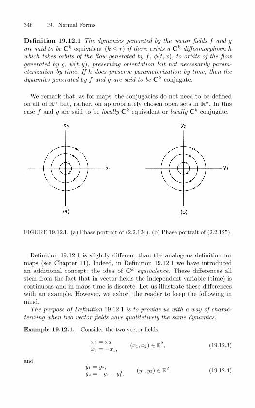
346 19. Normal Forms
Definition 19.12.1 The dynamics generated by the vector fields f and gare said to be Ck equivalent (k ≤ r) if there exists a Ck diffeomorphism hwhich takes orbits of the flow generated by f , φ(t, x), to orbits of the flow
generated by g, ψ(t, y), preserving orientation but not necessarily param-
eterization by time. If h does preserve parameterization by time, then the
dynamics generated by f and g are said to be Ck conjugate.
We remark that, as for maps, the conjugacies do not need to be definedon all of R
n but, rather, on appropriately chosen open sets in Rn. In this
case f and g are said to be locally Ck equivalent or locally Ck conjugate.
FIGURE 19.12.1. (a) Phase portrait of (2.2.124). (b) Phase portrait of (2.2.125).
Definition 19.12.1 is slightly different than the analogous definition formaps (see Chapter 11). Indeed, in Definition 19.12.1 we have introducedan additional concept: the idea of Ck equivalence. These differences allstem from the fact that in vector fields the independent variable (time) iscontinuous and in maps time is discrete. Let us illustrate these differenceswith an example. However, we exhort the reader to keep the following inmind.
The purpose of Definition 19.12.1 is to provide us with a way of charac-
terizing when two vector fields have qualitatively the same dynamics.
Example 19.12.1. Consider the two vector fields
x1 = x2,x2 = −x1,
(x1, x2) ∈ R2, (19.12.3)
andy1 = y2,y2 = −y1 − y3
1 ,(y1, y2) ∈ R
2. (19.12.4)
19.12 Conjugacies and Equivalences of Vector Fields 347
The phase portraits of each vector field are shown in Figure 21.1.1. Each vector
field possesses only a single fixed point, a center at the origin. In each case the
fixed point is surrounded by a one-parameter family of periodic orbits. Note also
from Figure 21.1.1 that in each case the direction of motion along the periodic
orbits is in the same sense; therefore, qualitatively these two vector fields have
the same dynamics—the phase portraits appear identical. However, let us see if
this is reflected by the idea of Ck conjugacy.Let us denote the flow generated by (19.12.3) as
φ(t, x), x ≡ (x1, x2),
and the flow generated by (19.12.4) as
ψ(t, y), y ≡ (y1, y2).
Suppose we have found a Ck diffeomorphism, h, taking orbits of the flow gener-
ated by (19.12.3) into orbits of the flow generated by (19.12.4). Then we have
h φ(t, x) = ψ(t, h(x)
). (19.12.5)
Equation (19.12.5) reveals an immediate problem; namely, if φ(t, x) and ψ(t, y)
are periodic in t, then h φ(t, x) and ψ(t, h(x)
)must have the same period
in order for (19.12.5) to hold. However, in general, (19.12.5) cannot be satisfied.
Consider (19.12.3) and (19.12.4). The vector field (19.12.3) is linear; therefore, all
the periodic orbits have the same period. The vector field (19.12.4) is nonlinear;
therefore, the period of the periodic orbits varies with the distance from the fixed
point. Thus, (19.12.3) and (19.12.4) are not Ck conjugate (note: one can actually
compute the period of the orbits of (19.12.4) since it is a Hamiltonian vector field.
It is a tedious exercise involving elliptic integrals).
End of Example 19.12.1
It is precisely this situation from which the idea of Ck equivalence canrescue us, for rather than only having a Ck diffeomorphism that mapsorbits to orbits, we at the same time allow a reparametrization of timealong the orbit. We make this idea more quantitative as follows. Let α(x, t)be an increasing function of t along orbits (note: it must be increasing inorder to preserve orientations of orbits). Then (19.12.3) and (19.12.4) areCk equivalent if the following holds
h φ(t, x) = ψ(α(x, t), h(x)
). (19.12.6)
Equation (19.12.6) shows that orbits of the flow generated by (19.12.3) aremapped to orbits of the flow generated by (19.12.4); however, the timedependence of the image of an orbit under h may be reparametrized in anorbitally dependent manner. Finally, we remark that the term “preservingorientation” in Definition 19.12.1 refers to the fact that the direction ofmotion along an orbit is unchanged under Ck equivalence.
Let us now consider some of the dynamical consequences of Definition19.12.1.
348 19. Normal Forms
Proposition 19.12.2 Suppose f and g are Ck conjugate. Then
i) fixed points of f are mapped to fixed points of g;
ii) T -periodic orbits of f map to T -periodic orbits of g.
Proof: That f and g are Ck conjugate under h implies the following
h φ(t, x) = ψ(t, h(x)
), (19.12.7)
Dhφ = ψ. (19.12.8)
The proof of i) follows from (19.12.8) and the proof of ii) follows from(19.12.7).
Proposition 19.12.3 Suppose f and g are Ck conjugate (k ≥ 1) and
f(x0) = 0; then Df(x0) has the same eigenvalues as Dg(h(x0)
).
Proof: We have the two vector fields x = f(x), y = g(y). By differentiating(19.12.7) with respect to t we have
Dh|x f(x) = g(h(x)
). (19.12.9)
Differentiating (19.12.9) gives
D2h∣∣x
f(x) + Dh|x Df |x = Dg|h(x) Dh|x . (19.12.10)
Evaluating (19.12.10) at x0 gives
Dh|x0Df |x0
= Dg|h(x0) Dh|x0(19.12.11)
orDf |x0
= (Dh)−1∣∣x0
Dg|h(x0) Dh|x0, (19.12.12)
and, since similar matrices have equal eigenvalues, the proof is complete.
The previous two propositions dealt with Ck conjugacies. We next ex-amine the consequences of Ck equivalence under the assumption that thechange in parameterization by time along orbits is C1. The validity of thisassumption must be verified in any specific application.
Proposition 19.12.4 Suppose f and g are Ck equivalent; then
i) fixed points of f are mapped to fixed points of g;
ii) periodic orbits of f are mapped to periodic orbits of g, but the periods
need not be equal.
19.12 Conjugacies and Equivalences of Vector Fields 349
Proof: If f and g are Ck equivalent, then
h φ(t, x) = ψ(α(x, t), h(x)
), (19.12.13)
where α is an increasing function of time along orbits (note: α must beincreasing in order to preserve orientations of orbits).
Differentiating (19.12.13) gives
Dhφ =∂α
∂t
∂ψ
∂α. (19.12.14)
Therefore, (19.12.14) implies i), and ii) follows automatically since Ck dif-
feomorphisms map closed curves to closed curves. (If this were not true,then the inverse would not be continuous.)
Proposition 19.12.5 Suppose f and g are Ck equivalent (k ≥ 1)and f(x0) = 0; then the eigenvalues of Df(x0) and the eigenvalues of
Dg(h(x0)
)differ by a positive multiplicative constant.
Proof: Proceeding as in the proof of Proposition 19.12.3, we have
Dh|x f(x) =∂α
∂tg(h(x)
). (19.12.15)
Differentiating (19.12.15) gives
D2h∣∣x
f(x) + Dh|x Df |x =∂α
∂tDg|h(x) Dh|x +
∂2α
∂x∂t
∣∣∣∣x
g(h(x)
).
(19.12.16)Evaluating at x0 gives
Dh|x0Df |x0
=∂α
∂tDg|h(x0) Dh|x0
; (19.12.17)
thus, Df |x0and Dg|h(x0) are similar up to the multiplicative constant
∂α/∂t, which is positive, since α is increasing on orbits.
Example 19.12.2. Consider the vector fields
x1 = x1,x2 = x2,
(x1, x2) ∈ R2,
andy1 = y1,y2 = 2y2,
(y1, y2) ∈ R2.
Qualitatively these two vector fields have the same dynamics. However, by Propo-
sition 19.12.3 they are not Ck equivalent, k ≥ 1.
End of Example 19.12.2
350 19. Normal Forms
19.12a An Application: The Hartman-GrobmanTheorem
An underlying theme throughout the first chapter of this book was thatthe orbit structure near a hyperbolic fixed point was qualitatively the sameas the orbit structure given by the associated linearized dynamical system.A theorem proved independently by Hartman [1960] and Grobman [1959]makes this precise. We will describe the situation for vector fields.
Consider a Cr (r ≥ 1) vector field
x = f(x), x ∈ Rn, (19.12.18)
where f is defined on a sufficiently large open set of Rn. Suppose that
(19.12.18) has a hyperbolic fixed point at x = x0, i.e.,
f(x0) = 0,
and Df(x0) has no eigenvalues on the imaginary axis. Consider the asso-ciated linear vector field
ξ = Df(x0)ξ, ξ ∈ Rn. (19.12.19)
Then we have the following theorem.
Theorem 19.12.6 (Hartman and Grobman) The flow generated by
(19.12.18) is C0 conjugate to the flow generated by (19.12.19) in a neigh-
borhood of the fixed point x = x0.
Proof: See Arnold [1973] or Palis and deMelo [1982].
We remark that the theorem can be modified so that it applies to hy-perbolic fixed points of maps, and we leave it to the reader to reformulatethe theorem along these lines.
A point to note concerning Theorem 19.12.6 is that the conjugacy trans-forming the nonlinear flow into the linear flow near the hyperbolic fixedpoint is not differentiable; rather, it is a homeomorphism. This makes thegeneration of the transformation via, for example, normal form theory, notpossible since the coordinate transformations constructed via that theorywere power series expansions and, hence, differentiable. However, a closerlook at normal form theory will reveal the heart of the problem with “dif-ferentiable linearization.” Let us expand on this with a brief discussion.
Recall equation (19.1.8)
x = Jx + F2(x) + · · ·+ Fr−1(x) +O(|x|r), x ∈ Rn. (19.12.20)
A sufficient condition for eliminating the O(|x|k) terms (2 ≤ k ≤ r − 1)from (19.12.20) is that the linear operator L
(k)J (·) is invertible on Hk. We
want to explore why L(k)J (·) is noninvertible.
19.12 Conjugacies and Equivalences of Vector Fields 351
RecallL
(k)J
(hk(x)
)≡ Jhk(x)−Dhk(x)Jx, (19.12.21)
with hk(x) ∈ Hk, where Hk is the linear vector space of vector-valuedhomogeneous polynomials of degree k. Let us choose a basis for Hk. SupposeJ is diagonal with eigenvalues λ1, · · · , λn (note: if J is not diagonalizable,then the following argument is still valid, but with slight modifications; seeArnold [1983] or Bryuno [1989a]). Let ei, 1 ≤ i ≤ n, be the standard basisof R
n, i.e., ei is an n vector with a 1 in the ith component and zeros in theremaining components. Then we have
Jei = λiei. (19.12.22)
As a basis for Hk we take the set of elements
xm11 · · ·xmn
n ei,
n∑j=1
mj = k, mj ≥ 0, (19.12.23)
where we consider all possible terms xm11 · · ·xmn
n of degree k multiplyingeach ei, 1 ≤ i ≤ n.
Next we consider the action of L(k)J (·) on each of these basis elements of
Hk. Let
hk(x) = xm11 · · ·xmn
n ei,
n∑j=1
mj = k, mj ≥ 0; (19.12.24)
then a simple calculation shows that
L(k)J
(hk(x)
)= Jhk(x)−Dhk(x)Jx =
[λi −
n∑j=1
mjλj
]hk(x). (19.12.25)
Thus, the linear operator L(k)J (·) is diagonal in this basis, with eigenvalues
given by
λi −n∑
j=1
mjλj . (19.12.26)
Now we can see the problem. The linear operator L(k)J (·) will fail to be
invertible if it has a zero eigenvalue, which in this case means
λi =n∑
j=1
mjλj . (19.12.27)
Equation (19.12.27) is called a resonance and is the origin of the name“resonance terms” for the unremovable nonlinear terms in the normal formdescribed in Theorem 19.1.1. The integer
n∑j=1
mj
352 19. Normal Forms
is called the order of the resonance. Thus, the difficulty in finding a differ-entiable coordinate change that will linearize a vector field in the neighbor-hood of a hyperbolic fixed point lies in the fact that an eigenvalue of thelinearized part may be equal to a linear combination over the nonnegativeintegers of elements from the set of eigenvalues of the linearized part. Muchwork has been done on the geometry of the resonances in the complex planeand on differentiable linearizations in the situations where the resonancesare avoided. For more information we refer the reader to the fundamen-tal papers by Sternberg [1957], [1958] and also Arnold [1983] and Bryuno[1989a].
Let us consider the following example due to Sternberg (see also Meyer[1986]). Consider the vector field
x = 2x + y2,
y = y, (x, y) ∈ R2. (19.12.28)
This vector field clearly has a hyperbolic fixed point at the origin. Thevector field linearized about the origin is given by
x = 2x,
y = y. (19.12.29)
Eliminating t as the independent variable, (19.12.29) can be written as
dx
dy=
2x
y, y = 0. (19.12.30)
Solving (19.12.30), the orbits of (19.12.29) are given by
x = cy2, (19.12.31)
where c is a constant. Clearly (19.12.31) are analytic curves at the origin.Now consider the nonlinear vector field (19.12.28). Eliminating t as the
independent variable, (19.12.28) can be written as
dx
dy=
2x
y+ y, y = 0. (19.12.32)
Equation (19.12.32) is a standard first-order linear equation which can besolved via elementary methods (see, e.g., Boyce and DiPrima [1977]). Thesolution of (19.12.32) is given by
x = y2 [k + log |y|] , (19.12.33)
where k is a constant. Clearly (19.12.33) are C1 but not C2 at the origin.Since the property of lying on C2 curves must be preserved under a C2
change of coordinates (the chain rule), we conclude that (19.12.28) and(19.12.29) are C1 but not C2 conjugate.
19.13 Final Remarks on Normal Forms 353
In terms of resonances, the problem involves a second-order resonance(hence the problem with C2 linearization). This can be seen as follows. Let
λ1 = 1,
λ2 = 2,
be the eigenvalues of the linearization. Then we have
λ2 = m1λ1 + m2λ2,
with m1 = 2, m2 = 0, and∑2
j=1 mj = 2.
19.12b An Application: Dynamics Near a FixedPoint-Sositaisvili’s Theorem
Consider the parameter-dependent vector field
x = Ax + f(x, y, z, ε),y = By + g(x, y, z, ε), (x, y, z, ε) ∈ R
c × Rs × R
u × Rp,
z = Cz + h(x, y, z, ε), (19.12.34)
wheref(0, 0, 0, 0) = 0, Df(0, 0, 0, 0) = 0,g(0, 0, 0, 0) = 0, Dg(0, 0, 0, 0) = 0,h(0, 0, 0, 0) = 0, Dh(0, 0, 0, 0) = 0,
and f , g, and h are Cr (r ≥ 2) in some neighborhood of the orgin, A is ac × c matrix having eigenvalues with zero real parts, B is a s × s matrixhaving eigenvalues with negative real parts, and C is a u×u matrix havingeigenvalues with positive real parts.
The center manifold theorem tells us that near the orgin in Rc×R
s×Ru×
Rp, the flow generated by (19.12.34) is C0 conjugate to the flow generated
by the following vector field
x = w(x, ε),y = −y, (x, y, z, ε) ∈ R
c × Rs × R
u × Rp,
z = z, (19.12.35)
where w(x, ε) represents the Cr vector field on the center manifold. Theresult in this form is due to Sositaisvili [1975].
19.13 Final Remarks on Normal Forms
Nonuniqueness of Normal Forms. It should be clear from our discus-sion that normal forms need not be unique. However, it may happen
354 19. Normal Forms
that certain properties of a vector field (e.g., symmetries) must bepossessed by any normal form. Such questions are explored in Kum-mer [1971], Bryuno [1989a], van der Meer [1985], Baider and Churchill[1988], and Baider [1989].
Divergence of the Normalizing Transformations. In general, nor-mal forms are divergent. This is discussed in detail in Siegel [1941]and Bryuno [1989a]. However, this does not affect considerations oflocal stability.
Computation of Normal Forms. The book of Rand and Armbruster[1987] describes how one may implement the computation of normalforms using computer algebra. Chow et al. [1990] provide an algo-rithm for computing normal forms, as well as a MACSYMA code.Ashkenazi et al. [1992] provide the same for Hamiltonian normalforms.
The Method of Amplitude Expansions. This method has been usedfor many years in studies of hydrodynamic stability and has much incommon with the center manifold reduction. This situation has beenclarified by Coullet and Spiegel [1983].
The Homological Equation. We want to remark on some terminology.In computing the normal form of vector fields near a fixed point, theequation
Dhk(y)Jy − Jhk(y) = Fk(y)
must be solved in order to simplify the order k terms in the Taylorexpansion of the vector field. This equation is called the homological
equation (see Arnold [1983]). The analogous equation for maps is alsocalled the homological equation.
Nonautonomous Systems. Consider the situation of Cr (with r as largeas necessary) vector fields
x = f(x), x ∈ Rn. (19.13.1)
The method of normal forms as developed in this chapter can beviewed as a method for simplifying the vector field in the neighbor-hood of a fixed point. However, suppose x(t) = x(t) is a trajectoryof this vector field. Can the method of normal forms then be usedto simplify the vector field in the neighborhood of a general (time-dependent) solution? The answer is “sometimes,” but there are asso-ciated difficulties. Let
x = x(t) + y;
then (19.13.1) becomes
y = A(t)y +O(|y|2), (19.13.2)
19.13 Final Remarks on Normal Forms 355
whereA(t) ≡ Df(x(t)).
In applying the method of normal forms to (19.13.2), the fact thatA(t) is time dependent causes problems. If x(t) is periodic in t, thenA(t) is periodic. Hence, Floquet theory can be used to transform(19.13.2) to a vector field where the linear part is constant (this isdescribed in Arnold [1983]). In this case the method of normal formsas developed in this chapter can then be applied. Recently, Floquettheory has been generalized to the quasiperiodic case by Johnson[1986, 1987]; using these ideas, the normal form theory can be ap-plied in this case also. Recent results along these lines have also beenobtained by Jorba and Simo [1992], Treshchev [1995], and Jorba etal [1997]. Their results also apply to linear systems with quasiperiod-ically varying coefficients, and are computationally very efficient.
Concerning center manifold theory, Sell [1978] has proved existencetheorems for stable, unstable, and center manifolds in nonautonomoussystems.
Some very interesting work of Siegmund [2002] has recently appearedthat develops the method of normal forms for very general nonau-tonomous vector fields.
Smooth Linearization. There exists a number of results concerning dif-ferentiable coordinate changes that linearize a dynamical system (vec-tor field or diffeomorphism) in the neighborhood of an invariant man-ifold. A recent review of these results can be found in Bronstein andKopanskii [1994].
Real Normal Forms and Complex Coordinates. We have seen nu-merous examples in this chapter where the use of complex coordi-nates simplifies normal form calculations. A systematic developmentof this approach can be found in Menck [1993].
Normal Forms for Stochastic Systems. Normal form theory for sto-chastic dynamical systems has been worked out in Namachchivayaand Leng [1990] and Namachchivaya and Lin [1991].
20
Bifurcation of Fixed Points ofVector Fields
Consider the parameterized vector field
y = g(y, λ), y ∈ Rn, λ ∈ R
p, (20.0.1)
where g is a Cr function on some open set in Rn × R
p. The degree ofdifferentiability will be determined by our need to Taylor expand (20.0.1).Usually C5 will be sufficient.
Suppose (20.0.1) has a fixed point at (y, λ) = (y0, λ0), i.e.,
g(y0, λ0) = 0. (20.0.2)
Two questions immediately arise.
1. Is the fixed point stable or unstable?
2. How is the stability or instability affected as λ is varied?
To answer Question 1, the first step to take is to examine the linear vectorfield obtained by linearizing (20.0.1) about the fixed point (y, λ) = (y0, λ0).This linear vector field is given by
ξ = Dyg(y0, λ0)ξ, ξ ∈ Rn. (20.0.3)
If the fixed point is hyperbolic (i.e., none of the eigenvalues of Dyg(y0, λ0)lie on the imaginary axis), we know that the stability of (y0, λ0) in (20.0.1)is determined by the linear equation (20.0.3) (cf. Chapter 1). This alsoenables us to answer Question 2, because since hyperbolic fixed points arestructurally stable (cf. Chapter 12), varying λ slightly does not change thenature of the stability of the fixed point. This should be clear intuitively,but let us belabor the point slightly.
We know thatg(y0, λ0) = 0, (20.0.4)
and thatDyg(y0, λ0) (20.0.5)
has no eigenvalues on the imaginary axis. Therefore, Dyg(y0, λ0) is in-vertible. By the implicit function theorem, there thus exists a unique Cr
function, y(λ), such thatg(y(λ), λ) = 0 (20.0.6)
20.1 A Zero Eigenvalue 357
for λ sufficiently close to λ0 with
y(λ0) = y0. (20.0.7)
Now, by continuity of the eigenvalues with respect to parameters, for λsufficiently close to λ0,
Dyg(y(λ), λ) (20.0.8)
has no eigenvalues on the imaginary axis. Therefore, for λ sufficiently closeto λ0, the hyperbolic fixed point (y0, λ0) of (20.0.1) persists and its stabilitytype remains unchanged. To summarize, in a neighborhood of λ0 an isolatedfixed point of (20.0.1) persists and always has the same stability type.
The real fun starts when the fixed point (y0, λ0) of (20.0.1) is not hyper-bolic, i.e., when Dyg(y0, λ0) has some eigenvalues on the imaginary axis.In this case, for λ very close to λ0 (and for y close to y0), radically newdynamical behavior can occur. For example, fixed points can be created ordestroyed and time-dependent behavior such as periodic, quasiperiodic, oreven chaotic dynamics can be created. In a certain sense (to be clarifiedlater), the more eigenvalues on the imaginary axis, the more exotic thedynamics will be.
We will begin our study by considering the simplest way in whichDyg(y0, λ0) can be nonhyperbolic. This is the case where Dyg(y0, λ0) hasa single zero eigenvalue with the remaining eigenvalues having nonzero realparts. The question we ask in this situation is what is the nature of thisnonhyperbolic fixed point for λ close to λ0? It is under these circumstanceswhere the real power of the center manifold theory becomes apparent, sincewe know that this question can be answered by studying the vector field(20.0.1) restricted to the associated center manifold (cf. Section 18.2). Inthis case the vector field on the center manifold will be a p-parameter fam-ily of one-dimensional vector fields. This represents a vast simplification of(20.0.1).
20.1 A Zero Eigenvalue
Suppose that Dyg(y0, λ0) has a single zero eigenvalue with the remainingeigenvalues having nonzero real parts; then the orbit structure near (y0, λ0)is determined by the associated center manifold equation, which we writeas
x = f(x, µ), x ∈ R1, µ ∈ R
p, (20.1.1)
where µ = λ− λ0. Furthermore, we know that (20.1.1) must satisfy
f(0, 0) = 0, (20.1.2)
∂f
∂x(0, 0) = 0. (20.1.3)
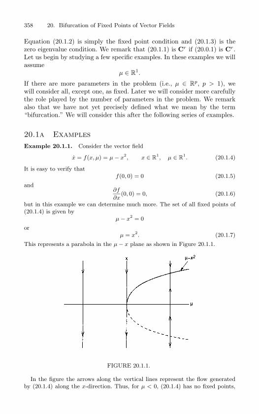
358 20. Bifurcation of Fixed Points of Vector Fields
Equation (20.1.2) is simply the fixed point condition and (20.1.3) is thezero eigenvalue condition. We remark that (20.1.1) is Cr if (20.0.1) is Cr.Let us begin by studying a few specific examples. In these examples we willassume
µ ∈ R1.
If there are more parameters in the problem (i.e., µ ∈ Rp, p > 1), we
will consider all, except one, as fixed. Later we will consider more carefullythe role played by the number of parameters in the problem. We remarkalso that we have not yet precisely defined what we mean by the term“bifurcation.” We will consider this after the following series of examples.
20.1a ExamplesExample 20.1.1. Consider the vector field
x = f(x, µ) = µ − x2, x ∈ R1, µ ∈ R
1. (20.1.4)
It is easy to verify that
f(0, 0) = 0 (20.1.5)
and∂f
∂x(0, 0) = 0, (20.1.6)
but in this example we can determine much more. The set of all fixed points of
(20.1.4) is given by
µ − x2= 0
or
µ = x2. (20.1.7)
This represents a parabola in the µ − x plane as shown in Figure 20.1.1.
FIGURE 20.1.1.
In the figure the arrows along the vertical lines represent the flow generated
by (20.1.4) along the x-direction. Thus, for µ < 0, (20.1.4) has no fixed points,
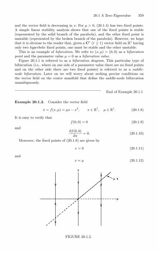
20.1 A Zero Eigenvalue 359
and the vector field is decreasing in x. For µ > 0, (20.1.4) has two fixed points.
A simple linear stability analysis shows that one of the fixed points is stable
(represented by the solid branch of the parabola), and the other fixed point is
unstable (represented by the broken branch of the parabola). However, we hope
that it is obvious to the reader that, given a Cr (r ≥ 1) vector field on R1 having
only two hyperbolic fixed points, one must be stable and the other unstable.
This is an example of bifurcation. We refer to (x, µ) = (0, 0) as a bifurcationpoint and the parameter value µ = 0 as a bifurcation value.
Figure 20.1.1 is referred to as a bifurcation diagram. This particular type of
bifurcation (i.e., where on one side of a parameter value there are no fixed points
and on the other side there are two fixed points) is referred to as a saddle-node bifurcation. Later on we will worry about seeking precise conditions on
the vector field on the center manifold that define the saddle-node bifurcation
unambiguously.
End of Example 20.1.1
Example 20.1.2. Consider the vector field
x = f(x, µ) = µx − x2, x ∈ R1, µ ∈ R
1. (20.1.8)
It is easy to verify that
f(0, 0) = 0 (20.1.9)
and∂f(0, 0)
∂x= 0. (20.1.10)
Moreover, the fixed points of (20.1.8) are given by
x = 0 (20.1.11)
and
x = µ (20.1.12)
FIGURE 20.1.2.
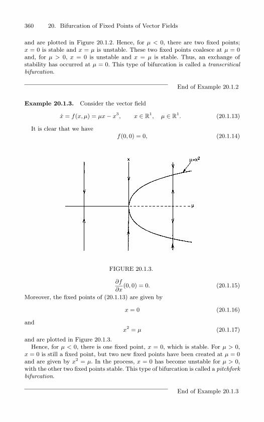
360 20. Bifurcation of Fixed Points of Vector Fields
and are plotted in Figure 20.1.2. Hence, for µ < 0, there are two fixed points;
x = 0 is stable and x = µ is unstable. These two fixed points coalesce at µ = 0
and, for µ > 0, x = 0 is unstable and x = µ is stable. Thus, an exchange of
stability has occurred at µ = 0. This type of bifurcation is called a transcriticalbifurcation.
End of Example 20.1.2
Example 20.1.3. Consider the vector field
x = f(x, µ) = µx − x3, x ∈ R1, µ ∈ R
1. (20.1.13)
It is clear that we have
f(0, 0) = 0, (20.1.14)
FIGURE 20.1.3.
∂f
∂x(0, 0) = 0. (20.1.15)
Moreover, the fixed points of (20.1.13) are given by
x = 0 (20.1.16)
and
x2= µ (20.1.17)
and are plotted in Figure 20.1.3.
Hence, for µ < 0, there is one fixed point, x = 0, which is stable. For µ > 0,
x = 0 is still a fixed point, but two new fixed points have been created at µ = 0
and are given by x2 = µ. In the process, x = 0 has become unstable for µ > 0,
with the other two fixed points stable. This type of bifurcation is called a pitchforkbifurcation.
End of Example 20.1.3
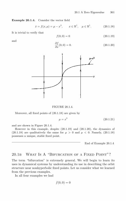
20.1 A Zero Eigenvalue 361
Example 20.1.4. Consider the vector field
x = f(x, µ) = µ − x3, x ∈ R1, µ ∈ R
1. (20.1.18)
It is trivial to verify that
f(0, 0) = 0 (20.1.19)
and∂f
∂x(0, 0) = 0. (20.1.20)
FIGURE 20.1.4.
Moreover, all fixed points of (20.1.18) are given by
µ = x3(20.1.21)
and are shown in Figure 20.1.4.
However in this example, despite (20.1.19) and (20.1.20), the dynamics of
(20.1.18) are qualitatively the same for µ > 0 and µ < 0. Namely, (20.1.18)
possesses a unique, stable fixed point.
End of Example 20.1.4
20.1b What Is A “Bifurcation of a Fixed Point”?The term “bifurcation” is extremely general. We will begin to learn itsuses in dynamical systems by understanding its use in describing the orbitstructure near nonhyperbolic fixed points. Let us consider what we learnedfrom the previous examples.
In all four examples we had
f(0, 0) = 0
362 20. Bifurcation of Fixed Points of Vector Fields
and∂f
∂x(0, 0) = 0,
and yet the orbit structure near µ = 0 was different in all four cases.Hence, knowing that a fixed point has a zero eigenvalue for µ = 0 is notsufficient to determine the orbit structure for λ near zero. Let us considereach example individually.
1. (Example 20.1.1). In this example a unique curve (or branch) of fixedpoints passed through the origin. Moreover, the curve lay entirely onone side of µ = 0 in the µ− x plane.
2. (Example 20.1.2). In this example two curves of fixed points inter-sected at the origin in the µ− x plane. Both curves existed on eitherside of µ = 0. However, the stability of the fixed point along a givencurve changed on passing through µ = 0.
3. (Example 20.1.3). In this example two curves of fixed points inter-sected at the origin in the µ − x plane. Only one curve (x = 0)existed on both sides of µ = 0; however, its stability changed onpassing through µ = 0. The other curve of fixed points lay entirelyto one side of µ = 0 and had a stability type that was the oppositeof x = 0 for µ > 0.
4. (Example 20.1.4). This example had a unique curve of fixed pointspassing through the origin in the µ − x plane and existing on bothsides of µ = 0. Moreover, all fixed points along the curve had the samestability type. Hence, despite the fact that the fixed point (x, µ) =(0, 0) was nonhyperbolic, the orbit structure was qualitatively thesame for all µ.
We want to apply the term “bifurcation” to Examples 20.1.1, 20.1.2, and20.1.3 but not to Example 20.1.4 to describe the change in orbit structureas µ passes through zero. We are therefore led to the following definition.
Definition 20.1.1 (Bifurcation of a Fixed Point) A fixed point (x, µ)= (0, 0) of a one-parameter family of one-dimensional vector fields is said
to undergo a bifurcation at µ = 0 if the flow for µ near zero and x near
zero is not qualitatively the same as the flow near x = 0 at µ = 0.
Several remarks are now in order concerning this definition.
Remark 1. The phrase “qualitatively the same” is a bit vague. It can bemade precise by substituting the term “C0-equivalent” (cf. Section 19.12),and this is perfectly adequate for the study of the bifurcation of fixedpoints of one-dimensional vector fields. However, we will see that as weexplore higher dimensional phase spaces and global bifurcations, how to
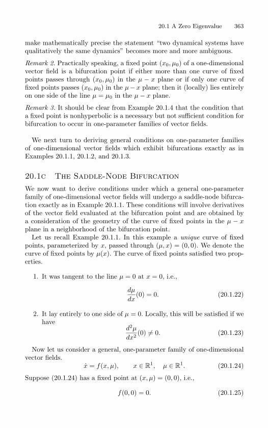
20.1 A Zero Eigenvalue 363
make mathematically precise the statement “two dynamical systems havequalitatively the same dynamics” becomes more and more ambiguous.
Remark 2. Practically speaking, a fixed point (x0, µ0) of a one-dimensionalvector field is a bifurcation point if either more than one curve of fixedpoints passes through (x0, µ0) in the µ − x plane or if only one curve offixed points passes (x0, µ0) in the µ−x plane; then it (locally) lies entirelyon one side of the line µ = µ0 in the µ− x plane.
Remark 3. It should be clear from Example 20.1.4 that the condition thata fixed point is nonhyperbolic is a necessary but not sufficient condition forbifurcation to occur in one-parameter families of vector fields.
We next turn to deriving general conditions on one-parameter familiesof one-dimensional vector fields which exhibit bifurcations exactly as inExamples 20.1.1, 20.1.2, and 20.1.3.
20.1c The Saddle-Node BifurcationWe now want to derive conditions under which a general one-parameterfamily of one-dimensional vector fields will undergo a saddle-node bifurca-tion exactly as in Example 20.1.1. These conditions will involve derivativesof the vector field evaluated at the bifurcation point and are obtained bya consideration of the geometry of the curve of fixed points in the µ − xplane in a neighborhood of the bifurcation point.
Let us recall Example 20.1.1. In this example a unique curve of fixedpoints, parameterized by x, passed through (µ, x) = (0, 0). We denote thecurve of fixed points by µ(x). The curve of fixed points satisfied two prop-erties.
1. It was tangent to the line µ = 0 at x = 0, i.e.,
dµ
dx(0) = 0. (20.1.22)
2. It lay entirely to one side of µ = 0. Locally, this will be satisfied if wehave
d2µ
dx2 (0) = 0. (20.1.23)
Now let us consider a general, one-parameter family of one-dimensionalvector fields.
x = f(x, µ), x ∈ R1, µ ∈ R
1. (20.1.24)
Suppose (20.1.24) has a fixed point at (x, µ) = (0, 0), i.e.,
f(0, 0) = 0. (20.1.25)
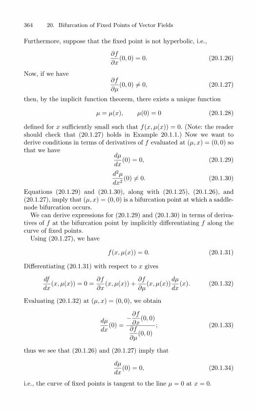
364 20. Bifurcation of Fixed Points of Vector Fields
Furthermore, suppose that the fixed point is not hyperbolic, i.e.,
∂f
∂x(0, 0) = 0. (20.1.26)
Now, if we have∂f
∂µ(0, 0) = 0, (20.1.27)
then, by the implicit function theorem, there exists a unique function
µ = µ(x), µ(0) = 0 (20.1.28)
defined for x sufficiently small such that f(x, µ(x)) = 0. (Note: the readershould check that (20.1.27) holds in Example 20.1.1.) Now we want toderive conditions in terms of derivatives of f evaluated at (µ, x) = (0, 0) sothat we have
dµ
dx(0) = 0, (20.1.29)
d2µ
dx2 (0) = 0. (20.1.30)
Equations (20.1.29) and (20.1.30), along with (20.1.25), (20.1.26), and(20.1.27), imply that (µ, x) = (0, 0) is a bifurcation point at which a saddle-node bifurcation occurs.
We can derive expressions for (20.1.29) and (20.1.30) in terms of deriva-tives of f at the bifurcation point by implicitly differentiating f along thecurve of fixed points.
Using (20.1.27), we have
f(x, µ(x)) = 0. (20.1.31)
Differentiating (20.1.31) with respect to x gives
df
dx(x, µ(x)) = 0 =
∂f
∂x(x, µ(x)) +
∂f
∂µ(x, µ(x))
dµ
dx(x). (20.1.32)
Evaluating (20.1.32) at (µ, x) = (0, 0), we obtain
dµ
dx(0) =
−∂f
∂x(0, 0)
∂f
∂µ(0, 0)
; (20.1.33)
thus we see that (20.1.26) and (20.1.27) imply that
dµ
dx(0) = 0, (20.1.34)
i.e., the curve of fixed points is tangent to the line µ = 0 at x = 0.
20.1 A Zero Eigenvalue 365
FIGURE 20.1.5.
a)(− ∂2f
∂x2 (0, 0)/ ∂f∂µ
(0, 0))
> 0; b)(− ∂2f
∂x2 (0, 0)/ ∂f∂µ
(0, 0))
< 0.
Next, let us differentiate (20.1.32) once more with respect to x to obtain
d2f
dx2 (x, µ(x)) = 0 =∂2f
∂x2 (x, µ(x)) + 2∂2f
∂x∂µ(x, µ(x))
dµ
dx(x)
+∂2f
∂µ2 (x, µ(x))(
dµ
dx(x)
)2
+∂f
∂µ(µ, µ(x))
d2µ
dx2 (x). (20.1.35)
Evaluating (20.1.35) at (µ, x) = (0, 0) and using (20.1.33) gives
∂2f
∂x2 (0, 0) +∂f
∂µ(0, 0)
d2µ
dx2 (0) = 0
or
d2µ
dx2 (0) =−∂2f
∂x2 (0, 0)
∂f
∂µ(0, 0)
. (20.1.36)
Hence, (20.1.36) is nonzero provided we have
∂2f
∂x2 (0, 0) = 0. (20.1.37)
366 20. Bifurcation of Fixed Points of Vector Fields
Let us summarize. In order for (20.1.24) to undergo a saddle-node bifur-cation we must have
f(0, 0) = 0
∂f
∂x(0, 0) = 0
nonhyperbolic fixed point (20.1.38)
and∂f
∂µ(0, 0) = 0, (20.1.39)
∂2f
∂x2 (0, 0) = 0. (20.1.40)
Equation (20.1.39) implies that a unique curve of fixed points passesthrough (µ, x) = (0, 0), and (20.1.40) implies that the curve lies locally onone side of µ = 0. It should be clear that the sign of (20.1.36) determineson which side of µ = 0 the curve lies. In Figure 20.1.5 we show both caseswithout indicating stability and leave it as an exercise for the reader toverify the stability types of the different branches of fixed points emanatingfrom the bifurcation point.
Let us end our discussion of the saddle-node bifurcation with the follow-ing remark. Consider a general one-parameter family of one-dimensionalvector fields having a nonhyperbolic fixed point at (x, µ) = (0, 0). TheTaylor expansion of this vector field is given as follows
f(x, µ) = a0µ + a1x2 + a2µx + a3µ
2 +O(3). (20.1.41)
Our computations show that the dynamics of (20.1.41) near (µ, x) = (0, 0)are qualitatively the same as one of the following vector fields
x = µ± x2. (20.1.42)
Hence, (20.1.42) can be viewed as the normal form for saddle-node bifur-cations.
This brings up another important point. In applying the method of nor-mal forms there is always the question of truncation of the normal form;namely, how are the dynamics of the normal form including only the O(k)terms modified when the higher order terms are included? We see that,in the study of the saddle-node bifurcation, all terms of O(3) and highercould be neglected and the dynamics would not be qualitatively changed.The implicit function theorem was the tool that enabled us to verify thisfact.
20.1d The Transcritical BifurcationWe want to follow the same strategy as in our discussion and derivationof general conditions for the saddle-node bifurcation given in the previous
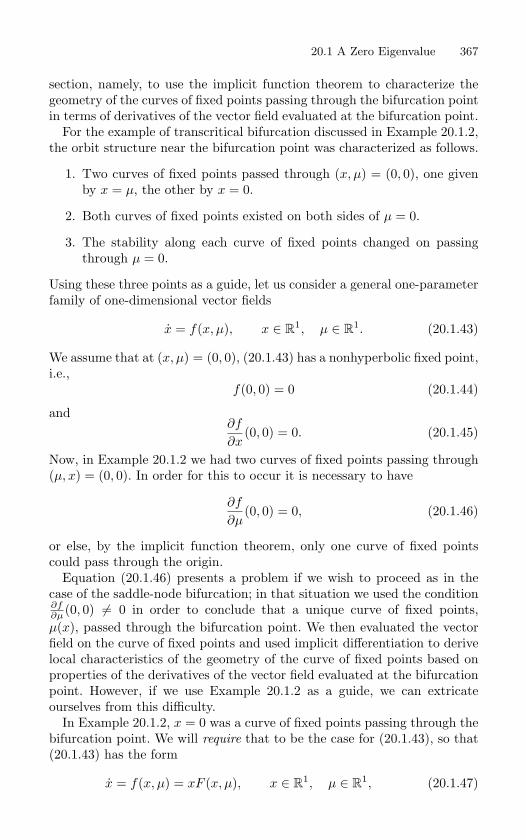
20.1 A Zero Eigenvalue 367
section, namely, to use the implicit function theorem to characterize thegeometry of the curves of fixed points passing through the bifurcation pointin terms of derivatives of the vector field evaluated at the bifurcation point.
For the example of transcritical bifurcation discussed in Example 20.1.2,the orbit structure near the bifurcation point was characterized as follows.
1. Two curves of fixed points passed through (x, µ) = (0, 0), one givenby x = µ, the other by x = 0.
2. Both curves of fixed points existed on both sides of µ = 0.
3. The stability along each curve of fixed points changed on passingthrough µ = 0.
Using these three points as a guide, let us consider a general one-parameterfamily of one-dimensional vector fields
x = f(x, µ), x ∈ R1, µ ∈ R
1. (20.1.43)
We assume that at (x, µ) = (0, 0), (20.1.43) has a nonhyperbolic fixed point,i.e.,
f(0, 0) = 0 (20.1.44)
and∂f
∂x(0, 0) = 0. (20.1.45)
Now, in Example 20.1.2 we had two curves of fixed points passing through(µ, x) = (0, 0). In order for this to occur it is necessary to have
∂f
∂µ(0, 0) = 0, (20.1.46)
or else, by the implicit function theorem, only one curve of fixed pointscould pass through the origin.
Equation (20.1.46) presents a problem if we wish to proceed as in thecase of the saddle-node bifurcation; in that situation we used the condition∂f∂µ (0, 0) = 0 in order to conclude that a unique curve of fixed points,µ(x), passed through the bifurcation point. We then evaluated the vectorfield on the curve of fixed points and used implicit differentiation to derivelocal characteristics of the geometry of the curve of fixed points based onproperties of the derivatives of the vector field evaluated at the bifurcationpoint. However, if we use Example 20.1.2 as a guide, we can extricateourselves from this difficulty.
In Example 20.1.2, x = 0 was a curve of fixed points passing through thebifurcation point. We will require that to be the case for (20.1.43), so that(20.1.43) has the form
x = f(x, µ) = xF (x, µ), x ∈ R1, µ ∈ R
1, (20.1.47)
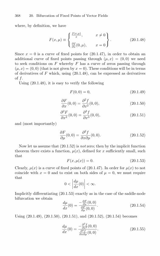
368 20. Bifurcation of Fixed Points of Vector Fields
where, by definition, we have
F (x, µ) ≡
f(x,µ)x , x = 0
∂f∂x (0, µ), x = 0
. (20.1.48)
Since x = 0 is a curve of fixed points for (20.1.47), in order to obtain anadditional curve of fixed points passing through (µ, x) = (0, 0) we needto seek conditions on F whereby F has a curve of zeros passing through(µ, x) = (0, 0) (that is not given by x = 0). These conditions will be in termsof derivatives of F which, using (20.1.48), can be expressed as derivativesof f .
Using (20.1.48), it is easy to verify the following
F (0, 0) = 0, (20.1.49)
∂F
∂x(0, 0) =
∂2f
∂x2 (0, 0), (20.1.50)
∂2F
∂x2 (0, 0) =∂3f
∂x3 (0, 0), (20.1.51)
and (most importantly)
∂F
∂µ(0, 0) =
∂2f
∂x∂µ(0, 0). (20.1.52)
Now let us assume that (20.1.52) is not zero; then by the implicit functiontheorem there exists a function, µ(x), defined for x sufficiently small, suchthat
F (x, µ(x)) = 0. (20.1.53)
Clearly, µ(x) is a curve of fixed points of (20.1.47). In order for µ(x) to notcoincide with x = 0 and to exist on both sides of µ = 0, we must requirethat
0 <
∣∣∣∣dµ
dx(0)
∣∣∣∣ < ∞.
Implicitly differentiating (20.1.53) exactly as in the case of the saddle-nodebifurcation we obtain
dµ
dx(0) =
−∂F∂x (0, 0)
∂F∂µ (0, 0)
. (20.1.54)
Using (20.1.49), (20.1.50), (20.1.51), and (20.1.52), (20.1.54) becomes
dµ
dx(0) =
−∂2f∂x2 (0, 0)
∂2f∂x∂µ (0, 0)
. (20.1.55)
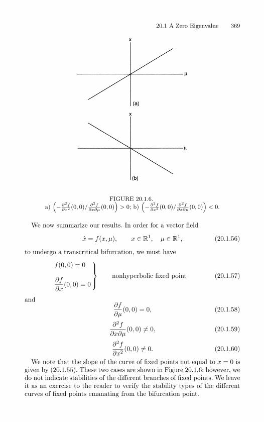
20.1 A Zero Eigenvalue 369
FIGURE 20.1.6.
a)(− ∂2f
∂x2 (0, 0)/ ∂2f∂x∂µ
(0, 0))
> 0; b)(− ∂2f
∂x2 (0, 0)/ ∂2f∂x∂µ
(0, 0))
< 0.
We now summarize our results. In order for a vector field
x = f(x, µ), x ∈ R1, µ ∈ R
1, (20.1.56)
to undergo a transcritical bifurcation, we must have
f(0, 0) = 0
∂f
∂x(0, 0) = 0
nonhyperbolic fixed point (20.1.57)
and∂f
∂µ(0, 0) = 0, (20.1.58)
∂2f
∂x∂µ(0, 0) = 0, (20.1.59)
∂2f
∂x2 (0, 0) = 0. (20.1.60)
We note that the slope of the curve of fixed points not equal to x = 0 isgiven by (20.1.55). These two cases are shown in Figure 20.1.6; however, wedo not indicate stabilities of the different branches of fixed points. We leaveit as an exercise to the reader to verify the stability types of the differentcurves of fixed points emanating from the bifurcation point.
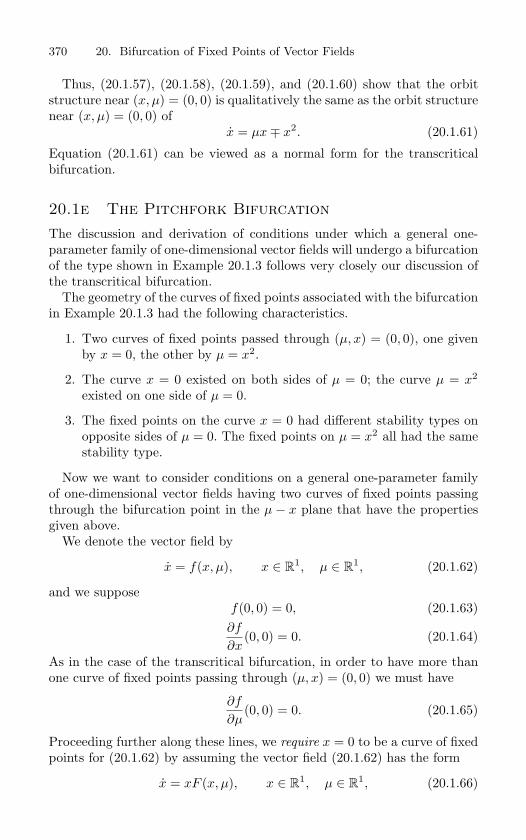
370 20. Bifurcation of Fixed Points of Vector Fields
Thus, (20.1.57), (20.1.58), (20.1.59), and (20.1.60) show that the orbitstructure near (x, µ) = (0, 0) is qualitatively the same as the orbit structurenear (x, µ) = (0, 0) of
x = µx∓ x2. (20.1.61)
Equation (20.1.61) can be viewed as a normal form for the transcriticalbifurcation.
20.1e The Pitchfork BifurcationThe discussion and derivation of conditions under which a general one-parameter family of one-dimensional vector fields will undergo a bifurcationof the type shown in Example 20.1.3 follows very closely our discussion ofthe transcritical bifurcation.
The geometry of the curves of fixed points associated with the bifurcationin Example 20.1.3 had the following characteristics.
1. Two curves of fixed points passed through (µ, x) = (0, 0), one givenby x = 0, the other by µ = x2.
2. The curve x = 0 existed on both sides of µ = 0; the curve µ = x2
existed on one side of µ = 0.
3. The fixed points on the curve x = 0 had different stability types onopposite sides of µ = 0. The fixed points on µ = x2 all had the samestability type.
Now we want to consider conditions on a general one-parameter familyof one-dimensional vector fields having two curves of fixed points passingthrough the bifurcation point in the µ − x plane that have the propertiesgiven above.
We denote the vector field by
x = f(x, µ), x ∈ R1, µ ∈ R
1, (20.1.62)
and we supposef(0, 0) = 0, (20.1.63)∂f
∂x(0, 0) = 0. (20.1.64)
As in the case of the transcritical bifurcation, in order to have more thanone curve of fixed points passing through (µ, x) = (0, 0) we must have
∂f
∂µ(0, 0) = 0. (20.1.65)
Proceeding further along these lines, we require x = 0 to be a curve of fixedpoints for (20.1.62) by assuming the vector field (20.1.62) has the form
x = xF (x, µ), x ∈ R1, µ ∈ R
1, (20.1.66)
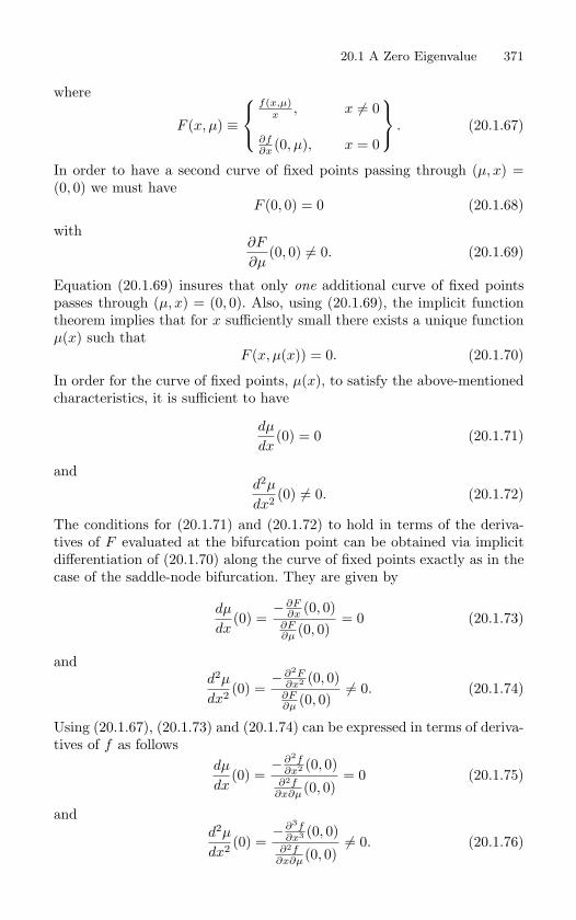
20.1 A Zero Eigenvalue 371
where
F (x, µ) ≡
f(x,µ)x , x = 0
∂f∂x (0, µ), x = 0
. (20.1.67)
In order to have a second curve of fixed points passing through (µ, x) =(0, 0) we must have
F (0, 0) = 0 (20.1.68)
with∂F
∂µ(0, 0) = 0. (20.1.69)
Equation (20.1.69) insures that only one additional curve of fixed pointspasses through (µ, x) = (0, 0). Also, using (20.1.69), the implicit functiontheorem implies that for x sufficiently small there exists a unique functionµ(x) such that
F (x, µ(x)) = 0. (20.1.70)
In order for the curve of fixed points, µ(x), to satisfy the above-mentionedcharacteristics, it is sufficient to have
dµ
dx(0) = 0 (20.1.71)
andd2µ
dx2 (0) = 0. (20.1.72)
The conditions for (20.1.71) and (20.1.72) to hold in terms of the deriva-tives of F evaluated at the bifurcation point can be obtained via implicitdifferentiation of (20.1.70) along the curve of fixed points exactly as in thecase of the saddle-node bifurcation. They are given by
dµ
dx(0) =
−∂F∂x (0, 0)
∂F∂µ (0, 0)
= 0 (20.1.73)
andd2µ
dx2 (0) =−∂2F
∂x2 (0, 0)∂F∂µ (0, 0)
= 0. (20.1.74)
Using (20.1.67), (20.1.73) and (20.1.74) can be expressed in terms of deriva-tives of f as follows
dµ
dx(0) =
−∂2f∂x2 (0, 0)
∂2f∂x∂µ (0, 0)
= 0 (20.1.75)
andd2µ
dx2 (0) =−∂3f
∂x3 (0, 0)∂2f
∂x∂µ (0, 0) = 0. (20.1.76)
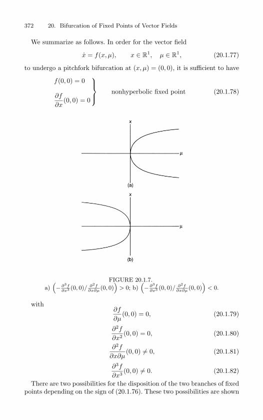
372 20. Bifurcation of Fixed Points of Vector Fields
We summarize as follows. In order for the vector field
x = f(x, µ), x ∈ R1, µ ∈ R
1, (20.1.77)
to undergo a pitchfork bifurcation at (x, µ) = (0, 0), it is sufficient to have
f(0, 0) = 0
∂f
∂x(0, 0) = 0
nonhyperbolic fixed point (20.1.78)
FIGURE 20.1.7.
a)(− ∂3f
∂x3 (0, 0)/ ∂2f∂x∂µ
(0, 0))
> 0; b)(− ∂3f
∂x3 (0, 0)/ ∂2f∂x∂µ
(0, 0))
< 0.
with∂f
∂µ(0, 0) = 0, (20.1.79)
∂2f
∂x2 (0, 0) = 0, (20.1.80)
∂2f
∂x∂µ(0, 0) = 0, (20.1.81)
∂3f
∂x3 (0, 0) = 0. (20.1.82)
There are two possibilities for the disposition of the two branches of fixedpoints depending on the sign of (20.1.76). These two possibilities are shown
20.1 A Zero Eigenvalue 373
in Figure 20.1.7 without indicating stabilities. We leave it as an exercise forthe reader to verify the stability types for the different branches of fixedpoints emanating from the bifurcation point.
We conclude by noting that (20.1.78), (20.1.79), (20.1.80), (20.1.81), and(20.1.82) imply that the orbit structure near (x, µ) = (0, 0) is qualitativelythe same as the orbit structure near (x, µ) = (0, 0) in the vector field
x = µx∓ x3. (20.1.83)
Thus, (20.1.83) can be viewed as a normal form for the pitchfork bifurca-tion.
20.1f Exercises1. In our development of the transcritical and pitchfork bifurcations we assumed that
x = 0 was a trivial solution. Was this necessary? In particular, would the conditionsfor transcritical and pitchfork bifurcations change if this were not the case?
2. Consider a Cr (r ≥ 1) autonomous vector field on R1 having precisely two hyperbolic
fixed points. Can you infer the nature of the stability of the two fixed points? Howdoes the situation change if one of the fixed points is not hyperbolic? Can both fixedpoints be nonhyperbolic? Construct explicit examples illustrating each situation.
3. Consider the saddle-node bifurcation for vector fields and Figure 20.1.5. For the case(− ∂2f
∂x2 (0, 0)/ ∂f∂µ (0, 0)
)> 0, give conditions under which the upper part of the curve
of fixed points is stable and the lower part is unstable. Alternatively, give conditionsunder which the upper part of the curve of fixed points is unstable and the lower partis stable.
Repeat the exercise for the case(
− ∂2f
∂x2 (0, 0)/ ∂f∂µ (0, 0)
)< 0.
4. Consider the transcritical bifurcation for vector fields and Figure 20.1.6. For the case(− ∂2f
∂x2 (0, 0)/ ∂2f∂x∂µ (0, 0)
)> 0, give conditions for x = 0 to be stable for µ > 0 and
unstable for µ < 0. Alternatively, give conditions for x = 0 to be unstable for µ > 0and stable for µ < 0.
Repeat the exercise for the case(
− ∂2f
∂x2 (0, 0)/ ∂2f∂x∂µ (0, 0)
)< 0.
5. Consider the pitchfork bifurcation for vector fields and Figure 20.1.7. For the case(− ∂3f
∂x3 (0, 0)/ ∂2f∂x∂µ (0, 0)
)> 0, give conditions for x = 0 to be stable for µ > 0 and
unstable for µ < 0. Alternatively, give conditions for x = 0 to be unstable for µ > 0and stable for µ < 0.
Repeat the exercise for the case(
− ∂3f
∂x3 (0, 0)/ ∂2f∂x∂µ (0, 0)
)< 0.
6. In Exercise 4 following Chapter 18 we computed center manifolds near the origin forthe following one-parameter families of vector fields. Describe the bifurcations of theorigin. In, for example, a) and a′) the parameter ε multiplies a linear and nonlinearterm, respectively. In terms of bifurcations, is there a qualitative difference in the twocases? What kinds of general statements can you make?
a) θ = −θ + εv + v2,
v = − sin θ,(θ, v) ∈ S
1 × R1.
a′) θ = −θ + v2 + εv
2,
v = − sin θ.
374 20. Bifurcation of Fixed Points of Vector Fields
b) x =12
x + y + x2y,
y = x + 2y + εy + y2,
(x, y) ∈ R2.
b′) x =12
x + y + x2y,
y = x + 2y + y2 + εy
2.
d)x = 2x + 2y + εy,
y = x + y + x4,
(x, y) ∈ R2.
d′)x = 2x + 2y,
y = x + y + x4 + εy
2.
f) x = −2x + 3y + εx + y3,
y = 2x − 3y + x3,
(x, y) ∈ R2.
f′) x = −2x + 3y + y3 + εx
2,
y = 2x − 3y + x3.
h)x = −x + y,
y = −ex + e
−x + 2x + εy,(x, y) ∈ R
2.
h′) x = −x + y + εx2,
y = −ex + e
−x + 2x.
i)x = −2x + y + z + εx + y
2z,
y = x − 2y + z + εx + xz2,
z = x + y − 2z + εx + x2y,
(x, y, z) ∈ R3.
i′)x = −2x + y + z + εx
2 + y2z,
y = x − 2y + z + εxy + xz2,
z = x + y − 2z + x2y.
j)x = −x − y + z
2,
y = 2x + y + εy − z2,
z = x + 2y − z,
(x, y, z) ∈ R3.
j′)x = −x − y + εx
2 + z2,
y = 2x + y − z2 + εy
2,
z = x + 2y − z.
k)x = −x − y − z + εx − yz,y = −x − y − z − xz,z = −x − y − z − yz,
(x, y, z) ∈ R3.
k′)x = −x − y − z − yz + εx
2,
y = −x − y − z − xz,z = −x − y − z − xy.
l) x = y + x2 + εy,
y = −y − x2,
(x, y) ∈ R2.
l′) x = y + x2 + εy
2,
y = −y − x2.
m) x = x2 + εy,
y = −y − x2,
(x, y) ∈ R2.
m′) x = x2 + εy
2,
y − −y − x2.
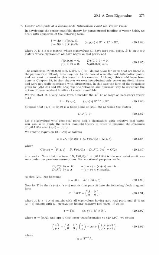
20.1 A Zero Eigenvalue 375
7. Center Manifolds at a Saddle-node Bifurcation Point for Vector Fields
In developing the center manifold theory for parametrized families of vector fields, wedealt with equations of the following form
x = Ax + f(x, y, ε),y = By + g(x, y, ε), (x, y, ε) ∈ R
c × Rs × R
p, (20.1.84)
where A is a c × c matrix whose eigenvalues all have zero real parts, B is an s × smatrix whose eigenvalues all have negative real parts, and
f(0, 0, 0) = 0, Df(0, 0, 0) = 0,g(0, 0, 0) = 0, Dg(0, 0, 0) = 0.
(20.1.85)
The conditions Df(0, 0, 0) = 0, Dg(0, 0, 0) = 0 do not allow for terms that are linear inthe parameter ε. Clearly, this may not be the case at a saddle-node bifurcation point,and we want to consider this issue in this exercise. Although this could have beendone in Chapter 18, in that chapter we were introducing only center manifold theoryand were not really concerned with bifurcations. In this case the form of the equationsgiven by (20.1.84) and (20.1.85) was the “cleanest and quickest” way to introduce thenotion of parametrized families of center manifolds.
We will start at a very basic level. Consider the Cr (r as large as necessary) vectorfield
z = F (z, ε), (z, ε) ∈ Rc+s × R
p. (20.1.86)
Suppose that (z, ε) = (0, 0) is a fixed point of (20.1.86) at which the matrix
DzF (0, 0) (20.1.87)
has c eigenvalues with zero real parts and s eigenvalues with negative real parts.Our goal is to apply the center manifold theory in order to examine the dynamicsof (20.1.86) near (z, ε) = (0, 0).
We rewrite Equation (20.1.86) as follows
z = DzF (0, 0)z + DεF (0, 0)ε + G(z, ε), (20.1.88)
whereG(z, ε) =
[F (z, ε) − DzF (0, 0)z − DεF (0, 0)ε
]= O(2) (20.1.89)
in z and ε. Note that the term “DεF (0, 0)ε” in (20.1.88) is the new wrinkle—it waszero under our previous assumptions. For notational purposes we let
DzF (0, 0) ≡ M −(c + s) × (c + s) matrix,DεF (0, 0) ≡ Λ −(c + s) × p matrix,
so that (20.1.88) becomesz = Mz + Λε + G(z, ε). (20.1.90)
Now let T be the (s+c)× (s+c) matrix that puts M into the following block diagonalform
T−1
MT =(
A 00 B
), (20.1.91)
where A is a (c × c) matrix with all eigenvalues having zero real parts and B is an(s × s) matrix with all eigenvalues having negative real parts. If we let
z = Tw, (x, y) ∈ Rc × R
s, (20.1.92)
where w = (x, y), and apply this linear transformation to (20.1.90), we obtain
(xy
)=(
A 00 B
)(xy
)+ Λε +
(f(x, y, ε)g(x, y, ε)
), (20.1.93)
whereΛ ≡ T
−1Λ,
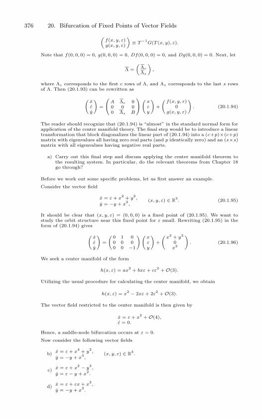
376 20. Bifurcation of Fixed Points of Vector Fields
(f(x, y, ε)g(x, y, ε)
)≡ T
−1G(T (x, y), ε).
Note that f(0, 0, 0) = 0, g(0, 0, 0) = 0, Df(0, 0, 0) = 0, and Dg(0, 0, 0) = 0. Next, let
Λ =(
Λc
Λs
),
where Λc corresponds to the first c rows of Λ, and Λs corresponds to the last s rowsof Λ. Then (20.1.93) can be rewritten as
(xεy
)=
A Λc 0
0 0 00 Λs B
(
xεy
)+
(f(x, y, ε)
0g(x, y, ε)
). (20.1.94)
The reader should recognize that (20.1.94) is “almost” in the standard normal form forapplication of the center manifold theory. The final step would be to introduce a lineartransformation that block diagonalizes the linear part of (20.1.94) into a (c+p)×(c+p)matrix with eigenvalues all having zero real parts (and p identically zero) and an (s×s)matrix with all eigenvalues having negative real parts.
a) Carry out this final step and discuss applying the center manifold theorem tothe resulting system. In particular, do the relevant theorems from Chapter 18go through?
Before we work out some specific problems, let us first answer an example.
Consider the vector field
x = ε + x2 + y
2,
y = −y + x2,
(x, y, ε) ∈ R3. (20.1.95)
It should be clear that (x, y, ε) = (0, 0, 0) is a fixed point of (20.1.95). We want tostudy the orbit structure near this fixed point for ε small. Rewriting (20.1.95) in theform of (20.1.94) gives
(xεy
)=
( 0 1 00 0 00 0 −1
)(xεy
)+
(x2 + y2
0x2
). (20.1.96)
We seek a center manifold of the form
h(x, ε) = ax2 + bxε + cε
2 + O(3).
Utilizing the usual procedure for calculating the center manifold, we obtain
h(x, ε) = x2 − 2xε + 2ε
2 + O(3).
The vector field restricted to the center manifold is then given by
x = ε + x2 + O(4),
ε = 0.
Hence, a saddle-node bifurcation occurs at ε = 0.
Now consider the following vector fields
b) x = ε + x4 + y
2,
y = −y + x3,
(x, y, ε) ∈ R3.
c) x = ε + x2 − y
3,
y = ε − y + x2.
d) x = ε + εx + x2,
y = −y + x2.
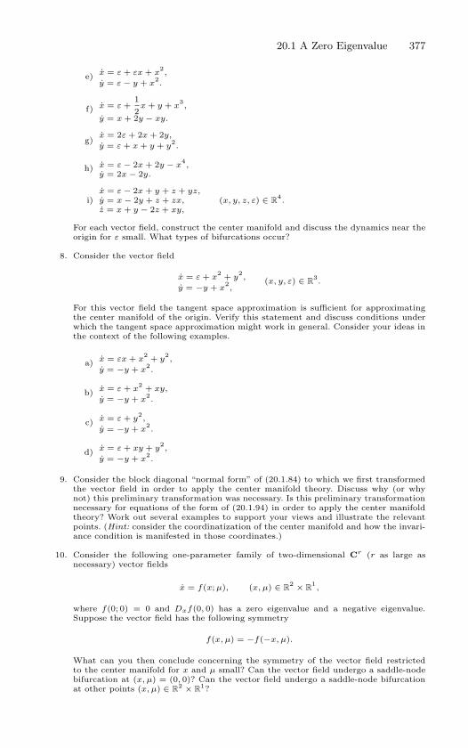
20.1 A Zero Eigenvalue 377
e) x = ε + εx + x2,
y = ε − y + x2.
f) x = ε +12
x + y + x3,
y = x + 2y − xy.
g)x = 2ε + 2x + 2y,
y = ε + x + y + y2.
h) x = ε − 2x + 2y − x4,
y = 2x − 2y.
i)x = ε − 2x + y + z + yz,y = x − 2y + z + zx,z = x + y − 2z + xy,
(x, y, z, ε) ∈ R4.
For each vector field, construct the center manifold and discuss the dynamics near theorigin for ε small. What types of bifurcations occur?
8. Consider the vector field
x = ε + x2 + y
2,
y = −y + x2,
(x, y, ε) ∈ R3.
For this vector field the tangent space approximation is sufficient for approximatingthe center manifold of the origin. Verify this statement and discuss conditions underwhich the tangent space approximation might work in general. Consider your ideas inthe context of the following examples.
a) x = εx + x2 + y
2,
y = −y + x2.
b) x = ε + x2 + xy,
y = −y + x2.
c) x = ε + y2,
y = −y + x2.
d) x = ε + xy + y2,
y = −y + x2.
9. Consider the block diagonal “normal form” of (20.1.84) to which we first transformedthe vector field in order to apply the center manifold theory. Discuss why (or whynot) this preliminary transformation was necessary. Is this preliminary transformationnecessary for equations of the form of (20.1.94) in order to apply the center manifoldtheory? Work out several examples to support your views and illustrate the relevantpoints. (Hint: consider the coordinatization of the center manifold and how the invari-ance condition is manifested in those coordinates.)
10. Consider the following one-parameter family of two-dimensional Cr (r as large asnecessary) vector fields
x = f(x; µ), (x, µ) ∈ R2 × R
1,
where f(0; 0) = 0 and Dxf(0, 0) has a zero eigenvalue and a negative eigenvalue.Suppose the vector field has the following symmetry
f(x, µ) = −f(−x, µ).
What can you then conclude concerning the symmetry of the vector field restrictedto the center manifold for x and µ small? Can the vector field undergo a saddle-nodebifurcation at (x, µ) = (0, 0)? Can the vector field undergo a saddle-node bifurcationat other points (x, µ) ∈ R
2 × R1?
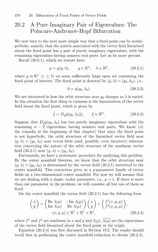
378 20. Bifurcation of Fixed Points of Vector Fields
20.2 A Pure Imaginary Pair of Eigenvalues: ThePoincare-Andronov-Hopf Bifurcation
We now turn to the next most simple way that a fixed point can be nonhy-perbolic; namely, that the matrix associated with the vector field linearizedabout the fixed point has a pair of purely imaginary eigenvalues, with theremaining eigenvalues having nonzero real parts. Let us be more precise.
Recall (20.0.1), which we restate here;
y = g(y, λ), y ∈ Rn, λ ∈ R
p, (20.2.1)
where g is Cr (r ≥ 5) on some sufficiently large open set containing thefixed point of interest. The fixed point is denoted by (y, λ) = (y0, λ0), i.e.,
0 = g(y0, λ0). (20.2.2)
We are interested in how the orbit structure near y0 changes as λ is varied.In this situation the first thing to examine is the linearization of the vectorfield about the fixed point, which is given by
ξ = Dyg(y0, λ0)ξ, ξ ∈ Rn. (20.2.3)
Suppose that Dyg(y0, λ0) has two purely imaginary eigenvalues with theremaining n − 2 eigenvalues having nonzero real parts. We know (cf.the remarks at the beginning of this chapter) that since the fixed pointis not hyperbolic, the orbit structure of the linearized vector field near(y, λ) = (y0, λ0) may reveal little (and, possibly, even incorrect) informa-tion concerning the nature of the orbit structure of the nonlinear vectorfield (20.2.1) near (y, λ) = (y0, λ0).
Fortunately, we have a systematic procedure for analyzing this problem.By the center manifold theorem, we know that the orbit structure near(y, λ) = (y0, λ0) is determined by the vector field (20.2.1) restricted to thecenter manifold. This restriction gives us a p-parameter family of vectorfields on a two-dimensional center manifold. For now we will assume thatwe are dealing with a single, scalar parameter, i.e., p = 1. If there is morethan one parameter in the problem, we will consider all but one of them asfixed.
On the center manifold the vector field (20.2.1) has the following form(xy
)=
(Re λ(µ) −Im λ(µ)Im λ(µ) Re λ(µ)
)(xy
)+
(f1(x, y, µ)f2(x, y, µ)
),
(x, y, µ) ∈ R1 × R
1 × R1, (20.2.4)
where f1 and f2 are nonlinear in x and y and λ(µ), λ(µ) are the eigenvaluesof the vector field linearized about the fixed point at the origin.
Equation (20.2.4) was first discussed in Section 19.2. The reader shouldrecall that in performing the center manifold reduction to obtain (20.2.4),
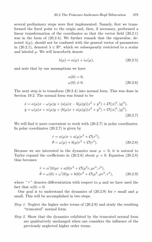
20.2 The Poincare-Andronov-Hopf Bifurcation 379
several preliminary steps were first implemented. Namely, first we trans-formed the fixed point to the origin and, then, if necessary, performed alinear transformation of the coordinates so that the vector field (20.2.1)was in the form of (20.2.4). We further remark that the eigenvalue, de-noted λ(µ), should not be confused with the general vector of parametersin (20.2.1), denoted λ ∈ R
p, which we subsequently restricted to a scalarand labeled µ. We will henceforth denote
λ(µ) = α(µ) + iω(µ), (20.2.5)
and note that by our assumptions we have
α(0) = 0,
ω(0) = 0. (20.2.6)
The next step is to transform (20.2.4) into normal form. This was done inSection 19.2. The normal form was found to be
x = α(µ)x− ω(µ)y + (a(µ)x− b(µ)y)(x2 + y2) +O(|x|5, |y|5),y = ω(µ)x + α(µ)y + (b(µ)x + a(µ)y)(x2 + y2) +O(|x|5, |y|5).
(20.2.7)
We will find it more convenient to work with (20.2.7) in polar coordinates.In polar coordinates (20.2.7) is given by
r = α(µ)r + a(µ)r3 +O(r5),θ = ω(µ) + b(µ)r2 +O(r4). (20.2.8)
Because we are interested in the dynamics near µ = 0, it is natural toTaylor expand the coefficients in (20.2.8) about µ = 0. Equation (20.2.8)thus becomes
r = α′(0)µr + a(0)r3 +O(µ2r, µr3, r5),θ = ω(0) + ω′(0)µ + b(0)r2 +O(µ2, µr2, r4), (20.2.9)
where “ ′ ” denotes differentiation with respect to µ and we have used thefact that α(0) = 0.
Our goal is to understand the dynamics of (20.2.9) for r small and µsmall. This will be accomplished in two steps.
Step 1. Neglect the higher order terms of (20.2.9) and study the resulting“truncated” normal form.
Step 2. Show that the dynamics exhibited by the truncated normal formare qualitatively unchanged when one considers the influence of thepreviously neglected higher order terms.
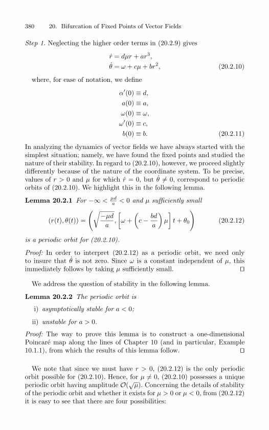
380 20. Bifurcation of Fixed Points of Vector Fields
Step 1. Neglecting the higher order terms in (20.2.9) gives
r = dµr + ar3,
θ = ω + cµ + br2, (20.2.10)
where, for ease of notation, we define
α′(0) ≡ d,
a(0) ≡ a,
ω(0) ≡ ω,
ω′(0) ≡ c,
b(0) ≡ b. (20.2.11)
In analyzing the dynamics of vector fields we have always started with thesimplest situation; namely, we have found the fixed points and studied thenature of their stability. In regard to (20.2.10), however, we proceed slightlydifferently because of the nature of the coordinate system. To be precise,values of r > 0 and µ for which r = 0, but θ = 0, correspond to periodicorbits of (20.2.10). We highlight this in the following lemma.
Lemma 20.2.1 For −∞ < µda < 0 and µ sufficiently small
(r(t), θ(t)) =
(√−µd
a,
[ω +
(c− bd
a
)µ
]t + θ0
)(20.2.12)
is a periodic orbit for (20.2.10).
Proof: In order to interpret (20.2.12) as a periodic orbit, we need onlyto insure that θ is not zero. Since ω is a constant independent of µ, thisimmediately follows by taking µ sufficiently small.
We address the question of stability in the following lemma.
Lemma 20.2.2 The periodic orbit is
i) asymptotically stable for a < 0;
ii) unstable for a > 0.
Proof: The way to prove this lemma is to construct a one-dimensionalPoincare map along the lines of Chapter 10 (and in particular, Example10.1.1), from which the results of this lemma follow.
We note that since we must have r > 0, (20.2.12) is the only periodicorbit possible for (20.2.10). Hence, for µ = 0, (20.2.10) possesses a uniqueperiodic orbit having amplitude O(
õ). Concerning the details of stability
of the periodic orbit and whether it exists for µ > 0 or µ < 0, from (20.2.12)it is easy to see that there are four possibilities:
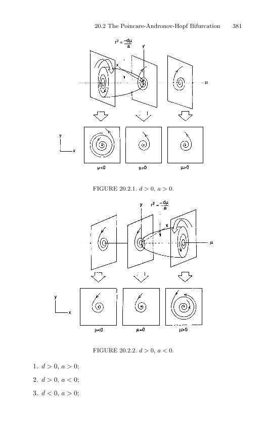
20.2 The Poincare-Andronov-Hopf Bifurcation 381
FIGURE 20.2.1. d > 0, a > 0.
FIGURE 20.2.2. d > 0, a < 0.
1. d > 0, a > 0;
2. d > 0, a < 0;
3. d < 0, a > 0;
382 20. Bifurcation of Fixed Points of Vector Fields
4. d < 0, a < 0.
We will examine each case individually; however, we note that in all casesthe origin is a fixed point which is
stable at µ = 0 for a < 0,
unstable at µ = 0 for a > 0.
Case 1: d > 0, a > 0. In this case the origin is an unstable fixed point forµ > 0 and an asymptotically stable fixed point for µ < 0, with an unstableperiodic orbit for µ < 0 (note: the reader should realize that if the originis stable for µ < 0, then the periodic orbit should be unstable); see Figure20.2.1.
Case 2: d > 0, a < 0. In this case the origin is an asymptotically stablefixed point for µ < 0 and an unstable fixed point for µ > 0, with anasymptotically stable periodic orbit for µ > 0; see Figure 20.2.2.
Case 3: d < 0, a > 0. In this case the origin is an unstable fixed point forµ < 0 and an asymptotically stable fixed point for µ > 0, with an unstable
FIGURE 20.2.3. d < 0, a > 0.
periodic orbit for µ > 0; see Figure 20.2.3.
Case 4: d < 0, a < 0. In this case the origin is an asymptotically stablefixed point for µ < 0 and an unstable fixed point for µ > 0, with anasymptotically stable periodic orbit for µ < 0; see Figure 20.2.4.

20.2 The Poincare-Andronov-Hopf Bifurcation 383
FIGURE 20.2.4. d < 0, a < 0.
From these four cases we can make the following general remarks.
Remark 1. For a < 0 it is possible for the periodic orbit to exist for eitherµ > 0 (Case 2) or µ < 0 (Case 4); however, in each case the periodic orbitis asymptotically stable. Similarly, for a > 0 it is possible for the periodicorbit to exist for either µ > 0 (Case 3) or µ < 0 (Case 1); however, in eachcase the periodic orbit is unstable. Thus, the number a tells us whetherthe bifurcating periodic orbit is stable (a < 0) or unstable (a > 0). Thecase a < 0 is referred to as a supercritical bifurcation, and the case a > 0is referred to as a subcritical bifurcation.
Remark 2. Recall that
d =d
dµ(Reλ(µ))
∣∣∣∣µ=0
.
Hence, for d > 0, the eigenvalues cross from the left half-plane to the righthalf-plane as µ increases and, for d < 0, the eigenvalues cross from the righthalf-plane to the left half-plane as µ increases. For d > 0, it follows that theorigin is asymptotically stable for µ < 0 and unstable for µ > 0. Similarly,for d < 0, the origin is unstable for µ < 0 and asymptotically stable forµ > 0.
Step 2. At this point we have a fairly complete analysis of the orbit structureof the truncated normal form near (r, µ) = (0, 0). We now must considerStep 2 in our analysis of the normal form (20.2.9); namely, are the dynamicsthat we have found in the truncated normal form changed when the effects
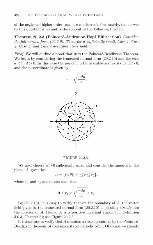
384 20. Bifurcation of Fixed Points of Vector Fields
of the neglected higher order term are considered? Fortunately, the answerto this question is no and is the content of the following theorem.
Theorem 20.2.3 (Poincare-Andronov-Hopf Bifurcation) Consider
the full normal form (20.2.9). Then, for µ sufficiently small, Case 1, Case
2, Case 3, and Case 4 described above hold.
Proof: We will outline a proof that uses the Poincare-Bendixson Theorem.We begin by considering the truncated normal form (20.2.10) and the casea < 0, d > 0. In this case the periodic orbit is stable and exists for µ > 0,and the r coordinate is given by
r =
√−dµ
a.
FIGURE 20.2.5.
We next choose µ > 0 sufficiently small and consider the annulus in theplane, A, given by
A = (r, θ)| r1 ≤ r ≤ r2 ,
where r1 and r2 are chosen such that
0 < r1 <
√−dµ
a< r2.
By (20.2.10), it is easy to verify that on the boundary of A, the vectorfield given by the truncated normal form (20.2.10) is pointing strictly intothe interior of A. Hence, A is a positive invariant region (cf. Definition3.0.3, Chapter 3); see Figure 20.2.5.
It is also easy to verify that A contains no fixed points so, by the Poincare-Bendixson theorem, A contains a stable periodic orbit. Of course we already
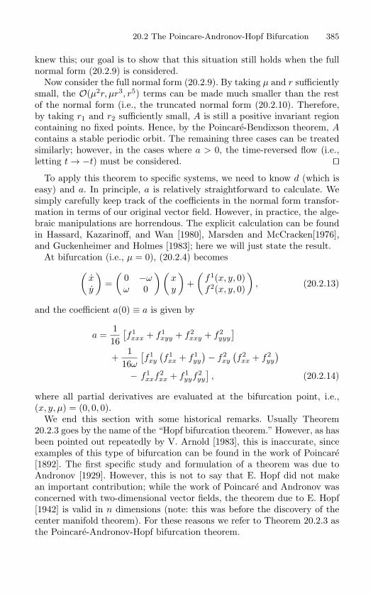
20.2 The Poincare-Andronov-Hopf Bifurcation 385
knew this; our goal is to show that this situation still holds when the fullnormal form (20.2.9) is considered.
Now consider the full normal form (20.2.9). By taking µ and r sufficientlysmall, the O(µ2r, µr3, r5) terms can be made much smaller than the restof the normal form (i.e., the truncated normal form (20.2.10). Therefore,by taking r1 and r2 sufficiently small, A is still a positive invariant regioncontaining no fixed points. Hence, by the Poincare-Bendixson theorem, Acontains a stable periodic orbit. The remaining three cases can be treatedsimilarly; however, in the cases where a > 0, the time-reversed flow (i.e.,letting t → −t) must be considered.
To apply this theorem to specific systems, we need to know d (which iseasy) and a. In principle, a is relatively straightforward to calculate. Wesimply carefully keep track of the coefficients in the normal form transfor-mation in terms of our original vector field. However, in practice, the alge-braic manipulations are horrendous. The explicit calculation can be foundin Hassard, Kazarinoff, and Wan [1980], Marsden and McCracken[1976],and Guckenheimer and Holmes [1983]; here we will just state the result.
At bifurcation (i.e., µ = 0), (20.2.4) becomes(xy
)=
(0 −ωω 0
)(xy
)+
(f1(x, y, 0)f2(x, y, 0)
), (20.2.13)
and the coefficient a(0) ≡ a is given by
a =116
[f1
xxx + f1xyy + f2
xxy + f2yyy
]+
116ω
[f1
xy
(f1
xx + f1yy
)− f2
xy
(f2
xx + f2yy
)− f1
xxf2xx + f1
yyf2yy
], (20.2.14)
where all partial derivatives are evaluated at the bifurcation point, i.e.,(x, y, µ) = (0, 0, 0).
We end this section with some historical remarks. Usually Theorem20.2.3 goes by the name of the “Hopf bifurcation theorem.” However, as hasbeen pointed out repeatedly by V. Arnold [1983], this is inaccurate, sinceexamples of this type of bifurcation can be found in the work of Poincare[1892]. The first specific study and formulation of a theorem was due toAndronov [1929]. However, this is not to say that E. Hopf did not makean important contribution; while the work of Poincare and Andronov wasconcerned with two-dimensional vector fields, the theorem due to E. Hopf[1942] is valid in n dimensions (note: this was before the discovery of thecenter manifold theorem). For these reasons we refer to Theorem 20.2.3 asthe Poincare-Andronov-Hopf bifurcation theorem.
386 20. Bifurcation of Fixed Points of Vector Fields
20.2a Exercises1. This exercise comes from Marsden and McCracken [1976]. Consider the following vector
fields
a) r = −r(r − µ)2,
θ = 1,(r, θ) ∈ R
+ × S1.
b) r = r(µ − r2)(2µ − r
2)2,
θ = 1.
c) r = r(r + µ)(r − µ),θ = 1.
d) r = µr(r2 − µ),θ = 1.
FIGURE 20.2.6.
e) r = −µ2r(r + µ)2(r − µ)2,
θ = 1.
20.3 Stability of Bifurcations Under Perturbations 387
Match each of these vector fields to the appropriate phase portrait in Figure 20.2.6 andexplain which hypotheses (if any) of the Poincare–Andronov–Hopf bifurcation theoremare violated.
2. Consider the Poincare–Andronov–Hopf bifurcation theorem (Theorem 20.2.3). Workout all of the details of the proof outlined that uses the Poincare–Bendixson theorem.
3. For the Poincare–Andronov–Hopf bifurcation, compute the expression for the coeffi-cient a given in (20.2.14).
20.3 Stability of Bifurcations Under Perturbations
Let us recall the central motivational question raised at the beginning ofthis chapter; namely, what is the nature of the orbit structure near a non-hyperbolic fixed point of a vector field? The key word to focus on in thisquestion is “near.” We have seen that a nonhyperbolic fixed point can beeither asymptotically stable or unstable. However, most importantly, wehave seen that “nearby vector fields” can have very different orbit struc-tures. The phrase “nearby vector fields” was made concrete by consideringparameterized families of vector fields; at a certain parameter value thefixed point was not hyperbolic, and a qualitatively different orbit structureexisted for nearby parameter values (i.e., new solutions were created as theparameter was varied). There is an important, general lesson to be learnedfrom this, which we state as follows.
Pure Mathematical Lesson
From the point of view of stability of nonhyperbolic fixed points of vectorfields, one should not only study the orbit structure near the fixed pointbut also the local orbit structure of nearby vector fields.
Applied Mathematical Lesson
From the point of view of “robustness” of mathematical models, supposeone has a vector field possessing a nonhyperbolic fixed point. The vectorfield should then possess enough (independent) parameters so that, as theparameters are varied, all possible local dynamical behavior is realized inthis particular parameterized family of vector fields.
Before making these somewhat vague ideas more precise, let us considerhow they are manifested in the saddle-node, transcritical, pitchfork, andPoincare-Andronov-Hopf bifurcations of vector fields that we have alreadystudied.
Example 20.3.1 (The Saddle-Node Bifurcation). Consider the one-parameter
family of one-dimensional vector fields
x = f(x, µ), y ∈ R1, µ ∈ R
1, (20.3.1)
with
f(0, 0) = 0, (20.3.2)
388 20. Bifurcation of Fixed Points of Vector Fields
∂f
∂x(0, 0) = 0. (20.3.3)
We saw in Section 20.1c that the conditions
∂f
∂µ(0, 0) = 0, (20.3.4)
∂2f
∂x2 (0, 0) = 0, (20.3.5)
were sufficient conditions in order for the vector field (20.3.1) to undergo a saddle-
node bifurcation at µ = 0. The question we ask is the following.
If a one-parameter family of one-dimensional vector fields satisfying
(20.3.2), (20.3.3), (20.3.4), and (20.3.5) is “perturbed,” will the re-
sulting family of one-dimensional vector fields have qualitatively the
same dynamics?
We will have essentially answered this question once we have explained what we
mean by the term “perturbed.”
We do this by first eliminating the parameters entirely. Consider a one-
dimensional vector field
x = f(x) = a0x2
+ O(x3), x ∈ R
1, (20.3.6)
where, in the Taylor expansion of f(x), we have omitted the constant and O(x)
terms, since we want (20.3.6) to have a nonhyperbolic fixed point at x = 0.
Because x = 0 is a nonhyperbolic fixed point, the orbit structure near x = 0 of
vector fields near (20.3.6) may be very different. We consider vector fields close
to (20.3.6) by embedding (20.3.6) in a one-parameter family of vector fields as
follows
x = f(x, µ) = µ + a0x2
+ O(x3). (20.3.7)
The addition of the term “µ” in (20.3.7) can be viewed as a perturbation of
(20.3.6) via adding lower-order terms in the Taylor expansion of the vector field
about the nonhyperbolic fixed point (note: “lower-order terms” means terms of
order lower than the first nonvanishing term in the Taylor expansion). Clearly,
(20.3.7) satisfies (20.3.2), (20.3.3), (20.3.4), and (20.3.5); hence, (x, µ) = (0, 0) is
a saddle-node bifurcation point. What about further perturbations of (20.3.7)?
If we add terms of O(x3) and larger, we see that this has no effect on the nature
of the bifurcation, since the saddle-node bifurcation is completely determined by
(20.3.2), (20.3.3), (20.3.4), and (20.3.5), i.e., by terms of O(x2) and lower. We
could perturb (20.3.7) further by adding lower-order terms. For example,
x = f(x, µ, ε) = µ + εx + a0x2
+ O(x3). (20.3.8)
In this case we have a two-parameter family of one-dimensional vector fields hav-
ing a nonhyperbolic fixed point at (x, µ, ε) = (0, 0, 0). However, the nature of the
saddle-node bifurcation (i.e., the geometry of the curve(s) of fixed points pass-
ing through the bifurcation point) is completely determined by (20.3.2), (20.3.3),
(20.3.4), and (20.3.5). Hence, the addition of the term “εx” in (20.3.8) does not
introduce any new dynamical phenomena into (20.3.7) (provided µ = 0).
End of Example 20.3.1
20.3 Stability of Bifurcations Under Perturbations 389
Example 20.3.2 (The Transcritical Bifurcation). Consider the one-parameter
family of one-dimensional vector fields
x = f(x, µ), x ∈ R1, µ ∈ R
1, (20.3.9)
with
f(0, 0) = 0, (20.3.10)
∂f
∂x(0, 0) = 0. (20.3.11)
We saw in Section 20.1d that if (20.3.9) also satisfies
∂f
∂µ(0, 0) = 0, (20.3.12)
∂2f
∂µ∂x(0, 0) = 0, (20.3.13)
∂2f
∂x2 (0, 0) = 0, (20.3.14)
then a transcritical bifurcation occurs at (x, µ) = (0, 0). The conditions (20.3.12),
(20.3.13), and (20.3.14) imply that, in the study of the orbit structure near the
bifurcation point, terms of O(x3) and larger in the Taylor expansion of the vector
field about the bifurcation point do not qualitatively affect the nature of the
bifurcation (i.e., they do not affect the geometry of the curves of fixed points
passing through the bifurcation point). From this we concluded that a normal
form for the transcritical bifurcation was given by
x = µx ∓ x2. (20.3.15)
Now let us consider a perturbation of the transcritical bifurcation by perturbing
this normal form. Following our discussion of the perturbation of the saddle-
node bifurcation and upon examining the defining conditions for the transcritical
bifurcation given in (20.3.12), (20.3.13), and (20.3.14), we see that the only way
to perturb (20.1.31) that may lead to qualitatively new dynamics is as follows
x = ε + µx ∓ x2. (20.3.16)
In Figure 20.3.1 we show what becomes of the transcritical bifurcation for
ε < 0, ε = 0, and ε > 0.
From this we see that the two curves of fixed points which pass through the
origin for ε = 0 break apart into either a pair of curves of fixed points on which
no bifurcation happens on passing through µ = 0 or a pair of saddle-node bifur-
cations.
End of Example 20.3.2
Example 20.3.3 (The Pitchfork Bifurcation). From (20.1.83), the normal form
for the pitchfork bifurcation was found to be
x = µx ∓ x3, x ∈ R1, µ ∈ R
1. (20.3.17)
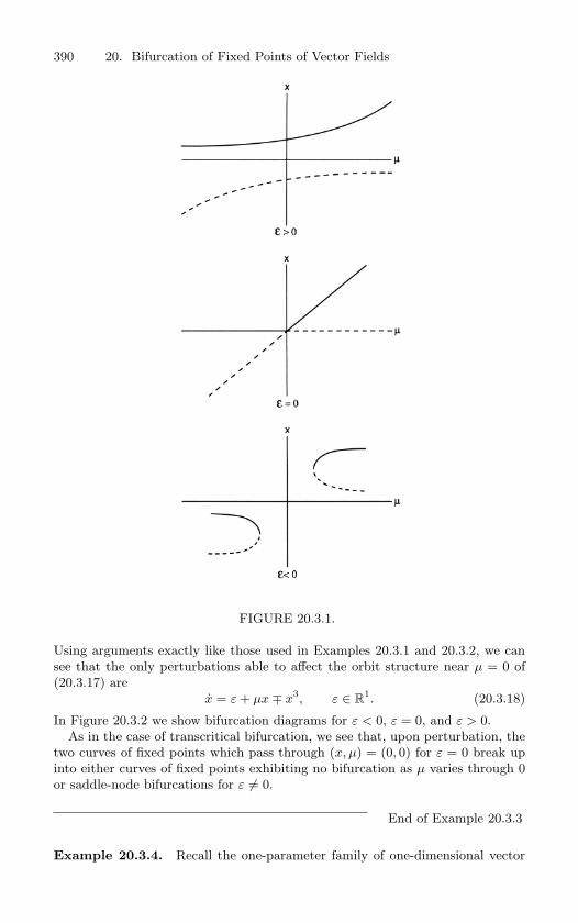
390 20. Bifurcation of Fixed Points of Vector Fields
FIGURE 20.3.1.
Using arguments exactly like those used in Examples 20.3.1 and 20.3.2, we can
see that the only perturbations able to affect the orbit structure near µ = 0 of
(20.3.17) are
x = ε + µx ∓ x3, ε ∈ R1. (20.3.18)
In Figure 20.3.2 we show bifurcation diagrams for ε < 0, ε = 0, and ε > 0.
As in the case of transcritical bifurcation, we see that, upon perturbation, the
two curves of fixed points which pass through (x, µ) = (0, 0) for ε = 0 break up
into either curves of fixed points exhibiting no bifurcation as µ varies through 0
or saddle-node bifurcations for ε = 0.
End of Example 20.3.3
Example 20.3.4. Recall the one-parameter family of one-dimensional vector
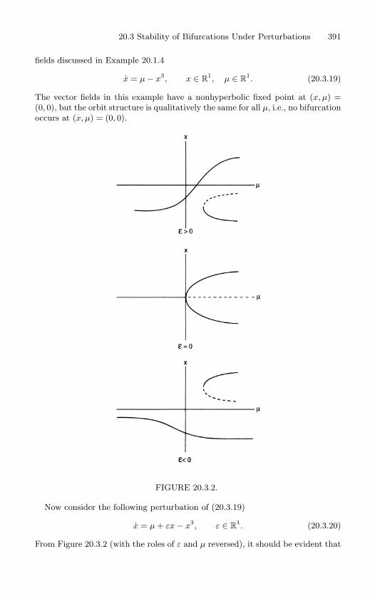
20.3 Stability of Bifurcations Under Perturbations 391
fields discussed in Example 20.1.4
x = µ − x3, x ∈ R1, µ ∈ R
1. (20.3.19)
The vector fields in this example have a nonhyperbolic fixed point at (x, µ) =
(0, 0), but the orbit structure is qualitatively the same for all µ, i.e., no bifurcation
occurs at (x, µ) = (0, 0).
FIGURE 20.3.2.
Now consider the following perturbation of (20.3.19)
x = µ + εx − x3, ε ∈ R1. (20.3.20)
From Figure 20.3.2 (with the roles of ε and µ reversed), it should be evident that
392 20. Bifurcation of Fixed Points of Vector Fields
(20.3.20) does exhibit saddle-node bifurcations for ε = 0.
End of Example 20.3.4
Example 20.3.5 (The Poincare-Andronov-Hopf Bifurcation). From Theorem
20.2.3, the normal form for the Poincare-Andronov-Hopf bifurcation was given
by
r = µdr + ar3, (r, θ) ∈ R+ × S1, µ ∈ R
1, (20.3.21)
θ = ω + cµ + br2. (20.3.22)
We want to consider how the bifurcation near (r, µ) = (0, 0) studied in Section
20.2 changes as (20.3.21) is perturbed. Three points should be considered.
1. Theorem 20.2.3 tells us that, for a = 0, d = 0, higher order terms (i.e.,
O(r4)) will not affect the dynamics of (20.3.21) near (r, µ) = (0, 0).
2. Since ω is a constant, for (r, µ) small, in order to determine the nature
of solutions bifurcating from the origin we need only worry about the rcomponent of the vector field (20.3.21).
3. Due to the structure of the linear part of the vector field, r = 0 is a fixed
point for µ sufficiently small and no terms of even order in r are present
in the r component of the normal form.
Using these three points, we see that, for a = 0, d = 0, no perturbations allowed
by the structure of the vector field (cf. the third point above) will qualitatively
alter the nature of the bifurcation near (r, µ) = (0, 0).
End of Example 20.3.5
From Examples 20.3.1–20.3.5 we might conclude that, in one-parameterfamilies of vector fields, the most “typical” bifurcations are saddle-nodeand Poincare-Andronov-Hopf. This is indeed the case, as we will show inSection 20.4. Moreover, these examples show that some nonhyperbolic fixedpoints are more degenerate than others in the sense that more parametersare needed in order to capture all possible nearby behavior. In Section 20.4we explore the idea of the codimension of a bifurcation, which will enableus to quantify these ideas. A complete theory is given by Golubitsky andSchaeffer [1985] and Golubitsky, Stewart, and Schaeffer [1988].
20.4 The Idea of the Codimension of a Bifurcation
We have seen that some types of bifurcations (e.g., transcritical, pitchfork)are more degenerate than others (e.g., saddle-node). In this section we willattempt to make this more precise by introducing the idea of the codimen-sion of a bifurcation. We will do this by starting with a heuristic discussion
20.4 The Idea of the Codimension of a Bifurcation 393
of the “big picture” of bifurcation theory. This will serve to show just howlittle is actually understood about bifurcation theory at this stage of themathematical development of nonlinear dynamical systems theory.
20.4a The “Big Picture” for Bifurcation TheoryThe first step is to eliminate the consideration of all parameters from theproblem; instead, we consider the infinite-dimensional space of all dynami-cal systems, either vector fields or maps. Within this space we consider thesubset of all structurally stable dynamical systems, which we denote as S.By the definition of structural stability (cf. Chapter 12), perturbations ofstructurally stable dynamical systems do not yield qualitatively new dy-namical phenomena. Thus, from the point of view of bifurcation theory, itis not dynamical systems in S that are of interest but rather dynamical sys-tems in the complement of S, denoted Sc, since perturbations of dynamicalsystems in Sc can result in systems exhibiting radically different dynamicalbehavior. Thus, in order to understand the types of bifurcations that mayoccur in a class of dynamical systems, it is necessary to understand thestructure of Sc.
Presumably, in order for a dynamical system to be in Sc, the system mustsatisfy a certain number of extra conditions or constraints. When viewedgeometrically in the infinite-dimensional function space setting, this can beinterpreted as implying that Sc is a lower-dimensional “surface” containedin the space of dynamical systems. Here we use the word “surface” in aheuristic sense. More specifically, it would be nice if we could show that Sc
is a codimension one submanifold. In practice, however, Sc may have sin-gular regions and therefore be more appropriately described as an algebraic
variety (see Arnold [1983]). In any case, for our heuristic discussion, it doesno harm for the reader to visualize Sc as a surface. Before proceeding withthis picture, let us first make a slight digression and define the notion ofthe “codimension of a submanifold.”
The Codimension of a Submanifold
Let M be an m-dimensional manifold and let N be an n-dimensional sub-manifold contained in M ; then the codimension of N is defined to be m−n.Equivalently, in a coordinate setting, the codimension of N is the numberof independent equations needed to define N . Thus, the codimension ofa submanifold is a measure of the avoidability of the submanifold as onemoves about the ambient space; in particular, the codimension of a sub-manifold N is equal to the minimum dimension of a submanifold P ⊂ Mthat intersects N such that the intersection is transversal. We have definedcodimension in a finite-dimensional setting, which permits some intuitionto be gained; now we move to the infinite-dimensional setting. Let M bean infinite-dimensional manifold and let N be a submanifold contained in
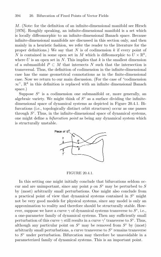
394 20. Bifurcation of Fixed Points of Vector Fields
M . (Note: for the definition of an infinite-dimensional manifold see Hirsch[1976]. Roughly speaking, an infinite-dimensional manifold is a set whichis locally diffeomorphic to an infinite-dimensional Banach space. Becauseinfinite-dimensional manifolds are discussed in this section only, and thenmainly in a heuristic fashion, we refer the reader to the literature for theproper definitions.) We say that N is of codimension k if every point ofN is contained in some open set in M which is diffeomorphic to U × R
k,where U is an open set in N . This implies that k is the smallest dimensionof a submanifold P ⊂ M that intersects N such that the intersection istransversal. Thus, the definition of codimension in the infinite-dimensionalcase has the same geometrical connotations as in the finite-dimensionalcase. Now we return to our main discussion. (For the case of “codimension∞”, R
k in this definition is replaced with an infinite dimensional Banachspace.)
Suppose Sc is a codimension one submanifold or, more generally, analgebraic variety. We might think of Sc as a surface dividing the infinite-dimensional space of dynamical systems as depicted in Figure 20.4.1. Bi-furcations (i.e., topologically distinct orbit structures) occur as one passesthrough Sc. Thus, in the infinite-dimensional space of dynamical systems,one might define a bifurcation point as being any dynamical system whichis structurally unstable.
FIGURE 20.4.1.
In this setting one might initially conclude that bifurcations seldom oc-cur and are unimportant, since any point p on Sc may be perturbed to Sby (most) arbitrarily small perturbations. One might also conclude froma practical point of view that dynamical systems contained in Sc mightnot be very good models for physical systems, since any model is only anapproximation to reality and therefore should be structurally stable. How-ever, suppose we have a curve γ of dynamical systems transverse to Sc, i.e.,a one-parameter family of dynamical systems. Then any sufficiently smallperturbation of this curve γ still results in a curve γ′ transverse to Sc. Thus,although any particular point on Sc may be removed from Sc by (most)arbitrarily small perturbations, a curve transverse to Sc remains transverseto Sc under perturbation. Bifurcation may therefore be unavoidable in aparameterized family of dynamical systems. This is an important point.
20.4 The Idea of the Codimension of a Bifurcation 395
Now, even if we are able to show that Sc is a codimension one submani-fold or algebraic variety, Sc itself may be divided up into objects of highercodimension corresponding to more degenerate types of bifurcations. A par-ticular type of codimension k bifurcation in Sc would then be persistent ina k-parameter family of dynamical systems transverse to the codimensionk submanifold.
This is essentially the program for bifurcation theory originally outlinedby Poincare. In order to utilize it in practice one would proceed as follows.
1. Given a specific dynamical system, determine whether or not it isstructurally stable.
2. If it is not structurally stable, compute the codimension of the bifur-cation.
3. Embed the system in a parameterized family of systems transverseto the bifurcation surface with the number of parameters equal tothe codimension of the bifurcation. These parameterized systems arecalled unfoldings or deformations and, if they contain all possiblequalitative dynamics that can occur near the bifurcation, they arecalled universal unfoldings or versal deformations; see Arnold [1983]and our discussion to follow.
4. Study the dynamics of the parametrized systems.
In this way one obtains structurally stable families of systems. More-over, this provides a method for gaining a complete understanding of thequalitative dynamics of the space of dynamical systems with as little workas possible; namely, one uses the degenerate bifurcation points as “orga-nizing centers” around which one studies the dynamics. Because elsewherethe dynamical systems are structurally stable, there is no need to worryabout the details of their dynamics; qualitatively, they will be topologicallyconjugate to the structurally stable dynamical systems in a neighborhoodof the bifurcation point.
This program is far from complete, and many of the problems associ-ated with its completion are exactly those encountered in our discussion ofstructural stability in Chapter 12. First, we must specify what we mean bythe “infinite-dimensional space of dynamical systems.” (Usually this doesnot present any major difficulties.) Next, we must equip the space with atopology in order to define what we mean by a perturbation of a dynamicalsystem. We have already seen (cf. Example 12.0.1 of Chapter 12) that therecan be problems with this if the phase space is unbounded; nevertheless,these difficulties can usually be brought under control. The real difficultyis the following. Given a dynamical system, what does one need to knowabout it in order to determine whether it is in S or Sc? For vector fields oncompact, boundaryless two-dimensional manifolds Peixoto’s theorem gives
396 20. Bifurcation of Fixed Points of Vector Fields
us an answer to this question (see Theorem 12.1.4 , Chapter 12), but, inhigher dimensions, we do not have nice analogs of this theorem. Moreover,the detailed structure of Sc is certainly beyond our reach at this time. Al-though the situation appears hopeless, some progress has been made alongtwo fronts:
1. Local bifurcations;
2. Global bifurcations of specific orbits.
Since the subject of this chapter is local bifurcations we will discuss onlythis aspect. In Chapter 33 we will see examples of global bifurcations; formore information see Wiggins [1988].
Local bifurcation theory is concerned with the bifurcation of fixed pointsof vector fields and maps or with situations in which the problem can becast into this form, such as in the study of bifurcations of periodic motions.For vector fields one can construct a local Poincare map (see Chapter 10)near the periodic orbit, thus reducing the problem to one of studying thebifurcation of a fixed point of a map, and for maps with a k periodic orbitone can consider the kth iterate of the map, thus reducing the problemto one of studying the bifurcation of a fixed point of the kth iterate ofthe map. Utilizing a procedure such as the center manifold theorem or theLyapunov-Schmidt reduction (see Chow and Hale [1982]), one can usuallyreduce the problem to that of studying an equation of the form
f(x, λ) = 0, (20.4.1)
where x ∈ Rn, λ ∈ R
p are the system parameters and f : Rn ×R
p → Rn is
assumed to be sufficiently smooth. The goal is to study the nature of thesolutions of (20.4.1) as λ varies. In particular, it would be interesting toknow for what parameter values solutions disappear or are created. Theseparticular parameters are called bifurcation values, and there exists an ex-tensive mathematical machinery called singularity theory (see Golubitskyand Guillemin [1973]) that deals with such questions. Singularity theory isconcerned with the local properties of smooth functions near a zero of thefunction. It provides a classification of the various cases based on codimen-sion in a spirit similar to that described in the beginning of the section.The reason this is possible is that the codimension k submanifolds in thespace of all smooth functions having zeroes can be described algebraicallyby imposing conditions on derivatives of the functions. This gives us away of classifying the various possible bifurcations and of computing theproper unfoldings or deformations. From this one might be led to believethat local bifurcation theory is a well-understood subject; however, this isnot the case. The problem arises in the study of degenerate local bifurca-tions, specifically, in codimension k (k ≥ 2) bifurcations of vector fields.Fundamental work of Takens [1974], Langford [1979], and Guckenheimer
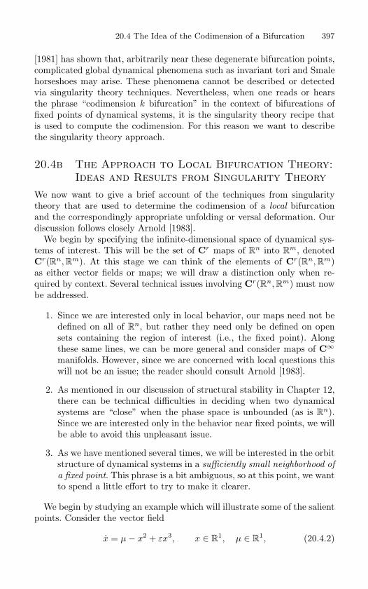
20.4 The Idea of the Codimension of a Bifurcation 397
[1981] has shown that, arbitrarily near these degenerate bifurcation points,complicated global dynamical phenomena such as invariant tori and Smalehorseshoes may arise. These phenomena cannot be described or detectedvia singularity theory techniques. Nevertheless, when one reads or hearsthe phrase “codimension k bifurcation” in the context of bifurcations offixed points of dynamical systems, it is the singularity theory recipe thatis used to compute the codimension. For this reason we want to describethe singularity theory approach.
20.4b The Approach to Local Bifurcation Theory:Ideas and Results from Singularity Theory
We now want to give a brief account of the techniques from singularitytheory that are used to determine the codimension of a local bifurcationand the correspondingly appropriate unfolding or versal deformation. Ourdiscussion follows closely Arnold [1983].
We begin by specifying the infinite-dimensional space of dynamical sys-tems of interest. This will be the set of Cr maps of R
n into Rm, denoted
Cr(Rn, Rm). At this stage we can think of the elements of Cr(Rn, Rm)as either vector fields or maps; we will draw a distinction only when re-quired by context. Several technical issues involving Cr(Rn, Rm) must nowbe addressed.
1. Since we are interested only in local behavior, our maps need not bedefined on all of R
n, but rather they need only be defined on opensets containing the region of interest (i.e., the fixed point). Alongthese same lines, we can be more general and consider maps of C∞
manifolds. However, since we are concerned with local questions thiswill not be an issue; the reader should consult Arnold [1983].
2. As mentioned in our discussion of structural stability in Chapter 12,there can be technical difficulties in deciding when two dynamicalsystems are “close” when the phase space is unbounded (as is R
n).Since we are interested only in the behavior near fixed points, we willbe able to avoid this unpleasant issue.
3. As we have mentioned several times, we will be interested in the orbitstructure of dynamical systems in a sufficiently small neighborhood of
a fixed point. This phrase is a bit ambiguous, so at this point, we wantto spend a little effort to try to make it clearer.
We begin by studying an example which will illustrate some of the salientpoints. Consider the vector field
x = µ− x2 + εx3, x ∈ R1, µ ∈ R
1, (20.4.2)
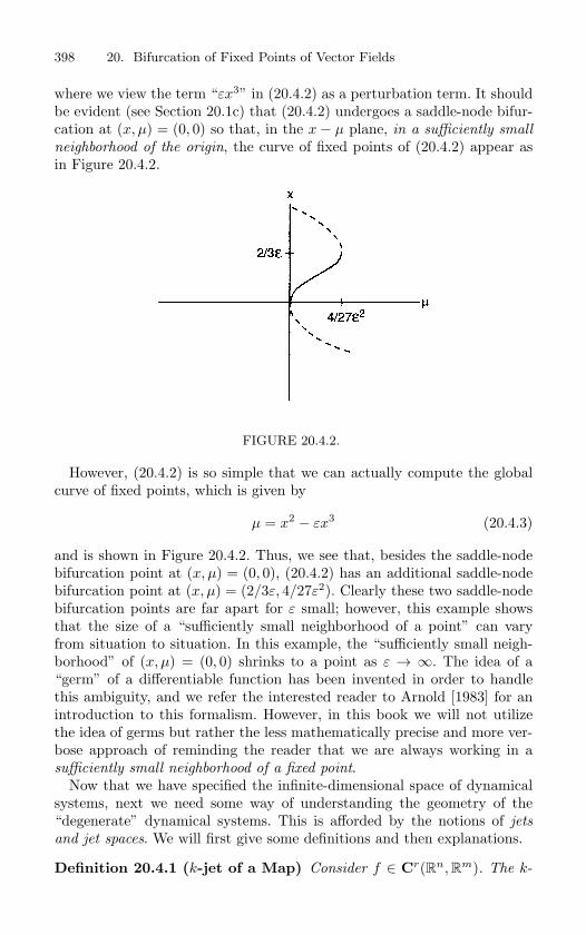
398 20. Bifurcation of Fixed Points of Vector Fields
where we view the term “εx3” in (20.4.2) as a perturbation term. It shouldbe evident (see Section 20.1c) that (20.4.2) undergoes a saddle-node bifur-cation at (x, µ) = (0, 0) so that, in the x− µ plane, in a sufficiently small
neighborhood of the origin, the curve of fixed points of (20.4.2) appear asin Figure 20.4.2.
FIGURE 20.4.2.
However, (20.4.2) is so simple that we can actually compute the globalcurve of fixed points, which is given by
µ = x2 − εx3 (20.4.3)
and is shown in Figure 20.4.2. Thus, we see that, besides the saddle-nodebifurcation point at (x, µ) = (0, 0), (20.4.2) has an additional saddle-nodebifurcation point at (x, µ) = (2/3ε, 4/27ε2). Clearly these two saddle-nodebifurcation points are far apart for ε small; however, this example showsthat the size of a “sufficiently small neighborhood of a point” can varyfrom situation to situation. In this example, the “sufficiently small neigh-borhood” of (x, µ) = (0, 0) shrinks to a point as ε → ∞. The idea of a“germ” of a differentiable function has been invented in order to handlethis ambiguity, and we refer the interested reader to Arnold [1983] for anintroduction to this formalism. However, in this book we will not utilizethe idea of germs but rather the less mathematically precise and more ver-bose approach of reminding the reader that we are always working in asufficiently small neighborhood of a fixed point.
Now that we have specified the infinite-dimensional space of dynamicalsystems, next we need some way of understanding the geometry of the“degenerate” dynamical systems. This is afforded by the notions of jets
and jet spaces. We will first give some definitions and then explanations.
Definition 20.4.1 (k-jet of a Map) Consider f ∈ Cr(Rn, Rm). The k-
20.4 The Idea of the Codimension of a Bifurcation 399
jet of f at x (k ≤ r) is given by the following (k + 2)-tuple
(x, f(x), Df(x), · · · , Dkf(x)).
Thus we see that the k-jet of a map at a point is simply the Taylorcoefficients through order k plus the point at which they are evaluated. Wedenote the k-jet of f at x by
Jkx (f).
Although it may seem a bit silly to dress up something as commonplace asa Taylor expansion in a new formalism, the reader will see that there is adefinite payoff. We next consider the set of all k-jets of Cr (k ≤ r) maps ofR
n into Rm at all points of R
n.
Definition 20.4.2 (The Space of k-jets) The set of all k-jets of Cr
(k ≤ r) maps of Rn into R
m at all points of Rn is called the space of
k-jets and is denoted by
Jk(Rn, Rm) = The space of k-jets ofC∞maps ofRnintoRm .
The spaces Jk(Rn, Rm) have a nice linear vector space structure. In fact,we can identify Jk(Rn, Rm) with R
p for an appropriate choice of p. Weillustrate this in the following examples.
Example 20.4.1. J0(Rn, Rm) = Rn × Rm.
End of Example 20.4.1
Example 20.4.2. J1(R1, R1) is three dimensional, because points in J1(R1, R1)
can be assigned the coordinates(x, f(x),
∂f
∂x(x)
).
End of Example 20.4.2
Example 20.4.3. J1(R2, R2) is eight dimensional, because points in J1(R2, R2)
can be assigned the coordinates
(x, f(x), Df(x)),
where Df(x) is a 2 × 2 matrix.
End of Example 20.4.3
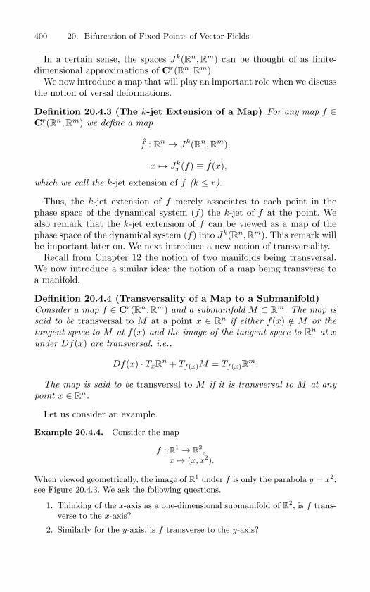
400 20. Bifurcation of Fixed Points of Vector Fields
In a certain sense, the spaces Jk(Rn, Rm) can be thought of as finite-dimensional approximations of Cr(Rn, Rm).
We now introduce a map that will play an important role when we discussthe notion of versal deformations.
Definition 20.4.3 (The k-jet Extension of a Map) For any map f ∈Cr(Rn, Rm) we define a map
f : Rn → Jk(Rn, Rm),
x → Jkx (f) ≡ f(x),
which we call the k-jet extension of f (k ≤ r).
Thus, the k-jet extension of f merely associates to each point in thephase space of the dynamical system (f) the k-jet of f at the point. Wealso remark that the k-jet extension of f can be viewed as a map of thephase space of the dynamical system (f) into Jk(Rn, Rm). This remark willbe important later on. We next introduce a new notion of transversality.
Recall from Chapter 12 the notion of two manifolds being transversal.We now introduce a similar idea: the notion of a map being transverse toa manifold.
Definition 20.4.4 (Transversality of a Map to a Submanifold)Consider a map f ∈ Cr(Rn, Rm) and a submanifold M ⊂ R
m. The map is
said to be transversal to M at a point x ∈ Rn if either f(x) /∈ M or the
tangent space to M at f(x) and the image of the tangent space to Rn at x
under Df(x) are transversal, i.e.,
Df(x) · TxRn + Tf(x)M = Tf(x)R
m.
The map is said to be transversal to M if it is transversal to M at any
point x ∈ Rn.
Let us consider an example.
Example 20.4.4. Consider the map
f : R1 → R2,x → (x, x2).
When viewed geometrically, the image of R1 under f is only the parabola y = x2;
see Figure 20.4.3. We ask the following questions.
1. Thinking of the x-axis as a one-dimensional submanifold of R2, is f trans-
verse to the x-axis?
2. Similarly for the y-axis, is f transverse to the y-axis?
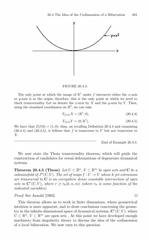
20.4 The Idea of the Codimension of a Bifurcation 401
FIGURE 20.4.3.
The only point at which the image of R1 under f intersects either the x-axis
or y-axis is at the origin; therefore, this is the only point at which we need to
check transversality. Let us denote the x-axis by X and the y-axis by Y . Then,
using the standard coordinates on R2, we can take
T(0,0)X = (R1, 0), (20.4.4)
T(0,0)Y = (0, R1). (20.4.5)
We have that Df(0) = (1, 0); thus, on recalling Definition 20.4.4 and examining
(20.4.4) and (20.4.5), it follows that f is transverse to Y but not transverse to
X.
End of Example 20.4.4
We now state the Thom transversality theorem, which will guide theconstruction of candidates for versal deformations of degenerate dynamicalsystems.
Theorem 20.4.5 (Thom) Let U ⊂ Rn, V ⊂ R
m be open sets and C be a
submanifold of Jk(U, V ). The set of maps f : U → V whose k-jet extensions
are transversal to C is an everywhere dense countable intersection of open
sets in Cr(U, V ), where r ≥ r0(k, n, m) (where r0 is some function of the
indicated variables).
Proof: See Arnold [1983]. This theorem allows us to work in finite dimensions, where geometrical
intuition is more apparent, and to draw conclusions concerning the geome-try in the infinite-dimensional space of dynamical systems, Cr(U, V ), whereU ⊂ R
n, V ⊂ Rm are open sets . At this point we have developed enough
machinery from singularity theory to discuss the idea of the codimensionof a local bifurcation. We now turn to this question.
402 20. Bifurcation of Fixed Points of Vector Fields
20.4c The Codimension of a Local BifurcationAs mentioned in our discussion of the “big picture” of bifurcation theory,the problem we are immediately faced with is determining whether a dy-namical system is structurally stable. If we limit ourselves to the study ofthe behavior of fixed points, then the problem is much easier, because weknow how to characterize structurally unstable fixed points—they are sim-ply the nonhyperbolic fixed points. The techniques from singularity theorywe developed in 20.4 will enable us to characterize the degree of “structuralinstability” of a fixed point in a way that is similar in spirit to our discussionof the “big picture” of bifurcation theory given in that section. However,the reader should realize that these ideas are concerned with fixed pointbehavior only and as such we must often do additional work to determinewhether nearby dynamical phenomena are properly taken into account. Wewill see several examples of this as we go along.
Thus far we have been using the term “dynamical system” to refer tovector fields and maps interchangeably. At this stage we need to drawa slight distinction. We will be studying the fixed points of dynamicalsystems. For vector fields
x = f(x), x ∈ Rn, (20.4.6)
this means studying the equation
f(x) = 0, (20.4.7)
and for mapsx → g(x), x ∈ R
n, (20.4.8)
this means studying the equation
g(x)− x = 0. (20.4.9)
It should be clear that from an analytic point of view, (20.4.7) and (20.4.9)are essentially the same. However, for the remainder of this section we willdeal solely with vector fields and leave the trivial modifications for mapsas exercises.
For vector fields the space of dynamical systems will be Cr(U, V ) andthe associated jet spaces Jk(U, V ), where U ⊂ R
n, V ⊂ Rm are open sets.
In particular, we will work solely in the finite-dimensional space Jk(U, V ).Within Jk(U, V ) we will be interested in the subset consisting of k-jets ofvector fields having fixed points. We denote this subset by F (for fixedpoints) and note that F has codimension n. Within F we will be interestedin the k-jets of vector fields having nonhyperbolic fixed points. We denotethis subset by B (for bifurcation) and note the B has codimension n + 1.We remark that the codimension of F and B is independent of k; however,the dimension of F and B is not independent of k. Let us now considersome specific examples.
20.4 The Idea of the Codimension of a Bifurcation 403
Example 20.4.5 (One-Dimensional Vector Fields). As our space of vector fields
we take Cr(R1, R1). In this case Jk(R1, R1) is (k+2)-dimensional with coordinates
of points in Jk(Rn, Rn) given by the (k + 2)-tuples(x, f(x),
∂f
∂x(x),
∂2f
∂x2 (x), · · · , ∂kf
∂xk(x)
), x ∈ R
1, f ∈ Cr(R
1, R1),
F is (k + 1)-dimensional (codimension 1) with coordinates of points in F given
by (x, 0,
∂f
∂x(x),
∂2f
∂x2 (x), · · · , ∂kf
∂xk(x)
), x ∈ R
1, f ∈ Cr(R
1, R1),
and B is k-dimensional (codimension 2) with coordinates of points in B given by(x, 0, 0,
∂2f
∂x2 (x), · · · , ∂kf
∂xk(x)
), x ∈ R
1, f ∈ Cr(R
1, R1).
End of Example 20.4.5
Example 20.4.6 (n-Dimensional Vector Fields). As our space of vector fields
we take Cr(Rn, Rn). In this case coordinates of Jk(Rn, Rn) are given by(x, f(x), Df(x), · · · , Dkf(x)
), x ∈ R
n, f ∈ Cr(R
n, Rn).
F is codimension n, with points in F having coordinates(x, 0, Df(x), · · · , Dkf(x)
), x ∈ R
n, f ∈ Cr(R
n, Rn),
and B is codimension n + 1, with points in B having coordinates(x, 0, Df(x), · · · , Dkf(x)
), x ∈ R
n, f ∈ Cr(R
n, Rn),
where Df(x) represents a nonhyperbolic matrix which lies on a surface of codi-
mension 1 in the n2-dimensional space of n × n matrices. This is explained in
great detail in Section 20.5.
End of Example 20.4.6
We are now at the point where we can define the codimension of a fixed
point. There are two possibilities for the choice of this number, and weclosely follow the discussion of Arnold [1972].
Definition 20.4.6 (The Codimension of a Fixed Point) Consider Jk
(Rn, Rn) and the subset of Jk(Rn, Rn) consisting of k-jets of elements of
Cr(Rn, Rn) that have fixed points. We denote this subset by F and note
that F has codimension n in Jk(Rn, Rn). Consider the k-jet of an element
of Cr(Rn, Rn) that has a nonhyperbolic fixed point. Then this k-jet lies in
a subset of F defined by conditions on the derivatives. Suppose this subset
of F has codimension b in Jk(Rn, Rn). Then we define the codimension of
the fixed point to be b− n.
404 20. Bifurcation of Fixed Points of Vector Fields
Before giving examples we want to make a few general remarks concern-ing this definition.
Remark 1. Evidently k must be taken sufficiently large so that the degreeof degeneracy of the nonhyperbolic fixed point can be specified.
Remark 2. This definition says that the codimension of a fixed point is equalto the codimension of the subset of F specified by the degeneracy of thefixed point minus n. Thus, hyperbolic fixed points have codimension zero bythis definition. This seems reasonable, since the notion of the codimensionof a fixed point should somehow specify the degree of “nongenericity” ofthe fixed point.
Remark 3. There is another way of describing the reasons why we chose thisway of defining the codimension of a fixed point. The dynamical system in-duces a map of the phase space, R
n, into Jk(Rn, Rn). This map is only thek-jet extension map (cf. Definition 20.4.3). At hyperbolic fixed points thismap is transverse to the subset F of Jk(Rn, Rn). Thus, hyperbolic fixedpoints cannot be destroyed by small perturbations. Hence, if the notion ofcodimension is to quantify the amount of “degeneracy” of nonhyperbolicfixed points, then the generic elements of F should be regarded as codi-mension zero. Practically speaking, this also implies that generically thefixed points move if they are perturbed.
Now we consider several examples where we will compute the codimen-sion.
Example 20.4.7. Consider the vector field
x = f(x) = ax2+ O(x3
), x ∈ R1. (20.4.10)
We are interested in studying (20.4.10) near the nonhyperbolic fixed point x = 0.
At this point we see that the k-jet of (20.4.10) is a typical element of the set
B described in Example 20.4.5. Hence, using Definition 20.4.6, we conclude that
x = 0 is codimension 1.
End of Example 20.4.7
Example 20.4.8. Consider the vector field
x = f(x) = ax3+ O(x4
), x ∈ R1. (20.4.11)
We are interested in (20.4.11) near the nonhyperbolic fixed point x = 0. As
in Example 20.4.7, the k-jet of (20.4.11) is contained in the set B described in
Example 20.4.5. However, (20.4.11) is more degenerate than the typical element
of B in that (20.4.11) also has
∂2f
∂x2 (0) = 0.
20.4 The Idea of the Codimension of a Bifurcation 405
Hence, the k-jet of (20.4.11) lies in a lower dimensional subset of B, denoted B′,which has codimension 3 in Jk(R1, R1), with points in B′ having coordinates(
x, 0, 0, 0,∂3f
∂x2 (x), · · · , ∂kf
∂xk(x)
), x ∈ R
n, f ∈ Cr(R
n, Rn).
Using Definition 20.4.6 we can thus conclude that x = 0 is codimension 2.
End of Example 20.4.8
Example 20.4.9. In Section 20.5 we show the following.
1. In the four-dimensional space of 2 × 2 real matrices the matrices(0 −ωω 0
)(20.4.12)
and (0 1
0 0
)(20.4.13)
lie on surfaces of codimension 2.
2. In the nine-dimensional space of 3 × 3 real matrices the matrix 0 −ω 0
ω 0 0
0 0 0
(20.4.14)
lies on a surface of codimension 3.
Hence, using Example 20.4.6 and Definition 20.4.6, we might conclude that the
codimension of a fixed point of a vector field whose 1-jet in (real) Jordan canonical
form is given by (20.4.12), (20.4.13), or (20.4.14) is 2, 2, and 3, respectively.
However, this is not quite true. By a re-parametrization of time, we can show
that cases (20.4.12), and (20.4.14) are codimension 1 and 2, respectively. This
is another way in which dynamics enters to slightly cloud the singularity theory
approach to classifying the degeneracy of an equilibrium point of a vector field.
End of Example 20.4.9
We end this section with two remarks.
Remark 1. The codimensions computed in these examples are for genericvector fields. In particular, we have not considered the possibility of symme-tries which would put extra constraints on eigenvalues and of derivativeswhich would result in a modification of the codimension; see Golubitskyand Schaeffer [1985] and Golubitsky, Stewart, and Schaeffer [1988].
Remark 2. We have referred to the sets F and B as “subsets” of Jk(Rn, Rn).In applying the Thom transversality theorem the question of whether ornot they are actually submanifolds arises. The same question is also ofinterest for the higher codimension subsets of B corresponding to more
406 20. Bifurcation of Fixed Points of Vector Fields
degenerate fixed points. In general, these subsets may have singular pointsand, thus, they will not have the structure of a submanifold. However,these singularities can be removed by slight perturbations and, hence, forour purposes, they can be treated as submanifolds. This technical point istreated in great detail in Gibson [1979].
20.4d Construction of Versal DeformationsWe now want to develop the necessary definitions in order to discuss versal
deformations of vector fields. We follow Arnold [1972], [1983] very closely.We remark the the phrase “unfolding” is often used to refer to a simi-lar procedure; see, e.g., Guckenheimer and Holmes [1983] (where the term“universal unfolding” is taken to be virtually synonymous with the phrase“versal deformation”) or Golubitsky and Schaeffer [1985] (where varioussubtleties in the definitions are thoroughly explored).
Consider the following Cr, parameter-dependent vector fields
x = f(x, λ), x ∈ Rn, λ ∈ R
, (20.4.15)
y = g(y, λ), y ∈ Rn, λ ∈ R
. (20.4.16)
We will be concerned with local behavior of these vector fields near fixedpoints. Therefore, we assume that (20.4.15) and (20.4.16) have fixed pointsat (x0, λ0) and (y0, λ0), respectively, and we will be concerned with thedynamics in a sufficiently small neighborhood of these points. We now givea parametric version of the notion of C0-equivalence given in Definition19.12.1.
Definition 20.4.7 (Parametric Version of C0-Equivalence) Equa-
tions (20.4.15) and (20.4.16) are said to be C0-equivalent (or topologically
equivalent) if there exists a continuous map
h : U → V,
with U a neighborhood of (x0, λ0) and V a neighborhood of y0 such that,
for λ sufficiently close to λ0,
h(·, λ),
with h(x0, λ0) = y0, is a homeomorphism that takes orbits of the flow gener-
ated by (20.4.15) onto orbits of the flow generated by (20.4.16), preserving
orientation but not necessarily parameterization by time. If h does preserve
parameterization by time, then (20.4.15) and (20.4.16) are said to be C0
conjugate (or topologically conjugate).
In the construction of versal deformations we will be concerned withhaving the minimum number of parameters (for reasons to be discussedlater), not too many or too few. The following definition is the first steptoward formalizing this notion.
20.4 The Idea of the Codimension of a Bifurcation 407
Consider the following Cr vector field
x = u(x, µ), x ∈ Rn, µ ∈ R
m, (20.4.17)
withu(x0, µ0) = 0.
Then we have the following definition.
Definition 20.4.8 (Family Induced from a Deformation) Let λ =φ(µ) be a continuous map defined for µ sufficiently close to µ0 with λ0 =φ(µ0). We say that (20.4.17) is induced from (20.4.15) if
u(x, µ) = f(x, φ(µ)).
We now can give our main definition.
Definition 20.4.9 (Versal Deformation) Equation (20.4.15) is called
a C0-equivalent versal deformation (or just versal deformation) of
x = f(x, λ0) (20.4.18)
at the point x0 if every other parameterized family of Cr vector fields that
reduces to (20.4.18) for a particular choice of parameters is equivalent to
a family of vector fields induced from (20.4.15).
At this point we again remind the reader that we are working in a suf-
ficiently small neighborhood of (x0, λ0). We are now at the stage where wecan construct versal deformations of dynamical systems. We will deal withvector fields and merely state the simple modifications needed for dealingwith maps.
Once we have a vector field having a nonhyperbolic fixed point there arefour steps necessary in order to construct a versal deformation.
Steps in the Construction of a Versal Deformation
Step 1. Put the vector field in normal form to reduce the number of casesthat need to be considered.
Step 2. Truncate the normal form and embed the resulting k-jet of thenormal form in a parameterized family having the number of pa-rameters equal to the codimension of the bifurcation such that theparameterized family of k-jets is transverse to the appropriate subsetof degenerate k-jets.
Step 3. Appeal to the Thom transversality theorem (Theorem 20.4.5) toargue that in this way one has constructed a generic family. By theterm generic family we mean a family from an everywhere dense setin the space of all families.
408 20. Bifurcation of Fixed Points of Vector Fields
Step 4. Prove that the parametrized family constructed in this manner isactually a versal deformation.
It should be apparent that Step 4 is by far the most difficult. Steps 1through 3 merely give us a procedure for constructing a parameterizedfamily that we hope will be a versal deformation. The reason why it maynot be is related to dynamics. The whole procedure is static only in nature;it takes into account only the nature of the fixed point. For one-dimensionalvector fields we will see that the method will yield versal deformations, sincethe only possible orbits distinguished by C0 equivalence are fixed points.However, for higher dimensional vector fields we will see that the methodmay not yield versal deformations and, indeed, no such versal deformationmay exist.
Elimination of a Parameter in One-Dimensional Vector Fields. Before
constructing candidates for versal deformations of vector fields we men-
tion a technical point relevant to one dimensional vector fields that
enables us to eliminate a parameter in some circumstances. Consider an
n-parameter family of one-dimensional vector fields of the form
f(x, µ) = µ1 + µ2x + µ3x2
+ · · · + µnxn−1 ± axn, (20.4.19)
where
x ∈ R1, a = 0, µ ≡ (µ1, . . . , µn) ∈ R
n.
Let us suppose that we make the following coordinate shift:
x → x + c,
with c to be chosen shortly. Then (20.4.19) can be rewritten as
f(x, µ) = µ1 + µ2(x + c) + µ3(x2
+ 2cx + c2)
+ · · · + µn(cn−1+ (n − 1)cn−2x + · · · + xn−1
)
± a(cn+ ncn−1x + · · · + ncxn−1
+ xn), (20.4.20)
where the coefficients multiplying each µi can be computed using the
binomial formula. The terms can then be rearranged, yielding a poly-
nomial in x of degree n. It is easy to see that after this is done the
coefficient multiplying xn−1 is given by
µn ± anc.
Then if we choose
c = ∓µn
an,
the xn−1 term does not appear.
Hence, we have shown that given an n-parameter family of one-
dimensional vector fields of the form
f(x, µ) = µ1 + µ2x + µ3x2
+ · · · + µnxn−1 ± axn, (20.4.21)
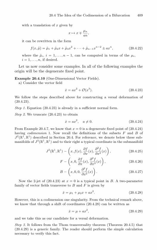
20.4 The Idea of the Codimension of a Bifurcation 409
with a translation of x given by
x → x ∓ µn
an,
it can be rewritten in the form
f(x, µ) = µ1 + µ2x + µ3x2
+ · · · + µn−1xn−2 ± axn, (20.4.22)
where the µi, i = 1, . . . , n − 1, can be computed in terms of the µi,
i = 1, . . . , n, if desired.
Let us now consider some examples. In all of the following examples theorigin will be the degenerate fixed point.
Example 20.4.10 (One-Dimensional Vector Fields).
a) Consider the vector field
x = ax2+ O(x3
). (20.4.23)
We follow the steps described above for constructing a versal deformation of
(20.4.23).
Step 1. Equation (20.4.23) is already in a sufficient normal form.
Step 2. We truncate (20.4.23) to obtain
x = ax2, a = 0. (20.4.24)
From Example 20.4.7, we know that x = 0 is a degenerate fixed point of (20.4.24)
having codimension 1. Now recall the definitions of the subsets F and B of
J2(R1, R1) described in Section 20.4. For reference, we denote below these sub-
manifolds of J2(R1, R1) and to their right a typical coordinate in the submanifold
J2(R
1, R1) −
(x, f(x),
∂f
∂x(x),
∂2f
∂x2 (x)
), (20.4.25)
F −(
x, 0,∂f
∂x(x),
∂2f
∂x2 (x)
), (20.4.26)
B −(
x, 0, 0,∂2f
∂x2 (x)
). (20.4.27)
Now the 2-jet of (20.4.23) at x = 0 is a typical point in B. A two-parameter
family of vector fields transverse to B and F is given by
x = µ1 + µ2x + ax2. (20.4.28)
However, this is a codimension one singularity. From the technical remark above,
we know that through a shift of coordinates (20.4.28) can be written as
x = µ + ax2, (20.4.29)
and we take this as our candidate for a versal deformation.
Step 3. It follows from the Thom transversality theorem (Theorem 20.4.5) that
(20.4.29) is a generic family. The reader should perform the simple calculation
necessary to verify this fact.
410 20. Bifurcation of Fixed Points of Vector Fields
Step 4. In Section 20.1c we showed that higher order terms do not affect the
dynamics of (20.4.29) near (x, µ) = (0, 0). Hence, the deformation is versal.
We can conclude from this that the saddle-node bifurcation is generic in one-
parameter families of vector fields.
b) Consider the vector field
x = ax3+ O(x4
). (20.4.30)
Step 1. Equation (20.4.30) is already in a sufficient normal form.
Step 2. We truncate (20.4.30) to obtain
x = ax3. (20.4.31)
From Example 20.4.8, x = 0 is a codimension 2 fixed point. For reference, we
denote below the subsets B′, B, and F of J3(R1, R1) discussed in Example 20.4.8
with typical coordinates immediately to the right.
J3(R
1, R1) −
(x, f(x),
∂f
∂x(x),
∂2f
∂x2 (x),∂3f
∂x3 (x)
), (20.4.32)
F −(
x, 0,∂f
∂x(x),
∂2f
∂x2 (x),∂3f
∂x3 (x)
), (20.4.33)
B −(
x, 0, 0,∂2f
∂x2 (x),∂3f
∂x3 (x)
), (20.4.34)
B′ −(
x, 0, 0, 0,∂3f
∂x3 (x)
). (20.4.35)
Since this is a codimension two singularity we want to embed (20.4.31) in a
two-parameter generic family transverse. Following the same reasoning given in
the previous example, we obtain
x = µ1 + µ2x + ax3, (20.4.36)
as a candidate for a versal deformation.
Step 3. It is an immediate consequence of the Thom transversality theorem (The-
orem 20.4.5) that (20.4.36) is a generic family. The reader should perform the
calculations necessary to verify this statement.
Step 4. In Section 20.1e, we proved that higher order terms do not qualitatively
effect the local dynamics of (20.4.36). Hence, we have found a versal deformation
of (20.4.30).
End of Example 20.4.10
Example 20.4.11 (Two-Dimensional Vector Fields).
a) The Poincare-Andronov-Hopf Bifurcation
Consider the vector field
x = −ωy + O(2),
y = ωx + O(2). (20.4.37)
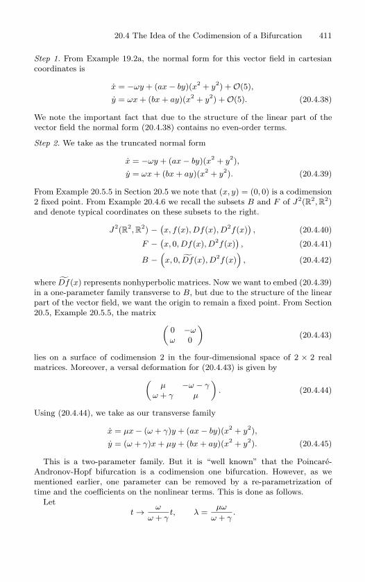
20.4 The Idea of the Codimension of a Bifurcation 411
Step 1. From Example 19.2a, the normal form for this vector field in cartesian
coordinates is
x = −ωy + (ax − by)(x2+ y2
) + O(5),
y = ωx + (bx + ay)(x2+ y2
) + O(5). (20.4.38)
We note the important fact that due to the structure of the linear part of the
vector field the normal form (20.4.38) contains no even-order terms.
Step 2. We take as the truncated normal form
x = −ωy + (ax − by)(x2+ y2
),
y = ωx + (bx + ay)(x2+ y2
). (20.4.39)
From Example 20.5.5 in Section 20.5 we note that (x, y) = (0, 0) is a codimension
2 fixed point. From Example 20.4.6 we recall the subsets B and F of J2(R2, R2)
and denote typical coordinates on these subsets to the right.
J2(R
2, R2) − (
x, f(x), Df(x), D2f(x)), (20.4.40)
F − (x, 0, Df(x), D2f(x)
), (20.4.41)
B −(x, 0, Df(x), D2f(x)
), (20.4.42)
where Df(x) represents nonhyperbolic matrices. Now we want to embed (20.4.39)
in a one-parameter family transverse to B, but due to the structure of the linear
part of the vector field, we want the origin to remain a fixed point. From Section
20.5, Example 20.5.5, the matrix (0 −ωω 0
)(20.4.43)
lies on a surface of codimension 2 in the four-dimensional space of 2 × 2 real
matrices. Moreover, a versal deformation for (20.4.43) is given by(µ −ω − γ
ω + γ µ
). (20.4.44)
Using (20.4.44), we take as our transverse family
x = µx − (ω + γ)y + (ax − by)(x2+ y2
),
y = (ω + γ)x + µy + (bx + ay)(x2+ y2
). (20.4.45)
This is a two-parameter family. But it is “well known” that the Poincare-
Andronov-Hopf bifurcation is a codimension one bifurcation. However, as we
mentioned earlier, one parameter can be removed by a re-parametrization of
time and the coefficients on the nonlinear terms. This is done as follows.
Let
t → ω
ω + γt, λ =
µω
ω + γ.
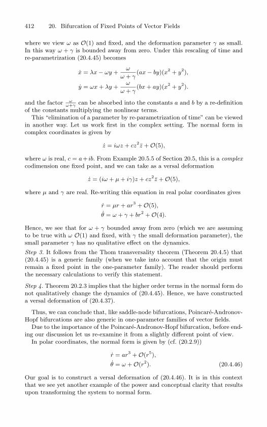
412 20. Bifurcation of Fixed Points of Vector Fields
where we view ω as O(1) and fixed, and the deformation parameter γ as small.
In this way ω + γ is bounded away from zero. Under this rescaling of time and
re-parametrization (20.4.45) becomes
x = λx − ωy +ω
ω + γ(ax − by)(x2
+ y2),
y = ωx + λy +ω
ω + γ(bx + ay)(x2
+ y2).
and the factor ωω+γ
can be absorbed into the constants a and b by a re-definition
of the constants multiplying the nonlinear terms.
This “elimination of a parameter by re-parametrization of time” can be viewed
in another way. Let us work first in the complex setting. The normal form in
complex coordinates is given by
z = iωz + cz2z + O(5),
where ω is real, c = a+ ib. From Example 20.5.5 of Section 20.5, this is a complexcodimension one fixed point, and we can take as a versal deformation
z = (iω + µ + iγ)z + cz2z + O(5),
where µ and γ are real. Re-writing this equation in real polar coordinates gives
r = µr + ar3+ O(5),
θ = ω + γ + br2+ O(4).
Hence, we see that for ω + γ bounded away from zero (which we are assuming
to be true with ω O(1) and fixed, with γ the small deformation parameter), the
small parameter γ has no qualitative effect on the dynamics.
Step 3. It follows from the Thom transversality theorem (Theorem 20.4.5) that
(20.4.45) is a generic family (when we take into account that the origin must
remain a fixed point in the one-parameter family). The reader should perform
the necessary calculations to verify this statement.
Step 4. Theorem 20.2.3 implies that the higher order terms in the normal form do
not qualitatively change the dynamics of (20.4.45). Hence, we have constructed
a versal deformation of (20.4.37).
Thus, we can conclude that, like saddle-node bifurcations, Poincare-Andronov-
Hopf bifurcations are also generic in one-parameter families of vector fields.
Due to the importance of the Poincare-Andronov-Hopf bifurcation, before end-
ing our discussion let us re-examine it from a slightly different point of view.
In polar coordinates, the normal form is given by (cf. (20.2.9))
r = ar3+ O(r5
),
θ = ω + O(r2). (20.4.46)
Our goal is to construct a versal deformation of (20.4.46). It is in this context
that we see yet another example of the power and conceptual clarity that results
upon transforming the system to normal form.
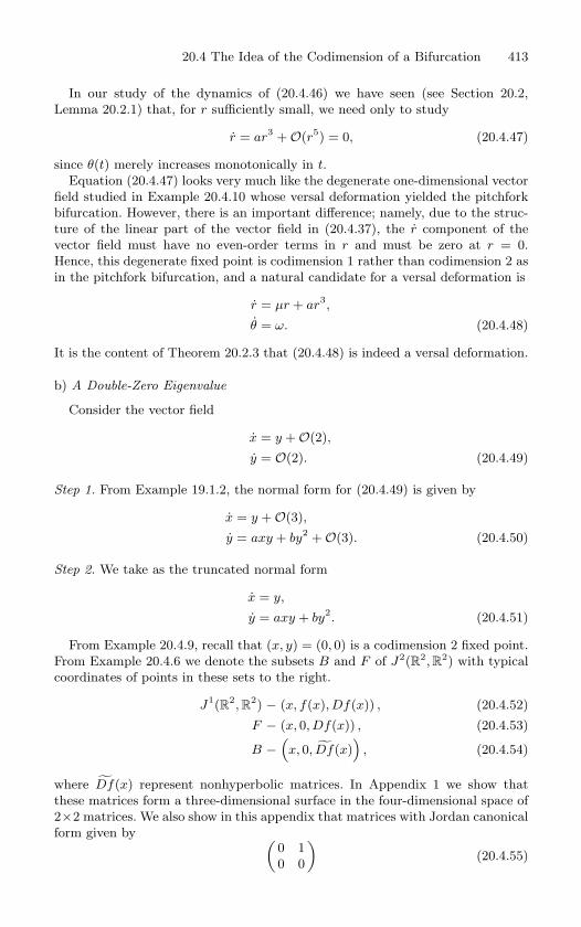
20.4 The Idea of the Codimension of a Bifurcation 413
In our study of the dynamics of (20.4.46) we have seen (see Section 20.2,
Lemma 20.2.1) that, for r sufficiently small, we need only to study
r = ar3+ O(r5
) = 0, (20.4.47)
since θ(t) merely increases monotonically in t.Equation (20.4.47) looks very much like the degenerate one-dimensional vector
field studied in Example 20.4.10 whose versal deformation yielded the pitchfork
bifurcation. However, there is an important difference; namely, due to the struc-
ture of the linear part of the vector field in (20.4.37), the r component of the
vector field must have no even-order terms in r and must be zero at r = 0.
Hence, this degenerate fixed point is codimension 1 rather than codimension 2 as
in the pitchfork bifurcation, and a natural candidate for a versal deformation is
r = µr + ar3,
θ = ω. (20.4.48)
It is the content of Theorem 20.2.3 that (20.4.48) is indeed a versal deformation.
b) A Double-Zero Eigenvalue
Consider the vector field
x = y + O(2),
y = O(2). (20.4.49)
Step 1. From Example 19.1.2, the normal form for (20.4.49) is given by
x = y + O(3),
y = axy + by2+ O(3). (20.4.50)
Step 2. We take as the truncated normal form
x = y,
y = axy + by2. (20.4.51)
From Example 20.4.9, recall that (x, y) = (0, 0) is a codimension 2 fixed point.
From Example 20.4.6 we denote the subsets B and F of J2(R2, R2) with typical
coordinates of points in these sets to the right.
J1(R
2, R2) − (x, f(x), Df(x)) , (20.4.52)
F − (x, 0, Df(x)) , (20.4.53)
B −(x, 0, Df(x)
), (20.4.54)
where Df(x) represent nonhyperbolic matrices. In Appendix 1 we show that
these matrices form a three-dimensional surface in the four-dimensional space of
2×2 matrices. We also show in this appendix that matrices with Jordan canonical
form given by (0 1
0 0
)(20.4.55)
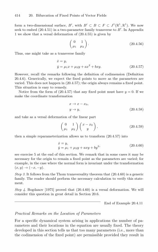
414 20. Bifurcation of Fixed Points of Vector Fields
form a two-dimensional surface, B′, with B′ ⊂ B ⊂ F ⊂ J1(R1, R1). We now
seek to embed (20.4.51) in a two-parameter family transverse to B′. In Appendix
1 we show that a versal deformation of (20.4.55) is given by(0 1
µ1 µ2
). (20.4.56)
Thus, one might take as a transverse family
x = y,
y = µ1x + µ2y + ax2+ bxy. (20.4.57)
However, recall the remarks following the definition of codimension (Definition
20.4.6). Generically, we expect the fixed points to move as the parameters are
varied. This does not happen in (20.4.57); the origin always remains a fixed point.
This situation is easy to remedy.
Notice from the form of (20.4.57) that any fixed point must have y = 0. If we
make the coordinate transformation
x → x − x0,
y → y, (20.4.58)
and take as a versal deformation of the linear part(0 1
µ1 µ2
)(x − x0
y
), (20.4.59)
then a simple reparameterization allows us to transform (20.4.57) into
x = y,y = µ1 + µ2y + axy + by2, (20.4.60)
see exercise 5 at the end of this section. We remark that in some cases it may be
necessary for the origin to remain a fixed point as the parameters are varied; for
example, in the case where the normal form is invariant under the transformation
(x, y) → (−x, −y).
Step 3. It follows from the Thom transversality theorem that (20.4.60) is a generic
family. The reader should perform the necessary calculation to verify this state-
ment.
Step 4. Bogdanov [1975] proved that (20.4.60) is a versal deformation. We will
consider this question in great detail in Section 20.6.
End of Example 20.4.11
Practical Remarks on the Location of Parameters
For a specific dynamical system arising in applications the number of pa-rameters and their locations in the equation are usually fixed. The theorydeveloped in this section tells us that too many parameters (i.e., more thanthe codimension of the fixed point) are permissible provided they result in
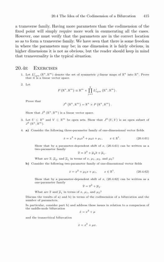
20.4 The Idea of the Codimension of a Bifurcation 415
a transverse family. Having more parameters than the codimension of thefixed point will simply require more work in enumerating all the cases.However, one must verify that the parameters are in the correct locationso as to form a transverse family. We have seen that there is some freedomin where the parameters may be; in one dimension it is fairly obvious, inhigher dimensions it is not as obvious, but the reader should keep in mindthat transversality is the typical situation.
20.4e Exercises1. Let Lj
sym (Rn, Rm) denote the set of symmetric j-linear maps of R
n into Rn. Prove
that it is a linear vector space.
2. Let
P(R
n, R
m)≡ R
m ×k∏
j=1
Ljsym
(R
n, R
m).
Prove thatJ
k (R
n, R
m)= R
n × P(R
n, R
m).
Show that Jk (Rn, Rm) is a linear vector space.
3. Let U ⊂ Rn and V ⊂ R
m be open sets. Show that Jk (U, V ) is an open subset ofJk (Rn, R
m).
4. a) Consider the following three-parameter family of one-dimensional vector fields
x = x3 + µ3x
2 + µ2x + µ1, x ∈ R1. (20.4.61)
Show that by a parameter-dependent shift of x, (20.4.61) can be written as atwo-parameter family
x = x3 + µ2x + µ1.
What are x, µ2, and µ1 in terms of x, µ1, µ2, and µ3?
b) Consider the following two-parameter family of one-dimensional vector fields
x = x2 + µ2x + µ1, x ∈ R
1. (20.4.62)
Show that by a parameter-dependent shift of x, (20.4.62) can be written as aone-parameter family
x = x2 + µ1.
What are x and µ1 in terms of x, µ1, and µ2?
Discuss the results of a) and b) in terms of the codimension of a bifurcation and thenumber of parameters.
In particular, consider part b) and address these issues in relation to a comparison ofthe saddle-node bifurcation
x = x2 + µ
and the transcritical bifurcation
x = x2 + µx.
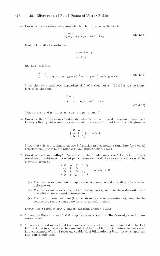
416 20. Bifurcation of Fixed Points of Vector Fields
5. Consider the following two-parameter family of planar vector fields
x = y,
y = µ1x + µ2y + ax2 + bxy.
(20.4.63)
Under the shift of coordinates
x → x + x0,
y → y,
(20.4.63) becomes
x = y,
y = µ1x0 + µ1x + µ2y + a(x2 + 2xx0 + x20) + b(x0 + x)y.
(20.4.64)
Show that by a parameter-dependent shift of y (but not x), (20.4.63) can be trans-formed to the form
x = y,
y = µ1 + µ2y + ax2 + bxy.
(20.4.65)
What are µ1 and µ2 in terms of x0, µ1, µ2, a, and b?
6. Consider the “Hopf-steady state interaction”, i.e., a three dimensional vector fieldhaving a fixed point where the (real) Jordan canonical form of the matrix is given by
0 −ω 0
ω 0 00 0 0
, ω > 0.
Show that this is a codimension two bifurcation and compute a candidate for a versaldeformation. (Hint: Use Example 20.5.6 from Section 20.5.)
7. Consider the “double-Hopf bifurcation” or the “mode interaction”, i.e., a four dimen-sional vector field having a fixed point where the (real) Jordan canonical form of thematrix is given by
0 −ω1 0 0
ω1 0 0 00 0 0 −ω20 0 ω2 0
, ω1, ω2 > 0.
(a) For the nonresonant case, compute the codimension and a candidate for a versaldeformation.
(b) For the resonant case (except for 1 : 1 resonance), compute the codimension anda candidate for a versal deformation.
(c) For the 1 : 1 resonant case (both semisimple and non-semisimple), compute thecodimension and a candidate for a versal deformation.
(Hint: Use Examples 20.5.7 and 20.5.8 from Section 20.5.)
8. Survey the literature and find five applications where the “Hopf- steady state” bifur-cation arises.
9. Survey the literature and find five applications where the a) non- resonant double-Hopfbifurcation arises, b) where the resonant double- Hopf bifurcation arises. In particular,find an example of a 1 : 1 resonant double-Hopf bifurcation in both the semsimple andnon- semisimple case.
20.5 Versal Deformations of Families of Matrices 417
20.5 Versal Deformations of Families of Matrices
In this section we develop the theory of versal deformations of matriceswhich we use in computing versal deformations of fixed points of dynamicalsystems. Our discussion follows Arnold [1983]. Let M be the space of n×n matrices with complex entries. The relation of similarity of matricespartitions the entire space into manifolds consisting of matrices havingthe same eigenvalues and dimensions of Jordan blocks; this partitioning iscontinuous, since the eigenvalues vary continuously.
Suppose we have a matrix having some identical eigenvalues, and we wantto reduce it to Jordan canonical form. This process is not stable, becausethe slightest perturbation might destroy the Jordan canonical form com-pletely. Thus, if the matrix is only approximately known (or the reductionis attempted by computer), then the procedure may yield nonsense.
We give an example. Consider the matrix
A(λ) =(
0 λ0 0
).
The Jordan canonical form is given by(0 10 0
), λ = 0,
with conjugating matrix
C(λ) =(
1 00 1/λ
), λ = 0.
Now, at λ = 0, the Jordan canonical form of A(λ) is given by(0 00 0
),
with conjugating matrix
C(0) =(
1 00 1
).
Therefore, C(λ) is discontinuous at λ = 0.However, even though multiple eigenvalues is an unstable situation for
individual matrices, it is stable for parametrized families of matrices, i.e.,perturbing the family does not remove the multiple eigenvalue matrix fromthe family. Thus, while we can reduce every member of the family to Jordancanonical form (as in the example above), in general, the transformationwill depend discontinuously on the parameter. The problem we address isthe following:
418 20. Bifurcation of Fixed Points of Vector Fields
What is the simplest form to which a family of matrices can be
reduced depending differentiably on the parameters by a change
of parameters depending differentiably on the parameters?
In the following we will construct such families and determine the mini-mum number of parameters, but first we must begin with some definitionsand develop some necessary machinery.
We will consider n×n matrices whose entries are complex numbers. LetA0 be such a matrix. The reason that we will be dealing (initially) withcomplex matrices is that the Jordan canonical form is more simple in thissetting. Afterwards, we will show how the results obtained in the complexsetting can be used for matrices with real entries.
We first need to introduce several definitions.
Definition 20.5.1 (Deformation of a Matrix) A deformation of A0 is
a Cr (r ≥ 1) mapping
A : Λ→ Cn2
,
λ→ A(λ),
where Λ ∈ C is some parameter space and
A(λ0) = A0.
A deformation is also called a family, the variables λi, i = 1, · · · , , are
called the parameters, and Λ is called the base of the family.
Definition 20.5.2 (Equivalence of Deformations) Two deformations
A(λ), B(λ) of A0 are called equivalent if there exists a deformation of the
identity matrix C(λ) (C(λ0) = id) with the same base such that
B(λ) = C(λ)A(λ)C−1(λ).
The following idea will be useful for reparametrizing families of matricesin order to reduce the number of parameters.
Definition 20.5.3 (Family Induced from a Deformation) Let Σ ⊂C
m, Λ ⊂ C be open sets. Consider the Cr (r ≥ 1) mapping
φ : Σ→ Λ,
µ→ φ(µ),
with φ(µ0) = λ0.
The family induced from A by the mapping φ is called (φ∗A)(µ) and is
defined by
(φ∗A)(µ) ≡ A(φ(µ)), µ ∈ Cm.
20.5 Versal Deformations of Families of Matrices 419
Definition 20.5.4 (Versal, Miniversal, and Universal Deforma-tions) A deformation A(λ) of a matrix A0 is said to be versal if any
deformation B(µ) of A0 is equivalent to a deformation induced from A,
i.e.,
B(µ) = C(µ)A(φ(µ))C−1(µ)
for some change of parameters
φ : Σ → Λ,
with C(µ0) = id and φ(µ0) = λ0.
A versal deformation is said to be universal if the inducing mapping (i.e.,
change of parameters map) is determined uniquely by the deformation B.
A versal deformation is said to be miniversal if the dimension of the
parameter space is the smallest possible for a versal deformation.
At this stage it is useful to consider an example.
Example 20.5.1. Consider the matrix
A0 =
(0 1
0 0
).
It should be clear that a versal deformation of A0 is given by
B(µ) ≡(
0 1
0 0
)+
(µ1 µ2
µ3 µ4
),
where µ ≡ (µ1, µ2, µ3, µ4) ∈ C4. However, B(µ) is not miniversal; a miniversal
deformation is given by
A(λ) =
(0 1
0 0
)+
(0 0
λ1 λ2
),
where λ = (λ1, λ2) ∈ C2. This can be seen by showing that B(µ) is equivalent to
a deformation induced from A(λ). If we let
C(µ) =
(1 + µ2 0
−µ1 1
), C−1
(µ) =1
1 + µ2
(1 0
µ1 1 + µ2
),
then it follows that
A(λ) = A(φ(µ)) = C−1(µ)B(µ)C(µ)
=
(0 1
0 0
)+
(0 0
µ3(1 + µ2) − µ1µ4 µ1 + µ4
),
where we take
φ(µ) = (φ1(µ), φ2(µ)) = (µ3(1 + µ2) − µ1µ4, µ1 + µ4) ≡ (λ1, λ2) ≡ λ
as the inducing mapping.
End of Example 20.5.1
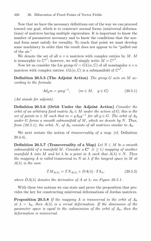
420 20. Bifurcation of Fixed Points of Vector Fields
Now that we have the necessary definitions out of the way we can proceedtoward our goal, which is to construct normal forms (miniversal deforma-tions) of matrices having multiple eigenvalues. It is important to know thenumber of parameters necessary and to know the conditions that the nor-mal form must satisfy for versality. To reach that point we must developsome machinery in order that the result does not appear to be “pulled outof the air.”
We denote the set of all n × n matrices with complex entries by M . Mis isomorphic to C
n2; however, we will simply write M = C
n2.
Now let us consider the Lie group G = GL(n, C) of all nonsingular n×n
matrices with complex entries. GL(n, C) is a submanifold of Cn2
.
Definition 20.5.5 (The Adjoint Action) The group G acts on M ac-
cording to the formula
Adgm = gmg−1, (m ∈ M, g ∈ G) (20.5.1)
(Ad stands for adjoint).
Definition 20.5.6 (Orbit Under the Adjoint Action) Consider the
orbit of an arbitrary fixed matrix A0 ∈ M under the action of G; this is the
set of points m ∈ M such that m = gA0g−1 for all g ∈ G. The orbit of A0
under G forms a smooth submanifold of M , which we denote by N . Thus,
from (20.5.1), the orbit, N , of A0 consists of all matrices similar to A0.
We next restate the notion of transversality of a map. (cf. Definition20.4.4).
Definition 20.5.7 (Transversality of a Map) Let N ⊂ M be a smooth
submanifold of a manifold M . Consider a Cr (r ≥ 1) mapping of another
manifold Λ into M and let λ be a point in Λ such that A(λ) ∈ N . Then
the mapping A is called transversal to N at λ if the tangent space to M at
A(λ) is the sum
TMA(λ) = TNA(λ) + DA(λ) · TΛλ, (20.5.2)
where DA(λ) denotes the derivative of A at λ; see Figure 20.5.1.
With these two notions we can state and prove the proposition that pro-vides the key for constructing miniversal deformations of Jordan matrices.
Proposition 20.5.8 If the mapping A is transversal to the orbit of A0at λ = λ0, then A(λ) is a versal deformation. If the dimension of the
parameter space is equal to the codimension of the orbit of A0, then the
deformation is miniversal.
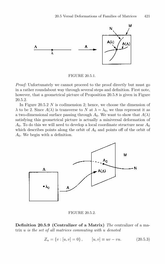
20.5 Versal Deformations of Families of Matrices 421
FIGURE 20.5.1.
Proof: Unfortunately we cannot proceed to the proof directly but must goin a rather roundabout way through several steps and definition. First note,however, that a geometrical picture of Proposition 20.5.8 is given in Figure20.5.2.
In Figure 20.5.2 N is codimension 2; hence, we choose the dimension ofλ to be 2. Since A(λ) is transverse to N at λ = λ0, we thus represent it asa two-dimensional surface passing through A0. We want to show that A(λ)satisfying this geometrical picture is actually a miniversal deformation ofA0. To do this we will need to develop a local coordinate structure near A0which describes points along the orbit of A0 and points off of the orbit ofA0. We begin with a definition.
FIGURE 20.5.2.
Definition 20.5.9 (Centralizer of a Matrix) The centralizer of a ma-trix u is the set of all matrices commuting with u denoted
Zu = v : [u, v] = 0 , [u, v] ≡ uv − vu. (20.5.3)
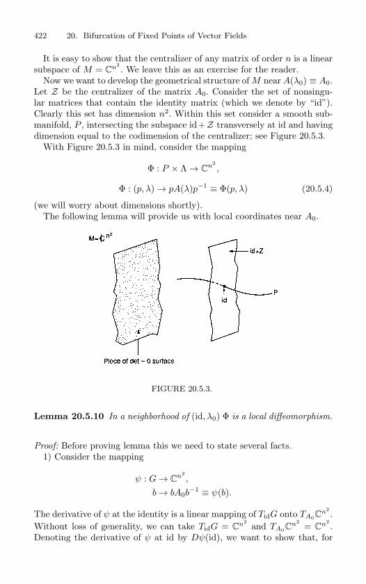
422 20. Bifurcation of Fixed Points of Vector Fields
It is easy to show that the centralizer of any matrix of order n is a linearsubspace of M = C
n2. We leave this as an exercise for the reader.
Now we want to develop the geometrical structure of M near A(λ0) ≡ A0.Let Z be the centralizer of the matrix A0. Consider the set of nonsingu-lar matrices that contain the identity matrix (which we denote by “id”).Clearly this set has dimension n2. Within this set consider a smooth sub-manifold, P , intersecting the subspace id+Z transversely at id and havingdimension equal to the codimension of the centralizer; see Figure 20.5.3.
With Figure 20.5.3 in mind, consider the mapping
Φ : P × Λ → Cn2
,
Φ : (p, λ) → pA(λ)p−1 ≡ Φ(p, λ) (20.5.4)
(we will worry about dimensions shortly).The following lemma will provide us with local coordinates near A0.
FIGURE 20.5.3.
Lemma 20.5.10 In a neighborhood of (id, λ0) Φ is a local diffeomorphism.
Proof: Before proving lemma this we need to state several facts.1) Consider the mapping
ψ : G→ Cn2
,
b→ bA0b−1 ≡ ψ(b).
The derivative of ψ at the identity is a linear mapping of TidG onto TA0Cn2
.Without loss of generality, we can take TidG = C
n2and TA0C
n2= C
n2.
Denoting the derivative of ψ at id by Dψ(id), we want to show that, for
20.5 Versal Deformations of Families of Matrices 423
u ∈ Cn2
, Dψ(id)u is given by the operation of commutation of u with A0,i.e., Dψ(id)u = [u,A0].
This is easily calculated as follows
Dψ(id)u = limε→0
(id + εu)A0(id + εu)−1 −A0
ε
= limε→0
(A0 + εuA0)(id− εu) +O(ε2)−A0
ε
= limε→0
A0 − εA0u + εuA0 +O(ε2)−A0
ε= uA0 −A0u ≡ [u, A0];
therefore,Dψ(id) : C
n2 → Cn2
,u → [u, A0].
(20.5.5)
We make the following observation. Since dimG = dimM = n2, the di-mension of the centralizer is equal to the codimension of the orbit of A0.This is because, roughly speaking, from (20.5.1) and (20.5.4) we can thinkof the centralizer of A0 to be the matrices that do not change A0. Thus,we have
dimZ = dimΛ, (20.5.6)
dimP = dimN, (20.5.7)
anddim Λ + dimN = n2.
Now, returning to Φ,Φ : P × Λ → C
n2.
From (20.5.6) and (20.5.7) we see that the dimensions are consistent (i.e.,dim(P × Λ) = dim C
n2) for Φ to be a diffeomorphism.
We can now finally prove Lemma 20.5.10. We compute the derivative ofΦ at (id, λ0), denoted DΦ(id, λ0), and examine how it acts on a typicalelement of T(id,λ0)(P × Λ). Let (u, λ) ∈ T(id,λ0)(P × Λ); then we have
DΦ(id, λ0)(u, λ) = (DpΦ(id, λ0), DλΦ(id, λ0))(u, λ). (20.5.8)
Using (20.5.4) and (20.5.5) it is easy to see that (20.5.8) is given by
DΦ(id, λ0)(u, λ) = ([u, A0], DA(λ0)λ). (20.5.9)
By construction of the submanifold P , DpΦ(id, λ0) maps TidP isomorphi-cally to a space tangent to the orbit N at A0 (check dimensions and thefact that [u,A0] = 0). Also by the hypothesis of Proposition 20.5.8, DA(λ0)maps Tλ0Λ isomorphically to a space transverse to N at A(λ0) = A0. Con-sequently, DΦ(id, λ0) is an isomorphism between linear spaces of dimension
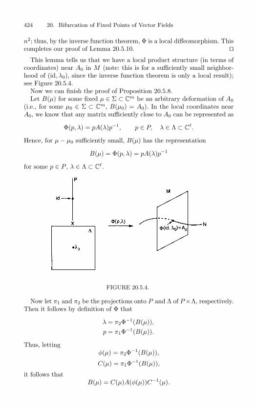
424 20. Bifurcation of Fixed Points of Vector Fields
n2; thus, by the inverse function theorem, Φ is a local diffeomorphism. Thiscompletes our proof of Lemma 20.5.10.
This lemma tells us that we have a local product structure (in terms ofcoordinates) near A0 in M (note: this is for a sufficiently small neighbor-hood of (id, λ0), since the inverse function theorem is only a local result);see Figure 20.5.4.
Now we can finish the proof of Proposition 20.5.8.Let B(µ) for some fixed µ ∈ Σ ⊂ C
m be an arbitrary deformation of A0(i.e., for some µ0 ∈ Σ ⊂ C
m, B(µ0) = A0). In the local coordinates nearA0, we know that any matrix sufficiently close to A0 can be represented as
Φ(p, λ) = pA(λ)p−1, p ∈ P, λ ∈ Λ ⊂ C.
Hence, for µ− µ0 sufficiently small, B(µ) has the representation
B(µ) = Φ(p, λ) = pA(λ)p−1
for some p ∈ P , λ ∈ Λ ⊂ C.
FIGURE 20.5.4.
Now let π1 and π2 be the projections onto P and Λ of P×Λ, respectively.Then it follows by definition of Φ that
λ = π2Φ−1(B(µ)),p = π1Φ−1(B(µ)).
Thus, lettingφ(µ) = π2Φ−1(B(µ)),
C(µ) = π1Φ−1(B(µ)),
it follows thatB(µ) = C(µ)A(φ(µ))C−1(µ).
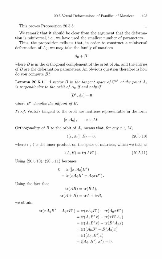
20.5 Versal Deformations of Families of Matrices 425
This proves Proposition 20.5.8. We remark that it should be clear from the argument that the deforma-
tion is miniversal, i.e., we have used the smallest number of parameters.Thus, the proposition tells us that, in order to construct a miniversal
deformation of A0, we may take the family of matrices
A0 + B,
where B is in the orthogonal complement of the orbit of A0, and the entriesof B are the deformation parameters. An obvious question therefore is howdo you compute B?
Lemma 20.5.11 A vector B in the tangent space of Cn2
at the point A0is perpendicular to the orbit of A0 if and only if
[B∗, A0] = 0
where B∗ denotes the adjoint of B.
Proof: Vectors tangent to the orbit are matrices representable in the form
[x,A0] , x ∈ M.
Orthogonality of B to the orbit of A0 means that, for any x ∈ M ,
〈[x,A0] , B〉 = 0, (20.5.10)
where 〈 , 〉 is the inner product on the space of matrices, which we take as
〈A, B〉 = tr(AB∗). (20.5.11)
Using (20.5.10), (20.5.11) becomes
0 = tr ([x,A0]B∗)= tr (xA0B
∗ −A0xB∗) .
Using the fact thattr(AB) = tr(BA),
tr(A + B) = trA + trB,
we obtain
tr(xA0B∗ −A0xB∗) = tr(xA0B
∗)− tr(A0xB∗)= tr(A0B
∗x)− tr(xB∗A0)= tr(A0B
∗x)− tr(B∗A0x)= tr((A0B
∗ −B∗A0)x)= tr([A0, B
∗]x)= 〈[A0, B
∗], x∗〉 = 0.
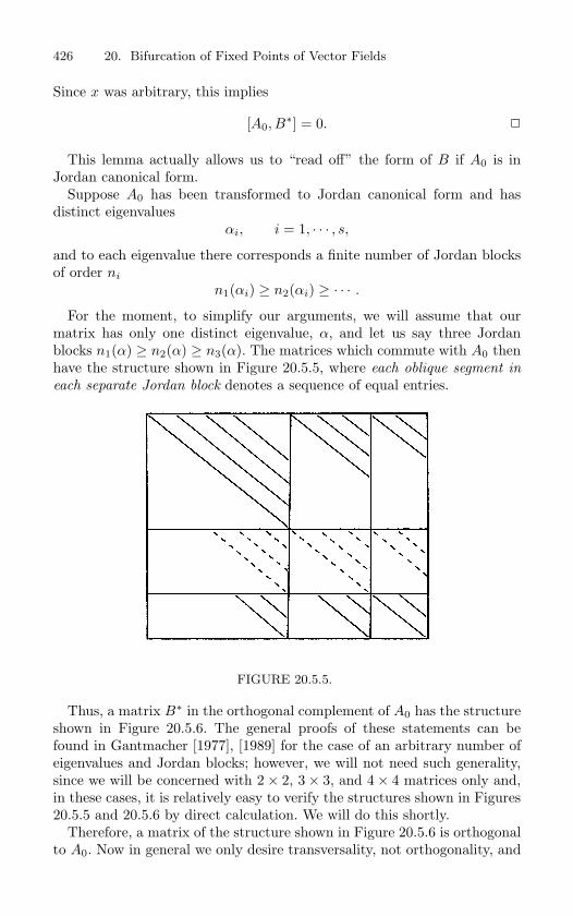
426 20. Bifurcation of Fixed Points of Vector Fields
Since x was arbitrary, this implies
[A0, B∗] = 0.
This lemma actually allows us to “read off” the form of B if A0 is inJordan canonical form.
Suppose A0 has been transformed to Jordan canonical form and hasdistinct eigenvalues
αi, i = 1, · · · , s,and to each eigenvalue there corresponds a finite number of Jordan blocksof order ni
n1(αi) ≥ n2(αi) ≥ · · · .
For the moment, to simplify our arguments, we will assume that ourmatrix has only one distinct eigenvalue, α, and let us say three Jordanblocks n1(α) ≥ n2(α) ≥ n3(α). The matrices which commute with A0 thenhave the structure shown in Figure 20.5.5, where each oblique segment in
each separate Jordan block denotes a sequence of equal entries.
FIGURE 20.5.5.
Thus, a matrix B∗ in the orthogonal complement of A0 has the structureshown in Figure 20.5.6. The general proofs of these statements can befound in Gantmacher [1977], [1989] for the case of an arbitrary number ofeigenvalues and Jordan blocks; however, we will not need such generality,since we will be concerned with 2× 2, 3× 3, and 4× 4 matrices only and,in these cases, it is relatively easy to verify the structures shown in Figures20.5.5 and 20.5.6 by direct calculation. We will do this shortly.
Therefore, a matrix of the structure shown in Figure 20.5.6 is orthogonalto A0. Now in general we only desire transversality, not orthogonality, and
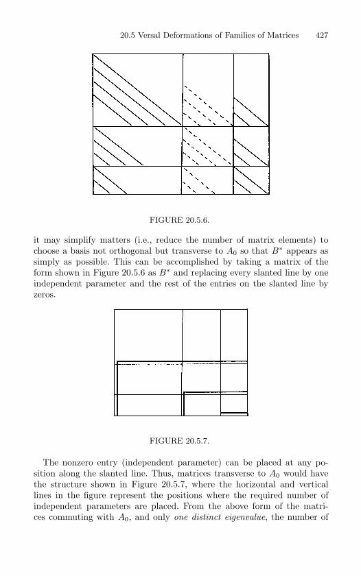
20.5 Versal Deformations of Families of Matrices 427
FIGURE 20.5.6.
it may simplify matters (i.e., reduce the number of matrix elements) tochoose a basis not orthogonal but transverse to A0 so that B∗ appears assimply as possible. This can be accomplished by taking a matrix of theform shown in Figure 20.5.6 as B∗ and replacing every slanted line by oneindependent parameter and the rest of the entries on the slanted line byzeros.
FIGURE 20.5.7.
The nonzero entry (independent parameter) can be placed at any po-sition along the slanted line. Thus, matrices transverse to A0 would havethe structure shown in Figure 20.5.7, where the horizontal and verticallines in the figure represent the positions where the required number ofindependent parameters are placed. From the above form of the matri-ces commuting with A0, and only one distinct eigenvalue, the number of
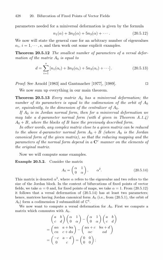
428 20. Bifurcation of Fixed Points of Vector Fields
parameters needed for a miniversal deformation is given by the formula
n1(α) + 3n2(α) + 5n3(α) + · · · . (20.5.12)
We now will state the general case for an arbitrary number of eigenvaluesαi, i = 1, · · · , s, and then work out some explicit examples.
Theorem 20.5.12 The smallest number of parameters of a versal defor-
mation of the matrix A0 is equal to
d =s∑
i=1
[n1(αi) + 3n2(αi) + 5n3(αi) + · · ·] . (20.5.13)
Proof: See Arnold [1983] and Gantmacher [1977], [1989]. We now sum up everything in our main theorem.
Theorem 20.5.13 Every matrix A0 has a miniversal deformation; the
number of its parameters is equal to the codimension of the orbit of A0or, equivalently, to the dimension of the centralizer of A0.
If A0 is in Jordan normal form, then for a miniversal deformation we
may take a d-parameter normal form (with d given in Theorem A.1.4)
A0 + B, where the blocks of B have the previously described form.
In other words, any complex matrix close to a given matrix can be reduced
to the above d-parameter normal form A0 + B (where A0 is the Jordan
canonical form of the given matrix), so that the reducing mapping and the
parameters of the normal form depend in a Cr manner on the elements of
the original matrix.
Now we will compute some examples.
Example 20.5.2. Consider the matrix
A0 =
(α 1
0 α
), α2. (20.5.14)
This matrix is denoted α2, where α refers to the eigenvalue and two refers to the
size of the Jordan block. In the context of bifurcations of fixed points of vector
fields, we take α = 0 and, for fixed points of maps, we take α = 1. From (20.5.12)
it follows that a versal deformation of (20.5.14) has at least two parameters;
hence, matrices having Jordan canonical form A0 (i.e., from (20.5.1), the orbit of
A0) form a codimension 2 submanifold of C4.
We now want to compute a versal deformation for A0. First we compute a
matrix which commutes with A0.(a bc d
)(α 1
0 α
)−
(α 1
0 α
)(a bc d
)=
(aα a + bαcα c + dα
)−
(aα + c bα + d
αc αd
)=
(−c a − d0 c
)=
(0 0
0 0
);
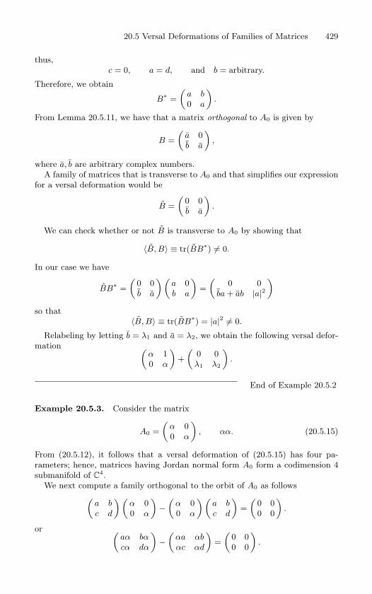
20.5 Versal Deformations of Families of Matrices 429
thus,
c = 0, a = d, and b = arbitrary.
Therefore, we obtain
B∗=
(a b0 a
).
From Lemma 20.5.11, we have that a matrix orthogonal to A0 is given by
B =
(a 0
b a
),
where a, b are arbitrary complex numbers.
A family of matrices that is transverse to A0 and that simplifies our expression
for a versal deformation would be
B =
(0 0
b a
).
We can check whether or not B is transverse to A0 by showing that
〈B, B〉 ≡ tr(BB∗) = 0.
In our case we have
BB∗=
(0 0
b a
)(a 0
b a
)=
(0 0
ba + ab |a|2)
so that
〈B, B〉 ≡ tr(BB∗) = |a|2 = 0.
Relabeling by letting b = λ1 and a = λ2, we obtain the following versal defor-
mation (α 1
0 α
)+
(0 0
λ1 λ2
).
End of Example 20.5.2
Example 20.5.3. Consider the matrix
A0 =
(α 0
0 α
), αα. (20.5.15)
From (20.5.12), it follows that a versal deformation of (20.5.15) has four pa-
rameters; hence, matrices having Jordan normal form A0 form a codimension 4
submanifold of C4.
We next compute a family orthogonal to the orbit of A0 as follows(a bc d
)(α 0
0 α
)−
(α 0
0 α
)(a bc d
)=
(0 0
0 0
).
or (aα bαcα dα
)−
(αa αbαc αd
)=
(0 0
0 0
).
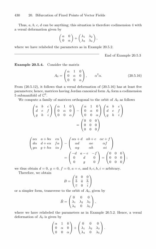
430 20. Bifurcation of Fixed Points of Vector Fields
Thus, a, b, c, d can be anything; this situation is therefore codimension 4 with
a versal deformation given by(α 0
0 α
)+
(λ1 λ2
λ3 λ4
),
where we have relabeled the parameters as in Example 20.5.2.
End of Example 20.5.3
Example 20.5.4. Consider the matrix
A0 =
α 1 0
0 α 0
0 0 α
, α2α. (20.5.16)
From (20.5.12), it follows that a versal deformation of (20.5.16) has at least five
parameters; hence, matrices having Jordan canonical form A0 form a codimension
5 submanifold of C9.
We compute a family of matrices orthogonal to the orbit of A0 as follows a b cd e fg h i
α 1 0
0 α 0
0 0 α
−α 1 0
0 α 0
0 0 α
a b cd e fg h i
=
0 0 0
0 0 0
0 0 0
aα a + bα cα
dα d + eα fαgα g + hα iα
− aα + d αb + e αc + f
αd αe αfαg αh αi
=
−d a − e −f0 d 0
0 g 0
=
0 0 0
0 0 0
0 0 0
;
we thus obtain d = 0, g = 0, f = 0, a = e, and b, c, h, i = arbitrary.
Therefore, we obtain
B =
a 0 0
b a hc 0 i
or a simpler form, transverse to the orbit of A0, given by
B =
0 0 0
λ1 λ2 λ3
λ4 0 λ5
,
where we have relabeled the parameters as in Example 20.5.2. Hence, a versal
deformation of A0 is given byα 1 0
0 α 0
0 0 α
+
0 0 0
λ1 λ2 λ3
λ4 0 λ5
.
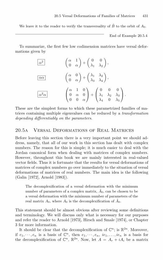
20.5 Versal Deformations of Families of Matrices 431
We leave it to the reader to verify the transversality of B to the orbit of A0.
End of Example 20.5.4
To summarize, the first few low codimension matrices have versal defor-mations given by
α2(
α 10 α
)+
(0 0λ1 λ2
),
αα
(α 00 α
)+
(λ1 λ2λ3 λ4
),
α2α
α 1 0
0 α 00 0 α
+
0 0 0
λ1 λ2 λ3λ4 0 λ5
.
These are the simplest forms to which these parametrized families of ma-trices containing multiple eigenvalues can be reduced by a transformation
depending differentiably on the parameters.
20.5a Versal Deformations of Real MatricesBefore leaving this section there is a very important point we should ad-dress, namely, that all of our work in this section has dealt with complexnumbers. The reason for this is simple; it is much easier to deal with theJordan canonical form when dealing with matrices of complex numbers.However, throughout this book we are mainly interested in real-valuedvector fields. Thus it is fortunate that the results for versal deformations ofmatrices of complex numbers go over immediately to the situation of versaldeformations of matrices of real numbers. The main idea is the following(Galin [1972], Arnold [1983]).
The decomplexification of a versal deformation with the minimum
number of parameters of a complex matrix, A0, can be chosen to be
a versal deformation with the minimum number of parameters of the
real matrix A0, where A0 is the decomplexification of A0.
This statement should be almost obvious after reviewing some definitionsand terminology. We will discuss only what is necessary for our purposesand refer the reader to Arnold [1973], Hirsch and Smale [1974], or Chapter3 for more information.
It should be clear that the decomplexification of Cn; is R
2n. Moreover,if e1, · · · , en is a basis of C
n, then e1, · · · , en, ie1, . . . , ien is a basis forthe decomplexification of C
n, R2n. Now, let A = Ar + iAi be a matrix
432 20. Bifurcation of Fixed Points of Vector Fields
representation of some complex linear operator mapping Cn into itself.
Then the decomplexification of this matrix is given by the 2n× 2n matrix(Ar −Ai
Ai Ar
). (20.5.17)
Now we show how we can use these ideas to construct a versal deforma-tion of a real matrix. As in the complex case, the construction of a versaldeformation of a matrix in Jordan canonical form is carried out “Jordanblock by Jordan block”. Therfore we really only need to understand thecase of a real matrix having exactly two complex eigenvalues (complexconjugate pairs).
Consider a real matrix
A0 : R2n → R
2n,
and suppose that it has exactly two eigenvalues
α± iβ, β = 0,
and each eigenvalue has corresponding Jordan blocks of dimension
n1 ≥ n2 ≥ n3 ≥ · · · , with n1 + n2 + n3 + · · · = n.
Using the theory of the real Jordan canonical form, we can construct areal basis in R
2n with respect to which A0 has the form of the matrix ofthe decomplexification of the Jordan canonical form of the complex matrix
A0 : Cn → C
n,
where A0 has only one eigenvalue, α+iβ, with Jordan blocks of dimensionsn1 ≥ n2 ≥ n3 ≥ · · · , with n1 + n2 + n3 + · · · = n, i.e.,
A0 =(
J −βidβid J
),
where id denotes the n × n identity matrix and J is the upper triangularreal Jordan matrix with eigenvalue α and blocks of dimension n1 ≥ n2 ≥n3 ≥ · · · , with n1 + n2 + n3 + · · · = n. Then a versal deformation for A0 isconstructed from a versal deformation of A0 as follows.
With A0 in Jordan canonical form, construct the versal deformation
according the the methods for complex matrices developed above.
Then decomplexify the result according to (20.5.17).
As we have noted, the construction of a versal deformation of a matrixin Jordan canonical form is carried out “Jordan block by Jordan block”.Therefore if the eigenvalues of a matrix are all real, we see that there is
20.5 Versal Deformations of Families of Matrices 433
no difference with the theory developed for the case of complex matrices.If there are complex eigenvalues, versal deformations for the correspondingJordan blocks are constructed as described above.
Moreover, we also see immediately that the minimum number of param-eters of a real versal deformation are also given by the formula:
d =∑
λ
(n1(λ) + 3n2(λ) + 5n3(λ) · · ·) ,
where the summation is over all s eigenvalues, both real and complex.We next consider some examples.
Example 20.5.5 (An Imaginary Pair of Eigenvalues).
Consider a 2 × 2 real matrix having eigenvalues ρ + iτ . Then with respect to
an appropriate basis it has the form
A0 =
(ρ −ττ ρ
).
We want to construct a versal deformation of this matrix.
The complexification of A0 is given by
A0 = (α) , α ≡ ρ + iτ.
According to Theorem 20.5.12, a versal deformation for A0 can be constructed
with one (complex) parameter, λ = µ + iγ, i.e, the versal deformation of A0 is
given by
(α) + (λ) .
With this result, and (20.5.17), a versal deformation of A0 is given by(ρ −ττ ρ
)+
(µ −γγ µ
).
End of Example 20.5.5
Examples 20.5.6, and 20.5.7 use the fact that versal deformations areconstructed Jordan block-by-block, versal deformations of Jordan blockscorresponding to real eigenvalues are exactly the same as in the complexcase (with real parameters), and example 20.5.5.
Example 20.5.6 (One Real, and A Pure Imaginary Pair of Eigenvalues).
Consider a 3 × 3 real matrix having eigenvalues ρ ± iτ, β, τ = 0. Then with
respect to an appropriate basis it has the form
A0 =
ρ −τ 0
τ ρ 0
0 0 β
.
434 20. Bifurcation of Fixed Points of Vector Fields
A versal deformation requires three real parameters and is given by ρ −τ 0
τ ρ 0
0 0 β
+
µ −γ 0
γ µ 0
0 0 δ
.
End of Example 20.5.6
Example 20.5.7 (A Pair of Distinct, Imaginary Pairs of Eigenvalues).
Consider a 4 × 4 real matrix having eigenvalues αi = ρi + iτi, i = 1, 2, with
α1 = α2. Then with respect to an appropriate basis it has the form
A0 =
ρ1 −τ1 0 0
τ1 ρ1 0 0
0 0 ρ2 −τ2
0 0 τ2 ρ2
.
This matrix is simple two Jordan blocks of example 20.5.5. Hence, using the result
from example 20.5.5, a versal deformation of A0 requires four real parameters and
is given by ρ1 −τ1 0 0
τ1 ρ1 0 0
0 0 ρ2 −τ2
0 0 τ2 ρ2
+
µ1 −γ1 0 0
γ1 µ1 0 0
0 0 µ2 −γ2
0 0 γ2 µ2.
End of Example 20.5.7
Example 20.5.8 (A Repeated Complex Pair of Eigenvalues: The Semisimple
and Non-Semisimple Cases).(α 1
0 α
)+
(0 0
λ1 λ2
), (20.5.18)
(α 0
0 α
)+
(λ1 λ2
λ3 λ4
). (20.5.19)
Letting
α = ρ + iτ,
λi = µi + iγi,
where ρ, τ, µi, and γi are real, (20.5.17) implies that the decomplexification of
these matrices is given byρ 1 −τ 0
0 ρ 0 −ττ 0 ρ 1
0 τ 0 ρ
+
0 0 0 0
µ1 µ2 −γ1 −γ2
0 0 0 0
γ1 γ2 µ1 µ2
, (20.5.20)
20.5 Versal Deformations of Families of Matrices 435ρ 0 −τ 0
0 ρ 0 −ττ 0 ρ 0
0 τ 0 ρ
+
µ1 µ2 −γ1 −γ2
µ3 µ4 −γ3 −γ4
γ1 γ2 µ1 µ2
γ3 γ4 µ3 µ4
. (20.5.21)
End of Example 20.5.8
20.5b Exercises1. Let M denote the set of all n × n matrices with complex entries. Show that M can be
identified as Cn2
(note: see Dubrovin, Fomenko, and Novikov [1984] for an excellentdiscussion of matrix groups as surfaces).
2. Show that GL(n, C) is a submanifold of Cn2
.
3. Show that the orbit of a matrix A0 ∈ M under the action of GL(n, C) defined by
gA0g−1
, g ∈ GL(n, C),
is a submanifold of M .
4. Show that the centralizer of any matrix of order n (with complex entries) is a linear
subspace of Cn2
.
5. Prove that the dimension of the centralizer is equal to the codimension of the orbit ofA0.
6. Explain why that, in the local coordinates near A0 constructed in Lemma 20.5.10, anymatrix sufficiently close to A0 can be represented in the form
pA(λ)p−1, p ∈ P, λ ∈ Λ ⊂ C
.
Can you give a more intuitive explanation of this based on elementary notions fromlinear algebra?
7. Explain why the deformation constructed in Proposition 20.5.8 is miniversal.
8. Prove the following statement:
The decomplexification of a versal deformation with the min-
imum number of parameters of a complex matrix, A0, can bechosen to be a versal deformation with the minimum number ofparameters of the real matrix A0, where A0 is the decomplexi-
fication of A0.
9. Prove that the decomplexification of Cn is R
2n and that if e1, · · · , en is a basis of Cn,
then e1, · · · en, ie1, · · · , ien is a basis for the decomplexification of Cn, R
2n.
10. Suppose A = Ar + iAi is the matrix representation of some linear mapping of Cn into
Cn. Then show that (
Ar −Ai
Ai Ar
)
is the decomplexification of this matrix.
11. Compute miniversal deformations of the following real matrices.
a)
( 0 −ω 0ω 0 00 0 0
)
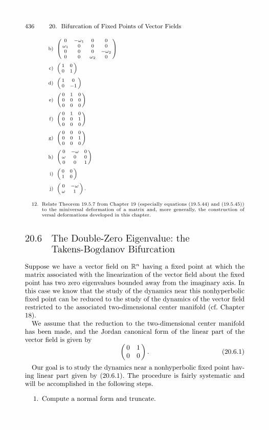
436 20. Bifurcation of Fixed Points of Vector Fields
b)
0 −ω1 0 0ω1 0 0 00 0 0 −ω20 0 ω2 0
c)(
1 00 1
)
d)(
1 00 −1
)
e)
( 0 1 00 0 00 0 0
)
f)
( 0 1 00 0 10 0 0
)
g)
( 0 0 00 0 10 0 0
)
h)
( 0 −ω 0ω 0 00 0 1
)
i)(
0 01 0
)
j)(
0 −ωω 1
).
12. Relate Theorem 19.5.7 from Chapter 19 (especially equations (19.5.44) and (19.5.45))to the miniversal deformation of a matrix and, more generally, the construction ofversal deformations developed in this chapter.
20.6 The Double-Zero Eigenvalue: theTakens-Bogdanov Bifurcation
Suppose we have a vector field on Rn having a fixed point at which the
matrix associated with the linearization of the vector field about the fixedpoint has two zero eigenvalues bounded away from the imaginary axis. Inthis case we know that the study of the dynamics near this nonhyperbolicfixed point can be reduced to the study of the dynamics of the vector fieldrestricted to the associated two-dimensional center manifold (cf. Chapter18).
We assume that the reduction to the two-dimensional center manifoldhas been made, and the Jordan canonical form of the linear part of thevector field is given by (
0 10 0
). (20.6.1)
Our goal is to study the dynamics near a nonhyperbolic fixed point hav-ing linear part given by (20.6.1). The procedure is fairly systematic andwill be accomplished in the following steps.
1. Compute a normal form and truncate.
20.6 The Double-Zero Eigenvalue: the Takens-Bogdanov Bifurcation 437
2. Rescale the normal form so as to reduce the number of cases to bestudied.
3. Embed the truncated normal form in an appropriate two-parameterfamily (see Example 20.4.11b)
4. Study the local dynamics of the two-parameter family of vector fields.
4a. Find the fixed points and study the nature of their stability.4b. Study the bifurcations associated with the fixed points.4c. Based on a consideration of the local dynamics, infer if global
bifurcations must be present.
5. Analyze the global bifurcations.
6. Study the effect of the neglected higher order terms in the normalform on the dynamics of the truncated normal form.
We remark that Step 4c is a new phenomenon. However, we will see thatit is not uncommon for global effects to be associated with local codimensionk (k ≥ 2) bifurcations. Moreover, we will see that it is often possible to“guess” their existence from a thorough local analysis. We will discuss thisin more detail later on. Now we begin our analysis with Step 1.
Step 1: The Normal Form. In Example 19.1.2 we saw that a normal formassociated with a fixed point of a vector field having linear part (20.6.1) isgiven by
x = y +O(|x|3, |y|3),y = ax2 + bxy +O(|x|3, |y|3), (x, y) ∈ R
2. (20.6.2)
At this stage we will neglect the O(3) terms in (20.6.2) and study theresulting truncated normal form
x = y,
y = ax2 + bxy. (20.6.3)
Step 2: Rescaling. Letting
x→ αx,
y → βy,
t→ γt, γ > 0,
(20.6.3) becomes
x =(
γβ
α
)y,
y =(
γaα2
β
)x2 + (γbα)xy. (20.6.4)
438 20. Bifurcation of Fixed Points of Vector Fields
Now we want to choose γ, β, and α so that the coefficients of (20.6.4) areas simple as possible. Ideally, they would all be unity; we will see that thisis not possible but that we can come close.
We will requireγβ
α= 1 (20.6.5)
orγ =
α
β.
Equation (20.6.5) fixes γ. We require α and β to have the same signs sothat stability will not be affected under the rescaling (since γ scales time).
Next, we require thatγaα2
β= 1. (20.6.6)
Using (20.6.5), (20.6.6) becomes
aα3
β2 = aα
(α2
β2
)= 1. (20.6.7)
Equation (20.6.7) fixes α/β.We finally require
γbα = 1 (20.6.8)
but, using (20.6.5), (20.6.8) becomes
bα2
β= bβ
(α2
β2
)= 1. (20.6.9)
We can see that a and b can have either sign and that α and β musthave the same sign. From (20.6.7) we can further see that a and α musthave the same sign. Therefore, if (20.6.9) is to hold, we conclude that b anda have the same sign. This is too restrictive—the best we can do and stillretain full generality is to require
bβ
(α2
β2
)= ±1, (20.6.10)
so that, in the rescaled variables, the normal form is
x = y,
y = x2 ± xy. (20.6.11)
Step 3: Construct a Candidate for a Versal Deformation. From Example20.4.11b, a likely candidate for a versal deformation is
x = y,
y = µ1 + µ2y + x2 + bxy, b = ±1. (20.6.12)
20.6 The Double-Zero Eigenvalue: the Takens-Bogdanov Bifurcation 439
Step 4: Study the Local Dynamics of (20.6.12). We take the case b = +1.
Step 4a: Fixed Points and Their Stability. It is easy to see that the fixedpoints of (20.6.12) are given by
(x, y) = (±√−µ1, 0). (20.6.13)
In particular, there are no fixed points for µ1 > 0.Next we check the stability of these fixed points.The Jacobian of the vector field evaluated at the fixed point is given by(
0 12x µ2 + x
)∣∣∣∣(±√−µ1,0)
=(
0 1±2√−µ1 µ2 ±
√−µ1
). (20.6.14)
The eigenvalues are given by
λ1,2 =µ2 ±
√−µ1
2± 1
2
√(µ2 ±
√−µ1)2 ± 8
√−µ1. (20.6.15)
If we denote the two branches of fixed points by (x+, 0) ≡ (+√−µ1, 0)
and (x−, 0) = (−√−µ1, 0), we see from (20.6.15) that (x+, 0) is a saddle
for µ1 < 0 and all µ2, while for µ1 = 0 the eigenvalues of (x+, 0) are givenby
λ1,2 = µ2, 0.
The fixed point (x−, 0) is a source for µ2 >√−µ1, µ1 < 0 and a sink for
µ2 <√−µ1, µ1 < 0; for µ1 = 0, the eigenvalues of (x−, 0) are given by
λ1,2 = µ2, 0
and, for µ2 =√−µ1, µ1 < 0, the eigenvalues on (x−, 0) are given by
λ1,2 = ± i
√2√−µ1.
Thus, we might expect that µ1 = 0 is a bifurcation curve on which (x±, 0)are born in a saddle-node bifurcation and µ2 =
√−µ1, µ1 < 0, is a bi-furcation curve on which (x−, 0) undergoes a Poincare–Andronov–Hopf bi-furcation. We now turn to verifying this and studying the orbit structureassociated with these bifurcations.
Step 4b: The Bifurcations of the Fixed Points. We begin by examining theorbit structure near µ1 = 0, µ2 arbitrary. We will use the center manifoldtheorem (Theorem 18.1.2).
First we put the system into the “normal form” for the center manifoldtheorem. We treat µ2 as a fixed constant in the problem and think of µ1as a parameter, and we examine bifurcations from µ1 = 0.
To transform (20.6.12) into the form in which the center manifold canbe applied, we use the following linear transformation(
xy
)=
(1 10 µ2
)(uv
),
(uv
)=
1µ2
(µ2 −10 1
)(xy
), (20.6.16)
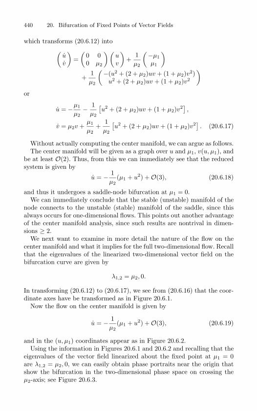
440 20. Bifurcation of Fixed Points of Vector Fields
which transforms (20.6.12) into(uv
)=
(0 00 µ2
)(uv
)+
1µ2
(−µ1µ1
)
+1µ2
(−(u2 + (2 + µ2)uv + (1 + µ2)v2)
u2 + (2 + µ2)uv + (1 + µ2)v2
)or
u = −µ1
µ2− 1
µ2
[u2 + (2 + µ2)uv + (1 + µ2)v2] ,
v = µ2v +µ1
µ2+
1µ2
[u2 + (2 + µ2)uv + (1 + µ2)v2] . (20.6.17)
Without actually computing the center manifold, we can argue as follows.The center manifold will be given as a graph over u and µ1, v(u, µ1), and
be at least O(2). Thus, from this we can immediately see that the reducedsystem is given by
u = − 1µ2
(µ1 + u2) +O(3), (20.6.18)
and thus it undergoes a saddle-node bifurcation at µ1 = 0.We can immediately conclude that the stable (unstable) manifold of the
node connects to the unstable (stable) manifold of the saddle, since thisalways occurs for one-dimensional flows. This points out another advantageof the center manifold analysis, since such results are nontrival in dimen-sions ≥ 2.
We next want to examine in more detail the nature of the flow on thecenter manifold and what it implies for the full two-dimensional flow. Recallthat the eigenvalues of the linearized two-dimensional vector field on thebifurcation curve are given by
λ1,2 = µ2, 0.
In transforming (20.6.12) to (20.6.17), we see from (20.6.16) that the coor-dinate axes have be transformed as in Figure 20.6.1.
Now the flow on the center manifold is given by
u = − 1µ2
(µ1 + u2) +O(3), (20.6.19)
and in the (u, µ1) coordinates appear as in Figure 20.6.2.Using the information in Figures 20.6.1 and 20.6.2 and recalling that the
eigenvalues of the vector field linearized about the fixed point at µ1 = 0are λ1,2 = µ2, 0, we can easily obtain phase portraits near the origin thatshow the bifurcation in the two-dimensional phase space on crossing theµ2-axis; see Figure 20.6.3.
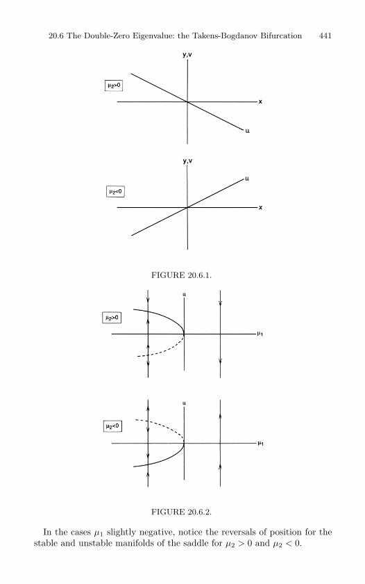
20.6 The Double-Zero Eigenvalue: the Takens-Bogdanov Bifurcation 441
FIGURE 20.6.1.
FIGURE 20.6.2.
In the cases µ1 slightly negative, notice the reversals of position for thestable and unstable manifolds of the saddle for µ2 > 0 and µ2 < 0.
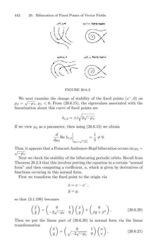
442 20. Bifurcation of Fixed Points of Vector Fields
FIGURE 20.6.3.
We next examine the change of stability of the fixed points (x−, 0) onµ2 =
√−µ1, µ1 < 0. From (20.6.15), the eigenvalues associated with thelinearization about this curve of fixed points are
λ1,2 = ±i
√2√−µ1.
If we view µ2 as a parameter, then using (20.6.15) we obtain
d
dµ2Re λ1,2
∣∣∣∣µ2=
√−µ1
=12 = 0.
Thus, it appears that a Poincare-Andronov-Hopf bifurcation occurs on µ2 =√−µ1.Next we check the stability of the bifurcating periodic orbits. Recall from
Theorem 20.2.3 that this involves putting the equation in a certain “normalform” and then computing a coefficient, a, which is given by derivatives offunctions occuring in this normal form.
First we transform the fixed point to the origin via
x = x− x−,
y = y,
so that (3.1.198) becomes(˙x˙y
)=
(0 1
−2√−µ1 0
)(xy
)+
(0
xy + x2
). (20.6.20)
Then we put the linear part of (20.6.20) in normal form via the lineartransformation (
xy
)=
(0 1√
−2√−µ1 0
)(uv
), (20.6.21)
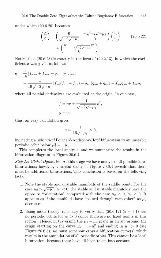
20.6 The Double-Zero Eigenvalue: the Takens-Bogdanov Bifurcation 443
under which (20.6.20) becomes(uv
)=
(0 −
√−2√−µ1√
−2√−µ1 0
)(uv
)(20.6.22)
+(
uv + 1√−2
√−µ1v2
0
).
Notice that (20.6.23) is exactly in the form of (20.2.13), in which the coef-ficient a was given as follows
a =116
[fuuu + fuvv + guuv + gvvv]
+1
16√−2√−µ1
[fuv(fuu + fvv)− guv(guu + gvv)− fuuguu + fvvgvv] ,
where all partial derivatives are evaluated at the origin. In our case,
f = uv +1√
−2√−µ1
v2,
g = 0;
thus, an easy calculation gives
a =1
16√−µ1
> 0,
indicating a subcritical Poincare-Andronov-Hopf bifurcation to an unstableperiodic orbit below µ2
2 = −µ1.This completes the local analysis, and we summarize the results in the
bifurcation diagram in Figure 20.6.4.
Step 4c: Global Dynamics. At this stage we have analyzed all possible localbifurcations; however, a careful study of Figure 20.6.4 reveals that theremust be additional bifurcations. This conclusion is based on the followingfacts.
1. Note the stable and unstable manifolds of the saddle point. For thecase µ2 >
√−µ1, µ1 < 0, the stable and unstable manifolds have theopposite “orientation” compared with the case µ2 < 0, µ1 < 0. Itappears as if the manifolds have “passed through each other” as µ2decreases.
2. Using index theory, it is easy to verify that (20.6.12) (b = +1) hasno periodic orbits for µ1 > 0 (since there are no fixed points in thisregion). Hence, in traversing the µ1 − µ2 plane in an arc around theorigin starting on the curve µ2 = −µ2
1 and ending in µ1 > 0 (seeFigure 20.6.5), we must somehow cross a bifurcation curve(s) whichresults in the annihilation of all periodic orbits. This cannot be a localbifurcation, because these have all been taken into account.
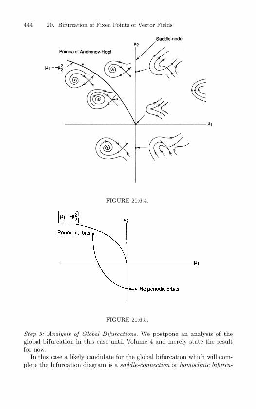
444 20. Bifurcation of Fixed Points of Vector Fields
FIGURE 20.6.4.
FIGURE 20.6.5.
Step 5: Analysis of Global Bifurcations. We postpone an analysis of theglobal bifurcation in this case until Volume 4 and merely state the resultfor now.
In this case a likely candidate for the global bifurcation which will com-plete the bifurcation diagram is a saddle-connection or homoclinic bifurca-
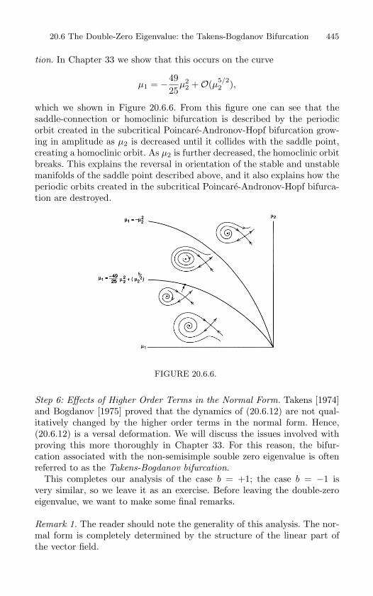
20.6 The Double-Zero Eigenvalue: the Takens-Bogdanov Bifurcation 445
tion. In Chapter 33 we show that this occurs on the curve
µ1 = −4925
µ22 +O(µ5/2
2 ),
which we shown in Figure 20.6.6. From this figure one can see that thesaddle-connection or homoclinic bifurcation is described by the periodicorbit created in the subcritical Poincare-Andronov-Hopf bifurcation grow-ing in amplitude as µ2 is decreased until it collides with the saddle point,creating a homoclinic orbit. As µ2 is further decreased, the homoclinic orbitbreaks. This explains the reversal in orientation of the stable and unstablemanifolds of the saddle point described above, and it also explains how theperiodic orbits created in the subcritical Poincare-Andronov-Hopf bifurca-tion are destroyed.
FIGURE 20.6.6.
Step 6: Effects of Higher Order Terms in the Normal Form. Takens [1974]and Bogdanov [1975] proved that the dynamics of (20.6.12) are not qual-itatively changed by the higher order terms in the normal form. Hence,(20.6.12) is a versal deformation. We will discuss the issues involved withproving this more thoroughly in Chapter 33. For this reason, the bifur-cation associated with the non-semisimple souble zero eigenvalue is oftenreferred to as the Takens-Bogdanov bifurcation.
This completes our analysis of the case b = +1; the case b = −1 isvery similar, so we leave it as an exercise. Before leaving the double-zeroeigenvalue, we want to make some final remarks.
Remark 1. The reader should note the generality of this analysis. The nor-mal form is completely determined by the structure of the linear part ofthe vector field.
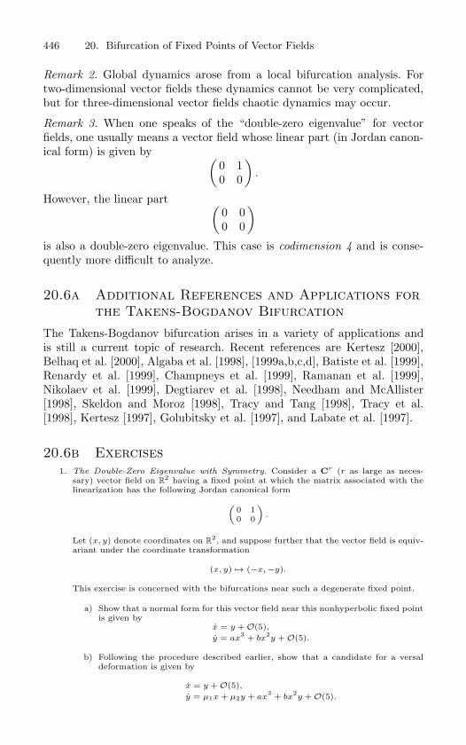
446 20. Bifurcation of Fixed Points of Vector Fields
Remark 2. Global dynamics arose from a local bifurcation analysis. Fortwo-dimensional vector fields these dynamics cannot be very complicated,but for three-dimensional vector fields chaotic dynamics may occur.
Remark 3. When one speaks of the “double-zero eigenvalue” for vectorfields, one usually means a vector field whose linear part (in Jordan canon-ical form) is given by (
0 10 0
).
However, the linear part (0 00 0
)is also a double-zero eigenvalue. This case is codimension 4 and is conse-quently more difficult to analyze.
20.6a Additional References and Applications forthe Takens-Bogdanov Bifurcation
The Takens-Bogdanov bifurcation arises in a variety of applications andis still a current topic of research. Recent references are Kertesz [2000],Belhaq et al. [2000], Algaba et al. [1998], [1999a,b,c,d], Batiste et al. [1999],Renardy et al. [1999], Champneys et al. [1999], Ramanan et al. [1999],Nikolaev et al. [1999], Degtiarev et al. [1998], Needham and McAllister[1998], Skeldon and Moroz [1998], Tracy and Tang [1998], Tracy et al.[1998], Kertesz [1997], Golubitsky et al. [1997], and Labate et al. [1997].
20.6b Exercises1. The Double-Zero Eigenvalue with Symmetry. Consider a Cr (r as large as neces-
sary) vector field on R2 having a fixed point at which the matrix associated with the
linearization has the following Jordan canonical form
(0 10 0
).
Let (x, y) denote coordinates on R2, and suppose further that the vector field is equiv-
ariant under the coordinate transformation
(x, y) → (−x, −y).
This exercise is concerned with the bifurcations near such a degenerate fixed point.
a) Show that a normal form for this vector field near this nonhyperbolic fixed pointis given by
x = y + O(5),y = ax
3 + bx2y + O(5).
b) Following the procedure described earlier, show that a candidate for a versaldeformation is given by
x = y + O(5),y = µ1x + µ2y + ax
3 + bx2y + O(5).
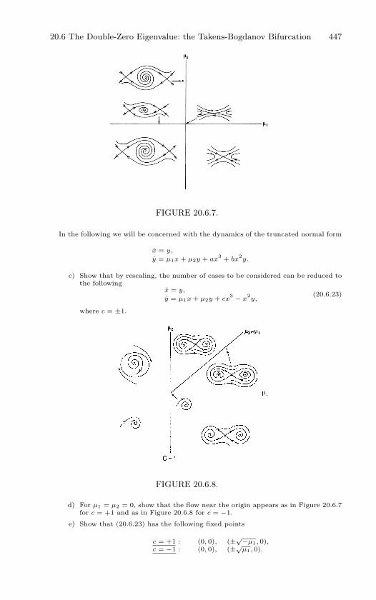
20.6 The Double-Zero Eigenvalue: the Takens-Bogdanov Bifurcation 447
FIGURE 20.6.7.
In the following we will be concerned with the dynamics of the truncated normal form
x = y,
y = µ1x + µ2y + ax3 + bx
2y.
c) Show that by rescaling, the number of cases to be considered can be reduced tothe following
x = y,
y = µ1x + µ2y + cx3 − x
2y,
(20.6.23)
where c = ±1.
FIGURE 20.6.8.
d) For µ1 = µ2 = 0, show that the flow near the origin appears as in Figure 20.6.7for c = +1 and as in Figure 20.6.8 for c = −1.
e) Show that (20.6.23) has the following fixed points
c = +1 : (0, 0), (±√−µ1, 0),c = −1 : (0, 0), (±√
µ1, 0).
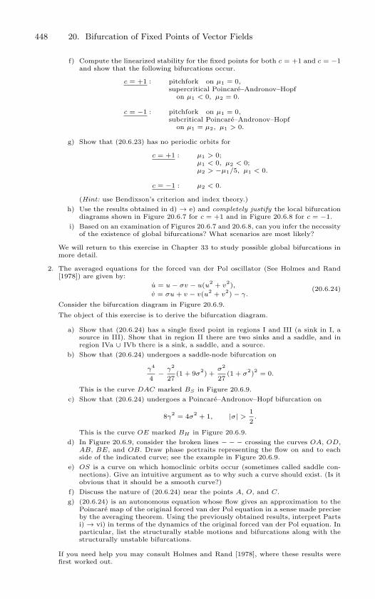
448 20. Bifurcation of Fixed Points of Vector Fields
f) Compute the linearized stability for the fixed points for both c = +1 and c = −1and show that the following bifurcations occur.
c = +1 : pitchfork on µ1 = 0,supercritical Poincare–Andronov–Hopf
on µ1 < 0, µ2 = 0.
c = −1 : pitchfork on µ1 = 0,subcritical Poincare–Andronov–Hopf
on µ1 = µ2, µ1 > 0.
g) Show that (20.6.23) has no periodic orbits for
c = +1 : µ1 > 0;µ1 < 0, µ2 < 0;µ2 > −µ1/5, µ1 < 0.
c = −1 : µ2 < 0.
(Hint: use Bendixson’s criterion and index theory.)h) Use the results obtained in d) → e) and completely justify the local bifurcation
diagrams shown in Figure 20.6.7 for c = +1 and in Figure 20.6.8 for c = −1.i) Based on an examination of Figures 20.6.7 and 20.6.8, can you infer the necessity
of the existence of global bifurcations? What scenarios are most likely?
We will return to this exercise in Chapter 33 to study possible global bifurcations inmore detail.
2. The averaged equations for the forced van der Pol oscillator (See Holmes and Rand[1978]) are given by:
u = u − σv − u(u2 + v2),
v = σu + v − v(u2 + v2) − γ.
(20.6.24)
Consider the bifurcation diagram in Figure 20.6.9.
The object of this exercise is to derive the bifurcation diagram.
a) Show that (20.6.24) has a single fixed point in regions I and III (a sink in I, asource in III). Show that in region II there are two sinks and a saddle, and inregion IVa ∪ IVb there is a sink, a saddle, and a source.
b) Show that (20.6.24) undergoes a saddle-node bifurcation on
γ4
4− γ2
27(1 + 9σ
2) +σ2
27(1 + σ
2)2 = 0.
This is the curve DAC marked BS in Figure 20.6.9.c) Show that (20.6.24) undergoes a Poincare–Andronov–Hopf bifurcation on
8γ2 = 4σ
2 + 1, |σ| >12
.
This is the curve OE marked BH in Figure 20.6.9.d) In Figure 20.6.9, consider the broken lines − − − crossing the curves OA, OD,
AB, BE, and OB. Draw phase portraits representing the flow on and to eachside of the indicated curve; see the example in Figure 20.6.9.
e) OS is a curve on which homoclinic orbits occur (sometimes called saddle con-nections). Give an intuitive argument as to why such a curve should exist. (Is itobvious that it should be a smooth curve?)
f) Discuss the nature of (20.6.24) near the points A, O, and C.g) (20.6.24) is an autonomous equation whose flow gives an approximation to the
Poincare map of the original forced van der Pol equation in a sense made preciseby the averaging theorem. Using the previously obtained results, interpret Partsi) → vi) in terms of the dynamics of the original forced van der Pol equation. Inparticular, list the structurally stable motions and bifurcations along with thestructurally unstable bifurcations.
If you need help you may consult Holmes and Rand [1978], where these results werefirst worked out.
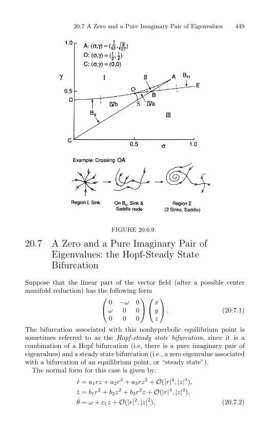
20.7 A Zero and a Pure Imaginary Pair of Eigenvalues 449
FIGURE 20.6.9.
20.7 A Zero and a Pure Imaginary Pair ofEigenvalues: the Hopf-Steady StateBifurcation
Suppose that the linear part of the vector field (after a possible centermanifold reduction) has the following form
0 −ω 0ω 0 00 0 0
x
yz
. (20.7.1)
The bifurcation associated with this nonhyperbolic equilibrium point issometimes referred to as the Hopf-steady state bifurcation, since it is acombination of a Hopf bifurcation (i.e, there is a pure imaginary pair ofeigenvalues) and a steady state bifurcation (i.e., a zero eigenvalue associatedwith a bifurcation of an equilibrium point, or “steady state”).
The normal form for this case is given by:
r = a1rz + a2r3 + a3rz
2 +O(|r|4, |z|4),z = b1r
2 + b2z2 + b3r
2z +O(|r|4, |z|4),θ = ω + c1z +O(|r|2, |z|2), (20.7.2)
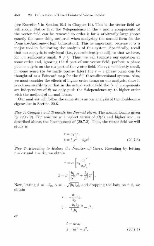
450 20. Bifurcation of Fixed Points of Vector Fields
(see Exercise 5 in Section 19.4 in Chapter 19). This is the vector field wewill study. Notice that the θ-dependence in the r and z components ofthe vector field can be removed to order k for k arbitrarily large (note:exactly the same thing occurred when analyzing the normal form for thePoincare-Andronov-Hopf bifurcation). This is important. because it is amajor tool in facilitating the analysis of this system. Specifically, recallthat our analysis is only local (i.e., r, z sufficiently small), so that we have,for r, z sufficiently small, θ = 0. Thus, we will truncate our equation atsome order and, ignoring the θ part of our vector field, perform a phaseplane analysis on the r, z part of the vector field. For r, z sufficiently small,in some sense (to be made precise later) the r − z phase plane can bethought of as a Poincare map for the full three-dimensional system. Also,we must consider the effects of higher order terms on our analysis, since itis not necessarily true that in the actual vector field the (r, z) componentsare independent of θ; we only push the θ-dependence up to higher orderwith the method of normal forms.
Our analysis will follow the same steps as our analysis of the double-zeroeigenvalue in Section 20.6.
Step 1: Compute and Truncate the Normal Form. The normal form is givenby (20.7.2). For now we will neglect terms of O(3) and higher and, asdescribed above, the θ component of (20.7.2). Thus, the vector field we willstudy is
r = a1rz,
z = b1r2 + b2z
2. (20.7.3)
Step 2: Rescaling to Reduce the Number of Cases. Rescaling by lettingr = αr and z = βz, we obtain
˙r = α
[a1
rz
αβ
],
˙z = β
[b1
α2 r2 +b2
β2 z2]
.
Now, letting β = −b2, α = −√|b1b2|, and dropping the bars on r, z, we
obtain
r = −a1
b2rz,
z =−b1b2
|b1b2|r2 − z2,
or
r = arz,
z = br2 − z2, (20.7.4)
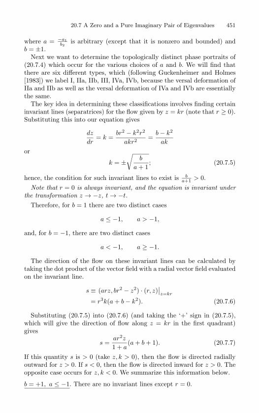
20.7 A Zero and a Pure Imaginary Pair of Eigenvalues 451
where a = −a1b2
is arbitrary (except that it is nonzero and bounded) andb = ±1.
Next we want to determine the topologically distinct phase portraits of(20.7.4) which occur for the various choices of a and b. We will find thatthere are six different types, which (following Guckenheimer and Holmes[1983]) we label I, IIa, IIb, III, IVa, IVb, because the versal deformation ofIIa and IIb as well as the versal deformation of IVa and IVb are essentiallythe same.
The key idea in determining these classifications involves finding certaininvariant lines (separatrices) for the flow given by z = kr (note that r ≥ 0).Substituting this into our equation gives
dz
dr= k =
br2 − k2r2
akr2 =b− k2
ak
or
k = ±√
b
a + 1; (20.7.5)
hence, the condition for such invariant lines to exist is ba+1 > 0.
Note that r = 0 is always invariant, and the equation is invariant under
the transformation z → −z, t → −t.
Therefore, for b = 1 there are two distinct cases
a ≤ −1, a > −1,
and, for b = −1, there are two distinct cases
a < −1, a ≥ −1.
The direction of the flow on these invariant lines can be calculated bytaking the dot product of the vector field with a radial vector field evaluatedon the invariant line.
s ≡ (arz, br2 − z2) · (r, z)∣∣z=kr
= r3k(a + b− k2). (20.7.6)
Substituting (20.7.5) into (20.7.6) (and taking the ‘+’ sign in (20.7.5),which will give the direction of flow along z = kr in the first quadrant)gives
s =ar2z
1 + a(a + b + 1). (20.7.7)
If this quantity s is > 0 (take z, k > 0), then the flow is directed radiallyoutward for z > 0. If s < 0, then the flow is directed inward for z > 0. Theopposite case occurs for z, k < 0. We summarize this information below.
b = +1, a ≤ −1. There are no invariant lines except r = 0.
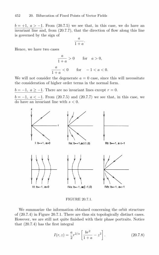
452 20. Bifurcation of Fixed Points of Vector Fields
b = +1, a > −1. From (20.7.5) we see that, in this case, we do have aninvariant line and, from (20.7.7), that the direction of flow along this lineis governed by the sign of
a
1 + a.
Hence, we have two cases
a
1 + a> 0 for a > 0,
a
1 + a< 0 for − 1 < a < 0.
We will not consider the degenerate a = 0 case, since this will necessitatethe consideration of higher order terms in the normal form.
b = −1, a ≥ −1. There are no invariant lines except r = 0.
b = −1, a < −1. From (20.7.5) and (20.7.7) we see that, in this case, wedo have an invariant line with s < 0.
FIGURE 20.7.1.
We summarize the information obtained concerning the orbit structureof (20.7.4) in Figure 20.7.1. There are thus six topologically distinct cases.However, we are still not quite finished with their phase portraits. Noticethat (20.7.4) has the first integral
I(r, z) =a
2r2/a
[br2
1 + a− z2
]. (20.7.8)
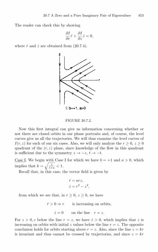
20.7 A Zero and a Pure Imaginary Pair of Eigenvalues 453
The reader can check this by showing
∂I
∂rr +
∂I
∂zz = 0,
where r and z are obtained from (20.7.4).
FIGURE 20.7.2.
Now this first integral can give us information concerning whether ornot there are closed orbits in our phase portraits and, of course, the levelcurves give us all the trajectories. We will thus examine the level curves ofI(r, z) for each of our six cases. Also, we will only analyze the r ≥ 0, z ≥ 0quadrant of the (r, z) plane, since knowledge of the flow in this quadrantis sufficient due to the symmetry z → −z, t → −t.
Case I. We begin with Case I for which we have b = +1 and a > 0, whichimplies that k =
√1
1+a < 1.Recall that, in this case, the vector field is given by
r = arz,
z = r2 − z2,
from which we see that, in r ≥ 0, z ≥ 0, we have
r > 0 ⇒ r is increasing on orbits,
z = 0 on the line r = z.
For z > 0, z below the line r = z, we have z > 0, which implies that z isincreasing on orbits with initial z values below the line r = z. The oppositeconclusion holds for orbits starting above r = z. Also, since the line z = kris invariant and thus cannot be crossed by trajectories, and since z = kr
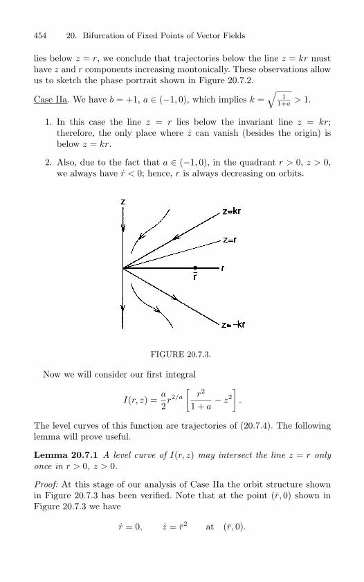
454 20. Bifurcation of Fixed Points of Vector Fields
lies below z = r, we conclude that trajectories below the line z = kr musthave z and r components increasing montonically. These observations allowus to sketch the phase portrait shown in Figure 20.7.2.
Case IIa. We have b = +1, a ∈ (−1, 0), which implies k =√
11+a > 1.
1. In this case the line z = r lies below the invariant line z = kr;therefore, the only place where z can vanish (besides the origin) isbelow z = kr.
2. Also, due to the fact that a ∈ (−1, 0), in the quadrant r > 0, z > 0,we always have r < 0; hence, r is always decreasing on orbits.
FIGURE 20.7.3.
Now we will consider our first integral
I(r, z) =a
2r2/a
[r2
1 + a− z2
].
The level curves of this function are trajectories of (20.7.4). The followinglemma will prove useful.
Lemma 20.7.1 A level curve of I(r, z) may intersect the line z = r only
once in r > 0, z > 0.
Proof: At this stage of our analysis of Case IIa the orbit structure shownin Figure 20.7.3 has been verified. Note that at the point (r, 0) shown inFigure 20.7.3 we have
r = 0, z = r2 at (r, 0).
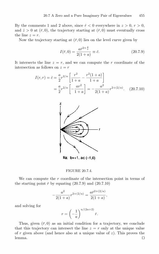
20.7 A Zero and a Pure Imaginary Pair of Eigenvalues 455
By the comments 1 and 2 above, since r < 0 everywhere in z > 0, r > 0,and z > 0 at (r, 0), the trajectory starting at (r, 0) must eventually crossthe line z = r.
Now the trajectory starting at (r, 0) lies on the level curve given by
I(r, 0) =ar2+ 2
a
2(1 + a)≡ c. (20.7.9)
It intersects the line z = r, and we can compute the r coordinate of theintersection as follows on z = r
I(r, r) = c =a
2r2/a
[r2
1 + a− r2(1 + a)
1 + a
]
=a
2r2/a
[− ar2
1 + a
]= − a2
2(1 + a)r2+(2/a). (20.7.10)
FIGURE 20.7.4.
We can compute the r coordinate of the intersection point in terms ofthe starting point r by equating (20.7.9) and (20.7.10)
− a2
2(1 + a)r2+(2/a) =
ar2+(2/a)
2(1 + a),
and solving for
r =(−1
a
)a/(2a+2)
r.
Thus, given (r, 0) as an initial condition for a trajectory, we concludethat this trajectory can intersect the line z = r only at the unique valueof r given above (and hence also at a unique value of z). This proves thelemma.
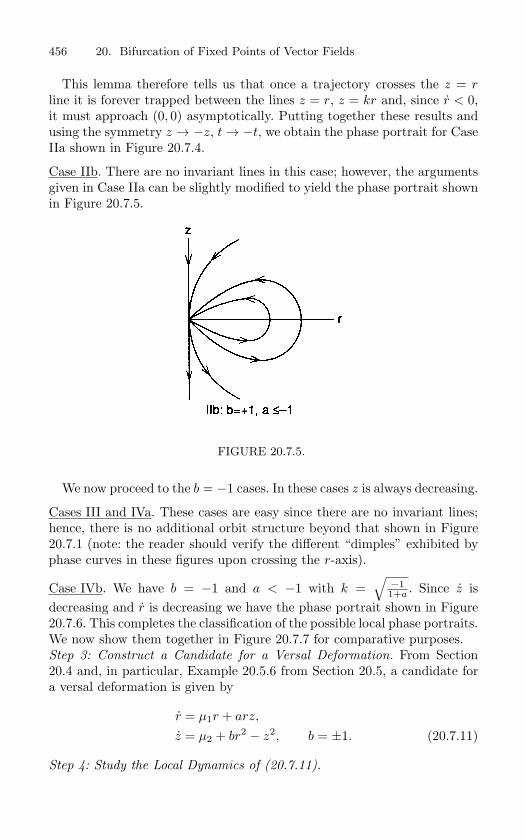
456 20. Bifurcation of Fixed Points of Vector Fields
This lemma therefore tells us that once a trajectory crosses the z = rline it is forever trapped between the lines z = r, z = kr and, since r < 0,it must approach (0, 0) asymptotically. Putting together these results andusing the symmetry z → −z, t → −t, we obtain the phase portrait for CaseIIa shown in Figure 20.7.4.
Case IIb. There are no invariant lines in this case; however, the argumentsgiven in Case IIa can be slightly modified to yield the phase portrait shownin Figure 20.7.5.
FIGURE 20.7.5.
We now proceed to the b = −1 cases. In these cases z is always decreasing.
Cases III and IVa. These cases are easy since there are no invariant lines;hence, there is no additional orbit structure beyond that shown in Figure20.7.1 (note: the reader should verify the different “dimples” exhibited byphase curves in these figures upon crossing the r-axis).
Case IVb. We have b = −1 and a < −1 with k =√
−11+a . Since z is
decreasing and r is decreasing we have the phase portrait shown in Figure20.7.6. This completes the classification of the possible local phase portraits.We now show them together in Figure 20.7.7 for comparative purposes.Step 3: Construct a Candidate for a Versal Deformation. From Section20.4 and, in particular, Example 20.5.6 from Section 20.5, a candidate fora versal deformation is given by
r = µ1r + arz,
z = µ2 + br2 − z2, b = ±1. (20.7.11)
Step 4: Study the Local Dynamics of (20.7.11).
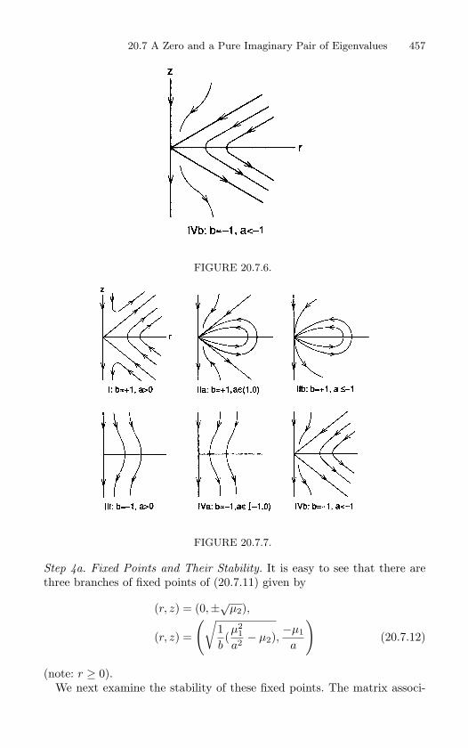
20.7 A Zero and a Pure Imaginary Pair of Eigenvalues 457
FIGURE 20.7.6.
FIGURE 20.7.7.
Step 4a. Fixed Points and Their Stability. It is easy to see that there arethree branches of fixed points of (20.7.11) given by
(r, z) = (0,±√µ2),
(r, z) =
(√1b(µ2
1
a2 − µ2),−µ1
a
)(20.7.12)
(note: r ≥ 0).We next examine the stability of these fixed points. The matrix associ-
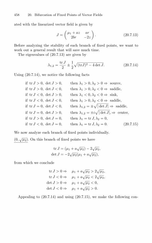
458 20. Bifurcation of Fixed Points of Vector Fields
ated with the linearized vector field is given by
J =(
µ1 + az ar2br −2z
). (20.7.13)
Before analyzing the stability of each branch of fixed points, we want towork out a general result that will save much time.
The eigenvalues of (20.7.13) are given by
λ1,2 =trJ
2± 1
2
√(trJ)2 − 4 det J. (20.7.14)
Using (20.7.14), we notice the following facts
if trJ > 0, det J > 0, then λ1 > 0, λ2 > 0 ⇒ source,if trJ > 0, det J < 0, then λ1 > 0, λ2 < 0 ⇒ saddle,if trJ < 0, det J > 0, then λ1 < 0, λ2 < 0 ⇒ sink,if trJ < 0, det J < 0, then λ1 > 0, λ2 < 0 ⇒ saddle,if trJ = 0, det J < 0, then λ1,2 = ±
√|det J | ⇒ saddle,
if trJ = 0, det J > 0, then λ1,2 = ±i√| detJ |,⇒ center,
if trJ > 0, det J = 0, then λ1 = trJ, λ2 = 0,
if trJ < 0, det J = 0, then λ1 = trJ, λ2 = 0. (20.7.15)
We now analyze each branch of fixed points individually.
(0,√
µ2). On this branch of fixed points we have
trJ = (µ1 + a√
µ2)− 2√
µ2,
det J = −2√
µ2(µ1 + a√
µ2),
from which we conclude
trJ > 0⇒ µ1 + a√
µ2 > 2√
µ2,
trJ < 0⇒ µ1 + a√
µ2 < 2√
µ2,
det J > 0⇒ µ1 + a√
µ2 < 0,
det J < 0⇒ µ1 + a√
µ2 > 0.
Appealing to (20.7.14) and using (20.7.15), we make the following con-
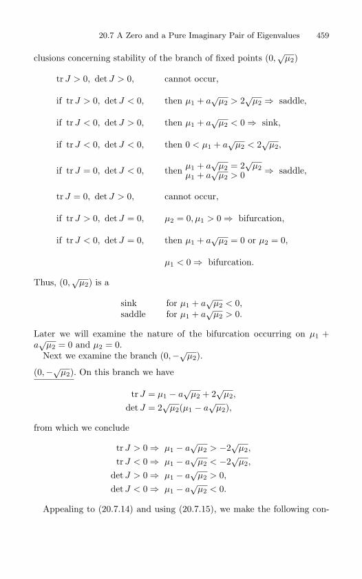
20.7 A Zero and a Pure Imaginary Pair of Eigenvalues 459
clusions concerning stability of the branch of fixed points (0,√
µ2)
trJ > 0, det J > 0, cannot occur,
if trJ > 0, det J < 0, then µ1 + a√
µ2 > 2√
µ2 ⇒ saddle,
if trJ < 0, det J > 0, then µ1 + a√
µ2 < 0 ⇒ sink,
if trJ < 0, det J < 0, then 0 < µ1 + a√
µ2 < 2√
µ2,
if trJ = 0, det J < 0, then µ1 + a√
µ2 = 2√
µ2µ1 + a
√µ2 > 0 ⇒ saddle,
trJ = 0, det J > 0, cannot occur,
if trJ > 0, det J = 0, µ2 = 0, µ1 > 0 ⇒ bifurcation,
if trJ < 0, det J = 0, then µ1 + a√
µ2 = 0 or µ2 = 0,
µ1 < 0 ⇒ bifurcation.
Thus, (0,√
µ2) is a
sink for µ1 + a√
µ2 < 0,saddle for µ1 + a
õ2 > 0.
Later we will examine the nature of the bifurcation occurring on µ1 +a√
µ2 = 0 and µ2 = 0.Next we examine the branch (0,−√µ2).
(0,−√µ2). On this branch we have
trJ = µ1 − a√
µ2 + 2√
µ2,
det J = 2√
µ2(µ1 − a√
µ2),
from which we conclude
trJ > 0⇒ µ1 − a√
µ2 > −2√
µ2,
trJ < 0⇒ µ1 − a√
µ2 < −2√
µ2,
det J > 0⇒ µ1 − a√
µ2 > 0,
det J < 0⇒ µ1 − a√
µ2 < 0.
Appealing to (20.7.14) and using (20.7.15), we make the following con-
460 20. Bifurcation of Fixed Points of Vector Fields
clusions concerning the stability of the branch of fixed points (0,−√µ2):
if trJ > 0, det J > 0, then µ1 − a√
µ2 > 0 ⇒ source,
if trJ > 0, det J < 0, then 0 > µ1 − a√
µ2 > −2√
µ2 ⇒ saddle,
trJ < 0, det J > 0, cannot occur,
if trJ < 0, det J < 0, then µ1 − a√
µ2 < −2√
µ2 ⇒ saddle,
trJ = 0, det J > 0 cannot occur,
if trJ = 0, det J < 0, then µ1 − a√
µ2 = −2√
µ2 ⇒ saddle,
if trJ > 0, det J = 0, then µ1 = a√
µ2 ⇒ bifurcation,
trJ < 0, det J = 0 cannot occur.
We thus conclude that (0,−√µ2 > 0) has the following stability character-istics.
source for µ1 − a√
µ2 > 0,saddle for µ1 − a
õ2 < 0.
Later we will examine the bifurcation occuring on µ1 − a√
µ2 = 0.Now we turn to an examination of the remaining branch of fixed points
(note that our previous analysis did not depend on b)
(r, z) =
(√1b
(µ2
1
a2 − µ2
),−µ1
a
).
We examine the cases b = +1 and b = −1 separately.
b = +1,
(õ2
1
a2 − µ2,−µ1
a
). This branch exists only for
µ21
a2 > µ2, and on
this branch we have
trJ =2µ1
a, (20.7.16)
det J = −2a
(µ2
1
a2 − µ2
). (20.7.17)
We now must consider Cases I and IIa and b individually.
Case I: a > 0. From (20.7.17), for a > 0 we have det J ≤ 0. Using (20.7.15),for detJ ≤ 0, the fixed point is always a saddle.
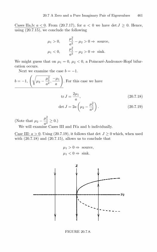
20.7 A Zero and a Pure Imaginary Pair of Eigenvalues 461
Cases IIa,b: a < 0. From (20.7.17), for a < 0 we have det J ≥ 0. Hence,using (20.7.15), we conclude the following
µ1 > 0,µ2
1
a2 − µ2 > 0⇒ source,
µ1 < 0,µ2
1
a2 − µ2 > 0⇒ sink.
We might guess that on µ1 = 0, µ2 < 0, a Poincare-Andronov-Hopf bifur-cation occurs.
Next we examine the case b = −1.
b = −1,
(√µ2 −
µ21
a2 ,−µ1
a
). For this case we have
trJ =2µ1
a, (20.7.18)
det J = 2a
(µ2 −
µ21
a2
). (20.7.19)
(Note that µ2 −µ2
1
a2 ≥ 0.)We will examine Cases III and IVa and b individually.
Case III: a > 0. Using (20.7.19), it follows that det J ≥ 0 which, when usedwith (20.7.18) and (20.7.15), allows us to conclude that
µ1 > 0⇒ source,µ1 < 0⇒ sink.
FIGURE 20.7.8.
462 20. Bifurcation of Fixed Points of Vector Fields
Hence, we might guess that a Poincare-Andronov-Hopf bifurcation ispossible on µ1 = 0, µ2 > 0.
Cases IVa,b: a < 0. Using (20.7.19), we see that det J ≤ 0, which, whenused with (20.7.18) and (20.7.15), allows us to conclude that
µ1 < 0⇒ saddle,µ1 > 0⇒ saddle.
Hence, no Poincare-Andronov-Hopf bifurcations occur.This completes the stability analysis of the fixed points. We next examine
the nature of the various possible bifurcations.
Step 4b: The Bifurcations of the Fixed Points. First we examine the twobranches
(0,±√µ2) .
These branches exist only for µ2 ≥ 0, coalescing at µ2 = 0. We thus ex-pect them to bifurcate from (0, 0) in a saddle-node bifurcation. Since thesebranches start on r = 0 and remain on r = 0, the center manifold analysisis particulary simple—we simply set r = 0 in our original equations andobtain
z = µ2 − z2.
(Note that the equation is independent of b with bifurcation diagram shownin Figure 20.7.8.)
Next we examine the bifurcation of the branches (0,±√µ2), µ2 > 0,which occurs on µ1 ± a
õ2 = 0.
We will do a center manifold analysis. First we transform the fixed pointto the origin.
Letting ξ = z ∓√µ2, (20.7.11) becomes
r = µ1r + ar(ξ ±√µ2),
ξ = µ2 + br2 − (ξ ±√µ2)2, µ2 > 0. (20.7.20)
We are interested in the flow in a neighborhood of the curve µ1±a√
µ2 =0; we illustrate this curve in the (µ1−µ2)-parameter plane in Figure 20.7.9.
Therefore, we will set µ1 = constant and√
µ2 = ∓µ1a − ε. This corre-
sponds to crossing the parabola vertically for fixed µ1. We will have to payclose attention to the direction in which we cross the curve by varying ε;we will come back to this later. Substituting
√µ2 = ∓µ1
a − ε into (20.7.20)gives
r = µ1r + ar(ξ ±
(∓µ1
a− ε
)),
ξ =(∓µ1
a− ε
)2+ br2 −
(ξ ±
(∓µ1
a− ε
))2,
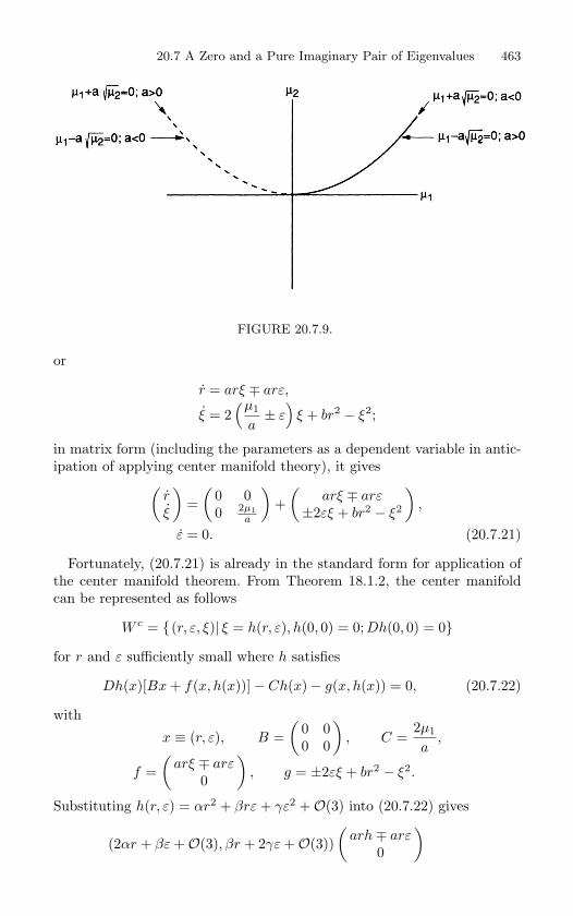
20.7 A Zero and a Pure Imaginary Pair of Eigenvalues 463
FIGURE 20.7.9.
or
r = arξ ∓ arε,
ξ = 2(µ1
a± ε
)ξ + br2 − ξ2;
in matrix form (including the parameters as a dependent variable in antic-ipation of applying center manifold theory), it gives(
rξ
)=
(0 00 2µ1
a
)+
(arξ ∓ arε
±2εξ + br2 − ξ2
),
ε = 0. (20.7.21)
Fortunately, (20.7.21) is already in the standard form for application ofthe center manifold theorem. From Theorem 18.1.2, the center manifoldcan be represented as follows
W c = (r, ε, ξ)| ξ = h(r, ε), h(0, 0) = 0;Dh(0, 0) = 0
for r and ε sufficiently small where h satisfies
Dh(x)[Bx + f(x, h(x))]− Ch(x)− g(x, h(x)) = 0, (20.7.22)
with
x ≡ (r, ε), B =(
0 00 0
), C =
2µ1
a,
f =(
arξ ∓ arε0
), g = ±2εξ + br2 − ξ2.
Substituting h(r, ε) = αr2 + βrε + γε2 +O(3) into (20.7.22) gives
(2αr + βε +O(3), βr + 2γε +O(3))(
arh∓ arε0
)
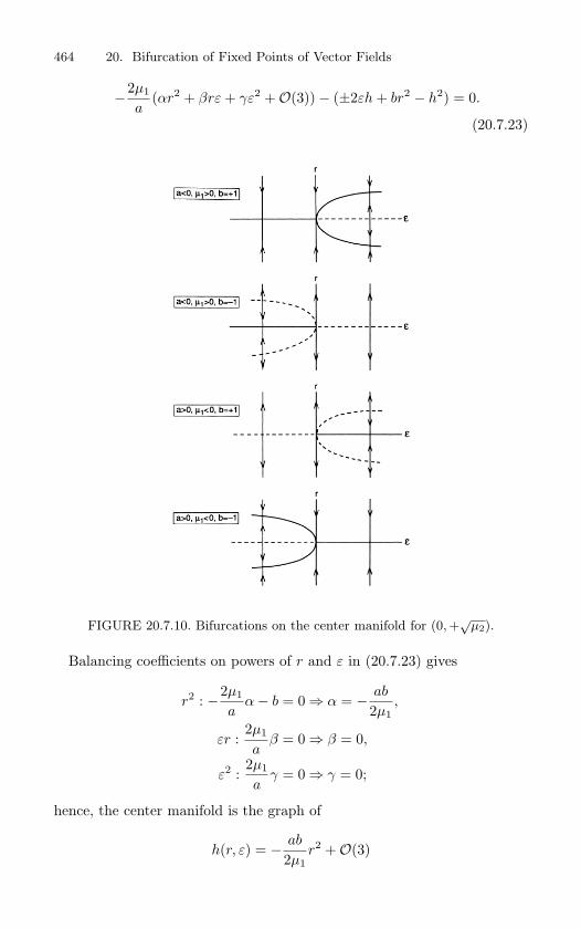
464 20. Bifurcation of Fixed Points of Vector Fields
−2µ1
a(αr2 + βrε + γε2 +O(3))− (±2εh + br2 − h2) = 0.
(20.7.23)
FIGURE 20.7.10. Bifurcations on the center manifold for (0, +√
µ2).
Balancing coefficients on powers of r and ε in (20.7.23) gives
r2 : −2µ1
aα− b = 0⇒ α = − ab
2µ1,
εr :2µ1
aβ = 0⇒ β = 0,
ε2 :2µ1
aγ = 0⇒ γ = 0;
hence, the center manifold is the graph of
h(r, ε) = − ab
2µ1r2 +O(3)
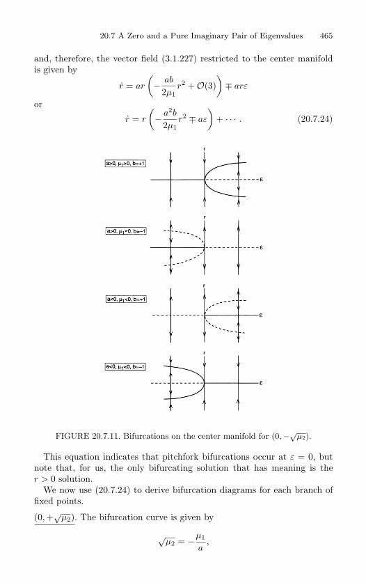
20.7 A Zero and a Pure Imaginary Pair of Eigenvalues 465
and, therefore, the vector field (3.1.227) restricted to the center manifoldis given by
r = ar
(− ab
2µ1r2 +O(3)
)∓ arε
or
r = r
(− a2b
2µ1r2 ∓ aε
)+ · · · . (20.7.24)
FIGURE 20.7.11. Bifurcations on the center manifold for (0, −√µ2).
This equation indicates that pitchfork bifurcations occur at ε = 0, butnote that, for us, the only bifurcating solution that has meaning is ther > 0 solution.
We now use (20.7.24) to derive bifurcation diagrams for each branch offixed points.
(0,+√
µ2). The bifurcation curve is given by
√µ2 = −µ1
a,
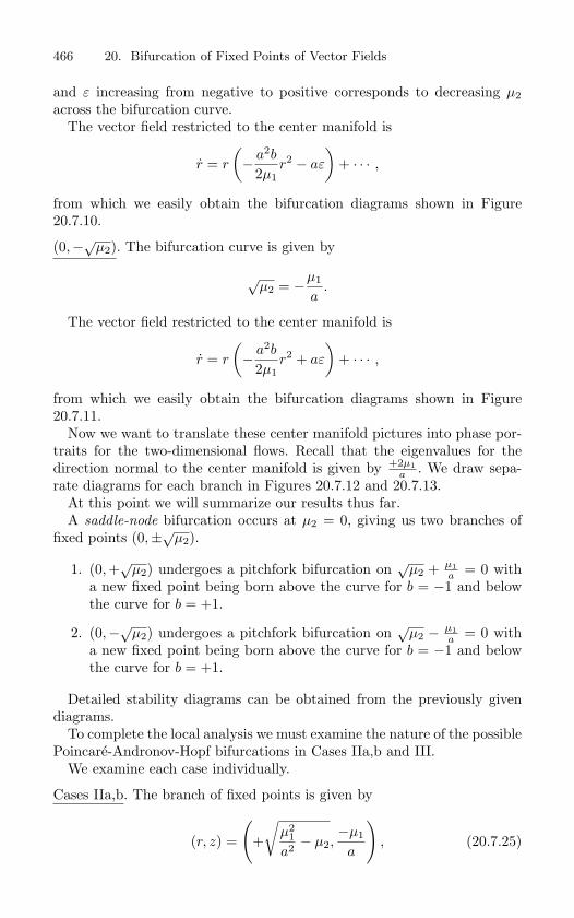
466 20. Bifurcation of Fixed Points of Vector Fields
and ε increasing from negative to positive corresponds to decreasing µ2across the bifurcation curve.
The vector field restricted to the center manifold is
r = r
(− a2b
2µ1r2 − aε
)+ · · · ,
from which we easily obtain the bifurcation diagrams shown in Figure20.7.10.
(0,−√µ2). The bifurcation curve is given by
√µ2 = −µ1
a.
The vector field restricted to the center manifold is
r = r
(− a2b
2µ1r2 + aε
)+ · · · ,
from which we easily obtain the bifurcation diagrams shown in Figure20.7.11.
Now we want to translate these center manifold pictures into phase por-traits for the two-dimensional flows. Recall that the eigenvalues for thedirection normal to the center manifold is given by +2µ1
a . We draw sepa-rate diagrams for each branch in Figures 20.7.12 and 20.7.13.
At this point we will summarize our results thus far.A saddle-node bifurcation occurs at µ2 = 0, giving us two branches of
fixed points (0,±√µ2).
1. (0, +√
µ2) undergoes a pitchfork bifurcation on√
µ2 + µ1a = 0 with
a new fixed point being born above the curve for b = −1 and belowthe curve for b = +1.
2. (0,−√µ2) undergoes a pitchfork bifurcation on√
µ2 − µ1a = 0 with
a new fixed point being born above the curve for b = −1 and belowthe curve for b = +1.
Detailed stability diagrams can be obtained from the previously givendiagrams.
To complete the local analysis we must examine the nature of the possiblePoincare-Andronov-Hopf bifurcations in Cases IIa,b and III.
We examine each case individually.
Cases IIa,b. The branch of fixed points is given by
(r, z) =
(+
õ2
1
a2 − µ2,−µ1
a
), (20.7.25)
20.7 A Zero and a Pure Imaginary Pair of Eigenvalues 467
FIGURE 20.7.12. Bifurcations in the r − ξ plane for (0, +√
µ2).
where a < 0 andµ2
1
a2 ≥ µ2.Our candidate for the Poincare-Andronov-Hopf bifurcation curve is given
byµ1 = 0, µ2 < 0.
On this curve the eigenvalues of the vector field linearized about a fixedpoint on the branch (20.7.25) are
λ1,2 = ±i√|2aµ2|.
The reader should recall from Theorem 20.2.3 that there are two quan-tities which need to be determined.
1. The eigenvalues cross the imaginary axis transversely.
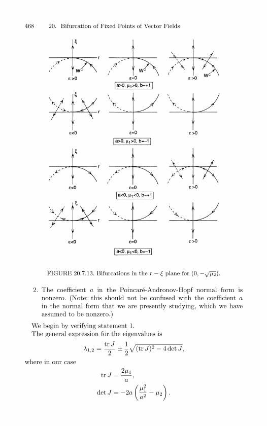
468 20. Bifurcation of Fixed Points of Vector Fields
FIGURE 20.7.13. Bifurcations in the r − ξ plane for (0, −√µ2).
2. The coefficient a in the Poincare-Andronov-Hopf normal form isnonzero. (Note: this should not be confused with the coefficient ain the normal form that we are presently studying, which we haveassumed to be nonzero.)
We begin by verifying statement 1.The general expression for the eigenvalues is
λ1,2 =trJ
2± 1
2
√(trJ)2 − 4 det J,
where in our case
trJ =2µ1
a,
det J = −2a
(µ2
1
a2 − µ2
).
20.7 A Zero and a Pure Imaginary Pair of Eigenvalues 469
We will view µ2 as fixed and µ1 as a parameter; since we are interestedonly in the behavior of the eigenvalues near µ1 = 0, µ2 < 0, we can takethe real part of λ1,2 to be tr J
2 and thus obtain
d
dµ1Re λ =
2a = 0.
Next we check statement 2.We set b = +1 in (20.7.11) and obtain
r = µ1r + arz,
z = µ2 + r2 − z2.
We next put this system into the normal form so that the coefficient ain the Poincare-Andronov-Hopf normal form can be computed. First wetranslate the fixed point to the origin by letting
ρ = r −√
µ21
a− µ2, ξ = z +
µ1
a,
and hence obtain
ρ = µ1
(ρ +
õ2
1
a2 − µ2
)+ a
(ρ +
õ2
1
a2 − µ2
)(ξ − µ1
a
),
ξ = µ2 +
(ρ +
õ2
1
a2 − µ2
)2
−(ξ − µ1
a
)2,
or
ρ = aξ
õ2
1
a2 − µ2 + aρξ,
ξ = 2ρ
õ2
1
a2 − µ2 +2µ1
aξ + ρ2 − ξ2.
We next evaluate this equation on the bifurcation curve µ1 = 0, µ2 < 0and get
ρ = a√|µ2|ξ + aρξ,
ξ = 2√|µ2|ρ + ρ2 − ξ2.
The matrix associated with the linear part of this equation is given by(0 a
√|µ2|
2√|µ2| 0
).
Introducing the linear tranformation(ρξ
)=
(0 −
√|a|2
1 0
)(uv
);
470 20. Bifurcation of Fixed Points of Vector Fields
(uv
)=
1√|a|2
(0
√|a|2
−1 0
)(ρξ
),
the equation becomes(uv
)=
(0 −
√|2aµ2|√
|2aµ2| 0
)(uv
)+
( |a|2 v2 − u2
−|a|uv
).
This is the standard form given in (20.2.13) from which the coefficient a inthe Poincare-Andronov-Hopf normal form can be computed.
From (20.2.14), this coefficient is given by
116
[fuuu + fuvv + guuv + gvvv] +1
16√|2aµ2|
[fuv(fuu + fvv)
− guv(guu + gvv)− fuuguu + fvvgvv],
and all partial derivatives are evaluated at (0, 0).In our case
f ≡ |a|2
v2 − u2,
g ≡ −|a|uv.
Now we work out the partial derivatives (note all third derivatives vanish)
fuu = −2, guu = 0,fuv = 0, guv = −|a|,fvv = |a|, gvv = 0.
Thus, the coefficient a is identically zero. This tells us that we must retain(at least) cubic terms in our normal form in order to get any stabilityinformation concerning the Poincare-Andronov-Hopf bifurcation. (Note: wemight have guessed that this would be the case. Why?) We will completethis analysis in Chapter 33.
Now we must examine Poincare-Andronov-Hopf bifurcations in the re-maining case.
Case III, a > 0. It is straightforward to verify that Poincare-Andronov-Hopf bifurcations occur on µ1 = 0, µ2 > 0 for the branch of fixed pointsgiven by (√
µ2 −µ2
1
a2 ,−µ1
a
)
and that, unfortunately, in this case also, the coefficient in the Poincare-Andronov-Hopf normal form is identically zero.
We now want to summarize these results in the following bifurcationdiagrams.
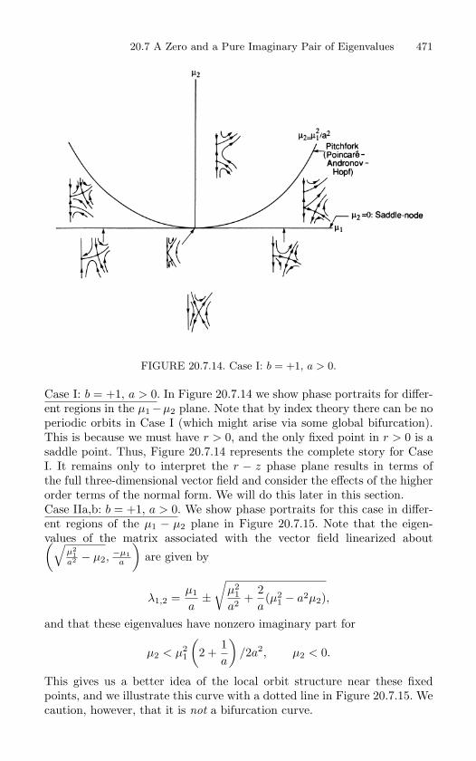
20.7 A Zero and a Pure Imaginary Pair of Eigenvalues 471
FIGURE 20.7.14. Case I: b = +1, a > 0.
Case I: b = +1, a > 0. In Figure 20.7.14 we show phase portraits for differ-ent regions in the µ1−µ2 plane. Note that by index theory there can be noperiodic orbits in Case I (which might arise via some global bifurcation).This is because we must have r > 0, and the only fixed point in r > 0 is asaddle point. Thus, Figure 20.7.14 represents the complete story for CaseI. It remains only to interpret the r − z phase plane results in terms ofthe full three-dimensional vector field and consider the effects of the higherorder terms of the normal form. We will do this later in this section.Case IIa,b: b = +1, a > 0. We show phase portraits for this case in differ-ent regions of the µ1 − µ2 plane in Figure 20.7.15. Note that the eigen-values of the matrix associated with the vector field linearized about(√
µ21
a2 − µ2,−µ1
a
)are given by
λ1,2 =µ1
a±
õ2
1
a2 +2a(µ2
1 − a2µ2),
and that these eigenvalues have nonzero imaginary part for
µ2 < µ21
(2 +
1a
)/2a2, µ2 < 0.
This gives us a better idea of the local orbit structure near these fixedpoints, and we illustrate this curve with a dotted line in Figure 20.7.15. Wecaution, however, that it is not a bifurcation curve.
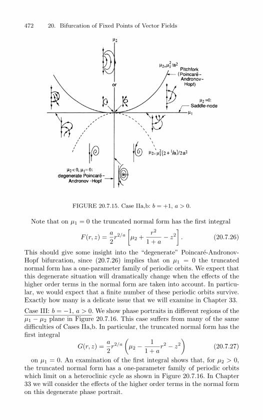
472 20. Bifurcation of Fixed Points of Vector Fields
FIGURE 20.7.15. Case IIa,b: b = +1, a > 0.
Note that on µ1 = 0 the truncated normal form has the first integral
F (r, z) =a
2r2/a
[µ2 +
r2
1 + a− z2
]. (20.7.26)
This should give some insight into the “degenerate” Poincare-Andronov-Hopf bifurcation, since (20.7.26) implies that on µ1 = 0 the truncatednormal form has a one-parameter family of periodic orbits. We expect thatthis degenerate situation will dramatically change when the effects of thehigher order terms in the normal form are taken into account. In particu-lar, we would expect that a finite number of these periodic orbits survive.Exactly how many is a delicate issue that we will examine in Chapter 33.
Case III: b = −1, a > 0. We show phase portraits in different regions of theµ1 − µ2 plane in Figure 20.7.16. This case suffers from many of the samedifficulties of Cases IIa,b. In particular, the truncated normal form has thefirst integral
G(r, z) =a
2r2/a
(µ2 −
11 + a
r2 − z2)
(20.7.27)
on µ1 = 0. An examination of the first integral shows that, for µ2 > 0,the truncated normal form has a one-parameter family of periodic orbitswhich limit on a heteroclinic cycle as shown in Figure 20.7.16. In Chapter33 we will consider the effects of the higher order terms in the normal formon this degenerate phase portrait.
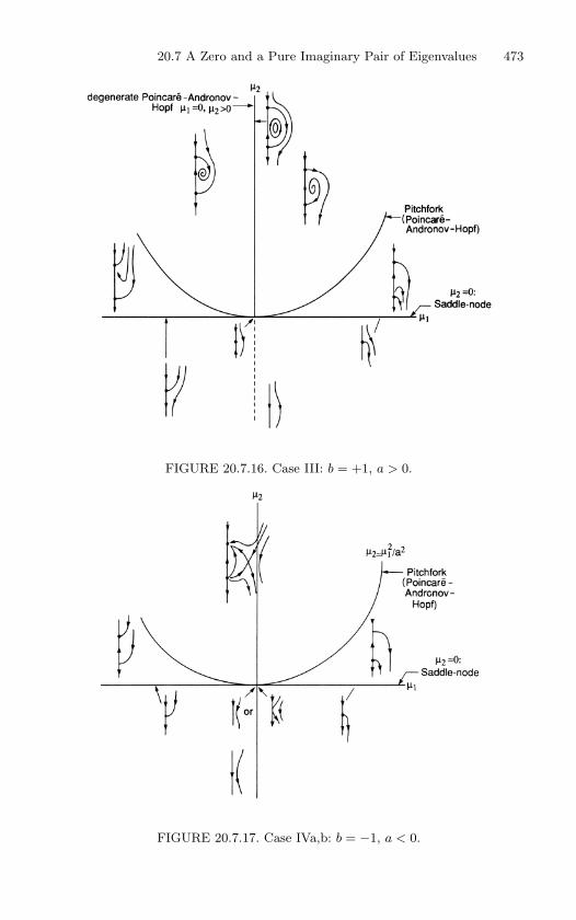
20.7 A Zero and a Pure Imaginary Pair of Eigenvalues 473
FIGURE 20.7.16. Case III: b = +1, a > 0.
FIGURE 20.7.17. Case IVa,b: b = −1, a < 0.
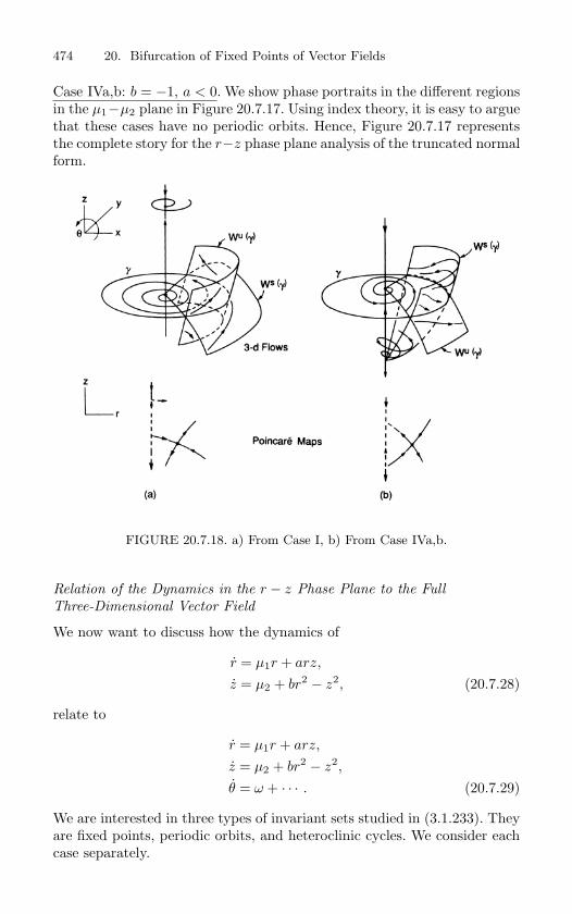
474 20. Bifurcation of Fixed Points of Vector Fields
Case IVa,b: b = −1, a < 0. We show phase portraits in the different regionsin the µ1−µ2 plane in Figure 20.7.17. Using index theory, it is easy to arguethat these cases have no periodic orbits. Hence, Figure 20.7.17 representsthe complete story for the r−z phase plane analysis of the truncated normalform.
FIGURE 20.7.18. a) From Case I, b) From Case IVa,b.
Relation of the Dynamics in the r − z Phase Plane to the Full
Three-Dimensional Vector Field
We now want to discuss how the dynamics of
r = µ1r + arz,
z = µ2 + br2 − z2, (20.7.28)
relate to
r = µ1r + arz,
z = µ2 + br2 − z2,
θ = ω + · · · . (20.7.29)
We are interested in three types of invariant sets studied in (3.1.233). Theyare fixed points, periodic orbits, and heteroclinic cycles. We consider eachcase separately.
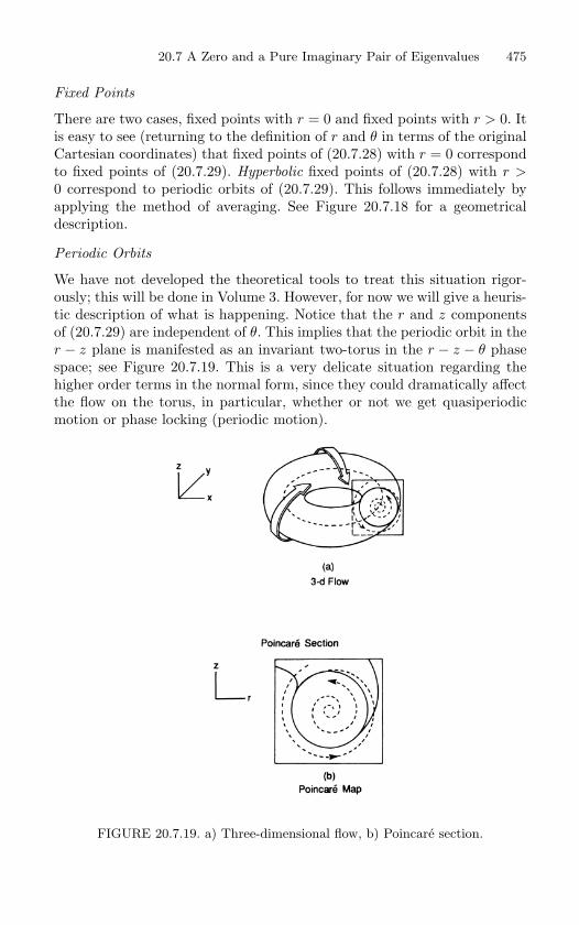
20.7 A Zero and a Pure Imaginary Pair of Eigenvalues 475
Fixed Points
There are two cases, fixed points with r = 0 and fixed points with r > 0. Itis easy to see (returning to the definition of r and θ in terms of the originalCartesian coordinates) that fixed points of (20.7.28) with r = 0 correspondto fixed points of (20.7.29). Hyperbolic fixed points of (20.7.28) with r >0 correspond to periodic orbits of (20.7.29). This follows immediately byapplying the method of averaging. See Figure 20.7.18 for a geometricaldescription.
Periodic Orbits
We have not developed the theoretical tools to treat this situation rigor-ously; this will be done in Volume 3. However, for now we will give a heuris-tic description of what is happening. Notice that the r and z componentsof (20.7.29) are independent of θ. This implies that the periodic orbit in ther − z plane is manifested as an invariant two-torus in the r − z − θ phasespace; see Figure 20.7.19. This is a very delicate situation regarding thehigher order terms in the normal form, since they could dramatically affectthe flow on the torus, in particular, whether or not we get quasiperiodicmotion or phase locking (periodic motion).
FIGURE 20.7.19. a) Three-dimensional flow, b) Poincare section.
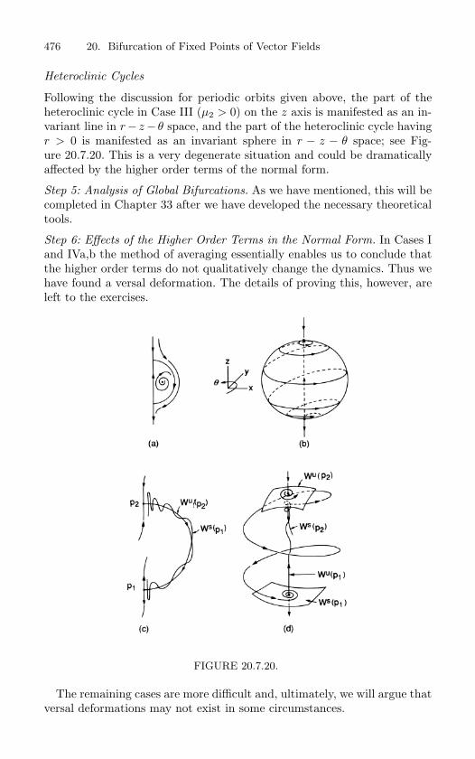
476 20. Bifurcation of Fixed Points of Vector Fields
Heteroclinic Cycles
Following the discussion for periodic orbits given above, the part of theheteroclinic cycle in Case III (µ2 > 0) on the z axis is manifested as an in-variant line in r− z− θ space, and the part of the heteroclinic cycle havingr > 0 is manifested as an invariant sphere in r − z − θ space; see Fig-ure 20.7.20. This is a very degenerate situation and could be dramaticallyaffected by the higher order terms of the normal form.
Step 5: Analysis of Global Bifurcations. As we have mentioned, this will becompleted in Chapter 33 after we have developed the necessary theoreticaltools.
Step 6: Effects of the Higher Order Terms in the Normal Form. In Cases Iand IVa,b the method of averaging essentially enables us to conclude thatthe higher order terms do not qualitatively change the dynamics. Thus wehave found a versal deformation. The details of proving this, however, areleft to the exercises.
FIGURE 20.7.20.
The remaining cases are more difficult and, ultimately, we will argue thatversal deformations may not exist in some circumstances.
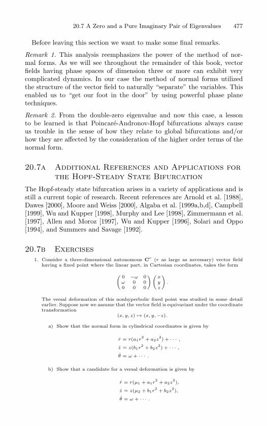
20.7 A Zero and a Pure Imaginary Pair of Eigenvalues 477
Before leaving this section we want to make some final remarks.
Remark 1. This analysis reemphasizes the power of the method of nor-mal forms. As we will see throughout the remainder of this book, vectorfields having phase spaces of dimension three or more can exhibit verycomplicated dynamics. In our case the method of normal forms utilizedthe structure of the vector field to naturally “separate” the variables. Thisenabled us to “get our foot in the door” by using powerful phase planetechniques.
Remark 2. From the double-zero eigenvalue and now this case, a lessonto be learned is that Poincare-Andronov-Hopf bifurcations always causeus trouble in the sense of how they relate to global bifurcations and/orhow they are affected by the consideration of the higher order terms of thenormal form.
20.7a Additional References and Applications forthe Hopf-Steady State Bifurcation
The Hopf-steady state bifurcation arises in a variety of applications and isstill a current topic of research. Recent references are Arnold et al. [1988],Dawes [2000], Moore and Weiss [2000], Algaba et al. [1999a,b,d], Campbell[1999], Wu and Kupper [1998], Murphy and Lee [1998], Zimmermann et al.[1997], Allen and Moroz [1997], Wu and Kupper [1996], Solari and Oppo[1994], and Summers and Savage [1992].
20.7b Exercises1. Consider a three-dimensional autonomous Cr (r as large as necessary) vector field
having a fixed point where the linear part, in Cartesian coordinates, takes the form
( 0 −ω 0ω 0 00 0 0
)(xyz
).
The versal deformation of this nonhyperbolic fixed point was studied in some detailearlier. Suppose now we assume that the vector field is equivariant under the coordinatetransformation
(x, y, z) → (x, y, −z).
a) Show that the normal form in cylindrical coordinates is given by
r = r(a1r2 + a2z
2) + · · · ,
z = z(b1r2 + b2z
2) + · · · ,
θ = ω + · · · .
b) Show that a candidate for a versal deformation is given by
r = r(µ1 + a1r2 + a2z
2),
z = z(µ2 + b1r2 + b2z
2),
θ = ω + · · · .
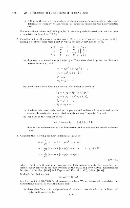
478 20. Bifurcation of Fixed Points of Vector Fields
c) Following the steps in the analysis of the nonsymmetric case, analyze this versaldeformation completely, addressing all issues discussed for the nonsymmetriccase.
For an excellent review and bibliography of this nonhyperbolic fixed point with varioussymmetries see Langford [1985].
2. Consider a four-dimensional autonomous Cr (r as large as necessary) vector fieldhaving a nonhyperbolic fixed point at which the linear part has the form
0 −ω1 0 0ω1 0 0 00 0 0 −ω20 0 ω2 0
wxyz
.
a) Suppose mω1 + nω2 = 0, |m| + |n| ≤ 4. Then show that in polar coordinates anormal form is given by
r1 = a1r31 + a2r1r
22 + · · · ,
r2 = b1r21r2 + b2r
31 + · · · ,
θ1 = ω1 + · · · ,
θ2 = ω2 + · · · .
b) Show that a candidate for a versal deformation is given by
r1 = µ1r1 + a1r31 + a2r1r
22 ,
r2 = µ2r2 + b1r21r2 + b2r
31 ,
θ1 = ω1 + · · · ,
θ2 = ω2 + · · · .
c) Analyze this versal deformation completely and address all issues raised in thissection. In particular, under what conditions may “three-tori” arise?
d) For each of the resonant cases
mω1 + nω2 = 0, |m| + |n| ≤ 4,
discuss the codimension of the bifurcation and candidates for versal deforma-tions.
3. Consider the following ordinary differential equation
x =ω
√3(y − z) + [ε − µ(x2 − yz)]x,
y =ω
√3(z − x) + [ε − µ(y2 − xz)]y, (x, y, z) ∈ R
3
z =ω
√3(x − y) + [ε − µ(z2 − xy)]z,
(20.7.30)
where ε > 0, µ > 0, and ω are parameters. This system is useful for modeling andsimulating synchronous machine systems in the study of power system dynamics; seeKaplan and Yardeni [1989] and Kaplan and Kottick [1983], [1985], [1987].
It should be obvious that(x, y, z) = (0, 0, 0)
is a fixed point of (20.7.30) for all parameter values. We are interested in studying thebifurcations associated with this fixed point.
a) Show that for ε = 0 the eigenvalues of the matrix associated with the linearizedvector field are given by
0, ±iω.
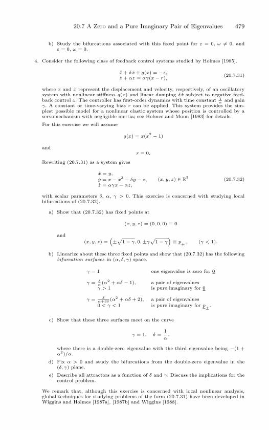
20.7 A Zero and a Pure Imaginary Pair of Eigenvalues 479
b) Study the bifurcations associated with this fixed point for ε = 0, ω = 0, andε = 0, ω = 0.
4. Consider the following class of feedback control systems studied by Holmes [1985].
x + δx + g(x) = −z,z + αz = αγ(x − r), (20.7.31)
where x and x represent the displacement and velocity, respectively, of an oscillatorysystem with nonlinear stiffness g(x) and linear damping δx subject to negative feed-back control z. The controller has first-order dynamics with time constant 1
α and gainγ. A constant or time-varying bias r can be applied. This system provides the sim-plest possible model for a nonlinear elastic system whose position is controlled by aservomechanism with negligible inertia; see Holmes and Moon [1983] for details.
For this exercise we will assume
g(x) = x(x2 − 1)
andr = 0.
Rewriting (20.7.31) as a system gives
x = y,
y = x − x3 − δy − z,
z = αγx − αz,(x, y, z) ∈ R
3 (20.7.32)
with scalar parameters δ, α, γ > 0. This exercise is concerned with studying localbifurcations of (20.7.32).
a) Show that (20.7.32) has fixed points at
(x, y, z) = (0, 0, 0) ≡ 0
and(x, y, z) =
(±√
1 − γ, 0, ±γ√
1 − γ)
≡ p±, (γ < 1).
b) Linearize about these three fixed points and show that (20.7.32) has the followingbifurcation surfaces in (α, δ, γ) space.
γ = 1 one eigenvalue is zero for 0
γ = δα (α2 + αδ − 1), a pair of eigenvaluesγ > 1 is pure imaginary for 0
γ = δα+3δ (α2 + αδ + 2), a pair of eigenvalues0 < γ < 1 is pure imaginary for p±.
c) Show that these three surfaces meet on the curve
γ = 1, δ =1α
,
where there is a double-zero eigenvalue with the third eigenvalue being −(1 +α2)/α.
d) Fix α > 0 and study the bifurcations from the double-zero eigenvalue in the(δ, γ) plane.
e) Describe all attractors as a function of δ and γ. Discuss the implications for thecontrol problem.
We remark that, although this exercise is concerned with local nonlinear analysis,global techniques for studying problems of the form (20.7.31) have been developed inWiggins and Holmes [1987a], [1987b] and Wiggins [1988].
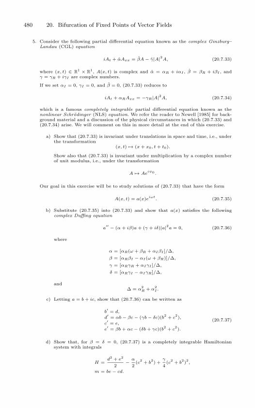
480 20. Bifurcation of Fixed Points of Vector Fields
5. Consider the following partial differential equation known as the complex Ginzburg–Landau (CGL) equation
iAt + αAxx = βA − γ|A|2A, (20.7.33)
where (x, t) ∈ R1 × R
1, A(x, t) is complex and α = αR + iαI , β = βR + iβI , andγ = γR + iγI are complex numbers.
If we set αI = 0, γI = 0, and β = 0, (20.7.33) reduces to
iAt + αRAxx = −γR|A|2A, (20.7.34)
which is a famous completely integrable partial differential equation known as thenonlinear Schrodinger (NLS) equation. We refer the reader to Newell [1985] for back-ground material and a discussion of the physical circumstances in which (20.7.33) and(20.7.34) arise. We will comment on this in more detail at the end of this exercise.
a) Show that (20.7.33) is invariant under translations in space and time, i.e., underthe transformation
(x, t) → (x + x0, t + t0).
Show also that (20.7.33) is invariant under multiplication by a complex numberof unit modulus, i.e., under the transformation
A → Aeiψ0 .
Our goal in this exercise will be to study solutions of (20.7.33) that have the form
A(x, t) = a(x)eiωt. (20.7.35)
b) Substitute (20.7.35) into (20.7.33) and show that a(x) satisfies the followingcomplex Duffing equation
a′′ − (α + iβ)a + (γ + iδ)|a|2a = 0, (20.7.36)
where
α = [αR(ω + βR + αIβI ]/∆,
β = [αRβI − αI(ω + βR)]/∆,
γ = [αRγR + αIγI ]/∆,
δ = [αRγI − αIγR]/∆,
and∆ = α
2R + α
2I .
c) Letting a = b + ic, show that (20.7.36) can be written as
b′ = d,
d′ = αb − βc − (γb − δc)(b2 + c
2),c
′ = e,
e′ = βb + αc − (δb + γc)(b2 + c
2).
(20.7.37)
d) Show that, for β = δ = 0, (20.7.37) is a completely integrable Hamiltoniansystem with integrals
H =d2 + e2
2− α
2(c2 + b
2) +γ
4(c2 + b
2)2,
m = be − cd.
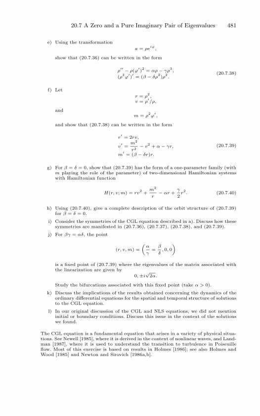
20.7 A Zero and a Pure Imaginary Pair of Eigenvalues 481
e) Using the transformationa = ρe
iϕ,
show that (20.7.36) can be written in the form
ρ′′ − ρ(ϕ′)2 = αρ − γρ
3,
(ρ2ϕ
′)′ = (β − δρ2)ρ2
.(20.7.38)
f) Letr = ρ
2,
v = ρ′/ρ,
andm = ρ
2ϕ
′,
and show that (20.7.38) can be written in the form
r′ = 2rv,
v′ =
m2
r2− v
2 + α − γr,
m′ = (β − δr)r.
(20.7.39)
g) For β = δ = 0, show that (20.7.39) has the form of a one-parameter family (withm playing the role of the parameter) of two-dimensional Hamiltonian systemswith Hamiltonian function
H(r, v; m) = rv2 +
m2
r− αr +
γ
2r2. (20.7.40)
h) Using (20.7.40), give a complete description of the orbit structure of (20.7.39)for β = δ = 0.
i) Consider the symmetries of the CGL equation described in a). Discuss how thesesymmetries are manifested in (20.7.36), (20.7.37), (20.7.38), and (20.7.39).
j) For βγ = αδ, the point
(r, v, m) =(
α
γ=
β
δ, 0, 0
)
is a fixed point of (20.7.39) where the eigenvalues of the matrix associated withthe linearization are given by
0, ±i√
2α.
Study the bifurcations associated with this fixed point (take α > 0).
k) Discuss the implications of the results obtained concerning the dynamics of theordinary differential equations for the spatial and temporal structure of solutionsto the CGL equation.
l) In our original discussion of the CGL and NLS equations, we did not mentioninitial or boundary conditions. Discuss this issue in the context of the solutionswe found.
The CGL equation is a fundamental equation that arises in a variety of physical situa-tions. See Newell [1985], where it is derived in the context of nonlinear waves, and Land-man [1987], where it is used to understand the transition to turbulence in Poiseuilleflow. Most of this exercise is based on results in Holmes [1986]; see also Holmes andWood [1985] and Newton and Sirovich [1986a,b].
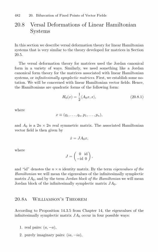
482 20. Bifurcation of Fixed Points of Vector Fields
20.8 Versal Deformations of Linear HamiltonianSystems
In this section we describe versal deformation theory for linear Hamiltoniansystems that is very similar to the theory developed for matrices in Section20.5.
The versal deformation theory for matrices used the Jordan canonicalform in a variety of ways. Similarly, we need something like a Jordancanonical form theory for the matrices associated with linear Hamiltoniansystems, or infinitesimally symplectic matrices. First, we establish some no-tation. We will be concerned with linear Hamiltonian vector fields. Hence,the Hamiltonians are quadratic forms of the following form:
H0(x) =12〈A0x, x〉, (20.8.1)
wherex ≡ (q1, . . . , qn, p1, . . . , pn),
and A0 is a 2n × 2n real symmetric matrix. The associated Hamiltonianvector field is then given by
x = JA0x,
where
J =(
0 id−id 0
),
and “id” denotes the n×n identity matrix. By the term eigenvalues of the
Hamiltonian we will mean the eigenvalues of the infinitesimally symplecticmatrix JA0, and by the term Jordan block of the Hamiltonian we will meanJordan block of the infinitesimally symplectic matrix JA0.
20.8a Williamson’s Theorem
According to Proposition 14.3.5 from Chapter 14, the eigenvalues of theinfinitesimally symplectic matrix JA0 occur in four possible ways:
1. real pairs: (a,−a),
2. purely imaginary pairs: (ia,−ia),
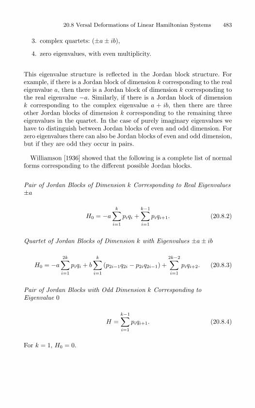
20.8 Versal Deformations of Linear Hamiltonian Systems 483
3. complex quartets: (±a± ib),
4. zero eigenvalues, with even multiplicity.
This eigenvalue structure is reflected in the Jordan block structure. Forexample, if there is a Jordan block of dimension k corresponding to the realeigenvalue a, then there is a Jordan block of dimension k corresponding tothe real eigenvalue −a. Similarly, if there is a Jordan block of dimensionk corresponding to the complex eigenvalue a + ib, then there are threeother Jordan blocks of dimension k corresponding to the remaining threeeigenvalues in the quartet. In the case of purely imaginary eigenvalues wehave to distinguish between Jordan blocks of even and odd dimension. Forzero eigenvalues there can also be Jordan blocks of even and odd dimension,but if they are odd they occur in pairs.
Williamson [1936] showed that the following is a complete list of normalforms corresponding to the different possible Jordan blocks.
Pair of Jordan Blocks of Dimension k Corresponding to Real Eigenvalues
±a
H0 = −ak∑
i=1
piqi +k−1∑i=1
piqi+1. (20.8.2)
Quartet of Jordan Blocks of Dimension k with Eigenvalues ±a± ib
H0 = −a
2k∑i=1
piqi + b
k∑i=1
(p2i−1q2i − p2iq2i−1) +2k−2∑i=1
piqi+2. (20.8.3)
Pair of Jordan Blocks with Odd Dimension k Corresponding to
Eigenvalue 0
H =k−1∑i=1
piqi+1. (20.8.4)
For k = 1, H0 = 0.
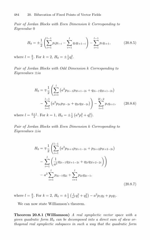
484 20. Bifurcation of Fixed Points of Vector Fields
Pair of Jordan Blocks with Even Dimension k Corresponding to
Eigenvalue 0
H0 = ±12
(l−1∑i=1
pipl−i −l∑
i=1
qiql+1−i
)−
l−1∑i=1
piqi+1, (20.8.5)
where l = k2 . For k = 2, H0 = ±1
2q21 .
Pair of Jordan Blocks with Odd Dimension k Corresponding to
Eigenvalues ±ia
H0 = ∓12
(l∑
i=1
(a2p2i−1p2l+1−2i + q2i−1q2l+1−2i
)
−l−1∑i=1
(a2p2ip2l−2i + q2iq2l−2i
))−
2l−2∑i=1
piqi+1, (20.8.6)
where l = k+12 . For k = 1, H0 = ±1
2
(a2p2
1 + q21).
Pair of Jordan Blocks with Even Dimension k Corresponding to
Eigenvalues ±ia
H0 = ∓12
(l−1∑i=1
(a2p2i+1p2l+1−2i + p2i+2p2l+2−2i
)
−l∑
i=1
(1a2 q2i−1q2l+1−2i + q2iq2l+2−2i
))
− a2l∑
i=1
p2i−1q2i +l∑
i=1
p2iq2i−1,
(20.8.7)
where l = k2 . For k = 2, H0 = ±1
2
( 1a2 q2
1 + q22)− a2p1q2 + p2q1.
We can now state Williamson’s theorem.
Theorem 20.8.1 (Williamson) A real symplectic vector space with a
given quadratic form H0 can be decomposed into a direct sum of skew or-
thogonal real symplectic subspaces in such a way that the quadratic form
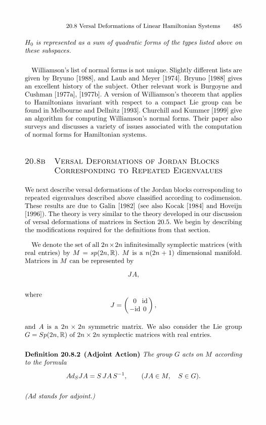
20.8 Versal Deformations of Linear Hamiltonian Systems 485
H0 is represented as a sum of quadratic forms of the types listed above on
these subspaces.
Williamson’s list of normal forms is not unique. Slightly different lists aregiven by Bryuno [1988], and Laub and Meyer [1974]. Bryuno [1988] givesan excellent history of the subject. Other relevant work is Burgoyne andCushman [1977a], [1977b]. A version of Williamson’s theorem that appliesto Hamiltonians invariant with respect to a compact Lie group can befound in Melbourne and Dellnitz [1993]. Churchill and Kummer [1999] givean algorithm for computing Williamson’s normal forms. Their paper alsosurveys and discusses a variety of issues associated with the computationof normal forms for Hamiltonian systems.
20.8b Versal Deformations of Jordan BlocksCorresponding to Repeated Eigenvalues
We next describe versal deformations of the Jordan blocks corresponding torepeated eigenvalues described above classified according to codimension.These results are due to Galin [1982] (see also Kocak [1984] and Hoveijn[1996]). The theory is very similar to the theory developed in our discussionof versal deformations of matrices in Section 20.5. We begin by describingthe modifications required for the definitions from that section.
We denote the set of all 2n×2n infinitesimally symplectic matrices (withreal entries) by M = sp(2n, R). M is a n(2n + 1) dimensional manifold.Matrices in M can be represented by
JA,
where
J =(
0 id−id 0
),
and A is a 2n × 2n symmetric matrix. We also consider the Lie groupG = Sp(2n, R) of 2n× 2n symplectic matrices with real entries.
Definition 20.8.2 (Adjoint Action) The group G acts on M according
to the formula
AdSJA = S JA S−1, (JA ∈ M, S ∈ G).
(Ad stands for adjoint.)
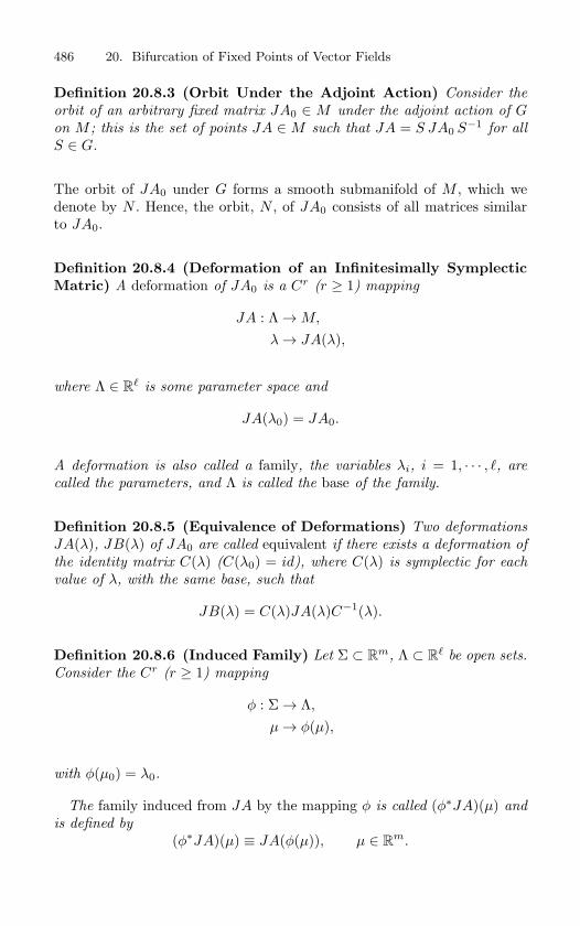
486 20. Bifurcation of Fixed Points of Vector Fields
Definition 20.8.3 (Orbit Under the Adjoint Action) Consider the
orbit of an arbitrary fixed matrix JA0 ∈ M under the adjoint action of Gon M ; this is the set of points JA ∈ M such that JA = S JA0 S−1 for all
S ∈ G.
The orbit of JA0 under G forms a smooth submanifold of M , which wedenote by N . Hence, the orbit, N , of JA0 consists of all matrices similarto JA0.
Definition 20.8.4 (Deformation of an Infinitesimally SymplecticMatric) A deformation of JA0 is a Cr (r ≥ 1) mapping
JA : Λ→M,
λ→ JA(λ),
where Λ ∈ R is some parameter space and
JA(λ0) = JA0.
A deformation is also called a family, the variables λi, i = 1, · · · , , are
called the parameters, and Λ is called the base of the family.
Definition 20.8.5 (Equivalence of Deformations) Two deformations
JA(λ), JB(λ) of JA0 are called equivalent if there exists a deformation of
the identity matrix C(λ) (C(λ0) = id), where C(λ) is symplectic for each
value of λ, with the same base, such that
JB(λ) = C(λ)JA(λ)C−1(λ).
Definition 20.8.6 (Induced Family) Let Σ ⊂ Rm, Λ ⊂ R
be open sets.
Consider the Cr (r ≥ 1) mapping
φ : Σ→ Λ,
µ→ φ(µ),
with φ(µ0) = λ0.
The family induced from JA by the mapping φ is called (φ∗JA)(µ) and
is defined by
(φ∗JA)(µ) ≡ JA(φ(µ)), µ ∈ Rm.
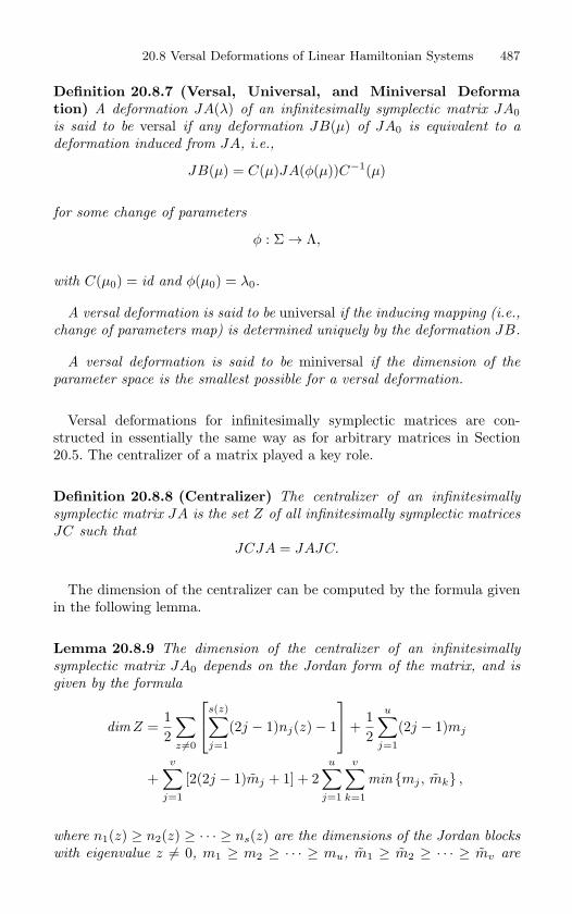
20.8 Versal Deformations of Linear Hamiltonian Systems 487
Definition 20.8.7 (Versal, Universal, and Miniversal Deformation) A deformation JA(λ) of an infinitesimally symplectic matrix JA0is said to be versal if any deformation JB(µ) of JA0 is equivalent to a
deformation induced from JA, i.e.,
JB(µ) = C(µ)JA(φ(µ))C−1(µ)
for some change of parameters
φ : Σ → Λ,
with C(µ0) = id and φ(µ0) = λ0.
A versal deformation is said to be universal if the inducing mapping (i.e.,
change of parameters map) is determined uniquely by the deformation JB.
A versal deformation is said to be miniversal if the dimension of the
parameter space is the smallest possible for a versal deformation.
Versal deformations for infinitesimally symplectic matrices are con-structed in essentially the same way as for arbitrary matrices in Section20.5. The centralizer of a matrix played a key role.
Definition 20.8.8 (Centralizer) The centralizer of an infinitesimally
symplectic matrix JA is the set Z of all infinitesimally symplectic matrices
JC such that
JCJA = JAJC.
The dimension of the centralizer can be computed by the formula givenin the following lemma.
Lemma 20.8.9 The dimension of the centralizer of an infinitesimally
symplectic matrix JA0 depends on the Jordan form of the matrix, and is
given by the formula
dimZ =12
∑z =0
s(z)∑
j=1
(2j − 1)nj(z)− 1
+
12
u∑j=1
(2j − 1)mj
+v∑
j=1
[2(2j − 1)mj + 1] + 2u∑
j=1
v∑k=1
min mj , mk ,
where n1(z) ≥ n2(z) ≥ · · · ≥ ns(z) are the dimensions of the Jordan blocks
with eigenvalue z = 0, m1 ≥ m2 ≥ · · · ≥ mu, m1 ≥ m2 ≥ · · · ≥ mv are
488 20. Bifurcation of Fixed Points of Vector Fields
the dimensions of the Jordan blocks with eigenvalue z = 0, the numbers
mj being even, while mj are odd (only one block out of each pair of Jordan
blocks of odd dimension is taken into account).
The relationship between the dimension of the centralizer and the orbitof an infinitesimally symplectic matrix under the adjoint action of G isgiven in the following proposition.
Proposition 20.8.10 The dimension of the centralizer of an arbitrary in-
finitesimally symplectic matrix JA0 is equal to the codimension of its orbit
in the space M of infinitesimally symplectic matrices.
The following proposition is analogous to Proposition 20.5.8, and provenin the same way.
Proposition 20.8.11 A deformation JA(λ) of an arbitrary infinitesi-
mally symplectic matrix JA0 is versal if and only if the mapping JA(λ)is transversal to N at the point λ = λ0.
Versal deformations for infinitesimally symplectic matrices are computedin exactly the same way as for arbitrary matrices as described in Section20.5. For a Jordan block JA0, a versal deformation is of the form
JA0 + JB,
where B is symmetric, and has entries consisting of the appropriate numberof parameters (as given by Lemma 20.8.9), with the parameters occurringin such a way that JB is not in the tangent space of N . Lemma 20.5.11and the inner product on the space of matrices (equation (20.5.11)) canbe used to verify that JB has this property. Once this has been done, wecan also recover A0 +B (by multiplying by J−1, and write a correspondingversal deformation of the Hamiltonian, or quadratic form (20.8.1). Galin[1982] has made a list of these quadratic forms for codimension ≤ 2, whichwe now reproduce.
20.8c Versal Deformations of QuadraticHamiltonians of Codimension ≤ 2
First, we introduce some notation. For a given eigenvalue λ, we will de-note the corresponding Jordan block of dimension (or order) k by (λ)k.
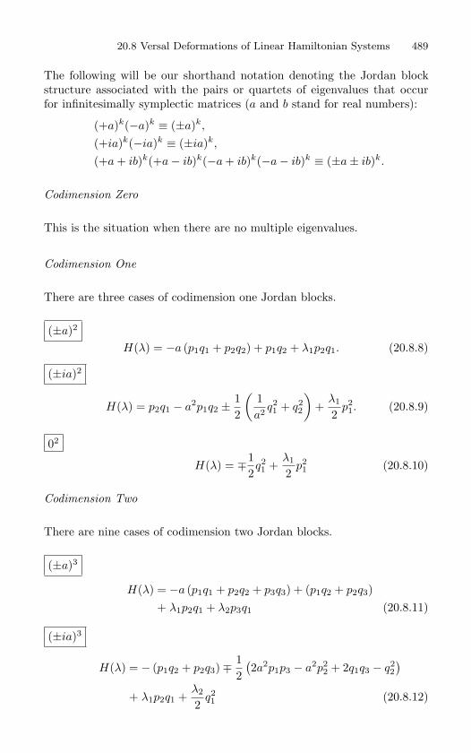
20.8 Versal Deformations of Linear Hamiltonian Systems 489
The following will be our shorthand notation denoting the Jordan blockstructure associated with the pairs or quartets of eigenvalues that occurfor infinitesimally symplectic matrices (a and b stand for real numbers):
(+a)k(−a)k ≡ (±a)k,
(+ia)k(−ia)k ≡ (±ia)k,
(+a + ib)k(+a− ib)k(−a + ib)k(−a− ib)k ≡ (±a± ib)k.
Codimension Zero
This is the situation when there are no multiple eigenvalues.
Codimension One
There are three cases of codimension one Jordan blocks.
(±a)2
H(λ) = −a (p1q1 + p2q2) + p1q2 + λ1p2q1. (20.8.8)
(±ia)2
H(λ) = p2q1 − a2p1q2 ±12
(1a2 q2
1 + q22
)+
λ1
2p21. (20.8.9)
02
H(λ) = ∓12q21 +
λ1
2p21 (20.8.10)
Codimension Two
There are nine cases of codimension two Jordan blocks.
(±a)3
H(λ) = −a (p1q1 + p2q2 + p3q3) + (p1q2 + p2q3)+ λ1p2q1 + λ2p3q1 (20.8.11)
(±ia)3
H(λ) = − (p1q2 + p2q3)∓12(2a2p1p3 − a2p2
2 + 2q1q3 − q22)
+ λ1p2q1 +λ2
2q21 (20.8.12)
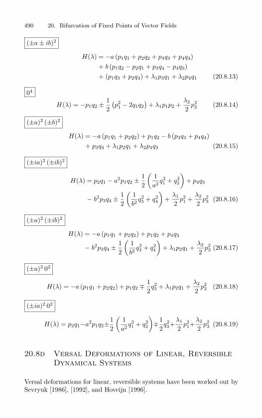
490 20. Bifurcation of Fixed Points of Vector Fields
(±a± ib)2
H(λ) = −a (p1q1 + p2q2 + p3q3 + p4q4)+ b (p1q2 − p2q1 + p3q4 − p4q3)+ (p1q3 + p2q4) + λ1p3q1 + λ2p4q1 (20.8.13)
04
H(λ) = −p1q2 ±12(p21 − 2q1q2
)+ λ1p1p2 +
λ2
2p22 (20.8.14)
(±a)2 (±b)2
H(λ) = −a (p1q1 + p2q2) + p1q2 − b (p3q3 + p4q4)+ p3q4 + λ1p2q1 + λ2p4q3 (20.8.15)
(±ia)2 (±ib)2
H(λ) = p2q1 − a2p1q2 ±12
(1a2 q2
1 + q22
)+ p4q3
− b2p3q4 ±12
(1b2 q2
3 + q24
)+
λ1
2p21 +
λ2
2p23 (20.8.16)
(±a)2 (±ib)2
H(λ) = −a (p1q1 + p2q2) + p1q2 + p4q3
− b2p3q4 ±12
(1b2 q2
3 + q24
)+ λ1p2q1 +
λ2
2p23 (20.8.17)
(±a)2 02
H(λ) = −a (p1q1 + p2q2) + p1q2 ∓12q23 + λ1p2q1 +
λ2
2p23 (20.8.18)
(±ia)2 02
H(λ) = p2q1−a2p1q2±12
(1a2 q2
1 + q22
)∓1
2q23+
λ1
2p21+
λ2
2p23 (20.8.19)
20.8d Versal Deformations of Linear, ReversibleDynamical Systems
Versal deformations for linear, reversible systems have been worked out bySevryuk [1986], [1992], and Hoveijn [1996].
20.9 Elementary Hamiltonian Bifurcations 491
20.8e Exercises1. Compute the form of the quadratic Hamiltonians in the codimension zero cases. Also
compute the associated infinitesimally symplectic matrices.
2. For the codimension one versal deformations, compute the associated infinitesimallysymplectic matrices.
3. Prove that the three codimension one cases in Galin’s list are indeed versal deforma-tions.
4. Eigenvalue Movement. For the codimension one versal deformations, sketch the po-sitions of the eigenvalues in the complex plane for λ1 < 0, λ1 = 0, and λ1 > 0. Indicatehow the eigenvalues move as λ1 is varied from positive to negative. The case (±ia)2
is known as the Hamiltonian Hopf bifurcation. However, as pointed out in Meyer andHall [1992], Hopf had nothing to do with the study of the bifurcations associated withthis case. van der Meer [1985] and Meyer and Hall [1992] give discussions that put thisin the correct historical context. An elementary exposition of the Hamiltonian Hopfbifurcation is given by Lahiri and Roy [2001].
5. Compute the normal form (the leading order terms beyond quadratic) for the Hamil-tonian Hopf bifurcation.
6. Compute the normal form (the leading order terms beyond quadratic) for the the case(±a)2.
20.9 Elementary Hamiltonian Bifurcations
In this section we describe some of the basic elementary Hamiltonian bifur-cations. Hamiltonian bifurcation theory is a rapidly developing area. Thearticles of Meyer [1975], [1986], and Golubitsky et al. [1995] and the booksof Arnold et al. [1988] and Meyer and Hall [1992] provide a good overview ofthe subject of Hamiltonian bifurcations of equilibrium points and periodicorbits, with and without symmetry.
20.9a One Degree-of-Freedom Systems
We now describe three elementary bifurcations of equilibrium points inone-degree-of-freedom Hamiltonian systems in the spirit of the saddle-node, pitchfork, and Hopf bifurcations for general vector fields that wedescribed earlier. The following discussion is taken from Golubitsky andStewart [1987].
Hamiltonian Saddle Node
The analog of the saddle-node bifurcation for Hamiltonian systems is a sit-uation where as a parameter is varied two equilibria, a saddle and a center,
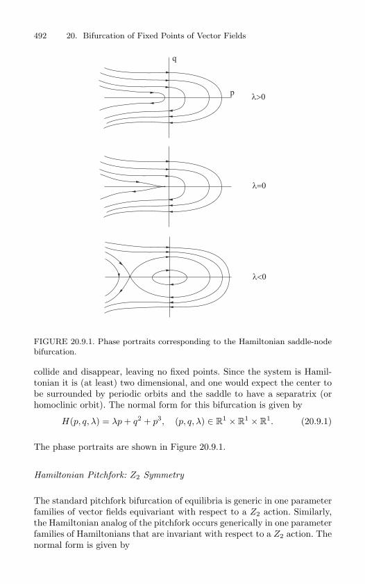
492 20. Bifurcation of Fixed Points of Vector Fields
λ>0
λ<0
λ=0
p
q
FIGURE 20.9.1. Phase portraits corresponding to the Hamiltonian saddle-node
bifurcation.
collide and disappear, leaving no fixed points. Since the system is Hamil-tonian it is (at least) two dimensional, and one would expect the center tobe surrounded by periodic orbits and the saddle to have a separatrix (orhomoclinic orbit). The normal form for this bifurcation is given by
H(p, q, λ) = λp + q2 + p3, (p, q, λ) ∈ R1 × R
1 × R1. (20.9.1)
The phase portraits are shown in Figure 20.9.1.
Hamiltonian Pitchfork: Z2 Symmetry
The standard pitchfork bifurcation of equilibria is generic in one parameterfamilies of vector fields equivariant with respect to a Z2 action. Similarly,the Hamiltonian analog of the pitchfork occurs generically in one parameterfamilies of Hamiltonians that are invariant with respect to a Z2 action. Thenormal form is given by
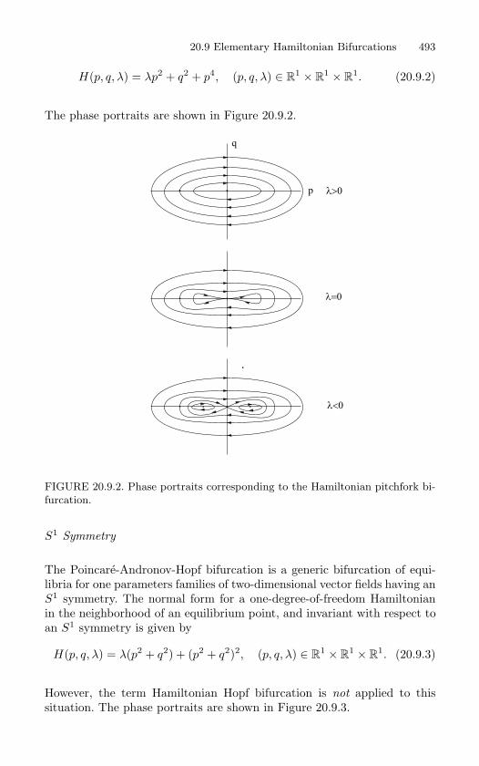
20.9 Elementary Hamiltonian Bifurcations 493
H(p, q, λ) = λp2 + q2 + p4, (p, q, λ) ∈ R1 × R
1 × R1. (20.9.2)
The phase portraits are shown in Figure 20.9.2.
p
q
FIGURE 20.9.2. Phase portraits corresponding to the Hamiltonian pitchfork bi-
furcation.
S1 Symmetry
The Poincare-Andronov-Hopf bifurcation is a generic bifurcation of equi-libria for one parameters families of two-dimensional vector fields having anS1 symmetry. The normal form for a one-degree-of-freedom Hamiltonianin the neighborhood of an equilibrium point, and invariant with respect toan S1 symmetry is given by
H(p, q, λ) = λ(p2 + q2) + (p2 + q2)2, (p, q, λ) ∈ R1 × R
1 × R1. (20.9.3)
However, the term Hamiltonian Hopf bifurcation is not applied to thissituation. The phase portraits are shown in Figure 20.9.3.
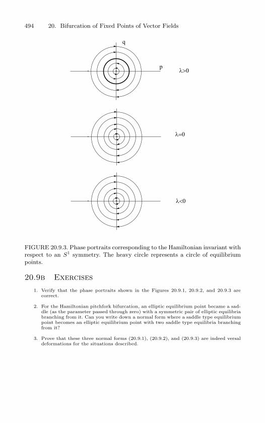
494 20. Bifurcation of Fixed Points of Vector Fields
p
q
FIGURE 20.9.3. Phase portraits corresponding to the Hamiltonian invariant with
respect to an S1 symmetry. The heavy circle represents a circle of equilibrium
points.
20.9b Exercises1. Verify that the phase portraits shown in the Figures 20.9.1, 20.9.2, and 20.9.3 are
correct.
2. For the Hamiltonian pitchfork bifurcation, an elliptic equilibrium point became a sad-dle (as the parameter passed through zero) with a symmetric pair of elliptic equilibriabranching from it. Can you write down a normal form where a saddle type equilibriumpoint becomes an elliptic equilibrium point with two saddle type equilibria branchingfrom it?
3. Prove that these three normal forms (20.9.1), (20.9.2), and (20.9.3) are indeed versaldeformations for the situations described.
20.9 Elementary Hamiltonian Bifurcations 495
20.9c Bifurcations Near Resonant EllipticEquilibrium Points
Bifurcations near resonant elliptic equilibrium points have been studiedin detail by a number of authors. Arnold et al. [1988] and Meyer and Hall[1992] give excellent surveys. A great deal is known about bifurcations nearresonant elliptic equilibria in the two degree-of-freedom case. There aretwo natural bifurcation parameters. One is the energy and the other is the“detuning”, which allows one to study the passage through the resonance.The main reason so much is known in the two degree-of-freedom case isthat the truncated normal form is integrable. Very little is known aboutbifurcations in resonant elliptic equilibria in n degree- of-freedom systems,n ≥ 3, when the multiplicity of the resonance is larger than two (thetruncated normal forms associated with multiplicity one resonances arestill integrable, regardless of the number of degrees of freedom, provided itis finite). Hoveijn [1992] and Haller and Wiggins [1996] give recent surveysof the literature related to resonant elliptic equilibria with three or moredegrees-of-freedom.
We now describe how one analyzes bifurcations near resonant equilibriain two degree-of-freedom Hamiltonian systems.
First we recall some basic results from Section 19.10b. The quadraticpart of the Hamiltonian is given by
H(z1, z1, z2, z2) =ω1
2|z1|2 +
ω2
2|z2|2,
and is said to be in resonance provided ω1ω2
is a rational number. The trun-cated normal forms for the 1 : 1 (semisimple), 1 : 2, and 1 : 3 resonanceswere computed and found to be:
1:1 Resonance
H(z1, z1, z2, z2) =12(1 + δ1)|z1|2 +
12(1 + δ2)|z2|2
+ c1111|z1|2|z2|2 + c0022|z2|4 + c2200|z1|4
+ 2|c2011|Rez21 z1z2 + 2|c1102|Rez1z2z
22 + 2|c2002|Rez2
1 z22 ,
1:2 Resonance
H(z1, z1, z2, z2) =12(1 + δ1)|z1|2 + (1 + δ2)|z2|2 + 2|c2001|Rez2
1 z2,
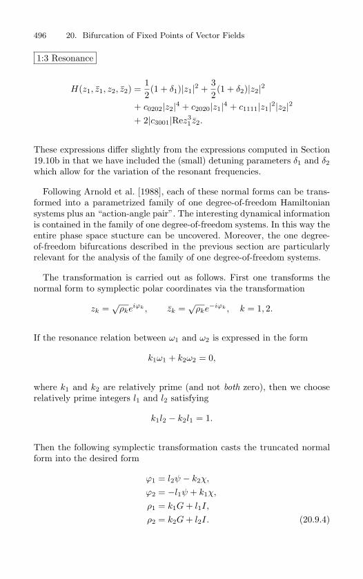
496 20. Bifurcation of Fixed Points of Vector Fields
1:3 Resonance
H(z1, z1, z2, z2) =12(1 + δ1)|z1|2 +
32(1 + δ2)|z2|2
+ c0202|z2|4 + c2020|z1|4 + c1111|z1|2|z2|2
+ 2|c3001|Rez31 z2.
These expressions differ slightly from the expressions computed in Section19.10b in that we have included the (small) detuning parameters δ1 and δ2which allow for the variation of the resonant frequencies.
Following Arnold et al. [1988], each of these normal forms can be trans-formed into a parametrized family of one degree-of-freedom Hamiltoniansystems plus an “action-angle pair”. The interesting dynamical informationis contained in the family of one degree-of-freedom systems. In this way theentire phase space stucture can be uncovered. Moreover, the one degree-of-freedom bifurcations described in the previous section are particularlyrelevant for the analysis of the family of one degree-of-freedom systems.
The transformation is carried out as follows. First one transforms thenormal form to symplectic polar coordinates via the transformation
zk =√
ρkeiϕk , zk =√
ρke−iϕk , k = 1, 2.
If the resonance relation between ω1 and ω2 is expressed in the form
k1ω1 + k2ω2 = 0,
where k1 and k2 are relatively prime (and not both zero), then we chooserelatively prime integers l1 and l2 satisfying
k1l2 − k2l1 = 1.
Then the following symplectic transformation casts the truncated normalform into the desired form
ϕ1 = l2ψ − k2χ,
ϕ2 = −l1ψ + k1χ,
ρ1 = k1G + l1I,
ρ2 = k2G + l2I. (20.9.4)
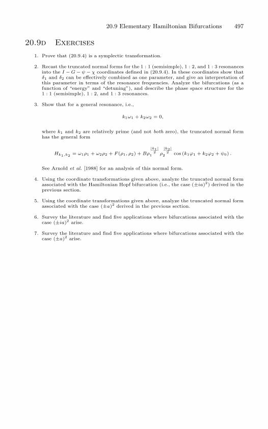
20.9 Elementary Hamiltonian Bifurcations 497
20.9d Exercises1. Prove that (20.9.4) is a symplectic transformation.
2. Recast the truncated normal forms for the 1 : 1 (semisimple), 1 : 2, and 1 : 3 resonancesinto the I − G − ψ − χ coordinates defined in (20.9.4). In these coordinates show thatδ1 and δ2 can be effectively combined as one parameter, and give an interpretation ofthis parameter in terms of the resonance frequencies. Analyze the bifurcations (as afunction of “energy” and “detuning”), and describe the phase space structure for the1 : 1 (semisimple), 1 : 2, and 1 : 3 resonances.
3. Show that for a general resonance, i.e.,
k1ω1 + k2ω2 = 0,
where k1 and k2 are relatively prime (and not both zero), the truncated normal formhas the general form
Hk1,k2 = ω1ρ1 + ω2ρ2 + F (ρ1, ρ2) + Bρ|k1|2
1 ρ|k2|2
2 cos (k1ϕ1 + k2ϕ2 + ψ0) .
See Arnold et al. [1988] for an analysis of this normal form.
4. Using the coordinate transformations given above, analyze the truncated normal formassociated with the Hamiltonian Hopf bifurcation (i.e., the case (±ia)2) derived in theprevious section.
5. Using the coordinate transformations given above, analyze the truncated normal formassociated with the case (±a)2 derived in the previous section.
6. Survey the literature and find five applications where bifurcations associated with thecase (±ia)2 arise.
7. Survey the literature and find five applications where bifurcations associated with thecase (±a)2 arise.
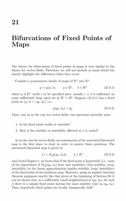
21
Bifurcations of Fixed Points ofMaps
The theory for bifurcations of fixed points of maps is very similar to thetheory for vector fields. Therefore, we will not include as much detail butmerely highlight the differences when they occur.
Consider a p-parameter family of maps of Rn into R
n
y → g(y, λ), y ∈ Rn, λ ∈ R
p (21.0.1)
where g is Cr (with r to be specified later, usually r ≥ 5 is sufficient) onsome sufficiently large open set in R
n × Rp. Suppose (21.0.1) has a fixed
point at (y, λ) = (y0, λ0), i.e.,
g(y0, λ0) = y0. (21.0.2)
Then, just as in the case for vector fields, two questions naturally arise.
1. Is the fixed point stable or unstable?
2. How is the stability or instability affected as λ is varied?
As in the case for vector fields, an examination of the associated linearizedmap is the first place to start in order to answer these questions. Theassociated linearized map is given by
ξ → Dyg(y0, λ0)ξ, ξ ∈ Rn, (21.0.3)
and, from Chapter 1, we know that if the fixed point is hyperbolic (i.e., noneof the eigenvalues of Dyg(y0, λ0) have unit modulus), then stability (resp.instability) in the linear approximation implies stability (resp. instability)of the fixed point of the nonlinear map. Moreover, using an implicit functiontheorem argument exactly like that given at the beginning of Section 20, itcan be shown that, in a sufficiently small neighborhood of (y0, λ0), for eachλ there is a unique fixed point having the same stability type as (y0, λ0).Thus, hyperbolic fixed points are locally dynamically dull!
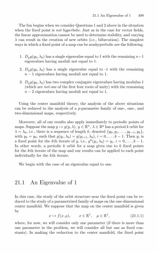
21.1 An Eigenvalue of 1 499
The fun begins when we consider Questions 1 and 2 above in the situationwhen the fixed point is not hyperbolic. Just as in the case for vector fields,the linear approximation cannot be used to determine stability, and varyingλ can result in the creation of new orbits (i.e., bifurcation). The simplestways in which a fixed point of a map can be nonhyperbolic are the following.
1. Dyg(y0, λ0) has a single eigenvalue equal to 1 with the remaining n−1eigenvalues having moduli not equal to 1.
2. Dyg(y0, λ0) has a single eigenvalue equal to -1 with the remainingn− 1 eigenvalues having moduli not equal to 1.
3. Dyg(y0, λ0) has two complex conjugate eigenvalues having modulus 1(which are not one of the first four roots of unity) with the remainingn− 2 eigenvalues having moduli not equal to 1.
Using the center manifold theory, the analysis of the above situationscan be reduced to the analysis of a p-parameter family of one-, one-, andtwo-dimensional maps, respectively.
Moreover, all of our results also apply immediately to periodic points ofmaps. Suppose the map y → g(y, λ), y ∈ R
n, λ ∈ Rp has a period k orbit for
λ = λ0, i.e., there is a sequence of length k, denoted y0, y1, . . . , yk−1, yk,with yk = y0, such that g(yi, λ0) = g(yi+1, λ0), i = 0, . . . , k − 1. Then yi isa fixed point for the kth iterate of g, i.e., gk(yi, λ0) = yi, i = 0, . . . , k − 1.In other words, a periodic k orbit for a map gives rise to k fixed pointsfor the kth iterate of the map and our results can be applied to each pointindividually for the kth iterate.
We begin with the case of an eigenvalue equal to one.
21.1 An Eigenvalue of 1
In this case, the study of the orbit structure near the fixed point can be re-duced to the study of a parametrized family of maps on the one-dimensionalcenter manifold. We suppose that the map on the center manifold is givenby
x → f(x, µ), x ∈ R1, µ ∈ R
1, (21.1.1)
where, for now, we will consider only one parameter (if there is more thanone parameter in the problem, we will consider all but one as fixed con-stants). In making the reduction to the center manifold, the fixed point
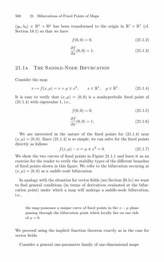
500 21. Bifurcations of Fixed Points of Maps
(y0, λ0) ∈ Rn × R
p has been transformed to the origin in R1 × R
1 (cf.Section 18.1) so that we have
f(0, 0) = 0, (21.1.2)
∂f
∂x(0, 0) = 1. (21.1.3)
21.1a The Saddle-Node Bifurcation
Consider the map
x → f(x, µ) = x + µ∓ x2, x ∈ R1, µ ∈ R
1. (21.1.4)
It is easy to verify that (x, µ) = (0, 0) is a nonhyperbolic fixed point of(21.1.4) with eigenvalue 1, i.e.,
f(0, 0) = 0, (21.1.5)
∂f
∂x(0, 0) = 1. (21.1.6)
We are interested in the nature of the fixed points for (21.1.4) near(x, µ) = (0, 0). Since (21.1.4) is so simple, we can solve for the fixed pointsdirectly as follows
f(x, µ)− x = µ∓ x2 = 0. (21.1.7)
We show the two curves of fixed points in Figure 21.1.1 and leave it as anexercise for the reader to verify the stability types of the different branchesof fixed points shown in this figure. We refer to the bifurcation occuring at(x, µ) = (0, 0) as a saddle-node bifurcation.
In analogy with the situation for vector fields (see Section 20.1c) we wantto find general conditions (in terms of derivatives evaluated at the bifur-cation point) under which a map will undergo a saddle-node bifurcation,i.e.,
the map possesses a unique curve of fixed points in the x − µ plane
passing through the bifurcation point which locally lies on one side
of µ = 0.
We proceed using the implicit function theorem exactly as in the case forvector fields.
Consider a general one-parameter family of one-dimensional maps
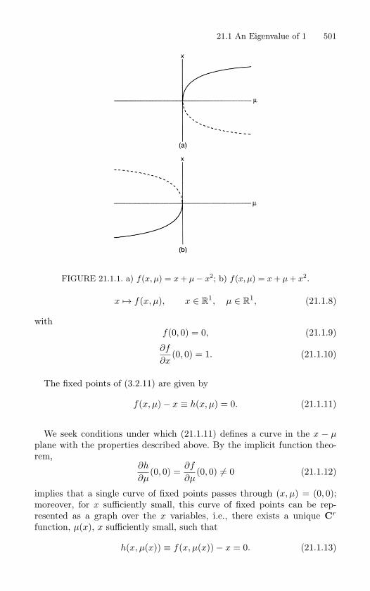
21.1 An Eigenvalue of 1 501
FIGURE 21.1.1. a) f(x, µ) = x + µ − x2; b) f(x, µ) = x + µ + x2.
x → f(x, µ), x ∈ R1, µ ∈ R
1, (21.1.8)
withf(0, 0) = 0, (21.1.9)
∂f
∂x(0, 0) = 1. (21.1.10)
The fixed points of (3.2.11) are given by
f(x, µ)− x ≡ h(x, µ) = 0. (21.1.11)
We seek conditions under which (21.1.11) defines a curve in the x − µplane with the properties described above. By the implicit function theo-rem,
∂h
∂µ(0, 0) =
∂f
∂µ(0, 0) = 0 (21.1.12)
implies that a single curve of fixed points passes through (x, µ) = (0, 0);moreover, for x sufficiently small, this curve of fixed points can be rep-resented as a graph over the x variables, i.e., there exists a unique Cr
function, µ(x), x sufficiently small, such that
h(x, µ(x)) ≡ f(x, µ(x))− x = 0. (21.1.13)
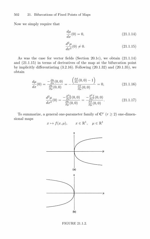
502 21. Bifurcations of Fixed Points of Maps
Now we simply require that
dµ
dx(0) = 0, (21.1.14)
d2µ
dx2 (0) = 0. (21.1.15)
As was the case for vector fields (Section 20.1c), we obtain (21.1.14)and (21.1.15) in terms of derivatives of the map at the bifurcation pointby implicitly differentiating (3.2.16). Following (20.1.32) and (20.1.35), weobtain
dµ
dx(0) =
−∂h∂x (0, 0)
∂h∂µ (0, 0)
= −
(∂f∂x (0, 0)− 1
)∂f∂µ (0, 0)
= 0, (21.1.16)
d2µ
dx2 (0) =−∂2h
∂x2 (0, 0)∂h∂µ (0, 0)
=−∂2f
∂x2 (0, 0)∂f∂µ (0, 0)
. (21.1.17)
To summarize, a general one-parameter family of Cr (r ≥ 2) one-dimen-sional maps
x → f(x, µ), x ∈ R1, µ ∈ R
1
FIGURE 21.1.2.
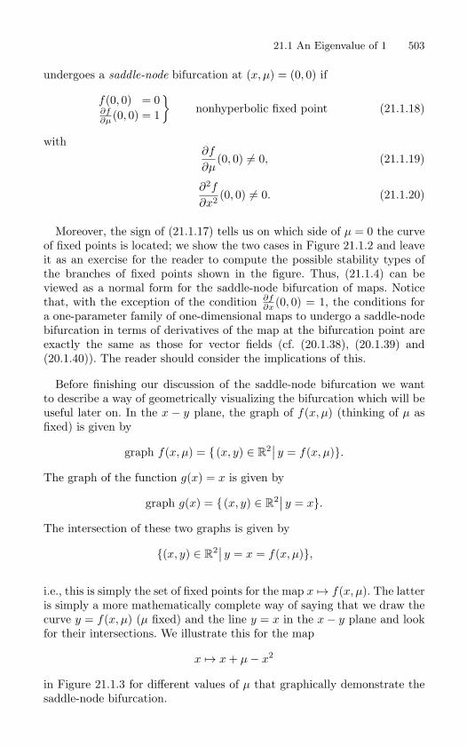
21.1 An Eigenvalue of 1 503
undergoes a saddle-node bifurcation at (x, µ) = (0, 0) if
f(0, 0) = 0∂f∂µ (0, 0) = 1
nonhyperbolic fixed point (21.1.18)
with∂f
∂µ(0, 0) = 0, (21.1.19)
∂2f
∂x2 (0, 0) = 0. (21.1.20)
Moreover, the sign of (21.1.17) tells us on which side of µ = 0 the curveof fixed points is located; we show the two cases in Figure 21.1.2 and leaveit as an exercise for the reader to compute the possible stability types ofthe branches of fixed points shown in the figure. Thus, (21.1.4) can beviewed as a normal form for the saddle-node bifurcation of maps. Noticethat, with the exception of the condition ∂f
∂x (0, 0) = 1, the conditions fora one-parameter family of one-dimensional maps to undergo a saddle-nodebifurcation in terms of derivatives of the map at the bifurcation point areexactly the same as those for vector fields (cf. (20.1.38), (20.1.39) and(20.1.40)). The reader should consider the implications of this.
Before finishing our discussion of the saddle-node bifurcation we wantto describe a way of geometrically visualizing the bifurcation which will beuseful later on. In the x − y plane, the graph of f(x, µ) (thinking of µ asfixed) is given by
graph f(x, µ) = (x, y) ∈ R2∣∣ y = f(x, µ).
The graph of the function g(x) = x is given by
graph g(x) = (x, y) ∈ R2∣∣ y = x.
The intersection of these two graphs is given by
(x, y) ∈ R2∣∣ y = x = f(x, µ),
i.e., this is simply the set of fixed points for the map x → f(x, µ). The latteris simply a more mathematically complete way of saying that we draw thecurve y = f(x, µ) (µ fixed) and the line y = x in the x− y plane and lookfor their intersections. We illustrate this for the map
x → x + µ− x2
in Figure 21.1.3 for different values of µ that graphically demonstrate thesaddle-node bifurcation.
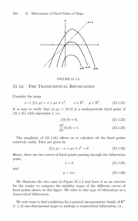
504 21. Bifurcations of Fixed Points of Maps
FIGURE 21.1.3.
21.1b The Transcritical Bifurcation
Consider the maps
x → f(x, µ) = x + µx∓ x2, x ∈ R1, µ ∈ R
1. (21.1.21)
It is easy to verify that (x, µ) = (0, 0) is a nonhyperbolic fixed point of(21.1.21) with eigenvalue 1, i.e.,
f(0, 0) = 0, (21.1.22)
∂f
∂x(0, 0) = 1. (21.1.23)
The simplicity of (21.1.21) allows us to calculate all the fixed pointsrelatively easily. They are given by
f(x, µ)− x = µx∓ x2 = 0. (21.1.24)
Hence, there are two curves of fixed points passing through the bifurcationpoint,
x = 0 (21.1.25)
andµ = ±x. (21.1.26)
We illustrate the two cases in Figure 21.1.4 and leave it as an exercisefor the reader to compute the stability types of the different curves offixed points shown in this figure. We refer to this type of bifurcation as atranscritical bifurcation.
We now want to find conditions for a general one-parameter family of Cr
(r ≥ 2) one-dimensional maps to undergo a transcritical bifurcation, i.e.,
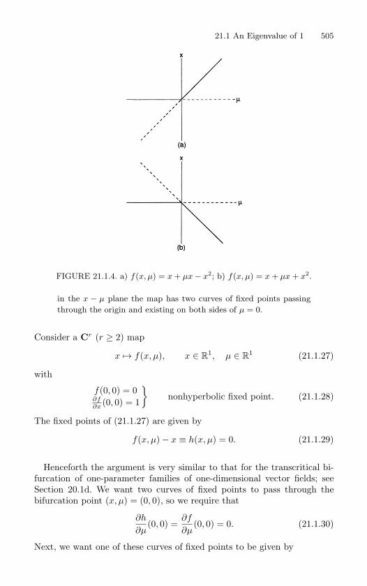
21.1 An Eigenvalue of 1 505
FIGURE 21.1.4. a) f(x, µ) = x + µx − x2; b) f(x, µ) = x + µx + x2.
in the x − µ plane the map has two curves of fixed points passing
through the origin and existing on both sides of µ = 0.
Consider a Cr (r ≥ 2) map
x → f(x, µ), x ∈ R1, µ ∈ R
1 (21.1.27)
with
f(0, 0) = 0∂f∂x (0, 0) = 1
nonhyperbolic fixed point. (21.1.28)
The fixed points of (21.1.27) are given by
f(x, µ)− x ≡ h(x, µ) = 0. (21.1.29)
Henceforth the argument is very similar to that for the transcritical bi-furcation of one-parameter families of one-dimensional vector fields; seeSection 20.1d. We want two curves of fixed points to pass through thebifurcation point (x, µ) = (0, 0), so we require that
∂h
∂µ(0, 0) =
∂f
∂µ(0, 0) = 0. (21.1.30)
Next, we want one of these curves of fixed points to be given by
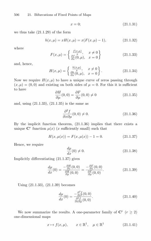
506 21. Bifurcations of Fixed Points of Maps
x = 0; (21.1.31)
we thus take (21.1.29) of the form
h(x, µ) = xH(x, µ) = x(F (x, µ)− 1), (21.1.32)
where
F (x, µ) =
f(x,µ)x , x = 0
∂f∂x (0, µ), x = 0
(21.1.33)
and, hence,
H(x, µ) =
h(x,µ)x , x = 0
∂h∂x (0, µ), x = 0
. (21.1.34)
Now we require H(x, µ) to have a unique curve of zeros passing through(x, µ) = (0, 0) and existing on both sides of µ = 0. For this it is sufficientto have
∂H
∂µ(0, 0) =
∂F
∂µ(0, 0) = 0 (21.1.35)
and, using (21.1.33), (21.1.35) is the same as
∂2f
∂x∂µ(0, 0) = 0. (21.1.36)
By the implicit function theorem, (21.1.36) implies that there exists aunique Cr function µ(x) (x sufficiently small) such that
H(x, µ(x)) = F (x, µ(x))− 1 = 0. (21.1.37)
Hence, we requiredµ
dx(0) = 0. (21.1.38)
Implicitly differentiating (21.1.37) gives
dµ
dx(0) =
−∂H∂x (0, 0)
∂H∂µ (0, 0)
=−∂F
∂x (0, 0)∂F∂µ (0, 0)
. (21.1.39)
Using (21.1.33), (21.1.39) becomes
dµ
dx(0) =
−∂2f∂x2 (0, 0)
∂2f∂x∂µ (0, 0)
. (21.1.40)
We now summarize the results. A one-parameter family of Cr (r ≥ 2)one-dimensional maps
x → f(x, µ), x ∈ R1, µ ∈ R
1 (21.1.41)
21.1 An Eigenvalue of 1 507
FIGURE 21.1.5.
a)(− ∂2f
∂x2 (0, 0)/ ∂2f∂x∂µ
(0, 0))
> 0;
b)(− ∂2f
∂x2 (0, 0)/ ∂2f∂x∂µ
(0, 0))
< 0.
having a nonhyperbolic fixed point, i.e.,
f(0, 0) = 0, (21.1.42)
∂f
∂x(0, 0) = 1, (21.1.43)
undergoes a transcritical bifurcation at (x, µ) = (0, 0) if
∂f
∂µ(0, 0) = 0, (21.1.44)
∂2f
∂x∂µ(0, 0) = 0, (21.1.45)
and∂2f
∂x2 (0, 0) = 0. (21.1.46)
We remark that the sign of (21.1.40) gives us the slope of the curve offixed points that is not x = 0. In Figure 21.1.5 we show the two cases andleave it as an exercise for the reader to compute the possible stability typesfor the different curves of fixed points shown in the figure; see Exercise
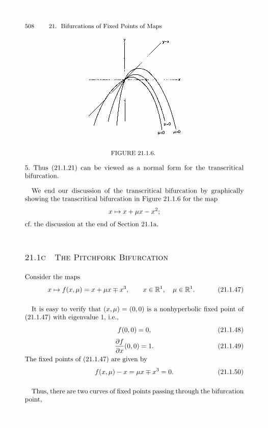
508 21. Bifurcations of Fixed Points of Maps
FIGURE 21.1.6.
5. Thus (21.1.21) can be viewed as a normal form for the transcriticalbifurcation.
We end our discussion of the transcritical bifurcation by graphicallyshowing the transcritical bifurcation in Figure 21.1.6 for the map
x → x + µx− x2;
cf. the discussion at the end of Section 21.1a.
21.1c The Pitchfork Bifurcation
Consider the maps
x → f(x, µ) = x + µx∓ x3, x ∈ R1, µ ∈ R
1. (21.1.47)
It is easy to verify that (x, µ) = (0, 0) is a nonhyperbolic fixed point of(21.1.47) with eigenvalue 1, i.e.,
f(0, 0) = 0, (21.1.48)
∂f
∂x(0, 0) = 1. (21.1.49)
The fixed points of (21.1.47) are given by
f(x, µ)− x = µx∓ x3 = 0. (21.1.50)
Thus, there are two curves of fixed points passing through the bifurcationpoint,
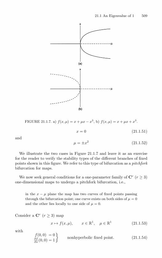
21.1 An Eigenvalue of 1 509
FIGURE 21.1.7. a) f(x, µ) = x + µx − x3, b) f(x, µ) = x + µx + x3.
x = 0 (21.1.51)
andµ = ±x2 (21.1.52)
We illustrate the two cases in Figure 21.1.7 and leave it as an exercisefor the reader to verify the stability types of the different branches of fixedpoints shown in this figure. We refer to this type of bifurcation as a pitchfork
bifurcation for maps.
We now seek general conditions for a one-parameter family of Cr (r ≥ 3)one-dimensional maps to undergo a pitchfork bifurcation, i.e.,
in the x − µ plane the map has two curves of fixed points passing
through the bifurcation point; one curve exists on both sides of µ = 0
and the other lies locally to one side of µ = 0.
Consider a Cr (r ≥ 3) map
x → f(x, µ), x ∈ R1, µ ∈ R
1 (21.1.53)
withf(0, 0) = 0∂f∂x (0, 0) = 1
nonhyperbolic fixed point. (21.1.54)
510 21. Bifurcations of Fixed Points of Maps
The fixed points of (21.1.53) are given by
f(x, µ)− x ≡ h(x, µ) = 0. (21.1.55)
Henceforth, the discussion is very similar to the discussion of the pitchforkbifurcation for vector fields (see Section 20.1). In order to have more thanone curve of fixed points passing through (x, µ) = (0, 0), we must have
∂h
∂µ(0, 0) =
∂f
∂µ(0, 0) = 0. (21.1.56)
Since we want one curve of fixed points to be x = 0, we take (21.1.55) ofthe form
h(x, µ) = xH(x, µ) = x(F (x, µ)− 1), (21.1.57)
where
H(x, µ) =
h(x,µ)x , x = 0
∂h∂x (0, µ), x = 0
(21.1.58)
and, hence,
F (x, µ) =
f(x,µ)x , x = 0
∂f∂x (0, µ), x = 0
. (21.1.59)
Since we want only one additional curve of fixed points to pass through(x, µ) = (0, 0), we require
∂H
∂µ(0, 0) =
∂F
∂µ(0, 0) = 0. (21.1.60)
Using (21.1.59), (21.1.60) becomes
∂2f
∂x∂µ(0, 0) = 0. (21.1.61)
The implicit function theorem and (21.1.61) imply that there is a uniqueCr function, µ(x) (x sufficiently small), such that
H(x, µ(x)) ≡ F (x, µ(x))− 1 = 0. (21.1.62)
We requiredµ
dx(0) = 0 (21.1.63)
andd2µ
dx2 (0) = 0. (21.1.64)
Implicitly differentiating (21.1.62) gives
21.1 An Eigenvalue of 1 511
dµ
dx(0) =
−∂H∂x (0, 0)
∂H∂µ (0, 0)
=−∂F
∂x (0, 0)∂F∂µ (0, 0)
, (21.1.65)
d2µ
dx2 (0) =−∂2H
∂x2 (0, 0)∂H∂µ (0, 0)
=−∂2F
∂x2 (0, 0)∂F∂µ (0, 0)
. (21.1.66)
Using (21.1.59), (21.1.65) and (21.1.66) become
dµ
dx(0) =
−∂2f∂x2 (0, 0)
∂2f∂x∂µ (0, 0)
, (21.1.67)
d2µ
dx2 (0) =−∂3f
∂x3 (0, 0)∂2f
∂x∂µ (0, 0). (21.1.68)
To summarize, a one-parameter family of Cr (r ≥ 3) one-dimensionalmaps
x → f(x, µ), x ∈ R1, µ ∈ R
1 (21.1.69)
having a nonhyperbolic fixed point, i.e.,
f(0, 0) = 0, (21.1.70)
∂f
∂x(0, 0) = 1, (21.1.71)
undergoes a pitchfork bifurcation at (x, µ) = (0, 0) if
∂f
∂µ(0, 0) = 0, (21.1.72)
∂2f
∂x2 (0, 0) = 0, (21.1.73)
∂2f
∂x∂µ(0, 0) = 0, (21.1.74)
∂3f
∂x3 (0, 0) = 0. (21.1.75)
Moreover, the sign of (21.1.68) tells us on which side of µ = 0 that oneof the curves of fixed points lies. We illustrate both cases in Figure 21.1.8and leave it as an exercise for the reader to compute the possible stabilitytypes of the different branches shown in Figure 21.1.8. Thus, we can view(21.1.47) as a normal form for the pitchfork bifurcation.
We end our discussion of the pitchfork bifurcation by graphically showingthe bifurcation for
x → x + µx− x3
in Figure 21.1.9 in the manner discussed at the end of Section 21.1a.
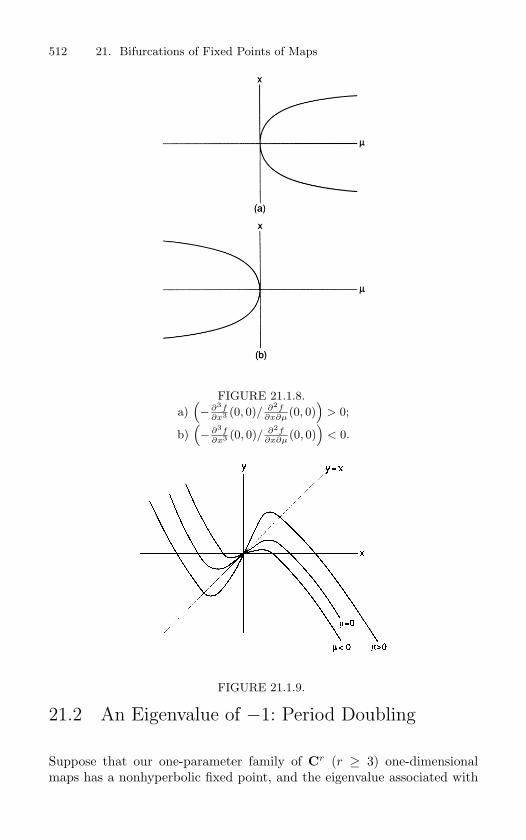
512 21. Bifurcations of Fixed Points of Maps
FIGURE 21.1.8.
a)(− ∂3f
∂x3 (0, 0)/ ∂2f∂x∂µ
(0, 0))
> 0;
b)(− ∂3f
∂x3 (0, 0)/ ∂2f∂x∂µ
(0, 0))
< 0.
FIGURE 21.1.9.
21.2 An Eigenvalue of −1: Period Doubling
Suppose that our one-parameter family of Cr (r ≥ 3) one-dimensionalmaps has a nonhyperbolic fixed point, and the eigenvalue associated with
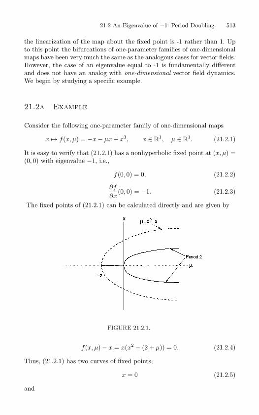
21.2 An Eigenvalue of −1: Period Doubling 513
the linearization of the map about the fixed point is -1 rather than 1. Upto this point the bifurcations of one-parameter families of one-dimensionalmaps have been very much the same as the analogous cases for vector fields.However, the case of an eigenvalue equal to -1 is fundamentally differentand does not have an analog with one-dimensional vector field dynamics.We begin by studying a specific example.
21.2a Example
Consider the following one-parameter family of one-dimensional maps
x → f(x, µ) = −x− µx + x3, x ∈ R1, µ ∈ R
1. (21.2.1)
It is easy to verify that (21.2.1) has a nonhyperbolic fixed point at (x, µ) =(0, 0) with eigenvalue −1, i.e.,
f(0, 0) = 0, (21.2.2)
∂f
∂x(0, 0) = −1. (21.2.3)
The fixed points of (21.2.1) can be calculated directly and are given by
FIGURE 21.2.1.
f(x, µ)− x = x(x2 − (2 + µ)) = 0. (21.2.4)
Thus, (21.2.1) has two curves of fixed points,
x = 0 (21.2.5)
and
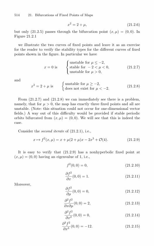
514 21. Bifurcations of Fixed Points of Maps
x2 = 2 + µ, (21.2.6)
but only (21.2.5) passes through the bifurcation point (x, µ) = (0, 0). InFigure 21.2.1
we illustrate the two curves of fixed points and leave it as an exercisefor the reader to verify the stability types for the different curves of fixedpoints shown in the figure. In particular we have
x = 0 is
unstable for µ ≤ −2,stable for − 2 < µ < 0,unstable for µ > 0,
(21.2.7)
and
x2 = 2 + µ is
unstable for µ ≥ −2,does not exist for µ < −2.
(21.2.8)
From (21.2.7) and (21.2.8) we can immediately see there is a problem,namely, that for µ > 0, the map has exactly three fixed points and all areunstable. (Note: this situation could not occur for one-dimensional vectorfields.) A way out of this difficulty would be provided if stable periodicorbits bifurcated from (x, µ) = (0, 0). We will see that this is indeed thecase.
Consider the second iterate of (21.2.1), i.e.,
x → f2(x, µ) = x + µ(2 + µ)x− 2x3 +O(4). (21.2.9)
It is easy to verify that (21.2.9) has a nonhyperbolic fixed point at(x, µ) = (0, 0) having an eigenvalue of 1, i.e.,
f2(0, 0) = 0, (21.2.10)
∂f2
∂x(0, 0) = 1. (21.2.11)
Moreover,∂f2
∂µ(0, 0) = 0, (21.2.12)
∂2f2
∂x∂µ(0, 0) = 2, (21.2.13)
∂2f2
∂x2 (0, 0) = 0, (21.2.14)
∂3f2
∂x3 (0, 0) = −12. (21.2.15)
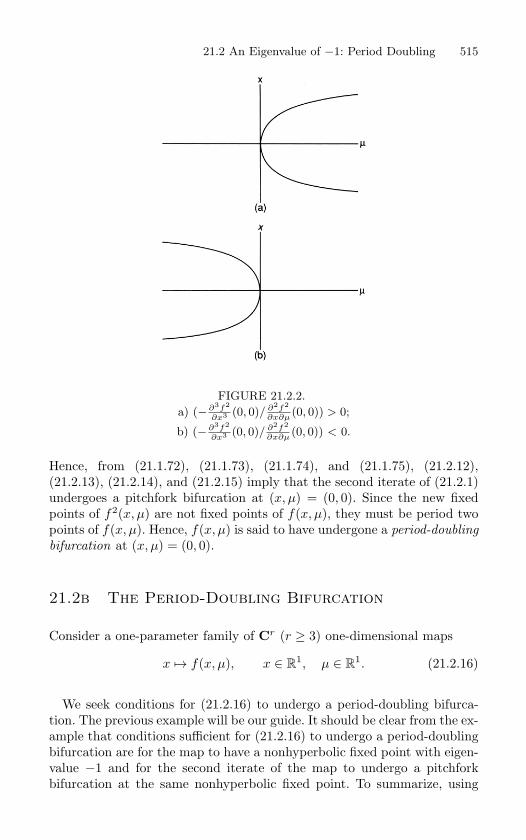
21.2 An Eigenvalue of −1: Period Doubling 515
FIGURE 21.2.2.
a) (− ∂3f2
∂x3 (0, 0)/ ∂2f2
∂x∂µ(0, 0)) > 0;
b) (− ∂3f2
∂x3 (0, 0)/ ∂2f2
∂x∂µ(0, 0)) < 0.
Hence, from (21.1.72), (21.1.73), (21.1.74), and (21.1.75), (21.2.12),(21.2.13), (21.2.14), and (21.2.15) imply that the second iterate of (21.2.1)undergoes a pitchfork bifurcation at (x, µ) = (0, 0). Since the new fixedpoints of f2(x, µ) are not fixed points of f(x, µ), they must be period twopoints of f(x, µ). Hence, f(x, µ) is said to have undergone a period-doubling
bifurcation at (x, µ) = (0, 0).
21.2b The Period-Doubling Bifurcation
Consider a one-parameter family of Cr (r ≥ 3) one-dimensional maps
x → f(x, µ), x ∈ R1, µ ∈ R
1. (21.2.16)
We seek conditions for (21.2.16) to undergo a period-doubling bifurca-tion. The previous example will be our guide. It should be clear from the ex-ample that conditions sufficient for (21.2.16) to undergo a period-doublingbifurcation are for the map to have a nonhyperbolic fixed point with eigen-value −1 and for the second iterate of the map to undergo a pitchforkbifurcation at the same nonhyperbolic fixed point. To summarize, using
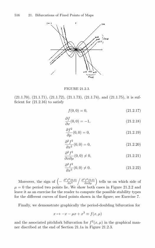
516 21. Bifurcations of Fixed Points of Maps
FIGURE 21.2.3.
(21.1.70), (21.1.71), (21.1.72), (21.1.73), (21.1.74), and (21.1.75), it is suf-ficient for (21.2.16) to satisfy
f(0, 0) = 0, (21.2.17)
∂f
∂x(0, 0) = −1, (21.2.18)
∂f2
∂µ(0, 0) = 0, (21.2.19)
∂2f2
∂x2 (0, 0) = 0, (21.2.20)
∂2f2
∂x∂µ(0, 0) = 0, (21.2.21)
∂3f2
∂x3 (0, 0) = 0. (21.2.22)
Moreover, the sign of(− ∂3f2(0,0)
∂x3
/∂2f2(0,0)
∂x∂µ
)tells us on which side of
µ = 0 the period two points lie. We show both cases in Figure 21.2.2 andleave it as an exercise for the reader to compute the possible stability typesfor the different curves of fixed points shown in the figure; see Exercise 7.
Finally, we demonstrate graphically the period-doubling bifurcation for
x → −x− µx + x3 ≡ f(x, µ)
and the associated pitchfork bifurcation for f2(x, µ) in the graphical man-ner discribed at the end of Section 21.1a in Figure 21.2.3.
21.3 A Pair of Eigenvalues of Modulus 1: The Naimark-Sacker Bifurcation 517
21.3 A Pair of Eigenvalues of Modulus 1: TheNaimark-Sacker Bifurcation
This section describes the map analog of the Poincare-Andronov-Hopf bi-furcation for vector fields but with some very different twists. Although thisbifurcation often goes by the name of “Hopf bifurcation for maps,” this ismisleading because the bifurcation theorem was first proved independentlyby Naimark [1959] and Sacker [1965]. Consequently, we will use the term“Naimark-Sacker bifurcation.”
We know that in this situation the study of the dynamics of (21.0.1) nearthe fixed point (y0, λ0) ∈ R
n × Rp can be reduced to the study of (21.0.1)
restricted to a p-parameter family of two-dimensional center manifolds. Weassume that the reduced map has been calculated and is given by
x → f(x, µ), x ∈ R2, µ ∈ R
1, (21.3.1)
where we take p = 1. If there is more than one parameter, we consider allbut one as fixed and denote it as µ. In restricting the map to the centermanifold, some preliminary transformations have been made so that thefixed point of (21.3.1) is given by (x, µ) = (0, 0), i.e., we have
f(0, 0) = 0, (21.3.2)
with the matrixDxf(0, 0) (21.3.3)
having two complex conjugate eigenvalues, denoted λ(0), λ(0), with
|λ(0)| = 1. (21.3.4)
We will also require that
λn(0) = 1, n = 1, 2, 3, 4. (21.3.5)
(Note: if λ(0) satisfies (21.3.5), then so does ¯λ(0), and vice versa.)
We showed in Example 19.3a that under these conditions a normal formfor (21.3.1) is given by
z → λ(µ)z + c(µ)z2z +O(4), z ∈ C, µ ∈ R1. (21.3.6)
We transform (21.3.6) into polar coordinates by letting
z = re2πiθ,
and obtain
518 21. Bifurcations of Fixed Points of Maps
r → |λ(µ)|(
r +(
Re(
c(µ)λ(µ)
))r3 +O(r4)
),
θ → θ + φ(µ) +12π
(Im
(c(µ)λ(µ)
))r2 +O(r3), (21.3.7)
where
φ(µ) ≡ 12π
tan−1 ω(µ)α(µ)
(21.3.8)
andc(µ) = α(µ) + iω(µ). (21.3.9)
We then Taylor expand the coefficients of (21.3.7) about µ = 0 and obtain
r →(
1 +d
dµ|λ(µ)|
∣∣∣∣µ=0
µ
)r +
(Re
(c(0)λ(0)
))r3 +O(µ2r, µr3, r4),
θ → θ + φ(0) +d
dµ(φ(µ))
∣∣∣∣µ=0
µ +12π
(Im
c(0)λ(0)
)r2
+O(µ2, µr2, r3), (21.3.10)
where we have used the condition that |λ(0)| = 1. Note that, since λn(0) =1, where n = 1, 2, 3, 4, from (21.3.8) we see that φ(0) = 0. We simplify thenotation associated with (21.3.10) by setting
d ≡ d
dµ|λ(µ)|
∣∣∣∣µ=0
,
a ≡ Re(
c(0)λ(0)
),
φ0 ≡ φ(0),
φ1 ≡d
dµ(φ(µ))
∣∣∣∣µ=0
,
b ≡ 12π
Imc(0)λ(0)
;
hence, (21.3.10) becomes
r → r + (dµ + ar2)r +O(µ2r, µr3, r4),θ → θ + φ0 + φ1µ + br2 +O(µ2, µr2, r3). (21.3.11)
We are interested in the dynamics of (21.3.11) for r small, µ small. Ourstrategy for understanding this will be the same as in our study of thePoincare-Andronov-Hopf bifurcation for vector fields (cf. Section 20.2);namely, we will study the dynamics of (21.3.11) with the higher order terms
neglected (i.e., the truncated normal form) and then try to understand how
21.3 A Pair of Eigenvalues of Modulus 1: The Naimark-Sacker Bifurcation 519
the dynamics of the truncated normal form are affected by the higher orderterms.
The truncated normal form is given by
r → r + (dµ + ar2)r,θ → θ + φ0 + φ1µ + br2. (21.3.12)
Note that r = 0 is a fixed point of (21.3.12) that is
asymptotically stable for dµ < 0,unstable for dµ > 0,unstable for µ = 0, a > 0,
andasymptotically stable for µ = 0, a < 0.
We recall our study of the truncated normal form for the Poincare-Andro-nov-Hopf bifurcation for vector fields (see Section 20.2). In that case, fixedpoints of the r component of the truncated normal form, with r > 0, corre-sponded to periodic orbits. Something geometrically (but not dynamically)similar happens for maps also.
Lemma 21.3.1
(r, θ) ∈ R+ × S1
∣∣ r =√
−µda
is a circle which is in-
variant under the dynamics generated by (21.3.12).
Proof: That this set of points is a circle is obvious. The fact that it isinvariant under the dynamics generated by (21.3.12) follows from the factthat the r coordinate of points starting on the circle do not change underiteration by (21.3.12).
It should be clear that the invariant circle can exist for either µ > 0or µ < 0 depending on the signs of d and a and that there will be onlyone invariant circle at a distance O(
õ) from the origin. Stability of the
invariant circle is determined by the sign of a. This is a new concept ofstability not previously discussed in this book, namely, the stability of aninvariant set. Its meaning, hopefully, is intuitively clear. The invariant circleis stable if initial conditions “sufficiently near” the circle stay near the circleunder all forward iterations by (21.3.12). It is asymptotically stable if thepoints actually approach the circle. We summarize this in the followinglemma.
Lemma 21.3.2 The invariant circle is asymptotically stable for a < 0 and
unstable for a > 0.
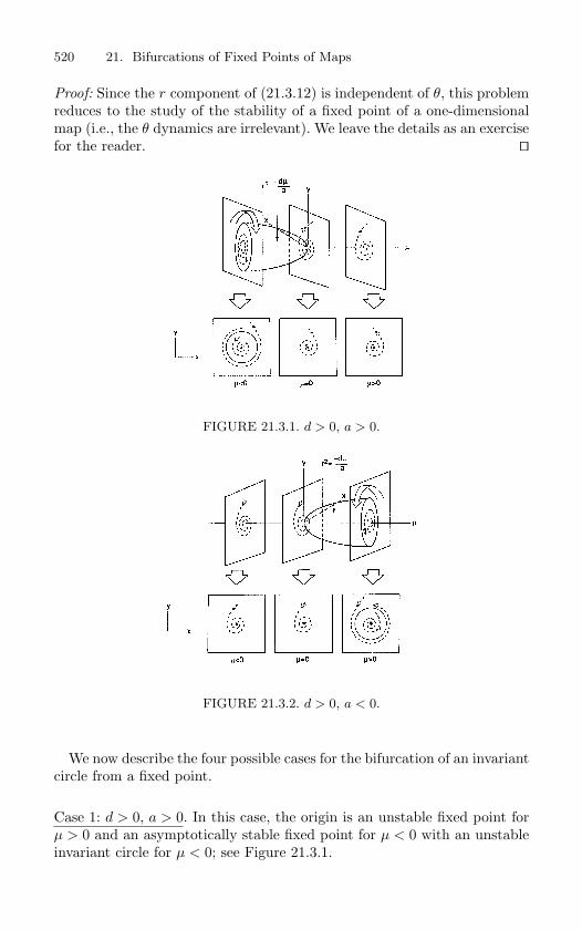
520 21. Bifurcations of Fixed Points of Maps
Proof: Since the r component of (21.3.12) is independent of θ, this problemreduces to the study of the stability of a fixed point of a one-dimensionalmap (i.e., the θ dynamics are irrelevant). We leave the details as an exercisefor the reader.
FIGURE 21.3.1. d > 0, a > 0.
FIGURE 21.3.2. d > 0, a < 0.
We now describe the four possible cases for the bifurcation of an invariantcircle from a fixed point.
Case 1: d > 0, a > 0. In this case, the origin is an unstable fixed point forµ > 0 and an asymptotically stable fixed point for µ < 0 with an unstableinvariant circle for µ < 0; see Figure 21.3.1.
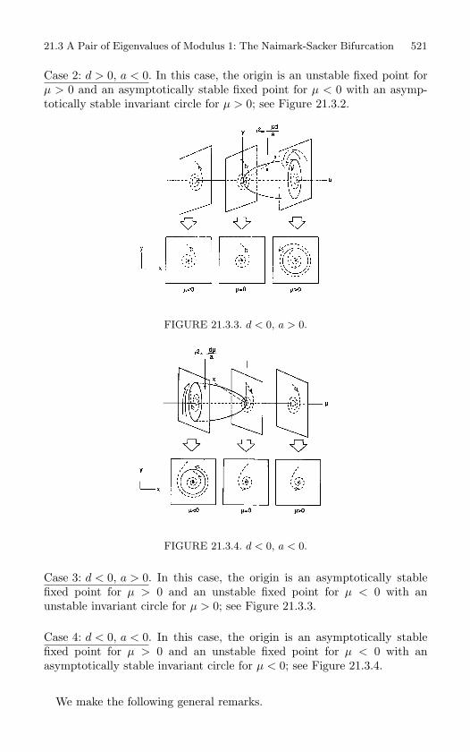
21.3 A Pair of Eigenvalues of Modulus 1: The Naimark-Sacker Bifurcation 521
Case 2: d > 0, a < 0. In this case, the origin is an unstable fixed point forµ > 0 and an asymptotically stable fixed point for µ < 0 with an asymp-totically stable invariant circle for µ > 0; see Figure 21.3.2.
FIGURE 21.3.3. d < 0, a > 0.
FIGURE 21.3.4. d < 0, a < 0.
Case 3: d < 0, a > 0. In this case, the origin is an asymptotically stablefixed point for µ > 0 and an unstable fixed point for µ < 0 with anunstable invariant circle for µ > 0; see Figure 21.3.3.
Case 4: d < 0, a < 0. In this case, the origin is an asymptotically stablefixed point for µ > 0 and an unstable fixed point for µ < 0 with anasymptotically stable invariant circle for µ < 0; see Figure 21.3.4.
We make the following general remarks.
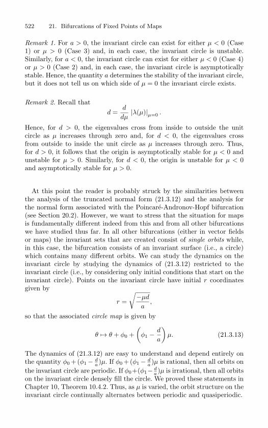
522 21. Bifurcations of Fixed Points of Maps
Remark 1. For a > 0, the invariant circle can exist for either µ < 0 (Case1) or µ > 0 (Case 3) and, in each case, the invariant circle is unstable.Similarly, for a < 0, the invariant circle can exist for either µ < 0 (Case 4)or µ > 0 (Case 2) and, in each case, the invariant circle is asymptoticallystable. Hence, the quantity a determines the stability of the invariant circle,but it does not tell us on which side of µ = 0 the invariant circle exists.
Remark 2. Recall thatd =
d
dµ|λ(µ)|µ=0 .
Hence, for d > 0, the eigenvalues cross from inside to outside the unitcircle as µ increases through zero and, for d < 0, the eigenvalues crossfrom outside to inside the unit circle as µ increases through zero. Thus,for d > 0, it follows that the origin is asymptotically stable for µ < 0 andunstable for µ > 0. Similarly, for d < 0, the origin is unstable for µ < 0and asymptotically stable for µ > 0.
At this point the reader is probably struck by the similarities betweenthe analysis of the truncated normal form (21.3.12) and the analysis forthe normal form associated with the Poincare-Andronov-Hopf bifurcation(see Section 20.2). However, we want to stress that the situation for mapsis fundamentally different indeed from this and from all other bifurcationswe have studied thus far. In all other bifurcations (either in vector fieldsor maps) the invariant sets that are created consist of single orbits while,in this case, the bifurcation consists of an invariant surface (i.e., a circle)which contains many different orbits. We can study the dynamics on theinvariant circle by studying the dynamics of (21.3.12) restricted to theinvariant circle (i.e., by considering only initial conditions that start on theinvariant circle). Points on the invariant circle have initial r coordinatesgiven by
r =
√−µd
a,
so that the associated circle map is given by
θ → θ + φ0 +(
φ1 −d
a
)µ. (21.3.13)
The dynamics of (21.3.12) are easy to understand and depend entirely onthe quantity φ0 +(φ1− d
a )µ. If φ0 +(φ1− da )µ is rational, then all orbits on
the invariant circle are periodic. If φ0+(φ1− da )µ is irrational, then all orbits
on the invariant circle densely fill the circle. We proved these statements inChapter 10, Theorem 10.4.2. Thus, as µ is varied, the orbit structure on theinvariant circle continually alternates between periodic and quasiperiodic.
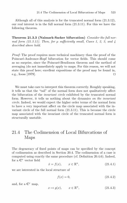
21.4 The Codimension of Local Bifurcations of Maps 523
Although all of this analysis is for the truncated normal form (21.3.12),our real interest is in the full normal form (21.3.11). For this we have thefollowing theorem.
Theorem 21.3.3 (Naimark-Sacker bifurcation) Consider the full nor-
mal form (21.3.11). Then, for µ sufficiently small, Cases 1, 2, 3, and 4
described above hold.
Proof: The proof requires more technical machinery than the proof of thePoincare-Andronov-Hopf bifurcation for vector fields. This should comeas no surprise, since the Poincare-Bendixson theorem and the method ofaveraging (do not immediately apply to maps. For this reason, we will notstate this proof here; excellent expositions of the proof may be found in,e.g., Iooss [1979].
We must take care to interpret this theorem correctly. Roughly speaking,it tells us that the “tail” of the normal form does not qualitatively affectthe bifurcation of the invariant circle exhibited by the truncated normalform. However, it tells us nothing about the dynamics on the invariant
circle. Indeed, we would expect the higher order terms of the normal formto have a very important affect on the circle map associated with the in-variant circle of the full normal form (21.3.11). This is because the circlemap associated with the invariant circle of the truncated normal form isstructurally unstable.
21.4 The Codimension of Local Bifurcations ofMaps
The degeneracy of fixed points of maps can be specified by the conceptof codimension as described in Section 20.4. The codimension of a case iscomputed using exactly the same procedure (cf. Definition 20.4.6). Indeed,for a Cr vector field
x = f(x), x ∈ Rn, (21.4.1)
we are interested in the local structure of
f(x) = 0, (21.4.2)
and, for a Cr map,x → g(x), x ∈ R
n, (21.4.3)
524 21. Bifurcations of Fixed Points of Maps
we are interested in the local structure of
g(x)− x = 0. (21.4.4)
Thus, it should be clear that, mathematically, (21.4.1) and (21.4.3) arethe same. We will, therefore, state the results for maps only and leave theverification to the reader.
21.4a One-Dimensional Maps
The mapsx → x + ax2 +O(x3), (21.4.5)
x → −x + ax3 +O(x4), (21.4.6)
have nonhyperbolic fixed points at x = 0. Using the techniques developedin Chapter 20, Section 20.4b it is easy to see that these are codimension
one fixed points with versal deformations given by
x → x + µ∓ x2, (21.4.7)
x → −x + µx∓ x3. (21.4.8)
Hence, the generic bifurcations of fixed points of one-parameter families ofone-dimensional maps are saddle-nodes and period-doublings.
Similarly, the mapx → x + ax3 +O(x4) (21.4.9)
has a nonhyperbolic fixed point at x = 0. It is easy to show that x = 0 isa codimension two fixed point, and a versal deformation is given by
x → x + µ1 + µ2x∓ x3. (21.4.10)
21.4b Two-Dimensional Maps
Suppose we have a two-dimensional map having a fixed point at the originwith the two eigenvalues of the associated linear map being complex con-jugates with modulus one. We denote the two eigenvalues by λ and λ. Onecan assign a codimension to this nonhyperbolic fixed point using the meth-ods of Section 20.4; the number obtained will depend on λ and λ (we will dothis shortly). We can then construct a candidate for a versal deformationusing the same methods. However, these will not give versal deformations.One of the obstructions to this involves the dynamics on invariant circles.As we have seen earlier (see Section 21.3), all of the higher order terms in
21.4 The Codimension of Local Bifurcations of Maps 525
the normal form may affect the dynamics on the invariant circle. Neverthe-less, we will give the codimension and the associated parametrized familiesusing the techniques of Section 20.4 for the different cases.
The caseλn = 1, n = 1, 2, 3, 4, (21.4.11)
is codimension one. The associated one-parameter family of normal formsfor this bifurcation is
z → (1 + µ)z + cz2z, z ∈ C (21.4.12)
(see Example 19.3a). If we ignore the dynamics on the invariant circle, then(21.4.12) captures all local dynamics.
The cases ruled out by (21.4.11) are referred to as the strong resonances.The cases n = 3 and n = 4 are codimension one with associated one-parameter families of normal forms given by
z → (1 + µ)z + c1z2 + c2z
2z, n = 3, z ∈ C, µ ∈ R1, (21.4.13)
z → (1 + µ)z + c1z3 + c2z
2z, n = 4, z ∈ C, µ ∈ R1. (21.4.14)
The cases n = 1 and n = 2 correspond to double 1 and double -1 eigenval-ues, respectively. If the matrices associated with the linear parts (in Jordancanonical form) are given by(
1 10 1
), n = 1, (21.4.15)
and (−1 10 −1
), n = 2, (21.4.16)
then these cases are codimension two with associated two-parameter fami-lies of normal forms given by
x → x + y,y → µ1 + µ2x + y + ax2 + bxy,
n = 1, (21.4.17)
x → x + y,y → µ1x + µ2y + y + ax3 + bx2y
n = 2. (21.4.18)
Arnold [1983] studied (21.4.13), (21.4.14), (21.4.17), and (21.4.18) in detailby using the important local technique of interpolating a discrete map bya flow. We will work out some of the details in the exercises. The stronglyresonant cases arise in applications in, for example, the situation of applyinga periodic external force to a system which would freely oscillate with agiven frequency. Strong resonance would occur when the forcing frequencyand natural frequency were commensurate in the ratios 1/1, 1/2, 1/3, and1/4. The surprising fact is that, in the cases n = 1 and n = 2, chaoticmotions of the Smale–horseshoe type (see Gambaudo [1985]) may arise.
526 21. Bifurcations of Fixed Points of Maps
21.5 Exercises
1. Verify the stability for the branches of fixed points of the maps (21.1.4) shown inFigure 21.1.1. For one dimensional maps (as opposed to one dimensional vector fields)period doubling bifurcations are possible, so this may limit the range in µ for whichthe stabilities indicated in Figure 21.1.1 are valid.
2. Verify the stability for the branches of fixed points of the maps (21.1.21) shown inFigure 21.1.4. For one dimensional maps (as opposed to one dimensional vector fields)period doubling bifurcations are possible, so this may limit the range in µ for whichthe stabilities indicated in Figure 21.1.4 are valid.
3. Verify the stability for the branches of fixed points of the maps (21.1.47) shown inFigure 21.1.7. For one dimensional maps (as opposed to one dimensional vector fields)period doubling bifurcations are possible, so this may limit the range in µ for whichthe stabilities indicated in Figure 21.1.7 are valid.
4. Consider the saddle-node bifurcation for maps and Figure 21.1.2. For the case(− ∂2f
∂x2 (0, 0)/ ∂f∂µ (0, 0)
)> 0, give conditions under which the upper part of the curve
of fixed points is stable and the lower part is unstable. Alternatively, give conditionsunder which the upper part of the curve of fixed points is unstable and the lower partis stable.
Repeat the exercise for the case(
− ∂2f
∂x2 (0, 0)/ ∂f∂µ (0, 0)
)< 0.
5. Consider the transcritical bifurcation for maps and Figure 21.1.5. For the case(− ∂2f
∂x2 (0, 0)/ ∂2f∂x∂µ (0, 0)
)> 0, give conditions for x = 0 to be stable for µ > 0 and
unstable for µ < 0. Alternatively, give conditions for x = 0 to be unstable for µ > 0and stable for µ < 0.
Repeat the exercise for the case(
− ∂2f
∂x2 (0, 0)/ ∂2f∂x∂µ (0, 0)
)< 0.
6. Consider the pitchfork bifurcation for maps and Figure 21.1.8. For the case(− ∂3f
∂x3 (0, 0)/ ∂2f∂x∂µ (0, 0)
)> 0, give conditions for x = 0 to be stable for µ > 0 and
unstable for µ < 0. Alternatively, give conditions for x = 0 to be unstable for µ > 0and stable for µ < 0.
Repeat the exercise for the case(
− ∂3f
∂x3 (0, 0)/ ∂2f∂x∂µ (0, 0)
)< 0.
7. Consider the period-doubling bifurcation for maps and Figure 21.2.2. For the case(− ∂3f2
∂x3 (0, 0)/ ∂2f2
∂x∂µ (0, 0))
> 0, give conditions for the period one points, x = 0, to bestable for µ > 0 and unstable for µ < 0. Alternatively, give conditions for x = 0 to beunstable for µ > 0 and stable for µ < 0.
Repeat the exercise for the case(
− ∂3f2
∂x3 (0, 0)/ ∂2f2
∂x∂µ (0, 0))
< 0.
8. In Exercise 6 in Chapter 18 we computed center manifolds near the origin for thefollowing one-parameter families of maps. Describe the bifurcations of the origin. In, forexample, a) and a′) the parameter ε multiplies a linear and nonlinear term, respectively.In terms of bifurcations, is there a qualitative difference in the two cases? What kindof general statements can you make?
a)x → − 1
2x − y − xy
2,
y → − 12
x + εy + x2,
(x, y) ∈ R2.
a′)x → − 1
2x − y − xy
2,
y → − 12
y + εy2 + x
2.
21.5 Exercises 527
b) x → x + 2y + x3,
y → 2x + y + εy,(x, y) ∈ R
2.
b′) x → x + 2y + x3,
y → 2x + y + εy2.
c) x → −x + y − xy2,
y → y + εy + x2y,
(x, y) ∈ R2.
c′) x → −x + y − xy2,
y → y + εy2 + x
2y.
d)x → 2x + y,
y → 2x + 3y + εx + x4,
(x, y) ∈ R2.
d′) x → 2x + y + εx2,
y → 2x + 3y + x4.
e)x → x + εy,
y → x + 2y + y2,
(x, y) ∈ R2.
e′) x → x + εy2,
y → x + 2y + y2.
f)x → 2x + 3y,
y → x + εy + x2 + xy
2,
(x, y) ∈ R2.
f′)x → 2x + 3y,
y → x + x2 + εy
2 + xy2.
g)
x → x − z3,
y → 2x − y + εy,
z → x +12
z + x3,
(x, y, z) ∈ R3.
g′)
x → x − z3,
y → 2x − y + εy2,
z → x +12
z + x3.
h)
x → x + εz4,
y → −x − 2y − x3,
z → y − 12
z + y2,
(x, y, z) ∈ R3.
h′)
x → x + εx + z4,
y → −x − 2y − x3,
z → y − 12
z + y2.
i) x → y + εx + x2,
y → y + xy,(x, y) ∈ R
2.
i′) x → y + x2,
y → y + xy + εx2.
j) x → εx + x2,
y → y + xy,(x, y) ∈ R
2.
j′) x → x2 + εy,
y → y + xy.
9. Center Manifolds at a Saddle-node Bifurcation Point for Maps
Following the discussion in Exercise 7 following Section 20.1, develop the center man-ifold theory for maps so that it applies at a saddle-node bifurcation point.
Apply the resulting theory to the following maps. In each case, compute the centermanifold and describe the dynamics near the origin for ε small. Discuss the bifurcationsthat occur (if any) at ε = 0.
528 21. Bifurcations of Fixed Points of Maps
a) x → ε + x + x2 − y
2,
y → x2 + y
2,
(x, y, ε) ∈ R3.
b) x → ε + εx + x2 − y
2,
y → x3 + y
2.
c) x → ε + x + x2 − y
2,
y → ε + x2 + y
2.
d)x → ε +
12
x − y − x2,
y → 12
x + y2.
e) x → ε − x + y + x3,
y → y + εx − x2.
f) x → ε + x + εx + y3,
y → x + 2y − x2.
g) x → ε − x + xy + y2,
y → 2x − xy − y2.
h) x → ε + 2x + y + x2y,
y → 12x + 3y − xy2.
10. For the Naimark–Sacker bifurcation, compute the expression for the coefficient a anal-ogous to (20.2.14) for vector field. (Hint: the answer can be found in Guckenheimerand Holmes [1983]).
11. Consider the following Cr (r ≥ 1) two-dimensional, time-periodic vector field
x = y,y = f(x, t), (x, y) ∈ R
2,
where f(x, t) has period T in t.
a) Show that the vector field has a (time-dependent) first integral and that thefirst integral is actually a Hamiltonian for the system.
b) Suppose that the vector field is (constantly) linearly damped as follows
x = y,y = −δy + f(x, t), δ > 0.
Show that the associated Poincare map cannot undergo Naimark–Sacker bifur-cations.
12. Consider a map of R2 having a fixed point at the origin where the eigenvalues associated
with the linearized map are complex conjugate and of unit modulus. We denote thetwo eigenvalues by λ and λ. The goal of this exercise is to study the dynamics nearthe origin in the cases
λq = 1, q = 1, 2, 3, 4.
We will begin by developing a very powerful local technique; namely, interpolating amap by a flow.
a) Prove the following lemma (Arnold [1983]).
Consider a Cr (r as large as necessary) mapping f : R2 → R
2 havinga fixed point at the origin with the eigenvalues of the linearizationat the origin given by e±2πip/q (and with a Jordan block of order2 if q = 1 or 2). In a sufficiently small neighborhood of the originthe iterate fq can be represented as follows
fq(z) = ϕ1(z) + O(|z|N ), z ∈ R
2,
21.5 Exercises 529
where ϕ1(z) is the time one map obtained from the flow generatedby a vector field, v(z). Moreover, the vector field is invariant underrotations about the origin through the angle 2π/q.
(Hint: first put fq in normal form
fq = Λz + F
r2 (z) + F
r3 (z) + · · · + F
rN−1(z) + O(|z|N ).
Next consider the vector field
z = (Λ − id)z + Fr2 (z) + F
r3 (z) + · · · + F
rN−1(z).)
Approximate the time one map of this vector field via Picard iteration (justifythe use of this method), and show that it gives the desired result. This will showwhy it is first necessary to put the map in normal form. Moser [1968] gives analternate proof of this lemma as well as a nice discussion of interpolation ofmaps by flows.
Next we must deal with versal deformations of these maps.
b) Prove the following lemma (Arnold [1983]).
Consider a deformation fλ, λ ∈ Rp, of a mapping f0 = f satisfy-
ing the hypotheses of the lemma in Part a). In a sufficiently smallneighborhood of the origin, the iterate fq
λ can be represented as
fqλ(z) = ϕ1,λ(z) + O(|z|N ), z ∈ R
2,
where ϕ1,λ(z) is the time one map obtained from the flow gener-ated by a vector field, vλ, that is invariant under rotations aboutthe origin through the angle 2π/q. Moreover, ϕ1,0(z) = ϕ1(z) andv0(z) = v(z).
(Hint: this lemma is a consequence of the fact that the normalizing transforma-tions, up to order N , depend differentiably on the parameters.)
c) A vector field on the plane may have1. Fixed points (hyperbolic and nonhyperbolic).2. Periodic orbits.3. Homoclinic orbits.4. Heteroclinic orbits.
Suppose the time one map of a vector field having all of these orbits approximatesthe map fq in the sense of the lemmas in Part a) and b). How would each ofthese orbits be affected by the higher order terms (i.e., the O(|z|N ) terms)?
Now we return to the main problem.
d) Show that the normal forms in the cases λq = 1, q = 1, 2, 3, 4, are given by
q = 1:x → x + y + · · · ,y → y + ax
2 + bxy + · · · ,(x, y) ∈ R
2.
q = 2:x → x + y + · · · ,y → y + ax
3 + bx2y + · · · ,
(x, y) ∈ R2.
q = 3: z → z + c1z2 + c2z2z + · · · , z ∈ C.
q = 4: z → z + c1z3 + c2z2z + · · · , z ∈ C.
e) Compute the codimension in each case. Argue that candidates for versal defor-mations are given by
q = 1:x → x + y,y → µ1 + µ2y + y + ax
2 + bxy,(x, y) ∈ R
2.
q = 2:x → x + y,y → µ1x + (1 + µ2)y + ax
3 + bx2y,
(x, y) ∈ R2.
q = 3: z → (1 + µ)z + c1z2 + c2z2z, z ∈ C.
q = 4: z → (1 + µ)z + c1z3 + c2z2z, z ∈ C.
530 21. Bifurcations of Fixed Points of Maps
f) Show that the vector fields that interpolate fq through the order given in Parte) are
q = 1: x = y,y = µ1 + µ2y + ax
2 + bxy,(x, y) ∈ R
2.
q = 2: x = y,y = µ1x + µ2y + ax
3 + bx2y,
(x, y) ∈ R2.
q = 3: z = µz + c1z2 + c2z2z, z ∈ C.
q = 4: z = µz + c1z3 + c2z2z, z ∈ C.
g) Describe the complete dynamics of each of the vector fields in Part f).
h) Using the results from Parts g) and c), describe the dynamics of fq near theorigin for q = 1, 2, 3, and 4.
We remark that the results of this problem were first obtained by Arnold [1977], [1983].A very interesting application to a vector field undergoing a Poincare–Andronov–Hopfbifurcation that is subjected to an external time-periodic perturbation can be foundin Gambaudo [1985].
13. Consider the following Cr (r as large as necessary) one-parameter family of vectorfields
x = f(x, µ), (x, µ) ∈ Rn × R
1.
Suppose this vector field has a fixed point at (x, µ) = (0, 0).
a) Suppose n = 1; can (x, µ) = (0, 0) undergo a period-doubling bifurcation?
b) Suppose n = 2; can (x, µ) = (0, 0) undergo a period-doubling bifurcation?
c) Suppose n = 3; can (x, µ) = (0, 0) undergo a period-doubling bifurcation?
(Hint: consider a linear vector field
x = Ax, x ∈ Rn
,
where the flow is given byx = e
Atx0,
and det eAt > 0 for finite t. Use these facts.)
21.6 Maps of the Circle
As we saw in the previous section, the Naimark-Sacker bifurcation gave riseto an invariant circle. Hence, the restriction of the map to the invariantcircle gives rise to a circle map. In this section we want to establish someof the basic properties of circle maps. First, we establish the setting andnotation.
We consider C1 orientation-preserving homeomorphisms of the circle, S1,into itself:
f : S1 → S1.
Our study of circle maps will be aided through the notion of a lift. Thisdevice will enable us to consider the circle map as defined on the real line
21.6 Maps of the Circle 531
(constructed from the periodic repetition of the unit interval), where issuessuch as differentiability and order preservation are straightforward. We nowdefine the lift of a circle map.
Definition 21.6.1 (The Lift of a Circle Map) Consider the following
map of the real line R to S1:
Π : R −→ S1,
x −→ e2πix ≡ θ.
The map F : R −→ R is said to be a lift of f : S1 −→ S1 if
Π F = f Π.
Through the lift, the property of orientation preservation is manifested byF being an increasing function of x, i.e, x1 > x2 implies F (x1) > F (x2).
Some authors choose to work with a circle of length one, others choose to
work with a circle of length 2π. The difference involves making sure the
appropriate factors of 2π are in the right places in the various formulae.
For example, in the map Π used in the definition of the lift the factor
2π in the exponent of the exponential implies that we are working on a
circle of length one.
We now consider some examples of lifts.
Example 21.6.1. Consider the circle map
f : S1 −→ S1,
θ −→ θ + 2πω.
Then, a lift F of the circle map f satisfies
f Π = e2πi(x+ω)= Π F = e2πiF (x),
from which it follows that,
F (x) = x + ω + k, where k is some integer.
End of Example 21.6.1
532 21. Bifurcations of Fixed Points of Maps
Example 21.6.2. Consider the circle map
f : S1 −→ S1,
θ −→ θ + ε sin θ.
Then, a lift F of the circle map f satisfies
f Π = e2πi(x+ ε2π
sin 2πx) = Π F = e2πiF (x)
from which it follows that,
F (x) = x +ε
2πsin 2πx + k, where k is some integer.
End of Example 21.6.2
A key quantity in describing the dynamics of circle maps is the rotation
number associated with a given circle map. We now develop a series oflemmas that will be used in proving some of the important properties ofthe rotation number.
The following lemma shows that two lifts of the same circle map differby an integer.
Lemma 21.6.2 Let f : S1 −→ S1 be an orientation preserving homeo-
morphism of the circle and let F1 and F2 be lifts of f . Then F1 = F2 + k,
where k is some integer.
Proof: The two lifts must satisfy
f Π = Π F1 = e2πiF1(x),
f Π = Π F2 = e2πiF2(x),
from which it follows immediately that F1 = F2 + k, where k is someinteger.
The following lemma shows that the iterate of the lift of a circle map isthe lift of the iterate of the circle map.
21.6 Maps of the Circle 533
Lemma 21.6.3 If F is a lift of f then Fn is a lift of fn, n ≥ 1.
Proof: By definition of a lift we have
Π F = f Π,
and therefore
Π F F = Π F 2 = f Π F = f f Π = f2 Π.
Repeating this argument establishes the result for arbitrary n.
Lemma 21.6.4 Let f : S1 −→ S1 be an orientation preserving homeo-
morphism of the circle and let F be a lift. Then
F (x + k) = F (x) + k
for any integer k.
Proof: We first consider the case k = 1.
Using the definition of the lift we have
e2πiF (x+1) = Π F (x+1) = f Π(x+1) = f Π(x) = Π F (x) = e2πiF (x).(21.6.1)
Thus,e2πiF (x+1) = e2πiF (x), (21.6.2)
which implies thatF (x + 1) = F (x) + j, (21.6.3)
where j is some integer. We now argue that j = 1.
We give a proof by contradiction that j = 1. Suppose that j > 1. Thensince F (x) is an increasing function there must exist a point, y, with x <y < x + 1, such that
F (y) = F (x) + m, 1 ≤ m < j.
Thenf Π(y) = e2πiF (y) = e2πiF (x) = f Π(x),
534 21. Bifurcations of Fixed Points of Maps
from which it follows thaty = x + m,
where m is some integer = 0. This contradicts our choice of y.
The case for a general integer k is proved similarly. We can replace x+1by x+k in (21.6.1). Then we can conclude that F (x+k) = F (x)+j, wherej is some integer. Applying the same argument allows us to conclude thatj = k.
Lemma 21.6.5 Let f : S1 −→ S1 be an orientation preserving homeo-
morphism of the circle and let F be a lift of f . Then Fn − id is a periodic
function with period one, n ≥ 1.
Proof: First prove the lemma for n = 1. Using Lemma 21.6.4, we have
F (x + 1)− (x + 1) = F (x)− x.
This proves the lemma for n = 1.
Now consider the case n > 1. By the chain rule, it follows that fn is alsoan orientation preserving homeomorphism of the circle, and by Lemma21.6.3 Fn is a lift of fn. Then using Lemma 21.6.4, it follows that
Fn(x + 1)− (x + 1) = Fn(x)− x.
This completes the proof of the lemma.
Lemma 21.6.6 Let f be an orientation preserving homeomorphism of the
circle with lift F . Then there exists an integer kn such that
kn < Fn(x)− x < kn + 3,
for every x ∈ R, n ≥ 1.
Proof: By Lemma 21.6.5, since Fn(x) − x is periodic with period 1, theresult will follow if it is established only for x ∈ [0, 1].
Now Fn(0) is between two integers m and m+1, i.e., m ≤ Fn(0) ≤ m+1.From Lemma 21.6.4 it then follows that m+1 ≤ Fn(1) ≤ m+2. Since F isincreasing it follows that m− 1 < Fn(x)− x < m + 2. If we let kn = m− 1the result follows.
21.6 Maps of the Circle 535
Lemma 21.6.7 Suppose f : S1 −→ S1 is an orientation preserving home-
omorphism and F is a lift. Then if |x−y| < 1, we have |Fn(x)−Fn(y)| < 1,n ≥ 1.
Proof: Now |x− y| < 1 implies that −1 < x− y < 1, or
1. x < 1 + y,
2. y < 1 + x.
Using Lemma 21.6.4, and the fact that F is increasing, we apply Fn toeach of these expressions to obtain
1. Fn(x) < Fn(1 + y) = Fn(y) + 1 ⇒ Fn(x)− Fn(y) < 1,
2. Fn(y) < Fn(1 + x) = Fn(x) + 1 ⇒ −1 < Fn(x)− Fn(y).
Which establishes the desired result.
We are now at the point where we can develop the definition of rotationnumber. For an orientation preserving homeomorphism f : S1 −→ S1, withF a lift of f , we define the quantity
ρ0(F ) ≡ limn→∞
|Fn(x)|n
.
First, we show that if this quantity exists, it is independent of x.
Lemma 21.6.8 If ρ0(F ) exists, then it is independent of x.
Proof: Let x and y be given points. Then y can be written in the form
y = y + k,
where k is an integer and |x − y| < 1. Using this representation for y, wehave
|Fn(x)− Fn(y)| = |Fn(x)− Fn(y + k)| = |Fn(x)− Fn(y)− k|,≤ |Fn(x)− Fn(y)|+ k.
536 21. Bifurcations of Fixed Points of Maps
Using Lemma 21.6.7, since |x− y| < 1 then |Fn(x)−Fn(y)| < 1. So we get
|Fn(x)− Fn(y)|n
≤ 1 + k
n,
and therefore
limn→∞
|Fn(x)− Fn(y)|n
= 0.
This completes the proof.
Example 21.6.3. Consider the circle map
f : S1 −→ S1
θ −→ θ + 2πω
with lift
F : R1 −→ R
1,
x −→ x + ω + k.
Then we have
ρ0(F ) = limn→∞
x + nω + nk
n= ω + k.
End of Example 21.6.3
Lemma 21.6.9 Let f : S1 −→ S1 be an orientation preserving homeo-
morphism and let F1 and F2 be lifts such that ρ0(F1) and ρ0(F2) exist.
Then ρ0(F1) = ρ0(F2) + k, where k is an integer.
Proof: From Lemma 21.6.2,
F1 = F2 + k.
Let Tk denote the translation map, i.e., Tk : x → x + k. Then we canrewrite this equation as
F1 = Tk F2.
Now we want to show that Tk commutes with F2. We have
F2 Tk = F2(x + k) = F2(x) + k, by Lemma 21.6.4,
21.6 Maps of the Circle 537
andTk F2(x) = F2(x) + k.
HenceF2 Tk = Tk F2.
We use this result in the following way. Since F1 = Tk F2 it follows that
Fn1 (x) = (Tk F2)
n (x),= (Tk F2) (Tk F2) · · · (Tk F2)(x)︸ ︷︷ ︸
n fold composition of Tk F2
,
= Fn2 Tn
k (x), where we have repeatedly commuted “pairwise,”Tk and F2
= Fn2 (x + nk),
= Fn2 (x) + nk, by Lemma 21.6.4.
HenceFn
1 = Fn2 + nk,
From which it immediately follows that
ρ0(F1) = ρ(F2) + k.
This completes the proof.
We now prove that ρ0(F ) exists.
Theorem 21.6.10 Let f : S1 −→ S1 be an orientation preserving home-
omorphism with lift F . Then
ρ0(F ) = limn→∞
|Fn(x)|n
exists and is independent of x.
Proof: We break the proof down into two cases.
Case 1:
Suppose f has a periodic point, i.e., there exists θ ∈ S1 such that fm(θ) =θ. Then
Fm(x) = x + k,
538 21. Bifurcations of Fixed Points of Maps
for some fixed x, where k is some integer. Therefore
F jm(x) = x + jk,
from which it follows that
limj→∞
|F jm(x)|jm
= limj→∞
x + jk
jm=
k
m.
Any integer n can be written in the form
n = jm + r, 0 ≤ r < m
and by Lemma 21.6.6 there exists a constant M such that
|F r(y)− y| ≤ M,
for all y ∈ R, 0 ≤ r < m. So we have
|Fn(x)− F jm(x)|n
=|F r(F jm(x))− F jm(x)|
n
≤ M
n,
from which it follows that
limn→∞
|Fn(x)|n
= limj→∞
|F jm(x)|jm + r
= limj→∞
x + jk
jm + r=
k
m.
So, ρ0(F ) exists whenever f has a periodic point, moreover, in this caseρ0(F ) is rational.
Case 2:
Now we consider the general case. By Lemma 21.6.6 there exists aninteger kn such that
kn < Fn(x)− x < kn + 3, (21.6.4)
for every x ∈ R, n ≥ 1. Applying (21.6.4) repeatedly to x = Fn(x), F 2n(x),· · ·, F (m−1)n(x), we get the following chain of inequalities
21.6 Maps of the Circle 539
kn < Fn(x)− x < kn + 3,
kn < F 2n(x)− Fn(x) < kn + 3,
kn < F 3n(x)− F 2n(x) < kn + 3,
...kn < Fmn(x)− F (m−1)n(x) < kn + 3.
Adding these inequalities gives
mkn < Fmn(x)− x < m(kn + 2),
or,kn
n<
Fmn(x)− x
mn<
kn + 3n
.
The first inequality in the chain of inequalities gives
kn
n<
Fn(0)n
<kn + 3
n.
Combining these two expressions gives the estimate∣∣∣∣Fmn(x)mn
− Fn(x)n
∣∣∣∣ <3n
(21.6.5)
Repeating the above argument with m and n interchanged gives∣∣∣∣Fmn(x)mn
− Fm(x)m
∣∣∣∣ <3m
(21.6.6)
Combining (21.6.5) and (21.6.6) gives∣∣∣∣Fn(x)n
− Fm(x)m
∣∣∣∣ <3
n + m.
Hence the sequence
F n(x)n
is a Cauchy sequence in R, so it converges.
Finally, we define the rotation number of an orientation preserving,homeomorphism of the circle.
Definition 21.6.11 (Rotation Number) There are two main opera-
tional definitions of rotation number. For f : S1 −→ S1 an orientation
preserving homeomorphism, with F a lift of f :
1. Some authors define the rotation number of f , denoted ρ(f), as the
fractional part of ρ0(F ) (e.g. Devaney [1986]).
540 21. Bifurcations of Fixed Points of Maps
2. Other authors define the rotation number of f to be ρ0(F ) (e.g., Katok
and Hasselblatt [1995]).
In either case, we have shown that the rotation number exists, and is inde-
pendent of the point x.
Next we show that that rotation number depends continuously on f inthe C0 topology.
Theorem 21.6.12 Let f : S1 −→ S1 be an orientation-preserving dif-
feomorphism. Let ε > 0 be given, then there exists a δ > 0 such that if
g : S1 −→ S1 is also an orientation preserving diffeomorphism which is
C0 − δ close to f then |ρ(f)− ρ(g)| < ε.
Proof: Choose n such that 3n < ε. From Lemma 21.6.6, there exists kn such
thatkn < Fn(0) < kn + 3
for F some lift of f . Choose δ sufficiently small so that for some lift G of gwe also have
kn < Gn(0) < kn + 3
Utilizing the same argument as in Theorem 21.6.10, we obtain the inequal-ities
kn
n<
Fmn(0)mn
<kn + 3
n
kn
n<
Gmn(0)mn
<kn + 3
n
Combining these inequalities gives∣∣∣∣Fmn(0)mn
− Gmn(0)mn
∣∣∣∣ <3n
< ε
and the result follows since
ρ0(F ) = limn→∞
=Fmn(0)
mn,
and
ρ0(G) = limn→∞
=Gmn(0)
mn,
and the limit is independent of the point.
21.6 Maps of the Circle 541
Theorem 21.6.13 The rotation number is irrational if and only if f has
no periodic points.
Proof: See Devaney [1986].
Theorem 21.6.14 The rotation number is rational if and only if f has a
periodic orbit.
Proof: In our proof of the existence of the rotation number we have shownthat if f has a periodic point, then the rotation number is rational. It re-mains to show that if the rotation number is rational, then f has a periodicpoint. We leave this to the exercises (or see Katok and Hasselblatt [1995]).
Here we introduce some terminology. Suppose the rotation number isrational, say p
q , with p and q relatively prime integers. We refer to theassociated periodic orbit as a “p − q” periodic orbit (or a periodic orbitof type “p − q”). In terms of the orbit of the point, it is a period q orbitthat makes p revolutions around the circle before returning to its originalstarting point.
The rotation number is invariant under orientation preserving topologicalconjugacy.
Theorem 21.6.15 Let f and g be orientation preserving homeomorphisms
of S1, then ρ(f) = ρ(g−1fg).
Proof: See Katok and Hasselblatt [1995].
The Rotation Number and Orbits
While we have seen that an orientation preserving circle homeomorphismhas periodic orbits if the rotation number is rational, and it has no periodicorbits if the rotation number is irrational, we have not characterized allpossible orbits for the two cases. This is done below, and is referred to asthe “Poincare classification” by Katok and Hasselblatt [1995], where theproof of the statements can be found.
542 21. Bifurcations of Fixed Points of Maps
Rational Rotation Number, pq
For any given initial condition, there are three possibilities for the orbit.
• A pq periodic orbit.
• A homoclinic orbit. The orbit asymptotically approaches a periodicorbit as n → −∞ and as n → +∞.
• A heteroclinic orbit. The orbit asymptotically approaches a periodicorbit as n → −∞ and a different periodic orbit as n → +∞.
Irrational Rotation Number
For any given initial condition, there are three possibilities for the orbit.
• An orbit that densely fills the circle.
• An orbit that densely fills a Cantor set on the circle.
• An orbit that is homoclinic to a Cantor set on the circle.
21.6a The Dynamics of a Special Class of CircleMaps-Arnold Tongues
The results above are rather general. Now we will study a more specificclass of circle maps and obtain more detailed information on the dynamics.In particular, we want to discuss the notion of phase locking and Arnoldtongues. The following discussion loosely follows Hall [1984].
Consider the following two-parameter family of C1 diffeomorphisms ofthe circle:
θ −→ 〈θ + φ + αγ(θ)〉
where 〈·〉 denotes the fractional part, and we have the following assumptionson γ : R
1 −→ R1
1. γ ∈ Cr, r ≥ 1,∣∣∣dγ
dθ
∣∣∣ ≤ 1,
2. ∀ θ ∈ R, γ(θ + 1) = γ(θ) + 1,
21.6 Maps of the Circle 543
3.1∫0
γ(θ)dθ = 0.
We will study the following lift of the above circle map:
f : θ −→ θ + φ + αγ(θ) ≡ f(θ, φ, α).
An example of a map of this type is given by
x → x + φ +α
2πsin 2πx,
which is often referred to as the standard map, which was studied in detailby Arnold [1965].
The two parameters are φ and α. For α = 0 the map is just a rigid, linearrotation through the angle φ. The parameter α controls the nonlinearity ofthe map.
We denote the rotation number of the lift by ρ(φ, α).
Theorem 21.6.16 For φ ∈ R, α ∈ [0, 1)
1. ρ(φ, α) exists and is independent of θ.
2. ρ(φ, α) is continuous in (φ, α) and nondecreasing in φ.
3. If ρ(φ, α) = pq , with p, q relatively prime positive integers, then there
exists θ ∈ [0, 1) such that fq(θ, φ, α) = θ + p.
Proof:
1. In order for this to be true we need only show that f is orientationpreserving and increasing, i.e., df
dθ > 0. We have
df
dθ(θ, φ, α) = 1 + α
dγ
dθ.
Since∣∣∣dγ
dθ
∣∣∣ ≤ 1 and α ∈ [0, 1) the result follows.
2. We have already established that ρ(φ, α) depends continuously onparameters (cf. Theorem 21.6.12).
544 21. Bifurcations of Fixed Points of Maps
We now show that ρ(φ, α) is nondecreasing in φ for each fixed α.
Fix α. For φ2 > φ1, we have
f(θ, φ2, α) = θ + φ2 + αγ(θ) > f(θ, φ1, α) = θ + φ1 + αγ(θ).
Thenfn(θ, φ2, α) > fn(θ, φ1, α),
from which it follows that
ρ(φ2, α) ≥ ρ(φ1, α).
3. Half of this result was established in Theorem 21.6.10, the other halfwas left as an exercise.
The following lemma will be useful.
Lemma 21.6.17 For any integer q,
fq(θ, φ, α) = θ + qφ + α
q−1∑j=0
γ(θ + jφ) + αh(θ, φ, α)
where h is as differentiable as γ and h → 0 as α → 0.
Proof: This just involves a direct calculation while introducing the correctnotation.
q = 1 : f(θ, φ, α) = θ + φ + γ(θ),q = 2 : f2(θ, φ, α) = θ + 2φ + αγ(θ) + αγ(θ + φ + αγ(θ)),q = 3 : f3(θ, φ, α) = θ + 3φ + αγ(θ) + αγ(θ + φ + αγ(θ))
+ αγ(θ + 2φ + α(γ(θ) + γ(θ + φ + αγ(θ)))).
Continuing in this manner, the qth iterate has the form
fq(θ, φ, α) = θ + qφ + α[γ(θ) + γ(θ + φ + αγ(θ)) + γ (θ + 2φ + α(γ(θ)
+ γ(θ + φ + αγ(θ))))+ γ (θ + 3φ + α(γ(θ) + γ(θ + φ + αγ(θ)) + γ(θ + 2φ + α(γ(θ)+ γ(θ + φ + αγ(θ)))))) + · · ·
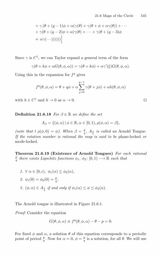
21.6 Maps of the Circle 545
+ γ (θ + (q − 1)φ + α(γ(θ) + γ(θ + φ + αγ(θ)) + · · ·+ γ(θ + (q − 2)φ + α(γ(θ) + · · ·+ γ(θ + (q − 3)φ
+ αγ(· · ·))))))]
Since γ is C1, we can Taylor expand a general term of the form
γ(θ + kφ + αG(θ, φ, α)) = γ(θ + kφ) + αγ′(ξ)G(θ, φ, α).
Using this in the expansion for fq gives
fq(θ, φ, α) = θ + qφ + α
q−1∑j=0
γ(θ + jφ) + αh(θ, φ, α)
with h ∈ C1 and h → 0 as α → 0.
Definition 21.6.18 For β ∈ R we define the set
Aβ = (φ, α) |φ ∈ R, α ∈ [0, 1), ρ(φ, α) = β,
(note that t ρ(φ, 0) = φ). When β = pq , A p
qis called an Arnold Tongue.
If the rotation number is rational the map is said to be phase-locked or
mode-locked.
Theorem 21.6.19 (Existence of Arnold Tongues) For each rationalpq there exists Lipschitz functions φ1, φ2: [0, 1) −→ R such that
1. ∀ α ∈ [0, ε), φ1(α) ≤ φ2(α),
2. φ1(0) = φ2(0) = pq ,
3. (φ, α) ∈ A pq
if and only if φ1(α) ≤ φ ≤ φ2(α).
The Arnold tongue is illustrated in Figure 21.6.1.
Proof: Consider the equation
G(θ, φ, α) ≡ fq(θ, φ, α)− θ − p = 0.
For fixed φ and α, a solution θ of this equation corresponds to a periodicpoint of period p
q . Now for α = 0, φ = pq is a solution, for all θ. We will use
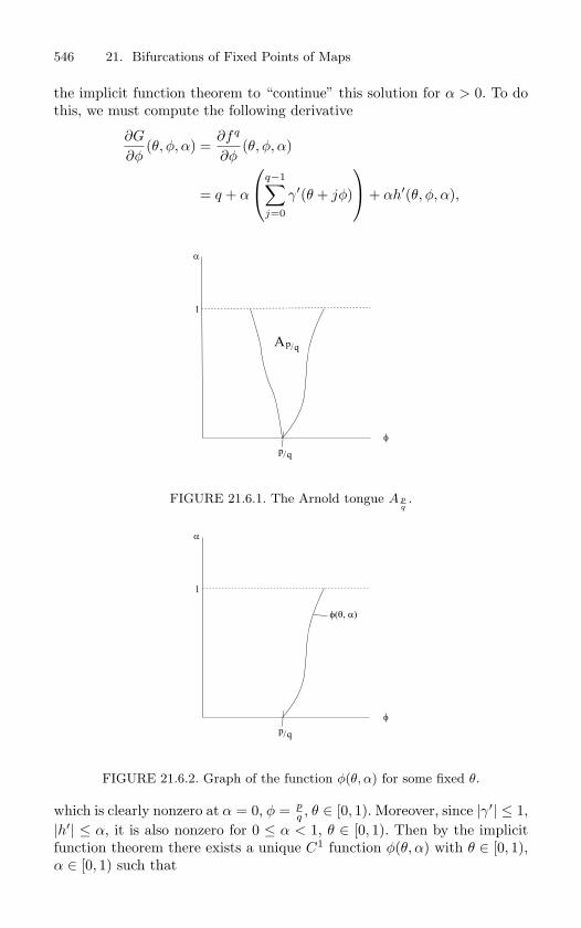
546 21. Bifurcations of Fixed Points of Maps
the implicit function theorem to “continue” this solution for α > 0. To dothis, we must compute the following derivative
∂G
∂φ(θ, φ, α) =
∂fq
∂φ(θ, φ, α)
= q + α
q−1∑
j=0
γ′(θ + jφ)
+ αh′(θ, φ, α),
p q/A
p q/
1
FIGURE 21.6.1. The Arnold tongue A pq.
p q/
1
FIGURE 21.6.2. Graph of the function φ(θ, α) for some fixed θ.
which is clearly nonzero at α = 0, φ = pq , θ ∈ [0, 1). Moreover, since |γ′| ≤ 1,
|h′| ≤ α, it is also nonzero for 0 ≤ α < 1, θ ∈ [0, 1). Then by the implicitfunction theorem there exists a unique C1 function φ(θ, α) with θ ∈ [0, 1),α ∈ [0, 1) such that
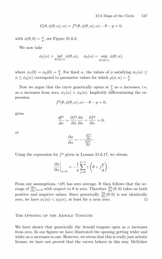
21.6 Maps of the Circle 547
G(θ, φ(θ, α), α) = fq(θ, φ(θ, α), α)− θ − p = 0,
with φ(θ, 0) = pq , see Figure 21.6.2.
We now take
φ1(α) = infθ∈[0,1)
φ(θ, α), φ2(α) = supθ∈[0,1)
φ(θ, α),
where φ1(0) = φ2(0) = pq . For fixed α, the values of φ satisfying φ1(α) ≤
φ ≤ φ2(α) correspond to parameter values for which ρ(φ, α) = pq .
Now we argue that the curve generically opens at pq as α increases, i.e,
as α increases from zero, φ1(α) < φ2(α). Implicitly differentiating the ex-pression
fq(θ, φ(θ, α), α)− θ − p = 0,
givesdfq
dα=
∂fq
∂φ
∂φ
∂α+
∂fq
∂α= 0,
or∂φ
∂α= −
∂fq
∂α∂fq
∂φ
.
Using the expression for fq given in Lemma 21.6.17, we obtain
∂φ
∂α
∣∣∣∣α=0
= −1q
q−1∑j=0
γ
(θ + j
p
q
).
From our assumptions, γ(θ) has zero average. It then follows that the av-erage of ∂φ
∂α |α=0 with respect to θ is zero. Therefore ∂φ∂α (θ, 0) takes on both
positive and negative values. Since generically ∂φ∂α (θ, 0) is not identically
zero, we have φ1(α) < φ2(α), at least for α near zero.
The Opening of the Arnold Tongues
We have shown that generically the Arnold tongues open as α increasesfrom zero. In our figures we have illustrated the opening getting wider andwider as α increases to one. However, we stress that this is really just artisticlicense; we have not proved that the curves behave in this way. McGehee
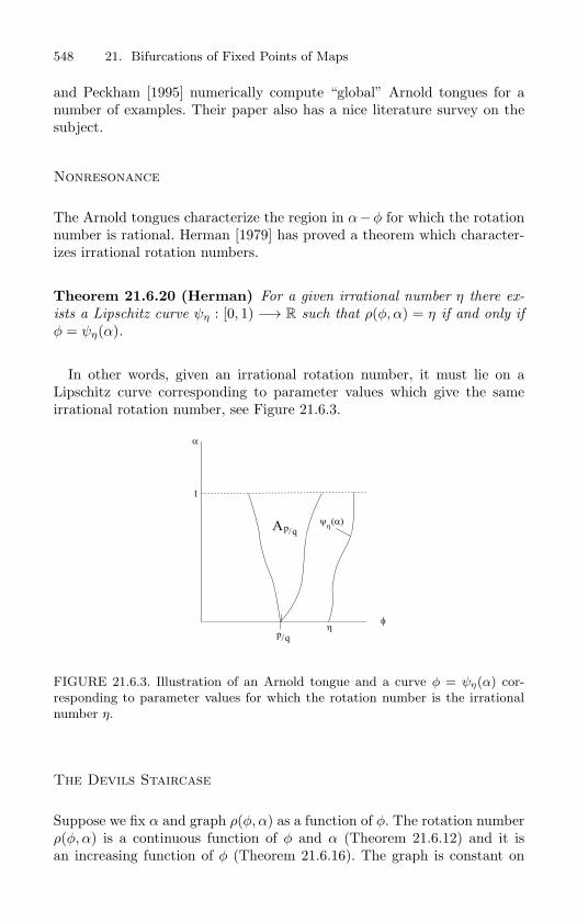
548 21. Bifurcations of Fixed Points of Maps
and Peckham [1995] numerically compute “global” Arnold tongues for anumber of examples. Their paper also has a nice literature survey on thesubject.
Nonresonance
The Arnold tongues characterize the region in α−φ for which the rotationnumber is rational. Herman [1979] has proved a theorem which character-izes irrational rotation numbers.
Theorem 21.6.20 (Herman) For a given irrational number η there ex-
ists a Lipschitz curve ψη : [0, 1) −→ R such that ρ(φ, α) = η if and only if
φ = ψη(α).
In other words, given an irrational rotation number, it must lie on aLipschitz curve corresponding to parameter values which give the sameirrational rotation number, see Figure 21.6.3.
p q/A
p q/
1
FIGURE 21.6.3. Illustration of an Arnold tongue and a curve φ = ψη(α) cor-
responding to parameter values for which the rotation number is the irrational
number η.
The Devils Staircase
Suppose we fix α and graph ρ(φ, α) as a function of φ. The rotation numberρ(φ, α) is a continuous function of φ and α (Theorem 21.6.12) and it isan increasing function of φ (Theorem 21.6.16). The graph is constant on
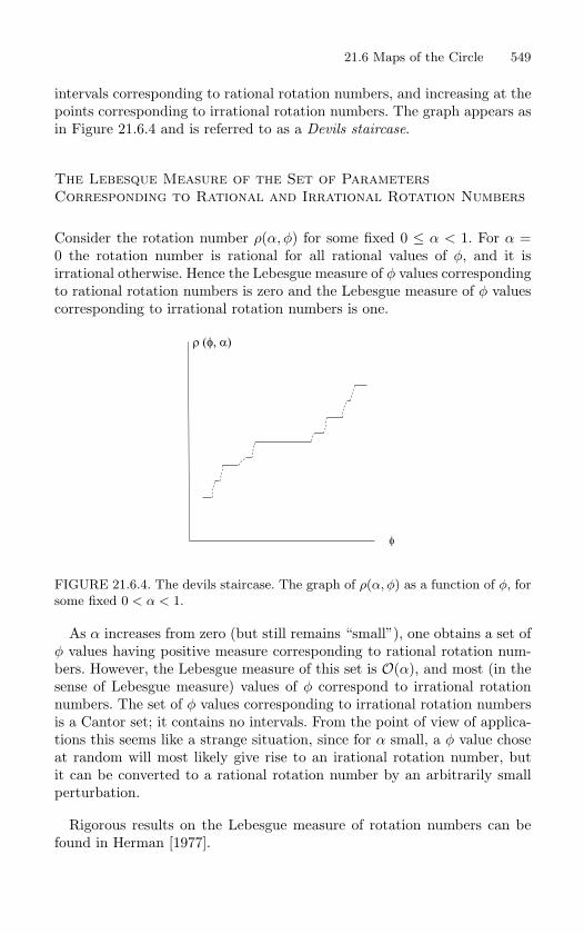
21.6 Maps of the Circle 549
intervals corresponding to rational rotation numbers, and increasing at thepoints corresponding to irrational rotation numbers. The graph appears asin Figure 21.6.4 and is referred to as a Devils staircase.
The Lebesque Measure of the Set of ParametersCorresponding to Rational and Irrational Rotation Numbers
Consider the rotation number ρ(α, φ) for some fixed 0 ≤ α < 1. For α =0 the rotation number is rational for all rational values of φ, and it isirrational otherwise. Hence the Lebesgue measure of φ values correspondingto rational rotation numbers is zero and the Lebesgue measure of φ valuescorresponding to irrational rotation numbers is one.
FIGURE 21.6.4. The devils staircase. The graph of ρ(α, φ) as a function of φ, for
some fixed 0 < α < 1.
As α increases from zero (but still remains “small”), one obtains a set ofφ values having positive measure corresponding to rational rotation num-bers. However, the Lebesgue measure of this set is O(α), and most (in thesense of Lebesgue measure) values of φ correspond to irrational rotationnumbers. The set of φ values corresponding to irrational rotation numbersis a Cantor set; it contains no intervals. From the point of view of applica-tions this seems like a strange situation, since for α small, a φ value choseat random will most likely give rise to an irational rotation number, butit can be converted to a rational rotation number by an arbitrarily smallperturbation.
Rigorous results on the Lebesgue measure of rotation numbers can befound in Herman [1977].
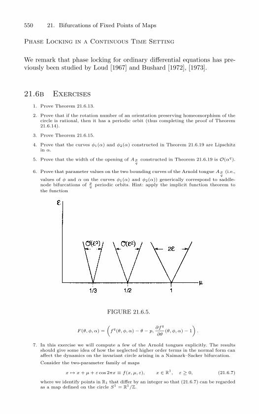
550 21. Bifurcations of Fixed Points of Maps
Phase Locking in a Continuous Time Setting
We remark that phase locking for ordinary differential equations has pre-viously been studied by Loud [1967] and Bushard [1972], [1973].
21.6b Exercises1. Prove Theorem 21.6.13.
2. Prove that if the rotation number of an orientation preserving homeomorphism of thecircle is rational, then it has a periodic orbit (thus completing the proof of Theorem21.6.14).
3. Prove Theorem 21.6.15.
4. Prove that the curves φ1(α) and φ2(α) constructed in Theorem 21.6.19 are Lipschitzin α.
5. Prove that the width of the opening of A pq
constructed in Theorem 21.6.19 is O(αq).
6. Prove that parameter values on the two bounding curves of the Arnold tongue A pq
(i.e.,
values of φ and α on the curves φ1(α) and φ2(α)) generically correspond to saddle-node bifurcations of p
q periodic orbits. Hint: apply the implicit function theorem tothe function
FIGURE 21.6.5.
F (θ, φ, α) =(
fq(θ, φ, α) − θ − p,
∂fq
∂θ(θ, φ, α) − 1
).
7. In this exercise we will compute a few of the Arnold tongues explicitly. The resultsshould give some idea of how the neglected higher order terms in the normal form canaffect the dynamics on the invariant circle arising in a Naimark–Sacker bifurcation.
Consider the two-parameter family of maps
x → x + µ + ε cos 2πx ≡ f(x, µ, ε), x ∈ R1, ε ≥ 0, (21.6.7)
where we identify points in R1 that differ by an integer so that (21.6.7) can be regardedas a map defined on the circle S1 = R
1/Z.
21.6 Maps of the Circle 551
a) Discuss the orbit structure of (21.6.7) for ε = 0. In particular, what is theLebesgue measure of the set of parameter values for which (21.6.7) has periodicorbits?
b) Consider the following regions in the µ − ε plane (see Figure 21.6.5).
µ = 1 ± ε,
µ =12
± ε2 π
2+ O(ε3),
µ =13
+ ε2
√3
6π ± ε
3√
7π
6+ O(ε4).
Show that, for parameter values in the interior of these regions, (21.6.7) has aperiod 1, period 2, and period 3 point, respectively.Hint: we outline the procedure for the period 2 points.
i. If x is a period 2 point of (21.6.7), then
f2(x, µ, ε) − x − 1 = G(x, µ, ε) = 0.
ii. If ∂G∂µ = 0, then we have a function µ = µ(x, ε) such that
G(x, µ(x, ε), ε) = 0. (21.6.8)
iii. Expand the function µ(x, ε) as follows
µ(x, ε) = µ(x, 0) + ε∂µ
∂ε(x, 0) +
ε2
2∂2µ
∂ε2(x, 0) + O(ε3).
iv. Implicitly differentiating (21.6.8), show that
µ(x, 0) =12
,
∂µ
∂ε(x, 0) = 0,
∂2µ
∂ε2(x, 0) = 2π sin 4πx.
v. Taking the infimum and supremum in Step 4, we obtain
µ = µ(x, ε) =12
± ε2 π
2+ O(ε3).
Justify all steps completely.Now let us return to the setting of the Naimark–Sacker bifurcation. For ε = 0,(21.6.7) has the form of the truncated Naimark–Sacker normal form restrictedto the invariant circle. The term ε cos 2πx could be viewed as illustrating thepossible effects of higher order terms in the normal form. For (21.6.7), at ε = 0the map has periodic orbits for all rational µ (i.e., a set of Lebesgue measurezero). For ε small and fixed, our results show that the measure of the set of µvalues for which (21.6.7) has a periodic orbit is positive. Thus, based on thisexample, we might expect the higher order terms in the Naimark–Sacker normalform to have a dramatic influence on the dynamics restricted to the bifurcatedinvariant circle. See Iooss [1979] for more details.
8. For some fixed 0 < ε < 1, compute the devils staircase for the following map
x → x + µ + ε cos 2πx ≡ f(x, µ, ε),
where x ∈ R1.
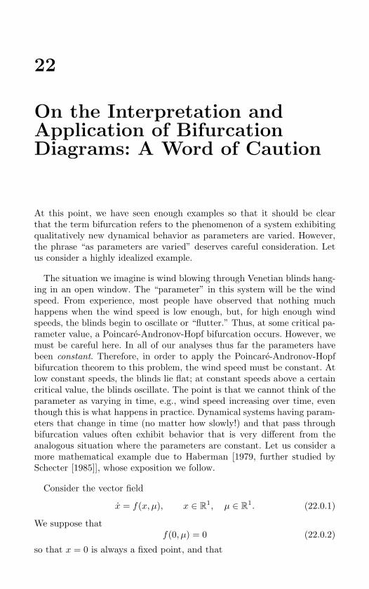
22
On the Interpretation andApplication of BifurcationDiagrams: A Word of Caution
At this point, we have seen enough examples so that it should be clearthat the term bifurcation refers to the phenomenon of a system exhibitingqualitatively new dynamical behavior as parameters are varied. However,the phrase “as parameters are varied” deserves careful consideration. Letus consider a highly idealized example.
The situation we imagine is wind blowing through Venetian blinds hang-ing in an open window. The “parameter” in this system will be the windspeed. From experience, most people have observed that nothing muchhappens when the wind speed is low enough, but, for high enough windspeeds, the blinds begin to oscillate or “flutter.” Thus, at some critical pa-rameter value, a Poincare-Andronov-Hopf bifurcation occurs. However, wemust be careful here. In all of our analyses thus far the parameters havebeen constant. Therefore, in order to apply the Poincare-Andronov-Hopfbifurcation theorem to this problem, the wind speed must be constant. Atlow constant speeds, the blinds lie flat; at constant speeds above a certaincritical value, the blinds oscillate. The point is that we cannot think of theparameter as varying in time, e.g., wind speed increasing over time, eventhough this is what happens in practice. Dynamical systems having param-eters that change in time (no matter how slowly!) and that pass throughbifurcation values often exhibit behavior that is very different from theanalogous situation where the parameters are constant. Let us consider amore mathematical example due to Haberman [1979, further studied bySchecter [1985]], whose exposition we follow.
Consider the vector field
x = f(x, µ), x ∈ R1, µ ∈ R
1. (22.0.1)
We suppose thatf(0, µ) = 0 (22.0.2)
so that x = 0 is always a fixed point, and that
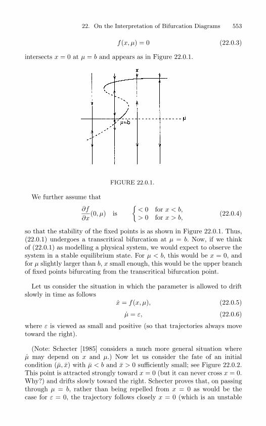
22. On the Interpretation of Bifurcation Diagrams 553
f(x, µ) = 0 (22.0.3)
intersects x = 0 at µ = b and appears as in Figure 22.0.1.
FIGURE 22.0.1.
We further assume that
∂f
∂x(0, µ) is
< 0 for x < b,> 0 for x > b, (22.0.4)
so that the stability of the fixed points is as shown in Figure 22.0.1. Thus,(22.0.1) undergoes a transcritical bifurcation at µ = b. Now, if we thinkof (22.0.1) as modelling a physical system, we would expect to observe thesystem in a stable equilibrium state. For µ < b, this would be x = 0, andfor µ slightly larger than b, x small enough, this would be the upper branchof fixed points bifurcating from the transcritical bifurcation point.
Let us consider the situation in which the parameter is allowed to driftslowly in time as follows
x = f(x, µ), (22.0.5)
µ = ε, (22.0.6)
where ε is viewed as small and positive (so that trajectories always movetoward the right).
(Note: Schecter [1985] considers a much more general situation whereµ may depend on x and µ.) Now let us consider the fate of an initialcondition (µ, x) with µ < b and x > 0 sufficiently small; see Figure 22.0.2.This point is attracted strongly toward x = 0 (but it can never cross x = 0.Why?) and drifts slowly toward the right. Schecter proves that, on passingthrough µ = b, rather than being repelled from x = 0 as would be thecase for ε = 0, the trajectory follows closely x = 0 (which is an unstable
554 22. On the Interpretation of Bifurcation Diagrams
invariant manifold for µ > b) for awhile before ultimately being repelledaway; see Figure 22.0.2.
FIGURE 22.0.2.
Thus, what one would observe for ε = 0 differs from that for ε = 0; forε = 0, certain trajectories tend to remain in the neighborhood (for awhile)of what are unstable fixed points for ε = 0.
A detailed analysis of problems of this type is beyond the scope of thisbook (such problems fit very nicely into the context of singular perturba-tion theory). The point we wish to make is that, within a given system,the behavior of that system on either side of a bifurcation value may bevery different in cases when the parameter varies slowly in time (no matterhow slowly) through the bifurcation value, as opposed to cases when theparameter is constant. “Slowly varying” saddle-node, transcritical, pitch-fork, and Hopf bifurcations for vector fields have all been considered, aswell as their Hamiltonian analogs. The reader will find detailed analysesof such problems in Mitropol’skii [1965], Lebovitz and Schaar [1975, 1977],Haberman [1979], Neishtadt [1987], [1988], Baer et al. [1989], Erneux andMandel [1986], Lebovitz and Pesci [1995], and Raman and Bajaj [1998] .The recent review of Arnold et al. [1994] provides an overview of manyof the latest results in this area. Baesens [1991], [1995] considers similarphenomena in maps.
23
The Smale Horseshoe
We will begin our study of “chaotic dynamics” by describing and analyzinga two-dimensional map possessing an invariant set having a delightfullycomplicated structure. The discussion is virtually the same as the discussionin Wiggins [1988]. Our map is a simplified version of a map first studiedby Smale [1963], [1980] and, due to the shape of the image of the domainof the map, is called a Smale horseshoe.
We will see that the Smale horseshoe is the prototypical map possess-ing a chaotic invariant set (note: the phrase “chaotic invariant set” willbe precisely defined later on in the discussion). Therefore, we feel that athorough understanding of the Smale horseshoe is absolutely essential forunderstanding what is meant by the term “chaos” as it is applied to thedynamics of specific physical systems. For this reason we will first endeavorto define as simple a two-dimensional map as possible that still containsthe necessary ingredients for possessing a complicated and chaotic dynam-ical structure so that the reader may get a feel for what is going on in themap with a minimum of distractions. As a result, our construction may notappeal to those interested in applications, since it may appear rather arti-ficial. However, following our discussion of the simplified Smale horseshoemap, we will give sufficient conditions for the existence of Smale horseshoe–like dynamics in two-dimensional maps that are of a very general nature.We will begin by defining the map and then proceed to a geometrical con-struction of the invariant set of the map. We will utilize the nature of thegeometrical construction in such a way as to motivate a description of thedynamics of the map on its invariant set by symbolic dynamics, followingwhich we will make precise the idea of chaotic dynamics.
23.1 Definition of the Smale Horseshoe Map
We will give a combination geometrical-analytical definition of the map.Consider a map, f , from the square having sides of unit length into R
2
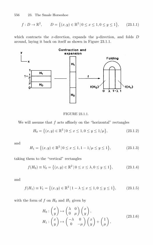
556 23. The Smale Horseshoe
f : D → R2, D =
(x, y) ∈ R
2 | 0 ≤ x ≤ 1, 0 ≤ y ≤ 1, (23.1.1)
which contracts the x-direction, expands the y-direction, and folds Daround, laying it back on itself as shown in Figure 23.1.1.
FIGURE 23.1.1.
We will assume that f acts affinely on the “horizontal” rectangles
H0 =(x, y) ∈ R
2 | 0 ≤ x ≤ 1, 0 ≤ y ≤ 1/µ, (23.1.2)
andH1 =
(x, y) ∈ R
2 | 0 ≤ x ≤ 1, 1− 1/µ ≤ y ≤ 1, (23.1.3)
taking them to the “vertical” rectangles
f(H0) ≡ V0 =(x, y) ∈ R
2 | 0 ≤ x ≤ λ, 0 ≤ y ≤ 1, (23.1.4)
and
f(H1) ≡ V1 =(x, y) ∈ R
2 | 1− λ ≤ x ≤ 1, 0 ≤ y ≤ 1, (23.1.5)
with the form of f on H0 and H1 given by
H0 :(
xy
)→
(λ 00 µ
)(xy
),
H1 :(
xy
)→
(−λ 00 −µ
)(xy
)+
(1µ
),
(23.1.6)
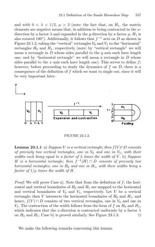
23.1 Definition of the Smale Horseshoe Map 557
and with 0 < λ < 1/2, µ > 2 (note: the fact that, on H1, the matrixelements are negative means that, in addition to being contracted in the x-direction by a factor λ and expanded in the y-direction by a factor µ, H1 isalso rotated 180). Additionally, it follows that f−1 acts on D as shown inFigure 23.1.2, taking the “vertical” rectangles V0 and V1 to the “horizontal”rectangles H0 and H1, respectively (note: by “vertical rectangle” we willmean a rectangle in D whose sides parallel to the y axis each have lengthone, and by “horizontal rectangle” we will mean a rectangle in D whosesides parallel to the x axis each have length one). This serves to define f ;however, before proceeding to study the dynamics of f on D, there is aconsequence of the definition of f which we want to single out, since it willbe very important later.
FIGURE 23.1.2.
Lemma 23.1.1 a) Suppose V is a vertical rectangle; then f(V )∩D consists
of precisely two vertical rectangles, one in V0 and one in V1, with their
widths each being equal to a factor of λ times the width of V . b) Suppose
H is a horizontal rectangle; then f−1(H) ∩ D consists of precisely two
horizontal rectangles, one in H0 and one in H1, with their widths being a
factor of 1/µ times the width of H.
Proof: We will prove Case a). Note that from the definition of f , the hori-zontal and vertical boundaries of H0 and H1 are mapped to the horizontaland vertical boundaries of V0 and V1, respectively. Let V be a verticalrectangle; then V intersects the horizontal boundaries of H0 and H1, andhence, f(V ) ∩ D consists of two vertical rectangles, one in V0 and one inV1. The contraction of the width follows from the form of f on H0 and H1,which indicates that the x-direction is contracted uniformly by a factor λon H0 and H1. Case b) is proved similarly. See Figure 23.1.3.
We make the following remarks concerning this lemma.
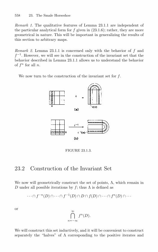
558 23. The Smale Horseshoe
Remark 1. The qualitative features of Lemma 23.1.1 are independent ofthe particular analytical form for f given in (23.1.6); rather, they are moregeometrical in nature. This will be important in generalizing the results ofthis section to arbitrary maps.
Remark 2. Lemma 23.1.1 is concerned only with the behavior of f andf−1. However, we will see in the construction of the invariant set that thebehavior described in Lemma 23.1.1 allows us to understand the behaviorof fn for all n.
We now turn to the construction of the invariant set for f .
FIGURE 23.1.3.
23.2 Construction of the Invariant Set
We now will geometrically construct the set of points, Λ, which remain inD under all possible iterations by f ; thus Λ is defined as
· · · ∩ f−n(D) ∩ · · · ∩ f−1(D) ∩D ∩ f(D) ∩ · · · ∩ fn(D) ∩ · · ·
or ∞⋂n=−∞
fn(D).
We will construct this set inductively, and it will be convenient to constructseparately the “halves” of Λ corresponding to the positive iterates and
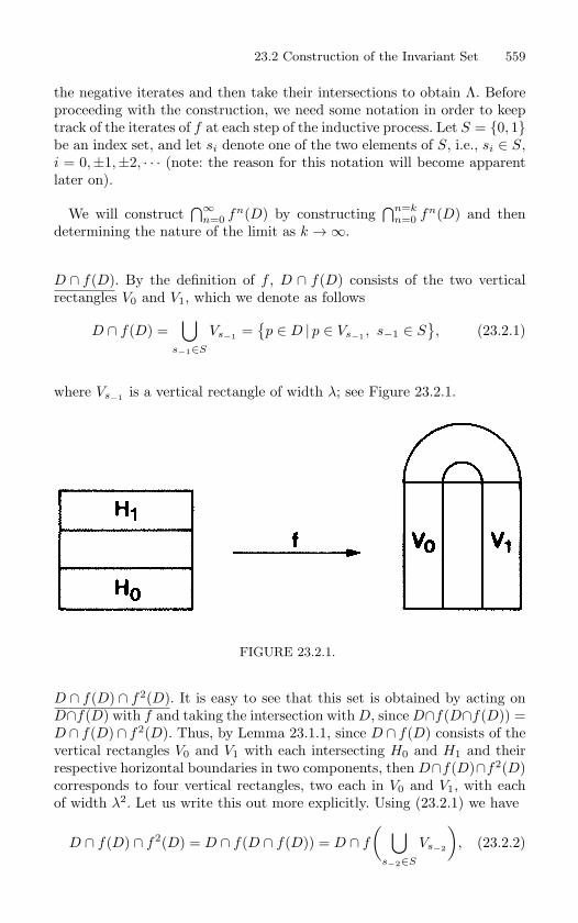
23.2 Construction of the Invariant Set 559
the negative iterates and then take their intersections to obtain Λ. Beforeproceeding with the construction, we need some notation in order to keeptrack of the iterates of f at each step of the inductive process. Let S = 0, 1be an index set, and let si denote one of the two elements of S, i.e., si ∈ S,i = 0,±1,±2, · · · (note: the reason for this notation will become apparentlater on).
We will construct⋂∞
n=0 fn(D) by constructing⋂n=k
n=0 fn(D) and thendetermining the nature of the limit as k →∞.
D ∩ f(D). By the definition of f , D ∩ f(D) consists of the two verticalrectangles V0 and V1, which we denote as follows
D ∩ f(D) =⋃
s−1∈S
Vs−1 =p ∈ D | p ∈ Vs−1 , s−1 ∈ S
, (23.2.1)
where Vs−1 is a vertical rectangle of width λ; see Figure 23.2.1.
FIGURE 23.2.1.
D ∩ f(D) ∩ f2(D). It is easy to see that this set is obtained by acting onD∩f(D) with f and taking the intersection with D, since D∩f(D∩f(D)) =D ∩ f(D)∩ f2(D). Thus, by Lemma 23.1.1, since D ∩ f(D) consists of thevertical rectangles V0 and V1 with each intersecting H0 and H1 and theirrespective horizontal boundaries in two components, then D∩f(D)∩f2(D)corresponds to four vertical rectangles, two each in V0 and V1, with eachof width λ2. Let us write this out more explicitly. Using (23.2.1) we have
D ∩ f(D) ∩ f2(D) = D ∩ f(D ∩ f(D)) = D ∩ f
( ⋃s−2∈S
Vs−2
), (23.2.2)
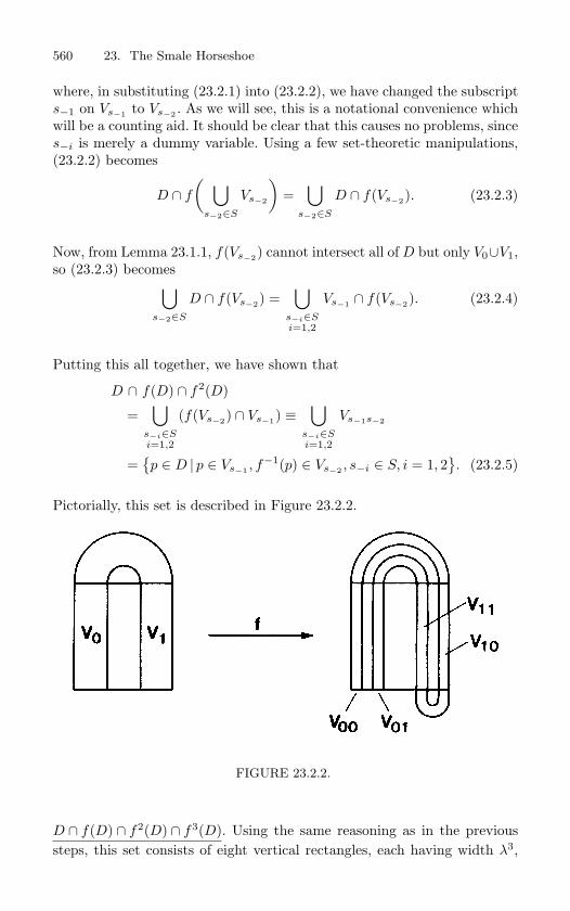
560 23. The Smale Horseshoe
where, in substituting (23.2.1) into (23.2.2), we have changed the subscripts−1 on Vs−1 to Vs−2 . As we will see, this is a notational convenience whichwill be a counting aid. It should be clear that this causes no problems, sinces−i is merely a dummy variable. Using a few set-theoretic manipulations,(23.2.2) becomes
D ∩ f
( ⋃s−2∈S
Vs−2
)=
⋃s−2∈S
D ∩ f(Vs−2). (23.2.3)
Now, from Lemma 23.1.1, f(Vs−2) cannot intersect all of D but only V0∪V1,so (23.2.3) becomes⋃
s−2∈S
D ∩ f(Vs−2) =⋃
s−i∈Si=1,2
Vs−1 ∩ f(Vs−2). (23.2.4)
Putting this all together, we have shown that
D ∩ f(D) ∩ f2(D)
=⋃
s−i∈Si=1,2
(f(Vs−2) ∩ Vs−1) ≡⋃
s−i∈Si=1,2
Vs−1s−2
=p ∈ D | p ∈ Vs−1 , f
−1(p) ∈ Vs−2 , s−i ∈ S, i = 1, 2. (23.2.5)
Pictorially, this set is described in Figure 23.2.2.
FIGURE 23.2.2.
D ∩ f(D) ∩ f2(D) ∩ f3(D). Using the same reasoning as in the previoussteps, this set consists of eight vertical rectangles, each having width λ3,
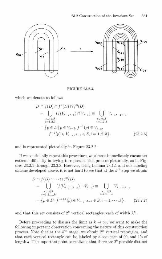
23.2 Construction of the Invariant Set 561
FIGURE 23.2.3.
which we denote as follows
D ∩ f(D) ∩ f2(D) ∩ f3(D)
=⋃
s−1∈Si=1,2,3
(f(Vs−2s−3) ∩ Vs−1) ≡⋃
s−i∈Si=1,2,3
Vs−1s−2s−3
=p ∈ D | p ∈ Vs−1, f
−1(p) ∈ Vs−2 ,
f−2(p) ∈ Vs−3 , s−i ∈ S, i = 1, 2, 3, (23.2.6)
and is represented pictorially in Figure 23.2.2.
If we continually repeat this procedure, we almost immediately encounterextreme difficulty in trying to represent this process pictorially, as in Fig-ures 23.2.1 through 23.2.3. However, using Lemma 23.1.1 and our labelingscheme developed above, it is not hard to see that at the kth step we obtain
D ∩ f(D) ∩ · · · ∩ fk(D)
=⋃
s−i∈Si=1,2,...,k
(f(Vs−2···s−k) ∩ Vs−1) ≡
⋃s−i∈S
i=1,2,...,k
Vs−1···s−k
=p ∈ D | f−i+1(p) ∈ Vs−i
, s−i ∈ S, i = 1, · · · , k
(23.2.7)
and that this set consists of 2k vertical rectangles, each of width λk.
Before proceeding to discuss the limit as k → ∞, we want to make thefollowing important observation concerning the nature of this constructionprocess. Note that at the kth stage, we obtain 2k vertical rectangles, andthat each vertical rectangle can be labeled by a sequence of 0’s and 1’s oflength k. The important point to realize is that there are 2k possible distinct
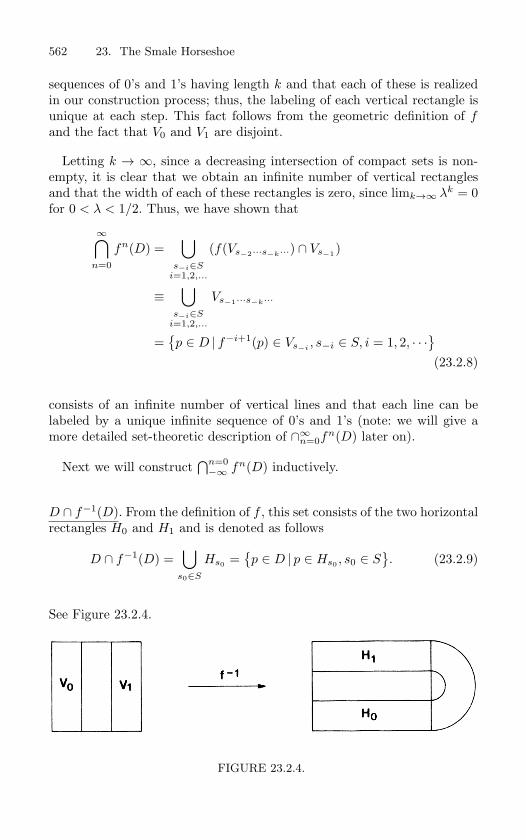
562 23. The Smale Horseshoe
sequences of 0’s and 1’s having length k and that each of these is realizedin our construction process; thus, the labeling of each vertical rectangle isunique at each step. This fact follows from the geometric definition of fand the fact that V0 and V1 are disjoint.
Letting k → ∞, since a decreasing intersection of compact sets is non-empty, it is clear that we obtain an infinite number of vertical rectanglesand that the width of each of these rectangles is zero, since limk→∞ λk = 0for 0 < λ < 1/2. Thus, we have shown that
∞⋂n=0
fn(D) =⋃
s−i∈Si=1,2,...
(f(Vs−2···s−k···) ∩ Vs−1)
≡⋃
s−i∈Si=1,2,...
Vs−1···s−k···
=p ∈ D | f−i+1(p) ∈ Vs−i
, s−i ∈ S, i = 1, 2, · · ·(23.2.8)
consists of an infinite number of vertical lines and that each line can belabeled by a unique infinite sequence of 0’s and 1’s (note: we will give amore detailed set-theoretic description of ∩∞
n=0fn(D) later on).
Next we will construct⋂n=0
−∞ fn(D) inductively.
D ∩ f−1(D). From the definition of f , this set consists of the two horizontalrectangles H0 and H1 and is denoted as follows
D ∩ f−1(D) =⋃
s0∈S
Hs0 =p ∈ D | p ∈ Hs0 , s0 ∈ S
. (23.2.9)
See Figure 23.2.4.
FIGURE 23.2.4.
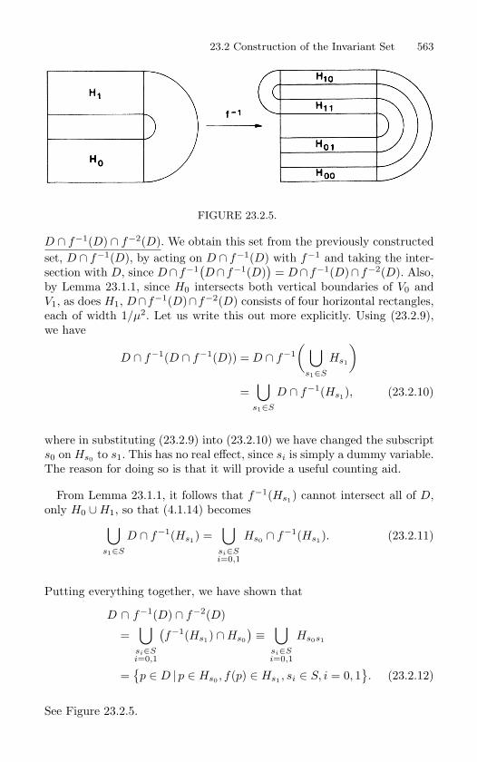
23.2 Construction of the Invariant Set 563
FIGURE 23.2.5.
D ∩ f−1(D) ∩ f−2(D). We obtain this set from the previously constructedset, D ∩ f−1(D), by acting on D ∩ f−1(D) with f−1 and taking the inter-section with D, since D∩f−1
(D∩f−1(D)
)= D∩f−1(D)∩f−2(D). Also,
by Lemma 23.1.1, since H0 intersects both vertical boundaries of V0 andV1, as does H1, D∩f−1(D)∩f−2(D) consists of four horizontal rectangles,each of width 1/µ2. Let us write this out more explicitly. Using (23.2.9),we have
D ∩ f−1(D ∩ f−1(D)) = D ∩ f−1( ⋃
s1∈S
Hs1
)
=⋃
s1∈S
D ∩ f−1(Hs1), (23.2.10)
where in substituting (23.2.9) into (23.2.10) we have changed the subscripts0 on Hs0 to s1. This has no real effect, since si is simply a dummy variable.The reason for doing so is that it will provide a useful counting aid.
From Lemma 23.1.1, it follows that f−1(Hs1) cannot intersect all of D,only H0 ∪H1, so that (4.1.14) becomes⋃
s1∈S
D ∩ f−1(Hs1) =⋃
si∈Si=0,1
Hs0 ∩ f−1(Hs1). (23.2.11)
Putting everything together, we have shown that
D ∩ f−1(D) ∩ f−2(D)
=⋃
si∈Si=0,1
(f−1(Hs1) ∩Hs0
)≡
⋃si∈Si=0,1
Hs0s1
=p ∈ D | p ∈ Hs0 , f(p) ∈ Hs1 , si ∈ S, i = 0, 1
. (23.2.12)
See Figure 23.2.5.
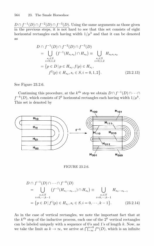
564 23. The Smale Horseshoe
D ∩ f−1(D) ∩ f−2(D) ∩ f−3(D). Using the same arguments as those givenin the previous steps, it is not hard to see that this set consists of eighthorizontal rectangles each having width 1/µ3 and that it can be denotedas
D ∩ f−1(D) ∩ f−2(D) ∩ f−3(D)
=⋃
si∈Si=0,1,2
(f−1(Hs1s2) ∩Hs0
)≡
⋃si∈S
i=0,1,2
Hs0s1s2
=p ∈ D | p ∈ Hs0 , f(p) ∈ Hs1 ,
f2(p) ∈ Hs2 , si ∈ S, i = 0, 1, 2. (23.2.13)
See Figure 23.2.6.
Continuing this procedure, at the kth step we obtain D ∩ f−1(D)∩ · · · ∩f−k(D), which consists of 2k horizontal rectangles each having width 1/µk.This set is denoted by
FIGURE 23.2.6.
D ∩ f−1(D) ∩ · · · ∩ f−k(D)
=⋃
si∈Si=0,···,k−1
(f−1(Hs1···sk−1) ∩Hs0
)≡
⋃si∈S
i=0,···,k−1
Hs0···sk−1
=p ∈ D | f i(p) ∈ Hsi
, si ∈ S, i = 0, · · · , k − 1. (23.2.14)
As in the case of vertical rectangles, we note the important fact that atthe kth step of the inductive process, each one of the 2k vertical rectanglescan be labeled uniquely with a sequence of 0’s and 1’s of length k. Now, aswe take the limit as k →∞, we arrive at
⋂n=0−∞ fn(D), which is an infinite
23.2 Construction of the Invariant Set 565
set of horizontal lines, since a decreasing intersection of compact sets isnonempty and the width of each component of the intersection is givenby limk→∞(1/µk) = 0, µ > 2. Each line is labeled by a unique infinitesequence of 0’s and 1’s as follows
n=0⋂−∞
fn(D) =⋃
si∈Si=0,1,···
(f(Hs1···sk···) ∩Hs0
)≡
⋃si∈S
i=0,1,···
Hs0···sk···
=p ∈ D | f i(p) ∈ Hsi
, si ∈ S, i = 0, 1, · · ·. (23.2.15)
Thus, we have
Λ =∞⋂
n=−∞fn(D) =
[ 0⋂n=−∞
fn(D)]∩[ ∞⋂
n=0
fn(D)], (23.2.16)
which consists of an infinite set of points, since each vertical line in⋂∞n=0 fn(D) intersects each horizontal line in
⋂n=0−∞ fn(D) in a unique
point. Furthermore, each point p ∈ Λ can be labeled uniquely by a bi-infinite sequence of 0’s and 1’s which is obtained by concatenating thesequences associated with the respective vertical and horizontal lines thatserve to define p. Stated more precisely, let s−1 · · · s−k · · · be a particularinfinite sequence of 0’s and 1’s; then Vs−1···s−k··· corresponds to a uniquevertical line. Let s0 · · · sk · · · likewise be a particular infinite sequence of0’s and 1’s; then Hs0···sk··· corresponds to a unique horizontal line. Now ahorizontal line and vertical line intersect in a unique point p; thus, we havea well-defined map from points p ∈ Λ to bi-infinite sequences of 0’s and 1’swhich we call φ.
pφ−→ · · · s−k · · · s−1s0 · · · sk · · · .
Notice that because
Vs−1···s−k··· =p ∈ D | f−i+1(p) ∈ Vs−i
, i = 1, · · ·
=p ∈ D | f−i(p) ∈ Hs−i
, i = 1, · · ·
since f(Hsi) = Vsi
(23.2.17)
andHs0···sk··· =
p ∈ D | f i(p) ∈ Hsi , i = 0, · · ·
, (23.2.18)
we have
p = Vs−1···s−k··· ∩Hs0···sk···
=p ∈ D | f i(p) ∈ Hsi
, i = 0,±1,±2, · · ·. (23.2.19)
566 23. The Smale Horseshoe
Therefore, we see that the unique sequence of 0’s and 1’s we have associatedwith p contains information concerning the behavior of p under iterationby f . In particular, the skth element in the sequence associated with pindicates that fk(p) ∈ Hsk
. Now, note that for the bi-infinite sequence of0’s and 1’s associated with p, the decimal point separates the past iteratesfrom the future iterates; thus, the sequence of 0’s and 1’s associated withfk(p) is obtained from the sequence associated with p merely by shiftingthe decimal point in the sequence associated with p k places to the right ifk is positive or k places to the left if k is negative, until sk is the symbolimmediately to the right of the decimal point. We can define a map ofbi-infinite sequences of 0’s and 1’s, called the shift map, σ, which takes asequence and shifts the decimal point one place to the right. Therefore,if we consider a point p ∈ Λ and its associated bi-infinite sequence of 0’sand 1’s, φ(p), we can take any iterate of p, fk(p), and we can immediatelyobtain its associated bi-infinite sequence of 0’s and 1’s given by σk(φ(p)).Hence, there is a direct relationship between iterating any point p ∈ Λunder f and iterating the sequence of 0’s and 1’s associated with p underthe shift map σ.
Now, at this point, it is not clear where we are going with this analogybetween points in Λ and bi-infinite sequences of 0’s and 1’s since, althoughthe sequence associated with a given point p ∈ Λ contains information onthe entire future and past as to whether or not it is in H0 or H1 for anygiven iterate, it is not hard to imagine different points, both contained inthe same horizontal rectangle after any given iteration, whose orbits arecompletely different. The fact that this cannot happen for our map andthat the dynamics of f on Λ are completely modeled by the dynamics ofthe shift map acting on sequences of 0’s and 1’s is an amazing fact which,to justify, we must digress into symbolic dynamics.
23.3 Symbolic Dynamics
Let S = 0, 1 be the set of nonnegative integers consisting of 0 and 1. LetΣ be the collection of all bi-infinite sequences of elements of S, i.e., s ∈ Σimplies
s =· · · s−n · · · s−1.s0 · · · sn · · ·
, si ∈ S ∀ i.
We will refer to Σ as the space of bi-infinite sequences of two symbols. Wewish to introduce some structure on Σ in the form of a metric, d(·, ·), whichwe do as follows. Consider
s = · · · s−n · · · s−1.s0 · · · sn · · ·,
23.3 Symbolic Dynamics 567
s = · · · s−n · · · s−1.s0 · · · sn · · · ∈ Σ;
we define the distance between s and s, denoted d(s, s), as follows
d(s, s) =∞∑
i=−∞
δi
2|i| where δi =
0 if si = si,1 if si = si.
(23.3.1)
Thus, two sequences are “close” if they agree on a long central block. (Note:the reader should check that d(·, ·) does indeed satisfy the properties of ametric. See Devaney [1986] for a proof.)
We consider a map of Σ into itself, which we shall call the shift map, σ,defined as follows: For s = · · · s−n · · · s−1.s0s1 · · · sn · · · ∈ Σ, we define
σ(s) = · · · s−n · · · s−1s0.s1 · · · sn · · ·
or σ(s)i = si+1. Also, σ is continuous; we give a proof of this later inSection 24. Next, we want to consider the dynamics of σ on Σ (note: forour purposes the phrase “dynamics of σ on Σ” refers to the orbits of pointsin Σ under iteration by σ). It should be clear that σ has precisely twofixed points, namely, the sequence whose elements are all zeros and thesequence whose elements are all ones (notation: bi-infinite sequences whichperiodically repeat after some fixed length will be denoted by the finitelength sequence with an overbar, e.g., · · · 101010.101010 · · · is denotedby 10.10).
In particular, it is easy to see that the orbits of sequences which period-ically repeat are periodic under iteration by σ. For example, consider thesequence 10.10. We have
σ10.10 = 01.01,
andσ01.10 = 10.10;
thus,σ210.10 = 10.10.
Therefore, the orbit of 10.10 is an orbit of period two for σ. So, fromthis particular example, it is easy to see that for any fixed k, the orbitsof σ having period k correspond to the orbits of sequences made up ofperiodically repeating blocks of 0’s and 1’s with the blocks having length
568 23. The Smale Horseshoe
k. Thus, since for any fixed k the number of sequences having a periodicallyrepeating block of length k is finite, we see that σ has a countable infinityof periodic orbits having all possible periods. We list the first few below.
Period 1 : 0.0, 1.1Period 2 : 01.01 σ−→ 10.10 σ−→ 01.01Period 3 : 001.001 σ−→ 010.010 σ−→ 100.100 σ−→ 001.001
: 110.110 σ−→ 101.101 σ−→ 011.011 σ−→ 110.110...
etc.
Also, σ has an uncountable number of nonperiodic orbits. To show this,we need only construct a nonperiodic sequence and show that there are anuncountable number of such sequences. A proof of this fact goes as follows:we can easily associate an infinite sequence of 0’s and 1’s with a givenbi-infinite sequence by the following rule
· · · s−n · · · s−1.s0 · · · sn · · · → .s0s1s−1s2s−2 · · · .
Now, we will take it as a known fact that the irrational numbers in theclosed unit interval [0, 1] constitute an uncountable set, and that everynumber in this interval can be expressed in base 2 as a binary expansionof 0’s and 1’s with the irrational numbers corresponding to nonrepeatingsequences. Thus, we have a one-to-one correspondence between an uncount-able set of points and nonrepeating sequences of 1’s and 0’s. As a result,the orbits of these sequences are the nonperiodic orbits of σ, and there arean uncountable number of such orbits.
Another interesting fact concerning the dynamics of σ on Σ is that thereexists an element, say s ∈ Σ, whose orbit is dense in Σ, i.e., for any givens′ ∈ Σ and ε > 0, there exists some integer n such that d(σn(s), s′) <ε. This is easiest to see by constructing s directly. We do this by firstconstructing all possible sequences of 0’s and 1’s having length 1, 2, 3, . . . .This process is well defined in a set-theoretic sense, since there are onlya finite number of possibilities at each step (more specifically, there are2k distinct sequences of 0’s and 1’s of length k). The first few of thesesequences would be as follows
length 1 : 0, 1length 2 : 00, 01, 10, 11length 3 : 000, 001, 010, 011, 100, 101, 110, 111
......etc.
23.3 Symbolic Dynamics 569
We can now introduce an ordering on the collection of sequences of 0’s and1’s in order to keep track of the different sequences in the following way.Consider two finite sequences of 0’s and 1’s
s = s1 · · · sk, s = s1 · · · sk′.
We can then says < s if k < k′.
If k = k′, thens < s if si < si,
where i is the first integer such that si = si. For example, using thisordering we have
0 < 1,0 < 00,00 < 01, etc.
This ordering gives us a systematic way of distinguishing different sequencesthat have the same length. Thus, we will denote the sequences of 0’s and1’s having length k as follows
sk1 < · · · < sk
2k ,
where the superscript refers to the length of the sequence and the subscriptrefers to a particular sequence of length k which is uniquely specified bythe above ordering scheme. This will give us a systematic way of writingdown our candidate for a dense orbit.
Now consider the following sequence
s = · · · s38s
36s
34s
32s
24s
22s
12.s
11s
21s
23s
31s
33s
35s
37 · · ·.
Thus, s contains all possible sequences of 0’s and 1’s of any fixed length.To show that the orbit of s is dense in Σ, we argue as follows: let s′ bean arbitrary point in Σ and let ε > 0 be given. An ε-neighborhood of s′
consists of all points s′′ ∈ Σ such that d(s′, s′′) < ε, where d is the metricgiven in (23.3.1). Therefore, by definition of the metric on Σ, there mustbe some integer N = N(ε) such that s′
i = s′′i , |i| ≤ N (note: a proof of this
statement can be found in Devaney [1986] or in Chapter 24). By construc-tion, the finite sequence s′
−N · · · s′−1.s
′0 · · · s′
N is contained somewhere in
570 23. The Smale Horseshoe
s; therefore, there must be some integer N such that d(σN (s), s′) < ε, and
we can then conclude that the orbit of s is dense in Σ.
We summarize these facts concerning the dynamics of σ on Σ in thefollowing theorem.
Theorem 23.3.1 The shift map σ acting on the space of bi-infinite se-
quences of 0’s and 1’s, Σ, has
i) a countable infinity of periodic orbits of arbitrarily high period;
ii) an uncountable infinity of nonperiodic orbits;
iii) a dense orbit.
23.4 The Dynamics on the Invariant Set
At this point we want to relate the dynamics of σ on Σ, about which we havea great deal of information, to the dynamics of the Smale horseshoe f onits invariant set Λ, about which we know little except for its complicatedgeometric structure. Recall that we have shown the existence of a well-defined map φ which associates to each point, p ∈ Λ, a bi-infinite sequenceof 0’s and 1’s, φ(p). Furthermore, we noted that the sequence associatedwith any iterate of p, say fk(p), can be found merely by shifting the decimalpoint in the sequence associated with p k places to the right if k is positiveor k places to the left if k is negative. In particular, the relation σ φ(p) =φ f(p) holds for every p ∈ Λ. Now, if φ were invertible and continuous(continuity is necessary since f is continuous), the following relationshipwould hold
φ−1 σ φ(p) = f(p) ∀ p ∈ Λ. (23.4.1)
Thus, if the orbit p ∈ Λ under f is denoted by· · · f−n(p), · · · , f−1(p), p, f(p), · · · , fn(p), · · ·
, (23.4.2)
then, since φ−1 σ φ(p) = f(p), we see that
fn(p) =(φ−1 σ φ
)(φ−1 σ φ
) · · ·
(φ−1 σ φ(p)
)= φ−1 σn φ(p), n ≥ 0. (23.4.3)
Also, from (23.4.1) we have
23.4 The Dynamics on the Invariant Set 571
f−1(p) = φ−1 σ−1 φ(p) ∀ p ∈ Λ,
from which we see that
f−n(p) =(φ−1 σ−1 φ
)(φ−1 σ−1 φ)
) · · ·
(φ−1 σ−1 φ(p)
)= φ−1 σ−n φ(p), n ≥ 0. (23.4.4)
Therefore, using (23.4.2), (23.4.3), and (23.4.4), we see that the orbit ofp ∈ Λ under f would correspond directly to the orbit of φ(p) under σ inΣ. In particular, the entire orbit structure of σ on Σ would be identical tothe structure of f on Λ. Hence, in order to verify that this situation holds,we need to show that φ is a homeomorphism of Λ and Σ.
Theorem 23.4.1 The map φ : Λ → Σ is a homeomorphism.
Proof: We need only show that φ is one-to-one and continuous, since con-tinuity of the inverse will follow from the fact that one-to-one, onto, andcontinuous maps from compact sets into Hausdorff spaces are homeomor-phisms (see Dugundji [1966]). We prove each condition separately.
φ is one-to-one: This means that given p, p′ ∈ Λ, if p = p′, then φ(p) =φ(p′).
We give a proof by contradiction. Suppose p = p′ and
φ(p) = φ(p′) =· · · s−n · · · s−1.s0 · · · sn · · ·
.
Then, by construction of Λ, p and p′ lie in the intersection of the verticalline Vs−1···s−n··· and the horizontal line Hs0···sn···. However, the intersectionof a horizontal line and a vertical line consists of a unique point; thereforep = p′, contradicting our original assumption. This contradiction is due tothe fact that we have assumed φ(p) = φ(p′); thus, for p = p′, φ(p) = φ(p′).
φ is onto: This means that given any bi-infinite sequence of 0’s and 1’sin Σ, say · · · s−n · · · s−1.s0 · · · sn · · ·, there is a point p ∈ Λ such thatφ(p) = · · · s−n · · · s−1.s0 · · · sn · · ·.
The proof goes as follows: Recall the construction of⋂∞
n=0 fn(D) and⋂n=0−∞ fn(D); given any infinite sequence of 0’s and 1’s, · · · s−n · · · s−1.,
there is a unique vertical line in⋂∞
n=0 fn(D) corresponding to thissequence. Similarly, given any infinite sequence of 0’s and 1’s, .s0
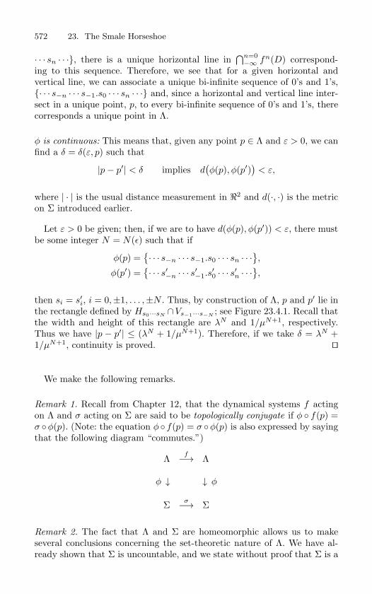
572 23. The Smale Horseshoe
· · · sn · · ·, there is a unique horizontal line in⋂n=0
−∞ fn(D) correspond-ing to this sequence. Therefore, we see that for a given horizontal andvertical line, we can associate a unique bi-infinite sequence of 0’s and 1’s,· · · s−n · · · s−1.s0 · · · sn · · · and, since a horizontal and vertical line inter-sect in a unique point, p, to every bi-infinite sequence of 0’s and 1’s, therecorresponds a unique point in Λ.
φ is continuous: This means that, given any point p ∈ Λ and ε > 0, we canfind a δ = δ(ε, p) such that
|p− p′| < δ implies d(φ(p), φ(p′)
)< ε,
where | · | is the usual distance measurement in 2 and d(·, ·) is the metricon Σ introduced earlier.
Let ε > 0 be given; then, if we are to have d(φ(p), φ(p′)) < ε, there mustbe some integer N = N(ε) such that if
φ(p) =· · · s−n · · · s−1.s0 · · · sn · · ·
,
φ(p′) =· · · s′
−n · · · s′−1.s
′0 · · · s′
n · · ·,
then si = s′i, i = 0,±1, . . . ,±N . Thus, by construction of Λ, p and p′ lie in
the rectangle defined by Hs0···sN∩Vs−1···s−N
; see Figure 23.4.1. Recall thatthe width and height of this rectangle are λN and 1/µN+1, respectively.Thus we have |p − p′| ≤ (λN + 1/µN+1). Therefore, if we take δ = λN +1/µN+1, continuity is proved.
We make the following remarks.
Remark 1. Recall from Chapter 12, that the dynamical systems f actingon Λ and σ acting on Σ are said to be topologically conjugate if φ f(p) =σ φ(p). (Note: the equation φ f(p) = σ φ(p) is also expressed by sayingthat the following diagram “commutes.”)
Λf−→ Λ
φ ↓ ↓ φ
Σ σ−→ Σ
Remark 2. The fact that Λ and Σ are homeomorphic allows us to makeseveral conclusions concerning the set-theoretic nature of Λ. We have al-ready shown that Σ is uncountable, and we state without proof that Σ is a
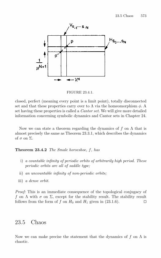
23.5 Chaos 573
FIGURE 23.4.1.
closed, perfect (meaning every point is a limit point), totally disconnectedset and that these properties carry over to Λ via the homeomorphism φ. Aset having these properties is called a Cantor set. We will give more detailedinformation concerning symbolic dynamics and Cantor sets in Chapter 24.
Now we can state a theorem regarding the dynamics of f on Λ that isalmost precisely the same as Theorem 23.3.1, which describes the dynamicsof σ on Σ.
Theorem 23.4.2 The Smale horseshoe, f , has
i) a countable infinity of periodic orbits of arbitrarily high period. These
periodic orbits are all of saddle type;
ii) an uncountable infinity of non-periodic orbits;
iii) a dense orbit.
Proof: This is an immediate consequence of the topological conjugacy off on Λ with σ on Σ, except for the stability result. The stability resultfollows from the form of f on H0 and H1 given in (23.1.6).
23.5 Chaos
Now we can make precise the statement that the dynamics of f on Λ ischaotic.
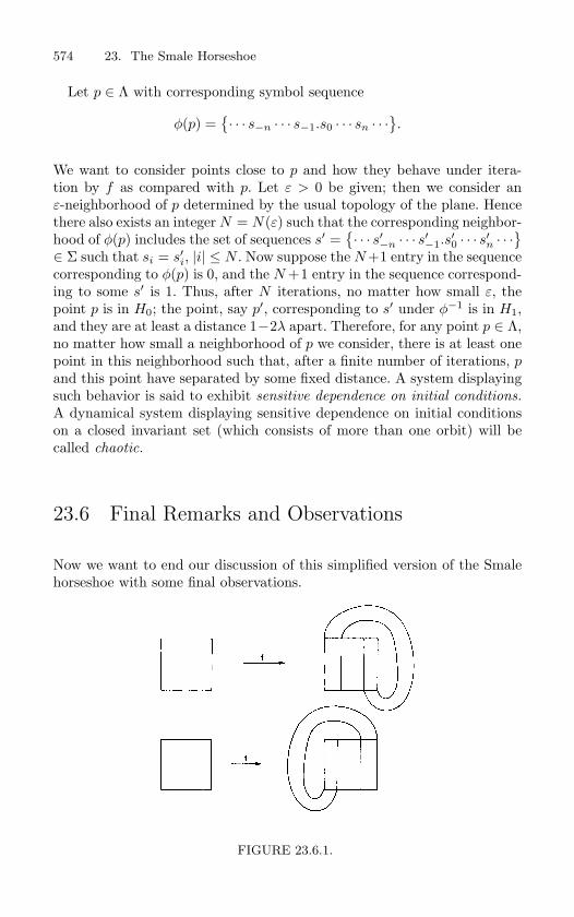
574 23. The Smale Horseshoe
Let p ∈ Λ with corresponding symbol sequence
φ(p) =· · · s−n · · · s−1.s0 · · · sn · · ·
.
We want to consider points close to p and how they behave under itera-tion by f as compared with p. Let ε > 0 be given; then we consider anε-neighborhood of p determined by the usual topology of the plane. Hencethere also exists an integer N = N(ε) such that the corresponding neighbor-hood of φ(p) includes the set of sequences s′ =
· · · s′
−n · · · s′−1.s
′0 · · · s′
n · · ·
∈ Σ such that si = s′i, |i| ≤ N . Now suppose the N+1 entry in the sequence
corresponding to φ(p) is 0, and the N +1 entry in the sequence correspond-ing to some s′ is 1. Thus, after N iterations, no matter how small ε, thepoint p is in H0; the point, say p′, corresponding to s′ under φ−1 is in H1,and they are at least a distance 1−2λ apart. Therefore, for any point p ∈ Λ,no matter how small a neighborhood of p we consider, there is at least onepoint in this neighborhood such that, after a finite number of iterations, pand this point have separated by some fixed distance. A system displayingsuch behavior is said to exhibit sensitive dependence on initial conditions.
A dynamical system displaying sensitive dependence on initial conditionson a closed invariant set (which consists of more than one orbit) will becalled chaotic.
23.6 Final Remarks and Observations
Now we want to end our discussion of this simplified version of the Smalehorseshoe with some final observations.
FIGURE 23.6.1.
23.6 Final Remarks and Observations 575
1. If you consider carefully the main ingredients of f which led to The-orem 23.4.2, you will see that there are two key elements.
(a) The square is contracted, expanded, and folded in such a waythat we can find disjoint regions that are mapped over them-selves.
(b) There exists “strong” stretching and contraction in complemen-tary directions.
2. From observation 1), the fact that the image of the square appears inthe shape of a horseshoe is not important. Other possible scenariosare shown in Figure 23.6.1.
3. Notice that, in our study of the invariant set of f , we do not considerthe question of the geometry of the points which escape from thesquare. We remark that this could be an interesting research topic,since this more global question may enable one to determine condi-tions under which the horseshoe becomes an attractor.
4. Some interesting references related to the Smale horseshoe are Bowen[1975b], Young [1981], Hall [1994] and Kennedy and Yorke[ 2001].
24
Symbolic Dynamics
In the previous section we saw an example of a two-dimensional map whichpossessed an invariant Cantor set. The map, restricted to its invariant set,was shown to have a countable infinity of periodic orbits of all periods, anuncountable infinity of nonperiodic orbits, and a dense orbit. Now, in gen-eral, the determination of such detailed information concerning the orbitstructure of a map is not possible. However, in our example we were able toshow that the map restricted to its invariant set behaved the same as theshift map acting on the space of bi-infinite sequences of 0’s and 1’s (moreprecisely, these two dynamical systems were shown to be topologically con-jugate; thus their orbit structures are identical). The shift map was no lesscomplicated than our original map but, due to its structure, many of thefeatures concerning its dynamics (e.g., the nature and number of its peri-odic orbits) were more or less obvious. The technique of characterizing theorbit structure of a dynamical system via infinite sequences of “symbols”(in our case 0’s and 1’s) is known as symbolic dynamics. The technique isnot new and appears to have originally been applied by Hadamard [1898]in the study of geodesics on surfaces of negative curvature and Birkhoff[1927], [1935] in his studies of dynamical systems. The first exposition ofsymbolic dynamics as an independent subject was given by Morse and Hed-lund [1938]. Applications of this idea to differential equations can be foundin Levinson’s work on the forced van der Pol equation (Levinson [1949]),from which came Smale’s inspiration for his construction of the horseshoemap (Smale [1963], [1980]), and also in the work of Alekseev [1968], [1969],who gives a systematic account of the technique and applies it to problemsarising from celestial mechanics. These references by no means represent acomplete account of the history of symbolic dynamics or of its applications,and we refer the reader to the bibliographies of the above listed referencesor to Moser [1973] or Lind and Marcus [1995] for a more complete list ofreferences on the subject and its applications. In recent times (say fromabout 1965 to the present) there has been a flood of applications of thetechnique.
Symbolic dynamics will play a key role in explaining the dynamical phe-nomena we encounter in this chapter. For this reason, we now want to
24.1 The Structure of the Space of Symbol Sequences 577
describe some aspects of symbolic dynamics viewed as an independent sub-ject. Our discussion follows Wiggins [1988].
We let S = 1, 2, 3, · · · , N, N ≥ 2 be our collection of symbols. Wewill build our sequences from elements of S. Note that for the purpose ofconstructing sequences, the elements of S could be anything, e.g., lettersof the alphabet, Chinese characters, etc. We will use positive integers sincethey are familiar, easy to write down, and we have as many of them as wedesire.
24.1 The Structure of the Space of SymbolSequences
We now want to construct the space of all symbol sequences, which wewill refer to as ΣN , from elements of S and derive some properties of ΣN .It will be convenient to construct ΣN as a Cartesian product of infinitelymany copies of S. This construction will allow us to make some conclusionsconcerning the properties of ΣN based only on our knowledge of S, thestructure which we give to S, and topological theorems on infinite products.
We now give some structure to S; specifically, we want to make S into ametric space, which can be done with the following metric
d(a, b) ≡
1 if a = b,
0 if a = b.(24.1.1)
It is trivial to check that d(·, ·) is a metric.
The metric (24.1.1) actually induces the discrete topology on S, i.e.,
the topology defined by the collection of all subsets of S, see Munkres
[1975].
Since S consists of a finite number of points, it is trivial to verify that it iscompact. Moreover, S is totally disconnected, i.e., its only connected sub-sets are one-point sets. We summarize the properties of S in the followingproposition.
Proposition 24.1.1 The set S equipped with the metric (24.1.1) is a com-
pact, totally disconnected, metric space.
578 24. Symbolic Dynamics
We remark that compact metric spaces are automatically complete met-ric spaces (see Munkres [1975], Section 7-3, Theorem 3.1).
Now we will construct ΣN as a bi-infinite Cartesian product of copies ofS:
ΣN ≡ · · ·×S×S×S×S× · · · ≡∞∏
i=−∞Si where Si = S ∀ i. (24.1.2)
Thus, a point in ΣN is represented as a “bi-infinity-tuple” of elements ofS:
s ∈ ΣN ⇒ s =· · · , s−n, · · · , s−1, s0, s1, · · · , sn, · · ·
where si ∈ S ∀ i,
or, more succintly, we will write s as
s =· · · s−n · · · s−1.s0s1 · · · sn · · ·
where si ∈ S ∀ i.
A word should be said about the “decimal point” that appears in eachsymbol sequence and has the effect of separating the symbol sequence intotwo parts, with both parts being infinite (hence the reason for the phrase“bi-infinite sequence”). At present it does not play a major role in ourdiscussion and could easily be left out with all of our results describing thestructure of ΣN going through just the same. In some sense, it serves as astarting point for constructing the sequences by giving us a natural way ofsubscripting each element of a sequence. This notation will prove convenientshortly when we define a metric on ΣN . However, the real significance ofthe decimal point will become apparent when we define and discuss theshift map acting on ΣN and its orbit structure.
In order to discuss limit processes in ΣN , it will be convenient to define ametric on ΣN . Since S is a metric space, it is also possible to define a metricon ΣN . There are many possible choices for a metric on ΣN ; however, wewill utilize the following. For
s =· · · s−n · · · s−1.s0s1 · · · sn · · ·
,
s =· · · s−n · · · s−1.s0s1 · · · sn · · ·
∈ ΣN ,
the distance between s and s is defined as
d(s, s) =∞∑
i=−∞
12|i|
di(si, si)1 + di(si, si)
, (24.1.3)
24.1 The Structure of the Space of Symbol Sequences 579
where di(·, ·) is the metric on Si ≡ S defined in (24.1.1). The reader shouldverify that (24.1.3) indeed defines a metric. Intuitively, this choice of metricimplies that two symbol sequences are “close” if they agree on a long centralblock. The following lemma makes this precise.
Lemma 24.1.2 For s, s ∈ ΣN ,
i) Suppose d(s, s) < 1/(2M+1); then si = si for all |i| ≤ M .
ii) Suppose si = si for |i| ≤ M ; then d(s, s) ≤ 1/(2M ).
Proof: The proof of i) is by contradiction. Suppose the hypothesis of i)holds and there exists some j with |j| ≤ M such that sj = sj . Then thereexists a term in the sum defining d(s, s) of the form
12|j|
dj(sj , sj)1 + dj(sj , sj)
.
However, since sj = sj ,
dj(sj , sj)1 + dj(sj , sj)
=12,
and each term in the sum defining d(s, s) is positive so that we have
d(s, s) ≥ 12|j|
dj(sj , sj)1 + dj(sj , sj)
=1
2|j|+1 ≥1
2M+1 ,
but this contradicts the hypothesis of i).
We now prove ii). If si = si for |i| ≤ M , we have
d(s, s) =i=−(M+1)∑
−∞
12|i|
di(si, si)1 + di(si, si)
+∞∑
i=M+1
12|i|
di(si, si)1 + di(si, si)
;
however,(di(si, si)/(1 + di(si, si))
)= 1/2, so we obtain
d(s, s) ≤ 2∞∑
i=M+1
12i+1 =
12M
.
Armed with our metric, we can define neighborhoods of points in ΣN
and describe limit processes. Suppose we are given a point
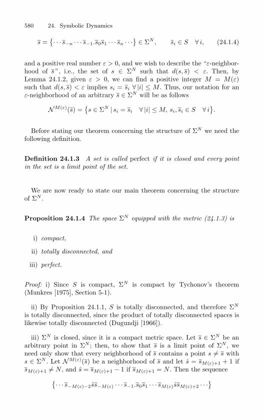
580 24. Symbolic Dynamics
s =· · · s−n · · · s−1.s0s1 · · · sn · · ·
∈ ΣN , si ∈ S ∀ i, (24.1.4)
and a positive real number ε > 0, and we wish to describe the “ε-neighbor-hood of s ”, i.e., the set of s ∈ ΣN such that d(s, s) < ε. Then, byLemma 24.1.2, given ε > 0, we can find a positive integer M = M(ε)such that d(s, s) < ε implies si = si ∀ |i| ≤ M . Thus, our notation for anε-neighborhood of an arbitrary s ∈ ΣN will be as follows
NM(ε)(s) =s ∈ ΣN | si = si ∀ |i| ≤ M, si, si ∈ S ∀ i
.
Before stating our theorem concerning the structure of ΣN we need thefollowing definition.
Definition 24.1.3 A set is called perfect if it is closed and every point
in the set is a limit point of the set.
We are now ready to state our main theorem concerning the structureof ΣN .
Proposition 24.1.4 The space ΣN equipped with the metric (24.1.3) is
i) compact,
ii) totally disconnected, and
iii) perfect.
Proof: i) Since S is compact, ΣN is compact by Tychonov’s theorem(Munkres [1975], Section 5-1).
ii) By Proposition 24.1.1, S is totally disconnected, and therefore ΣN
is totally disconnected, since the product of totally disconnected spaces islikewise totally disconnected (Dugundji [1966]).
iii) ΣN is closed, since it is a compact metric space. Let s ∈ ΣN be anarbitrary point in ΣN ; then, to show that s is a limit point of ΣN , weneed only show that every neighborhood of s contains a point s = s withs ∈ ΣN . Let NM(ε)(s) be a neighborhood of s and let s = sM(ε)+1 + 1 ifsM(ε)+1 = N , and s = sM(ε)+1 − 1 if sM(ε)+1 = N . Then the sequence
· · · s−M(ε)−2ss−M(ε) · · · s−1.s0s1 · · · sM(ε)ssM(ε)+2 · · ·
24.2 The Shift Map 581
is contained in NM(ε)(s) and is not equal to s; thus ΣN is perfect.
We remark that the three properties of ΣN stated in Proposition 24.1.4are often taken as the defining properties of a Cantor set , of which theclassical Cantor “middle-thirds” set is a prime example.
The following theorem of Cantor gives us information concerning thecardinality of perfect sets.
Theorem 24.1.5 Every perfect set in a complete space has at least the
cardinality of the continuum.
Proof: See Hausdorff [1957].
Hence, ΣN is uncountable.
24.2 The Shift Map
Now that we have established the structure of ΣN , we define a map on ΣN ,denoted by σ, as follows. For s = · · · s−n · · · s−1.s0s1 · · · sn · · · ∈ ΣN , wedefine
σ(s) = · · · s−n · · · s−1s0.s1 · · · sn · · ·,
or [σ(s)]i ≡ si+1. The map σ is referred to as the shift map, and when thedomain of σ is taken to be all of ΣN , it is often referred to as a full shift on
N symbols. We have the following proposition concerning some propertiesof σ.
Proposition 24.2.1 i) σ(ΣN ) = ΣN . ii) σ is continuous.
Proof: The proof of i) is obvious. To prove ii) we must show that, givenε > 0, there exists a δ(ε) such that d(s, s) < δ implies d(σ(s), σ(s)) < ε fors, s ∈ ΣN . Suppose ε > 0 is given; then choose M such that 1/(2M−1) < ε.If we then let δ = 1/2M+1, we see by Lemma 24.1.2 that d(s, s) < δ impliessi = si for |i| ≤ M ; hence, [σ(s)]i = [σ(s)]i, |i| ≤ M − 1. Then, also byLemma 24.1.2, we have d(σ(s), σ(s)) < 1/2M−1 < ε.
We now want to consider the orbit structure of σ acting on ΣN . We havethe following proposition.
582 24. Symbolic Dynamics
Proposition 24.2.2 The shift map σ has
i) a countable infinity of periodic orbits consisting of orbits of all periods;
ii) an uncountable infinity of nonperiodic orbits; and
iii) a dense orbit.
Proof: i) This is proven in exactly the same way as the analogous resultobtained in our discussion of the symbolic dynamics for the Smale horse-shoe map in Section 23.3. In particular, the orbits of the periodic symbolsequences are periodic, and there is a countable infinity of such sequences.ii) By Theorem 24.1.5 ΣN is uncountable; thus, removing the countableinfinity of periodic symbol sequences leaves an uncountable number of non-periodic symbol sequences. Since the orbits of the nonperiodic sequencesnever repeat, this proves ii). iii) This is proven in exactly the same way asthe analogous result obtained in our discussion of the Smale horseshoe mapin Section 23; namely, we form a symbol sequence by stringing together allpossible symbol sequences of any finite length. The orbit of this sequenceis dense in ΣN since, by construction, some iterate of this symbol sequencewill be arbitrarily close to any given symbol sequence in ΣN .
24.3 Exercises
1. Compute the distinct period k orbits, k = 1, 2, 3, 4, 5, for σ : ΣN → ΣN , N = 2, 3, 4, 5.
2. Prove that σ : ΣN → ΣN has an infinite number of dense orbits. Are these denseorbits countable?
3. Consider a sequence s ∈ ΣN . Let O(s) denote the orbit of s under the shift map σ.Then the orbit of a sequence s ∈ ΣN is said to be homoclinic to O(s) if
lim|n|→∞
d(σn(s), O(s)) = 0.
(a) Prove that any periodic sequence s has a countable number of homoclinic orbits.
(b) Is this true for nonperiodic sequences s?
(c) Can a periodic sequence have an infinite number of homoclinic orbits?
4. Consider two sequences s, s ∈ ΣN . Then the orbit of any point s ∈ ΣN is said to beheteroclinic to O(s) and O(s) if
limn→∞ d(σn(s), O(s)) = 0 and lim
n→−∞d(σn(s), O(s)) = 0.
(a) Prove that any periodic sequences s, s ∈ ΣN , have a countable number ofheteroclinic orbits.
(b) Is this true for nonperiodic sequences?
(c) Can two periodic sequences have an infinite number of heteroclinic orbits?
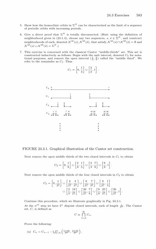
24.3 Exercises 583
5. Show how the homoclinic orbits in ΣN can be characterized as the limit of a sequenceof periodic orbits with increasing periods.
6. Give a direct proof that ΣN is totally disconnected. (Hint: using the definition ofneighborhood given in (24.1.4), choose any two sequences, s, s ∈ ΣN , and constructneighborhoods of each, denoted N M (s), N M (s), that satisfy N M (s)∩N M (s) = ∅ andN M (s) ∪ N M (s) = ΣN .)
7. This exercise is concerned with the classical Cantor “middle-thirds” set. This set isconstructed inductively as follows: Begin with the unit interval, denoted C0 for nota-tional purposes, and remove the open interval ( 1
3 , 23 ) called the “middle third”. We
refer to the remainder as C1. Thus
C1 =[0,
13
]∪[
23
, 1]
.
0 1
3_
3_1 2
9_2_19
_9
_9
7 8
27_
27_
27_
1 2 7 827_
27_19 20
27_
27_
27_
25 26
0
1
2
3
C
C
C
C
FIGURE 24.3.1. Graphical illustration of the Cantor set construction.
Next remove the open middle thirds of the two closed intervals in C1 to obtain
C2 =[0,
19
]∪[
29
,13
]∪[
23
,79
]∪[
89
, 1]
.
Next remove the open middle thirds of the four closed intervals in C2 to obtain
C3 =[0,
127
]∪[
227
,327
]∪[
627
,727
]∪[
827
,13
]
∪[
23
,1927
]∪[
2027
,79
]∪[
89
,2527
]∪[
2627
, 1]
.
Continue this procedure, which we illustrate graphically in Fig. 24.3.1.
At the nth step we have 2n disjoint closed intervals, each of length 13n . The Cantor
set, C, is defined as
C ≡∞⋂
n=0
Cn.
Prove the following:
(a) Cn = Cn−1 −⋃∞
k=0
(1+3k3n , 2+3k
3n
).
584 24. Symbolic Dynamics
(b) C is compact.
(c) C is closed.
(d) C is uncountable.
(e) C is perfect.
(f) C is totally disconnected.
(g) C has Lebesgue measure zero.
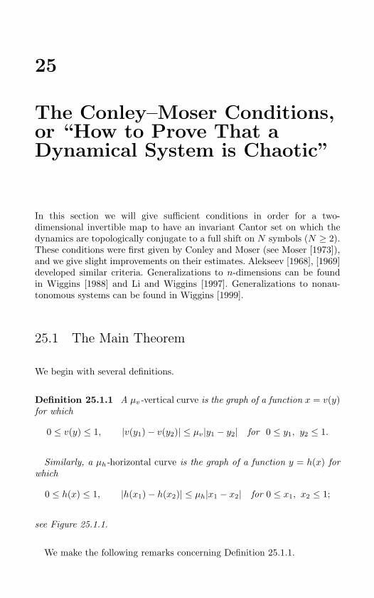
25
The Conley–Moser Conditions,or “How to Prove That aDynamical System is Chaotic”
In this section we will give sufficient conditions in order for a two-dimensional invertible map to have an invariant Cantor set on which thedynamics are topologically conjugate to a full shift on N symbols (N ≥ 2).These conditions were first given by Conley and Moser (see Moser [1973]),and we give slight improvements on their estimates. Alekseev [1968], [1969]developed similar criteria. Generalizations to n-dimensions can be foundin Wiggins [1988] and Li and Wiggins [1997]. Generalizations to nonau-tonomous systems can be found in Wiggins [1999].
25.1 The Main Theorem
We begin with several definitions.
Definition 25.1.1 A µv-vertical curve is the graph of a function x = v(y)for which
0 ≤ v(y) ≤ 1, |v(y1)− v(y2)| ≤ µv|y1 − y2| for 0 ≤ y1, y2 ≤ 1.
Similarly, a µh-horizontal curve is the graph of a function y = h(x) for
which
0 ≤ h(x) ≤ 1, |h(x1)− h(x2)| ≤ µh|x1 − x2| for 0 ≤ x1, x2 ≤ 1;
see Figure 25.1.1.
We make the following remarks concerning Definition 25.1.1.
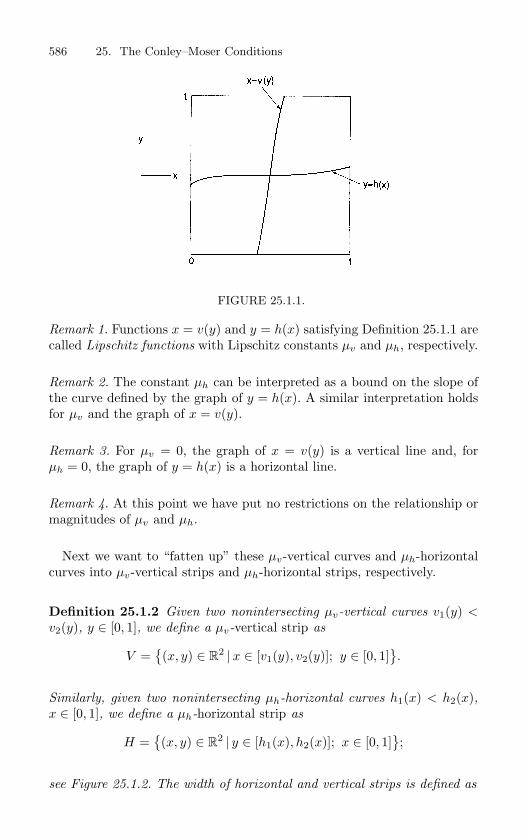
586 25. The Conley–Moser Conditions
FIGURE 25.1.1.
Remark 1. Functions x = v(y) and y = h(x) satisfying Definition 25.1.1 arecalled Lipschitz functions with Lipschitz constants µv and µh, respectively.
Remark 2. The constant µh can be interpreted as a bound on the slope ofthe curve defined by the graph of y = h(x). A similar interpretation holdsfor µv and the graph of x = v(y).
Remark 3. For µv = 0, the graph of x = v(y) is a vertical line and, forµh = 0, the graph of y = h(x) is a horizontal line.
Remark 4. At this point we have put no restrictions on the relationship ormagnitudes of µv and µh.
Next we want to “fatten up” these µv-vertical curves and µh-horizontalcurves into µv-vertical strips and µh-horizontal strips, respectively.
Definition 25.1.2 Given two nonintersecting µv-vertical curves v1(y) <v2(y), y ∈ [0, 1], we define a µv-vertical strip as
V =(x, y) ∈ R
2 |x ∈ [v1(y), v2(y)]; y ∈ [0, 1].
Similarly, given two nonintersecting µh-horizontal curves h1(x) < h2(x),x ∈ [0, 1], we define a µh-horizontal strip as
H =(x, y) ∈ R
2 | y ∈ [h1(x), h2(x)]; x ∈ [0, 1];
see Figure 25.1.2. The width of horizontal and vertical strips is defined as
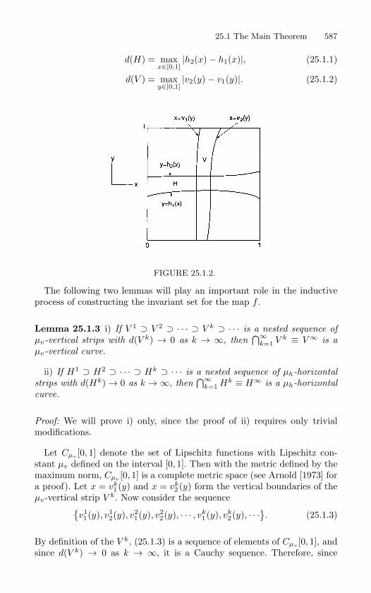
25.1 The Main Theorem 587
d(H) = maxx∈[0,1]
|h2(x)− h1(x)|, (25.1.1)
d(V ) = maxy∈[0,1]
|v2(y)− v1(y)|. (25.1.2)
FIGURE 25.1.2.
The following two lemmas will play an important role in the inductiveprocess of constructing the invariant set for the map f .
Lemma 25.1.3 i) If V 1 ⊃ V 2 ⊃ · · · ⊃ V k ⊃ · · · is a nested sequence of
µv-vertical strips with d(V k) → 0 as k → ∞, then⋂∞
k=1 V k ≡ V ∞ is a
µv-vertical curve.
ii) If H1 ⊃ H2 ⊃ · · · ⊃ Hk ⊃ · · · is a nested sequence of µh-horizontal
strips with d(Hk) → 0 as k →∞, then⋂∞
k=1 Hk ≡ H∞ is a µh-horizontal
curve.
Proof: We will prove i) only, since the proof of ii) requires only trivialmodifications.
Let Cµv[0, 1] denote the set of Lipschitz functions with Lipschitz con-
stant µv defined on the interval [0, 1]. Then with the metric defined by themaximum norm, Cµv [0, 1] is a complete metric space (see Arnold [1973] fora proof). Let x = vk
1 (y) and x = vk2 (y) form the vertical boundaries of the
µv-vertical strip V k. Now consider the sequencev11(y), v1
2(y), v21(y), v2
2(y), · · · , vk1 (y), vk
2 (y), · · ·. (25.1.3)
By definition of the V k, (25.1.3) is a sequence of elements of Cµv[0, 1], and
since d(V k) → 0 as k → ∞, it is a Cauchy sequence. Therefore, since
588 25. The Conley–Moser Conditions
Cµv [0, 1] is a complete metric space, the Cauchy sequence converges to aunique µv-vertical curve. This proves i).
Lemma 25.1.4 Suppose 0 ≤ µvµh < 1. Then a µv-vertical curve and a
µh-horizontal curve intersect in a unique point.
Proof: Let the µh-horizontal curve be given by the graph of
y = h(x),
and let the µv-vertical curve be given by the graph of
x = v(y).
The condition for intersection is that there exists a point (x, y) in the unitsquare satisfying each relation, i.e., we have
y = h(x), (25.1.4)
where x in (25.1.4) satisfiesx = v(y),
in other words, the equation
y = h(v(y)) (25.1.5)
has a solution. We want to show that this solution is unique. We will usethe contraction mapping theorem (see Arnold [1973]).
Let us give some background. Consider a map
g:M −→ M,
where M is a complete metric space. Then g is said to be a contraction
map if|g(m1)− g(m2)| ≤ k|m1 −m2|, m1, m2 ∈ M,
for some constant 0 ≤ k < 1, where | · | denotes the metric on M . Thecontraction mapping theorem says that g has a unique fixed point, i.e.,there exists one point m ∈ M such that
g(m) = m.
25.1 The Main Theorem 589
We now apply this to our situation.
Let I denote the closed unit interval, i.e.,
I = y ∈ R1 | 0 ≤ y ≤ 1.
Clearly I is a complete metric space. Also, it should be evident that
h v : I −→ I. (25.1.6)
Hence, if we show that h v is a contraction map, then by the contractionmapping theorem (25.1.6) has a unique solution and we are done. This isjust a simple computation. For y1, y2 ∈ I we have
|h(v(y1))− h(v(y2))| ≤ µh|v(y1)− v(y2)|≤ µhµv|y1 − y2|.
Since we have assumed 0 ≤ µvµh < 1, h v is a contraction map.
With these technical ideas and results established we can now turn tothe main business of this section. We consider a map
f :D −→ R2,
where D is the unit square in R2, i.e.,
D =(x, y) ∈ R
2 | 0 ≤ x ≤ 1, 0 ≤ y ≤ 1.
LetS = 1, 2, · · · , N, (N ≥ 2),
be an index set, and let
Hi, i = 1, · · · , N
be a set of disjoint µh-horizontal strips. Finally, let
Vi, i = 1, · · · , N,
be a set of disjoint µv-vertical strips. Suppose that f satisfies the followingtwo conditions.
590 25. The Conley–Moser Conditions
Assumption 1. 0 ≤ µvµh < 1 and f maps Hi homeomorphically onto Vi,(f(Hi) = Vi) for i = 1, · · · , N . Moreover, the horizontal boundaries of Hi
map to the horizontal boundaries of Vi and the vertical boundaries of Hi
map to the vertical boundaries of Vi.
Assumption 2. Suppose H is a µh-horizontal strip contained in⋃
i∈S Hi.Then
f−1(H) ∩Hi ≡ Hi
is a µh-horizontal strip for every i ∈ S. Moreover,
d(Hi) ≤ νhd(H) for some 0 < νh < 1.
Similarly, suppose V is a µv-vertical strip contained in⋃
i∈S Vi. Then
f(V ) ∩ Vi ≡ Vi
is a µv-vertical strip for every i ∈ S. Moreover,
d(Vi) ≤ νvd(V ) for some 0 < νv < 1.
Now we can state our main theorem.
Theorem 25.1.5 Suppose f satisfies Assumptions 1 and 2. Then f has
an invariant Cantor set, Λ, on which it is topologically conjugate to a full
shift on N symbols, i.e., the following diagram commutes
Λf−→ Λ
φ ↓ ↓ φ
ΣN σ−→ ΣN
where φ is a homeomorphism mapping Λ onto ΣN .
The proof has four steps.
Step 1. Construct Λ.
Step 2. Define the map φ: Λ −→ ΣN .
25.1 The Main Theorem 591
Step 3. Show that φ is a homeomorphism.
Step 4. Show that φ f = σ φ.
Proof: Step 1: Construction of the Invariant Set. The construction of theinvariant set of the map is very similar to the construction of the invariantset for the Smale horseshoe in Chapter 23. We first construct a set ofpoints that remains in
⋃i∈S Vi under all backward iterates. This will turn
out to be an uncountable infinity of µv-vertical curves. Next we constructa set of points that remains in
⋃i∈S Hi under all forward iterates. This
will turn out to be an uncountable infinity of µh-horizontal curves. Thenthe intersection of these two sets is clearly an invariant set contained in(⋃
i∈S Hi) ∩ (⋃
i∈S Vi) ⊂ D.
The reader may wonder why our terminology here is different than thatused in the discussion of the construction of the invariant set for the Smalehorseshoe. In that case the invariant set, Λ, was given by
Λ =∞⋂
n=−∞fn(D).
However, for the Smale horseshoe we knew how the map acted on all ofD. Namely, the part of D not contained in H0 ∪ H1 was “thrown out”of D under the action of f . We have not assumed such behavior in thesituation presently under consideration. We know only how the map f actson
⋃i∈S Hi and how f−1 acts on
⋃i∈S Vi. We will comment more on this
following the proof of the theorem.
We begin by inductively constructing the set of points in⋃
i∈S Vi thatremain in
⋃i∈S Vi under all backwards iterations by f . We denote this set
by Λ−∞ and Λ−n, n = 1, 2, · · · denoting the set of points in⋃
i∈S Vi thatremain in
⋃i∈S Vi under n− 1 backwards iterations by f .
In the following arguments we will repeatedly use the following set the-
oretic identities(⋃i∈I
Ai
)∩( ⋃
j∈JBi
)=
⋃i∈I,j∈J
(Ai ∩ Bj)
where I and J are index sets for the sets Ai and Bj , respectively. Also,
for a function f : A → B, with subsets A1, A2 ⊂ A and B1, B2 ⊂ B,
we have
592 25. The Conley–Moser Conditions
f(A1 ∪ A2) = f(A1) ∪ f(A2),
f−1(B1 ∪ B2) = f−1
(B1) ∪ f−1(B2),
f(A1 ∩ A2) = f(A1) ∩ f(A2), requires f to be 1-1,
f−1(B1 ∩ B2) = f−1
(B1) ∩ f−1(B2).
The reader can find proofs in virtually any set theory or topology text-
book.
Λ−1. Λ−1 is obvious.
Λ−1 =⋃
s−1∈S
Vs−1 . (25.1.7)
Λ−2. It should be clear that
Λ−2 = f(Λ−1) ∩
⋃
s−1∈S
Vs−1
(25.1.8)
is the set of points in⋃
s−1∈S Vs−1 that are mapped into Λ−1 under f−1.Then, using (25.1.7), (25.1.8) becomes
Λ−2 =
⋃
s−2∈S
f(Vs−2)
∩
⋃
s−1∈S
Vs−1
=⋃
s−i∈Si=1,2
f(Vs−2) ∩ Vs−1 ≡⋃
s−i∈Si=1,2
Vs−1s−2 . (25.1.9)
We note the following.
i) Vs−1s−2 =p ∈ D | p ∈ Vs−1 , f
−1(p) ∈ Vs−2
with Vs−1s−2 ⊂ Vs−1 .
ii) It follows from Assumptions 1 and 2 that Vs−1s−2 , s−i ∈ S, i =1, 2, is N2 µv-vertical strips with N of them in each of the Vi, i ∈S. Note that there are N2 sequences of length two that are madeup of elements of S and that the Vs−1s−2 can be put in one-to-onecorrespondence with these sequences.
iii) It follows from Assumption 2 that
d(Vs−1s−2) ≤ νvd(Vs−1) ≤ νv. (25.1.10)
25.1 The Main Theorem 593
Λ−3. We construct Λ−3 from Λ−2 as follows
Λ−3 = f(Λ−2) ∩
⋃
s−1∈S
Vs−1
. (25.1.11)
Hence, (25.1.11) is the set of points in⋃
s−1∈S Vs−1 that are mapped intoΛ−2 under f−1. Using (25.1.9), (25.1.11) becomes
Λ−3 = f
⋃
s−i∈Si=2,3
f(Vs−3) ∩ Vs−2
∩
⋃
s−1∈S
Vs−1
=⋃
s−i∈Si=1,2,3
f2(Vs−3) ∩ f(Vs−2) ∩ Vs−1
≡⋃
s−i∈Si=1,2,3
Vs−1s−2s−3 , (25.1.12)
noindent where we have the following.
i) Vs−1s−2s−3 =p ∈ D | p ∈ Vs−1 , f
−1(p) ∈ Vs−2 , f−2(p) ∈ Vs−3
with
Vs−1s−2s−3 ⊂ Vs−1s−2 ⊂ Vs−1 .
ii) It follows from Assumptions 1 and 2 that Vs−1s−2s−3 , s−i ∈ S, i =1, 2, 3, is N3 µv-vertical strips with N2 of them in each of the Vi,i ∈ S. Note that there are N3 sequences of length three made upof elements of S and that the Vs−1s−2s−3 can be put in one-to-onecorrespondence with these sequences.
iii) It follows from Assumption 2 that
d(Vs−1s−2s−3) ≤ νvd(Vs−1s−2) ≤ ν2vd(Vs−1) ≤ ν2
v . (25.1.13)
This procedure can be carried on indefinitely. At the (k + 1)th step wehave
Λ−k−1 = f (Λ−k) ∩
⋃
s−1∈S
Vs−1
= f
⋃
s−i∈Si=2,···,k+1
fk−1(Vs−k−1) ∩ · · · ∩ f(Vs−3) ∩ Vs−2
594 25. The Conley–Moser Conditions
∩
⋃
s−1∈S
Vs−1
=⋃
s−i∈Si=1,...,k+1
fk(Vs−k−1) ∩ · · · ∩ f2(Vs3) ∩ f(Vs−2) ∩ Vs−1
≡⋃
s−i∈Si=1,...,k+1
Vs−1···sk+1 , (25.1.14)
where we have the following.
i) Vs−1...s−k−1 =p ∈ D | f−i+1(p) ∈ Vs−i
, i = 1, 2, . . . , k + 1
withVs−1···s−k−1 ⊂ Vs−1···s−k
⊂ · · · ⊂ Vs−1s−2 ⊂ Vs−1 .
ii) It follows from Assumptions 1 and 2 that Vs−1···s−k−1 , s−i ∈ S, i =1, · · · , k + 1, is Nk+1 µv-vertical strips with Nk of them in each ofthe Vi, i ∈ S. Note that there are Nk+1 sequences of length k + 1constructed from elements of S and that these sequences can be putin one-to-one correspondence with the Vs−1···s−k−1 .
iii) From Assumption 2 it follows that
d(Vs−1···s−k−1) ≤ νvd(Vs−1···s−k) ≤ ν2
vd(Vs−1···s−k+1)
≤ ν3vd(Vs−1···s−k+2) ≤ · · · ≤ νk
v d(Vs−1)
≤ νkv . (25.1.15)
It follows from Assumptions 1 and 2 that in passing to the limit as k →∞we obtain
Λ−∞ ≡⋃
s−i∈Si=1,2,...
· · · ∩ fk(Vs−k−1) ∩ · · · ∩ f(Vs−2) ∩ Vs−1
≡⋃
s−i∈Si=1,2,···
Vs−1···s−k···, (25.1.16)
which, from Lemma 25.1.3, consists of an infinite number of µv-verticalcurves. This follows from the fact that given any infinite sequence madeup of elements of S, say
s−1s−2 · · · s−k · · · ,
we have (by the construction process) an element of Λ−∞ which we denoteby
25.1 The Main Theorem 595
Vs−1s−2···s−k···.
Now, by construction, Vs−1···s−k··· is the intersection of the following nestedsequence of sets
Vs−1 ⊃ Vs−1s−2 ⊃ · · · ⊃ Vs−1s−2···s−k⊃ · · · ,
where from (25.1.15) it follows that
d(Vs−1···s−k) → 0 as k →∞.
Thus, by Lemma 25.1.3,
Vs−1s−2···s−k··· =∞⋂
k=1
Vs−1···s−k
consists of a µv-vertical curve. It also follows by construction that
Vs−1···s−k··· =p ∈ D | f−i+1(p) ∈ Vs−i
, i = 1, 2, · · ·. (25.1.17)
We next construct Λ∞, the set of points in⋃
i∈S Hi that remain in⋃i∈S Hi under all forward iterations by f . We denote the set of points
that remain in⋃
i∈S Hi under n iterations by f by Λn. Since the construc-tion of Λ∞ is very similar to the construction of Λ−∞ we will leave outmany details that we explicitly noted in the construction of Λ−∞.
We haveΛ0 =
⋃s0∈S
Hs0 . (25.1.18)
Λ1.
Λ1 = f−1(Λ0) ∩( ⋃
s0∈S
Hs0
)(25.1.19)
is the set of points in⋃
s0∈S Hs0 that map into Λ0 under f . Therefore,using (25.1.18), (25.1.19) becomes
Λ1 = f−1
( ⋃s1∈S
Hs1
)∩( ⋃
s0∈S
Hs0
)
=⋃
si∈Si=0,1
f−1(Hs1) ∩Hs0 ≡⋃
si∈Si=0,1
Hs0s1 , (25.1.20)
where we have the following.
596 25. The Conley–Moser Conditions
i) Hs0s1 =p ∈ D | p ∈ Hs0 , f(p) ∈ Hs1
.
ii) It follows from Assumptions 1 and 2 that Λ1 consists of N2 µh-horizontal strips with N of them in each of the Hi, i ∈ S. Moreover,there are N2 sequences of length two made up of elements of S andthese can be put in one-to-one correspondence with the Hs0s1 .
iii) From Assumption 2 we have
d(Hs0s1) ≤ νhd(Hs0) ≤ νh. (25.1.21)
Continuing the construction in this manner and repeatedly appealing toAssumptions 1 and 2 allows us to conclude that
Λk = f−1(Λk−1) ∩( ⋃
s0∈S
Hs0
)
=⋃
si∈Si=0,···,k
f−k(Hsk) ∩ · · · ∩ f−1(Hs1) ∩Hs0
≡⋃
si∈Si=0,···,k
Hs0···sk(25.1.22)
consists of Nk+1 µh-horizontal strips with Nk of them in each of the Hi,i ∈ S. Moreover,
d(Hs0···sk) ≤ νk+1
h .
It should also be clear that
Hs0···sk=
p ∈ D | f i(p) ∈ Hsi , i = 0, 1, · · · , k
and that there are Nk+1 sequences of length k + 1 made up of elements ofS which can be put in a one-to-one correspondence with the Hs0···sk
.
Thus, in passing to the limit as k →∞, we obtain
Λ∞ =⋃
si∈Si=0,1,···
· · · ∩ f−k(Hsk) ∩ · · · ∩ f−1(Hs1) ∩Hs0
=⋃
si∈Si=0,1,···
Hs0s1···sk··· (25.1.23)
and
25.1 The Main Theorem 597
Hs0s1···sk··· =p ∈ D | f i(p) ∈ Hsi , i = 0, 1, · · ·
. (25.1.24)
By Lemma 25.1.3, Λ∞ consists of an infinite number of µh-horizontalcurves. This follows from the fact that given any infinite sequence made upof elements of S, say
s0s1 · · · sk · · · ,
the construction process implies that there is an element of Λ∞ which wedenote by
Hs0s1···sk···.
Now, by construction, Hs0s1···sk··· is the intersection of the following nestedsequence of sets
Hs0 ⊃ Hs0s1 ⊃ · · · ⊃ Hs0s1···sk⊃ · · · ,
and from (25.1.23) it follows that
d(Hs0s1···sk) → 0 as k →∞.
Hence, by Lemma 25.1.3, Hs0s1···sk··· is a µh-horizontal curve.
It follows that an invariant set, i.e., a set of points that remains in Dunder all iterations by f is given by
Λ = Λ−∞ ∩ Λ∞ ⊂(⋃
i∈S
Hi
)∩(⋃
i∈S
Vi
)⊂ D.
Moreover, by Lemma 25.1.4, since 0 ≤ µvµh < 1, Λ is a set of discretepoints. It should be clear that Λ is uncountable, and shortly we will showthat it is a Cantor set.
Step 2: The Definition of φ: Λ → ΣN . Choose any point p ∈ Λ; then byconstruction there exist two (and only two) infinite sequences
s0s1 · · · sk · · · ,s−1s−2 · · · s−k · · · , si ∈ S, i = 0,±1,±2, · · · ,
such thatp = Vs−1s−2···s−k··· ∩Hs0s1···sk···. (25.1.25)
We thus associate with every point p ∈ Λ a bi-infinite sequence made upof elements of S, i.e., an element of ΣN , as follows
598 25. The Conley–Moser Conditions
φ: Λ −→ ΣN ,p −→ (· · · s−k · · · s−1.s0s1 · · · sk · · ·) (25.1.26)
where the bi-infinite sequence associated with p, φ(p), is constructed byconcatenating the infinite sequence associated with the µv-vertical curveand the infinite sequence associated with the µh-horizontal curve whoseintersection gives p, as indicated in (25.1.25). Since a µh-horizontal curveand a µv-vertical curve can only intersect in one point (for 0 ≤ µvµh < 1by Lemma 4.3.2), the map φ is well defined.
Now recall from (25.1.17) that
Vs−1s−2···s−k··· =p ∈ D | f−i+1(p) ∈ Vs−i
, i = 1, 2, · · ·, (25.1.27)
and by assumption we have
f(Hsi) = Vsi
;
thus, (25.1.27) is the same as
Vs−1s−2···s−k··· =p ∈ D | f−i(p) ∈ Hs−i
, i = 1, 2, · · ·. (25.1.28)
Also, by (25.1.24) we have
Hs0s1···sk··· =p ∈ D | f i(p) ∈ Hsi , i = 0, 1, 2, · · ·
. (25.1.29)
Therefore, from (25.1.26), (25.1.28), and (25.1.29) we see that the bi-infinitesequence associated with any point p ∈ Λ contains information concerningthe behavior of the orbit of p. In particular, from φ(p) we can determinewhich Hi, i ∈ S contains fk(p), i.e., fk(p) ∈ Hsk
.
Alternatively, we could have arrived at the definition of φ in a slightlydifferent manner. By construction, the orbit of any p ∈ Λ must remain in⋃
i∈S Hi. Hence, we can associate with any p ∈ Λ a bi-infinite sequencemade up of elements of S, i.e., an element of ΣN , as follows
p −→ φ(p) =· · · s−k · · · s−1.s0s1 · · · sk · · ·
by the rule that the kth element of the sequence φ(p) is chosen to be thesubscript of the Hi, i ∈ S, which contains fk(p), i.e., fk(p) ∈ Hsk
. Thisgives a well-defined map of Λ into ΣN since the Hi are disjoint.
25.1 The Main Theorem 599
Step 3: φ is a Homeomorphism.
We must show that φ is one-to-one, onto, and continuous. Continuityof φ−1 will follow from the fact that one-to-one, onto, and continuousmaps from compact sets into Hausdorff spaces are homeomorphisms (seeDugundji [1966]). The proof is virtually the same as for the analogous situ-ation in Theorem 23.4.1; however, continuity presents a slight twist so, forthe sake of completeness, we will give all of the details.
φ is One-to-One. This means that given p, p′ ∈ Λ, if p = p′, then φ(p) =φ(p′).
We give a proof by contradiction. Suppose p = p′ and
φ(p) = φ(p′) =· · · s−n · · · s−1.s0 · · · sn · · ·
,
then, by construction of Λ, p and p′ lie in the intersection of a µv-verticalcurve Vs−1···s−n··· and a µh-horizontal curve Hs0···sn···. However, by Lemma25.1.4, the intersection of a µh-horizontal curve and a µv-vertical curveconsists of a unique point; therefore, p = p′, contradicting our originalassumption. This contradiction is due to the fact that we have assumedφ(p) = φ(p′); thus, for p = p′, φ(p) = φ(p′).
φ is Onto. This means that, given any bi-infinite sequence in ΣN , say· · · s−n · · · s−1.s0 · · · sn · · ·, there is a point p ∈ Λ such that φ(p) =· · · s−n · · · s−1.s0 · · · sn · · ·.
The proof goes as follows. Choose · · · s−k · · · s−1.s0s1 · · · sk · · · ∈ ΣN .Then, by construction of Λ = Λ−∞ ∩ Λ∞, we can find a µh-horizontalcurve in Λ∞ denoted Hs0s1···sk··· and a µv-vertical curve in Λ−∞ denotedVs−1s−2···s−k··· . Now, by Lemma 4.3.2, Hs0s1···sk··· and Vs−1···s−k··· intersectin a unique point p ∈ Λ and, by definition of φ, the sequence associatedwith p, φ(p), is given by · · · s−k · · · s−1.s0s1 · · · sk · · ·.
φ is Continuous. This means that given any point p ∈ Λ and ε > 0, wecan find a δ = δ(ε, p) such that
|p− p′| < δ implies d(φ(p), φ(p′)) < ε,
where | · | is the usual distance measurement in R2 and d(·, ·) is the metricon ΣN introduced in Section 24.1.
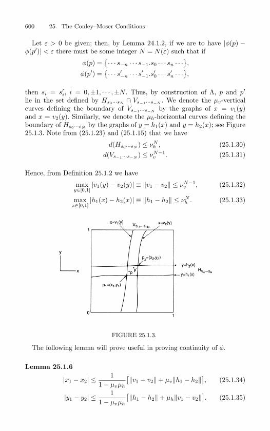
600 25. The Conley–Moser Conditions
Let ε > 0 be given; then, by Lemma 24.1.2, if we are to have |φ(p) −φ(p′)| < ε there must be some integer N = N(ε) such that if
φ(p) =· · · s−n · · · s−1.s0 · · · sn · · ·
,
φ(p′) =· · · s′
−n · · · s′−1.s
′0 · · · s′
n · · ·,
then si = s′i, i = 0,±1, · · · ,±N . Thus, by construction of Λ, p and p′
lie in the set defined by Hs0···sN∩ Vs−1···s−N
. We denote the µv-verticalcurves defining the boundary of Vs−1···s−N
by the graphs of x = v1(y)and x = v2(y). Similarly, we denote the µh-horizontal curves defining theboundary of Hs0···sN
by the graphs of y = h1(x) and y = h2(x); see Figure25.1.3. Note from (25.1.23) and (25.1.15) that we have
d(Hs0···sN) ≤ νN
h , (25.1.30)d(Vs−1···s−N
) ≤ νN−1v . (25.1.31)
Hence, from Definition 25.1.2 we have
maxy∈[0,1]
|v1(y)− v2(y)| ≡ ‖v1 − v2‖ ≤ νN−1v , (25.1.32)
maxx∈[0,1]
|h1(x)− h2(x)| ≡ ‖h1 − h2‖ ≤ νNh . (25.1.33)
FIGURE 25.1.3.
The following lemma will prove useful in proving continuity of φ.
Lemma 25.1.6
|x1 − x2| ≤1
1− µvµh
[‖v1 − v2‖+ µv‖h1 − h2‖
], (25.1.34)
|y1 − y2| ≤1
1− µvµh
[‖h1 − h2‖+ µh‖v1 − v2‖
]. (25.1.35)
25.1 The Main Theorem 601
Proof: This follows from the following simple calculations.
|x1 − x2| = |v1(y1)− v2(y2)|≤ |v1(y1)− v1(y2)|+ |v1(y2)− v2(y2)|≤ µv|y1 − y2|+ ‖v1 − v2‖ (25.1.36)
and|y1 − y2| = |h1(x1)− h2(x2)|
≤ |h1(x1)− h1(x2)|+ |h1(x2)− h2(x2)|≤ µh|x1 − x2|+ ‖h1 − h2‖. (25.1.37)
Substituting (25.1.37) into (25.1.36) gives (25.1.34), and substituting(25.1.36) into (25.1.37) gives (25.1.35). Note that these algebraic manipu-lations require 1− µvµh > 0. This proves Lemma 25.1.6.
Now we can complete the proof that φ is continuous. Let p1 denote theintersection of the graph of h1(x) with v1(y) and p2 denote the intersectionof the graph of h2(x) with v2(y). Now it follows that
|p− p′| ≤ |p1 − p2|. (25.1.38)
We denote the coordinates of p1 and p2 by (x1, y1) and (x2, y2), respectively.Using (25.1.38), we obtain
|p− p′| ≤ |x1 − x2|+ |y1 − y2|, (25.1.39)
and using Lemma 25.1.6, we obtain
|x1 − x2|+ |y1 − y2| ≤1
1− µvµh
[(1 + µh)‖v1 − v2‖
+ (1 + µv)‖h1 − h2‖]. (25.1.40)
Using (25.1.39), (25.1.40), (25.1.32), and (25.1.33) we obtain
|p− p′| ≤ 11− µvµh
[(1 + µh)νN−1
v + (1 + µv)νNh
].
Hence, if we take
δ =1
1− µvµh
[(1 + µh)νN−1
v + (1 + µv)νNh
],
continuity is proved.
602 25. The Conley–Moser Conditions
Step 4: φ f = σ φ. Choose any p ∈ Λ and let
φ(p) =· · · s−k · · · s−1.s0s1 · · · sk · · ·
;
thenσ φ(p) =
· · · s−k · · · s−1s0.s1 · · · sk · · ·
. (25.1.41)
Now, by definition of φ, it follows that
φ f(p) =· · · s−k · · · s−1s0.s1 · · · sk · · ·
; (25.1.42)
hence, from (25.1.41) and (25.1.42), we see that
φ f(p) = σ φ(p)
and p is arbitrary. This completes our proof of Theorem 25.1.5.
25.2 Sector Bundles
In Chapters 26 and 27 we will see that certain orbits called homoclinic orbitsgive rise to the geometrical conditions that allow Assumption 1 to hold ina two-dimensional map. However, a direct verification of Assumption 2 isnot easy. When one thinks of stretching and contraction rates of maps, it isnatural to think of the properties of the derivative of the map at differentpoints. We now want to derive a condition that is equivalent to Assumption2 that is based solely on properties of the derivative of f (hence we mustassume that f is at least C1). We begin by establishing some notation.
We definef(Hi) ∩Hj ≡ Vji (25.2.1)
andHi ∩ f−1(Hj) ≡ Hij = f−1(Vji) (25.2.2)
for i, j ∈ S where S = 1, . . . , N (N ≥ 2) is an index set; see Figure25.2.1. We further define
H =⋃
i,j∈S
Hij
and
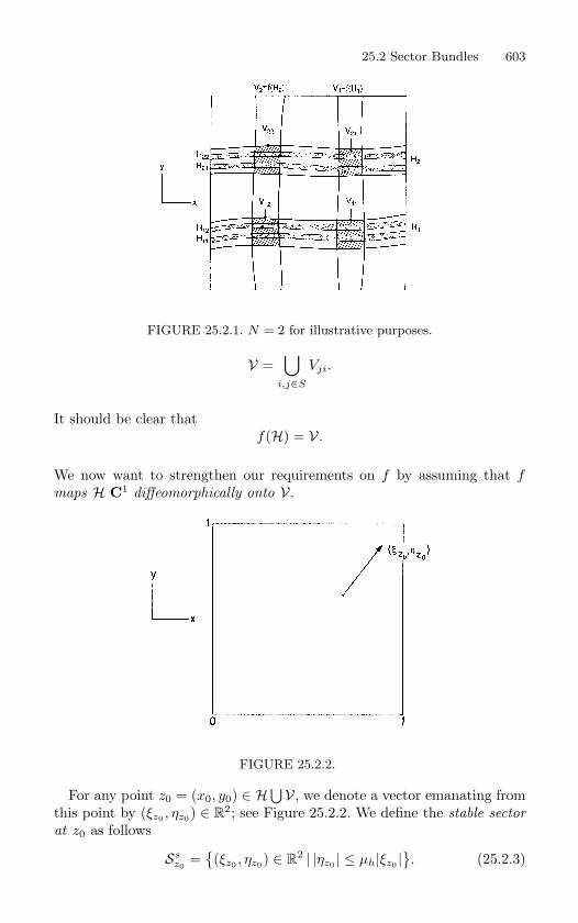
25.2 Sector Bundles 603
FIGURE 25.2.1. N = 2 for illustrative purposes.
V =⋃
i,j∈S
Vji.
It should be clear thatf(H) = V.
We now want to strengthen our requirements on f by assuming that fmaps H C1 diffeomorphically onto V.
FIGURE 25.2.2.
For any point z0 = (x0, y0) ∈ H⋃V, we denote a vector emanating from
this point by (ξz0 , ηz0) ∈ R2; see Figure 25.2.2. We define the stable sector
at z0 as follows
Ssz0
=(ξz0 , ηz0) ∈ R
2 | |ηz0 | ≤ µh|ξz0 |. (25.2.3)
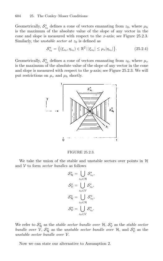
604 25. The Conley–Moser Conditions
Geometrically, Ssz0
defines a cone of vectors emanating from z0, where µh
is the maximum of the absolute value of the slope of any vector in thecone and slope is measured with respect to the x-axis; see Figure 25.2.3.Similarly, the unstable sector at z0 is defined as
Suz0
=(ξz0 , ηz0) ∈ R
2 | |ξz0 | ≤ µv|ηz0 |. (25.2.4)
Geometrically, Suz0
defines a cone of vectors emanating from z0, where µv
is the maximum of the absolute value of the slope of any vector in the coneand slope is measured with respect to the y-axis; see Figure 25.2.3. We willput restrictions on µv and µh shortly.
FIGURE 25.2.3.
We take the union of the stable and unstable sectors over points in Hand V to form sector bundles as follows
SsH =
⋃z0∈H
Ssz0
,
SsV =
⋃z0∈V
Ssz0
,
SuH =
⋃z0∈H
Suz0
,
SuV =
⋃z0∈V
Suz0
.
We refer to SsH as the stable sector bundle over H, Ss
V as the stable sector
bundle over V, SuH as the unstable sector bundle over H, and Su
V as theunstable sector bundle over V.
Now we can state our alternative to Assumption 2.
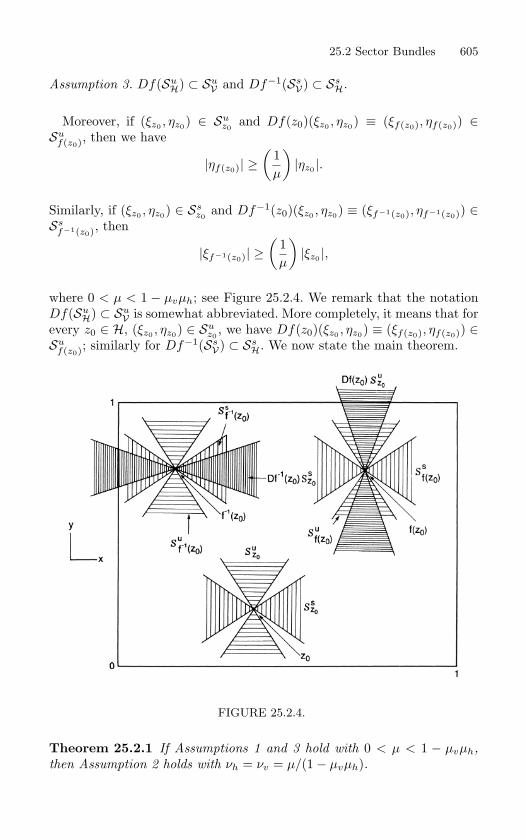
25.2 Sector Bundles 605
Assumption 3. Df(SuH) ⊂ Su
V and Df−1(SsV) ⊂ Ss
H.
Moreover, if (ξz0 , ηz0) ∈ Suz0
and Df(z0)(ξz0 , ηz0) ≡ (ξf(z0), ηf(z0)) ∈Su
f(z0), then we have
|ηf(z0)| ≥(
1µ
)|ηz0 |.
Similarly, if (ξz0 , ηz0) ∈ Ssz0
and Df−1(z0)(ξz0 , ηz0) ≡ (ξf−1(z0), ηf−1(z0)) ∈Ss
f−1(z0), then
|ξf−1(z0)| ≥(
1µ
)|ξz0 |,
where 0 < µ < 1 − µvµh; see Figure 25.2.4. We remark that the notationDf(Su
H) ⊂ SuV is somewhat abbreviated. More completely, it means that for
every z0 ∈ H, (ξz0 , ηz0) ∈ Suz0
, we have Df(z0)(ξz0 , ηz0) ≡ (ξf(z0), ηf(z0)) ∈Su
f(z0); similarly for Df−1(SsV) ⊂ Ss
H. We now state the main theorem.
FIGURE 25.2.4.
Theorem 25.2.1 If Assumptions 1 and 3 hold with 0 < µ < 1 − µvµh,
then Assumption 2 holds with νh = νv = µ/(1− µvµh).
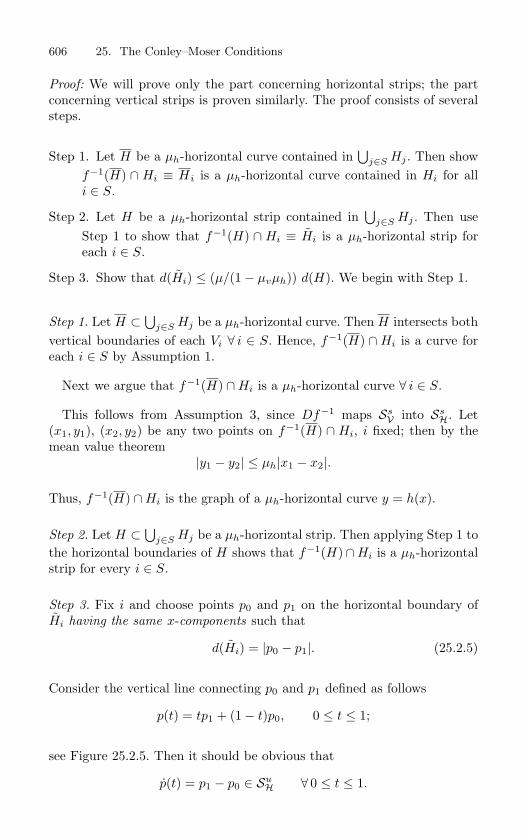
606 25. The Conley–Moser Conditions
Proof: We will prove only the part concerning horizontal strips; the partconcerning vertical strips is proven similarly. The proof consists of severalsteps.
Step 1. Let H be a µh-horizontal curve contained in⋃
j∈S Hj . Then showf−1(H) ∩ Hi ≡ Hi is a µh-horizontal curve contained in Hi for alli ∈ S.
Step 2. Let H be a µh-horizontal strip contained in⋃
j∈S Hj . Then useStep 1 to show that f−1(H) ∩ Hi ≡ Hi is a µh-horizontal strip foreach i ∈ S.
Step 3. Show that d(Hi) ≤ (µ/(1− µvµh)) d(H). We begin with Step 1.
Step 1. Let H ⊂⋃
j∈S Hj be a µh-horizontal curve. Then H intersects bothvertical boundaries of each Vi ∀ i ∈ S. Hence, f−1(H) ∩Hi is a curve foreach i ∈ S by Assumption 1.
Next we argue that f−1(H) ∩Hi is a µh-horizontal curve ∀ i ∈ S.
This follows from Assumption 3, since Df−1 maps SsV into Ss
H. Let(x1, y1), (x2, y2) be any two points on f−1(H) ∩ Hi, i fixed; then by themean value theorem
|y1 − y2| ≤ µh|x1 − x2|.
Thus, f−1(H) ∩Hi is the graph of a µh-horizontal curve y = h(x).
Step 2. Let H ⊂⋃
j∈S Hj be a µh-horizontal strip. Then applying Step 1 tothe horizontal boundaries of H shows that f−1(H)∩Hi is a µh-horizontalstrip for every i ∈ S.
Step 3. Fix i and choose points p0 and p1 on the horizontal boundary ofHi having the same x-components such that
d(Hi) = |p0 − p1|. (25.2.5)
Consider the vertical line connecting p0 and p1 defined as follows
p(t) = tp1 + (1− t)p0, 0 ≤ t ≤ 1;
see Figure 25.2.5. Then it should be obvious that
p(t) = p1 − p0 ∈ SuH ∀ 0 ≤ t ≤ 1.
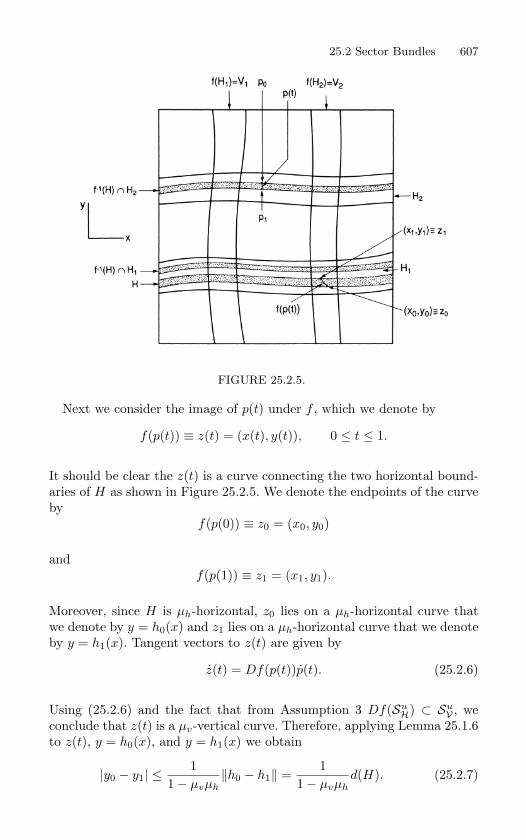
25.2 Sector Bundles 607
FIGURE 25.2.5.
Next we consider the image of p(t) under f , which we denote by
f(p(t)) ≡ z(t) = (x(t), y(t)), 0 ≤ t ≤ 1.
It should be clear the z(t) is a curve connecting the two horizontal bound-aries of H as shown in Figure 25.2.5. We denote the endpoints of the curveby
f(p(0)) ≡ z0 = (x0, y0)
andf(p(1)) ≡ z1 = (x1, y1).
Moreover, since H is µh-horizontal, z0 lies on a µh-horizontal curve thatwe denote by y = h0(x) and z1 lies on a µh-horizontal curve that we denoteby y = h1(x). Tangent vectors to z(t) are given by
z(t) = Df(p(t))p(t). (25.2.6)
Using (25.2.6) and the fact that from Assumption 3 Df(SuH) ⊂ Su
V , weconclude that z(t) is a µv-vertical curve. Therefore, applying Lemma 25.1.6to z(t), y = h0(x), and y = h1(x) we obtain
|y0 − y1| ≤1
1− µvµh‖h0 − h1‖ =
11− µvµh
d(H). (25.2.7)
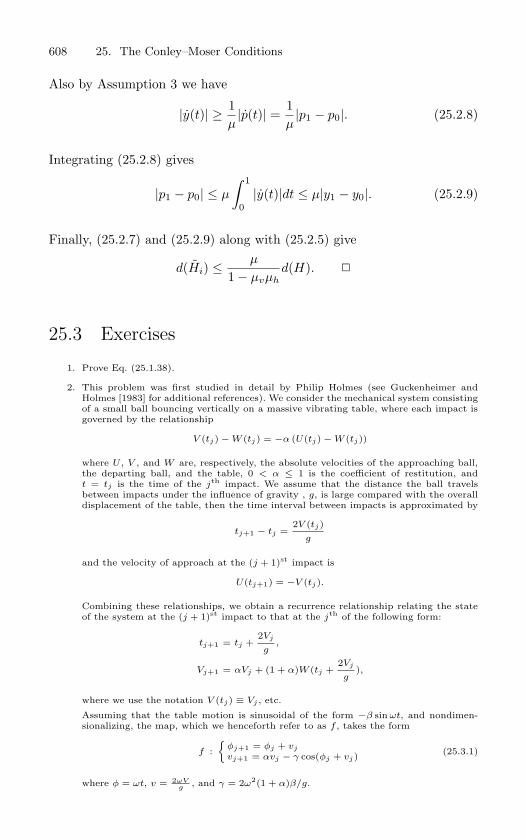
608 25. The Conley–Moser Conditions
Also by Assumption 3 we have
|y(t)| ≥ 1µ|p(t)| = 1
µ|p1 − p0|. (25.2.8)
Integrating (25.2.8) gives
|p1 − p0| ≤ µ
∫ 1
0|y(t)|dt ≤ µ|y1 − y0|. (25.2.9)
Finally, (25.2.7) and (25.2.9) along with (25.2.5) give
d(Hi) ≤µ
1− µvµhd(H).
25.3 Exercises
1. Prove Eq. (25.1.38).
2. This problem was first studied in detail by Philip Holmes (see Guckenheimer andHolmes [1983] for additional references). We consider the mechanical system consistingof a small ball bouncing vertically on a massive vibrating table, where each impact isgoverned by the relationship
V (tj) − W (tj) = −α (U(tj) − W (tj))
where U , V , and W are, respectively, the absolute velocities of the approaching ball,the departing ball, and the table, 0 < α ≤ 1 is the coefficient of restitution, andt = tj is the time of the jth impact. We assume that the distance the ball travelsbetween impacts under the influence of gravity , g, is large compared with the overalldisplacement of the table, then the time interval between impacts is approximated by
tj+1 − tj =2V (tj)
g
and the velocity of approach at the (j + 1)st impact is
U(tj+1) = −V (tj).
Combining these relationships, we obtain a recurrence relationship relating the stateof the system at the (j + 1)st impact to that at the jth of the following form:
tj+1 = tj +2Vj
g,
Vj+1 = αVj + (1 + α)W (tj +2Vj
g),
where we use the notation V (tj) ≡ Vj , etc.
Assuming that the table motion is sinusoidal of the form −β sin ωt, and nondimen-sionalizing, the map, which we henceforth refer to as f , takes the form
f :
φj+1 = φj + vj
vj+1 = αvj − γ cos(φj + vj)(25.3.1)
where φ = ωt, v = 2ωVg , and γ = 2ω2(1 + α)β/g.
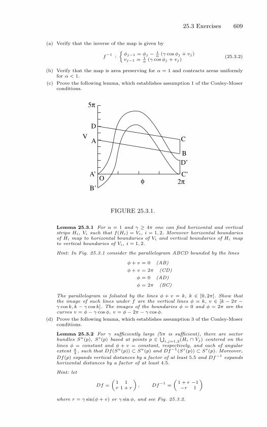
25.3 Exercises 609
(a) Verify that the inverse of the map is given by
f−1 :
φj−1 = φj − 1
α (γ cos φj + vj)vj−1 = 1
α (γ cos φj + vj)(25.3.2)
(b) Verify that the map is area preserving for α = 1 and contracts areas uniformlyfor α < 1.
(c) Prove the following lemma, which establishes assumption 1 of the Conley-Moserconditions.
A
A’
B
B’
C
C’
D
D’
O
V
φ
5π
2π
FIGURE 25.3.1.
Lemma 25.3.1 For α = 1 and γ ≥ 4π one can find horizontal and verticalstrips Hi, Vi such that f(Hi) = Vi, i = 1, 2. Moreover horizontal boundariesof Hi map to horizontal boundaries of Vi and vertical boundaries of Hi mapto vertical boundaries of Vi, i = 1, 2.
Hint: In Fig. 25.3.1 consider the parallelogram ABCD bounded by the lines
φ + v = 0 (AB)
φ + v = 2π (CD)
φ = 0 (AD)
φ = 2π (BC)
The parallelogram is foliated by the lines φ + v = k, k ∈ [0, 2π]. Show thatthe image of such lines under f are the vertical lines φ = k, v ∈ [k − 2π −γ cos k, k − γ cos k]. The images of the boundaries φ = 0 and φ = 2π are thecurves v = φ − γ cos φ, v = φ − 2π − γ cos φ.
(d) Prove the following lemma, which establishes assumption 3 of the Conley-Moserconditions.
Lemma 25.3.2 For γ sufficiently large (5π is sufficient), there are sectorbundles Su(p), Ss(p) based at points p ∈
⋃i,j=1,2(Hi ∩ Vj) centered on the
lines φ = constant and φ + v = constant, respectively, and each of angularextent π
4 , such that Df(Su(p)) ⊂ Su(p) and Df−1(Ss(p)) ⊂ Ss(p). Moreover,Df(p) expands vertical distances by a factor of at least 5.5 and Df−1 expandshorizontal distances by a factor of at least 4.5.
Hint: let
Df =(
1 1r 1 + r
), Df
−1 =(
1 + r −1−r 1
)
where r = γ sin(φ + v) or γ sin φ, and see Fig. 25.3.2.
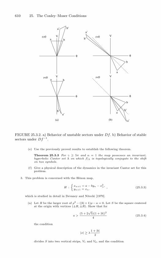
610 25. The Conley–Moser Conditions
V
φ
r>0
r<0 V
φ
r>0
V
φ
V
φ
r<0
a
b
a’
b’
a
a
a
b
b
b
a’
a’
a’
b’b’
b’
(a) (b)
FIGURE 25.3.2. a) Behavior of unstable sectors under Df . b) Behavior of stable
sectors under Df−1.
(e) Use the previously proved results to establish the following theorem.
Theorem 25.3.3 For γ ≥ 5π and α = 1 the map possesses an invariant,hyperbolic Cantor set Λ on which f |Λ is topologically conjugate to the shifton two symbols.
(f) Give a physical description of the dynamics in the invariant Cantor set for thisproblem.
3. This problem is concerned with the Henon map,
H :
xn+1 = a − byn − x2n,
yn+1 = xn., (25.3.3)
which is studied in detail in Devaney and Nitecki [1979].
(a) Let R be the larger root of ρ2 − (|b| + 1)ρ − a = 0. Let S be the square centeredat the origin with vertices (±R, ±R). Show that for
a >(5 + 2
√5)(1 + |b|)2
4(25.3.4)
the condition
|x| ≥ λ1 + |b|
2
divides S into two vertical strips, V1 and V2, and the condition
25.3 Exercises 611
|y| ≥ λ1 + |b|
2
divides S into two horizontal strips, H1 and H2, which obey assumption 1 ofthe Conley-Moser conditions.
(b) Consider the sectors
Suz0
=(ξz0 , ηz0 ) | |ξz0 | ≥ λ|ηz0 |
,
Ssz0
=(ξz0 , ηz0 ) | |ηz0 | ≥ λ|ξz0 |
.
Prove that if (25.3.4) holds then we can choose λ > 2 so that in V1 and V2Su is invariant under DH(x, y) and in the H1 and H2 Ss is invariant underDH−1(x, y). Thus, conclude that assumption 3 of the Conley-Moser Conditionshold.
(c) Prove that the Henon map has a hyperbolic invariant Cantor set on which it istopologically conjugate to the shift on two symbols.
4. Horseshoes are Structurally Stable. Suppose that a map f : D → R2 satisfies the
hypothesis of Theorem 25.2.1. Then it possesses an invariant Cantor set Λ. Show that,for ε sufficiently small, the map f + εg (with g Cr, r ≥ 1, on D) also possesses an
invariant Cantor set Λε. Moreover, show that Λε can be constructed so that (f +εg)∣∣∣Λε
is topologically conjugate to f∣∣∣Λ.
26
Dynamics Near HomoclinicPoints of Two-DimensionalMaps
In Chapter 25 we gave sufficient conditions for a two-dimensional mapto possess an invariant Cantor set on which it is topologically conjugateto a full shift on N symbols. In this section we want to show that theexistence of certain orbits of a two-dimensional map, specifically, transversehomoclinic orbits to a hyperbolic fixed point, imply that in a sufficientlysmall neighborhood of a point on the homoclinic orbit, the conditions givenin Chapter 25 hold. There are two very similar theorems which deal withthis situation; Moser’s theorem (see Moser [1973]) and the Smale–Birkhoffhomoclinic theorem (see Smale [1963]). We will prove Moser’s theorem anddescribe how the Smale–Birkhoff theorem differs.
The situation that we are considering is as follows: let
f : R2 −→ R2
be a Cr (r ≥ 1) diffeomorphism satisfying the following hypotheses.
Hypothesis 1. f has a hyperbolic periodic point, p.
Hypothesis 2. W s(p) and Wu(p) intersect transversely.
Without loss of generality we can assume that the hyperbolic periodicpoint, p, is a fixed point, for if p has period k, then fk(p) = p and thefollowing arguments can be applied to fk. A point that is in W s(p)∩Wu(p)is said to be homoclinic to p. If W s(p) intersects Wu(p) transversely in apoint, then the point is called a transverse homoclinic point. Our goal is toshow that in a neighborhood of a transverse homoclinic point there existsan invariant Cantor set on which the dynamics are topologically conjugateto a full shift on N symbols. Before formulating this as a theorem, a fewpreliminary steps need to be taken.
26. Dynamics Near Homoclinic Points of Two-Dimensional Maps 613
Step 1: Local Coordinates for f . Without loss of generality we can assumethat the hyperbolic fixed point, p, is located at the origin (cf. Section 3).Let U be a neighborhood of the origin. Then, in U , f can be written in theform
ξ −→ λξ + g1(ξ, η),η −→ µη + g2(ξ, η), (ξ, η) ∈ U ⊂ R
2, (26.0.1)
where 0 < |λ| < 1, |µ| > 1, and g1, g2 are O(2) in ξ and η. Hence, η = 0 andξ = 0 are the stable and unstable manifolds, respectively, of the linearized
map. However, in the proof of the theorem we will find it more convenientto use the local stable and unstable manifolds of the origin as coordinates.This can be done by utilizing a simple (nonlinear) change of coordinates.
We know from Theorem 3.2.1 that the local stable and unstable mani-folds of the hyperbolic fixed point can be represented as the graphs of Cr
functions, i.e.,W s
loc(0) = graph hs(ξ),Wu
loc(0) = graph hu(η), (26.0.2)
where hs(0) = hu(0) = Dhs(0) = Dhu(0) = 0. If we define the coordinatetransformation
(x, y) = (ξ − hu(η), η − hs(ξ)), (26.0.3)
then (26.0.1) takes the form
x −→ λx + f1(x, y),y −→ µy + f2(x, y), (26.0.4)
withf1(0, y) = 0,f2(x, 0) = 0. (26.0.5)
Equation (26.0.5) implies that y = 0 and x = 0 are the stable and unstablemanifolds, respectively, of the origin. We emphasize that the transforma-tion (26.0.3) is only locally valid; therefore (26.0.4) has meaning only in a“sufficiently small” neighborhood of the origin. Despite the bad notation,we refer to this neighborhood, as above, by U .
Step 2: Global Consequences of a Homoclinic Orbit. By assumption, W s(0)and Wu(0) intersect at, say, q. Then, since q ∈ W s(0) ∩Wu(0),
limn→∞
fn(q) = 0,
limn→−∞
fn(q) = 0. (26.0.6)
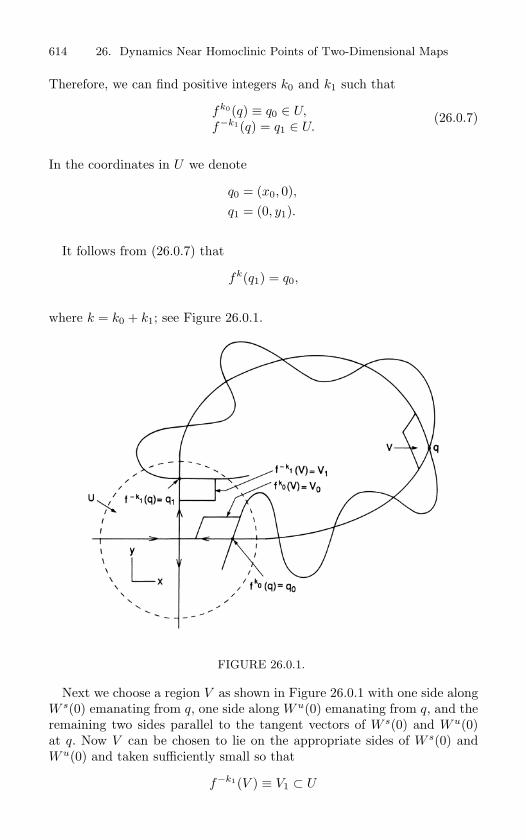
614 26. Dynamics Near Homoclinic Points of Two-Dimensional Maps
Therefore, we can find positive integers k0 and k1 such that
fk0(q) ≡ q0 ∈ U,f−k1(q) = q1 ∈ U.
(26.0.7)
In the coordinates in U we denote
q0 = (x0, 0),q1 = (0, y1).
It follows from (26.0.7) that
fk(q1) = q0,
where k = k0 + k1; see Figure 26.0.1.
FIGURE 26.0.1.
Next we choose a region V as shown in Figure 26.0.1 with one side alongW s(0) emanating from q, one side along Wu(0) emanating from q, and theremaining two sides parallel to the tangent vectors of W s(0) and Wu(0)at q. Now V can be chosen to lie on the appropriate sides of W s(0) andWu(0) and taken sufficiently small so that
f−k1(V ) ≡ V1 ⊂ U
26. Dynamics Near Homoclinic Points of Two-Dimensional Maps 615
andfk0(V ) ≡ V0 ⊂ U (26.0.8)
appear as in Figure 26.0.1. From (26.0.8) it follows that we have
fk(V1) = V0. (26.0.9)
Let us make an important comment concerning Figure 26.0.1. The im-portant aspect is that we can choose V and (large) positive integers k0 andk1 such that fk0(V ) and f−k1(V ) are both in the first quadrant, and dis-
joint. This can always be done and is left as one of the exercises at the endof this section. (Note: Certainly k depends on the size of U as U shrinksto a point k → ∞.) We remark that in Figure 26.0.1 we depict W s(0)and Wu(0) as winding amongst each other. We will discuss the geometricalaspects of this more fully later on; for the proof of this theorem a detailedknowledge of the geometry of the “homoclinic tangle” is not so important.However, the one aspect of the intersection of W s(0) and Wu(0) at q thatwill be of importance is the assumption that the intersection is transversal
at q. Since f is a diffeomorphism, this implies that W s(0) and Wu(0) alsointersect transversely at fk0(q) = q0 and f−k1(q) = q1 (or, more generally,at fk(q) for any integer k).
The next step involves gaining an understanding of the dynamics nearthe hyperbolic fixed point.
Step 3: Dynamics Near the Origin. We first state a well-known lemma thatdescribes some geometric aspects of the dynamics of a curve as it passesnear the hyperbolic fixed point under iteration by f .
Let q ∈ W s(0)−0, and let C be a curve intersecting W s(0) transverselyat q. Let CN denote the connected component of fN (C)∩U to which fN (q)belongs; see Figure 26.0.2. Then we have the following lemma.
Lemma 26.0.4 (The lambda lemma) Given ε > 0 and U sufficiently
small there exists a positive integer N0 such that for N ≥ N0 CN is C1
ε-close to Wu(0) ∩ U .
Proof: Proofs can be found in Palis and de Melo [1982] or Newhouse [1980].Here we give a proof for two-dimensional diffeomorphisms.
Without loss of generality we can assume q ∈ U . Moreover, we will takeU of the form
U ≡ Ix × Iy,
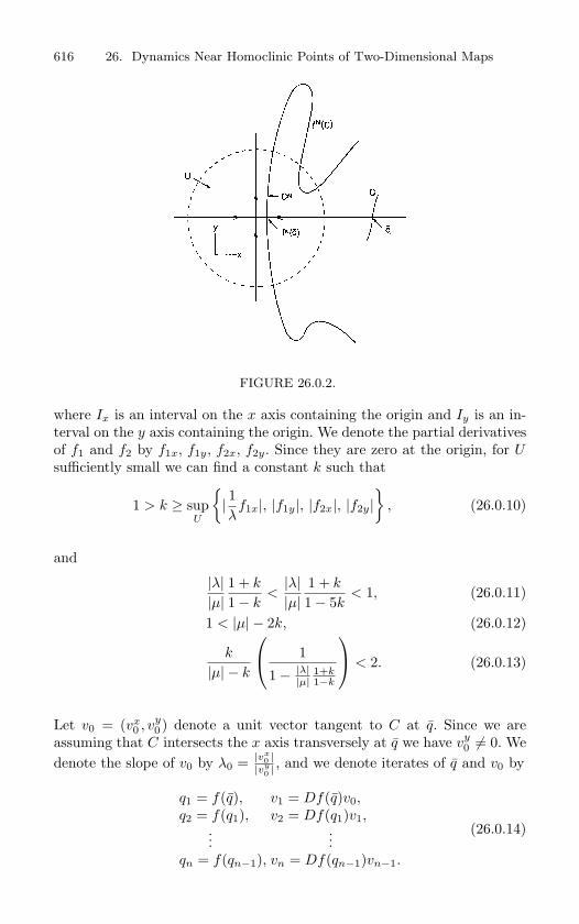
616 26. Dynamics Near Homoclinic Points of Two-Dimensional Maps
FIGURE 26.0.2.
where Ix is an interval on the x axis containing the origin and Iy is an in-terval on the y axis containing the origin. We denote the partial derivativesof f1 and f2 by f1x, f1y, f2x, f2y. Since they are zero at the origin, for Usufficiently small we can find a constant k such that
1 > k ≥ supU
| 1λ
f1x|, |f1y|, |f2x|, |f2y|
, (26.0.10)
and
|λ||µ|
1 + k
1− k<|λ||µ|
1 + k
1− 5k< 1, (26.0.11)
1 < |µ| − 2k, (26.0.12)
k
|µ| − k
1
1− |λ||µ|
1+k1−k
< 2. (26.0.13)
Let v0 = (vx0 , vy
0 ) denote a unit vector tangent to C at q. Since we areassuming that C intersects the x axis transversely at q we have vy
0 = 0. Wedenote the slope of v0 by λ0 = |vx
0 ||vy
0 | , and we denote iterates of q and v0 by
q1 = f(q), v1 = Df(q)v0,q2 = f(q1), v2 = Df(q1)v1,
......
qn = f(qn−1), vn = Df(qn−1)vn−1.
(26.0.14)
26. Dynamics Near Homoclinic Points of Two-Dimensional Maps 617
The steps in the proof of the lemma are as follows.
Step 1. Estimate the slopes of the iterates of v0 under Df and show thatthey are bounded for all n ≥ n0.
Step 2. The estimates of step 1 are for a vector tangent to C at q. Usingcontinuity of tangent vectors with respect to the point of tangency, weextend the estimates of step 1 to all tangent vectors in some smallercurve, C, contained in fn0(C) that passes through fn0(q). We thenestimate the slopes of an arbitrary vector on C under iteration byDf .
Step 3. Once the estimates for the slopes of iterates of tangent vectorsto C are obtained we then show that C stretches in the direction ofWu(0) ∩ U under iteration by f .
We begin with the first step. We estimate the evolution of the slope ofv0 under iteration by Df . We have
Df(q)v0 =(
λ + f1x(x, 0) f1y(x, 0)0 µ + f2y(x, 0)
)(vx0
vy0
),
=(
(λ + f1x(x, 0)) vx0 + f1y(x, 0)vy
0(µ + f2y(x, 0)) vy
0
)≡
(vx1
vy1
),(26.0.15)
where the zero entry in the matrix arises since f2(x, 0) = f2x(x, 0) = 0.Using (26.0.15) and (26.0.10), we obtain the following estimates
λ1 =|vx
1 ||vy
1 |=|λvx
0 + f1xvx0 + f1yvy
0 ||µvy
0 + f2yvy0 |
,
≤ |λvx0 + f1xvx
0 ||µvy
0 + f2yvy0 |
+|f1y|
|µ + f2y|,
≤ |λ||µ||vx
0 ||vy
0 ||1 + f1x
λ ||1 + f2y
µ |+
|f1y||µ + f2y|
,
≤ |λ||µ|λ0
1 + k
1− k+
k
|µ| − k. (26.0.16)
Henceforth we will not explicitly denote the arguments of the partial
derivatives f1x, f1y, f2x, f2y as we will always estimate them using the
uniform estimate in (26.0.10). This will always apply since they will
always be evaluated on points in U .
Repeating the calculation in (26.0.15), and the estimates used in (26.0.16)gives
618 26. Dynamics Near Homoclinic Points of Two-Dimensional Maps
λ2 =|vx
2 ||vy
2 |=|λvx
1 + f1xvx1 + f1yvy
1 ||µvy
1 + f2yvy1 |
,
≤ |λ||µ|λ1
1 + k
1− k+
k
|µ| − k, (26.0.17)
Repeating these same calculations and estimates, at the nth step we obtainthe following estimate
λn ≤|λ||µ|λn−1
1 + k
1− k+
k
|µ| − k, (26.0.18)
or,
λn ≤( |λ||µ|
1 + k
1− k
)n
λ0 +k
|µ| − k
n−1∑i=0
( |λ||µ|
1 + k
1− k
)i
,
≤( |λ||µ|
1 + k
1− k
)n
λ0 +k
|µ| − k
1
1− |λ||µ|
1+k1−k
. (26.0.19)
Since, by (26.0.11),(
|λ||µ|
1+k1−k
)n
→ 0 as n → ∞ we can find an integer n0
such thatλn ≤ 3 for all n ≥ n0. (26.0.20)
This completes step 1.
In step 2 we begin by considering a smaller neighborhood of the origin,but one that is only shrunk in the x direction. Let δ be a small positivereal number and let δIx denote Ix multiplied or “scaled” by δ. Let
U1 ≡ δIx × Iy.
Then we can choose δ so small that
supU1
|f1y| ≤ k1 (26.0.21)
where
k1 ≤ε
2(|µ| − 5k)
(1− |λ|
|µ|1 + k
1− 5k
). (26.0.22)
By continuity of tangent vectors, we can find a curve in fn0(C), C,containing fn0(q), such that the slope λ of any unit vector on this curveobeys
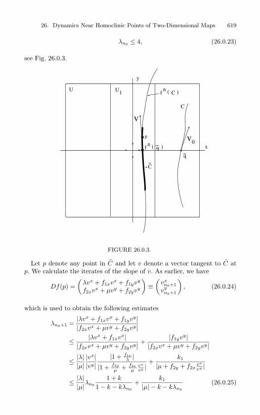
26. Dynamics Near Homoclinic Points of Two-Dimensional Maps 619
λn0 ≤ 4, (26.0.23)
see Fig. 26.0.3.
x
y
q( )fn
q
C
C
~
v0
UU 1
v
p
( )fn
C
FIGURE 26.0.3.
Let p denote any point in C and let v denote a vector tangent to C atp. We calculate the iterates of the slope of v. As earlier, we have
Df(p) =(
λvx + f1xvx + f1yvy
f2xvx + µvy + f2yvy
)≡
(vx
n0+1vy
n0+1
), (26.0.24)
which is used to obtain the following estimates
λn0+1 =|λvx + f1xvx + f1yvy||f2xvx + µvy + f2yvy|
≤ |λvx + f1xvx||f2xvx + µvy + f2yvy| +
|f1yvy||f2xvx + µvy + f2yvy|
≤ |λ||µ||vx||vy|
|1 + f1x
λ ||1 + f2y
µ + f2x
µvx
vy |+
k1
|µ + f2y + f2xvx
vy |
≤ |λ||µ|λn0
1 + k
1− k − kλn0
+k1
|µ| − k − kλn0
(26.0.25)
620 26. Dynamics Near Homoclinic Points of Two-Dimensional Maps
or, using (26.0.23),
λn0+1 ≤|λ||µ|λn0
1 + k
1− 5k+
k1
|µ| − 5k. (26.0.26)
Iterating these calculations as above gives
λn0+n ≤( |λ||µ|
1 + k
1− 5k
)n
λn0 +k1
µ− 5k
1
1− |λ||µ|
1+k1−5k
. (26.0.27)
Since(
|λ||µ|
1+k1−5k
)n
→ 0 as n →∞, and λn0 is bounded by (26.0.23), we canfind an integer n such that( |λ|
|µ|1 + k
1− 5k
)n
λn0 ≤ε
2
for n ≥ n. Using this, along with (26.0.22), gives
λn0+n ≤ ε (26.0.28)
for n ≥ n. Note that this calculation is valid for any tangent vector infn(C). We can take N0 in the statement of the lemma to be n0 + n. Thiscompletes step 2.
In step 3 we compare the norm of a tangent vector to that of its imageunder Df , i.e., we estimate√
|vxn+1|2 + |vy
n+1|2|vx
n|2 + |vyn|2
=|vy
n+1||vy
n|
√λ2
n+1 + 1λ2
n + 1. (26.0.29)
For n sufficiently large this expression is arbitrarily close to|vy
n+1||vy
n| sinceλn → 0 as n →∞. We also have that
|vyn+1||vy
n|=|f2xvx
n + µvyn + f2yvy
n||vy
n|= |f2xλn + µ + f2y| > |µ| − 2k > 1 (26.0.30)
for n large by (26.0.12) and (26.0.28). Thus we see that the norms of theiterates of nonzero tangent vectors are growing by a ratio that approaches|µ| − 2k > 1. Hence, fn(C) is stretching in the direction of Wu(0) ∩ U .This, together with (26.0.28), proves the lemma.
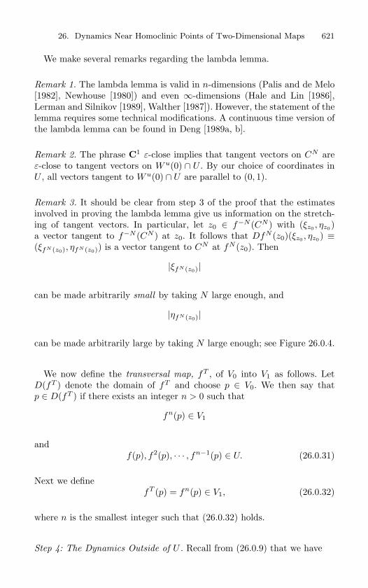
26. Dynamics Near Homoclinic Points of Two-Dimensional Maps 621
We make several remarks regarding the lambda lemma.
Remark 1. The lambda lemma is valid in n-dimensions (Palis and de Melo[1982], Newhouse [1980]) and even ∞-dimensions (Hale and Lin [1986],Lerman and Silnikov [1989], Walther [1987]). However, the statement of thelemma requires some technical modifications. A continuous time version ofthe lambda lemma can be found in Deng [1989a, b].
Remark 2. The phrase C1 ε-close implies that tangent vectors on CN areε-close to tangent vectors on Wu(0) ∩ U . By our choice of coordinates inU , all vectors tangent to Wu(0) ∩ U are parallel to (0, 1).
Remark 3. It should be clear from step 3 of the proof that the estimatesinvolved in proving the lambda lemma give us information on the stretch-ing of tangent vectors. In particular, let z0 ∈ f−N (CN ) with (ξz0 , ηz0)a vector tangent to f−N (CN ) at z0. It follows that DfN (z0)(ξz0 , ηz0) ≡(ξfN (z0), ηfN (z0)) is a vector tangent to CN at fN (z0). Then
|ξfN (z0)|
can be made arbitrarily small by taking N large enough, and
|ηfN (z0)|
can be made arbitrarily large by taking N large enough; see Figure 26.0.4.
We now define the transversal map, fT , of V0 into V1 as follows. LetD(fT ) denote the domain of fT and choose p ∈ V0. We then say thatp ∈ D(fT ) if there exists an integer n > 0 such that
fn(p) ∈ V1
andf(p), f2(p), · · · , fn−1(p) ∈ U. (26.0.31)
Next we definefT (p) = fn(p) ∈ V1, (26.0.32)
where n is the smallest integer such that (26.0.32) holds.
Step 4: The Dynamics Outside of U . Recall from (26.0.9) that we have
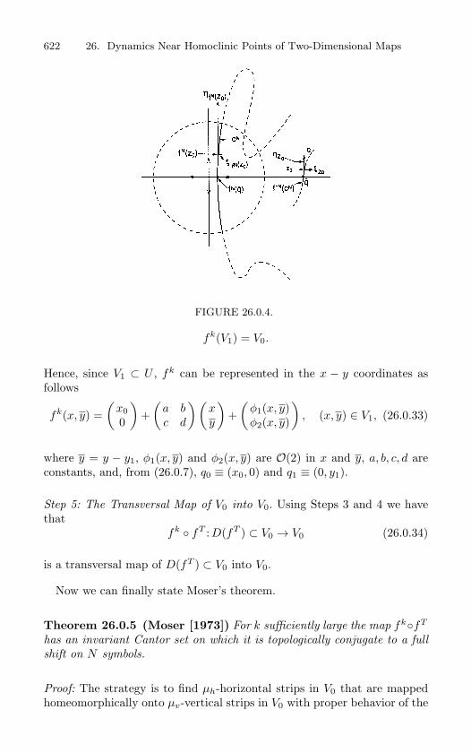
622 26. Dynamics Near Homoclinic Points of Two-Dimensional Maps
FIGURE 26.0.4.
fk(V1) = V0.
Hence, since V1 ⊂ U , fk can be represented in the x − y coordinates asfollows
fk(x, y) =(
x00
)+
(a bc d
)(xy
)+
(φ1(x, y)φ2(x, y)
), (x, y) ∈ V1, (26.0.33)
where y = y − y1, φ1(x, y) and φ2(x, y) are O(2) in x and y, a, b, c, d areconstants, and, from (26.0.7), q0 ≡ (x0, 0) and q1 ≡ (0, y1).
Step 5: The Transversal Map of V0 into V0. Using Steps 3 and 4 we havethat
fk fT :D(fT ) ⊂ V0 → V0 (26.0.34)
is a transversal map of D(fT ) ⊂ V0 into V0.
Now we can finally state Moser’s theorem.
Theorem 26.0.5 (Moser [1973]) For k sufficiently large the map fkfT
has an invariant Cantor set on which it is topologically conjugate to a full
shift on N symbols.
Proof: The strategy is to find µh-horizontal strips in V0 that are mappedhomeomorphically onto µv-vertical strips in V0 with proper behavior of the
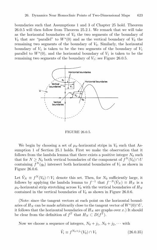
26. Dynamics Near Homoclinic Points of Two-Dimensional Maps 623
boundaries such that Assumptions 1 and 3 of Chapter 25 hold. Theorem26.0.5 will then follow from Theorem 25.2.1. We remark that we will takeas the horizontal boundaries of V0 the two segments of the boundary ofV0 that are “parallel” to W s(0) and as the vertical boundary of V0 theremaining two segments of the boundary of V0. Similarly, the horizontalboundary of V1 is taken to be the two segments of the boundary of V1parallel to W s(0), and the horizontal boundary of V1 is taken to be theremaining two segments of the boundary of V1; see Figure 26.0.5.
FIGURE 26.0.5.
We begin by choosing a set of µh-horizontal strips in V0 such that As-sumption 1 of Section 25.1 holds. First we make the observation that itfollows from the lambda lemma that there exists a positive integer N0 suchthat for N ≥ N0 both vertical boundaries of the component of fN (V0)∩Ucontaining fN (q0) intersect both horizontal boundaries of V1 as shown inFigure 26.0.6.
Let VN ≡ fN (V0) ∩ V1 denote this set. Then, for N0 sufficiently large, itfollows by applying the lambda lemma to f−1 that f−N (VN ) ≡ HN is aµh-horizontal strip stretching across V0 with the vertical boundaries of HN
contained in the vertical boundaries of V0 as shown in Figure 26.0.6.
(Note: since the tangent vectors at each point on the horizontal bound-aries of HN can be made arbitrarily close to the tangent vector of W s(0)∩U ,it follows that the horizontal boundaries of HN are graphs over x.) It shouldbe clear from the definition of fT that HN ⊂ D(fT ).
Now we choose a sequence of integers, N0 + j1, N0 + j2, · · · with
Vi ≡ fN0+ji(V0) ∩ V1 (26.0.35)
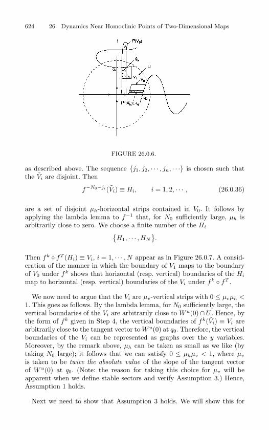
624 26. Dynamics Near Homoclinic Points of Two-Dimensional Maps
FIGURE 26.0.6.
as described above. The sequence j1, j2, · · · , jn, · · · is chosen such thatthe Vi are disjoint. Then
f−N0−ji(Vi) ≡ Hi, i = 1, 2, · · · , (26.0.36)
are a set of disjoint µh-horizontal strips contained in V0. It follows byapplying the lambda lemma to f−1 that, for N0 sufficiently large, µh isarbitrarily close to zero. We choose a finite number of the Hi
H1, · · · , HN
.
Then fk fT (Hi) ≡ Vi, i = 1, · · · , N appear as in Figure 26.0.7. A consid-eration of the manner in which the boundary of V1 maps to the boundaryof V0 under fk shows that horizontal (resp. vertical) boundaries of the Hi
map to horizontal (resp. vertical) boundaries of the Vi under fk fT .
We now need to argue that the Vi are µv-vertical strips with 0 ≤ µvµh <1. This goes as follows. By the lambda lemma, for N0 sufficiently large, thevertical boundaries of the Vi are arbitrarily close to Wu(0)∩U . Hence, bythe form of fk given in Step 4, the vertical boundaries of fk(Vi) ≡ Vi arearbitrarily close to the tangent vector to Wu(0) at q0. Therefore, the verticalboundaries of the Vi can be represented as graphs over the y variables.Moreover, by the remark above, µh can be taken as small as we like (bytaking N0 large); it follows that we can satisfy 0 ≤ µhµv < 1, where µv
is taken to be twice the absolute value of the slope of the tangent vectorof Wu(0) at q0. (Note: the reason for taking this choice for µv will beapparent when we define stable sectors and verify Assumption 3.) Hence,Assumption 1 holds.
Next we need to show that Assumption 3 holds. We will show this for
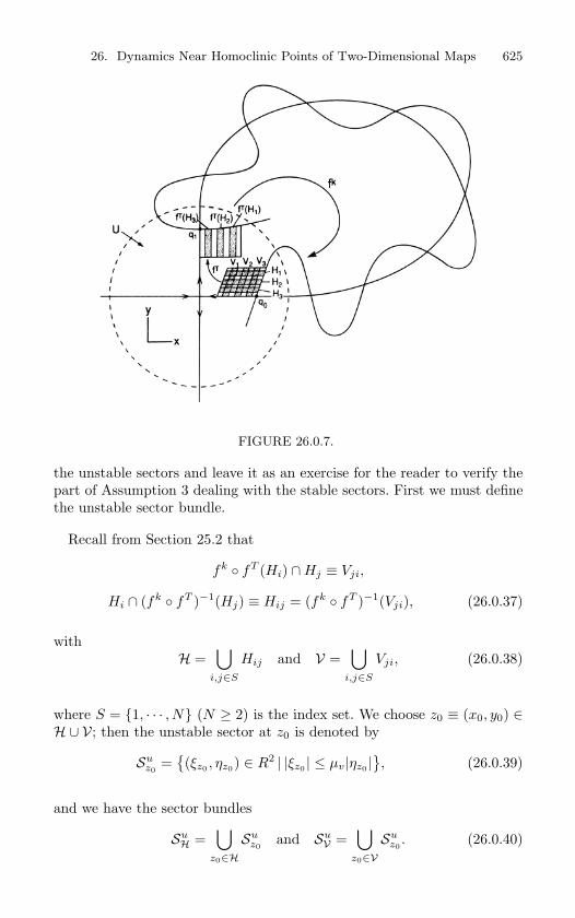
26. Dynamics Near Homoclinic Points of Two-Dimensional Maps 625
FIGURE 26.0.7.
the unstable sectors and leave it as an exercise for the reader to verify thepart of Assumption 3 dealing with the stable sectors. First we must definethe unstable sector bundle.
Recall from Section 25.2 that
fk fT (Hi) ∩Hj ≡ Vji,
Hi ∩ (fk fT )−1(Hj) ≡ Hij = (fk fT )−1(Vji), (26.0.37)
withH =
⋃i,j∈S
Hij and V =⋃
i,j∈S
Vji, (26.0.38)
where S = 1, · · · , N (N ≥ 2) is the index set. We choose z0 ≡ (x0, y0) ∈H ∪ V; then the unstable sector at z0 is denoted by
Suz0
=(ξz0 , ηz0) ∈ R2 | |ξz0 | ≤ µv|ηz0 |
, (26.0.39)
and we have the sector bundles
SuH =
⋃z0∈H
Suz0
and SuV =
⋃z0∈V
Suz0
. (26.0.40)
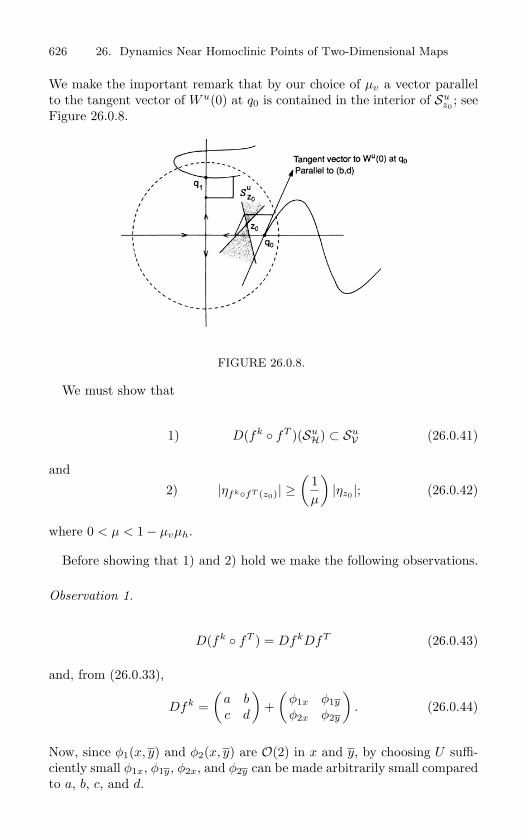
626 26. Dynamics Near Homoclinic Points of Two-Dimensional Maps
We make the important remark that by our choice of µv a vector parallelto the tangent vector of Wu(0) at q0 is contained in the interior of Su
z0; see
Figure 26.0.8.
FIGURE 26.0.8.
We must show that
1) D(fk fT )(SuH) ⊂ Su
V (26.0.41)
and
2) |ηfkfT (z0)| ≥(
1µ
)|ηz0 |; (26.0.42)
where 0 < µ < 1− µvµh.
Before showing that 1) and 2) hold we make the following observations.
Observation 1.
D(fk fT ) = DfkDfT (26.0.43)
and, from (26.0.33),
Dfk =(
a bc d
)+
(φ1x φ1y
φ2x φ2y
). (26.0.44)
Now, since φ1(x, y) and φ2(x, y) are O(2) in x and y, by choosing U suffi-ciently small φ1x, φ1y, φ2x, and φ2y can be made arbitrarily small comparedto a, b, c, and d.
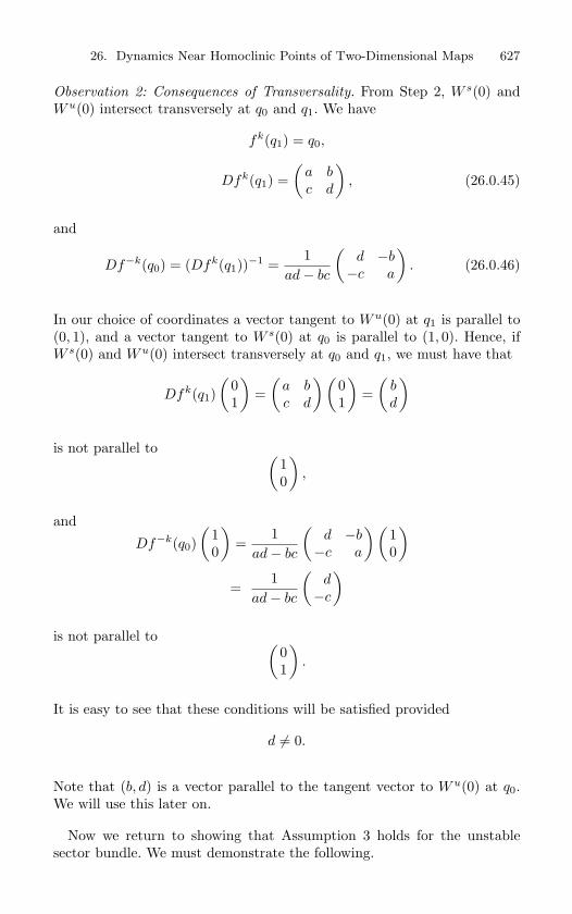
26. Dynamics Near Homoclinic Points of Two-Dimensional Maps 627
Observation 2: Consequences of Transversality. From Step 2, W s(0) andWu(0) intersect transversely at q0 and q1. We have
fk(q1) = q0,
Dfk(q1) =(
a bc d
), (26.0.45)
and
Df−k(q0) = (Dfk(q1))−1 =1
ad− bc
(d −b−c a
). (26.0.46)
In our choice of coordinates a vector tangent to Wu(0) at q1 is parallel to(0, 1), and a vector tangent to W s(0) at q0 is parallel to (1, 0). Hence, ifW s(0) and Wu(0) intersect transversely at q0 and q1, we must have that
Dfk(q1)(
01
)=
(a bc d
)(01
)=
(bd
)
is not parallel to (10
),
and
Df−k(q0)(
10
)=
1ad− bc
(d −b−c a
)(10
)
=1
ad− bc
(d−c
)
is not parallel to (01
).
It is easy to see that these conditions will be satisfied provided
d = 0.
Note that (b, d) is a vector parallel to the tangent vector to Wu(0) at q0.We will use this later on.
Now we return to showing that Assumption 3 holds for the unstablesector bundle. We must demonstrate the following.
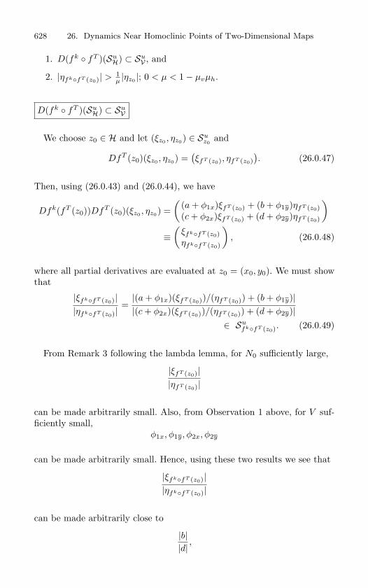
628 26. Dynamics Near Homoclinic Points of Two-Dimensional Maps
1. D(fk fT )(SuH) ⊂ Su
V , and
2. |ηfkfT (z0)| > 1µ |ηz0 |; 0 < µ < 1− µvµh.
D(fk fT )(SuH) ⊂ Su
V
We choose z0 ∈ H and let (ξz0 , ηz0) ∈ Suz0
and
DfT (z0)(ξz0 , ηz0) =(ξfT (z0), ηfT (z0)
). (26.0.47)
Then, using (26.0.43) and (26.0.44), we have
Dfk(fT (z0))DfT (z0)(ξz0 , ηz0) =(
(a + φ1x)ξfT (z0) + (b + φ1y)ηfT (z0)(c + φ2x)ξfT (z0) + (d + φ2y)ηfT (z0)
)
≡(
ξfkfT (z0)ηfkfT (z0)
), (26.0.48)
where all partial derivatives are evaluated at z0 = (x0, y0). We must showthat
|ξfkfT (z0)||ηfkfT (z0)|
=|(a + φ1x)(ξfT (z0))/(ηfT (z0)) + (b + φ1y)||(c + φ2x)(ξfT (z0))/(ηfT (z0)) + (d + φ2y)|
∈ SufkfT (z0). (26.0.49)
From Remark 3 following the lambda lemma, for N0 sufficiently large,
|ξfT (z0)||ηfT (z0)|
can be made arbitrarily small. Also, from Observation 1 above, for V suf-ficiently small,
φ1x, φ1y, φ2x, φ2y
can be made arbitrarily small. Hence, using these two results we see that
|ξfkfT (z0)||ηfkfT (z0)|
can be made arbitrarily close to
|b||d| ,
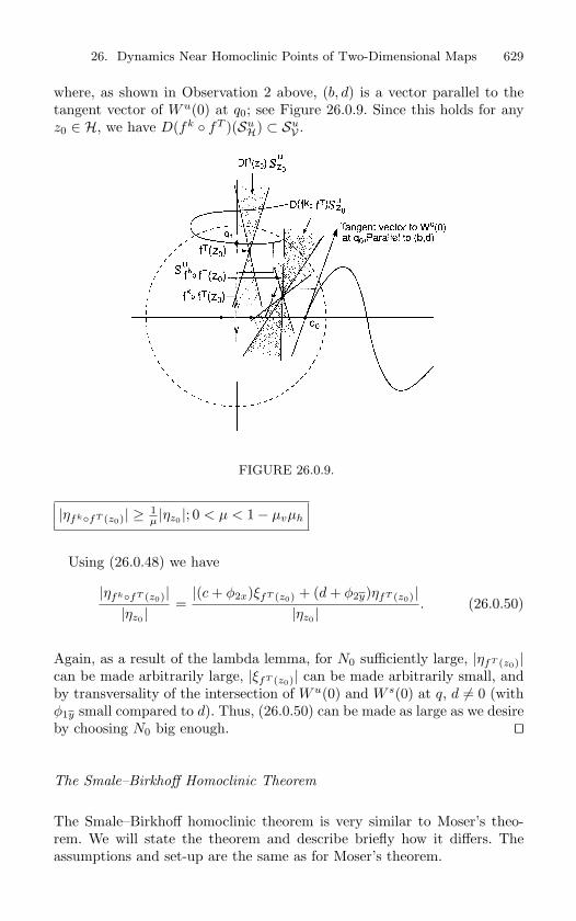
26. Dynamics Near Homoclinic Points of Two-Dimensional Maps 629
where, as shown in Observation 2 above, (b, d) is a vector parallel to thetangent vector of Wu(0) at q0; see Figure 26.0.9. Since this holds for anyz0 ∈ H, we have D(fk fT )(Su
H) ⊂ SuV .
FIGURE 26.0.9.
|ηfkfT (z0)| ≥ 1µ |ηz0 |; 0 < µ < 1− µvµh
Using (26.0.48) we have
|ηfkfT (z0)||ηz0 |
=|(c + φ2x)ξfT (z0) + (d + φ2y)ηfT (z0)|
|ηz0 |. (26.0.50)
Again, as a result of the lambda lemma, for N0 sufficiently large, |ηfT (z0)|can be made arbitrarily large, |ξfT (z0)| can be made arbitrarily small, andby transversality of the intersection of Wu(0) and W s(0) at q, d = 0 (withφ1y small compared to d). Thus, (26.0.50) can be made as large as we desireby choosing N0 big enough.
The Smale–Birkhoff Homoclinic Theorem
The Smale–Birkhoff homoclinic theorem is very similar to Moser’s theo-rem. We will state the theorem and describe briefly how it differs. Theassumptions and set-up are the same as for Moser’s theorem.
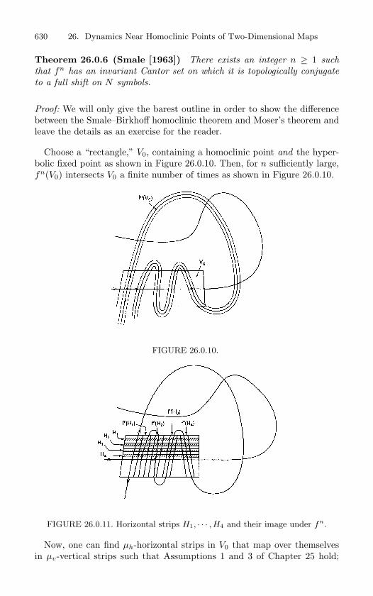
630 26. Dynamics Near Homoclinic Points of Two-Dimensional Maps
Theorem 26.0.6 (Smale [1963]) There exists an integer n ≥ 1 such
that fn has an invariant Cantor set on which it is topologically conjugate
to a full shift on N symbols.
Proof: We will only give the barest outline in order to show the differencebetween the Smale–Birkhoff homoclinic theorem and Moser’s theorem andleave the details as an exercise for the reader.
Choose a “rectangle,” V0, containing a homoclinic point and the hyper-bolic fixed point as shown in Figure 26.0.10. Then, for n sufficiently large,fn(V0) intersects V0 a finite number of times as shown in Figure 26.0.10.
FIGURE 26.0.10.
FIGURE 26.0.11. Horizontal strips H1, · · · , H4 and their image under fn.
Now, one can find µh-horizontal strips in V0 that map over themselvesin µv-vertical strips such that Assumptions 1 and 3 of Chapter 25 hold;
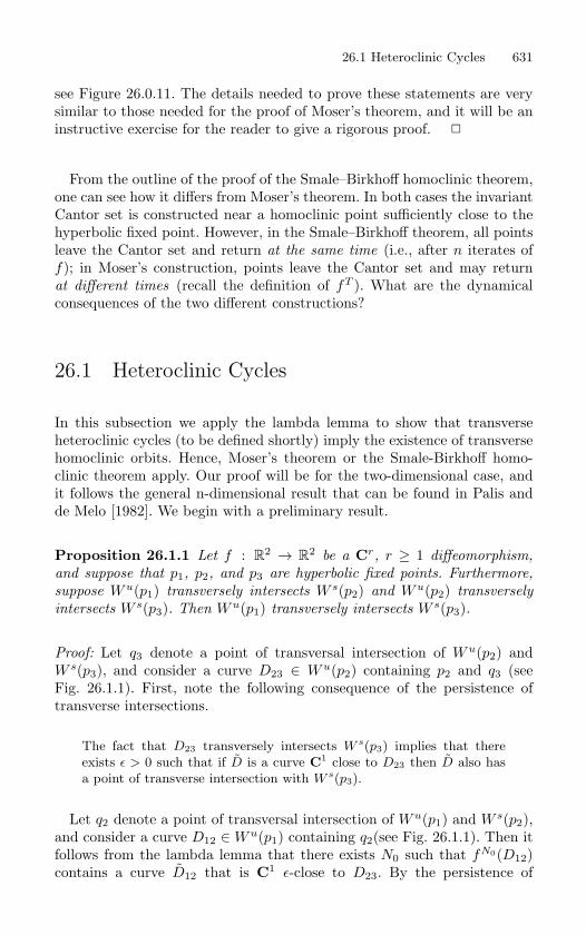
26.1 Heteroclinic Cycles 631
see Figure 26.0.11. The details needed to prove these statements are verysimilar to those needed for the proof of Moser’s theorem, and it will be aninstructive exercise for the reader to give a rigorous proof.
From the outline of the proof of the Smale–Birkhoff homoclinic theorem,one can see how it differs from Moser’s theorem. In both cases the invariantCantor set is constructed near a homoclinic point sufficiently close to thehyperbolic fixed point. However, in the Smale–Birkhoff theorem, all pointsleave the Cantor set and return at the same time (i.e., after n iterates off); in Moser’s construction, points leave the Cantor set and may returnat different times (recall the definition of fT ). What are the dynamicalconsequences of the two different constructions?
26.1 Heteroclinic Cycles
In this subsection we apply the lambda lemma to show that transverseheteroclinic cycles (to be defined shortly) imply the existence of transversehomoclinic orbits. Hence, Moser’s theorem or the Smale-Birkhoff homo-clinic theorem apply. Our proof will be for the two-dimensional case, andit follows the general n-dimensional result that can be found in Palis andde Melo [1982]. We begin with a preliminary result.
Proposition 26.1.1 Let f : R2 → R
2 be a Cr, r ≥ 1 diffeomorphism,
and suppose that p1, p2, and p3 are hyperbolic fixed points. Furthermore,
suppose Wu(p1) transversely intersects W s(p2) and Wu(p2) transversely
intersects W s(p3). Then Wu(p1) transversely intersects W s(p3).
Proof: Let q3 denote a point of transversal intersection of Wu(p2) andW s(p3), and consider a curve D23 ∈ Wu(p2) containing p2 and q3 (seeFig. 26.1.1). First, note the following consequence of the persistence oftransverse intersections.
The fact that D23 transversely intersects W s(p3) implies that there
exists ε > 0 such that if D is a curve C1 close to D23 then D also has
a point of transverse intersection with W s(p3).
Let q2 denote a point of transversal intersection of Wu(p1) and W s(p2),and consider a curve D12 ∈ Wu(p1) containing q2(see Fig. 26.1.1). Then itfollows from the lambda lemma that there exists N0 such that fN0(D12)contains a curve D12 that is C1 ε-close to D23. By the persistence of
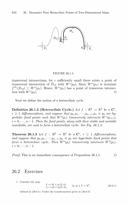
632 26. Dynamics Near Homoclinic Points of Two-Dimensional Maps
2p
1p p3
q
2
3
qD
23
12
D
FIGURE 26.1.1.
transversal intersections, for ε sufficiently small there exists a point oftransversal intersection of D12 with W s(p3). Since Wu(p1) is invariantfN0(D12) ⊂ Wu(p1). Hence, Wu(p1) has a point of transverse intersec-tion with W s(p3).
Next we define the notion of a heteroclinic cycle.
Definition 26.1.2 (Heteroclinic Cycle.) Let f : R2 → R
2 be a Cr,
r ≥ 1 diffeomorphism, and suppose that p0, p1, · · · , pn−1, pn ≡ p0 are hy-
perbolic fixed points such that Wu(pi) transversely intersects W s(pi+1),i = 0, · · · , n− 1. Then the fixed points, along with their stable and unstable
manifolds, are said to form a heteroclinic cycle. See Fig. 26.1.2.
Theorem 26.1.3 Let f : R2 → R
2 be a Cr, r ≥ 1 diffeomorphism,
and suppose that p0, p1, · · · , pn−1, pn ≡ p0 are hyperbolic fixed points that
form a heteroclinic cycle. Then Wu(pi) transversely intersects W s(pi),i = 0, · · · , n− 1.
Proof: This is an immediate consequence of Proposition 26.1.1.
26.2 Exercises
1. Consider the mapξ → λξ + g1(ξ, η),η → µη + g2(ξ, η), (ξ, η) ∈ U ⊂ R
2, (26.2.1)
defined in (26.0.1). Under the transformation given in (26.0.3)
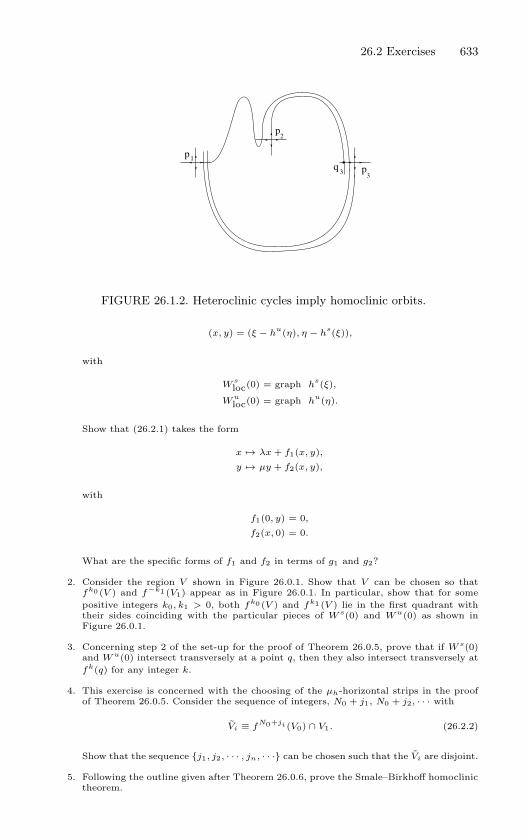
26.2 Exercises 633
2p
1p
p3
q3
FIGURE 26.1.2. Heteroclinic cycles imply homoclinic orbits.
(x, y) = (ξ − hu(η), η − h
s(ξ)),
with
Wsloc(0) = graph h
s(ξ),
Wuloc(0) = graph h
u(η).
Show that (26.2.1) takes the form
x → λx + f1(x, y),
y → µy + f2(x, y),
with
f1(0, y) = 0,
f2(x, 0) = 0.
What are the specific forms of f1 and f2 in terms of g1 and g2?
2. Consider the region V shown in Figure 26.0.1. Show that V can be chosen so thatfk0 (V ) and f−k1 (V1) appear as in Figure 26.0.1. In particular, show that for somepositive integers k0, k1 > 0, both fk0 (V ) and fk1 (V ) lie in the first quadrant withtheir sides coinciding with the particular pieces of W s(0) and W u(0) as shown inFigure 26.0.1.
3. Concerning step 2 of the set-up for the proof of Theorem 26.0.5, prove that if W s(0)and W u(0) intersect transversely at a point q, then they also intersect transversely atfk(q) for any integer k.
4. This exercise is concerned with the choosing of the µh-horizontal strips in the proofof Theorem 26.0.5. Consider the sequence of integers, N0 + j1, N0 + j2, · · · with
Vi ≡ fN0+ji (V0) ∩ V1. (26.2.2)
Show that the sequence j1, j2, · · · , jn, · · · can be chosen such that the Vi are disjoint.
5. Following the outline given after Theorem 26.0.6, prove the Smale–Birkhoff homoclinictheorem.
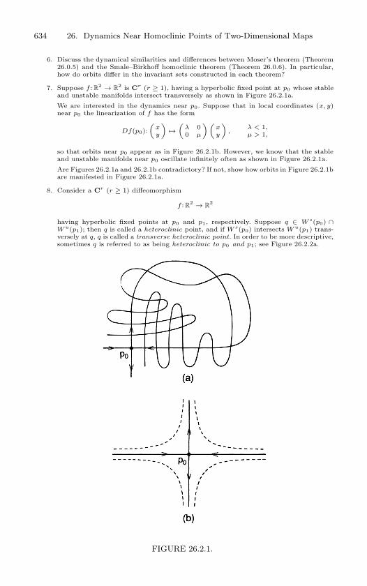
634 26. Dynamics Near Homoclinic Points of Two-Dimensional Maps
6. Discuss the dynamical similarities and differences between Moser’s theorem (Theorem26.0.5) and the Smale–Birkhoff homoclinic theorem (Theorem 26.0.6). In particular,how do orbits differ in the invariant sets constructed in each theorem?
7. Suppose f : R2 → R
2 is Cr (r ≥ 1), having a hyperbolic fixed point at p0 whose stableand unstable manifolds intersect transversely as shown in Figure 26.2.1a.
We are interested in the dynamics near p0. Suppose that in local coordinates (x, y)near p0 the linearization of f has the form
Df(p0):(
xy
)→
(λ 00 µ
)(xy
),
λ < 1,µ > 1,
so that orbits near p0 appear as in Figure 26.2.1b. However, we know that the stableand unstable manifolds near p0 oscillate infinitely often as shown in Figure 26.2.1a.
Are Figures 26.2.1a and 26.2.1b contradictory? If not, show how orbits in Figure 26.2.1bare manifested in Figure 26.2.1a.
8. Consider a Cr (r ≥ 1) diffeomorphism
f : R2 → R
2
having hyperbolic fixed points at p0 and p1, respectively. Suppose q ∈ W s(p0) ∩W u(p1); then q is called a heteroclinic point, and if W s(p0) intersects W u(p1) trans-versely at q, q is called a transverse heteroclinic point. In order to be more descriptive,sometimes q is referred to as being heteroclinic to p0 and p1; see Figure 26.2.2a.
FIGURE 26.2.1.
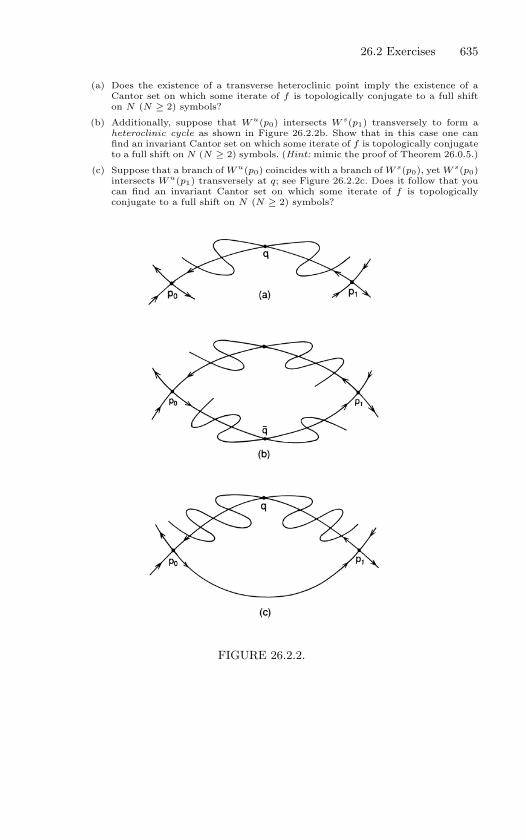
26.2 Exercises 635
(a) Does the existence of a transverse heteroclinic point imply the existence of aCantor set on which some iterate of f is topologically conjugate to a full shifton N (N ≥ 2) symbols?
(b) Additionally, suppose that W u(p0) intersects W s(p1) transversely to form aheteroclinic cycle as shown in Figure 26.2.2b. Show that in this case one canfind an invariant Cantor set on which some iterate of f is topologically conjugateto a full shift on N (N ≥ 2) symbols. (Hint: mimic the proof of Theorem 26.0.5.)
(c) Suppose that a branch of W u(p0) coincides with a branch of W s(p0), yet W s(p0)intersects W u(p1) transversely at q; see Figure 26.2.2c. Does it follow that youcan find an invariant Cantor set on which some iterate of f is topologicallyconjugate to a full shift on N (N ≥ 2) symbols?
FIGURE 26.2.2.
27
Orbits Homoclinic toHyperbolic Fixed Points inThree-DimensionalAutonomous Vector Fields
In this chapter we will study the orbit structure near orbits homoclinicto hyperbolic fixed points of three-dimensional autonomous vector fields.The term “near” refers to both phase space and parameter space. Wewill see that in some cases Smale horseshoe–type behavior may arise. Inparametrized systems the creation of the horseshoes may be accompaniedby cascades of period-doubling and saddle-node bifurcations as described inTheorem 32.1.2, or the horseshoes may “explode” into creation at a criticalparameter value. We will see that the nature of the orbit structure nearthe homoclinic orbits depends mainly on two properties of the vector field:
1. the nature of the eigenvalues of the linearized vector field at the fixedpoint;
2. the existence of multiple homoclinic orbits to the same hyperbolicfixed point which could be a consequence of symmetries of the vectorfield;
3. the global geometry of the stable and unstable manifolds (roughlyspeaking, how they “twist” in phase space).
Regarding Property 1, it should be clear that there are only two possi-bilities for the three eigenvalues associated with the linearized vector field.
1. Saddle λ1, λ2, λ3 real with λ1, λ2 < 0, λ3 > 0.
2. Saddle-focus ρ± iω, λ with ρ < 0, λ > 0.
All other possibilities for hyperbolic fixed points follow from these twovia time reversal. We will analyze each situation individually, but first we
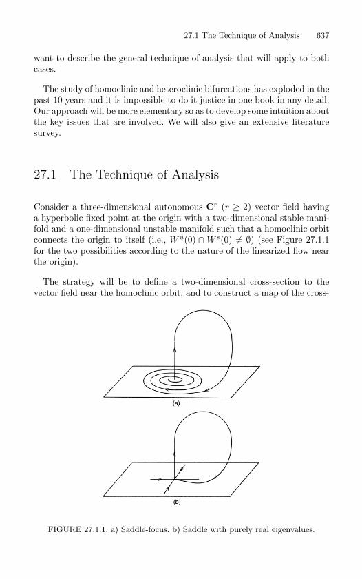
27.1 The Technique of Analysis 637
want to describe the general technique of analysis that will apply to bothcases.
The study of homoclinic and heteroclinic bifurcations has exploded in thepast 10 years and it is impossible to do it justice in one book in any detail.Our approach will be more elementary so as to develop some intuition aboutthe key issues that are involved. We will also give an extensive literaturesurvey.
27.1 The Technique of Analysis
Consider a three-dimensional autonomous Cr (r ≥ 2) vector field havinga hyperbolic fixed point at the origin with a two-dimensional stable mani-fold and a one-dimensional unstable manifold such that a homoclinic orbitconnects the origin to itself (i.e., Wu(0) ∩W s(0) = ∅) (see Figure 27.1.1for the two possibilities according to the nature of the linearized flow nearthe origin).
The strategy will be to define a two-dimensional cross-section to thevector field near the homoclinic orbit, and to construct a map of the cross-
FIGURE 27.1.1. a) Saddle-focus. b) Saddle with purely real eigenvalues.
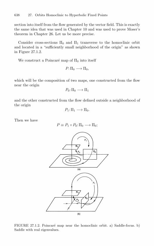
638 27. Orbits Homoclinic to Hyperbolic Fixed Points
section into itself from the flow generated by the vector field. This is exactlythe same idea that was used in Chapter 10 and was used to prove Moser’stheorem in Chapter 26. Let us be more precise.
Consider cross-sections Π0 and Π1 transverse to the homoclinic orbitand located in a “sufficiently small neighborhood of the origin” as shownin Figure 27.1.2.
We construct a Poincare map of Π0 into itself
P : Π0 −→ Π0,
which will be the composition of two maps, one constructed from the flownear the origin
P0: Π0 −→ Π1
and the other constructed from the flow defined outside a neighborhood ofthe origin
P1: Π1 −→ Π0.
Then we haveP ≡ P1 P0: Π0 −→ Π0;
FIGURE 27.1.2. Poincare map near the homoclinic orbit. a) Saddle-focus. b)
Saddle with real eigenvalues.
27.1 The Technique of Analysis 639
see Figure 27.1.2. Thus, the entire construction requires four steps.
Step 1: Define Π0 and Π1. We will do this in each of the cases individu-ally. As is typical, the choice of a cross-section on which to define aPoincare map requires some knowledge of the geometrical structure ofthe phase space. A clever choice can often simplify the computationsconsiderably.
Step 2: Construction of P0. For Π0 and Π1 located sufficiently close to theorigin, the map of Π0 into Π1 is “essentially” given by the flow gen-erated by the linearized vector field. We put “essentially” in quotes,because using the linearized vector field to construct P0 does intro-duce an error. However, the error can be made arbitrarily small bytaking Π0 and Π1 sufficiently small and close to the origin; see Wig-gins [1988] and Bakaleinikov and Silbergleit [1995a], [1995b]. More-over, this error is truly negligible in the sense that it does not affectour results. Therefore, we will construct P0 from the flow generatedby the linearized vector field in order to avoid unnecessary technicaldistractions.
Step 3: Construction of P1. Let p0 ≡ Wu(0) ∩ Π0 and p1 ≡ Wu(0) ∩ Π1.Then the time of flight from p0 to p1 is finite, since we are outside of aneighborhood of the fixed point. We will assume that, except for theorigin, the homoclinic orbit is bounded away from all other possiblefixed points of the vector field. Then, by continuity with respect toinitial conditions, for Π0 sufficiently small, the flow generated by thevector field maps Π0 onto Π1. This implies that the map P1 is definedfor Π0 sufficiently small.
Thus, P0 is defined, but how is it computed? Taylor expanding P1about p0 gives
P1(h) = p0 + DP1(p1)h +O(|h|2),
where h represents coordinates on Π1 centered at p1. Now for Π1sufficiently small the O(|h|2) term in this expression can be madearbitrarily small. Therefore, for P1: Π1 → Π0, we will take
P1(h) = p0 + DP1(p1)h.
Of course, this approximation to P1 introduces an error. However, inWiggins [1988] and Bakaleinikov and Silbergleit [1995a,b] it is shownthat the error is truly negligible in the sense that it does not affectour results. In some cases it will be necessary to assume that DP1(p1)is a diffeomorphism.
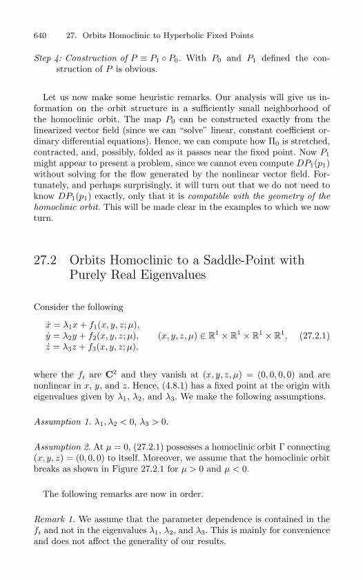
640 27. Orbits Homoclinic to Hyperbolic Fixed Points
Step 4: Construction of P ≡ P1 P0. With P0 and P1 defined the con-struction of P is obvious.
Let us now make some heuristic remarks. Our analysis will give us in-formation on the orbit structure in a sufficiently small neighborhood ofthe homoclinic orbit. The map P0 can be constructed exactly from thelinearized vector field (since we can “solve” linear, constant coefficient or-dinary differential equations). Hence, we can compute how Π0 is stretched,contracted, and, possibly, folded as it passes near the fixed point. Now P1might appear to present a problem, since we cannot even compute DP1(p1)without solving for the flow generated by the nonlinear vector field. For-tunately, and perhaps surprisingly, it will turn out that we do not need toknow DP1(p1) exactly, only that it is compatible with the geometry of the
homoclinic orbit. This will be made clear in the examples to which we nowturn.
27.2 Orbits Homoclinic to a Saddle-Point withPurely Real Eigenvalues
Consider the following
x = λ1x + f1(x, y, z;µ),y = λ2y + f2(x, y, z;µ),z = λ3z + f3(x, y, z; µ),
(x, y, z, µ) ∈ R1 × R
1 × R1 × R
1, (27.2.1)
where the fi are C2 and they vanish at (x, y, z, µ) = (0, 0, 0, 0) and arenonlinear in x, y, and z. Hence, (4.8.1) has a fixed point at the origin witheigenvalues given by λ1, λ2, and λ3. We make the following assumptions.
Assumption 1. λ1, λ2 < 0, λ3 > 0.
Assumption 2. At µ = 0, (27.2.1) possesses a homoclinic orbit Γ connecting(x, y, z) = (0, 0, 0) to itself. Moreover, we assume that the homoclinic orbitbreaks as shown in Figure 27.2.1 for µ > 0 and µ < 0.
The following remarks are now in order.
Remark 1. We assume that the parameter dependence is contained in thefi and not in the eigenvalues λ1, λ2, and λ3. This is mainly for convenienceand does not affect the generality of our results.
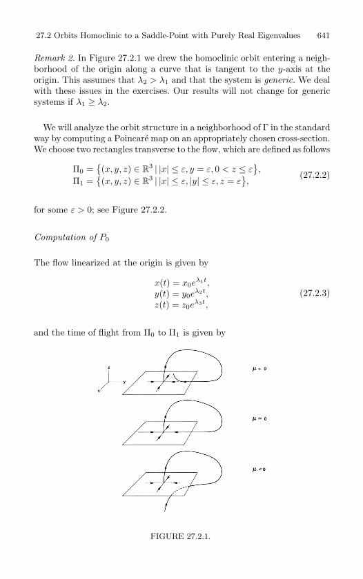
27.2 Orbits Homoclinic to a Saddle-Point with Purely Real Eigenvalues 641
Remark 2. In Figure 27.2.1 we drew the homoclinic orbit entering a neigh-borhood of the origin along a curve that is tangent to the y-axis at theorigin. This assumes that λ2 > λ1 and that the system is generic. We dealwith these issues in the exercises. Our results will not change for genericsystems if λ1 ≥ λ2.
We will analyze the orbit structure in a neighborhood of Γ in the standardway by computing a Poincare map on an appropriately chosen cross-section.We choose two rectangles transverse to the flow, which are defined as follows
Π0 =(x, y, z) ∈ R
3 | |x| ≤ ε, y = ε, 0 < z ≤ ε,
Π1 =(x, y, z) ∈ R
3 | |x| ≤ ε, |y| ≤ ε, z = ε,
(27.2.2)
for some ε > 0; see Figure 27.2.2.
Computation of P0
The flow linearized at the origin is given by
x(t) = x0eλ1t,
y(t) = y0eλ2t,
z(t) = z0eλ3t,
(27.2.3)
and the time of flight from Π0 to Π1 is given by
FIGURE 27.2.1.
642 27. Orbits Homoclinic to Hyperbolic Fixed Points
t =1λ3
logε
z0. (27.2.4)
Hence, the mapP0: Π0 → Π1
is given by (leaving off the subscript 0’s)
x
εz
→
x
(εz
)λ1/λ3
ε(
εz
)λ2/λ3
ε
. (27.2.5)
Computation of P1
Following the discussion of Step 3 in our general analysis above, we takeas P1 the following affine map
P1: Π1 −→ Π0x
yε
→
0
ε0
+
a b 0
0 0 0c d 0
x
y0
+
eµ
0fµ
, (27.2.6)
where a, b, c, d, e, and f are constants. Note from Figure 27.2.1 that wehave f > 0, so we may rescale the parameter µ so that f = 1. Henceforth,we will assume that this has been done. Let us briefly explain the form of(27.2.6). On Π0 the y coordinate is fixed at y = ε. This explains why thereare only zeros in the middle row of the linear part of (27.2.6). Also, the zcoordinate of Π1 is fixed at z = ε. This explains why there are only zerosin the third column of the matrix in (27.2.6).
FIGURE 27.2.2.
27.2 Orbits Homoclinic to a Saddle-Point with Purely Real Eigenvalues 643
The Poincare Map P ≡ P1 P0
Forming the composition of P0 and P1, we obtain the Poincare map definedin a neighborhood of the homoclinic orbit having the following form.
P ≡ P1 P0: Π0 → Π0,(xz
)→
(ax
(εz
)λ1/λ3 + bε(
εz
)λ2/λ3 + eµ
cx(
εz
)λ1/λ3 + dε(
εz
)λ2/λ3 + µ
), (27.2.7)
where Π0 is chosen sufficiently small so that P1 P0 is defined.
We reiterate that the approximate Poincare map (27.2.7) is valid for εsufficiently small and x and z sufficiently small. For ε sufficiently small,the approximation of P0 by the linearized flow is valid and, for x and zsufficiently small, the approximation of P1 by the affine map P1 is valid.Note that ε, x, and z are independent.
Calculation of Fixed Points of P
Now we look for fixed points of the Poincare map (which will correspondto periodic orbits of (27.2.1). First some notation; let
A = aελ1/λ3 , B = bε1+(λ2/λ3), C = cελ1/λ3 , D = dε1+(λ2/λ3).
Then the condition for fixed points of (27.2.7) is
x = Axz|λ1|/λ3 + Bz|λ2|/λ3 + eµ, (27.2.8)
z = Cxz|λ1|/λ3 + Dz|λ2|/λ3 + µ. (27.2.9)
Solving (27.2.8) for x as a function of z gives
x =Bz|λ2|/λ3 + eµ
1−Az|λ1|/λ3. (27.2.10)
We will restrict ourselves to a sufficiently small neighborhood of thehomoclinic orbit so that z can be taken sufficiently small in order that thedenominator of (27.2.10) can be taken to be 1. Substituting this expressionfor x into (27.2.9) gives the following condition for fixed points of (27.2.7)in terms of z and µ only
z − µ = CBz|λ1+λ2|/λ3 + Ceµz|λ1|/λ3 + Dz|λ2|/λ3 . (27.2.11)
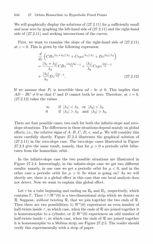
644 27. Orbits Homoclinic to Hyperbolic Fixed Points
We will graphically display the solutions of (27.2.11) for µ sufficiently smalland near zero by graphing the left-hand side of (27.2.11) and the right-handside of (27.2.11) and seeking intersections of the curves.
First, we want to examine the slope of the right-hand side of (27.2.11)at z = 0. This is given by the following expression
d
dz
(CBz|λ1+λ2|/λ3 + Ceµz|λ1|/λ3 + Dz|λ2|/λ3
)=|λ1 + λ2|
λ3CBz
|λ1+λ2|λ3
−1 +|λ1|λ3
Ceµz|λ1|λ3
−1
+|λ2|λ3
Dz|λ2|λ3
−1. (27.2.12)
If we assume that P1 is invertible then ad − bc = 0. This implies thatAD −BC = 0 so that C and D cannot both be zero. Therefore, at z = 0,(27.2.12) takes the values
∞ if |λ1| < λ3 or |λ2| < λ30 if |λ1| > λ3 and |λ2| > λ3.
There are four possible cases, two each for both the infinite-slope and zero-slope situations. The differences in these situations depend mainly on globaleffects, i.e., the relative signs of A, B, C, D, e, and µ. We will consider thismore carefully shortly. Figure 27.2.3 illustrates the graphical solution of(27.2.11) in the zero-slope case. The two-slope cases illustrated in Figure27.2.3 give the same result, namely, that for µ > 0 a periodic orbit bifur-cates from the homoclinic orbit.
In the infinite-slope case the two possible situations are illustrated inFigure 27.2.4. Interestingly, in the infinite-slope case we get two differentresults; namely, in one case we get a periodic orbit for µ < 0, and in theother case a periodic orbit for µ > 0. So what is going on? As we willshortly see, there is a global effect in this case that our local analysis doesnot detect. Now we want to explain this global effect.
Let τ be a tube beginning and ending on Π0 and Π1, respectively, whichcontains Γ. Then τ ∩W s(0) is a two-dimensional strip which we denote asR. Suppose, without twisting R, that we join together the two ends of R.Then there are two possibilities: 1) W s(0) experiences an even number ofhalf-twists inside τ , in which case, when the ends of R are joined together itis homeomorphic to a cylinder, or 2) W s(0) experiences an odd number ofhalf-twists inside τ , in which case, when the ends of R are joined togetherit is homeomorphic to a Mobius strip; see Figure 27.2.5. The reader shouldverify this experimentally with a strip of paper.
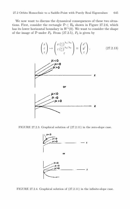
27.2 Orbits Homoclinic to a Saddle-Point with Purely Real Eigenvalues 645
We now want to discuss the dynamical consequences of these two situa-tions. First, consider the rectangle D ⊂ Π0 shown in Figure 27.2.6, whichhas its lower horizontal boundary in W s(0). We want to consider the shapeof the image of D under P0. From (27.2.5), P0 is given by
x
εz
→
x
(εz
)λ1/λ3
ε(
εz
)λ2/λ3
ε
≡
x′
y′
ε
, (27.2.13)
FIGURE 27.2.3. Graphical solution of (27.2.11) in the zero-slope case.
FIGURE 27.2.4. Graphical solution of (27.2.11) in the infinite-slope case.
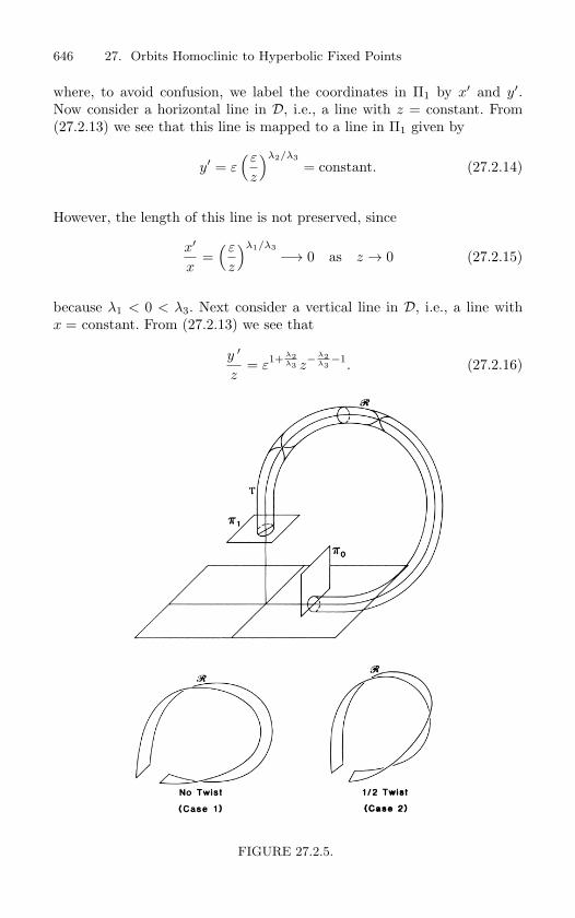
646 27. Orbits Homoclinic to Hyperbolic Fixed Points
where, to avoid confusion, we label the coordinates in Π1 by x′ and y′.Now consider a horizontal line in D, i.e., a line with z = constant. From(27.2.13) we see that this line is mapped to a line in Π1 given by
y′ = ε( ε
z
)λ2/λ3
= constant. (27.2.14)
However, the length of this line is not preserved, since
x′
x=
( ε
z
)λ1/λ3
−→ 0 as z → 0 (27.2.15)
because λ1 < 0 < λ3. Next consider a vertical line in D, i.e., a line withx = constant. From (27.2.13) we see that
y ′
z= ε1+ λ2
λ3 z− λ2λ3
−1. (27.2.16)
FIGURE 27.2.5.
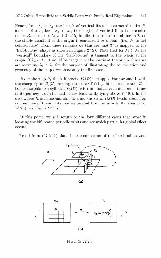
27.2 Orbits Homoclinic to a Saddle-Point with Purely Real Eigenvalues 647
Hence, for −λ2 > λ3, the length of vertical lines is contracted under P0as z → 0 and, for −λ2 < λ3, the length of vertical lines is expandedunder P0 as z → 0. Now, (27.2.15) implies that a horizontal line in D onthe stable manifold of the origin is contracted to a point (i.e., P0 is notdefined here). From these remarks we thus see that D is mapped to the“half-bowtie” shape as shown in Figure 27.2.6. Note that for λ2 > λ1 the“vertical” boundary of the “half-bowtie” is tangent to the y-axis at theorigin. If λ2 < λ1, it would be tangent to the x-axis at the origin. Since weare assuming λ2 > λ1 for the purpose of illustrating the construction andgeometry of the maps, we show only the first case.
Under the map P1 the half-bowtie P0(D) is mapped back around Γ withthe sharp tip of P0(D) coming back near Γ ∩ Π0. In the case where R ishomeomorphic to a cylinder, P0(D) twists around an even number of timesin its journey around Γ and comes back to Π0 lying above W s(0). In thecase where R is homeomorphic to a mobius strip, P0(D) twists around anodd number of times in its journey around Γ and returns to Π0 lying belowW s(0); see Figure 27.2.7.
At this point, we will return to the four different cases that arose inlocating the bifurcated periodic orbits and see which particular global effectoccurs.
Recall from (27.2.11) that the z components of the fixed points were
FIGURE 27.2.6.
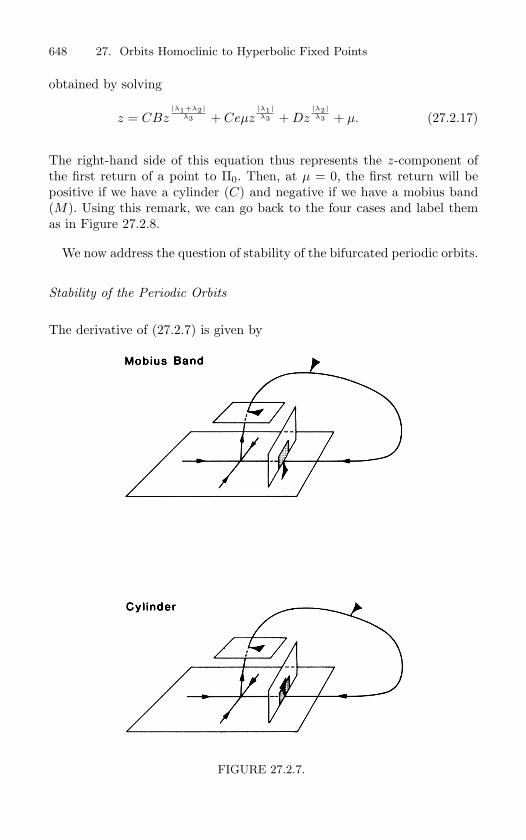
648 27. Orbits Homoclinic to Hyperbolic Fixed Points
obtained by solving
z = CBz|λ1+λ2|
λ3 + Ceµz|λ1|λ3 + Dz
|λ2|λ3 + µ. (27.2.17)
The right-hand side of this equation thus represents the z-component ofthe first return of a point to Π0. Then, at µ = 0, the first return will bepositive if we have a cylinder (C) and negative if we have a mobius band(M). Using this remark, we can go back to the four cases and label themas in Figure 27.2.8.
We now address the question of stability of the bifurcated periodic orbits.
Stability of the Periodic Orbits
The derivative of (27.2.7) is given by
FIGURE 27.2.7.
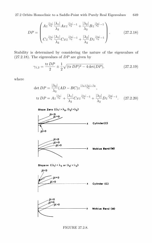
27.2 Orbits Homoclinic to a Saddle-Point with Purely Real Eigenvalues 649
DP =
Az|λ1|λ3|λ1|λ3
Axz|λ1|λ3
−1 +|λ2|λ3
Bz|λ2|λ3
−1
Cz|λ1|λ3|λ1|λ3
Cxz|λ1|λ3
−1 +|λ2|λ3
Dz|λ2|λ3
−1
. (27.2.18)
Stability is determined by considering the nature of the eigenvalues of(27.2.18). The eigenvalues of DP are given by
γ1,2 =trDP
2± 1
2
√(trDP )2 − 4 det(DP ), (27.2.19)
where
det DP =|λ2|λ3
(AD −BC)z|λ1+λ2|−λ3
λ3 ,
trDP = Az|λ1|λ3 +
|λ1|λ3
Cxz|λ1|λ3
−1 +|λ2|λ3
Dz|λ2|λ3
−1. (27.2.20)
FIGURE 27.2.8.
650 27. Orbits Homoclinic to Hyperbolic Fixed Points
Substituting equation (27.2.10) for x at a fixed point into the expressionfor trDP gives
trDP = Az|λ1|λ3 +
|λ1|λ3
CBz|λ1+λ2|
λ3−1 +
|λ2|λ3
Dz|λ2|λ3
−1 +|λ1|λ3
Ceµz|λ1|λ3
−1.
(27.2.21)
Let us note the following important facts.
For z sufficiently small
det DP is
a) arbitrarily large for |λ1 + λ2| < λ3;b) arbitrarily small for |λ1 + λ2| > λ3.
trDP is
a) arbitrarily large for |λ1| < λ3 or |λ2| < λ3;b) arbitrarily small for |λ1| > λ3 and |λ2| > λ3.
Using these facts along with (27.2.19) and (27.2.20) we can conclude thefollowing.
1. For |λ1| > λ3 and |λ2| > λ3, both eigenvalues of DP can be madearbitrarily small by taking z sufficiently small.
2. For |λ1 + λ2| > λ3 and |λ1| < λ3 and/or |λ2| < λ3, one eigenvaluecan be made arbitrarily small and the other eigenvalue can be madearbitrarily large by taking z sufficiently small.
3. For |λ1 + λ2| < λ3, either both eigenvalues can be made arbitrarilylarge, or one eigenvalue can be made arbitrarily large and the otherarbitrarily small, by taking z sufficiently small.
We summarize our results in the following theorem.
Theorem 27.2.1 For µ = 0 and sufficiently small, a periodic orbit bifur-
cates from Γ in (27.2.1). The periodic orbit is a
i) sink for |λ1| > λ3 and |λ2| > λ3;
ii) saddle for |λ1 + λ2| > λ3, |λ1| < λ3, and/or |λ2| < λ3;
iii) saddle or source for |λ1 + λ2| < λ3.
We remark that the construction of the Poincare map used in the proofof Theorem 27.2.1 was for the case λ2 > λ1 (see Figure 27.2.1); however,
27.2 Orbits Homoclinic to a Saddle-Point with Purely Real Eigenvalues 651
the same result holds for λ2 < λ1 and λ1 = λ2. We leave the details to thereader in the exercises.
Next we consider the case of two homoclinic orbits connecting the saddletype fixed point to itself and show how under certain conditions chaoticdynamics may arise.
27.2a Two Orbits Homoclinic to a Fixed PointHaving Real Eigenvalues
We consider the same system as before; however, we now replace Assump-tion 2 with Assumption 2′ given below.
Assumption 2 ′. Equation (27.2.1) has a pair of orbits, Γr, Γ, homoclinicto (0, 0, 0) at µ = 0, and Γr and Γ lie in separate branches of the unstablemanifold of (0, 0, 0). There are thus two possible generic pictures illustratedin Figure 27.2.9.
Note that the coordinate axes in Figure 27.2.9 have been rotated withrespect to those in Figure 27.2.1. This is merely for artistic convenience. Wewill consider only the configuration of Case a in Figure 27.2.9; however, thesame analysis (and most of the resulting dynamics) will go through for Caseb. Our goal will be to establish that the Poincare map constructed near thehomoclinic orbits contains the chaotic dynamics of the Smale horseshoe or,more specifically, that it contains an invariant Cantor set on which it ishomeomorphic to the full shift on two symbols (see Chapter 24).
We begin by constructing the local cross-sections to the vector field nearthe origin. We define
Πr0 =
(x, y, z) ∈ R
3 | y = ε, |x| ≤ ε, 0 < z ≤ ε,
Π0 =
(x, y, z) ∈ R
3 | y = ε, |x| ≤ ε, −ε ≤ z < 0,
Πr1 =
(x, y, z) ∈ R
3 | z = ε, |x| ≤ ε, 0 < y ≤ ε,
Π1 =
(x, y, z) ∈ R
3 | z = −ε, |x| ≤ ε, 0 < y ≤ ε,
(27.2.22)
for ε > 0 and small; see Figure 27.2.10 for an illustration of the geometrynear the origin.
Now recall the global twisting of the stable manifold of the origin. Wewant to consider the effect of this in our construction of the Poincare map.Let τr (resp. τ) be a tube beginning and ending on Πr
1 (resp. Π1) and Πr
0(resp. Π
0) which contains Γr (resp. Γ) (see Figure 27.2.5). Then τr∩W s(0)
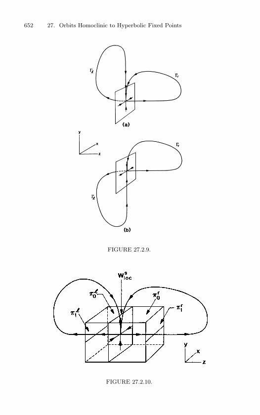
652 27. Orbits Homoclinic to Hyperbolic Fixed Points
FIGURE 27.2.9.
FIGURE 27.2.10.
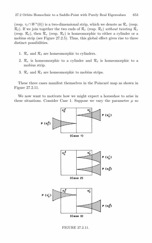
27.2 Orbits Homoclinic to a Saddle-Point with Purely Real Eigenvalues 653
(resp. τ∩W s(0)) is a two-dimensional strip, which we denote as Rr (resp.R). If we join together the two ends of Rr (resp. R) without twisting Rr
(resp. R), then Rr (resp. R) is homeomorphic to either a cylinder or amobius strip (see Figure 27.2.5). Thus, this global effect gives rise to threedistinct possibilities.
1. Rr and R are homeomorphic to cylinders.
2. Rr is homeomorphic to a cylinder and R is homeomorphic to amobius strip.
3. Rr and R are homeomorphic to mobius strips.
These three cases manifest themselves in the Poincare map as shown inFigure 27.2.11.
We now want to motivate how we might expect a horseshoe to arise inthese situations. Consider Case 1. Suppose we vary the parameter µ so
FIGURE 27.2.11.
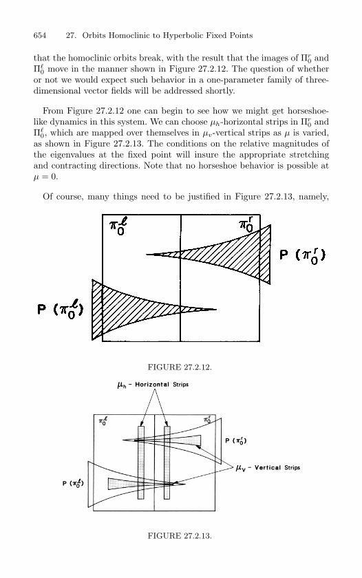
654 27. Orbits Homoclinic to Hyperbolic Fixed Points
that the homoclinic orbits break, with the result that the images of Πr0 and
Π0 move in the manner shown in Figure 27.2.12. The question of whether
or not we would expect such behavior in a one-parameter family of three-dimensional vector fields will be addressed shortly.
From Figure 27.2.12 one can begin to see how we might get horseshoe-like dynamics in this system. We can choose µh-horizontal strips in Πr
0 andΠ
0, which are mapped over themselves in µv-vertical strips as µ is varied,as shown in Figure 27.2.13. The conditions on the relative magnitudes ofthe eigenvalues at the fixed point will insure the appropriate stretchingand contracting directions. Note that no horseshoe behavior is possible atµ = 0.
Of course, many things need to be justified in Figure 27.2.13, namely,
FIGURE 27.2.12.
FIGURE 27.2.13.
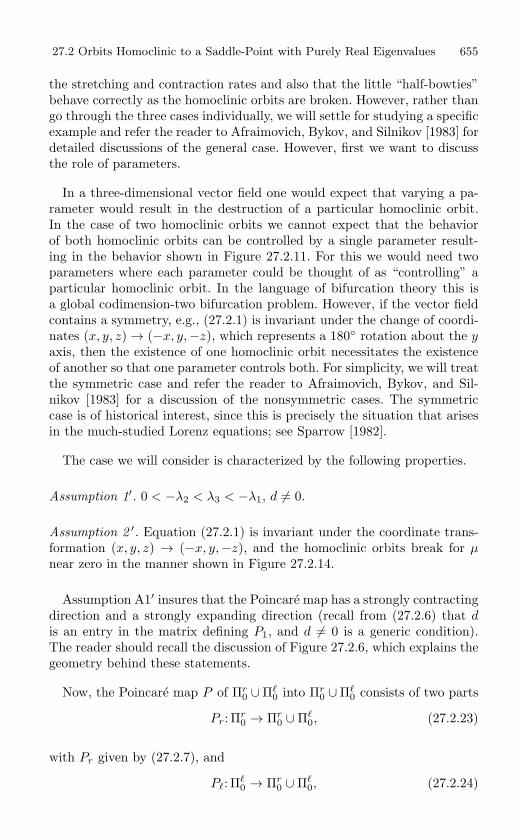
27.2 Orbits Homoclinic to a Saddle-Point with Purely Real Eigenvalues 655
the stretching and contraction rates and also that the little “half-bowties”behave correctly as the homoclinic orbits are broken. However, rather thango through the three cases individually, we will settle for studying a specificexample and refer the reader to Afraimovich, Bykov, and Silnikov [1983] fordetailed discussions of the general case. However, first we want to discussthe role of parameters.
In a three-dimensional vector field one would expect that varying a pa-rameter would result in the destruction of a particular homoclinic orbit.In the case of two homoclinic orbits we cannot expect that the behaviorof both homoclinic orbits can be controlled by a single parameter result-ing in the behavior shown in Figure 27.2.11. For this we would need twoparameters where each parameter could be thought of as “controlling” aparticular homoclinic orbit. In the language of bifurcation theory this isa global codimension-two bifurcation problem. However, if the vector fieldcontains a symmetry, e.g., (27.2.1) is invariant under the change of coordi-nates (x, y, z) → (−x, y,−z), which represents a 180 rotation about the yaxis, then the existence of one homoclinic orbit necessitates the existenceof another so that one parameter controls both. For simplicity, we will treatthe symmetric case and refer the reader to Afraimovich, Bykov, and Sil-nikov [1983] for a discussion of the nonsymmetric cases. The symmetriccase is of historical interest, since this is precisely the situation that arisesin the much-studied Lorenz equations; see Sparrow [1982].
The case we will consider is characterized by the following properties.
Assumption 1′. 0 < −λ2 < λ3 < −λ1, d = 0.
Assumption 2 ′. Equation (27.2.1) is invariant under the coordinate trans-formation (x, y, z) → (−x, y,−z), and the homoclinic orbits break for µnear zero in the manner shown in Figure 27.2.14.
Assumption A1′ insures that the Poincare map has a strongly contractingdirection and a strongly expanding direction (recall from (27.2.6) that dis an entry in the matrix defining P1, and d = 0 is a generic condition).The reader should recall the discussion of Figure 27.2.6, which explains thegeometry behind these statements.
Now, the Poincare map P of Πr0 ∪Π
0 into Πr0 ∪Π
0 consists of two parts
Pr: Πr0 → Πr
0 ∪Π0, (27.2.23)
with Pr given by (27.2.7), and
P: Π0 → Πr
0 ∪Π0, (27.2.24)
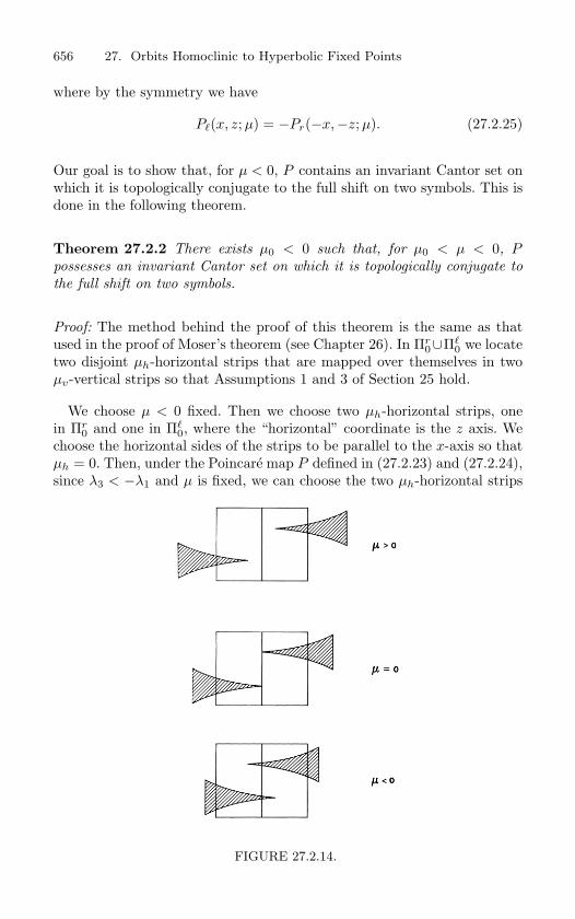
656 27. Orbits Homoclinic to Hyperbolic Fixed Points
where by the symmetry we have
P(x, z;µ) = −Pr(−x,−z;µ). (27.2.25)
Our goal is to show that, for µ < 0, P contains an invariant Cantor set onwhich it is topologically conjugate to the full shift on two symbols. This isdone in the following theorem.
Theorem 27.2.2 There exists µ0 < 0 such that, for µ0 < µ < 0, Ppossesses an invariant Cantor set on which it is topologically conjugate to
the full shift on two symbols.
Proof: The method behind the proof of this theorem is the same as thatused in the proof of Moser’s theorem (see Chapter 26). In Πr
0∪Π0 we locate
two disjoint µh-horizontal strips that are mapped over themselves in twoµv-vertical strips so that Assumptions 1 and 3 of Section 25 hold.
We choose µ < 0 fixed. Then we choose two µh-horizontal strips, onein Πr
0 and one in Π0, where the “horizontal” coordinate is the z axis. We
choose the horizontal sides of the strips to be parallel to the x-axis so thatµh = 0. Then, under the Poincare map P defined in (27.2.23) and (27.2.24),since λ3 < −λ1 and µ is fixed, we can choose the two µh-horizontal strips
FIGURE 27.2.14.
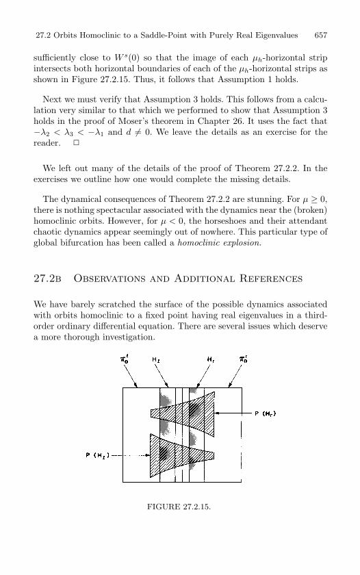
27.2 Orbits Homoclinic to a Saddle-Point with Purely Real Eigenvalues 657
sufficiently close to W s(0) so that the image of each µh-horizontal stripintersects both horizontal boundaries of each of the µh-horizontal strips asshown in Figure 27.2.15. Thus, it follows that Assumption 1 holds.
Next we must verify that Assumption 3 holds. This follows from a calcu-lation very similar to that which we performed to show that Assumption 3holds in the proof of Moser’s theorem in Chapter 26. It uses the fact that−λ2 < λ3 < −λ1 and d = 0. We leave the details as an exercise for thereader.
We left out many of the details of the proof of Theorem 27.2.2. In theexercises we outline how one would complete the missing details.
The dynamical consequences of Theorem 27.2.2 are stunning. For µ ≥ 0,there is nothing spectacular associated with the dynamics near the (broken)homoclinic orbits. However, for µ < 0, the horseshoes and their attendantchaotic dynamics appear seemingly out of nowhere. This particular type ofglobal bifurcation has been called a homoclinic explosion.
27.2b Observations and Additional References
We have barely scratched the surface of the possible dynamics associatedwith orbits homoclinic to a fixed point having real eigenvalues in a third-order ordinary differential equation. There are several issues which deservea more thorough investigation.
FIGURE 27.2.15.
658 27. Orbits Homoclinic to Hyperbolic Fixed Points
1. Two Homoclinic Orbits without Symmetry. See Afraimovich, Bykov,and Silnikov [1983] and the references therein.
2. The Existence of Strange Attractors. Horseshoes are chaotic invari-ant sets, yet all the orbits in the horseshoes are unstable of saddletype. Nevertheless, it should be clear that horseshoes may exhibit astriking effect on the dynamics of any system. In particular, they areoften the chaotic heart of numerically observed strange attractors.For work on the “strange attractor problem” associated with orbitshomoclinic to fixed points having real eigenvalues in a third-orderordinary differential equation, see Afraimovich, Bykov, and Silnikov[1983] and Shashkov and Shil’nikov [1994]. Most of the work done onsuch systems has been in the context of the Lorenz equations. Refer-ences for Lorenz attractors include Sparrow [1982], Guckenheimer andWilliams [1980], and Williams [1980]. Recently, some breakthroughshave been made in proving the existence of strange attractors in suchequations by Rychlik [1990] and Robinson [1989]. Recently, an elegantcomputer assisted proof of the existence of a strange attractor for theLorenz equations was given by Tucker [1999]; see also Morales et al.[1998] and the popular articles of Stewart [2000] and Viana [2000].
3. Bifurcations Creating the Horseshoe. In the homoclinic explosion aninfinite number of periodic orbits of all possible periods are created.The question arises concerning precisely how these periodic orbitswere created and how they are related to each other. This ques-tion also has relevance to the strange attractor problem. See Robin-son [2000], Gonchenko et al. [1996], [1997], and Silnikov and Turaev[1997].
In recent years Birman, Williams, and Holmes have been using theknot type of a periodic orbit as a bifurcation invariant in order tounderstand the appearance, disappearance, and interrelation of pe-riodic orbits in third-order ordinary differential equations. Roughlyspeaking, a periodic orbit in three dimensions can be thought of asa knotted closed loop. As system parameters are varied, the periodicorbit may never intersect itself due to uniqueness of solutions. Hence,the knot type of a periodic orbit cannot change as parameters arevaried. The knot type is therefore a bifurcation invariant as well as akey tool for developing a classification scheme for periodic orbits. Forreferences, see Birman and Williams [1983a,b], Holmes [1986], [1987],Holmes and Williams [1985], Ghrist et al. [1997], Gilmore [1998], andPlumecoq and Lefranc [2000a,b].
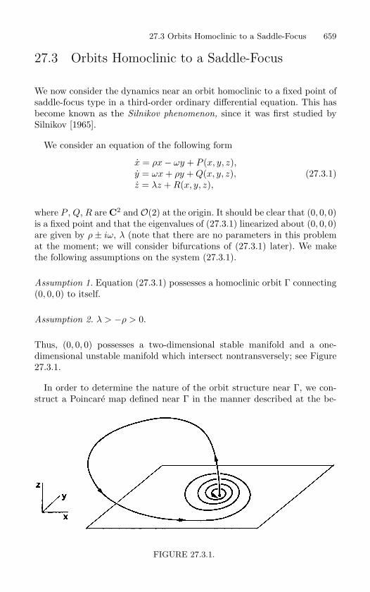
27.3 Orbits Homoclinic to a Saddle-Focus 659
27.3 Orbits Homoclinic to a Saddle-Focus
We now consider the dynamics near an orbit homoclinic to a fixed point ofsaddle-focus type in a third-order ordinary differential equation. This hasbecome known as the Silnikov phenomenon, since it was first studied bySilnikov [1965].
We consider an equation of the following form
x = ρx− ωy + P (x, y, z),y = ωx + ρy + Q(x, y, z),z = λz + R(x, y, z),
(27.3.1)
where P , Q, R are C2 and O(2) at the origin. It should be clear that (0, 0, 0)is a fixed point and that the eigenvalues of (27.3.1) linearized about (0, 0, 0)are given by ρ± iω, λ (note that there are no parameters in this problemat the moment; we will consider bifurcations of (27.3.1) later). We makethe following assumptions on the system (27.3.1).
Assumption 1. Equation (27.3.1) possesses a homoclinic orbit Γ connecting(0, 0, 0) to itself.
Assumption 2. λ > −ρ > 0.
Thus, (0, 0, 0) possesses a two-dimensional stable manifold and a one-dimensional unstable manifold which intersect nontransversely; see Figure27.3.1.
In order to determine the nature of the orbit structure near Γ, we con-struct a Poincare map defined near Γ in the manner described at the be-
FIGURE 27.3.1.
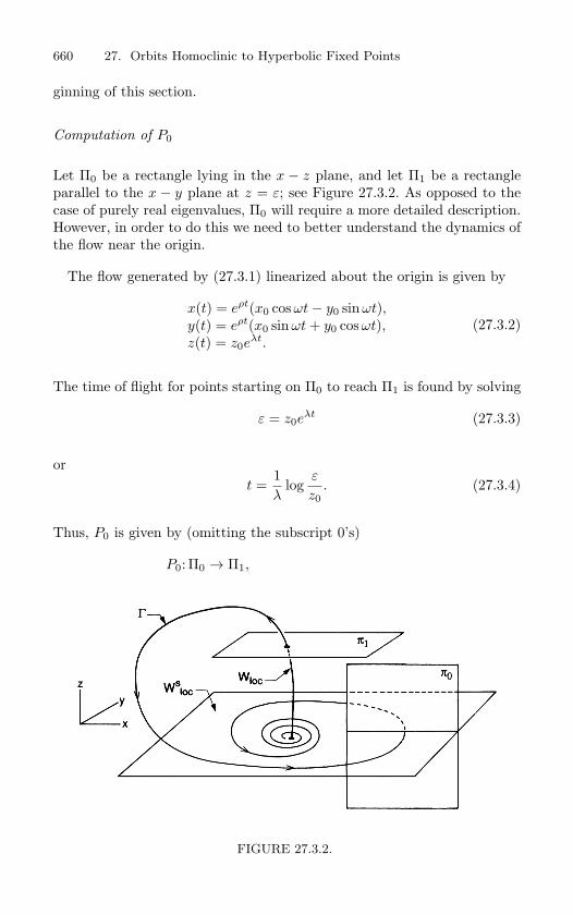
660 27. Orbits Homoclinic to Hyperbolic Fixed Points
ginning of this section.
Computation of P0
Let Π0 be a rectangle lying in the x − z plane, and let Π1 be a rectangleparallel to the x − y plane at z = ε; see Figure 27.3.2. As opposed to thecase of purely real eigenvalues, Π0 will require a more detailed description.However, in order to do this we need to better understand the dynamics ofthe flow near the origin.
The flow generated by (27.3.1) linearized about the origin is given by
x(t) = eρt(x0 cos ωt− y0 sinωt),y(t) = eρt(x0 sinωt + y0 cos ωt),z(t) = z0e
λt.(27.3.2)
The time of flight for points starting on Π0 to reach Π1 is found by solving
ε = z0eλt (27.3.3)
ort =
1λ
logε
z0. (27.3.4)
Thus, P0 is given by (omitting the subscript 0’s)
P0: Π0 → Π1,
FIGURE 27.3.2.
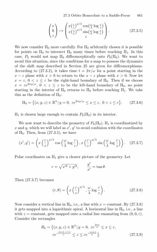
27.3 Orbits Homoclinic to a Saddle-Focus 661
x
0z
→
x
(εz
)ρ/λ cos(
ωλ log ε
z
)x(
εz
)ρ/λ sin(
ωλ log ε
z
)ε
. (27.3.5)
We now consider Π0 more carefully. For Π0 arbitrarily chosen it is possiblefor points on Π0 to intersect Π0 many times before reaching Π1. In thiscase, P0 would not map Π0 diffeomorphically onto P0(Π0). We want toavoid this situation, since the conditions for a map to possess the dynamicsof the shift map described in Section 25 are given for diffeomorphisms.According to (27.3.2), it takes time t = 2π/ω for a point starting in thex − z plane with x > 0 to return to the x − z plane with x > 0. Now letx = ε, 0 < z ≤ ε be the right-hand boundary of Π0. Then if we choosex = εe2πρ/ω, 0 < z ≤ ε to be the left-hand boundary of Π0, no pointstarting in the interior of Π0 returns to Π0 before reaching Π1. We takethis as the definition of Π0:
Π0 =(x, y, z) ∈ R
3 | y = 0, εe2πρ/ω ≤ x ≤ ε, 0 < z ≤ ε. (27.3.6)
Π1 is chosen large enough to contain P0(Π0) in its interior.
We now want to describe the geometry of P0(Π0). Π1 is coordinatized byx and y, which we will label as x′, y′ to avoid confusion with the coordinatesof Π0. Then, from (27.3.5), we have
(x′, y′) =(
x( ε
z
)ρ/λ
cos(ω
λlog
ε
z
), x
( ε
z
)ρ/λ
sin(ω
λlog
ε
z
)). (27.3.7)
Polar coordinates on Π1 give a clearer picture of the geometry. Let
r =√
x′2 + y′2,y′
x′ = tan θ.
Then (27.3.7) becomes
(r, θ) =(
x( ε
z
)ρ/λ
,ω
λlog
ε
z
). (27.3.8)
Now consider a vertical line in Π0, i.e., a line with x = constant. By (27.3.8)it gets mapped into a logarithmic spiral. A horizontal line in Π0, i.e., a linewith z = constant, gets mapped onto a radial line emanating from (0, 0, ε).Consider the rectangles
Rk =(x, y, z) ∈ R
3 | y = 0, εe2πρ
ω ≤ x ≤ ε,
εe−2π(k+1)λ
ω ≤ z ≤ εe−2πkλ
ω
. (27.3.9)
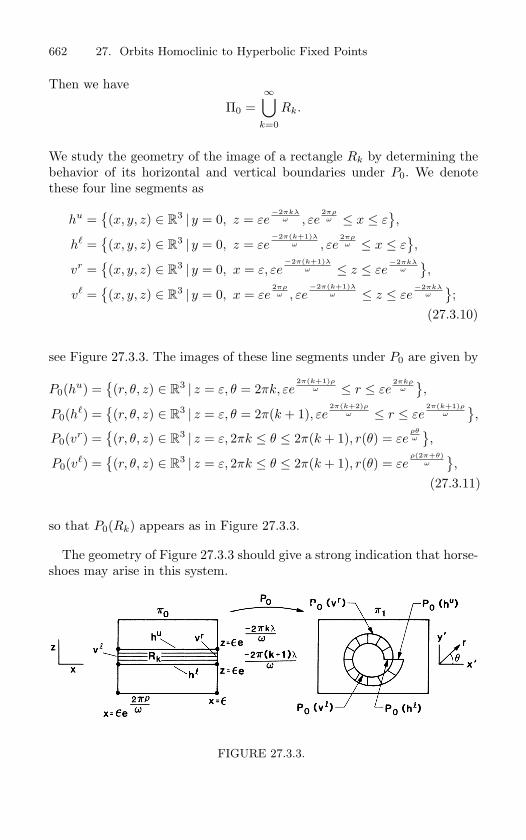
662 27. Orbits Homoclinic to Hyperbolic Fixed Points
Then we have
Π0 =∞⋃
k=0
Rk.
We study the geometry of the image of a rectangle Rk by determining thebehavior of its horizontal and vertical boundaries under P0. We denotethese four line segments as
hu =(x, y, z) ∈ R
3 | y = 0, z = εe−2πkλ
ω , εe2πρ
ω ≤ x ≤ ε,
h =(x, y, z) ∈ R
3 | y = 0, z = εe−2π(k+1)λ
ω , εe2πρ
ω ≤ x ≤ ε,
vr =(x, y, z) ∈ R
3 | y = 0, x = ε, εe−2π(k+1)λ
ω ≤ z ≤ εe−2πkλ
ω
,
v =(x, y, z) ∈ R
3 | y = 0, x = εe2πρ
ω , εe−2π(k+1)λ
ω ≤ z ≤ εe−2πkλ
ω
;
(27.3.10)
see Figure 27.3.3. The images of these line segments under P0 are given by
P0(hu) =(r, θ, z) ∈ R
3 | z = ε, θ = 2πk, εe2π(k+1)ρ
ω ≤ r ≤ εe2πkρ
ω
,
P0(h) =(r, θ, z) ∈ R
3 | z = ε, θ = 2π(k + 1), εe2π(k+2)ρ
ω ≤ r ≤ εe2π(k+1)ρ
ω
,
P0(vr) =(r, θ, z) ∈ R
3 | z = ε, 2πk ≤ θ ≤ 2π(k + 1), r(θ) = εeρθω
,
P0(v) =(r, θ, z) ∈ R
3 | z = ε, 2πk ≤ θ ≤ 2π(k + 1), r(θ) = εeρ(2π+θ)
ω
,
(27.3.11)
so that P0(Rk) appears as in Figure 27.3.3.
The geometry of Figure 27.3.3 should give a strong indication that horse-shoes may arise in this system.
FIGURE 27.3.3.
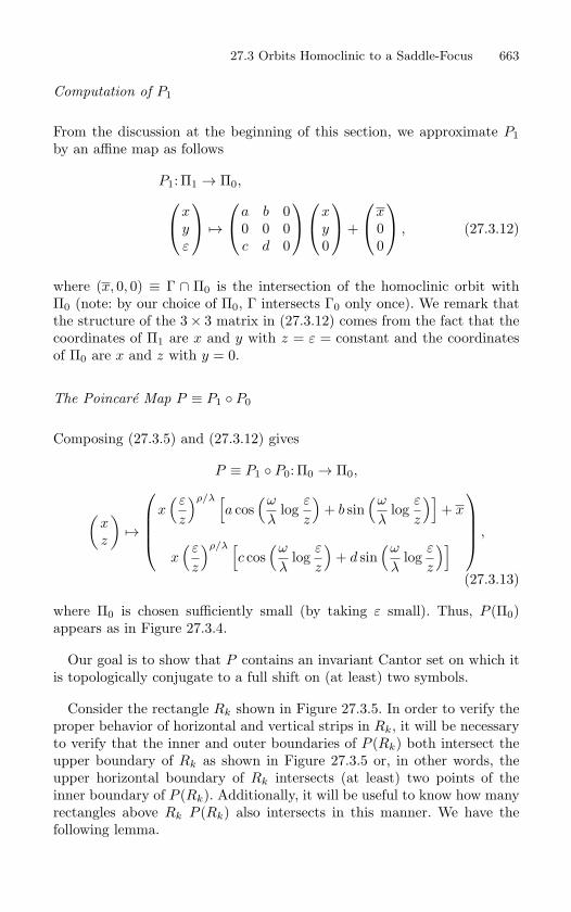
27.3 Orbits Homoclinic to a Saddle-Focus 663
Computation of P1
From the discussion at the beginning of this section, we approximate P1by an affine map as follows
P1: Π1 → Π0,x
yε
→
a b 0
0 0 0c d 0
x
y0
+
x
00
, (27.3.12)
where (x, 0, 0) ≡ Γ ∩ Π0 is the intersection of the homoclinic orbit withΠ0 (note: by our choice of Π0, Γ intersects Γ0 only once). We remark thatthe structure of the 3× 3 matrix in (27.3.12) comes from the fact that thecoordinates of Π1 are x and y with z = ε = constant and the coordinatesof Π0 are x and z with y = 0.
The Poincare Map P ≡ P1 P0
Composing (27.3.5) and (27.3.12) gives
P ≡ P1 P0: Π0 → Π0,
(xz
)→
x( ε
z
)ρ/λ [a cos
(ω
λlog
ε
z
)+ b sin
(ω
λlog
ε
z
)]+ x
x( ε
z
)ρ/λ [c cos
(ω
λlog
ε
z
)+ d sin
(ω
λlog
ε
z
)] ,
(27.3.13)
where Π0 is chosen sufficiently small (by taking ε small). Thus, P (Π0)appears as in Figure 27.3.4.
Our goal is to show that P contains an invariant Cantor set on which itis topologically conjugate to a full shift on (at least) two symbols.
Consider the rectangle Rk shown in Figure 27.3.5. In order to verify theproper behavior of horizontal and vertical strips in Rk, it will be necessaryto verify that the inner and outer boundaries of P (Rk) both intersect theupper boundary of Rk as shown in Figure 27.3.5 or, in other words, theupper horizontal boundary of Rk intersects (at least) two points of theinner boundary of P (Rk). Additionally, it will be useful to know how manyrectangles above Rk P (Rk) also intersects in this manner. We have thefollowing lemma.
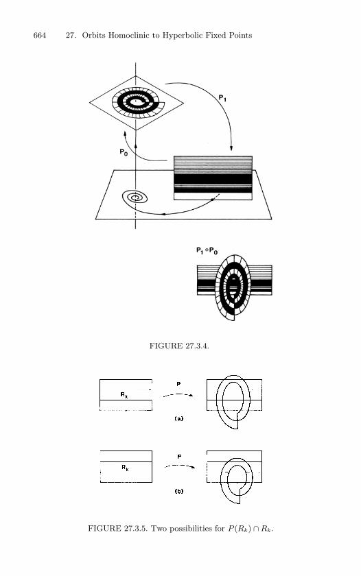
664 27. Orbits Homoclinic to Hyperbolic Fixed Points
FIGURE 27.3.4.
FIGURE 27.3.5. Two possibilities for P (Rk) ∩ Rk.
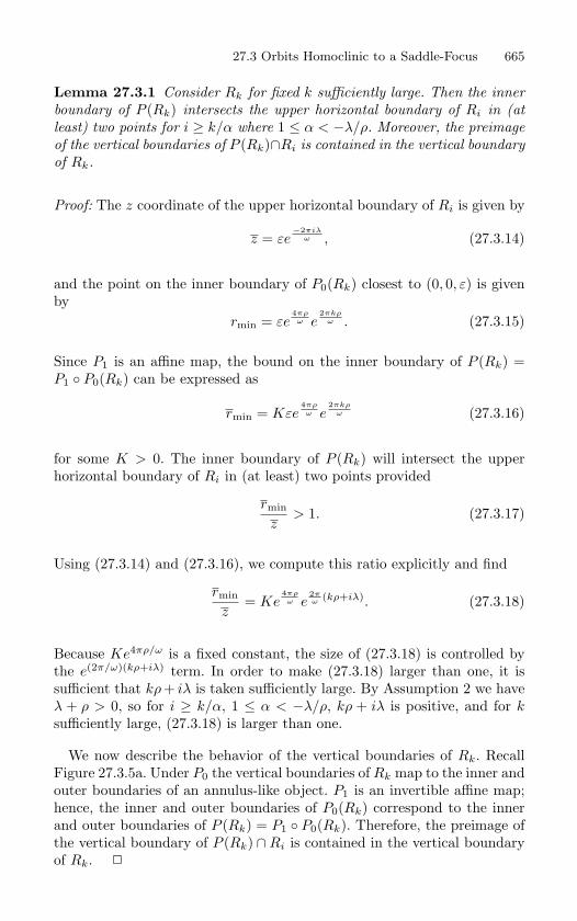
27.3 Orbits Homoclinic to a Saddle-Focus 665
Lemma 27.3.1 Consider Rk for fixed k sufficiently large. Then the inner
boundary of P (Rk) intersects the upper horizontal boundary of Ri in (at
least) two points for i ≥ k/α where 1 ≤ α < −λ/ρ. Moreover, the preimage
of the vertical boundaries of P (Rk)∩Ri is contained in the vertical boundary
of Rk.
Proof: The z coordinate of the upper horizontal boundary of Ri is given by
z = εe−2πiλ
ω , (27.3.14)
and the point on the inner boundary of P0(Rk) closest to (0, 0, ε) is givenby
rmin = εe4πρ
ω e2πkρ
ω . (27.3.15)
Since P1 is an affine map, the bound on the inner boundary of P (Rk) =P1 P0(Rk) can be expressed as
rmin = Kεe4πρ
ω e2πkρ
ω (27.3.16)
for some K > 0. The inner boundary of P (Rk) will intersect the upperhorizontal boundary of Ri in (at least) two points provided
rmin
z> 1. (27.3.17)
Using (27.3.14) and (27.3.16), we compute this ratio explicitly and find
rmin
z= Ke
4πρω e
2πω (kρ+iλ). (27.3.18)
Because Ke4πρ/ω is a fixed constant, the size of (27.3.18) is controlled bythe e(2π/ω)(kρ+iλ) term. In order to make (27.3.18) larger than one, it issufficient that kρ + iλ is taken sufficiently large. By Assumption 2 we haveλ + ρ > 0, so for i ≥ k/α, 1 ≤ α < −λ/ρ, kρ + iλ is positive, and for ksufficiently large, (27.3.18) is larger than one.
We now describe the behavior of the vertical boundaries of Rk. RecallFigure 27.3.5a. Under P0 the vertical boundaries of Rk map to the inner andouter boundaries of an annulus-like object. P1 is an invertible affine map;hence, the inner and outer boundaries of P0(Rk) correspond to the innerand outer boundaries of P (Rk) = P1 P0(Rk). Therefore, the preimage ofthe vertical boundary of P (Rk) ∩Ri is contained in the vertical boundaryof Rk.
666 27. Orbits Homoclinic to Hyperbolic Fixed Points
Lemma 27.3.1 points out the necessity of Assumption 2, since, if we hadinstead −ρ > λ > 0, then the image of Rk would fall below Rk for ksufficiently large, as shown in Figure 27.3.5b.
We now can state our main theorem.
Theorem 27.3.2 For k sufficiently large, Rk contains an invariant Can-
tor set, Λk, on which the Poincare map P is topologically conjugate to a
full shift on two symbols.
Proof: The proof is very similar to the proof of both Moser’s theorem(see Section 26) and Theorem 27.2.2. In Rk we must find two disjointµh-horizontal strips that are mapped over themselves in µv-vertical stripson which Assumptions 1 and 3 of Section 25 hold.
The fact that such µh-horizontal strips can be found on which Assump-tion 1 holds follows from Lemma 27.3.1. The fact that Assumption 3 holdsfollows from a calculation similar to that given in Moser’s theorem andTheorem 27.2.2. In the exercises we outline how one fills in the details ofthis proof.
We make several remarks.
Remark 1. The dynamics of P are often described by the phrase “P has acountable infinity of horseshoes.”
Remark 2. Note from Lemma 27.3.1 that the horseshoes in the different Rk
can interact. This would lead to different ways of setting up the symbolicdynamics. We will deal with this issue in the exercises.
Remark 3. If one were to break the homoclinic orbit with a perturbation,then only a finite number of the Λk would survive. We deal with this issuein the exercises.
27.3a The Bifurcation Analysis of Glendinningand Sparrow
Now that we have seen how complicated the orbit structure is in the neigh-borhood of an orbit homoclinic to a fixed point of saddle-focus type, wewant to get an understanding of how this situation occurs as the homo-clinic orbit is created. In this regard, the analysis given by Glendinningand Sparrow [1984] is insightful.
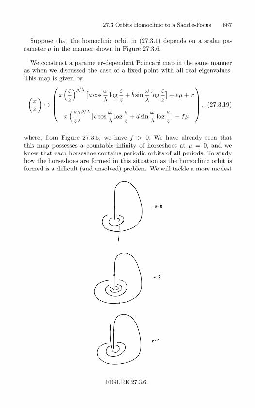
27.3 Orbits Homoclinic to a Saddle-Focus 667
Suppose that the homoclinic orbit in (27.3.1) depends on a scalar pa-rameter µ in the manner shown in Figure 27.3.6.
We construct a parameter-dependent Poincare map in the same manneras when we discussed the case of a fixed point with all real eigenvalues.This map is given by
(xz
)→
x( ε
z
)ρ/λ [a cos
ω
λlog
ε
z+ b sin
ω
λlog
ε
z
]+ eµ + x
x( ε
z
)ρ/λ [c cos
ω
λlog
ε
z+ d sin
ω
λlog
ε
z
]+ fµ
, (27.3.19)
where, from Figure 27.3.6, we have f > 0. We have already seen thatthis map possesses a countable infinity of horseshoes at µ = 0, and weknow that each horseshoe contains periodic orbits of all periods. To studyhow the horseshoes are formed in this situation as the homoclinic orbit isformed is a difficult (and unsolved) problem. We will tackle a more modest
FIGURE 27.3.6.
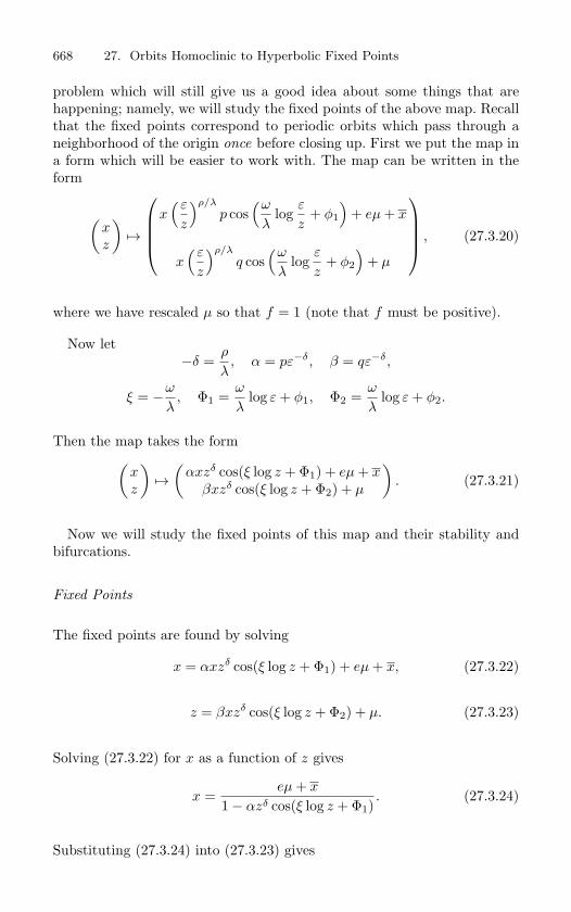
668 27. Orbits Homoclinic to Hyperbolic Fixed Points
problem which will still give us a good idea about some things that arehappening; namely, we will study the fixed points of the above map. Recallthat the fixed points correspond to periodic orbits which pass through aneighborhood of the origin once before closing up. First we put the map ina form which will be easier to work with. The map can be written in theform
(xz
)→
x( ε
z
)ρ/λ
p cos(ω
λlog
ε
z+ φ1
)+ eµ + x
x( ε
z
)ρ/λ
q cos(ω
λlog
ε
z+ φ2
)+ µ
, (27.3.20)
where we have rescaled µ so that f = 1 (note that f must be positive).
Now let−δ =
ρ
λ, α = pε−δ, β = qε−δ,
ξ = −ω
λ, Φ1 =
ω
λlog ε + φ1, Φ2 =
ω
λlog ε + φ2.
Then the map takes the form(xz
)→
(αxzδ cos(ξ log z + Φ1) + eµ + x
βxzδ cos(ξ log z + Φ2) + µ
). (27.3.21)
Now we will study the fixed points of this map and their stability andbifurcations.
Fixed Points
The fixed points are found by solving
x = αxzδ cos(ξ log z + Φ1) + eµ + x, (27.3.22)
z = βxzδ cos(ξ log z + Φ2) + µ. (27.3.23)
Solving (27.3.22) for x as a function of z gives
x =eµ + x
1− αzδ cos(ξ log z + Φ1). (27.3.24)
Substituting (27.3.24) into (27.3.23) gives
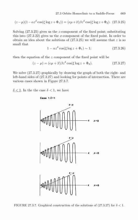
27.3 Orbits Homoclinic to a Saddle-Focus 669
(z−µ)(1−αzδ cos(ξ log z+Φ1)) = (eµ+x)βzδ cos(ξ log z+Φ2). (27.3.25)
Solving (27.3.25) gives us the z-component of the fixed point; substitutingthis into (27.3.22) gives us the x-component of the fixed point. In order toobtain an idea about the solutions of (27.3.25) we will assume that z is sosmall that
1− αzδ cos(ξ log z + Φ1) ∼ 1; (27.3.26)
then the equation of the z component of the fixed point will be
(z − µ) = (eµ + x)βzδ cos(ξ log z + Φ2). (27.3.27)
We solve (27.3.27) graphically by drawing the graph of both the right- andleft-hand sides of (27.3.27) and looking for points of intersection. There arevarious cases shown in Figure 27.3.7.
δ < 1. In the the case δ < 1, we have
FIGURE 27.3.7. Graphical construction of the solutions of (27.3.27) for δ < 1.
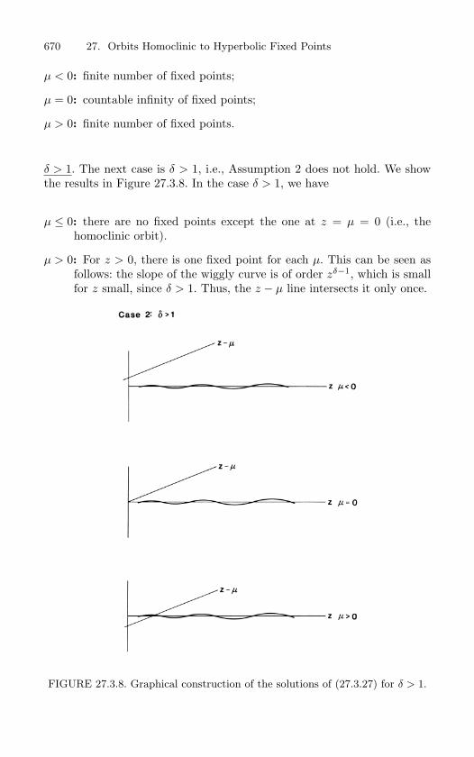
670 27. Orbits Homoclinic to Hyperbolic Fixed Points
µ < 0: finite number of fixed points;
µ = 0: countable infinity of fixed points;
µ > 0: finite number of fixed points.
δ > 1. The next case is δ > 1, i.e., Assumption 2 does not hold. We showthe results in Figure 27.3.8. In the case δ > 1, we have
µ ≤ 0: there are no fixed points except the one at z = µ = 0 (i.e., thehomoclinic orbit).
µ > 0: For z > 0, there is one fixed point for each µ. This can be seen asfollows: the slope of the wiggly curve is of order zδ−1, which is smallfor z small, since δ > 1. Thus, the z − µ line intersects it only once.
FIGURE 27.3.8. Graphical construction of the solutions of (27.3.27) for δ > 1.
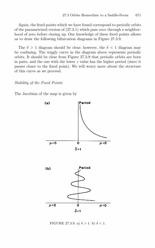
27.3 Orbits Homoclinic to a Saddle-Focus 671
Again, the fixed points which we have found correspond to periodic orbitsof the parametrized version of (27.3.1) which pass once through a neighbor-hood of zero before closing up. Our knowledge of these fixed points allowsus to draw the following bifurcation diagrams in Figure 27.3.9.
The δ > 1 diagram should be clear; however, the δ < 1 diagram maybe confusing. The wiggly curve in the diagram above represents periodicorbits. It should be clear from Figure 27.3.9 that periodic orbits are bornin pairs, and the one with the lower z value has the higher period (since itpasses closer to the fixed point). We will worry more about the structureof this curve as we proceed.
Stability of the Fixed Points
The Jacobian of the map is given by
FIGURE 27.3.9. a) δ > 1. b) δ < 1.
672 27. Orbits Homoclinic to Hyperbolic Fixed Points(A CD B
),
where
A = αzδ cos(ξ log z + Φ1),B = βxzδ−1[δ cos(ξ log z + Φ2)− ξ sin(ξ log z + Φ2)],C = αxzδ−1[δ cos(ξ log z + Φ1)− ξ sin(ξ log z + Φ1)],D = βzδ cos(ξ log z + Φ2).
(27.3.28)
The eigenvalues of the matrix are given by
λ1,2 =12
(A + B)±
√(A + B)2 − 4(AB − CD)
. (27.3.29)
δ > 1. For δ > 1, it should be clear that the eigenvalues will be small if z issmall (since both zδ and zδ−1 are small). Hence, for δ > 1, the one periodicorbit existing for µ > 0 is stable for µ small, and the homoclinic orbit atµ = 0 is an attractor.
The case δ < 1 is more complicated.
δ < 1. First notice that the determinant of the matrix given by AB − CDonly contains terms of order z2δ−1, so the map will be
area-contracting 12 < δ < 1,
area-expanding 0 < δ < 12 ,
for z sufficiently small.
We would thus expect different results in these two different δ ranges.
Now recall that the wiggly curve whose intersection with z − µ gave thefixed points was given by
(eµ + x)βzδ cos(ξ log z + Φ2).
Thus, from (27.3.28), a fixed point corresponding to a maximum of thiscurve corresponds to B = 0, and a fixed point corresponding to a zerocrossing of this curve corresponds to D = 0. We now want to look at thestability of fixed points satisfying these conditions.
D = 0. In this case λ1 = A, λ2 = B. Thus, for z small, λ1 is small and λ2is always large; hence, the fixed point is a saddle. Note in particular that,
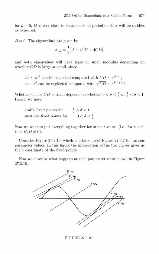
27.3 Orbits Homoclinic to a Saddle-Focus 673
for µ = 0, D is very close to zero; hence all periodic orbits will be saddlesas expected.
B = 0. The eigenvalues are given by
λ1,2 =12[A±
√A2 + 4CD
],
and both eigenvalues will have large or small modulus depending onwhether CD is large or small, since
A2 ∼ z2δ can be neglected compared with CD ∼ z2δ−1,A ∼ zδ can be neglected compared with
√CD ∼ zδ−(1/2).
Whether or not CD is small depends on whether 0 < δ < 12 or 1
2 < δ < 1.Hence, we have
stable fixed points for 12 < δ < 1.
unstable fixed points for 0 < δ < 12 .
Now we want to put everything together for other z values (i.e., for z suchthat B, D = 0).
Consider Figure 27.3.10, which is a blow-up of Figure 27.3.7 for variousparameter values. In this figure the intersection of the two curves gives usthe z coordinate of the fixed points.
Now we describe what happens at each parameter value shown in Figure27.3.10.
FIGURE 27.3.10.
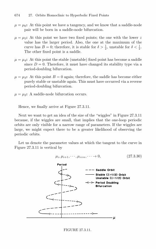
674 27. Orbits Homoclinic to Hyperbolic Fixed Points
µ = µ6: At this point we have a tangency, and we know that a saddle-nodepair will be born in a saddle-node bifurcation.
µ = µ5: At this point we have two fixed points; the one with the lower zvalue has the larger period. Also, the one at the maximum of thecurve has B = 0; therefore, it is stable for δ > 1
2 , unstable for δ < 12 .
The other fixed point is a saddle.
µ = µ4: At this point the stable (unstable) fixed point has become a saddlesince D = 0. Therefore, it must have changed its stability type via aperiod-doubling bifurcation.
µ = µ3: At this point B = 0 again; therefore, the saddle has become eitherpurely stable or unstable again. This must have occurred via a reverseperiod-doubling bifurcation.
µ = µ2: A saddle-node bifurcation occurs.
Hence, we finally arrive at Figure 27.3.11.
Next we want to get an idea of the size of the “wiggles” in Figure 27.3.11because, if the wiggles are small, that implies that the one-loop periodicorbits are only visible for a narrow range of parameters. If the wiggles arelarge, we might expect there to be a greater likelihood of observing theperiodic orbits.
Let us denote the parameter values at which the tangent to the curve inFigure 27.3.11 is vertical by
µi, µi+1, · · · , µi+n, · · · → 0, (27.3.30)
FIGURE 27.3.11.
27.3 Orbits Homoclinic to a Saddle-Focus 675
where the µi alternate in sign. Now recall that the z component of the fixedpoint was given by the solutions to the equations
z − µ = (eµ + x)βzδ cos(ξ log z + Φ2). (27.3.31)
Thus, we have
zi − µi = (eµi + x)βzδi cos(ξ log zi + Φ2), (27.3.32)
zi+1 − µi+1 = (eµi+1 + x)βzδi+1 cos(ξ log zi+1 + Φ2). (27.3.33)
From (27.3.32) and (27.3.33), we obtain
µi =zi − xβzδ
i cos(ξ log zi + Φ2)1 + eβzδ
i cos(ξ log zi + Φ2), (27.3.34)
µi+1 =zi+1 − xβzδ
i+1 cos(ξ log zi+1 + Φ2)1 + eβzδ
i+1 cos(ξ log zi+1 + Φ2). (27.3.35)
Now note that we have
ξ log zi+1 − ξ log zi ≈ π ⇒ zi+1
zi≈ exp
π
ξ, (27.3.36)
and we assume that z << 1 so that
1 + eβzδi(i+1) cos(ξ log zi(i+1) + Φ2) ∼ 1. (27.3.37)
Finally, we obtain
µi+1
µi=
zi+1 + [xβ cos(ξ log zi + Φ2)]zδi+1
zi − [xβ cos(ξ log zi + Φ2)]zδi
. (27.3.38)
Now, in the limit as z → 0, (27.3.38) becomes
µi+1
µi≈ −
(zi+1
zi
)δ
≈ − exp(
πδ
ξ
). (27.3.39)
Recall that δ = −ρ/λ, ξ = −ω/λ. We thus obtain
limi→∞
µi+1
µi= − exp
ρπ
ω. (27.3.40)
This quantity governs the size of the oscillations we see in Figure 27.3.11.
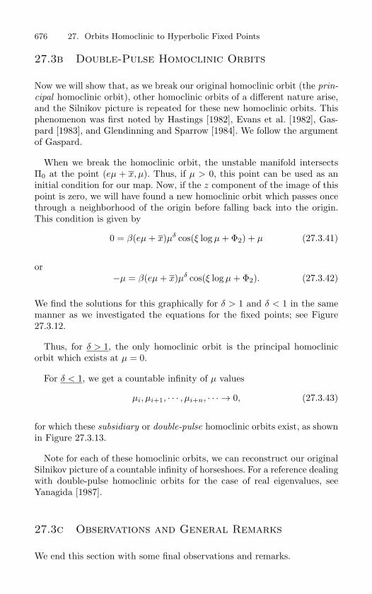
676 27. Orbits Homoclinic to Hyperbolic Fixed Points
27.3b Double-Pulse Homoclinic Orbits
Now we will show that, as we break our original homoclinic orbit (the prin-
cipal homoclinic orbit), other homoclinic orbits of a different nature arise,and the Silnikov picture is repeated for these new homoclinic orbits. Thisphenomenon was first noted by Hastings [1982], Evans et al. [1982], Gas-pard [1983], and Glendinning and Sparrow [1984]. We follow the argumentof Gaspard.
When we break the homoclinic orbit, the unstable manifold intersectsΠ0 at the point (eµ + x, µ). Thus, if µ > 0, this point can be used as aninitial condition for our map. Now, if the z component of the image of thispoint is zero, we will have found a new homoclinic orbit which passes oncethrough a neighborhood of the origin before falling back into the origin.This condition is given by
0 = β(eµ + x)µδ cos(ξ log µ + Φ2) + µ (27.3.41)
or−µ = β(eµ + x)µδ cos(ξ log µ + Φ2). (27.3.42)
We find the solutions for this graphically for δ > 1 and δ < 1 in the samemanner as we investigated the equations for the fixed points; see Figure27.3.12.
Thus, for δ > 1, the only homoclinic orbit is the principal homoclinicorbit which exists at µ = 0.
For δ < 1, we get a countable infinity of µ values
µi, µi+1, · · · , µi+n, · · · → 0, (27.3.43)
for which these subsidiary or double-pulse homoclinic orbits exist, as shownin Figure 27.3.13.
Note for each of these homoclinic orbits, we can reconstruct our originalSilnikov picture of a countable infinity of horseshoes. For a reference dealingwith double-pulse homoclinic orbits for the case of real eigenvalues, seeYanagida [1987].
27.3c Observations and General Remarks
We end this section with some final observations and remarks.
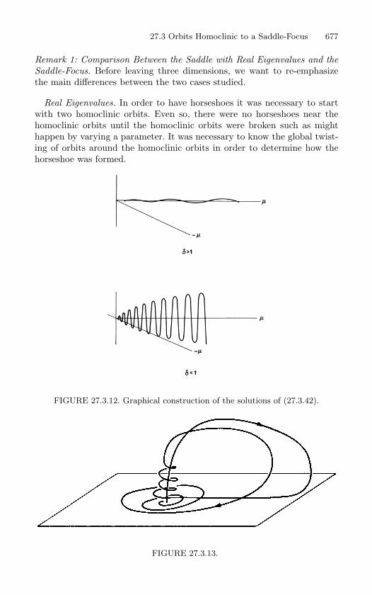
27.3 Orbits Homoclinic to a Saddle-Focus 677
Remark 1: Comparison Between the Saddle with Real Eigenvalues and the
Saddle-Focus. Before leaving three dimensions, we want to re-emphasizethe main differences between the two cases studied.
Real Eigenvalues. In order to have horseshoes it was necessary to startwith two homoclinic orbits. Even so, there were no horseshoes near thehomoclinic orbits until the homoclinic orbits were broken such as mighthappen by varying a parameter. It was necessary to know the global twist-ing of orbits around the homoclinic orbits in order to determine how thehorseshoe was formed.
FIGURE 27.3.12. Graphical construction of the solutions of (27.3.42).
FIGURE 27.3.13.
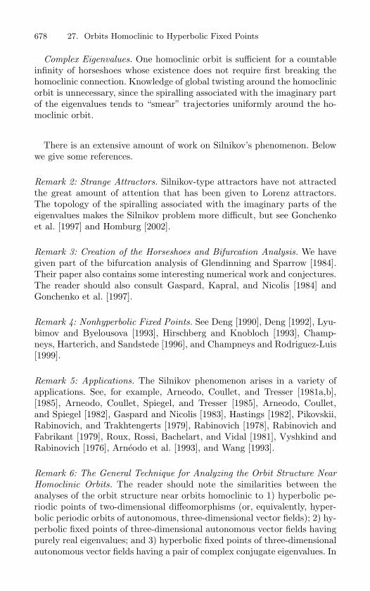
678 27. Orbits Homoclinic to Hyperbolic Fixed Points
Complex Eigenvalues. One homoclinic orbit is sufficient for a countableinfinity of horseshoes whose existence does not require first breaking thehomoclinic connection. Knowledge of global twisting around the homoclinicorbit is unnecessary, since the spiralling associated with the imaginary partof the eigenvalues tends to “smear” trajectories uniformly around the ho-moclinic orbit.
There is an extensive amount of work on Silnikov’s phenomenon. Belowwe give some references.
Remark 2: Strange Attractors. Silnikov-type attractors have not attractedthe great amount of attention that has been given to Lorenz attractors.The topology of the spiralling associated with the imaginary parts of theeigenvalues makes the Silnikov problem more difficult, but see Gonchenkoet al. [1997] and Homburg [2002].
Remark 3: Creation of the Horseshoes and Bifurcation Analysis. We havegiven part of the bifurcation analysis of Glendinning and Sparrow [1984].Their paper also contains some interesting numerical work and conjectures.The reader should also consult Gaspard, Kapral, and Nicolis [1984] andGonchenko et al. [1997].
Remark 4: Nonhyperbolic Fixed Points. See Deng [1990], Deng [1992], Lyu-bimov and Byelousova [1993], Hirschberg and Knobloch [1993], Champ-neys, Harterich, and Sandstede [1996], and Champneys and Rodriguez-Luis[1999].
Remark 5: Applications. The Silnikov phenomenon arises in a variety ofapplications. See, for example, Arneodo, Coullet, and Tresser [1981a,b],[1985], Arneodo, Coullet, Spiegel, and Tresser [1985], Arneodo, Coullet,and Spiegel [1982], Gaspard and Nicolis [1983], Hastings [1982], Pikovskii,Rabinovich, and Trakhtengerts [1979], Rabinovich [1978], Rabinovich andFabrikant [1979], Roux, Rossi, Bachelart, and Vidal [1981], Vyshkind andRabinovich [1976], Arneodo et al. [1993], and Wang [1993].
Remark 6: The General Technique for Analyzing the Orbit Structure Near
Homoclinic Orbits. The reader should note the similarities between theanalyses of the orbit structure near orbits homoclinic to 1) hyperbolic pe-riodic points of two-dimensional diffeomorphisms (or, equivalently, hyper-bolic periodic orbits of autonomous, three-dimensional vector fields); 2) hy-perbolic fixed points of three-dimensional autonomous vector fields havingpurely real eigenvalues; and 3) hyperbolic fixed points of three-dimensionalautonomous vector fields having a pair of complex conjugate eigenvalues. In
27.3 Orbits Homoclinic to a Saddle-Focus 679
all three cases a return map was constructed in a neighborhood of a pointalong the homoclinic orbit that consisted of the composition of two maps.One map described the dynamics near the hyperbolic invariant set (i.e., pe-riodic orbit or fixed point) and the other map described the dynamics nearthe homoclinic orbit outside of a neighborhood of the hyperbolic invariantset. Due to the fact that the fixed point is hyperbolic, the first map is wellapproximated from the linearization of the dynamical system (either mapor vector field) about the hyperbolic invariant set (either periodic orbitor fixed point). The second map, if we restrict ourselves to a sufficientlysmall neighborhood of the homoclinic orbit, is well approximated by anaffine map. In all cases, in order to show that chaotic invariant sets (moreprecisely, an invarant Cantor set on which the dynamics are topologicallyconjugate to a full shift on N symbols) are present near the homoclinicorbit, we find N µh-horizontal strips that are mapped over themselves inµv-vertical strips so that Assumptions 1 and 3 of Chapter 25 hold. Thenature of the map near the hyperbolic invariant set is responsible for theverification of Assumption 3 (i.e., expansion and contraction in the appro-priate directions). The nature of the map outside of the hyperbolic invariantset is responsible for the verification of Assumption 1. However, note thatin the case of transversal orbits homoclinic to hyperbolic periodic orbits ofn-dimensional diffeomorphisms, we did not need any special assumptionson the eigenvalues of the periodic orbit or the nature of the intersection ofthe stable and unstable manifolds (hyperbolicity and transversality weresufficient). This is very different from the situation of orbits homoclinic tohyperbolic fixed points of autonomous vector fields, where special assump-tions on the relative magnitudes of the eigenvalues at the fixed point andthe nature of the (nontransversal) homoclinic orbit(s) were necessary.
Remark 7: Higher Dimensional Results. For generalizations to orbits ho-moclinic to hyperbolic fixed points of n-dimensional (n ≥ 4) autonomousvector fields, the reader should consult Turaev and Silnikov [1987], Ovsyan-nikov and Silnikov [1987], Deng [1989a], [1989b], [1993], Chow, Deng, andFiedler [1990], Ovsyannikov and Silnikov [1992], Arnold et al. [1994],andHomburg [1996], Glendinning [1997], Ashwin [1997], Ragazzo [1997], Laingand Glendinning [1997], Fowler [1990], Chernyshev [1985], and Glendinningand Laing [1996].
Remark 8: Numerical Methods. See Champneys, Kuznetsov, and Sandst-ede [1996] for a review of numerical methods for computing homoclinicorbits. See also Beyn and Kleinkauf [1997], Liu et al. [1997], and Doedeland Friedman [1989].
Remark 9: N-Pulse Homoclinic Orbits. In recent years there has been agreat deal of work on N-pulse homoclinic orbits or “multi-bump” orbits. See
680 27. Orbits Homoclinic to Hyperbolic Fixed Points
Champneys [1994], Zelati and Nolasco [1999], Camassa et al. [1998], Bolotinand MacKay [1997], Rabinowitz [1997], Soto Trevino and Kaper [1996],Kaper and Kovacic [1996], Haller and Wiggins [1995], and Glendinning[1989].
Remark 10: Global Center Manifold Techniques. Recently generalizationsof the local center manifold techniques to a global setting valid in theneighborhood of a homoclinic orbit have been developed. See Sandstede[1993], Homburg [1996], Shaskov and Turaev [1999], and Chow et al. [2000].
Remark 10: Heteroclinic Cycles. See Wiggins [1988] and Tresser [1984] forsome general results in R
3. Devaney [1976] discusses some heteroclinic cy-cles in Hamiltonian systems. Heteroclinic cycles frequently arise in applica-tions. For example, they appear to be the mechanism giving rise to “burst-ing” in a model for the interaction of eddies in the boundary layer of fluidflow near a wall, see Aubry, Holmes, and Lumley [1988] and Guckenheimerand Holmes [1988]. See also Tian and Du [2000], Koon et al. [2000], Hom-burg [2000], Ashwin and Field [1999], Chossat et al. [1999], Woods andChampneys [1999], Chow et al [1999], Sun and Kooij [1998], Qi and Jing[1998], Han [1998], Ashwin and Chossat [1998], Belykh and Bykov [1998],Zimmermann and Natiello [1998], Chernyshev [1997], Krupa [1997], Houand Golubitsky [1997], Chossat et al. [1997], Maxwell [1997], Zhu [ 1996],Lauterbach et al. [1996], Worfolk [1996], Blazquez and Tuma [1996], Bat-teli [1994], Krupa and Melbourne [1995], Lauterbach and Roberts [1992],McCord and Mischaikow [1992], Field and Swift [1991], Feng [1991], Chos-sat and Armbruster [1991], Campbell and Holmes [1991], Armbruster andChossatt [ 1991], and Deng [1991].
Remark 11: Homoclinic Orbits in Hamiltonian and Reversible Systems.
Early work on homoclinic orbits in Hamiltonian systems can be found inDevaney [1976], [1978], Holmes [1980], and Wiggins [1988]. There has beena great deal of additional work in these areas over the past 10 years. SeeChampneys and Harterich [2000], Zhang [2000], Bolle and Buffoni [1999],Arioli and Szulkin [1999], Ding and Willem [1999], Ding and Girardi [1999],Koltsova and Lerman [1998], Ding [1998], Koltsova and Lerman [1996],Koltsova and Lerman [1995], Ragazzo [1997], Mielke et al. [1992], Lerman[1991], Buffoni [1993], Champneys and Toland [1993], Lerman [1989], andTuraev and Silnikov [1989] . For some results for reversible systems seeAfendikov and Mielke [1999], Iooss [1997], and Chirchill and Rod [1986].
27.4 Exercises 681
27.4 Exercises
1. Recall the discussion in Section 27.2 and specifically the vector field (27.2.1). Wouldthere be any qualitative changes in the results of these sections if the eigenvaluesdepended on the parameter µ? How would this situation best be handled?
2. Show that generically for λ2 > λ1, the homoclinic orbit in (27.2.1) for µ = 0 is tangentto the y axis in the x − y plane at the origin.
Construct a nongeneric example where this does not occur and explain why yourexample is not generic. (Hint: find an appropriate symmetry.)
3. In Equation (27.2.10) we took
11 − Az|λ1|/λ3
∼ 1 as z → 0.
Show that if instead we take
11 − Az|λ1|/λ3
= 1 + Az|λ1|/λ3 + · · ·
our results are not affected for z sufficiently small.
4. From Section 27.2, consider the case λ2 < λ1. Show that in this case the homoclinicorbit of (27.2.1) is tangent to the x-axis at the origin in the x − y plane. Construct aPoincare map near the homoclinic orbit following Section 27.2 and show that Theorem27.2.1 still holds. In describing the “half-bowtie” shape of P0(Π0) in Π1, compare itwith the case λ1 < λ2.
5. From Section 27.2, consider the case λ2 = λ1. Describe the geometry of the return ofthe homoclinic orbit to the origin. Construct a Poincare map following Section 27.2and show that Theorem 27.2.1 still holds. In describing the “half-bowtie” shape ofP0(Π0) in Π1, compare it with the cases λ1 > λ2 and λ2 < λ1.
6. Argue that if (27.2.1) possesses only one homoclinic orbit, then the Poincare mapdefined near the homoclinic orbit cannot possess an invariant Cantor set on which itis topologically conjugate to a full shift on N (N ≥ 2) symbols.
7. Recall the discussion in Section 27.2a. In Assumption 1′, discuss the necessity andgeometry behind the requirement d = 0.
8. Work out all of the details in the proof of Theorem 27.2.2. (Hint: mimic the proof ofMoser’s theorem in Section 26.)
9. Recall the discussion in Section 27.2a. Suppose we instead chose configuration b) inFigure 27.2.9 with Assumption 1′ and Assumption 2′ still holding. Is Theorem 27.2.2still valid in this case? If so, what modifications must be made in order to carry outthe proof?
10. Work out all of the details in the proof of Theorem 27.3.2. (Hint: mimic the proof ofMoser’s theorem in Section 26.)
11. In Theorem 27.3.2 we proved the existence of an invariant Cantor set Λk ⊂ Rk suchthat the Poincare map restricted to Λk was topologically conjugate to a full shift ontwo symbols. This was true for all k sufficiently large. Show that Theorem 27.3.2 can bemodified (in particular, the choice of µh-horizontal and µv-vertical strips) so that Π0contains an invariant Cantor set on which the Poincare map is topologically conjugateto a full shift on N symbols with N arbitrarily large. (Hint: use Lemma 27.3.1 and seeWiggins [1988] if you need help.)
Is there a difference in the dynamics of this invariant set and the dynamics in⋃
k≥k0Λk
constructed in Theorem 27.3.2?
682 27. Orbits Homoclinic to Hyperbolic Fixed Points
12. Recall the construction in Theorem 27.3.2. Suppose the Poincare map P is perturbed(as might occur in a one-parameter family). Show that, for sufficiently small pertur-bations, an infinite number of the Λk are destroyed yet a finite number survive. Doesthis contradict the fact that horseshoes are structurally stable?
13. Recall the discussion in Section 27.3. Suppose (27.3.1) is invariant under the coordinatetransformation
(x, y, z) → (−x, −y, −z)
with Assumptions 1 and 3 still holding.
a) Show that (27.3.1) must possess two orbits homoclinic to the origin. Draw thetwo homoclinic orbits in the phase space. Denote the homoclinic orbits by Γ0and Γ1.
b) Construct a Poincare map in a neighborhood of Γ0∪Γ1∪(0, 0, 0) and show thatthe map has an invariant Cantor set on which the dynamics are topologicallyconjugate to a full shift on two symbols.
c) If we denote the two symbols by 0 and 1, show that the motion in phase spaceis such that a ‘0’ corresponds to a trajectory following close to Γ0 and a ‘1’corresponds to a trajectory following close to Γ1. Hence, give a geometricaldescription of the manifestation of chaos in phase space. (See Wiggins [1988] ifyou need help.)
14. Consider our description of the bifurcation analysis of Glendinning and Sparrow. Jus-tify the curves shown in Figure 27.3.9.
15. Consider the sequence of bifurcations discussed in Figure 27.3.10. Explain why aperiod-doubling bifurcation occurs after µ5 and a reverse period-doubling bifurcationoccurs before µ3.
16. Suppose we reverse the direction of time in (27.3.1), i.e., we let
t → −t,
with Assumptions 1 and 2 still holding. Describe the dynamics near the homoclinicorbit.
17. Consider the vector field (27.3.1). Suppose that Assumption 1 holds but Assumption2 is replaced by the following.
Assumption 2 ′. −ρ > λ > 0.
Describe the dynamics near the homoclinic orbit. (See Holmes [1980] for help.)
18. Consider a Cr (r as large as necessary) autonomous vector field in R3. We denote
coordinates in R3 by x − y − z. Suppose the vector field has two hyperbolic fixed
points, p1 and p2, respectively, in the x − y plane.
Local Assumption: The vector field linearized at p1 has the form
x = λ1x,y = λ2y,z = λ3z,
with λ1 > 0, λ3 < λ2 < 0.
The vector field linearized at p2 has the form
x = ρx − ωy,y = ωx + ρy,z = λz,
with ρ < 0, λ > 0, ω = 0.
Global Assumption: p1 and p2 are connected by a heteroclinic orbit, denoted Γ12 thatlies in the x − y plane.
p2 and p1 are connected by a heteroclinic orbit, Γ21, that lies outside the plane; seeFigure 27.4.1.
Thus, Γ12 ∪ Γ21 ∪ p1 ∪ p2 form a heteroclinic cycle. The goal is to construct aPoincare map, P , in a neighborhood of the heteroclinic cycle and prove the followingtheorem.
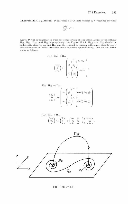
27.4 Exercises 683
Theorem 27.4.1 (Tresser) P possesses a countable number of horseshoes provided
ρλ2
λλ1< 1.
(Hint: P will be constructed from the composition of four maps. Define cross sectionsΠ01, Π11, Π12, and Π02 appropriately; see Figure 27.4.1. Π0,1 and Π11 should besufficiently close to p1, and Π12 and Π02 should be chosen sufficiently close to p2. Ifthe coordinates on these cross-sections are chosen appropriately, then we can derivemaps as follows
P01: Π01 → Π1,
(x1εz1
)→
ε
ε
ε
x1
λ2/λ1
z1
ε
x1
λ3/λ1
,
P02: Π02 → Π12,
(x20z2
)→
x2
ε
z2
ρ/λ
cos ωλ log ε
z2
x2
ε
z2
ρ/λ
sin ωλ log ε
z2
ε
,
P12: Π12 → Π01,(x2y2ε
)→
( 00ε
)+
(a2 b2 0c2 d2 00 0 0
)(x2y20
),
FIGURE 27.4.1.
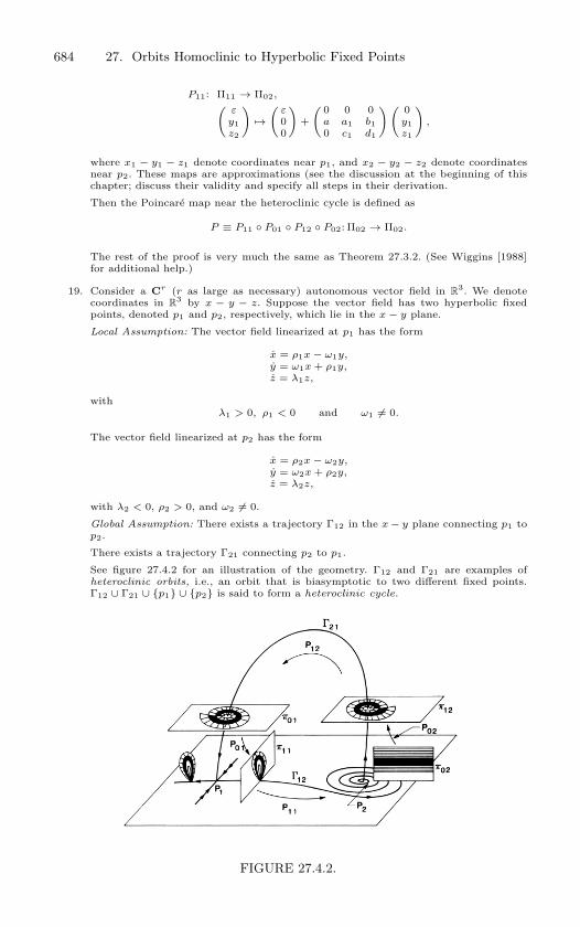
684 27. Orbits Homoclinic to Hyperbolic Fixed Points
P11: Π11 → Π02,(εy1z2
)→
(ε00
)+
( 0 0 0a a1 b10 c1 d1
)( 0y1z1
),
where x1 − y1 − z1 denote coordinates near p1, and x2 − y2 − z2 denote coordinatesnear p2. These maps are approximations (see the discussion at the beginning of thischapter; discuss their validity and specify all steps in their derivation.
Then the Poincare map near the heteroclinic cycle is defined as
P ≡ P11 P01 P12 P02: Π02 → Π02.
The rest of the proof is very much the same as Theorem 27.3.2. (See Wiggins [1988]for additional help.)
19. Consider a Cr (r as large as necessary) autonomous vector field in R3. We denote
coordinates in R3 by x − y − z. Suppose the vector field has two hyperbolic fixed
points, denoted p1 and p2, respectively, which lie in the x − y plane.
Local Assumption: The vector field linearized at p1 has the form
x = ρ1x − ω1y,y = ω1x + ρ1y,z = λ1z,
withλ1 > 0, ρ1 < 0 and ω1 = 0.
The vector field linearized at p2 has the form
x = ρ2x − ω2y,y = ω2x + ρ2y,z = λ2z,
with λ2 < 0, ρ2 > 0, and ω2 = 0.
Global Assumption: There exists a trajectory Γ12 in the x − y plane connecting p1 top2.
There exists a trajectory Γ21 connecting p2 to p1.
See figure 27.4.2 for an illustration of the geometry. Γ12 and Γ21 are examples ofheteroclinic orbits, i.e., an orbit that is biasymptotic to two different fixed points.Γ12 ∪ Γ21 ∪ p1 ∪ p2 is said to form a heteroclinic cycle.
FIGURE 27.4.2.
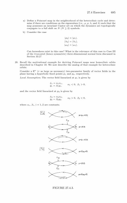
27.4 Exercises 685
a) Define a Poincare map in the neighborhood of the heteroclinic cycle and deter-mine if there are conditions on the eigenvalues (i.e., ρ, ρ, λ, and λ) such that themap possesses an invariant Cantor set on which the dynamics are topologicallyconjugate to a full shift on N (N ≥ 2) symbols.
b) Consider the case
|ρ2| = |ρ1|,|λ2| = |λ1|,|ω2| = |ω1|.
Can horseshoes exist in this case? What is the relevance of this case to Case IIIof the truncated (hence symmetric) three-dimensional normal form discussed inSection 33.2?
20. Recall the motivational example for deriving Poincare maps near homoclinic orbitsdescribed in Chapter 10. We now describe the analog of that example for heteroclinicorbits.
Consider a Cr (r as large as necessary) two-parameter family of vector fields in theplane having a hyperbolic fixed points p1 and p2, respectively.
Local Assumption: The vector field linearized at p1 is given by
x1 = α1x1,y1 = β1y1,
α1 < 0, β1 > 0,
and the vector field linearized at p2 is given by
x2 = α2x2,y2 = β2y2,
α2 > 0, β2 < 0,
where αi, βi, i = 1, 2 are constants.
FIGURE 27.4.3.
686 27. Orbits Homoclinic to Hyperbolic Fixed Points
Global Assumption. p1 and p2 are connected by a heteroclinic cycle. We denote theheteroclinic orbit going from p1 to p2 in positive time by Γ12 and the heteroclinic orbitgoing from p2 to p1 in positive time by Γ21.
The heteroclinic cycle depends on the parameters as follows. For µ ≡ (µ1, µ2), let Nbe a neighborhood of zero in the µ1, µ2 plane; then we assume the following.
1) Γ12 exists for all µ ∈ (µ1, µ2) | µ1 = 0 ∩ N ≡ N1.
2) Γ21 exists for all µ ∈ (µ1, µ2) | µ2 = 0 ∩ N ≡ N2.
Furthermore, we assume that Γ12 and Γ21 break “transversely” as shown in Figure27.4.3.
Construct a two-parameter family of Poincare maps near the heteroclinic cycle andstudy the bifurcation and stability of periodic orbits.
28
Melnikov’s Method forHomoclinic Orbits inTwo-Dimensional,Time-Periodic Vector Fields
We have seen that transverse homoclinic orbits to hyperbolic periodicpoints of two-dimensional maps gives rise to chaotic dynamics in the senseof Theorems 26.0.5 and 26.0.6. We will now develop a perturbation methodoriginally due to Melnikov [1963] for proving the existence of transverse ho-moclinic orbits to hyperbolic periodic orbits in a class of two-dimensional,time-periodic vector fields; then by considering a Poincare map, Theorems26.0.5 and 26.0.6 can be applied to conclude that the system possesseschaotic dynamics.
28.1 The General Theory
We consider the following class of systems:
x =∂H
∂y(x, y) + εg1(x, y, t, ε),
y = −∂H
∂x(x, y) + εg2(x, y, t, ε), (x, y) ∈ R
2; (28.1.1)
or, in vector form,q = JDH(q) + εg(q, t, ε), (28.1.2)
where q = (x, y), DH = (∂H∂x , ∂H
∂y ), g = (g1, g2), and
J =(
0 1−1 0
).
We assume that (28.1.1) is sufficiently differentiable (Cr, r ≥ 2 will do) on
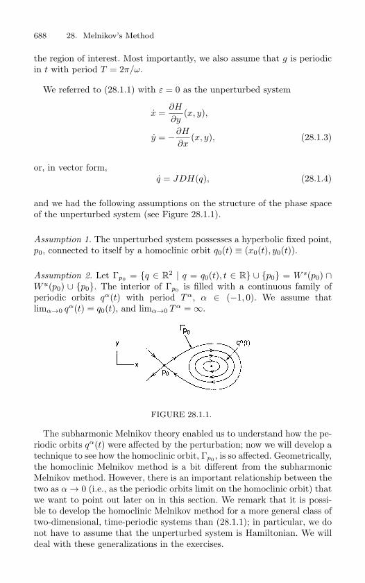
688 28. Melnikov’s Method
the region of interest. Most importantly, we also assume that g is periodicin t with period T = 2π/ω.
We referred to (28.1.1) with ε = 0 as the unperturbed system
x =∂H
∂y(x, y),
y = −∂H
∂x(x, y), (28.1.3)
or, in vector form,q = JDH(q), (28.1.4)
and we had the following assumptions on the structure of the phase spaceof the unperturbed system (see Figure 28.1.1).
Assumption 1. The unperturbed system possesses a hyperbolic fixed point,p0, connected to itself by a homoclinic orbit q0(t) ≡ (x0(t), y0(t)).
Assumption 2. Let Γp0 = q ∈ R2 | q = q0(t), t ∈ R ∪ p0 = W s(p0) ∩
Wu(p0) ∪ p0. The interior of Γp0 is filled with a continuous family ofperiodic orbits qα(t) with period Tα, α ∈ (−1, 0). We assume thatlimα→0 qα(t) = q0(t), and limα→0 Tα = ∞.
FIGURE 28.1.1.
The subharmonic Melnikov theory enabled us to understand how the pe-riodic orbits qα(t) were affected by the perturbation; now we will develop atechnique to see how the homoclinic orbit, Γp0 , is so affected. Geometrically,the homoclinic Melnikov method is a bit different from the subharmonicMelnikov method. However, there is an important relationship between thetwo as α → 0 (i.e., as the periodic orbits limit on the homoclinic orbit) thatwe want to point out later on in this section. We remark that it is possi-ble to develop the homoclinic Melnikov method for a more general class oftwo-dimensional, time-periodic systems than (28.1.1); in particular, we donot have to assume that the unperturbed system is Hamiltonian. We willdeal with these generalizations in the exercises.
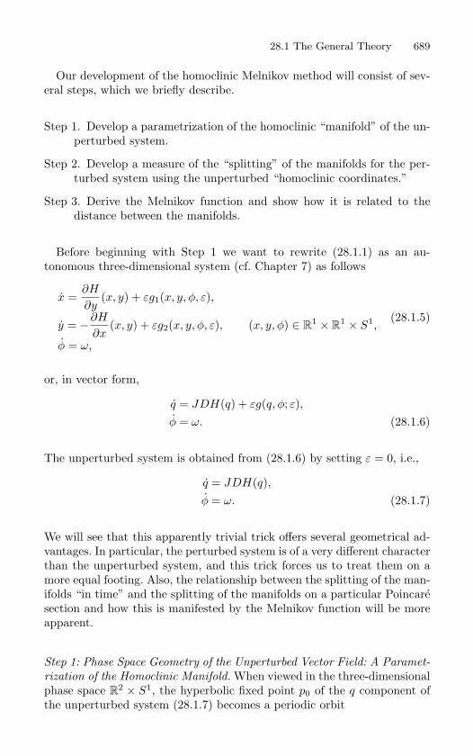
28.1 The General Theory 689
Our development of the homoclinic Melnikov method will consist of sev-eral steps, which we briefly describe.
Step 1. Develop a parametrization of the homoclinic “manifold” of the un-perturbed system.
Step 2. Develop a measure of the “splitting” of the manifolds for the per-turbed system using the unperturbed “homoclinic coordinates.”
Step 3. Derive the Melnikov function and show how it is related to thedistance between the manifolds.
Before beginning with Step 1 we want to rewrite (28.1.1) as an au-tonomous three-dimensional system (cf. Chapter 7) as follows
x =∂H
∂y(x, y) + εg1(x, y, φ, ε),
y = −∂H
∂x(x, y) + εg2(x, y, φ, ε), (x, y, φ) ∈ R
1 × R1 × S1,
φ = ω,
(28.1.5)
or, in vector form,
q = JDH(q) + εg(q, φ; ε),φ = ω. (28.1.6)
The unperturbed system is obtained from (28.1.6) by setting ε = 0, i.e.,
q = JDH(q),φ = ω. (28.1.7)
We will see that this apparently trivial trick offers several geometrical ad-vantages. In particular, the perturbed system is of a very different characterthan the unperturbed system, and this trick forces us to treat them on amore equal footing. Also, the relationship between the splitting of the man-ifolds “in time” and the splitting of the manifolds on a particular Poincaresection and how this is manifested by the Melnikov function will be moreapparent.
Step 1: Phase Space Geometry of the Unperturbed Vector Field: A Paramet-
rization of the Homoclinic Manifold. When viewed in the three-dimensionalphase space R
2 × S1, the hyperbolic fixed point p0 of the q component ofthe unperturbed system (28.1.7) becomes a periodic orbit
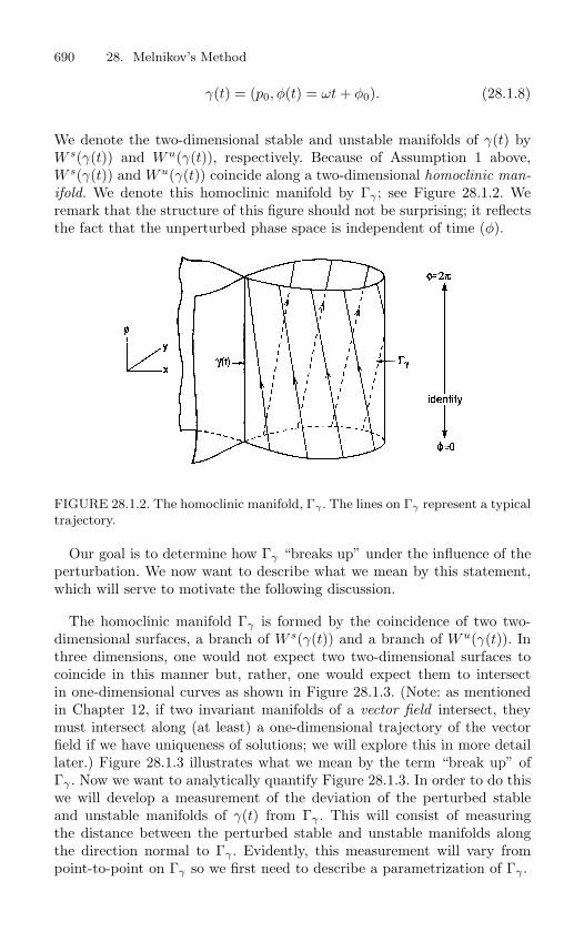
690 28. Melnikov’s Method
γ(t) = (p0, φ(t) = ωt + φ0). (28.1.8)
We denote the two-dimensional stable and unstable manifolds of γ(t) byW s(γ(t)) and Wu(γ(t)), respectively. Because of Assumption 1 above,W s(γ(t)) and Wu(γ(t)) coincide along a two-dimensional homoclinic man-
ifold. We denote this homoclinic manifold by Γγ ; see Figure 28.1.2. Weremark that the structure of this figure should not be surprising; it reflectsthe fact that the unperturbed phase space is independent of time (φ).
FIGURE 28.1.2. The homoclinic manifold, Γγ . The lines on Γγ represent a typical
trajectory.
Our goal is to determine how Γγ “breaks up” under the influence of theperturbation. We now want to describe what we mean by this statement,which will serve to motivate the following discussion.
The homoclinic manifold Γγ is formed by the coincidence of two two-dimensional surfaces, a branch of W s(γ(t)) and a branch of Wu(γ(t)). Inthree dimensions, one would not expect two two-dimensional surfaces tocoincide in this manner but, rather, one would expect them to intersectin one-dimensional curves as shown in Figure 28.1.3. (Note: as mentionedin Chapter 12, if two invariant manifolds of a vector field intersect, theymust intersect along (at least) a one-dimensional trajectory of the vectorfield if we have uniqueness of solutions; we will explore this in more detaillater.) Figure 28.1.3 illustrates what we mean by the term “break up” ofΓγ . Now we want to analytically quantify Figure 28.1.3. In order to do thiswe will develop a measurement of the deviation of the perturbed stableand unstable manifolds of γ(t) from Γγ . This will consist of measuringthe distance between the perturbed stable and unstable manifolds alongthe direction normal to Γγ . Evidently, this measurement will vary frompoint-to-point on Γγ so we first need to describe a parametrization of Γγ .
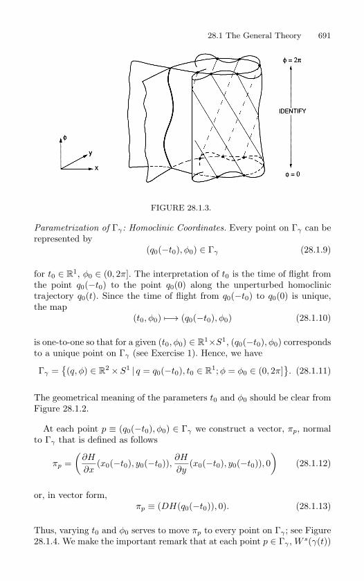
28.1 The General Theory 691
FIGURE 28.1.3.
Parametrization of Γγ : Homoclinic Coordinates. Every point on Γγ can berepresented by
(q0(−t0), φ0) ∈ Γγ (28.1.9)
for t0 ∈ R1, φ0 ∈ (0, 2π]. The interpretation of t0 is the time of flight from
the point q0(−t0) to the point q0(0) along the unperturbed homoclinictrajectory q0(t). Since the time of flight from q0(−t0) to q0(0) is unique,the map
(t0, φ0) −→ (q0(−t0), φ0) (28.1.10)
is one-to-one so that for a given (t0, φ0) ∈ R1×S1, (q0(−t0), φ0) corresponds
to a unique point on Γγ (see Exercise 1). Hence, we have
Γγ =(q, φ) ∈ R
2 × S1 | q = q0(−t0), t0 ∈ R1;φ = φ0 ∈ (0, 2π]
. (28.1.11)
The geometrical meaning of the parameters t0 and φ0 should be clear fromFigure 28.1.2.
At each point p ≡ (q0(−t0), φ0) ∈ Γγ we construct a vector, πp, normalto Γγ that is defined as follows
πp =(
∂H
∂x(x0(−t0), y0(−t0)),
∂H
∂y(x0(−t0), y0(−t0)), 0
)(28.1.12)
or, in vector form,πp ≡ (DH(q0(−t0)), 0). (28.1.13)
Thus, varying t0 and φ0 serves to move πp to every point on Γγ ; see Figure28.1.4. We make the important remark that at each point p ∈ Γγ , W s(γ(t))
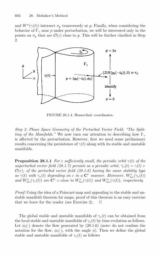
692 28. Melnikov’s Method
and Wu(γ(t)) intersect πp transversely at p. Finally, when considering thebehavior of Γγ near p under perturbation, we will be interested only in thepoints on πp that are O(ε) close to p. This will be further clarified in Step2.
FIGURE 28.1.4. Homoclinic coordinates.
Step 2: Phase Space Geometry of the Perturbed Vector Field: “The Split-
ting of the Manifolds.” We now turn our attention to describing how Γγ
is affected by the perturbation. However, first we need some preliminaryresults concerning the persistence of γ(t) along with its stable and unstablemanifolds.
Proposition 28.1.1 For ε sufficiently small, the periodic orbit γ(t) of the
unperturbed vector field (28.1.7) persists as a periodic orbit, γε(t) = γ(t) +O(ε), of the perturbed vector field (28.1.6) having the same stability type
as γ(t) with γε(t) depending on ε in a Cr manner. Moreover, W sloc(γε(t))
and Wuloc(γε(t)) are Cr ε-close to W s
loc(γ(t)) and Wuloc(γ(t)), respectively.
Proof: Using the idea of a Poincare map and appealing to the stable and un-stable manifold theorem for maps, proof of this theorem is an easy exercisethat we leave for the reader (see Exercise 2).
The global stable and unstable manifolds of γε(t) can be obtained fromthe local stable and unstable manifolds of γε(t) by time evolution as follows.Let φt(·) denote the flow generated by (28.1.6) (note: do not confuse thenotation for the flow, φt(·), with the angle φ). Then we define the globalstable and unstable manifolds of γε(t) as follows
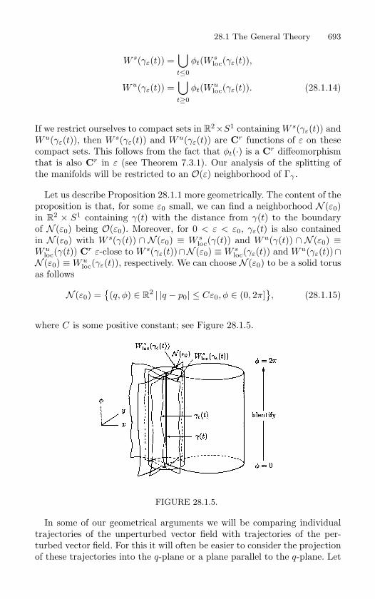
28.1 The General Theory 693
W s(γε(t)) =⋃t≤0
φt(W sloc(γε(t)),
Wu(γε(t)) =⋃t≥0
φt(Wuloc(γε(t)). (28.1.14)
If we restrict ourselves to compact sets in R2×S1 containing W s(γε(t)) and
Wu(γε(t)), then W s(γε(t)) and Wu(γε(t)) are Cr functions of ε on thesecompact sets. This follows from the fact that φt(·) is a Cr diffeomorphismthat is also Cr in ε (see Theorem 7.3.1). Our analysis of the splitting ofthe manifolds will be restricted to an O(ε) neighborhood of Γγ .
Let us describe Proposition 28.1.1 more geometrically. The content of theproposition is that, for some ε0 small, we can find a neighborhood N (ε0)in R
2 × S1 containing γ(t) with the distance from γ(t) to the boundaryof N (ε0) being O(ε0). Moreover, for 0 < ε < ε0, γε(t) is also containedin N (ε0) with W s(γ(t)) ∩ N (ε0) ≡ W s
loc(γ(t)) and Wu(γ(t)) ∩ N (ε0) ≡Wu
loc(γ(t)) Cr ε-close to W s(γε(t))∩N (ε0) ≡ W sloc(γε(t)) and Wu(γε(t))∩
N (ε0) ≡ Wuloc(γε(t)), respectively. We can choose N (ε0) to be a solid torus
as follows
N (ε0) =(q, φ) ∈ R
2 | |q − p0| ≤ Cε0, φ ∈ (0, 2π], (28.1.15)
where C is some positive constant; see Figure 28.1.5.
FIGURE 28.1.5.
In some of our geometrical arguments we will be comparing individualtrajectories of the unperturbed vector field with trajectories of the per-turbed vector field. For this it will often be easier to consider the projectionof these trajectories into the q-plane or a plane parallel to the q-plane. Let
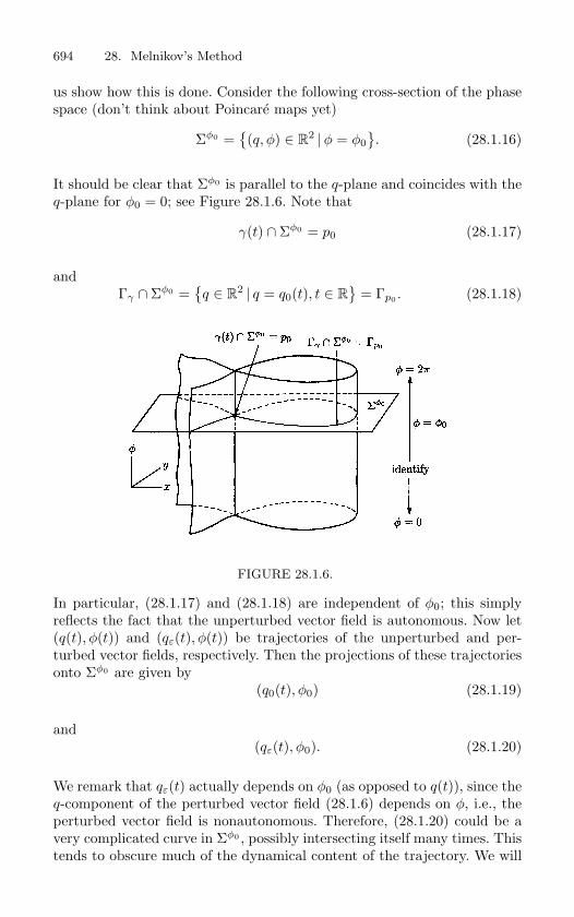
694 28. Melnikov’s Method
us show how this is done. Consider the following cross-section of the phasespace (don’t think about Poincare maps yet)
Σφ0 =(q, φ) ∈ R
2 |φ = φ0. (28.1.16)
It should be clear that Σφ0 is parallel to the q-plane and coincides with theq-plane for φ0 = 0; see Figure 28.1.6. Note that
γ(t) ∩ Σφ0 = p0 (28.1.17)
andΓγ ∩ Σφ0 =
q ∈ R
2 | q = q0(t), t ∈ R
= Γp0 . (28.1.18)
FIGURE 28.1.6.
In particular, (28.1.17) and (28.1.18) are independent of φ0; this simplyreflects the fact that the unperturbed vector field is autonomous. Now let(q(t), φ(t)) and (qε(t), φ(t)) be trajectories of the unperturbed and per-turbed vector fields, respectively. Then the projections of these trajectoriesonto Σφ0 are given by
(q0(t), φ0) (28.1.19)
and(qε(t), φ0). (28.1.20)
We remark that qε(t) actually depends on φ0 (as opposed to q(t)), since theq-component of the perturbed vector field (28.1.6) depends on φ, i.e., theperturbed vector field is nonautonomous. Therefore, (28.1.20) could be avery complicated curve in Σφ0 , possibly intersecting itself many times. Thistends to obscure much of the dynamical content of the trajectory. We will
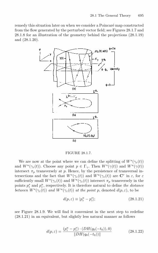
28.1 The General Theory 695
remedy this situation later on when we consider a Poincare map constructedfrom the flow generated by the perturbed vector field; see Figures 28.1.7 and28.1.8 for an illustration of the geometry behind the projections (28.1.19)and (28.1.20).
FIGURE 28.1.7.
We are now at the point where we can define the splitting of W s(γε(t))and Wu(γε(t)). Choose any point p ∈ Γγ . Then W s(γ(t)) and Wu(γ(t))intersect πp transversely at p. Hence, by the persistence of transversal in-tersections and the fact that W s(γε(t)) and Wu(γε(t)) are Cr in ε, for εsufficiently small W s(γε(t)) and Wu(γε(t)) intersect πp transversely in thepoints ps
ε and puε , respectively. It is therefore natural to define the distance
between W s(γε(t)) and Wu(γε(t)) at the point p, denoted d(p, ε), to be
d(p, ε) ≡ |puε − ps
ε|; (28.1.21)
see Figure 28.1.9. We will find it convenient in the next step to redefine(28.1.21) in an equivalent, but slightly less natural manner as follows
d(p, ε) =(pu
ε − psε) · (DH(q0(−t0)), 0)‖DH(q0(−t0))‖
(28.1.22)
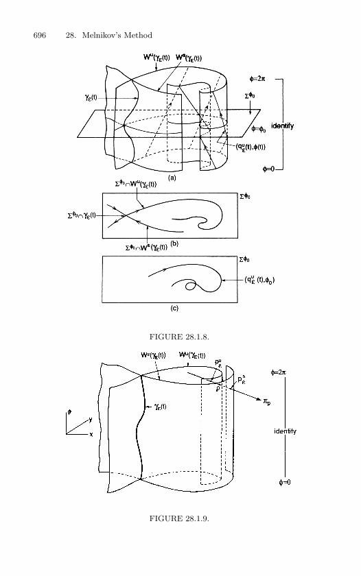
696 28. Melnikov’s Method
FIGURE 28.1.8.
FIGURE 28.1.9.
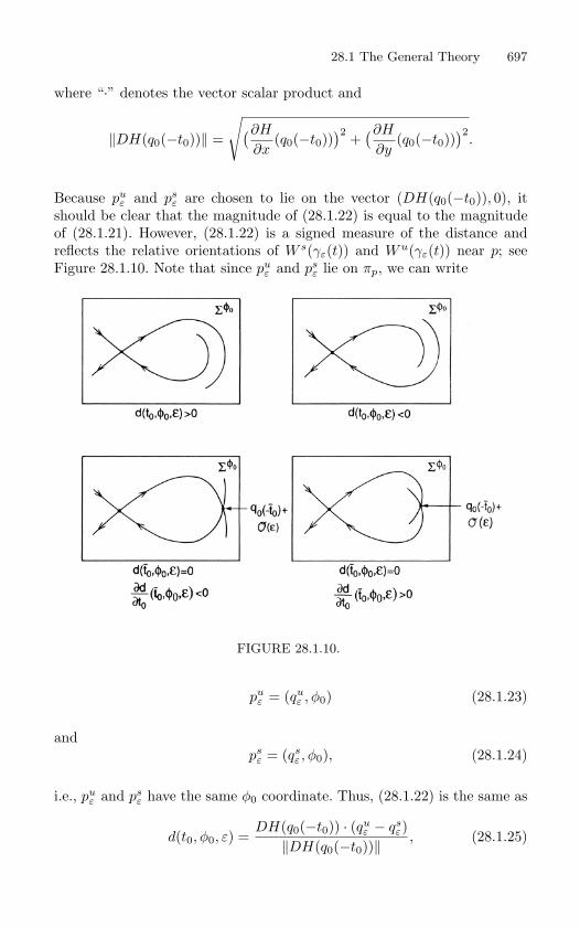
28.1 The General Theory 697
where “·” denotes the vector scalar product and
‖DH(q0(−t0))‖ =
√(∂H
∂x(q0(−t0))
)2 +(∂H
∂y(q0(−t0))
)2.
Because puε and ps
ε are chosen to lie on the vector (DH(q0(−t0)), 0), itshould be clear that the magnitude of (28.1.22) is equal to the magnitudeof (28.1.21). However, (28.1.22) is a signed measure of the distance andreflects the relative orientations of W s(γε(t)) and Wu(γε(t)) near p; seeFigure 28.1.10. Note that since pu
ε and psε lie on πp, we can write
FIGURE 28.1.10.
puε = (qu
ε , φ0) (28.1.23)
andps
ε = (qsε , φ0), (28.1.24)
i.e., puε and ps
ε have the same φ0 coordinate. Thus, (28.1.22) is the same as
d(t0, φ0, ε) =DH(q0(−t0)) · (qu
ε − qsε)
‖DH(q0(−t0))‖, (28.1.25)
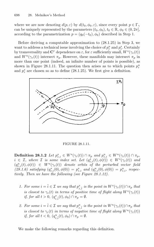
698 28. Melnikov’s Method
where we are now denoting d(p, ε) by d(t0, φ0, ε), since every point p ∈ Γγ
can be uniquely represented by the parameters (t0, φ0), t0 ∈ R, φ0 ∈ (0, 2π],according to the parametrization p = (q0(−t0), φ0) described in Step 1.
Before deriving a computable approximation to (28.1.25) in Step 3, wewant to address a technical issue involving the choice of pu
ε and psε. Certainly
by transversality and Cr dependence on ε, for ε sufficiently small, W s(γε(t))and Wu(γε(t)) intersect πp. However, these manifolds may intersect πp inmore than one point (indeed, an infinite number of points is possible), asshown in Figure 28.1.11. The question then arises as to which points pu
ε
and psε are chosen so as to define (28.1.25). We first give a definition.
FIGURE 28.1.11.
Definition 28.1.2 Let psε,i ∈ W s(γε(t)) ∩ πp and pu
ε,i ∈ Wu(γε(t)) ∩ πp,
i ∈ I, where I is some index set. Let (qsε,i(t), φ(t)) ∈ W s(γε(t)) and
(quε,i(t), φ(t)) ∈ Wu(γε(t)) denote orbits of the perturbed vector field
(28.1.6) satisfying (qsε,i(0), φ(0)) = ps
ε,i and (quε,i(0), φ(0)) = pu
ε,i, respec-
tively. Then we have the following (see Figure 28.1.12).
1. For some i = i ∈ I we say that psε,i
is the point in W s(γε(t))∩πp that
is closest to γε(t) in terms of positive time of flight along W s(γε(t))if, for all t > 0, (qs
ε,i(t), φ0) ∩ πp = ∅.
2. For some i = i ∈ I we say that puε,i
is the point in Wu(γε(t))∩πp that
is closest to γε(t) in terms of negative time of flight along Wu(γε(t))if, for all t < 0, (qu
ε,i(t), φ0) ∩ πp = ∅.
We make the following remarks regarding this definition.
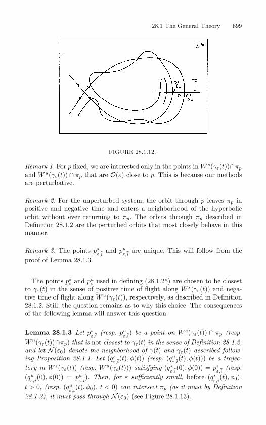
28.1 The General Theory 699
FIGURE 28.1.12.
Remark 1. For p fixed, we are interested only in the points in W s(γε(t))∩πp
and Wu(γε(t)) ∩ πp that are O(ε) close to p. This is because our methodsare perturbative.
Remark 2. For the unperturbed system, the orbit through p leaves πp inpositive and negative time and enters a neighborhood of the hyperbolicorbit without ever returning to πp. The orbits through πp described inDefinition 28.1.2 are the perturbed orbits that most closely behave in thismanner.
Remark 3. The points psε,i
and puε,i
are unique. This will follow from theproof of Lemma 28.1.3.
The points psε and pu
ε used in defining (28.1.25) are chosen to be closestto γε(t) in the sense of positive time of flight along W s(γε(t)) and nega-tive time of flight along Wu(γε(t)), respectively, as described in Definition28.1.2. Still, the question remains as to why this choice. The consequencesof the following lemma will answer this question.
Lemma 28.1.3 Let psε,i
(resp. puε,i
) be a point on W s(γε(t)) ∩ πp (resp.
Wu(γε(t))∩πp) that is not closest to γε(t) in the sense of Definition 28.1.2,
and let N (ε0) denote the neighborhood of γ(t) and γε(t) described follow-
ing Proposition 28.1.1. Let (qsε,i
(t), φ(t)) (resp. (quε,i
(t), φ(t))) be a trajec-
tory in W s(γε(t)) (resp. Wu(γε(t))) satisfying (qsε,i
(0), φ(0)) = psε,i
(resp.
(quε,i
(0), φ(0)) = puε,i
). Then, for ε sufficiently small, before (qsε,i
(t), φ0),t > 0, (resp. (qu
ε,i(t), φ0), t < 0) can intersect πp (as it must by Definition
28.1.2), it must pass through N (ε0) (see Figure 28.1.13).
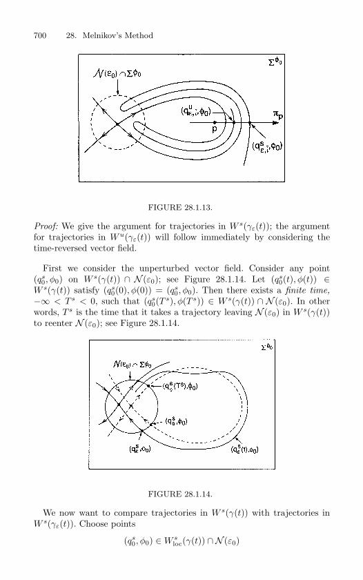
700 28. Melnikov’s Method
FIGURE 28.1.13.
Proof: We give the argument for trajectories in W s(γε(t)); the argumentfor trajectories in Wu(γε(t)) will follow immediately by considering thetime-reversed vector field.
First we consider the unperturbed vector field. Consider any point(qs
0, φ0) on W s(γ(t)) ∩ N (ε0); see Figure 28.1.14. Let (qs0(t), φ(t)) ∈
W s(γ(t)) satisfy (qs0(0), φ(0)) = (qs
0, φ0). Then there exists a finite time,
−∞ < T s < 0, such that (qs0(T
s), φ(T s)) ∈ W s(γ(t)) ∩ N (ε0). In otherwords, T s is the time that it takes a trajectory leaving N (ε0) in W s(γ(t))to reenter N (ε0); see Figure 28.1.14.
FIGURE 28.1.14.
We now want to compare trajectories in W s(γ(t)) with trajectories inW s(γε(t)). Choose points
(qs0, φ0) ∈ W s
loc(γ(t)) ∩N (ε0)
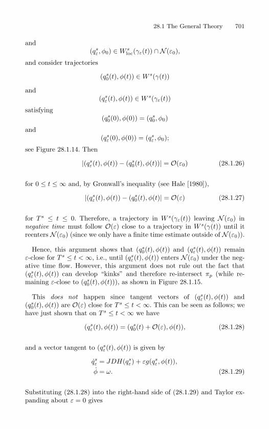
28.1 The General Theory 701
and(qs
ε , φ0) ∈ W sloc(γε(t)) ∩N (ε0),
and consider trajectories
(qs0(t), φ(t)) ∈ W s(γ(t))
and(qs
ε(t), φ(t)) ∈ W s(γε(t))
satisfying(qs
0(0), φ(0)) = (qs0, φ0)
and(qs
ε(0), φ(0)) = (qsε , φ0);
see Figure 28.1.14. Then
|(qsε(t), φ(t))− (qs
0(t), φ(t))| = O(ε0) (28.1.26)
for 0 ≤ t ≤ ∞ and, by Gronwall’s inequality (see Hale [1980]),
|(qsε(t), φ(t))− (qs
0(t), φ(t)| = O(ε) (28.1.27)
for T s ≤ t ≤ 0. Therefore, a trajectory in W s(γε(t)) leaving N (ε0) innegative time must follow O(ε) close to a trajectory in W s(γ(t)) until itreenters N (ε0) (since we only have a finite time estimate outside of N (ε0)).
Hence, this argument shows that (qs0(t), φ(t)) and (qs
ε(t), φ(t)) remainε-close for T s ≤ t < ∞, i.e., until (qs
ε(t), φ(t)) enters N (ε0) under the neg-ative time flow. However, this argument does not rule out the fact that(qs
ε(t), φ(t)) can develop “kinks” and therefore re-intersect πp (while re-maining ε-close to (qs
0(t), φ(t))), as shown in Figure 28.1.15.
This does not happen since tangent vectors of (qsε(t), φ(t)) and
(qs0(t), φ(t)) are O(ε) close for T s ≤ t < ∞. This can be seen as follows; we
have just shown that on T s ≤ t < ∞ we have
(qsε(t), φ(t)) = (qs
0(t) +O(ε), φ(t)), (28.1.28)
and a vector tangent to (qsε(t), φ(t)) is given by
qsε = JDH(qs
ε) + εg(qsε , φ(t)),
φ = ω. (28.1.29)
Substituting (28.1.28) into the right-hand side of (28.1.29) and Taylor ex-panding about ε = 0 gives
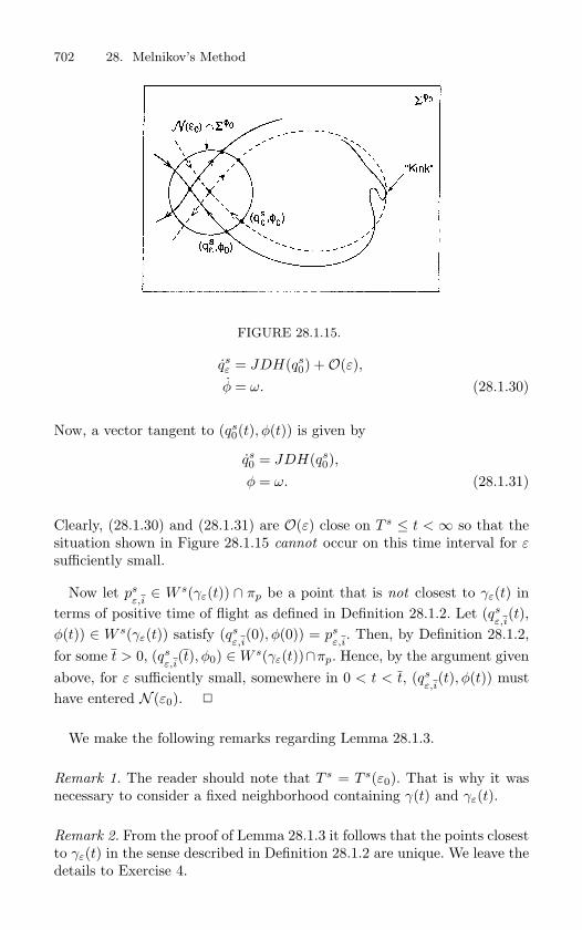
702 28. Melnikov’s Method
FIGURE 28.1.15.
qsε = JDH(qs
0) +O(ε),φ = ω. (28.1.30)
Now, a vector tangent to (qs0(t), φ(t)) is given by
qs0 = JDH(qs
0),φ = ω. (28.1.31)
Clearly, (28.1.30) and (28.1.31) are O(ε) close on T s ≤ t < ∞ so that thesituation shown in Figure 28.1.15 cannot occur on this time interval for εsufficiently small.
Now let psε,i∈ W s(γε(t)) ∩ πp be a point that is not closest to γε(t) in
terms of positive time of flight as defined in Definition 28.1.2. Let (qsε,i
(t),φ(t)) ∈ W s(γε(t)) satisfy (qs
ε,i(0), φ(0)) = ps
ε,i. Then, by Definition 28.1.2,
for some t > 0, (qsε,i
(t), φ0) ∈ W s(γε(t))∩πp. Hence, by the argument givenabove, for ε sufficiently small, somewhere in 0 < t < t, (qs
ε,i(t), φ(t)) must
have entered N (ε0).
We make the following remarks regarding Lemma 28.1.3.
Remark 1. The reader should note that T s = T s(ε0). That is why it wasnecessary to consider a fixed neighborhood containing γ(t) and γε(t).
Remark 2. From the proof of Lemma 28.1.3 it follows that the points closestto γε(t) in the sense described in Definition 28.1.2 are unique. We leave thedetails to Exercise 4.
28.1 The General Theory 703
Remark 3. Let psε = (qs
ε , φ0) ∈ W s(γε(t)) ∩ πp, and let (qsε(t), φ(t)) ∈
W s(γε(t)) satisfy (qsε(0), φ(0)) = (qs
ε , φ0). Then if psε is the point closest to
γε(t) in the sense of Definition 28.1.2, it follows from the proof of Lemma28.1.3 that
|qsε(t)− q0(t− t0)| = O(ε), t ∈ [0,∞), (28.1.32)
|qsε(t)− q0(t− t0)| = O(ε), t ∈ [0,∞). (28.1.33)
A similar statement can be made for points in Wu(γε(t)) ∩ πp and solu-tions in Wu(γε(t)). In deriving the Melnikov function in the next step wewill need to approximate perturbed solutions in W s(γε(t)) and Wu(γε(t))by unperturbed solutions in W s(γ(t)) and Wu(γ(t)) for semi-infinite timeintervals with O(ε) accuracy. This is why the Melnikov function will onlydetect points on W s(γε(t))∩πp ∩Wu(γε(t)) that are closest to γε(t) in thesense of Definition 28.1.2.
Step 3: Derivation of the Melnikov Function. Taylor expanding (28.1.25)about ε = 0 gives
d(t0, φ0, ε) = d(t0, φ0, 0) + ε∂d
∂ε(t0, φ0, 0) +O(ε2), (28.1.34)
whered(t0, φ0, 0) = 0 (28.1.35)
and]
∂d
∂ε(t0, φ0, 0) =
DH(q0(−t0)) ·(∂qu
ε
∂ε |ε=0 − ∂qsε
∂ε |ε=0)‖DH(q0(−t0))‖
. (28.1.36)
The Melnikov function is defined to be
M(t0, φ0) ≡ DH(q0(−t0)) ·(
∂quε
∂ε
∣∣∣∣ε=0
− ∂qsε
∂ε
∣∣∣∣ε=0
). (28.1.37)
Now, since
DH(q0(−t0)) =(
∂H
∂x(q0(−t0)),
∂H
∂y(q0(−t0))
)
is not zero on q0(−t0), for t0 finite, we see that
704 28. Melnikov’s Method
M(t0, φ0) = 0 ⇒ ∂d
∂ε(t0, φ0) = 0. (28.1.38)
Therefore, up to a nonzero normalization factor (‖DH(q0(−t0))‖), the Mel-nikov function is the lowest order nonzero term in the Taylor expansion forthe distance between W s(γε(t)) and Wu(γε(t)) at the point p.
We now want to derive an expression for M(t0, φ0) that can be computedwithout needing to know the solution of the perturbed vector field. Wedo this by utilizing Melnikov’s original trick. We define a time-dependentMelnikov function using the flow generated by both the unperturbed vectorfield and the perturbed vector field. We have to be careful here since wedo not have any a priori knowledge of arbitrary orbits generated by theperturbed vector field. However, the persistence and differentiability of γ(t),W s(γ(t)), and Wu(γ(t)) as described in Proposition 28.1.1 are all that weneed, since Definition 28.1.2 and Lemma 28.1.3 allow us to characterize theorbits of interest for determining the splitting of W s(γε(t)) and Wu(γε(t)).We then derive an ordinary differential equation which the time-dependentMelnikov function must satisfy. The ordinary differential equation turnsout to be first order and linear; hence it is trivially solvable. The solutionevaluated at the appropriate time will yield the Melnikov function.
We begin by defining the time-dependent Melnikov function as follows
M(t; t0, φ0) ≡ DH(q0(t− t0)) ·(
∂quε (t)∂ε
∣∣∣∣ε=0
− ∂qsε(t)∂ε
∣∣∣∣ε=0
). (28.1.39)
We want to take some care in describing precisely what we mean by(28.1.39). We denote orbits in W s(γε(t)) and Wu(γε(t)) by qs
ε(t) and quε (t),
respectively. Then in (28.1.39) the expressions
∂quε (t)∂ε
∣∣∣∣ε=0
(28.1.40)
and∂qs
ε(t)∂ε
∣∣∣∣ε=0
(28.1.41)
are simply the derivatives with respect to ε (evaluated at ε = 0) of quε (t)
and qsε(t), respectively, where qu
ε (t) and qsε(t) satisfy
quε (0) = qu
ε , (28.1.42)
qsε(0) = qs
ε . (28.1.43)
28.1 The General Theory 705
The expression q0(t− t0) denotes the unperturbed homoclinic orbit. Thus,we see that (28.1.39) is a bit unusual; part of it, (DH(q0(t−t0))), evolves intime under the dynamics of the unperturbed vector field with the remainingpart (
∂quε (t)∂ε
∣∣∣∣ε=0
− ∂qsε(t)∂ε
∣∣∣∣ε=0
)
evolving in time under the dynamics of the perturbed vector field. It shouldbe obvious that the relationship between the time-dependent Melnikovfunction and the Melnikov function is given by
M(0; t0, φ0) = M(t0, φ0). (28.1.44)
Next we turn to deriving an ordinary differential equation thatM(t; t0, φ0) must satisfy. The expressions we derive will be a bit cumber-some, so for the sake of a more compact notation we define
∂quε (t)∂ε
∣∣∣∣ε=0
≡ qu1 (t),
∂qsε(t)∂ε
∣∣∣∣ε=0
≡ qs1(t).
Then (28.1.39) can be rewritten as
M(t; t0, φ0) = DH(q0(t− t0)) · (qu1 (t)− qs
1(t)). (28.1.45)
We want to introduce a further definition to compactify the notation asfollows
M(t; t0, φ0) ≡ ∆u(t)−∆s(t), (28.1.46)
where∆u,s(t) ≡ DH(q0(t− t0)) · qu,s
1 (t). (28.1.47)
Differentiating (28.1.47) with respect to t gives
d
dt(∆u,s(t)) =
(d
dt(DH(q0(t− t0)))
)· qu,s
1 (t)
+ DH(q0(t− t0)) ·d
dtqu,s1 (t). (28.1.48)
The term ddt (q
u,s1 (t)) in (28.1.48) needs some explanation. Recall from above
that we have defined
706 28. Melnikov’s Method
qu,s1 (t) ≡ ∂qu,s
ε (t)∂ε
∣∣∣∣ε=0
,
and qu,sε (t) solves
d
dt(qu,s
ε (t)) = JDH(qu,sε (t)) + εg(qu,s
ε (t), φ(t), ε), (28.1.49)
where φ(t) = ωt + φ0. Since qu,sε (t) is Cr in ε and t (see Theorem 7.3.1),
we can differentiate (28.1.49) with respect to ε and interchange the orderof the ε and t differentiations to obtain
d
dt
(∂qu,s
ε (t)∂ε
∣∣∣∣ε=0
)= JD2H(q0(t− t0))
∂qu,sε (t)∂ε
∣∣∣∣ε=0(t)
+ g(q0(t− t0), φ(t), 0) (28.1.50)
or
d
dtqu,s1 (t) = JD2H(q0(t− t0))q
u,s1 (t) + g(q0(t− t0), φ(t), 0). (28.1.51)
Equation (28.1.51) is referred to as the first variational equation. We remarkthat qu
1 (t) solves (28.1.51) for t ∈ (−∞, 0], and qs1(t) solves (4.5.51) for
t ∈ (0,∞]; see the remarks following Lemma 28.1.3. Substituting (28.1.51)into (28.1.48) gives
d
dt(∆u,s(t)) =
(d
dt(DH(q0(t− t0)))
)· qu,s
1 (t)
+ DH(q0(t− t0)) · JD2H(q0(t− t0))qu,s1 (t)
+ DH(q0(t− t0)) · g(q0(t− t0), φ(t), 0). (28.1.52)
Now a wonderful thing happens.
Lemma 28.1.4(d
dt(DH(q0(t− t0)))
)· qu,s
1 (t)
+ DH(q0(t− t0)) · JD2H(q0(t− t0))qu,s1 (t) = 0.
Proof: First note that
28.1 The General Theory 707
d
dt
(DH(q0(t− t0))
)= D2H(q0(t− t0))q0(t− t0)
=(D2H(q0(t− t0))
)(JDH(q0(t− t0))
).
(28.1.53)
Let qu,s1 (t) = (xu,s
1 (t), yu,s1 (t)). Then we have
(D2H)(JDH) · qu,s1 =
(∂2H∂x2
∂2H∂x∂y
∂2H∂x∂y
∂2H∂y2
)( ∂H∂y
−∂H∂x
)·
xu,s
1
yu,s1
= xu,s1
[∂2H
∂x2
∂H
∂y− ∂2H
∂x∂y
∂H
∂x
]
+ yu,s1
[∂2H
∂x∂y
∂H
∂y− ∂2H
∂y2
∂H
∂x
](28.1.54)
and
DH · (JD2H)qu,s1 =
( ∂H∂x∂H∂y
)·(
∂2H∂x∂y
∂2H∂y2
−∂2H∂x2
∂2H∂x∂y
)xu,s
1
yu,s1
= xu,s1
[∂2H
∂x∂y
∂H
∂x− ∂2H
∂x2
∂H
∂y
]
+ yu,s1
[∂2H
∂y2
∂H
∂x− ∂2H
∂x∂y
∂H
∂y
], (28.1.55)
where we have left out the argument q0(t − t0) = (x0(t − t0), y0(t − t0))for the sake of a less cumbersome notation. Adding (28.1.54) and (28.1.55)gives the result.
Therefore, using Lemma 28.1.4, (28.1.48) becomes
d
dt(∆u,s(t)) = DH(q0(t− t0)) · g(q0(t− t0), φ(t), 0). (28.1.56)
Integrating ∆u(t) and ∆s(t) individually from −τ to 0 and 0 to τ (τ > 0),respectively, gives
∆u(0)−∆u(−τ) =∫ 0
−τ
DH(q0(t−t0)) ·g(q0(t−t0), ωt+φ0, 0)dt (28.1.57)
and
708 28. Melnikov’s Method
∆s(τ)−∆s(0) =∫ τ
0DH(q0(t− t0)) · g(q0(t− t0), ωt + φ0, 0)dt (28.1.58)
where we have substituted φ(t) = ωt + φ0 into the integrand. Adding(28.1.57) and (28.1.58) and referring to (28.1.44) and (28.1.46) gives
M(t0, φ0) = M(0, t0, φ0) = ∆u(0)−∆s(0)
=∫ τ
−τ
DH(q0(t− t0)) · g(q0(t− t0), ωt + φ0, 0)dt
+∆s(τ)−∆u(−τ). (28.1.59)
We now want to consider the limit of (28.1.59) as τ →∞.
Lemma 28.1.5
limτ→∞
∆s(τ) = limτ→∞
∆u(−τ) = 0.
Proof: Recall from (28.1.47) that
∆u,s(t) = DH(q0(t− t0)) · qu,s1 (t).
Now, as t →∞ (resp. −∞), DH(q0(t− t0)) goes to zero exponentially fast,since q0(t− t0) approaches a hyperbolic fixed point. Also, as t →∞ (resp.−∞), qs
1(t) (resp. qu1 (t)) is bounded (see Exercise 6). Hence, ∆s(τ) (resp.
∆u(−τ)) goes to zero as τ →∞.
Lemma 28.1.6 The improper integral∫ ∞
−∞DH(q0(t− t0)) · g(q0(t− t0), ωt + φ0, 0)dt
converges absolutely.
Proof: This result follows from the fact that g(q0(t − t0), ωt + φ0, 0) isbounded for all t and DH(q0(t − t0)) goes to zero exponentially fast ast → ±∞.
Hence, combining Lemma 28.1.5 and Lemma 28.1.6, (28.1.59) becomes
M(t0, φ0) =∫ ∞
−∞DH(q0(t− t0)) · g(q0(t− t0), ωt + φ0, 0)dt. (28.1.60)
28.1 The General Theory 709
Before giving the main theorem we want to point out an interestingproperty of the Melnikov function. If we make the transformation
t −→ t + t0,
then (28.1.60) becomes
M(t0, φ0) =∫ ∞
−∞DH(q0(t)) · g(q0(t), ωt + ωt0 + φ0, 0)dt. (28.1.61)
Recall that g(q, ·, 0) is periodic, which implies that M(t0, φ0) is periodic int0 with period 2π/ω and periodic in φ0 with period 2π. The geometry of thiswill be explained shortly. However, it should be clear from (28.1.61) thatvarying t0 and varying φ0 have the same effect. Moreover, from (28.1.61)and the periodicity of g(q, ·, 0), it follows that
∂M
∂φ0(t0, φ0) =
1ω
∂M
∂t0(t0, φ0); (28.1.62)
hence, ∂M∂t0
= 0 if and only if ∂M∂φ0
= 0. In Theorem 28.1.7 we will need tohave ∂M
∂t0 = 0 or ∂M
∂φ0 = 0. However, from (28.1.62), if one is nonzero, then
so is the other; hence, we will state the theorem in terms of ∂M∂t0
= 0.
Theorem 28.1.7 Suppose we have a point (t0, φ0) = (t0, φ0) such that
i) M(t0, φ0) = 0 and
ii) ∂M∂t0
∣∣∣(t0,φ0)
= 0.
Then, for ε sufficiently small, W s(γε(t)) and Wu(γε(t)) intersect trans-
versely at (q0(−t0)+O(ε), φ0). Moreover, if M(t0, φ0) = 0 for all (t0, φ0) ∈R
1 × S1, then W s(γε(t)) ∩Wu(γε(t)) = ∅.
Proof: Recall from (28.1.34), (28.1.36), and (28.1.37) that we have
d(t0, φ0, ε) = εM(t0, φ0)
‖DH(q0(−t0))‖+O(ε2). (28.1.63)
Note that if we define
d(t0, φ0, ε) = εd(t0, φ0, ε), (28.1.64)
where
710 28. Melnikov’s Method
d(t0, φ0, ε) =M(t0, φ0)
‖DH(q0(−t0))‖+O(ε), (28.1.65)
thend(t0, φ0, ε) = 0 ⇒ d(t0, φ0, ε) = 0. (28.1.66)
Therefore, we will work with d(t0, φ0, ε).
Now at (t0, φ0, ε) = (t0, φ0, 0) we have
d(t0, φ0, 0) =M(t0, φ0)
‖DH(q0(−t0))‖= 0, (28.1.67)
with
∂d
∂t0
∣∣∣∣∣(t0,φ0,0)
=1
‖DH(q0(−t0))‖∂M
∂t0
∣∣∣∣(t0,φ0)
= 0. (28.1.68)
By the implicit function theorem, there thus exists a function
t0 = t0(φ0, ε) (28.1.69)
for |φ− φ0|, ε sufficiently small, such that
d(t0(φ0, ε), φ0, ε) = 0. (28.1.70)
This shows that W s(γε(t)) and Wu(γε(t)) intersect O(ε) close to(q0(−t0), φ0). Next we need to worry about transversality.
Suppose that W s(γε(t)) and Wu(γε(t)) intersect at some point p. Thenrecall from Chapter 12 that the intersection is said to be transversal if
TpWs(γε(t)) + TpW
u(γε(t)) = R3. (28.1.71)
Now, for ε sufficiently small, the points on W s(γε(t)) and Wu(γε(t)) thatare closest to γε(t) in the sense of Definition 28.1.2 can be parametrized byt0 and φ0. Hence, (
∂quε
∂t0,∂qu
ε
∂φ0
)(28.1.72)
and (∂qs
ε
∂t0,∂qs
ε
∂φ0
)(28.1.73)
are a basis for TpWu(γε(t)) and TpW
s(γε(t)), respectively.
(Note: it is important for the reader to understand how (28.1.72) and(28.1.73) are computed. By definition, p = (qs
ε , φ0) = (quε , φ0), and qs
ε andquε are the points satisfying qs
ε(0) = qsε , qu
ε (0) = quε , where qs
ε(t) and quε (t)
28.2 Poincare Maps and the Geometry of the Melnikov Function 711
are trajectories in W s(γε(t)) and Wu(γε(t)), respectively. Since those tra-jectories depend parametrically on t0 and φ0, (28.1.72) and (28.1.73) aresimply the derivatives of the respective trajectories with respect to t0 andφ0 evaluated at t = 0.)
TpWs(γε(t)) and TpW
u(γε(t)) will not be tangent at p provided
∂quε
∂t0− ∂qs
ε
∂t0 = 0 (28.1.74)
or∂qu
ε
∂φ0− ∂qu
ε
∂φ0 = 0. (28.1.75)
Differentiating d(t0, φ0, ε) with respect to t0 and φ0 and evaluating at theintersection point given by (t0 +O(ε), φ0) (where M(t0, φ0) = 0) gives
∂d
∂t0(t0, φ0, ε) =
DH(q0(−t0)) · ((∂quε )/(∂t0)− (∂qs
ε)/(∂t0))‖DH(q0(−t0))‖
= ε(∂M/∂t0)(t0, φ0)‖DH(q0(−t0))‖
+O(ε2), (28.1.76)
∂d
∂φ0(t0, φ0, ε) =
DH(q0(−t0)) · ((∂quε )/(∂φ0)− (∂qs
ε)/(∂φ0))‖DH(q0(−t0))‖
= ε(∂M/∂φ0)(t0, φ0)‖DH(q0(−t0))‖
+O(ε2). (28.1.77)
Hence, it should be clear from (28.1.76) and (28.1.77) that, for ε sufficientlysmall, a sufficient condition for transversality is
∂M
∂φ0(t0, φ0) =
1ω
∂M
∂t0(t0, φ0) = 0. (28.1.78)
Finally, we leave the fact that M(t0, φ0) = 0 implies W s(γε(t))∩Wu(γε(t)) = ∅ as an exercise for the reader (see Exercise 7).
28.2 Poincare Maps and the Geometry of theMelnikov Function
We now want to describe the geometry associated with the independentvariables, t0 and φ0, of the Melnikov function.
Consider the following cross-section to the phase space R2 × S1
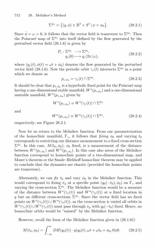
712 28. Melnikov’s Method
Σφ0 =(q, φ) ∈ R
2 × S1 |φ = φ0. (28.2.1)
Since φ = ω > 0, it follows that the vector field is transverse to Σφ0 . Thenthe Poincare map of Σφ0 into itself defined by the flow generated by theperturbed vector field (28.1.6) is given by
Pε : Σφ0 −→ Σφ0 ,qε(0) −→ qε(2π/ω), (28.2.2)
where (qε(t), φ(t) = ωt + φ0) denotes the flow generated by the perturbedvector field (28.1.6). Now the periodic orbit γε(t) intersects Σφ0 in a pointwhich we denote as
pε,φ0 = γε(t) ∩ Σφ0 . (28.2.3)
It should be clear that pε,φ0 is a hyperbolic fixed point for the Poincare maphaving a one-dimensional stable manifold, W s(pε,φ0) and a one-dimensionalunstable manifold, Wu(pε,φ0) given by
W s(pε,φ0) ≡ W s(γε(t)) ∩ Σφ0
andWu(pε,φ0) ≡ Wu(γε(t)) ∩ Σφ0 , (28.2.4)
respectively; see Figure 28.2.1.
Now let us return to the Melnikov function. From our parametrizationof the homoclinic manifold, Γγ , it follows that fixing φ0 and varying t0corresponds to restricting our distance measurement to a fixed cross-sectionΣφ0 . In this case, M(t0, φ0), φ0 fixed, is a measurement of the distancebetween W s(pε,φ0) and Wu(pε,φ0). In this case also zeros of the Melnikovfunction correspond to homoclinic points of a two-dimensional map, andMoser’s theorem or the Smale–Birkhoff homoclinic theorem may be appliedto conclude that the dynamics are chaotic (provided the homoclinic pointsare transverse).
Alternately, we can fix t0 and vary φ0 in the Melnikov function. Thiswould correspond to fixing πp at a specific point (q0(−t0), φ0) on Γγ andvarying the cross-section Σφ0 . The Melnikov function would be a measureof the distance between W s(γε(t)) and Wu(γε(t)) at a fixed location inq but on different cross-sections Σφ0 . Since the vector field has no fixedpoints on W s(γε(t))∪Wu(γε(t)), as the cross-section is varied all orbits inW s(γε(t))∪Wu(γε(t)) must pass through πp with q0(−t0) fixed. Hence, nohomoclinic orbits would be “missed” by the Melnikov function.
However, recall the form of the Melnikov function given in (28.1.61)
M(t0, φ0) =∫ ∞
−∞DH(q0(t)) · g(q0(t), ωt + ωt0 + φ0, 0)dt. (28.2.5)
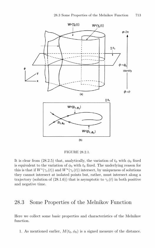
28.3 Some Properties of the Melnikov Function 713
FIGURE 28.2.1.
It is clear from (28.2.5) that, analytically, the variation of t0 with φ0 fixedis equivalent to the variation of φ0 with t0 fixed. The underlying reason forthis is that if W s(γε(t)) and Wu(γε(t)) intersect, by uniqueness of solutionsthey cannot intersect at isolated points but, rather, must intersect along atrajectory (solution of (28.1.6)) that is asymptotic to γε(t) in both positiveand negative time.
28.3 Some Properties of the Melnikov Function
Here we collect some basic properties and characteristics of the Melnikovfunction.
1. As mentioned earlier, M(t0, φ0) is a signed measure of the distance.
714 28. Melnikov’s Method
We now want to explore this in more detail. Let us restrict ourselvesto the Poincare map defined on the cross-section Σφ0 and view φ0as fixed; then d(t0, φ0, ε) measures the distance between W s(pε,φ0)and Wu(pε,φ0) (see Section 28.2). We recall that the distance between
W s(pε,φ0) and Wu(pε,φ0) at the point p = (q0(−t0), φ0) is given by
d(t0, φ0, ε) =DH(q0(−t0)) · (qu
ε − qsε)
‖DH(q0(−t0))‖
= εM(t0, φ0)
‖DH(q0(−t0))‖+O(ε2) (28.3.1)
where quε and qs
ε are defined in Definition 28.1.2. Hence, for ε suffi-ciently small
M(t0, φ0)> 0< 0
⇒ d(t0, φ0, ε)> 0< 0
. (28.3.2)
Thus, using (28.3.1) and (28.3.2), Figure 28.1.10 holds if we replaced(t0, φ0, ε) with M(t0, φ0).
2. M(t0, φ0) is periodic in t0 with period 2π/ω and periodic in φ0 withperiod 2π. This follows from the fact that the perturbation, εg(q, t, ε),is periodic in t with period 2π/ω as well as from the form of M(t0, φ0)given in (28.1.61).
3. Recall from (28.3.1) that the distance between W s(γε(t)) andWu(γε(t)) is given by
d(t0, φ0, ε) = εM(t0, φ0)
‖DH(q0(−t0))‖+O(ε2). (28.3.3)
We want to focus on the denominator, ‖DH(q0(−t0))‖, in the O(ε)term of (28.3.3). Let us consider the situation with φ0 fixed so thatd(t0, φ0, ε) measures the distance between the stable and unstablemanifolds of a hyperbolic fixed point of the Poincare map (see Sec-tion 28.2). Then, as t0 → ±∞, the measurement of distance is beingmade close to the hyperbolic fixed point (since q0(−t0) approaches theunperturbed hyperbolic fixed point as t0 → ±∞). Also, as t0 → ±∞,‖DH(q0(−t0))‖ → 0, indicating that d(t0, φ0, ε) →∞. Geometrically,this means that the distance between the manifolds is oscillating un-boundedly near the hyperbolic fixed point. The reader should com-pare this analytic result with the geometrical picture given by thelambda lemma (Lemma 26.0.4).
4. Suppose that the perturbation is autonomous, i.e., εg(q) does notdepend explicitly on time. Then the Melnikov function is given by
M =∫ ∞
−∞DH(q0(t)) · g(q0(t), 0)dt. (28.3.4)
28.4 Homoclinic Bifurcations 715
In this case M is just a number, i.e., it is not a function of t0 andφ0. This makes sense, since, for autonomous two-dimensional vectorfields, either the stable and unstable manifolds of a hyperbolic fixedpoint coincide or they do not intersect at all. In Exercise 11 we willdeal more fully with the geometry of the Melnikov function for au-tonomous problems.
5. Suppose the vector field is Hamiltonian, i.e., we have a Cr+1 (r ≥ 2)function periodic in t with period T = 2π/ω given by
Hε(x, y, t) = H(x, y) + εH1(x, y, t, ε) (28.3.5)
such that the perturbed vector field (28.1.1) is given by
x =∂H
∂y(x, y) + ε
∂H1
∂y(x, y, t, ε),
y = −∂H
∂x(x, y)− ε
∂H1
∂x(x, y, t, ε). (28.3.6)
In this case, using (28.1.61) and (28.3.6), it is easy to see that theMelnikov function is given by
M(t0, φ0) = −∫ ∞
−∞H,H1(q0(t), ωt + ωt0 + φ0, 0)dt, (28.3.7)
whereH,H1 ≡
∂H
∂x
∂H1
∂y− ∂H
∂y
∂H1
∂x(28.3.8)
is the Poisson bracket of H with H1.
28.4 Homoclinic Bifurcations
Suppose the vector field (28.1.6) depends on a scalar parameter µ, i.e.,
q = JDH(q) + εg(q, φ, µ, ε),φ = ω, (q, φ, µ) ∈ R
2 × S1 × R1. (28.4.1)
If, in a specific problem, there is more than one parameter, then considerall but one as fixed. In this case the Melnikov functions depend on theparameter µ. In particular, we write
M(t0, φ0, µ). (28.4.2)
We will consider φ0 as fixed, i.e., the Poincare map associated with (28.4.1)is defined on the cross-section Σφ0 . We have the following bifurcation the-orem for the Melnikov function.
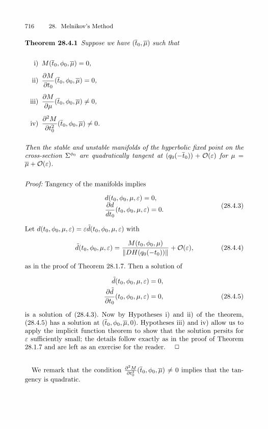
716 28. Melnikov’s Method
Theorem 28.4.1 Suppose we have (t0, µ) such that
i) M(t0, φ0, µ) = 0,
ii)∂M
∂t0(t0, φ0, µ) = 0,
iii)∂M
∂µ(t0, φ0, µ) = 0,
iv)∂2M
∂t20(t0, φ0, µ) = 0.
Then the stable and unstable manifolds of the hyperbolic fixed point on the
cross-section Σφ0 are quadratically tangent at (q0(−t0)) + O(ε) for µ =µ +O(ε).
Proof: Tangency of the manifolds implies
d(t0, φ0, µ, ε) = 0,∂d
dt0(t0, φ0, µ, ε) = 0. (28.4.3)
Let d(t0, φ0, µ, ε) = εd(t0, φ0, µ, ε) with
d(t0, φ0, µ, ε) =M(t0, φ0, µ)
‖DH(q0(−t0))‖+O(ε), (28.4.4)
as in the proof of Theorem 28.1.7. Then a solution of
d(t0, φ0, µ, ε) = 0,
∂d
∂t0(t0, φ0, µ, ε) = 0, (28.4.5)
is a solution of (28.4.3). Now by Hypotheses i) and ii) of the theorem,(28.4.5) has a solution at (t0, φ0, µ, 0). Hypotheses iii) and iv) allow us toapply the implicit function theorem to show that the solution persits forε sufficiently small; the details follow exactly as in the proof of Theorem28.1.7 and are left as an exercise for the reader.
We remark that the condition ∂2M∂t20
(t0, φ0, µ) = 0 implies that the tan-gency is quadratic.
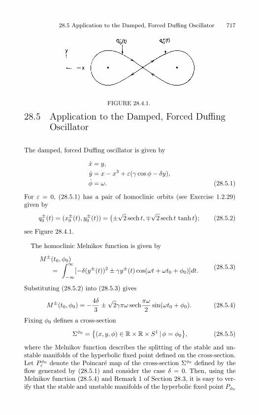
28.5 Application to the Damped, Forced Duffing Oscillator 717
FIGURE 28.4.1.
28.5 Application to the Damped, Forced DuffingOscillator
The damped, forced Duffing oscillator is given by
x = y,
y = x− x3 + ε(γ cos φ− δy),φ = ω. (28.5.1)
For ε = 0, (28.5.1) has a pair of homoclinic orbits (see Exercise 1.2.29)given by
q±0 (t) = (x±
0 (t), y±0 (t)) =
(±√
2 sech t,∓√
2 sech t tanh t); (28.5.2)
see Figure 28.4.1.
The homoclinic Melnikov function is given by
M±(t0, φ0)
=∫ ∞
−∞[−δ(y±(t))2 ± γy±(t) cos(ωt + ωt0 + φ0)]dt.
(28.5.3)
Substituting (28.5.2) into (28.5.3) gives
M±(t0, φ0) = −4δ
3±√
2γπω sechπω
2sin(ωt0 + φ0). (28.5.4)
Fixing φ0 defines a cross-section
Σφ0 =(x, y, φ) ∈ R× R× S1 |φ = φ0
, (28.5.5)
where the Melnikov function describes the splitting of the stable and un-stable manifolds of the hyperbolic fixed point defined on the cross-section.Let Pφ0
ε denote the Poincare map of the cross-section Σφ0 defined by theflow generated by (28.5.1) and consider the case δ = 0. Then, using theMelnikov function (28.5.4) and Remark 1 of Section 28.3, it is easy to ver-ify that the stable and unstable manifolds of the hyperbolic fixed point Pφ0
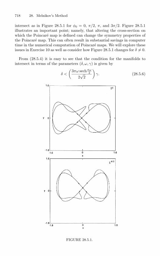
718 28. Melnikov’s Method
intersect as in Figure 28.5.1 for φ0 = 0, π/2, π, and 3π/2. Figure 28.5.1illustrates an important point; namely, that altering the cross-section onwhich the Poincare map is defined can change the symmetry properties ofthe Poincare map. This can often result in substantial savings in computertime in the numerical computation of Poincare maps. We will explore theseissues in Exercise 10 as well as consider how Figure 28.5.1 changes for δ = 0.
From (28.5.4) it is easy to see that the condition for the manifolds tointersect in terms of the parameters (δ, ω, γ) is given by
δ <
(3πω sechπω
2
2√
2
)γ. (28.5.6)
FIGURE 28.5.1.
28.5 Application to the Damped, Forced Duffing Oscillator 719
In Figure 28.5.2 we graph the critical surface δ =( 3πω sech (πω/2)
2√
2
)γ, and
we note the following.
FIGURE 28.5.2. a) Graph of the critical surface δ =(
3πω sech (πω/2)2√
2
)γ. b)
Cross-section of the critical surface for γ = constant. c) Cross-section of the
critical surface for ω = constant. d) Cross-section of the critical surface for δ =
constant.
1. The condition (28.5.6) for intersection of the manifolds is independentof the particular cross-section Σφ0 (as it should be).
2. If the “right-hand” branches of the stable and unstable manifoldsintersect, then the “left-hand” branches also intersect, and vice-versa.However, as seen in Figure 28.5.1, the geometry of intersections of theright-hand branches and left-hand branches may differ.
Thus, (28.5.6) is a criterion for chaos in the damped, forced Duffingoscillator as a function of the parameters (δ, ω, γ).
Finally we remark that Melnikov-type methods have been developed formulti-degree-of-freedom systems and for systems having more general timedependencies. These techniques also deal with orbits homoclinic to invari-ant sets other than periodic orbits. A complete exposition of this theorycan be found in Wiggins [1988].
720 28. Melnikov’s Method
28.6 Exercises
1. Consider the parametrization of the homoclinic manifold given in (28.1.9). Show thatthe map
(t0, φ0) → (q0(−t0), φ0), (t0, φ0) ∈ R1 × S
1,
is Cr, one-to-one, and onto.
2. Recall Proposition 28.1.1. Prove that, for ε sufficiently small, γε(t) persists as a peri-odic orbit of period T = 2π/ω having the same stability type as γ(t). For informationconcerning the persistence of the local stable and unstable manifolds, see Fenichel[1971] or Wiggins [1994].
3. Suppose that Γγ intersects πp transversely at some p = (q0(−t0), φ0). Show that,for ε sufficiently small, W s(γε(t)) and W u(γε(t)) each intersect Πp transversely at adistance O(ε) from p.
4. Recall Definition 28.1.2. Show that the points psε,i
and puε,i
“closest” to γε(t) in thesense of Definition 28.1.2 are unique. (Hint: study the proof of Lemma 28.1.3.)
5. Recall the set-up for the proof of Lemma 28.1.3. Choose
(qs0, φ0) ∈ W
sloc(γ(t)) ∩ N (ε0)
and(qs
ε , φ0) ∈ Wsloc(γε(t)) ∩ N (ε0),
with the trajectories(qs
0(t), φ(t)) ∈ Ws(γ(t))
and(qs
ε(t), φ(t)) ∈ Ws(γε(t))
satisfying(qs
0(0), φ(0)) = (qs0, φ0)
and(qs
ε(0), φ(0)) = (qsε , φ0).
Prove that ∣∣∣(qsε(t), φ(t)) − (qs
0(t), φ(t))∣∣∣ = O(ε0)
for 0 < t < ∞.
6. Suppose qsε(t) ∈ W s(γε(t)) is a solution of (28.1.6). Then show that
∂qsε(t)∂ε
∣∣∣∣ε=0
≡ qs1(t)
is bounded in t as t → ∞. (Hint: as t → ∞, qs1(t) should behave as ∂γε(t)
∂ε
∣∣∣∣∣∣ε=0
.
Does the same result hold for solutions in W u(γε(t)) as t → −∞?
7. Recall Theorem 28.1.7. Show that if M(t0, φ0) = 0 for all (t0, φ0) ∈ R1 × S1, then
W s(γε(t)) ∩ W u(γε(t)) = ∅. (Hint: study the proof of Lemma 28.1.3.)
8. Consider the Poincare maps associated with the damped, periodically forced Duffingequation on the cross-sections Σ0, Σπ/2, Σπ , and Σ3π/2 shown in Figure 28.5.1 forδ = 0. Describe in detail how the geometry of the stable and unstable manifoldschanges on each cross-section for δ = 0. (Hint: use the Melnikov function.)
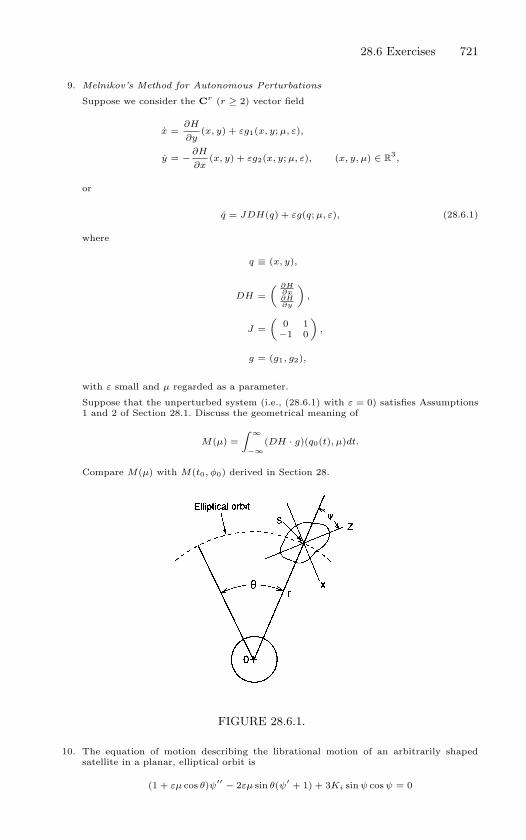
28.6 Exercises 721
9. Melnikov’s Method for Autonomous Perturbations
Suppose we consider the Cr (r ≥ 2) vector field
x =∂H
∂y(x, y) + εg1(x, y; µ, ε),
y = − ∂H
∂x(x, y) + εg2(x, y; µ, ε), (x, y, µ) ∈ R
3,
or
q = JDH(q) + εg(q; µ, ε), (28.6.1)
where
q ≡ (x, y),
DH =( ∂H
∂x∂H∂y
),
J =(
0 1−1 0
),
g = (g1, g2),
with ε small and µ regarded as a parameter.
Suppose that the unperturbed system (i.e., (28.6.1) with ε = 0) satisfies Assumptions1 and 2 of Section 28.1. Discuss the geometrical meaning of
M(µ) =∫ ∞
−∞(DH · g)(q0(t), µ)dt.
Compare M(µ) with M(t0, φ0) derived in Section 28.
FIGURE 28.6.1.
10. The equation of motion describing the librational motion of an arbitrarily shapedsatellite in a planar, elliptical orbit is
(1 + εµ cos θ)ψ′′ − 2εµ sin θ(ψ′ + 1) + 3Ki sin ψ cos ψ = 0
722 28. Melnikov’s Method
where ψ′ ≡ ∂ψ∂θ , Ki = Ixx−Izz
Iyy, ε is small, and εµ is the eccentricity of the orbit;
see Modi and Brereton [1969]. The geometry is illustrated in Figure 28.6.1. For εsmall, this equation can be written in the form (using the fact that 1
1+εµ cos θ =1 − εµ cos θ + O(ε2))
ψ′′ + 3Ki sin ψ cos ψ = ε[2µ sin θ(ψ′ + 1)
+ 3µKi sin ψ cos ψ cos θ] + O(ε2).
Use Melnikov’s method to study orbits homoclinic to hyperbolic periodic orbits forε = 0. Describe the physical manifestation of any chaotic dynamics that arise in thisproblem.
11. The driven Morse oscillator is an equation frequently used in theoretical chemistryto describe the photodissociation of molecules (see, e.g., Goggin and Milonni [1988]).The equation is given by
x = y,
y = −µ(
e−x − e
−2x)
+ εγ cos ωt,(28.6.2)
with µ, γ, ω > 0.
For ε = 0, the equation is Hamiltonian with Hamiltonian function
H(x, y) =y2
2+ µ
(−e
−x +12
e−2x
).
a) Show that for ε = 0, (x, y) = (∞, 0) is a nonhyperbolic fixed point of (28.6.2)that is connected to itself by a homoclinic orbit.
We would like to apply Melnikov’s theory to (28.6.2) in order to see if (28.6.2) hashorseshoes; however, the fixed point having the homoclinic orbit is nonhyperbolic.Therefore, the theory developed in this chapter does not immediately apply. Schecter[1987a], [1987b] has extended Melnikov’s method so that it applies to nonhyperbolicfixed points. However, we will not develop his technique.
Instead, we introduce the following transformation of variables
x = −2 log u, y = v, (28.6.3)
and reparametrize time as follows
ds
dt= − u
2.
b) Rewrite (28.6.2) in these new variables and show that the resulting equation,for ε = 0, has a hyperbolic fixed point at the origin that is connected to itselfby a homoclinic orbit. Apply Melnikov’s method in order to study homoclinicorbits for ε = 0.
c) Describe the resulting chaotic dynamics in both the x − y and u − v coordinatesystems.
This problem was originally solved by Bruhn [1989]. The transformation (28.6.3) isknown as a “McGehee transformation” in honor of Richard McGehee, who first cookedit up in order to study a degenerate fixed point at infinity in a celestial mechanics prob-lem (see McGehee [1974]). Such singularities frequently arise in mechanics and coordi-nate transformations such as (28.6.3) can greatly facilitate the analysis. An excellentintroduction to such problems can be found in Devaney [1982].
12. Consider the Cr (r ≥ 2) vector field
x = f1(x, y) + εg1(x, y, t; ε),
y = f2(x, y) + εg2(x, y, t; ε), (x, y) ∈ R2,
28.6 Exercises 723
orq = f(q) + εg(q, t; ε), (28.6.4)
where
q ≡ (x, y),
f ≡ (f1, f2),
g ≡ (g1, g2),
with ε small and g(q, t; ε) periodic in t with period T = 2π/ω.
Assumption: For ε = 0, (28.6.4) has a hyperbolic fixed point at p0 that is connectedto itself by a homoclinic orbit, q0(t), i.e., limt→±∞ q0(t) = p0.
a) Derive a measure of the distance between the stable and unstable manifolds ofthe hyperbolic periodic orbit that persists in (28.6.4) for ε sufficiently small.(Hint: follow the steps in this chapter as closely as possible. If you need help,see Melnikov [1963].)
b) Using the parametrization of the unperturbed homoclinic orbit in terms of(t0, φ0) ∈ R
1 × S1 as defined in (28.1.9), is the Melnikov function obtainedin part a) periodic in both t0 and φ0? Explain fully the reasons behind youranswer.
13. How is the Melnikov theory modified if in the unperturbed vector field we instead hadtwo hyperbolic fixed points, p1 and p2, connected by a heteroclinic orbit, q0(t), i.e.,limt→∞ q0(t) = p1 and limt→−∞ q0(t) = p2? (Hint: follow the development of thehomoclinic Melnikov theory in this chapter. You should arrive at the same formulafor the distance between the stable and unstable manifolds; however, the geometricalinterpretation will be different.)
14. Consider the vector field
θ = εv,
v = −ε sin θ + ε2γ cos ωt, (θ, v) ∈ S
1 × R1, ε small.
Apply Melnikov’s method to show that the Poincare map associated with this equationhas transverse homoclinic orbits. What problems arise? Can any conclusions be drawnfor homoclinic orbits arising in the following vector field?
θ = εv, (28.6.5)
v = −ε sin θ + ε2(−δv + γ cos ωt). (28.6.6)
What implications do these examples have for applying Melnikov’s method to vectorfields
x = εf(x, t), f − T -periodic in t, x ∈ R2,
that are transformed into
y = f(y) + εg(y, t), y ∈ R2, f(y) =
1T
∫ T
0f(y, t)dt,
by the method of averaging?
We refer the reader to Holmes, Marsden, and Scheurle [1988] and Delshams and Seara[1992] for more examples of problems of this type along with some rigorous results.
15. Consider the following vector field :
x = y,
y = x − x2 − εδy + εγ cos ωt.
Compute the Melnikov function and describe the surface in γ − δ − ω space where thebifurcation to homoclinic orbits occurs.
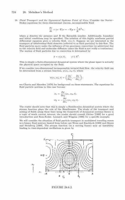
724 28. Melnikov’s Method
16. Fluid Transport and the Dynamical Systems Point of View. Consider the Navier–Stokes equations for three-dimensional viscous, incompressible fluid
∂v
∂t+ (v · ∇)v = −∇p +
1R
∇2v,
where p denotes the pressure and R the Reynolds number. Additionally, boundaryand initial conditions may be specified. The solution of this highly nonlinear partialdifferential equation gives a velocity field, v(x, t). Suppose we are interested in thetransport of infinitesimal fluid elements (referred to as fluid particles) in this flow. Thefluid particles move under the influence of two processes: convection (or advection) dueto the velocity field and molecular diffusion (since the fluid is not really a continuum).The motion of fluid particles due to convection is determined by
x = v(x, t), x ∈ R3.
This is simply a finite-dimensional dynamical system where the phase space is actuallythe physical space occupied by the fluid.
If we consider two-dimensional incompressible inviscid fluid flow, the velocity field canbe determined from a stream function, ψ(x1, x2; t), where
v(x1, x2, t) =(
∂ψ
∂x2, − ∂ψ
∂x1
);
see Chorin and Marsden [1979] for background on these statements. The equations forfluid particle motions in this case become
x1 =∂ψ
∂x2(x1, x2, t),
x2 = − ∂ψ
∂x1(x1, x2, t).
The reader should note that this is simply a Hamiltonian dynamical system where thestream function plays the role of the Hamiltonian. The study of the transport andmixing of fluids along these lines using the framework of dynamical systems theory isa topic of much current interest; the reader should consult Ottino [1989] for a goodintroduction and Rom-Kedar, Leonard, and Wiggins [1990] for a specific example.
We will consider the situation of fluid particle transport in modulated traveling wavesin a binary fluid mixture heated from below; see Weiss and Knobloch [1989] and Mosesand Steinberg [1988]. The stream function (in a moving frame) near an instabilityleading to time-dependent oscillations is given by
FIGURE 28.6.2.
28.6 Exercises 725
ψ(x1, x2, t) = ψ0(x1, x2) + εψ1(x1, x2, t),
whereψ0(x1, x2) = −x2 + R cos x1 sin x2,
ψ1(x1, x2, t) =γ
2
[(1 − 2
ω
)cos(x1 + ωt + θ)
+(
1 +2ω
)cos(x1 − ωt − θ)
]sin x2.
In the above ω > 0, θ is a phase, and R, γ, and ε are parameters (amplitude dependingon the temperature) with 0 < ε << 1; see Weiss and Knobloch [1989] for a detaileddiscussion. The equations for fluid particle motions are given by
x1 =∂ψ0
∂x2(x1, x2) + ε
∂ψ1
∂x2(x1, x2, t),
x2 = − ∂ψ0
∂x1(x1, x2) − ε
∂ψ1
∂x1(x1, x2, t).
For ε = 0, R > 1, the streamlines of the flow (corresponding to the level sets ofψ0(x1, x2)) appear as in Figure 28.6.2. Note the two hyperbolic fixed points on thex1-axis, denoted p+ and p−, respectively. The fixed points are connected by a pairof heteroclinic orbits denoted Γ0 and Γu. This heteroclinic cycle forms a region oftrapped fluid that is shaded in Figure 28.6.2.
a) For ε = 0 show that Γ0 persists and results in a barrier which fluid cannot cross.
b) Show that for ε = 0, Γu breaks up giving rise to transverse heteroclinic orbits.This provides a mechanism for fluid to mix between the two regions in the time-dependent fluid flow.
c) Show that a horseshoe exists in the heteroclinic tangle for ε = 0. (Hint: seeRom-Kedar et al. [1990].) Hence, chaotic fluid particle trajectories exist.
29
Liapunov Exponents
A positive Liapunov exponent is often taken as a signature of chaos. Wewill address this specific question in Chapter 30. But in this chapter wediscuss Liapunov exponents following Oseledec [1968] and Benettin et al.
[1980a, b].
29.1 Liapunov Exponents of a Trajectory
Consider the Cr (r ≥ 1) vector field
x = f(x), x ∈ Rn. (29.1.1)
Let x(t, x0) be a trajectory of (29.1.1) satisfying x(0, x0) = x0. We want todescribe the orbit structure of (29.1.1) near x(t, x0). In particular, we wantto know the geometry associated with the attraction and/or repulsion oforbits of (29.1.1) relative to x(t, x0). For this it is natural to first considerthe orbit structure of the linearization of (29.1.1) about x(t, x0) given by
ξ = Df(x(t))ξ, ξ ∈ Rn. (29.1.2)
Let X(t;x(t, x0)) be the fundamental solution matrix of (29.1.2) and lete = 0 be a vector in R
n. Then the coefficient of expansion in the direction
e along the trajectory through x0 is defined to be
λt(x0, e) ≡‖X(t;x(t, x0))e‖
‖e‖ , (29.1.3)
where ‖ · ‖ =√〈·, ·〉 with 〈·, ·〉 denoting the standard scalar product on
Rn. Note that λt(x0, e) is a time-dependent quantity that also depends
on a particular orbit of (29.1.1) (through the fundamental solution matrixX(t;x(t, x0))), a particular point along this orbit, and a particular directionalong this orbit. The Liapunov characteristic exponent (or just Liapunov
29.1 Liapunov Exponents of a Trajectory 727
exponent) in the direction e along the trajectory through x0 is defined tobe
χ(X(t;x(t, x0)), x0, e) ≡ limt→∞
1t
log λt(x0, e). (29.1.4)
We make several remarks concerning this definition.
1. Equation (29.1.4) is an asymptotic quantity. Therefore, in order forit to make sense, we must at least know that x(t, x0) exists for allt > 0. This will be true if the phase space is a compact, boundarylessmanifold or if x0 lies in a positively invariant region.
2. For the zero vector we define χ(X(t;x(t, x0)), x0, 0) = −∞.
3. The fundamental solution matrix, X(t;x(t, x0)), of (29.1.2) is asso-ciated with a particular trajectory, x(t, x0), of (29.1.1). Thus, if weconsidered a different trajectory, x(t, x0), of (29.1.1), then the fun-damental solution matrix associated with the vector field linearizedabout x(t, x0) may (and most probably will) have different properties.
4. The Liapunov exponent in the direction e along the orbit throughx0 is unchanged if the initial condition of the trajectory along theorbit is varied. In particular, for any t1 ∈ R, let x(t1, x0) ≡ x1;then χ(X(t;x(t, x0)), x0, e) = χ(X(t;x(t, x0)), x1, e). This should beintuitively clear from the fact that the exponents are limits as t →∞;see Exercise 1.
5. In light of the previous remark it makes sense to drop the initial con-dition of the trajectory from the notation for a Liapunov exponent,i.e., χ(X(t; x(t, x0)), x0, e) = χ(X(t;x(t, x0)), e). Moreover, our dis-cussions in this subsection will be concerned with Liapunov exponentsassociated with a given trajectory, and, hence, a given fundamentalsolution matrix X(t;x(t, x0)). In this setting we will further simplifythe notation by dropping the explicit dependence on the fundamentalsolution matrix X(t;x(t, x0)), i.e., χ(X(t; x(t, x0)), e) = χ(e).
6. In general, Liapunov exponents are not continuous functions of theorbits. This can be seen from Example 29.2.3.
Next we want to develop some geometrical properties of the Liapunovexponents associated with a given trajectory. The following lemma is fun-damental in this regard.
Lemma 29.1.1 For any vectors f, g ∈ Rn, and nonzero constant c ∈ R,
728 29. Liapunov Exponents
χ(f + g) ≤ max χ(f), χ(g) , (29.1.5)
χ(cg) = χ(g). (29.1.6)
Proof: This follows immediately from the definition of Liapunov exponentsgiven in (29.1.4).
This lemma, along with the standard definition of a vector space, impliesthe following proposition.
Proposition 29.1.2 For any r ∈ R
g ∈ Rn |χ(g) ≤ r
is a vector subspace of Rn.
From this proposition we can conclude that there are at most n (i.e., thedimension of the phase space) distinct Liapunov exponents associated witha trajectory. More precisely, we have the following result.
Proposition 29.1.3 The set of numbers
χ(g)g∈Rn
g =0,
takes at most n = dim Rn values, which we denote by
ν1 > · · · > νs, 1 ≤ s ≤ n.
Proof: See Exercise 2.
Associated with the s distinct values for the Liapunov exponents we haves + 1 nested subspaces.
Proposition 29.1.4 Let Li = g ∈ Rn |χ(g) ≤ νi. Then
0 ≡ Ls+1 ⊂ Ls ⊂ · · · ⊂ L1 = Rn
with Li+1 = Li and χ(g) = νi if and only if g ∈ Li\Li+1, 1 ≤ i ≤ s.
29.1 Liapunov Exponents of a Trajectory 729
Proof: This is an immediate consequence of Proposition 29.1.2 and Propo-sition 29.1.3.
Next we define the notion of the spectrum of Liapunov exponents asso-ciated with X(t;x(t, x0)).
Definition 29.1.5 (Spectrum of X(t;x(t, x0))) The numbers ν1, · · · , νs
are referred to as the spectrum of Liapunov exponents associated withX(t;x(t, x0)), and denoted by sp (X(t;x(t, x0))). The multiplicity of νi is
denoted by ki, and is given by ki ≡ dimLi − dimLi+1, 1 ≤ i ≤ s.
Next we want to consider conditions under which the limit, rather thanthe lim sup, in (29.1.4) exists. First we need two definitions.
Definition 29.1.6 (Normal Basis) A basis e1, · · · , en of Rn is said to
be a normal basis ifn∑
i=1
χ(ei) ≤n∑
i=1
χ(fi),
where f1, · · · , fn is any other basis of Rn.
Definition 29.1.7 (Regular Family) The fundamental solution matrix
X(t;x(t, x0)) is called regular as t →∞ if
1. limt→∞1t log |det X(t; x(t, x0))| exists and is finite, and
2. for each normal basis e1, · · · , enn∑
i=1
χ(ei) = limt→∞
1t
log |det X(t;x(t, x0))|.
Now we can state the main existence theorem due to Liapunov [1966].
Theorem 29.1.8 If X(t;x(t, x0)) is regular as t →∞, then
χ(e) = limt→∞
1t
log λt(x0, e) (29.1.7)
exists and is finite for any vector e ∈ Rn.
730 29. Liapunov Exponents
Proof: See Liapunov [1966], Oseledec [1968], or Benettin et al. [1980a].
This immediately raises the question of whether or not a particularfundamental solution matrix is regular. This problem was addressed byOseledec [1968] and is answered (in a sense) in the Oseledec multiplica-
tive ergodic theorem. Oseledec showed that, with respect to some invariantmeasure, almost all trajectories give rise to regular fundamental solutionmatrices. There are a number of technical issues associated with statingthis fundamental theorem, and we refer the reader to Oseledec [1968] andBenettin et al. [1980a] for more details.
Liapunov exponents are just one type of spectra one can associate witha linear, time-varying system. There are others (e.g., we introduced thenotion of exponential dichotomy in Chapter 3). A survey of different spectrafor linear systems is given in Dieci and van Vleck [2002].
Some new insights into the behavior of Liapunov exponents, and theirgeneralizations, have been obtained by Colonius and Kliemann by combin-ing methods of nonlinear geometric control theory with dynamical systemstheory. See Colonius and Kliemann [1996b], and references therein.
29.2 Examples
Let us now consider a few examples.
Example 29.2.1 (A Linear, Homogeneous, Constant Coefficient System). Con-
sider the linear, scalar vector field
x = ax, x ∈ R1, (29.2.1)
where a is a constant. Equation (29.2.1) has three orbits, x = 0, x > 0, and
x < 0, but the fundamental solution matrix associated with each orbit is given
by
X(t) = eat. (29.2.2)
Thus, using (29.2.2) and (29.1.7), we see that each orbit of (29.2.1) has only one
Liapunov exponent, and the Liapunov exponent of each orbit is a. Thus, if a > 0,
trajectories of (29.2.1) separate exponentially as t → ∞.
End of Example 29.2.1
Example 29.2.2 (An Integrable System). Consider a planar, Hamiltonian sys-
tem in a region of phase space where the vector field is given in action-angle
29.2 Examples 731
variables as followsI = 0,θ = Ω(I),
(I, θ) ∈ R+ × S1. (29.2.3)
Then, a trajectory of (29.2.3) is given by
I = constant,θ(t) = Ω(I)t + θ0.
(29.2.4)
Linearizing (29.2.3) about (29.2.4) gives(ξ1
ξ2
)=
(0 0
∂Ω∂I
(I) 0
)(ξ1
ξ2
). (29.2.5)
The fundamental solution matrix of (29.2.5) is easily computed and found to be
X(t) =
(C C
C ∂Ω∂I
(I)t 0
), (29.2.6)
where C is a constant. Letting δθ represent a vector tangent to a trajectory and
δI a vector normal to a trajectory using (29.2.6) and (29.1.7), we easily obtain
χ(I, δI) = 0,
χ(I, δθ) = 0,
for any I labeling a trajectory of (29.2.3) defined by (29.2.4).
End of Example 29.2.2
Example 29.2.3 (A Two-Dimensional, Autonomous, Nonlinear System). Con-
sider the vector field
x = x − x3,
y = −y. (29.2.7)
In Example 8.2.2 of Chapter 8, we saw that (29.2.7) has a saddle at (x, y) = (0, 0)
and sinks at (±1, 0). Moreover, the closed interval [−1, 1] on the x-axis is an
attracting set; see Figure 29.2.1.
We want to compute the Liapunov exponents associated with orbits in this
attracting set. The attracting set [−1, 1] contains five orbits, the fixed points
(x, y) = (0, 0), (±1, 0) and the open intervals (−1, 0) and (0, 1). Each orbit has
two Liapunov exponents. We will compute the Liapunov exponents of each orbit
individually. We let δx ≡ (1, 0) denote a tangent vector in the x direction and
δy ≡ (0, 1) denote a tangent vector in the y direction. It should be clear that
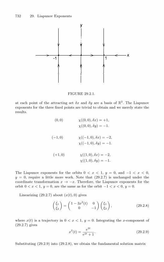
732 29. Liapunov Exponents
FIGURE 29.2.1.
at each point of the attracting set δx and δy are a basis of R2. The Liapunov
exponents for the three fixed points are trivial to obtain and we merely state the
results.
(0, 0) χ((0, 0), δx) = +1,
χ((0, 0), δy) = −1.
(−1, 0) χ((−1, 0), δx) = −2,
χ((−1, 0), δy) = −1.
(+1, 0) χ((1, 0), δx) = −2,
χ((1, 0), δy) = −1.
The Liapunov exponents for the orbits 0 < x < 1, y = 0, and −1 < x < 0,
y = 0, require a little more work. Note that (29.2.7) is unchanged under the
coordinate transformation x → −x. Therefore, the Liapunov exponents for the
orbit 0 < x < 1, y = 0, are the same as for the orbit −1 < x < 0, y = 0.
Linearizing (29.2.7) about (x(t), 0) gives(ξ1
ξ2
)=
(1 − 3x2(t) 0
0 −1
)(ξ1
ξ2
), (29.2.8)
where x(t) is a trajectory in 0 < x < 1, y = 0. Integrating the x-component of
(29.2.7) gives
x2(t) =
e2t
e2t + 1. (29.2.9)
Substituting (29.2.9) into (29.2.8), we obtain the fundamental solution matrix
29.2 Examples 733
X(t) =
(e−2t(1 + e−2t)−3/2 0
0 e−t
). (29.2.10)
Using (29.1.7) and (29.2.10), we obtain the Liapunov exponents
0 < x < 1, y = 0 χ((0 < x < 1, y = 0), δx) = −2,
χ((0 < x < 1, y = 0), δy) = −1,
−1 < x < 0, y = 0 χ((−1 < x < 0, y = 0), δx) = −2,
χ((−1 < x < 0, y = 0), δy) = −1.
End of Example 29.2.3
We end this section with some final remarks.
Remark 1. We can view the Liapunov exponents of a given orbit as thelong time average of the real parts of the eigenvalues of the fundamentalsolution matrix associated with the linearization of the vector field aboutthe orbit. Therefore, they give us information concerning local expansionand contraction of phase space only and nothing about twisting and folding.
Remark 2. It should be clear that if the orbit is a fixed point or periodicorbit, then the Liapunov exponents are, in the first case, the real partsof the eigenvalues associated with the matrix of the vector field linearizedabout the fixed point and, in the second case, the real parts of the Floquetexponents. Thus, in some sense the theory of Liapunov exponents is ageneralization of linear stability theory for arbitrary trajectories (but seeGoldhirsch et al. [1987]).
This brings up an interesting point. Associated with the lineareigenspaces associated with vector fields linearized about fixed points andperiodic orbits are manifolds invariant under the full nonlinear dynamicswhere orbits have the same asymptotic behavior as in the linearized system.We refer to these as the stable and unstable manifolds. Might an arbitrary
orbit possess stable and unstable manifolds having dimension equal to thenumber of negative and positive Liapunov exponents, respectively, associ-ated with the orbit? The answer to this question is yes, and it has beenproved by Pesin [1976], [1977], but see also Sacker and Sell [1974], [1976a],[1976b], [1978], and [1980].
We have only hinted in this section at the various properties of Lia-punov exponents. For more information the reader should consult Liapunov
734 29. Liapunov Exponents
[1966], Bylov et al. [1966], Oseledec [1968], Ledrappier and Young [1991],and Young [1982]. We develop many additional properties of Liapunov ex-ponents in the exercises.
29.3 Numerical Computation of LiapunovExponents
In applications the Liapunov exponents of a trajectory will need to becomputed numerically. There has been much rigorous work in recent yearsinvolving the accurate computation of Liapunov exponents. Two papersthat discuss this problem with great detail and rigour are Dieci et al. [1997]and Bridges and Reich [2001]. The paper of Dieci et al. [1997] is notablefor providing error estimates for the finite time computations1. Dieci [2002]describes algorithms for computing Liapunov exponents that do not requirethe computation of a Jacobian. Related work can be found in Rangarajanet al. [1998] and Janaki et al. [1999]. These numerical approaches involveeither a QR or a singular value decomposition (SVD) of the fundamentalsolution matrix. While the theory of QR and SVD for constant matricesis well-known, the fundamental solution matrix varies in time. The theoryfor QR and SVD of time varying matrices is developed in Dieci and Eirola[1999] amd Dieci and van Vleck [1999]. Methods for computing Liapunovexponents that are specific to Hamiltonian systems can be found in Partovi[1999] and Yamaguchi and Iwai [2001]. The paper of Ramasubramanian andSriram [2000] provides a comparative study between different algorithmsfor the computation of Liapunov exponents. The work of Udwadia and vonBremen [2001], [2002] is also notable.
29.4 Exercises
1. Recall the discussion earlier in this chapter. Show that
χ(x0, e) = χ(x(T ), e)
for any finite T .
2. Prove Proposition 29.1.3.
3. Consider a planar, Hamiltonian vector field. Must all Liapunov exponents of everyorbit be zero?
1Liapunov exponents are asymptotic quantities. They are defined in the limitas time approaches infinity. Obviously, this limit cannot be realized on a com-puter, and therefore some error is incurred.
29.4 Exercises 735
4. Show that any trajectory of a vector field that remains bounded and does not terminateon a fixed point must have at least one zero Liapunov exponent. (Hint: consider thedirection tangent to the orbit.)
5. In any realistic example, the Liapunov exponents of an orbit must be calculated nu-merically. In this case, you can see that a problem may arise. Namely, a Liapunovexponent is a number obtained in the limit t → ∞, and, in practice, one can onlycompute for a finite amount of time.
Recall Example 29.2.3. Consider an initial condition
(x, y) = (ε, 0),
and the directionδx = (1, 0).
Letχt(x0, e) =
1t
log λt(x0, e),
and computeχt((ε, 0), δx)
for this example. It should follow from the discussion in the example that for some Twe have
χt((ε, 0), δx) ≤ 0, t ∈ [T, ∞).
Let T0(ε) be the value of t such that
χT0(ε)((ε, 0), δx) = 0.
a) Compute T0(ε) and graph it as a function of ε.
b) What can you conclude from this example concerning the numerical computationof Liapunov exponents?
6. Consider a linear velocity field given by:
(x1x2
)=
(cos 4t sin 4t − 2
sin 4t + 2 − cos 4t
)(x1x2
). (29.4.1)
Verify that the solution of (29.4.1) is given by:
x1(t) = x10et cos 2t − x20e
−t sin 2t,
x2(t) = x10et sin 2t + x20e
−t cos 2t. (29.4.2)
(a) What is the fundamental solution matrix associated with (29.4.1)?
(b) Compute the Liapunov exponents associated with this fundamental solutionmatrix.
30
Chaos and Strange Attractors
In this chapter we want to examine what is meant by the term “chaos”as applied to deterministic dynamical systems as well as the notion of a“strange attractor.” We will begin by giving several definitions of propertiesthat should be characteristic of “chaos” and then consider several examplesthat possess one, several, or all of these properties.
We consider Cr (r ≥ 1) autonomous vector fields and maps on Rn de-
noted as follows
vector field x = f(x), (30.0.1)map x → g(x). (30.0.2)
We denote the flow generated by (30.0.1) by φ(t, x) and we assume thatit exists for all t > 0. We assume that Λ ⊂ R
n is a compact set invariantunder φ(t, x) (resp. g(x)), i.e., φ(t,Λ) ⊂ Λ for all t ∈ R (resp. gn(Λ) ⊂ Λfor all n ∈ Z, except that if g is not invertible, we must take n ≥ 0). Thenwe have the following definitions.
Definition 30.0.1 (Sensitive Dependence on Initial Conditions)The flow φ(t, x) (resp. g(x)) is said to have sensitive dependence on initialconditions on Λ if there exists ε > 0 such that, for any x ∈ Λ and any
neighborhood U of x, there exists y ∈ U and t > 0 (resp. n > 0) such that
|φ(t, x)− φ(t, y)| > ε (resp. |gn(x)− gn(y)| > ε).
Roughly speaking, Definition 30.0.1 says that for any point x ∈ Λ, thereis (at least) one point arbitrarily close to Λ that diverges from x. Someauthors require the rate of divergence to be exponential; for reasons to beexplained later, we will not do so. As we will see in the examples, taken byitself sensitive dependence on initial conditions is a fairly common featurein many dynamical systems.
Definition 30.0.2 (Chaotic Invariant Set) Λ is said to be chaotic if
30. Chaos and Strange Attractors 737
1. φ(t, x) (resp. g(x)) has sensitive dependence on initial conditions on
Λ.
2. φ(t, x) (resp. g(x)) is topologically transitive on Λ.
Some authors (e.g., Devaney [1986]) add an additional requirement toDefinition 30.0.2. For further discussions of the definition of chaos see Glas-ner and Weiss [1993] and Banks et al. [1992].
3. The periodic orbits of φ(t, x) (resp. g(x)) are dense in Λ.
We will not explicitly include point 3 as part of the definition of achaotic invariant set, but we will examine its importance and relationshipto “chaos.”
We will now consider several examples that exhibit the properties de-scribed in these two definitions.
Example 30.0.1. Consider the following vector field on R1
x = ax, x ∈ R1, (30.0.3)
with a > 0. The flow generated by (30.0.3) is given by
φ(t, x) = eatx. (30.0.4)
From (30.0.4) we conclude the following.
1. φ(t, x) has no periodic orbits.
2. φ(t, x) is topologically transitive on the noncompact sets (0, ∞) and
(−∞, 0).
3. φ(t, x) has sensitive dependence on initial conditions on R1 since for any
x0, x1 ∈ R1, with x0 = x1,
|φ(t, x0) − φ(t, x1)| = eat|x0 − x1|.
Hence, the distance between any two points grows (exponentially) in time.
End of Example 30.0.1
738 30. Chaos and Strange Attractors
Example 30.0.2. Consider the vector field
r = sinπ
r,
θ = r, (r, θ) ∈ R+ × S1. (30.0.5)
The flow generated by (30.0.5) has a countable infinity of periodic orbits given
by
(r(t), θ(t)) =
(1
n,
t
n+ θ0
), n = 1, 2, 3, · · · . (30.0.6)
It is easy to verify that the periodic orbits are stable for n even and unstable for
n odd. Hence, in a compact region of the phase space, (30.0.5) has a countable
infinity of unstable periodic orbits. We leave it as an exercise for the reader
to verify that (30.0.5) may exhibit sensitive dependence on initial conditions
in (open) annuli bounded by adjacent stable periodic orbits (see Exercise 2).
However, (30.0.5) is only topologically transitive in the (open) annuli bounded
by adjacent stable and unstable periodic orbits.
End of Example 30.0.2
Example 30.0.3. Consider the vector field on the two torus, T 2 ≡ S1 × S1
θ1 = ω1,
θ2 = ω2, (θ1, θ2) ∈ T 2, (30.0.7)
withω1
ω2= irrational. (30.0.8)
Then, it follows from Chapter 10, Section 10.4a, that the flow generated by
(30.0.7) is topologically transitive on T 2. From (30.0.8) it is easy to see that
the flow generated by (30.0.7) has no periodic orbits. We leave it as an exercise
for the reader (see Exercise 3) to show that on T 2 the flow generated by (30.0.7)
does not have sensitive dependence on initial conditions.
End of Example 30.0.3
Example 30.0.4. Consider the following integrable twist map(Iθ
)→
(I
2πΩ(I) + θ
)≡
(f1(I, θ)f2(I, θ)
), (I, θ) ∈ R
+ × S1, (30.0.9)
and∂Ω
∂I(I) = 0 (twist condition). (30.0.10)
30. Chaos and Strange Attractors 739
The nth iterate of (30.0.9) is easily calculated and is given by(Iθ
)→
(I
2πnΩ(I) + θ
)≡
(fn1 (I, θ)
fn2 (I, θ)
). (30.0.11)
The simple form of (30.0.9) and (30.0.11) enable us to easily verify the following.
1. Equation (30.0.9) is not topologically transitive, since all orbits remain on
invariant circles.
2. The periodic orbits of (30.0.9) are dense in the phase space. This uses the
twist condition.
3. Equation (30.0.9) has sensitive dependence on initial conditions due to the
twist condition. This can be seen as follows. For (I0, θ0), (I1, θ1) ∈ R+×S1,
with I0 = I1, we have
|(fn1 (I0, θ0) − fn
1 (I1, θ1)), (fn2 (I0, θ0) − fn
2 (I1, θ1))|= |((I0 − I1), (2πn(Ω(I0) − Ω(I1)) + (θ0 − θ1))|. (30.0.12)
Therefore, from (30.0.10), Ω(I0)− Ω(I1) = 0. Thus, we see from (30.0.12) that
as n increases, the θ components of nearby points drift apart. However, the rate
of separation is not exponential.
End of Example 30.0.4
Example 30.0.5. Consider
σ: ΣN −→ Σ
N , (30.0.13)
where ΣN is the space of bi-infinite sequences of N symbols and σ is the shift
map as described in Chapter 24. Then we have proven the following.
1. ΣN is compact and invariant (see Proposition 24.1.4).
2. σ is topologically transitive, i.e., σ has an orbit that is dense in ΣN (see
Proposition 24.2.2).
3. σ has sensitive dependence on initial conditions (see Section 23.5).
4. σ has a countable infinity of periodic orbits (see Proposition 24.2.2) that
are dense in ΣN (see Exercise 4).
Thus, ΣN is a chaotic, compact invariant set for σ. From Chapters 25, 26,
and 27 we know that two-dimensional maps and three-dimensional autonomous
vector fields may possess compact invariant sets on which the dynamics are topo-
logically conjugate to (30.0.13). In all of these cases, homoclinic (and possibly
740 30. Chaos and Strange Attractors
heteroclinic) orbits are the underlying mechanism that gives rise to such behav-
ior. This is important, because this knowledge enables us to develop techniques
(e.g., Melnikov’s method) that predict (in terms of the system parameters) when
chaotic dynamics occur in specific dynamical systems.
End of Example 30.0.5
We make the following remarks concerning these examples.
Remark 1. Example 30.0.1 illustrates why we require chaotic invariant setsto be compact.
Remark 2. Example 30.0.2 illustrates why having an infinite number ofunstable periodic orbits in a compact, invariant region of phase space isnot by itself a sufficient condition for chaotic dynamics.
Remark 3. Example 30.0.3 describes a vector field having a compact invari-ant set (which is actually, the entire phase space) on which the dynamicsare topologically transitive, but it does not have sensitive dependence oninitial conditions.
Remark 4. Example 30.0.4 describes a two-dimensional integrable map thathas sensitive dependence on initial conditions and the periodic orbits aredense in the phase space, but it is not topologically transitive.
Thus, taken together, Examples 30.0.1 through 30.0.4 show the impor-tance of Definition 30.0.2 being satisfied completely. Example 30.0.5 showshow chaotic dynamics can arise in many dynamical systems. However, itdoes not address the question of observability.
Definition 30.0.3 (Strange Attractor) Suppose A ⊂ Rn is an attrac-
tor. Then A is called a strange attractor if it is chaotic.
Hence, if we want to prove that a dynamical system has a strange at-tractor we might proceed as follows.
Step 1. Find a trapping region, M, in the phase space (see Definition 8.2.2in Chapter 8).
Step 2. Show that M contains a chaotic invariant set Λ. In practice, thismeans showing that inside M is a homoclinic orbit (or heteroclinic
30. Chaos and Strange Attractors 741
cycle) which has associated with it an invariant Cantor set on whichthe dynamics are topologically conjugate to a full shift on N symbols(recall Chapters 26 and 27).
Step 3. Then, from Definition 8.2.1 in Chapter 8,
⋂t>0
φ(t,M)
(resp.
⋂n>0
gn(M)
)≡ A (30.0.14)
is an attracting set. Moreover, Λ ⊂ A (see Exercise 5) so that Acontains a mechanism that gives rise to sensitive dependence on initialconditions; in order to conclude that A is a strange attractor we needonly demonstrate the following.
1. The sensitive dependence on initial conditions on Λ extends toA;
2. A is topologically transitive.
Hence, in just three steps we can show that a dynamical system possessesa strange attractor. In this book we have developed techniques and seenexamples of how to carry out Steps 1 and 2. However, the third step is thekiller, namely, showing that A is topologically transitive. This is because asingle, stable orbit in A will destroy topological transitivity and, in Chap-ter 32, we will see that periodic sinks are always associated with quadratichomoclinic tangencies. Moreover, as a result of Newhouse’s work, at leastfor two-dimensional dissipative maps, these homoclinic tangencies are per-sistent in the sense that if we destroy a particular tangency we will createanother elsewhere in the homoclinic tangle. This is largely the reason whythere is yet to be an analytical proof of the existence of a strange attractorfor the periodically forced, damped Duffing oscillator, despite an enormousamount of numerical evidence. However, Wang and Young [2002] give aresult that proves the existence of a strange attractor for “sufficently largedamping”.
At present, there exist rigorous results concerning strange attractors (byour Definition 30.0.3) in the following areas.
1. One-Dimensional Non-Invertible Maps. For maps such as
x → µx(1− x)
orx → x2 − µ
742 30. Chaos and Strange Attractors
with µ a parameter there now exists a fairly complete existence theoryfor strange attractors. The reader should consult Jakobsen [1981], Mi-siurewicz [1981], Johnson [1987], Guckenheimer and Johnson [1990],and de Melo and van Strien [1993].
2. Hyperbolic Attractors of Two-Dimensional Maps. Plykin [1974], Ne-mytskii and Stepanov [1989] and Newhouse [1980] have constructedexamples of hyperbolic attracting sets which satisfy Definition 30.0.2.These examples are somewhat artificial in the sense that one wouldnot expect them to arise in Poincare maps of ordinary differentialequations that arise in typical applications.
3. Lorenz-Like Systems. The topology associated with the Lorenz equa-tions (see Sparrow [1982]) avoids many of the problems associatedwith Newhouse sinks. Consequently, in the past few years there hasbeen much progress in proving that the Lorenz equations (along withslightly modified versions of the Lorenz equations) possess a strangeattractor. The reader is referred to Sinai and Vul [1981], Afraimovich,Bykov, and Silnikov [1983], Rychlik [1990], and Robinson [1989]. Re-cently, an elegant computer assisted proof of the existence of a strangeattractor for the Lorenz equations was given by Tucker [1999]; see alsoMorales et al. [1998] and the popular articles of Stewart [2000] andViana [2000].
4. The Henon Map. The Henon map is defined to be
x → y,y → −εx + µ− y2, (30.0.15)
where ε and µ are parameters. Over the past ten years a large amountof numerical evidence has suggested the existence of a strange attrac-tor in this map. Recently, Benedicks and Carleson [1991] have proventhat, for ε small, (30.0.15) does indeed possess a strange attractor.
5. Recent Results on Strange Attractors. For recent work on strangeattractors see Palis and Takens [1993], Mora and Viana [1993], Diazet al. [1996], Naudot [1996], and Turaev and Silnikov [1998].
6. Strange Attractors for Nonautonomous Vector Fields. If the nonau-tonomous vector field is time-periodic, then its study can be reducedto an associated Poincare map (Chapter 10) and strange attractorresults for maps can be applied. A very thorough discussion of thiscan be found in Wang and Young [2002].
If the vector field is not time-periodic, then many new issues arise.The notion of an attractor for general nonautonomous systems wasdescribed in Chapter 8, Section 8.4. In addition to the notion of at-tractors for such vector fields, a definition and characterization of
30. Chaos and Strange Attractors 743
chaos must be given. This has been considered in Scheurle [1986],Wiggins [1988], [1999], Stoffer [1988a,b], Meyer and Sell [1989], andLerman and Silnikov [1992]. With notions of “attraction” and “chaos”in hand for nonautonomous vector fields with arbitrary time depen-dence one should be able to develop a notion of “strange attractor”.Nevertheless, this is a subject which has not been developed, bothfrom the point of view of rigorous mathematical results, and specificexamples.
Thus, the “strange attractor problem” is still far from being solved ingeneral. In particular, there is a need for thoroughly studied examples inhigher dimensions, for vector fields in dimensions larger than three andfor maps of dimension larger than two. A variety of examples of systemsundergoing (rigorously proven) chaotic behavior in high dimensions can befound; however, the attractive nature of the chaos in these examples hasnot been studied.
If a dynamical system possesses a chaotic invariant set, then an obviousquestion arises: namely, how is the chaos manifested in terms of “random”or “unpredictable” behavior of the system? The answer to this questiondepends on the geometry of the construction of the chaotic invariant setand, thus, the answer varies from problem to problem (as we should expect).Let us consider an example, our old friend the periodically forced, dampedDuffing oscillator.
This system is given by
x = y,y = x− x3 + ε(−δy + γ cos ωt). (30.0.16)
We know from Chapter 28 that, for ε sufficiently small and δ <(3πω sech(πω/2)2√
2
)γ, the Poincare map associated with (30.0.16) possesses
transverse homoclinic orbits to a hyperbolic fixed point. Theorem 26.0.5implies that (30.0.16) has chaotic dynamics. However, we want to interpretthis chaos specifically in terms of the dynamics of (30.0.16). We will dothis by constructing the chaotic invariant set geometrically and describ-ing the associated symbolic dynamics geometrically. Our discussion will beheuristic, but, at this stage, the reader should easily be able to supply thenecessary rigor (see Exercise 7).
Consider the two “horizontal” strips labeled H+ and H− in Figure 30.0.1.
Under the Poincare map, denoted P , H+ and H− are mapped over them-selves in iterates as shown heuristically in Figure 30.0.1. It should be clearthat the horizontal (resp. vertical) boundaries of H+ and H− map to hor-
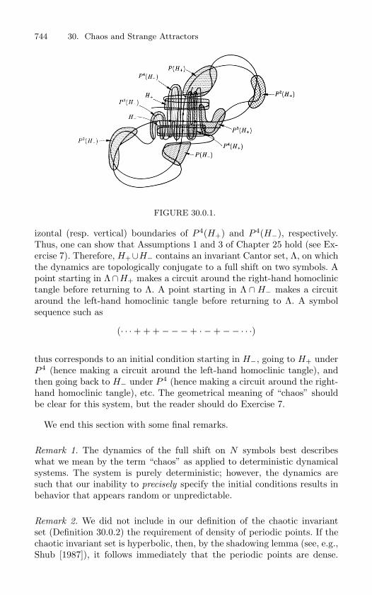
744 30. Chaos and Strange Attractors
FIGURE 30.0.1.
izontal (resp. vertical) boundaries of P 4(H+) and P 4(H−), respectively.Thus, one can show that Assumptions 1 and 3 of Chapter 25 hold (see Ex-ercise 7). Therefore, H+∪H− contains an invariant Cantor set, Λ, on whichthe dynamics are topologically conjugate to a full shift on two symbols. Apoint starting in Λ∩H+ makes a circuit around the right-hand homoclinictangle before returning to Λ. A point starting in Λ ∩ H− makes a circuitaround the left-hand homoclinic tangle before returning to Λ. A symbolsequence such as
(· · ·+ + +−−−+ · −+−− · · ·)
thus corresponds to an initial condition starting in H−, going to H+ underP 4 (hence making a circuit around the left-hand homoclinic tangle), andthen going back to H− under P 4 (hence making a circuit around the right-hand homoclinic tangle), etc. The geometrical meaning of “chaos” shouldbe clear for this system, but the reader should do Exercise 7.
We end this section with some final remarks.
Remark 1. The dynamics of the full shift on N symbols best describeswhat we mean by the term “chaos” as applied to deterministic dynamicalsystems. The system is purely deterministic; however, the dynamics aresuch that our inability to precisely specify the initial conditions results inbehavior that appears random or unpredictable.
Remark 2. We did not include in our definition of the chaotic invariantset (Definition 30.0.2) the requirement of density of periodic points. If thechaotic invariant set is hyperbolic, then, by the shadowing lemma (see, e.g.,Shub [1987]), it follows immediately that the periodic points are dense.
30.1 Exercises 745
Moreover, Grebogi et al. [1985] have obtained numerical evidence for theexistence of chaotic attractors in maps of the N -torus which have the prop-erty that orbits in the attractor densely cover the N -torus.
Remark 3. In our definition of sensitive dependence on initial conditions(Definition 30.0.1) we did not require the separation rate to be exponential.This is because it appears now that the strange attractors observed innumerical experiments of typical dynamical systems arising in applicationswill not, in general, be hyperbolic. Hence, one should expect parts of theattractor to exhibit nonexponential contraction or expansion rates. This isan area where new analytical techniques need to be developed.
Remark 4. Positive Liapunov exponents have been a standard criterion fordeciding when a dynamical system is “chaotic” over the past few years.Examples 29.2.1 and 29.2.3 show that this criterion should be interpretedwith caution; see also Exercise 5 following Chapter 29.
Remark 5. In an interesting series of papers, Brown and Chua [1996a,b],[1998] describe relationships between different characterizations of chaos ingreat detail.
30.1 Exercises
1. Can a Cr map or flow depend on initial conditions in a Cr manner and also exhibitsensitive dependence on initial conditions? Explain.
2. Recall Example 30.0.2. Do all or only some orbits in the open annuli bounded byadjacent stable periodic orbits exhibit sensitive dependence on initial conditions?
3. Recall Example 30.0.3. Show that the flow generated by (30.0.7) is topologically tran-sitive on T 2.
4. Show that for the dynamical system
σ: ΣN → ΣN
the periodic orbits are dense in ΣN .
5. Letx → g(x), x ∈ R
n,
be a Cr (r ≥ 1) map. Suppose M ⊂ Rn is a trapping region with Λ ⊂ M a chaotic
invariant set. Then definingA ≡
⋂n>0
gn(M),
show thatΛ ⊂ A.
6. Very often one hears the phrase,
746 30. Chaos and Strange Attractors
A dynamical system is chaotic if it has one positive Liapunov exponent.
Discuss what this phrase means in light of the discussion in Sections 29 and 30. Con-sider both dissipative and nondissipative systems.
7. Recall the discussion of chaos in the phase space of the damped, periodically forcedDuffing oscillator at the end of Section 30. The goal of this exercise is to make theheuristic arguments given in that discussion rigorous.
a) Draw the homoclinic tangle correctly for the Poincare map on a given cross-section (say Σ0). You may want to use a computer.
b) Find candidates for two µh-horizontal strips, denoted H0 and H1, which mapover themselves in µv-vertical strips under some iterate of the Poincare mapso that Assumptions 1 and 3 of Chapter 25 are satisfied. Choose the horizon-tal strips so that the relationship between the motion in phase space and thedynamics on the invariant set is as described in Chapter 30.
c) Describe the relationship between the number of iterates needed to form thechaotic invariant set and the parameters γ − δ − ω (see Holmes and Marsden[1982] for help).
8. Often one hears the phrase,
For diffeomorphisms of dimension two and larger and for vector fieldsof dimension three and larger, homoclinic orbits produce chaos.
Is this statement generally true? Give a complete discussion with examples.
9. For Example 30.0.4 prove that the periodic orbits are dense.
31
Hyperbolic Invariant Sets: AChaotic Saddle
We now want to show that the invariant Cantor set Λ constructed in Chap-ter 25 has a very special structure. In particular, it is an example of ahyperbolic invariant set. Hyperbolic invariant sets are examples of chaotic
saddles, a terminology that has developed over the past 10 years. We willcomment more on this at the end of this chapter.
The notion of hyperbolicity played a central role in the development of dy-namical systems theory. We will begin this chapter by giving the necessarydefinitions and constructions in the context of two dimensional diffeomor-phisms (we follow Moser [1973]). This has the advantage of allowing usto give rather complete proofs of results using fairly simple mathematics(the mathematical tools are simple, the reasoning and constructions withthose tools is more complicated). Afterwards we will discuss the generaln-dimensional result.
31.1 Hyperbolicity of the Invariant Cantor Set ΛConstructed in Chapter 25
We begin with the following definition.
Definition 31.1.1 Let f : R2 → R2 be a Cr (r ≥ 1) diffeomorphism and
let Λ ⊂ R2 be a compact set that is invariant under f . Then we say that Λ
is a hyperbolic invariant set if
1. At each point z0 ∈ Λ there exists a pair of lines, Esz0
and Euz0
, that
are invariant under Df(z0) in the sense that
Df(z0)Esz0
= Esf(z0)
and
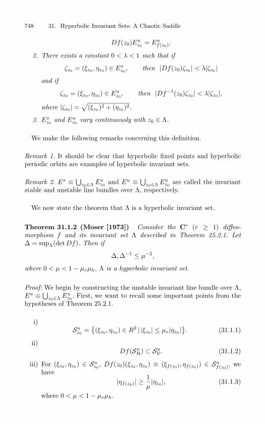
748 31. Hyperbolic Invariant Sets: A Chaotic Saddle
Df(z0)Euz0
= Euf(z0).
2. There exists a constant 0 < λ < 1 such that if
ζz0 = (ξz0 , ηz0) ∈ Esz0
, then |Df(z0)ζz0 | < λ|ζz0 |
and if
ζz0 = (ξz0 , ηz0) ∈ Euz0
, then |Df−1(z0)ζz0 | < λ|ζz0 |,
where |ζz0 | =√
(ξz0)2 + (ηz0)2.
3. Esz0
and Euz0
vary continuously with z0 ∈ Λ.
We make the following remarks concerning this definition.
Remark 1. It should be clear that hyperbolic fixed points and hyperbolicperiodic orbits are examples of hyperbolic invariant sets.
Remark 2. Es ≡⋃
z0∈Λ Esz0
and Eu ≡⋃
z0∈Λ Euz0
are called the invariantstable and unstable line bundles over Λ, respectively.
We now state the theorem that Λ is a hyperbolic invariant set.
Theorem 31.1.2 (Moser [1973]) Consider the Cr (r ≥ 1) diffeo-
morphism f and its invariant set Λ described in Theorem 25.2.1. Let
∆ = supΛ(det Df). Then if
∆, ∆−1 ≤ µ−2,
where 0 < µ < 1− µvµh, Λ is a hyperbolic invariant set.
Proof: We begin by constructing the unstable invariant line bundle over Λ,Eu ≡
⋃z0∈Λ Eu
z0. First, we want to recall some important points from the
hypotheses of Theorem 25.2.1.
i)Su
z0=
(ξz0 , ηz0) ∈ R2 | |ξz0 | ≤ µv|ηz0 |
. (31.1.1)
ii)Df(Su
H) ⊂ SuV . (31.1.2)
iii) For (ξz0 , ηz0) ∈ Suz0
, Df(z0)(ξz0 , ηz0) ≡ (ξf(z0), ηf(z0)) ∈ Suf(z0), we
have|ηf(z0)| ≥
1µ|ηz0 |, (31.1.3)
where 0 < µ < 1− µvµh.
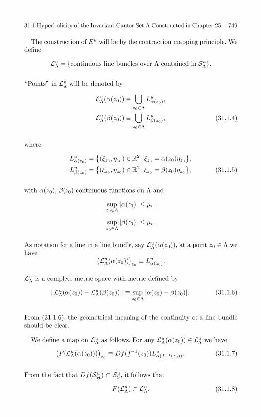
31.1 Hyperbolicity of the Invariant Cantor Set Λ Constructed in Chapter 25 749
The construction of Eu will be by the contraction mapping principle. Wedefine
LuΛ = continuous line bundles over Λ contained in Su
Λ.
“Points” in LuΛ will be denoted by
LuΛ(α(z0)) ≡
⋃z0∈Λ
Luα(z0),
LuΛ(β(z0)) ≡
⋃z0∈Λ
Luβ(z0), (31.1.4)
where
Luα(z0) =
(ξz0 , ηz0) ∈ R
2 | ξz0 = α(z0)ηz0
,
Luβ(z0) =
(ξz0 , ηz0) ∈ R
2 | ξz0 = β(z0)ηz0
, (31.1.5)
with α(z0), β(z0) continuous functions on Λ and
supz0∈Λ
|α(z0)| ≤ µv,
supz0∈Λ
|β(z0)| ≤ µv.
As notation for a line in a line bundle, say LuΛ(α(z0)), at a point z0 ∈ Λ we
have (Lu
Λ(α(z0)))z0≡ Lu
α(z0).
LuΛ is a complete metric space with metric defined by
‖LuΛ(α(z0))− Lu
Λ(β(z0))‖ ≡ supz0∈Λ
|α(z0)− β(z0)|. (31.1.6)
From (31.1.6), the geometrical meaning of the continuity of a line bundleshould be clear.
We define a map on LuΛ as follows. For any Lu
Λ(α(z0)) ∈ LuΛ we have(
F (LuΛ(α(z0)))
)z0≡ Df(f−1(z0))Lu
α(f−1(z0)). (31.1.7)
From the fact that Df(SuH) ⊂ Su
V , it follows that
F (LuΛ) ⊂ Lu
Λ. (31.1.8)
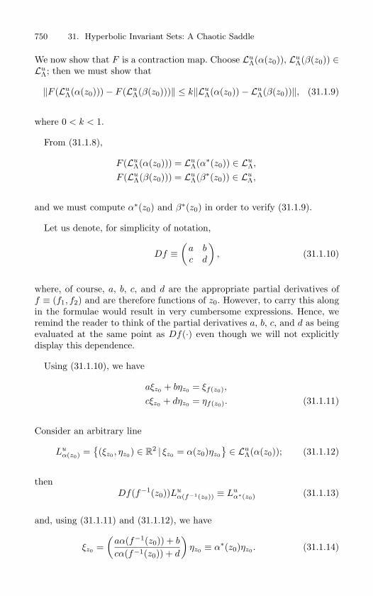
750 31. Hyperbolic Invariant Sets: A Chaotic Saddle
We now show that F is a contraction map. Choose LuΛ(α(z0)), Lu
Λ(β(z0)) ∈Lu
Λ; then we must show that
‖F (LuΛ(α(z0)))− F (Lu
Λ(β(z0)))‖ ≤ k‖LuΛ(α(z0))− Lu
Λ(β(z0))‖, (31.1.9)
where 0 < k < 1.
From (31.1.8),
F (LuΛ(α(z0))) = Lu
Λ(α∗(z0)) ∈ LuΛ,
F (LuΛ(β(z0))) = Lu
Λ(β∗(z0)) ∈ LuΛ,
and we must compute α∗(z0) and β∗(z0) in order to verify (31.1.9).
Let us denote, for simplicity of notation,
Df ≡(
a bc d
), (31.1.10)
where, of course, a, b, c, and d are the appropriate partial derivatives off ≡ (f1, f2) and are therefore functions of z0. However, to carry this alongin the formulae would result in very cumbersome expressions. Hence, weremind the reader to think of the partial derivatives a, b, c, and d as beingevaluated at the same point as Df(·) even though we will not explicitlydisplay this dependence.
Using (31.1.10), we have
aξz0 + bηz0 = ξf(z0),
cξz0 + dηz0 = ηf(z0). (31.1.11)
Consider an arbitrary line
Luα(z0) =
(ξz0 , ηz0) ∈ R
2 | ξz0 = α(z0)ηz0
∈ Lu
Λ(α(z0)); (31.1.12)
thenDf(f−1(z0))Lu
α(f−1(z0)) ≡ Luα∗(z0) (31.1.13)
and, using (31.1.11) and (31.1.12), we have
ξz0 =(
aα(f−1(z0)) + b
cα(f−1(z0)) + d
)ηz0 ≡ α∗(z0)ηz0 . (31.1.14)
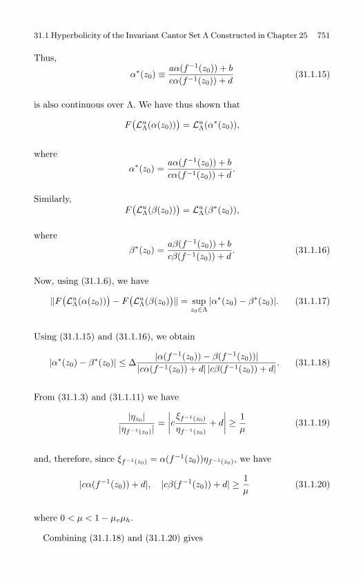
31.1 Hyperbolicity of the Invariant Cantor Set Λ Constructed in Chapter 25 751
Thus,
α∗(z0) ≡aα(f−1(z0)) + b
cα(f−1(z0)) + d(31.1.15)
is also continuous over Λ. We have thus shown that
F(Lu
Λ(α(z0)))
= LuΛ(α∗(z0)),
where
α∗(z0) =aα(f−1(z0)) + b
cα(f−1(z0)) + d.
Similarly,F(Lu
Λ(β(z0)))
= LuΛ(β∗(z0)),
where
β∗(z0) =aβ(f−1(z0)) + b
cβ(f−1(z0)) + d. (31.1.16)
Now, using (31.1.6), we have
‖F(Lu
Λ(α(z0)))− F
(Lu
Λ(β(z0))‖ = sup
z0∈Λ|α∗(z0)− β∗(z0)|. (31.1.17)
Using (31.1.15) and (31.1.16), we obtain
|α∗(z0)− β∗(z0)| ≤ ∆|α(f−1(z0))− β(f−1(z0))|
|cα(f−1(z0)) + d| |cβ(f−1(z0)) + d| . (31.1.18)
From (31.1.3) and (31.1.11) we have
|ηz0 ||ηf−1(z0)|
=∣∣∣∣c ξf−1(z0)
ηf−1(z0)+ d
∣∣∣∣ ≥ 1µ
(31.1.19)
and, therefore, since ξf−1(z0) = α(f−1(z0))ηf−1(z0), we have
|cα(f−1(z0)) + d|, |cβ(f−1(z0)) + d| ≥ 1µ
(31.1.20)
where 0 < µ < 1− µvµh.
Combining (31.1.18) and (31.1.20) gives
752 31. Hyperbolic Invariant Sets: A Chaotic Saddle
|α∗(z0)− β∗(z0)| ≤ µ2∆|α(f−1(z0))− β(f−1(z0))|. (31.1.21)
Note that since Λ is invariant under f , we have
supz0∈Λ
|α(f−1(z0))− β(f−1(z0))| = supz0∈Λ
|α(z0)− β(z0)|. (31.1.22)
Taking the supremum of (31.1.21) over z0 ∈ Λ and using (31.1.22), (31.1.6),and (31.1.17) gives
‖F(Lu
Λ(α(z0)))− F
(Lu
Λ(β(z0)))‖
≤ µ2∆‖LuΛ(α(z0))− Lu
Λ(β(z0))‖; (31.1.23)
thus F is a contraction map provided
µ2∆ < 1. (31.1.24)
Therefore, by the contraction mapping principle, F has a unique, continu-ous fixed point. We denote this fixed point by
Eu =⋃
z0∈Λ
Euz0
. (31.1.25)
Thus we haveF (Eu) = Eu
or, from (31.1.13),
(F (Eu))z0 = Df(f−1(z0))Euf−1(z0) = Eu
z0,
which is what we wanted to construct. The construction of the stable linebundle over Λ is virtually identical and we leave it as an exercise for thereader.
This shows that Λ satisfies Part 1 of Definition 31.1.1. Part 3 followsfrom continuity of the fixed point of F (by the contraction mapping prin-ciple). Continuity is measured with respect to the metric (31.1.6) so thegeometrical meaning should be clear. Part 2 of Definition 31.1.1, expansionand contraction rates, is a trivial consequence of Assumption 3 that weleave as an exercise for the reader.
31.1 Hyperbolicity of the Invariant Cantor Set Λ Constructed in Chapter 25 753
31.1a Stable and Unstable Manifolds of theHyperbolic Invariant Set
Theorem 31.1.2 gives us information on the linearization of f at each pointof Λ, but we can also obtain information on f itself. Recall from the proofof Theorem 25.2.1 that
Λ = Λ−∞ ∩ Λ∞,
withΛ−∞ =
⋃s−i∈S
i=1,2,···
Vs−1···s−k··· ,
Λ∞ =⋃
si∈Si=0,1,···
Hs0···sk··· ,
where, for each infinite sequence of elements of S, Vs−1···s−k··· and Hs0···sk···are µv-vertical and µh-horizontal curves, respectively, with 0 ≤ µvµh < 1.Thus, for any z0 ∈ Λ, there exists a unique µv-vertical curve in Λ−∞,Vs−1···s−k···, and a unique µh-horizontal curve in Λ∞, Hs0···sk···, such that
z0 = Vs−1···s−k··· ∩Hs0···sk···.
Moreover, we can prove the following theorem.
Theorem 31.1.3 (Moser [1973]) Consider the Cr (r ≥ 1) diffeo-
morphism f and its invariant set Λ described in Theorem 25.2.1. Let
∆ = supΛ(det Df). Then if
0 < µ ≤ min
(√|∆|, 1√
|∆|
),
the curves in Λ−∞ and Λ∞ are C1 curves whose tangents at points in Λcoincide with Eu and Es, respectively.
Proof: The proof follows the same ideas as Theorem 31.1.2; in Exercise 2we outline the steps one must complete to establish the theorem.
In some sense we can think of these curves as defining the stable andunstable manifolds of points in Λ. The details of this are worked out in theexercises. But first we must first give some definitions. We will give thesedefinitions in the general n-dimensional setting.
754 31. Hyperbolic Invariant Sets: A Chaotic Saddle
31.2 Hyperbolic Invariant Sets in Rn
Consider a Cr (r ≥ 1) diffeomorphism
f : Rn → R
n,
and let Λ be a compact invariant set for f .
Definition 31.2.1 (Hyperbolic Invariant Set) Λ is said to be a hyper-bolic invariant set if for each p ∈ Λ there is a splitting
Rn = Es
p + Eup ,
which varies continuously with p ∈ Λ, and constants C > 0, 0 < λ < 1such that
1. (Invariance of the Splitting)
Df(p)Esp = Es
f(p),
Df(p)Eup = Eu
f(p).
2. (Contraction and Expansion)
|Dfn(p)v| ≤ Cλn|v|, ∀ v ∈ Esp, p ∈ Λ,
|Df−n(p)v| ≤ Cλn|v|, ∀ v ∈ Eup , p ∈ Λ.
For any point p ∈ Λ, ε > 0, the stable and unstable sets of p of size ε aredefined as follows
W sε (p) =
p′ ∈ Λ | |fn(p)− fn(p′)| ≤ ε for n ≥ 0
,
Wuε (p) =
p′ ∈ Λ | |f−n(p)− f−n(p′)| ≤ ε for n ≥ 0
.
From Chapter 3, we have seen that if p is a hyperbolic fixed point thefollowing hold.
1. For ε sufficiently small, W sε (p) is a Cr manifold tangent to Es
p at pand having the same dimension as Es
p. W sε (p) is called the local stable
manifold of p.
31.2 Hyperbolic Invariant Sets in Rn 755
2. The stable manifold of p is defined as follows
W s(p) =∞⋃
n=0
f−n(W sε (p)).
Similar statements hold for Wuε (p).
The invariant manifold theorem for hyperbolic invariant sets (see Hirsch,Pugh, and Shub [1977]) tells us that a similar structure holds for each pointin Λ.
Theorem 31.2.2 Let Λ be a hyperbolic invariant set of a Cr (r ≥ 1)diffeomorphism f . Then, for ε > 0 sufficiently small and for each point
p ∈ Λ, the following hold.
i) W sε (p) and Wu
ε (p) are Cr manifolds tangent to Esp and Eu
p , respec-
tively, at p and having the same dimension as Esp and Eu
p , respectively.
ii) There are constants C > 0, 0 < λ < 1, such that if p′ ∈ W sε (p), then
|fn(p)− fn(p′)| ≤ Cλn|p− p′|, for n ≥ 0
and if p′ ∈ Wuε (p), then
|f−n(p)− f−n(p′)| ≤ Cλn|p− p′| for n ≥ 0.
iii)
f(W sε (p)) ⊂W s
ε (f(p)),f−1(Wu
ε (p)) ⊂Wuε (f−1(p)).
iv) W sε (p) and Wu
ε (p) vary continuously with p.
Proof: See Hirsch, Pugh, and Shub [1977].
With Theorem 31.2.2 in hand, one can then define the global stable andunstable manifolds of any point p ∈ Λ as follows
W s(p) =∞⋃
n=0
f−n(W sε (fn(p))),
Wu(p) =∞⋃
n=0
fn(Wuε (f−n(p))).
756 31. Hyperbolic Invariant Sets: A Chaotic Saddle
We refer the reader to the exercises for more detailed studies of the issuesraised here in the context of the hyperbolic invariant set constructed inTheorem 31.1.2 and we end this section with some final remarks.
Remark 1: Structural Stability. Hyperbolic invariant sets (like hyperbolicfixed points and periodic orbits) are structurally stable; see Hirsch, Pugh,and Shub [1977].
Remark 2: History. The reason for discussing the concept of hyperbolicinvariant sets is that they have played a central role in the developmentof modern dynamical systems theory. The definitions of Anosov diffemor-phisms and Axiom A diffeomorphisms rely crucially on hyperbolicity, andtheir study has been important for the development of many concepts andtheorems in dynamical systems theory. For example, the ideas of Markovpartitions, pseudo orbits, shadowing, etc., were all developed initially inthese contexts and all utilize crucially the notion of a hyperbolic invariantset1.
Indeed, the existence of a hyperbolic invariant set is often assumed apriori. This has caused the applied scientist great difficulty since, in orderto utilize many of the techniques or theorems of dynamical systems theory,he or she must first show that the system under study possesses a hyperbolicinvariant set. The techniques developed here, specifically the preservation ofsector bundles, allow one to explicitly construct hyperbolic invariant sets.For more information on the consequences and utilization of hyperbolicinvariant sets see Smale [1967], Nitecki [1971], [1978], Conley [1978], Palisand de Melo [1982], Shub [1987], Franks [1982], Palis and Takens [1993],and Katok and Hasselblatt [1995].
Remark 3: Chaotic Saddles. Hyperbolic invariant sets were studied in greatdetail in the 1960’s; well before the term “chaos” was popularized in thecontext of dynamics. Hyperbolic invariant sets are examples of chaotic sad-
dles; a notion around which many papers have been published over the past10 years. See, for example, Lai et al. [1993], Thompson et al. [1994], Ashwinet al. [1996], Dhamala and Lai [1999], Kapitaniak et al. [1999], Kapitaniak[2001], and Robert et. al [1998], [2000]. Most of these works are numericalin nature and fail to recognize the related pioneering work of the 60’s and70’s. Much can be learned about “chaotic saddles” by studying the semi-nal works of Bowen [1970a,b], [1972], [1973], [1975a] and Newhouse [1972].
1Anosov diffeomorphisms are those where the entire phase space is a hyper-bolic invariant set for the diffeomorphism. Axiom A diffeomorphisms are thosehaving the property that their set of nonwandering points (cf. Definition 8.1.5)is hyperbolic and the the set of nonwandering points is the closure of the set ofperiodic orbits.
31.2 Hyperbolic Invariant Sets in Rn 757
Nevertheless, the numerical studies of the last 10 years on chaotic saddlesdo go beyond the previous work in that they consider the more complexissues of loss of hyperbolicity and bifurcation. This is an important area ofresearch for which there are not many theorems, at the moment.
31.2a Sector Bundles for Maps on Rn
In this section we state the higher dimensional analog of Theorem 31.1.2.As above, let f : Rn → R
n be a Cr (r ≥ 1) diffeomorphism and let Λ bea closed set which is invariant under f . Let R
n = Esp ⊕Eu
p be a splittingof R
n for p ∈ Λ and let µ(p) be a positive real valued function defined onΛ. We define the µ(p) sector, denoted Sµ(p), as follows
Sµ(p) =
(ξp, ηp) ∈ Esp ⊕ Eu
p | |ξp| ≤ µ(p) |ηp|
(31.2.1)
and we define the complementary sector, S′µ(p), as follows
S′µ(p) = R
n − Sµ(p). (31.2.2)
Then we have the following theorem.
Theorem 31.2.3 Let f : Rn → Rn be a Cr (r ≥ 1) diffeomorphism
and let Λ ⊂ Rn be a closed set which is invariant under f . Then Λ is a
hyperbolic invariant set if and only if there exists a splitting Rn = Es
p⊕Eup
for each p ∈ Λ, an integer n > 0, constants C > 0, 0 < λ < 1 with
Cλn < 1, and a real valued function µ: Λ → R+ such that the following
conditions are satisfied:
1)supp∈Λ
max(µ(p), µ(p)−1)
< ∞. (31.2.3)
2) For each p ∈ Λ, we have
a) Dfn(p) · Sµ(p) ⊂ Sµ(fn(p))
b) if ξp ∈ S′µ(p), |Dfn(p)ξp| ≤ Cλn |ξp|
c) if ξp ∈ Sµ(p),∣∣Df−n(p)ξp
∣∣ ≤ Cλn |ξp| . (31.2.4)
The proof of this theorem can be found in Newhouse and Palis [1973].Theorem 31.2.3 tells us that in order to establish hyperbolicity for Λ we
758 31. Hyperbolic Invariant Sets: A Chaotic Saddle
need only find bundles of sectors S =⋃
p∈ΛSµ(p), S′ =
⋃p∈Λ
S′µ(p), such that
Df maps S into S while expanding each vector in S and Df maps S′ intoS′ while contracting each vector in S′.
Now regarding Theorem 25.2.1 from Chapter 25, the reader should noticethat if A1 and A3 hold then the invariant set Λ is a hyperbolic invariantset since the conditions of A3 are weakened versions of the necessary andsufficient conditions for a set to be hyperbolic given in Theorem 31.2.3.
31.3 A Consequence of Hyperbolicity: TheShadowing Lemma
We will end this section by discussing the shadowing property associatedwith hyperbolic invariant sets. Two recent monographs on shadowing areLani-Wayda [1995] and Pilyugin [1999]. We follow the proof of Robinson[1977]. First we need some defintions.
Definition 31.3.1 (ε pseudo orbit) An infinite ε pseudo orbit is a dou-
bly infinite sequence of points
xi, | i ∈ ZZ
such that
|f(xi)− xi+1| < ε.
Definition 31.3.2 Suppose U is a neighborhood of a hyperbolic invariant
set Λ where the hyperbolic splitting holds. Then we say that U is a set where
f is hyperbolic.
Lemma 31.3.3 (Shadowing Lemma) Let U ∈ Rn be a region where f
is hyperbolic. Given δ > 0 there exists ε > 0 such that if xi, | i ∈ ZZ is an
ε pseudo orbit in U then there exists a unique y such that
|f i(y)− xi| < δ
for all i ∈ ZZ , i.e. every ε pseudo orbit is δ shadowed by an orbit of f .
Proof: Consider a neighborhood U of Λ where f is hyperbolic. Then theinvariant splitting of R
n over Λ (i.e., Rn = Es
x + Eux , x ∈ Λ) extends to an
“almost invariant” splitting” over U .
31.3 A Consequence of Hyperbolicity: The Shadowing Lemma 759
For each x ∈ U consider the disks of radius δ/2 in Esx and Eu
x . Thecartesian product of these disks gives a neighborhood B(x) of x.
For δ sufficiently small, f is close to Df in B(x). Thus, in B(x) thecontraction and expansion properties of f are close to those of Df .
If ε is small enough, and xi | i ∈ ZZ is an ε pseudo orbit in U , thenf(B(xj−1)) stretches across B(xj) in the unstable directions and is con-tracted in the stable directions. Then f (f (B(xj−1)) ∩B(xj−1))∩B(xj) isan even thinner strip that crosses B(xj) in the unstable directions. Con-tinuing this construction:⋂
n≥0
fn (B(xj−n)) ≡ Du(xj , xi)
is a disk that stretches across B(xj) in the unstable direction. We call it the
unstable disk at xj for the ε pseudo orbit. It does not necessarily containxj and it is the same dimension as Eu
xj.
By construction, a point y ∈ Du(xj , xi) if and only if y ∈ fn (B(xj−n))for all n ≥ 0, i.e., f−n(y) ∈ B(xj−n) for all n ≥ 0. This gives the ”backwardhalf” of the shadowing orbit. Next we construct the ”forward half”.
From the stable manifold theorem it follows that Du(xj , xi) is C1
and almost tangent to Euxj
. Moreover, f expands Du(xj , xi) acrossDu(xj+1, xi). Thus f−1 : Du(xj+1, xi) → Du(xj , xi) is a uniformcontraction. Hence, the contraction mapping principle implies that⋂
n≥0
f−n (Du(xn, xi 0)
,
is the unique point y such that y ∈ f−n(B(xn)) for all n, i.e. such thatfn(y) ∈ B(xn) for all n. Hence, the orbit of y δ shadows the ε pseudoorbit.
31.3a Applications of the Shadowing Lemma
Applications of the shadowing lemma present themselves immediately. Inmany settings our dynamical systems are not “perfect”. The imperfectioncan arise from modelling errors or uncertainties. They could arise in theprocess of numerical simulation of the trajectories of a dynamical systemthrough round-off errors. In each of these situations we would like to knowthat the trajectories of our “approximate” dynamical system are “close”
760 31. Hyperbolic Invariant Sets: A Chaotic Saddle
to a trajectory of the “real” dynamical system. The shadowing lemmaprovides a compelling framework for thinking about such issues. Resultsalong these lines can be found in Nusse and Yorke [1988], Grebogi et al.
[1990], Coomes et al. [1993], [1994a,b], [1995a, b], [1997], Coomes [1997],Palmer [1996], Sauer et al. [1997], Stoffer and Palmer [1999], van Vleck[1995], [2000], Corless [1992], Fryska and Zohdy [1992], Sauer and Yorke[1991], and Palmore and McCauley [1987].
However, it must be understood that shadowing only rigorously holdsin the setting of hyperbolic dynamics–a setting the is extremely rare inapplications. Numerical simulations on the effect of the loss of hyperbolicityon shadowing can be found in Dawson et al. [1994]. A rigorous result hasrecently been obtained by Bonatti et al. [2000].
Applications of shadowing in partial differential equations can be foundin Larsson and Sanz-Serna [1999], Ostermann and Palencia [2000], An-genent [1987], and Chow et al. [1989].
Applications of shadowing in perturbation theory can be found in Mur-dock [1990], [1995], [1996], and Lin [1989], [1996].
Applications of shadowing in fluid mechanics can be found in Klapper[1992], [1993] and Ghosh et al. [1998].
An application of shadowing to predictability can be found in Pearson[2001].
A shadowing lemma for random maps is developed in Chow and vanVleck [1992/93].
Alternate proofs of the shadowing lemma can be found in Meyer and Sell[1987], Feckan [1991], and Hadeler [1996].
Other interesting references concerning shadowing are Chu and Koo[1996], Henry [1994], Kruger and Troubetzkoy [1992], Blank [1991], Stein-lein and Walther [1991], and Palmer [1988].
31.4 Exercises
1. Recall from the proof of Theorem 31.1.2 that
LuΛ =
continuous line bundles over Λ contained in Su
Λ
with typical “points” in Lu
Λ denoted by
LuΛ(α(z0)) ≡
⋃z0∈Λ
Luα(z0),
31.4 Exercises 761
LuΛ(β(z0)) ≡
⋃z0∈Λ
Luβ(z0),
where
Luα(z0) =
(ξz0 , ηz0 ) ∈ R
2 | ξz0 = α(z0)ηz0
,
Luβ(z0) =
(ξz0 , ηz0 ) ∈ R
2 | ξz0 = β(z0)ηz0
.
We defined a metric on LuΛ as follows
‖LuΛ(α(z0)) − Lu
Λ(β(z0))‖ = supz0∈Λ
|α(z0) − β(z0)|. (31.4.1)
a) Prove that (31.4.1) is indeed a metric.
b) Prove that LuΛ is a complete metric space with the metric (31.4.1).
c) Recall the unstable invariant line bundle constructed in Theorem 31.1.2 that wedenoted
Eu =
⋃z0∈Λ
Euz0
.
For ζz0 = (ξz0 , ηz0 ) ∈ Euz0
prove that
|Df−1(z0)ζz0 | < λ|ζz0 |
where 0 < λ < 1.
2. Prove Theorem 31.1.3. Hints: 1) show that the map F defined on LuΛ in (31.1.7) can
be extended to a map on line bundles over Λ−∞ (the µv-vertical curves) and not justΛ.
2) Next, let the graph of x = v(y) be a µv-vertical curve in Λ−∞ and let z0 = (x0, y0)be a point on that curve. Let Tz0 denote the set of lines ξ = α(z0)η with
α(z0) = limn→∞
v(yn) − v(y′n)
yn − y′n
,
where yn = y′n are two sequences approaching y0 for which this limit exists. Show that
|α(z0)| ≤ µv and that the set of α(z0), z0 fixed, satisfying this is closed.
3) Letω(Tz0 ) = max α(z0) − min α(z0) ≤ 2µv,
where the maximum and minimum is taken over the set defined above. Show that ifω(Tz0 ) = 0, then the curve has a derivative at z0 and that, since the two sequences,yn and y′
n, were arbitrary, the derivative is continuous.
4) Finally, we will be through if, from Step 3, we show that ω(Tz0 ) = 0. This is done asfollows. First show that F (Tz0 ) = Tz0 , z0 ∈ Λ−∞, by using the mean value theorem.Next use the contraction property to show that ω(Tz0 ) = ω(F (Tz0 )) ≤ 1
2 ω(Tz0 ) andfrom this conclude that ω(Tz0 ) = 0. Does it follow that Eu
z0agrees with the tangent
to this C1 curve?
If you need help see Moser [1973].
3. Consider the invariant set Λ constructed in Theorem 25.2.1. Using Theorems 31.1.2,31.1.3, and 31.2.2 describe in detail the stable and unstable manifolds of Λ.
4. Horseshoes are Structurally Stable. Suppose that a map f : D → R2 satisfies the
hypothesis of Theorem 25.2.1. Then it possesses an invariant Cantor set Λ. Show that,for ε sufficiently small, the map f + εg (with g Cr, r ≥ 1, on D) also possesses an
invariant Cantor set Λε. Moreover, show that Λε can be constructed so that (f +εg)∣∣∣Λε
is topologically conjugate to f∣∣∣Λ.
32
Long Period Sinks inDissipative Systems andElliptic Islands in ConservativeSystems
Long period sinks in dissipative systems and elliptic islands in conservativesystems are the “demons” that thwart proofs of the existence of strangeattractors in dissipative systems and sets of positive measure on which thedynamics is chaotic in conservative systems. In this chapter we describesome aspects of these phenomena.
32.1 Homoclinic Bifurcations: Cascades ofPeriod-Doubling and Saddle-NodeBifurcations
In Chapter 26 we described some aspects of the complex dynamics asso-ciated with a transverse homoclinic orbit to a hyperbolic fixed point. Inparticular, the map possessed a countable infinity of unstable periodic or-bits of all periods. We now want to consider the situation of a bifurcationto transverse homoclinic orbits. Specifically, we consider a one-parameterfamily of diffeomorphisms of the plane having a hyperbolic periodic orbit(which, without loss of generality, we can assume is a fixed point). Refer-ring to the parameter as µ, suppose, for µ > µ0, the stable and unstablemanifolds of the fixed point do not intersect and, for µ < µ0, they intersecttransversely (the reader might peek ahead to Figure 32.1.2). Hence, a nat-ural question arises; as we go from µ > µ0 (i.e., no horseshoe) to µ < µ0(i.e., many horseshoes), how are all the unstable periodic orbits created?We will see that under certain conditions the creation of the complicateddynamics associated with a transverse homoclinic orbit to a hyperbolicperiodic orbit is an infinite sequence (or cascade) of period-doubling andsaddle-node bifurcations. The set-up for the analysis will be very similar
32.1 Homoclinic Bifurcations 763
to that given in Chapter 26 for the proof of Moser’s theorem. Specifically,we will analyze a sufficiently large iterate of the map that is defined in aneighborhood (in both phase and parameter space) of a homoclinic point.We begin by stating our assumptions.
We consider a one-parameter family of two-dimensional Cr (r ≥ 3) dif-feomorphisms
z → f(z;µ), z ∈ R2, µ ∈ I ⊂ R
1, (32.1.1)
where I is some interval in R1. We have the following assumption on the
map.
Assumption 1: Existence of a Hyperbolic Fixed Point. For all µ ∈ I,
f(0, µ) = 0. (32.1.2)
Moreover, z = 0 is a hyperbolic fixed point with the eigenvalues of Df(0, µ)given by ρ(µ), λ(µ), with
0 < ρ(µ) < 1 < λ(µ) <1
ρ(µ). (32.1.3)
We remark that since (32.1.3) is satisfied for all µ ∈ I, we will often omitdenoting the explicit dependence of the eigenvalues ρ and λ on µ unless itis relevant to the specific argument being discussed. We denote the stableand unstable manifolds of the hyperbolic fixed point by W s
µ(0) and Wuµ (0),
respectively.
Assumption 2: Existence of a Homoclinic Point. At µ = 0, W s0 (0) and
Wu0 (0) intersect.
Assumption 3: Behavior Near the Fixed Point. There exists some neigh-borhood N of the origin such that the map takes the form
f(x, y; µ) = (ρx, λy), (32.1.4)
where x and y are local coordinates in N .
Note that Assumption 3 implies that W sµ(0) ∩ N and Wu
µ (0) ∩ N aregiven by the local coordinate axes.
Our final assumption will place more specific conditions on the geometryof the intersection of W s
µ(0) with Wuµ (0) at µ = 0. This is most conveniently
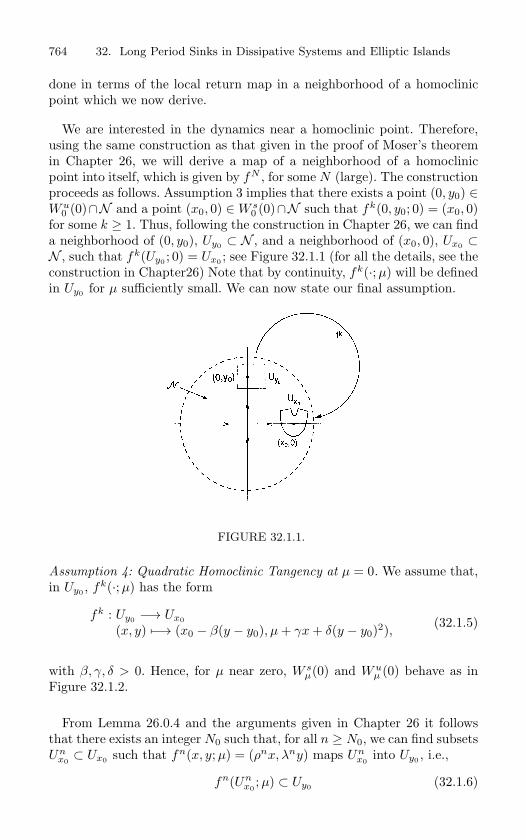
764 32. Long Period Sinks in Dissipative Systems and Elliptic Islands
done in terms of the local return map in a neighborhood of a homoclinicpoint which we now derive.
We are interested in the dynamics near a homoclinic point. Therefore,using the same construction as that given in the proof of Moser’s theoremin Chapter 26, we will derive a map of a neighborhood of a homoclinicpoint into itself, which is given by fN , for some N (large). The constructionproceeds as follows. Assumption 3 implies that there exists a point (0, y0) ∈Wu
0 (0)∩N and a point (x0, 0) ∈ W s0 (0)∩N such that fk(0, y0; 0) = (x0, 0)
for some k ≥ 1. Thus, following the construction in Chapter 26, we can finda neighborhood of (0, y0), Uy0 ⊂ N , and a neighborhood of (x0, 0), Ux0 ⊂N , such that fk(Uy0 ; 0) = Ux0 ; see Figure 32.1.1 (for all the details, see theconstruction in Chapter26) Note that by continuity, fk(·;µ) will be definedin Uy0 for µ sufficiently small. We can now state our final assumption.
FIGURE 32.1.1.
Assumption 4: Quadratic Homoclinic Tangency at µ = 0. We assume that,in Uy0 , fk(·;µ) has the form
fk : Uy0 −→ Ux0
(x, y) −→ (x0 − β(y − y0), µ + γx + δ(y − y0)2),(32.1.5)
with β, γ, δ > 0. Hence, for µ near zero, W sµ(0) and Wu
µ (0) behave as inFigure 32.1.2.
From Lemma 26.0.4 and the arguments given in Chapter 26 it followsthat there exists an integer N0 such that, for all n ≥ N0, we can find subsetsUn
x0⊂ Ux0 such that fn(x, y;µ) = (ρnx, λny) maps Un
x0into Uy0 , i.e.,
fn(Unx0
; µ) ⊂ Uy0 (32.1.6)
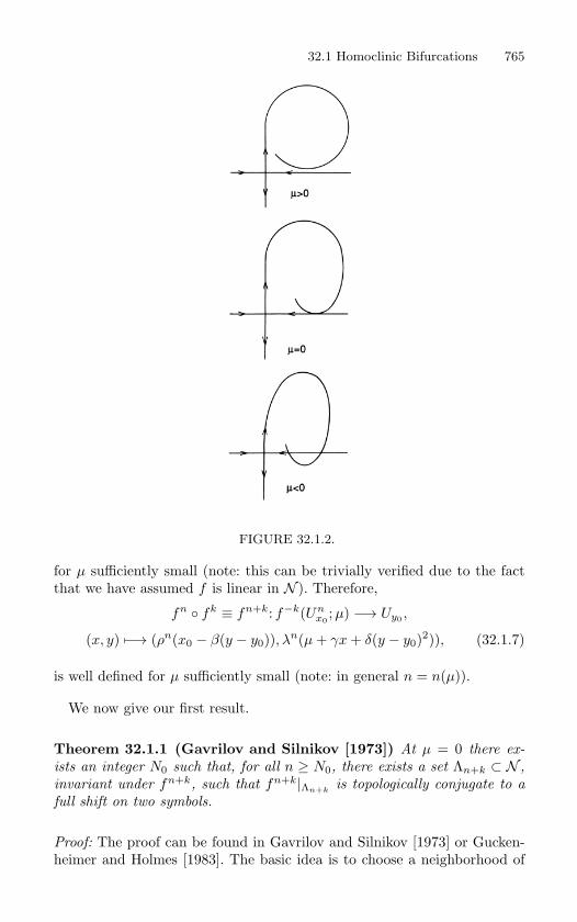
32.1 Homoclinic Bifurcations 765
FIGURE 32.1.2.
for µ sufficiently small (note: this can be trivially verified due to the factthat we have assumed f is linear in N ). Therefore,
fn fk ≡ fn+k: f−k(Unx0
;µ) −→ Uy0 ,
(x, y) −→ (ρn(x0 − β(y − y0)), λn(µ + γx + δ(y − y0)2)), (32.1.7)
is well defined for µ sufficiently small (note: in general n = n(µ)).
We now give our first result.
Theorem 32.1.1 (Gavrilov and Silnikov [1973]) At µ = 0 there ex-
ists an integer N0 such that, for all n ≥ N0, there exists a set Λn+k ⊂ N ,
invariant under fn+k, such that fn+k|Λn+kis topologically conjugate to a
full shift on two symbols.
Proof: The proof can be found in Gavrilov and Silnikov [1973] or Gucken-heimer and Holmes [1983]. The basic idea is to choose a neighborhood of
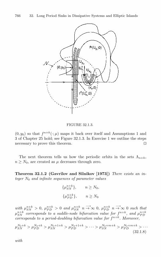
766 32. Long Period Sinks in Dissipative Systems and Elliptic Islands
FIGURE 32.1.3.
(0, y0) so that fn+k(·;µ) maps it back over itself and Assumptions 1 and3 of Chapter 25 hold; see Figure 32.1.3. In Exercise 1 we outline the stepsnecessary to prove this theorem.
The next theorem tells us how the periodic orbits in the sets Λn+k,n ≥ N0, are created as µ decreases through zero.
Theorem 32.1.2 (Gavrilov and Silnikov [1973]) There exists an in-
teger N0 and infinite sequences of parameter values
µn+kSN , n ≥ N0,
µn+kPD , n ≥ N0
with µn+kSN > 0, µn+k
PD > 0 and µn+kSN
−→n →∞ 0, µn+k
PD
−→n →∞ 0 such that
µn+kSN corresponds to a saddle-node bifurcation value for fn+k, and µn+k
PD
corresponds to a period-doubling bifurcation value for fn+k. Moreover,
µN0+kSN > µN0+k
PD > µN0+1+kSN > µN0+1+k
PD > · · · > µN0+m+kSN > µN0+m+k
PD > · · ·(32.1.8)
with
32.1 Homoclinic Bifurcations 767
µn+kSN ∼ λ−n as n →∞ (32.1.9)
and
µn+kPD ∼ λ−n as n →∞. (32.1.10)
Before proving Theorem 32.1.2 we want to make several remarks.
Remark 1. In the saddle-node bifurcation at µ = µn+kSN , the node is actually
a sink. The two orbits created are period n + k orbits for f . The sink cre-ated in the saddle-node bifurcation subsequently loses stability in a period-doubling bifurcation at µ = µn+k
PD (hence, we must have µn+kPD < µn+k
SN ),resulting in the creation of a period 2(n + k) sink for f . This bifurcationscenario will be verified in the course of the proof of Theorem 32.1.2.
Remark 2. Theorem 32.1.2 tells us how the countable infinity of periodicorbits in the horseshoes for µ ≤ 0 are created; namely, the periodic orbitsare created in saddle-node bifurcations, and the period is increased throughperiod-doubling bifurcations.
Remark 3. Equations (32.1.9) and (32.1.10) gives us the rate by which theperiod-doubling and saddle-node bifurcation values accumulate on µ = 0.This rate is not universal but depends on the size of the unstable eigenvalueof the hyperbolic fixed point.
Remark 4. Theorems 32.1.1 and 32.1.2 are stated explicitly for dissipativeor nonconservative maps, i.e., λρ < 1. However, similar results will holdfor area-preserving maps where we have λρ = 1; see Newhouse [1983] andExercise 3.
We now begin the proof of Theorem 32.1.2.
Proof: The proof is constructive. The condition for fixed points of fn+k isgiven by
x = ρnx0 − βρn(y − y0), (32.1.11)y = µλn + γλnx + δλn(y − y0)2, (32.1.12)
where it is important to recall that x0, y0, γ, β, δ, and ρ > 0. By substi-tuting (32.1.11) into (32.1.12) we obtain
δλny2 − (βγλnρn + 2δλny0 + 1)y + δλny20
+ βγλnρny0 + γρnλnx0 + µλn = 0. (32.1.13)
768 32. Long Period Sinks in Dissipative Systems and Elliptic Islands
Solving (32.1.13) yields
y =βγλnρn + 2δλny0 + 1
2δλn
± 12δλn
[((βγλnρn + 2δλny0 + 1)2 (32.1.14)
− 4δλn(δλny20 + βγλnρny0 + γλnρnx0 + µλn)
]1/2.
After some algebra, the expression under the radical in (32.1.15) can besimplified so that (32.1.15) becomes
y =βγλnρn + 2δλny0 + 1
2δλn± 1
2δλn
×√
4δλ2n[ (βγρn + λ−n)2
4δ+ (y0λ−n − γρnx0)− µ
]. (32.1.15)
Note that (32.1.15) is a function of n and µ. Thus, (32.1.15) gives they coordinate of a fixed point which can be substituted into (32.1.11) toobtain the x coordinate. Note that since (32.1.11) is linear in x, for a fixedy coordinate there is a unique x coordinate for the fixed point. Thus, instudying the numbers of fixed points and their bifurcations, it suffices tostudy only (32.1.15).
From (32.1.15) we can easily see that there are no fixed points for
µ >(βγρn + λ−n)2
4δ+ (y0λ
−n − γρnx0) (32.1.16)
and two fixed points for
µ <(βγρn + λ−n)2
4δ+ (y0λ
−n − γρnx0). (32.1.17)
Therefore,
µ =(βγρn + λ−n)2
4δ+ (y0λ
−n − γρnx0) (32.1.18)
is a bifurcation value for fn+k.
Next, we verify that this is a saddle-node bifurcation. This can be showndirectly. From (32.1.7), the matrix associated with the linearized map isgiven by
32.1 Homoclinic Bifurcations 769
Dfn+k =(
0 −βρn
γλn 2δλn(y − y0)
); (32.1.19)
hence we have
det Dfn+k = γβρnλn, (32.1.20)trDfn+k = 2δλn(y − y0), (32.1.21)
with eigenvalues, χ1 and χ2, of (4.7.17) given by
χ1,2 =trDfn+k
2± 1
2
√(trDfn+k)2 − 4 det Dfn+k. (32.1.22)
At the bifurcation value (32.1.18) there is only one fixed point where, using(32.1.20), (32.1.21), and (32.1.22), the eigenvalues of (32.1.19) are given by
χ1 = 1, χ2 = γβρnλn. (32.1.23)
Note that since ρλ < 1, by taking n sufficiently large, χ2 can be madearbitrarily small.
At this point we want to check the stability of the bifurcating fixed points.From (32.1.20), (32.1.21) and using ρλ < 1, we see that for n sufficientlylarge, the eigenvalues of (32.1.19) are approximately given by
χ1 ≈ trDfn+k, (32.1.24)χ2 ≈ 0, (32.1.25)
and by substituting (32.1.15) into (32.1.21) (and neglecting terms ofO(ρnλn)) we have
χ1 ≈ 1
±√
4δλ2n
((γβρn + λ−n)2
4δ+ (y0λ−n − γx0ρn)− µ
).(32.1.26)
Thus, for the branch of fixed points with y coordinate given by
y =βγλnρn + 2δλny0 + 1
2δλn+
12δλn
×√
4δλ2n
((βγρn + λ−n)2
4δ+ (y0λ−n − γρnx0)− µ
),(32.1.27)
770 32. Long Period Sinks in Dissipative Systems and Elliptic Islands
the eigenvalues associated with the linearized map are, for n sufficientlylarge, approximately given by
χ1 ≈ 1 +
√4δλ2n
((γβρn + λ−n)2
4δ+ (y0λ−n − γx0ρn)− µ
),
χ2 ≈ 0. (32.1.28)
Hence, for
µ <(γβρn + λ−n)2
4δ+ (y0λ
−n − γx0ρn) (32.1.29)
(which, from (32.1.18), is the saddle-node bifurcation value), it is easy tosee that this fixed point is always a saddle. Similarly, for the branch of fixedpoints given by
y =βγλnρn + 2δλny0 + 1
2δλn
− 12δλn
√4δλn
((βγρn + λ−n)2
4δ+ (y0λ−n − γρnx0)− µ
),
(32.1.30)
the eigenvalues associated with the linearized map are, for n sufficientlylarge, approximately given by
χ1 ≈ 1−√
4δλ2n
((βγρn + λ−n)2
4δ+ (y0λ−n − γρnx0)− µ
),
χ2 ≈ 0. (32.1.31)
Therefore, for µ “slightly” less than (βγρn+λ−n)2
4δ + (y0λ−n − γρnx0), it is
easy to see that this fixed point is a sink. However, as µ decreases further, itis possible for χ1 to decrease through −1 and, consequently, for this branchof fixed points to undergo a period-doubling bifurcation. We now want tostudy this possibility.
We are considering the branch of fixed points with y coordinate given by
y =βγλnρn + 2δλny0 + 1
2δλn− 1
2δλn
×√
4δλ2n
((βγρn + λ−n)2
4δ+ (y0λ−n − γρnx0)− µ
).(32.1.32)
32.1 Homoclinic Bifurcations 771
From (32.1.22), the condition for an eigenvalue of Dfn+k to be −1 is
1 + det Dfn+k = −trDfn+k. (32.1.33)
Substituting (32.1.20) and (32.1.21) into (32.1.33) yields
1 + γβρnλn = 2δλny0 − 2δλny, (32.1.34)
and substituting (32.1.32) into (32.1.34) yields
1 + γβρnλn =
√δλ2n
((βγρn + λ−n)2
4δ+ (y0λ−n − γρnx0)− µ
).
(32.1.35)
By solving (32.1.35) for µ, we obtain
µ = − 34δ
(γβρn + λ−n)2 + (y0λ−n − γρnx0). (32.1.36)
Hence, (32.1.36) is the bifurcation value for the period-doubling bifurcationof the sink created in the saddle-node bifurcation. We leave it as an exercisefor the reader to verify that the period-doubling bifurcation is “generic”(see Exercise 2).
Let us summarize what we have shown thus far. The map fn+k, for nsufficiently large, undergoes a saddle-node bifurcation at
µn+kSN =
(βγρn + λ−n)2
4δ+ (y0λ
−n − γρnx0). (32.1.37)
In this bifurcation two fixed points of fn+k are created, a saddle and asink. As µ decreases below µn+k
SN , the saddle remains a saddle but the sinkundergoes a period-doubling bifurcation at
µn+kPD = −3(βγρn + λ−n)2
4δ+ (y0λ
−n − γρnx0). (32.1.38)
It is easy to see from (32.1.37) and (32.1.38) that we have
µn+kPD < µn+k
SN .
Also, for n sufficiently large, we have
y0λ−n − γρnx0 >> (βγρn + λ−n)2. (32.1.39)
772 32. Long Period Sinks in Dissipative Systems and Elliptic Islands
Using (32.1.39) along with the fact that
(y0λ−n − γρnx0) = λ−n(y0 − γρnλnx0) (32.1.40)
with ρλ < 1 implies thatµn+k
SN > 0
andµn+k
PD > 0
for n sufficiently large. Next we need to show that
µn+1+kSN < µn+k
PD .
From (32.1.37) and (32.1.38), we have
µn+1+kSN =
(βγρn+1 − λ−n−1)2
4δ+ λ−n−1(y0 − γρn+1λ−n−1x0) (32.1.41)
and
µn+kPD = −3(βγρn − λ−n)2
4δ+ λ−n(y0 − γρnλnx0). (32.1.42)
Using (32.1.39) and (32.1.40), along with the fact that λ > 1, we can easilysee from (32.1.41) and (32.1.42) that, for n sufficiently large, we have
µn+1+kSN < µn+k
PD . (32.1.43)
Equation (32.1.8) now follows from (32.1.43) by induction. Finally, it fol-lows from (32.1.39), (32.1.37) and (32.1.38) that
µn+kSN ∼ λ−n as n →∞
andµn+k
PD ∼ λ−n as n →∞.
Let us now comment on the generality of our results. In particular, inAssumption 2 we assumed that our map is linear in a neighborhood, N ,of the origin, and in Assumption 3 we assumed that the form of the mapdefined outside of a neighborhood of the origin is given as in (32.1.5). Itfollows from the work of Gavrilov and Silnikov [1972], [1973] that our resultsare not restricted by these assumptions in the sense that if we assume themost general forms for f in N and for fk, Theorems 32.1.1 and 32.1.2 areunchanged. We remark that this generally holds for the study of the orbitstructure near orbits homoclinic to hyperbolic periodic points. A returnmap defined near a homoclinic point constructed as the composition of aniterate of the linearized map near the origin with low-order terms in the
32.1 Homoclinic Bifurcations 773
Taylor expansion of an iterate of the map outside of a neighborhood ofthe origin is sufficient to capture the qualitative dynamics in a sufficientlysmall neighborhood of the homoclinic point. Let us now briefly describethe set-up considered by Gavrilov and Silnikov.
In local coordinates in N , Gavrilov and Silnikov showed that a generalCr (r ≥ 3) diffeomorphism can be written in the form(
xy
)−→
(λ(µ)x + f(x, y; µ)xρ(µ)y + g(x, y;µ)y
). (32.1.44)
For the form of fk acting outside of N (but mapping a neighborhood of ahomoclinic point on the local unstable manifold in N to a neighborhood ofthe local stable manifold in N ), they assumed the completely general form
fk:(
xy
)−→
(x0 + F (x, y − y0;µ)G(x, y − y0;µ)
). (32.1.45)
The assumption of quadratic homoclinic tangency at µ = 0 requires
Gy(0, 0, 0) = 0, (32.1.46)
Gyy(0, 0, 0) = 0 (32.1.47)
(note: since f is a diffeomorphism, then (32.1.46) implies that we must haveGx(0, 0, 0) = 0 and Fy(0, 0, 0) = 0). Gavrilov and Silnikov then simplify(32.1.45) as follows; letting
y − y0 = φ(x, µ) (32.1.48)
be the (unique) solution of
Gy(x, y − y0, µ) = 0 (32.1.49)
(which can be solved by the implicit function theorem as a result of(32.1.47)), (32.1.45) can be rewritten as(
xy
)−→
(x0 + F (x, y − y0;µ)
E(µ) + C(x, µ)x + D(x, µ)(y − y0 − φ(x, µ))2
), (32.1.50)
where
E(µ) ≡ G(0, φ(0, µ), µ), E(0) = 0,C(0, 0) ≡ c,
2D(0, y0, 0) ≡ d.
The reader should note the similarity of (32.1.50) and (32.1.5). The num-bers c and d in (32.1.50) describe the geometry of the tangency of the stable
774 32. Long Period Sinks in Dissipative Systems and Elliptic Islands
and unstable manifolds. Gavrilov and Silnikov show that there are ten casesto consider depending on the signs of λ, ρ, c, and d. (Note: yes, there are16 possible combinations of signs of these parameters, but Gavrilov andSilnikov show how to reduce the number of possibilities.)
Five of the cases correspond to orientation-preserving maps with the re-maining five corresponding to orientation-reversing maps. The example wetreated corresponds to one of the five orientation-preserving maps with λ,ρ, c, d > 0. The structure of the period-doubling and saddle-node cascadescan be different for the remaining cases, and we refer the reader to Gavrilovand Silnikov [1972], [1973] for the details.
32.2 Newhouse Sinks in Dissipative Systems
The following corollary is an obvious consequence of the proof of Theorem32.1.2.
Corollary 32.2.1 Let p0 denote a point of quadratic tangency of W s0 (0)
and Wu0 (0). Then for all n sufficiently large there is a parameter value,
µn+k, with µn+k → 0 as n → ∞, such that f has a periodic sink, pn, of
period n + k with pn → p0 as n →∞.
The reason for pulling out this corollary from Theorem 32.1.2 is that if weput it together with some deep results of Newhouse concerning the persis-tence of quadratic homoclinic tangencies, we get a very provocative result.(Note: Newhouse’s results do not require our more restrictive Assumptions3 and 4 given above but, rather, they apply to any two-dimensional dif-feomorphism having a dissipative hyperbolic periodic point whose stableand unstable manifolds have a quadratic tangency.) We now want to givea brief description of the implications of Newhouse’s results in the contextof this section.
It should be clear that a specific point of tangency of W s0 (0) and Wu
0 (0)can easily be destroyed by the slightest perturbation. However, Newhouse[1974] has proven the following result.
Theorem 32.2.2 For ε > 0, let Iε = µ ∈ I | |µ| < ε. Then, for every
ε > 0, there exists a nontrivial interval Iε ⊂ Iε such that Iε contains a
dense set of points at which W sµ(0) and Wu
µ (0) have a quadratic homoclinic
tangency.
32.2 Newhouse Sinks in Dissipative Systems 775
Proof: This “parametrized” version of Newhouse’s theorem is due to Robin-son [1983].
Heuristically, Theorem 32.2.2 says that if we destroy the quadratic ho-moclinic tangency at µ = 0 by varying µ slightly, then for a dense setof parameter values containing µ = 0, we have a quadratic homoclinictangency somewhere else in the homoclinic tangle. Thus, Corollary 32.2.1can be applied to each of these tangencies so that Corollary 32.2.1 andTheorem 32.2.2 together imply that there are parameter values at whichthe map has infinitely many periodic attractors which coexist with Smalehorseshoe–type dynamics. This phenomenon is at the heart of the diffi-culties encountered in proving that a two-dimensional map possesses a“strange attractor.” We will discuss this in much more detail in Chapter30.
We close with some final remarks.
Remark 1: For higher dimensional generalizations of the Newhouse sinkphenomenon see Palis and Viana [1994].
Remark 2: The Codimension of a Homoclinic Bifurcation. By the term“homoclinic bifurcation,” we mean the creation of transverse homoclinicorbits to a hyperbolic periodic point of a two-dimensional diffeomorphismas parameters are varied. Since the stable and unstable manifolds of the hy-perbolic periodic point are codimension one, their transversal intersectionoccurs stably in a one-parameter family of maps. Now recall the definitionof “codimension of a bifurcation” given in Chapter 20. Roughly speaking,the codimension is the number of parameters in which the correspondingparametrized family is stable under perturbations. We have seen in thissection that there is an infinity of saddle-node and period-doubling bifurca-tion values accumulating on the quadratic homoclinic tangency parametervalue. Thus the type of bifurcation is codimension infinity by the standarddefinitions. In particular, one cannot find a versal deformation for this typeof bifurcation satisfying the standard definitions given in Chapter 20.
Remark 3. There have been a number of papers by the Maryland groupover the last few years that have shed much light on the creation of horse-shoes. In particular, we refer the reader to Yorke and Alligood [1985] andAlligood et al. [1987]. In Tedeschini-Lalli and Yorke [1986] the question ofthe measure of the set of parameter values for which the map possesses aninfinite number of coexisting periodic sinks is addressed. For a “generic”map, the measure of the set is shown to be zero.
776 32. Long Period Sinks in Dissipative Systems and Elliptic Islands
Remark 4. For additional recent work on the dynamical consequences as-sociated with homoclinic tangencies see Diaz et al. [1999], Diaz and Rocha[1997a, b], Diaz [1995] and Diaz and Ures [1994].
32.3 Islands of Stability in Conservative Systems
There is a conservative analog of the Newhouse sink phenomenon. Earlyresults along these lines are due to Newhouse [1977]. An analysis similar inspirit to the Gavrilov and Silnikov work described in this chapter is givenin Gonchenko and Silnikov [2000]. See also Duarte [1999].
32.4 Exercises
1. Prove Theorem 32.1.1. (Hints: the idea is to find a region Sn in Uy0 such that As-sumptions 1 and 3 of Chapter 25 hold for fn+k. 1) Let Sn = (x, y) | |y − y0| ≤ ε,0 ≤ x ≤ νn where ρ < ν < 1
λ . The idea is to show that fn+k(Sn; 0) intersectsSn in two µv-vertical strips. Then the pre-image of these two µv-vertical strips willbe µh-horizontal strips with proper boundary behavior and 0 ≤ µhµv < 1. This canbe accomplished in several steps. First show that under fk(·; 0), vertical lines in Sn
(i.e., lines with x = c = constant) map to parabolas in Ux0 given by the graph ofy = γc+ δ
β2 (x−x0)2. 2) Show that for n sufficiently large, the x-components of points
in fn+k(·; µ) are smaller than νn. 3) Finally, show that for ε = ε(n) ∼ (y0λ−n/δ)1/2,fn+k(Sn; 0) cuts through the top and bottom horizontal boundaries of Sn. From thesethree facts you should be able to find µh-horizontal and µv-vertical strips so that As-sumption 1 is satisfied.
The proof that Assumption 3 holds is very similar to the same step carried out inTheorem 26.0.5. Use the fact that
Dfn+k(x, y; 0) =
(0 −βρn
γλn 2δλn(y − y0)
)
and that, for |y − y0| ∼ (y0λ−n/δ)1/2 and n sufficiently large, this Jacobian is essen-tially
Dfn+k(x, y; 0) ∼
(0 0
γλn 2(y0δλn)1/2
).
(Drawing figures in each case should help.)
2. Recall the proof of Theorem 32.1.2. In showing that the sink created in the saddle-nodebifurcation of fn+k subsequently underwent a period-doubling bifurcation at
µ = − 34δ
(γβρn + λ
−n)2 + (y0λ−n − γρ
nx0),
we only showed that the map had an eigenvalue of −1 at this parameter value. Examinethe nonlinear terms (possibly do a center manifold reduction) to show that this period-doubling bifurcation is indeed nondegenerate or “generic.”
3. Show that Theorem 32.1.2 holds for area-preserving maps. (Hint: use the implicitfunction theorem proof given in Tedeschini-Lalli and Yorke [1986].)
4. Does the result of Theorem 32.1.1 hold for area-preserving maps?
33
Global Bifurcations Arisingfrom Local Codimension—TwoBifurcations
In Section 20.6 we studied the bifurcation of a fixed point of a vectorfield in the situation where the matrix associated with the linearization ofthe vector field at the bifurcation point had two zero eigenvalues, and inSection 20.7 we studied the situation where the matrix had a zero and apure imaginary pair of eigenvalues (with any remaining eigenvalues havingnonzero real part). In both cases we saw that dynamical phenomena arosewhich could not be explained by any local bifurcation analysis, and in thissection we want to attempt to complete the analysis. In the case of thedouble-zero eigenvalue we will succeed completely. In the case of the zero-pure imaginary pair we will only achieve partial success. We begin with thedouble-zero eigenvalue.
33.1 The Double-Zero Eigenvalue
Recall from Section 20.6 that the truncated normal form associated withthis bifurcation is given by
x = y,
y = µ1 + µ2y + x2 + bxy, b = ±1. (33.1.1)
Equation (33.1.1) applies to generic vector fields, i.e., there are no symme-tries and we treat the case b = +1.
Recall that (33.1.1) has no periodic orbits for µ1 > 0 and, for µ1 <0, periodic orbits are created in a Poincare-Andronov-Hopf bifurcation.Therefore, there must be some other bifurcation occurring which accountsfor the destruction of the periodic orbits as µ1 increases through zero. InSection 20.6 we gave some heuristic arguments as to why this should be
778 33. Global Bifurcations
a homoclinic or saddle-connection bifurcation, and now we want to provethis.
We begin by rescaling the dependent variables and parameters of (33.1.1)as follows
x = ε2u, y = ε3v, µ1 = −ε4, µ2 = ε2ν2 (ε > 0), (33.1.2)
and we rescale the independent variable time as follows
t −→ t
ε,
so that (33.1.1) becomes
u = v,
v = −1 + u2 + ε(ν2v + uv). (33.1.3)
Notice that, in the original variables, we are interested in µ1 < 0 and thatour rescaling allows us to interpret our results in this parameter regime.(Note: the reader should be somewhat irritated that we have simply pulledthis particular rescaling “out of the air.” For now, we will proceed with theanalysis, but at the end of this section we will discuss “why it works.”)
The single most important characteristic of this rescaling is that, forε = 0, the rescaled equations (33.1.3) become a completely integrableHamiltonian system with Hamiltonian function given by
H(u, v) =v2
2+ u− u3
3. (33.1.4)
Melnikov’s method can then be used to perform a global analysis thatincludes the effects of the higher order terms of the normal form. Thephase space of this completely integrable Hamiltonian system is shown inFigure 33.1.1. Thus, the vector field
u = v,
v = −1 + u2, (33.1.5)
has a hyperbolic fixed point at
(u, v) = (1, 0),
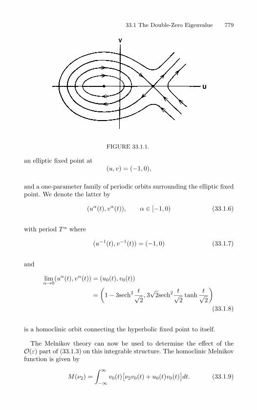
33.1 The Double-Zero Eigenvalue 779
FIGURE 33.1.1.
an elliptic fixed point at(u, v) = (−1, 0),
and a one-parameter family of periodic orbits surrounding the elliptic fixedpoint. We denote the latter by
(uα(t), vα(t)), α ∈ [−1, 0) (33.1.6)
with period Tα where
(u−1(t), v−1(t)) = (−1, 0) (33.1.7)
and
limα→0
(uα(t), vα(t)) = (u0(t), v0(t))
=(
1− 3sech2 t√2, 3√
2sech2 t√2
tanht√2
)(33.1.8)
is a homoclinic orbit connecting the hyperbolic fixed point to itself.
The Melnikov theory can now be used to determine the effect of theO(ε) part of (33.1.3) on this integrable structure. The homoclinic Melnikovfunction is given by
M(ν2) =∫ ∞
−∞v0(t)
[ν2v0(t) + u0(t)v0(t)
]dt. (33.1.9)
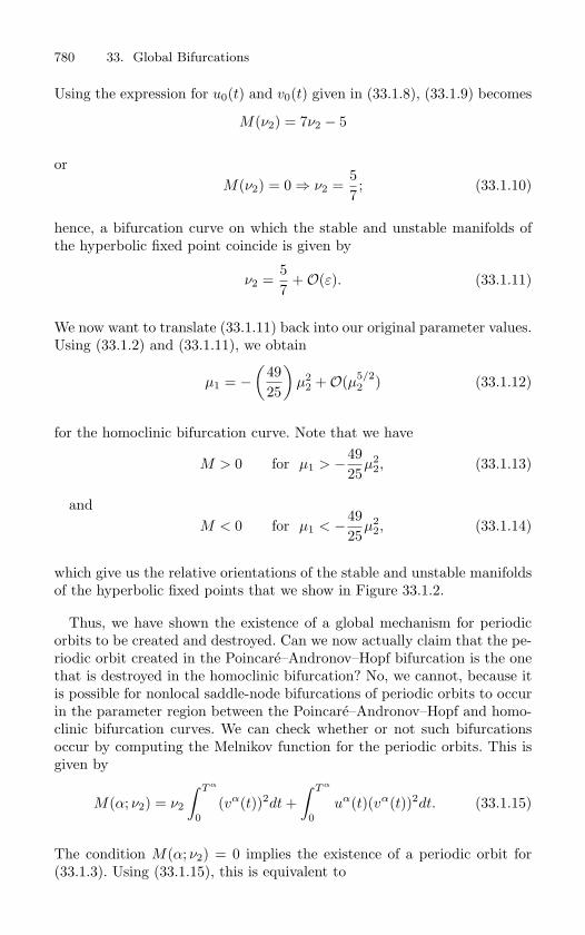
780 33. Global Bifurcations
Using the expression for u0(t) and v0(t) given in (33.1.8), (33.1.9) becomes
M(ν2) = 7ν2 − 5
orM(ν2) = 0 ⇒ ν2 =
57; (33.1.10)
hence, a bifurcation curve on which the stable and unstable manifolds ofthe hyperbolic fixed point coincide is given by
ν2 =57
+O(ε). (33.1.11)
We now want to translate (33.1.11) back into our original parameter values.Using (33.1.2) and (33.1.11), we obtain
µ1 = −(
4925
)µ2
2 +O(µ5/22 ) (33.1.12)
for the homoclinic bifurcation curve. Note that we have
M > 0 for µ1 > −4925
µ22, (33.1.13)
andM < 0 for µ1 < −49
25µ2
2, (33.1.14)
which give us the relative orientations of the stable and unstable manifoldsof the hyperbolic fixed points that we show in Figure 33.1.2.
Thus, we have shown the existence of a global mechanism for periodicorbits to be created and destroyed. Can we now actually claim that the pe-riodic orbit created in the Poincare–Andronov–Hopf bifurcation is the onethat is destroyed in the homoclinic bifurcation? No, we cannot, because itis possible for nonlocal saddle-node bifurcations of periodic orbits to occurin the parameter region between the Poincare–Andronov–Hopf and homo-clinic bifurcation curves. We can check whether or not such bifurcationsoccur by computing the Melnikov function for the periodic orbits. This isgiven by
M(α; ν2) = ν2
∫ T α
0(vα(t))2dt +
∫ T α
0uα(t)(vα(t))2dt. (33.1.15)
The condition M(α; ν2) = 0 implies the existence of a periodic orbit for(33.1.3). Using (33.1.15), this is equivalent to
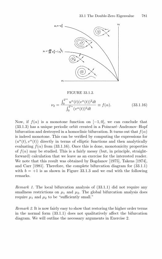
33.1 The Double-Zero Eigenvalue 781
FIGURE 33.1.2.
ν2 =
∫ T α
0 uα(t)(vα(t))2dt∫ T α
0 (vα(t))2dt≡ f(α). (33.1.16)
Now, if f(α) is a monotone function on [−1, 0], we can conclude that(33.1.3) has a unique periodic orbit created in a Poincare–Andronov–Hopfbifurcation and destroyed in a homoclinic bifurcation. It turns out that f(α)is indeed monotone. This can be verified by computing the expressions for(uα(t), vα(t)) directly in terms of elliptic functions and then analyticallyevaluating f(α) from (33.1.16). Once this is done, monotonicity propertiesof f(α) may be studied. This is a fairly messy (but, in principle, straight-forward) calculation that we leave as an exercise for the interested reader.We note that this result was obtained by Bogdanov [1975], Takens [1974],and Carr [1981]. Therefore, the complete bifurcation diagram for (33.1.1)with b = +1 is as shown in Figure 33.1.3 and we end with the followingremarks.
Remark 1. The local bifurcation analysis of (33.1.1) did not require anysmallness restrictions on µ1 and µ2. The global bifurcation analysis doesrequire µ1 and µ2 to be “sufficiently small.”
Remark 2. It is now fairly easy to show that restoring the higher order termsin the normal form (33.1.1) does not qualitatively affect the bifurcationdiagram. We will outline the necessary arguments in Exercise 2.
782 33. Global Bifurcations
FIGURE 33.1.3.
33.2 A Zero and a Pure Imaginary Pair ofEigenvalues
The normal form associated with this bifurcation is three-dimensional.However, the symmetry in the linear part associated with the pure imag-inary eigenvalues enabled us to decouple one of the coordinates from theremaining two so that we could begin our analysis using phase plane tech-niques. In some sense, the dynamics in this phase plane can be viewed asan approximation to a Poincare map of the full three-dimensional normalform. This is also a result of the symmetry of the linear part. Our analysiswill proceed in the following steps.
Step 1. Analyze global bifurcations of the associate truncated, two-dimen-sional normal form.
Step 2. Interpret in terms of the truncated, three-dimensional normal form.
Step 3. Discuss the effects of higher order terms in the normal form.
Step 1. Recall from Section 20.7 that the associated two-dimensional normalform of interest is given by
r = µ1r + arz,
z = µ2 + br2 − z2, (33.2.1)
where a = 0 and b = ±1. There were essentially only four distinct cases tostudy, and only two admitted the possibility of global bifurcations (for r,z small). They were denoted by
33.2 A Zero and a Pure Imaginary Pair of Eigenvalues 783
Case IIa,b a < 0, b = +1,Case III a > 0, b = −1.
In Case IIa,b we are interested in the dynamics near the µ2-axis for µ2 < 0.In Case III we are interested in the dynamics near the µ2-axis for µ2 > 0.In both cases the normal form was integrable on the µ2-axis (with theappropriate sign of µ2); thus, we would expect higher order terms in thenormal form to drastically affect the dynamics in this parameter regime.Our strategy will be to include the cubic terms in the normal form and tointroduce a scaling of the variables so that we obtain a perturbed Hamilto-nian system. Then a Melnikov-type analysis can be used to determine thenumber of periodic orbits and possible homoclinic bifurcations.
From (20.4.44), restoring the cubic terms to (33.2.1) gives
r = µ1r + arz + (cr3 + dr2z),z = µ2 + br2 − z2 + (er2z + fz3). (33.2.2)
In Guckenheimer and Holmes [1983] it is shown that coordinate changescan be introduced so that all cubic terms except for z3 in (33.2.2) can beeliminated (see Exercise 3 where we outline this procedure). Hence, withoutloss of generality, we can analyze the following normal form
r = µ1r + arz,
z = µ2 + br2 − z2 + fz3. (33.2.3)
We next rescale the dependent variables and parameters as follows
r = εu, z = εv, µ1 = ε2ν1, µ2 = ε2ν2, (33.2.4)
and we rescale time as follows
t −→ εt,
so that (33.2.2) becomes
u = auv + εν1u,
v = ν2 + bu2 − v2 + εfv3. (33.2.5)
At ε = 0, the vector field has the first integral (for a = 1)
F (u, v) =a
2u2/a
[ν2 +
b
1 + au2 − v2
]. (33.2.6)
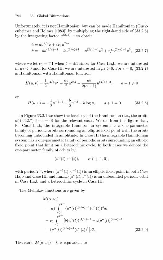
784 33. Global Bifurcations
Unfortunately, it is not Hamiltonian, but can be made Hamiltonian (Guck-enheimer and Holmes [1983]) by multiplying the right-hand side of (33.2.5)by the integrating factor u(2/a)−1 to obtain
u = au2/av + εν1u2/a,
v = −bu(2/a)−1 + bu(2/a)+1 − u(2/a)−1v2 + εfu(2/a)−1v3, (33.2.7)
where we let ν2 = ∓1 when b = ±1 since, for Case IIa,b, we are interestedin µ2 < 0 and, for Case III, we are interested in µ2 > 0. For ε = 0, (33.2.7)is Hamiltonian with Hamiltonian function
H(u, v) =12u2/av2 +
ab
2u2/a − ab
2(a + 1)u(2/a)+2, a + 1 = 0
orH(u, v) = −1
2u−2v2 − b
2u−2 − b log u, a + 1 = 0. (33.2.8)
In Figure 33.2.1 we show the level sets of the Hamiltonian (i.e., the orbitsof (33.2.7) for ε = 0) for the relevant cases. We see from this figure that,for Case IIa,b, the integrable Hamiltonian system has a one-parameterfamily of periodic orbits surrounding an elliptic fixed point with the orbitsbecoming unbounded in amplitude. In Case III the integrable Hamiltoniansystem has a one-parameter family of periodic orbits surrounding an ellipticfixed point that limit on a heteroclinic cycle. In both cases we denote theone-parameter family of orbits by
(uα(t), vα(t)), α ∈ [−1, 0),
with period Tα, where (u−1(t), v−1(t)) is an elliptic fixed point in both CaseIIa,b and Case III, and limα→0(uα(t), vα(t)) is an unbounded periodic orbitin Case IIa,b and a heteroclinic cycle in Case III.
The Melnikov functions are given by
M(α; ν1)
= af
∫ T α
0(uα(t))(4/a)−1(vα(t))4dt
− ν1
∫ T α
0
[b(uα(t))(4/a)+1 − b(uα(t))(4/a)−1
+ (uα(t))(4/a)−1(vα(t))2]dt. (33.2.9)
Therefore, M(α; ν1) = 0 is equivalent to
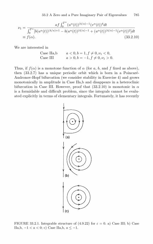
33.2 A Zero and a Pure Imaginary Pair of Eigenvalues 785
ν1 =af
∫ T α
0 (uα(t))(4/a)−1(vα(t))4dt∫ T α
0 [b(uα(t))(4/a)+1 − b(uα(t))(4/a)−1 + (uα(t))(4/a)−1(vα(t))2]dt
≡ f(α). (33.2.10)
We are interested inCase IIa,b a < 0, b = 1, f = 0, ν1 < 0,Case III a > 0, b = −1, f = 0, ν1 > 0.
Thus, if f(α) is a monotone function of α (for a, b, and f fixed as above),then (33.2.7) has a unique periodic orbit which is born in a Poincare-Andronov-Hopf bifurcation (we consider stability in Exercise 4) and growsmonotonically in amplitude in Case IIa,b and disappears in a heteroclinicbifurcation in Case III. However, proof that (33.2.10) is monotonic in αis a formidable and difficult problem, since the integrals cannot be evalu-ated explicitly in terms of elementary integrals. Fortunately, it has recently
FIGURE 33.2.1. Integrable structure of (4.9.22) for ε = 0. a) Case III; b) Case
IIa,b, −1 < a < 0; c) Case IIa,b, a ≤ −1.
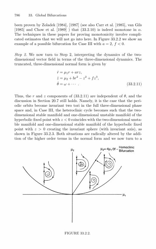
786 33. Global Bifurcations
been proven by Zoladek [1984], [1987] (see also Carr et al. [1985], van Gils[1985] and Chow et al. [1989] ) that (33.2.10) is indeed monotone in α.The techniques in these papers for proving monotonicity involve compli-cated estimates that we will not go into here. In Figure 33.2.2 we show anexample of a possible bifurcation for Case III with a = 2, f < 0.
Step 2. We now turn to Step 2, interpreting the dynamics of the two-dimensional vector field in terms of the three-dimensional dynamics. Thetruncated, three-dimensional normal form is given by
r = µ1r + arz,
z = µ2 + br2 − z2 + fz3,
θ = ω + · · · . (33.2.11)
Thus, the r and z components of (33.2.11) are independent of θ, and thediscussion in Section 20.7 still holds. Namely, it is the case that the peri-odic orbits become invariant two tori in the full three-dimensional phasespace and, in Case III, the heteroclinic cycle becomes such that the two-dimensional stable manifold and one-dimensional unstable manifold of thehyperbolic fixed point with z < 0 coincides with the two-dimensional unsta-ble manifold and one-dimensional stable manifold of the hyperbolic fixedpoint with z > 0 creating the invariant sphere (with invariant axis), asshown in Figure 33.2.3. Both situations are radically altered by the addi-tion of the higher order terms in the normal form and we now turn to a
FIGURE 33.2.2.
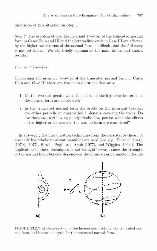
33.2 A Zero and a Pure Imaginary Pair of Eigenvalues 787
discussion of this situation in Step 3.
Step 3. The problem of how the invariant two-tori of the truncated normalform in Cases IIa,b and III and the heteroclinic cycle in Case III are affectedby the higher order terms of the normal form is difficult, and the full storyis not yet known. We will briefly summarize the main issues and knownresults.
Invariant Two-Tori
Concerning the invariant two-tori of the truncated normal form in CasesIIa,b and Case III there are two main questions that arise.
1. Do the two-tori persist when the effects of the higher order terms ofthe normal form are considered?
2. In the truncated normal form the orbits on the invariant two-toriare either periodic or quasiperiodic, densely covering the torus. Doinvariant two-tori having quasiperiodic flow persist when the effectsof the higher order terms of the normal form are considered?
In answering the first question techniques from the persistence theory ofnormally hyperbolic invariant manifolds are used (see, e.g., Fenichel [1971],[1979], [1977], Hirsch, Pugh, and Shub [1977], and Wiggins [1994]). Theapplication of these techniques is not straightforward, since the strengthof the normal hyperbolicity depends on the bifurcation parameter. Results
FIGURE 33.2.3. a) Cross-section of the heteroclinic cycle for the truncated nor-
mal form. b) Heteroclinic cycle for the truncated normal form.
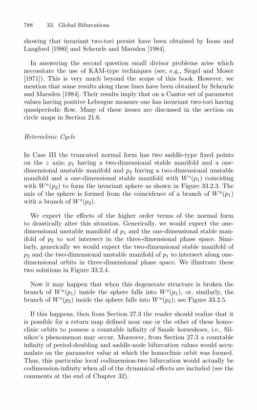
788 33. Global Bifurcations
showing that invariant two-tori persist have been obtained by Iooss andLangford [1980] and Scheurle and Marsden [1984].
In answering the second question small divisor problems arise whichnecessitate the use of KAM-type techniques (see, e.g., Siegel and Moser[1971]). This is very much beyond the scope of this book. However, wemention that some results along these lines have been obtained by Scheurleand Marsden [1984]. Their results imply that on a Cantor set of parametervalues having positive Lebesgue measure one has invariant two-tori havingquasiperiodic flow. Many of these issues are discussed in the section oncircle maps in Section 21.6.
Heteroclinic Cycle
In Case III the truncated normal form has two saddle-type fixed pointson the z axis; p1 having a two-dimensional stable manifold and a one-dimensional unstable manifold and p2 having a two-dimensional unstablemanifold and a one-dimensional stable manifold with W s(p1) coincidingwith Wu(p2) to form the invariant sphere as shown in Figure 33.2.3. Theaxis of the sphere is formed from the coincidence of a branch of Wu(p1)with a branch of W s(p2).
We expect the effects of the higher order terms of the normal formto drastically alter this situation. Generically, we would expect the one-dimensional unstable manifold of p1 and the one-dimensional stable man-ifold of p2 to not intersect in the three-dimensional phase space. Simi-larly, generically we would expect the two-dimensional stable manifold ofp2 and the two-dimensional unstable manifold of p1 to intersect along one-dimensional orbits in three-dimensional phase space. We illustrate thesetwo solutions in Figure 33.2.4.
Now it may happen that when this degenerate structure is broken thebranch of Wu(p1) inside the sphere falls into W s(p1), or, similarly, thebranch of W s(p2) inside the sphere falls into Wu(p2); see Figure 33.2.5.
If this happens, then from Section 27.3 the reader should realize that itis possible for a return map defined near one or the other of these homo-clinic orbits to possess a countable infinity of Smale horseshoes, i.e., Sil-nikov’s phenomenon may occur. Moreover, from Section 27.3 a countableinfinity of period-doubling and saddle-node bifurcation values would accu-mulate on the parameter value at which the homoclinic orbit was formed.Thus, this particular local codimension-two bifurcation would actually becodimension-infinity when all of the dynamical effects are included (see thecomments at the end of Chapter 32).
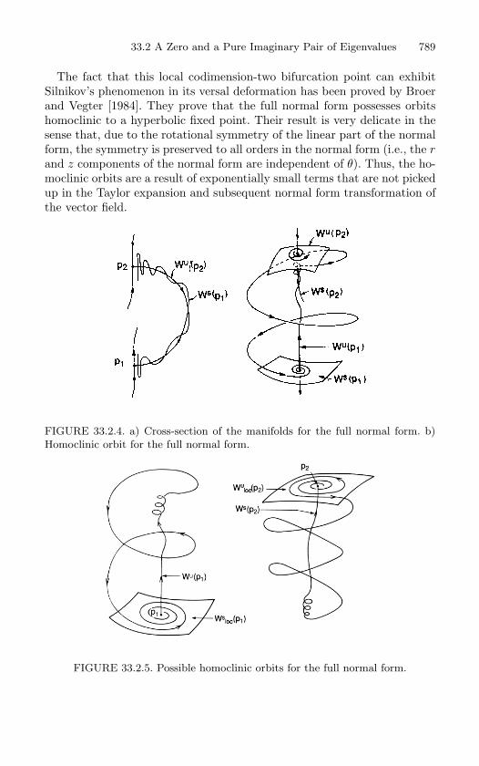
33.2 A Zero and a Pure Imaginary Pair of Eigenvalues 789
The fact that this local codimension-two bifurcation point can exhibitSilnikov’s phenomenon in its versal deformation has been proved by Broerand Vegter [1984]. They prove that the full normal form possesses orbitshomoclinic to a hyperbolic fixed point. Their result is very delicate in thesense that, due to the rotational symmetry of the linear part of the normalform, the symmetry is preserved to all orders in the normal form (i.e., the rand z components of the normal form are independent of θ). Thus, the ho-moclinic orbits are a result of exponentially small terms that are not pickedup in the Taylor expansion and subsequent normal form transformation ofthe vector field.
FIGURE 33.2.4. a) Cross-section of the manifolds for the full normal form. b)
Homoclinic orbit for the full normal form.
FIGURE 33.2.5. Possible homoclinic orbits for the full normal form.
790 33. Global Bifurcations
The Hamiltonian-Dissipative Decomposition
The key aspect that enabled the preceeding analyses to go through wasthe fact that one could find an “inspired” rescaling that transformed thenormal form into a perturbation of an integrable Hamiltonian system withthe higher order terms in the normal form part of the perturbation (note:the perturbation need not also be Hamiltonian). Once this has been ac-complished, a wealth of techniques for the global analysis of nonlinear dy-namical systems can then be employed; for example, Melnikov theory, per-turbation theory for normally hyperbolic invariant manifolds, and KAMtheory. However, the real question is, “in a given problem, how can we findthe rescalings which turn the problem into a perturbation of a completelyintegrable Hamiltonian system?”
The rescalings in this section are due to the cleverness of Takens [1974],Bogdanov [1975], Guckenheimer and Holmes [1983], Kopell and Howard[1975], and Iooss and Langford [1980]. However, in recent years there hasbeen an effort to understand the structure of the normal form that leads toa splitting of the normal form into a Hamiltonian part and a dissipative partso that the appropriate rescalings can be generated by some computationalprocedure. We refer the reader to Lewis and Marsden [1989] and Olver andShakiban [1988].
33.3 Exercises
1. Show that the function f(α) defined in (33.1.16) is monotone.
2. Show that the two-parameter family
x = y,
y = µ1 + µ2y + x2 + bxy, b = ±1, (33.3.1)
is a versal deformation of a fixed point of a planar vector field at which the matrixassociated with the linearization has the form
(0 10 0
).
(Hint: the idea is to show that the neglected higher order terms in the normal formdo not introduce any qualitatively new dynamics in the sense that the bifurcationdiagram in Figure 33.1.3 is unchanged. Begin by considering the fixed points and localbifurcations and show that these are qualitatively unchanged. Next, consider the globalbehavior, i.e., homoclinic orbits and “large amplitude” periodic orbits. The Melnikovtheory can be used here.
Once all of these results are established, does it then follow that (33.3.1) is a versaldeformation?)
3. Recall Exercise 1 following Section 20.6, the double-zero eigenvalue with the symmetry(x, y) → (−x, −y). The normal form was given by
33.3 Exercises 791
x = y,
y = µ1x + µ2y + cx3 − x
2y, c = ±1. (33.3.2)
In this exercise we want to analyze possible global behavior that might occur.
a) For c = +1, using the rescaling
x = εu, y = ε2v, µ1 = −ε
2, µ2 = ε
2ν2
and t → tε , show that (33.3.2) becomes
u = v,
v = −u + u3 + ε(ν2v − u
2v). (33.3.3)
b) Show that (33.3.3) is Hamiltonian for ε = 0 and draw the phase portrait.
c) Use the Melnikov theory to show that (33.3.3) has a heteroclinic connection on
µ2 = − µ1
5+ · · · . (33.3.4)
What is the form of the higher order terms in (33.3.4) (i.e., O(µα1 ), where α is
some number)? This is important for determining the behavior of the bifurcationcurves at the origin.
d) Show that (33.3.3) has a unique periodic orbit for µ1 < 0 between µ2 = 0 andµ2 = − µ1
5 + · · · .e) Draw the complete bifurcation diagram for (33.3.2) with c = +1. Is (33.3.2) a
versal deformation for c = +1?
f) For c = −1, using the rescaling
x = εu, y = ε2v, µ1 = ε
2, µ2 = ε
2ν2,
and t → tε , show that (33.3.2) becomes
u = v,
v = u − u3 + ε(ν2v − u
2v). (33.3.5)
g) Show that (33.3.5) is Hamiltonian for ε = 0 and draw the phase portrait.
h) Using the Melnikov theory, show that (33.3.5) undergoes a homoclinic bifurca-tion on
µ2 =45
µ1 + · · · , (33.3.6)
and a saddle-node bifurcation of periodic orbits on
µ2 = cµ1 + · · · , (33.3.7)
with c ≈ .752. Hence, for µ1 > 0, between µ2 = µ1 and µ2 = 45 µ1 + · · · ,
(33.3.2) has three periodic orbits for c = −1. What are their stabilities? Betweenµ2 = 4
5 µ1 + · · · and µ2 = cµ1 + · · · (33.3.2) has two periodic orbits for c = −1.What are their stabilities? Below µ2 = cµ1 + · · · there are no periodic orbits forc = −1.In (33.3.6) and(33.3.7) what is the form of the higher order terms (i.e., O(µα
1 )where α is some number).
1. Draw the complete bifurcation diagram for (33.3.2) with c = −1. Is (33.3.2)a versal deformation for c = −1?
(Hint: the Melnikov theory for autonomous systems is developed in Exercise 11 and theMelnikov theory for heteroclinic orbits is developed in Exercise 16 following Chapter28.)
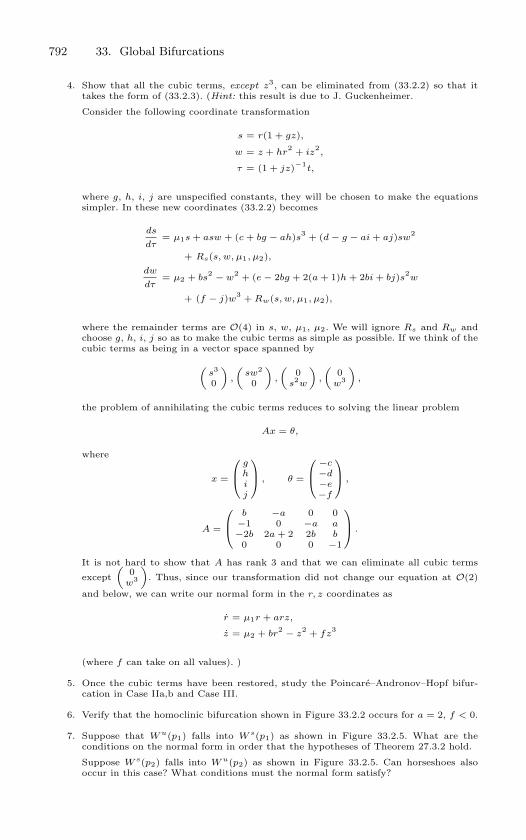
792 33. Global Bifurcations
4. Show that all the cubic terms, except z3, can be eliminated from (33.2.2) so that ittakes the form of (33.2.3). (Hint: this result is due to J. Guckenheimer.
Consider the following coordinate transformation
s = r(1 + gz),
w = z + hr2 + iz
2,
τ = (1 + jz)−1t,
where g, h, i, j are unspecified constants, they will be chosen to make the equationssimpler. In these new coordinates (33.2.2) becomes
ds
dτ= µ1s + asw + (c + bg − ah)s3 + (d − g − ai + aj)sw
2
+ Rs(s, w, µ1, µ2),dw
dτ= µ2 + bs
2 − w2 + (e − 2bg + 2(a + 1)h + 2bi + bj)s2
w
+ (f − j)w3 + Rw(s, w, µ1, µ2),
where the remainder terms are O(4) in s, w, µ1, µ2. We will ignore Rs and Rw andchoose g, h, i, j so as to make the cubic terms as simple as possible. If we think of thecubic terms as being in a vector space spanned by
(s3
0
),
(sw2
0
),
(0
s2w
),
(0
w3
),
the problem of annihilating the cubic terms reduces to solving the linear problem
Ax = θ,
where
x =
ghij
, θ =
−c−d−e−f
,
A =
b −a 0 0−1 0 −a a−2b 2a + 2 2b b0 0 0 −1
.
It is not hard to show that A has rank 3 and that we can eliminate all cubic terms
except(
0w3
). Thus, since our transformation did not change our equation at O(2)
and below, we can write our normal form in the r, z coordinates as
r = µ1r + arz,
z = µ2 + br2 − z
2 + fz3
(where f can take on all values). )
5. Once the cubic terms have been restored, study the Poincare–Andronov–Hopf bifur-cation in Case IIa,b and Case III.
6. Verify that the homoclinic bifurcation shown in Figure 33.2.2 occurs for a = 2, f < 0.
7. Suppose that W u(p1) falls into W s(p1) as shown in Figure 33.2.5. What are theconditions on the normal form in order that the hypotheses of Theorem 27.3.2 hold.
Suppose W s(p2) falls into W u(p2) as shown in Figure 33.2.5. Can horseshoes alsooccur in this case? What conditions must the normal form satisfy?
34
Glossary of Frequently UsedTerms
Absorbing set: A positive invariant compact subset B ⊂ Rn is called an absorbing set if
there exists a bounded subset of Rn, U , with U ⊃ B, and:
flows: tU > 0 such that φ(t, U) ⊂ B, ∀t ≥ tU .
maps: nU > 0 such that gn(U) ⊂ B, ∀n ≥ nU .
Action: The functional ∫ t1
t0
L(q1, . . . , qN , q1, . . . , qN , t)dt,
defined on curves in configuration space (such that the endpoints of each curve are fixed)and where L is the Lagrangian, is referred to as the action.
Action-Angle Coordinates, or Variables: These coordinates can be constructed for com-pletely integrable Hamiltonian systems that satisfy the hypotheses of the Liouville-Arnoldtheorem, and they are denoted by (θ, I), θ ∈ T n, I ∈ R
n. In these coordinates the Hamil-tonian is a function of only the action variable, I, i.e., H = H(I), and Hamilton’s equationsbecome:
θ =∂H
∂I,
I = − ∂H
∂θ= 0.
These equations can be easily integrated to yield the trajectories:
θ(t) =∂H
∂I(I0)t + θ(0),
I(t) = I0 = constant.
Hence, these are the trajectories on the n dimensional tori described by the Liouville-Arnold theorem. ∂H
∂I (I0) is referred to as the frequency of the torus I = I0.
Asymptotically Autonomous Vector Field: A vector field x = f(x, t), x ∈ Rn, is said to
be asymptotically autonomous if limt→∞ f(x, t) = g(x) exists.
Asymptotic Stability: Roughly, a trajectory is said to be asymptotically stable if it isLiapunov stable and, at a given time, trajectories starting close enough to the specifiedtrajectory approach the trajectory as time increases.
Attracting Set: Let φ(t, x) denote the flow generated by a vector field and let x → g(x)denote a map. A closed invariant set A ⊂ R
n is called an attracting set if there is someneighborhood U of A such that:
flows: ∀t ≥ 0, φ(t, U) ⊂ U and⋂
t>0 φ(t, U) = A.
maps: ∀n ≥ 0, gn(U) ⊂ U and⋂
n>0 gn(U) = A.
794 34. Glossary of Frequently Used Terms
Attractor: An attractor is a topologically transitive attracting set.
Autonomous System: A dynamical system that does not depend explicitly on the indepen-dent variable (which is often referred to as “time”).
Basin of Attraction: Let φ(t, x) denote the flow generated by a vector field and let x → g(x)denote a map. The domain or basin of attraction of an attracting set A is given by
flows:⋃t≤0
φ(t, U),
maps:⋃
n≤0
gn(U),
where U is any trapping region.
Bifurcation of a Fixed Point: A fixed point (x, µ) = (0, 0) of a one-parameter familyof one-dimensional vector fields, x = f(x, µ), or maps, x → f(x, µ), is said to undergoa bifurcation at µ = 0 if the flow for µ near zero and x near zero is not qualitativelythe same as the flow near x = 0 at µ = 0. A necessary, but not sufficient, condition forbifurcation of a fixed point is that the fixed point is non-hyperbolic.
Cantor Set: A compact, totally disconnected, perfect set.
Center Manifold of a Fixed Point: The center manifold of a fixed point is an invariantmanifold passing through a fixed point which is tangent to the center subspace at thefixed point, and has the same dimension as the center subspace.
Center Subspace of a Fixed Point: Consider an (autonomous) ordinary differential equa-tion (resp. map) linearized about a fixed point, and the Jacobian matrix associated withthis linearization. The center subspace associated with the fixed point is the span of thegeneralized eigenvectors corresponding to eigenvalues of the Jacobian matrix having zeroreal part (resp. modulus one). It is an invariant manifold under the linearized dynamics.
Chaotic Invariant Set: A compact set Λ invariant under a flow φ(t, x) (or map g(x)) is saidto be chaotic if
1. φ(t, x) (resp. g(x)) has sensitive dependence on initial conditions on Λ.
2. φ(t, x) (resp. g(x)) is topologically transitive on Λ.
Cocycle: Let P denote a parameter space. Let Θ = θt | t ∈ R denote a one-parameterfamily of mappings of P into itself, i.e.,
θt : P → P,
p → θtp,
withθt θs = θt+s, ∀t, s ∈ R,
andθ0 = id.
Then a family of mappings
φt,p : Rn → R
n, t ∈ R, p ∈ P,
is called a cocycle on Rn with respect to a group Θ of mappings on P if:
1. φ0,p = id,
2. φt+s,p = φt,θsp φs,p,
34. Glossary of Frequently Used Terms 795
for all t, s ∈ R, p ∈ P .
Codimension of a Submanifold: Let M be an m-dimensional manifold and let N be ann-dimensional submanifold contained in M ; then the codimension of N is defined to bem − n. Equivalently, in a coordinate setting, the codimension of N is the number ofindependent equations needed to define N . Thus, the codimension of a submanifold is ameasure of the avoidability of the submanifold as one moves about the ambient space; inparticular, the codimension of a submanifold N is equal to the minimum dimension of asubmanifold P ⊂ M that intersects N such that the intersection is transversal. This isthe definition of codimension in a finite-dimensional setting, which permits some intuitionto be gained; now we move to the infinite-dimensional setting. Let M be an infinite-dimensional manifold and let N be a submanifold contained in M . Roughly speaking,an infinite-dimensional manifold is a set which is locally diffeomorphic to an infinite-dimensional Banach space. Because infinite-dimensional manifolds are discussed in thissection only, and then mainly in a heuristic fashion, we refer the reader to the literaturefor the proper definitions.) We say that N is of codimension k if every point of N iscontained in some open set in M which is diffeomorphic to U × R
k, where U is an openset in N . This implies that k is the smallest dimension of a submanifold P ⊂ M thatintersects N such that the intersection is transversal. Thus, the definition of codimensionin the infinite-dimensional case has the same geometrical connotations as in the finite-dimensional case. Now we return to our main discussion. (For the case of “codimension∞”, R
k in this definition is replaced with an infinite dimensional Banach space.)
Completely Integrable Hamiltonian System: Hamilton’s equations, for n degrees-of-freedom, are said to be completely integrable if there exists n functions (called integrals)
F1 ≡ H, F2, · · · , Fn, (H is the Hamiltonian),
which satisfy the following conditions.
1. The Fi, i = 1, · · · , n, are functionally independent on U , with the possible exceptionof sets of measure zero.
2. Fi, Fj = 0, for all i and j, where ·, · denotes the Poisson bracket.
Configuration Space: The space of generalized coordinates of a system is often referred toas the configuration space of the system.
Conjugacy: A change of variables, or coordinates. Consider two Cr diffeomorphisms f : Rn →
Rn and g: R
n → Rn, and a Ck diffeomorphism h: R
n → Rn. f and g are said to be Ck
conjugate (k ≤ r) if there exists a Ck diffeomorphism h: Rn → R
n such that g h = h f .If k = 0, f and g are said to be topologically conjugate.
The conjugacy of two diffeomorphisms is often represented by the following diagram.
Rn f−→ R
n'h
'h
Rn g−→ R
n
.
The diagram is said to commute if the relation g h = h f holds, meaning that you canstart at a point in the upper left-hand corner of the diagram and reach the same point inthe lower right-hand corner of the diagram by either of the two possible routes. We notethat h need not be defined on all of R
n but possibly only locally about a given point. Insuch cases, f and g are said to be locally Ck conjugate.
Conley-Moser Conditions: A set of geometrical and analytical criteria for a map that, ifsatisfied, imply that the map behaves like a Smale horseshoe.
Cr Function: A function is said to be Cr if it is r times differentiable, and if each of thederiviatives is a continuous function. For r = 0 the function is merely continuous.
Cr Diffeomorphism: A function is said to be a Cr diffeomorphism if the function is invert-ible, and if both the function and its inverse are Cr functions. For r = 0 the function issaid to be a homeomorphism.
Cyclic Coordinate: A synonym for ignorable coordinate.
Degrees of Freedom: The phrase degrees of freedom has its origins in mechanics. The num-ber of degrees of freedom of a mechanical system is the number of independent coordinates
796 34. Glossary of Frequently Used Terms
that are required to describe the configuration of the system (i. e., “position coordinates”).Thus, the number of degrees of freedom is half the dimension of the phase space of thecorresponding Hamiltonian dynamical system. If an n degree of freedom system also de-pends explicitly on time (i.e., the vector field is nonautonomous), the the phrase n + 1
2degree of freedom system is often used.
Diophantine Frequency: A frequency vector ω ∈ Rn is said to be diophantine if there
exists constants τ, γ > 0 such that the following infinite number of inequalities hold:
|ω · k| ≥ γ|k|−τ ∀k ∈ ZZn − 0
where|k| ≡ sup
i|ki|.
Distance Between a Point and a Set: Let S ∈ Rn be an arbitrary set and p ∈ R
n bean arbitrary point. Then the distance between the point p and the set S is denoted anddefined as:
d(p, S) = infx∈S
|p − x|. (34.0.1)
Double-Hopf Bifurcation: The bifurcation associated with a nonhyperbolic equilibriumpoint of an autonomous vector field where the matrix associated with the linearization ofthe the vector field about the equilibrium point has the following Jordan canonical form:
0 ω1 0 0ω1 0 0 00 0 0 −ω20 0 ω2 0
.
Duffing Equation: The second order, ordinary differential equation:
x − x + x3 = 0, x ∈ R,
or, written as a system
x = y,
y = x − x3, (x, y) ∈ R
2.
Sometimes damping and external driving (time-dependence) are added
x = y,
y = x − x3 − δy + γf(t), (x, y) ∈ R
2,
in this case it is referred to as the damped (δy), driven (γf(t)) Duffing equation, where δand γ are parameters.
Dynamical System: A system that changes in time; usually described by differential equa-tions (continuous time) or difference equations (sometimes called “maps) (discrete time),or, possibly, some combination of the two.
Elliptic Equilibrium Point: An equilibrium point of an autonomous Hamiltonian system issaid to be elliptic if all of the eigenvalues of the matrix associated with the linearizationabout the equilibrium point are purely imaginary, and nonzero.
Equilibrium Solution: A constant solution of a vector field, i.e. a point in phase spacewhere the vector field is zero, also referred to as a fixed point.
Exponential Dichotomy: The linear field x = A(t)x, x ∈ Rn is said to possess an exponen-
tial dichotomy if each of the n linear independent solutions exhibit exponential growthor decay as t → ∞. More precisely, suppose X(t) is the fundamental solution matrix ofthis linear vector field, i.e., for any initial condition ξ0, ξ(t) = X(t)ξ0 is the solution ofthe vector field passing through ξ0 at t = 0, X(0) = id. Let ‖ · ‖ denote a norm on R
n.Then the linear vector field is said to possess an exponential dichotomy if there exists aprojection operator P , P 2 = P , and constants K1, K2, λ1, λ2 > 0, such that
34. Glossary of Frequently Used Terms 797
‖ X(t)PX−1(τ) ‖ ≤ K1 exp (−λ1(t − τ)) , t ≥ τ,
‖ X(t) (id − P ) X−1(τ) ‖ ≤ K2 exp (λ2(t − τ)) , t ≤ τ.
Extended Phase Space: The cartesian product of the phase space with the independentvariable (which is often referred to as “time”).
Fold Bifurcation: Another term for a saddle-node bifurcation.
Γ-Equivariant Map: Let f : V → V denote a mapping of a vector space V into V . Let Γdenote a compact Lie group with a specified action on V . We say that f is Γ-equivariantwith respect to this action if
f(γx) = γf(x), ∀γ ∈ Γ, x ∈ V.
Γ-Invariant Function: Now let f : V → R denote a mapping of a vector space V into R. LetΓ denote a compact Lie group with a specified action on V . We say that f is Γ-invariantwith respect to this action if
f(γx) = f(x), ∀γ ∈ Γ, x ∈ V.
If f is a vector field then we will refer to it as a Γ- equivariant vector field. It follows that ifx(t) is a solution of a Γ-equivariant vector field x = f(x), then γx(t) is also a solution,for each γ ∈ Γ.
General Linear Group, GL(Rn): GL(Rn) is the group of linear, invertible transformationsof R
n into Rn, which we can view as the group of nonsingular n × n matrices over R.
Generalized Coordinates: A set of coordinates that contain the minimum number of in-dependent coordinates needed to specify all the positions of a set of particles is referredto as generalized coordinates, and denoted by (q1, . . . , qN ). Generalized coordinates maybe distances, angles, or quantities relating them. The integer N is referred to as the num-ber of degrees-of-freedom of a system. So a system is said to have N degrees-of-freedomif the positions of all its components can be described by N independent (generalized)coordinates.
Generalized Momentum: pi = ∂L∂qi
is referred to as the ith component of generalizedmomentum.
Generalized Velocity: (q1, . . . , qN ) are referred to as generalized velocities, where(q1, . . . , qN ) are generalized coordinates.
Generating Function: Consider the Hamiltonian
H(q, p, t),
and the associated Hamilton’s equations:
q =∂H
∂p(q, p, t),
p = − ∂H
∂q(q, p, t).
Suppose we have a transformation of coordinates of the form
Q = Q(q, p, t),
P = P (q, p, t),
which we assume can be inverted (viewing t as fixed) to yield
q = q(Q, P, t),
p = p(Q, P, t).
The Hamiltonian in the original (q, p) coordinates can be written as a function of the (Q, P )coordinates:
798 34. Glossary of Frequently Used Terms
H(q, p, t) = H(Q, P, t).
In the Q − P coordinates Hamilton’s equations will hold, i.e.,
Q =∂H
∂P(Q, P, t),
P = − ∂H
∂Q(Q, P, t).
provided the coordinate transformation satisfies:
pi =∂F
∂qi
,
Pi = − ∂F
∂Qi
,
H = H +∂F
∂t,
where the function F satisfies:
dF (q, Q, t) =N∑
i=1
pidqi −N∑
i=1
PidQi + (H − H)dt.
The function F is referred to as a generating function.
Generic Property: A property of a map (resp. vector field) is said to be Ck generic if theset of maps (resp. vector fields) possessing that property contains a residual subset in theCk topology.
Gradient Vector Field: A gradient vector field is a vector field having the form x =∇V (x), x ∈ R
n, where V (x) is a scalar valued function.
Group: A group is a set, G, equipped with a binary operation on the group elements, denoted“∗” and referred to as group multiplication, which satisfies the following three properties.
1. G is closed under group multiplication, i.e., g1, g2 ∈ G ⇒ g1 ∗ g2 ∈ G.
2. There exists a multiplicative identity element in G, i.e., there exists an elemente ∈ G such that e ∗ g = g ∗ g = g, for any g ∈ G.
3. For every element of G there exists a multiplicative inverse, i.e., for every g ∈ G,there exists an element, denoted g−1, such that g ∗ g−1 = g−1 ∗ g = e.
4. Multiplication is associative, i.e., (g1∗g2)∗g3 = g1∗(g2∗g3), for any g1, g2, g3 ∈ G.
Hamilton’s Equations: The ordinary differential equations:
qi =∂H
∂pi
,
pi = − ∂H
∂qi
, i = 1, . . . , N,
are referred to as Hamilton’s equations, where H = H(q, p) is a scalar valued functioncalled the Hamiltonian.
Hamilton-Jacobi Equation: The partial differential equation
∂S
∂t+ H
(q,
∂S
∂q, t
)= 0,
for some scalar valued function H (q ∈ RN ) is referred to as the Hamilton-Jacobi equation.
34. Glossary of Frequently Used Terms 799
Hausdorff Metric: Let A and B be two nonempty, compact subsets of Rn. The Hausdorff
metric defined on the set of nonempty, compact subsets of Rn is defined as:
H(A, B) ≡ max(H
∗(A, B), H∗(B, A)
).
Hausdorff Separation: Let A and B be two nonempty, compact subsets of Rn. The Haus-
dorff separation of A and B, denoted H∗(A, B), is defined as:
H∗(A, B) ≡ max
a∈Adist (a, B) = max
a∈Aminb∈B
‖ a − b ‖ .
Heteroclinic Orbit: An orbit is said to be heteroclinic to the two invariant sets Λ1 andΛ2 if it approaches Λ1 asymptotically under time evolution as time goes to −∞ andapproaches Λ2 asymptotically under time evolution as time goes to +∞. If the invariantsets have stable and unstable manifolds then a heteroclinic orbit lies in the intersectionof the unstable manifold of Λ1 and the stable manifold of Λ2.
Homoclinic Orbit: An orbit is said to be homoclinic to an invariant set if it approachesthe invariant set asymptotically under time evolution as time goes to ±∞. If the invariantset has stable and unstable manifolds then a homoclinic orbit lies in the intersection ofthe stable and unstable manifolds.
Hopf Bifurcation: See Poincare-Andronov-Hopf bifurcation.
Hopf-Steady State Bifurcation: The bifurcation associated with a nonhyperbolic equilib-rium point of an autonomous vector field where the matrix associated with the lineariza-tion of the the vector field about the equilibrium point has the following Jordan canonicalform:
0 −ω 0ω 0 00 0 0
.
Hyperbolic Fixed Point: A fixed point of a vector field that has the property that none ofthe eigenvalues of the matrix associated with the linearization of the vector field at thefixed point lie on the imaginary axis. A fixed point of a map or difference equation that hasthe property that none of the eigenvalues of the matrix associated with the linearizationof the map at the fixed point lie on the unit circle.
Hyperbolic Trajectory: The trajectory x(t) of the vector field x = f(x, t) is said to behyperbolic if the associated linear equation, ξ = Dxf(x(t), t)ξ, possesses and exponentialdichotomy.
Ignorable Coordinate: A generalized coordinate that does not appear in the Lagrangian(although the generalized velocity corresponding to the coordinate may appear in theLagrangian).
Index of a Closed Curve: Consider an autonomous vector field defined in some simplyconnected region, R, of the plane (this is a two-dimensional idea only). Let Γ be anyclosed loop in R which contains no fixed points of the vector field. You can imagine ateach point, p, on the loop Γ that there is an arrow representing the value of the vectorfield at p.
Now as you move around Γ in the counter-clockwise sense (call this the positive direction),the vectors on Γ rotate, and when you get back to the point at which you started, theywill have rotated through an angle 2πk, where k is some integer. This integer, k, is calledthe index of Γ.
The index of a closed curve containing no fixed points can be calculated by integrating thechange in the angle of the vectors at each point on Γ around Γ (this angle is measuredwith respect to some chosen coordinate system). For a vector field defined on some simplyconnected region, R, of the plane given by
x = f(x, y),
y = g(x, y), (x, y) ∈ R ⊂ R2,
the index of Γ, k, is found by computing
800 34. Glossary of Frequently Used Terms
k =12π
∮Γ
dφ =12π
∮Γ
d
(tan−1 g(x, y)
f(x, y)
)
=12π
∮Γ
f dg − g df
f2 + g2.
Infinitesimally Symplectic Transformations: Consider a Cr, r ≥ 1, map f : R2n → R
2n.Then f is said to be an infinitesimally symplectic or Ω skew transformation if
Ω(Df(x)u, v) = −Ω(u, Df(x)v), ∀x, u, v ∈ R2n
,
where Ω denotes a symplectic form on R2n. In terms of the canonical symplectic form this
relation takes the form:JDf(x) + Df(x)T
J = 0.
Infinitesimally symplectic maps arise in the study of the linearization of Hamiltonianvector fields at equilibria.
Infinitesimally Reversible Linear Map: Suppose G : Rn → R
n is a linear involution andA : R
n → Rn is a linear map. Then A is said to be infinitesimally reversible if
AG + GA = 0.
This linearization condition is defined at a symmetric fixed point. Infinitesimally reversiblelinear maps arise in the study of the linearization of reversible vector fields at symmetricfixed points.
Integral Curve: A trajectory in extended phase space.
Invariant Manifold: An invariant set, which is also a manifold.
Invariant Set: A set of points in phase space that has the property that trajectories withinitial conditions in the set remain in the set forever.
Involution: Consider a Cr mapG : R
n → Rn
,
satisfyingG G = id,
where id stands for the identity map. G is called an involution
Kolmogorov-Arnold-Moser (KAM) Theorem: This is a perturbation theorem that ap-plies to perturbations of completely integrable Hamiltonian systems expressed in action-angle coordinates. It states that for sufficiently small perturbations the tori in the un-perturbed, completely integrable system corresponding to diophantine frequency vectorpersist for the perturbed system.
Lagrangian: The scalar valued function L = T − V is referred to as the Lagrangian of asystems, where T is the kinetic energy and V is the potential energy.
Lagrange’s Equations: ddt
∂L∂qi
− ∂L∂qi
= 0, i = 1, . . . , N , are referred to as Lagrange’s equa-tions for an N degree-of-freedom system, where q1, . . . , qN are generalized coordinates,and L is the Lagrangian.
Liapunov Function: A scalar valued function, defined on the phase space (or, possibly justsome subset thereof) whose level sets define trapping regions for the trajectories of adynamical system.
Liapunov Stability: Roughly, a trajectory is said to be Liapunov stable if, at a given time,trajectories starting close enough to the specified trajectory remain close for all later time.
Lie Group: A Lie group is a closed subgroup of GL(Rn), which we will denote by Γ.
A subgroup is a subset of a group, which obeys the same axioms as a group (but with theimportant point that it is the subset that is closed with respect to group multiplication).The term “closed” in the definition of a Lie group needs clarification. We can identify thespace of all n × n matrices with Rn2
. Then GL(Rn) is an open subset of Rn2. Γ is said to
be a closed subgroup if it is a closed subset of GL(Rn), as well as a subgroup of GL(Rn).
34. Glossary of Frequently Used Terms 801
If this closed subset is compact or connected then the associated Lie group is also said tobe compact or connected.
Lie Group Action on a Vector Space: Let Γ denote a Lie group and V a vector space. Wesay that Γ acts linearly on V if there is a continuous mapping, referred to as the action:
Γ × V → V,
(γ, v) → γ · v,
such that
1. For each γ ∈ Γ the mapping
ργ : V → V,
v → γ · v ≡ ργ(v).
is linear.
2. (a) For any γ1, γ2 ∈ Γ,γ1 · (γ2 · v) = (γ1 ∗ γ2) · v.
(b) e · v = v.
The Lift of a Circle Map: Consider the following map of the real line R to S1:
Π : R −→ S1,
x −→ e2πix ≡ θ.
The map F : R −→ R is said to be a lift of f : S1 −→ S1 if
Π F = f Π.
Linearization: The procedure of Taylor expanding a dynamical system in the dependentvariable about a specific solution, or invariant set, and throwing away all but the termslinear in the dependent variable.
Liouville-Arnold Theorem: This theorem describes the phase space structure of certainn degree-of-freedom completely integrable Hamiltonian systems. Suppose F1, . . . , Fn aren integrals satisfying the definition of complete integrability. Then we examine the (ingeneral) n dimensional sets defined by
F1 = f1,
......
Fn = fn,
where the fi, i = 1, . . . , n are constants. The Liouville-Arnold theorem states that if thesesets are compact and connected, then they are actually n-tori.
Multiplicity of a Resonance: A resonant frequency vector ω ∈ Rn is said to be of multi-
plicity m < n if there exist independent ki ∈ ZZn − 0, i = 1, . . . , m, such that ki · ω = 0.
Naimark-Sacker Torus Bifurcation: A bifurcation of a fixed point of a map where thelinearization has a pair of eigenvalues on the unit circle. The eigenvalues satisfy a non-resonance condition in the sense that they are no one of the first four roots of unity, i.e.,if λ denotes one of the eigenvalues then λn = 1, n = 1, 2, 3, 4. The bifurcation of thefixed point gives rise to an invariant circle. This bifurcation is sometimes referred to asthe “Hopf bifurcation for maps”.
Negative Invariant Manifold: A negative invariant set that is also a manifold.
Negative Invariant Set: A set of points in phase space that has the property that trajec-tories with initial conditions in the set remain in the set for all negative time.
802 34. Glossary of Frequently Used Terms
Nekhoroshev’s Theorem: This is a perturbation theorem that applies to perturbations ofcompletely integrable Hamiltonian systems expressed in action-angle coordinates. It statesthat for sufficiently small perturbations the action variable change by a small amount overan exponentially long time interval.
Node: An equilibrium point of a vector field having the property that the matrix associatedwith the linearization at the fixed point has all eigenvalues either in the right or the lefthalf plane. Hence, a node is a hyperbolic fixed point that is either attracting or repelling.
Nonautonomous System: A dynamical system that depends explicitly on the independentvariable (which is often referred to as “time”).
Nonwandering Points: Let φ(t, x) denote the flow generated by a vector field and letx → g(x) denote a map. A point x0 is called nonwandering if the following holds.
Flows: For any neighborhood U of x0 and T > 0, there exists some |t| > T such that
φ(t, U) ∩ U = ∅.
Maps: For any neighborhood U of x0, there exists some n = 0 such that
gn(U) ∩ U = ∅.
Note that if the map is noninvertible, then we must take n > 0.
Nonwandering Set: The set of all nonwandering points of a map or flow is called thenonwandering set of that particular map or flow.
ω and α Limit Points of Trajectories: Let φ(t, x) denote the flow generated by a vectorfield. A point x0 ∈ R
n is called an ω limit point of x ∈ Rn, denoted ω(x), if there exists
a sequence ti, ti −→ ∞, such that
φ(ti, x) −→ x0.
α limit points are defined similarly by taking a sequence ti, ti −→ −∞.
ω and α Limit Sets of a Flow: The set of all ω limit points of a flow or map is called theω limit set. The α limit set is similarly defined.
Normal Form: A local theory that applies in the neighborhood of an orbit of a vectorfield or map. The theory provides an algorithmic way to generate a sequence of nonlinearcoordinate changes that eliminate as much of the nonlinearity as possible at each order(where “order” refers to the terms in a Taylor expansion about the orbit). Interestingly,the form of the nonlinearity that cannot be eliminated by such coordinate changes isdetermined by the structure of the linear part of the vector field or map.
Orbit: The set of points in phase space through which a trajectory passes.
Orbital Derivative: Consider a dynamical system, with its phase space, and a functiondefined on this phase space. The orbital derivative of the function is the derivative of thefunction along trajectories of this dynamical system.
Order of a Resonance: Suppose ω ∈ Rn is a frequency vector and k · ω = 0 for some
k ∈ ZZn − 0. Then the order of this resonance is defined to be |k| =∑
i
|ki|.
Perfect Set: A set is called perfect if it is closed and every point in the set is a limit pointof the set.
Period-Doubling Bifurcation: A bifurcation of a fixed point of a map where the lineariza-tion at the fixed point has an eigenvalue of −1. In this bifurcation the fixed point (i.e.,period one point) changes its stability type and a period two orbit is created (or destroyed).
Phase Curve: The solution of an ordinary differential equation, synonomous with the termtrajectory.
Phase Space: The space of dependent variables of an ordinary differential equation or map.
Poincare-Andronov-Hopf Bifurcation: A bifurcation of a fixed point of a vector fieldwhere the linearization has a pair of purely imaginary eigenvalues (which are not zero).Provided a nondegeneracy condition involving the quadratic and cubic nonlinear termsholds, this bifurcation gives rise to a unique periodic orbit.
34. Glossary of Frequently Used Terms 803
Poincare-Bendixson Theorem: A theorem that applies to two- dimensional, autonomousvector fields on the sphere, or on a compact, positively invariant subset of R
2. It statesthat the omega limit sets are either equilibrium points, periodic orbits, or a collection oforbits made up of fixed points and orbits connecting fixed points (heteroclinic orbits) thatform a closed path.
Poincare Map: A map obtained from the trajectories of an ordinary differential equation.There are many ways in which this can be done. However, a guiding principle is that thedynamics of the map must correspond to the dynamics of the vector field.
Poisson Bracket: Let H, G : U → R, U ⊂ R2n, denote two Cr, r ≥ 2, functions. Then the
Poisson bracket of these two functions is another function, and it is defined through thesymplectic form Ω on R
2n as follows:
H, G ≡ Ω(XH , XG) ≡ 〈XH , JXG〉,
where XH and XG denote the Hamiltonian vector fields corresponding to the Hamiltonianfunctions H and G, respectively.
Positive Invariant Manifold: A positive invariant set that is also a manifold.
Positive Invariant Set: A set of points in phase space that has the property that trajectorieswith initial conditions in the set remain in the set for all positive time.
Pullback Absorbing Family: A family
B = Bp, p ∈ P ,
of compact subsets of Rn is called a pullback absorbing family for a cocycle
φt,p, t ∈ R, p ∈ P on Rn if for each p ∈ P there is a bounded subset of R
n, Up, satisfyingUp ⊃ Bp, and a time tUp > 0 such that:
φt,θ−tp(Uθ−tp) ⊂ Bp, for all t ≥ tUp .
Pullback Attracting Set: A family A = Ap, p ∈ P of compact subsets of Rn is called
a pullback attracting set of a cocycle φt,p, t ∈ R, p ∈ P on Rn if it is invariant in the
sense that:φt,p (Ap) = Aθtp, t ∈ R, p ∈ P,
and pullback attracting in the sense that for every Ap there exists a bounded subset ofR
n, Dp ⊃ Ap, such that
limt→∞ H
∗ (φt,θ−tp(Dθ−tp), Ap
)= 0.
Principle of Least Action: The principle of least action states that extrema of the actionfunctional are solutions of Lagrange’s equations, and vice-versa.
Quasiperiodic Motion: A function
h : R1 → R
m
t → h(t)
is called quasiperiodic if it can be represented in the form
h(t) = H(ω1t, . . . , ωnt),
where H(x1, . . . , xn) is a function of period 2π in x1, . . . , xn. The real numbersω1, . . . , ωn are called the basic frequencies. We shall denote by Cr(ω1, . . . , ωn) theclass of h(t) for which H(x1, . . . , xn) is r times continuously differentiable.
For example, the functionh(t) = γ1 cos ω1t + γ2 sin ω2t
is a quasiperiodic function.
804 34. Glossary of Frequently Used Terms
(Note: There exists a more general class of functions called almost periodic functionswhich can be viewed as quasiperiodic functions having an infinite number of basic fre-quencies. These will not be considered in this book, see Hale [1980] for a discussion andrigorous definitions.)
A quasiperiodic solution φ(t), of an ordinary differential equation is a solution which isquasiperiodic in time. A quasiperiodic orbit is the orbit of any point through which φ(t)passes. A quasiperiodic orbit may be interpreted geometrically as lying on an n dimen-sional torus. This can be seen as follows. Consider the equation
y = H(x1, . . . , xn).
Then, if m ≥ n and DxH has rank n for all x = (x1, . . . , xn), then this equation can beviewed as an embedding of an n-torus in m space with x1, . . . , xn serving as coordinateson the torus. Now, viewing h(t) as a solution of an ordinary differential equation, sincexi = ωit, i = 1, . . . , n, h(t) can be viewed as tracing a curve on the n-torus as t varies.
Representation of Γ on V : Let GL(V ) denote the group of invertible linear transformationsof V into V . The map
ρ : Γ → GL(V ),
γ → ργ ,
is called a representation of Γ on V .
Resonance: The frequency vector ω ∈ Rn is said to be resonant if there exists k ∈ ZZn − 0
such that k · ω = 0. If no such k ∈ ZZn − 0 exists, ω is said to be nonresonant.
Residual Set: Let X be a topological space, and let U be a subset of X. U is called a residualset if it is the intersection of a countable number of sets each of which are open and densein X. If every residual set in X is itself dense in X, then X is called a Baire space.
Reversible Dynamical System: Let x = f(x), x ∈ Rn be a vector field and let G :
Rn → bbRn be an involution. Then the vector field is said to be reversible if d
dt (G(x)) =−f (G(x)). A map xn+1 = g(xn) is said to be reversible if g (G(xn+1)) = G(xn).
Reversible Linear Map: Suppose G : Rn → R
n is a linear involution and A : Rn → R
n isa linear map. Then A is said to be reversible if
AGA = G.
Note that this linearization condition is defined at a symmetric fixed point. Reversiblelinear maps arise in the study of the linearization of reversible maps at symmetric fixedpoints.
Rotation Number: Consider an orientation preserving homeomorphism f : S1 −→ S1, withF a lift of f , we define the quantity
ρ0(F ) ≡ limn→∞
|F n(x)|n
.
There are two main operational definitions of rotation number. For f : S1 −→ S1 anorientation preserving homeomorphism, with F a lift of f :
1. Some authors define the rotation number of f , denoted ρ(f), as the fractional partof ρ0(F ) (e.g. Devaney [1986]).
2. Other authors define the rotation number of f to be ρ0(F ) (e.g., Katok and Has-selblatt [1995]).
In either case, the rotation number exists, and is independent of the point x.
Saddle-Node Bifurcation: A bifurcation of a fixed point where one goes from zero to twofixed points as a parameter is varied through the bifurcation point. At the bifurcationpoint the linearization has a zero eigenvalue for vector fields and an eigenvalue of one formaps. This bifurcation is also referred to as a tangent or fold bifurcation.
Sensitive dependence on initial conditions: Consider Cr (r ≥ 1) autonomous vectorfields and maps on R
n denoted as follows
34. Glossary of Frequently Used Terms 805
vector field x = f(x), (34.0.2)
map x → g(x). (34.0.3)
Denote the flow generated by (34.0.2) by φ(t, x) and we assume that it exists for allt > 0. We assume that Λ ⊂ R
n is a compact set invariant under φ(t, x) (resp. g(x)), i.e.,φ(t, Λ) ⊂ Λ for all t ∈ R (resp. gn(Λ) ⊂ Λ for all n ∈ Z, except that if g is not invertible,we must take n ≥ 0). The flow φ(t, x) (resp. g(x)) is said to have sensitive dependence oninitial conditions on Λ if there exists ε > 0 such that, for any x ∈ Λ and any neighborhoodU of x, there exists y ∈ U and t > 0 (resp. n > 0) such that |φ(t, x) − φ(t, y)| > ε (resp.|gn(x) − gn(y)| > ε).
Shift Map: A map defined on the space of bi-infinite sequences of N symbols (see symbolsequence). It acts by shifting the sequence one place to the left of the point separatingthe sequence into two infinite halves. More precisely, if we denote the shift map by σ, anda symbol sequence by
s =
· · · s−n · · · s−1.s0s1 · · · sn · · ·
where si ∈ 1, 2, . . . , N ∀ i.
Thenσ(
· · · s−n · · · s−1.s0s1 · · · sn · · ·)
=
· · · s−n · · · s−1s0.s1 · · · sn · · ·
.
Skew-Product Flow: This is a formalism that can be applied to nonautonomous vectorfields which allows one to retain the flow property. The crucial observation leading to thedevelopment of the approach is the following. Suppose x(t) is a solution of x = f(x, t).Then xτ (t) ≡ x(t + τ) is a solution of xτ (t) = fτ (xτ (t), t) ≡ f(x(t + τ), t + τ)
We first define the space of nonautonomous vector fields whose time translates remain withinthe space, i.e.,
F ≡ Space of functions f : Rn × R → R
n such thatfτ (·, ·) ≡ f(·, · + τ) ∈ F for all τ ∈ R.
We then define the group of shift operators on F :
θτ : F → F,
f → θτ f ≡ fτ , ∀τ ∈ R,
and we define the product space:X ≡ R
n × F.
Let x(t, x0, f) denote a solution of x = f(x, t) with x(0, x0, f) = x0. Finally, we definethe family of mappings:
Ψt : X → X ,
(x0, f) → (x(t, x0, f), θtf) .
It can then be shown that Ψt is a one-parameter family of mappings of X into X , or flow:
Ψt+s(x0, f) = Ψt Ψs(x0, f).
Smale Horseshoe: As originally conceived by Smale, a two-dimensional, nonlinear, invertiblemap possessing an invariant set with a remarkable structure. The invariant set has thestructure of a Cantor set. In addition, it has a countable infinity of periodic orbits of allpossible periods, an uncountable infinity of nonperiodic orbits, and an orbit that is densein the invariant set. The dynamics on the invariant set is chaotic. The map has since been
806 34. Glossary of Frequently Used Terms
generalized to many other settings (n dimensions as well as infinite dimensions, and inalso in the context of noninvertible maps).
Space of Vector-Valued Homogeneous Polynomials of Degree k, Hk: Let s1, · · · , sndenote a basis of R
n, and let y = (y1, · · · , yn) be coordinates with respect to this basis.Now consider those basis elements with coefficients consisting of homogeneous polynomialsof degree k, i.e.,
(ym11 y
m22 · · · y
mnn )si,
n∑j=1
mj = k,
where mj ≥ 0 are integers. We refer to these objects as vector-valued homogeneouspolynomials of degree k. The set of all vector-valued homogeneous polynomials of degreek forms a linear vector space, which we denote by Hk. A basis for Hk consists of elementsformed by considering all possible homogeneous polynomials of degree k that multiplyeach si.
Stable Manifold of a Fixed Point: The stable manifold of a fixed point is an invariantmanifold passing through a fixed point which is tangent to the stable subspace at thefixed point, and has the same dimension as the stable subspace. Trajectories starting in thestable manifold have qualitatively the same dynamics as trajectories in the stable subspaceunder the linearized dynamics. Namely, they approach the fixed point asymptotically ast → ∞ at an exponential rate.
Stable Subspace of a Fixed Point: Consider an (autonomous) ordinary differential equa-tion (resp. map) linearized about a fixed point, and the Jacobian matrix associated withthis linearization. The stable subspace associated with the fixed point is the span ofthe generalized eigenvectors corresponding to eigenvalues of the Jacobian matrix havingnegative real part (resp. modulus less than one). It is an invariant manifold under thelinearized dynamics. Trajectories starting in the stable subspace approach the fixed pointat an exponential rate as t → ∞.
Strange Attractor: Suppose A ⊂ Rn is an attractor. Then A is called a strange attractor
if it is also a chaotic invariant set.
Structural Stability: Let Cr(Rn, Rn) denote the space of Cr maps of R
n into Rn. In terms of
dynamical systems, we can think of the elements of Cr(Rn, Rn) as being vector fields. We
denote the subset of Cr(Rn, Rn) consisting of the Cr diffeomorphisms by Diffr(Rn, R
n).Two elements of Cr(Rn, R
n) are said to be Cr ε-close (k ≤ r), or just Ck close, if they,along with their first k derivatives, are within ε as measured in some norm. Considera map f ∈ Diffr(M, M) (resp. a Cr vector field in Cr(M, M)); then f is said to bestructurally stable if there exists a neighborhood N of f in the Ck topology such that fis C0 conjugate (resp. C0 equivalent) to every map (resp. vector field) in N .
Symbol Sequence: The space of bi-infinite symbol sequences, denoted ΣN , is the set ofsequences of the form:
s =
· · · s−n · · · s−1.s0s1 · · · sn · · ·
where si ∈ 1, 2, . . . , N ∀ i.
The term “bi-infinite” comes from the fact that two infinite sequences are concatenated,with the two “halves” separated by a period.
Symbolic Dynamics: An approach for “modeling” the dynamics of a map or flow (or evena more general type of dynamical system) by the shift map acting on the space of symbolsequences. The symbols can often be thought of for labels of different regions in the phasespace of the dynamical system and the shift dynamics describes the visitation of pointsto the different regions under the dynamics.
Symmetric Fixed Point: In the study of reversible system we say that a point, say x0, isa symmetric fixed point if it is a fixed point of the dynamical system and if G(x0) = x0,where G is the involution used to define reversibility.
Symplectic Form: By a symplectic form on R2n we mean a skew-symmetric, nondegenerate
bilinear form. By nondegenerate we mean that the matrix representation of the bilinearform is nonsingular. A vector space equipped with a symplectic form is called a symplecticvector space. For our phase space R
2n a symplectic form is given by
Ω(u, v) ≡ 〈u, Jv〉, u, v ∈ R2n
,
34. Glossary of Frequently Used Terms 807
where 〈·, ·〉 denotes the standard Euclidean inner product on R2n and
J =(
0 id−id 0
),
where “id” denotes the n × n identity matrix. This particular symplectic form is referredto as the canonical symplectic form.
Topological Transitivity: Let φ(t, x) denote the flow generated by a vector field and letx → g(x) denote a map. A closed invariant set A is said to be topologically transitive if,for any two open sets U , V ⊂ A
flows: ∃ t ∈ R φ(t, U) ∩ V = ∅,
maps: ∃ n ∈ ZZ gn(U) ∩ V = ∅.
Symplectic or Canonical Transformations: Consider a Cr, r ≥ 1, diffeomorphism f :R
2n → R2n. Then f is said to be a canonical or symplectic transformation if
Ω(u, v) = Ω(Df(x)u, Df(x)v), ∀x, u, v ∈ R2n
,
where Ω is a symplectic form on R2n. Equivalently, a canonical transformation is one that
is defined by a generating function.
Takens-Bogdanov Bifurcation: The bifurcation associated with a nonhyperbolic equilib-rium point of an autonomous vector field where the matrix associated with the lineariza-tion of the the vector field about the equilibrium point has the following Jordan canonicalform: (
0 10 0
).
Tangent Bifurcation: Another term for a saddle-node bifurcation.
Transcritical Bifurcation: A bifurcation of a fixed point where one goes from two fixedpoints, to one at the bifurcation point, and back to two as one varies the parameterthrough the bifurcation point. In this scenario one observes the fixed points collidingand then moving apart, but interchanging stability types. At the bifurcation point thelinearization has a zero eigenvalue for vector fields and an eigenvalue of one for maps.
Transversality: Let M and N be differentiable (at least C1) manifolds in Rn. Let p be a
point in Rn; then M and N are said to be transversal at p if p ∈ M ∩N ; or, if p ∈ M ∩N ,
then TpM + TpN = Rn, where TpM and TpN denote the tangent spaces of M and N ,
respectively, at the point p. M and N are said to be transversal if they are transversal atevery point p ∈ R
n.
Trapping Region: The open set U in the definition of attracting set is referred to as atrapping region. That is, points starting in U remain in U for all later times.
Trajectory: The solution of an ordinary differential equation, synonomous with the phrasephase curve.
Unstable Manifold of a Fixed Point: The unstable manifold of a fixed point is an in-variant manifold passing through a fixed point which is tangent to the unstable subspaceat the fixed point, and has the same dimension as the unstable subspace. Trajectoriesstarting in the unstable manifold have qualitatively the same dynamics as trajectories inthe unstable subspace under the linearized dynamics. Namely, they approach the fixedpoint asymptotically as t → −∞ at an exponential rate.
Unstable Subspace of a Fixed Point: Consider an (autonomous) ordinary differentialequation (resp. map) linearized about a fixed point, and the Jacobian matrix associatedwith this linearization. The unstable subspace associated with the fixed point is the spanof the generalized eigenvectors corresponding to eigenvalues of the Jacobian matrix havingpositive real part (resp. modulus greater than one). It is an invariant manifold under thelinearized dynamics. Trajectories starting in the unstable subspace approach the fixedpoint at an exponential rate as t → −∞.
Versal Deformation: Roughly speaking, a versal deformation of a degenerate “object”, suchas a vector field, map, or matrix, is a parametrized family of such “objects” that containsthe degenerate object such that the parameterized family itself is structurally stable. Theminimum number of parameters needed for a versal deformation is referred to as “the
808 34. Glossary of Frequently Used Terms
codimension” of the degenerate object, which may be interpreted as a bifurcation pointin the appropriate space.
Volume Preserving Map: The map x → f(x) is said to be volume preserving if det Df(x) =1.
Volume Preserving Vector Field: The vector field x = f(x, t) is said to be volume pre-serving of ∇ · f(x, t) = 0. Sometimes the phrase “divergence free vector field” is used.
Bibliography
Abraham, R.H. and Marsden, J.E. [1978]. Foundations of Mechanics. Benjamin/Cummings:Menlo Park, CA.
Abraham, R.H., Marsden, J.E., and Ratiu, T. [1988]. Manifolds, Tensor Analysis, and Ap-plications. Springer-Verlag: New York, Heidelberg, Berlin.
Aeyels, D. [1995] Asymptotic stability of nonautonomous systems by Liapunov’s directmethod. Systems & Control Letters, 25, 273-280.
Afendikov, A., Mielke, A. [1999] Bifurcation of homoclinic orbits to a saddle-focus in reversiblesystems with SO(2)-symmetry. J. Diff. Eq., 159(2), 370-402.
Afraimovich, V.S., Bykov, V.V., and Silnikov, L.P. [1983]. On structurally unstable attractinglimit sets of Lorenz attractor type. Trans. Moscow Math. Soc. 2, 153–216.
Alekseev, V.M. [1968a]. Quasirandom dynamical systems, I. Math. USSR-Sb. 5, 73–128.
Alekseev, V.M. [1968b]. Quasirandom dynamical systems, II. Math. USSR-Sb. 6, 505–560.
Alekseev, V.M. [1969]. Quasirandom dynamical systems, III. Math. USSR-Sb. 7, 1–43.
Algaba, A., Freire, E., Gamero, E., Rodriguez-Luis, A.J. [1998] Analysis of Hopf and Takens-Bogdanov bifurcations in a modified van der Pol-Duffing oscillator. Non. Dyn.,16(4),369-404.
Algaba, A., Freire, E., Gamero, E., Rodriguez-Luis, A.J. [1999a] On a codimension-threeunfolding of the interaction of degenerate Hopf and pitchfork bifurcations. Int. J. Bif.Chaos, 9(7), 1333-1362.
Algaba, A., Merino, M., Rodriguez-Luis, A.J. [1999b] Evolution of Arnold’s tongues in a Z(2)-symmetric electronic circuit. J IEICE Trans. Fund. Elect. Comm. Comp. Sci.E82A (9),1714-1721.
Algaba, A., Freire, E., Gamero, E., Rodriguez-Luis, A.J. [1999c] On the Takens-Bogdanov bi-furcation in the Chua’s equation. J IEICE Trans. Fund. Elect. Comm. Comp. Sci.E82A(9), 1722-1728.
Algaba, A., Freire, E., Gamero, E., Rodriguez-Luis, A.J. [1999d] A three-parameter study ofa degenerate case of the Hopf- pitchfork bifurcation Nonlinearity, 12(4), 1177-1206.
Allen, T., Moroz, I.M. [1997] Hopf-Hopf and Hopf-Steady mode interactions with O(2) sym-metry in Langmuir circulations. J. Geo. Astro. Fluid Dyn., 85(3-4), 243-278.
Andronov, A.A. [1929]. Application of Poincare’s theorem on “bifurcation points” and “changein stability” to simple auto-oscillatory systems. C.R. Acad. Sci. Paris 189 (15), 559–561.
Andronov, A. A., Pontryagin, L. [1937] Systemes Grossiers. Dokl. Akad. Nauk. SSSR, 14,247-251.
Andronov, A.A., Leontovich, E.A., Gordon, I.I., and Maier, A.G. [1971]. Theory of Bi-furcations of Dynamic Systems on a Plane. Israel Program of Scientific Translations:Jerusalem.
Angenent, S. [1987] The shadowing lemma for elliptic PDE. Dynamics of infinite-dimensionalsystems (Lisbon, 1986), 7–22, NATO Adv. Sci. Inst. Ser. F Comput. Systems Sci., 37,Springer, Berlin.
Aranson, S. Kh., Zhuzhoma, E. V., Medvedev, V. S. [1997] Strengthening the Cr-ClosingLemma for Dynamical Systems and Foliations of the Torus. Mathematical Notes, 61(3),265-271.
Arecchi, F. T. [1987] The physics of laser chaos. Nucl. Phys. B (Proc. Suppl.), 2, 13-24.
810 Bibliography
Arioli, G., Szulkin, A. [1999] Homoclinic solutions of Hamiltonian systems with symmetry. J.Diff. Eq., 158(2), 291-313.
Armbruster, D., Chossat, P. [1991] Heteroclinic Orbits in a Spherically Invariant System.Physica D, 50(2), 155-176.
Arneodo, A., Coullet, P., and Tresser, C. [1981a]. A possible new mechanism for the onset ofturbulence. Phys. Lett. 81A, 197–201.
Arneodo, A., Coullet, P., and Tresser, C. [1981b]. Possible new strange attractors with spiralstructure. Comm. Math. Phys. 79, 573–579.
Arneodo, A., Coullet, P., and Tresser, C. [1982]. Oscillators with chaotic behavior: An illus-tration of a theorem by Shil’nikov. J. Statist. Phys. 27, 171–182.
Arneodo, A., Coullet, P., and Spiegel, E. [1982]. Chaos in a finite macroscopic system. Phys.Lett. 92A, 369–373.
Arneodo, A., Coullet, P., Spiegel, E., and Tresser, C. [1985]. Asymptotic chaos. Physica 14D,327–347.
Arneodo, A., Argoul, F., Elezgaray, J., Richetti, P. [1993] Homoclinic chaos in chemical sys-tems. Physica D, 62, 134-169.
Arnold, L. [1998] Random Dynamical Systems. Springer-Verlag: New York, Heidelberg,Berlin.
Arnold, V.I. [1961] The stability of the equilibrium position of a Hamiltonian system ofordinary differential equations in the general elliptic case. Soviet Math. Dokl., 2, 247-249.
Arnold, V. I. [1963] Small Denominators and Problems of Stability of Motion in Classical andCelestial Mechanics. Russ. Math. Surv., 18(6), 85-191.
Arnold, V.I. [1963] Proof of A. N. Kolmogorov’s theorem on the preservation of quasiperodicmotions under small perturbations of the Hamiltonian, Russ. Math. Surveys, 18(5), 9-36.
Arnold, V. I. [1965] Small Denominators I. Mappings of the Circumference onto Itself. AMSTranslations, Series 2, 46, pp 213-284. American Mathematical Society: Providence.
Arnold, V.I. [1972]. Lectures on bifurcations in versal families. Russian Math. Surveys 27,54–123.
Arnold, V.I. [1973]. Ordinary Differential Equations. M.I.T. Press: Cambridge, MA.
Arnold, V.I. [1977]. Loss of stability of self oscillations close to resonances and versal defor-mations of equivariant vector fields. Functional Anal. Appl. 11(2), 1–10.
Arnold, V.I. [1978]. Mathematical Methods of Classical Mechanics. Springer-Verlag: NewYork, Heidelberg, Berlin.
Arnold, V.I. [1983]. Geometrical Methods in the Theory of Ordinary Differential Equations.Springer-Verlag: New York, Heidelberg, Berlin.
Arnold,V.I., Kozlov,V.V., and Neishtadt, A.I. [1988] Mathematical Aspects of Classical andCelestial Mechanics in Dynamical Systems III, V.I. Arnold (ed.), Springer-Verlag: NewYork, Heidelberg, Berlin.
Arnold, V. I., Afrajmovich, V.S., Il’yashenko, Yu. S., and Shilnikov, L. P. [1994] BifurcationTheory and Catastrophe Theory in Dynamical Systems V, V.I. Arnold (ed.), Springer-Verlag: New York, Heidelberg, Berlin.
Ashwin, P., Buescu, J., Stewart, I. [1996] From attractor to chaotic saddle: a tale of transverseinstability. Nonlinearity, 9, 703-737.
Ashwin, P. [1997] Cycles homoclinic to chaotic sets; Robustness and resonance. Chaos, 7(2),207-220.
Ashwin, P., Chossat, P. [1998] Attractors for robust heteroclinic cycles with continue of con-nection. J. Nonlin. Sci., 8(2), 103-129.
Ashwin, P., Field, M. [1999] Heteroclinic networks in coupled cell systems. Arch. Rat. Mech.Anal., 148(2), 107-143.
Aubry, N., Holmes, P., Lumley, J. L. [1988] The dynamics od coherent structures in the wallregion of a turbulent boundary layer. J. Fluid Mech., 192, 115-173.
Aubry, S. [1983a]. The twist map, the extended Frenkel–Kontorova model and the devil’sstaircase. Physica 7D, 240–258.
Aubry, S. [1983b]. Devil’s staircase and order without periodicity in classical condensed mat-ter. J. Physique 44, 147–162.
Bibliography 811
Baer, S.M., Erneux, T., and Rinzel, J. [1989]. The slow passage through a Hopf bifurcation:Delay, memory effects, and resonance. SIAM J. Appl. Math. 49, 55–71.
Baesens, C. [1991] Slow Sweep Through a Period-Doubling Cascade-Delayed Bifurcations andRenormalization. Physica D, 53(2-4), 319-375.
Baesens, C. [1995] Gevrey Series and Dynamic Bifurcations for Analytic Slow-Fast Mappings.Nonlinearity, 8(2), 179-201.
Baider, A. [1989]. Unique normal forms for vector fields and Hamiltonians. J. DifferentialEquations 78, 33–52.
Baider, A. and Churchill, R.C. [1988]. Uniqueness and non-uniqueness of normal forms forvector fields. Proc. Roy. Soc. Edinburgh Sect. A 108, 27–33.
Bakaleinikov, L. A., Silbergleit, A. S. [1995a] On the applicability of the approximate Poincaremapping to the analysis of dynamics induced by ODE systems I. Proximity of mappings.Physica D, 83, 326-341.
Bakaleinikov, L. A., Silbergleit, A. S. [1995b] On the applicability of the approximate Poincaremapping to the analysis of dynamics induced by ODE systems II. Proximity of coordinatepartial derivatives of Poincare mappings. Physica D, 83, 342-354.
Banks, J., Brooks, J., Cairns, G., Davis, G., Stacey, P. [1992] On Devaney’s definition ofchaos. Am. Math. Mon., 99, 332-334.
Bargmann, V. [1961] On a Hilbert Space of Analytic Functions and an Associated IntegralTransform, Part I. Comm. Pure Appl. Math. 14, 187-214.
Barles, G. [1994] Solutions de viscosite des equations de Hamilton-Jacobi. Springer-Verlag:Berlin.
Barles, G., Sougandis, P. E. [2000a] On the large time behavior of solutions of Hamilton-Jacobiequations. SIAM J. Math. Anal., 31(4), 925-939.
Barles, G., Sougandis, P. E. [2000b] Some counterexamples on the asymptotic behavior of thesolutions of Hamilton-Jacobi equations. C. R. Acad. Sci. Paris, 330, Serie 1, 963-968.
Batiste, O., Mercader, I., Net, M., Knobloch, E. [1999] Onset of oscillatory binary fluid con-vection in finite containers. Phys. Rev. E., 59 (6), 6730-6741.
Batteli, F. [1994] Bifurcation from Heteroclinic Orbits with Semi-Hyperbolic Equilibria. Ann.di Mat. Pura ed App., 166,267-289.
Bazzani, A., S. Marmi, and G. Turchetti [1990] Nekhoroshev estimates for isochronous nonresonant symplectic maps. Celest. Mech., 47, 333-359.
Belhaq, M., Houssni, M., Freire, E., Rodriguez-Luis, A.J. [2000] Asymptotics of homoclinicbifurcation in a three-dimensional system. J. Nonlinear. Dyn.,21(2), 135-155.
Belykh, V.N., Bykov, V.V. [1998] Bifurcations for heteroclinic orbits of a periodic motion anda saddle-focus and dynamical chaos. Chaos, Solitons, Fractals, 9(1-2), 1-18.
Benedicks, M. and Carleson, L. [1991]. The Dynamics of the Henon Map. Annals of Mathe-matics, 133(1), 73-170.
Benettin, G., Galgani, L., Giorgilli, A., and Strelcyn, J.-M. [1980a]. Lyapunov characteristicexponents for smooth dynamical systems and for Hamiltonian systems; a method forcomputing all of them, Part 1: Theory. Meccanica 15, 9–20.
Benettin, G., Galgani, L., Giorgilli, A., and Strelcyn, J.-M. [1980b]. Lyapunov characteristicexponents for smooth dynamical systems and for Hamiltonian systems; a method forcomputing all of them, Part II: Numerical application. Meccanica 15, 21–30.
Benton, S. H. [1977] The Hamilton-Jacobi Equation: A Global Approach. Academic Press:New York.
Bessi, U. [1997] Arnold’s example with three rotators. Nonlinearity, 10, 763-781.
Beyn, W.J., Kleinkauf, J.M. [1997] Numerical approximation of homoclinic chaos. Num. Alg.,14(1-3), 25-53.
Beyn, W. J., Kless, W. [1998] Numerical expansions of invariant manifolds in large dynamicalsystems. Numer. Math., 80, 1-38.
Bi, Q.S., Yu, P. [1999b] Symbolic software development for computing the normal form ofdouble Hopf bifurcation. J. Math. Comp. Model. , 29(9), 49-70.
Birkhoff, G.D. [1927]. Dynamical Systems. A.M.S. Coll. Publications, vol. 9, reprinted 1966.American Mathematical Society: Providence.
812 Bibliography
Birkhoff, G.D. [1935]. Nouvelles Recherches sur les systemes dynamiques. Mem. Point. Acad.Sci. Novi. Lyncaei 1, 85–216.
Birman, J.S. and Williams, R.F. [1983a]. Knotted periodic orbits in dynamical systems I:Lorenz’s equations. Topology 22, 47–82.
Birman, J.S. and Williams, R.F. [1983b]. Knotted periodic orbits in dynamical systems II:Knot holders for fibred knots. Contemp. Math. 20, 1–60.
Bishop, A.R., Flesch, R., Forest, M.G., McLaughlin, D.W., and Overman, E.A. [1990] Corre-lations between chaos in a perturbed Sine-Gordon equation and a truncated model system,SIAM J. Math. Anal. 21, 1511-1536.
Blank, M. L. [1991] Shadowing of ε-trajectories of general multidimensional mappings. Wiss.Z. Tech. Univ. Dresden, 40(2), 157–159.
Blazquez, M., Tuma, E. [1996] Chaotic behavior of orbits close to a heteroclinic contour. Int.J. Bif. Chaos, 6(1), 69-79.
Bogdanov, R.I. [1975]. Versal deformations of a singular point on the plane in the case of zeroeigenvalues. Functional Anal. Appl. 9(2), 144–145.
Bolle, P., Buffoni, B. [1999] Multibump homoclinic solutions to a centre equilibrium in a classof autonomous Hamiltonian systems. Nonlinearity, 12(6), 1699-1716.
Bolotin, S., MacKay, R. [1997] Multibump orbits near the anti-integrable limit for Lagrangiansystems. Nonlinearity, 10(5), 1015-1029.
Bonatti, C., Diaz, L. J., Turcat, G. [2000] There is no “shadowing lemma” for partiallyhyperbolic dynamics. Comp. Rend. Acad. Sci. ser. I–Math., 330(7), 587-592.
Bowen, R. [1970a] Markov partitions for Axiom A diffeomorphisms. Amer. J. Math., 92(3),725-747.
Bowen, R. [1970b] Markov partitions and minimal sets for Axiom A diffeomorphisms. Amer.J. Math., 92(4), 907-918.
Bowen, R. [1972] Periodic orbits for hyperbolic flows. Amer. J. Math., 94(1), 1-30.
Bowen, R. [1973] Symbolic dynamics for hyperbolic flows. Amer. J. Math., 95(2), 429-460.
Bowen, R. [1975a] Equilibrium states and the ergodic theory of Anosov diffeomorphisms.Springer Lecture Notes in Mathematics. No. 470, Springer-Verlag: Berlin.
Bowen, R. [1975b] A horseshoe with positive measure. Invent. Math., 293, 203–204.
Bowen, R. [1978]. On Axiom A Diffeomorphisms. CBMS Regional Conference Series in Math-ematics, vol. 35. A.M.S. Publications: Providence.
Boxler, P. [1989] A Stochastic Version of Center Manifold Theory. Probab. Th. Rel. Fields,83, 509-545.
Boxler, P. [1991] How to Construct Stochastic Center Manifolds on the Level of Vector Fields.Springer-Verlag Lecture Notes in Mathematics, 1486, 141-158.
Boyce, W.E. and DiPrima, R.C. [1977]. Elementary Differential Equations and BoundaryValue Problems. Wiley: New York.
Bridges, T. J., Reich, S. [2001] Computing Lyapunov exponents on a Stiefel manifold. PhysicaD, 156, 219-238.
Broer, H.W. and Vegter, G. [1984]. Subordinate Sil’nikov bifurcations near some singularitiesof vector fields having low codimension. Ergodic Theory and Dynamical Systems 4, 509–525.
Bronstein, I. U. and A. Ya. Kopanskii [1994]. Smooth Invariant Manifolds and NormalForms. World Scientific: Singapore.
Brown, R. and L. O. Chua [1996a] Clarifying Chaos: Examples and Counterexamples. Int. J.Bif. Chaos, 6(1), 219-249.
Brown, R. and L. O. Chua [1996b] From Almost Periodic to Chaotic: The Fundamental Map.Int. J. Bif. Chaos, 6(6), 1111-1125.
Brown, R. and L. O. Chua [1998] Clarifying Chaos II: Bernoulli Chaos, Zero Lyapunov Ex-ponents and Strange Attractors. Int. J. Bif. Chaos, 8(1), 1-32.
Bryuno, A.D. [1988]. The normal form of a Hamiltonian system. Russian Math. Surveys,43(1), 25-66.
Bibliography 813
Bryuno, A.D. [1989a]. Local Methods in Nonlinear Differential Equations. Part I. The LocalMethod of Nonlinear Analysis of Differential Equations. Part II. The Sets of Analyticityof a Normalizing Transformation. Springer-Verlag: New York, Heidelberg, Berlin.
Bryuno, A.D. [1989b]. Normalization of a Hamiltonian system near an invariant cycle or torus.Russian Math. Surveys, 44(2), 53-89.
Bryuno, A.D. [1989c]. On the Question of Stability in a Hamiltonian System. DynamicalSystems and Ergodic Theory, Banach Center Publications, vol. 23. PWN-Polish ScientificPublishers:Warsaw.
Buffoni, B. [1993] Cascade of homoclinic orbits for Hamiltonian systems-further results. Non-linearity, 6(6), 1091-1092.
Burgoyne, N., Cushman, R. [1977a] Normal forms for real linear Hamiltonian systems, in “the1976 NASA Conference on Geometric Control Theory”, pp. 483-529, Math. Sci. Press,Brookline, MA, 1977.
Burgoyne, N., Cushman, R. [1977b] Conjugacy classes in linear groups. J. Algebra, 44, 339-362.
Bushard, L. B. [1973] Periodic Solutions and Locking in on the Periodic Surface. Int. J.Nonlinear Mech., 8, 129-141.
Bushard, L. B. [1972] Behavior of the Periodic Surface for a Periodically Perturbed Au-tonomous System and Periodic Solutions. J. Diff. Eq., 12, 487-503.
Bylov, B.F., Vinograd, R.E., Grobman, D.M., and Nemyckii, V.V. [1966]. Theory of LiapunovCharacteristic Numbers. Moscow (Russian).
Byrd, P.F. and Friedman, M.D. [1971]. Handbook of Elliptic Integrals for Scientists andEngineers. Springer-Verlag: New York, Heidelberg, Berlin.
Camassa, R., Kovacic, G., Tin, S.K.[1998] A Melnikov method for homoclinic orbits withmany pulses. Arch. Rat. Mech. Anal., 143(2), 105-193.
Campbell, S. A., Holmes, P. [1991] Bifurcation from O(2) Symmetrical Heteroclinic Cycleswith 3 Interacting Modes. Nonlinearity, 4(3), 697-726.
Campbell, S.A. [1999] Stability and bifurcation in the harmonic oscillator with multiple,delayed feedback loops. Dyn. Cont. Disc. Imp. Sys., 5(1-4), 225-235.
Carr, J. [1981]. Applications of Center Manifold Theory. Springer-Verlag: New York, Hei-delberg, Berlin.
Carr, J., Chow, S.-N., and Hale, J.K. [1985]. Abelian integrals and bifurcation theory. J.Differential Equations 59, 413–436.
Carroll, T. L. [1999] Approximating Chaotic Time Series Through Unstable Periodic Orbits.Phys. Rev. E., 59(2), 1615-1621.
Cassels, J. W. S. [1957] An Introduction to Diophantine Approximation. Cambridge Univer-sity Press: Cambridge.
Celletti, A. and Chierchia, L. [1988]. Construction of analytic KAM surfaces and effectivestability bounds. Comm. Math. Phys. 118, 119–161.
Champneys, A. R. [1994] Subsidiary Homoclinic Orbits to a Saddle-Focus for ReversibleSystems. Int. J. Bif. Chaos, 4(6), 1447-1482.
Champneys, A. R., Toland, J. F. [1993] Bifurcation of a plethora of multimodal homoclinicorbits for autonomous Hamiltonian systems. Nonlinearity, 6(5), 665-721.
Champneys, A. R., Harterich, J., Sandstede, B. [1996] A nontransverse homoclinic orbit to asaddle-node equilibrium. Ergod. Th. Dyn. Sys., 16(3), 431-450.
Champneys, A. R., Kuznetsov, Y. A., Sandstede, B. [1996] A numerical toolbox for homoclinicbifurcation analysis. Int. J. Bif. Chaos, 6(5), 867-887.
Champneys, A.R., Rodriguez-Luis, A.J. [1999] The non-transverse Shil’nikov-Hopf bifurca-tion: uncoupling of homoclinic orbits and homoclinic tangencies. Physica D, 128(2-4),130-158.
Champneys, A.R., Harterich, J. [2000] Cascades of homoclinic orbits to a saddle-centre forreversible and perturbed Hamiltonian systems. Dyn. Stab. Sys 15(3), 231-252.
Chen, G., Della Dora, J. [1999] Normal forms for differentiable maps near a fixed point.Numerical Algorithms, 22, 213-230.
814 Bibliography
Chernyshev, V. E. [1985] Structure of the neighborhood of a homoclinic contour with a saddle-point flow. Diff. Eq., 21(9), 1038-1042.
Chernyshev, V.E. [1997] Perturbation of heteroclinic cycles containing saddle-foci. Diff. Eq.,33(5), 717-719.
Chicone, C. [1999] Ordinary Differential Equations with Applications. Springer-Verlag: NewYork, Heidelberg, Berlin.
Chillingworth, D.R.J. [1976]. Differentiable Topology with a View to Applications. Pitman:London.
Chorin, A.J. and Marsden, J.E. [1979]. A Mathematical Introduction to Fluid Mechanics.Springer-Verlag: New York, Heidelberg, Berlin.
Chossat, P., Armbruster, D. [1991] Structurally Stable Heteroclinic Cycles in a System withO(3) Symmetry. Springer-Verlag Lecture Notes in Mathematics, 1463, 38-62.
Chossat, P., Krupa, M., Melbourne, I., Scheel, A. [1997] Transverse bifurcations of homocliniccycles.Physica D, 100(1-2), 85-100.
Chossat, P., Guyard, F., Lauterbach, R. [1999] Generalized heteroclinic cycles in sphericallyinvariant systems and their perturbations. J. Nonlin. Sci.,9(5), 479-524.
Chow, S.-N. and Hale, J.K. [1982]. Methods of Bifurcation Theory. Springer-Verlag: NewYork, Heidelberg, Berlin.
Chow, S.-N., Li, C., and Wang, D. [1989]. Uniqueness of periodic orbits of some vector fieldswith codimension two singularities. J. Differential Equations 77, 231–253.
Chow, S.-N., Lin, X.-B., and Palmer, K. J. [1989]. A shadowing lemma with applications tosemilinear parabolic equations. SIAM J. Math. Anal., 20(3), 547-557.
Chow, S. -N., Drachman, B., Wang, D. [1990] Computation of Normal Forms. J. Comp. Appl.Math., 29, 129-143.
Chow, S.-N., Deng, B., Terman, D. [1990] The bifurcation of homoclinic and periodic orbitsfrom two heteroclinic orbits. SIAM. J. Math. Anal., 21(1), 179-204.
Chow, S.-N., Deng, B., Terman, D. [1991] The bifurcation of homoclinic orbits from twoheteroclinic orbits-a topological approach.Applicable Analysis, 42, 275-299.
Chow, S.-N.,Van Vleck, E. S. [1992/93] A shadowing lemma for random diffeomorphisms.Random Comput. Dynam., 1(2), 197–218.
Chow, S.-N., Yi, Y. [1994] Center manifold and stability for skew-product flows. J. Dynam.Differential Equations 6(4), 543–582.
Chow, S.N., Deng, B., Friedman, M.J. [1999] Theory and application of a nongeneric hetero-clinic loop bifurcation. SIAM J. App. Math., 59(4), 1303-1321.
Chow, S. N., Liu, W., Yi, Y. F. [2000] Center manifolds for smooth invariant manifolds.Trans. Am. Math. Soc., 352(11), 5179-5211.
Chu, C.-K., Koo, K.-S. [1996] Recurrence and the shadowing property. Topology Appl., 71(3),217–225.
Churchill, R. C., M. Kummer, and D. L. Rod [1983] On Averaging, Reduction, and Symmetryin Hamiltonian Systems. J. Diff. Eq., 49, 359-414.
Churchill, R. C., Rod, D. L. [1986] Homoclinic and heteroclinic orbits of reversible vector-fields under perturbation. P. Roy. Soc. Edinb. A, —bf 102, 345-363, part 3-4.
Churchill, R. C., Kummer, M. [1999] A unified approach to linear and nonlinear normal formsfor Hamiltonian systems. J. Symbolic Computation, 27, 49-131.
Coddington, E. A., Levinson, N. [1955] Theory of Ordinary Differential Equations. McGraw-Hill: New York.
Colonius, F., Kliemann, W. [1996a] The Morse spectrum of linear flows on vector bundles.Trans. AMS, 348(11), 4355-4388.
Colonius, F., Kliemann, W. [1996b] The Lyapunov spectrum of families of time-varying ma-trices. Trans. AMS, 348(11), 4389-4408.
Conley, C. [1978]. Isolated Invariant Sets and the Morse Index. CBMS Regional ConferenceSeries in Mathematics, vol. 38.American Mathematical Society: Providence.
Coomes, B. A., Kocak, H.,Palmer, K. J. [1993] Periodic shadowing. Chaotic numerics (Gee-long, 1993), 115–130, Contemp. Math., 172, Amer. Math. Soc., Providence, RI.
Bibliography 815
Coomes, B. A., Kocak, H.,Palmer, K. J. [1994a] Shadowing in discrete dynamical systems. Sixlectures on dynamical systems (Augsburg, 1994), 163–211, World Sci. Publishing, RiverEdge, NJ.
Coomes, B. A., Kocak, H.,Palmer, K. J. [1994b] Shadowing orbits of ordinary differentialequations. Oscillations in nonlinear systems: applications and numerical aspects. J. Com-put. Appl. Math., 52(1-3), 35–43.
Coomes, B. A., Kocak, H.,Palmer, K. J. [1995a] Rigorous computational shadowing of orbitsof ordinary differential equations. Numer. Math., 69(4), 401–421.
Coomes, B. A., Kocak, H.,Palmer, K. J. [1995b] A shadowing theorem for ordinary differentialequations. Z. Angew. Math. Phys., 46(1), 85–106.
Coomes, B.A., Kocak, H., Palmer, K. J. [1997] Long periodic shadowing. Dynamical numericalanalysis (Atlanta, GA, 1995). Numer. Algorithms, 14(1-3), 55–78.
Coomes, B. A. [1997] Shadowing orbits of ordinary differential equations on invariant sub-manifolds. Trans. Amer. Math. Soc., 349(1), 203–216.
Coppel, W. A. [1978] Dichotomies in Stability Theory. Springer Lecture Notes in Mathe-matics, vol. 629. Springer-Verlag: New York, Heidelberg, Berlin.
Corless, R. M. [1992] Defect-controlled numerical methods and shadowing for chaotic dif-ferential equations. Experimental mathematics: computational issues in nonlinear science(Los Alamos, NM, 1991). Phys. D, 60(1-4), 323–334.
Coullet, P. and Spiegel, E.A. [1983]. Amplitude equations for systems with competing insta-bilities. SIAM J. Appl. Math. 43, 774–819.
Courant, R., Hilbert, D. [1962] Methods of Mathematical Physics. Volume II. Partial Dif-ferential Equations. Wiley: New York.
Cushman, R. and Sanders, J.A. [1986]. Nilpotent normal forms and representation theory ofsl(2, R). In Multi-Parameter Bifurcation Theory, M. Golubitsky and J. Guckenheimer(eds.) Contemporary Mathematics, vol. 56. American Mathematical Society, Providence.
Cvitanovic, P. [1995] Dynamical Averaging in Terms of Periodic Orbits. Physica D, 83, 109-123.
Dawes, J.H.P. [2000] The 1 :√
2 Hopf/steady-state mode interaction in three- dimensionalmagnetoconvection. Physica D, 139(1-2), 109-136.
Dawson, S., Grebogi, C., Sauer, T., Yorke, J. A. [1994] Obstructions to shadowing when aLyapunov exponent fluctuates about zero. Phys. Rev. Lett., 73(14), 1927-1930.
de Blasi, F. S., Schinas, J. [1973] On the stable manifold theorem for discrete time dependentprocesses in Banach spaces. Bull. London Math. Soc., 5, 275-282.
Degtiarev, E.V., Wataghin, V. [1998] Takens-Bogdanov bifurcation in a two-component non-linear optical system with diffractive feedback. J. Mod. Opt., 45(9), 1927-1942.
Deng, B. [1989a] Exponential expansion with Silnikov’s saddle-focus. J. Diff. Eq., 82, 156-173.
Deng, B. [1989b] The Silnikov problem, exponential expansion, strong λ-lemma, C1-linearization, and homoclinic bifurcation. J. Diff. Eq., 79, 189-231.
Deng, B. [1990] Homoclinic bifurcations with nonhyperbolic equilibria. SIAM J. Math. Anal.,21(3), 693-720.
Deng, B. [1991] The bifurcations of countable connections from a twisted heteroclinic loop.SIAM J. Math. Anal., 22(3), 653-679.
Deng, B. [1992] The transverse homoclinic dynamics and their bifurcations at nonhyperbolicfixed-points. T. Am. Math. Soc, 331(1), 15-53.
Deng, B. [1993] On Silnikov’s homoclinic-saddle-focus theorem. J. Diff. Eq., 102, 305-329.
Devaney, R. [1976] Homoclinic orbits in Hamiltonian systems. J. Diff. Eq., 21, 431-438.
Devaney, R. [1978] Transversal homoclinic orbits in an integrable system. Amer. J. Math.,100, 631-642.
Devaney, R. L., Nitecki, Z. [1979] Shift automorphisms in the Henon mapping. Comm. Math.Phys., 67, 137-148.
Devaney, R.L. [1986]. An Introduction to Chaotic Dynamical Systems. Benjamin/Cummings:Menlo Park, CA.
816 Bibliography
Dhamala, M., Lai, Y.-C. [1999] Unstable periodic orbits and the natural measure of nonhy-perbolic chaotic saddles. Phys. Rev. E, 60(5), 6176-6179.
Diaz, L. J., Ures, R. [1994] Persistent homoclinic tangencies and the unfoldingof cycles. Ann.Inst. Henri Poincare–An. Nonlin., 11(6), 643-659.
Diaz, L. J. [1995] Persistence of cycles and nonhyperbolic dynamics at heteroclinic bifurca-tions. Nonlinearity, 8(5), 693-713.
Diaz, L. J., Rocha, J., Viana, M. [1996] Strange attractors in saddle-node cycles: prevalenceand globality. Inv. Math., 125(1), 37-74.
Diaz, L. J., Rocha, J. [1997a] Large measure of hyperbolic dynamics when unfolding hetero-clinic cycles. Nonlinearity, 10(4), 857-884.
Diaz, L. J., Rocha, J. [1997b] Non-critical saddle-node cycles and robust non-hyperbolic dy-namics. Dyn. Stab. Sys., 12(2), 109-135.
Diaz, L. J., Pujals, E. R., Ures, R. [1999] Partial hyperbolicity and robust transitivity. Act.Math., 183(1), 1-43.
Dieci, L., Rusell, R. D., Van Vleck, E. S. [1997] On the computation of Lyapunov exponentsfor continuous dynamical systems. SIAM J. Numer. Anal., 34(1), 402-423.
Dieci, L., Eirola, T. [1999] On smooth decompositions of matrices. SIAM J. Matrix Anal.Appl., 20(3), 800-819.
Dieci, L., Van Vleck, E. S. [1999] Computation of orthonormal factors for fundamental solutionmatrices. Numer. Math., 83, 599-620.
Dieci, L. [2002] Jacobian free computation of Lyapunov exponents. J. Dyn. Diff. Eq., 14(3),697-717.
Dieci, L., Van Vleck, E. S. [2002] Lyapunov spectral intervals: Theory and Computation.SIAM J. Numer. Anal., 40(2), 516-542.
Ding, Y.H.[1998] Infinitely many homoclinic orbits for a class of Hamiltonian systems withsymmetry. Chin. Ann. Math., ser. B, 19(2), 167-178.
Ding, Y.H., Willem, M. [1999] Homoclinic orbits of a Hamiltonian system. Z. Angew. Math.Phys., 50(5), 759-778.
Ding, Y.H., Girardi, M. [1999] Infinitely many homoclinic orbits of a Hamiltonian systemwith symmetry. Nonlin. Anal.-Th., Meth., App., 38(3), 391-415.
Dodson, M. M., Rynne, B. P., and Vickers, J. A. G. [1989] Averaging in MultifrequencySystems. Nonlinearity, 2, 137-148.
Doedel, E. J., Friedman, M. J. [1989] Numerical Computation of Heteroclinic Orbits. J.Comp. App. Math., 26(1-2), 155-170.
Douady, R. [1982] Une demonstration directe de l’equivalence des theoremes de tores invari-ants pour diffeomorphismes et champs de vecteurs. C. R. Acad. Sc. Paris, 295, 201-204.
Duarte, P. [1999] Abundance of elliptic isles at conservative bifurcations. Dyn. Stab. Sys.,14(4), 339-356.
Dubrovin, B.A., Fomenko, A.T., and Novikov, S.P. [1984]. Modern Geometry—Methods andApplications, Part I. The Geometry of Surfaces, Transformation Groups, and Fields.Springer-Verlag: New York, Heidelberg, Berlin.
Dugundji, J. [1966]. Topology. Allyn and Bacon: Boston.
Easton, R.W. [1986]. Trellises formed by stable and unstable manifolds in the plane. Trans.Amer. Math. Soc. 294, 714–732.
Eckmann, J.-P., Ruelle, D. [1985] Ergodic theory of chaos and strange attractors. Rev. Mod.Phys., 57(3), 617-656.
Eliasson, L.H. [1988] Perturbations of stable invariant tori, Ann. Sci. Norm. Super. Pisa Cl.Sci. IV., Ser. 15,115.
Ellison, J. A., Saenz, A. W., and Dumas, S. [1990] Improved Nth order averaging theory forperiodic systems. J. Diff. Eq., 84(2), 383-403.
Elphick, C., Tirapegui, E., Brachet, M.E., Coullet, P., and Iooss, G. [1987]. A simple globalcharacterization for normal forms of singular vector fields. Physica 29D, 95–127.
Erneux, T. and Mandel, P. [1986]. Imperfect bifurcation with a slowly varying control param-eter. SIAM J. Appl. Math. 46, 1–16.

Bibliography 817
Evans, J.W., Fenichel, N., and Feroe, J.A. [1982]. Double impulse solutions in nerve axonequations. SIAM J. Appl. Math. 42(2), 219–234.
Evans, L. C., Gomes, D. [2001] Effective Hamiltonians and Averaging for Hamiltonian Dy-namics I. Arch. Rat. Mech. Anal., 157, 1-33.
Farmer, J. D., Sidorowich, J. J. [1991] Optimal shadowing and noise reduction. Phys. D,47(3), 373–392.
Fasso, F., Guzzo, M., Benettin, G. [1998] Nekhoroshev-stability of elliptic equilibria of Hamil-tonian systems. Comm. Math. Phys., 197(2), 347-360.
Fathi, A. [1997] Solutions KAM faibles conjuguees et barrieres de Peierls. C. R. Acad. Sci.Paris, 325, Serie 1, 649-652.
Fathi, A. [1998] Orbites heteroclines et ensemble de Peierls. C. R. Acad. Sci. Paris, 326,Serie 1, 1213-1216.
Feckan, M. [1991] A remark on the shadowing lemma. Funkcial. Ekvac., 34(3), 391–402.
Feng, B. Y. [1991] The Stability of a Heteroclinic Cycles for the Critical Case. Sci. Chinaser. A-Math., Phys., Astron., 34(8), 920-934.
Feng, Z.C. and Wiggins, S. [1993] On the existence of chaos in a class of two-degree-of-freedom,damped, strongly parametrically forced mechanical systems with broken O(2) symmetry,ZAMP, 44, 201-248.
Fenichel, N. [1971]. Persistence and smoothness of invariant manifolds for flows. IndianaUniv. Math. J. 21, 193–225.
Fenichel, N. [1974] Asymptotic stability with rate conditions. Ind. Univ. Math. J., 23, 1109–1137.
Fenichel, N. [1977] Asymptotic stability with rate conditions, II. Ind. Univ. Math. J., 26,81–93.
Fenichel, N. [1979] Geometric singular perturbation theory for ordinary differential equations.J. Diff. Eqns., 31, 53–98.
Ferrer, S., Lara, M., Palacian, J., San Juan, J. F., Viartola, A., Yanguas, P. [1998] TheHenon-Heiles Problem in Three Dimensions. I. Periodic Orbits Near the Origin. Int. J.Bif. Chaos., 8 (6), 1199-1213.
Field, M., Swift, J. W. [1991] Stationary Bifurcation to Limit Cycles and Heteroclinic Cycles.Nonlinearity, 4(4), 1001-1043.
Fowler, A. C., Sparrow, C. T. [1990] Bifocal homoclinic orbits in 4 dimensions. Nonlinearity,4(4), 1159-1182.
Fowler, A. C. [1990] Homoclinic orbits in N dimensions. Stud. Appl. Math., 83(3), 193-209.
Franks, J.M. [1982]. Homology and Dynamical Systems. CBMS Regional Conference Seriesin Mathematics, vol. 49. A.M.S. Publications: Providence.
Friedlin, M. I. and Wentzell, A. D. [1984] Random Perturbations of Dynamical Systems.Springer-Verlag: New York, Heidelberg, Berlin.
Fryska, S.T., Zohdy, M. A.[1992] Computer dynamics and shadowing of chaotic orbits. Phys.Lett. A, 166(5-6), 340–346.
Galin, D. M. [1972] On real matrices depending on parameters. Uspekhi Math. Nauka, 27(1),241-242.
Galin, D.M. [1982]. Versal deformations of linear Hamiltonian systems. Amer. Math. Soc.Trans. 118, 1–12.
Gallavotti, G., Gentile, G., Mastropietro, V. [2000] Hamilton-Jacobi equation, heteroclinicchains, and Arnol’d diffusion in three time scale systems. Nonlinearity, 13(2), 323-340.
Gambaudo, J.M. [1985]. Perturbation of a Hopf bifurcation by external time-periodic forcing.J. Differential Equations 57, 172–199.
Gantmacher, F.R. [1977]. Theory of Matrices, vol. 1. Chelsea: New York.
Gantmacher, F.R. [1989]. Theory of Matrices, vol. 2. Chelsea: New York.
Gaspard, P. [1983]. Generation of a countable set of homoclinic flows through bifurcation.Phys. Lett. 97A, 1–4.
Gaspard, P. and Nicolis, G. [1983]. What can we learn from homoclinic orbits in chaoticsystems? J. Statist. Phys. 31, 499–518.
818 Bibliography
Gaspard, P., Kapral, R., and Nicolis, G. [1984]. Bifurcation phenomena near homoclinic sys-tems: A two parameter analysis. J. Statist. Phys. 35, 697–727.
Gavrilov, N.K. and Silnikov, L.P. [1972]. On three dimensional dynamical systems close tosystems with a structurally unstable homoclinic curve, I. Math. USSR-Sb. 17, 467–485.
Gavrilov, N.K. and Silnikov, L.P. [1973]. On three dimensional dynamical systems close tosystems with a structurally unstable homoclinic curve, II. Math. USSR-Sb. 19, 139–156.
Ghosh, S., Leonard, A., Wiggins [1998] Diffusion of a passive scalar from a no-slip boundaryinto a two-dimensional chaotic advection field. Journal of Fluid Mechanics, 372, 119-163.
Ghrist, R. W., Holmes, P. J., Sullivan, M. C. [1997] Knots and links in three-dimensionalflows. Lecture Notes in Mathematics, 1654. Springer-Verlag:Berlin.
Gibson, C.G. [1979]. Singular Points of Smooth Mappings. Pitman: London.
Gilmore, R. [1998] Topological analysis of chaotic dynamical systems. Rev. Mod. Phys., 70(4),1455-1529.
Gils, S. A. van [1984] Some Studies in Dynamical Systems Theory. Thesis, Vrije Universitet,Amsterdam.
Glasner, E., Weiss, B. [1993] Sensitive dependence on initial conditions. Nonlinearity, 6,1067-1075.
Glendinning, P. and Sparrow, C. [1984]. Local and global behavior near homoclinic orbits. J.Statist. Phys. 35, 645–696.
Glendinning, P., Tresser, C. [1985]Heteroclinic Loops Leading to Hyperchaos. J. de Phys.Lett., 46(8), L347-L352.
Glendinning, P. [1987] Asymmetric perturbations of Lorenz-like equations. Dyn. Stab. Sys.,2(1), 43–53.
Glendinning, P. [1989] Subsidiary bifurcations near bifocal homoclinic orbits. Math. Proc.Cambridge, 105:597-605, part 3.
Glendinning, P., Laing, C. [1996] A homoclinic hierarchy. Phys. Lett. A, 211(3), 155-160.
Glendinning, P [1997] Differential equations with bifocal homoclinic orbits. . Int. J. Bif.Chaos, 7(1), 27-37.
Goggin, M.E. and Milonni, P.W. [1988]. Driven Morse oscillator: Classical chaos, quantumtheory, and photodissociation. Phys. Rev. A 37, 796–806.
Goldhirsch, I., Sulem, P.-L., and Orszag, S.A. [1987]. Stability and Lyapunov stability ofdynamical systems: A differential approach and a numerical method. Physica 27D, 311–337.
Goldstein, H. [1980]. Classical Mechanics, 2nd ed. Addison-Wesley: Reading, MA.
Golubitsky, M. and Guillemin, V. [1973]. Stable Mappings and Their Singularities. Springer-Verlag: New York, Heidelberg, Berlin.
Golubitsky, M. and Schaeffer, D.G. [1985]. Singularities and Groups in Bifurcation Theory,vol. 1. Springer-Verlag: New York, Heidelberg, Berlin.
Golubitsky, M. and Stewart, I. [1987]. Generic bifurcation of Hamiltonian systems with sym-metry. Physica 24D, 391–405.
Golubitsky, M., Stewart, I., and Schaeffer, D.G. [1988]. Singularities and Groups in Bifur-cation Theory, vol. 2. Springer-Verlag: New York, Heidelberg, Berlin.
Golubitsky, M. and J. E. Marsden [1983] The Morse Lemma in Infinite Dimensions via theDeformation Method. SIAM J. Math. Anal., 14(6), 1037-1044.
Golubitsky, M., M. Krupa, C. Lim [1991] Time-reversibility and particle sedimentation. SIAMJ. Appl. Math. 51, 49-72.
Golubitsky, M. G., J. E. Marsden, I. Stewart, M. Dellnitz [1995] The Constrained Lyapunov-Schmidt Procedure and Periodic Orbits. Fields Institute Communications, 4, pp. 81-127,W. F. Langford and W. Nagata, eds. American Mathematical Society: Providence.
Golubitsky, M., LeBlanc, V.G., Melbourne, I. [1997] Meandering of the spiral tip: An alter-native approach. J. Non. Sci., 7(6), 557-586.
Gomes, D. A. [2001a] A stochstic analog of Aubry-Mather theory. preprint.
Gomes, D. A. [2001b] Viscosity solutions of Hamilton-Jacobi Equations, and Asymptotics forHamiltonian Systems. preprint.
Bibliography 819
Gomes, D. A. [2001c] Regularity theory for Hamilton-Jacobi equations. preprint.
Gonchenko, S. V., Silnikov, L. P., Turaev, D. V. [1996] Dynamical phenomena in systemswith structurally unstable Poincare homoclinic orbits. [Chaos, 6(1), 15-31.
Gonchenko, S. V., Turaev, D. V., Gaspard, P., Nicolis, G. [1997] Complexity in the bifurcationstructure of homoclinic loops to a saddle focus. Nonlinearity, 10, 409-423.
Gonchenko, S. V., Silnikov, L. P., Turaev, D. V. [1997] Quasiattractors and homoclinic tan-gencies. Comp. Math. App, 34(2-4), 195-227.
Gonchenko, S. V., Silnikov, L. P. [2000] On two-dimensional area-preserving diffeomorphismswith infinitely many elliptic islands. J. Stat. Phys., 101(1/2), 321-356.
Grebogi, C., Ott, E., and Yorke, J.A. [1985]. Attractors on an N-torus: Quasiperiodicityversus chaos. Physica 15D, 354–373.
Grebogi, C., Hammel, S. M., Yorke, J. A., Sauer, T. [1990] Shadowing of physical trajectoriesin chaotic dynamics–containment and refinement. Phys. Rev. Lett., 65(13), 1527-1530.
Grobman, D.M. [1959]. Homeomorphisms of systems of differential equations. Dokl. Akad.Nauk SSSR 128, 880.
Grune, L., Kloeden, P. E. [2001] Discretization, inflation, and perturbation of attractors. inErgodic Theory, Analysis, and Efficient Simulation of Dynamical Systems. B. Fiedler,ed., pp. 399- 416. Springer-Verlag:Berlin.
Guckenheimer, J. and Williams, R.F. [1980]. Structural stability of the Lorenz attractor. Publ.Math. IHES 50, 73–100.
Guckenheimer, J. and Holmes, P.J. [1983]. Nonlinear Oscillations, Dynamical Systems, andBifurcations of Vector Fields. Springer-Verlag: New York, Heidelberg, Berlin.
Guckenheimer, J., Holmes, P. [1988] Structurally Stable Heteroclinic Cycles. Math. Proc.Camb. Phil. Soc., 103, 189-192.
Guckenheimer, J. [1981]. On a codimension two bifurcation. In Dynamical Systems and Tur-bulence, D.A. Rand and L.S. Young (eds.), pp. 99–142. Springer Lecture Notes in Math-ematics, vol. 898. Springer-Verlag: New York, Heidelberg, Berlin.
Guckenheimer, J. and Johnson, S. [1990]. Distortion of S-unimodal maps. Annals of Mathe-matics, 132(1), 71-130.
Guillemin, V. and Pollack, A. [1974] Differential Topology. Prentice Hall, inc.:EnglewoodCliffs.
Guillemin, V. and S. Sternberg [1984] Symplectic Techniques in Phys ics. Cambridge Uni-versity Press: Cambridge.
Gustavson, F. G. [1966] On Constructing Formal Integrals Near of an Hamiltonian SystemNear an Equilibrium Point. Astron. J., 71, 670-686.
Haberman, R. [1979]. Slowly varying jump and transition phenomena associated with alge-braic bifurcation problems. SIAM J. Appl. Math. 37, 69–105.
Hadamard, J. [1898]. Les surfaces a curbures opposes et leurs lignes geodesiques. Journ. deMath. 5, 27–73.
Hadamard, J. [1901]. Sur l’iteration et les solutions asymptotiques des equationsdifferentielles. Bull. Soc. Math. France, 29, 224–228.
Hadeler, K. P. [1996] Shadowing orbits and Kantorovich’s theorem. Numer. Math., 73(1),65–73.
Hale, J. [1980]. Ordinary Differential Equations. Robert E. Krieger Publishing Co., Inc.:Malabar, Florida.
Hale, J.K. and Lin, X.-B. [1986]. Symbolic dynamics and nonlinear semiflows. Ann. Mat.Pura Appl. 144(4), 224–259.
Hall, G. R. [1984]. Resonance Zones in Two Parameter Families of Circle Homeomorphisms.SIAM J. Math. Anal., 15, 1075-1081.
Hall, T. [1994] The creation of horseshoes. Nonlinearity, 7, 861-924.
Haller, G., and Wiggins, S. [1993] Orbits Homoclinic to Resonances: The Hamiltonian Case.Physica D, 66, 298-346.
Haller, G., and Wiggins, S. [1995] N-Pulse Homoclinic Orbits in Perturbations of HyperbolicManifolds of Hamiltonian Equilibria. Arch. Rat. Mech. Anal.130, 25-101.
820 Bibliography
Haller, G., and Wiggins, S. [1996] Geometry and Chaos Near Resonant Equilibria of 3- DOFHamiltonian Systems, Physica D, 90, 319-365.
Han, M.A. [1998] Bifurcations of limit cycles from a heteroclinic cycle of Hamiltonian systems.Chin. Ann. Math. ser. B, 19(2), 189-196.
Hardy, G. H. and E. M. Wright [1938] An Introduction to the Theory of Numbers. OxfordUniversity Press: Oxford.
Hartman, P. [1964] Ordinary Differential Equations. Wiley: New York.
Hassard, B.D., Kazarinoff, N.D., and Wan, Y.-H. [1980]. Theory and Applications of theHopf Bifurcation. Cambridge University Press: Cambridge.
Hastings, S. [1982]. Single and multiple pulse waves for the Fitzhugh–Nagumo equations.SIAM J. Appl. Math. 42, 247–260.
Hausdorff, [1962]. Set Theory. Chelsea: New York.
Hayashi, S. [1997] Connecting Invariant Manifolds and the Solution of the C1 Stability andΩ-Stability Conjectures for Flows. Ann. Math., 145, 81-137. See also the correction inAnn. Math., 150, 1999, 353-356.
Haykin, S. [1994] Neural Networks, A Comprehensive Introduction. Macmillan:New York.
Henrard, J. [1970]. Periodic Orbits Emanating From a Resonant Equilibrium. Celestial Me-chanics, 1, 437-466.
Henry, D. [1981]. Geometric Theory of Semilinear Parabolic Equations. Springer LectureNotes in Mathematics, vol. 840. Springer-Verlag: New York, Heidelberg, Berlin.
Henry, D.B. [1994] Exponential dichotomies, the shadowing lemma and homoclinic orbits inBanach spaces. Dynamical phase transitions (Sao Paulo, 1994). Resenhas, 1(4), 381–401.
Herman, M. R. [1977] Mesure de Lebesgue et nombre de rotation. Lecture Notes in Mathe-matics, 597, pp. 271-293. Springer-Verlag: New York.
Herman, M. R. [1979] Sur la conjugaison differentiable des diffeomorphismes du cercle a desrotations. Publ. Math. I.H.E.S., 49, 5-234.
Herman, M.R. [1988]. Existence et non existence de Tores Invariants par des diffeomorphismessymplectiques, preprint.
Herman, M. R. [1991] Examples of Hamiltonian Flows such that no C∞ Perturbation has aPeriodic Orbit on an Open Set of Energy Surfaces. C. R. Acad. Sci. Paris, t. 312, SerieI, 989-994.
Hirsch, M.W. [1976]. Differential Topology. Springer-Verlag: New York, Heidelberg, Berlin.
Hirsch, M.W., Pugh, C.C., and Shub, M. [1977]. Invariant Manifolds. Springer Lecture Notesin Mathematics, vol. 583. Springer Verlag: New York, Heidelberg, Berlin.
Hirsch, M.W. and Smale, S. [1974]. Differential Equations, Dynamical Systems, and LinearAlgebra. Academic Press: New York.
Hirschberg, P., Knobloch, E. [1993] Silnikov-Hopf Bifurcation. Physica D, 62, 202-216.
Holmes, P.J. and Rand, D.A. [1978]. Bifurcations of the forced van der Pol oscillator. Quart.Appl. Math. 35, 495–509.
Holmes, P.J. [1980]. A strange family of three-dimensional vector fields near a degeneratesingularity. J. Differential Equations 37, 382–404.
Holmes, P. J. [1980] Periodic, nonperiodic, and irregular motions in a Hamiltonian system.Rocky Mountain J. Math, 10, 679-693.
Holmes, P.J. and Moon, F.C. [1983]. Strange attractors in nonlinear mechanics. Trans. ASMEJ. Appl. Mech. 50, 1021–1032.
Holmes, C.A. and Wood, D. [1985]. Studies of a complex Duffing equation in nonlinear waveson plane Poiseuille flow, preprint, Imperial College, London.
Holmes, P.J. and Williams, R.F. [1985]. Knotted periodic orbits in suspensions of Smale’shorseshoe: Torus knots and bifurcation sequences. Arch. Rational Mech. Anal. 90, 115–194.
Holmes, P.J. [1986]. Spatial structure of time-periodic solutions of the Ginzburg–Landauequation. Physica 23D, 84–90.
Holmes, P.J. [1986]. Knotted periodic orbits in suspensions of Smale’s horseshoe: Period mul-tiplying and cabled knots. Physica 21D, 7–41.
Bibliography 821
Holmes, P.J. [1987]. Knotted periodic orbits in suspensions of annulus maps. Proc. Roy. Soc.London Ser. A 411, 351–378.
Holmes, P. J., and C. A. Stuart [1992] Homoclinic Orbits for Eventually Autonomous PlanarFlows. Z. angew. Math. Phys. (ZAMP), 43, 598-625.
Homburg, A. J. [1996] Global aspects of homoclinic bifurcation of vector fields-introduction.Mem. AMS, 121(578), 1.
Homburg, A.J. [2000] Singular heteroclinic cycles. J. Diff. Eq., 161, 358-402.
Homburg, A.J. [2002] Periodic attractors, strange attractors, and hyperbolic dynamics nearhomoclinic orbits to saddle-focus equilibria. Nonlinearity, 15, 1029-1050.
Hoover, W. G., H. A. Posch, B. L. Holian, M. J. Gillan, M. Mareschal, and C. Massobrio [1987]Dissipative irreversibility from Nose’s reversible mechanics. Mol. Simulation 1, 79-86.
Hopf, E. [1942]. Abzweigung einer periodischen Losung von einer station- aren Losung einesDifferentialsystems. Ber. Math. Phys. Sachsische Akademie der Wissenschaften Leipzig94, 1–22 (see also the English translation in Marsden and McCracken [1976]).
Hou, C.Z. Golubitsky, M. [1997] An example of symmetry breaking to heteroclinic cycles. J.Diff. Eq,, 133(1), 30-48.
Hoveijn, I. [1992] Aspects of resonance in dynamical systems, Ph.D. thesis, University ofUtrecht.
Hoveijn, I. [1996] Versal Deformations and Normal Forms for Reversible and HamiltonianLinear Systems. J. Diff. Eq., 126, 408-442.
Iooss, G. [1979]. Bifurcation of Maps and Applications. North Holland: Amsterdam.
Iooss, G. and Langford, W.F. [1980]. Conjectures on the routes to turbulence via bifurcation.In Nonlinear Dynamics, R.H.G. Helleman (ed.), pp. 489–505. New York Academy ofSciences: New York City, NY.
Iooss, G. [1988] Global Characterization of the Normal Form for a Vector Field Near a ClosedOrbit. J. Diff. Eq., 76, 47-76.
Iooss, G. [1997] Existence of orbits homoclinic to an elliptic equilibrium, for a reversiblesystem. Comptes Rend. de L. Acad. Sci. ser. I. Math, 324(9), 993-997.
Irwin, M. C. [1973] Hyperbolic time-dependent processes. Bull. London Math. Soc., 5, 209-217.
Ito, H. [1989] Convergence of Birkhoff Normal Forms for Integrable Systems. Comment. Math.Helvetici, 64, 412-461.
Jakobson, M.V. [1981]. Absolutely continuous invariant measures for one-parameter familiesof one-dimensional maps. Comm. Math. Phys. 81, 39–88.
Janaki, T. M., Rangarajan, G., Habib, S., Ryne, R. D. [1999] Computation of the Lyapunovspectrum for continuous -time dynamical systems and discrete maps. Phys. Rev. E., 60(6),6614-6626.
Johnson, R.A. [1986]. Exponential dichotomy, rotation number, and linear differential oper-ators with bounded coefficients. J. Differential Equations 61, 54–78.
Johnson, S. [1987]. Singular measures without restrictive intervals. Comm. Math. Phys. 110,185–190.
Johnson, R.A. [1987]. m-Functions and Floquet exponents for linear differential systems. Ann.Mat. Pura Appl. (4) vol. CXLVII, 211–248.
Johnson, R. A.,Kloeden, P. E. [2001] Nonautonomous attractors of skew-product flows withdigitized driving systems. Electron, J. Diff. Eqns., Vol. 2001, No. 58, pp. 1-16.
Jorba, A., and Simo, C. [1992] On the reducibility of linear differential equations withquasiperiodic coefficients. J. Diff. Eq., 98, 111-124.
Jorba, A., Ramirez-Ros, R., and Villanueva, J. [1997] Effective reducibility of quasi-periodiclinear equations close to constant coefficients. SIAM J. Math. Anal., 28(1), 178-188.
Kaper, T. J. [1992] On the structure of separatrix swept regions of slowly modulated Hamilto-nian systems. On the quantification of mixing in chaotic Stokes flows: the eccentric journalbearing. Caltech Ph. D. thesis.
Kaper, T. J., Wiggins, S. [1992] On the Structure of Separatrix-Swept Regions in Singularly-Perturbed Hamiltonian Systems. Differential and Integral Equations, 5(6), 1363-1381.
822 Bibliography
Kaper, T.J., Kovacic, G. [1996] Multi-bump orbits homoclinic to resonance bands. Trans.Am. Math. Soc., 348(10), 3835-3887.
Kapitaniak, T., Lai, Y.-C., Grebogi, C. [1999] Metamorphosis of chaotic saddle. Phys. Lett.A, 259, 445-450.
Kapitaniak, T. [2001] Partially nearly riddled basins in systems with chaotic saddle. Chaos,Solitons, & Fractals, 12, 2363-2367.
Kaplan, B.Z. and Kottick, D. [1983]. Use of a three-phase oscillator model for the compactrepresentation of synchronomous generators. IEEE Trans. Magn., vol. MAG-19, 1480–1486.
Kaplan, B.Z. and Kottick, D. [1985]. A compact representation of synchronous motors andunregulated synchronous generators. IEEE Trans. Magn., vol. MAG-21, 2657–2663.
Kaplan, B.Z. and Kottick, D. [1987]. Employment of three-phase compact oscillator modelsfor representing comprehensively two synchronous generator systems. Elect. Mach. PowerSystems 12, 363–375.
Kaplan, B.Z. and Yardeni, D. [1989]. Possible chaotic phenomenon in a three-phase oscillator.IEEE Trans. Circuits and Systems 36(8), 1148–1151.
Kaplan, L., Heller, E. J. [1999] Measuring Scars of Periodic Orbits. Phys. Rev. E., 59(6),6609-6628.
Katok, A. and Bernstein, D. [1987]. Birkhoff periodic orbits for small perturbations of com-pletely integrable Hamiltonian systems with convex Hamiltonians. Invent. Math. 88, 225–241.
Katok, A. and Hasselblatt, B. [1995] Introduction to the Modern Theory of Dynamicalsystems. Cambridge University Press: Cambridge.
Kelley, A. [1967]. The stable, center-stable, center, center-unstable, unstable manifolds. Anappendix in Transversal Mappings and Flows, R. Abraham and J. Robbin. Benjamin:New York.
Kennedy, J,. Yorke, J. A. [2001] Topological horseshoes. Trans. Amer. Math. Soc., 353(6),2513-2530.
Kertesz, V. [1997] Codimension n ≥ 2 bifurcations of nilpotent singularities on the plane.Non. Lin. Anal.-TMA, 30(8), 5121-5126.
Kertesz, V. [2000] Bifurcation problems with high codimensions J Math. Comp. Modelling,31 (4-5), 99-108.
Kirchgraber, U. and K. J. Palmer [1990] Geometry in the Neighborhood of Invariant Man-ifolds of Maps and Flows and Linearization. Pitman Research Notes in MathematicsSeries. Longman Scientific & Technical. published in the United States with John Wiley& Sons, Inc.: New York.
Kirk, V., Marsden, J. E., and M. Silber [1996]. New Solution Branches for an EquivariantNormal Form Using Hamiltonian Methods. Caltech preprint.
Klapper, I. [1992] Shadowing and the role of small diffusivity in the chaotic advection ofscalars. Phys. Fluids A, 4(5), 861–864.
Klapper, I. [1993] Shadowing and the diffusionless limit in fast dynamo theory. Nonlinearity,6(6), 869–884.
Kloeden, P.E., Schmalfuss, B. [1997] Nonautonomous systems, cocycle attractors, and variabletime-step discretization. Numerical Algorithms, 14, 141-152.
Kloeden, P. E., Stonier, D. J. [1998] Cocycle attractors in nonautonomously perturbed dif-ferential equations. Dynamics of Continuous, Discrete, and Impulsive Systems, 4(2),211-226.
Knobloch, E. [1986a]. Normal Forms for Bifurcations at a Double-Zero Eigenvalue. Phys.Lett. A. 115 (5), 199-201.
Knobloch, E. [1986b]. Normal Form Coefficients for the Nonresonant Double Hopf Bifurcation.Phys. Lett. A. 116 (8), 365-369.
Knyazhishche, L. B., Shavel, N. A. [1995] Nonautonomous Systems: Asymptotical StabilityConditions Using Localization of the Limit Sets. Differential Equations, 31(3), 389-399.
Kocak, H. [1984]. Normal forms and versal deformations of linear Hamiltonian systems. J.Differential Equations 51, 359–407.
Bibliography 823
Kolmogorov, A. N. [1954] On conservation of conditionally periodic motions under smallperturbations of the Hamiltonian. Dokl. Akad. Nauk. USSR, 98(4), 527-530.
Koltsova, O.Y., Lerman, L.M. [1995] Periodic and Homoclinic Orbits in a 2-Parameter Un-folding of a Hamiltonian System with a Homoclinic Orbit to a Saddle-Center. Int. J. Bif.Chaos, 5(2), 397-408.
Koltsova, O.Y., Lerman, L.M.[1996] Families of transverse Poincare homoclinic orbits in 2N-dimensional Hamiltonian systems close to the system with a loop to a saddle-center. Int.J. Bif. Chaos, 6(6), 991-1006.
Koltsova, O.Y., Lerman, L.M. [1998] Transverse Poincare homoclinic orbits in 2N-dimensionalHamiltonian systems close to the system with a loop to a saddle-center. Dokl. Akad.Nauk., 359(4), 448-451.
Koon, W.S., Lo, M.W., Marsden, J.E., Ross, S.D. [2000] Heteroclinic connections betweenperiodic orbits and resonance transitions in celestial mechanics. Chaos, 10(2), 427-469.
Kopell, N. and Howard, L.N. [1975]. Bifurcations and trajectories joining critical points. Adv.in Math. 18, 306–358.
Kovacic, G. and S. Wiggins [1992] Orbits Homoclinic to Resonances, with an Applicationto Chaos in a Model of the Forced and Damped Sine-Gordon Equation, Physica D, 57,185-225.
Kozlov, V. V. [1985] Calculus of variations in the large and classical mechanics. RussianMath. Surveys,40(2), 37-71.
Krasnosel’skii, M. A.[1968] The Operator of Translation Along Trajectories of DifferentialEquations, Translations of Mathematical Monographs, Vol. 19, American MathematicalSociety: Providence.
Kruger, T., Troubetzkoy, S. [1992] Markov partitions and shadowing for non-uniformly hy-perbolic systems with singularities. Ergodic Theory Dynam. Systems, 12(3), 487–508.
Krupa, M., Melborne, I. [1995] Asymptotic Stability of Heteroclinic Cycles in Systems withSymmetry. Erg. Th. Dyn. Sys., 15, 121-147.
Krupa, M.[1997] Robust heteroclinic cycles. J. Nonlin. Sci., 7(2), 129-176.
Kuksin, S. and J. Poschel [1994] On the Inclusion of Analytic Symplectic Maps in AnalyticHamiltonian Flows and its Applications. in Seminar on Dynamical Systems, S. Kuksin,V. Lazutkin, J. Poschel, eds., Birkhauser: Basel.
Kummer, M. [1971]. How to avoid “secular” terms in classical and quantum mechanics. NuovoCimento B, 123–148.
Kummer, M. [1990]. On resonant classical Hamiltonians with n frequencies. J. Diff. Eq., 83,220-243.
Labate, A., Ciofini, M., Meucci, R., Boccaletti, S., Arecchi, F.T. [1997] Pattern dynamics ina large Fresnel number laser close to threshold. Phys. Rev. A., 56(3), 2237-2241.
Lahiri, A., Roy, M. S. [2001] The Hamiltonian Hopf bifurcation: an elementary perturbativeapproach. Int. J. Nonlinear Mechanics, 36, 787-802.
Lai, Y.-C., Grebogi, C., Yorke, J. A., Kan, I. [1993] How often are chaotic saddles nonhyper-bolic? Nonlinearity, 6, 779-797.
Lai, Y.-C., Nagai, Y., Grebogi, C. [1997] Characterization of the Natural Measure by UnstablePeriodic Orbits in Chaotic Attractors. Phys. Rev. Lett., 79(4), 649-652.
Laing, C., Glendinning, P. [1997] Bifocal homoclinic bifurcations. Physica D, 102(1-2), 1-14.
Landau, L.D. and Lifschitz, E.M. [1976]. Mechanics. Pergamon: Oxford.
Landman, M.J. [1987]. Solutions of the Ginzburg–Landau equation of interest in shear flowtransition. Stud. Appl. Math. 76(3), 187–238.
Langford, W.F. [1979]. Periodic and steady mode interactions lead to tori. SIAM J. Appl.Math. 37(1), 22–48.
Langford, W.F. [1985]. A review of interactions of Hopf and steady-state bifurcations. InNonlinear Dynamics and Turbulence, G. Barenblatt, G. Iooss, and D.D. Joseph (eds.),pp. 215–237. Pitman: London.
Lani-Wayda, B. [1995] Hyperbolic sets, shadowing and persistence for noninvertible map-pings in Banach spaces. Pitman Research Notes in Mathematics Series, 334. Longman,Harlow; copublished in the United States with John Wiley & Sons, Inc., New York.
824 Bibliography
Larsson, S., Sanz-Serna, J.-M. [1999] A shadowing result with applications to finite elementapproximation of reaction-diffusion equations, Math. Comp., 68, 55–72.
LaSalle, J.P. and Lefschetz, S. [1961]. Stability by Liapunov’s Direct Method. AcademicPress: New York.
LaSalle, J.P. [1968] Stability Theory for Ordinary Differential Equations. J. Diff. Eq., 4,57-65.
Laub, A. J. , Meyer, K. [1974] Canonical forms for symplectic and Hamiltonian matrices.Celestial Mech., 9, 213-238.
Lauterbach, R., Roberts, M. [1992] Heteroclinic Cycles in Dynamic Systems with BrokenSpherical Symmetry. J. Diff. Eq., 100(1), 22-48.
Lauterbach, R., Maier Paape, S., Reissner, E. [1996] A systematic study of heteroclinic cyclesin dynamical systems with broken symmetries. Proc. Roy. Soc. Ed. sec. A-Math., 126,885-909.
Lebovitz, N.R. and Schaar, R.J. [1975]. Exchange of stabilities in autonomous systems. Stud.Appl. Math. 54, 229–260.
Lebovitz, N.R. and Schaar, R.J. [1977]. Exchange of stabilities in autonomous systems, II.Vertical bifurcations. Stud. Appl. Math. 56, 1–50.
Lebovitz, N. R., Pesci, A. I. [1995] Dynamic bifurcation in Hamiltonian systems with onedegree of freedom. SIAM J. Appl. Math., 55(4), 1117-1133.
Ledrappier, F., Young, L.-S. [1991] Stability of Lyapunov exponents. Ergodic Theory Dynam.Systems, 11(3), 469–484.
Leen, T. K. [1993] A coordinate-independent center manifold reduction. Physics Letters A,174, 89-93.
Lerman, L. M. [1989] On the behavior of a Hamiltonian system in the neighborhood of thetransversal homoclinic orbit of saddle-focus type. Russ. Math. Surv., 44(2), 285-286.
Lerman, L.M. and Silnikov, L.P. [1989]. Homoclinic structures in infinite-dimensional systems.Siberian Math. J. 29(3), 408–417.
Lerman, L. M. [1991] Hamiltonian systems with loops of a separatrix of a saddle-center.Selecta Mathematica Sovietica, 10(3), 297-306.
Lerman, L.M. and Silnikov, L.P. [1992] Homoclinical structures in nonautonomous systems:Nonautonomous chaos, Chaos, 2(3), 447-454.
Lesher, S., Spano, M. L., Mellen, N. M., Guan, L., Dykstra, S., Cohen, A. H. [1999] StableLamprey Swimming on a Skeleton of Unstable Periodic Orbits. Neurocomputing, 26-27,779-788.
Levinson, N. [1949]. A second order differential equation with singular solutions. Ann. Math.50, 127–153.
Lewis, D. and Marsden, J. [1989]. A Hamiltonian-dissipative decomposition of normal formsof vector fields, in Bifurcation Theory and its Num. An., Li Kaitai, ed., pp 51-78. Xi’anJaitong University Press.
Lewis, H. R.,Kostelec, P.J. [1996] The use of Hamilton’s principle to derive time-advancealgorithms for ordinary differential equations. Comput. Phys. Comm. 96 (2-3), 129–151.
Li, Y., Wiggins, S. [1997] Homoclinic orbits and chaos in discretized perturbed NLS systems.II. Symbolic dynamics. J. Nonlinear Sci., 7(4), 315–370.
Liapunov, A. M. [1947] Probleme general de la stabilite du movement. Princeton UniversityPress: Princeton.
Liapunov, A.M. [1966]. Stability of Motion. Academic Press: New York.
Lin, X.-B. [1989] Shadowing lemma and singularly perturbed boundary value problems. SIAMJ. Appl. Math., 49(1), 26–54.
Lin, X.-B. [1996] Shadowing matching errors for wave-front-like solutions. J. DifferentialEquations, 129(2), 403–457.
Lind, D., Marcus, B. [1995] An Introduction to Symbolic Dynamics and Coding. CambridgeUniversity Press: Cambridge.
Lions, P.-L. [1982] Generalized solutions of Hamilton-Jacobi Equations. Pitman: Boston.
Liu, X. [1993] On Attractivity fro Nonautonomous Systems. Quart. Appl. Math., 51(2), 319-327.
Bibliography 825
Liu, L.X., Moore, G., Russell, R.D. [1997] Computation and continuation of homoclinic andheteroclinic orbits with arclength parameterization. SIAM J. Sci. Comp., 18(1), 69-93.
de la Llave, R. and Wayne, C.E. [1990] Whiskered and low dimensional tori in nearly integrableHamiltonian systems, University of Texas, Austin preprint.
de la Llave, R. and Rana, D. [1990]. Accurate strategies for small divisor problems. Bull. Am.Math. Soc., 22(1), 85-90.
Lochak, P. [1992] Canonical perturbation theory via simultaneous approximation. RussianMath. Surveys, 47(6),57-133.
Lochak, P., Neishtadt, A. [1992] Estimates of stability time for nearly integrable systems witha quasiconvex Hamiltonian. Chaos, 4(2), 495-500.
Loud, W. S. [1967] Phase Shift and Locking in Regions. Quart. J. Appl. Math.. 25, 222-227.
Lyubimov, D. V., Byelousova, S. L. [1993] Onset of homoclinic chaos due to degeneracy inthe spectrum of the saddle. Physica D, 62, 317-322.
MacKay, R.S. [1990]. A criterion for non-existence of invariant tori for Hamiltonian systems.Physica D, 36(1-2), 64-82.
MacKay, R.S., Meiss, J.D., and Stark, J. [1989]. Converse KAM theory for symplectic twistmaps. Nonlinearity, 2, 555-570.
MacKay, R.S. and Percival, I.C. [1985]. Converse KAM: Theory and practice. Comm. Math.Phys. 98, 469–512.
Mandel, P. and Erneux, T. [1987]. The slow passage through a steady bifurcation: Delay andmemory effects. J. Statist. Phys. 48, 1059–1070.
Mane, R. [1982] An Ergodic Closing Lemma. Ann. Math., 116, 503-540.
Markus, L. [1956] Asymptotically Autonomous Differential Systems. In: Contributions to theTheory of Nonlinear Oscillations III, S. Lefschetz, ed. (Ann. Math. Stud., vol. 36, pp17-29), Princeton University Press: Princeton.
Marsden, J.E. and McCracken, M. [1976]. The Hopf Bifurcation and Its Applications.Springer-Verlag: New York, Heidelberg, Berlin.
Mather, J. [1982]. Existence of quasi-periodic orbits for twist maps of the annulus, Topology21(4), 457–467.
Mather, J. [1984]. Non-existence of invariant circles. Ergodic Theory Dynamical Systems 4,301–311.
Mather, J. [1986]. A criterion for the non-existence of invariant circles. Publ. Math. IHES63, 153–204.
Mather, J. [1993] Variational construction of connecting orbits. Ann. Inst. Fourier, Grenoble,43(5), 1349-1386.
Maxwell, T.O. [1997] Heteroclinic chains for a reversible Hamiltonian system. Nonlin. Anal.-Th., Meth., App, 28(5), 871-887.
McCord, C., Mischaikow, K. [1992] Connected Simple Systems, Transition Matrices, andHeteroclinic Bifurcations. Trans. Am. Math. Soc., 333(1), 397-422.
McGehee, R. P. [1973] A stable manifold theorem for degenerate fixed points with applicationsto celestial mechanics. J. Differential Equations, 14, 70–88.
McGehee, R. P., Peckham, B. B. [1995] Determining the global topology of resonance surfacesfor periodically forced oscillator families, in Normal Forms and Homoclinic Chaos, W. F.Langford and W. Nagata, eds., pp 233-251. Fields Institute Communications: AmericanMathematical Society: Providence.
McLaughlin, D., Overman II, E.A., Wiggins, S. and Xiong, X. [1996] Homoclinic Orbits in aFour Dimensional Model of a Perturbed NLS Equation: A Geometric Singular Perturba-tion Study. Dynamics Reported, 5(New Series), 190-287.
Meinsma, G. [1995] Elementary proof of the Routh-Hurwitz test. Systems & Control Letters,25, 237-242.
Melbourne, I. and Dellnitz, M. [1993] Normal forms for linear Hamiltonian vector fields com-muting with the action of a compact Lie group. Math. Proc. Camb. Phil. Soc., 114,235-268.
Melnikov, V.K. [1963]. On the stability of the center for time periodic perturbations. Trans.Moscow Math. Soc. 12, 1–57.
826 Bibliography
Melo, W.d., Strien, S. v., [1993] One dimensional dynamics. Springer-Verlag: New York.
Menck, J. [1993]. Real Birkhoff Normal Forms and Complex Coordinates. Z. angew. Math.Phys. (ZAMP), 44, 131-146.
Meyer, K. R. [1975] Generic bifurcations in Hamiltonian systems. Springer Lecture Notes inMathematics, volume 468. Springer-Verlag: New York, Heidelberg, Berlin.
Meyer, K.R. [1986]. Counter-examples in dynamical systems via normal form theory. SIAMRev. 28, 41–51.
Meyer, K. R. and D. S. Schmidt [1986] The Stability of the Lagrange Triangular Point and aTheorem of Arnold. J. Diff. Eq., 62, 222-236.
Meyer, K. R., Sell, G. R. [1987] An analytic proof of the shadowing lemma. Funkcial. Ekvac.,30(1), 127–133.
Meyer, K. R., Sell, G. R. [1989] Melnikov transforms, Bernoulli bundles, and almost periodicperturbations. Trans. Amer. Math. Soc., 314(1), 63-105.
Meyer, K. R. [1990] The geometry of harmonic oscillators. Amer. Math. Monthly, 97(6)(1990), 457–465.
Meyer, K. R. and G. R. Hall [1992] Introduction to Hamiltonian Dynamical Systems andthe N-Body Problem. Springer-Verlag: New York, Heidelberg, Berlin.
Meyer, K. R., Zhang, X. [1996] Stability of skew dynamical systems. J. Differential Equations,132(1), 66–86.
Mielke, A. [1991] Hamiltonian and Lagrangian flows on center manifolds : with applica-tions to elliptic variational problems. Springer Lecture Notes in Mathematics, vol 1489.Springer-Verlag: New York.
Mielke, A., Holmes, P., O’Reilly, O. [1992] Cascades of homoclinic orbits to, and chaos near,a Hamiltonian saddle-center. J. Dyn. Diff. Eq., 4(1), 95-126.
Milnor, J. [1985]. On the concept of attractor. Comm. Math. Phys. 99, 177–195.
Misiurewicz, M. [1981]. The structure of mapping of an interval with zero entropy. Publ.Math. IHES 53, 5–16.
Mitropol’skii, Y.A. [1965]. Problems of the Asymptotic Theory of Nonstationary Vibrations.Israel Program for Scientific Translations.
Modi, V.S. and Brereton, R.C. [1969]. Periodic solutions associated with the gravity–gradient-oriented system: Part I. Analytical and numerical determination. AIAA J. 7, 1217–1225.
Moore, D.R. Weiss, N.O. [2000] Resonant interactions in thermosolutal convection. Proc.Roy.Soc. Lond. Ser. A-Math. Phys. Eng. Sci., 456(1993), 39-62.
Moore, G., Hubert, E. [1999] Algorithms for constructing stable manifolds of stationary so-lutions. IMA J. Num. Anal., 19, 375-424.
Mora, L., Viana, M. [1993] Abundance of strange attractors. Acta. Math., 171(1), 1-71.
Morales, C. A., Pacifico, M. J., Pujals, E.R. [1998] on C1 robust singular transitive sets forthree-dimensional flows. Comp. Rend. Acad. Sci. ser. I- Math., 326(1), 81-86.
Morse, M. and Hedlund, G.A. [1938]. Symbolic dynamics. Amer. J. Math. 60, 815–866.
Moser, J. [1958] On a Generalization of a Theorem of A. Liapounoff. Comm. Pure App.Math., 11, 257-271.
Moser, J. [1962] On invariant curves of an area preserving mappings of an annulus. Nachr.Akad. Wiss. Gott., II. Math.-Phys. Kl., 1-20.
Moser, J. [1968]. Lectures on Hamiltonian systems. Mem. Amer. Math. Soc. 81, AmericanMathematical Society: Providence.
Moser, J. [1973]. Stable and Random Motions in Dynamical Systems. Princeton UniversityPress: Princeton.
Moser, J. [1976] Periodic orbits near an equilibrium and a theorem by Alan Weinstein. Comm.Pure. Appl. Math., 29, 727-747.
Moser, J. [1978] “Addendum to “Periodic orbits near an equilibrium and a theorem by AlanWeinstein.” Comm. Pure. App. Math., 31, 529-530.
Moses, E. and Steinberg, V. [1988]. Mass transport in propagating patterns of convection.Phys. Rev. Lett. 60(20), 2030–2033.
Bibliography 827
Munkres, J. R. [1975] Topology, a first course. Prentice Hall-Englewood Cliffs.
Murdock, J. [1995] Shadowing multiple elbow orbits: an application of dynamical systems toperturbation theory. J. Differential Equations, 119(1), 224–247.
Murdock, J. [1996] Shadowing in perturbation theory. Appl. Anal., 62(1-2), 161–179.
Murdock, J. A. [1990] A shadowing approach to passage through resonance. Proc. Roy. Soc.Edinburgh Sect. A, 116(1-2), 1–22.
Murphy, K.D., Lee, C.L. [1998] The 1 : 1 internally resonant response of a cantilever beamattached to a rotating body. J. Sound Vib., 211(2), 179-194.
Naimark, J. [1959]. On some cases of periodic motions depending on parameters. Dokl. Akad.Nauk. SSSR 129, 736–739.
Namachchivaya, N. S., Leng, G. [1990] Equivalence of Stochastic Averaging and StochasticNormal Forms. J. Appl. Mech., 57, 1011-1017.
Namachchivaya, N. S., Lin, Y. K. [1991] Method of Stochastic Normal Forms. Int. J. Non-Linear Mechanics, 26 (6), 931-943.
Namachchivaya, N. S., Doyle, M. M., Langford, W. F., Evans, N. W. [1994] Normal Formfor Generalized Hopf Bifurcation with Non-Semisimple 1:1 Resonance. Z. angew. Math.Phys. (ZAMP), 45, 312-335.
Naudot, V. [1996] Strange attractor in the unfolding of an inclination-flip homoclinic orbit.Erg. Th. Dyn. Sys., 16, 1071-1086.
Nayfeh, A.H. and Mook, D.T. [1979]. Nonlinear Oscillations. John Wiley: New York.
Needham, D.J., McAllister, S. [1998] Centre families in two-dimensional complex holomorphicdynamical systems. Proc. Roy. Soc. of London Ser. A.-Math. Phys. Eng. Sci., 454(1976),2267-2278.
Neishtadt, A.I. [1987]. Persistence of stability loss for dynamical bifurcations, I. DifferentialEquations 23, 1385–1391.
Neishtadt, A.I. [1988]. Persistence of stability loss for dynamical bifurcations, II. DifferentialEquations 24, 171–176.
Nekhorosev, N.N. [1977] An exponential estimate on the time of stabilty of nearly-integrableHamiltonian systems, Russ. Math. Surv. 32, 1.
Nemytskii, V.V. and Stepanov, V.V. [1989]. Qualitative Theory of Differential Equations.Dover: New York.
Newell, A.C. [1985]. Solitons in Mathematics and Physics. CBMS-NSF Regional ConferenceSeries in Applied Mathematics, vol. 48, SIAM: Philadelphia.
Newhouse, S. E. [1972] Hyperbolic Limit Sets. Trans. Amer. Math. Soc., 167, 125-150.
Newhouse, S. and Palis, J. [1973]. Bifurcations of Morse–Smale dynamical systems. In Dy-namical Systems, M.M. Peixoto (ed.). Academic Press: New York, London.
Newhouse, S.E. [1974]. Diffeomorphisms with infinitely many sinks. Topology 13, 9–18.
Newhouse, S. E. [1977] Quasi-elliptic Periodic Points in Conservative Dynamical Systems.Amer. J. Math., 99(5), 1061-1087.
Newhouse, S.E. [1979]. The abundance of wild hyperbolic sets and non-smooth stable sets fordiffeomorphisms. Publ. Math. IHES 50, 101–151.
Newhouse, S.E. [1980]. Lectures on dynamical systems. In Dynamical Systems. C.I.M.E.Lectures, Bressanone, Italy, June 1978, pp. 1–114. Birkhauser: Boston.
Newhouse, S.E. [1983]. Generic properties of conservative systems. In Chaotic Behavior ofDeterministic Systems. Les Houches 1981, G. Iooss, R.H.G. Helleman, and R. Stora (eds.).North-Holland: Amsterdam, New York.
Newhouse, S. and Palis, J. [1973]. Bifurcations of Morse–Smale dynamical systems. In Dy-namical Systems, M.M. Peixoto (ed.). Academic Press: New York, London.
Newton, P.K. and Sirovich, L. [1986a]. Instabilities of the Ginzburg–Landau equation: Peri-odic solutions. Quart. Appl. Math. 44(1), 49–58.
Newton, P.K. and Sirovich, L. [1986b]. Instabilities of the Ginzburg–Landau equation: PartII, secondary bifurcation. Quart. Appl. Math. 44(2), 367–374.
Niederman, L. [1998] Nonlinear stability around an elliptic equilibrium point in a Hamiltoniansystem. Nonlinearity, 11, (6), 1465-1479.
828 Bibliography
Nikolaev, I.P., Larichev, A.V., Wataghin, V. Degtiarev, E.V., Peirolo, R. [1999] Experimen-tal observation of steady and drifting roll patterns in a nonlinear optical system near acodimension-two point. J. Opt. Comm., 159(1-3), 184-190.
Nitecki, Z. [1971]. Differentiable Dynamics. M.I.T. Press: Cambridge.
Nusse, H.E., Yorke, J.A. [1988] Is every approximate trajectory of some process near andexact trajectory of a nearby process? Comm. Math. Phys., 114(3), 363-379.
Olver, P.J. [1986]. Applications of Lie Groups to Differential Equations. Springer-Verlag:New York, Heidelberg, Berlin.
Olver, P.J. and Shakiban, C. [1988]. Dissipative decomposition of ordinary differential equa-tions. Proc. Roy. Soc. Edinburgh Sect. A 109, 297–317.
Oseledec, V.I. [1968]. A multiplicative ergodic theorem. Liapunov characteristic numbers fordynamical systems. Trans. Moscow Math. Soc. 19, 197–231.
Osinga, H. [1996] Computing Invariant Manifolds: Variations of the Graph Transform. Ph.D. Thesis, Groningen University.
Ostermann, A., Palencia, C. [2000] Shadowing for nonautonomous parabolic problems withapplications to long-time error bounds. SIAM J. Numer. Anal., 37(5), 1399–1419.
Ottino, J.M. [1989]. The Kinematics of Mixing: Stretching, Chaos, and Transport. Cam-bridge University Press: Cambridge.
Ovsyannikov, I. M., Shil’nikov, L. P. [1987] On systems with a saddle-focus homoclinic curve.Math. USSR. Sb., 58(2), 557-574.
Ovsyannikov, I. M., Shil’nikov, L. P. [1992] Systems with a homoclinic curve of multidimen-sional saddle-focus type, and spiral chaos. Math. USSR Sb., 73(2), 415-443.
Palis, J. and de Melo, W. [1982]. Geometric Theory of Dynamical Systems: An Introduction.Springer-Verlag: New York, Heidelberg, Berlin.
Palis, J. and F. Takens [1993] Hyperbolicity & Sensitive Chaotic Dynamics at HomoclinicBifurcations. Cambridge University Press: Cambridge.
Palis, J., Viana, M. [1994] High dimension diffeomorphisms displaying infinitely many periodicattractors. Ann. Math., 140(1), 207-250.
Palmer, K. J. [1988] Exponential dichotomies, the shadowing lemma and transversal homo-clinic points.Dynamics reported, Vol. 1, 265–306, Dynam. Report. Ser. Dynam. SystemsAppl., 1, Wiley, Chichester.
Palmer, K. J. [1996] Shadowing and Silnikov chaos. Nonlinear Anal., 27(9), 1075–1093.
Palmore, J. I., McCauley, J. L. [1987] Shadowing by computable chaotic orbits. Phys. Lett.A, 122(8), 399–402.
Partovi, H. [1999] Reduced tangent dynamics and Lyapunov spectrum for Hamiltonian sys-tems. Phys. Rev. Lett., 82(17), 3424-3427.
Pearson, D. W. [2001]Shadowing and prediction of dynamical systems. Math. Comput. Mod-elling, 34 (7-8), 813–820.
Peixoto, M.M. [1962]. Structural stability on two-dimensional manifolds. Topology 1, 101–120.
Percival, I.C. [1979]. Variational principles for invariant tori and cantori. In Nonlinear Dy-namics and the Beam-Beam Interaction, in M. Month and J.C. Herrera (eds.), Am. Inst.of Phys. Conf. Proc. 57, 302–310.
Percival, I. and Richards, D. [1982]. Introduction to Dynamics. Cambridge University Press:Cambridge.
Perron, O. [1928]. Uber stabilitat und asymptotisches verhalten der Integrale von Differen-tialgleichungssystem. Math. Z., 29, 129–160.
Perron, O. [1929] Uber stabilitat und asymptotisches verhalten der Losungen eines systemsendlicher differenzengleichungen. J. Reine Angew. Math., 161, 41-64.
Perron, O. [1930] Die stabilitatsfrage bei differentialgleichungen. Math. Z., 1930, 703-728.
Pikovskii, A.S., Rabinovich, M.I., and Trakhtengerts, V.Yu. [1979]. Onset of stochasticity indecay confinement of parametric instability. Soviet Phys. JETP 47, 715–719.
Pilyugin, S. Yu. [1999] Shadowing in dynamical systems. Lecture Notes in Mathematics,1706. Springer-Verlag: Berlin.
Bibliography 829
Pliss, V.A. [1964]. The reduction principle in the theory of stability of motion. Soviet Math.5, 247–250.
Plumecoq, J., Lefranc, M. [2000a] From template analysis to generating partitions I: Periodicorbits, knots and symbolic encodings. Physica D, 144(3-4), 231-258.
Plumecoq, J., Lefranc, M. [2000b] From template analysis to generating partitions II: Char-acterization of the symbolic encodings. Physica D, 144(3-4), 259-278.
Plykin, R. [1974]. Sources and sinks for A-diffeomorphisms. Math. USSR-Sb. 23, 233–253.
Poincare, H. [1899]. Les Methodes Nouvelles de la Mecanique Celeste, 3 vols. Gauthier-Villars: Paris.
Poincare, H. [1892]. Les Methodes Nouvelles de la Mecanique Celeste, vol. I. Gauthier-Villars: Paris.
Poincare, H. [1929]. Sur les proprietes des fonctions definies par les equations aux differencespartielles. Oeuvres, Gauthier-Villars: Paris, pp. XCIX–CX.
Politi, A., G. L. Oppo, R. Badii [1986] Coexistence of conservative and dissipative behaviorin reversible dynamical systems. Phys. Rev. A, 33, 4055-4060.
Poschel, J. [1989] On elliptic lower dimensional tori in Hamiltonian systems, Math. Z., 202,559.
Poschel, J. [1993] Nekhoroshev estimates for quasi-convex Hamiltonian systems, Math. Z.,213(2), 187-216.
Pugh, C. [1967] The closing lemma. Amer. J. Math., 89, 956- 1009.
Pugh, C., Robinson, C [1983] The C1 closing lemma, including Hamiltonians. Ergod. Th. &Dynam. Sys., 3, 261-313.
Qi, D.W., Jing, Z.J. [1998] Bifurcations of a pair of nonorientable heteroclinic cycles. J. Math.Anal. App., 222(2), 319-338.
Rabinovich, M.I. [1978]. Stochastic self-oscillations and turbulence. Soviet Phys. Uspekhi 21,443–469.
Rabinovich, M.I. and Fabrikant, A.L. [1979]. Stochastic self-oscillation of waves in non-equilibrium media. Soviet Phys. JETP 50, 311–323.
Rabinowitz, P. [1978] Periodic solutions of Hamiltonian systems. Comm. Pure App. Math.,31, 157-184.
Rabinowitz, P.H. [1997] A multibump construction in a degenerate setting. Calc. Var. Part.Diff. Eq., 5(2), 159-182.
Ragazzo, C. G. [1997] Irregular dynamics and homoclinic orbits to Hamiltonian saddle-centers. Comm. Pure. App. Math., 50(2), 105-147.
Ragazzo, C.G. [1997] On the stability of double homoclinic loops. Comm. Math. Phys.,184(2), 251-272.
Raman, A., Bajaj, A. [1998] On the non-stationary passage through bifurcations in resonantlyforced Hamiltonian oscillators. Int. J. Non-Linear Mechanics, 33(5), 907-933.
Ramanan, V.V., Kumar, K.A., Graham, M.D. [1999] Stability of viscoelastic shear flowssubjected to steady or oscillatory transverse flow. J. Fluid Mech.. 379, 255-277.
Ramasubramanian, K., Sriram, M. N. [2000] A comparative study of computation of Lyapunovspectra with different algorithms. Physica D, 139, 72-86.
Rand, R.H. and Armbruster, D. [1987]. Perturbation Methods, Bifurcation Theory and Com-puter Algebra. Springer-Verlag: New York, Heidelberg, Berlin.
Rangarajan, G., Habib, S., Ryne, R. D. [1998] Lyapunov exponents without rescaling andreorthogonalization. Phys. Rev. Lett., 80(17), 3747-3750.
Renardy, Y.Y., Renardy, M., Fujimura, K. [1999] Takens-Bogdanov bifurcation on the hexag-onal lattice for double-layer convection. Physica D, 129(3-4), 171-202.
Robert, C., Alligood, K. T., Ott, E., Yorke, J. A. [1998] Outer tangency bfurcations of chaoticsets. Phys. Rev. Lett., 80(22), 4867-4870.
Robert, C., Alligood, K. T., Ott, E., Yorke, J. A. [2000] Explosions of chaotic sets. Phys. D,144, 44-61.
Roberts, J. A. G. and G. R. W. Quispel [1992] Chaos and Time-Reversal Symmetry. Orderand Chaos in Reversible Dynamical Systems. Phys. Rep., 216 (2 & 3), 63-177.
830 Bibliography
Robinson, R. C. [1970a] Generic properties of conservative systems. Amer. J. Math., 92(3),562-603.
Robinson, R. C. [1970b] Generic properties of conservative systems II. Amer. J. Math., 92(4),897-906.
Robinson, C. [1977] Stability theorems and hyperbolicity in dynamical systems. Proceedingsof the Regional Conference on the Application of Topological Methods in DifferentialEquations (Boulder, Colo., 1976). Rocky Mountain J. Math., 7(3), 425-437.
Robinson, C. [1978] Introduction to the closing lemma, in The Structure of Attractors inDynamical Systems. Springer Lecture Notes in Mathematics, 668. Springer-Verlag: NewYork, Heidelberg, Berlin.
Robinson, C. [1983]. Bifurcation to infinitely many sinks. Comm. Math. Phys. 90, 433–459.
Robinson,C. [1989] Homoclinic bifurcation to a transitive attractor of Lorenz type. Nonlin-earity, 2 (1989), 495-518.
Robinson, C. [2000] Nonsymmetric Lorenz attractors from homoclinic bifurcation. SIAM J.Math. Anal., 32(1), 119-141.
Roels, J. [1971a] An extension to resonant cases of Lyapunov’s theorem concerning the peri-odic solutions near a Hamiltonian equilibrium. J. Diff. Eq., 9(2), 300-324.
Roels, J. [1971b] Families of periodic solutions near a Hamiltonian equlibrium when the ratioof two eigenvalues is 3. J. Diff. Eq., 10(3), 431-447.
Rom-Kedar, V., Leonard, A., and Wiggins, S. [1990]. An analytical study of transport, mixing,and chaos in an unsteady vortical flow. J. Fluid Mech., 214, 347-394.
Rom-Kedar, V. and Wiggins, S. [1990]. Transport in two-dimensional maps. Arch. RationalMech. Anal., 109, 239-298.
Rom-Kedar, V. [1990] Transport rates of a family of two dimensional maps and flows. PhysicaD, 43, 229-268.
Rom-Kedar, V. [1994] Homoclinic tangles-classification and applications. Nonlinearity, 7,441-473.
Roquejoffre, J.-M. [2001] Convergence to steady states or periodic solutions of a class ofHamilton-Jacobi equations. J. MAth. Pures Appl., 80(1), 85-104.
Roux, J.C., Rossi, A., Bachelart, S., and Vidal, C. [1981]. Experimental observations of com-plex dynamical behavior during a chemical reaction. Physica 2D, 395–403.
Rudnev, M.,Wiggins, S. [1999] On a partially hyperbolic KAM theorem. Regul. Chaotic Dyn.4(4), 39–58.
Rudnev, M., Wiggins, S. [2000] On a homoclinic splitting problem. Regul. Chaotic Dyn. 5(2),227–242.
Ruelle, D. [1973]. Bifurcations in the presence of a symmetry group. Arch. Rational Mech.Anal. 51, 136–152.
Ruelle, D. [1981]. Small random perturbations of dynamical systems and the definition ofattractors. Comm. Math. Phys. 82, 137–151.
Rund, H. [1966] The Hamilton-Jacobi Theory in the Calculus of Variations: Its Role inMathematics and Physics. Van Nostrand: London.
Russmann. H. [1964] Uber das Verhalten analytischer Hamiltonscher Differentialgleichungenin der Nahe einer Gleichgewichtslosung. Math. Ann., 154, 285-300.
Russmann, H. [1975] On Optimal Estimates for the Solutions of Linear Partial DifferentialEquations of First Order with Constant Coefficients on the Torus. Springer Lecture Notesin Physics, vol. 38. Springer-Verlag: New York, Heidelberg, Berlin.
Rychlik, M. [1990]. Lorenz attractors through Silnikov type bifurcations. Part I. Ergod. Th.& Dynam. Sys., 10, 793-821.
Sacker, R.S. [1965]. On invariant surfaces and bifurcations of periodic solutions of ordinarydifferential equations. Comm. Pure Appl. Math. 18, 717–732.
Sacker, R. J. [1969] A perturbation theorem for invariant manifolds and Holder continuity. J.Math. Mech., 18, 187-198.
Sacker, R. J., and Sell G. R. [1974] Existence of dichotomies and invariant splittings for lineardifferential systems. J. Diff. Eqns., 15, 429–458.
Bibliography 831
Sacker, R. J. [1976] Skew-product dynamical systems. Dynamical systems (Proc. Internat.Sympos., Brown Univ., Providence, R.I., 1974), Vol. II, pp. 175–179. Academic Press:New York.
Sacker, R. J., Sell, G. R. [1977] Lifting properties in skew-product flows with applications todifferential equations. Mem. Amer. Math. Soc., 11(190) iv+67 pp.
Saenz, A. W., W. W. Zachary, and R. Cawley (eds.) [1986] Local and Global Methods ofNonlinear Dynamics. Lecture Notes in Physics, vol. 252. Springer-Verlag: New York,Heidelberg, Berlin.
Salamon, D., Zehnder, E. [1989] KAM theory in configuration space. Comm. Math. Helv.,64(1), 84-132.
Sauer, T. , Yorke, J. A. [1991] Shadowing trajectories of dynamical systems. Computer aidedproofs in analysis (Cincinnati, OH, 1989), 229–234, IMA Vol. Math. Appl., 28, Springer,New York.
Sauer T., Grebogi C., Yorke J.A. [1997] How long do numerical chaotic solutions remain valid?Phys. Rev. Lett., 79 (1), 59-62.
Sauzin, D. [2001] A new method for measuring the splitting of invariant manifolds. Ann. Sci.Ecole Norm. Sup., 34(2), 159–221.
Schecter, S. [1985]. Persistent unstable equilibria and closed orbits of a singularly perturbedsystem. J. Differential Equations 60, 131–141.
Schecter, S. [1988]. Stable manifolds in the method of averaging. Trans. Amer. Math. Soc.308, 159–176.
Scheurle, J. and Marsden, J.E. [1984]. Bifurcation to quasi-periodic tori in the interaction ofsteady state and Hopf bifurcations. SIAM J. Math. Anal. 15(6), 1055–1074.
Scheurle, J. [1986] Chaotic solutions of systems with almost periodic forcing. Z. Angew. Math.Phys., 37(1), 12-26.
Schmalfuss, B. [1998] A random fixed point theorem and the random graph transformation.J. Math. Anal. App., 225, 91-113.
Schmidt, W. M. [1980] Diophantine Approximation. Lecture Notes in Mathematics.Springer-Verlag: New York, Heidelberg, Berlin.
Schwartz, A. J. [1963]. A generaliztion of a Poincare–Bendixson theorem to closed two-dimensional manifolds. Amer. J. Math. 85, 453–458; errata, ibid. 85, 753.
Sell, G. R. [1967a] Nonautonomous differential equations and topological dynamics. I. Thebasic theory, Trans. Amer. Math. Soc. 127, 241–262.
Sell, G. R. [1967b] Nonautonomous differential equations and topological dynamics. II. Lim-iting equations, Trans. Amer. Math. Soc. 127, 263–283.
Sell, G.R. [1971]. Topological Dynamics and Differential Equations. Van Nostrand-Reinhold:London.
Sell, G.R. [1978]. The structure of a flow in the vicinity of an almost periodic motion. J.Differential Equations 27, 359–393.
Sere, E. [1993] Looking for the Bernoulli shift. Ann. Inst. Henri Poincare, 10(5), 561-590.
Sethna, P. R. and Feng, Z. C. [1991] On Nonautonomous Problems with Broken D4 Symmetry.University of Minnesota preprint.
Sevryuk, M. B. [1986] Reversible Systems. Springer Lecture Notes in Mathematics, vol. 1211.Springer-Verlag: New York.
Sevryuk, M. B. [1991] Lower dimensional tori in reversible systems. Chaos, 1(2), 160-167.
Sevryuk, M. B. [1992] Reversible Linear Systems and Their Versal Deformations. Journal ofSoviet Mathematics, 60, 1663-1680.
Shashkov, M. V., Shil’nikov, L. P. [1994] The existence of a smooth invariant foliation forLorentz-type maps. Differential Equations, 30(4), 536-544.
Shen, W., Yi, Y. [1998] Almost automorphic and almost periodic dynamics in skew-productsemiflows. Mem. Amer. Math. Soc. 136(647), x+93 pp.
Shub, M. [1987]. Global Stability of Dynamical Systems. Springer-Verlag: New York, Heidel-berg, Berlin.
Siegel, C.L. [1941]. On the Integrals of Canonical Systems. Ann. Math. 42, 806–822.
832 Bibliography
Siegel, C.L. [1954]. Uber die Existenz einer Normalform analytischer Hamiltonscher Differen-tialgleichungen in der Nahe einer Gleichgewichtslosung. Math. Ann., 128, 144-170.
Siegel, C.L. and Moser, J.K. [1971]. Lectures on Celestial Mechanics. Springer-Verlag: NewYork, Heidelberg, Berlin.
Siegmund, S. [2002] Normal forms for nonautonomous differential equations. J. Diff. Eq.,178,541-573.
Sijbrand, J. [1985]. Properties of center manifolds. Trans. Amer. Math. Soc. 289, 431–469.
Silnikov, L.P. [1965] A Case of the Existence of a Denumerable Set of Periodic Motions. Sov.Math. Dokl. 6, 163–166.
Silnikov, L. P., Turaev, D. V. [1997] Simple bifurcations leading to hyperbolic attractorsComp. Math. App., 34(2-4), 173-193.
Simo, C. [1990] Analytical and numerical computation of invariant manifolds, in ModernMethods in Celestial Mechanics, Editions Frontieres, D, Benest and C, Froeschle, eds.pp. 285-330.
Sinai, J.G. and Vul, E. [1981]. Hyperbolicity conditions for the Lorenz model. Physica 2D,3-7.
Skeldon, A.C., Moroz, I.M. [1998] On a codimension-three bifurcation arising in a simpledynamo model Physica D, 117(1-4), 117-127.
Smale, S. [1963]. Diffeomorphisms with many periodic points. In Differential and Combina-torial Topology, S.S. Cairns (ed.), pp. 63–80. Princeton University Press: Princeton.
Smale, S. [1966]. Structurally stable systems are not dense. Amer. J. Math. 88, 491–496.
Smale, S. [1967]. Differentiable dynamical systems. Bull. Amer. Math. Soc. 73, 747–817.
Smale, S. [1980]. The Mathematics of Time: Essays on Dynamical Systems, EconomicProcesses and Related Topics. Springer-Verlag: New York, Heidelberg, Berlin.
Smoller, J. [1983]. Shock Waves and Reaction-Diffusion Equations. Springer-Verlag: NewYork, Heidelberg, Berlin.
So, P., Francis, J. T., Netoff, T. I., Gluckman, B. J., Schiff, S. J. [1998] Periodic Orbits: ANew Language for Neuronal Dynamics. Biophysical Journal, 74, 2776-2785.
Solari, H.G., Oppo, G.L. [1994] Laser with injected signal-perturbation of an invariant circle.Opt. Comm., 111(1-2), 173-190.
Sositaisvili, A.N. [1975]. Bifurcations of topological type of a vector field near a singular point.Trudy Sem. Petrovsk. 1, 279–309.
Soto Trevino, C., Kaper, T.J. [1996] Higher-order Melnikov theory for adiabatic systems. J,Math. Phys., 37(12), 6220-6249.
Sparrow, C. [1982]. The Lorenz Equations. Springer-Verlag: New York, Heidelberg, Berlin.
Stark, J. [1988]. An exhaustive criterion for the non-existence of invariant circles for area-preserving twist maps. Comm. Math. Phys. 117, 177–189.
Steinlein, H., Walther, H.-O. [1989] Hyperbolic sets and shadowing for noninvertible maps.Advanced topics in the theory of dynamical systems (Trento, 1987), 219–234, Notes Rep.Math. Sci. Engrg., 6, Academic Press, Boston, MA, 1989.
Sternberg, S. [1957]. On local Cn contractions of the real line. Duke Math. J. 24, 97–102.
Sternberg, S. [1957]. Local contractions and a theorem of Poincare. Amer. J. Math. 79,809–824.
Sternberg, S. [1958]. On the structure of local homeomorphisms of Euclidean n-space, II.Amer. J. Math. 80, 623–631.
Stewart, I. [2000] The Lorenz attractor exists. Nature, 406(6799), 948-949.
Stoffer, D. [1988a]. Transversal homoclinic points and hyperbolic sets for non-autonomousmaps I. J. Appl. Math. and Phys. (ZAMP), 39, 518-549.
Stoffer, D. [1988b]. Transversal homoclinic points and hyperbolic sets for non-autonomousmaps II. J. Appl. Math. and Phys. (ZAMP), 39, 783-812.
Stoffer, D. Palmer, K. J. [1999] Rigorous verification of chaotic behaviour of maps usingvalidated shadowing. Nonlinearity, 12(6), 1683–1698.
Struwe, M. [1990] Variational methods: applications to nonlinear partial differential equa-tions and Hamiltonian systems. Springer-Verlag: New York, Heidelberg, Berlin.
Bibliography 833
Summers, J.L., Savage, M.D. [1992] 2 Timescale harmonic-balance. 1. Application to au-tonomous one-dimensional nonlinear oscillators. Phil Trans. Roy. Soc. Lond. ser. A-Math. Phys. Eng. Sci., 340(1659), 473-501.
Sun, J.H., Kooij, R.E. [1998] Bifurcations to a heteroclinic manifold with nonhyperbolic equi-libria in Rn. Acta. Math. Sci., 18(3), 293-302.
Szeri, A., Leal, L.G., Wiggins, S. [1991] On the Dynamics of Suspended Microstructure inUnsteady, Spatially Inhomogeneous Two-Dimensional Fluid Flows. Journal of Fluid Me-chanics, 228, 207-241.
Takens, F. [1970] Hamiltonian systems: generic properties of closed orbits and local pertur-bations. Math. Ann., 188, 304-312.
Takens, F. [1972] Homoclinic points in conservative systems. Inv. Math., 18, 267-292.
Takens, F. [1974]. Singularities of vector fields. Publ. Math. IHES 43, 47–100.
Takens, F. [1979]. Forced oscillations and bifurcations. Comm. Math. Inst. Rijksuniv. Utrecht3, 1–59.
Tedeschini-Lalli, L. and Yorke, J.A. [1986]. How often do simple dynamical processes haveinfinitely many coexisting sinks? Comm. Math. Phys. 106, 635–657.
Thieme, H. R. [1992] Convergence Results and a Poincare-Bendixson Trichotomy for Asymp-totically Autonomous Differential Equations. J. Math. Bio., 30, 755-763.
Thieme, H. R. [1994] Asymptotically Autonomous Differential Equations in the Plane. RockyMountain J. Math., 24(1), 351-380.
Thompson, J. M. T., Stewart, H. B., Ueda, Y. [1994] Safe, explosive, and dangerous bifurca-tions in dissipative dynamical systems. Phys. Rev. E, 49(2), 1019-1027.
Tian, Q.P., Zhu, D.M. [2000] Bifurcations of nontwisted heteroclinic loop. Sci. Chin. ser.A-Math., Phys., Astron., 43(8), 818-828.
Tracy, E.R., Tang, X.Z. [1998] Anomalous scaling behavior in Takens-Bogdanov bifurcations.Phys. Lett. A, 242(4-5), 239-244.
Tracy, E.R., Tang, X.Z., Kulp, C. [1998] Takens-Bogdanov random walks. Phys. Rev. E,57(4), 3749-3756.
Treshchev, D.V. [1991] The mechanism of destruction of resonant tori of Hamiltonian systems,Math. USSR Sb., 68, 181.
Treshchev, D.V. [1995] An estimate of irremovable nonconstant terms in the reducibilityproblem, in Dynamical Systems in Classical Mechanics, V.V. Kozlov, ed. Advances inthe Mathematical Science. AMS Translations, Series 2, vol. 168. AMS: Providence
Tresser, C. [1984]. About some theorems by L.P. Silnikov. Ann. Inst. H. Poincare 40, 440–461.
Tsang, K.Y., R. E. Mirollo, S. H. Strogatz, K. Wiesenfeld [1991] Dynamics of a globallycoupled oscillator array. Physica D, 48, 102-112.
Tucker, W. [1999] The Lorenz attractor exists. Comp. Rend. Acad. Sci. ser. I- Math.,328(12), 1197-1202.
Turaev, D. V. [1988] On bifurcations of a homoclinic figure 8 of a multi-dimensional saddle.Russ. Math. Surv., 44(5), 264-265.
Turaev, D. V., Shil’nikov, L. P. [1987] On bifurcations of a homoclinic “figure-eight” for asaddle with a negative saddle value. Sov. Math. Dokl.,34(2), 397-401.
Turaev, D. V., Shil’nikov, L. P. [1989] On Hamiltonian systems with homoclinic saddle curves.Sov. Math. Dokl.,39(1), 165-168.
Turaev, D. V., Silnikov, L. P. [1998] An example of a wild strange attractor. Sb. Math.,189(1-2), 291-314.
Udwadia, F. E., von Bremen, H. F. [2001] An efficient and stable approach for computa-tion of Lyapunov characteristic exponents of continuous dynamical systems. Appl. Math.Comput. , 121(2-3), 219-259.
Udwadia, F. E., von Bremen, H.F. [2002] Computation of Lyapunov characteristic exponentsfor continuous dynamical systems. Z. Angew. Math. Phys., 53 (1), 123-146.
van Gils, S.A. [1984] Some Studies in Dynamical Systems Theory. Thesis, Vrije Universitet,Amsterdam.
834 Bibliography
van Gils, S.A. [1985]. A note on “Abelian integrals and bifurcation theory.” J. DifferentialEquations 59, 437–441.
van der Meer, J.-C. [1985]. The Hamiltonian Hopf Bifurcation. Springer Lecture Notes inMathematics, vol. 1160. Springer-Verlag: New York, Heidelberg, Berlin.
Van Vleck, E.S. [2000] Numerical shadowing using component wise bounds and a sharperfixed point result. SIAM J. Sci. Comput., 22(3), 787–801.
Van Vleck, E. S. [1995] Numerical shadowing near hyperbolic trajectories. SIAM J. Sci.Comput., 16(5), 1177–1189.
Viana, M. [2000] What’s new on Lorenz strange attractors? Math. Intell., 22(3), 6-19.
Walther, H.-O. [1987]. Inclination lemmas with dominated convergence. ZAMP, 32, 327-337.
Wan, Y.-H. [1977] On the Uniqueness of Invariant Manifolds. J. Diff. Eqn., 24, 268-273.
Wang, X.-J. [1993] Genesis of bursting oscillations in the Hindmarsh-Rose model and homo-clinicity to a chaotic saddle. Physica D, 62, 263-274.
Wang, Q., Young, L.-S. [2002] From invariant curves to strange attractors. Comm. Math.Phys., 225(2), 275-304.
Weinstein, A. [1973] Normal modes for non-linear Hamiltonian systems. Invent. Math., 45,47-57.
Weiss, J.B. and Knobloch, E. [1989]. Mass transport and mixing by modulated travelingwaves. Phys. Rev. A, 40(5), 2579-2589.
Whittaker, E. T. [1904] A Treatise on the Analytical Dynamics of Particles and RigidBodies. Cambridge University Press: Cambridge.
Wiggins, S. and Holmes, P.J. [1987a]. Periodic orbits in slowly varying oscillators. SIAM J.Math. Anal. 18, 542–611.
Wiggins, S. and Holmes, P.J. [1987b]. Homoclinic orbits in slowly varying oscillators. SIAMJ. Math. Anal. 18, 612–629. (See also 1988, SIAM J. Math. Anal. 19, 1254–1255, errata.)
Wiggins, S. [1988] Global Bifurcations and Chaos – Analytical Methods. Springer-Verlag:New York, Heidelberg, Berlin.
Wiggins, S. [1990] On the Geometry of Transport in Phase Space, I. Transport in k-Degree-of-Freedom Hamiltonian Systems, 2 ≤ k < ∞, Physica D, 44, 471-501.
Wiggins, S. [1992] Chaotic Transport in Dynamical Systems. Springer-Verlag: New York,Heidelberg, Berlin.
Wiggins, S. [1994] Normally Hyperbolic Invariant Manifolds in Dynamical Systems.Springer-Verlag: New York, Heidelberg, Berlin.
Wiggins, S. [1999] Chaos in the dynamics generated by sequences of maps, with applicationsto chaotic advection in flows with aperiodic time dependence. Z. angew. Math. Phys., 50,585-616.
Williams, R.F. [1980]. Structure of Lorenz attractors. Publ. Math. IHES 80, 59–72.
Williamson, J [1936] On the algebraic problem concerning the normal forms of linear dynam-ical systems. Amer. J. Math., 58, 141-163.
Wittenberg, R. W., Holmes, P. J. [1997] The Limited Effectiveness of Normal Forms: A Crit-ical Review and Extension of Local Bifurcation Studies of the Brusselator PDE. PhysicaD, 100, 1-40.
Woods, P.D., Champneys, A.R. [1999] Heteroclinic tangles and homoclinic snaking in theunfolding of a degenerate reversible Hamiltonian-Hopf bifurcation. Physica D, 129(3-4),147-170.
Worfolk, P.A.[1996] An equivariant, inclination-flip, heteroclinic bifurcation. Nonlinearity,9(3), 631-647.
Wu, B.S., Kupper, T. [1996] Computation of hopf branches bifurcating from a class ofHopf/steady-state points. Comp. Meth. App. Mech. Eng., 131(1-2), 159-172.
Wu, B.S., Kupper, T. [1998] Computation of Hopf branches bifurcating from a Hopf/Pitchforkpoint for problems with Z(2)-symmetry. J. Comp. Math., 16(5), 403-416.
Yamaguchi, Y. Y., Iwai, T. [2001] Geometric approach to Lyapunov analysis in Hamiltoniandynamics. Phys. Rev. E., 64, 066206.
Bibliography 835
Yanagida, E. [1987]. Branching of double pulse solutions from single pulse solutions in nerveaxon equations. J. Differential Equations 66, 243–262.
Yang, X.-S. [2001] Remarks on three types of asymptotic stability. Systems & Control Letters,42, 299-302.
Yi, Y. [1993a] A Generalized Integral Manifold Theorem. J. Diff. Eq., 102(1), 153-187.
Yi, Y. [1993b] Stability of integral manifold and orbital attraction of quasi-periodic motion.J. Differential Equations, 103(2), 278–322.
Yorke, J.A. and Alligood, K.T. [1985]. Period doubling cascades of attractors: A prerequisitefor horseshoes. Comm. Math. Phys. 101, 305–321.
Yoshizawa, T. [1985] Attractivity in Non-Autonomous Systems. Int. J. Non-Linear Mechan-ics, 20(5/6), 519-528.
Young, L.-S. [1981] On the prevalence of horseshoes. Trans. Amer. Math. Soc., 263(1), 75–88.
Young, L.-S. [1982] Dimension, entropy and Lyapunov exponents. Ergodic Theory DynamicalSystems, 2(1), 109–124.
Zelati, V. C., Ekeland, I., Sere, E. [1990] A variational approach to homoclinic orbits inHamiltonian systems. Math. Ann., 288, 133-160.
Zelati, V.C., Nolasco, M. [1999] Multibump solutions for Hamiltonian systems with fast andslow forcing.Boll. della Uni. Mat. Ital., 2B(3), 585-608.
Zhang, S.Q. [2000] Symmetrically homoclinic orbits for symmetric Hamiltonian systemsSource. J. Math. Anal. App., 247(2), 645-652.
Zhu, D.M. [1996] Transversal heteroclinic orbits in general degenerate cases. Sci. Chin. ser.A-Math., Phys., Astr., 39(2), 113-121.
Zimmermann, M.G., Natiello, M.A., Solari, H.G. [1997] Sil’nikov-saddle-node interaction neara codimension-2 bifurcation: Laser with injected signal. Physica D, 109(3-4), 293-314.
Zimmermann, M.G., Natiello, M.A. [1998] Homoclinic and heteroclinic bifurcations close toa twisted heteroclinic cycle. Int. J. Bif. Chaos, 8(2), 359-375.
Zoladek, H. [1984]. On the versality of symmetric vector fields in the plane. Math. USSR-Sb.48, 463–492.
Zoladek, H. [1987]. Bifurcations of certain family of planar vector fields tangent to axes.Differential Equations 67, 1–55.
Zoldi, S., Greenside, H. S. [1998] Spatially Localized Unstable Periodic Orbits of a HighDimensional Chaotic System. Phys. Rev. E., 57(3), R2511-R2514.
Index
ε pseudo orbit, 758ω Limit Set of A Nonautonomous
System, 242ω and α Limit Points of Trajec-
tories, 104ω and α limit sets, 104k-jet Extension of a Map, 400k-jet of a Map, 398n-degree-of-freedom integrable Hamil-
tonian systems, 82integrable Hamiltonian system,
82integrable vector field, 77separatrix, 801-torus, 771:1 Resonance, 3281:2 Resonance, 3301:3 Resonance, 331
full shift on N symbols, 612
absorbing set, 108Action Principle in Phase Space,
182Action Space, 220Adjoint Action, 420, 485affine map, 130Anosov diffeomorphisms, 756Arnold Tongues, 542Asymptotic Orbital Stability, 9Asymptotic Stability, 7asymptotically autonomous vec-
tor fields, 242asymptotically stable, 11Attracting Sets, 107Attraction in Nonautonomous Sys-
tems, 111Attractor, 110Attractors, 107autonomous, 2
Autonomous Vector Fields, 92Axiom A diffeomorphisms, 756
Banach space, 394Basin of Attraction, 108Basins of Attraction, 107Bendixson’s criterion, 72bifurcation, 359Bifurcation of a Fixed Point, 361,
362Bifurcation of Fixed Points of
Vector Fields, 356bifurcation value, 359Bifurcations Creating the Horse-
shoe, 658Bifurcations Near Resonant El-
liptic Equilibrium Points,495
Bifurcations of Fixed Points ofMaps, 498
Birkhoff Normal Form, 333Birkhoff normal form, 333Birkhoff’s theorem, 334
canonical symplectic form, 199center, 16Center Manifold, 246Center Manifolds, 245Center Manifolds at a Saddle-
node Bifurcation Pointfor Vector Fields, 375
Center Manifolds Depending onParameters, 251
Center Manifolds for Maps, 257Center Manifolds for Vector Fields,
246Centralizer, 487Centralizer of a Matrix, 421Chaos, 573, 736chaotic attractors, 75
Index 837
chaotic dynamics, 555, 687Chaotic Invariant Set, 736Chaotic Saddle, 747circle, 77closing lemma, 74Cocycle, 97Codimension of a Bifurcation,
392Codimension of a Fixed Point,
403Codimension of a Homoclinic Bi-
furcation, 775Codimension of a Local Bifurca-
tion, 402Codimension of a Submanifold,
393Codimension of Local Bifurca-
tions of Maps, 523Complete Integral of the Hamilton-
Jacobi Equation, 188Completely Integrable Hamilto-
nian Systems, 210complex coordinates, 333Complexification of a Real Linear
Map, 31Complexification of a Subspace,
31Computation of Normal Forms,
354configuration space, 171Conjugacy, 152Conley-Moser Conditions, 585constraints, 169Construction of a Versal Defor-
mation, 407Continuation of Solutions, 91critical point, 5Cyclic Coordinates, 178cylinder, 82
Definition of the Smale HorseshoeMap, 555
Deformation of a Matrix, 418degree theory, 88
Derivation of Lagrange’s Equa-tions, 172
Descartes’ Rule of Signs, 13Devils Staircase, 548difference equation, 1Differentiability of the Unstable
Manifold, 48Differentiability with Respect to
Parameters, 91Dihedral Group of Order 2n, 309Diophantine Frequencies, 217Dirichlet’s theorem, 26Divergence of the Normalizing
Transformations, 354double-Hopf bifurcation, 305, 416Double-Pulse Homoclinic Orbits,
676Double-Zero Eigenvalue, 413, 777Double-Zero Eigenvalue with Sym-
metry, 446Dulac, 72Dynamical Averaging, 75dynamical systems, 1Dynamics of Completely Inte-
grable Hamiltonian Sys-tems in Action-AngleCoordinates, 211
Eigenvalue of −1, 512Eigenvalues of Infinitesimally Sym-
plectic Matrices, 206Eigenvalues of Symplectic Matri-
ces, 203Elementary Hamiltonian Bifurca-
tions, 491elliptic, 16Elphick-Tirapegui-Brachet-Coullet-
Iooss Normal Form, 290Energy Integral, 176Equilibria of Vector Fields, 5equilibrium solution, 5Equivalence of Deformations, 418,
486Equivariant Map, 312exchange of stability, 360
838 Index
existence, 90Existence of Arnold Tongues, 545Existence of Invariant Manifolds,
43Exponential Dichotomy, 53exponential map, 318extended phase space, 56
Family Induced from a Deforma-tion, 407, 418
feedback control systems, 479first integral, 77first variational equation, 706fixed point, 5flow, 93Fluid Transport, 724Foliation of Resonant Tori, 213Foliations of Stable, Unstable,
and Center Manifolds,61
forced van der Pol equation, 576forward convergence, 112frequency map, 212Frequency Space, 220frozen time vector field, 5fundamental solution matrix, 726Fundamental Theorem of Alge-
bra, 13
Generalized Coordinates, 170generalized force, 173generalized momentum, 177generalized velocities, 171Geometry of the Melnikov Func-
tion, 711Geometry of the Resonances, 220Global Bifurcations, 777Global Unstable Manifold, 48Green’s theorem on the plane, 72Group, 306Group Action, 338Gustavson normal form, 333
Henon map, 241Henon Map, 742
Hadamard’s Method, 44Hamilton’s canonical equations,
200Hamilton’s Equations, 177Hamilton’s equations, 177Hamilton’s Equations in Poisson
Bracket Form, 201Hamilton’s Principle of Least Ac-
tion, 182Hamilton’s Principle of Least Ac-
tion in Phase Space, 183Hamilton-Jacobi Equation, 187Hamiltonian Normal Forms, 316Hamiltonian Normal Forms and
Symmetries, 338Hamiltonian Pitchfork, 492Hamiltonian Saddle Node, 491Hamiltonian-Dissipative Decom-
position, 790Harmonic Response, 132Hartman-Grobman Theorem, 350Hausdorff Metric, 113Hausdorff Separation, 113Heteroclinic Cycle, 632, 788Heteroclinic Cycles, 476, 631heteroclinic orbit, 542holonomic constraints, 169Homoclinic Bifurcations, 762homoclinic orbit, 542homoclinic orbits, 448Homological Equation, 354Hopf bifurcation theorem, 385Hopf fibration, 85Hopf- steady state, 416Hopf-Steady State Bifurcation,
477Hopf-steady state interaction, 416Hyperbolic Attractors, 742Hyperbolic Fixed Point, 12Hyperbolic Invariant Set, 754Hyperbolic Invariant Sets, 747Hyperbolic Trajectories, 53Hyperbolic Trajectory, 55hyperbolic trajectory in the ex-
tended phase space, 56
Index 839
implicit function theorem, 356,364, 367, 368
Inclusion of Linearly UnstableDirections, 263
index theory, 87, 443Induced Family, 486infinite-dimensional space of dy-
namical systems, 397infinitesimally reversible, 236Infinitesimally Symplectic Trans-
formations, 204Inner Product on Hk, 291integral, 77integral curve, 2Invariance of the Graph of a
Function, 39invariant Cantor set, 576Invariant Manifold, 28Invariant Manifolds, 28Invariant Manifolds for Stochas-
tic Dynamical Systems,62
Invariant Set, 28invariant subspaces, 245Invariant Two-Tori, 787involution, 234Irrational Rotation Number, 542
KAM theorem, 221, 223KAM Theorem for Symplectic
Maps, 225kinetic energy, 173Kronecker flow, 212
Lagrangian, 174Lagrangian dynamical systems,
169Lagrangian function, 174lambda lemma, 615, 631LaSalle Invariance Principle, 110Liapunov exponent in the direc-
tion e, 727Liapunov Exponents, 726Liapunov function, 107Liapunov Functions, 20
Liapunov Stability, 7Liapunov stability, 222Liapunov’s theorem, 26Liapunov- Perron Method, 44Liapunov-Perron Method, 49Liapunov-Perron operator, 50Lie algebra theory, 273Lie Group, 307Lie Group Action on a Vector
Space, 307Lie Group Actions, 306Lie Group Actions on Vector
Spaces, 310Lie Groups, 306Lie transforms, 319Lift of a Circle Map, 531line bundle, 748Linearization, 10Linearization of Reversible Dy-
namical Systems, 236Linearly Unstable Directions, 256Liouville’s Theorem, 99Lipschitz functions, 586Lorenz Equations, 253Lorenz equations, 658Lyapunov Subcenter Theorem,
334, 335
map, 1Maps, 15Maps of the Circle, 530Markov partitions, 756Melnikov Function, 703Melnikov theory, 779Melnikov’s Method, 687Melnikov’s Method for Autonomous
Perturbations, 721Method of Amplitude Expan-
sions, 354miniversal, 419, 487mode interaction, 416Momentum Integrals, 177Morse Function, 222Morse oscillator, 722Moser’s Theorem, 334, 336
840 Index
Moser’s theorem, 612, 622multiple homoclinic orbits, 636Multiplicity of a Resonance, 213
n-dimensional Orthogonal Group,308
n-dimensional Unitary Group, 309Naimark-Sacker Bifurcation, 517Nekhoroshev, 221Nekhoroshev Theorem for Sym-
plectic Maps, 224Nekoroshev’s theorem, 223non- resonant double-Hopf bifur-
cation, 416Non-Semisimple Double Zero Eigen-
value, 314nonautonomous, 2Nonautonomous Systems, 354Nonautonomous Vector Fields,
94Nondegenerate Critical Point, 222nonhyperbolic fixed points, 246Nonresonance, 548Nonuniqueness of Normal Forms,
353Nonwandering Points, 106Nonwandering Set, 107Normal Basis, 729Normal Form Coefficients, 314Normal Form for a Map Near a
Fixed Point, 303Normal Form for a Vector Field
Near a Periodic Orbit,303
Normal Form for the Naimark-Sacker Torus Bifurca-tion, 285
normal form for the pitchfork bi-furcation, 511
Normal Form for The Poincare-Andronov-Hopf Bifurca-tion, 279
normal form for the transcriticalbifurcation, 508
Normal Form of a Vector FieldDepending on Parame-ters, 302
normal form theorem, 318Normal Forms, 270Normal Forms for Resonant El-
liptic Fixed Points ofTwo Degree-of-FreedomSystems, 327
Normal Forms for Stochastic Sys-tems, 355
Normal Forms for Vector Fields,270
Normal Forms for Vector Fieldswith Parameters, 278
Normal Forms Near Elliptic FixedPoints, 322
One-Dimensional Maps, 524One-Dimensional Non-Invertible
Maps, 741Orbit Under the Adjoint Action,
420, 486orbital derivative, 22Orbital Stability, 9Orbits Homoclinic to a Saddle-
Focus, 659Orbits Homoclinic to a Saddle-
Point with Purely RealEigenvalues, 640
Orbits Homoclinic to HyperbolicFixed Points, 636
Order of a Resonance, 213order of the resonance, 322, 352ordinary differential equation, 1orientation preserving topological
conjugacy, 541orientation-preserving homeomor-
phisms, 530Oseledec multiplicative ergodic
theorem, 730
Pair of Eigenvalues of Modulus 1,517
Pair of Pure Imaginary Pairs ofEigenvalues, 316
Index 841
Parametric Version of C0-Equivalence,406
Parametrized Families of Maps,263
Pendulum, 174pendulum, 82Period Doubling, 512Period-Doubling Bifurcation, 515period-doubling bifurcation, 767Periodic Orbits, 71, 475Periodically Forced Linear Oscil-
lators, 128phase curve, 2phase flow, 93Phase Locking, 550phase space, 1photodissociation of molecules,
722Pitchfork Bifurcation, 370, 389,
508pitchfork bifurcation, 360, 372Poincare Maps, 122Poincare maps, 94Poincare Recurrence Theorem,
101Poincare-Andronov-Hopf Bifurca-
tion, 384, 392, 410Poincare-Andronov-Hopf bifurca-
tion, 450, 461, 467, 493,518
Poincare-Andronov-Hopf normalform, 468, 470
Poincare-Bendixson, 117Poincare-Bendixson Theorem, 384Poincare Map Associated with a
Two Degree-of-FreedomHamiltonian System, 144
Poincare Map Near a PeriodicOrbit, 123
Poincare Maps, 711Poincare–Andronov–Hopf, 439Poincare–Andronov–Hopf bifur-
cation, 283Poincare-Andronov-Hopf bifurca-
tion, 442, 777
Poisson Brackets, 200potential, 79potential function, 173power system dynamics, 478Principle of Least Action, 180Properties of ω Limit Points, 105Properties of Center Manifolds,
263Properties of Reversible Dynami-
cal Systems, 239Properties of the Melnikov Func-
tion, 713pseudo orbits, 756Pullback Absorbing Family, 114Pullback Attracting Set, 113pullback convergence, 112
Quasiconvexity, 222quasilinear partial differential equa-
tion, 248Quasiperiodic Response, 137
Rational Rotation Number, 542Real Hamiltonians as Functions
of Complex Variables,324
Real Normal Forms and ComplexCoordinates, 355
reduced to quadratures, 210reduction principle, 246Regular Family, 729Representation, 308representation of a group, 308Resonance, 212resonant double- Hopf bifurca-
tion, 416Resonant Normal Form, 334rest point, 5Reversible, 238Reversible Dynamical Systems,
234Rotation Number, 539rotation number, 532Routh table, 14Routh’s Equations, 178
842 Index
Routh’s function, 179Routh-Hurwitz criterion, 13Routhian, 179
saddle, 16Saddle-Node Bifurcation, 363, 387,
500saddle-node bifurcation, 359, 364,
366, 371, 503, 767satellite, 721Sector Bundles, 602, 757sector bundles, 625Semiclassical Mechanics, 75Sensitive Dependence on Initial
Conditions, 736Shadowing Lemma, 758Shift Map, 581Silnikov phenomenon, 659singularity, 5sink, 16Skew-Product Flow, 95Smale Horseshoe, 555Smale horseshoe, 636Smale–Birkhoff Homoclinic The-
orem, 629Smale–Birkhoff homoclinic theo-
rem, 612Smooth Linearization, 355solution, 2source, 16Space of k-jets, 399Space of Vector-Valued Homo-
geneous Polynomials ofDegree k, 273
Special Orthogonal Group, 308Special Unitary Group, 309Stability of Bifurcations Under
Perturbations, 387Stability of Elliptic Equilibria,
222Stability of Trajectories, 7Stable and Unstable Manifolds
of Hyperbolic Trajecto-ries, 56
stable node, 16
Standard map, 241stationary point, 5steady state, 5Strange Attractor, 740Strange Attractors, 658, 736, 742strong resonances, 525structurally stable, 356, 756subcritical, 383subharmonic Melnikov theory, 688Subharmonic Response of Order
m, 133Subharmonics, 131supercritical, 383Symbolic Dynamics, 566, 576Symmetric Dynamical Systems,
312symmetric fixed point, 236Symmetries, 306Symmetries of the Normal Form,
296Symplectic Forms, 199symplectic Group, 309symplectic maps, 223symplectic polar coordinates, 333symplectic structure, 199symplectic transformation, 207
Takens-Bogdanov Bifurcation, 436Takens-Bogdanov Normal Form,
276Tangency of the Vector Field to
the Graph, 39Tangent Space Approximation,
250The “Double-Hopf” Bifurcation,
298The Graph Transform, 44The Kinetic Energy, 175The Normal Form Theorem, 275The Poincare Map of a Time-
Periodic Ordinary Dif-ferential Equation, 127
Thom transversality theorem, 401,407
three-spheres, 83
Index 843
three-tori, 478time dependent, 2time independent, 2time series, 75Time-Dependent Hyperbolic Tra-
jectories, 52time-dependent Melnikov func-
tion, 704Topological Transitivity, 110topologically transitive, 737, 739trajectory, 2Transcritical Bifurcation, 366, 389,
504transcritical bifurcation, 360, 369,
370Transformation of Hamilton’s Equa-
tions Under SymplecticTransformations, 208
Transversality, 627Transversality of a Map, 420Transversality of a Map to a Sub-
manifold, 400transverse heteroclinic point, 634transverse homoclinic orbits, 687Trapping Region, 107Two Homoclinic Orbits without
Symmetry, 658Two-Dimensional Maps, 524Two-Manifolds, 77
Ultraharmonic Response of Or-der n, 134
Ultraharmonics, 131Ultrasubharmonic Response of
Order m, n, 136Ultrasubharmonics, 131unforced Duffing oscillator, 77
uniqueness, 90Uniqueness of Stable, Unstable,
and Center Manifolds,39
universal, 419, 487unstable node, 16
van der Pol equation, 448Variation of the Cross-Section,
154, 155Variational Methods, 180vector field, 1versal, 487Versal Deformation, 407Versal Deformations, 406Versal Deformations of Families
of Matrices, 417Versal Deformations of Linear
Hamiltonian Systems, 482Versal Deformations of Linear,
Reversible Dynamical Sys-tems, 490
Versal Deformations of QuadraticHamiltonians of Codi-mension ≤ 2, 488
Versal Deformations of Real Ma-trices, 431
Volume Preserving Vector Fields,101
Williamson’s Theorem, 482
Zero and a Pair of Pure Imagi-nary Eigenvalues, 315
Zero and a Pure Imaginary Pairof Eigenvalues, 449
Zero Eigenvalue, 357
Related Documents