LBL-31428 DC-251 Lawrence Berkeley Laboratory UNIVERSITY OF CALIFORNIA EARTH SCIENCES DIVISION Wellbore Models GWELL, GWNACL, and HOLA User's Guide Z.P. Aunzo, G. Bjornsson, and G.S. Bodvarsson October 1991 Prepared for the U.s. Department of Energy under Contract Number DE-AC03-76SF00098 to ..... Q. I.Q . (Jl S r-' r 1-'- 0- W 'i n r III 0 I 'i'O W ,<'< N CD

Welcome message from author
This document is posted to help you gain knowledge. Please leave a comment to let me know what you think about it! Share it to your friends and learn new things together.
Transcript
LBL-31428DC-251
Lawrence Berkeley LaboratoryUNIVERSITY OF CALIFORNIA
EARTH SCIENCES DIVISION
Wellbore Models GWELL, GWNACL, and HOLA
User's Guide
Z.P. Aunzo, G. Bjornsson, and G.S. Bodvarsson
October 1991
Prepared for the U.s. Department of Energy under Contract Number DE-AC03-76SF00098
to.....Q.
I.Q.(JlS
r-' r1-'-0- W'i n rIII 0 I'i'O W,<'< ~
N~
~.)
CD
LBL-11428
Wellbore Models GWELL, GWNACL, and HOLA
User's Guide
Zosimo P. Aunzo,* Grimur Bjornsson,t andGudmundur S. Bodvarssont
*PNOC-EDC Geothermal Division, Reservoir Engineering DepartmentMerritt Road, Ft. Bonifacio, Metro Manila, Philippines
tNational Energy Authority, Grensasvegi 9108 Reykjavik:, Iceland
*Earth Sciences Division, Lawrence Berkeley LaboratoryUniversity of California, Berkeley, California 94720
October 1991
This work was supported in part by the Assistant Secretary for Conservation and Renewable Energy,Office of Renewable Energy Technologies, Geothennal Technology Division, of the U.S. Department ofEnergy under Contract No. DE-AC03-76SF00098.
- iv-
5.1.2.1 Solubility of CO2 in Water 22
5.1.2.2 Mass Fraction CO2 in Gas 23
5.1.3 Density 24
5.1.3.1 Carbon Dioxide (C02) 24
5.1.3.2 Mixtures 25
5.1.3.2.1 Liquid 25
5.1.3.2.2 Gas 26
5.1.4 Enthalpy 26
5.1.4.1 Carbon Dioxide (C02) 26
5.1.4.2 Heat of Solution 27
5.1.4.3 Enthalpy of the Mixture 27
5.1.5 Viscosity 28
5.1.5.1 Carbon Dioxide (C02) 28
5.1.5.2 Mixture 28
5.1.6 Surface Tension 28
5.2 Water-Sodium Chloride System (H2o-NACL) 29
5.2.1 Criteria for Determining the State of the Fluid 30
5.2.1.1 Single-Phase Liquid 30
5.2.1.2 Two-Phase 30
5.2.1.3 Single-Phase Gas 30
5.2.2 Solubility of NACL in Water 30
5.2.3 Saturation Temperature 31
5.2.4 Saturation Pressure 31
5.2.5 Density 32
5.2.6 Enthalpy 34
5.2.7 Viscosity 34
5.2.8 Surface Tension 35
6.0 DESCRIPTION OF THE SIMULATOR 38
6.1 Overview of Program Structure and Execution 38
6.2 Input Data 42
6.3 Output 42
6.4 Additional Notes on Running the Program 43
References 48
Figures 54
Appendix A (Sample Runs for GWELL) 62
Appendix B (Sa.rnp!e Runs for GWNACL) 74
Appendix C (Sample Runs for HOLA) 86

-lli-
Table of Contents
List of Figures . v
List of Tables 0.............................................................. vii
Nomenclature ix
Acknowledgements xiii
1.0 INTRODUCTION 1
2.0 GOVERNING EQUATIONS 2
2.1 Flow between Feedzones 2
2.2 Mass and Energy Balances at the Feedzones 5
3.0 Numerical Representations 7
3.1 Between Feedzones 7
3.2 At Feedzones 9
4.0 THEORY OF TWO-PHASE aow IN VERTICAL AND INCLINEDPIPES 10
4.1 Introduction 10
4.2 Single Phase Flow 10
4.3 Two-Phase Flow 11
4.3.1 Basic Definitions 11
4.3.2 Description and Determination of Flow Regimes 12
4.3.3 Pressure Drop due to Friction 15
4.3.3.1 Vertical Pipes 15
4.3.3.2 Inclined Pipes 17
4.3.4 Velocities of Individual Phases 17
4.3.4.1 Annand Correlation 18
4.3.4.2 Orkiszewski Correlation 18
5.0 Equations of State 21
5.1 Water-Carbon Dioxide System (C02-H20) 21
5.1.1 Criteria for Detennining the State of the Fluid 22
5.1.1.1 All-Liquid Solution of CO2 and H20.............................. 21
5.1.1.3 All-Gas 22
5.1.2 Partitioning of CO2 between Liquid and Gas Phase 22
-v-
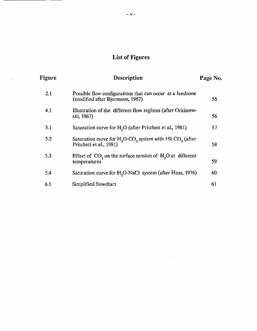
List of Figures
Figure Description Page No.
2.1 Possible flow configurations that can occur at a feedzone(modified after Bjornsson, 1987) 55
4.1 lllustration of the different flow regimes (after Orkiszew-ski, 1967) 56
5.1 Saturation curve for H20 (after Pritchett et a!., 1981) 57
5.2 Saturation curve for ~O-C02 system with 1% CO2(afterPritchett et aI., 1981) 58
5.3 Effect of CO2on the surface tension of ~O at differenttemperatures 59
5.4 Saturation curve for H20-NaCI system (after Haas, 1976) 60
6.1 Simplified flowchart 61
Figure
- Vll-
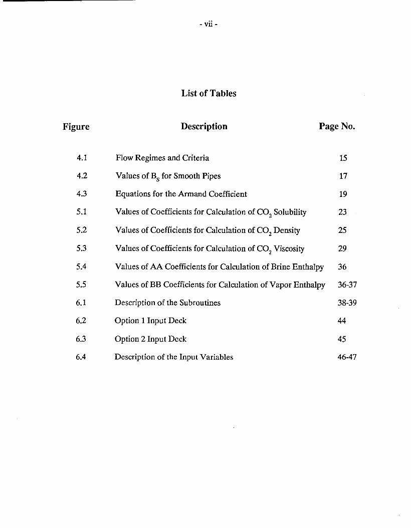
List of Tables
Description Page No.
4.1 Flow Regimes and Criteria 15
4.2 Values of Bs for Smooth Pipes 17
4.3 Equations for the Armand Coefficient 19
5.1 Values of Coefficients for Calculation of CO2 Solubility 23
5.2 Values of Coefficients for Calculation of CO2 Density 25
5.3 Values of Coefficients for Calculation of CO2
Viscosity 29
5.4 Values of AA Coefficients for Calculation of Brine Enthalpy 36
5.5 Values of BB Coefficients for Calculation of Vapor Enthalpy 36-37
6.1 Description of the Subroutines 38-39
6.2 Option 1 Input Deck 44
6.3 Option 2 Input Deck 45
6.4 Description of the Input Variables 46-47
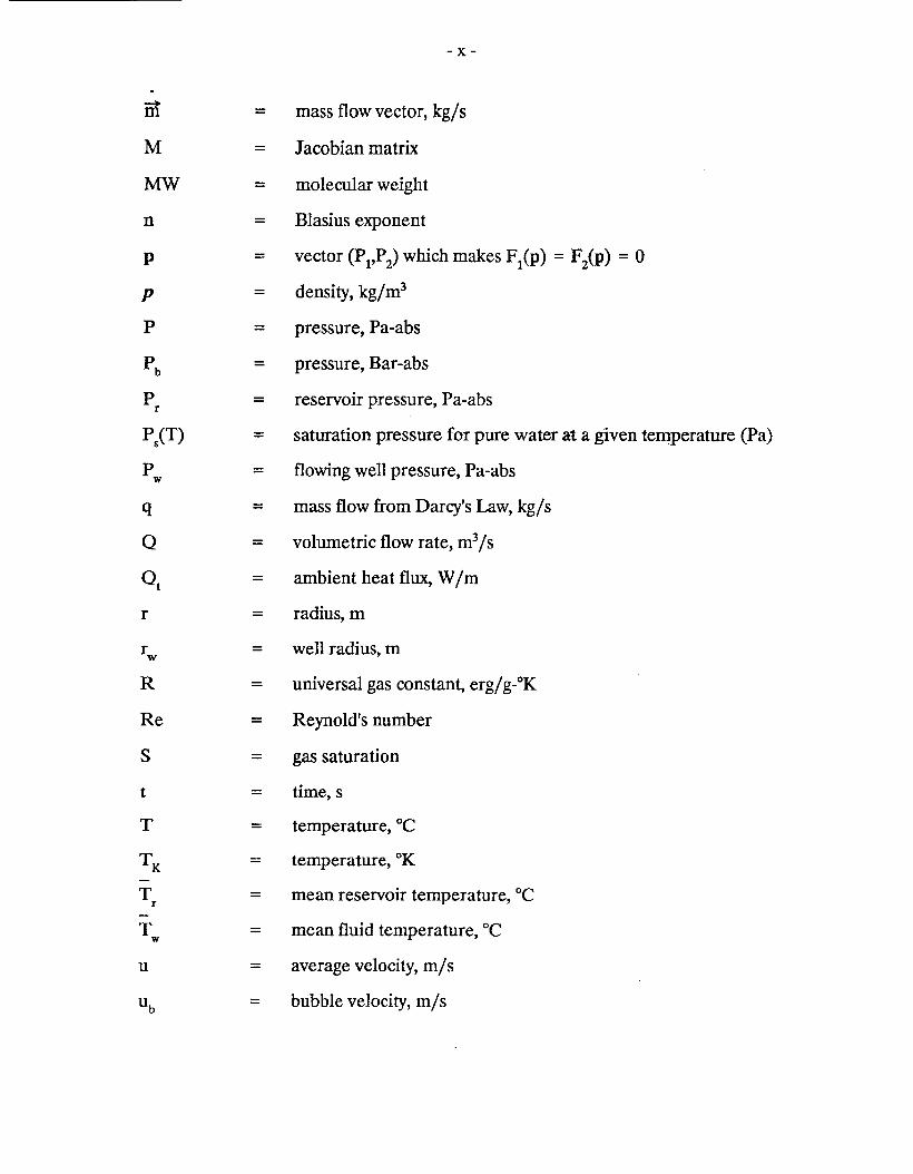
-x-
m = mass flow vector, kg/s
M = Jacobian matrix
MW = molecular weight
n = Blasius exponent
P = vector (Pl'Pz) which makes Ft(p) = F2(p) = 0
p = density, kg/m3
P = pressure, Pa-abs
Pb
= pressure, Bar-abs
P = reservoir pressure, Pa-absr
Ps(T) = saturation pressure for pure water at a given temperature (Pa)
P = flowing well pressure, Pa-absw
q = mass flow from Darcy's Law, kgls
0 = volumetric flow rate, m3Is
°t = ambient heat flux, W1mr = radius, m
r = well radius, mw
R = universal gas constant, erglg-OK
Re = Reynold's number
S = gas saturation
t = time, S
T = temperature, °C
TK = temperature, OK
T = mean reservoir temperature, °Cr
T = mean fluid temperature, °Cw
u = average velocity, mls
~ = bubble velocity, mls
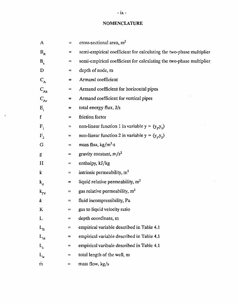
- IX-
NOMENCLATURE
A = cross-sectional area, m2
BR = semi-empirical coefficient for calculating the two-phase multiplier
B = semi-empirical coefficient for calculating the two-phase multipliers
D = depth of node, m
CA = Armand coefficient
CAb = Armand coefficient for horizontal pipes
CAy = Armand coefficient for vertical pipes
Et = total energy flux, 1/s
f = friction factor
F1 = non-linear function 1 in variable y = (yl'y2)
F2 = non-linear function 2 in variable y = (Yl'Y2)
G = mass flux, kg/m2-s
g = gravity constant, m/s2
H = enthalpy, kJ/kg
k = intrinsic permeability, m2
krl = liquid relative permeability, m2
krv = gas relative permeability, m2
k = fluid incompressibility, Pa
K = gas to liquid velocity ratio
L = depth coordinate, m
La = empirical variable described in Table 4.1
~ = empirical variable described in Table 4.1
L = empirical varibale described in Table 4.1s
L = total length of the well, mw
m = mass flow, kg/s

- Xl-
UCH = choked velocity, mls
uH = homogeneous velocity, mls
Ur = Taylor bubble (slug) velocity, mjs
v = specific volume, cm3/g
vc = specific volume of water at the critical point, cm3Ig
v = specific volume of pure water, cm3Ig0
vgD = empirical variable described in Table 4.1
x = mass fraction of. gas
z(Pb,TK) = CO2
compressibility factor
dP
[dLJ ace= pressure drop component due to acceleration, Palm
dP
[dLJ fri= pressure drop component due to friction, Palm
dP
[dLJ JXlI= pressure drop component due to gravity, Palm
dP
[dLJ GO= pressure drop component if fluid flows as liquid only, Palm
dP
[dLJ LO= pressure drop component if fluid flows as gas only, Palm
a = mass fraction of component 2 (i.e. CO2
, NaCl)
fl = dynamic viscosity, kg/m-s
¢FLO = two-phase multiplier
a = surface tension, Nlm
f3 = gas volumetric flow rate ratio
E = pipe roughness, m
1] = Euler's constant
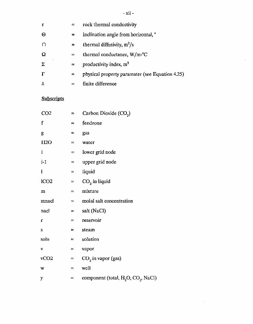
- Xli-
T = rock thermal conductivity
e = inclination angle from horizontal, 0
n = thermal diffusivity, m2/s
Q = thermal conductance, W/m-°C
:I: = productivity index, m3
r = physical property paramater (see Equation 4.25)
t. = finite difference
Subscripts
CO2 = Carbon Dioxide (CO2)
f = feedzone
g = gas
H2O = water
1 = lower grid node
i-I = upper grid node
I = liquid
IC02 = CO2 in liquid
m = mixture
mnad = molal salt concentration
nad = salt (NaCl)
r = reservoir
s = steam
soln = solution
v = vapor
vC02 = CO2
in vapor (gas)
w = well
y = component (total, H,O, CO." NaCl).. ..

- XliI -
ACKNOWLEDGEMENTS
The primary author wishes to thank: the management of PNOC-EDC for the support
extended throughout the course of this project and especially during the final preparation
of this report. Special thanks are due to the whole Reservoir Engineering Staff of
PNOC-EDC who helped with the debugging and validation of the codes. Technical
review of this work by M. J. Lippmann and C. H. Lai is appreciated. This work was par
tially supported by the Assistant Secretary of Conservation and Renewable Energy,
Office of Renewable Energy Technologies, Geothennal Technology Division, of the U.S.
Department of Energy under Contract No. DE-AC03-76SF00098.
1.0 INTRODUCTION
This report describes three multi-component, multi-feedzone geothermal
wellbore simulators developed. These simulators reproduce the measured flowing
temperature and pressure profiles in flowing wells and determine the relative
contribution, fluid properties (e.g. enthalpy, temperature) and fluid composition (e.g.
CO2, NaCl) of each feedzone for a given discharge condition.
The three related wellbore simulators that will be discussed here are HOLA,
GWELL and GWNACL. HOLA is a multi-feedzone geothermal wellbore simulator
for pure water, modified after the wellbore simulator developed by Bjornsson, 1987
and can now handle deviated wells. The other two simulators GWELL (see also
Aunzo, 1990) and GWNACL are modified versions of HOLA that can handle H20
CO2 and H20-NaCI systems, respectively.
These simulators can handle both single and two-phase flows in vertical and
inclined pipes and calculate the flowing temperature and pressure profiles in the well.
The simulators solve numerically the differential equations that describe the steady
state energy, mass and momentum flow in a pipe. The codes allow for multiple
feedzones, variable grid spacing and well radius. These codes were developed using
FORTRAN language on the UNIX system.
1
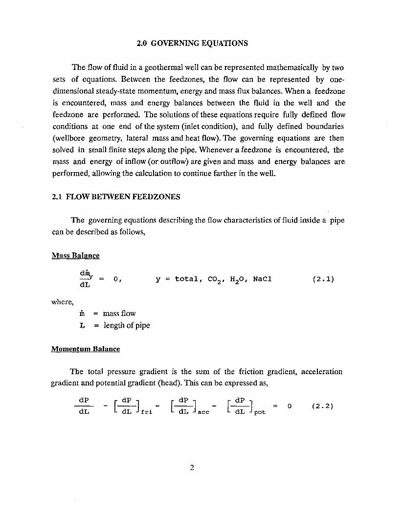
2.0 GOVERNING EQUATIONS
The flow of fluid in a geothermal well can be represented mathematically by two
sets of equations. Between the feedzones, the flow can be represented by one
dimensional steady-state momentum, energy and mass flux balances. When a feedzone
is encountered, mass and energy balances between the fluid in the well and the
feedzone are performed. The solutions of these equations require fully defined flow
conditions at one end of the system (inlet condition), and fully defined boundaries
(wellbore geometry, lateral mass and heat flow). The governing equations are then
solved in small finite steps along the pipe. Whenever a feedzone is encountered, the
mass and energy or inflow (or outflow) are given and mass and energy balances are
performed, allowing the calculation to continue farther in the well.
2.1 FLOW BElWEEN FEEDZONES
The governing equatiops describing the flow characteristics of fluid inside a pipe
can be described as follows,
Mass Balance
d·5 =dL
where,
0, (2.1)
lit = mass flow
L = length of pipe
Momentum Balance
The total pressure gradient is the sum of the friction gradient, accelerationgradient and potential gradient (head). This can be expressed as,
dP
dLdP J
- [dL fri-
2
o (2.2)
where,
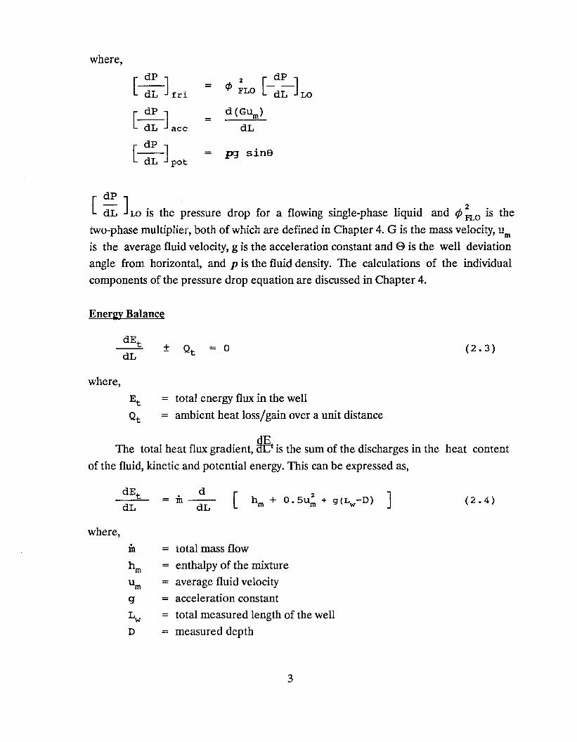
[ :: Jfri2 [dP J= ¢ --FLO dL LO
dP J d (GUm)
[dL ace=
dL
[ :: Jpot= p:J sine
dP
[ dL ] LO is the pressure drop for a flowing single-phase liquid and ¢ ~o is the
two-phase multiplier, both of which are defined in Chapter 4. G is the mass velocity, um
is the average fluid velocity, g is the acceleration constant and E> is the well deviation
angle from horizontal, and p is the fluid density. The calculations of the individual
components of the pressure drop equation are discussed in Chapter 4.
Energy Balance
dEt
dL
where,
(2.3)
Et = total energy flux in the well
Qt = ambient heat loss/gain over a unit distance
The total heat flux gradient, Hft is the sum of the discharges in the heat content
of the fluid, kinetic and potential energy. This can be expressed as,
= total mass flow
= enthalpy of the mixture
= average fluid velocity
= acceleration constant
= total measured length of the well
= measured depth
dEt
dL
where,
in
h m
urng
L wD
. d= m--
dL[ ] (2.4)
3

The ambient heat flux, Qt
in Equation (2.3) is calculated from the heat
conduction equation, representing heat exchange with the rocks surrounding the well,
where,
1
r
oor [ r
oT
or ] =1 oT
-----n ot
(2.5)
T = temperature
r = radial distance from the well
n = rock thermal diffusivity
t = time
The above equation is evaluated assuming that at the well, rw' the temperature is
equal to the wellbore fluid temperature, Tw' and far from the well, the temperature is
equal to the reservoir temperature, Too' such that,
T(rw,t)= TwT(r,O) = Too
T(oo,t) = Too
2An approximate solution can be obtained which is valid when the term nt/rw > >1
(Carslaw and Jaeger, 1959).
where,
TJ = 0.577216... (Euler's constant)
'T = rock thermal conductivityn = rock thermal diffusivity
- 2TJ ] ] -1 (2.6)
Equation (2.6) is only an approximate solution and does not take into account
transient changes in temperature when the well is discharging. Additional heat losses
~~e to convection in the vicinity of the wellbore are also neglected. However, the term
QLt in Equation (2.4) is usually much larger than Qt' and therefore the approximate
solution is reasonable.
4
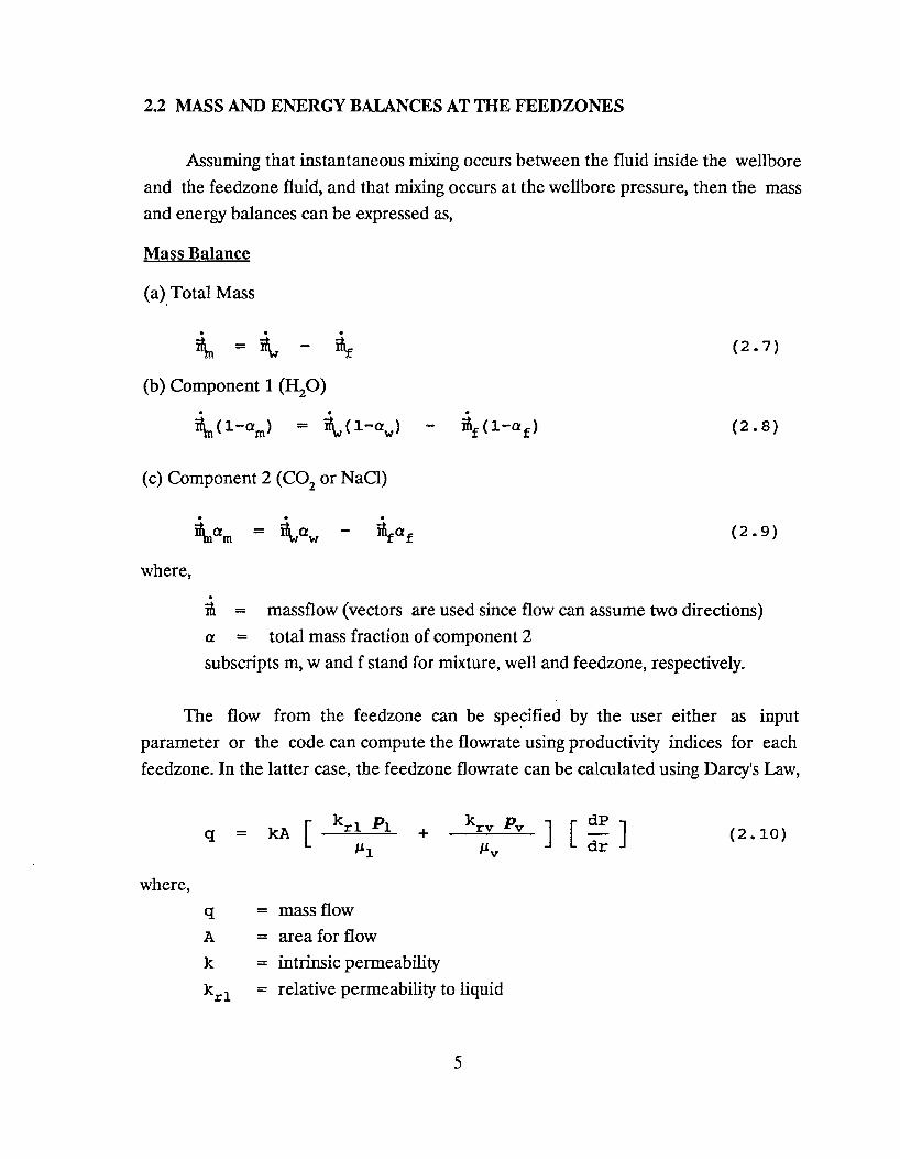
2.2 MASS AND ENERGY BALANCES AT THE FEEDZONES
Assuming that instantaneous mixing occurs between the fluid inside the wellbore
and the feedzone fluid, and that mixing occurs at the wellbore pressure, then the mass
and energy balances can be expressed as,
Mass Balance
(a). Total Mass
. .~ = I\,
(b) Component 1 (~O). .~(l-am) = I\,(l-aw )
(c) Component 2 (C02 or NaCl)
where,
(2.7)
(2.8)
(2.9)
.in = massflow (vectors are used since flow can assume two directions)
a = total mass fraction of component 2
subscripts m, wand f stand for mixture, well and feedzone, respectively.
The flow from the feedzone can be specified by the user either as input
parameter or the code can compute the flowrate using productivity indices for each
feedzone. In the latter case, the feedzone flowrate can be calculated using Darcy's Law,
q = kA [ k r1 Pl+
k rv Pv ] [ :: ] (2.10)1-'1 I-'v
where,q = mass flow
A = area for flow
k = intrinsic permeability
k r1 = relative permeability to liquid
5
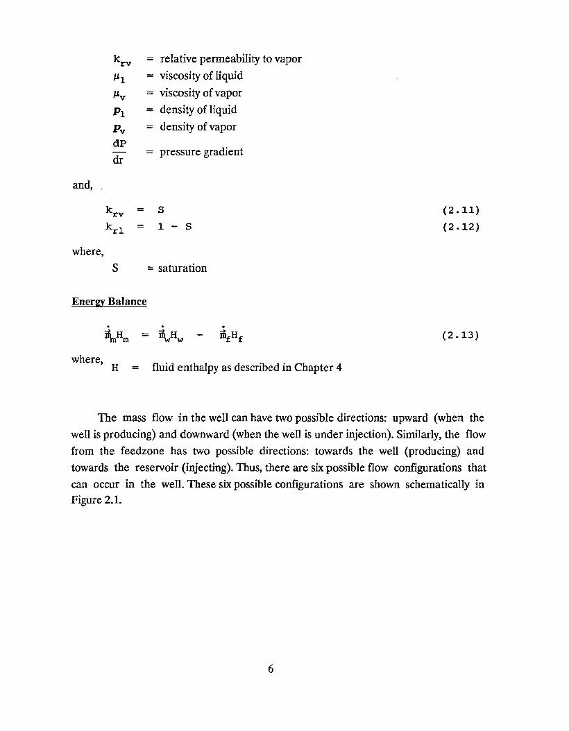
= relative permeability to vapor
= viscosity of liquid
= viscosity of vapor
= density of liquid
= density of vapor
= pressure gradient
and,
k rv = S
k r1 = 1 - s
where,
S = saturation
Ener2;Y Balance
where,H = fluid enthalpy as described in Chapter 4
(2.11)
(2.12)
(2.13 )
The mass flow in the well can have two possible directions: upward (when the
well is producing) and downward (when the well is under injection). Similarly, the flow
from the feedzone has two possible directions: towards the well (producing) and
towards the reservoir (injecting). Thus, there are six possible flow configurations that
can occur in the well. These six possible configurations are shown schematically inFigure 2.1.
6

3.0 NUMERICAL REPRESENTATIONS
The governing differential equations ShOVlll in Chapter 2.0 can be solved
numerically by discretizing the well into finite size grid blocks. The numerical
representations of these equations are given below.
3.1 BElWEEN FEEDZONES
The total pressure drop can be expressed as:
and
o (3.1)
(3.2)
The subscripts i and i-1 refer to the lower and upper grid nodes, respectively, at a
distance L apart. The components of the total pressure drop can be expressed as,
[ ~: Jace =
L1P
[~Jpot =
(GUm)i_l - (GUm)i
L1L
(Pmi-1 sin9i _1 + Pmi sin8J g
2
2
(3.3)
(3.4)
(3.5)
The total energy fllL" at any cross-section in the well is the sum of the heatcontent of the fluid, the kinetic energy and potential energy.
(3.6)
Equations (3.1) and (3.2) give two non-linear equations in terms of twoindependent variables. In the single-phase region, for all the three simulators, the
primary variables chosen are temperature and pressure. However, in the two-phaseregion, pressure and mass fraction of vapor (gas), x, are chosen as the primary
variables for the simulators HOLA and GWNACL. However, unlike for pure water
7

where the two-phase region falls on a single saturation curve, the two-phase region in the
~O-C02 system is bounded by a Pmax and Pmin (see Figure 5.2). In this case, using
temperature and pressure instead of pressure and mass fraction of vapor (gas), X, is
computationally more efficient for the simulator GWELL.
Consider Equations (3.1) and (3.2) as twice differentiable and continuous
functions FI(y) and F2(y) for two variables PI and P2. A solution P=(Pl'P2) which
makes FI(P)=F2(P)=O can be obtained by first guessing y = y. = y(y;,y;). A new
iterative value of y is given by,
* *
[ ~~ J = r Y~ ] M-l r Fl (y ) 1L Y2 L F2 (Y*) ..
where M is the Jacobian matrix:
* *[OF1 (YloFl (y )
]M = oYl °Y2* *oF2(y) of2 (y )
oYl oY2
(3.7)
(3.8)
If a solution P exists and all the first and second derivatives of F 1 and F2 are
bounded, then y will converge quadratically to P.
The derivatives inside the Jacobian matrix are discretized as follows,
* * * *Fl(Yl + Yl 'Y2) - F1 (y1 ,y2)=
Yl(3.9)
where,
y 1 = a small fraction of y;Also, the thermal conductance for each node is calculated as,
o = 4T7[ [ [4nt
In -r 2
w] ]
-1- 2T] (3.10)
The heat loss, 0, can then be computed as,
Q =O(T -if)w r
8
(3.11)

where,
Tw = mean fluid temperature between two adjacent nodes
T r ;: mean reservoir temperature between two adjacent nodes
3.2 AT FEEDZONES
If a feedzone exists at, say node i, the thermodynamic properties of the mixture
are calculated assuming an imaginary node, m, where mixing occurs simultaneously at
a pressure equal to the pressure of node i. The mass flow, enthalpy and composition of
the mixture are then evaluated using Equations (2.7), (2.8) and (2.9) (see Chapter 2.0).
Flow from or into the feedzone can be evaluated by expressing Equation (2.10) as
follows,
=kA
r[ + (3.12 )
Pr and Pware the pressures in the reservoir and well, respectively, and r is the
distance to the reservoir at Pr. The parameter kAI r can be lumped together to form a
group called the Productivity Index, L. The Equation (2.23) can be expressed as,
= L [ + (3.13)
It should be noted that the above definition of the Productivity Index, L, is not
the same as that used in the petroleum industry.
9

4.0 THEORY OF lWO·PHASE FLOW IN VERTICAL AND INCLINED PIPES
4.1 INTRODUCTION
The problem of accurately predicting pressure drop in two-phase flow is difficultsincet two-phase flows are complex and difficult to analyze even for limited conditions
studied. Under some conditions, the gas moves at a much higher velocity than the
liquid. Also, the liquid velocity along the pipe wall can vary appreciably over a short
distance and result in a variable friction loss. Under other conditions, the liquid is
almost completely entrained in the gas and has very little effect on the wall friction
loss. The difference in velocity and the geometry of the two phases strongly influence
pressure drop. These factors provide the basis for categorizing two-phase flows
(Orkiszewski t 1967).
In two-phase flows, it is customary to treat the flow of liquid and gas separatelyusing the well established theory of single-phase flow. These equations are then
extended for two-phase flows using empirical correlations. Here, these empirical
equations are taken from Chisholm (1983). The notations used and the presentation of
the equations are patterned after Bjornsson (1987).
4.2 SINGLE PHASE FLOW
The flow of single-phase fluid in pipes is treated extensively in fluid mechanics
literature. The flow calculations are carried out using linear equations assuming that
the fluid properties remain relatively constant. The components of the total pressure
drop (pressure drop due to friction, potential and acceleration) can be expressed ast
[ :: ] fri
fGZ= (4.1)
4rw p
dP J[~ pot
= pgsine (4.2)
[ :: Jace
d(Gu)(4.3)=
dL
where t
f = friction factor
G = mass velocity
10
r w = well radius
p = density of fluid
g = gravity con~tant
e = deviation angle from horizontal
u = average fluid velocity
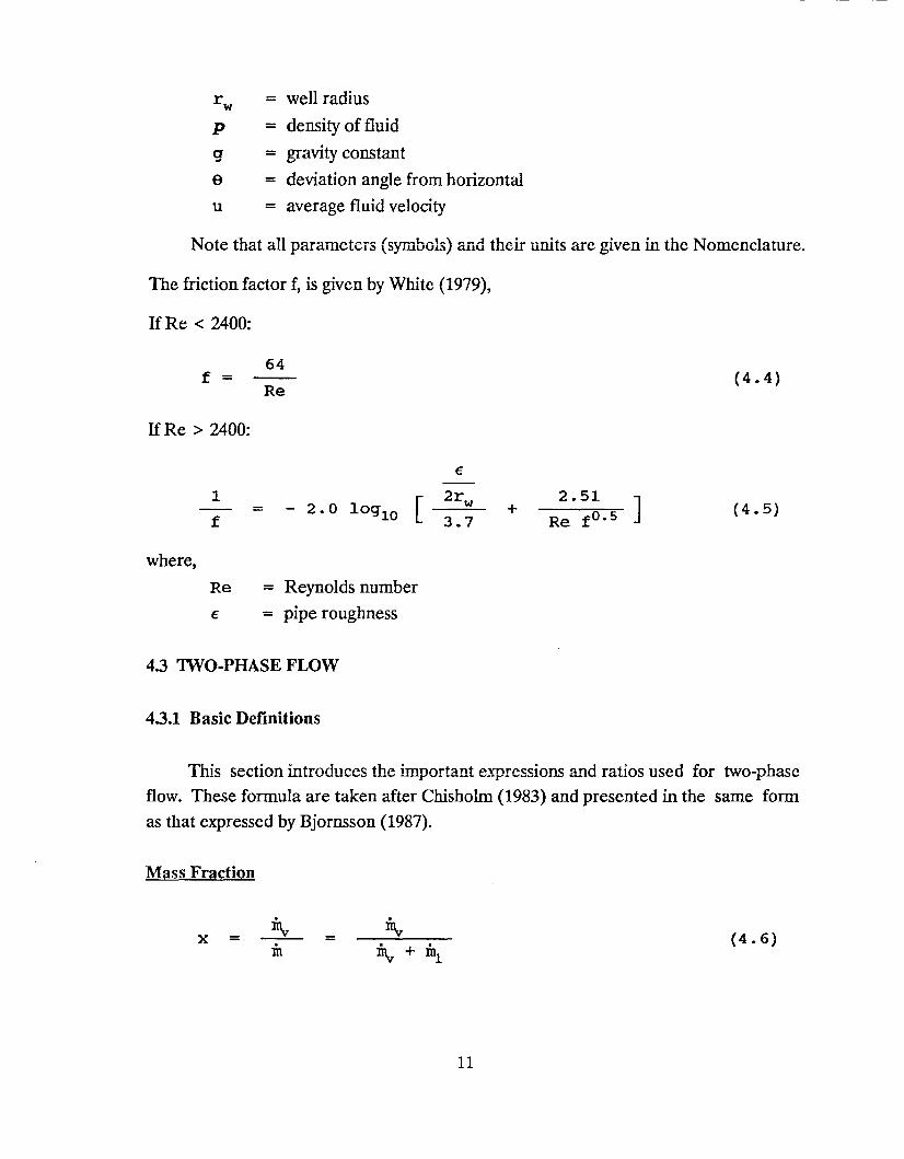
Note that all parameters (symbols) and their units are given in the Nomenclature.
The friction factor f, is given by White (1979),
IfRe < 2400:
f =
IfRe > 2400:
64
Re(4.4)
€
1 [ 2rw 2.51 ]= - 2.0 loglO + (4.5)f 3.7 Re fO.s
where,
Re = Reynolds number
€ = pipe roughness
4.3 1WO·PHASE FLOW
4.3.1 Basic Definitions
This section introduces the important expressions a...l1d ratios used for two-phaseflow. These formula are taken after Chisholm (1983) and presented in the same formas that expressed by Bjornsson (1987).
Mass Fraction
x = .m
=
11
(4.6)
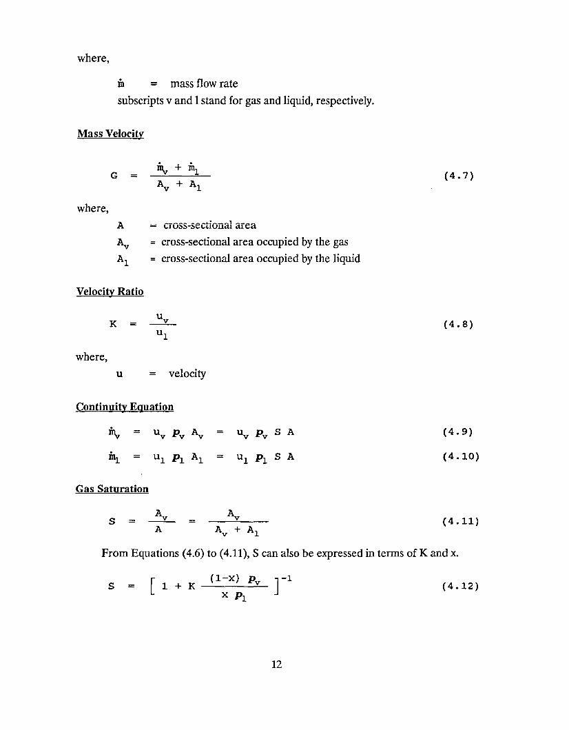
where,
m = mass flow rate
subscripts v and I stand for gas and liquid, respectively.
Mass Velocity
G =
where,
(4.7)
A = cross-sectional area
Av = cross-sectional area occupied by the gas
Al = cross-sectional area occupied by the liquid
Velocity Ratio
where,
K = (4.8)
u = velocity
Continuity Equation
Gas Saturation
(4.9)
(4.10)
s = = (4.11)
From Equations (4.6) to (4.11), S can also be expressed in terms of K and x.
s = [ 1 + K(1-x) Pv
x PI
12
(4.12)

Gas. Liquid and Homogeneous Velocities
Combining Equations (4.6) to (4.11), the following relations can be derived,
[ x K(l-X) ]Uv = G + (4. 13)Pv PI
G r x K(l-X) ]U l = + (4.14 )K L Pv PI
When the velocity ratio, K, is unity, the phase velocities are the same. This
velocity is known as the homogeneous velocity, uH •
[ x (l-X) ]uH = G +Pv PI
Volumetric Flow Rates
x G AQv = Av Uv =
Pvx G A
QI = Ai UI =PI
Gas Volumetric Flowrate Ratio
(4.15 )
(4.16 )
(4.17)
f3 = = [ 1 + 1-x P ]-- -..:!....-
X PI(4.18 )
Density of Mixture
= (4.19)
An alternative expression for the mixture density can be obtained as a function of
the mass fraction, X, and velocity ratio, K By combining Equations (4.12) and (4.19),Pm
can be expressed as,
=x + K(l-x)
[ ~ + K(l-x) ]
Pv PI
13
(4.20)
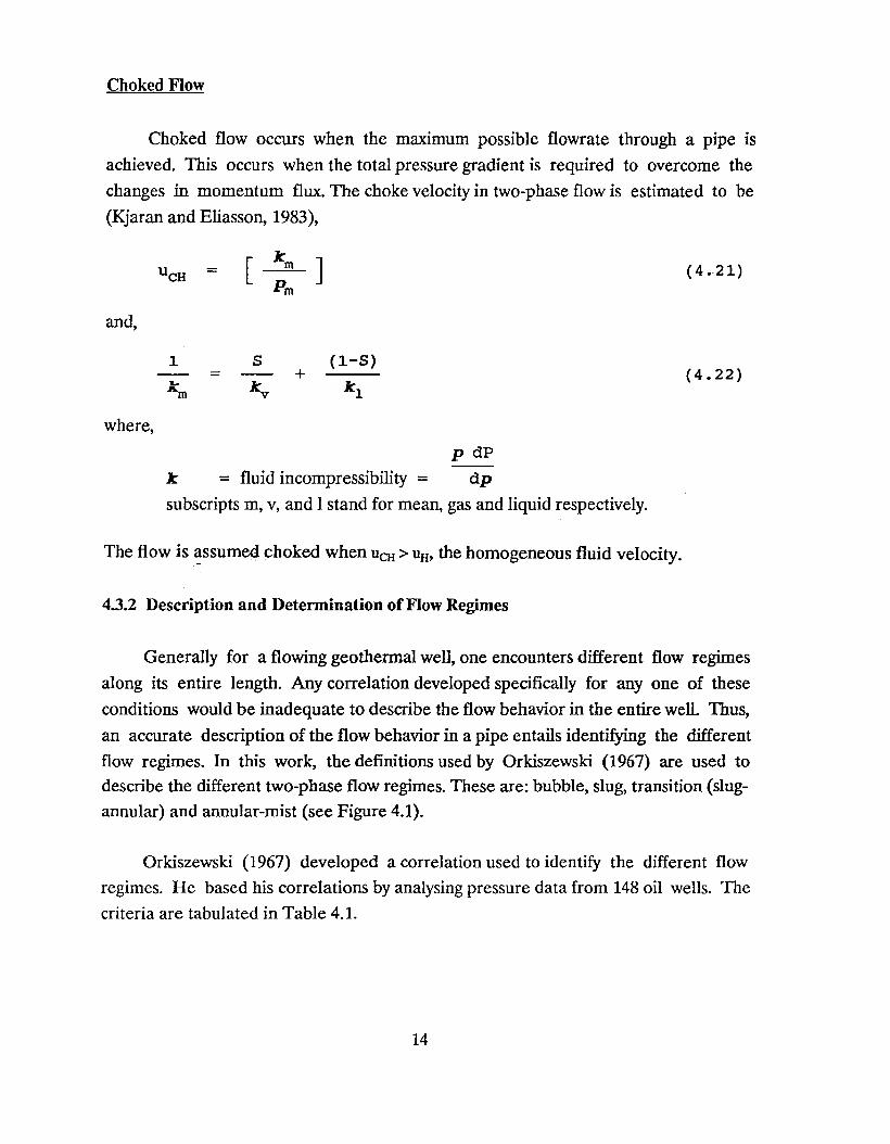
Choked Flow
Choked flow occurs when the maximum possible flowrate through a pipe is
achieved. This occurs when the total pressure gradient is required to overcome the
changes in momentum flux. The choke velocity in two-phase flow is estimated to be
(Kjaran and Eliasson, 1983),
UCB = [~]Pm
and,
1 8 (1-8)= +
Llev le1Am
where,
(4 .. 21)
(4.22)
pdP
Jc = fluid incompressibility = dp
subscripts m, v, and I stand for mean, gas and liquid respectively.
The flow is~ssume<i choked when UCH > UH, the homogeneous fluid velocity.
4.3.2 Description and Determination of Flow Regimes
Generally for a flowing geothermal well, one encounters different flow regimes
along its entire length. Any correlation developed specifically for anyone of these
conditions would be inadequate to describe the flow behavior in the entire well. Thus,
an accurate description of the flow behavior in a pipe entails identifying the different
flow regimes. In this work, the definitions used by Orkiszewski (1967) are used todescribe the different two-phase flow regimes. These are: bubble, slug, transition (slug
annular) and annular-mist (see Figure 4.1).
Orkiszewski (1967) developed a correlation used to identify the different flow
regimes. He based his correlations by analysing pressure data from 148 oil wells. The
criteria are tabulated in Table 4.1.
14

TABLE 4.1
FLOW REGIMES AND CRITERIA (after Bjornsson, 1987)
FLOW REGIME CRITERIA
Bubble 13 < La
Slug 13 > La and V oD < La
Transition La < V oD <~
Mist ~ < V oD
where,
xG[ :~ J
0.25V gD = (a = surface tension)
Pv
[ x (l-x) ]v t = G +Pv PI
v2
La = 1.071 - 0.676__t_
and La > 0.132rw
La = 50 + 36 V gD~
Qv
~0.75
~ = 50 + 36 [ V gD ]Qv
13 =Qv
Q_- + Q1-v
4.3.3 Pressure Drop due to Friction
4.3.3.1 Vertical Pipes
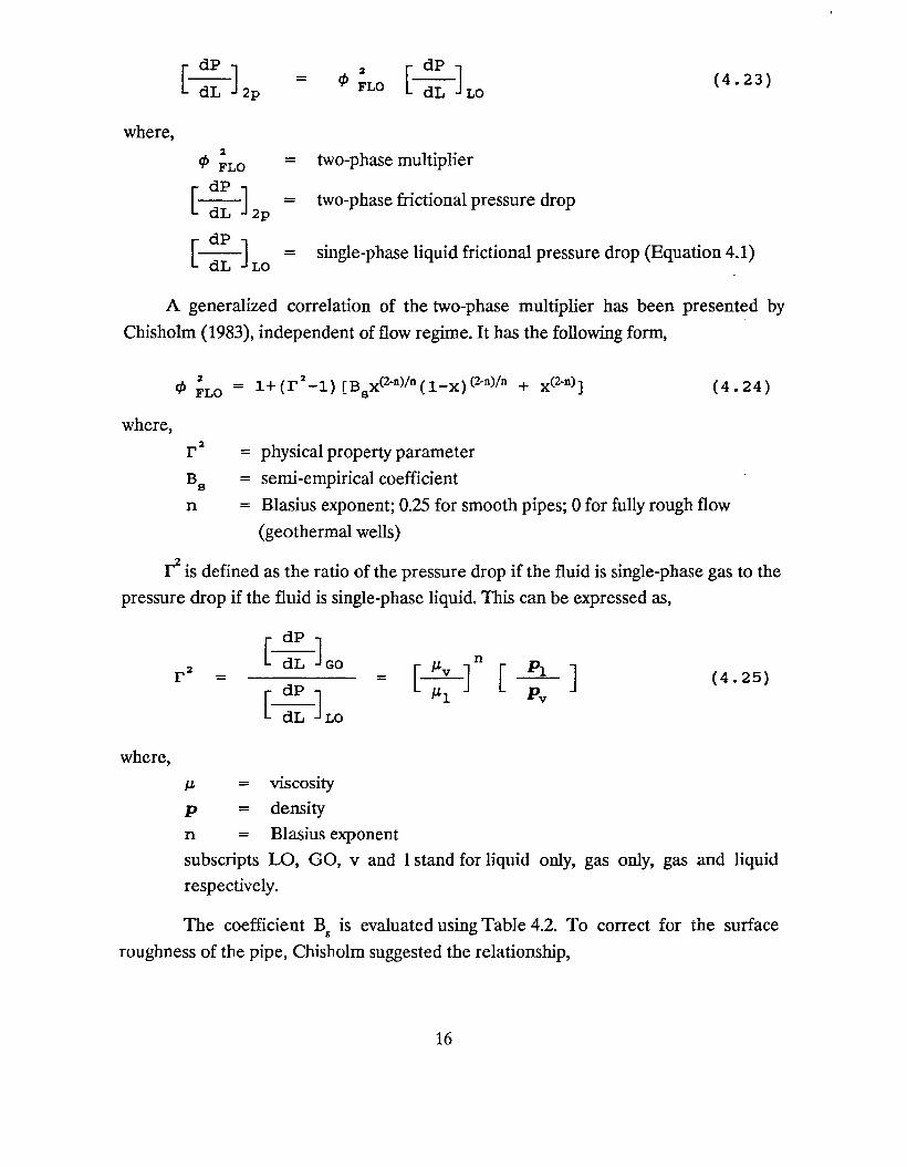
The pressure drop for two-phase flow can be evaluated using the concept of "two
phase multiplier" (Martinelly and Nelson, 1948).
15
where,
= (4.23)
=2
cf> FLO
[ :: J2p =
[::JLO
=
two-phase multiplier
two-phase frictional pressure drop
single-phase liquid frictional pressure drop (Equation 4.1)
A generalized correlation of the two-phase multiplier has been presented by
Chisholm (1983), independent of flow regime. It has the following form,
(4.24)
where,
r 2 =Be =n =
physical property parameter
semi-empirical coefficient
Blasius exponent; 0.25 for smooth pipes; 0 for fully rough flow
(geothermal wells)
r 2is defined as the ratio of the pressure drop if the fluid is single-phase gas to the
pressure drop if the fluid is single-phase liquid. This can be expressed as,
where,
=[~JGO
[ :: JLO
= (4.25)
Jl. = viscosity
P = densityn = Blasius exponentsubscripts LO, GO, v and I stand for liquid only, gas only, gas and liquidrespectively.
The coefficient Bs is evaluated using Table 4.2. To correct for the surface
roughness of the pipe, Chisholm suggested the relationship,
16

~ [~J2 (0.25-0)/0
= [0.5 [1 + + 10(-30(lE/fw) ] ] . (4.26)Bs J1.1
u:,ha.-ra.'t'l'~""..1."'"
€ = pipe roughness
r w = pipe radius
Then for geothermal wells (n=O), Equation (4.24) above can be simplified to,
2
¢ FLO =
TABLE 4.2
(4.27 )
VALVES OF BS FOR SMOOTII PIPES (from Chisholm, 1983)
r G (kg/mz s) Bs:s; 500 4.8
:s; 9.5 500 :s; G :s; 1900 2400/G
~ 1900 55/G~
:s; 600 520/(r G~)9.5 < r < 28
> 600 21/r
~ 28 15000/(rZ G~)
4.3.3.2 Inclined Pipes
For steam-water mixtures Haywood et. al. (1961) obtained a large amount of
data for both horizontal and vertical pipes and found that no significant influence of
pipe inclination was observed.
At present time, no available methods have been found to predict the effect of
inclinaton angle in frictional pressure drop (Chisholm, 1983). Therefore, in this study,
the correlation for vertical pipes was used for inclined pipes.
4.3.4 Velocities of Individual Phases
Two methods are presented here to evaluate the velocities of gas and liquid
phases used in the evaluation of the momentum flux and energy equations. These
methods are based on empirical correlations.
17

4.3.4.1 Armand Correlation
Armand (1946) correlated data for the saturatio~ S, during air/water flow in
pipes. He proposed the relationship,
where,
s = (4.28)
f3 = gas volumetric flowrate ratio, evaluated using Equation (4.18)
CA = Armand Coefficient
Chisholm (1983) reviewed Armand's approach and correlated it with the
results from the work done by Beggs (1972) to include effects of pipe inclination.
He recommended several equations for calculating CA for horizontal, vertical and
inclined pipes. These equations are tabulated in Table 4.3.
4.3.4.2 Orkiszewski Correlation
The phase velocities can also be calculated using the correlations developed
based on the flow regimes as defined by Orkiszewski (1967). The general equation for
the calculation of gas phase velocity is,
(4.29)
Bubble Flow
For this regime, the bubble velocity is evaluated from the correlation given by
Govier and Aziz (1972).
(4.30)
(4.31)
18
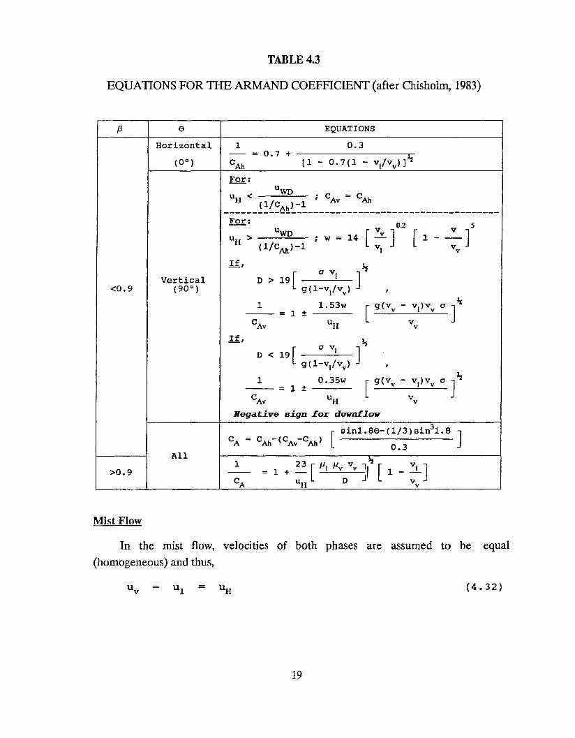
TABLE 4.3
EQUATIONS FOR THE ARMAND COEFFICIENT (after Chisho~ 1983)
f3 e EQUATIONS
1Horizontal 0.3- = 0.7 + -----------,Lr-CAb [1 - 0.7(1 - v l /vv )]'2
For:UWD
u H < ; CAv = CAb
-----_~:~:~~~:_---------------------------------U v 0.2
uH > WD ; w = 14 [~] [1(1/CAb )-1 VI
[ g(Vv - VVI)VV a ] ~
v
1 ±---
D > 19 [ a VI J~9(1-v/vv )
1 1. 53w--=
If,
Vertical(90°)<0.9
If, D < 19 [ a VI ] ~9(1-v/vV>
1 0.35w--=l±---
CAy u H
Negative sign for dovnf1.ov
>0.9
All
Mist Flow
In the mist flow, velocities of both phases are assumed to be equal
(homogeneous) and thus,
= = (4.32)
19

Transition Flow
In the transition regime, a linear interpolation between bubble velocity in slug
and mist flow regimes is used. This is expressed as follows,
where,
= [ (4.33)
U H = homogeneous velocity as defined by Equation (4.15)
ub = bubble velocity
uT = slug velocity
~, vgD and Ls are empirical variables defined in Table 4.l.
Also by combining Equations (4.6), (4.7), (4.9) and (4.0), the expression for the
liquid phase velocity can be derived. The value of ul can be evaluated by solving
simultaneously Equations (4.34) and (4.35) to yield:
G - U P Su 1 = v v (4.34)
Pl(l-S}
G xS = (4.35)
Uy Pv
20

21
5.0 EQUATIONS OF STATE
5.1 WATER-CARBON DIOXIDE SYSTEM (COz-~O)
The mixture C02-~O is of great interest in the analysis of geothermal systems,
since geothermal water often contains a significant amount of COz' Several workers
have looked into the effects of CO2 on the tb.ermodynamics of geothermal fluids.
Sutton (1976) and Sutton and McNabb (1977) have conducted studies on the effect of
CO2
on the boiling CUIVes at Broadlands geothermal field New Zealand. Pritchett et ale
(1981) also looked into the effects of CO2 on the Baca Geothermal Reservoir, New
Mexico. Gaulke (1986) demonstrated the use of CO2 in the evaluation of geothermal
reservoirs.
For pure water, the two-phase region is defined by the loci of points known as the
saturation curve. This is shown in Figure 5.1. H the actual fluid pressure is below the
saturated pressure for a given temperature, then the fluid exists as a single phase
steam. If the fluid pressure is above the saturated pressure at the given temperature,
then the fluid can only exist as liquid water. All two-phase conditions are confined to
lie on the saturation curve.
When CO2 is present, two effects have been found to occur on the region of
the saturation curve (Pritchett et al., 1981). First, the boiling point pressure (pres
sure at which two-phase starts to fonn) for a fixed temperature increases. This
means that if a system consisting of pure water in the compressed-liquid state
undergoes pressure decrease, the fluid will turn two-phase as the saturation pres
sure is reached. If a certain amount of CO2 is present, the pressure at which two
phase starts to form (Pmin) will be greater than the saturation pressure for pure
water. As more CO2 is added, the pressure difference becomes higher. On the
other hand, if a fluid consisting of water and CO2 initially at the gaseous state is
compressed, liquid water will start to form at a particular pressure (Pmax) in the
absence of CO2, this will occur at the saturation pressure. In the presence of CO2,
the pressure at which liquid starts to form was found to be only slightly greaterthan for pure water. Consequently, with the presence of CO2, the boiling pressure
will exceed the condensation pressure (the pressure at which a gaseous mixture
condenses). Both pressures will exceed the saturation pressure for pure watershown as dashed line in Figure 5.2. Figure 5.2 shows a pressure vs. temperature
plot for system containing 1% total mass fracture CO2, The width of the twO
phase region, shown as a shaded area in Figure 5.2 will increase with increasingCO2,
5.1.1 CRITERIA FOR DETERMINING THE STATE OF THE FLUID
Depending upon the value of total pressure, temperature and the total mass
fraction of CO2, the fluid can exist as: (1) an all-liquid solution of CO2 in water, (2) a
mixture of liquid solution and gas, or (3) an all-gas solution of CO2 in steam.
5.1.1.1 All·Liquid Solution of CO2 and ~O
If the total pressure is greater than the saturation pressure of pure water at the
given temperature and the solubility of CO2 in water is greater than the given total
mass fraction of CO2, then the fluid is in the liquid state.
5.1.1.2 Two-Phase
If the total pressure is greater than the saturation pressure of pure water at the
given temperature but the solubility of CO2 in water is less than the given mass fraction
of CO2, then a corresponding gas phase will exist. The fluid then exists in a two-phase
condition.
5.1.1.3 A11·Gas
If the total pressure is less than or equal to the saturation pressure of pure water
at the given temperature and mass fraction of C02' then the fluid can only exist as an
all-gas state.
5.1.2 PARTITIONING OF CO2
BElWEEN LIQUID AND GAS PHASE
Extensive experimental work on the solubility of CO2 in water has been done by
Takenouchi and Kennedy (1964). Ellis and Golding (1963) also investigated the
solubility of CO2 in water and in NaCl solutions of up to 2 molal.
5.1.2.1 Solubility of CO2 in Water
A fit on the data by Takenouchi and Kennedy (1964) was shown by Pritchett et
aI. (1981) to obey the following relationship,
22
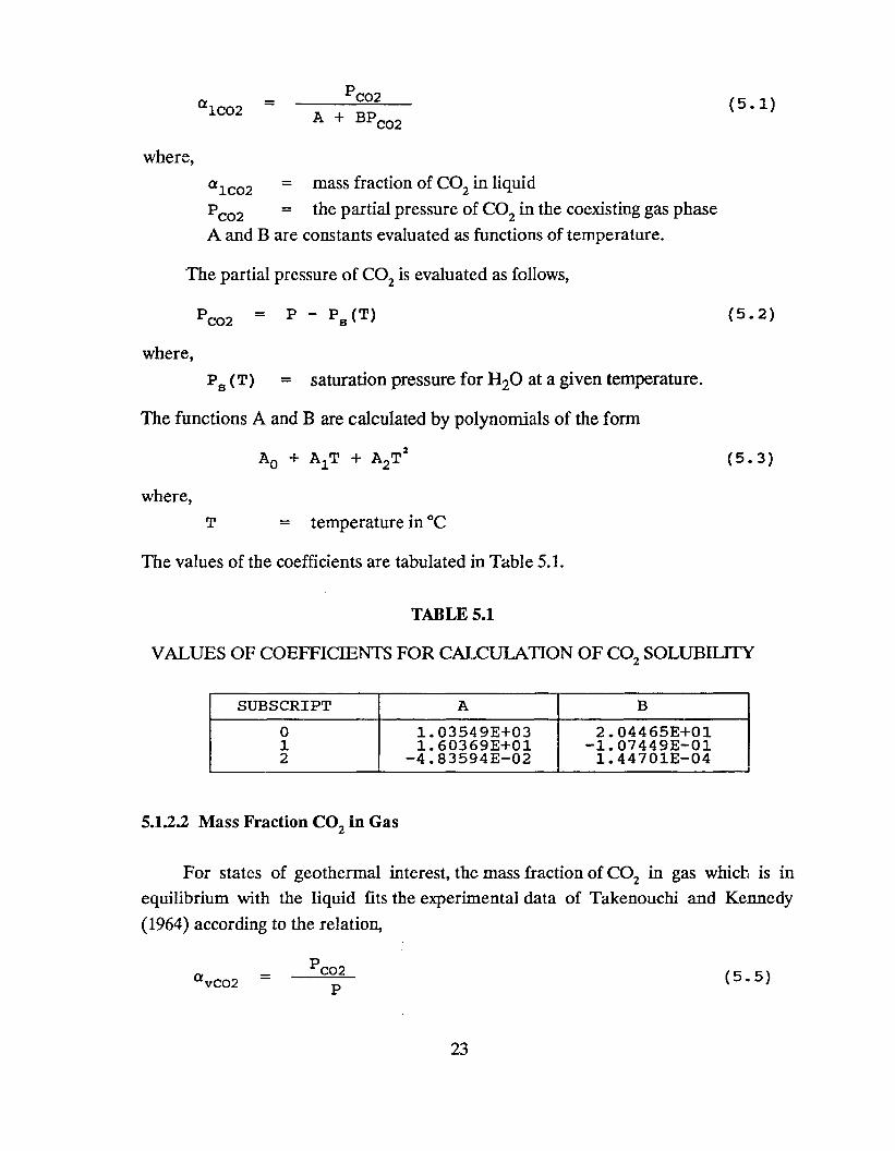
where,
=P C02
A + BPC02(5.1)
(XIC02 = mass fraction of CO2 in liquid
PC02 = the partial pressure of CO2 in the coexisting gas phaseA and B are constants evaluated as functions of temperature.
The partial pressure of CO2 is evaluated as follows,
where,
P C02 = (5.2)
P s (T) = saturation pressure for H20 at a given temperature.
The functions A and B are calculated by polynomials of the form
where,
T = temperature in °C
The values of the coefficients are tabulated in Table 5.1.
TABLES.!
(5.3)
VALUES OF COEFFICIENTS FOR CALCULATION OF CO2
SOLUBILITY
SUBSCRIPT A B
0 1.03549E+03 2.04465E+011 1.60369E+01 -1.07449E-012 -4.83594E-02 1.44701E-04
5.1.2.2 Mass Fraction CO2 in Gas
For states of geothermal interest, the mass fraction of CO2 in gas which is inequilibrium with the liquid fits the experimental data of Takenouchi and Kennedy
(1964) according to the relation,
=P C02
P
23
(5.5)

where,
a VC02
PC02
P
= mass fraction CO2 in gas phase
= partial pressure of CO2 as expressed by Equation (5.2)
= the total pressure
For cases of dry gas (all gas state), the above relation becomes,
=
where,
a C02 = total mass fraction of CO2
(5.6)
Equations 5.5 and 5.6 above fit the experimental data better than Dalton's Law,
which states that the mole fraction of the component gas is proportional to its partial
pressure.
5.1.3 DENSIlY
5.1.3.1 Carbon Dioxide (C02)
The density of CO2 is calculated from the expression obtained from Pritchett et
al. (1981).
PC02 = (5.7)
where,
PC02 =R =T K =Pb =Z (Pb , T K ) =
density of CO2 in kgjm3
the gas constant, 1.88919£6 ergjg-OK
temperature in OK
pressure in bars
gas compressibility factor evaluated using an analytical fit
of the data by Vargaftik (1975).
For pressures less than 300 bars,
z(Pb,TK) = A + B(Pb - 300) + C(Pb - 300)2
+ D(Pb - 300)3 + E(Pb - 300)4
24
(5.8)
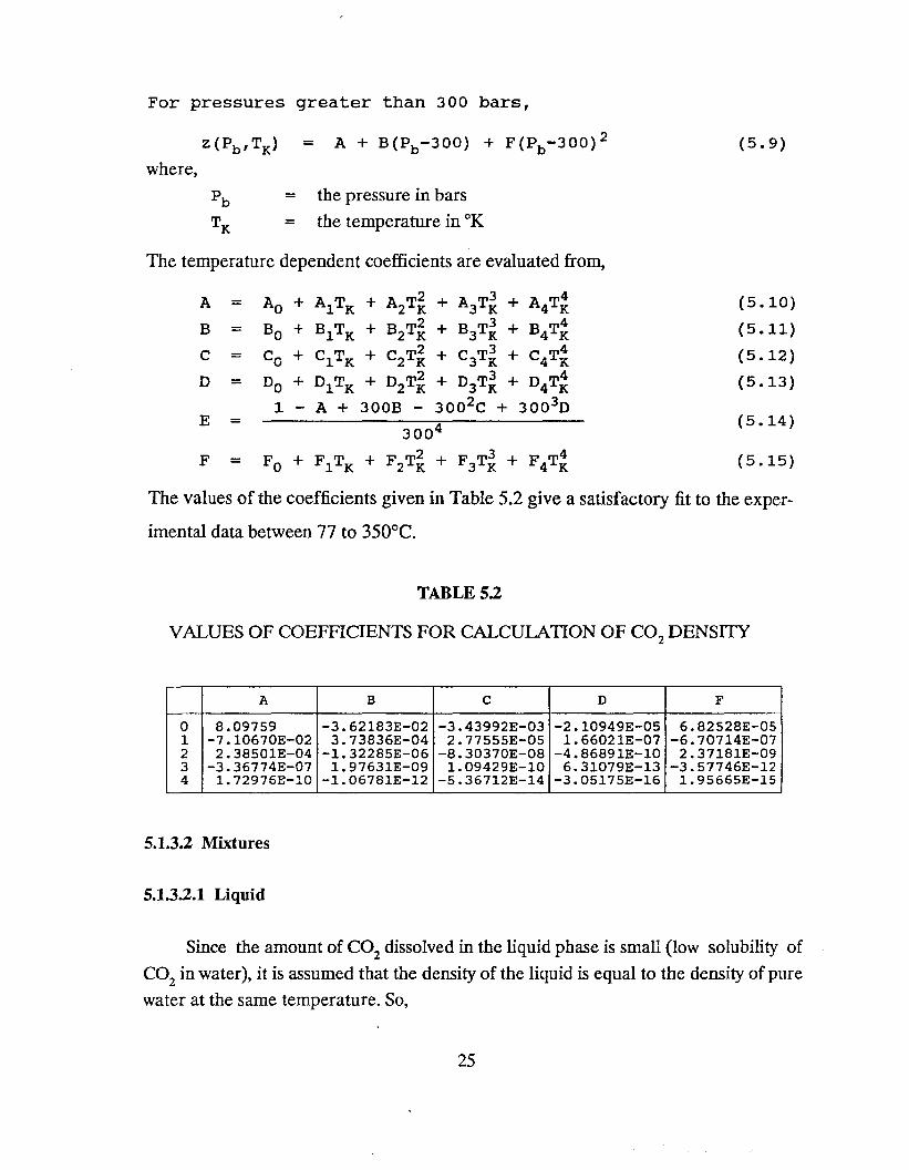
For pressures greater than 300 bars,
Z(Pb,TK) = A + B(Pb-300) + F(Pb-300)2
where,
Pb = the pressure in bars
TK = the temperature in oK
The temperature dependent coefficients are evaluated from,
(5.9)
A Ao + A1TK2 3 4 (5.10)= + A2TK + A3TK + A4TK
B Bo + B1TK2 3 4 (5.11)= + B2TK + B3TK + B4TK
C Co + C1TK2 3 + 4 (5.12)= + C2TK + C3TK C4TK
° DO2 3 4 (5.13)= + 0lTK + 02TK + D3TK + °4TK
1 - A + 300B - 3002C + 30030E =
3004 (5.14)
F Fo + F1TK234 (5.15)= + F 2TK + F3TK + F 4TK
The values of the coefficients given in Table 5.2 give a satisfactory fit to the exper-
imental data between 77 to 350°C.
TABLE 5.2
VALVES OF COEFFICIENTS FOR CALCULATION OF CO2 DENSITY
A B C D F
0 8.09759 -3.62183E-02 -3.43992E-03 -2.10949E-05 6.82528E-051 -7.10670E-02 3.73836E-04 2.77555E-05 1.66021E-07 -6.70714E-072 2.38501E-04 -1. 32285E-06 -8.30370E-08 -4.86891E-IO 2.37181E-093 -3.36774E-07 1. 97631E-09 1.09429E-IO 6.31079E-13 -3.57746E-124 1.72976E-I0 -1. 06781E-12 -S.36712E-14 -3.05175E-16 1.95665E-15
5.1.3.2 Mixtures
5.1.3.2.1 Liquid
Since the amount of CO2 dissolved in the liquid phase is small (low solubility of
CO2
in water), it is assumed that the density of the liquid is equal to the density of pure
water at the same temperature. So,
25
PIwhere,
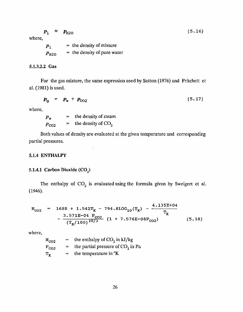
~20 (5.16)
Pi = the density of mixture
PH20 = the density of pure water
5.1.3.2.2 Gas
For the gas mixture, the same expression used by Sutton (1976) and Pritchett et
aI. (1981) is used.
P g = Ps + PC02 (5.17)
where,
Ps = the density of steam
PC02 = the density of CO2
Both values of density are evaluated at the given temperature and corresponding
partial pressures.
5.1.4 ENTHALPY
5.1.4.1 Carbon Dioxide (C02)
The enthalpy of CO2
is evaluated using the formula given by Sweigert et aI.
(1946).
where,
= 1688 + 1.542TK
3.571E-04 PC02(T
K/100) 10/3
4.135E+04
TK(1 + 7.576E-08Pc02 ) (5.18)
HC02 the enthalpy of CO2 in kJ/kg
P C02 = the partial pressure of CO2 in Pa
TK = the temperature in OK
26

(5.19)
5.1.4.2 Heat of Solution
dissolution of the gas in water. The equation of the heat of solution is calculated using
a polynomial fit to the experimental data obtained by Ellis and Golding (1963) and is
valid for temperatures in the range lOO-300°C.
H - -71.33 - 6.0198T + 0.07438T2sain -
- 2.9244E-04T3 + 4.4522E-07T4
where,
= the heat of solution in kJ/kg
= temperature in °C
5.1.4.3 Enthalpy of the Mixture
The enthalpy of the mixture is evaluated using,
= (5.20)
where,
x = mass fraction of gas phase
Hv = enthalpy of the gas phase in kJ/kg
HI = enthalpy of the liquid phase in kJ/kg
The liquid and gas phase enthalpies are evaluated as average enthalpies of the
different components weighted by their individual mass fractions.
HI =
and,
Hv =
where,
(5.21)
(5.22)
a = mass fraction CO2
H = enthalpy, kJ/kg
The subscripts 1, v, w, s, lC02, vC02 and soln stand for liquid phase, gas phase,
water, steam, CO2 in liquid phase, CO2 in gas phase and solution respectively.
27
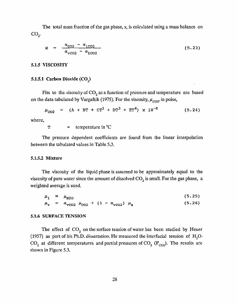
The total mass fraction of the gas phase, X, is calculated using a mass balance on
CO2,
x = Q C02 - Q1C02
QVC02 - Q1C02(5.23)
5.1.5 VISCOSIlY
5.1.5.1 Carbon Dioxide (C02)
Fits to the viscosirj of CO2
as a function of pressure and temperature are based
on the data tabulated by Vargaftik (1975). For the viscosity, Peo2' in poise,
where,
J.LC02 = (5.24)
T = temperature in DC
The pressure dependent coefficients are found from the linear interpolation
between the tabulated values in Table 5.3.
5.1.5.2 Mixture
The viscosity of the liquid phase is assumed to be approximately equal to the
viscosity of pure water since the amount of dissolved CO2 is small. For the gas phase, a
weighted average is used.
=J.LH20
Q VC02 J.LC02 + (1 - a vC02 ) J.Ls
(5.25)
(5.26)
5.1.6 SURFACE TENSION
The effect of CO2
on the surface tension of water has been studied by Heuer
(1957) as part of his Ph.D. dissertation. He measured the interfacial tension of H20
CO2 at different temperatures and partial pressures of CO2 (PCO2)' The results are
shown in Figure 5.3.
28
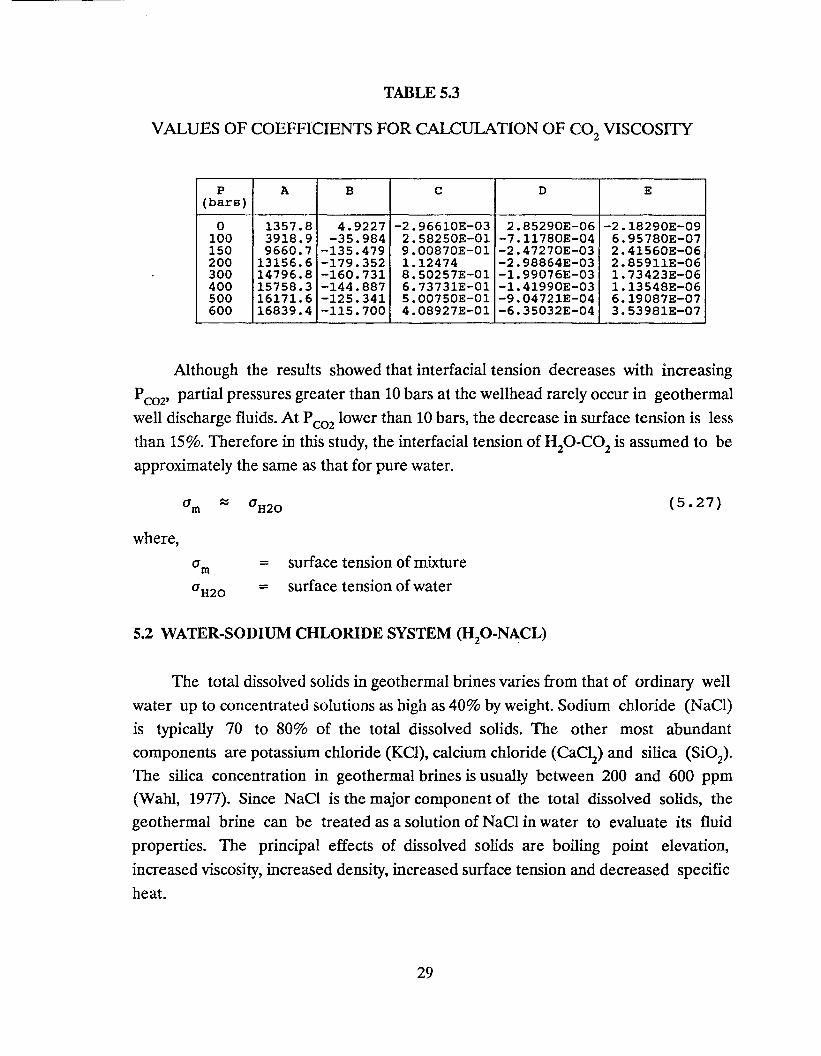
TABLES.3
VALVES OF COEFFICIENTS FOR CALCULATION OF CO2
VISCOSITY
P A B C D E(bars)
0 1357.8 4.9227 -2.96610E-03 2.85290E-06 -2. 18290E-09100 3918.9 -35.984 2.58250E-01 -7. 11780E-04 6.95780E-07150 9660.7 -135.479 9.00870E-01 -2.47270E-03 2.41560E-06200 13156.6 -179.352 1.12474 -2.98864E-03 2.85911E-06300 14796.8 -160.731 8.50257E-01 -1.99076E-03 1. 73423E-06400 15758.3 -144.887 6.73731E-01 -1. 41990E-03 1.13548E-06500 16171.6 -125.341 5.00750E-01 -9.04721E-04 6.19087E-07600 16839.4 -115.700 4.08927E-01 -6.35032E-04 3.53981E-07
Although the results showed that interfacial tension decreases with increasing
Pcoz' partial pressures greater than 10 bars at the wellhead rarely occur in geothermal
well discharge fluids. At Pcozlower than 10 bars, the decrease in surface tension is less
than 15%. Therefore in this study, the interfacial tension of H20-C02 is assumed to be
approximately the same as that for pure water.
(5.27)
where,
(]m = surface tension of mixture
(]H20 = surface tension of water
5.2 WATER-SODIUM CHLORIDE SYSTEM (HzO-NA:CL)
The total dissolved solids in geothermal brines varies from that of ordinary well
water up to concentrated solutions as high as 40% by weight. Sodium chloride (NaCI)
is typically 70 to 80% of the total dissolved solids. The other most abundant
components are potassium chloride (KCI), calcium chloride (CaCI2) and silica (SiOz).
The silica concentration in geothermal brines is usually between 200 and 600 ppm
(Wahl, 1977). Since NaCI is the major component of the total dissolved solids, the
geothermal brine can be treated as a solution of NaCI in water to evaluate its fluid
properties. The principal effects of dissolved solids are boiling point elevation,
increased viscosity, increased density, increased surface tension and decreased specific
heat.
29
5.2.1 CRITERIA FOR DETERMINING THE STATE OF THE FLUID
At a constant pressure, the boiling point temperature of the solution increases as
the salt concentration increases. This is shown in Figure 5.4. Depending upon these
saturation curves, the fluid can exist as single-phase liquid, single-phase gas or two
phase fluid.
5.2.1.1 Single-Phase Liquid
If the total pressure is greater than the saturation pressure at a given temperature
and salt concentration in brine, the fluid is in the liquid state.
5.2.1.2 Two-Phase
If the total pressure is equal to the saturation pressure at a given temperature
and salt concentration in brine, then the fluid is in two-phase condition.
5.2.1.3 Single-Phase Gas
The other remaining case is for single-phase steam. This occurs if the total
pressure is less than the saturation pressure at the given temperature and salt
concentration.
5.2.2 SOLUBILIlY OF NACL IN WATER
The solubility of NaCI in water as a function of temperature is obtained from a
polynomial fit of the data presented by Haas, 1976. The equation is valid for
temperature between 80 to 325°C.
S = 26.218166 + 7.199079E-03 T + 1.060020E-04 T2
(5.28)
where.
s = solubility in wt%T = temperature in DC.
30
5.2.3 SATURATION TEMPERATURE
The boiling point of brine at a given pressure and salt concentration can be
evaluated from the expression given by Haas, 1976. This expression is a fit of the
experimental data between -11 to 300°C.
where,
=In Tsat
a + bTsat(S.29)
To = saturation temperature of pure water pressure, oKTsat = saturation temperature of brine solution, oK.a,b are the coefficients from the polynomial fit.
The coefficients, a and b, are functions of the salt concentration and can be
evaluated using the expression below:
a = I + al(amnacl) + a2(amnacl)2 + a3(amnacl)3
b = bl (amnacl) + b2 (amnacl) 2 + b3 (amnacl) 3
+ b4 (amnacl) 4 + bS (amnacl) 5
where,
amnacl = salt concentration
al = S.93582E-06
a2 = -S.19386E-OS
a3 = 1.23I56E-05
bl = 1.15420E-06
b2 = 1.4I254E-07
b3 = -1.92476E-08
b4 = -1.707I7E-09
b5 = 1.05390E-IO
5.2.4 SATURATION PRESSURE
(S.30)
(5.31)
The vapor pressure of the brine Psat at a given brine temperature T can be cal
culated from (Haas, 1976)
31
e1 e2(10e3w2
In Peat = eO + + - 1. 0)z z
+ e4 10(eS y1.25)(S.32)
where,
Peat = saturation pressure, bars
eO = 12.S0849
e1 = -4.616913E+03
e2 = 3.1934SSE-04
e3 = 1.196SE-11
e4 = -1.013137E-02
eS = -5.7148E-03
e6 = 2.9370E+OS
Y = 647.27 - T0
z = T + 0.0102
e6w = z -To is the equivalent temperature of pure water and can be evaluated from
Equation 5.29 by setting Tsat equal to the brine temperature, T.
5.2.5 DENSIlY
The density of vapor-saturated brine solution is evaluated using the formula
given by Haas, 1976. For compressed liquid, the expression presented by Phillips et at,
1981 is used. For single phase vapor condition, the density is calculated equal to the
density of pure steam at the given temperature and pressure.
Liguid Brine
(a) Vapor-Saturated
where,
=1000 + amnacl MWnac1
1000 vPo + amnacl V nac1
(S.33)
MWnac1 =
==
molecular weight of NaCI
NaCI concentration, molal
specific volume of pure water, cm3/g
V nac1 =
32
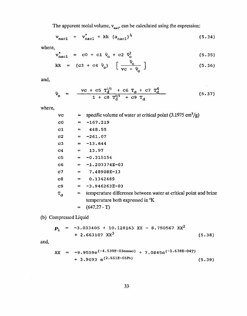
The apparent molal volume, vnacl' can be calculated using the expression:
= (5.34)
where,
v~acl = cO + c1 Vo + c2 ~ (5.35)
kk = (c3 + c4 vol (5.36)
specific volume of water at critical point (3.1975 cm3/g)
-167.219
448.55
-261.07
-13.644
13.97
-0.315154
-1.203374E-03
7.48908E-13
0.1342489
-3.946263E-03
temperature difference between water at critical point and brine
temperature both expressed in OK(647.27 - T)
and,
Vo =
where,
vc =cO =c1 =c2 =c3 =c4 =c5 =c6 =c7 =c8 =c9 =Td =
=
vc + c5 T~3 + c6 Td + c7 T~(5.37)
=
(b) Compressed Liquid
-3.033405 + 10.128163 XX - 8.750567 Xx2
+ 2.663107 XX3
and,
(5.38)
XX = -9. 955ge(-4.539E-03amnacl) + 7.0845e(-1.638E-04T)
+ 3.9093 e(2.SS1E-OSPb) (5.39)
33
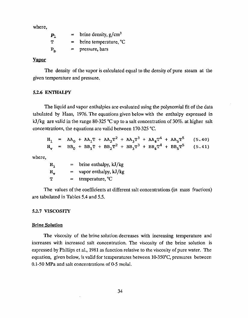
where,
Pl = brine density, g/cm3
T = brine temperature, °c
Pb = pressure, bars
Vapor
The density of the vapor is calculated equal to the density of pure steam at the
given temperature and pressure.
5.2.6 ENTHALPY
The liquid and vapor enthalpies are evaluated using the polynomial fit of the data
tabulated by Haas, 1976. The equations given below with the enthalpy expressed in
kJ/kg are valid in the range 80-325 °c up to a salt concentration of 30%. at higher salt
concentrations, the equations are valid between 170-325 °C.
Hl = AAo + AA1T + AA T2 + AA T3 + AA T4 + AA TS (S.40)2 3 4 5
H = BBo + BB1T + BB2T2 + BB3T3 + BB4T4 + BBsTS (S.41)y
where,
Hl = brine enthalpy, kJ/kg
Hy = vaporenthalpy,kJ/kg
T = temperature, °C
The values of the coefficients at different salt concentrations (in mass fractions)
are tabulated in Tables 5.4 and 5.5.
5.2.7 VISCOSITY
Brine Solution
The viscosity of the brine solution decreases with increasing temperature and
increases with increased salt concentration. The viscosity of the brine solution is
expressed by Phillips et al., 1981 as function relative to the viscosity of pure water. The
equation, given below, is valid for temperatures between 1O-350°C, pressures between
0.1-50 MPa and salt concentrations of 0-5 molal.
34

1 + O.0816amnac1+ O.0122a~aCl+ 1.28E-04a:maCl
where,
-.!!L.J..LH20
=
+ h_?QF._04Tr1_e(-O.7amnacl),- ----~ ---L-- - ... (5.42)
Vapor
====
viscosity of brine, kgjm-s
viscosity of pure water, kgjm-s
temperature, °C
salt concentration, molal
Viscosity of the vapor is taken to be equal to the viscosity of pure steam at the
given temperature and pressure.
5.2.8 SURFACE TENSION
In an ionic solution, the increased electrostatic forces resulting from the ions willincrease the forces of attraction on the surface layers of water molecules, thus
increasing the surface tension of an ionic salt solution. The surface tension of the brine
solution can be calculated using the formula presented below (Wahl, 1977):
a = O.00757(374.15-T)o.776(1+0.0039Wt+4.35E-05W~)
where,
a = surface tension, dyne j cm
T = temperature, °C
wt = salt concentration, wt%
35
(5.43)
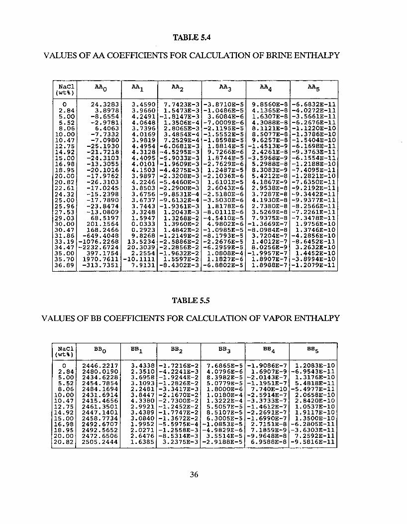
TABLES.4
VALVES OF AA COEFFICIENTS FOR CALCULATION OF BRINE ENTHALPY
NaCl AAO AA1 AA2 AA3 AA4 AA5(wt%)
0 24.3283 3.4590 7.7423E-3 -3.8710E-5 9.8560E-8 -6.6832E-ll2.84 3.8978 3.9660 1. 5473E-3 -1.0486E-5 4.1365E-8 -4.0272E-115.00 -8.6554 4.2491 -1. 8147E-3 3.6084E-6 1.6307E-8 -3.5661E-ll5.52 -2.9781 4.0648 1.3506E-4 -7.0009E-6 4.3088E-8 -6.2676E-ll8.06 6.4063 3.7396 2.8065E-3 -2. 1195E-5 8.1121E-8 -1. 1220E-10
10.00 -7.7332 4.0169 3.4854E-4 -1.5552E-5 8.5077E-8 -1.3786E-1010.47 -7.0980 3.9819 7.2529E-4 -1.8598E-5 9.6257E-8 -1. 5404E-I012.75 -25.1930 4.4954 -6.0681E-3 1.8814E-5 -1. 4513E-9 -6. 1698E-ll14.92 -21. 7218 4.3128 -4.5295E-3 9.7266E-6 2.4261E-8 -9.3763E-ll15.00 -24.3103 4.4095 -5.9033E-3 1.8744E-S -3.5968E-9 -6.1554E-ll16.98 -13.3055 4.0101 -1. 9609E-3 -2.7629E-6 5.2988E-8 -1. 2188E-I018.95 -20.1016 4.1503 -4.4275E-3 1.2487E-5 8.3083E-9 -7.4095E-ll20.00 -17.9762 3.9897 -2.3208E-3 -2.1036E-6 5.4212E-8 -1.2821E-I020.82 -26.3103 4.2246 -5.4460E-3 1. 6101E-5 4.1867E-9 -7.6350E-ll22.61 -17.0245 3.8503 -2.2900E-3 2.6043E-6 2.9538E-8 -9.2192E-ll24.32 -15.2398 3.6756 -9.8531E-4 -2.5180E-6 3.7287E-8 -9.3442E-ll25.00 -17.7890 3.6737 -9.6132E-4 -3.5030E-6 4.1930E-8 -9.9377E-ll25.96 -23.8474 3.7443 -1. 9361E-3 1.8178E-6 2.7380E-8 -8.2566E-ll27.53 -13.0809 3.3248 1.2043E-3 -8.0111E-6 3.5269E-8 -7.2261E-ll29.03 68.5197 1. 5947 1. 3268E-2 -4.5410E-5 7.9375E-8 -7.3478E-ll30.00 201.1564 0.0333 1. 3960E-2 4.9802E-6 -1.3669E-7 1. 9756E-1030.47 168.2466 0.2923 1.4842E-2 -1.0985E-5 -8.0984E-8 1. 3746E-I031.86 -649.4048 9.8268 -1.2149E-2 -8.1793E-5 3.7204E-7 -4.2856E-I033.19 -1076.2268 13.5234 -2.5886E-2 -2.2676E-5 1.4012E-7 -8.6452E-ll34.47 -2232.6724 20.3039 -2.2856E-2 -6.2959E-5 8.0256E-9 3.2632E-I035.00 397.1754 2.2554 -1. 9632E-2 1.0808E-4 -1.9957E-7 1.4452E-I035.70 1970.7611 -10.1111 1.5597E-2 1. 1827E-6 1.8907E-7 -3.8994E-I036.89 -313.7351 7.9131 -8.4302E-3 -6.8802E-5 1.8988E-7 -1.2079E-11
TABLES.S
VALVES OF BB COEFFICIENTS FOR CALCVLATION OF VAPOR ENTHALPY
NaCl BBO BB1 BB2 BB3 BB4 BBS(wt%)
0 2446.2217 3.4338 -1.7216E-2 7.6865E-5 -1.9086E-7 1.2083E-I02.84 2480.0190 2.3510 -4.2241E-3 4.0796E-6 1.6907E-9 -6.9543E-115.00 2434.6228 3.6958 -1.9244E-2 8.3982E-5 -2.0143E-7 1. 3176E-105.52 2454.7854 3.1093 -1.2826E-2 5.0779E-5 -1. 1951E-7 5.4818E-118.06 2484.1694 2.2481 -3.3417E-3 1.8000E-6 7.740E-10 -5.4977E-11
10.00 2431. 6914 3.8447 -2.1670E-2 1.0180E-4 -2.5914E-7 2.0658E-1010.47 2415.4656 4.3380 -2.7300E-2 1.3222E-4 -3.3733E-7 2.8420E-1012.75 2461.3501 2.9921 -1.2452E-2 5.5057E-5 -1.4612E-7 1. 0537E-1014.92 2447.1401 3.4389 -1. 7747E-2 8.5107E-5 -2.2691E-7 1. 9117E-I015.00 2458.7734 3.0840 -1. 3672E-2 6.3005E-5 -1. 6990E-7 1. 3500E-1016.98 2492.6707 1.9952 -5.5975E-4 -1.0853E-5 2.7151E-8 -6.2805E-1118.95 2492.5652 2.0271 -1.2558E-3 -4.9829E-6 7.1859E-9 -3. 6303E-1120.00 2472.6506 2.6476 -8.5314E-3 3.5514E-5 -9.9648E-8 7.2592E-ll20.82 2505.2444 1.6385 3.2375E-3 -2.9188E-5 6.9588E-8 -9. 5816E-11
36
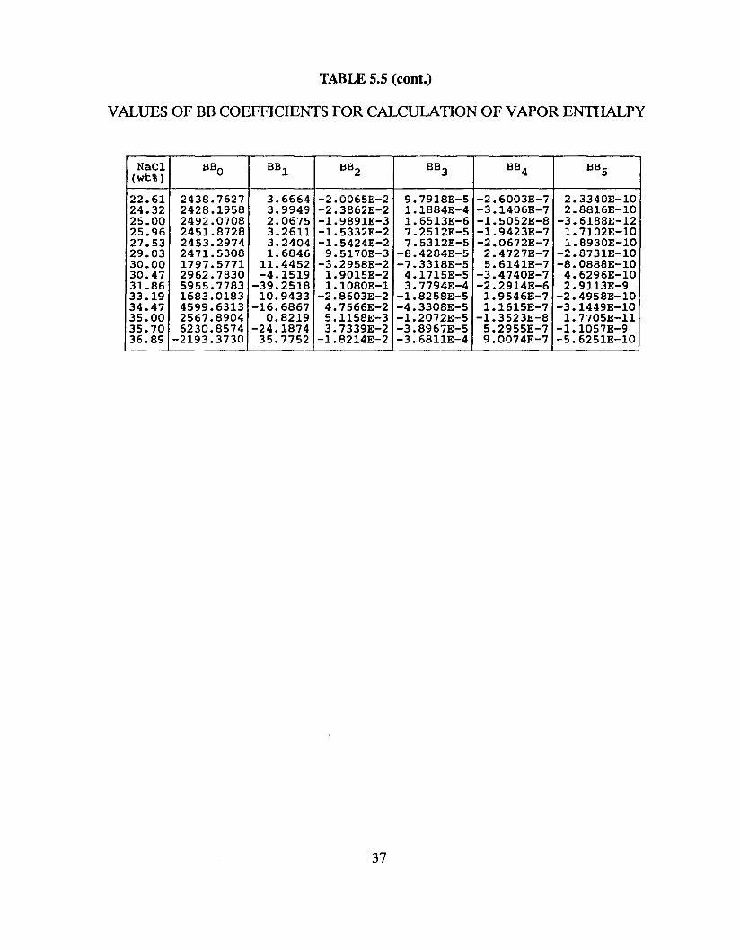
TABLE 5.5 (cont.)
VALUES OF BB COEFFICIENTS FOR CALCULATION OF VAPOR ENTHALPY
NaCl BBO BB1 BB2 BB3 BB4 BB5(wt\>
22.61 2438.7627 3.6664 -2.0065E-2 9.7918E-5 -2.6003E-7 2.3340E-1024.32 2428.1958 3.9949 -2.3862E-2 1.1884E-4 -3.1406E-7 2.8816E-1025.00 2492.0708 2.0675 -1.9891E-3 1.6513E-6 -1. 5052E-8 -3. 6188E-1225.96 2451.8728 3.2611 -1. 5332E-2 7.2512E-5 -1.9423E-7 1. 7l02E-1027.53 2453.2974 3.2404 -1.5424E-2 7.5312E-5 -2.0672E-7 1. 8930E-1029.03 2471. 5308 1. 6846 9.5170E-3 -8.4284E-5 2.4727E-7 -2.8731E-1030.00 1797.5771 11.4452 -3.2958E-2 -7.3318E-5 5.6141E-7 -8.0888E-1030.47 2962.7830 -4.1519 1.9015E-2 4.1715E-5 -3.4740E-7 4. 6296E-1031.86 5955.7183 -39.2518 1.1080E-1 3. 7194E-4 -2.2914E-6 2.9113E-933.19 1683.0183 10.9433 -2.8603E-2 -1.8258E-5 1. 9546E-7 -2.4958E-1034.47 4599.6313 -16.6867 4.7566E-2 -4.3308E-5 1. 1615E-7 -3. 1449E-1035.00 2567.8904 0.8219 5. 1158E-3 -1.2072E-5 -1. 3523E-8 1.7705E-ll35.70 6230.8574 -24.1874 3.7339E-2 -3.8967E-5 5.2955E-7 -1.1057E-936.89 -2193.3730 35.7752 -1. 8214E-2 -3. 6811E-4 9.0074E-7 -5.6251E-I0
37
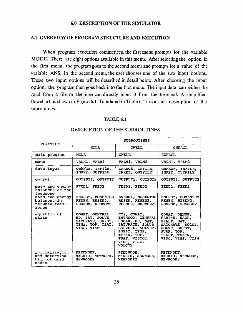
6.0 DESCRIPTION OF THE SIMULATOR
6.1 OVERVIEW OF PROGRAM STRUCTIJRE AND EXECUTION
When program execution commences, the first menu prompts for the variable
MODE. There are eight options available in this menu. After selecting the option in
the first menu, the program goes to the second menu and prompts for a value of the
variable ANS. In the second menu, the user chooses one of the two input options.
These two input options will be described in detail below. After choosing the input
option, the program then goes back into the first menu. The input data can either be
read from a file or the user can directly input it from the terminal. A simplified
flowchart is shown in Figure 6.1. Tabulated in Table 6.1 are a short description of the
subroutines.
TABLE 6.1
DESCRIPTION OF THE SUBROUTINES
SUBROUTINESFUNCTION
BOLA GWELL GWNACL
main program BOLA GWELL GWNACL
menu VALM1, VALM2 VALM1, VALM2 VALM1, VALM2
data input CHANGE, INFILE, CHANGE, INFILE, CHANGE, INFILE,INKEY, OUTFILE INKEY, OUTFILE INKEY, OUTFILE
output OUTPUT1, OUTPUT2 OUTPUT1, OUTPUT2 OUTPUT1, OUTPUT2
mass and energy FEED1, FEED2 FEED1, FEED2 FEED1, FEED2balances at thefeedzonemass and ~nergy ENERGY, MOMENTUM ENERGY, MOMENTUM ENERGY, MOMENTUMbalances ~n RESEN, RESEN2, RESEN, RESEN2, RESEN, RESEN2,between feed- RESMOM, RESMOM2 RESMOM, RESMOM2 RESMOM, RESMOM2zones
equation of COWAT, GENERAL, CO2, COWAT, COWAT, DENSE,state BP, SAT, SOLVE, ENTBC02, GENERAL BBRINE, NACL,
SATURATE, SUPST, BSOLN, MU, SAT, PSALT, SAT,TENS, TOP, TSAT, SATURATE, SOLUB, SATURATE, SOLUB,VISS, VISW SOLVEPX, SOLVET, SOLVE, SUPST,
SUPST, TENS, SURF, TOP,TFIND, TOP, TSALT, TSATN,TSAT, VISC02, VISC, VISS, VISWVISS, VISW,VOLC02
initialization FEEDNODE, FEEDNODE, FEEDNODE,and determina- MKGRID, NEWNODE, MKGRID, NEWNODE, MKGRID, NEWNODE,tion of grid NEWNODE2 NEWNODE2 NEWNODE2nodes
38

TABLE 6.1 (cont.)
nESCRIPTION OF THE SUBROUTINES
SUBROUTINESFUNCTION
HOLA GWELL GWNACL
determination ARMAND, CHOKED, ARMAND, CHOKED, ARMAND, CHOKED,of flow regimes FRICl, MOODY, FRICl, MOODY, FRICl, MOODY,and flow cha- REGIME REGIME REGIMEracteristics
iteration ITl, IT2, IT3, ITl, IT2, IT3, ITl, IT2, IT3,routines IT4, ITERATEl, IT4, ITERATEl, IT4, ITERATEl,
I TERATE2 , ITERATE2, ITERATE2,ITERATE3, ITERATE3, ITERATE3,I TERATE4 , ITERATE4, ITERATE4,ITHEAD, VINNAl, ITHEAD, VINNAl, ITHEAD, VINNA1,VINNA2 VINNA2 VINNA2
sorting routine PLOTTA PLOTTA PLOTTAfor plotting
(1) Option 1 (ANS =1)
This option needs the measured or known discharge condition at t~e wellhead
(e.g. pressure, mass fraction CO2, temperature and enthalpy). In addition, the flow
rates and enthalpies of the feedzones are specified. Take note that for this option the
last feedzone (at bottomhole) may not be specified since the program automatically
calculates the condition of the last feedzone. The simulator then solves for the flowing
temperature and pressure profile from the wellhead to bottomhole. The results can
then be matched with the measured flowing temperature and pressure surveys to
determine the relative contribution and fluid composition from the different feedzones.
(2) Option 2 (ANS=2)
In this option, the user specifies the required flowing wellhead pressure and
bottomhole pressure, and the productivity indeces (defined in Chapter 3),
thermodynamic properties and composition of the fluid at each feedzone. The
simulator then calculates for the flowing temperature and pressure from bottomhole
to the wellhead and calculates the expected wellhead output (e.g. wellhead enthalpy,
fIowrate, pressure, temperature and fluid composition). For this option, unlike the
input for option 1, all the feedzones have to be specified. This program can be used to
39
predict outputs of newly drilled wells using the parameters obtained from neighboring
wells.
These three simulators have two major iteration subroutines that solve for thetemperature and pressure in the well. Option 1 uses the subroutine VINNA1 and
option 2 uses the subroutine ITHEAD.
(1) VINNA1
This subroutine calculates for the pressure, temperature and saturation profiles
of a flowing well given the wellhead conditions and flowrate and enthalpy of each
feedzone. The calculations proceed from the wellhead down to the bottom of the well.
(2) ITHEAD
This subroutine calculates for the flowrate and temperature at the wellhead given
the required wellhead pressure. The productivity index, reservoir pressure and
enthalpy (or temperature) at each feedzone have to be specified. The program will
then compute for the flow contributions from each feedzone using Equation 3.13.
After the input data are read by the program, the calculations proceed using the
equations as discussed in Chapter 3 and using either Orkizewski or Armand
correlation. During the iteration procedure, negative temperatures or pressures are
sometimes calculated if the flow is changing phase. This makes the program return to
the previous node and add a new node to the grid, halfway between the previous node
and the node where the unsuccessful iteration occurred.
The program execution may also be prematurely halted before the calculationreaches the bottom (or top) of the well. This happens for several reasons:
(1) The program computes an impossible thermodynamic condition (e.g. negative
temperature, pressure or mass fraction CO2 or NaCI).
(2) Fluid is above critical condition.
(3) Error in iteration.
(4) Unsuccessful iteration.(5) The simulator calculates velocities in the well more than twice the choke velocity.(6) The specified number of grid nodes is more than 400.
40
In all these cases, error messages will be printed on the screen and on the file
called HOLALOG, GWELL.LOG or GWNACL.LOG depending <?n which simulator
was used. If Option 2 is used additional messages are printed both on the screen and in
the file called *.ITER (* indicates the name of the simulator used). This file contains
data regarding the iteration process.
Mer a successful run, the program goes back to the first menu. The user can
then save the results into a file. Take note that the subroutine PLaTTA (used for
sorting the output for plotting) prompts for a file name, thus the user should first save
the results into a file (Option 6) before sorting can be done (Option 7).
The subroutine PLOTTA creates five files. These are:
1 pvsz.dat
2 tvsz.dat
3 geom.dat
4 fzon.dat
5 flpt.dat
- this file has two columns. The first column contains thecalculated pressure in MPa-gauge and the second column
conatins the corresponding depth in the well in meters.
- this file contains temperature in °C (first column) and the
corresponding depth in meters (second column).
- contains the casing design. The first column is the well radius
in centimeters and the second column is corresponding depth
in meters.
- contains the location of the feedzones in the well. The first
column is the location of the x-axis where the point is to be
plotted (set = 0). The second column is the depth in the well,
in meters, where the feedzone is located.
- contains the location where phase change occurs in the well.The first column is the location of the x-axis where the pointis to be plotted (set = 0). The second column is the depth atwhich a phase change occurs.
Take note that the subroutine PLaTTA is only a sorting program and can be
changed or modified to tailor the output of the subroutine to a specific plotting
software that the user might be using.
41
6.2 INPUT DATA
The input data can either be read from a file or can directly be inputted through
the keyboard. In case changes in the data are needed, the user can either use the
system editor to edit the file, or he can read the file and input the necessary corrections
directly from the keyboard. The program also provides an option to save the edited
input deck when inputting or changes were done interactively.
The structure of the input files for Options 1 and 2 are described below. The
variables can be specified in either F or E format as long as the variables in a line are
separated by at least a space. Samples of the input deck, output and message files
(* .LOG and *.ITER) are attached in Appendix A Positive flows at the wellhead or
feedzones indicate production and negative flows indicate injection. In the well, a
positive velocity or flowrate means upward flow and negative means downward flow.
For Option 1, the wellhead condition can be specified by pressure, total mass
fraction CO2 or NaCI and either temperature or enthalpy. For both Options 1 and 2,the feedzone fluid property can be specified by either fluid enthalpy or temperature.The format of the input deck, description of the variables and their corresponding units
are tabulated below.
6.3 OUTPUT
Samples of the output files are given in the Appendices. The output of the codes
contains the fluid condition and composition at the wellhead. Aside from this, the
location of the feedzones, the flow rate, enthalpy and fluid composition are tabulated.
For Option 2, additional information at the feedzone are tabulated. These are thereservoir pressure, fluid saturation and the productivity indeces. The output alsotabulates the calculated thermodynamic properties, flow condition and fluidcomposition at each feednode. These are:
Depth
Press
Temp
Dryness
Hw
depth in the well
pressure in Pa
temperature in °C
steam mass fraction
liquid enthalpy
42
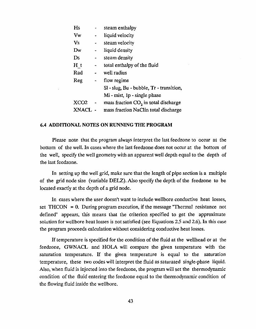
HsVwVs
Ow
Ds
Ht
Rad
Reg
XC02
XNACL -
steam enthalpy
liquid velocity
steam velocity
liquid density
steam density
total enthalpy of the fluid
well radius
flow regime
51 - slug, Bu - bubble, Tr - transition,
Mi - mist, Ip - single phasemass fraction CO2 in total discharge
mass fraction NaClin total discharge
6.4 ADDITIONAL NOTES ON RUNNING THE PROGRAM
Please note that the program always interpret the last feedzone to occur at the
bottom of the well. In cases where the last feedzone does not occur at the bottom of
the well, specify the well geometry with an apparent well depth equal to the depth of
the last feedzone.
In setting up the well grid, make sure that the length of pipe section is a multiple
of the grid node size (variable DELZ). Also specify the depth of the feedzone to be
located exactly at the depth of a grid node.
In cases where the user doesn't want to include wellbore conductive heat losses,
set THCON = O. During program execution, if the message "Thermal resistance not
defined" appears, this means that the criterion specified to get the approximatesolution for wellbore heat losses is not satisfied (see Equations 2.5 and 2.6). In this casethe program proceeds calculation without considering conductive heat losses.
If temperature is specified for the condition of the fluid at the wellhead or at thefeedzone, GWNACL and HOLA will compare the given temperature with the
saturation temperature. If the given temperature is equal to the saturation
temperature, these two codes will interpret the fluid as saturated single-phase liquid.
Also, when fluid is injected into the feedzone, the program will set the thermodynamic
condition of the fluid entering the feedzone equal to the thermodynamic condition of
the flowing fluid inside the wellbore.
43
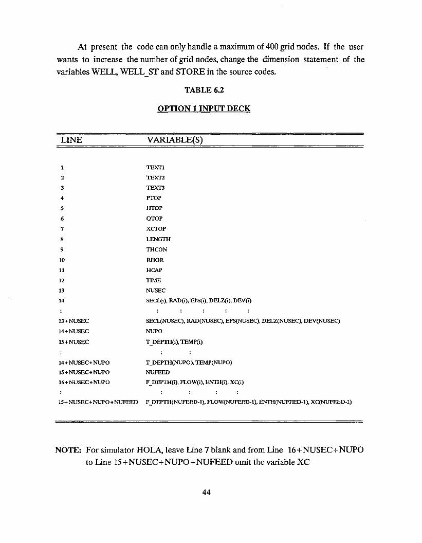
At present the code can only handle a maximum of 400 grid nodes. If the user
wants to increase the number of grid nodes, change the dimension statement of the
variables WELL, WELL_ST and STORE in the source codes.
TABLE 6.2
OPTION 1 INPUT DECK
LINE VARIABLE(S)
1 TEXTI
2 TEXT2
3 TEXT3
4 PTOP
5 HTOP
6 QTOP
7 XCTOP
8 LENGTII
9 TIICON
10 RHOR
11 HCAP
12 TIME
13 NUSEC
14 SECL(i). RAD(i). EPS(i). DELZ(i). DEV(i)
13 + NUSEC SECL(NUSEC), RAD(NUSEC), EPS(NUSEC), DELZ(NUSEC), DEV(NUSEC)
14+NUSEC NUPO
15+NUSEC T_DEPTH(i),1EMP(i)
14 + NUSEC+ NUPO T_DEPTII(NUPO), TEMP(NUPO)
15 + NUSEC+ NUPO NUFEED
16 + NUSEC +NUPO F_DEPTII(i). FLOW(i). ENTI:I(i), XC(i)
15+ NUSEC+ NUPO + NUFEED F_DEPTII(NUFEED-l), FLOW(NUFEED-l). ENIH(NUFEED-l). XC(NUFEED-l)
NOTE: For simulator HOLA, leave Line 7 blank and from Line 16+NUSEC+ NUPO
to Line lS+ NUSEC+NUPO+ NUFEED omit the variable XC
44
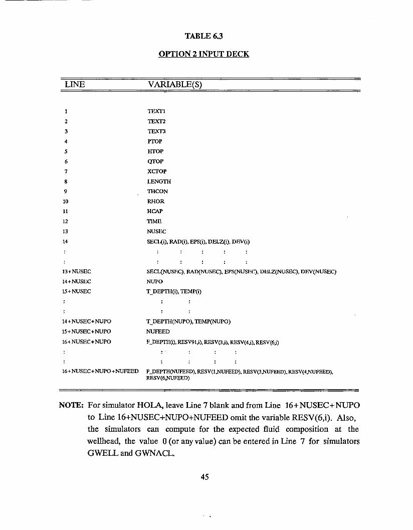
TABLE 6.3
OPTION 2 INPUT DECK
LINE VARlABLE(S)
1 lEXTl
2 lEXTl
3 TEXT3
4 PTOP
5 HTOP
6 QTOP
7 xcrop
8 LENGTIl
9 TIlCON
10 RHOR
11 HCAP
12 TIME
13 NUSEC
14 SECL(i), RAD(i), EPS(i), DELZ(i), DEV(i)
13+NUSEC
14+NUSEC
15+NUSEC
14 +NUSEC+ NUPO
15+ NUSEC + NUPO
16 +NUSEC + NUPO
SECL(NUSEq, RAD(NUSEq, EPS(NUSEq, DELZ(NUSEq, DEV(NUSEq
NUPO
T_DEPTIl(i), lEMP(i)
T_DEPTIl(NUPO), lEMP(NUPO)
NUFEED
F_DEPTH(i), RESV9l,i), RESV(3,i). RESV(4,i), RESV(6,i)
16+ NUSEC+ NUPO +NUFEED F_DEPTH(NUFEED), RESV(l,NUFEED). RESV(3,NUFEED), RESV(4,NUFEED).RESV(6,NUFEED)
NOTE: For simulatorHO~ leave Line 7 blank and from Line 16+ NUSEC+ NUPO
to Line 16+NUSEC+NUPO+NUFEED omit the variable RESV(6,i). Also,the simulators can compute for the expected fluid composition at the
wellhead, the value 0 (or any value) can be entered in Line 7 for simulators
GWELL and GWNACL.
45
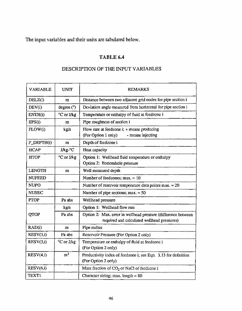
The input variables and their units are tabulated below.
TABLE 6.4
DESCRIPTION OF THE INPUT VARIABLES
VARIABLE UNIT REMARKS
DELZ(i) m Distance between two adjacent grid nodes for pipe section i
DEV(i) degree CO) Deviation angle measured from horizontal for pipe section i
ENTH(i) °C or J/kg Temperature or enthalpy of fluid at feedzone i
EPS(i) m Pipe roughness of section i
FLOW(i) kg/s Flow rate at feedzone i; + means producing(For Option 1 only) - means injecting
F_DEPTH(i) m Depth of feedzone i
HeAP J/kg_OC Heat capacity
HTOP °C or J/kg Option 1: Wellhead fluid temperature or enthalpy
Option 2: Bottomhole pressure
LENGTH m Well measured depth
NUFEED Number of feedzones; max. = 10
NUPO Number of reservoir temperature data points max. = 20
NUSEC Number of pipe sections; max. = 50
PTOP Paabs Wellhead pressure
kg/s Option 1: Wellhead flow rate
QTOP Paabs Option 2: Max. error in wellhead pressure (difference betweenrequired and calculated wellhead pressures)
RAD(i) m Pipe radius
RESV(l,i) Pa abs Reservoir Pressure (For Option 2 only)
RESV(3,i) °C or J/kg Temperature or enthalpy of fluid at feedzone i(For Option 2 only)
RESV(4,i) m3 Productivity index of feedzone i; see Eqn. 3.13 for definition(For Option 2 only)
RESV(6,i) Mass fraction of CO2 or NaO of feedzone i
TEXT1 Character string; max. length = 80
46
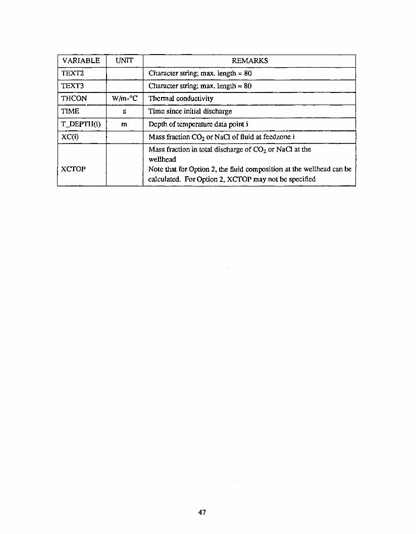
VARIABLE UNIT REMARKS
TEX12 Cnaracter string; max. length = 80
TEXT3 Character string; max. length = 80
THCON W/m_oC Thermal conductivity
TIME s Time since initial discharge
T_DEPTH(i) m Depth of temperature data point i
XC(i) Mass fraction CO2 or NaQ of fluid at feedzone i
Mass fraction in total discharge of CO2 or NaQ at the
wellheadXCTOP Note that for Option 2, the fluid composition at the wellhead can be
calculated. For Option 2, XCTOP may not be specified
47
REFERENCES
AhsanuIlah, AKM.; ''Temperature Variation of Surface Tension of Water." Proc.
Pakistan Acad. Sci., Vol. 9, No.2, pp. 97-108, 1972.
Ahsanullah, AKM.; 'Temperature Variation of Surface Tension of Water-NaCI
System, and Discussion of Origin of Discontinuity Observed in Pure Liquids and
Solutions." Proc. Pakistan Acad. Sci., Vol. 9, No.2, pp. 119-129, 1972.
Aunzo, Z.P.; "GWELL: A Multi-Component Multi-Feedzone Geothermal Wellbore
Simulator." M.S. Thesis, University of California at Berkeley, Berkeley, CA, USA,
May, 1990.
Barelli, A, Corsi, R., Del Pizzo, G. and Scali, C.; "A Two-Phase Flow Model for
Geothermal Wells in the Presence of Non-Condensible Gas." Geothermics, Vol.
11,~o.3,pp. 175-191, 1982.
Beggs, H.D.; "An Experimental Study of Two-Phase III Inclined Pipes." Ph.D.
Dissertation, University of Tulsa, Oklahoma, USA, 1972.
Bjornsson, G.; "A Multi-Feedzone Geothermal Wellbore Simulator." Earth Sciences
Division, Lawrence Berkeley Laboratory Report LBL-23546, Berkeley, CA, USA,
May 1987.
Bodvarsson, G.S., Pruess, K and Lippmann, M.J.; "Modelling of Geothermal Systems."
Journal of Petroleum Technology, September, 1986, pp. 1007-1021.
Buff, F.P. and Stillinger, F.R., Jr.; "Surface Tension of Ionic Solutions." The Jour. of
Chern. Phys., Vol. 25, No.2, pp. 312-318, 1956.
Burden, L.B., Faires, J.D. and Reynolds, AC.; "Numerical Analysis." 2nd Edition,
Prindle, Weber and Schimdt, Boston, USA, 1981.
Butler, J.N.; "Carbon Dioxide Equilibria and Their Applications." Addison-Wesley
Publishing Company, Inc., 1982.
48

Carslaw, H.S. and Jaeger, J.e.; "Conduction of Heat in Solids." Oxford University
Press, 2nd Editon, 1959.
Catigtig, D.e.; "Boreflow Simulation and Its Application to Geothermal Well Analysis
and Reservoir Assessment." UNU Geothermal Training Programme, Report No.
1983-8, Iceland, 1983.
Chisholm, D.; "Pressure Gradients due to Friction During the Flow of Evaporating
Two-Phase Mixtures in Smooth Tubes and Channels." Int. J. Heat Mass Transfer,
Vol. 16, pp. 347-358, 1973.
Conte, S.D. and De Boor, C.; "Elementary Numerical Analysis." McGraw-Hill Book
Company, 3M, 1980.
Dittman, G.L.; "Calculation of Brine Properties." Lawrence Livermore Laboratory
Report No. UCID-17406, Livermore, CA, USA, February, 1977.
Dittman, G.L.; "Wellflow for Geothermal Wells - Description of a Computer Program
Including the Effects of Brine Composition." Lawrence Livermore Laboratory
Report UCID-17473, Livermore, CA, May, 1977.
Dorn, W.S. and McCracken, D.D.; "Numerical Methods with FORTRAN IV Case
Studies." John Wiley ans Sons, Inc., 1972.
Ellis, AJ. and Golding, R.M.; "The Solubility of Carbon Dioxide Above 100°C in\Vater and in Sodium Chloride Solutions." American Journal of Science, Vol. 261,
pp. 47-60, January, 1963.
Engineering Science Data; 'The Gravitational Component of Pressure Gradient for
Two-Phase Gas or Vapour/Liquid Flow Thorugh Straight Pipes." Engineering
Science Data Item No. 77016, 1977.
Freeston, D.H. and Hadgu, T.; "Modelling of Geothermal Wells with Multiple Feed
Points: A Preliminary Study." Proc. 9th New Zealand Geothermal Workshop, 1987.
49
Gaulke, S.W.; "The Effect of CO2 on Reservoir Behavior for Geothermal Systems."
Earth Sciences Division, Lawrence Berkeley Laboratory Report LBlr22720,
Berkeley, CA, USA, December, 1986.
Gittens, G.J.; "Variation of Surface Tension of Water with Temperature." Journal of
Colloid and Interface Science, Vol. 30, No.3, pp. 406-412, July, 1969.
Gould, T.L.; "Vertical Two-Phase Steam-Water Flow in Geothermal Wells." Jour. Pet.
Tech., pp. 833-842, August, 1974.
Gould, T.L., Rasin Tek, M. and Katz, D.L.; 'Two-Phase Flow Through Vertical,
Inclined, or Curved Pipe." Jour. Pet. Tech., Vol. 257, pp. 915-926, August, 1974.
Haas, J.L. Jr.; "Physical Properties of the Coexisting Phase and THermophysical
Properties of the H 20 Component in Boiling NaCI Solutions." Preliminary Steam
Tables for Nacl Solutions, Geological Survey Bulletin 1421-A, United States
Government Printing Office, Washington, USA, 1976.
Hadgu, T., Freeston, D.H. and O'Sullivan, M.J.; "Studies of the Flow in the liner of a
Geothermal WelL" Trans. Geothermal Resources Council, Vol. 12, pp. 461-468,
October, 1988.
Haywood, R.W., Knights, G.A, Middleton, G.F. and Thorn, J.R.S.; "Experimental
Study of the Flow Conditions and Pressure Drop of Steam-Water Mixtures at High
Pressures in Heated and Unheated Tubes." Proc. Instn. Mech. Engrs., 175(13), pp.
669-726, 1961.
Heuer, GJ.; "Interfacial Tension of Water Against Hydrocarbon and Other Gases and
Adsorption of Methane on Solids at Reservoir Temperatures and Pressures." Ph.D.Dissertation, University of Texas, Austin, Texas, USA, June, 1957.
Horvath, AL.; "Handbook of Aqueous Electrolyte Solutions. Physical Properties,
Estimation and Correlation Methods." Ellis Horwood limited, England, 1985.
50
Hough, E.W., Heuer, GJ. and Walker, J.W.; "An Improved Pendant Drop, Interfacial
Tension Apparatus and Data for Carbon Dioxide and Water." Petroleum
Transactions, AIME, Vol. 216, pp. 469-472, 1959.
Jho, c., Nealon, D., Shogbola, S. and King, AD., Jr.; "Effect of Pressure on the Surface
Tension of Water: Adsorption of Hydrocarbon Gases and Carbon Dioxide on
Water at Temperatures Between 0 and 50°C." Journal of Colloid and Interface
Science, Vol. 65, No.1, pp. 141-154, June, 1978.
Kestin, J., Sengers, J.V., Parsi-Kamgar, B. and Levelt Sengers, J.M.H.;
"Thermophysical Properties of Fluid H20." J. Phys. Chern. Ref. Data, Vol. 13, No.
1, pp. 175-183, 1984.
Lombardi, C. and Ceresa, I.; "A Generalized Pressure Drop Correlation in Two-Phase
Flow. "Energia NUcleare, Vol. 25, No.4, pp. 181-198, April, 1978.
Martinelly, R.C. and Nelson, D.B.; "Prediction of Pressure Drop During ForcedCirculation of Boiling Water." Trans. Amer. Soc. Mech. Engrs., 70(6), pp. 695-702,
1948.
Miller, C.W.; "Welbore User's ManuaL" Earth Sciences Division, Lawrence Berkeley
Laboratory Report No. LBL-1091O, Berkeley, CA, January, 1980.
Mukherjee, H.; "An Experimental Study of Inclined Two-Phase Flow." Ph.D.
Dissertation, University of Tulsa, Oklahoma, USA, 1979.
Orkiszewski, J.; "Predicting Two-Phase Pressure Drop in Vertical Pipes." Jour. Pet.Tech., pp. 829-838, June, 1967.
Parlactuna, M.; "Two-Phase Wellbore Simulator and Analysis of Reinjection Data
from Svartsengi, Iceland." The UNU Geothermal Training Programme, Iceland,
Report No. 1985-7, 1985.
51

Phillips, S.L., Igbene, A, Fair, I.A, Ozbek, H. and Tavan~ M.; "A Technical Databook
for Geothermal Energy Utilization." Lawrence Berkeley Laboratory Report No.
LBL-12810, Berkeley, CA, USA, June, 1981.
Phillips, S.L., Ozbek, H. and Silvester, L.F.; "Density of Sodium Chloride Solutions at
High Temperatures and Pressures." Lawrence Berkeley Laboratory Report LEI.,..
16275, Berkeley, CA, USA, June, 1983.
Pitzer, KS.; 'The Thermodynamics of Sodium Chloride Solutions in Steam." Lawrence
Berkeley Laboratory Report LBL-14886, Berkeley, CA, USA, August, 1982.
Pitzer, K.S.; 'Thermodynamic Properties of Aqueous NaCI from 273 to 823 OK with
Estimates for Higher Temperatures." Lawrence Berkeley Laboratory Report LBL
18183, Berkeley, CA, USA, July, 1984.
Potter, R.W. II and Brown, D.L.; "The Volumetric Properties of Aqueous Sodium
Chloride Solutions from 0° to 500°C at Pressures up to 2000 Bars Based on a
Regression of Available Data in the Literature." Preliminary Steam Tables for
NaCI Solutions, Geological Survey Bulletin 1421-C, United States Government
Printing Office, Washington, 1976.
Pritchett, J.W., Rice, M.H. and Riney, T.D.; "Equation-of-State for Water-Carbon
Dioxide Mixtures: Implications for Baca Reservoir." DOE/ET/27163-8, 1981.
Pruess, K; "TOUGH User's Guide." Lawrence Berkeley Laboratory Report LBL
20700, Berkeley, CA, USA, April, 1986.
Sourirajan, S. and Kennedy, G.C.; 'The System H 20-NaCI at Elevated Temperatures
and Pressures." Amer. Jour. of Science, Vol. 260, pp. 115-141, February, 1962.
Sutton, F.M.; "Pressure-Temperature Curves for a Two-Phase Mixture of Water and
Carbon Dioxide." New Zealand Journal of Science, Vol. 19, pp. 297-301, 1976.
Sutton, F.M. and McNabb, A; "Boiling Curves at Broadlands Geothermal Field, New
Zealand." New Zealand Journal of Science, Vol. 20, pp. 333-337, 1976.
52
Sweigert, R.L., Wever, P. and Allen, R.L.; ''Thermophysical Properties of Gases.
Carbon Dioxide." Industrial and Engineerign Chemistry, 38, (2), pp.185-200, 1946.
Takenouchi, S. and Kennedy, G.e.; ''The Binary System ~0-C02 at High
Temperatures and Pressures." Am. J. Sci., Vol. 262, p. 1055, 1964.
Unterberg, W.; ''Thermophysical Properties of Aqueous Sodium Chloride Solutions."
UCLA Department of Engineering Report No. 64-21, Los Angeles, CA, USA,
May, 1964.
Upadhay, R.N., Hartz, J.D., Tomkoria, B.N. and Gulati, M.S.; "Comparison of
Calculated and Observed Pressure Drops in Geothermal Wells Producing Steam
Water Mixtures." Proc. 520d Annual Fall Technical Conference and Exhibition of
the Soc. of Pet. Engrs. of AIME, Denver, Colorado, USA, SPE-6766, 1977.
Vargaftik, N.B., Volkov, B.N. and Voljak, L.D.; "International Tables of the Surface
Tension of Water." J. Phys. Chern. Ref. Data, Vol. 12, No.3, pp. 817-820, 1983.
Vukalovich, M.P. and Altunin, V.V.; "Thermophysical Properties of Carbon Dioxide."
Collet's (Publisher) Ltd., London and Wellingborough, 1968.
Wahl, E.F.; "Geothermal Energy Utilization." John Wiley and Sons, Inc., pp. 60-63,
1977.
Wallis, G.B.; "One-Dimensional Two-Phase Flow." McGraw-Hill, USA, 1969.
Weres, 0., Peiper, J.e. and Pitzer, KS.; "Documentation for Computer Code NaCl."
Lawrence Berkeley Laboratory Report No. LBL-21859, Berkeley, CA, USA,February, 1987.
White, F.M.; "Fluid Mechanics." McGraw-Hill, USA, 1979.
53

FIGURES
54
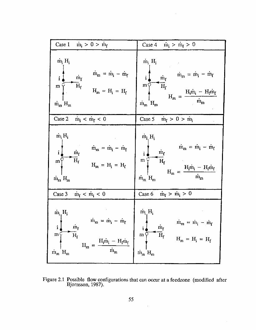
Case 1 Case 4 ffii > mr > 0
m = m· - mrm 1
m· H·JI mt..
Case 2 mi < me < 0 Case 5 mr > 0 > mi
Case 3me < ~ < 0 Case 6 me > mi > 0
Figure 2.1 Possible flow configurations that can occur at a feedzone (modified afterBjornsson, 1987).
55

r:- .0 \)
0 00
' ..
0 & j j l ..
0 0 I I . l0 0
tI 0
0 ( ~ .. '~
0 .. , 00
.. , ..0 l..L .. l..L
0 '+- -0 0 0
0· ..
c c r . .\)
00 0
0 ...... ...... Ir:..
0 00 Q) Q)
0 L.-L.-
0 0 0 . ..0 ~ · ..0 0
....,.- ·,.l- --
Bubble Slug Annular-Slug Annular-MistTransition
Figure 4.1 Illustration of the different flow regimes (after Orkiszewski, 1967).
56
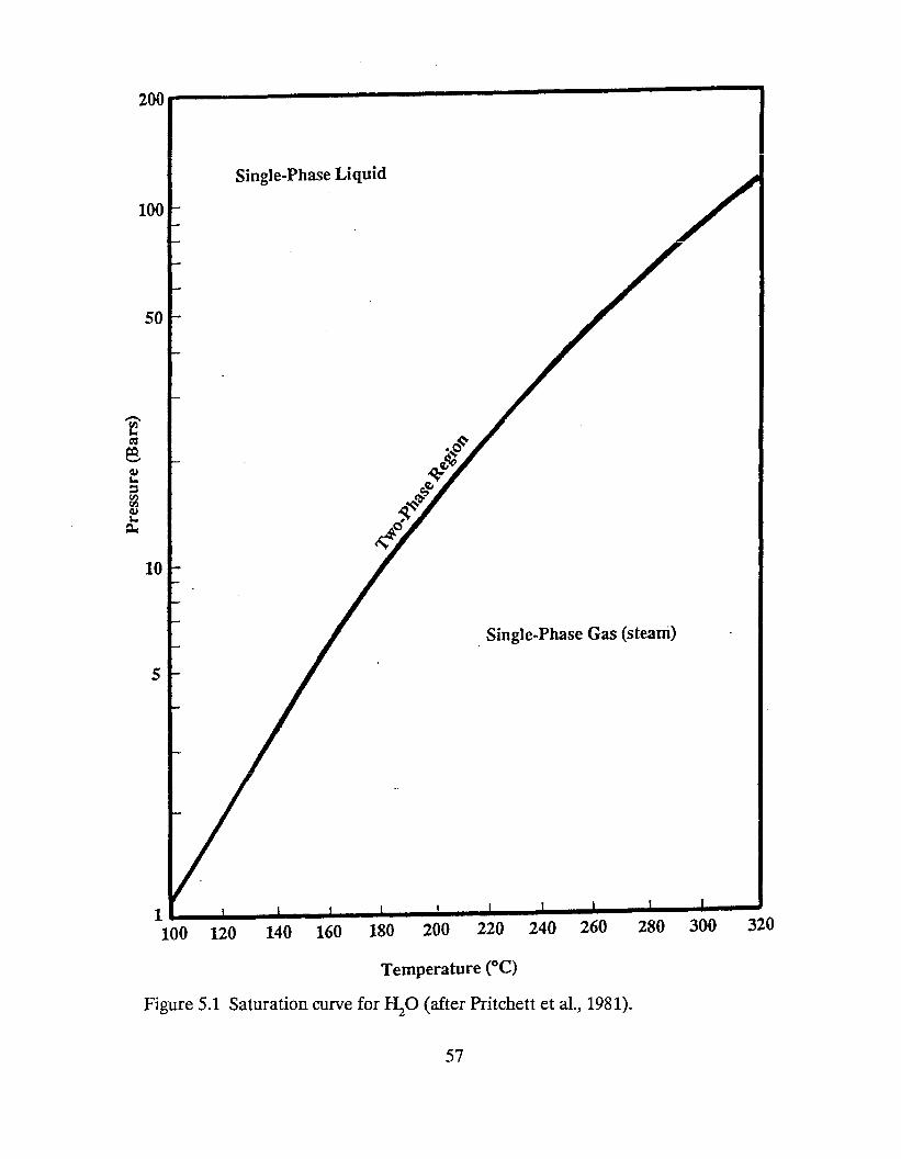
Single-Phase Liquid
100
50
10
5
Single-Phase Gas (steam)
I
lL-_I...-_..-._.....-.l~_...._"---"--......I_-,&,..,.----.J100 120 140 160 180 200 220 240 260 280 300 320
Temperature (OC)
Figure 5.1 Saturation curve for ~O (after Pritchett et aI., 1981).
57

200 .....----------------------.,
100
50
Single-Phase Liquid
Single-Phase Gas (steam, CO~
1...._1.-_""--_..L-._""--_-'-_.... ......- .....- ......-..J
100 120 140 160 180 200 220 240 260 280 300 320
Temperature (OC)
Figure 5.2 Saturation curve for H20-C02 system with 1% CO2 (after Pritchett et aI.,1981).
58
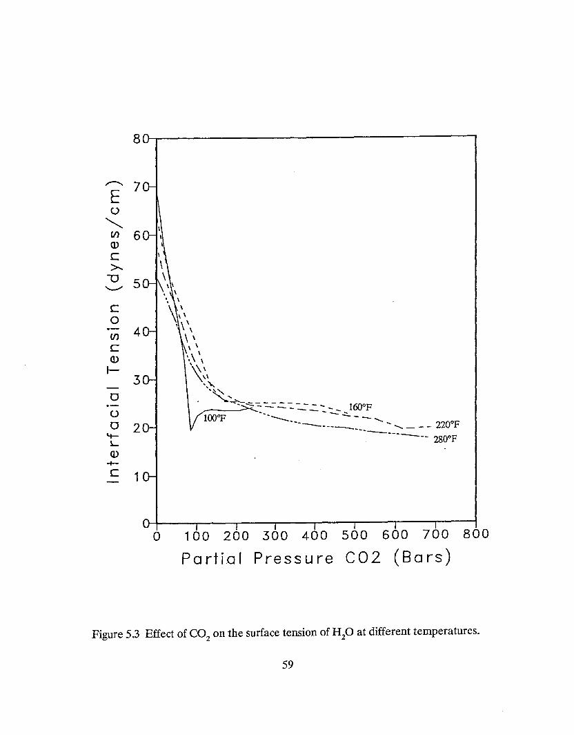
..--....E()
"'-(/) 6Q)
c>..
"'0 5'--"
c0
(/) 4cQ)
t-3
0.-()
0 2'+-LQ)
-+-c 1
a 100 200 300 400 500
Partial Pressure C02
600 700
(B a rs)
800
Figure 5.3 Effect of CO2
on the surface tension of H20 at different temperatures.
59
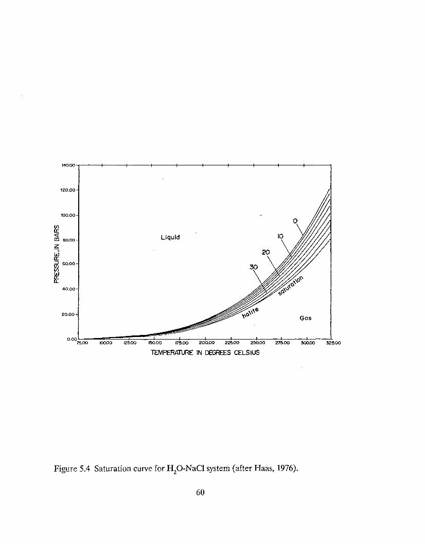
140.00.,----f----t-----t-----ir----t----t----f-----<t-----t-------,
'20.00
'00.00
Cf)0::<I:C!) BO.oO
~
W0::m60.00
~40.00
20.00
liquid
o.ooL---==~~~~___4______+_~75.00 100.00 125.00 150.00 175.00 200.00 225.00 250.00 275.00 300.00 325.00
TEMPERAnRE IN DEGREES CELSIUS
Figure 5.4 Saturation curve for H20-NaCI system (after Haas, 1976).
60
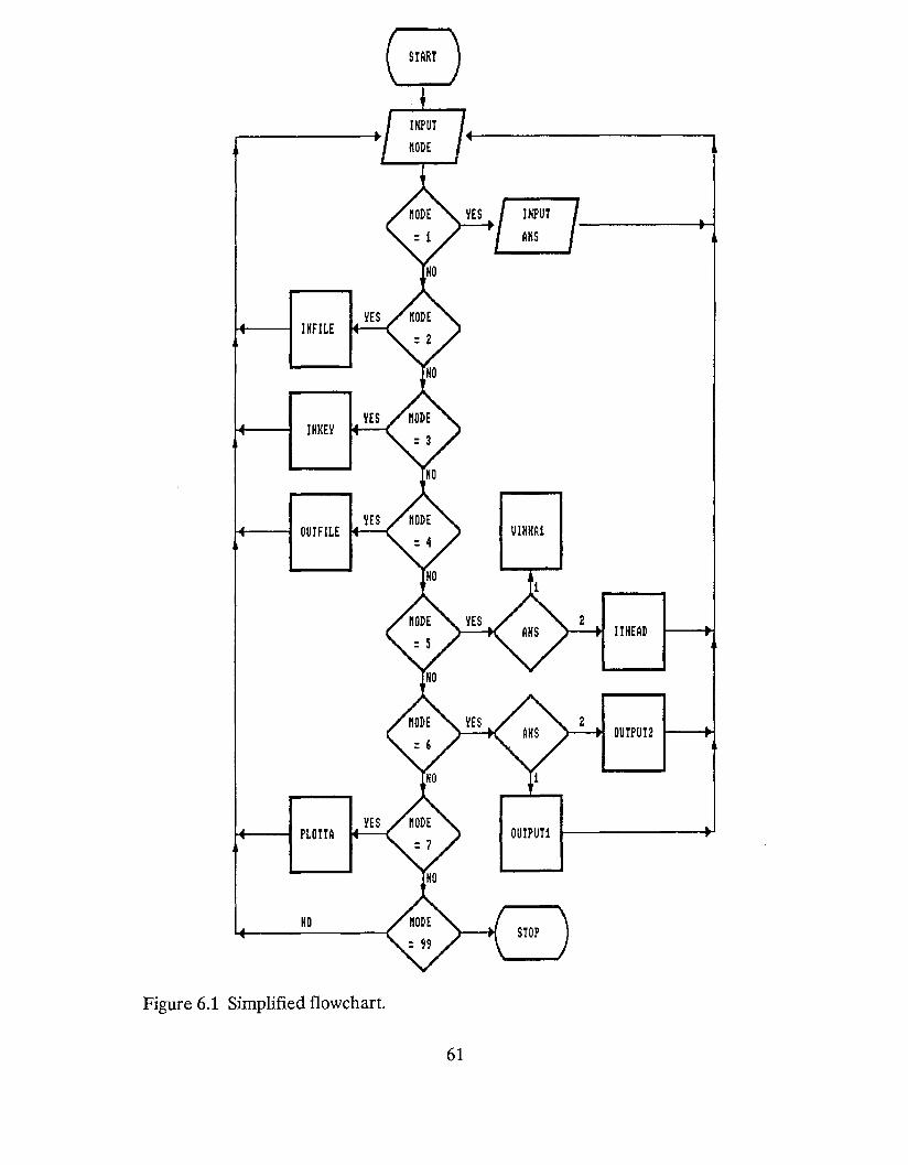
INFILE
INI<EY
I-f---l OUIFILE
I-f---l PLOm
NO
Figure 6.1 Simplified flowchart.
61
YES ~-----~H~
UINNA1
IIHEAD
OUIPUI2 1---+1
OUIPUI1 1---------+1
APPENDIX A
(SAMPLE RUNS FOR GWELL)
62

SAMPLE 1 INPUT FILE
fluid at the wellhead -
90.088.086.084.082.080.078.076.074.072.070.068.066.064.062.060.060.060.060.060.0
25.015.015.015.015.015.015.015.015.015.015.015.015.015.015.015.025.010.025.020.0
4.6E-54.6E-54.6E-54.6E-54.6E-54.6E-54.6E-54.6E-54.6E-54.6E-54.6E-54.6E-54.6E-54.6E-54.6E-54.6E-54.6E-54.6E-51. 5E-51. 5E-5
0.11020.11020.11020.11020.11020.11020.11020.11020.11020.11020.11020.11020.11020.11020.11020.11020.11020.11020.08730.0873
Sample 1 for simulator GWELL- option 1 used-- The well is producing two-phase
0.7000E+06161.0100.00000.032530.0000.0002800.0001000.0006.0480E+0520
300.030.030.030.030.030.030.030.030.030.030.030.030.030.030.030.0
150.010.0
1600.020.0
40.0
1000.02000.02500.0
31110.01810.0
25.00260.00310.00330.00
20.0040.00
1.7000E+061.2000E+06
0.100.02
SAMPLE 1 GWELL.LOG FILE
Two phase to water phaseTemperature X2 Depth
0.271164E+03 -0.00095425 1310.0
63
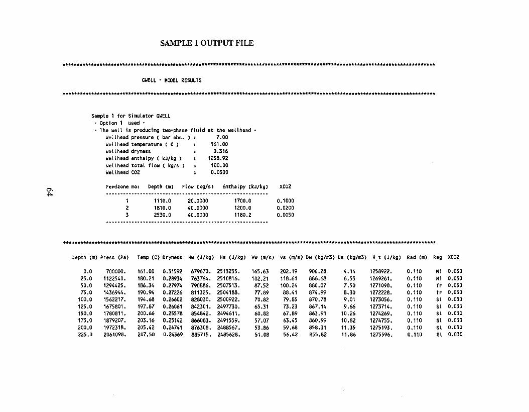
SAMPLE 1 OUTPUT FILE
***w******************************************************************************************************************************
GWELL - MODEL RESULTS
**********************************************************************************************************************************
Sample 1 for Simulator GWELL
the wellhead·7.00
161.000.316
1258.92100.000.0300
Option 1 used-The well is producing two-phase fluid at
We~lhead pressure ( bar abs. )Wellhead temperature ( C )Wellhead drynessWellhead enthalpy ( kJ/kg )Wellhead total flow ( kg/s )Wellhead C02
FeP.dzone no: Depth (m) Flow (kg/s) Enthalpy (kJ/kg)0\~
123
1110.01810.02530.0
20.000040.000040.0000
1700.01200.01180.2
XC02
0.10000.02000.0050
**********************************************************************************************************************************
Depth (m) Press ePa) Temp (C) Dryness Hw (J/kg) Hs (J/kg) Vw em/s) Vs (m/s) Ow (kg/m3) Os (kg/m3) H_t (J/kg) Rad em) Reg XC02
0.0 700000. 161.00 0.31592 679670. 2513235. 165.63 202.19 906.28 4.14 1258922. 0.110 Hi 0.03025.0 1122540. 180.21 0.28934 763764. 2510816. 102.21 118.61 886.68 6.53 1269261- 0.110 Hi 0.03050.0 1294425. 186.34 0.27974 790886. 2507513. 87.52 100.24 880.07 7.50 1271090. 0.110 Tr 0.03075.0 1436944. 190.94 0.27226 811325. 2504188. 77.89 88.41 874.99 8.30 1272228. 0.110 Tr 0.030
100.0 1562217. 194.68 0.26602 828030. 2500922. 70.82 79.85 870.78 9.01 1273056. 0.110 Sl 0.030125.0 1675801. 197.87 0.26061 842301. 249mO. 65.31 73.23 867.14 9.66 1273714. 0.110 Sl 0.030150.0 1780811. 200.66 0.25578 854842. 2494611. 60.82 67.89 863.91 10.26 1274269. 0.110 Sl 0.030175.0 1879207. 203.16 0.25142 866083. 2491559. 57.07 63.45 860.99 10.82 1274755. 0.110 Sl 0.030200.0 1972318. 205.42 0.24741 876308. 2488567. 53.86 59.68 858.31 11.35 1275193. 0.110 Sl 0.030225.0 2061098. 207.50 0.24369 885715. 2485628. 51.08 56.42 855.82 11.86 1275596. 0.110 Sl 0.030
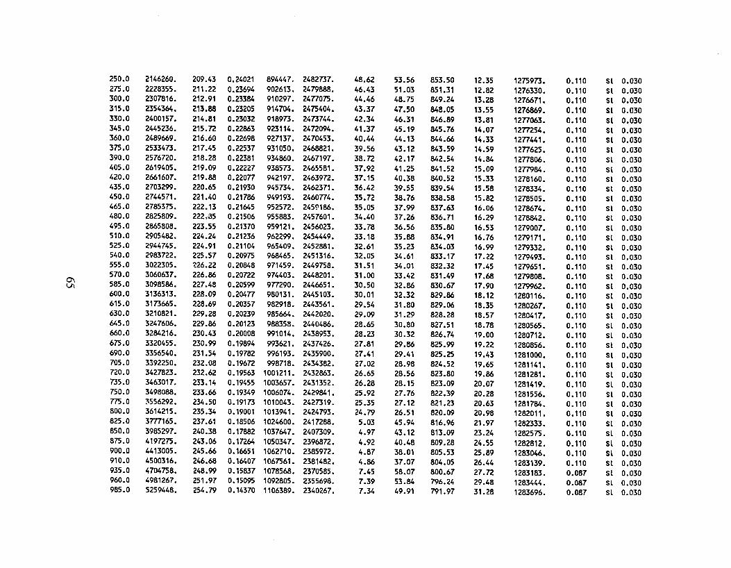
250.0 2146260. 209.43 0.24021 894447. 2482737. 48.62 53.56 853.50 12.35 1275973. 0.110 Sl 0.030275.0 2228355. 211.22 0.23694 902613. 2479888. 46.43 51.03 851.31 12.82 1276330. 0.110 Sl 0.030300.0 2307816. 212.91 0.23384 910297. 24n075. 44.46 48.75 849.24 13.28 1276671. 0.110 Sl 0.030315.0 2354364. 213.88 0.23205 914704. 2475404. 43.37 47.50 848.05 13.55 1276869. 0.110 Sl 0.030330.0 2400157. 214.81 0.23032 918973. 2473744. 42.34 46.31 846.89 13.81 12n063. 0.110 Sl 0.030345.0 2445236. 215.n 0.22863 923114. 2472094. 41.37 45.19 845.76 14.07 12m54. 0.110 Sl 0.030360.0 2489669. 216.60 0.22698 927137. 2470453. 40.44 44.13 844.66 14.33 12n441. 0.110 Sl 0.030375.0 2533473. 217.45 0.22537 931050. 2468821. 39.56 43.12 843.59 14.59 12n625. 0.110 Sl 0.030390.0 2576720. 218.28 0.22381 934860. 2467197. 38.72 42.17 842.54 14.84 12n806. 0.110 Sl 0.030405.0 2619405. 219.09 0.22227 938573. 2465581. 37.92 41.25 841.52 15.09 1277984. 0.110 Sl 0.030420.0 2661607. 219.88 0.220n 942197. 2463972. 37.15 40.38 840.52 15.33 1278160. 0.110 Sl 0.030435.0 2703299. 220.65 0.21930 945734. 2462371. 36.42 39.55 839.54 15.58 1278334. 0.110 Sl 0.030450.0 2744571. 221.40 0.21786 949193. 2460n4. 35.72 38.76 838.58 15.82 1278505. 0.110 Sl 0.030465.0 2785375. 222.13 0.21645 952572. 2459186. 35.05 37.99 837.63 16.06 1278674. 0.110 Sl 0.030480.0 2825809. 222,35 0.21506 955883. 2457601. 34.40 37.26 836.71 16.29 1278842. 0.110 Sl 0.030495.0 2865808. 223.55 0.21370 959121. 2456023. 33.78 36.56 835.80 16.53 1279007. 0.110 Sl 0.030510.0 2905482. 224.24 0.21236 962299. 2454449. 33.18 35.88 834.91 16.76 1279171. 0.110 Sl 0.030525.0 2944745. 224.91 0.21'104 965409. 2452881. 32.61 35.23 834.03 16.99 1279332. 0.110 Sl 0.030540.0 2983722. 225.57 0.20975 968465. 2451316. 32.05 34.61 833.17 17.22 1279493. 0.1'10 Sl 0.030555.0 3022305. ~26.22 0.20848 971459. 2449758. 31.51 34.01 832.32 17.45 1279651. 0.110 Sl 0.030570.0 3060637. 226.86 0.20722 974403. 2448201. 31.00 33.42 831.49 17.68 1279808. 0.110 Sl 0.0300\ 585.0 3098586. 227.48 0.20599 9m90. 2446651. 30.50 32.86 830.67 17.90 1279962. 0.110 Sl 0.030VI600.0 3136313. 228.09 0.20/,n 980131. 2445103. 30.01 32.32 829.86 18.12 1280116. 0.110 Sl 0.030615.0 3173665. 228.69 0.20357 982918. 2443561. 29.54 31.80 829.06 18.35 1280267. 0.110 Sl 0.030630.0 3210821. 229.28 0.20239 985664. 2442020. 29.09 31.29 828.28 18.57 1280417. 0.110 Sl 0.030645.0 3247606. 229.86 0.20123 988358. 2440486. 28.65 30.80 827.51 18.78 1280565. 0.110 Sl 0.030660.0 3284216. 230.43 0.20008 991014. 2438953. 28.23 30.32 826.74 19.00 1280712. 0.110 Sl 0.030675.0 3320455. 230.99 0.19694 993621. 2437426. 27.81 29.86 825.99 19.22 1280856. 0.1'10 Sl 0.030690.0 3356540. 231.54 0.19782 996193. 2435900. 27.41 29.41 825.25 19.43 1281000. 0.110 Sl 0.030705.0 3392250. 232.08 0.196n 998718. 2434382. 27.02 28.98 824.52 19.65 1281141. 0.110 Sl 0.030720.0 3427823. 232.62 0.19563 1001211. 2432863. 26.65 28.56 823.80 19.86 1281281. 0.110 Sl 0.030735.0 3463017. 233.14 0.19455 1003657. 2431352. 26.28 28.15 823.09 20.07 1281419. 0.110 Sl 0.030750.0 3498088. 233.66 0.19349 1006074. 2429841. 25.92 27.76 822.39 20.28 1281556. 0.110 Sl 0.030775.0 ~556292. 234.50 0.19173 1010043. 2427319. 25.35 27.12 821.23 20.63 1281784. 0.110 Sl 0.030800.0 3614215. 235.34 0.19001 1013941. 2424793. 24.79 26.51 820.09 20.98 1282011. 0.110 Sl 0.030825.0 3m165. 237.61 0.18506 1024600. 2417288. 5.03 45.94 816.96 21.97 1282333. 0.110 Sl 0.030850.0 3985297. 240.38 0.17882 1037647. 2407309. 4.97 43.12 813.09 23.24 1282575. 0.110 Sl 0.030875.0 4197275. 243.06 0.17264 1050347. 23968n. 4.92 40.48 809.28 24.55 1282812. 0.110 Sl 0.030900.0 4413005. 245.66 0.16651 1062710. 2385972. 4.87 38.01 805.53 25.89 1283046. 0.110 Sl 0.030910.0 4500316. 246.68 0.16407 1067561. 2381482. 4.86 37.07 804.05 26.44 1283139. 0.110 Sl 0.030935.0 4704758. 248.99 0.15837 1078568. 2370585. 7.45 58.07 800.67 27.72 1283183. 0.087 Sl 0.030960.0 4981267. 251.97 0.15095 1092805. 2355698. 7.39 53.84 796.24 29.48 1283444. 0.087 Sl 0.030985.0 5259448. 254.79 0.14370 1106389. 2340267. 7.34 49.91 791.97 31.28 1283696. 0.087 Sl 0.030

1010.0 5538785. 257.48 0.13661 1119334. 2324320. 7.30 46.24 787.85 33.10 1283942. 0.087 Sl 0.0301035.0 5818600. 260.02 0.12968 1131648. 2307896. 7.27 42.81 783.89 34.95 1284182. 0.087 Sl 0.0301060.0 6098097. 262.43 0.12293 1143332. 2291049. 7.25 39.59 780.08 36.81 1284416. 0.087 Sl 0.0301085.0 6376409. 264.70 0.11636 1154388. 2273842. 7.24 36.58 n6.44 38.70 1284647. 0.087 Sl 0.0301110.0 6652647. 266.84 0.10999 1164817. 2256346. 7.23 33.78 m.97 40.59 1284875. 0.087 Sl 0.0301110.0 6652647. 265.68 0.02108 1158718. 2220567. 5.45 7.62 n4.85 41.06 1181106. 0.087 Sl 0.0131135.0 6831288. 266.59 0.01n6 1162962. 2196839. 5.33 6.84 m.37 42.47 1181319. 0.087 Sl 0.0131160.0 7004521. 267.41 0.01466 1166m. 2173505. 5.21 6.18 n2.03 43.86 1181533. 0.087 Sl 0.0131185.0 7173127. 268.16 0.01176 1170218. 2150549. 5.07 5.61 nO.80 45.22 1181746. 0.087 Sl 0.0131210.0 7338836. 268.85 0.00902 1173350. 2127803. 4.92 5.18 769.67 46.58 1181959. 0.087 Bu 0.0131235.0 7503628. 269.48 0.00640 1176231. 2105048. 4.76 4.83 768.61 47.95 1182172. 0.087 Bu 0.0131260.0 7668261. 270.08 0.00387 1178887. 2082231. 4.60 4.51 767.63 49.34 1182385. 0.087 Bu 0.0131285.0 '('832916. 270.63 0.00144 1181334. 2059375. 4.45 4.23 766.70 50.73 1182598. 0.087 Bu 0.0131310.0 8086022. 271.16 0.00000 1182812. O. 4.34 0.00 769.46 0.00 1182812. 0.087 1p 0.0131335.0 8261922. 271.22 0.00000 1183025. O. 4.34 0.00 769.62 0.00 1183025. 0.087 1p 0.0131360.0 8437853. 271.27 0.00000 1183237. O. 4.34 0.00 769.78 0.00 1183237. 0.087 1p 0.0131385.0 8613815. 271.32 0.00000 1183450. O. 4.34 0.00 769.94 0.00 1183450. 0.087 1p 0.0131410.0 8789808. 271.38 0.00000 1183662. O. 4.34 0.00 nO.10 0.00 1183662. 0.087 1p 0.0131435.0 8965833. 271.43 0.00000 1183875. O. 4.34 0.00 nO.25 0.00 1183875. 0.087 1p 0.0131460.0 9141888. 271.48 0.00000 1184087. o. 4.34 0.00 nO.41 0.00 1184087. 0.087 1p 0.0131485.0 9317975. 271.54 0.00000 1184300. O. 4.34 0.00 nO.57 0.00 1184300. 0.087 1p 0.0130\ 1510.0 9494092. 271.59 0.00000 1184512. O. 4.34 0.00 nO.73 0.00 1184512. 0.087 1p 0.0130\1535.0 9670241. 271.64 0.00000 1184725. O. 4.33 0.00 nO.88 0.00 1184725. 0.087 1p 0.01315,s0.0 9846420. 271.70 0.00000 1184937. O. 4.33 0.00 n1.04 0.00 1184937. 0.087 1p 0.0131585.0 10022630. 271.75 0.00000 1185150. O. 4.33 0.00 n1.20 0.00 1185150. 0.087 1p 0.0131610.0 11)198871. 271.80 0.00000 1185362. O. 4.33 0.00 n1.35 0.00 1185362. 0.087 1p 0.0131635.0 11375143. 271.86 0.00000 1185575 • O. 4.33 0.00 n1.51 0.00 1185575. 0.087 1p 0.0131660.0 10551445. 271.91 0.00000 1185787. O. 4.33 0.00 n1.67 0.00 1185787. 0.087 1p 0.0131685.0 1072m8. 271.96 0.00000 1186000. O. 4.33 0.00 n1.82 0.00 1186000. 0.087 1p 0.01317~0.0 10904142. 272.02 0.00000 1186212. O. 4.33 0.00 n1.98 0.00 1186212. 0.087 1p 0.0131735.0 11080536. 272.07 0.00000 1186425. O. 4.33 0.00 n2.13 0.00 1186425. 0.087 lp 0.0131760.0 11256960. 272.12 0.00000 1186637. o. 4.33 0.00 n2.29 0.00 1186637. 0.087 1p 0.0131785.0 11433415. 272.17 0.00000 1186850. O. 4.33 0.00 n2.44 0.00 1186850. 0.087 lp 0.0131810.0 11609900. 272.23 0.00000 1187062. O. 4.32 0.00 n2.59 0.00 1187062. 0.087 lp 0.0131810.0 11609900. 268.74 0.00000 1174129. O. 2.15 0.00 n8.48 0.00 1174129. 0.087 1p 0.0051835.0 l1n8418. 268.79 0.00000 1174341. o. 2.15 0.00 n8.62 0.00 1174341. 0.087 lp 0.0051860.0 11946966. 268.84 0.00000 1174554. o. 2.15 0.00 n8.76 0.00 1174554. 0.087 lp 0.0051885.0 12115542. 268.89 0.00000 1174766. O. 2.14 0.00 n8.90 0.00 1174766. 0.087 1p 0.0051910.0 12284147. 268.94 0.00000 1174979. O. 2.14 0.00 n9.04 0.00 1174979. 0.087 lp 0.0051935.0 12452782. 268.99 0.00000 1175191. o. 2.14 0.00 n9.18 0.00 1175191. 0.087 1p 0.0051960.0 12621445. 269.04 0.00000 1175404. O. 2.14 0.00 779.32 0.00 1175404. 0.087 lp 0.0051985.0 12790138. 269.09 0.00000 1175616. O. 2.14 0.00 n9.46 0.00 1175616. 0.087 lp 0.0052010.0 12958859. 269.14 0.00000 1175829. O. 2.14 0.00 n9.60 0.00 1175829. 0.087 1p 0.0052035.0 13127610. 269.19 0.00000 1176041. O. 2.14 0.00 n9.74 0.00 1176041. 0.087 1p 0.005
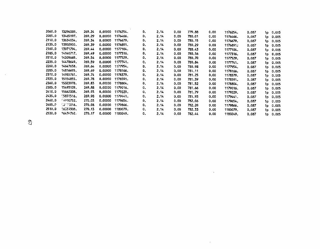
2060.0 13296389. 269.24 0.00000 1176254. o. 2.14 0.00 779.88 0.00 1176254. 0.087 1p 0.0052085.0 13465197. 269.29 0.00000 1176466. O. 2.14 0.00 780.01 0.00 1176466. 0.087 1p 0.0052110.0 13634034. 269.34 0.00000 1176679. O. 2.14 0.00 780.15 0.00 1176679. 0.087 1p 0.0052135.0 13802900. 269.39 0.00000 1176891. O. 2.14 0.00 780.29 0.00 1176891 : 0.087 1p 0.0052160.0 13971794. 269.44 0.00000 1177104. O. 2.14 0.00 780.43 0.00 1177104. 0.087 1p 0.0052185.0 14140717. 269.49 0.00000 11m16. O. 2.14 0.00 780.56 0.00 11m16. 0.087 1p 0.0052210.0 14309669. 269.54 0.00000 1177529. O. 2.14 0.00 780.70 0.00 1177529. 0.087 1p 0.0052235.0 14478649. 269.59 0.00000 11m41. O. 2.14 0.00 780.84 0.00 11m41. 0.087 1p 0.0052260.0 14647658. 269.64 0.00000 1177954. O. 2.14 0.00 780.98 0.00 1177954. 0.087 1p 0.0052285.0 14816695. 269.69 0.00000 1178166. O. 2.14 0.00 781.11 0.00 1178166. 0.087 1p 0.0052310.0 14985761. 269.74 0.00000 1178379. O. 2.14 0.00 781.25 0.00 1178379. 0.087 1p 0.0052335.0 15154855. 269.78 0.00000 1178591. O. 2.14 0.00 781.39 0.00 1178591. 0.087 1p 0.0052360.0 15323978. 269.83 0.00000 1178804. O. 2.14 0.00 781.52 0.00 1178804. 0.087 1p 0.0052385.0 15493129. 269.88 0.00000 1179016. O. 2.14 0.00 781.66 0.00 1179016. 0.087 1p 0.0052410.0 15662308. 269.93 0.00000 1179229. O. 2.14 0.00 781.79 0.00 1179229. 0.087 1p 0.0052435.0 ~5831516. 269.9& 0.00000 1179441. O. 2.14 0.00 781.93 0.00 1179441. 0.087 1p 0.0052460.0 "(,1,11)0752. 270.03 0.00000 1179654. O. 2.14 0.00 782.06 0.00 1179654. 0.087 1p 0.0052485.(\ '::l" ~'':I016. 270.08 0.00000 1179866. O. 2.14 0.00 782.20 0.00 1179866. 0.087 1p 0.0052510.0 ~6:i3i30B. 270.13 0.00000 1180079. O. 2.14 0.00 782.33 0.00 1180079. 0.087 1p 0.0052530.0 ~647t.762" 270.17 0.00000 1180249. O. 2.14 0.00 782.44 0.00 1180249. 0.087 1p 0.005
0\-....)
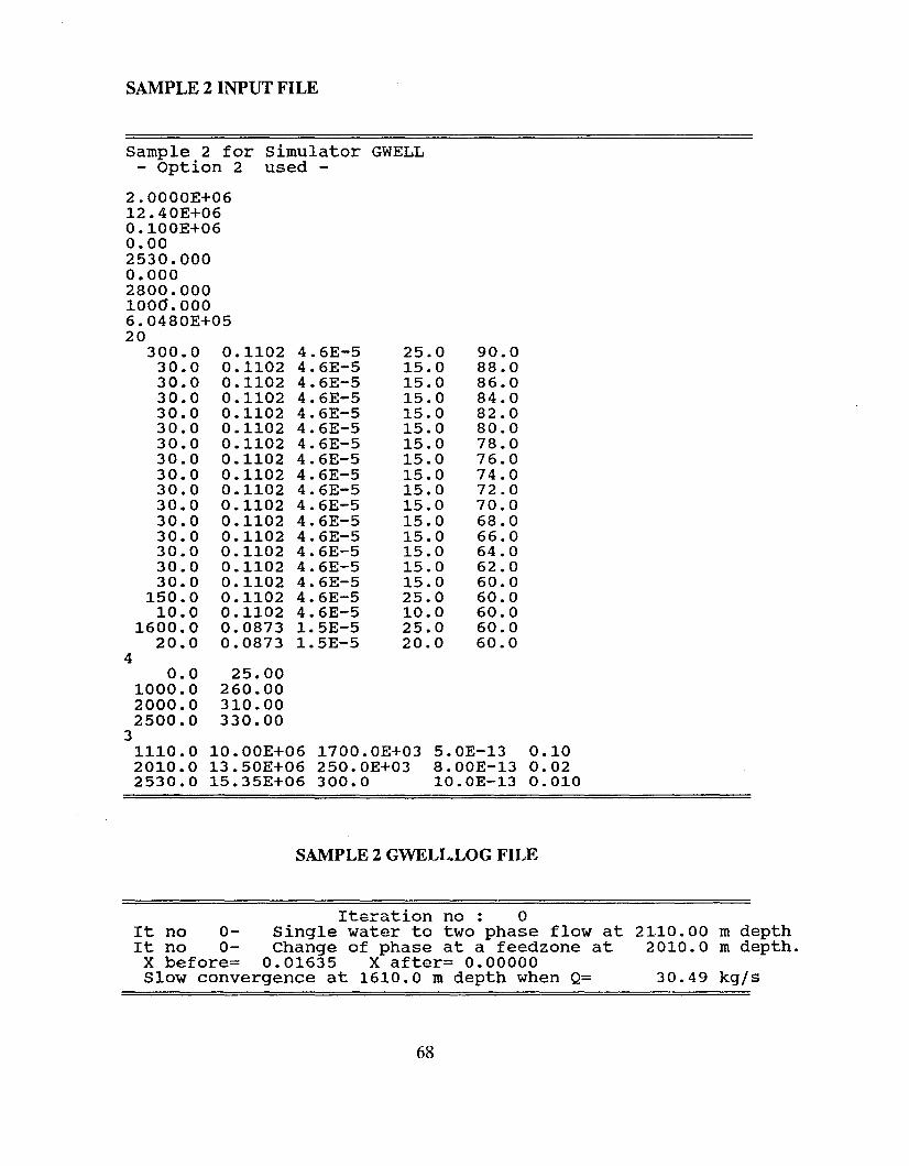
SAMPLE 2 INPUT FILE
Sample 2 for Simulator GWELL- option 2 used -
2.0000E+0612.40E+060.100E+060.002530.0000.0002800.000100d.0006.0480E+0520
300.0 0.1102 4.6E-5 25.0 90.030.0 0.1102 4.6E-5 15.0 88.030.0 0.1102 4.6E-5 15.0 86.030.0 0.1102 4.6E-5 15.0 84.030.0 0.1102 4.6E-5 15.0 82.030.0 0.1102 4.6E-5 15.0 80.030.0 0.1102 4.6E-5 15.0 78.030.0 0.1102 4.6E-5 15.0 76.030.0 0.1102 4.6E-5 15.0 74.030.0 0.1102 4.6E-5 15.0 72.030.0 0.1102 4.6E-5 15.0 70.030.0 0.1102 4.6E-5 15.0 68.030.0 0.1102 4.6E-5 15.0 66.030.0 0.1102 4.6E-5 15.0 64.030.0 0.1102 4.6E-5 15.0 62.030.0 0.1102 4.6E-5 15.0 60.0
150.0 0.1102 4.6E-5 25.0 60.010.0 0.1102 4.6E-5 10.0 60.0
1600.0 0.0873 1.5E-5 25.0 60.020.0 0.0873 1.5E-5 20.0 60.0
40.0 25.00
1000.0 260.002000.0 310.002500.0 330.00
31110.0 10.00E+06 1700.0E+03 5.0E-13 0.102010.0 13.50E+06 250.0E+03 8.00E-13 0.022530.0 15.35E+06 300.0 10.0E-13 0.010
SAMPLE 2 GWELL.LOG FILE
Iteration no: 0It no 0- Single water to two phase flow at 2110.00 m depthIt no 0- Change of phase at a feedzone at 2010.0 m depth.
X before= 0.01635 X after= 0.00000Slow convergence at 1610.0 m depth when Q= 30.49 kgjs
68
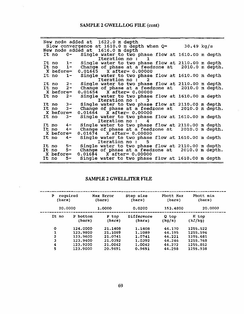
SAMPLE 2 GWELL.LOG FILE (cont)
depthdepth.
depth
30.49 kgjsNew node added at 1622.0 m depth
Slow convergence at 1610.0 m depth when Q=New node added at 1616.0 m depthIt no 0- single water to two phase flow at 1610.00 m depth
Iteration no: 1Single water to two phase flow at 2110.00 m depthChange of phase at a feedzone at 2010.0 m depth.
0.01645 X after= 0.00000Single water to two phase flow at 1610.00 m depth
Iteration no: 2Single water to two phase flow at 2110.00 m depthChange of phase at a feedzone at 2010.0 m depth.
0.01654 X after= 0.00000single water to two phase flow at 1610.00 m depth
Iteration no: 3Single water to two phase flow at 2110.00 m depthChange of phase at a feedzone at 2010.0 m depth.
0.01664 X after= 0.00000Single water to two phase flow at 1610.00 m depth
Iteration no: 4Single water to two phase flow at 2110.00 mChange of phase at a feedzone at 2010.0 m
0.01674 X after= 0.00000Single water to two phase flow at 1610.00 m
Iteration no: 5single water to two phase flow at 2110.00 m depthChange of phase at a feedzone at 2010.0 m depth.
0.01684 X after= 0.00000single water to two phase flow at 1610.00 m depth
It no 2It no 2
X before=It no 2-
It no lIt no 1
X before=It no 1-
It no 3It no 3
X before=It no 3-
It no 4It no 4
X before=It no 4-
It no 5It no 5
X before=It no 5-
SAMPLE 2 GWELL.ITER FILE
P required(bars)
Max Error(bars)
step size(bars)
Pbott Max(bars)
Pbott min(bars)
20.0000 1.0000 0.0200 153.4800 20.0000------------------------------------------------------------------------------
It no P bottom P top Difference Q top H top(bars) (bars) (bars) (kg/s) (kJ/kg)
0 124.0000 21.1408 1.1408 44.170 1255.5221 123.9800 21.1089 1.1089 44.195 1255.5962 123.9600 21.0741 1.0741 44.221 1255.6813 123.9400 21.0392 1.0392 44.246 1255.7684 123.9200 21.0042 1.0042 44.272 1255.8525 123.9000 20.9691 0.9691 44.298 1255.938
69
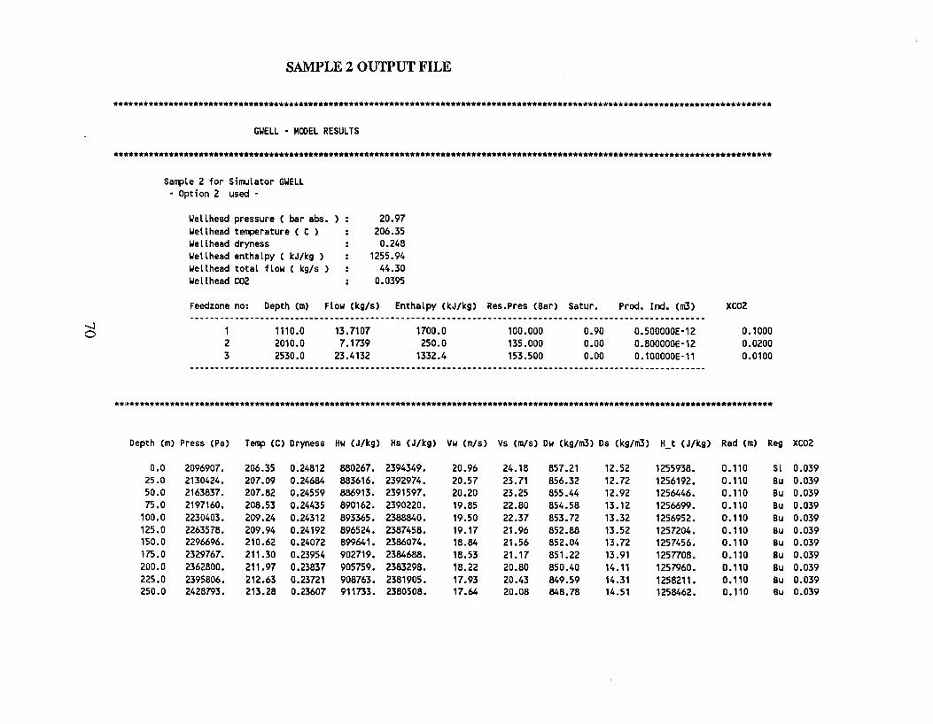
SAMPLE 2 OUTPUT FILE
**-,*************.***********************************************************************************,~*****************************
GWELL - MODEL RESULTS
**j,*******************************************************************************************************************************
Sample 2 for Simulator GWELL• Option 2 used-
Wellhead pressure ( bar abs.Wellhead temperature ( C )Wellhead drynessWellhead enthalpy ( kJ/kg )Wellhead total flow ( kg/s )Wellhead C02
20.97206.350.248
1255.9444.30
0.0395
Feedzone no: Depth (m) Flow (kg/s) Enthalpy (kJ/kg) Res.Pres (Bar) Satur. Prod. Ind. (m3) XC02
-.....Jo 123
1110.02010.02530.0
13.71077.1739
23.4132
1700.0250.0
1332.4
100.000135.000153.500
0.900.000.00
0.500000E-120.800000E-12o.100000E-11
0.10000.02000.0100
**********************************************************************************************************************************
Depth (m) Press (Pa) Temp (C) Dryness Hw (J/kg) Hs (J/kg) Vw (m/s) Vs (m/s) Dw (kg/m3) Ds (kg/m3) H_t (J/kg) Rad (m) Reg XC02
0.0 2096907. 206.35 0.24812 880267. 2394349. 20.96 24.18 857.21 12.52 1255938. 0.110 Sl 0.03925.0 2130424. 207.09 0.24684 883616. 2392974. 20.57 23.71 856.32 12.72 1256192. 0.110 Bu 0.03950.0 2163837. 207.82 0.24559 886913. 2391597. 20.20 23.25 855.44 12.92 1256446. 0.110 Bu 0.03975.0 2197160. 208.53 0.24435 890162. 2390220. 19.85 22.80 854.58 13.12 1256699. 0.110 au 0.039
100.0 2230403. 209.24 0.24312 893365. 2388840. 19.50 22.37 853.72 13.32 1256952. 0.110 au 0.039125.0 2263578. 209.94 0.24192 896524. 2387458. 19.17 21.96 852.88 13.52 1257204. 0.110 au 0.039150.0 2296696. 210.62 0.24072 899641. 2386074. 18.84 21.56 852.04 13.72 1257456. 0.110 au 0.039175.0 2329767. 211.30 0.23954 902719. 2384688. 18.53 21.17 851.22 13.91 1257708. 0.110 au 0.039200.0 2362800. 211.97 0.23837 905759. 2383298. 18.22 20.80 850.40 14.11 1257960. 0.110 au 0.039225.0 2395806. 212.63 0.23721 908763. 2381905. 17.93 20.43 849.59 14.31 1258211. 0.110 au 0.039250.0 2428793. 213.28 0.23607 911733. 2380508. 17.64 20.08 848.78 14.51 1258462. 0.110 au 0.039
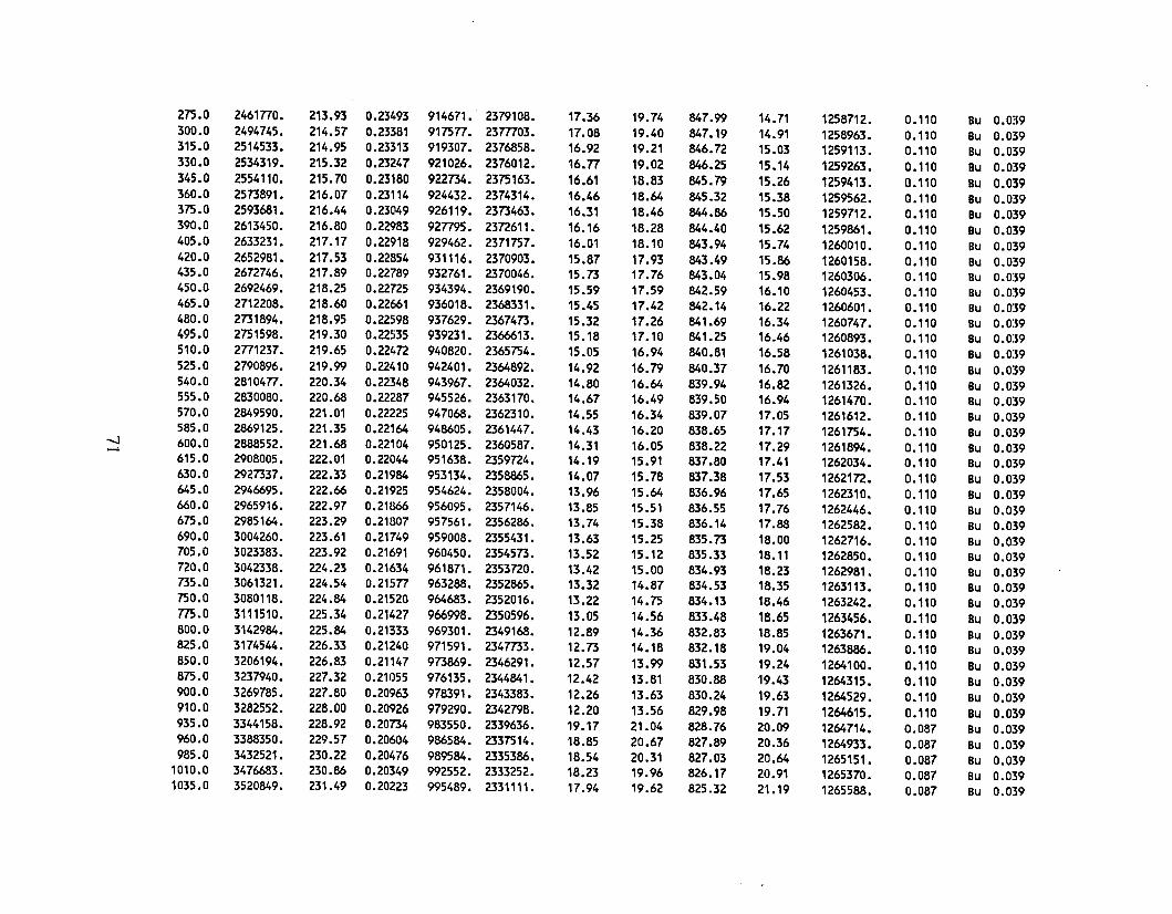
275.0 2461nO. 213.93 0.23493 914671. 2379108. 17.36 19.74 847.99 14.71 1258712. 0.110 Bu 0.039300.0 2494745. 214.57 0.23381 9175n. 23n703. 17.08 19.40 847.19 14.91 1258963. 0.110 Bu 0.039315.0 2514533. 214.95 0.23313 919307. 2376858. 16.92 19.21 846.72 15.03 1259113. 0.110 Bu 0.039330.0 2534319. 215.32 0.23247 921026. 2376012. 16.n 19.02 846.25 15.14 1259263. 0.110 Bu 0.039345.0 2554110. 215.70 0.23180 922734. 2375163. 16.61 18.83 845.79 15.26 1259413. 0.110 Bu 0.039360.0 2573891. 216.07 0.23114 924432. 2374314. 16.46 18.64 845.32 15.38 1259562. 0.110 Bu 0.039375.0 2593681. 216.44 0.23049 926119. 2373463. 16.31 18.46 844.86 15.50 1259712. 0.110 Bu 0.039390.0 2613450. 216.80 0.22983 92m5. 2372611. 16.16 18.28 844.40 15.62 1259861. 0.110 Bu 0.039405.0 2633231. 217.17 0.22918 929462. 2371757. 16.01 18.10 843.94 15.74 1260010. 0.110 Bu 0.0:59420.0 2652981. 217.53 0.22854 931116. 2370903. 15.87 17.93 843.49 15.86 1260158. 0.110 Bu 0.039435.0 2672746. 217.89 0.22789 932761. 2370046. 15.73 17.76 843.04 15.98 1260306. 0.110 Bu 0.039450.0 2692469. 218.25 0.22725 934394. 2369190. 15.59 17.59 842.59 16.10 1260453. 0.110 Bu 0.039465.0 2712208. 218.60 0.22661 936018. 2368331. 15.45 17.42 842.14 16.22 1260601. 0.110 Bu 0.039480.0 2731894. 218.95 0.22598 937629. 2367473. 15.32 17.26 841.69 16.34 1260747. 0.110 Bu 0.039495.0 2751598. 219.30 0.22535 939231. 2366613. 15.18 17.10 841.25 16.46 1260893. 0.110 Bu 0.0:59510.0 2n1237. 219.65 0.22472 940820. 2365754. 15.05 16.94 840.81 16.58 1261038. 0.110 Bu 0.0:59525.0 2790896. 219.99 0.22410 942401. 2364892. 14.92 16.79 840.37 16.70 1261183. 0.110 Bu 0.0:59540.0 2810477. 220.34 0.22348 943967. 2364032. 14.80 16.64 839.94 16.82 1261326. 0.110 Bu 0.0:59555.0 2830080. 220.68 0.22287 945526. 2363170. 14.67 16.49 839.50 16.94 1261470. 0.110 Bu 0.0:59570.0 2849590. 221.01 0.22225 947068. 2362310. 14.55 16.34 839.07 17.05 1261612. 0.110 Bu 0.0:59585.0 2869125. 221.35 0.22164 948605. 2361447. 14.43 16.20 838.65 17.17 1261754. 0.110 Bu 0.0:59
-.....l 600.0 2888552. 221.68 0.22104 950125. 2360587. 14.31 16.05 838.22 17.29 1261894. 0.110 Bu 0.039,....615.0 2908005. 222.01 0.22044 951638. 2359724. 14.19 15.91 837.80 17.41 1262034. 0.110 Bu 0.039630.0 2927337. 222.33 0.21984 953134. 2358865. 14.07 15.78 837.38 17.53 1262172. 0.110 Bu 0.039645.0 2946695. 222.66 0.21925 954624. 2358004. 13.96 15.64 836.96 17.65 1262310. 0.110 Bu 0.039660.0 2965916. 222.97 0.21866 956095. 2357146. 13.85 15.51 836.55 17.76 1262446. 0.110 Bu 0.039675.0 2985164. 223.29 0.21807 957561. 2356286. 13.74 15.38 836.14 17.88 1262582. 0.110 Bu 0.039690.0 3004260. 223.61 0.21749 959008. 2355431. 13.63 15.25 835.73 18.00 1262716. 0.1'0 Bu 0.039705.0 3023383. 223.92 0.21691 960450. 2354573. 13.52 15.12 835.33 18.11 1262850. 0.110 Bu 0.039720.0 3042338. 224.23 0.21634 961871. 2353720. 13.42 15.00 834.93 18.23 1262981. 0.110 Bu 0.039735.0 3061321. 224.54 0.21577 963288. 2352865. 13.32 14.87 834.53 18.35 1263113. 0.110 Bu 0.039750.0 3080118. 224.84 0.21520 964683. 2352016. 13.22 14.75 834.13 18.46 1263242. 0.110 Bu 0.039m.o 3111510. 225.34 0.21427 966998. 2350596. 13.05 14.56 833.48 18.65 1263456. 0.110 Bu 0.039800.0 3142984. 225.84 0.21333 969301. 2349168. 12.89 14.36 832.83 18.85 1263671. 0.110 Bu 0.039825.0 3174544. 226.33 0.21240 971591. 234m3. 12.73 14.18 832.18 19.04 1263886. 0.110 Bu 0.039850.0 3206194. 226.83 0.21147 973869. 2346291. 12.57 13.99 831.53 19.24 1264100. 0.110 Bu 0.039875.0 3237940. 227.32 0.21055 976135. 2344841. 12.42 13.81 830.88 19.43 1264315. 0.110 Bu 0.039900.0 3269785. 227.80 0.20963 978391. 2343383. 12.26 13.63 830.24 19.63 1264529. 0.110 Bu 0.039910.0 3282552. 228.00 0.20926 979290. 2342798. 12.20 13.56 829.98 19.71 1264615. 0.110 Bu 0.039935.0 3344158. 228.92 0.20734 983550. 2339636. 19.17 21.04 828.76 20.09 1264714. 0.087 Bu 0.039960.0 3388350. 229.57 0.20604 986584. 2337514. 18.85 20.67 827.89 20.36 1264933. 0.087 Bu 0.039985.0 3432521. 230.22 0.20476 989584. 2335386. 18.54 20.31 827.03 20.64 1265151. 0.087 Bu 0.039
1010.0 3476683. 230.86 0.20349 992552. 2333252. 18.23 19.96 826.17 20.91 1265370. 0.087 Bu 0.0391035.0 3520849. 231.49 0.20223 995489. 2331111. 17.94 19.62 825.32 21.19 1265588. 0.087 Bu 0.039
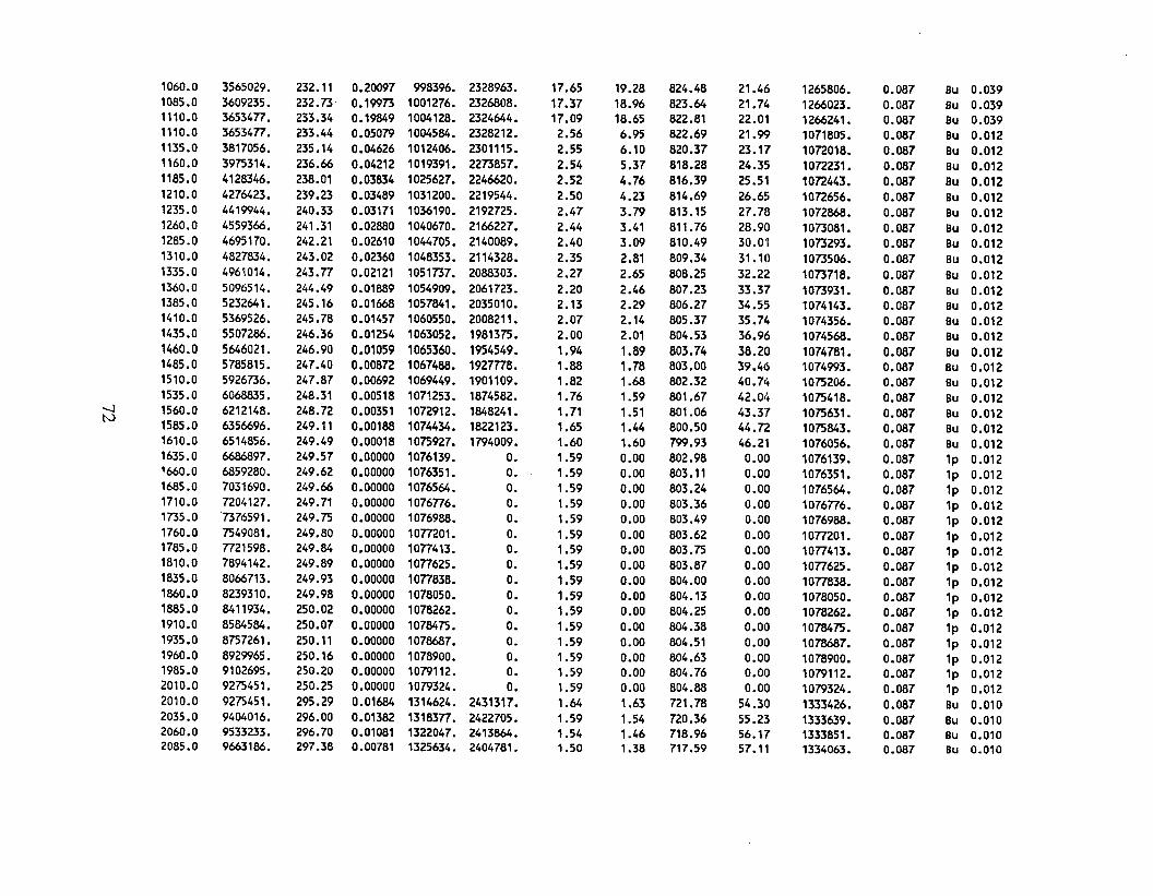
1060.0 3565029. 232.11 0.20097 998396. 2328963. 17.65 19.28 824.48 21.46 1265806. 0.087 Bu 0.0391085.0 3609235. 232.73 0.19973 1001276. 2326808. 17.37 18.96 823.64 21.74 1266023. 0.087 Bu 0.0391110.0 36534IT. 233.34 0.19849 1004128. 2324644. 17.09 18.65 822.81 22.01 1266241. 0.087 Bu 0.0391110.0 36534IT. 233.44 0.05079 1004584. 2328212. 2.56 6.95 822.69 21.99 1071805. 0.087 Bu 0.0121135.0 3817056. 235.14 0.04626 1012406. 2301115. 2.55 6.10 820.37 23.17 1072018. 0.087 au 0.0121160.0 3975314. 236.66 0.04212 1019391. 2273857. 2.54 5.37 818.28 24.35 1072231. 0.087 Bu 0.0121185.0 4128346. 238.01 0.03834 1025627. 2246620. 2.52 4.76 816.39 25.51 1072443. 0.087 au 0.0121210.0 4276423. 239.23 0.03489 1031200. 2219544. 2.50 4.23 814.69 26.65 1072656. 0.087 Bu 0.0121235.0 4419944. 240.33 0.03171 1036190. 2192725. 2.47 3.79 813.15 27.78 1072868. 0.087 Bu 0.0121260.0 4559366. 241.31 0.02880 1040670. 2166227. 2.44 3.41 811.76 28.90 1073081. 0.087 Bu 0.0121285.0 4695170. 242.21 0.02610 1044705. 2140089. 2.40 3.09 810.49 30.01 1073293. 0.087 Bu 0.0121310.0 4827834. 243.02 0.02360 1048353. 2114328. 2.35 2.81 809.34 31.10 1073506. 0.087 Bu 0.0121335.0 4961014. 243.IT 0.02121 1051737. 2088303. 2.27 2.65 808.25 32.22 1073718. 0.087 Bu 0.0121360.0 5096514. 244.49 0.01889 1054909. 2061723. 2.20 2.46 807.23 33.37 1073931. 0.087 Bu 0.0121385.0 5232641. 245.16 0.01668 1057841. 2035010. 2.13 2.29 806.27 34.55 1074143. 0.087 Bu 0.0121410.0 5369526. 245.78 0.01457 1060550. 2008211. 2.07 2.14 805.37 35.74 1074356. 0.087 Bu 0.0121435.0 5507286. 246.36 0.01254 1063052. 1981375. 2.00 2.01 804.53 36.96 1074568. 0.087 Bu 0.0121460.0 5646021. 246.90 0.01059 1065360. 1954549. 1.94 1.89 803.74 38.20 1074781. 0.087 au 0.0121485.0 5785815. 247.40 0.00872 1067488. 192m8. 1.88 1.78 803.00 39.46 1074993. 0.087 Bu 0.0121510.0 5926736. 247.87 0.00692 1069449. 1901109. 1.82 1.68 802.32 40.74 1075206. 0.087 Bu 0.0121535.0 6068835. 248.31 0.00518 1071253. 1874582. 1.76 1.59 801.67 42.0/. 1075418. 0.087 au 0.012
-.l 1560.0 6212148. 248.72 0.00351 1072912. 1848241. 1.71 1.51 801.06 43.37 1075631. 0.087 Bu 0.012tv 1585.0 6356696. 249.11 0.00188 1074434. 1822123. 1.65 1.44 800.50 44.72 1075843. 0.087 Bu 0.0121610.0 6514856. 249.49 0.00018 1075927. 1794009. 1.60 1.60 799.93 46.21 1076056. 0.087 Bu 0.0121635.0 6686897. 249.57 0.00000 1076139. o. 1.59 0.00 802.98 0.00 1076139. 0.087 1p 0.0121660.0 6859280. 249.62 0.00000 1076351. o. 1.59 0.00 803.11 0.00 1076351. 0.087 lp 0.0121685.0 7031690. 249.66 0.00000 1076564. o. 1.59 0.00 803.24 O.OiJ 1076564. 0.087 1p 0.0121710.0 7204127. 249.71 0.00000 1076IT6. o. 1.59 0.00 803.36 0.00 1076IT6. 0.087 1p 0.0121735.0 '7376591. 249.75 0.00000 1076988. o. 1.59 0.00 803.49 0.00 1076988. 0.087 lp 0.0121760.0 7549081. 249.80 0.00000 10mOl. o. 1.59 0.00 803.62 0.00 10IT201. 0.087 lp 0.0121785.0 m1598. 249.84 0.00000 10IT413. o. 1.59 0.00 803.75 0.00 10IT413. 0.087 1p 0.0121810.0 7894142. 249.89 0.00000 10IT625. o. 1.59 0.00 803.87 0.00 10IT625. 0.087 lp 0.0121835.0 8066713. 249.93 0.00000 10IT838. o. 1.59 0.00 804.00 0.00 10IT838. 0.087 lp 0.0121860.0 8239310. 249.98 0.00000 1078050. o. 1.59 0.00 804.13 0.00 1078050. 0.087 lp 0.0121885.0 8411934. 250.02 0.00000 1078262. o. 1.59 0.00 804.25 0.00 1078262. 0.087 lp 0.0121910.0 8584584. 250.07 0.00000 1078475. o. 1.59 0.00 804.38 0.00 1078475. 0.087 lp 0.0121935.0 8757261. 250.11 0.00000 1078687. o. 1.59 0.00 804.51 0.00 1078687. 0.087 1p 0.0121960.0 8929965. 250.16 0.00000 1078900. O. 1.59 0.00 804.63 0.00 1078900. 0.087 1p 0.0121985.0 9102695. 250.20 0.00000 1079112. o. 1.59 0.00 804.76 0.00 1079112. 0.087 lp 0.0122010.0 9275451. 250.25 0.00000 1079324. o. 1.59 0.00 804.88 0.00 1079324. 0.087 1p 0.0122010.0 9275451. 295.29 0.01684 1314624. 2431317. 1.64 1.63 721.78 54.30 1333426. 0.087 au 0.0102035.0 9404016. 296.00 0.01382 13183IT. 2422705. 1.59 1.54 720.36 55.23 1333639. 0.087 au 0.0102060.0 9533233. 296.70 0.01081 1322047. 2413864. 1.54 1.46 718.96 56.17 1333851- 0.087 Bu 0.0102085.0 9663186. 297.38 0.00781 1325634. 2404781. 1.50 1.38 717.59 57.11 1334063. 0.087 Bu 0.010

2110.0 9801154. 298.07 0.00465 1329322. 2394901. 1.37 1.37 716.17 58.13 1334276. 0.087 au 0.0102135.0 9954724. 298.51 0.00000 1329532. 2402845. 1.36 1.36 718.65 57.20 1329532. 0.087 1p 0.0102160.0 10108580. 298.58 0.00000 1329745. 2392872. 1.36 1.36 718.83 58.22 1329745. 0.087 1p 0.0102185.0 10262472. 298.65 0.00000 1329957. O. 1.36 0.00 719.01 0.00 1329957. 0.087 1p 0.0102210.0 10416403. 298.71 0.00000 1330169. O. 1.36 0.00 719.19 0.00 1330169. 0.087 1p 0.0102235.0 10570371. 298.78 0.00000 1330381. O. 1.36 0.00 719.36 0.00 1330381. 0.087 1p 0.0102260.0 10724376. 298.85 0.00000 1330593. O. 1.36 0.00 719.54 0.00 1330593. 0.087 1p 0.0102285.0 10878419. 298.91 0.00000 1330805. O. 1.36 0.00 719.72 0.00 1330805. 0.087 1p 0.0102310.0 11032499. 298.98 0.00000 1331017. O. 1.36 0.00 719.90 0.00 1331017• 0.087 1p 0.0102335.0 11186616. 299.05 0.00000 1331230. O. 1.36 0.00 720.07 0.00 1331230. 0.087 1p 0.0102360.0 11340nO. 299.11 0.00000 1331442. O. 1.36 0.00 720.25 0.00 1331442. 0.087 1p 0.0102385.0 11494962. 299.18 0.00000 1331654. O. 1.36 0.00 720.42 0.00 1331654. 0.087 1p 0.0102410.0 11649190. 299.25 0.00000 1331866. O. 1.36 0.00 720.60 0.00 1331866. 0.087 1p 0.0102435.0 11803456. 299.31 0.00000 1332078. O. 1.36 0.00 720.n 0.00 1332078. 0.087 1p 0.0102460.0 11957758. 299.38 0.00000 1332290. O. 1.36 0.00 720.95 0.00 1332290. 0.087 1p 0.0102485.0 12112097. 299.45 0.00000 1332503. O. 1.36 0.00 721.12 0.00 1332503. 0.087 1p 0.0102510.0 12266473. 299.51 0.00000 1332715. O. 1.36 0.00 721.30 0.00 1332715. 0.087 1p 0.0102530.0 12390000. 299.57 0.00000 1332884. O. 1.36 24.11 721.44 0.00 1332884. 0.087 1p 0.0102530.0 12390000. 299.57 0.00000 1332884. O. 1.36 24.11 721.44 0.00 1332884. 0.087 1p 0.010
-...)t,;J
APPENDIXB
(SAMPLE RUNS FOR GWNACL)
74
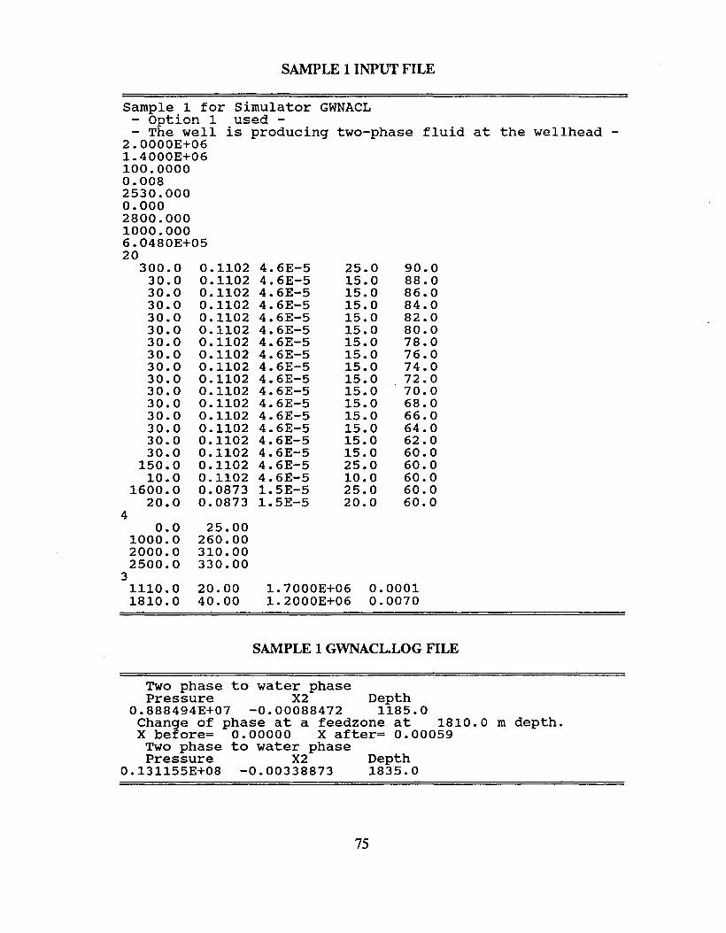
SAMPLE 1 INPUT FILE
fluid at the wellhead -
90.088.086.084.082.080.078.076.074.072.070.068.066.064.062.060.060.060.060.060.0
25.015.015.015.015.015.015.015.015.015.015.015.015.015.015.015.025.010.025.020.0
4.6E-54.6E-54.6E-54.6E-54.6E-54.6E-54.6E-54.6E-54.6E-54.6E-54.6E-54.6E-54.6E-54.6E-54.6E-54.6E-54.6E-54.6E-51. 5E-51. 5E-5
0.11020.11020.11020.11020.11020.11020.11020.11020.11020.11020.11020.11020.11020.11020.11020.11020.11020.11020.08730.0873
Sample 1 for simulator GWNACL- option 1 used-- The well is producing two-phase
2.0000E+061.4000E+06100.00000.0082530.0000.0002800.0001000.0006.0480E+0520
300.030.030.030.030.030.030.030.030.030.030.030.030.030.030.030.0
150.010.0
1600.020.0
40.0
1000.02000.02500.0
31110.01810.0
25.00260.00310.00330.00
20.0040.00
1.7000E+061.2000E+06
0.00010.0070
SAMPLE 1 GWNACL.LOG FILE
Two phase to water phasePressure X2 Depth
0.888494E+07 -0.00088472 1185.0Change of phase at a feedzone at 1810.0 m depth.X before= 0.00000 X after= 0.00059
Two phase to water phasePressure X2 Depth
0.131155E+08 -0.00338873 1835.0
75
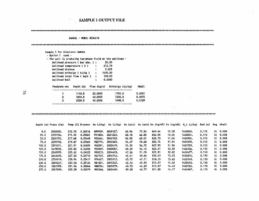
SAMPLE 1 OUTPUT FILE
**********************************************************************************************************************************
GWNACL - MODEL RESULTS
**********************************************************************************************************************************
Sample 1 for Simulator GWNACLOption 1 used·The well is producing two-phase fluid at the wellhead·
Wellhead pressure ( bar abs. ) : 20.00Wellhead temperature ( C ) : 212.70Weqhead dryness : 0.263Wellhead enthalpy ( kJ/kg) : 1400.00Wellhead total flow ( kg/s): 100.00Wellhead NaCl : 0.0080
Feedzone no: Depth (m) Flow (kg/s) Enthalpy (kJ/kg) XNaCl
-.....l0\ 1
23
1110.01810.02530.0
20.000040.000040.0000
1700.01200.01498.9
0.00010.00700.0129
**~r************.************************************* **************************************************************************.***
Oepth (m) Press (Pa) Temp (C) Dryness Hw (J/kg) Hs (J/kg) Vw (mls) Vs (mls) Dw (kg/m3) Os (l<g/m3) H_t (J/kg) Rad em) Reg XNaCl
0.0 2000000. 212.70 0.26316 899939. 2800127. 63.96 71.30 840.44 10.03 1400000. 0.110 Sl 0.00825.0 2105104. 215.30 0.25865 911800. 2801222. 60.18 66.83 836.95 10.55 1400501. 0.110 Sl 0.00850.0 2204725. 217.68 0.25448 922664. 2802122. 56.92 63.01 833.73 11.04 1400954. 0.110 Sl 0.00875.0 2299792. 219.87 0.25060 932715. 2802865. 54.07 59.68 830.74 11.51 1401370. 0.110 Sl 0.008
100.0 2391011. 221.91 0.24695 942091. 2803479. 51.55 56.75 827.95 11.96 1401759. 0.110 Sl 0.008125.0 2478932. 223.82 0.24350 950897. 2803987. 49.29 54.13 825.31 12.39 1402126. 0.110 Sl 0.008150.0 2563995. 225.62 0.24023 959213. 2804403. 47.26 51.78 822.81 12.82 1402477. 0.110 Sl 0.008175.0 2646559. 227.32 0.23710 967105. 2804742. 45.41 49.66 820.43 13.23 1402814. 0.110 Sl 0.008200.0 2726919. 228.94 0.23411 974627. 2805012. 43.72 47.71 818.15 13.63 1403140. 0.110 Sl 0.008225.0 2805327. 230.48 0.23124 981821. 2805222. 42.16 45.93 815.97 14.02 1403456. 0.110 Sl 0.008250.0 2881993. 231.96 0.22846 988724. 2805379. 40.72 44.29 813.87 14.40 1403765. 0.110 Sl 0.008275.0 2957099. 233.38 0.22579 995366. 2805489. 39.38 42.77 811.85 14.77 1404067. 0.110 Sl 0.008
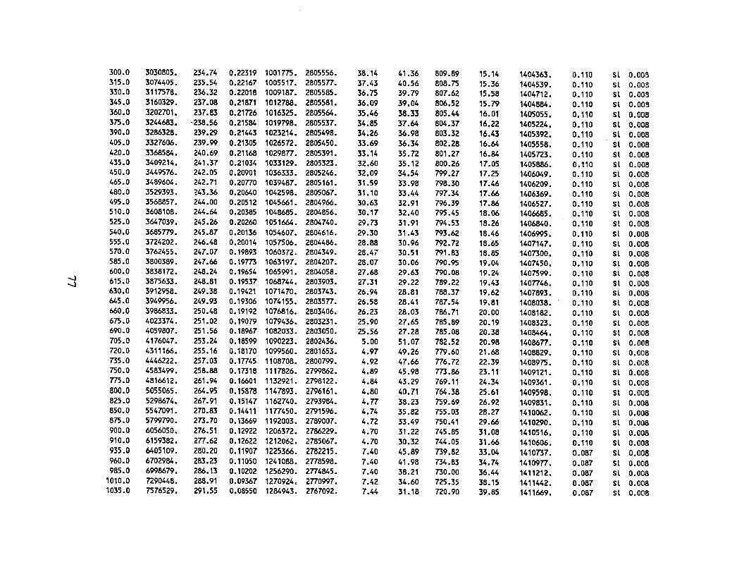
300.0 3030805. 234.74 0.22319 1001775. 2805556. 38.14 41.36 809.89 15.14 1404363. 0.110 Sl 0.008315.0 3074405. 235.54 0.22167 1005517. 2805577. 37.43 40.56 808.75 15.36 1404539. 0.110 Sl 0.008330.0 3117578. 236.32 0.22018 1009187. 2805585. 36.75 39.79 807.62 15.58 1404712. 0.110 Sl 0.008345.0 3160329. 237.08 0.21871 1012788. 2805581. 36.09 39.04 806.52 15.79 1404884. 0.110 Sl 0.008360.0 3202701. 237.83 0.21726 1016325. 2805564. 35.46 38.33 805.44 16.01 1405055. 0.110 Sl 0.008375.0 3244683. -238.56 0.21584 1019798. 2805537. 34.85 37.64 804.37 16.22 1405224. 0.110 Sl 0.008390.0 3286328. 239.29 0.21443 1023214. 2805498. 34.26 36.98 803.32 16.43 1405392. 0.110 Sl 0.008405.0 3327606. 239.99 0.21305 1026572. 2805450. 33.69 36.34 802.28 16.64 1405558. 0.110 Sl 0.00.8420.0 3368584. 240.69 0.21168 1029877. 2805391. 33.14 35.72 801.27 16.84 1405n3. 0.110 Sl 0.008435.0 3409214. 241.37 0.21034 1033129. 2805323. 32.60 35.12 800.26 17.05 1405886. 0.110 Sl 0.008450.0 3449576. 242.05 0.20901 1036333. 2805246. 32.09 34.54 799.27 17.25 1406049. 0.110 Sl 0.008465.0 3489604. 242.71 0.20770 1039487. 2805161. 31.59 33.98 798.30 17.46 1406209. 0.110 Sl 0.008480.0 3529393. ~43.36 0.20640 1042598. 2805067. 31.10 33.44 797.34 17.66 1406369. 0.110 Sl 0.008495.0 3568857. 244.00 0.20512 1045661. 2804966. 30.63 32.91 796.39 17.86 1406527. 0.110 Sl 0.008510.0 3608108. 244.64 0.20385 1048685. 2804856. 30.17 32.40 795.45 18.06 1406685. 0.110 Sl 0.008525.0 3647039. 245.26 0.20260 1051664. 2804740. 29.73 31.91 794.53 18.26 14Q.6840. 0.110 Sl 0.008540.0 3685779. 245.87 0.20136 1054607. 2804616. 29.30 31.43 793.62 18.46 1406995. 0.110 Sl 0.008555.0 3724202. 246.48 0.20014 1057506. 2804486. 28.88 30.96 792.72 18.65 1407147. 0.110 Sl 0.008570.0 3762455. 247.07 0.19893 1060372. 2804349. 28.47 30.51 791.83 18.85 1407300. 0.110 Sl 0.008585.0 3800389. 247.66 0.19m 1063197. 2804207. 28.07 30.06 790.95 19.04 1407450. 0.110 Sl 0.008600.0 3838172. 248.24 0.19654 1065991. 2804058. 27.68 29.63 790.08 19.24 1407599. 0.110 Sl 0.008
-..) 615.0 3875633. 248.81 0.19537 1068744. 2803903. 27.31 29.22 789.22 19.43 1407746. 0.110 Sl 0.008-..)630.0 3912958. 249.38 0.19421 1071470. 2803743. 26.94 28.81 788.37 19.62 1407893. 0.110 Sl 0.008645.0 3949956. 249.93 0.19306 1074155. 2803577. 26.58 28.41 787.54 19.81 1408038. 0.110 Sl 0.008660.0 3986833. 250.48 0.19192 1076816. 2803406. 26.23 28.03 786.71 20.00 1408182. 0.110 Sl 0.008675.0 4023374. 251.02 0.19079 1079436. 2803231- 25.90 27.65 785.89 20.19 1408323. 0.110 Sl 0.008690.0 4059807. 251.56 0.18967 1082033. 2803050. 25.56 27.28 785.08 20.38 1408464. 0.110 Sl 0.008705.0 4176047. 253.24 0.18599 1090223. 2802436. 5.00 51.07 782.52 20.98 1408677. 0.110 Sl 0.008720.0 4311166. 255.16 0.18170 1099560. 2801653. 4.97 49.26 779.60 21.68 1408829. 0.110 Sl 0.008735.0 4446222. 257.03 0.17745 1108708. 2800799. 4.92 47.66 776.72 22.39 1408975. 0.110 Sl 0.008750.0 4583499. 258.88 0.17318 1117826. 2799862. 4.89 45.98 773.86 23.11 1409121. 0.110 Sl 0.008775.0 4816612. 261.94 0.16601 1132921. 2798122. 4.84 43.29 769.11 24.34 1409361. 0.110 Sl 0.008800.0 5055065. 264.95 0.15878 1147893. 2796161. 4.80 40.71 764.38 25.61 1409598. 0.110 Sl 0.008825.0 5298674. 267.91 0.15147 1162740. 2793984. 4.77 38.23 759.69 26.92 1409831. 0.110 Sl 0.008850.0 5547091. 270.83 0.14411 1177450. 2791596. 4.74 35.82 755.03 28.27 1410062. 0.110 Sl 0.008875.0 5799790. 273.70 0.13669 1192003. 2789007. 4.72 33.49 750.41 29.66 1410290. 0.110 Sl 0.008900.0 6056050. 276.51 0.12922 1206372. 2786229. 4.70 31.22 745.85 31.08 1410516. 0.110 Sl 0.008910.0 6159382. 277.62 0.12622 1212062. 2785067. 4.70 30.32 744.05 31.66 1410606. 0.110 Sl 0.008935.0 6405109. 280.20 0.11907 1225366. 2782215. 7.40 45.89 739.82 33.04 1410737. 0.007 Sl 0.008960.0 6702984. 283.23 0.11050 1241088. 2778598. 7.40 41.98 734.83 34.74 1410977. 0.087 Sl 0.008985.0 6998679. 286.13 0.10202 1256290. 2774845. 7.40 38.21 730.00 36.44 1411212. 0.087 Sl 0.008
1010.0 n90448. 288.91 0.09367 1270924. 2770997. 7.42 34.60 725.35 38.15 1411442. 0.087 Sl 0.0081035.0 7576529. 291.55 0.08550 1284943. 2767092. 7.44 31.18 720.90 39.85 1411669. 0.087 Sl 0.008
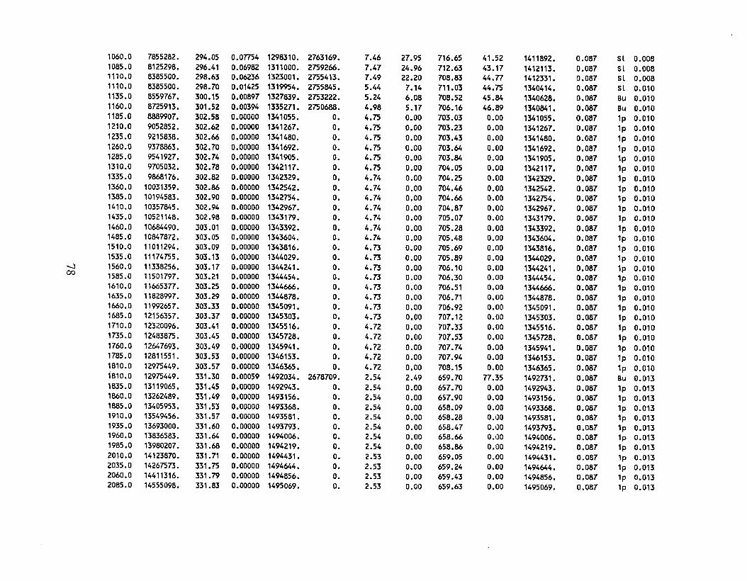
1060.0 7855282. 294.05 0.Om4 1298310. 2763169. 7.46 27.95 716.65 41.52 1411892. 0.087 5l 0.0081085.0 8125298. 296.41 0.06982 1311000. 2759266. 7.47 24.96 712.63 43.17 1412113. 0.087 5l 0.0081110.0 8385500. 298.63 0.06236 1323001. 2755413. 7.49 22.20 708.83 44.77 1412331. 0.087 5l 0.0081110.0 8385500. 298.70 0.01425 1319954. 2755845. 5.44 7.14 711.03 44.7'5 1340414. 0.087 5l 0.0101135.0 8559767. 300.15 0.00897 1327839. 2753222. 5.24 6.08 708.52 45.84 1340628. 0.087 Bu 0.0101160.0 8725913. 301.52 0.00394 1335271. 2750688. 4.98 5.17 706.16 46.89 1340841. 0.087 Bu 0.0101185.0 8889907. 302.58 0.00000 1341055. O. 4.75 0.00 703.03 0.00 1341055. 0.087 1p 0.0101210.0 9052852. 302.62 0.00000 1341267. O. 4.75 0.00 703.23 0.00 1341267. 0.087 1p 0.0101235.0 9215838. 302.66 0.00000 1341480. O. 4.75 0.00 703.43 0.00 1341480. 0.087 1p 0.0101260.0 9378863. 302.70 0.00000 1341692. O. 4.75 0.00 703.64 0.00 1341692. 0.087 1p 0.0101285.0 9541927. 302.74 0.00000 1341905. O. 4.75 0.00 703.84 0.00 1341905. 0.087 1p 0.0101310.0 9705032. 302.78 0.00000 1342117. O. 4.75 0.00 704.05 0.00 1342117. 0.087 1p 0.0101335.0 9868176. 302.82 0.00000 1342329. O. 4.74 0.00 704.25 0.00 1342329. 0.087 1p 0.0101360.0 10031359. 302.86 0.00000 1342542. O. 4.74 0.00 704.46 0.00 1342542. 0.087 1p 0.0101385.0 10194583. 302.90 0.00000 1342754. O. 4.74 0.00 704.66 0.00 1342754. 0.087 1p 0.0101410.0 10357845. 302.94 0.00000 1342967. O. 4.74 0.00 704.87 0.00 1342967. 0.087 1p 0.0101435.0 10521148. 302.98 0.00000 1343179. O. 4.74 0.00 705.07 0.00 1343179. 0.087 lp 0.0101460.0 10684490. 303.01 0.00000 1343392. O. 4.74 0.00 705.28 0.00 1343392. 0.087 1p 0.0101485.0 10847872. 303.05 0.00000 1343604. O. 4.74 0.00 705.48 0.00 1343604. 0.087 1p 0.0101510.0 11011294. 303.09 0.00000 1343816. O. 4.73 0.00 705.69 0.00 1343816. 0.087 1p 0.0101535.0 11174755. 303.13 0.00000 1344029. O. 4.73 0.00 705.89 0.00 1344029. 0.087 1p 0.010
-.....) 1560.0 11338256. 303.17 0.00000 1344241. O. 4.73 0.00 706.10 0.00 1344241. 0.087 1p 0.01000 1585.0 11501797. 303.21 0.00000 1344454. O. 4.73 0.00 706.30 0.00 1344454. 0.087 1p 0.010
1610.0 11665377. 303.25 0.00000 1344666. O. 4.73 0.00 706.51 0.00 1344666. 0.087 1p 0.0101635.0 11828997. 303.29 0.00000 1344878. O. 4.73 0.00 706.71 0.00 1344878. 0.087 1p 0.0101660.0 11992657. 303.33 0.00000 1345091. O. 4.73 0.00 706.92 0.00 1345091. 0.087 1p 0.0101685.0 12156357. 303.37 0.00000 1345303. O. 4.73 0.00 707.12 0.00 1345303. 0.087 1p 0.0101710.0 12320096. 303.41 0.00000 1345516. O. 4.72 0.00 707.33 0.00 1345516. 0.087 1p 0.0101735.0 12483875. 303.45 0.00000 1345728. O. 4.72 0.00 707.53 0.00 1345728. 0.087 1p 0.0101760.0 12647693. 303.49 0.00000 1345941. O. 4.72 0.00 707.74 0.00 1345941. 0.087 1p 0.0101785.0 12811551. 303.53 0.00000 1346153. O. 4.72 0.00 707.94 0.00 1346153. 0.087 1p 0.0101810.0 12975449. 303.57 0.00000 1346365. O. 4.72 0.00 708.15 0.00 1346365. 0.087 1p 0.0101810.0 12975449. 331.30 0.00059 1492034. 2678709. 2.54 2.49 659.70 77.35 1492731. 0.087 Bu 0.0131835.0 13119065. 331.45 0.00000 1492943. O. 2.54 0.00 657.70 0.00 1492943. 0.087 1p 0.0131860.0 13262489. 331.49 0.00000 1493156. O. 2.54 0.00 657.90 0.00 1493156. 0.087 1p 0.0131885.0 13405953. 331.53 0.00000 1493368. O. 2.54 0.00 658.09 0.00 1493368. 0.087 1p 0.0131910.0 13549456. 331.57 0.00000 1493581. O. 2.54 0.00 658.28 0.00 1493581. 0.087 1p 0.0131935.0 13693000. 331.60 0.00000 1493793. O. 2.54 0.00 658.47 0.00 1493793. 0.087 1p 0.0131960.0 13836583. 331.64 0.00000 1494006. O. 2.54 0.00 658.66 0.00 1494006. 0.087 1p 0.0131985.0 13980207. 331.68 0.00000 1494219. O. 2.54 0.00 658.86 0.00 1494219. 0.087 1p 0.0132010.0 14123870. 331.71 0.00000 1494431. O. 2.53 0.00 659.05 0.00 1494431. 0.087 1p 0.0132035.0 14267573. 331.75 0.00000 1494644. O. 2.53 0.00 659.24 0.00 1494644. 0.087 1p 0.0132060.0 14411316. 331.79 0.00000 1494856. O. 2.53 0.00 659.43 0.00 1494856. 0.087 1p 0.0132085.0 14555098. 331.83 0.00000 1495069. O. 2.53 0.00 659.63 0.00 1495069. 0.087 1p 0.013
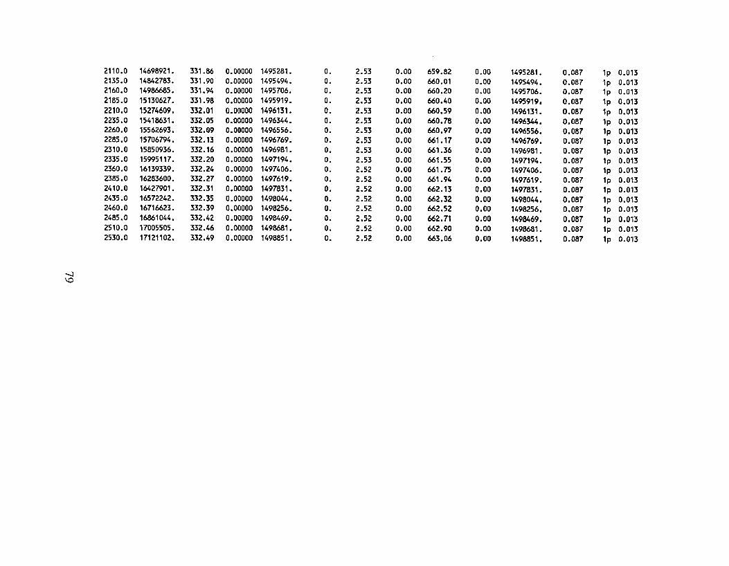
-....)\0
2110.0 14698921. 331.86 0.00000 1495281. o. 2.53 0.00 659.82 0.00 1495281. 0.087 1p 0.0132135.0 14842783. 331.90 0.00000 1495494. o. 2.53 0.00 660.01 0.00 1495494. 0.087 1p 0.0132160.0 14986685. 331.94 0.00000 1495706. o. 2.53 0.00 660.20 0.00 1495706. 0.087 1p 0.0132185.0 15130627. 331.98 0.00000 1495919. o. 2.53 0.00 660.40 0.00 1495919. 0.087 1p 0.0132210.0 15274609. 332.01 0.00000 1496131. o. 2.53 0.00 660.59 0.00 1496131. 0.087 1p 0.0132235.0 15418631. 332.05 0.00000 1496344. o. 2.53 0.00 660.78 0.00 1496344. 0.087 1p 0.0132260.0 15562693. 332.09 0.00000 1496556. o. 2.53 0.00 660.97 0.00 1496556. 0.087 1p 0.0132285.0 15706794. 332.13 0.00000 1496769. o. 2.53 0.00 661.17 0.00 1496769. 0.087 1p 0.0132310.0 15850936. 332.16 0.00000 1496981. o. 2.53 0.00 661.36 0.00 1496981. 0.087 1p 0.0132335.0 15995117. 332.20 0.00000 1497194. o. 2.53 0.00 661.55 0.00 1497194. 0.087 1p 0.0132360.0 16139339. 332.24 0.00000 1497406. o. 2.52 0.00 661.75 0.00 1497406. 0.087 1p 0.0132385.0 16283600. 332.27 0.00000 1497619. O. 2.52 0.00 661.94 0.00 1497619. 0.087 1p 0.0132410.0 16427901. 332.31 0.00000 1497831. O. 2.52 0.00 662.13 0.00 1497831. 0.087 1p 0.0132435.0 16572242. 332.35 0.00000 1498044. o. 2.52 0.00 662 •.32 0.00 1498044. 0.087 1p 0.0132460.0 16716623. 332.39 0.00000 1498256. o. 2.52 0.00 662.52 0.00 1498256. 0.087 1p 0.0132485.0 16861044. 332.42 0.00000 1498469. o. 2.52 0.00 662.71 0.00 1498469. 0.087 1p 0.01132510.0 17005505. 332.46 0.00000 1498681. o. 2.52 0.00 662.90 0.00 1498681. 0.087 1p 0.0132530.0 17121102. 332.49 0.00000 1498851. O. 2.52 0.00 663.06 0.00 1498851. 0.087 1p 0.013
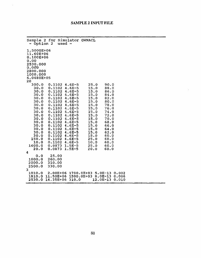
SAMPLE 2 INPUT FILE
Sample 2 for Simulator GWNACL- option 2 used -
1.5000E+0611.60E+060.100E+060.002530.0000.00"02800.0001000.0006.0480E+0520
300.0 0.1102 4.6E-5 25.0 90.030.0 0.1102 4.6E-5 15.0 88.030.0 0.1102 4.6E-5 15.0 86.030.0 0.1102 4.6E-5 15.0 84.030.0 0.1102 4.6E-5 15.0 82.030.0 0.1102 4.6E-5 15.0 80.030.0 0.1102 4.6E-5 15.0 78.030.0 0.1102 4.6E-5 15.0 76.030.0 0.1102 4.6E-5 15.0 74.030.0 0.1102 4.6E-5 15.0 72.030.0 0.1102 4.6E-5 15.0 70.030.0 0.1102 4.6E-5 15.0 68.030.0 0.1102 4.6E-5 15.0 66.030.0 0.1102 4.6E-5 15.0 64.030.0 0.1102 4.6E-5 15.0 62.030.0 0.1102 4.6E-5 15.0 60.0
150.0 0.1102 4.6E-5 25.0 60.010.0 0.1102 4.6E-5 10.0 60.0
1600.0 0.0873 1. 5E-5 25.0 60.020.0 0.0873 1.5E-5 20.0 60.0
40.0 25.00
1000.0 260.002000.0 310.002500.0 330.00
31010.0 2.00E+06 1700.0E+03 5.0E-13 0.0021810.0 11. 50E+06 1500.0E+03 8.0E-13 0.0062530.0 14.35E+06 310.0 12.0E-13 0.010
80
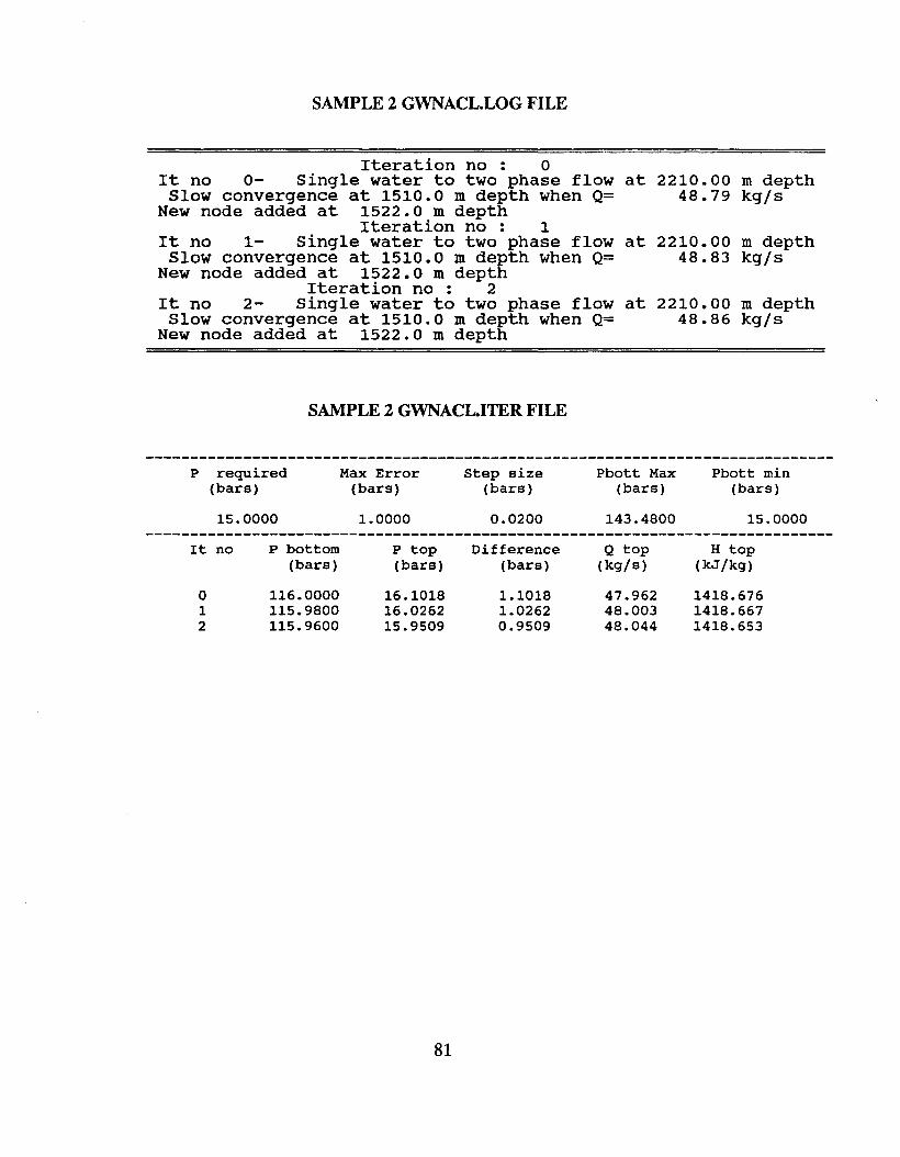
SAMPLE 2 GWNACL.LOG FILE
Iteration no: 0It no 0- Single water to two phase flow
Slow convergence at 1510.0 m depth when Q=New node added at 1522.0 m depth
Iteration no: 1It no 1- Single water to two phase flow
Slow convergence at 1510.0 m depth when Q=New node added at 1522.0 m depth
Iteration no: 2It no 2- Single water to two phase flow
Slow convergence at 1510.0 m depth when Q=New node added at 1522.0 m depth
SAMPLE 2 GWNACL.lTER FILE
at 2210.00 m depth48.79 kg/s
at 2210.00 m depth48.83 kg/s
at 2210.00 m depth48.86 kg/s
P required(bars)
15.0000
Max Error(bars)
1.0000
Step size(bars)
0.0200
Pbott Max(bars)
143.4800
Pbott min(bars)
15.0000------------------------------------------------------------------------------
It no P bottom P top Difference Q top H top(bars) (bars) (bars) (kg/B) (kJ/kg)
0 116.0000 16.1018 1.1018 47.962 1418.6761 115.9800 16.0262 1.0262 48.003 1418.6672 115.9600 15.9509 0.9509 48.044 1418.653
81
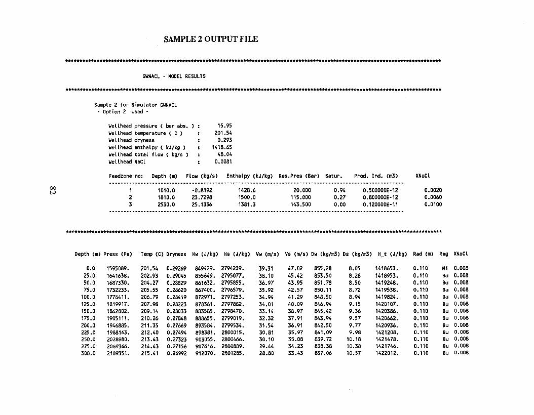
SAMPLE 2 OUTPUT FILE
**.'*******************************************************************************************************************************
GWNACL - MODEL RESULTS
**.,*******************************************************************************************************************************
Sample 2 for Simulator GWNACL• Option 2 used·
Wellhead pressure ( bar abs.Wellhead temperature ( C )Wellhead drynessWellhead enthalpy ( kJ/kg )Wellhead total flow ( kg/s )Wellhead HaCl
15.95201.540.293
1418.6548.04
0.0081
Feedzone no: Depth (m) Flow (kg/s) Enthalpy (kJ/kg) Res.Pres (Bar) Satur. Prod. Ind. (m3) XNaCl
00tv 1
23
1010.01810.02530.0
-0.819223.729825.1336
1428.61500.01381.3
20.000115.000143.500
0.940.270.00
0.500000E-120.800000E-12O. 120000E- 11
0.00200.00600.0100
**.r*******************************************************************************************************************************
Depth (m) Press (Pa) Temp (C) Dryness Hw (J/kg) Hs (J/kg) Vw (m/s) Vs (m/s) Dw (kg/m3) Ds (kg/m3) H_t (J/kg) Rad (m) Reg XNaCl
0.0 1595089. 201.54 0.29269 849429. 2794239. 39.31 47.02 855.28 8.05 1418653. 0.110 Mi 0.00825.0 1641638. 202.93 0.29045 855649. 2795077. 38.10 45.42 853.50 8.28 1418953. 0.110 Bu 0.00850.0 1687330. 204.27 0.28829 861632. 2795855. 36.97 43.95 851.78 8.50 1419248. 0.110 Bu 0.00875.0 1732233. 205.55 0.28620 867400. 2796579. 35.92 42.57 850.11 8.72 1419538. 0.110 Bu 0.008
100.0 1776411. 206.79 0.28419 872971. 2797253. 34.94 41.29 848.50 8.94 1419824. 0.110 Bu 0.008125.0 1819917. 207.98 0.28223 878361. 2797882. 34.01 40.09 846.94 9.15 1420107. 0.110 Bu 0.008150.0 1862802. 209.14 0.28033 883585. 2798470. 33.14 38.97 845.42 9.:56 1420386. 0.110 Bu 0.008175.0 1905111. 210.26 0.27848 888655. 2799019. 32.32 37.91 843.94 9.57 1420662. 0.110 Bu 0.008200.0 1946885. 211.35 0.27669 893584. 2799534. 31.54 36.91 842.50 9.77 1420936. 0.110 Bu 0.008225.0 1988163. 212.40 0.27494 898381. 2800015. 30.81 35.97 841.09 9.98 1421208. 0.110 Bu 0.008250.0 2028980. 213.43 0.27323 903055. 2800466. 30.10 35.08 839.72 10.18 1421478. 0.110 Bu 0.008275.0 2069366. 214.43 0.27156 907616. 2800889. 29.44 34.23 838.38 10.38 1421746. 0.110 Bu 0.008300.0 2109351. 215.41 0.26992 912070. 2'301285. 28.80 33.43 837.06 10.57 1422012. 0.110 Bu 0.008

315.0 2133161. 215.99 0.26896 914693. 2801510. 28.43 32.96 836.29 10.69 1422171. 0.110 Bu 0.008330.0 2156838. 216.56 0.26801 917282. 2801727. 28.07 32.51 835.52 10.81 1422330. 0.110 Bu 0.008345.0 2180391. 217.11 0.26707 919838. 2801936. 27.72 32.07 834.77 10.92 1422488. 0.110 Bu 0.008360.0 2203815. 217.67 0.26614 922361. 2802136. 27.39 31.65 834.02 11.04 1422645. 0.110 Bu 0.008375.0 2227125. 218.21 0.26522 924853. 2802329. 27.05 31.23 833.28 11.15 1422802. 0.110 Bu 0.008390.0 2250306. 218.75 0.26432 927313. 2802514. 26.73 30.83 832.55 11.27 1422958. 0.110 Bu 0.008405.0 2273382. 219.28 0.26342 929744. 2802692. 26.42 30.44 831.83 11.38 1423114. 0.110 Bu 0.008420.0 2296330. 219.80 0.26253 932145. 2802862. 26.11 30.05 831.11 11.49 1423269. 0.110 Bu 0.008435.0 2319181. 220.32 0.26166 934519. 2803026. 25.81 29.68 830.40 11.60 1423423. 0.110 Bu 0.008450.0 2341905. 220.83 0.26079 936864. 2803183. 25.52 29.32 829.70 11.72 1423581. 0.110 Bu 0.008465.0 2364539. 221.33 0.25993 939183. 2803334. 25.23 28.96 829.01 11.83 1423738. 0.110 Bu 0.008480.0 2387042. 221.83 0.25909 941475. 2803478. 24.95 28.62 828.33 11.94 1423894. 0.110 Bu 0.008495.0 2409462. 222.33 0.25825 943742. 2803616. 24.68 28.28 827.65 12.05 1424050. 0.110 Bu 0.008510.0 2431747. 222.81 0.25742 945982. 2803748. 24.41 27.95 826.98 12.16 1424204. 0.110 Bu 0.008525.0 2453957. 223.29 0.25660 948200. 2803874. 24.15 27.63 826.31 12.27 1424357. 0.110 Bu 0.008540.0 2476027. 223.77 0.25578 950391. 2803995. 23.90 27.32 825.66 12.38 1424509. 0.110 Bu 0.008555.0 2498026. 224.24 0.25498 952561. 2804110. 23.65 27.01 825.01 12.49 1424661. 0.110 Bu 0.008570.0 2519882. 224.70 0.25418 954704. 2804220. 23.41 26.71 824.36 12.60 1424810. 0.110 Bu 0.008585.0 2541673. 225.16 0.25339 956827. 2804325. 23.17 26.42 823.72 12.70 1424960. 0.110 Bu 0.008600.0 2563314. 225.61 0.25261 958924. 2804425. 22.93 26.13 823.09 12.81 1425107. 0.110 Bu 0.008615.0 2584895. 226.06 0.25183 961003. 2804519. 22.71 25.85 822.47 12.92 1425255. 0.110 Bu 0.008
00 630.0 2606320. 226.51 0.25106 963055. 2804609. 22.48 25.58 821.85 13.03 1425400. 0.110 Bu 0.008w 645.0 2627689. 226.95 0.25030 965090. 2804694. 22.26 25.31 821.24 13.13 1425545. 0.110 Bu 0.008660.0 2648895. 227.38 0.24955 967099. 2804775. 22.05 25.05 820.63 13.24 1425687. 0.110 Bu 0.008675.0 2670050. 227.81 0.24880 969091. 2804851. 21.84 24.79 820.03 13.34 1425829. 0.110 Bu 0.008690.0 2691033. 228.23 0.24806 971057. 2804923. 21.63 24.54 819.43 13.45 1425969. 0.110 Bu 0.008705.0 2711969. 228.65 0.24733 973008. 2804991. 21.43 24.30 818.84 13.55 1426109. 0.110 Bu 0.008720.0 2732725. 229.06 0.24660 974932. 2805054. 21.24 24.06 818.26 13.65 1426246. 0.110 Bu 0.008735.0 2753437. 229.47 0.24588 976842. 2805114. 21.04 23.82 817.68 13.76 1426383. 0.110 Bu 0.008750.0 2m961. 229.88 0.24517 978725. 2805170. 20.85 23.59 817.11 13.86 1426518. 0.110 Bu 0.008775.0 2808076. 230.55 0.24400 981835. 2805254. 20.54 23.22 816.17 14.03 1426744. 0.110 Bu 0.008800.0 2842083. 231.20 0.24283 984908. 2805329. 20.25 22.86 815.24 14.20 1426970. 0.110 Bu 0.008825.0 2875990. 231.85 0.24168 987948. 2805395. 19.95 22.51 814.31 14.37 1427195. 0.110 Bu 0.008850.0 2909804. 232.50 0.24054 990956. 2805451. 19.67 22.16 813.40 14.54 1427420. 0.110 Bu 0.008875.0 2943534. 233.13 0.23941 993932. 2805499. 19.39 21.83 812.49 14.71 1427644. 0.110 Bu 0.008900.0 2977188. 233.76 0.23829 996879. 2805538. 19.12 21.50 811.59 14.87 1427868. 0.110 Bu 0.008910.0 2990628. 234.01 0.23785 998050. 2805551. 19.01 21.38 811.24 14.94 1427956. 0.110 Bu 0.008935.0 3073821. 235.54 0.23477 1005222. 2805604. 29.58 32.78 809.04 15.36 1427900. 0.087 Bu 0.008960.0 3127326. 236.50 0.23296 1009764. 2805613. 28.93 32.02 807.65 15.63 1428132. 0.087 Bu 0.008985.0 3180372. 237.45 0.23119 1014216. 2805602. 28.32 31.30 806.28 15.89 1428364. 0.087 Bu 0.008
1010.0 3232992. 238.37 0.22944 1018583. 2805573. 27.72 30.61 804.94 16.16 1428594. 0.087 Bu 0.0081010.0 3232992. 238.37 0.229/.4 1018583. 2805573. 28.22 31.13 804.94 16.16 1428594. 0.087 Bu 0.0081035.0 3286181. 239.29 0.22769 1022950. 2805527. 27.63 30.45 803.60 16.43 1428824. 0.087 Bu 0.008
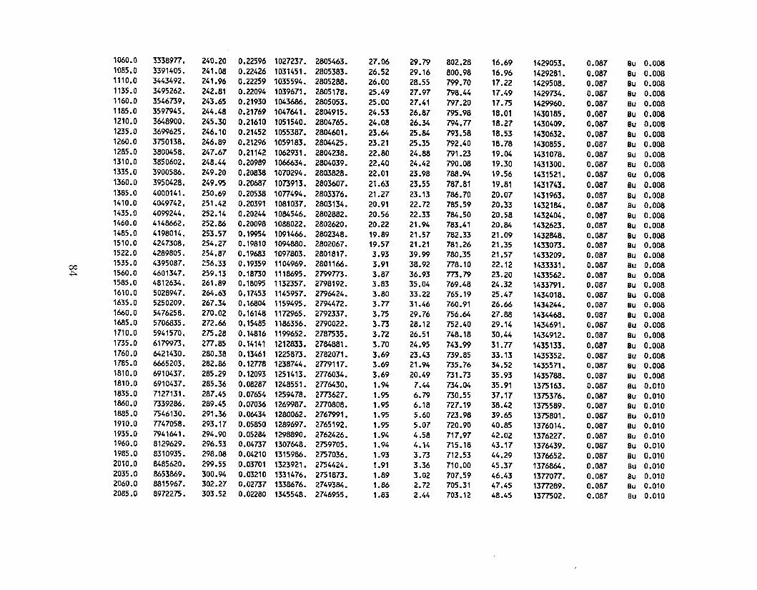
1060.0 3338977. 240.20 0.22596 1027237. 2805463. 27.06 29.79 802.28 16.69 1429053. 0.087 Bu 0.0081085.0 3391405. 241. OS 0.22426 1031451. 2805383. 26.52 29.16 800.98 16.96 1429281. 0.087 Bu 0.0081110.0 3443492. 241.96 0.22259 1035594. 2805288. 26.00 28.55 799.70 17.22 1429508. 0.087 Bu 0.0081135.0 3495262. 242.81 0.22094 1039671- 2805178. 25.49 27.97 798.44 17.49 1429734. 0.OS7 Bu O.OOS1160.0 3546739. 243.65 0.21930 1043686. 2805053. 25.00 27.41 797.20 17.75 1429960. 0.087 Bu 0.0081185.0 3597945. 244.48 0.21769 1047641. 2804915. 24.53 26.87 795.98 18.01 1430185. 0.087 Bu 0.0081210.0 3648900. 245.30 0.21610 1051540. 2804765. 24.08 26.34 794.77 18.27 1430409. 0.087 Bu 0.0081235.0 3699625. 246.10 0.21452 1055387. 2804601. 23.64 25.84 793.58 18.53 1430632. 0.087 Bu 0.0081260.0 3750138. 246.89 0.21296 1059183. 2804425. 23.21 25.35 792.40 18.78 1430855. 0.087 Bu 0.0081285.0 3800458. 247.67 0.21142 1062931. 2804238. 22.80 24.88 791.23 19.04 1431078. 0.087 Bu 0.0081310.0 3850602. 248.44 0.20989 1066634. 2804039. 22.40 24.42 790.08 19.30 1431300. 0.087 Bu 0.0081335.0 3900586. 249.20 0.20838 1070294. 2803828. 22.01 23.98 788.94 19.56 1431521. 0.087 Bu 0.0081360.0 3950428. 249.95 0.20687 1073913. 2803607. 21.63 23.55 787.81 19.81 1431743. 0.OS7 Bu O.OOS1385.0 4000141. 250.69 0.20538 1077494. 2803376. 21.27 23.13 786.70 20.07 1431963. 0.087 Bu 0.0081410.0 4049742. 251.42 0.20391 1081037. 2803134. 20.91 22.72 785.59 20.33 1432184. 0.087 Bu 0.0081435.0 4099244. 252.14 0.20244 1084546. 2802882. 20.56 22.33 784.50 20.58 1432404. 0.087 Bu 0.0081460.0 4148662. 252.86 0.20098 1088022. 2802620. 20.22 21.94 783.41 20.84 1432623. 0.087 Bu 0.0081485.0 4198014. 253.57 0.19954 1091466. 2802348. 19.89 21.57 782.33 21.09 1432848. 0.087 Bu 0.0081510.0 4247308. 254.27 0.19810 1094880. 2802067. 19.57 21.21 781.26 21.35 1433073. 0.087 Bu 0.0081522.0 4289805. 254.87 0.19683 1097803. 2801817. 3.93 39.99 780.35 21.57 1433209. 0.087 Bu O.OOS1535.0 4395087. 256.33 0.19359 1104969. 2801166. 3.91 38.92 778.10 22.12 1433331. 0.087 Bu 0.008001560.0 4601347. 259.13 0.18730 1118695. 2799m. 3.87 36.93 m.79 23.20 1433562. 0.087 Bu 0.008+::-1585.0 4812634. 261.89 0.18095 1132357. 2798192. 3.83 35.04 769.48 24.32 1433791. 0.087 Bu 0.0081610.0 5028947. 264.63 0.17453 1145957. 2796424. 3.80 33.22 765.19 25.47 1434018. 0.087 Bu 0.0081635.0 5250209. 267.34 0.16804 1159495. 2794472. 3.77 31.46 760.91 26.66 1434244. 0.087 Bu 0.0081660.0 5476258. 270.02 0.16148 1172965. 2792337. 3.75 29.76 756.64 27.88 1434468. 0.087 Bu 0.0081685.0 5706835. 272.66 0.15485 1186356. 2790022. 3.73 28.12 752.40 29.14 1434691. 0.087 Bu 0.0081710.0 5941570. 275.28 0.14816 1199652. 2787535. 3.72 26.51 748.18 30.44 1434912. 0.087 Bu 0.0081735.0 6179973. 277.85 0.14141 1212833. 2784881. 3.70 24.95 743.99 31.77 1435133. 0.OS7 Bu 0.0081760.0 6421430. 280.38 0.13461 1225873. 2782071. 3.69 23.43 739.85 33.13 1435352. 0.087 Bu 0.0081785.0 6665203. 282.86 0.12778 1238744. 2779117. 3.69 21.94 735.76 34.52 1435571. 0.087 Bu 0.0081810.0 6910437. 285.29 0.12093 1251413. 2776034. 3.69 20.49 731.73 35.93 1435788. 0.087 Bu 0.0081810.0 6910437. 285.36 0.08287 1248551. 2776430. 1.94 7.44 734.04 35.91 1375163. 0.087 Bu 0.0101835.0 7127131- 287.45 0.07654 1259478. 2m627. 1.95 6.79 730.55 37.17 1375376. 0.087 Bu 0.0101860.0 7339286. 289.45 0.07036 1269987. 2770808. 1.95 6.18 727.19 38.42 1375589. 0.087 Bu 0.0101885.0 7546130. 291.36 0.06434 1280062. 2767991. 1.95 5.60 723.98 39.65 1375801. 0.087 Bu 0.0101910.0 7747058. 293.17 0.05850 1289697. 2765192. 1.95 5.07 720.90 40.85 1376014. 0.087 Bu 0.0101935.0 7941641. 294.90 0.05284 1298890. 2762426. 1.94 4.58 717.97 42.02 1376227. 0.087 Bu 0.0101960.0 8129629. 296.53 0.04737 1307648. 2759705. 1.94 4.14 715.18 43.17 1376439. 0.087 Bu 0.0101985.0 8310935. 298.08 0.04210 1315986. 2757036. 1.93 3.73 712.53 44.29 1376652. 0.087 Bu 0.0102010.0 8485620. 299.55 0.03701 1323921. 2754424. 1.91 3.36 710.00 45.37 1376864. 0.087 Bu 0.0102035.0 8653869. 300.94 0.03210 1331476. 2751873. 1.89 3.02 707.59 46.43 1377077. 0.087 Bu 0.0102060.0 8815967. 302.27 0.02737 1338676. 2749384. 1.86 2.72 705.31 47.45 1377289. 0.087 Bu 0.0102085.0 8972275. 303.52 0.02280 1345548. 2746955. 1.83 2.44 703.12 48.45 13m02. 0.087 Bu 0.010
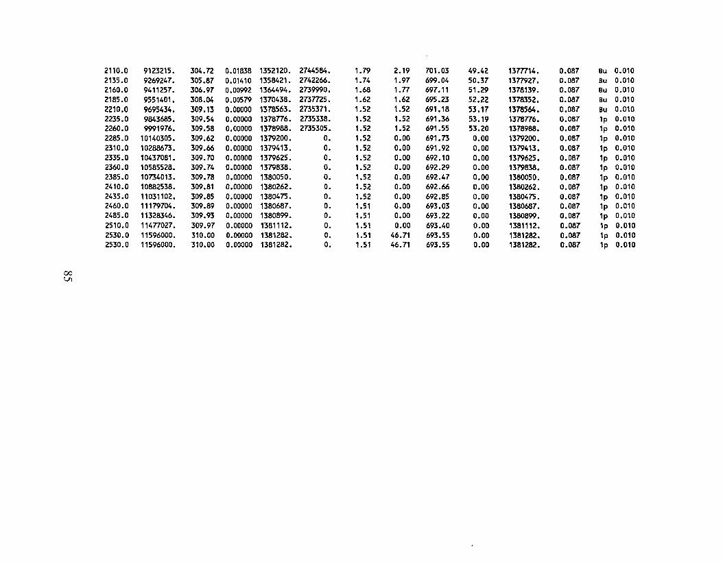
2110.0 9123215. 304.n 0.01838 1352120. 2744584. 1.79 2.19 701.03 49.42 13m14. 0.087 Bu 0.0102135.0 9269247. 305.87 0.01410 1358421. 2742266. 1.74 1.97 699.04 50.37 1377927. 0.087 Bu 0.0102160.0 9411257. 306.97 0.00992 1364494. 2739990. 1.68 1.n 697.11 51.29 1378139. 0.087 Bu 0.0102185.0 9551401. 308.04 0.00579 1370438. 273n25. 1.62 1.62 695.23 52.22 1378352. 0.087 Bu 0.0102210.0 9695434. 309.13 0.00000 1378563. 2735371. 1.52 1.52 691.18 53.17 1378564. 0.087 Bu 0.0102235.0 9843685. 309.54 0.00000 1378n6. 2735338. 1.52 1.52 691.36 53.19 1378n6. 0.087 1p 0.0102260.0 9991976. 309.58 0.00000 1378988. 2735305. 1.52 1.52 691.55 53.20 1378988. 0.087 1p 0.0102285.0 10140305. 309.62 0.00000 1379200. O. 1.52 0.00 691.73 0.00 1379200. 0.087 1p 0.0102310.0 10288673. 309.66 0.00000 1379413. O. 1.52 0.00 691.92 0.00 1379413. 0.087 1p 0.0102335.0 10437081. 309.70 0.00000 1379625. O. 1.52 0.00 692.10 0.00 1379625. 0.087 1p 0.0102360.0 10585528. 309.74 0.00000 1379838. O. 1.52 0.00 692.29 0.00 1379838. 0.087 1p 0.0102385.0 10734013. 309.78 0.00000 1380050. O. 1.52 0.00 692.47 0.00 1380050. 0.087 1p 0.0102410.0 10882538. 309.81 0.00000 1380262. O. 1.52 0.00 692.66 0.00 1380262. 0.087 1p 0.0102435.0 11031102. 309.85 0.00000 1380475. O. 1.52 0.00 692.85 0.00 1380475. 0.087 1p 0.0102460.0 11179704. 309.89 0.00000 1380687. O. 1.51 0.00 693.03 0.00 1380687. 0.087 1p 0.0102485.0 11328346. 309.93 0.00000 1380899. O. 1.51 0.00 693.22 0.00 1380899. 0.087 1p 0.0102510.0 114n027. 309.97 0.00000 1381112. O. 1.51 0.00 693.40 0.00 1381112. 0.087 1p 0.0102530.0 11596000. 310.00 0.00000 1381282. O. 1.51 46.71 693.55 0.00 1381282. 0.087 1p 0.0102530.0 11596000. 310.00 0.00000 1381282. O. 1.51 46.71 693.55 0.00 1381282. 0.087 1p 0.010
00VI
APPENDIXC
(SAMPLE RUNS FOR HOLA)
86

SAMPLE 1 INPUT FILE
Sample 1 for Simulator HOL~
- Option 1 used-- The well is producing two-phase fluid at the wellhead -
0.7000E+061. 3000E+06100.0000
2530.0002.0002800.0001000.0006.0480E+0520
300.0 0.1102 4.6E-5 25.0 90.030.0 0.1102 4.6E-5 15.0 88.030.0 0.1102 4.6E-5 15.0 86.030.0 0.1102 4.6E-5 15.0 84.030.0 0.1102 4.6E-5 15.0 82.030.0 0.1102 4.6E-5 15.0 80.030.0 0.1102 4.6E-5 15.0 78.030.0 0.1102 4.6E-5 15.0 76.030.0 0.1102 4.6E-5 15.0 74.030.0 0.1102 4.6E-5 15.0 72.030.0 0.1102 4.6E-5 15.0 70.030.0 0.1102 4.6E-5 15.0 68.030.0 0.1102 4.6E-5 15.0 66.030.0 0.1102 4.6E-5 15.0 64.030.0 0.1102 4.6E-5 15.0 62.030.0 0.1102 4.6E-5 15.0 60.0
150.0 0.1102 4.6E-5 25.0 60.010.0 0.1102 4.6E-5 10.0 60.0
1600.0 0.0873 1. 5E-5 25.0 60.020.0 0.0873 1.5E-5 20.0 60.0
40.0 25.00
1000.0 260.002000.0 310.002500.0 330.00
31110.0 -10.00 1.0000E+061810.0 40.00 1.5000E+06
SAMPLE 1 HOLA.LOG FILE
Two phase to water phasePressure X2 Depth
0.834715E+07 -0.00033092 1235.0
87
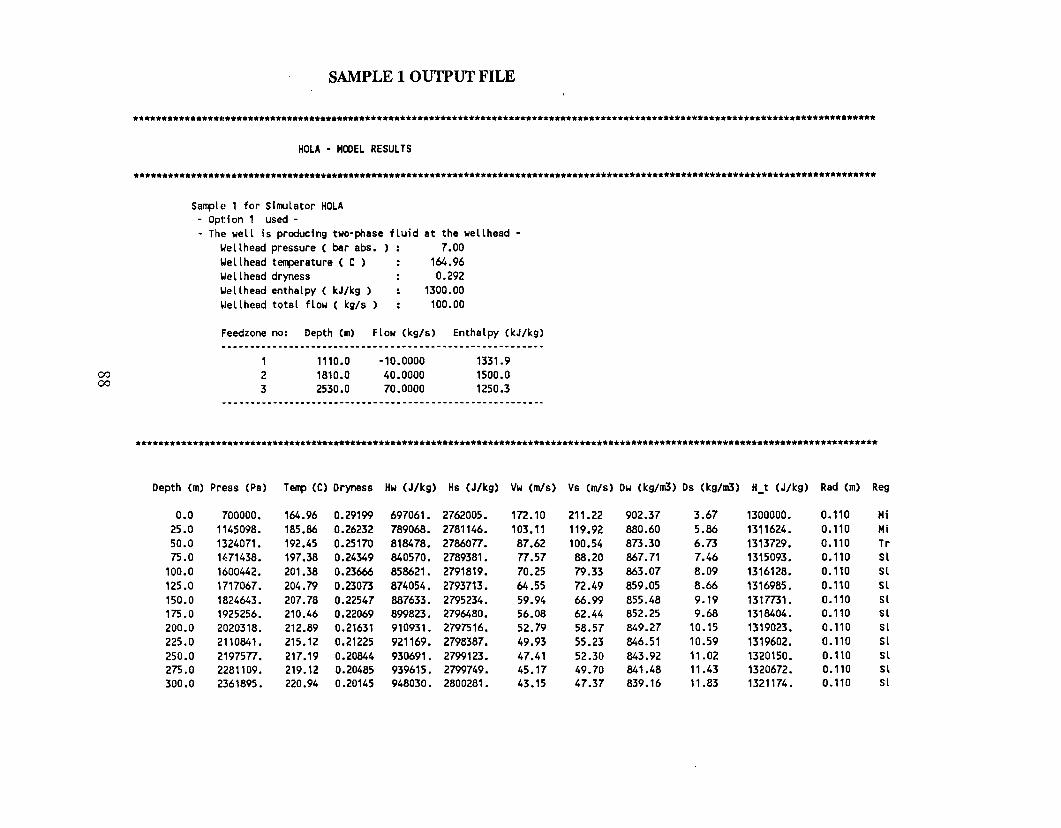
SAMPLE 1 OUTPUT FILE
**********************************************************************************************************************************
HOLA - HODEL RESULTS
**********************************************************************************************************************************
Sample 1 for Simulator HOLA- Option 1 used-• The well is producing two-phase fluid at the wellhead -
~Ie II head pressure ( bar abs. ) : 7.00Wellhead temperature ( C ) : 164.96~Iellhead dryness : 0.292~ellhead enthalpy ( kJ/kg) : 1300.00~ellhead total flow ( kg/s): 100.00
Feedzone no: Depth (m) Flow (kg/s) Enthalpy (kJ/kg)
0000
123
1110.01810.02530.0
-10.000040.000070.0000
1331.91500.01250.3
**********************************************************************************************************************************
Depth (m) Press (Pa) Temp (C) Dryness Hw (J/kg) Hs (J/kg) Vw (m/s) Vs (m/s) Ow (kg/m3) Os (kg/m3) H_t (J/kg) Rad (m) Reg
0.0 700000. 164.96 0.29199 697061. 2762005. 1n.10 211.22 902.37 3.67 1300000. 0.110 Hi25.0 1145098. 185.86 0.26232 789068. 2781146. 103.11 119.92 880.60 5.86 1311624. 0.110 Hi50.0 1324071. 192.45 0.25170 818478. 2786077. 87.62 100.54 873.30 6.73 1313n9. 0.110 Tr75.0 11,71438. 197.38 0.24349 840570. 2789381. 77.57 88.20 867.71 7.46 1315093. 0.110 Sl
100.0 1600442. 201.38 0.23666 858621. 2791819. 70.25 79.33 863.07 8.09 1316128. 0.110 5l125.0 1717067. 204.79 0.23073 874054. 2793713. 64.55 n.49 859.05 8.66 1316985. 0.110 Sl150.0 1824643. 207.78 0.22547 887633. 2795234. 59.94 66.99 855.48 9.19 131m1. 0.110 5l175 .0 1925256. 210.46 0.22069 899823. 2796480. 56.08 62.44 852.25 9.68 1318404. 0.110 5l200.0 2020318. 212.89 0.21631 910931. 2797516. 52.79 58.57 849.27 10.15 1319023. 0.110 5l225.0 2110841. 215.12 0.21225 921169. 2798387. 49.93 55.23 846.51 10.59 1319602. 0.110 Sl250.0 2197577. 217.19 0.20844 930691. 2799123. 47.41 52.30 843.92 11.02 1320150. 0.110 5l275.0 2281109. 219.12 0.20485 939615. 2799749. 45.17 49.70 841.48 11.43 1320672. 0.110 5l300.0 2361895. 220.94 0.20145 948030. 2800281. 43.15 47.37 839.16 11.83 1321174. 0.110 5l
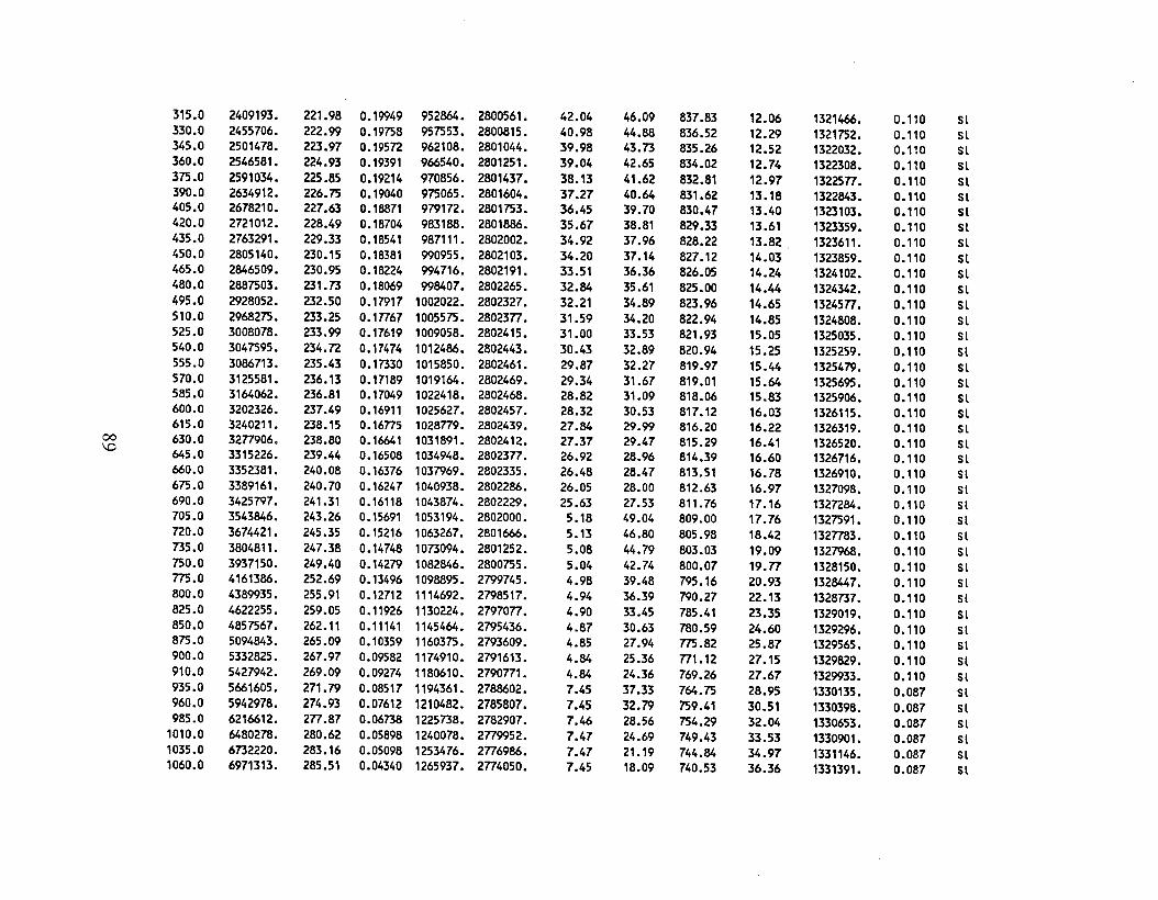
315.0 2409193. 221.98 0.19949 952864. 2800561. 42.04 46.09 837.83 12.06 1321466. 0.110 Sl330.0 2455706. 222.99 0.19758 957553. 2800815. 40.98 44.88 836.52 12.29 1321752. 0.110 Sl345.0 2501478. 223.97 0.195n 962108. 2801044. 39.98 43.73 835.26 12.52 1322032. 0.110 Sl360.0 2546581. 224.93 0.19391 966540. 2801251. 39.04 42.65 834.02 12.74 1322308. 0.110 Sl375.0 2591034. 225.85 0.19214 970856. 2801437. 38.13 41.62 832.81 12.97 1322577. 0.110 Sl390.0 2634912. 226.75 0.19040 975065. 2801604. 37.27 40.64 831.62 13.18 1322843. 0.110 Sl405.0 2678210. 227.63 0.18871 979172. 2801753. 36.45 39.70 830.47 13.40 1323103. 0.110 Sl420.0 2721012. 228.49 0.18704 983188. 2801886. 35.67 38.81 829.33 13.61 1323359. 0.110 Sl435.0 2763291. 229.33 0.18541 987111. 2802002. 34.92 37.96 828.22 13.82 1323611. 0.110 Sl450.0 2805140. 230.15 0.18381 990955. 2802103. 34.20 37.14 827.12 14.03 1323859. 0.110 Sl465.0 2846509. 230.95 0.18224 994716. 2802191. 33.51 36.36 826.05 14.24 1324102. 0.110 Sl480.0 2887503. 231.73 0.18069 998407. 2802265. 32.84 35.61 825.00 14.44 1324342. 0.110 Sl495.0 2928052. 232.50 0.17917 1002022. 2802327. 32.21 34.89 823.96 14.65 1324577. 0.110 Sl510.0 2968275. 233.25 0.1n67 1005575. 2802377. 31.59 34.20 822.94 14.85 1324808. 0.110 Sl525.0 3008078. 233.99 0.17619 1009058. 2802415. 31.00 33.53 821.93 15.05 1325035. 0.110 Sl540.0 3047595. 234.72 0.17474 1012486. 2802443. 30.43 32.89 820.94 15.25 1325259. 0.110 Sl555.0 3086713. 235.43 0.17330 1015850. 2802461. 29.87 32.27 819.97 15.44 1325479. 0.110 Sl570.0 3125581. 236.13 0.17189 1019164. 2802469. 29.34 31.67 819.01 15.64 1325695. 0.110 Sl585.0 3164062. 236.81 0.17049 1022418. 2802468. 28.82 31.09 818.06 15.83 1325906. 0.110 Sl600.0 3202326. 237.49 0.16911 1025627. 2802457. 28.32 30.53 817.12 16.03 1326115. 0.110 Sl615.0 3240211. 238.15 0.16775 1028779. 2802439. 27.84 29.99 816.20 16.22 1326319. 0.110 Sl
00 630.0 3277906. 238.80 0.16641 1031891. 2802412. 27.37 29.47 815.29 16.41 1326520. 0.110 Sl\0 645.0 3315226. 239.44 0.16508 1034948. 2802377. 26.92 28.96 814.39 16.60 1326716. 0.110 Sl660.0 3352381. 240.08 0.16376 1037969. 2802335. 26.48 28.47 813.51 16.78 1326910. 0.110 Sl675.0 3389161. 240.70 0.16247 1040938. 2802286. 26.05 28.00 812.63 16.97 1327098. 0.110 Sl690.0 3425797. 241.31 0.16118 1043874. 2802229. 25.63 27.53 811. 76 17.16 1327284. 0.110 Sl705.0 3543846. 243.26 0.15691 1053194. 2802000. 5.18 49.04 809.00 17.76 1327591. 0.110 Sl720.0 3674421. 245.35 0.15216 1063267. 2801666. 5.13 46.80 805.98 18.42 1327783. 0.110 Sl735.0 3804811. 247.38 0.14748 1073094. 2801252. 5.08 44.79 803.03 19.09 1327968. 0.110 Sl750.0 3937150. 249.40 0.14279 1082846. 2800755. 5.04 42.74 800.07 19.77 1328150. 0.110 Sl775.0 4161386. 252.69 0.13496 1098895. 2799745. 4.98 39.48 795.16 20.93 1328447. 0.110 Sl800.0 4389935. 255.91 0.12712 1114692. 2798517. 4.94 36.39 790.27 22.13 1328737. 0.110 Sl825.0 4622255. 259.05 0.11926 1130224. 2797077. 4.90 33.45 785.41 23.35 1329019. 0.110 Sl850.0 4857567. 262.11 0.11141 1145464. 2795436. 4.87 30.63 780.59 24.60 1329296. 0.110 Sl875.0 5094843. 265.09 0.10359 1160375. 2793609. 4.85 27.94 775.82 25.87 1329565. 0.110 Sl900.0 5332825. 267.97 0.09582 1174910. 2791613. 4.84 25.36 771.12 27.15 1329829. 0.110 Sl910.0 5427942. 269.09 0.09274 1180610. 2790771. 4.84 24.36 769.26 27.67 1329933. 0.110 Sl935.0 5661605. 271.79 0.08517 1194361. 2788602. 7.45 37.33 764.75 28.95 1330135. 0.087 Sl960.0 5942978. 274.93 0.07612 1210482. 2785807. 7.45 32.79 759.41 30.51 1330398. 0.087 Sl985.0 6216612. 277.87 0.06738 1225738. 2782907. 7.46 28.56 754.29 32.04 1330653. 0.087 Sl
1010.0 6480278. 280.62 0.05898 1240078. 2779952. 7.47 24.69 749.43 33.53 1330901. 0.087 Sl1035.0 6732220. 283.16 0.05098 1253476. 2776986. 7.47 21.19 744.84 34.97 1331146. 0.087 Sl1060.0 6971313. 285.51 0.04340 1265937. 2774050. 7.45 18.09 740.53 36.36 1331391. 0.087 Sl
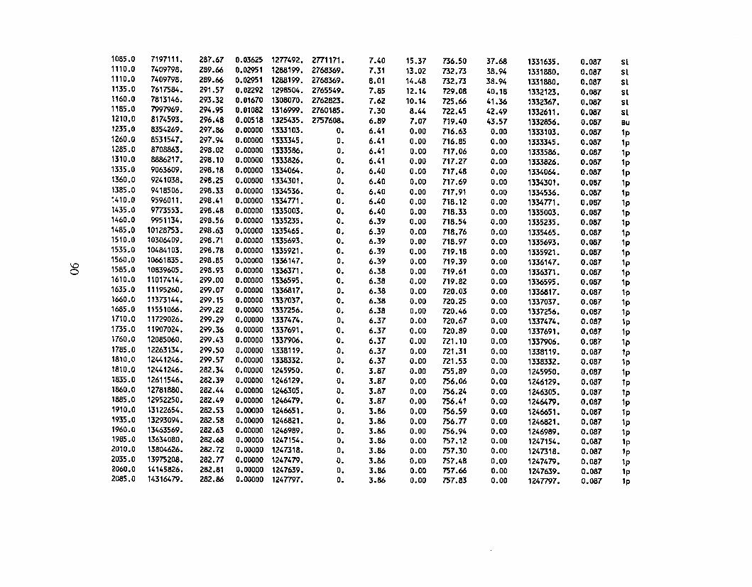
1085.0 7197111- 287.67 0.03625 12n492. 2n1171. 7.40 15.37 736.50 37.68 1331635. 0.087 Sl1110.0 7409798. 289.66 0.02951 1288199. 2768369. 7.31 13.02 732.73 38.94 1331880. 0.087 Sl1110.0 7409798. 289.66 0.02951 1288199. 2768369. 8.01 14.48 732.73 38.94 1331880. 0.087 Sl1135.0 7617584. 291.57 0.02292 1298504. 2765549. 7.85 12.14 729.08 40.18 1332123. 0.087 Sl1160.0 7813146. 293.32 0.01670 1308070. 2762823. 7.62 10.14 725.66 41.36 1332367. 0.087 Sl1185.0 7997969. 294.95 0.01082 1316999. 2760185. 7.30 8.44 722.45 42.49 1332611. 0.087 Sl1210.0 8174593. 296.48 0.00518 1325435. 2757608. 6.89 7.07 719.40 43.57 1332856. 0.087 Bu1235.0 8354269. 297.86 0.00000 1333103. O. 6.41 0.00 716.63 0.00 1333103. 0.087 1p1260.0 8531547. 297.94 0.00000 1333345. O. 6.41 0.00 716.85 0.00 1333345. 0.087 1p1285.0 8708863. 298.02 0.00000 1333586. O. 6.41 0.00 717.06 0.00 1333586. 0.087 1p1310.0 8886217. 298.10 0.00000 1333826. O. 6.41 0.00 717.27 0.00 1333826. 0.087 1p1335.0 9063609. 298.18 0.00000 1334064. O. 6.40 0.00 717.48 0.00 1334064. 0.087 1p1360.0 9241038. 298.25 0.00000 1334301. O. 6.40 0.00 717.69 0.00 1334301. 0.087 1p1385.0 9418506. 298.33 0.00000 1334536. O. 6.40 0.00 717.91 0.00 1334536. 0.087 1p~410.0 9596011. 298.41 0.00000 1334n1. O. 6.40 0.00 718.12 0.00 1334n1. 0.087 1p1435.0 9m553. 298.48 0.00000 1335003. O. 6.40 0.00 718.33 0.00 1335003. 0.087 1p1460.0 9951134. 298.56 0.00000 1335235. O. 6.39 0.00 718.54 0.00 1335235. 0.087 1p1485.0 10128753. 298.63 0.00000 1335465. O. 6.39 0.00 718.76 0.00 1335465. 0.087 1p1510.0 10306409. 298.71 0.00000 1335693. O. 6.39 0.00 718.97 0.00 1335693. 0.087 1p1535.0 10484103. 298.78 0.00000 1335921. O. 6.39 0.00 719.18 0.00 1335921. 0.087 1p1560.0 10661835. 298.85 0.00000 1336147. O. 6.39 0.00 719.39 0.00 1336147. 0.087 1p\D 1585.0 10839605. 298.93 0.00000 1336371. O. 6.38 0.00 719.61 0.00 1336371. 0.087 1p01610.0 11017414. 299.00 0.00000 1336595. O. 6.38 0.00 719.82 0.00 1336595. 0.087 1p1635.0 11195260. 299.07 0.00000 1336817. O. 6.38 0.00 720.03 0.00 1336817. 0.087 1p1660.0 11373144. 299.15 0.00000 1337037. O. 6.38 0.00 720.25 0.00 1337037. 0.087 1p1685.0 11551066. 299.22 0.00000 1337256. O. 6.38 0.00 720.46 0.00 1337256. 0.087 1p1710.0 11729026. 299.29 0.00000 1337474. O. 6.37 0.00 720.67 0.00 1337474. 0.087 1p1735.0 11907024. 299.36 0.00000 1337691. O. 6.37 0.00 720.89 0.00 1337691. 0.087 1p1760.0 12085060. 299.43 0.00000 1337906. O. 6.37 0.00 721.10 0.00 1337906. 0.087 1p1785.0 12263134. 299.50 0.00000 1338119. O. 6.37 0.00 721.31 0.00 1338119. 0.087 1p1810.0 12441246. 299.57 0.00000 1338332. O. 6.37 0.00 721.53 0.00 1338332. 0.087 1p1810.0 12441246. 282.34 0.00000 1245950. O. 3.87 0.00 755.89 0.00 1245950. 0.087 1p1835.0 12611546. 282.39 0.00000 1246129. O. 3.87 0.00 756.06 0.00 1246129. 0.087 1p1860.0 12781880. 282.44 0.00000 1246305. O. 3.87 0.00 756.24 0.00 1246305. 0.087 1p1885.0 12952250. 282.49 0.00000 1246479. O. 3.87 0.00 756.41 0.00 1246479. 0.087 1p1910.0 13122654. 282.53 0.00000 1246651. O. 3.86 0.00 756.59 0.00 1246651. 0.087 1p1935.0 13293094. 282.58 0.00000 1246821. O. 3.86 0.00 756.n 0.00 1246821- 0.087 1p1960.0 13463569. 282.63 0.00000 1246989. O. 3.86 0.00 756.94 0.00 1246989. 0.087 1p1985.0 13634080. 282.68 0.00000 1247154. O. 3.86 0.00 757.12 0.00 1247154. 0.087 1p2010.0 13804626. 282.72 0.00000 1247318. O. 3.86 0.00 757.30 0.00 1247318. 0.087 1p2035.0 13975208. 282.n 0.00000 1247479. O. 3.86 0.00 757.48 0.00 1247479. 0.087 1p2060.0 14145826. 282.81 0.00000 1247639. O. 3.86 0.00 757.66 0.00 1247639. 0.087 1p2085.0 14316479. 282.86 0.00000 124n97. O. 3.86 0.00 757.83 0.00 1247797. 0.087 1p
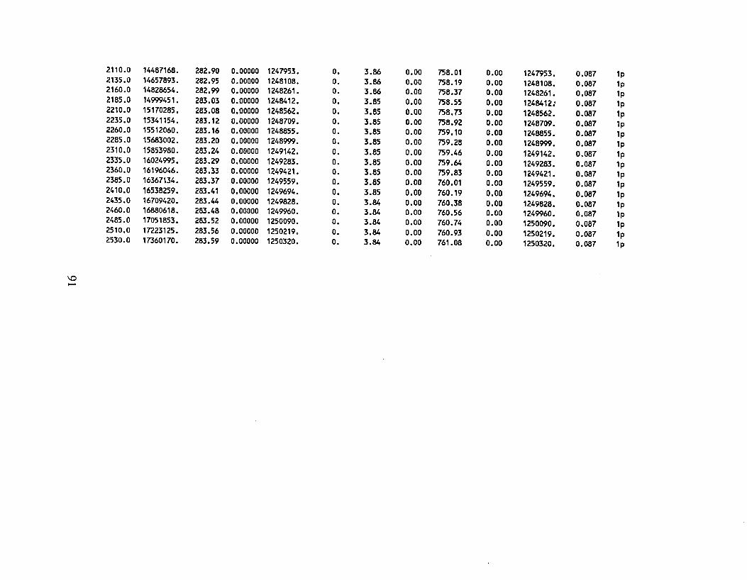
\0I-'
2110.0 14487168. 282.90 0.00000 1247953. O. 3.86 0.00 758.01 0.00 1247953. 0.087 1p2135.0 14657893. 282.95 0.00000 1248108. O. 3.86 0.00 758.19 0.00 1248108. 0.087 1p2160.0 14828654. 282.99 0.00000 1248261- O. 3.86 0.00 758.37 0.00 1248261. 0.087 1p2185.0 14999451. 283.03 0.00000 1248412. O. 3.85 0.00 758.55 0.00 1248412: 0.087 1p2210.0 15170285. 283.08 0.00000 1248562. O. 3.85 0.00 758.73 0.00 1248562. 0.087 1p2235.0 15341154. 283.12 0.00000 1248709. O. 3.85 0.00 758.92 0.00 1248709. 0.087 1p2260.0 15512060. 283.16 0.00000 1248855. O. 3.85 0.00 759.10 0.00 1248855. 0.087 1p2285.0 15683002. 283.20 0.00000 1248999. O. 3.85 0.00 759.28 0.00 1248999. 0.087 1p2310.0 15853980. 283.24 0.00000 1249142. O. 3.85 0.00 759.46 0.00 1249142. 0.087 1p2335.0 16024995. 283.29 0.00000 1249283. O. 3.85 0.00 759.64 0.00 1249283. 0.087 1p2360.0 16196046. 283.33 0.00000 1249421. O. 3.85 0.00 759.83 0.00 1249421- 0.087 1p2385.0 16367134. 283.37 0.00000 1249559. O. 3.85 0.00 760.01 0.00 1249559. 0.087 1p2410.0 16538259. 283.41 0.00000 1249694. O. 3.85 0.00 760.19 0.00 1249694. 0.087 1p2435.0 16709420. 283.44 0.00000 1249828. O. 3.84 0.00 760.38 0.00 1249828. 0.087 1p2460.0 16880618. 283.48 0.00000 1249960. O. 3.84 0.00 760.56 0.00 1249960. 0.087 1p2485.0 17051853. 283.52 0.00000 1250090. O. 3.84 0.00 760.74 0.00 1250090. 0.087 1p2510.0 17223125. 283.56 0.00000 1250219. O. 3.84 0.00 760.93 0.00 1250219. 0.087 1p2530.0 17360170. 283.59 0.00000 1250320. O. 3.84 0.00 761.08 0.00 1250320. 0.087 1p
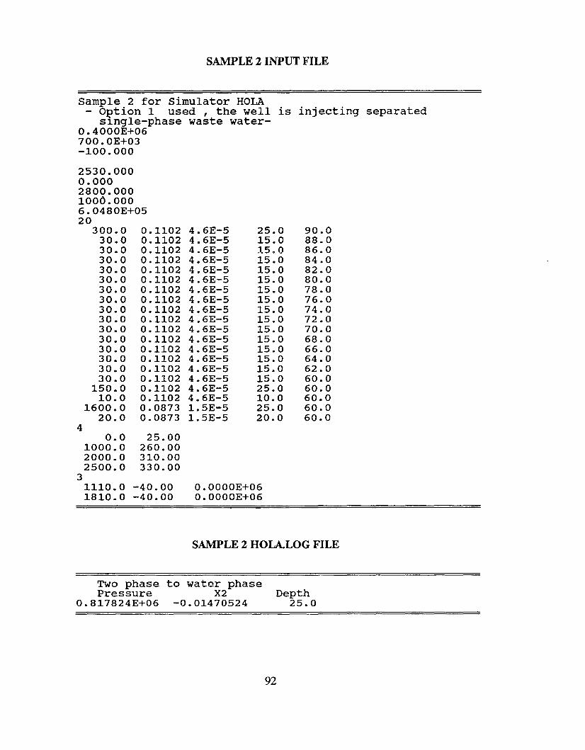
SAMPLE 2 INPUT FILE
Sample 2 for Simulator HOLA- o~tion 1 used, the well is injecting separated
s1ngle-phase waste water0.4000E+06700.0E+03-100.000
2530.0000.0002800.0001000.0006.0480E+OS20
300.0 0.1102 4.6E-5 2S.0 90.030.0 0.1102 4.6E-5 lS.0 88.030.0 0.1102 4.6E-S lS.0 86.030.0 0.1102 4.6E-5 15.0 84.030.0 0.1102 4.6E-S 1S.0 82.030.0 0.1102 4.6E-S 15.0 80.030.0 0.1102 4.6E-S lS.0 78.030.0 0.1102 4.6E-S lS.0 76.030.0 0.1102 4.6E-5 15.0 74.030.0 0.1102 4.6E-5 lS.0 72.030.0 0.1102 4.6E-S lS.0 70.030.0 0.1102 4.6E-S lS.0 68.030.0 0.1102 4.6E-S lS.0 66.030.0 0.1102 4.6E-S lS.0 64.030.0 0.1102 4.6E-S 15.0 62.030.0 0.1102 4.6E-S 15.0 60.0
lS0.0 0.1102 4.6E-S 2S.0 60.010.0 0.1102 4.6E-S 10.0 60.0
1600.0 0.0873 1.SE-S 2S.0 60.020.0 0.0873 1. SE-S 20.0 60.0
40.0 2S.00
1000.0 260.002000.0 310.002500.0 330.00
31110.0 -40.00 0.0000E+061810.0 -40.00 0.0000E+06
SAMPLE 2 HOLA.LOG FILE
Two phase to water phasePressure X2 Depth
0.817824E+06 -0.01470524 2S.0
92
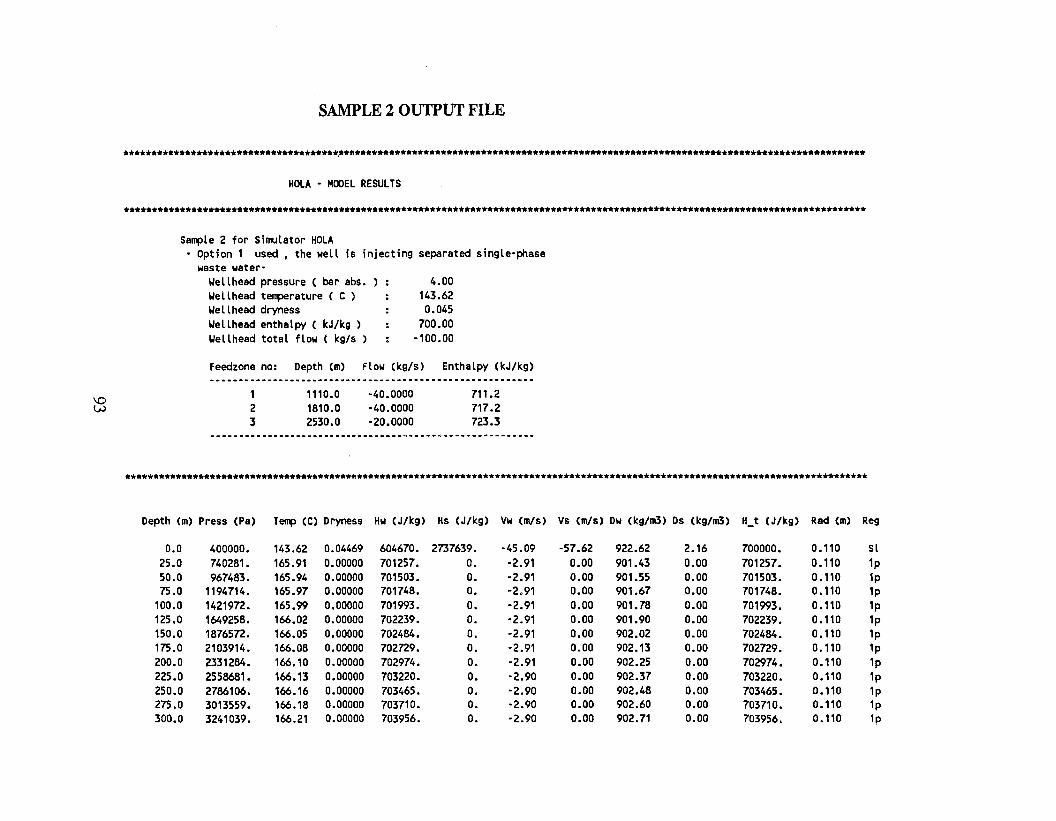
4.00143.620.045
700.00-100.00
SAMPLE 2 OUTPUT FILE
**************************************~*******************************************************************************************
HOLA - MODEL RESULTS
**********************************************************************************************************************************
Sample 2 for Simulator HOLAOption 1 used, the well is injecting separated single-phasewaste water-~ellhead pressure ( bar abs.~ellhead temperature ( C )~ellhead dryness~ellhead enthalpy ( kJ/kg )~ellhead total flow ( kg/s )
Feedzone no: Depth (m) Flow (kg/s) Enthalpy (kJ/kg)
\0V.)
123
1110.01810.02530.0
-40.0000-40.0000-20.0000
711.2717.2723.3
******************.*********************************************.***************************************************************.*
Depth (m) Press (Pa) Temp (C) Dryness Hw (J/kg) Hs (J/kg) Vw (m!s) VS (m/s) Ow (kg/m3) Os (kg/m3) H_t (J/kg) Rad (m) Reg
0.0 400000. 143.62 0.04469 604670. 2737639. -45.09 -57.62 922.62 2.16 700000. 0.110 Sl25.0 740281. 165.91 0.00000 701257. O. -2.91 0.00 901.43 0.00 701257. 0.110 1p50.0 967483. 165.94 0.00000 701503. O. -2.91 0.00 901.55 0.00 701503. 0.110 1p75.0 1194714. 165.97 0.00000 701748. O. -2.91 0.00 901.67 0.00 701748. 0.110 lp
100.0 1421972. 165.99 0.00000 701993. O. -2.91 0.00 901.78 0.00 701993. 0.110 1p125.0 1649258. 166.02 0.00000 702239. O. -2.91 0.00 901.90 0.00 702239. 0.110 1p150.0 1876572. 166.05 0.00000 702484. O. -2.91 0.00 902.02 0.00 702484. 0.110 1p175.0 2103914. 166.08 0.00000 702729. O. -2.91 0.00 902.13 0.00 702729. 0.110 1p200.0 2331284. 166.10 0.00000 702974. O. -2.91 0.00 902.25 0.00 702974. 0.110 lp225.0 2558681. 166.13 0.00000 703220. O. -2.90 0.00 902.37 0.00 703220. 0.110 lp250.0 2786106. 166.16 0.00000 703465. O. -2.90 0.00 902.48 0.00 703465. 0.110 1p275.0 3013559. 166.18 0.00000 703710. O. -2.90 0.00 902.60 0.00 703710. 0.110 1p300.0 3241039. 166.21 0.00000 703956. O. -2.90 0.00 902.71 0.00 703956. 0.110 1p
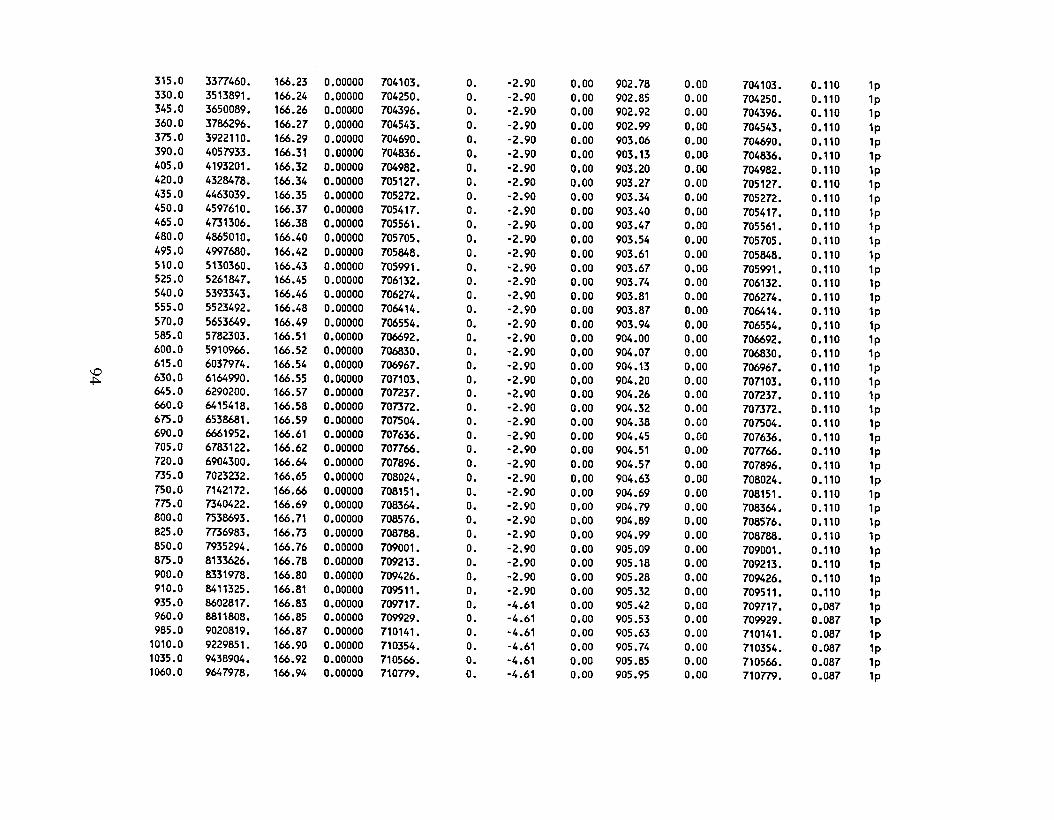
315.0 3377460. 166.23 0.00000 704103. o. -2.90 0.00 902.78 0.00 704103. 0.110 1p330.0 3513891. 166.24 0.00000 704250. o. -2.90 0.00 902.85 0.00 704250. 0.110 1p345.0 3650089. 166.26 0.00000 704396. O. -2.90 0.00 902.92 0.00 704396. 0.110 1p360.0 3786296. 166.27 0.00000 704543. O. -2.90 0.00 902.99 0.00 704543. 0.110 1p375.0 3922110. 166.29 0.00000 704690. O. -2.90 0.00 903.06 0.00 704690. 0.110 1p390.0 4057933. 166.31 0.00000 704836. O. -2.90 0.00 903.13 0.00 704836. 0.110 1p405.0 4193201. 166.32 0.00000 704982. O. -2.90 0.00 903.20 0.00 704982. 0.110 1p420.0 4328478. 166.34 0.00000 705127. O. -2.90 0.00 903.27 0.00 705127. 0.110 1p435.0 4463039. 166.35 0.00000 705272. O. -2.90 0.00 903.34 0.00 7052n. 0.110 1p450.0 4597610. 166.37 0.00000 705417. O. -2.90 0.00 903.40 0.00 705417. 0.110 1p465.0 4731306. 166.38 0.00000 705561. O. -2.90 0.00 903.47 0.00 705561. 0.110 1p480.0 4865010. 166.40 0.00000 705705. O. -2.90 0.00 903.54 0.00 705705. 0.110 1p495.0 4997680. 166.42 0.00000 705848. O. -2.90 0.00 903.61 0.00 705848. 0.110 1p510.0 5130360. 166.43 0.00000 705991. O. -2.90 0.00 903.67 0.00 705991. 0.110 1p525.0 5261847. 166.45 0.00000 706132. O. -2.90 0.00 903.74 0.00 706132. 0.110 1p540.0 5393343. 166.46 0.00000 706274. O. -2.90 0.00 903.81 0.00 706274. 0.110 1p555.0 5523492. 166.48 0.00000 706414. o. -2.90 0.00 903.87 0.00 706414. 0.110 1p570.0 5653649. 166.49 0.00000 706554. O. -2.90 0.00 903.94 0.00 706554. 0.110 1p585.0 5782303. 166.51 0.00000 706692. O. -2.90 0.00 904.00 0.00 706692. 0.110 1p600.0 5910966. 166.52 0.00000 706830. O. -2.90 0.00 904.07 0.00 706830. 0.110 1p615.0 6037974. 166.54 0.00000 706967. O. -2.90 0.00 904.13 0.00 706967. 0.110 1p\D 630.0 6164990. 166.55 0.00000 707103. O. -2.90 0.00 904.20 0.00 707103. 0.110 1p+::-645.0 6290200. 166.57 0.00000 70n37. O. -2.90 0.00 904.26 0.00 70n37. 0.110 1p660.0 6415418. 166.58 0.00000 7073n. o. -2.90 0.00 904.32 0.00 707372. 0.110 1p675.0 6538681. 166.59 0.00000 707504. O. -2.90 0.00 904.38 0.00 707504. 0.110 1p690.0 6661952. 166.61 0.00000 707636. O. -2.90 0.00 904.45 0.00 707636. 0.110 1p705.0 6783122. 166.62 0.00000 707766. O. -2.90 0.00 904.51 0.00 707766. 0.110 1pno.o 6904300. 166.64 0.00000 707896. O. -2.90 0.00 904.57 0.00 707896. 0.110 1p735.0 7023232. 166.65 0.00000 708024. O. -2.90 0.00 904.63 0.00 708024. 0.110 1p750.0 7142172. 166.66 0.00000 708151. O. -2.90 0.00 904.69 0.00 708151. 0.110 1p775.0 7340422. 166.69 0.00000 708364. O. -2.90 0.00 904.79 0.00 708364. 0.110 1p800.0 7538693. 166.71 0.00000 708576. O. -2.90 0.00 904.89 0.00 708576. 0.110 1p825.0 m6983. 166.73 0.00000 708788. O. -2.90 0.00 904.99 0.00 708788. 0.110 1p850.0 7935294. 166.76 0.00000 709001. O. -2.90 0.00 905.09 0.00 709001. 0.110 1p875.0 8133626. 166.78 0.00000 709213. O. -2.90 0.00 905.18 0.00 709213. 0.110 1p900.0 8331978. 166.80 0.00000 709426. O. -2.90 0.00 905.28 0.00 709426. 0.110 1p910.0 8411325. 166.81 0.00000 709511. O. -2.90 0.00 905.32 0.00 709511. 0.110 1p935.0 8602817. 166.83 0.00000 709717. O. -4.61 0.00 905.42 0.00 709717. 0.087 1p960.0 8811808. 166.85 0.00000 709929. O. -4.61 0.00 905.53 0.00 709929. 0.087 1p985.0 9020819. 166.87 0.00000 710141. O. -4.61 0.00 905.63 0.00 710141. 0.087 1p
1010.0 9229851. 166.90 0.00000 710354. O. -4.61 0.00 905.74 0.00 710354. 0.087 1p1035.0 9438904. 166.92 0.00000 710566. O. -4.61 0.00 905.85 0.00 710566. 0.087 1p1060.0 9647978. 166.94 0.00000 710779. O. -4.61 0.00 905.95 0.00 710779. 0.087 1p
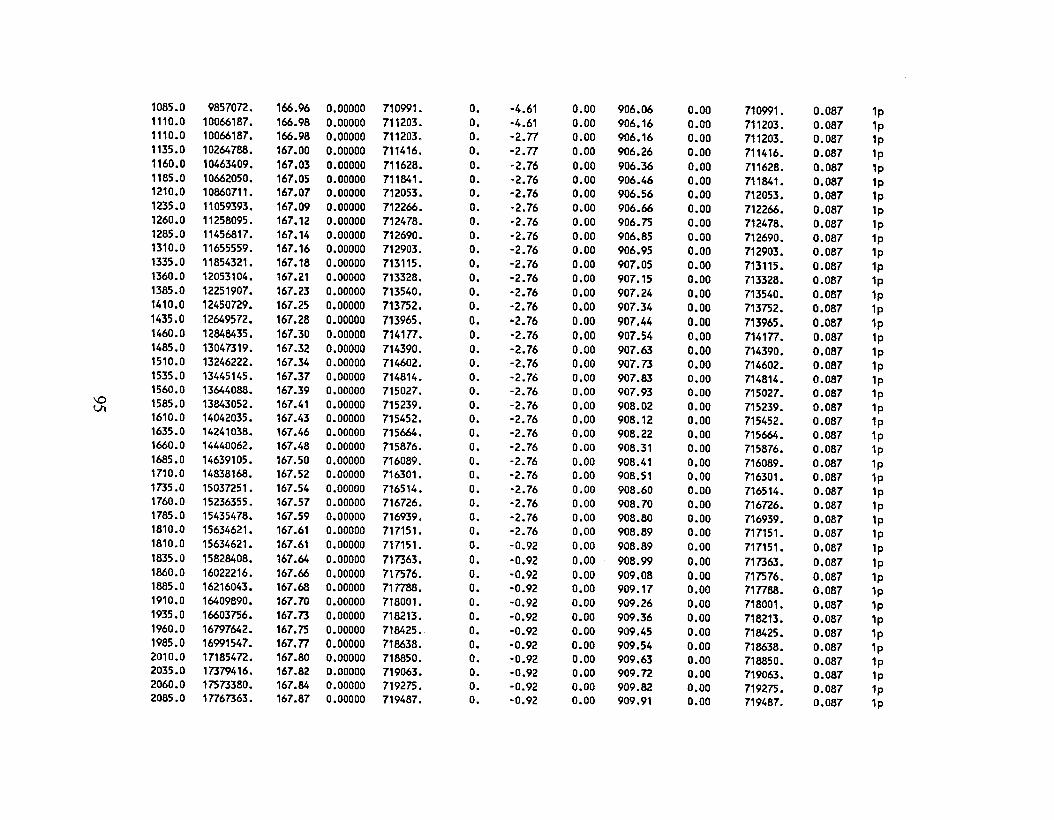
1085.0 9857072. 166.96 0.00000 710991. O. -4.61 0.00 906.06 0.00 710991. 0.087 1p1110.0 10066187. 166.98 0.00000 711203. O. -4.61 0.00 906.16 0.00 711203. 0.087 1p1110.0 10066187. 166.98 0.00000 711203. O. -2.77 0.00 906.16 0.00 711203. 0.087 1p1135.0 10264788. 167.00 0.00000 711416. O. -2.77 0.00 906.26 0.00 711416. 0.087 1p1160.0 10463409. 167.03 0.00000 711628. O. -2.76 0.00 906.36 0.00 711628. 0.087 1p1185.0 10662050. 167.05 0.00000 711841. O. -2.76 0.00 906.46 0.00 711841. 0.087 1p1210.0 10860711. 167.07 0.00000 712053. O. -2.76 0.00 906.56 0.00 712053. 0.087 1p1235.0 11059393. 167.09 0.00000 712266. O. -2.76 0.00 906.66 0.00 712266. 0.087 1p1260.0 11258095. 167.12 0.00000 712478. O. -2.76 0.00 906.75 0.00 712478. 0.087 1p1285.0 11456817. 167.14 0.00000 712690. O. -2.76 0.00 906.85 0.00 712690. 0.087 1p1310.0 11655559. 167.16 0.00000 712903. O. -2.76 0.00 906.95 0.00 712903. 0.087 1p1335.0 11854321. 167.18 0.00000 713115. O. -2.76 0.00 907.05 0.00 713115. 0.087 1p1360.0 12053104. 167.21 0.00000 713328. O. -2.76 0.00 907.15 0.00 713328. 0.087 1p1385.0 12251907. 167.23 0.00000 713540. O. -2.76 0.00 907.24 0.00 713540. 0.087 1p1410.0 12450729. 167.25 0.00000 713752. O. -2.76 0.00 907.34 0.00 713752. 0.087 1p1435.0 12649572. 167.28 0.00000 713965. O. -2.76 0.00 907.44 0.00 713965. 0.087 1p1460.0 12848435. 167.30 0.00000 714177. O. -2.76 0.00 907.54 0.00 714177. 0.087 1p1485.0 13047319. 167.32 0.00000 714390. O. -2.76 0.00 907.63 0.00 714390. 0.087 1p1510.0 13246222. 167.34 0.00000 714602. O. -2.76 0.00 907.73 0.00 714602. 0.087 1p1535.0 13445145. 167.37 0.00000 714814. O. -2.76 0.00 907.83 0.00 714814. 0.087 1p1560.0 13644088. 167.39 0.00000 715027. O. -2.76 0.00 907.93 0.00 715027. 0.087 1p
\0 1585.0 13843052. 167.41 0.00000 715239. O. -2.76 0.00 908.02 0.00 715239. 0.087 1pVI1610.0 14042035. 167.43 0.00000 715452. O. -2.76 0.00 908.12 0.00 715452. 0.087 1p1635.0 14241038. 167.46 0.00000 715664. O. -2.76 0.00 908.22 0.00 715664. 0.087 1p1660.0 14440062. 167.48 0.00000 715876. O. -2.76 0.00 908.31 0.00 715876. 0.087 1p1685.0 14639105. 167.50 0.00000 716089. O. -2.76 0.00 908.41 0.00 716089. 0.087 1p1710.0 14838168. 167.52 0.00000 716301. O. -2.76 0.00 908.51 0.00 716301. 0.087 1p1735.0 15037251. 167.54 0.00000 716514. O. -2.76 0.00 908.60 0.00 716514. 0.087 1p1760.0 15236355. 167.57 0.00000 716726. O. -2.76 0.00 908.70 0.00 716726. 0.087 1p1785.0 15435478. 167.59 0.00000 716939. O. -2.76 0.00 908.80 0.00 716939. 0.087 1p1810.0 15634621. 167.61 0.00000 717151. O. -2.76 0.00 908.89 0.00 717151. 0.087 1p1810.0 15634621. 167.61 0.00000 717151. O. -0.92 0.00 908.89 0.00 717151. 0.087 1p1835.0 15828408. 167.64 0.00000 717363. O. -0.92 0.00 908.99 0.00 717363. 0.087 1p1860.0 16022216. 167.66 0.00000 717576. O. -0.92 0.00 909.08 0.00 717576. 0.087 1p1885.0 16216043. 167.68 0.00000 717788. O. -0.92 0.00 909.17 0.00 717788. 0.087 1p1910.0 16409890. 167.70 0.00000 718001. O. -0.92 0.00 909.26 0.00 718001. 0.087 1p1935.0 16603756. 167.73 0.00000 718213. O. -0.92 0.00 909.36 0.00 718213. 0.087 1p1960.0 16797642. 167.75 0.00000 718425. O. -0.92 0.00 909.45 0.00 718425. 0.087 1p1985.0 16991547. 167.77 0.00000 718638. O. -0.92 0.00 909.54 0.00 718638. 0.087 1p2010.0 17185472. 167.80 0.00000 718850. O. -0.92 0.00 909.63 0.00 718850. 0.087 1p2035.0 17379416. 167.82 0.00000 719063. O. -0.92 0.00 909.72 0.00 719063. 0.087 1p2060.0 17573380. 167.84 0.00000 719275. O. -0.92 0.00 909.82 0.00 719275. 0.087 1p2085.0 17767363. 167.87 0.00000 719487. O. -0.92 0.00 909.91 0.00 719487. 0.087 1p
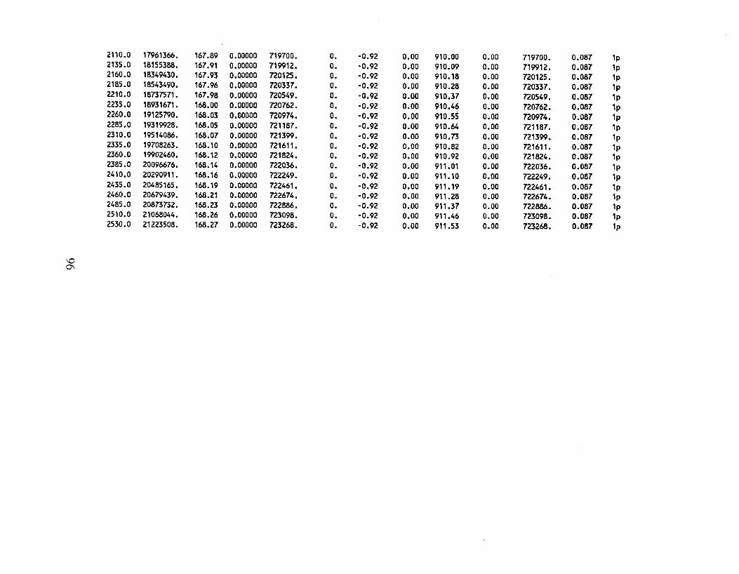
\00\
2110.0 17961366. 167.89 0.00000 719700. O. -0.92 0.00 910.00 0.00 719700. 0.087 1p2135.0 18155388. 167.91 0.00000 719912. O. -0.92 0.00 910.09 0.00 719912. 0.087 1p2160.0 18349430. 167.93 0.00000 n0125. O. -0.92 0.00 910.18 0.00 720125. 0.087 1p2185.0 18543490. 167.96 0.00000 720337. O. -0.92 0.00 910.28 0.00 720337. 0.087 1p2210.0 18737571. 167.98 0.00000 n0549. O. -0.92 0.00 910.37 0.00 n0549. 0.087 1p2235.0 18931671. 168.00 0.00000 n0762. O. -0.92 0.00 910.46 0.00 n0762. 0.087 1p2260.0 19125790. 168.03 0.00000 n0974. O. -0.92 0.00 910.55 0.00 n0974. 0.087 1p2285.0 19319928. 168.05 0.00000 n1187. O. -0.92 0.00 910.64 0.00 n1187. 0.087 1p2310.0 19514086. 168.07 0.00000 721399. O. -0.92 0.00 910.73 0.00 n1399. 0.087 1p2335.0 19708263. 168.10 0.00000 n1611. O. -0.92 0.00 910.82 0.00 n1611. 0.087 1p2360.0 19902460. 168.12 0.00000 721824. O. -0.92 0.00 910.92 0.00 n1824. 0.087 1p2385.0 20096676. 168.14 0.00000 n2036. O. -0.92 0.00 911.01 0.00 n2036. 0.087 1p2410.0 20290911. 168.16 0.00000 722249. O. -0.92 0.00 911.10 0.00 n2249. 0.087 1p2435.0 20485165. 168.19 0.00000 722461. O. -0.92 0.00 911.19 0.00 n2461. 0.087 1p2460.0 20679439. 168.21 0.00000 722674. O. -0.92 0.00 911.28 0.00 n2674. 0.087 1p2485.0 20873732. 168.23 0.00000 722886. O. -0.92 0.00 911.37 0.00 n2886. 0.087 1p2510.0 21068044. 168.26 0.00000 n3098. O. -0.92 0.00 911.46 0.00 723098. 0.087 1p2530.0 21223508. 168.27 0.00000 723268. O. -0.92 0.00 911.53 0.00 723268. 0.087 1p
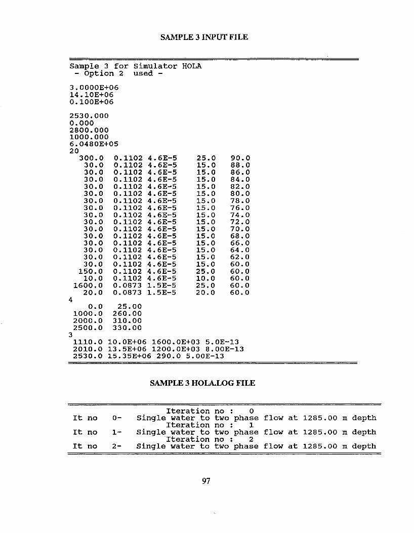
SAMPLE 3 INPUT FILE
Sample 3 for Simulator HOLA- Option 2 used -
3.0000E+0614.10E+060.100E+06
2530.0000.0002800.0001000.0006.0480E+0520
300.0 0.1102 4.6E-5 25.0 90.030.0 0.1102 4.6E-5 15.0 88.030.0 0.1102 4.6E-5 15.0 86.030.0 0.1102 4.6E-5 15.0 84.030.0 0.1102 4.6E-5 15.0 82.030.0 0.1102 4.6E-5 15.0 80.030.0 0.1102 4.6E-5 15.0 78.030.0 0.1102 4.6E-5 15.0 76.030.0 0.1102 4.6E-5 15.0 74.030.0 0.1102 4.6E-5 15.0 72.030.0 0.1102 4.6E-5 15.0 70.030.0 0.1102 4.6E-5 15.0 68.030.0 0.1102 4.6E-5 15.0 66.030.0 0.1102 4.6E-5 15.0 64.030.0 0.1102 4.6E-5 15.0 62.030.0 0.1102 4.6E-5 15.0 60.0
150.0 0.1102 4.6E-5 25.0 60.010.0 0.1102 4.6E-5 10.0 60.0
1600.0 0.0873 1.5E-5 25.0 60.020.0 0.0873 1.5E-5 20.0 60.0
40.0 25.00
1000.0 260.002000.0 310.002500.0 330.00
31110.0 10.0E+06 1600.0E+03 5.0E-132010.0 13.5E+06 1200.0E+03 8.00E-132530.0 15.35E+06 290.0 5.00E-13
SAMPLE 3 HOLA.LOG FILE
Iteration no · 0·It no 0- Single water to two phase flow at 1285.00 m depthIteration no · 1·It no 1- Single water to two phase flow at 1285.00 m depthIteration no · 2·It no 2- Single water to two phase flow at 1285.00 m depth
97
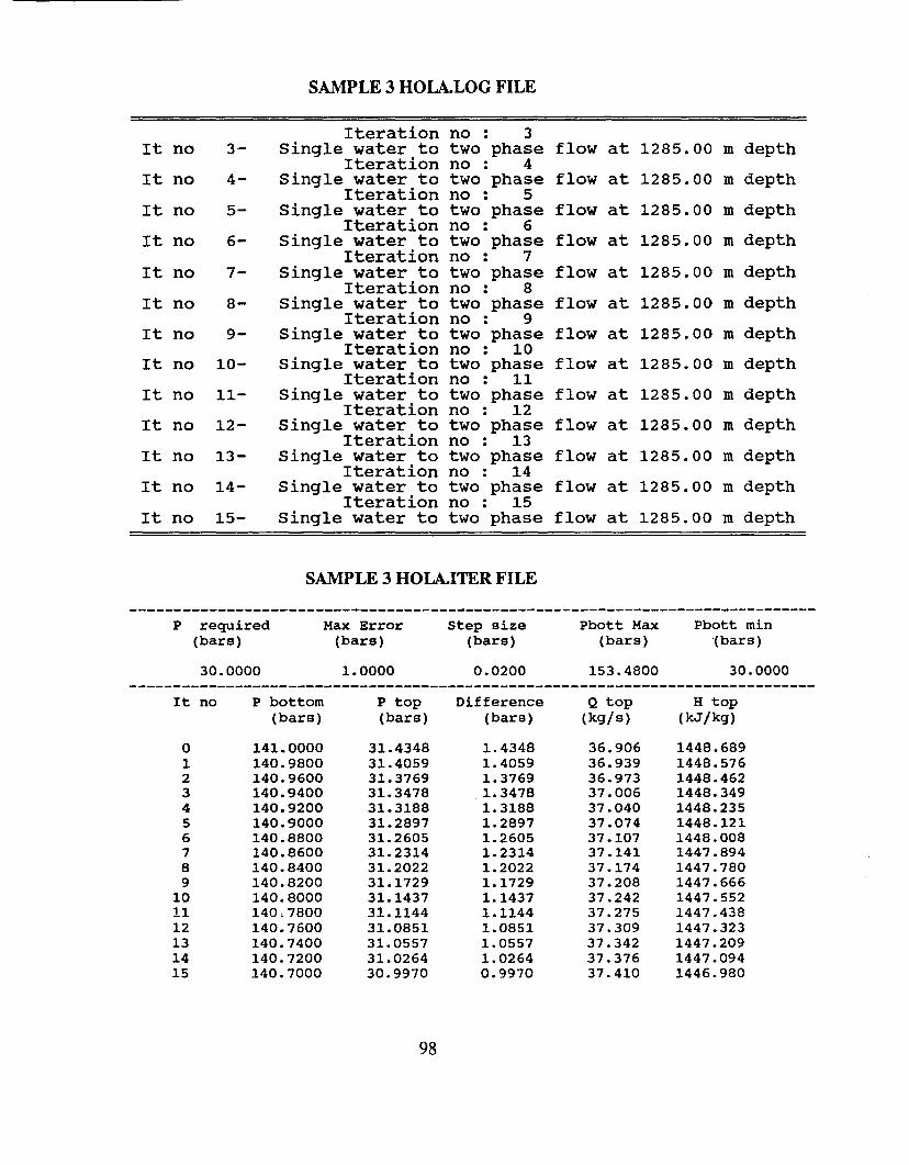
SAMPLE 3 HOLA.LOG FILE
Iteration no · 3·It no 3- Single water to two phase flow at 1285.00 m depthIteration no · 4·It no 4- Single water to two phase flow at 1285.00 m depthIteration no · 5·It no 5- Single water to two phase flow at 1285.00 m depthIteration no · 6·It no 6- single water to two phase flow at 1285.00 m depthIteration no · 7·It no 7- Single water to two phase flow at 1285.00 m depthIteration no · 8·It no 8- Single water to two phase flow at 1285.00 m depthIteration no · 9·It no 9- Single water to two phase flow at 1285.00 m depthIteration no · 10·It no 10- Single water to two phase flow at 1285.00 m depthIteration no · 11·It no 11- Single water to two phase flow at 1285.00 m depthIteration no · 12·It no 12- Single water to two phase flow at 1285.00 m depthIteration no · 13·It no 13- Single water to two phase flow at 1285.00 m depthIteration no · 14·It no 14- Single water to two phase flow at 1285.00 m depthIteration no · 15·It no 15- Single water to two phase flow at 1285.00 m depth
SAMPLE 3 HOLA.ITER FILE
------------------------------------------------------------------------------P required Max Error step size Pbott Max Pbott min
(bars) (bars) (bars) (bars) '(bars)
30.0000 1.0000 0.0200 153.4800 30.0000------------------------------------------------------------------------------
It no P bottom P top Difference Q top H top(bars) (bars) (bars) (k9/s) (kJ/kg)
0 141.0000 31.4348 1.4348 36.906 1448.6891 140.9800 31.4059 1.4059 36.939 1448.5762 140.9600 31.3769 1.3769 36.973 1448.4623 140.9400 31.3478 1. 3478 37.006 1448.3494 140.9200 31.3188 1. 3188 37.040 1448.2355 140.9000 31.2897 1.2897 37.074 1448.1216 140.8800 31.2605 1.2605 37.107 1448.0087 140.8600 31.2314 1.2314 37.141 1447.8948 140.8400 31.2022 1.2022 37.174 1447.7809 140.8200 31.1729 1.1729 37.208 1447.666
10 140.8000 31.1437 1.1437 37.242 1447.55211 140.7800 31.1144 1.1144 37.275 1447.43812 140.7600 31.0851 1.0851 37.309 1447.32313 140.7400 31.0557 1. 0557 37.342 1447.20914 140.7200 31.0264 1.0264 37.376 1447.09415 140.7000 30.9970 0.9970 37.410 1446.980
98
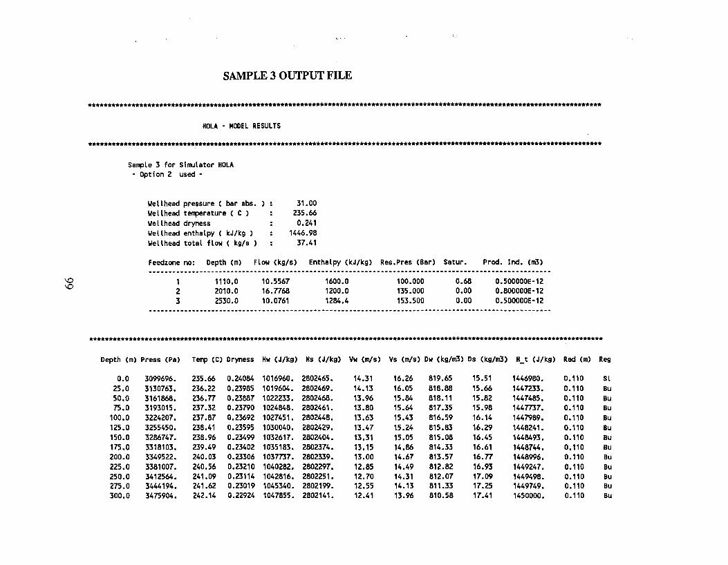
SAMPLE 3 OUTPUT FILE
**********************************************************************************************************************************
HOLA - MODEL RESULTS
**********************************************************************************************************************************
Sample 3 for Simulator HOLA- Option 2 used-
Wellhead pressure ( bar abs.Wellhead temperature ( C )Wellhead drynessWellhead enthalpy ( kJ/kg )Wellhead total flow ( kg/s )
31.00235.660.241
1446.9837.41
Feedzone no: Depth (m) Flow (kg/s) Enthalpy (kJ/kg) Res.Pres (Bar) Satur. Prod. Incl. (m'3)
\0\0
123
1110.02010.02530.0
10.556716.776810.0761
1600.01200.01284.4
100.000135.000153.500
0.680.000.00
0.500000E-120.800000E-120.500000E-12
**********************************************************************************************************************************
Depth (m) Press (Pa) Temp (C) Dryness Hw (J/kg) Hs (J/kg) Vw (m/s) Vs (m/s) Ow (kg/m'3) Os (kg/m'3) H_t (J/kg) Rad (m) Reg
0.0 3099696. 235.66 0.24084 1016960. 2802465. 14.31 16.26 819.65 15.51 1446980. 0.110 Sl25.0 3130763. 236.22 0.23985 1019604. 2802469. 14.13 16.05 818.88 15.66 144n33. 0.110 Bu50.0 3161868. 236.77 0.23887 1022233. 2802468. 13.96 15.84 818.11 15.82 1447485. 0.110 Bu75.0 3193015. 237.32 0.23790 1024848. 2802461. 13.80 15.64 817.35 15.98 144m7. 0.110 Bu
100.0 3224207. 237.87 0.23692 1027451. 2802448. 13.63 15.43 816.59 16.14 1447989. 0.110 Bu125.0 3255450. 238.41 0.23595 1030040. 2802429. 13.47 15.24 815.83 16.29 1448241. 0.110 Bu150.0 3286747. 238.96 0.23499 1032617. 2802404. 13.31 15.05 815.08 16.45 1448493. 0.110 Bu175.0 3318103. 239.49 0.23402 1035183. 2802374. 13.15 14.86 814.33 16.61 1448744. 0.110 Bu200.0 3349522. 240.03 0.23306 1037737. 2802339. 13.00 14.67 813.57 16.77 1448996. 0.110 Bu225.0 3381007. 240.56 0.23210 1040282. 2802297. 12.85 14.49 812.82 16.93 1449247. 0.110 Bu250.0 3412564. 241.09 0.23114 1042816. 2802251. 12.70 14.31 812.07 17.09 1449498. 0.110 Bu275.0 3444194. 241.62 0.23019 1045340. 2802199. 12.55 14.13 811.33 17.25 1449749. 0.110 Bu300.0 3475904. 242.14 0.22924 1047855. 2802141. 12.41 13.96 810.58 17.41 1450000. 0.110 Bu

315.0 3494969. 242.46 0.22866 1049360. 2802104. 12.32 13.86 810.14 17.51 1450150. 0.110 Bu330.0 3514057. 242.77 0.22809 1050862. 2802065. 12.24 13.75 809.69 17.61 1450299. 0.110 Bu345.0 3533177. 243.08 0.22752 1052360. 2802024. 12.15 13.65 809.24 17.70 1450449. 0.110 Bu360.0 3552308. 243.39 0.22695 1053854. 2801981. 12.07 13.55 808.80 17.80 1450598. 0.110 Bu375.0 3571472. 243.70 0.22638 1055345. 2801937. 11.99 13.46 808.35 17.90 1450747. 0.110 Bu390.0 3590633. 244.01 0.22582 1056831. 2801890. 11.91 13.36 807.91 18.00 1450895. 0.110 Bu405.0 3609829. 244.32 0.22525 1058314. 2801842. 11.83 13.26 807.47 18.09 1451044. 0.110 Bu420.0 3629008. 244.63 0.22468 1059791. 2801792. 11.75 13.17 807.03 18.19 1451192. 0.110 Bu435.0 3648223. 244.93 0.22412 1061265. 2801740. 11.67 13.07 806.58 18.29 1451340. 0.110 Bu450.0 3667407. 245.24 0.22356 1062732. 2801686. 11.59 12.98 806.15 18.39 1451487. 0.110 Bu465.0 3686628. 245.54 0.22299 1064197. 2801631. 11.51 12.89 805.71 18.49 1451634. 0.110 Bu480.0 3705804. 245.84 0.22243 1065653. 2801574. 11.43 12.80 805.27 18.58 1451780. 0.110 Bu495.0 3725017. 246.15 0.22187 1067107. 2801515. 11.36 12.71 804.83 18.68 1451926. 0.110 Bu510.0 3744170. 246.45 0.22132 1068552. 2801454. 11.28 12.62 804.40 18.78 1452071. 0.110 Bu525.0 3763361. 246.74 0.22076 1069994. 2801392. 11.21 12.53 803.96 18.88 1452215. 0.110 Bu540.0 3782476. 247.04 0.22020 1071427. 2801329. 11.14 12.44 803.53 18.98 1452359. 0.110 Bu555.0 3801630. 247.34 0.21965 1072857. 2801263. 11.06 12.35 803.10 19.08 1452502. 0.110 Bu570.0 3820691. 247.63 0.21910 1074276. 2801196. 10.99 12.27 802.67 19.17 1452644. 0.110 Bu585.0 3839792. 247.92 0.21855 1075693. 2801128. 10.92 12.19 802.24 19.27 1452786. 0.110 Bu600.0 3858784. 248.21 0.21800 1077097. 2801058. 10.85 12.10 801.82 19.37 1452926. 0.110 Bu615.0 3877815. 248.50 0.21746 1078500. 2800987. 10.78 12.02 801.39 19.47 1453066. 0.110 Bu..... 630.0 3896721. 248.79 0.21691 1079889. 2800915. 10.71 11.94 800.97 19.57 1453204. 0.110 Bu0
0 645.0 3915666. 249.07 0.21637 1081277. 2800841. 10.65 11.86 800.55 19.66 1453342. 0.110 Bu660.0 3934469. 249.36 0.21583 1082650. 2800765. 10.58 11. 78 800.13 19.76 1453478. 0.110 Bu675.0 3953310. 249.64 0.21530 1084022. 2800689. 10.51 11.70 799.71 19.86 1453614. 0.110 Bu690.0 3971991. 249.92 0.21476 1085377. 2800611. 10.45 11.63 799.30 19.95 1453748. 0.110 Bu705.0 3990711. 250.19 0.21423 1086732. 2800532. 10.38 11.55 798.89 20.05 1453882. 0.110 Bu720.0 4009253. 250.47 0.21370 1088069. 2800452. 10.32 11.48 798.48 20.15 1454013. 0.110 Bu735.0 4027833. 250.74 0.21318 1089405. 2800371. 10.26 11.40 798.07 20.24 1454145. 0.110 Bu750.0 4046216. 251.01 0.21266 1090724. 2800289. 10.20 11.33 797.67 20.34 1454274. 0.110 Bum.o 4076939. 251.46 0.21179 1092918. 2800149. 10.09 11.21 797.00 20.50 1454490. 0.110 Bu800.0 410mo. 251.91 0.21092 1095109. 2800005. 9.99 11.09 796.32 20.66 1454706. 0.110 Bu825.0 4138711. 252.36 0.21005 1097298. 2799856. 9.89 10.97 795.65 20.82 1454921. 0.110 Bu850.0 4169765. 252.81 0.20918 1099484. 2799704. 9.80 10.86 794.98 20.98 1455137. 0.110 Bu875.0 4200935. 253.25 0.20831 1101668. 2799547. 9.70 10.74 794.31 21.14 1455353. 0.110 Bu900.0 4232225. 253.70 0.20744 1103849. 2799385. 9.60 10.63 793.63 21.30 1455568. 0.110 Bu910.0 4244774. 253.88 0.20709 1104722. 2799319. 9.56 10.59 793.36 21.37 1455654. 0.110 Bu935.0 4297035. 254.61 0.20552 1108336. 2799039. 15.13 16.55 792.25 21.64 1455801. 0.087 Bu960.0 4338496. 255.19 0.20433 1111183. 2798810. 14.93 16.32 791.36 21.86 1456020. 0.087 Bu985.0 4380009. 255.77 0.20315 1114017. 2798574. 14.73 16.10 790.48 22.08 1456239. 0.087 Bu
1010.0 4473568. 257.05 0.20037 1120342. 2798020. 3.24 27.15 788.51 22.57 1456496. 0.087 Bu1035.0 4641400. 259.30 0.19528 1131482. 2796950. 3.22 25.92 785.02 23.45 1456717. 0.087 Bu1060.0 4811969. 261.53 0.19017 1142547. 2795768. 3.19 24.75 781.52 24.35 1456937. 0.087 Bu1085.0 4985228. 263.73 0.18503 1153541. 2794474. 3.17 23.63 778.01 25.28 1457156. 0.087 Bu

1110.0 5161106. 265.90 0.17985 1164463. 2793069. 3.15 22.55 n4.50 26.22 1457374. 0.087 Bu1110.0 5161106. 265.90 0.03555 1164463. 2793069. 2.32 3.83 n4.50 26.22 1222367. 0.087 Bu1135.0 5294781. 267.51 0.03086 1172613. 2791943. 2.29 3.34 n1.86 26.95 1222580. 0.087 Bu1160.0 5423259. 269.04 0.02637 1180330.' 2790813. 2.25 2.91 769.35 27.64 1222792. 0.087 Bu1185.0 5549470. 270.51 0.02197 1187805. 2789661. 2.15 2.59 766.91 28.33 1223005. 0.087 Bu1210.0 5676192. 271.95 0.01758 1195208. 2788462. 2.05 2.28 764.47 29.03 1223218. 0.087 Bu1235.0 5803616. 273.39 0.01317 1202555. 2787216. 1.93 1.99 762.04 29.73 1223430. 0.087 Bu1260.0 5932366. 274.81 0.00873 1209882. 2785916. 1.80 1.72 759.61 30.45 1223643. 0.087 Bu1285.0 60n794. 276.39 0.00000 1223855. 2784400. 1.49 1.49 754.n 31.26 1223856. 0.087 Bu1310.0 6239615. 2n.56 0.00000 1224067. O. 1.49 0.00 754.93 0.00 1224067. 0.087 1p1335.0 6401469. 2n.61 0.00000 1224280. O. 1.49 0.00 755.09 0.00 1224280. 0.087 1p1360.0 6563356. 2n.67 0.00000 1224492. O. 1.48 0.00 755.24 0.00 1224492. 0.087 1p1385.0 6725275. 2n.73 0.00000 1224704. O. 1.48 0.00 755.40 0.00 1224704. 0.087 1p1410.0 6887228. 2n.78 0.00000 1224916. O. 1.48 0.00 755.56 0.00 1224916. 0.087 1p1435.0 7049213. 2n.84 0.00000 1225128. O. 1.48 0.00 755.71 0.00 1225128. 0.087 1p1460.0 7211232. 2n.89 0.00000 1225341. O. 1.48 0.00 755.87 0.00 1225341. 0.087 1p1485.0 7373283. 2n.95 0.00000 1225553. O. 1.48 0.00 756.02 0.00 1225553. 0.087 1p1510.0 7535366 .. 278.01 0.00000 1225765. O. 1.48 0.00 756.18 0.00 1225765. 0.087 1p1535.0 7697483. 278.06 0.00000 12259n. O. 1.48 0.00 756.33 0.00 12259n. 0.087 1p1560.0 7859631. 278.12 0.00000 1226190. O. 1.48 0.00 756.49 0.00 1226190. 0.087 1p1585.0 8021813. 278.17 0.00000 1226402. O. 1.48 0.00 756.64 0.00 1226402. 0.087 1p
"'""" 1610.0 8184027. 278.23 0.00000 1226614. O. 1.48 0.00 756.79 0.00 1226614. 0.087 1p0"'""" 1635.0 8346273. 278.28 0.00000 1226826. O. 1.48 0.00 756.95 0.00 1226826. 0.087 1p
1660.0 8508551. 278.34 0.00000 1227039. O. 1.48 0.00 757.10 0.00 1227039. 0.087 1p1685.0 8670862. 278.39 0.00000 1227251. O. 1.48 0.00 757.26 0.00 1227251. 0.087 1p1710.0 8833205. 278.45 0.00000 1227463. O. 1.48 0.00 757.41 0.00 1227463. 0.087 1p1735.0 8995581. 278.51 0.00000 1227675. O. 1.48 0.00 757.56 0.00 1227675. 0.087 1p1760.0 9157989. 278.56 0.00000 1227887. O. 1.48 0.00 757.71 0.00 1227887. 0.087 1p1785.0 9320428. 278.62 0.00000 1228100. O. 1.48 0.00 757.87 0.00 1228100. 0.087 1p1810.0 9482900. 278.67 0.00000 1228312. O. 1.48 0.00 758.02 0.00 1228312. 0.087 1p1835.0 9645404. 278.73 0.00000 1228524. O. 1.48 0.00 758.17 0.00 1228524. 0.087 1p1860.0 9807940. 278.78 0.00000 1228736. O. 1.48 0.00 758.32 0.00 1228736. 0.087 1p1885.0 9970508. 278.84 0.00000 1228949. O. 1.48 0.00 758.47 0.00 1228949. 0.087 1p1910.0 10133107. 278.89 0.00000 1229161. O. 1.48 0.00 758.63 0.00 1229161. 0.087 1p1935.0 10295739. 278.95 0.00000 1229373. O. 1.48 0.00 758.78 0.00 1229373. 0.087 1p1960.0 10458402. 279.00 0.00000 1229585. O. 1.48 0.00 758.93 0.00 1229585. 0.087 1p1985.0 10621098. 279.06 0.00000 1229798. O. 1.48 0.00 759.08 0.00 1229798. 0.087 1p2010.0 10783824. 279.11 0.00000 1230010. O. 1.48 0.00 759.23 0.00 1230010. 0.087 1p2010.0 10783824. 288.62 0.00000 1279976. O. 0.57 0.00 741.12 0.00 1279976. 0.087 1p2035.0 10941481. 288.68 0.00000 1280189. O. 0.57 0.00 741.28 0.00 1280189. 0.087 1p2060.0 11099172. 288.74 0.00000 1280401. O. 0.57 0.00 741.44 0.00 1280401. 0.087 1p2085.0 11256896. 288.80 0.00000 1280613. O. 0.57 0.00 741.60 0.00 1280613. 0.087 1p2110.0 11414654. 288.86 0.00000 1280825. O. 0.57 0.00 741.75 0.00 1280825. 0.087 1p2135.0 11572446. 288.92 0.00000 1281037. O. 0.57 0.00 741.91 0.00 1281037. 0.087 1p
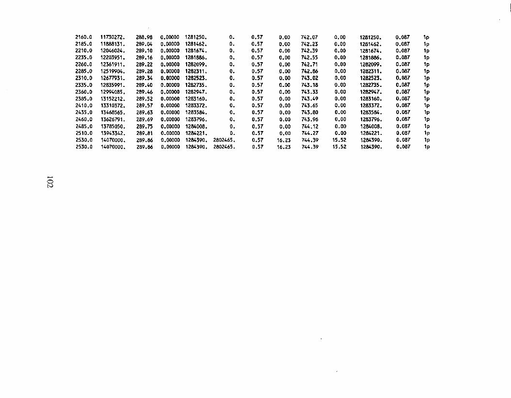
......otv
2160.0 11730272. 288.98 0.00000 1281250. o. 0.57 0.00 742.07 0.00 1281250. 0.087 1p2185.0 11888131. 289.04 0.00000 1281462. o. 0.57 0.00 742.23 0.00 1281462. 0.087 1p2210.0 12046024. 289.10 0.00000 1281674. o. 0.57 0.00 742.39 0.00 1281674. 0.087 1p2235.0 12203951. 289.16 0.00000 1281886. o. 0.57 0.00 742.55 0.00 1281886. 0.087 1p2260.0 12361911. 289.22 0.00000 1282099. o. 0.57 0.00 742.71 0.00 1282099. 0.087 1p2285.0 12519904. 289.28 0.00000 1282311. o. 0.57 0.00 742.86 0.00 1282311. 0.087 1p2310.0 12677931- 289.34 0.00000 1282523. o. 0.57 0.00 743.02 0.00 1282523. 0.087 1p2335.0 12835991. 289.40 0.00000 1282735. o. 0.57 0.00 743.18 0.00 1282735. 0.087 1p2360.0 12994085. 289.46 0.00000 1282947. o. 0.57 0.00 743.33 0.00 1282947. 0.087 1p2385.0 13152212. 289.52 0.00000 1283160. o. 0.57 0.00 743.49 0.00 1283160. 0.087 1p2410.0 13310372. 289.57 0.00000 1283372. o. 0.57 0.00 743.65 0.00 1283372. 0.087 1p2435.0 13468565. 289.63 0.00000 1283584. o. 0.57 0.00 743.80 0.00 1283584. 0.087 1p2460.0 13626791- 289.69 0.00000 1283796. o. 0.57 0.00 743.96 0.00 1283796. 0.087 1p2485.0 13785050. 289.75 0.00000 1284008. o. 0.57 0.00 744.12 0.00 1284008. 0.087 1p2510.0 13943342. 289.81 0.00000 1284221. o. 0.57 0.00 744.27 0.00 1284221. 0.087 1p2530.0 14070000. 289.86 0.00000 1284390. 2802465. 0.57 16.23 744.39 15.52 1284390. 0.087 1p2530.0 14070000. 289.86 0.00000 1284390. 2802465. 0.57 16.23 744.39 15.52 1284390. 0.087 1p
Related Documents