Lawrence Berkeley Laboratory - eScholarship

LBL-9741 ~I ~

Lawrence Berkeley LaboratoryUNIVERSITY OF CALIFORNIA

Accelerator & FusionResearch Division

Presented at the 1979 Isabelle Workshop, Upton, NY,July 16-27, 1979

A STUDY OF MICROWAVE INSTABILITIES BY MEANS OFA SQUARE-WELL POTENTIAL

(I

Kwang-Je Kim

September 1979

TWO-WEEK LOAN COpy

- This is a Library Circulating Copywhich may be borrowed for two weeks.For a personal retention copy, callTech. Info. Dioision, Ext. 6782

RECEIVEDlAWRENCE

BERKIilEY LABORATORY

OCT 171979

LIBRARY ANDDOCUMENTS SECTION

Prepared for the U.S. Department of Energy under Contract W-7405-ENG-48

•

Lawrence Berkeley laboratory LibraryUniversity of California, Berkeley

-','

A Study of Microwave Instabilities by means of a

Square-Well Potential

Kwang-Je Kim

Lawrence Berkeley Laboratory

1 Cyclotron Road

Berkeley, CA 94720

(To be published in the proceedings of 1979 ISABELLE workshop on

Beam Current Limitations in Storage Rings.)

I. Introduction

The subject of microwave instabilities has attracted a lot of

theoretical activity recently. A series of papers by Sacherer 1

has played the leading role in the field. Further development of

his work is being actively pursued by several authors 2• However,

the mathematical complexity of the theory makes it very hard to

grasp the essential physics underlying microwave instabilities.

This is rather unfortunate since the qualitative features of

microwave instabilities are easy to understand 3 by applying

coasting beam theory4.

In this paper, microwave instabilities are analyzed in a

simple model, in which the usual synchrotron oscillation of a

particle is replaced by particle motion in a square-well potential.

The motivation for doing this was the following: In the usual

synchrotron oscillation, a particle moves along an elliptic

trajectory. The most natural coordinates for such a motion are the

action and the angle variables. On the other hand, the distribution

of the particles along the ring is most conveniently described by

azimuthal variables. The complexity of the theory of microwave

instabilities derives from the fact that the two sets of the

variables are not simply related. The difficulty disappears if the

~ynchrotron motion is approximated by the motion in a square-well

potential.

The square-well potential may seem extremely unphysical.

However, it should be remarked that the form of the potential with u

addition of a Landau cavity looks more or less like a square-well.

At any rate, the main motivation of introducing the square-well here

is to simplify the mathematics of and thereby gaining some insight

into microwave instabilities.

2

(1)

"

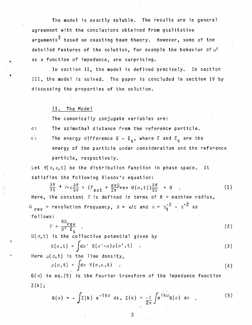
The model is exactly soluble. The results are in general

agreement with the conclusions obtained from qualitative

arguments 3 based on coasting beam theory. However, some of the

detailed features of the solution, for example the behavior ofw2

as a function of impedance, are surprising.

In section II, the model is defined precisely. In section

III, the model is solved. The paper is concluded in section IV by

discussing the properties of the solution.

II. The Model

The canonically conjugate variables are:

a: The azimuthal distance from the reference particle.

€: The energy difference E - Es ' where E and Es are the

energy of the particle under consideration and the reference

particle, respectively.

Let 1£'( a, €, t) be the distribution function in phase space. It

satisfies the following Vlasovls equation:

al£' + aI£' (evQ aI£'at ~'€aa + Fext + ~rev U(a,t))as = 0

Here, the constant f i s defined in terms of R =m achi ne radius,

Q rev = revolution frequency, (3 = vIc and n = Yt 2 - y-2 as

follows:

f' = RQ rev (2)'(32 E

sU(a,t) is the collective potential given by

U(a,t) = fda l G(al-a)p(al,t) (3)

Herep( a, t ) i s the 1i ned ens ity ,

p ( a , t) .= Jd € I£' ( a , € , t ) ( 4 )

G(a) in eq.(5) is the Fourier transform of the impedance function

Z(k) ;

G(a) = - ~Z(k) e- ika dk, Z(k)

3

( 5 )

( 6 )

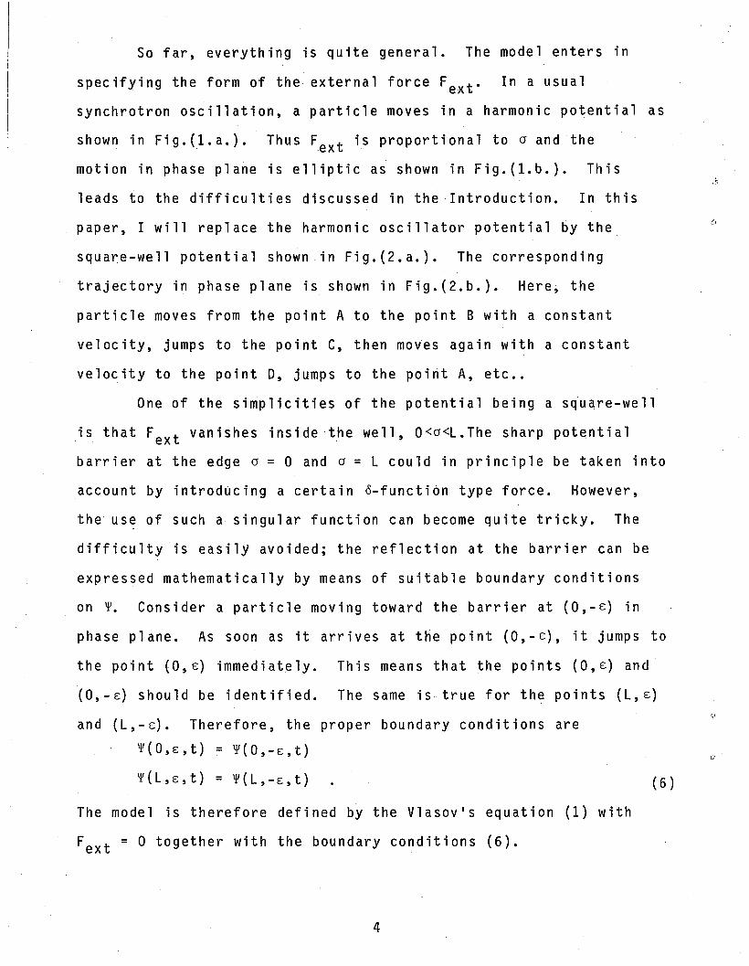
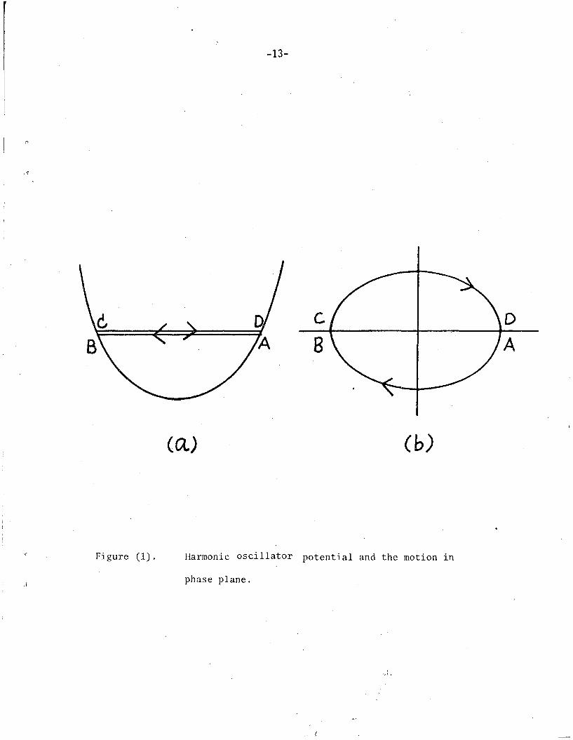
So far, everything is quite general. The model enters in

specifying the form of the external force Fext • In a usual

synchrotron oscillation, a particle moves in a harmonic potential as

shown in Fig.(l.a.). Thus Fext is proportional to a and the

motion in phase plane is elliptic as shown in Fig.(l.b.). This

leads to the difficulties discussed in the -Introduction. In this

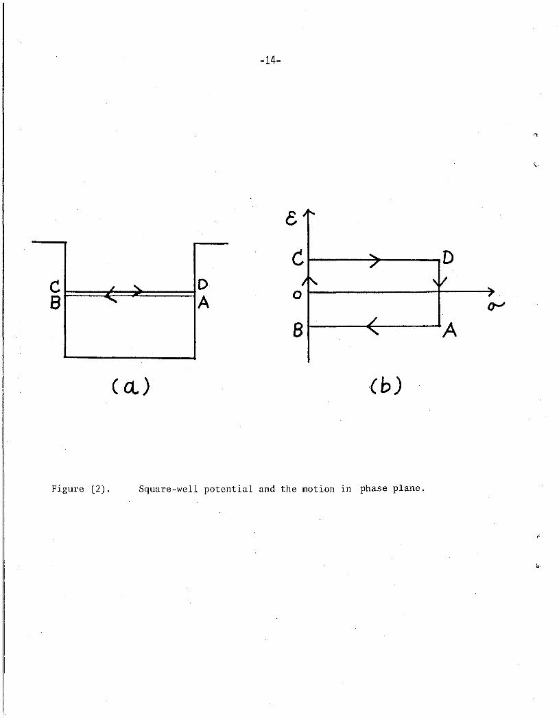
paper, I will replace the harmonic oscillator potential by the

square-well potential shown in Fig.(2.a.). The corresponding

trajectory in phase plane is shown in Fig.(2.b.). Here, the

particle moves from the point A to the point B with a constant

velocity, jumps to the point C, then moves again with a constant

velocity to the point D, jumps to the point A, etc ••

One of the simplicities of the potential being a square-well

is that Fext vanishes inside the well, O<a<L.The sharp potential

barrier at the edge a = 0 and a = L could in principle be taken into

account by introducing a certain a-function type force. However,

the use of such a singular function can become quite tricky. The

difficulty is easily avoided; the reflection at the barrier can be

expressed mathematically by means of suitable boundary conditions

on~. Consider a particle moving toward the barrier at (O,-E) in

phase plane. As soon as it arrives at the point (O,-E), it jumps to

the point (O,E) immediately. This means that the points (O,E) and

(O,-E) should be identified. The same is true for the points (L,E)

and (L,-E). Therefore, the proper boundary conditions are

~(O,E,t) = ~(O,-E,t)

~(L,E,t) = ~(L,-E,t)

The model is therefore defined by the Vlasov's equation (1) with

Fext = 0 together with the boundary conditions (6).

4

( 8 )

( 9 )

..

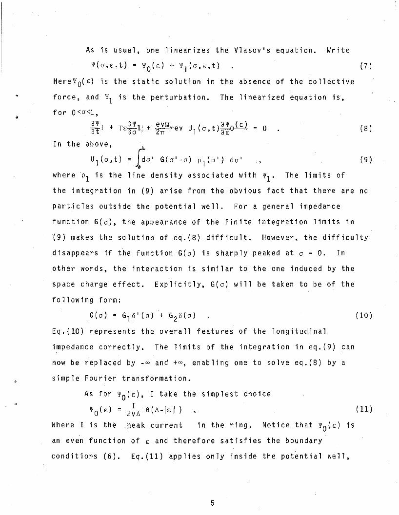
As is usual~ one linearizes the Vlasov's equation. Write

'¥(a,E:t) = '¥O(E) + '¥l(a,E,t) (7)

Here'¥O(E) is the static solution in the absence of the collective

force~ and '1'1 is the perturbation. The linearized equation is,

for o<a<L~

~1 + rE~1,\ + evSG rev U1 (a , t ) ~ ~01£L 0at dO r; ""21f Oc.. =

In the above~L

Ul (a,t) = Ida' G(a' -a) p (a') dal .,o 1

where PI is the line density associated with '1'1. The limits of

the integration in (9) arise from the obvious fact that there are no

particles outside the potential well. For a general impedance

function G(a)~ the appearance of the finite integration limits in

(9) makes the solution of eq.(8) difficult. However~ the difficulty

disappears if the function G(a) is sharply peaked at a = O. In

other words~ the interaction is similar to the one induced by the

space charge effect. Explicitly~ G(a) will be taken to be of the

following form:

G( a) = G10 I (a)+ G20 ( a )

Eq.(10) represents the overall features of the longitudinal

impedance correctly. The limits of the integration in eq.(9) can

now be replaced by _00 and +oo~ enabling one to solve eq.(8) by a

simple Fourier transformation.

As for '¥O(E)~ I take the simplest choice

'¥O(E) = 2~6 e(6-/E/)

(10 )

( 11 )

Where I is the peak current in the ring. Notice that '¥O(E) is

an even function of E and therefore satisfies the boundary

conditions (6). Eq.(ll) applies only inside the potential well~

5

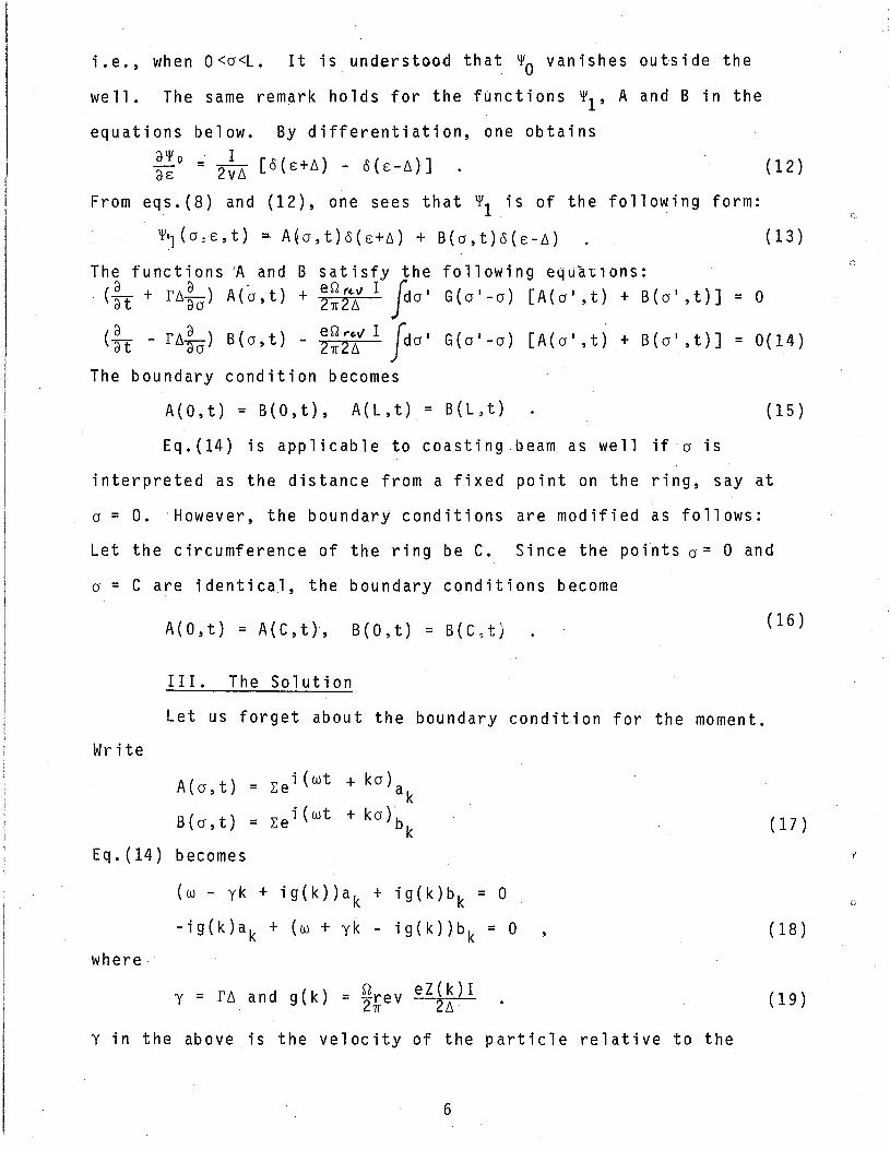
i.e., when O<a<L. It is understood that '¥o vanishes outside the

well. The same rem~rk holds for the functions '¥1' A and B in the

equations below. By differentiation, one obtainsd'¥o . IdE = 2v~ [O(E+~) - O(E-~)] (12)

From eqs.(8) and (12), one sees that '¥1 is of the following form:

'¥Il (a: E, t) =- A~ a , t) 0 ( E+~) + B(a , t ) 0 ( E- ~ ) ( 13 )

The functions 'A and B satisfy the following equations:(~t + r~~a) A(a,t) + 2~27 I pal G(al-a) [A(a',t) + B(a' ,t)] = 0

( ~ t - r ~ ~ a ) B(a , t) - 2~ £[;' I Jd a I G( a I - a ) [ A( a I , t) + B(a I ,t)] = 0( 14)

The boundary condition becomes

A(O,t) = B(O,t), A(L,t) = B(L,t) (15)

Eq.(14) is applicable to coasting.beam as well if'a is

interpreted as the distance from a fixed point on the ring, say at

a = O.However, the boundary conditions are modified as follows:

Let the circumference of the ring be C. Since the points a= 0 and

a = C are identical, the boundary conditions become

A(O,t) = A(C,t), B(O,t) = B(C.t)

III. The Solution

(16 )

Let us forget about the boundary condition for the moment.

( 17)

(w - yk + ig(k))a k + ig(k)b k = °-ig(k)a k + (w + yk - ig(k))b k = 0

where

y in the above is the velocity of the particle relative to the

6

(18)

(19 )

[)

..

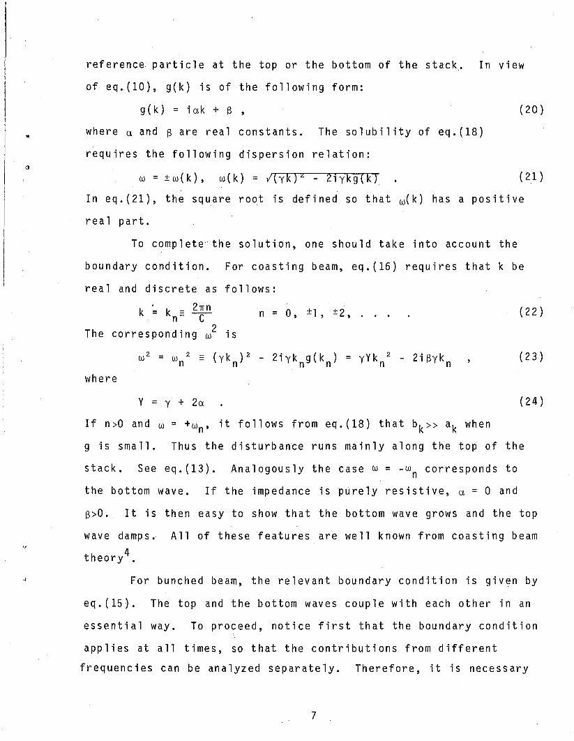
reference particle at the top or the bottom of the stack. In view

of eq.(lO), g(k) is of the following form:

g(k) = iak + S , (20)

where a and S are real constants. The solubility of eq.(18)

requires the following dispersion relation:

w = ±w(k), w(k) = l{yk)Z - 2iykg(k) (21)

In eq.(21), the square root is defined so that w(k) has a positive

rea 1 part.

To completeGthe solution, one should take into account the

boundary condition. For coasting beam, eq.(16) requires that k be

real and discrete as follows:

n = 0, ±l, ±2, ...k ~ kn:: 2~n

The corresponding w2 is

w2 = wn2

:: (Yk n)2 - 2iyk ng(k n) = yYk n2

- 2iSyk nwhere

(22)

(23)

Y = y + 2a (24 )

If n>O and w = +wn, it follows from eq.(18) that bk» ak when

g is small. Thus the disturbance runs mainly along the top of the

stack. See eq.(13). Analogously the case w = -wn corresponds to

the bottom wave. If the impedance is purely resistive, a = 0 and

s>O. It is then easy to show that the bottom wave grows and the top

wave damps. All of these features are well known from coasting beam

theory4.

For bunched beam, the relevant boundary condition is given by

eq.(15). The top and the bottom waves couple with each other in an

essential way. To proceed, notice first that the boundary condition

applies at all times, so that the contributions from different

frequencies can be analyzed separately. Therefore, it is necessary

7

to find the k's which correspond to the same

equation

w2 = (yk)2 - 2iykg(k)

2w • Consider the

(25)

which is equivalent to eq.(21). From eqs.(20) and (25), one obtains

k = k = l@.+ I~ _(~)2 (26)± Y - Yy Y ,

where Y is defined in eq.(24). The functions A and B that behave as

are, in view of eqs.(17)A(o,t) = e iwt (e ik+o

B(o,t) = eiwt(e ik+o

where

and (l8), as follows:

+ i k ° )a+ e - a

b+ + e i k ° b ) (27)

b± = D±a± ' Dj:

The boundary condition

(28)

(30)

( 1 - D+) a+ + ( 1 - D ) a. = 0 (29.a)-( 1 - D+)e i k.j. L

a+ + ( 1 D )e i k L0 (29.b)- - a =

One way to satisfy eq.(29) is to require

D± = 1 and a.~ = 0

After some algebra, one finds that eqs. (25) and (30) imply

w = 0, k = iK = 2if (31)

For this value of wand k, A is identical to B and given by

A(o,t) = B(o,t) = eKO (32)

This solution is time independent and therefore stable.

Eq.(29) can also be satisfied if the two amplitudes a+ and

a are related by (29.a) and, furthermore, k+ and k are

related as follows:

k+ - k = 2K- n2nn= -L- n = 0,1,2, ... (33)

From (26), one obtainsw2 = w 2 = y(YK 2 + ~2)

n n Y

8

(34)

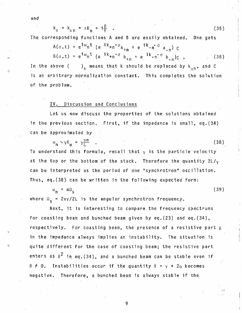
and

k± = k . = ±K + . 13 (35)1-±n n Y

The corresponding functions A and B are ea s il y obtained. One gets

A(o,t) = eiwn t (e ik+n·o + e i k . ° a_ n)a+ n -n C

B(o,t) = eiwn t (e ik '0b+ n + i k .° b )C (36)t) +n e -n -n

In the above ( )± means that k should be replaced by kin' and C,]

is an arbitrary normalization constant. This completes the solution

of th e problem.

IV. Discussion and Conclusions

Let us now discuss the properties of the solutions obtained

in the previous section. First, if the impedance is small, eq.(34)

can be approximated by

w rvyK = ynn (38)n n L

To understand this formula, recall that y is the particle velocity

at the top or the bottom of the stack. Therefore the quantity 2L/y

can be interpreted as the period of one "synchrotron" oscillation.

Thus, eq.(38) can be written in the following expected form:

w = nDn s

where D = 2ny/2L is the angular synchrotron frequency.s

Next, it is interesting to compare the frequency spectrums

for coasting beam and bunched beam given by eq.(23) and eq.(34),

(39)

respectively. For coasting beam, the presence of a resistive part B

in the impedance always implies an instability. The situation is

quite different for the case of coasting beam; the resistive part

enters as 13 2 i~ eq.(34), and a bunched beam can be stable even if

13 f O. Instabilities occur if the quantity Y = y + 2a becomes

negative. Therefore, a bunched beam is always stable if the

9

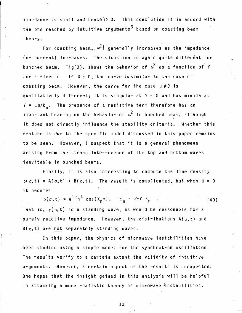
impedance is small and henceY> O. This conclusion is in accord with

the on~ reached by intuitive arguments 3 based on coasting beam

theory.

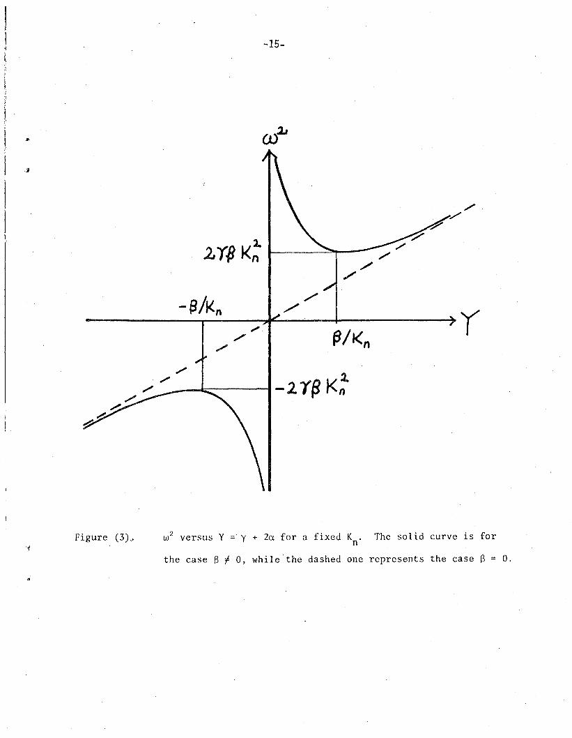
For coasting beam, I w2 / generally increases as the impedance

(or current) increases. The situation is again quite differ~nt for

bunched beam. Fig(3). shows the behavior of w2 as a function of Y

for a fixed n. If [3::: 0, the curve is similar to the case of

coasting beam. However, the curve for the case [3 ~ 0 is

qualitatively different; It is singular at Y = 0 and has minima at

Y = ±[3/k n. The presence of a resistive term therefore has an

important bearing on the behavior of w2 in bunched beam, although

it does not directly influence the stability criteria. Whether this

feature is due to the specific model discussed in this paper remains

to be seen. However, I suspect that it fs a general phenomena

arising from the strong interference of the top and bottom waves

inevitable in bunched beams.

Finally, it is also interesting to compute the line density

p(a,t) = A(a,t) + B(a,t). The result is complicated, but when [3 = 0

it becomes

p(a,t) = .eiwn t cos(Kna), (40)

arguments. However, a certain aspect of the results is unexpected.

One hopes that the insight gained in this analysis will be helpful

in attacking a more realistic theory of microwave·~nstabi1ities.

10 .

. 1

Acknowledgement: I thank the participants of the workshop for

stimulating discussions, especially Dr. E. Courant, Dr. C.

Pellegrini, Dr. A.G. Ruggiero and Dr. M. Sands. I am grateful to

Dr. L. Smith and Dr. A.M. Sessler for useful remarks and for

critically reading this manuscript •

v. Addded Notes

If the resistive part S is due to the skin effect, it is of

the form

S = (1 + i)Bo

where 130 is a real .constant. From this and eq.(23), one sees

that 13 0 is the growth rate for coasting beam in the case of y»a.

The growth rate for bunched beam is found by inserting the above

formula into eq.(34), and one finds

In other words, the growth rate for bunched beam is reduced by a

factor Bo/ns compared to the growth rate of coasting beam, 130.

Dr. L. Smith has obtained the dispersion relation (34) by

; using the technique of integrating over unperturbed orbit. The same

technique can be used to justify the boundary condition (6) on a

more rigorous basis.

',!.,

11

References:

1) Sacherer, F., IEEE Trans., Vol. NS-24, No.3, 1393 (1977) and

references cited therein.

2 ) Besnier, G., Contribution a L'etude des Petites Oscillations

Longitudinales d'un Faisceau, Univ. of Rennes Report."

Laclare, J.L., Lab. National Saturne Report (1977).

Pellegrini, C. and J.M. Wang, to be published.

3) Hereward, H., Proc. 1975 ISABELLE Summer Study, Brookhaven,

BNL 20550, P. 555.

4) Neil, V.K., and A.M. Sessler, Rev. Sci. Instr. ~, 429 (1965).

,',1',

12

-13-

(ct)

c8

(b)

D

A

Figure (1). Harmonic oscillator potential and the motion in

phase plane.

,'./ ..

-14-

J----~---D

B A

(b)

Figure (2). Square-well potential and the motion in phase plane.

-15-

2Y$K~

,,-/-~---I-2 r~ K;

Figure (3) " w2 versus y = y + 2a for a fixed K The solid curve is for'r

n

the case f3 t a, while the dashed one represents the case f3 = a.

"

This report was done with support from theDepartment of Energy. Any conclusions or opinionsexpressed in this report represent solely those of theauthor(s) and not necessarily those of The Regents ofthe University of California. the Lawrence BerkeleyLaboratory or the Department of Energy.

Reference to a company or product name doesnot imply approval or recommendation of theproduct by the University of California or the U.S.Department of Energy to the exclusion of others thatmay be suitable.

TECHNICAL INFORMATION DEPARTMENT

LAWRENCE BERKELEY LABORATORY

UNIVERSITY OF CALIFORNIA

BERKELEY, CALIFORNIA 94720