Latent Space Energy-Based Model - eScholarship

UNIVERSITY OF CALIFORNIA

Los Angeles

Latent Space Energy-Based Model

A dissertation submitted in partial satisfaction

of the requirements for the degree

Doctor of Philosophy in Statistics

by

Bo Pang

2021

© Copyright by

Bo Pang

2021

ABSTRACT OF THE DISSERTATION

Latent Space Energy-Based Model

by

Bo Pang

Doctor of Philosophy in Statistics

University of California, Los Angeles, 2021

Professor Yingnian Wu, Chair

In this dissertation, we seek a simple and unified probabilistic model, with power endowed with

modern neural networks and computing hardware, that is versatile to model patterns of high

dimensionality and complexity in various domains such natural images and natural language. We

achieve the goal by studying three families of probabilistic models and proposing a unification of

them, which leads to a simple but rather versatile model with rich applications in various domains.

In the modern deep learning era, three families of probabilistic models are widely used to model

complex patterns. One family is generator model, which assumes that the observed example is

generated by a low-dimensional latent vector via a top-down network and the latent vector follows

a non-informative prior distribution. The second family is energy-based model (EBM), which

specifies a probability distribution of the observed example, based on an energy function defined

on the observed example and parameterized by a bottom-up deep network. The third family is

discriminative model which is in the form of classifiers and specifies the conditional probability of

the output class label given an input signal.

EBM is expressive but poses challenges in sampling since the energy function defined in the data

space has to be highly multi-modal in order to fit the usually multi-modal data distribution, while

ii

generator model is relatively less expressive but convenient and efficient in terms of sampling owing

to its simple factorized form. We first integrate these two models. In particular, we propose to learn

an EBM in the latent space as the prior distribution of the generator model, following the philosophy

of empirical Bayes. We call the proposed model as latent space energy-based model, consisting of

the energy-based prior model and the top-down generation model. Due to the low dimensionality

of the latent space, a simple energy function in latent space can capture regularities in the data

effectively. Thus, the resulting model is much more expressive than the original generator model

with little cost in terms of model complexity and computational complexity. Also, MCMC sampling

in the latent space is much more efficient and mixes better than that in the observed data space.

Furthermore, we introduce a principled learning algorithm which is formulated as a perturbation of

maximum likelihood learning in terms of both objective function and estimating equation, so that

the learning algorithm has a solid theoretical foundation.

We verify the proposed model and learning algorithm on a variety of image and text datasets such

as human faces, financial news. The model is able to effectively learn from these high-dimensional

and complex datasets. As a result, we can sample faithful and diverse samples from the learned

models. We also find that since the model is well-learned, it leads to a discriminative latent space

that separates probability densities for normal and anomalous data, naturally making this model a

tool for anomaly detection.

Having established the effectiveness of the proposed latent space EBM and learning algorithm,

we explore two applications which leverage two respective aspects of latent space EBM. In one

application, we exploit the expressiveness of latent space EBM and use it to model molecules which

are encoded in a simple format of linear strings. Despite its convenience, models relying on this

simple representation tend to generate invalid samples and duplicates. Due to its expressiveness,

learned latent space EBM on molecules in this simple and convenient representation is able to

generate molecules with validity, diversity and uniqueness competitive with state-of-the-art models,

and generated molecules have structural and chemical features whose distributions almost perfectly

match those of the real molecules. In another application, we explore the aspect of EBM as a cost

iii

function and make a connection with inverse reinforcement learning for diverse human trajectory

forecasting. The cost function is learned from expert demonstrations projected into the latent space.

To make a forecast, optimizing the cost function leads to a belief vector, which is then projected to

the trajectory space by a policy network. The proposed model can make accurate, multi-modal, and

social compliant trajectory predictions.

Building on top of the unification of generator model and EBM, we further integrates discrimi-

native model into latent space EBM via an energy term that couples a continuous latent vector and

a symbolic one-hot vector. With such a coupling formulation, discrete category can be inferred

from the observed example based on the continuous latent vector. Also, the latent space coupling

naturally enables incorporation of information bottleneck regularization to encourage the continuous

latent vector to extract information from the observed example that is informative of the underlying

category. In our learning method, the symbol-vector coupling, the generator network and the

inference network are learned jointly. Our model can be learned in either an unsupervised setting

or a semi-supervised setting where category labels are provided for a subset of training examples.

With the symbol-vector coupling, the learned latent space is well-structured such that the generator

generates text with high-quality and interpretability and it performs well on classification tasks with

a limited amount of labeled data.

iv

The dissertation of Bo Pang is approved.

Qing Zhou

Hongquan Xu

Mark Stephen Handcock

Yingnian Wu, Committee Chair

University of California, Los Angeles

2021

v

To my parents and my wife

for their support and love

vi

TABLE OF CONTENTS

1 Introduction . . . . . . . . . . . . . . . . . . . . . . . . . . . . . . . . . . . . . . . 1

1.1 Unifying Three Families of Probabilistic Models . . . . . . . . . . . . . . . . . . 2

1.1.1 Langevin Dynamics . . . . . . . . . . . . . . . . . . . . . . . . . . . . . 2

1.1.2 Energy-Based Model . . . . . . . . . . . . . . . . . . . . . . . . . . . . . 3

1.1.3 Generator Model . . . . . . . . . . . . . . . . . . . . . . . . . . . . . . . 4

1.1.4 Terminology Clarification . . . . . . . . . . . . . . . . . . . . . . . . . . 5

1.1.5 Unification of Generator Model and Energy-Based Model . . . . . . . . . 6

1.1.6 Discriminative Model . . . . . . . . . . . . . . . . . . . . . . . . . . . . 6

1.1.7 Unification of Latent Space Energy-Based Model and Discriminative Model 7

1.2 Overview of the Dissertation . . . . . . . . . . . . . . . . . . . . . . . . . . . . . 8

2 Latent Space Energy-Based Model . . . . . . . . . . . . . . . . . . . . . . . . . . 11

2.1 Introduction . . . . . . . . . . . . . . . . . . . . . . . . . . . . . . . . . . . . . . 11

2.2 Model and learning . . . . . . . . . . . . . . . . . . . . . . . . . . . . . . . . . . 13

2.2.1 Model . . . . . . . . . . . . . . . . . . . . . . . . . . . . . . . . . . . . . 13

2.2.2 Maximum likelihood . . . . . . . . . . . . . . . . . . . . . . . . . . . . . 14

2.2.3 Short-run MCMC . . . . . . . . . . . . . . . . . . . . . . . . . . . . . . . 15

2.2.4 Algorithm . . . . . . . . . . . . . . . . . . . . . . . . . . . . . . . . . . . 16

2.2.5 Theoretical understanding . . . . . . . . . . . . . . . . . . . . . . . . . . 16

2.2.6 Amortized inference and synthesis . . . . . . . . . . . . . . . . . . . . . . 18

2.3 Experiments . . . . . . . . . . . . . . . . . . . . . . . . . . . . . . . . . . . . . . 19

2.3.1 Image modeling . . . . . . . . . . . . . . . . . . . . . . . . . . . . . . . 19

vii

2.3.2 Text modeling . . . . . . . . . . . . . . . . . . . . . . . . . . . . . . . . 21

2.3.3 Analysis of latent space . . . . . . . . . . . . . . . . . . . . . . . . . . . 22

2.3.4 Anomaly detection . . . . . . . . . . . . . . . . . . . . . . . . . . . . . . 23

2.3.5 Computational cost . . . . . . . . . . . . . . . . . . . . . . . . . . . . . . 24

2.4 Discussion and conclusion . . . . . . . . . . . . . . . . . . . . . . . . . . . . . . 25

2.4.1 Modeling strategies and related work . . . . . . . . . . . . . . . . . . . . 25

2.4.2 Conclusion . . . . . . . . . . . . . . . . . . . . . . . . . . . . . . . . . . 27

Appendices . . . . . . . . . . . . . . . . . . . . . . . . . . . . . . . . . . . . . . . . . 28

2.A Theoretical derivations . . . . . . . . . . . . . . . . . . . . . . . . . . . . . . . . 28

2.A.1 A simple identity . . . . . . . . . . . . . . . . . . . . . . . . . . . . . . . 28

2.A.2 Maximum likelihood estimating equation . . . . . . . . . . . . . . . . . . 28

2.A.3 MLE learning gradient for θ . . . . . . . . . . . . . . . . . . . . . . . . . 29

2.A.4 MLE learning gradient for α . . . . . . . . . . . . . . . . . . . . . . . . . 30

2.A.5 Re-deriving simple identity in terms of DKL . . . . . . . . . . . . . . . . 30

2.A.6 Re-deriving MLE learning gradient in terms of perturbation by DKL terms 31

2.A.7 Maximum likelihood estimating equation for θ = (α, β) . . . . . . . . . . 33

2.A.8 Learning with short-run MCMC as perturbation of log-likelihood . . . . . 33

2.A.9 Perturbation of maximum likelihood estimating equation . . . . . . . . . . 34

2.A.10 Three DKL terms . . . . . . . . . . . . . . . . . . . . . . . . . . . . . . . 35

2.A.11 Amortized inference and synthesis networks . . . . . . . . . . . . . . . . 36

2.B Experiments . . . . . . . . . . . . . . . . . . . . . . . . . . . . . . . . . . . . . . 37

2.B.1 Experiment details . . . . . . . . . . . . . . . . . . . . . . . . . . . . . . 37

2.C Ablation study . . . . . . . . . . . . . . . . . . . . . . . . . . . . . . . . . . . . . 38

viii

3 Model Molecules with Latent Space Energy-Based Model . . . . . . . . . . . . . . 42

3.1 Introduction . . . . . . . . . . . . . . . . . . . . . . . . . . . . . . . . . . . . . . 42

3.2 Motivation . . . . . . . . . . . . . . . . . . . . . . . . . . . . . . . . . . . . . . . 42

3.3 Methods . . . . . . . . . . . . . . . . . . . . . . . . . . . . . . . . . . . . . . . . 44

3.3.1 Model . . . . . . . . . . . . . . . . . . . . . . . . . . . . . . . . . . . . . 44

3.3.2 Learning Algorithm . . . . . . . . . . . . . . . . . . . . . . . . . . . . . 45

3.4 Experiments . . . . . . . . . . . . . . . . . . . . . . . . . . . . . . . . . . . . . . 46

3.4.1 Validity, novelty, and uniqueness . . . . . . . . . . . . . . . . . . . . . . . 47

3.4.2 Molecular properties of samples . . . . . . . . . . . . . . . . . . . . . . . 48

3.5 Conclusion . . . . . . . . . . . . . . . . . . . . . . . . . . . . . . . . . . . . . . 49

4 Trajectory Prediction with Latent Belief Energy-Based Model . . . . . . . . . . . 50

4.1 Introduction . . . . . . . . . . . . . . . . . . . . . . . . . . . . . . . . . . . . . . 50

4.2 Motivation . . . . . . . . . . . . . . . . . . . . . . . . . . . . . . . . . . . . . . . 50

4.3 Related work . . . . . . . . . . . . . . . . . . . . . . . . . . . . . . . . . . . . . 52

4.4 Model and learning . . . . . . . . . . . . . . . . . . . . . . . . . . . . . . . . . . 54

4.4.1 Problem definition . . . . . . . . . . . . . . . . . . . . . . . . . . . . . . 54

4.4.2 LB-EBM . . . . . . . . . . . . . . . . . . . . . . . . . . . . . . . . . . . 56

4.4.3 Plan . . . . . . . . . . . . . . . . . . . . . . . . . . . . . . . . . . . . . . 58

4.4.4 Prediction . . . . . . . . . . . . . . . . . . . . . . . . . . . . . . . . . . . 58

4.4.5 Pooling . . . . . . . . . . . . . . . . . . . . . . . . . . . . . . . . . . . . 59

4.4.6 Joint learning . . . . . . . . . . . . . . . . . . . . . . . . . . . . . . . . . 59

4.5 Experiments . . . . . . . . . . . . . . . . . . . . . . . . . . . . . . . . . . . . . . 60

4.5.1 Implementation details and design choices . . . . . . . . . . . . . . . . . . 60

ix

4.5.2 Datasets . . . . . . . . . . . . . . . . . . . . . . . . . . . . . . . . . . . . 61

4.5.3 Baseline models . . . . . . . . . . . . . . . . . . . . . . . . . . . . . . . 62

4.5.4 Quantitative results . . . . . . . . . . . . . . . . . . . . . . . . . . . . . . 63

4.5.5 Qualitative results . . . . . . . . . . . . . . . . . . . . . . . . . . . . . . 65

4.5.6 Ablation study . . . . . . . . . . . . . . . . . . . . . . . . . . . . . . . . 67

4.6 Conclusion . . . . . . . . . . . . . . . . . . . . . . . . . . . . . . . . . . . . . . 67

Appendices . . . . . . . . . . . . . . . . . . . . . . . . . . . . . . . . . . . . . . . . . 69

4.A Learning . . . . . . . . . . . . . . . . . . . . . . . . . . . . . . . . . . . . . . . . 69

4.A.1 Model formulation . . . . . . . . . . . . . . . . . . . . . . . . . . . . . . 69

4.A.2 Maximum likelihood learning . . . . . . . . . . . . . . . . . . . . . . . . 69

4.A.3 Variational learning . . . . . . . . . . . . . . . . . . . . . . . . . . . . . . 70

4.B Negative log-likelihood evaluation . . . . . . . . . . . . . . . . . . . . . . . . . . 73

5 Latent Space Energy-Based Model of Symbol-Vector Coupling . . . . . . . . . . . 74

5.1 Introduction . . . . . . . . . . . . . . . . . . . . . . . . . . . . . . . . . . . . . . 74

5.2 Motivation . . . . . . . . . . . . . . . . . . . . . . . . . . . . . . . . . . . . . . . 74

5.3 Model and learning . . . . . . . . . . . . . . . . . . . . . . . . . . . . . . . . . . 77

5.3.1 Model: symbol-vector coupling . . . . . . . . . . . . . . . . . . . . . . . 77

5.3.2 Prior and posterior sampling: symbol-aware continuous vector computation 78

5.3.3 Amortizing posterior sampling and variational learning . . . . . . . . . . . 79

5.3.4 Two joint distributions . . . . . . . . . . . . . . . . . . . . . . . . . . . . 80

5.3.5 Information bottleneck . . . . . . . . . . . . . . . . . . . . . . . . . . . . 81

5.3.6 Labeled data . . . . . . . . . . . . . . . . . . . . . . . . . . . . . . . . . 83

x

5.3.7 Algorithm . . . . . . . . . . . . . . . . . . . . . . . . . . . . . . . . . . . 83

5.4 Experiments . . . . . . . . . . . . . . . . . . . . . . . . . . . . . . . . . . . . . . 83

5.4.1 Experiment settings . . . . . . . . . . . . . . . . . . . . . . . . . . . . . . 85

5.4.2 2D synthetic data . . . . . . . . . . . . . . . . . . . . . . . . . . . . . . . 86

5.4.3 Language generation . . . . . . . . . . . . . . . . . . . . . . . . . . . . . 87

5.4.4 Interpretable generation . . . . . . . . . . . . . . . . . . . . . . . . . . . 89

5.4.5 Semi-supervised classification . . . . . . . . . . . . . . . . . . . . . . . . 92

5.5 Related work and discussions . . . . . . . . . . . . . . . . . . . . . . . . . . . . . 94

5.6 Conclusion . . . . . . . . . . . . . . . . . . . . . . . . . . . . . . . . . . . . . . 95

6 Conclusion . . . . . . . . . . . . . . . . . . . . . . . . . . . . . . . . . . . . . . . 97

References . . . . . . . . . . . . . . . . . . . . . . . . . . . . . . . . . . . . . . . . . 100

xi

LIST OF FIGURES

2.1 Generated images for CelebA (128× 128× 3). . . . . . . . . . . . . . . . . . . . . . . . 13

2.2 Generated samples for SVHN (32× 32× 3), CIFAR-10 (32× 32× 3), and CelebA (64× 64× 3). 20

2.3 Transition of Markov chains initialized from p0(z) towards pα(z) for K ′0 = 100 steps. Top:

Trajectory in the CelebA data-space. Bottom: Energy profile over time. . . . . . . . . . . . . 23

2.4 Transition of Markov chains initialized from p0(z) towards pα(z) for K ′0 = 2500 steps. Top:

Trajectory in the CelebA data-space for every 100 steps. Bottom: Energy profile over time. . . 24

3.1 Sample molecules taken from the ZINC dataset (a) and generated by our model (b). . . . . . . 47

3.2 Distributions of molecular properties of data and 10,000 random samples from FragmentVAE

and our model. . . . . . . . . . . . . . . . . . . . . . . . . . . . . . . . . . . . . . . . 49

xii

4.1 An overview of our model on an individual agent i. The past trajectory xi (left side in

the figure) is encoded by Epast to get the individual encoding x′i. The social pooling

module Psocial is then applied to get the agent’s history encoding x′′i accounting for

social context. In training, the ground-truth plan pi (right side in the figure) is extracted

from the future trajectory yi (e.g., extract the steps 3, 6, 9, 12 from a 12-time-step future

as the plan) and then encoded by Eplan to get p′i. The expert plan is then projected into

the latent space, conditional on the trajectory history and social context, x′′i , through the

inference module (light blue). It takes x′′i and p′i as input, parameterized by ϕ, and is

only used in training to output the mean µϕ and co-variance matrix σ2ϕ for the posterior

distribution, qϕ, of the latent vector zi. Purple part denotes the latent belief energy-based

model (LB-EBM) module, Cα, defined on the latent belief vector zi conditional on x′′i .

The LB-EBM learns from the posterior distribution of the projected ground-truth plan

qϕ. A sample from the posterior (in training) or a sample from LB-EBM (in testing)

enters the plan module (yellow) together with x′′i . The plan module is parametrized by

β, which is a regular regression model where the mean µβ is estimated and used as the

module prediction. The generated plan together with x′′i enters the prediction module

(red), parameterized by γ. It is also a regular regression model where the mean µγ is

estimated and used as the module prediction, which is also the trajectory forecast of the

whole network. . . . . . . . . . . . . . . . . . . . . . . . . . . . . . . . . . . . . . . 55

4.2 Qualitative results of our proposed method across 4 different scenarios in the Stanford

Drone. First row: The best prediction result sampled from 20 trials from LB-EBM. Sec-

ond row: The 20 predicted trajectories sampled from LB-EBM. Third row: prediction

results of agent pairs that has social interactions. The observed trajectories, ground

truth predictions and our model’s predictions are displayed in terms of white, blue and

red dots respectively. . . . . . . . . . . . . . . . . . . . . . . . . . . . . . . . . . . . 64

xiii

5.1 Graphical illustration of Symbol-Vector Coupling Energy-Based Model (SVEBM). y

is a symbolic one-hot vector, and z is a dense continuous vector. x is the observed

example. y and z are coupled together through an EBM, pα(y, z), in the latent space.

Given z, y and x are independent, i.e., z is sufficient for y, hence giving the generator

model pβ(x|z). The intractable posterior, pθ(z|x) with θ = (α, β), is approximated by

a variational inference model, qϕ(z|x). . . . . . . . . . . . . . . . . . . . . . . . . . . 77

5.2 Evaluation on 2D synthetic data: a mixture of eight Gaussians (left panel) and a

pinwheel-shaped distribution (right panel). In each panel, the first, second, and third

row display densities learned by SVEBM-IB, SVEBM, and DGM-VAE, respectively. . 85

xiv

LIST OF TABLES

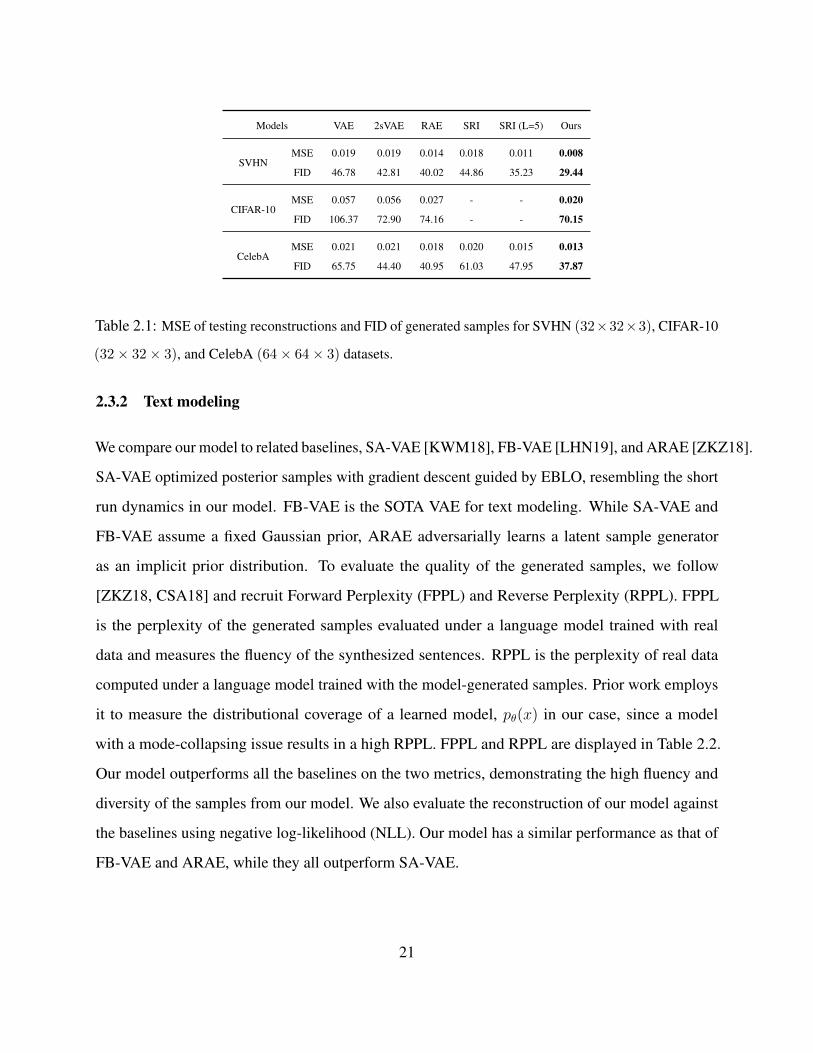
2.1 MSE of testing reconstructions and FID of generated samples for SVHN (32 × 32 × 3),

CIFAR-10 (32× 32× 3), and CelebA (64× 64× 3) datasets. . . . . . . . . . . . . . . . . 21

2.2 FPPL, RPPL, and NLL for our model and baselines on SNLI, PTB, and Yahoo datasets. . . . . 22

2.3 Transition of a Markov chain initialized from p0(z) towards pα(z). Top: Trajectory in the PTB

data-space. Each panel contains a sample for K ′0 ∈ {0, 40, 100}. Bottom: Energy profile. . . . 23

2.4 AUPRC scores for unsupervised anomaly detection on MNIST. Numbers are taken from [KGC19]

and results for our model are averaged over last 10 epochs to account for variance. . . . . . . 24

2.5 Hyperparameters for short run dynamics. . . . . . . . . . . . . . . . . . . . . . . . . 37

2.7 The sizes of word embeddings and hidden units of the generators for SNLI, PTB, and

Yahoo. . . . . . . . . . . . . . . . . . . . . . . . . . . . . . . . . . . . . . . . . . . . 38

2.8 Comparison of the models with a latent EBM prior versus a fixed Gaussian prior. The

highlighted number is the reported FID for SVHN and compared to other baseline

models in the main text. . . . . . . . . . . . . . . . . . . . . . . . . . . . . . . . . . . 39

2.9 Influence of the number of prior and posterior short run steps K0 (left) and K1 (right).

The highlighted number is the reported FID for SVHN and compared to other baseline

models in the main text. . . . . . . . . . . . . . . . . . . . . . . . . . . . . . . . . . . 39

2.10 Influence of prior and generator complexity. The highlighted number is the reported

FID for SVHN and compared to other baseline models in the main text. nef indicates

the number of hidden features of the prior EBM and ngf denotes the factor of the

number of channels of the generator (also see Table 2.6). . . . . . . . . . . . . . . . . 40

2.6 EBM model architectures for all image and text datasets and generator model architec-

tures for SVHN (32× 32× 3), CIFAR-10 (32× 32× 3), and CelebA (64× 64× 3).

. . . . . . . . . . . . . . . . . . . . . . . . . . . . . . . . . . . . . . . . . . . . . . 41

xv

3.1 Performance obtained by our model against LM-based and graph-based baselines. . . . . . . . 48

4.1 ADE / FDE metrics on Stanford Drone for LB-EBM compared to baselines are shown.

All models use 8 frames as history and predict the next 12 frames. The lower the better. 65

4.2 ADE / FDE metrics on ETH-UCY for the proposed LB-EBM and baselines are shown.

The models with * mark are non-probabilistic. All models use 8 frames as history and

predict the next 12 frames. Our model achieves the best average error on both ADE

and FDE metrics. The lower the better. . . . . . . . . . . . . . . . . . . . . . . . . . . 66

4.3 ADE / FDE metrics on Stanford Drone for different ablation conditions. The lower the

better. . . . . . . . . . . . . . . . . . . . . . . . . . . . . . . . . . . . . . . . . . . . 68

4.4 NLL Evaluation on ETH-UCY for the proposed LB-EBM and baselines are shown.

The lower the better. . . . . . . . . . . . . . . . . . . . . . . . . . . . . . . . . . . . 73

5.1 Results of language generation on PTB. . . . . . . . . . . . . . . . . . . . . . . . . . 88

5.2 Results of interpretable language generation on DD. Mutual information (MI), BLEU

and homogeneity with actions and emotions are shown. . . . . . . . . . . . . . . . . 89

5.3 Dialog evaluation results on SMD with four metrics: BLEU, average, extrema and

greedy word embedding based similarity. . . . . . . . . . . . . . . . . . . . . . . . . 90

5.4 Sample actions and corresponding utterances discovered by SVEBM-IB on SMD. . . 90

5.5 Dialog cases on SMD, which are generated by sampling dialog utterance xwith different

values of y. . . . . . . . . . . . . . . . . . . . . . . . . . . . . . . . . . . . . . . . . 91

5.6 Accuracy of sentence attribute control on Yelp. . . . . . . . . . . . . . . . . . . . . . 92

5.7 Generated positive and negative reviews with SVEBM-IB trained on Yelp. . . . . . . . 92

5.8 Semi-supervised classification accuracy on AGNews with varied number of labeled data. 93

xvi

ACKNOWLEDGMENTS

Foremost, I would like to express my sincere gratitude to my advisor Prof. Ying Nian Wu for his

encouragement, enthusiasm, patience, and guidance. His guidance on research was invaluable for

me to conduct and finish my dissertation research. His support on internship and job search is

invaluable for me to start research career after graduate school. The life wisdom I learned from him

would be invaluable for me beyond my research and career.

Besides, I would like to thank Prof. Hongquan Xu, Prof. Qing Zhou, and Prof. Mark S.

Handcock to serve on my doctoral committee. I appreciate their time on reviewing my dissertation

and attending my oral presentations. Also, thanks to them for the knowledge I learned from their

classes.

Further, I would like to thank Erik Nijkamp, Tian Han, and Wenjuan Han for thought-provoking

discussions and fruitful collaborations. Thanks to Yuhao Yin, Tianyi Sun, Shuai Zhu, Luyao Yuan

for discussions when we were taking classes together in the first years.

Finally, thanks to my wife, Han, for being there whenever I need you. Also, thanks to my

parents for their unconditional support and love.

xvii

VITA

2017–2021 Teaching Assistant, Department of Statistics, UCLA, USA.

2017 M.S. in Statistics, Texas A&M University, USA

2017 Ph.D. in Cognitive Psychology, Texas A&M University, USA

2012 B.S. in Psychology, Beijing Normal University, China

PUBLICATIONS

Pang, B. and Wu, Y. N.. Latent Space Energy-Based Model of Symbol-Vector Coupling for Text

Generation and Classification. ICML, 2021.

Pang, B., Zhao, T. Y., Xie, X., and Wu, Y. N. Trajectory Prediction with Latent Belief Energy-Based

Model. CVPR, 2021.

Pang, B., Han, T., Nijkamp, E., Zhu, S.-C., and Wu, Y. N. Learning Latent Space Energy-Based

Prior Model. NeurIPS, 2020.

Pang, B., Han, T., and Wu, Y. N. Learning Latent Space Energy-Based Prior Model for Molecule

Generation. Machine Learning for Molecules Workshop @ NeurIPS, 2020.

Pang, B., Han, T., Nijkamp, E., and Wu, Y. N. Generative Text Modeling through Short Run

Inference. EACL, 2021.

xviii

Pang, B., Han, W. J., Nijkamp, E., and Zhou, L. Q. Towards Holistic and Automatic Evaluation of

Open-Domain Dialogue Generation. ACL, 2020.

Pang, B., Nijkamp, E., and Wu, Y. N. Deep Learning with Tensorflow: A Review. Journal of

Educational and Behavioral Statistics, 2020.

Nijkamp, E., Pang, B., Wu, Y. N., and Xiong, C. M. SCRIPT: Self-Critic Pretraining of Transformers.

NAACL, 2021.

Han, W. J., Pang, B., and Wu, Y. N. Robust Transfer Learning with Pretrained Language Models

through Adapters. ACL, 2021.

Nijkamp, E., Pang, B., Han, T., and Wu, Y. N. Learning Multi-Layer Latent Variable Model via

Variational Optimization of Short Run MCMC for Approximate Inference. ECCV, 2020.

Han, T., Nijkamp, E., Zhou, L. Q., Pang, B., and Wu, Y. N. Joint Training of Variational Auto-

Encoder and Latent Energy-Based Model. CVPR, 2020.

Nijkamp, E., Gao, R. Q., Sountsov, P., Vasudevan, S., Pang, B., Zhu, S.-C., and Wu, Y. N. Learning

Energy-Based Model with Flow-Based Backbone by Neural Transport MCMC. ArXiv, 2020.

xix

CHAPTER 1

Introduction

Statistical learning or machine learning underlies many aspects of modern society: from web

searches to content filtering on social networks to recommendations on e-commerce websites,

and it is increasingly present in consumer products such as cameras and smartphones [LBH15].

The breakthroughs in the past decade, owing to the high model capacity of neural networks

and computational power of modern computing hardware, have enabled models with cognitive

capacity competitive with humans for tasks like image recognition or language understanding

[KSH12, HZR16, DCL18, BMR20]. The goal of this dissertation is to seek a simple and unified

probabilistic model and a principled learning method which, powered by the high-expressivity

modern deep neural networks and high-capacity modern computing hardware, are versatile for

modeling patterns of high dimensionality and complexity in various domains such as natural images,

natural language, and molecule graphs.

Three families of probabilistic models are widely used in modeling complex patterns. The first

class is generator models [HLZ17] which are directed top-down models and assume the observed

pattern is generated by some latent variables through a transformation. A prototype is factor analysis

[RT82], where the pattern is generated by some latent variables through a linear transformation, and

it is generalized to independent component analysis [HKO04], sparse coding [OF97], non-negative

matrix factorization [LS01], and etc. The second class is energy-based models (EBM) [DLW15,

XLZ16] which specify a probability distribution of the observed pattern via an energy function

defined on the pattern through some feature statistics extracted from the pattern. They prototype is

exponential family distributions, the Boltzmann machine [AHS85, HOT06, SH09, LGR09]. The

1

third class is discriminative models which are in the form of classifiers and specify the conditional

probability of the output class label given an input pattern.

We develop a unification of the three families of probabilistic models. The unified models retain

the advantages of the original models and avoid disadvantages of them. The unified models provide

a principled probabilistic approach to model various types of complicated patterns. In the following

sections, we introduce the background to motivate the unification and define relevant terminology.

1.1 Unifying Three Families of Probabilistic Models

1.1.1 Langevin Dynamics

Learning and inference of these probabilistic models involve MCMC. One convenient MCMC is

Langevin dynamics, which iterates

zk+1 = zk + s∇z log π(zk) +√2sϵk, (1.1)

where ϵk ∼ N(0, I), k indexes the time step of the Langevin dynamics, and s is the step size. The

Langevin dynamics consists of a gradient descent term on − log π(z) and a white noise diffusion

term√2sϵk which creates randomness for sampling from π(z).

For a small step size s, the marginal distribution of zk will converge to π(z) as k → ∞ regardless

of the initial distribution of z0. More specifically, let pk(z) be the marginal distribution of zt of

the Langevin dynamics, then DKL(pk(z)∥π(z)) decreases monotonically to 0, that is, by increasing

k, we reduce DKL(pk(z)∥π(z)) monotonically, where DKL(p∥q) indicates the Kullback–Leibler

divergence from q to p.

Convergence of Langevin dynamics to the target distribution requires infinite steps with infinites-

imal step size, which is impractical. We thus propose to use short-run MCMC [NHZ19, NHH20,

NPH19] for approximate sampling in practice. This is in agreement with the philosophy of varia-

tional inference, which accepts the intractability of the target distribution and seeks to approximate

it by a simpler distribution. The difference is that we adopt short-run Langevin dynamics instead of

2

learning a separate network for approximation.

The short-run Langevin dynamics is always initialized from the fixed initial distribution p0 such

as Gaussian noise, and only runs a fixed number of K steps, e.g., K = 20,

z0 ∼ p0(z), zk+1 = zk + s∇z log π(zk) +√2sϵk, k = 1, ..., K. (1.2)

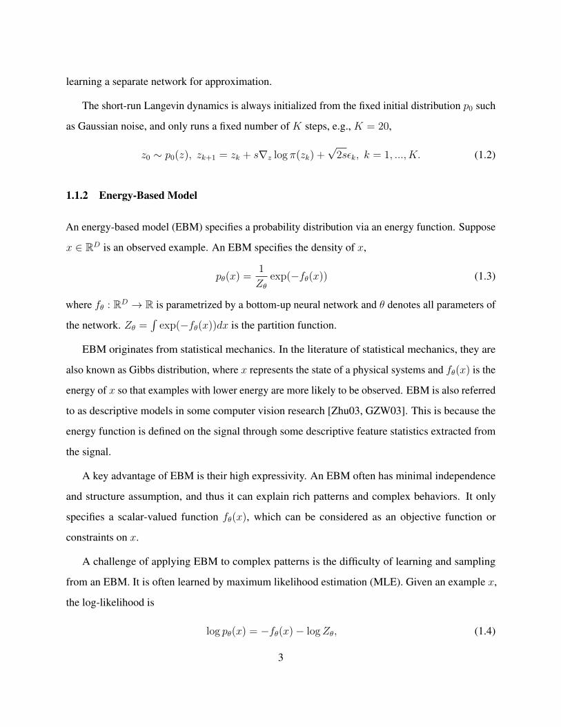
1.1.2 Energy-Based Model

An energy-based model (EBM) specifies a probability distribution via an energy function. Suppose

x ∈ RD is an observed example. An EBM specifies the density of x,

pθ(x) =1

Zθexp(−fθ(x)) (1.3)

where fθ : RD → R is parametrized by a bottom-up neural network and θ denotes all parameters of

the network. Zθ =∫exp(−fθ(x))dx is the partition function.

EBM originates from statistical mechanics. In the literature of statistical mechanics, they are

also known as Gibbs distribution, where x represents the state of a physical systems and fθ(x) is the

energy of x so that examples with lower energy are more likely to be observed. EBM is also referred

to as descriptive models in some computer vision research [Zhu03, GZW03]. This is because the

energy function is defined on the signal through some descriptive feature statistics extracted from

the signal.

A key advantage of EBM is their high expressivity. An EBM often has minimal independence

and structure assumption, and thus it can explain rich patterns and complex behaviors. It only

specifies a scalar-valued function fθ(x), which can be considered as an objective function or

constraints on x.

A challenge of applying EBM to complex patterns is the difficulty of learning and sampling

from an EBM. It is often learned by maximum likelihood estimation (MLE). Given an example x,

the log-likelihood is

log pθ(x) = −fθ(x)− logZθ, (1.4)

3

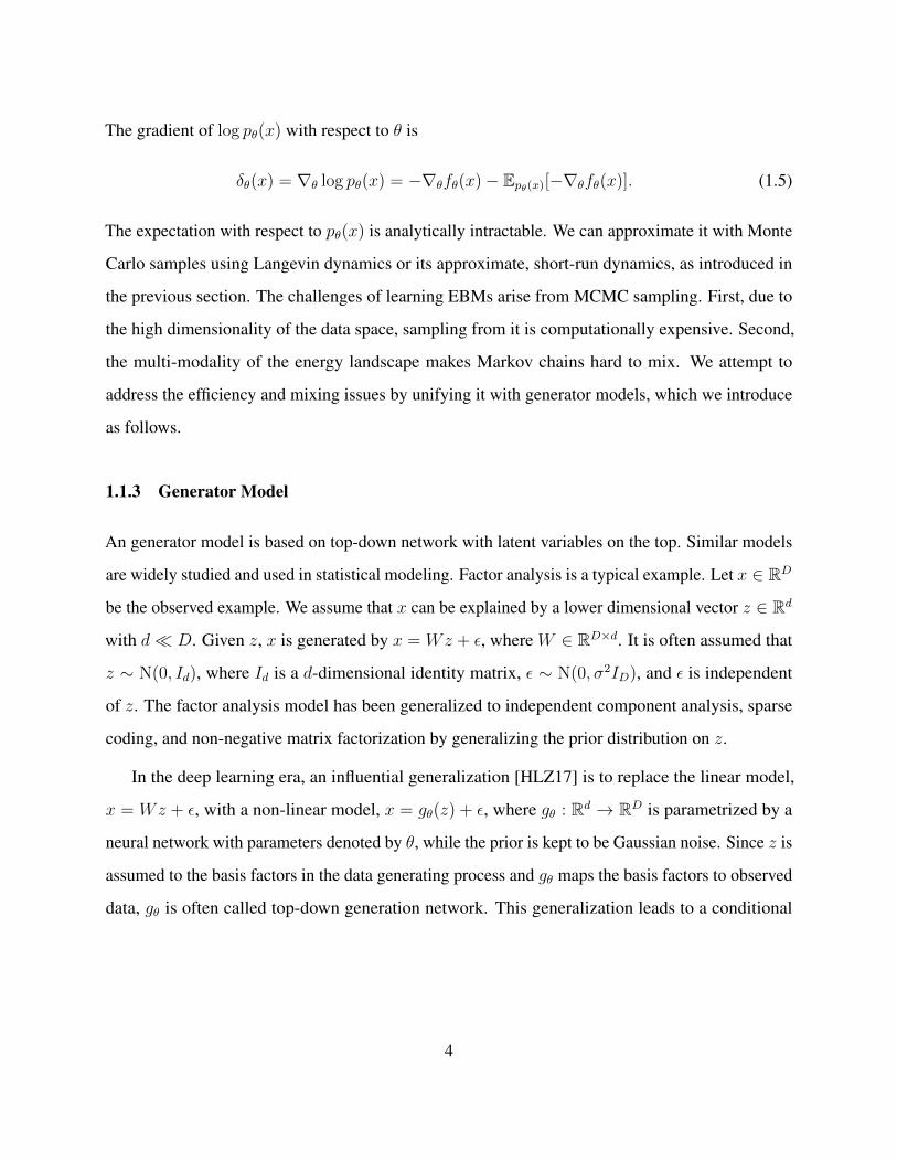
The gradient of log pθ(x) with respect to θ is

δθ(x) = ∇θ log pθ(x) = −∇θfθ(x)− Epθ(x)[−∇θfθ(x)]. (1.5)

The expectation with respect to pθ(x) is analytically intractable. We can approximate it with Monte

Carlo samples using Langevin dynamics or its approximate, short-run dynamics, as introduced in

the previous section. The challenges of learning EBMs arise from MCMC sampling. First, due to

the high dimensionality of the data space, sampling from it is computationally expensive. Second,

the multi-modality of the energy landscape makes Markov chains hard to mix. We attempt to

address the efficiency and mixing issues by unifying it with generator models, which we introduce

as follows.

1.1.3 Generator Model

An generator model is based on top-down network with latent variables on the top. Similar models

are widely studied and used in statistical modeling. Factor analysis is a typical example. Let x ∈ RD

be the observed example. We assume that x can be explained by a lower dimensional vector z ∈ Rd

with d≪ D. Given z, x is generated by x = Wz + ϵ, where W ∈ RD×d. It is often assumed that

z ∼ N(0, Id), where Id is a d-dimensional identity matrix, ϵ ∼ N(0, σ2ID), and ϵ is independent

of z. The factor analysis model has been generalized to independent component analysis, sparse

coding, and non-negative matrix factorization by generalizing the prior distribution on z.

In the deep learning era, an influential generalization [HLZ17] is to replace the linear model,

x = Wz + ϵ, with a non-linear model, x = gθ(z) + ϵ, where gθ : Rd → RD is parametrized by a

neural network with parameters denoted by θ, while the prior is kept to be Gaussian noise. Since z is

assumed to the basis factors in the data generating process and gθ maps the basis factors to observed

data, gθ is often called top-down generation network. This generalization leads to a conditional

4

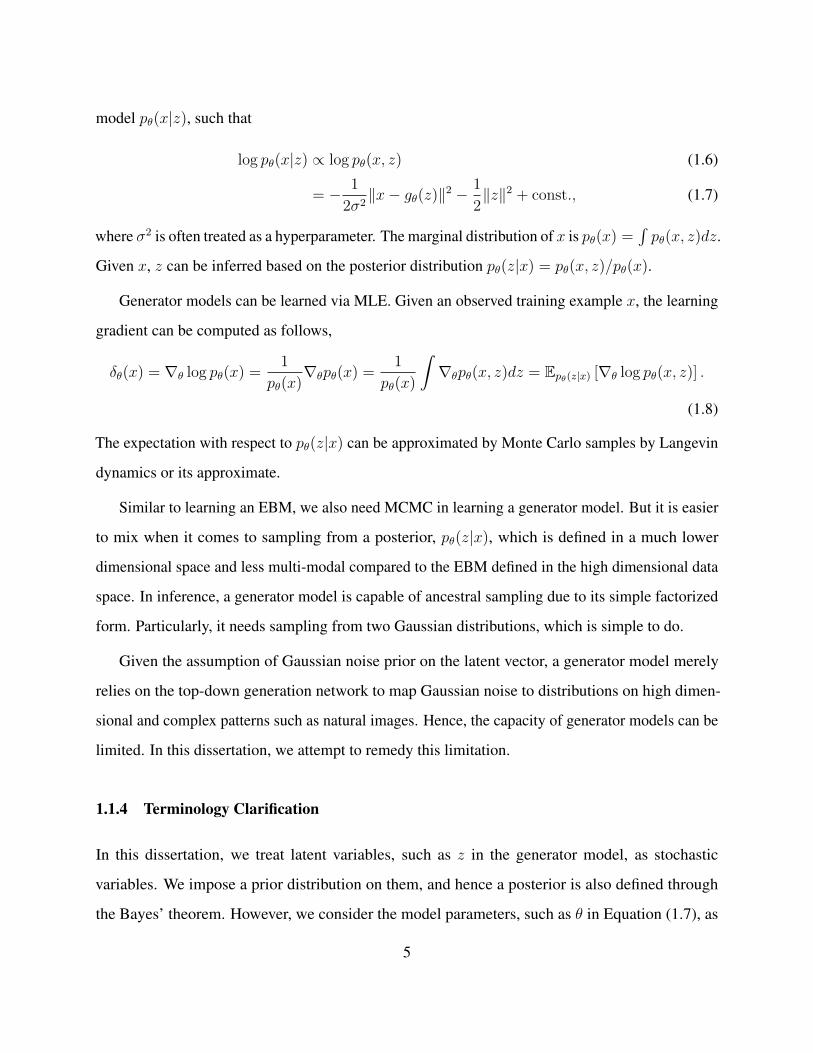
model pθ(x|z), such that

log pθ(x|z) ∝ log pθ(x, z) (1.6)

= − 1

2σ2∥x− gθ(z)∥2 −

1

2∥z∥2 + const., (1.7)

where σ2 is often treated as a hyperparameter. The marginal distribution of x is pθ(x) =∫pθ(x, z)dz.

Given x, z can be inferred based on the posterior distribution pθ(z|x) = pθ(x, z)/pθ(x).

Generator models can be learned via MLE. Given an observed training example x, the learning

gradient can be computed as follows,

δθ(x) = ∇θ log pθ(x) =1

pθ(x)∇θpθ(x) =

1

pθ(x)

∫∇θpθ(x, z)dz = Epθ(z|x) [∇θ log pθ(x, z)] .

(1.8)

The expectation with respect to pθ(z|x) can be approximated by Monte Carlo samples by Langevin

dynamics or its approximate.

Similar to learning an EBM, we also need MCMC in learning a generator model. But it is easier

to mix when it comes to sampling from a posterior, pθ(z|x), which is defined in a much lower

dimensional space and less multi-modal compared to the EBM defined in the high dimensional data

space. In inference, a generator model is capable of ancestral sampling due to its simple factorized

form. Particularly, it needs sampling from two Gaussian distributions, which is simple to do.

Given the assumption of Gaussian noise prior on the latent vector, a generator model merely

relies on the top-down generation network to map Gaussian noise to distributions on high dimen-

sional and complex patterns such as natural images. Hence, the capacity of generator models can be

limited. In this dissertation, we attempt to remedy this limitation.

1.1.4 Terminology Clarification

In this dissertation, we treat latent variables, such as z in the generator model, as stochastic

variables. We impose a prior distribution on them, and hence a posterior is also defined through

the Bayes’ theorem. However, we consider the model parameters, such as θ in Equation (1.7), as

5

a set of fixed but unknown quantities, which we attempt to estimate or learn from the observed

data through maximum likelihood estimation or its variants. Therefore, when we talk about prior

sampling and posterior sampling, they are with regard to the latent variables instead of the model

parameters. This is in contrast to the traditional Bayesian approach in which the parameters are also

treated stochastically and imposed with a prior. The Bayesian approach is also considered in the

deep learning area [GG16, GG15]. The progress is nevertheless limited by the (analytically and

computationally) intractable posterior inference due to the extremely high-dimensional parameter

space (typically on the scale of 106 to 109).

1.1.5 Unification of Generator Model and Energy-Based Model

In summary, EBM is expressive but poses challenges in sampling, while generator model is less

expressive but convenient and efficient in terms of sampling. Comparing the components instantiated

by neural networks,

Considering the benefits and drawbacks of the two models, we propose to unify the generator

model and the EBM by moving the EBM into the latent space of the generator model such that the

EBM acts as an learnable prior of the top-down generator model. Due to the low-dimensionality of

the latent space, the energy function can be parametrized by a small multi-layer perceptron, yet the

energy function can capture regularities in the data effectively and efficiently because it stands on

an expressive top-down network. Moreover, MCMC in the latent space for both prior and posterior

sampling is efficient and mixes well. We call the unified model as latent space energy-based model,

which consists of the latent space EBM prior and the top-down generation network.

1.1.6 Discriminative Model

A discriminative model specifies the conditional probability of the output class given the input

signal. Let x ∈ RD be an input example, e.g., an image or a text, and let y ∈ {1, ..., C} be the

category that x belongs to, where C is the number of categories. The commonly used softmax

6

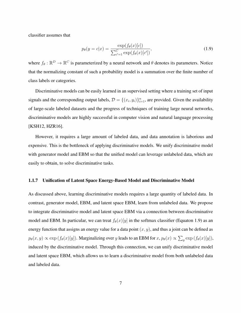
classifier assumes that

pθ(y = c|x) = exp(fθ(x)[c])∑Cc′=1 exp(fθ(x)[c

′]), (1.9)

where fθ : RD → RC is parameterized by a neural network and θ denotes its parameters. Notice

that the normalizing constant of such a probability model is a summation over the finite number of

class labels or categories.

Discriminative models can be easily learned in an supervised setting where a training set of input

signals and the corresponding output labels, D = {(xi, yi)}ni=1, are provided. Given the availability

of large-scale labeled datasets and the progress of techniques of training large neural networks,

discriminative models are highly successful in computer vision and natural language processing

[KSH12, HZR16].

However, it requires a large amount of labeled data, and data annotation is laborious and

expensive. This is the bottleneck of applying discriminative models. We unify discriminative model

with generator model and EBM so that the unified model can leverage unlabeled data, which are

easily to obtain, to solve discriminative tasks.

1.1.7 Unification of Latent Space Energy-Based Model and Discriminative Model

As discussed above, learning discriminative models requires a large quantity of labeled data. In

contrast, generator model, EBM, and latent space EBM, learn from unlabeled data. We propose

to integrate discriminative model and latent space EBM via a connection between discriminative

model and EBM. In particular, we can treat fθ(x)[y] in the softmax classifier (Equaton 1.9) as an

energy function that assigns an energy value for a data point (x, y), and thus a joint can be defined as

pθ(x, y) ∝ exp (fθ(x)[y]). Marginalizing over y leads to an EBM for x, pθ(x) ∝∑

y exp (fθ(x)[y]),

induced by the discriminative model. Through this connection, we can unify discriminative model

and latent space EBM, which allows us to learn a discriminative model from both unlabeled data

and labeled data.

7

1.2 Overview of the Dissertation

In this dissertation, we propose one approach to unify three families of probabilistic models.

Specifically, we propose to learn an EBM in the latent space of a generator model, so that the EBM

serves as a prior model that stands on the top-down network of the generator model. Due to the

low dimensionality of the latent space, a simple EBM in latent space can capture regularities in the

data effectively. The resulting model, latent space EBM, is expressive with little cost in terms of

model and computational complexity. The discriminative model is further integrated with latent

space EBM, by using a symbol-vector coupling formulation for the energy term, which couples

a continuous latent vector and a symbolic one-hot vector. Given the inferred continuous vector,

the symbol or category can be inferred from it via a standard softmax classifier. This unification

allows us to learn a classifier in a semi-supervised manner and learn well-structured and meaningful

latent space leading to a more interpretable generative model. We next give a brief overview of each

chapter.

In Chapter 2, we introduce the unification of generator model and EBM, leading to the latent

space EBM. A likelihood-based learning framework is proposed to learn the unified model. The

proposed model and learning framework lay the foundation of this dissertation. We show that this

seemingly simple integration results in rather rich applications with our principled learning method.

We apply the latent space EBM to model a variety of complex patterns including natural images

and text. Faithful and diverse samples can be sampled from the learned models, indicating that

they capture these high-dimensional and complex distributions well. Furthermore, given the good

fit, the learned models can be naturally applied to detect anomaly samples. We derive an anomaly

detection score based on the un-normalized log-posterior and achieve good performance.

In Chapter 3, we leverage the expressiveness of latent space EBM to model molecules. Various

forms can be used to encode molecules. One is simplified molecular input line entry systems

(SMILES) [Wei88] with which a molecule graph is linearized into a string consisting of characters

that represent atoms and bonds. If the molecules are encoded in this simple linear string form,

8

modeling becomes convenient. However, models relying on string representations tend to generate

invalid samples and duplicates. Prior work addressed these issues by building models on chemically-

valid fragments or explicitly enforcing chemical rules in the generation process. We argue that

an expressive model is sufficient to implicitly and automatically learn the complicated chemical

rules from the data, even if molecules are encoded in simple character-level SMILES strings. We

learn latent space EBM with SMILES representation for molecule modeling. Our experiments

show that our method is able to generate molecules with validity and uniqueness competitive with

state-of-the-art models.

In Chapter 4, we study another interesting aspect of EBM. That is, an EBM can be considered

a reward or cost function. Therefore, we can learn the cost function of experts from their demon-

strations and then learn a policy function guided by the learned cost function. This view of EBM

connects our model with inverse reinforcement learning. Levering this fact and the design of a

multi-time scale model, we propose a latent belief energy-based model for diverse human trajectory

forecast. It is a probabilistic model with cost function defined in the latent space to account for the

movement history and social context. This model achieves good performance on the challenging

benchmarks of human trajectory prediction.

In Chapter 5, building on top of the unification of generator model and EBM, we further

integrates the discriminative model into our model. To integrate the discriminative model, we recruit

an energy term of the prior model that couples a continuous latent vector and a symbolic one-hot

vector, so that discrete category can be inferred from the observed example based on the continuous

latent vector. Such a latent space coupling naturally enables incorporation of information bottleneck

regularization to encourage the continuous latent vector to extract information from the observed

example that is informative of the underlying category. In our learning method, the symbol-vector

coupling, the generator network and the inference network are learned jointly. Our model can be

learned in an unsupervised setting where no category labels are provided. It can also be learned

in semi-supervised setting where category labels are provided for a subset of training examples.

Our experiments demonstrate that the proposed model learns well-structured and meaningful latent

9

space, which (1) guides the generator to generate text with high quality, diversity, and interpretability,

and (2) effectively classifies text.

This dissertation is based on publications on latent space energy-based model [PHN20, PHW20,

PZX21, PW21]. I also published in several other areas during my graduate study [PNW20, HNZ20a,

NPH20, PNC20a, NGS20, PNH20, NPW21, HPW21] such as deep generative models, representa-

tion learning with pre-trained language models.

10

CHAPTER 2

Latent Space Energy-Based Model

2.1 Introduction

In recent years, deep generative models have achieved impressive successes in image and text

generation. A particularly simple and powerful model is the generator model [KW14, GPM14b],

which assumes that the observed example is generated by a low-dimensional latent vector via

a top-down network, and the latent vector follows a non-informative prior distribution, such as

uniform or isotropic Gaussian distribution. While we can learn an expressive top-down network

to map the prior distribution to the data distribution, we can also learn an informative prior model

in the latent space to further improve the expressive power of the whole model. This follows the

philosophy of empirical Bayes where the prior model is learned from the observed data. Specifically,

we assume the latent vector follows an energy-based model (EBM). We call this model the latent

space energy-based prior model.

Both the latent space EBM and the top-down network can be learned jointly by maximum

likelihood estimate (MLE). Each learning iteration involves Markov chain Monte Carlo (MCMC)

sampling of the latent vector from both the prior and posterior distributions. Parameters of the

prior model can then be updated based on the statistical difference between samples from the two

distributions. Parameters of the top-down network can be updated based on the samples from the

posterior distribution as well as the observed data. Due to the low-dimensionality of the latent space,

the energy function can be parametrized by a small multi-layer perceptron, yet the energy function

can capture regularities in the data effectively because the EBM stands on an expressive top-down

11

network. Moreover, MCMC in the latent space for both prior and posterior sampling is efficient

and mixes well. Specifically, we employ short-run MCMC [NHZ19, NHH20, NPH19, HLZ17]

which runs a fixed number of steps from a fixed initial distribution. We formulate the resulting

learning algorithm as a perturbation of MLE learning in terms of both objective function and

estimating equation, so that the learning algorithm has a solid theoretical foundation. Within our

theoretical framework, the short-run MCMC for posterior and prior sampling can also be amortized

by jointly learned inference and synthesis networks. However, we prefer keeping our model and

learning method pure and self-contained in the initial work (please see Chapter 4 and Chapter

5 for the employment of amortized posterior inference), without mixing in learning tricks from

variational auto-encoder (VAE) [KW14, RMW14] and generative adversarial networks (GAN)

[GPM14b, RMC16]. Thus we shall rely on short-run MCMC for simplicity.

We test the proposed modeling, learning and computing method on tasks such as image synthesis,

text generation, as well as anomaly detection. We show that our method is competitive with prior art.

The contributions of this chapter is summarized as follows. (1) We propose a latent space energy-

based prior model that stands on the top-down network of the generator model. (2) We develop

the maximum likelihood learning algorithm that learns the EBM prior and the top-down network

jointly based on MCMC sampling of the latent vector from the prior and posterior distributions.

(3) We further develop an efficient modification of MLE learning based on short-run MCMC

sampling. (4) We provide theoretical foundation for learning based on short-run MCMC. The

theoretical formulation can also be used to amortize short-run MCMC by extra inference and

synthesis networks. (5) We provide strong empirical results to illustrate the proposed method.

12

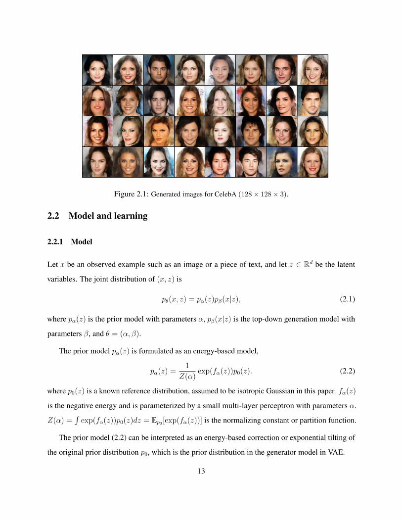
Figure 2.1: Generated images for CelebA (128× 128× 3).

2.2 Model and learning

2.2.1 Model

Let x be an observed example such as an image or a piece of text, and let z ∈ Rd be the latent

variables. The joint distribution of (x, z) is

pθ(x, z) = pα(z)pβ(x|z), (2.1)

where pα(z) is the prior model with parameters α, pβ(x|z) is the top-down generation model with

parameters β, and θ = (α, β).

The prior model pα(z) is formulated as an energy-based model,

pα(z) =1

Z(α)exp(fα(z))p0(z). (2.2)

where p0(z) is a known reference distribution, assumed to be isotropic Gaussian in this paper. fα(z)

is the negative energy and is parameterized by a small multi-layer perceptron with parameters α.

Z(α) =∫exp(fα(z))p0(z)dz = Ep0 [exp(fα(z))] is the normalizing constant or partition function.

The prior model (2.2) can be interpreted as an energy-based correction or exponential tilting of

the original prior distribution p0, which is the prior distribution in the generator model in VAE.

13

The generation model is the same as the top-down network in VAE. For image modeling,

assuming x ∈ RD,

x = gβ(z) + ϵ, (2.3)

where ϵ ∼ N(0, σ2ID), so that pβ(x|z) ∼ N(gβ(z), σ2ID). As in VAE, σ2 takes an assumed value.

For text modeling, let x = (x(t), t = 1, ..., T ) where each x(t) is a token. Following previous text

VAE model [BVV16], we define pβ(x|z) as a conditional autoregressive model,

pβ(x|z) =T∏t=1

pβ(x(t)|x(1), ..., x(t−1), z) (2.4)

which is parameterized by a recurrent network with parameters β.

In the original generator model, the top-down network gβ maps the unimodal prior distribution

p0 to be close to the usually highly multi-modal data distribution. The prior model in (2.2) refines

p0 so that gβ maps the prior model pα to be closer to the data distribution. The prior model pα does

not need to be highly multi-modal because of the expressiveness of gβ .

The marginal distribution is pθ(x) =∫pθ(x, z)dz =

∫pα(z)pβ(x|z)dz. The posterior distribu-

tion is pθ(z|x) = pθ(x, z)/pθ(x) = pα(z)pβ(x|z)/pθ(x).

In the above model, we exponentially tilt p0(z). We can also exponentially tilt p0(x, z) =

p0(z)pβ(x|z) to pθ(x, z) = 1Z(θ)

exp(fα(x, z))p0(x, z). Equivalently, we may also exponentially tilt

p0(z, ϵ) = p0(z)p(ϵ), as the mapping from (z, ϵ) to (z, x) is a change of variable. This leads to an

EBM in both the latent space and data space, which makes learning and sampling more complex.

Therefore, we choose to only tilt p0(z) and leave pβ(x|z) as a directed top-down generation model.

2.2.2 Maximum likelihood

Suppose we observe training examples (xi, i = 1, ..., n). The log-likelihood function is

L(θ) =n∑i=1

log pθ(xi). (2.5)

14

The learning gradient can be calculated according to

∇θ log pθ(x) = Epθ(z|x) [∇θ log pθ(x, z)] = Epθ(z|x) [∇θ(log pα(z) + log pβ(x|z))] . (2.6)

See Theoretical derivations in the Supplementary for a detailed derivation.

For the prior model, ∇α log pα(z) = ∇αfα(z)− Epα(z)[∇αfα(z)]. Thus the learning gradient

for an example x is

δα(x) = ∇α log pθ(x) = Epθ(z|x)[∇αfα(z)]− Epα(z)[∇αfα(z)]. (2.7)

The above equation has an empirical Bayes nature. pθ(z|x) is based on the empirical observation x,

while pα is the prior model. α is updated based on the difference between z inferred from empirical

observation x, and z sampled from the current prior.

For the generation model,

δβ(x) = ∇β log pθ(x) = Epθ(z|x)[∇β log pβ(x|z)], (2.8)

where log pβ(x|z) = −∥x−gβ(z)∥2/(2σ2)+const or∑T

t=1 log pβ(x(t)|x(1), ..., x(t−1), z) for image

and text modeling respectively.

Expectations in (2.7) and (2.8) require MCMC sampling of the prior model pα(z) and the

posterior distribution pθ(z|x). We can use Langevin dynamics [Nea11, ZM98]. For a target

distribution π(z), the dynamics iterates zk+1 = zk + s∇z log π(zk) +√2sϵk, where k indexes the

time step of the Langevin dynamics, s is a small step size, and ϵk ∼ N(0, Id) is the Gaussian white

noise. π(z) can be either pα(z) or pθ(z|x). In either case, ∇z log π(z) can be efficiently computed

by back-propagation.

2.2.3 Short-run MCMC

As we discussed in Chapter 1, convergence of Langevin dynamics to the target distribution requires

infinite steps with infinitesimal step size, which is impractical. We thus propose to use short-run

MCMC [NHZ19, NHH20, NPH19] for approximate sampling.

15

The short-run Langevin dynamics is always initialized from the fixed initial distribution p0, and

only runs a fixed number of K steps, e.g., K = 20,

z0 ∼ p0(z), zk+1 = zk + s∇z log π(zk) +√2sϵk, k = 1, ..., K. (2.9)

Denote the distribution of zK to be π(z). Because of fixed p0(z) and fixed K and s, the distribution

π is well defined. In this paper, we put ˜ sign on top of the symbols to denote distributions or

quantities produced by short-run MCMC, and for simplicity, we omit the dependence on K and s

in notation. As shown in [CT06], the Kullback-Leibler divergence DKL(π∥π) decreases to zero

monotonically as K → ∞.

Specifically, denote the distribution of zK to be pα(z) if the target π(z) = pα(z), and denote the

distribution of zK to be pθ(z|x) if π(z) = pθ(z|x). We can then replace pα(z) by pα(z) and replace

pθ(z|x) by pθ(z|x) in equations (2.7) and (2.8), so that the learning gradients in equations (2.7) and

(2.8) are modified to

δα(x) = Epθ(z|x)[∇αfα(z)]− Epα(z)[∇αfα(z)], (2.10)

δβ(x) = Epθ(z|x)[∇β log pβ(x|z)]. (2.11)

We then update α and β based on (2.10) and (2.11), where the expectations can be approximated by

Monte Carlo samples.

2.2.4 Algorithm

The learning and sampling algorithm is described in Algorithm 1. Note that the posterior sampling

and prior sampling correspond to the positive phase and negative phase of latent EBM [AHS85].

2.2.5 Theoretical understanding

The learning algorithm based on short-run MCMC sampling in Algorithm 1 is a modification or

perturbation of maximum likelihood learning, where we replace pα(z) and pθ(z|x) by pα(z) and

16

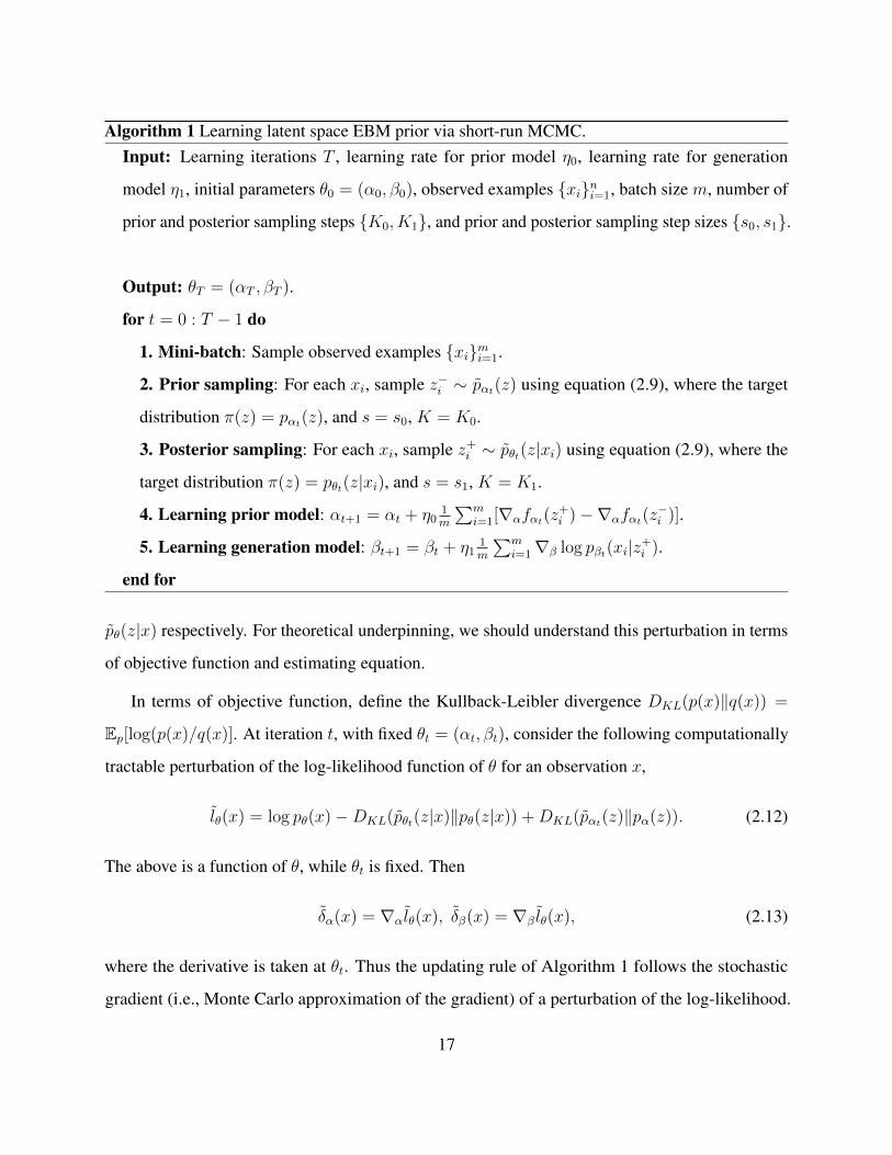
Algorithm 1 Learning latent space EBM prior via short-run MCMC.Input: Learning iterations T , learning rate for prior model η0, learning rate for generation

model η1, initial parameters θ0 = (α0, β0), observed examples {xi}ni=1, batch size m, number of

prior and posterior sampling steps {K0, K1}, and prior and posterior sampling step sizes {s0, s1}.

Output: θT = (αT , βT ).

for t = 0 : T − 1 do

1. Mini-batch: Sample observed examples {xi}mi=1.

2. Prior sampling: For each xi, sample z−i ∼ pαt(z) using equation (2.9), where the target

distribution π(z) = pαt(z), and s = s0, K = K0.

3. Posterior sampling: For each xi, sample z+i ∼ pθt(z|xi) using equation (2.9), where the

target distribution π(z) = pθt(z|xi), and s = s1, K = K1.

4. Learning prior model: αt+1 = αt + η01m

∑mi=1[∇αfαt(z

+i )−∇αfαt(z

−i )].

5. Learning generation model: βt+1 = βt + η11m

∑mi=1∇β log pβt(xi|z+i ).

end for

pθ(z|x) respectively. For theoretical underpinning, we should understand this perturbation in terms

of objective function and estimating equation.

In terms of objective function, define the Kullback-Leibler divergence DKL(p(x)∥q(x)) =

Ep[log(p(x)/q(x)]. At iteration t, with fixed θt = (αt, βt), consider the following computationally

tractable perturbation of the log-likelihood function of θ for an observation x,

lθ(x) = log pθ(x)−DKL(pθt(z|x)∥pθ(z|x)) +DKL(pαt(z)∥pα(z)). (2.12)

The above is a function of θ, while θt is fixed. Then

δα(x) = ∇αlθ(x), δβ(x) = ∇β lθ(x), (2.13)

where the derivative is taken at θt. Thus the updating rule of Algorithm 1 follows the stochastic

gradient (i.e., Monte Carlo approximation of the gradient) of a perturbation of the log-likelihood.

17

Because θt is fixed, we can drop the entropies of pθt(z|x) and pαt(z) in the above Kullback-Leibler

divergences, hence the updating rule follows the stochastic gradient of

Q(θ) = L(θ) +n∑i=1

[Epθt (zi|xi)[log pθ(zi|xi)]− Epαt (z)[log pα(z)]

], (2.14)

where L(θ) is the total log-likelihood defined in equation (2.5), and the gradient is taken at θt.

In equation (2.12), the first DKL term is related to the EM algorithm [DLR77]. It leads to

the more tractable complete-data log-likelihood. The second DKL term is related to contrastive

divergence [Tie08], except that the short-run MCMC for pαt(z) is initialized from p0(z). It serves

to cancel the intractable logZ(α) term.

In terms of estimating equation, the stochastic gradient descent in Algorithm 1 is a Robbins-

Monro stochastic approximation algorithm [RM51] that solves the following estimating equation:

1

n

n∑i=1

δα(xi) =1

n

n∑i=1

Epθ(zi|xi)[∇αfα(zi)]− Epα(z)[∇αfα(z)] = 0, (2.15)

1

n

n∑i=1

δβ(xi) =1

n

n∑i=1

Epθ(zi|xi)[∇β log pβ(xi|zi)] = 0. (2.16)

The solution to the above estimating equation defines an estimator of the parameters. Algorithm 1

converges to this estimator under the usual regularity conditions of Robbins-Monro [RM51]. If we

replace pα(z) by pα(z), and pθ(z|x) by pθ(z|x), then the above estimating equation is the maximum

likelihood estimating equation.

2.2.6 Amortized inference and synthesis

We can amortize the short-run MCMC sampling of the prior and posterior distributions of the latent

vector by jointly learning an extra inference network qϕ(z|x) and an extra synthesis network qψ(z),

together with the original model. Let us re-define lθ(x) in (2.12) by

lθ,ϕ,ψ(x) = log pθ(x)−DKL(qϕ(z|x)∥pθ(z|x)) +DKL(qψ(z)∥pα(z)), (2.17)

where we replace pθt(z|x) in (2.12) by qϕ(z|x) and replace pαt(z) in (2.12) by qψ(z). See [HNF19a,

HNZ20b] for related formulations. Define L(θ, ϕ, ψ) = 1n

∑ni=1 lθ,ϕ,ψ(x), we can jointly learn

18

(θ, ϕ, ψ) by maxθ,ϕminψ L(θ, ϕ, ψ). The objective function L(θ, ϕ, ψ) is a perturbation of the

log-likelihood L(θ) in (2.5), where −DKL(qϕ(z|x)∥pθ(z|x)) leads to variational learning, and the

learning of the inference network qϕ(z|x) follows VAE, except that we include the EBM prior

log pα(z) in training qϕ(z|x) (logZ(α) can be discarded as a constant relative to ϕ). The synthesis

network qψ(z) can be taken to be a flow-based model [DSB17, RM15]. DKL(qψ(z)∥pα(z)) leads

to adversarial training of qψ(z) and pα(z). qψ(z) is trained as a variational approximation to pα(z)

(again logZ(α) can be discarded as a constant relative to ψ), while pα(z) is updated based on

statistical difference between samples from the approximate posterior qϕ(z|x) and samples from

the approximate prior qψ(z), i.e., pα(z) is a critic of qψ(z). See supplementary materials for a

formulation based on three DKL terms.

In this initial work, we prefer keeping our model and learning method clean and simple, without

involving extra networks for learned computations, and without mixing in learning tricks from VAE

and GAN. See our follow-up work on joint training of amortized inference network [PNC20b]. See

also [XLG18] for a temporal difference MCMC teaching scheme for amortizing MCMC.

2.3 Experiments

We present a set of experiments which highlight the effectiveness of our proposed model with (1)

excellent synthesis for both visual and textual data outperforming state-of-the-art baselines, (2) high

expressiveness of the learned prior model for both data modalities, and (3) strong performance in

anomaly detection. For image data, we include SVHN [NWC11], CelebA [LLW15], and CIFAR-

10 [KNH]. For text data, we include PTB [MMS93], Yahoo [YHS17], and SNLI [BAP15].

2.3.1 Image modeling

We evaluate the quality of the generated and reconstructed images. If the model is well-learned,

the latent space EBM πα(z) will fit the generator posterior pθ(z|x) which in turn renders realistic

generated samples as well as faithful reconstructions. We compare our model with VAE [KW14]

19

and SRI [NHZ19] which assume a fixed Gaussian prior distribution for the latent vector and two

recent strong VAE variants, 2sVAE [DW19a] and RAE [GSV20], whose prior distributions are

learned with posterior samples in a second stage. We also compare with multi-layer generator (i.e.,

5 layers of latent vectors) model [NHZ19] which admits a powerful learned prior on the bottom

layer of latent vector. We follow the protocol as in [NHZ19].

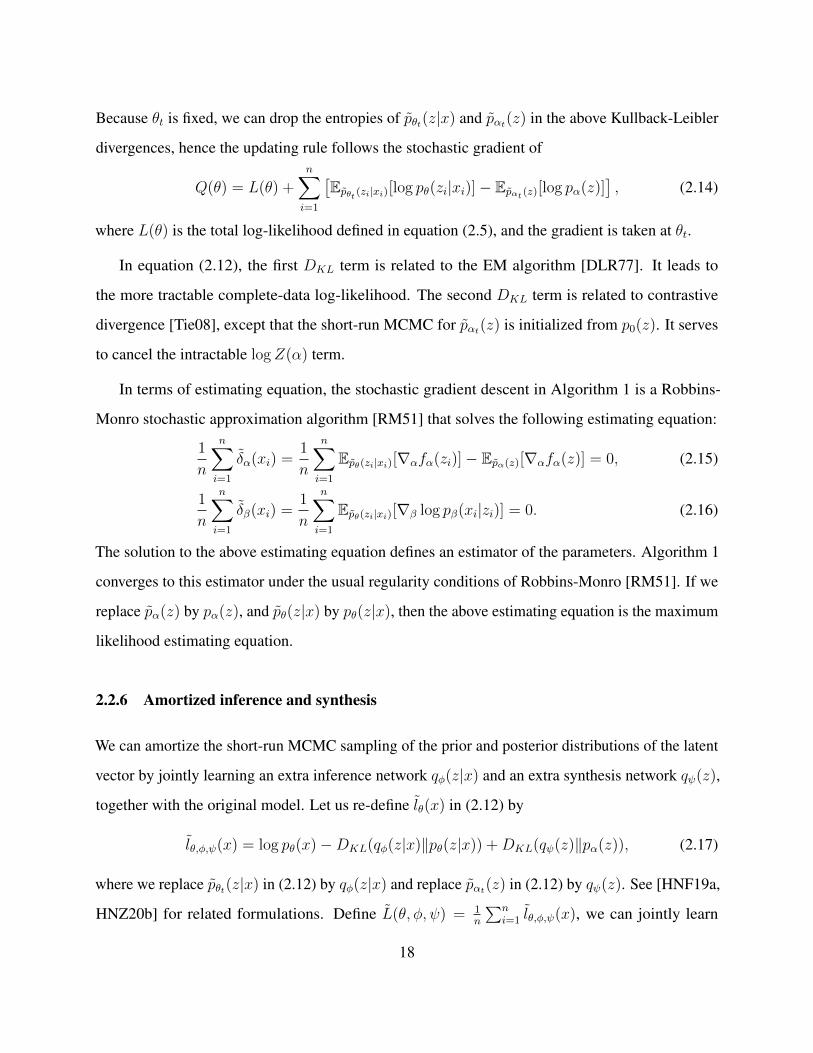
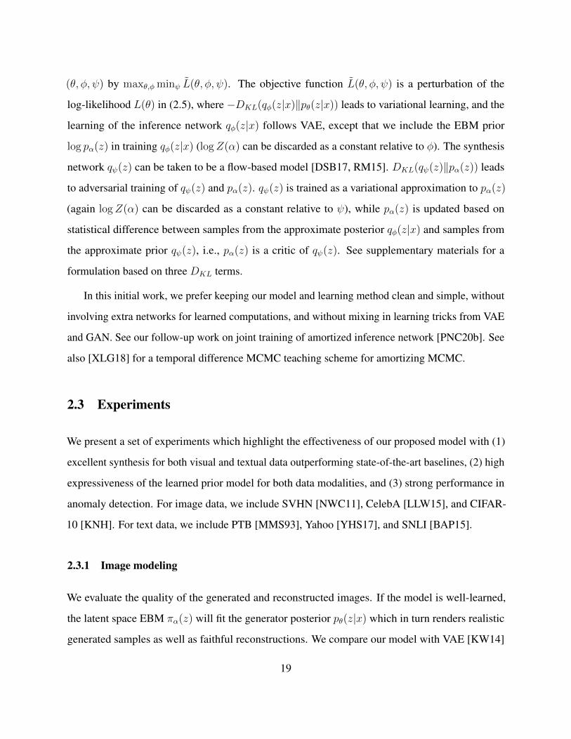
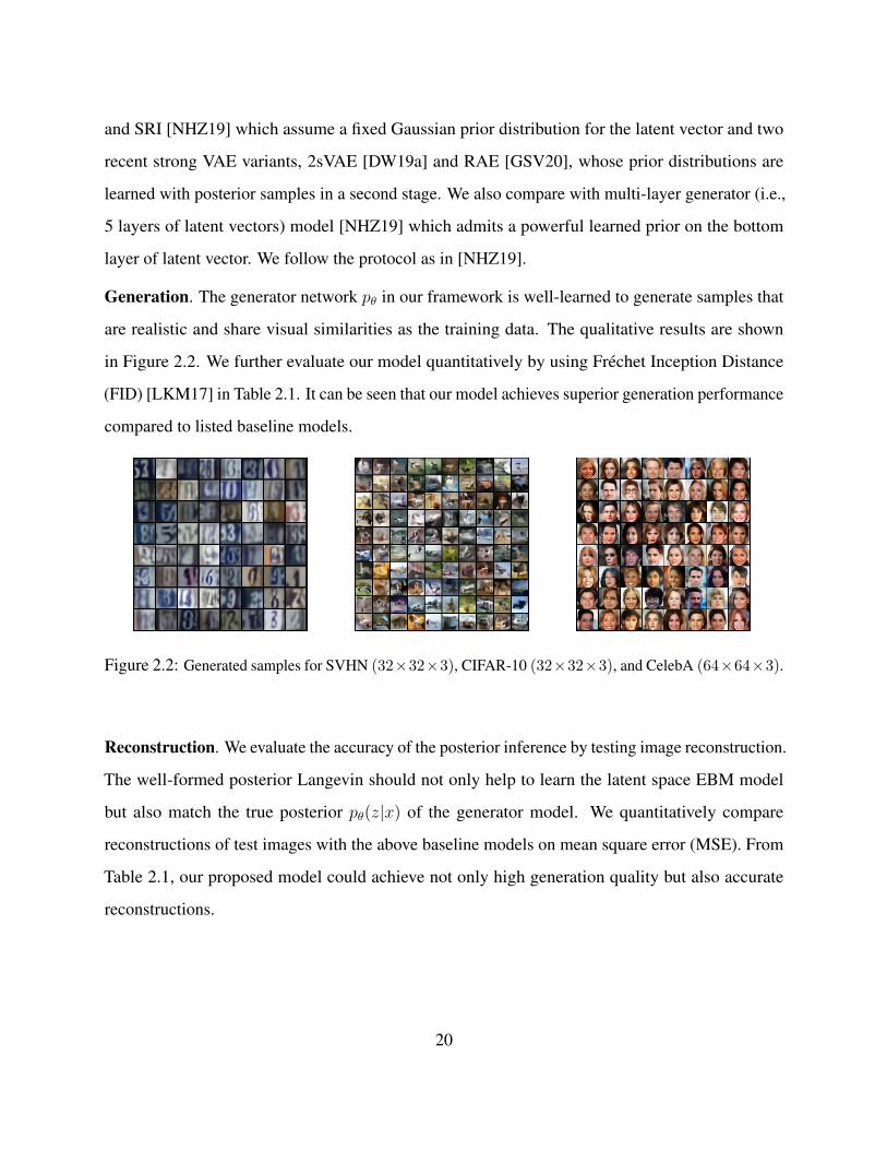
Generation. The generator network pθ in our framework is well-learned to generate samples that

are realistic and share visual similarities as the training data. The qualitative results are shown

in Figure 2.2. We further evaluate our model quantitatively by using Frechet Inception Distance

(FID) [LKM17] in Table 2.1. It can be seen that our model achieves superior generation performance

compared to listed baseline models.

Figure 2.2: Generated samples for SVHN (32×32×3), CIFAR-10 (32×32×3), and CelebA (64×64×3).

Reconstruction. We evaluate the accuracy of the posterior inference by testing image reconstruction.

The well-formed posterior Langevin should not only help to learn the latent space EBM model

but also match the true posterior pθ(z|x) of the generator model. We quantitatively compare

reconstructions of test images with the above baseline models on mean square error (MSE). From

Table 2.1, our proposed model could achieve not only high generation quality but also accurate

reconstructions.

20

Models VAE 2sVAE RAE SRI SRI (L=5) Ours

SVHNMSE 0.019 0.019 0.014 0.018 0.011 0.008

FID 46.78 42.81 40.02 44.86 35.23 29.44

CIFAR-10MSE 0.057 0.056 0.027 - - 0.020

FID 106.37 72.90 74.16 - - 70.15

CelebAMSE 0.021 0.021 0.018 0.020 0.015 0.013

FID 65.75 44.40 40.95 61.03 47.95 37.87

Table 2.1: MSE of testing reconstructions and FID of generated samples for SVHN (32×32×3), CIFAR-10

(32× 32× 3), and CelebA (64× 64× 3) datasets.

2.3.2 Text modeling

We compare our model to related baselines, SA-VAE [KWM18], FB-VAE [LHN19], and ARAE [ZKZ18].

SA-VAE optimized posterior samples with gradient descent guided by EBLO, resembling the short

run dynamics in our model. FB-VAE is the SOTA VAE for text modeling. While SA-VAE and

FB-VAE assume a fixed Gaussian prior, ARAE adversarially learns a latent sample generator

as an implicit prior distribution. To evaluate the quality of the generated samples, we follow

[ZKZ18, CSA18] and recruit Forward Perplexity (FPPL) and Reverse Perplexity (RPPL). FPPL

is the perplexity of the generated samples evaluated under a language model trained with real

data and measures the fluency of the synthesized sentences. RPPL is the perplexity of real data

computed under a language model trained with the model-generated samples. Prior work employs

it to measure the distributional coverage of a learned model, pθ(x) in our case, since a model

with a mode-collapsing issue results in a high RPPL. FPPL and RPPL are displayed in Table 2.2.

Our model outperforms all the baselines on the two metrics, demonstrating the high fluency and

diversity of the samples from our model. We also evaluate the reconstruction of our model against

the baselines using negative log-likelihood (NLL). Our model has a similar performance as that of

FB-VAE and ARAE, while they all outperform SA-VAE.

21

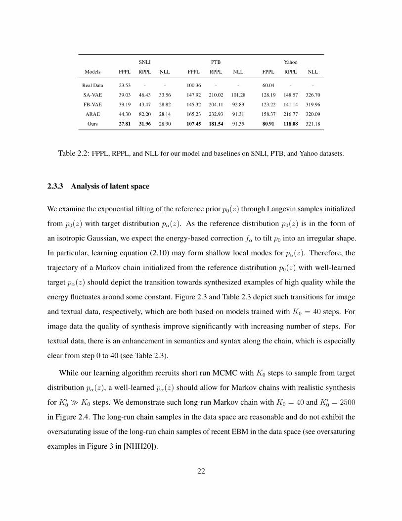
SNLI PTB Yahoo

Models FPPL RPPL NLL FPPL RPPL NLL FPPL RPPL NLL

Real Data 23.53 - - 100.36 - - 60.04 - -

SA-VAE 39.03 46.43 33.56 147.92 210.02 101.28 128.19 148.57 326.70

FB-VAE 39.19 43.47 28.82 145.32 204.11 92.89 123.22 141.14 319.96

ARAE 44.30 82.20 28.14 165.23 232.93 91.31 158.37 216.77 320.09

Ours 27.81 31.96 28.90 107.45 181.54 91.35 80.91 118.08 321.18

Table 2.2: FPPL, RPPL, and NLL for our model and baselines on SNLI, PTB, and Yahoo datasets.

2.3.3 Analysis of latent space

We examine the exponential tilting of the reference prior p0(z) through Langevin samples initialized

from p0(z) with target distribution pα(z). As the reference distribution p0(z) is in the form of

an isotropic Gaussian, we expect the energy-based correction fα to tilt p0 into an irregular shape.

In particular, learning equation (2.10) may form shallow local modes for pα(z). Therefore, the

trajectory of a Markov chain initialized from the reference distribution p0(z) with well-learned

target pα(z) should depict the transition towards synthesized examples of high quality while the

energy fluctuates around some constant. Figure 2.3 and Table 2.3 depict such transitions for image

and textual data, respectively, which are both based on models trained with K0 = 40 steps. For

image data the quality of synthesis improve significantly with increasing number of steps. For

textual data, there is an enhancement in semantics and syntax along the chain, which is especially

clear from step 0 to 40 (see Table 2.3).

While our learning algorithm recruits short run MCMC with K0 steps to sample from target

distribution pα(z), a well-learned pα(z) should allow for Markov chains with realistic synthesis

for K ′0 ≫ K0 steps. We demonstrate such long-run Markov chain with K0 = 40 and K ′

0 = 2500

in Figure 2.4. The long-run chain samples in the data space are reasonable and do not exhibit the

oversaturating issue of the long-run chain samples of recent EBM in the data space (see oversaturing

examples in Figure 3 in [NHH20]).

22

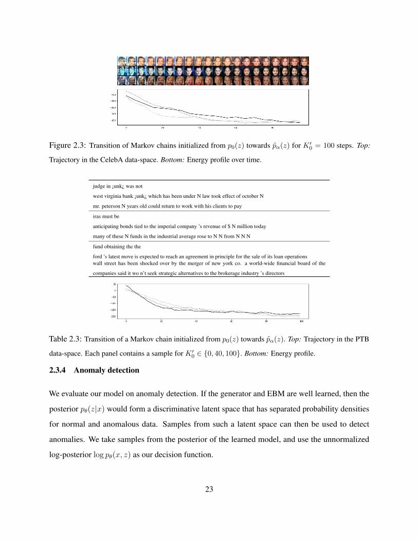
Figure 2.3: Transition of Markov chains initialized from p0(z) towards pα(z) for K ′0 = 100 steps. Top:

Trajectory in the CelebA data-space. Bottom: Energy profile over time.

judge in ¡unk¿ was not

west virginia bank ¡unk¿ which has been under N law took effect of october N

mr. peterson N years old could return to work with his clients to pay

iras must be

anticipating bonds tied to the imperial company ’s revenue of $ N million today

many of these N funds in the industrial average rose to N N from N N N

fund obtaining the the

ford ’s latest move is expected to reach an agreement in principle for the sale of its loan operationswall street has been shocked over by the merger of new york co. a world-wide financial board of the

companies said it wo n’t seek strategic alternatives to the brokerage industry ’s directors

Table 2.3: Transition of a Markov chain initialized from p0(z) towards pα(z). Top: Trajectory in the PTB

data-space. Each panel contains a sample for K ′0 ∈ {0, 40, 100}. Bottom: Energy profile.

2.3.4 Anomaly detection

We evaluate our model on anomaly detection. If the generator and EBM are well learned, then the

posterior pθ(z|x) would form a discriminative latent space that has separated probability densities

for normal and anomalous data. Samples from such a latent space can then be used to detect

anomalies. We take samples from the posterior of the learned model, and use the unnormalized

log-posterior log pθ(x, z) as our decision function.

23

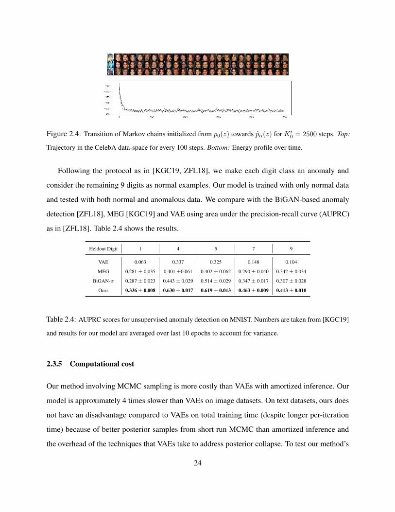
Figure 2.4: Transition of Markov chains initialized from p0(z) towards pα(z) for K ′0 = 2500 steps. Top:

Trajectory in the CelebA data-space for every 100 steps. Bottom: Energy profile over time.

Following the protocol as in [KGC19, ZFL18], we make each digit class an anomaly and

consider the remaining 9 digits as normal examples. Our model is trained with only normal data

and tested with both normal and anomalous data. We compare with the BiGAN-based anomaly

detection [ZFL18], MEG [KGC19] and VAE using area under the precision-recall curve (AUPRC)

as in [ZFL18]. Table 2.4 shows the results.

Heldout Digit 1 4 5 7 9

VAE 0.063 0.337 0.325 0.148 0.104

MEG 0.281 ± 0.035 0.401 ±0.061 0.402 ± 0.062 0.290 ± 0.040 0.342 ± 0.034

BiGAN-σ 0.287 ± 0.023 0.443 ± 0.029 0.514 ± 0.029 0.347 ± 0.017 0.307 ± 0.028

Ours 0.336 ± 0.008 0.630 ± 0.017 0.619 ± 0.013 0.463 ± 0.009 0.413 ± 0.010

Table 2.4: AUPRC scores for unsupervised anomaly detection on MNIST. Numbers are taken from [KGC19]

and results for our model are averaged over last 10 epochs to account for variance.

2.3.5 Computational cost

Our method involving MCMC sampling is more costly than VAEs with amortized inference. Our

model is approximately 4 times slower than VAEs on image datasets. On text datasets, ours does

not have an disadvantage compared to VAEs on total training time (despite longer per-iteration

time) because of better posterior samples from short run MCMC than amortized inference and

the overhead of the techniques that VAEs take to address posterior collapse. To test our method’s

24

scalability, we trained a larger generator on CelebA (128× 128). It produced faithful samples (see

Figure 2.1).

2.4 Discussion and conclusion

2.4.1 Modeling strategies and related work

We now put our work within the bigger picture of modeling and learning, and discuss related work.

Energy-based model and top-down generation model. A top-down model or a directed acyclic

graphical model is of a simple factorized form that is capable of ancestral sampling. The prototype

of such a model is factor analysis [RT82], which has been generalized to independent component

analysis [HKO04], sparse coding [OF97], non-negative matrix factorization [LS01], etc. An early

example of a multi-layer top-down model is the generation model of Helmholtz machine [HDF95].

An EBM defines an unnormalized density or a Gibbs distribution. The prototypes of such a model

are exponential family distribution, the Boltzmann machine [AHS85, HOT06, SH09, LGR09], and

the FRAME (Filters, Random field, And Maximum Entropy) model [ZWM98a]. [Zhu03] contrasted

these two classes of models, calling the top-down latent variable model the generative model, and

the energy-based model the descriptive model. [GZW03] proposed to integrate the two models,

where the top-down generation model generates textons, while the EBM prior accounts for the

perceptual organization or Gestalt laws of textons. Our model follows such a plan. Recently, DVAEs

[Rol16, VMB18, VAM18] adopted restricted Boltzmann machines as the prior model for binary

latent variables and a deep neural network as the top-down generation model.

The energy-based model can be translated into a classifier and vice versa via the Bayes rule

[GH10, Tu07, DLW15, XLZ16, JLT17, LJT17, GNK20, GWJ19, PNC20b]. The energy function

in the EBM can be viewed as an objective function, a cost function, or a critic [SB18]. It captures

regularities, rules or constrains. It is easy to specify, although optimizing or sampling the energy

function requires iterative computation such as MCMC. The maximum likelihood learning of EBM

25

can be interpreted as an adversarial scheme [XZW17, XZG18, WGH19, HNZ20b, FCA16], where

the MCMC serves as a generator or an actor and the energy function serves as an evaluator or a

critic. The top-down generation model can be viewed as an actor [SB18] that directly generates

samples. It is easy to sample from, though a complex top-down model is necessary for high quality

samples. Comparing the two models, the scalar-valued energy function can be more expressive

than the vector-valued top-down network of the same complexity, while the latter is much easier to

sample from. It is thus desirable to let EBM take over the top layers of the top-down model to make

it more expressive and make EBM learning feasible.

Energy-based correction of top-down model. The top-down model usually assumes inde-

pendent nodes at the top layer and conditional independent nodes at subsequent layers. We can

introduce energy terms at multiple layers to correct the independence or conditional independence

assumptions, and to introduce inductive biases. This leads to a latent energy-based model. However,

unlike undirected latent EBM, the energy-based correction is learned on top of a directed top-down

model, and this can be easier than learning an undirected latent EBM from scratch. Our work is

a simple example of this strategy where we correct the prior distribution. We can also correct the

generation model in the data space.

From data space EBM to latent space EBM. EBM learned in data space such as image

space [NCK11, LZW16, XLZ16, GLZ18, HNF19b, NHZ19, DM19] can be highly multi-modal,

and MCMC sampling can be difficult. We can introduce latent variables and learn an EBM in latent

space, while also learning a mapping from the latent space to the data space. Our work follows

such a strategy. Earlier papers on this strategy are [Zhu03, GZW03, BMD13, BDS18, KGC19].

Learning EBM in latent space can be much more feasible than in data space in terms of MCMC

sampling, and much of past work on EBM can be recast in the latent space.

Short-run MCMC and amortized computation. Recently, [NHZ19] proposed to use short-run

MCMC to sample from the EBM in data space. [NPH19] used it to sample the latent variables

of a top-down generation model from their posterior distribution. [Hof17] used it to improve the

posterior samples from an inference network. Our work adopts short-run MCMC to sample from

26

both the prior and the posterior of the latent variables. We provide theoretical foundation for the

learning algorithm with short-run MCMC sampling. Our theoretical formulation can also be used to

jointly train networks that amortize the MCMC sampling from the posterior and prior distributions.

Generator model with flexible prior. The expressive power of the generator network for image

and text generation comes from the top-down network that maps a simple prior to be close to the

data distribution. Most of the existing papers [MSJ15, TBG17, ACB17, DAB17, THF19, KGC19]

assume that the latent vector follows a given simple prior, such as isotropic Gaussian distribution

or uniform distribution. However, such assumption may cause ineffective generator learning as

observed in [DW19b, TW18b]. Some VAE variants attempted to address the mismatch between

the prior and the aggregate posterior. VampPrior [TW18a] parameterized the prior based on the

posterior inference model, while [BM19] proposed to construct priors using rejection sampling.

ARAE [ZKZ18] learned an implicit prior with adversarial training. Recently, some papers used

two-stage approach [DW19a, GSV20]. They first trained a VAE or deterministic auto-encoder. To

enable generation from the model, they fitted a VAE or Gaussian mixture to the posterior samples

from the first-stage model. VQ-VAE [VV17] adopted a similar approach and an autoregressive

distribution over z was learned from the posterior samples. All of these prior models generally

follow the empirical Bayes philosophy, which is also one motivation of our work.

2.4.2 Conclusion

EBM has many applications, however, its soundness and its power are limited by the difficulty with

MCMC sampling. By moving from data space to latent space, and letting the EBM stand on an

expressive top-down network, MCMC-based learning of EBM becomes sound and feasible, and

EBM in latent space can capture regularities in data effectively. We may unleash the power of EBM

in the latent space for many applications.

27

CHAPTER APPENDIX

2.A Theoretical derivations

In this section, we shall derive most of the equations in the main text. We take a step by step

approach, starting from simple identities or results, and gradually reaching the main results. Our

derivations are unconventional, but they pertain more to our model and learning method.

2.A.1 A simple identity

Let x ∼ pθ(x). A useful identity is

Eθ[∇θ log pθ(x)] = 0, (2.18)

where Eθ (or Epθ) is the expectation with respect to pθ.

The proof is one liner:

Eθ[∇θ log pθ(x)] =

∫[∇θ log pθ(x)]pθ(x)dx =

∫∇θpθ(x)dx = ∇θ

∫pθ(x)dx = ∇θ1 = 0.

(2.19)

The above identity has generalized versions, such as the one underlying the policy gradi-

ent [Wil92, SMS00], ∇θ Eθ[R(x)] = Eθ[R(x)∇θ log pθ(x)]. By letting R(x) = 1, we get (2.18).

2.A.2 Maximum likelihood estimating equation

The simple identity (2.18) also underlies the consistency of MLE. Suppose we observe (xi, i =

1, ..., n) ∼ pθtrue(x) independently, where θtrue is the true value of θ. The log-likelihood is

L(θ) =1

n

n∑i=1

log pθ(xi). (2.20)

The maximum likelihood estimating equation is

L′(θ) =1

n

n∑i=1

∇θ log pθ(xi) = 0. (2.21)

28

According to the law of large number, as n→ ∞, the above estimating equation converges to

Eθtrue [∇θ log pθ(x)] = 0, (2.22)

where θ is the unknown value to be solved, while θtrue is fixed. According to the simple identity

(2.18), θ = θtrue is the solution to the above estimating equation (2.22), no matter what θtrue is.

Thus with regularity conditions, such as identifiability of the model, the MLE converges to θtrue in

probability.

The optimality of the maximum likelihood estimating equation among all the asymptotically

unbiased estimating equations can be established based on a further generalization of the simple

identity (2.18).

We shall justify our learning method with short-run MCMC in terms of an estimating equation,

which is a perturbation of the maximum likelihood estimating equation (2.21).

2.A.3 MLE learning gradient for θ

Recall that pθ(x, z) = pα(z)pβ(x|z), where θ = {α, β}. The learning gradient for an observation x

is as follows:

∇θ log pθ(x) = Epθ(z|x) [∇θ log pθ(x, z)] = Epθ(z|x) [∇θ(log pα(z) + log pβ(x|z))] . (2.23)

The above identity is a simple consequence of the simple identity (2.18).

Epθ(z|x) [∇θ log pθ(x, z)] = Epθ(z|x) [∇θ log pθ(z|x) +∇θ log pθ(x)] (2.24)

= Epθ(z|x) [∇θ log pθ(z|x)] + Epθ(z|x) [∇θ log pθ(x)] (2.25)

= 0 +∇θ log pθ(x), (2.26)

because of the fact that Epθ(z|x) [∇θ log pθ(z|x)] = 0 according to the simple identity (2.18), while

Epθ(z|x) [∇θ log pθ(x)] = ∇θ log pθ(x) because what is inside the expectation only depends on x,

but does not depend on z.

The above identity (2.23) is related to the EM algorithm [DLR77], where x is the observed data,

z is the missing data, and log pθ(x, z) is the complete-data log-likelihood.

29

2.A.4 MLE learning gradient for α

For the prior model pα(z) = 1Z(α)

exp(fα(z))p0(z), we have log pα(z) = fα(z) − logZ(α) +

log p0(z). Applying the simple identity (2.18), we have

Eα[∇α log pα(z)] = Eα[∇αfα(z)−∇α logZ(α)] = Eα[∇αfα(z)]−∇α logZ(α) = 0. (2.27)

Thus

∇α logZ(α) = Eα[∇αfα(z)]. (2.28)

Hence the derivative of the log-likelihood is

∇α log pα(x) = ∇αfα(z)−∇α logZ(α) = ∇αfα(z)− Eα[∇αfα(z)]. (2.29)

According to equation (2.23) in the previous subsection, the learning gradient for α is

∇α log pθ(x) = Epθ(z|x) [∇α log pα(z)] (2.30)

= Epθ(z|x)[∇αfα(z)− Epα(z)[∇αfα(z))]] (2.31)

= Epθ(z|x)[∇αfα(z)]− Epα(z)[∇αfα(z)]. (2.32)

2.A.5 Re-deriving simple identity in terms of DKL

We shall provide a theoretical understanding of the learning method with short-run MCMC in terms

of Kullback-Leibler divergences. We start from some simple results.

The simple identity (2.18) also follows from Kullback-Leibler divergence. Consider

D(θ) = DKL(pθ∗(x)∥pθ(x)), (2.33)

as a function of θ with θ∗ fixed. Suppose the model pθ is identifiable, then D(θ) achieves its

minimum 0 at θ = θ∗, thus D′(θ∗) = 0. Meanwhile,

D′(θ) = −Eθ∗ [∇θ log pθ(x)]. (2.34)

30

Thus

Eθ∗ [∇θ log pθ∗(x)] = 0. (2.35)

Since θ∗ is arbitrary in the above derivation, we can replace it by a generic θ, i.e.,

Eθ[∇θ log pθ(x)] = 0, (2.36)

which is the simple identity (2.18).

As a notational convention, for a function f(θ), we write f ′(θ∗) = ∇θf(θ∗), i.e., the derivative

of f(θ) at θ∗.

2.A.6 Re-deriving MLE learning gradient in terms of perturbation by DKL terms

We now re-derive MLE learning gradient in terms of perturbation of log-likelihood by Kullback-

Leibler divergence terms. Then the learning method with short-run MCMC can be easily understood.

At iteration t, fixing θt, we want to calculate the gradient of the log-likelihood function for an

observation x, log pθ(x), at θ = θt. Consider the following computationally tractable perturbation

of the log-likelihood

lθ(x) = log pθ(x)−DKL(pθt(z|x)∥pθ(z|x)) +DKL(pαt(z)∥pα(z)). (2.37)

In the above, as a function of θ, with θt fixed, DKL(pθt(z|x)∥pθ(z|x)) is minimized at θ = θt, thus

its derivative at θt is 0. As a function of α, with αt fixed, DKL(pαt(z)∥pα(z)) is minimized at

α = αt, thus its derivative at αt is 0. Thus

∇θ log pθt(x) = ∇θlθt(x). (2.38)

We now unpack lθ(x) to see that it is computationally tractable, and we can obtain its derivative at

31

θt.

∇θlθ(x) = log pθ(x) + Epθt (z|x)[log pθ(z|x)]− Epαt (z)[log pα(z)] + c (2.39)

= Epθt (z|x)[log pθ(x, z)]− Epαt (z)[log pα(z)] + c (2.40)

= Epθt (z|x)[log pα(z) + log pβ(x|z)]− Epαt (z)[log pα(z)] + c (2.41)

= Epθt (z|x)[log pα(z)]− Epαt (z)[log pα(z)] + Epθt (z|x)[log pβ(x|z)] + c (2.42)

= Epθt (z|x)[fα(z)]− Epαt (z)[fα(z)] + Epθt (z|x)[log pβ(x|z)] + c+ c′, (2.43)

where logZ(α) term gets canceled,

c = −Epθt (z|x)[log pθt(z|x)] + Epαt (z)[log pαt(z)], (2.44)

c′ = Epθt (z|x)[log p0(z)]− Epαt (z)[log p0(z)], (2.45)

do not depend on θ. c consists of two entropy terms. Now taking derivative at θt, we have

δαt(x) = ∇αl(θt) = Epθt (z|x)[∇αfαt(z)]− Epαt (z)[∇αfαt(z)], (2.46)

δβt(x) = ∇βl(θt) = Epθt (z|x)[∇β log pβt(x|z)]. (2.47)

Averaging over the observed examples {xi, i = 1, ..., n} leads to MLE learning gradient.

In the above, we calculate the gradient of log pθ(x) at θt. Since θt is arbitrary in the above

derivation, if we replace θt by a generic θ, we get the gradient of log pθ(x) at a generic θ, i.e.,

δα(x) = ∇α log pθ(x) = Epθ(z|x)[∇αfα(z)]− Epα(z)[∇αfα(z)], (2.48)

δβ(x) = ∇β log pθ(x) = Epθ(z|x)[∇β log pβ(x|z)]. (2.49)

The above calculations are related to the EM algorithm [DLR77] and the learning of energy-

based model.

In EM algorithm, the complete-data log-likelihood Q serves as a surrogate for the observed-data

log-likelihood log pθ(x), where

Q(θ|θt) = log pθ(x)−DKL(pθt(z|x)∥pθ(z|x)), (2.50)

32

and θt+1 = argmaxθQ(θ|θt), where Q(θ|θt) is a lower-bound of log pθ(x) or minorizes the latter.

Q(θ|θt) and log pθ(x) touch each other at θt, and they are co-tangent at θt. Thus the derivative of

log pθ(x) at θt is the same as the derivative of Q(θ|θt) at θ = θt.

In EBM, DKL(pαt(z)∥pα(z)) serves to cancel logZ(α) term in the EBM prior, and is related to

the second divergence term in contrastive divergence [Hin02].

2.A.7 Maximum likelihood estimating equation for θ = (α, β)

The MLE estimating equation is

1

n

n∑i=1

∇θ log pθ(xi) = 0. (2.51)

Based on (2.48) and (2.49), the estimating equation is

1

n

n∑i=1

δα(xi) =1

n

n∑i=1

Epθ(zi|xi)[∇αfα(zi)]− Epα(z)[∇αfα(z)] = 0, (2.52)

1

n

n∑i=1

δβ(xi) =1

n

n∑i=1

Epθ(zi|xi)[∇β log pβ(xi|zi)] = 0. (2.53)

2.A.8 Learning with short-run MCMC as perturbation of log-likelihood

Based on the above derivations, we can see that learning with short-run MCMC is also a perturbation

of log-likelihood, except that we replace pθt(z|x) by pθt(z|x), and replace pαt(z) by pαt(z), where

pθt(z|x) and pαt(z) are produced by short-run MCMC.

At iteration t, fixing θt, the updating rule based on short-run MCMC follows the gradient of the

following function, which is a perturbation of log-likelihood for the observation x,

lθ(x) = log pθ(x)−DKL(pθt(z|x)∥pθ(z|x)) +DKL(pαt(z)∥pα(z)). (2.54)

The above is a function of θ, while θt is fixed.

In full parallel to the above subsection, we have

lθ(x) = Epθt (z|x)[fα(z)]− Epαt (z)[fα(z)] + Epθt (z|x)[log pβ(x|z)] + c+ c′, (2.55)

33

where c and c′ do not depend on θ. Thus, taking derivative of the function lθ(x) at θ = θt, we have

δαt(x) = ∇αl(θt) = Epθt (z|x)[∇αfαt(z)]− Epαt (z)[∇αfαt(z)], (2.56)

δβt(x) = ∇β l(θt) = Epθt (z|x)[∇β log pβt(x|z)]. (2.57)

Averaging over {xi, i = 1, ..., n}, we get the updating rule based on short-run MCMC. That is, the

learning rule based on short-run MCMC follows the gradient of a perturbation of the log-likelihood

function where the perturbations consists of two DKL terms.

DKL(pθt(z|x)∥pθ(z|x)) is related to VAE [KW14], where pθt(z|x) serves as an inference model,

except that we do not learn a separate inference network. DKL(pαt(z)∥pα(z)) is related to con-

trastive divergence [Hin02], except that pαt(z) is initialized from the Gaussian white noise p0(z),

instead of the data distribution of observed examples.

DKL(pθt(z|x)∥pθ(z|x)) and DKL(pαt(z)∥pα(z)) cause the bias relative to MLE learning. MLE

is impractical because we cannot do exact sampling with MCMC.

However, the bias may not be all that bad. In learning β, DKL(pθt(z|x)∥pθ(z|x)) may force

the model to be biased towards the approximate short-run posterior pθt(z|x), so that the short-run

posterior is close to the true posterior. In learning α, the update based on Epθ(z|x)[∇αfα(z)] −

Epα(z)[∇αfα(z)] may force the short-run prior pα(z) to match the short-run posterior pθ(z|x).

2.A.9 Perturbation of maximum likelihood estimating equation

The fixed point of the learning algorithm based on short-run MCMC is where the update is 0, i.e.,

1

n

n∑i=1

δα(xi) =1

n

n∑i=1

Epθ(zi|xi)[∇αfα(zi)]− Epα(z)[∇αfα(z)] = 0, (2.58)

1

n

n∑i=1

δβ(xi) =1

n

n∑i=1

Epθ(zi|xi)[∇β log pβ(xi|zi)] = 0. (2.59)

This is clearly a perturbation of the MLE estimating equation in (2.52) and (2.53). The above

estimating equation defines an estimator, where the learning algorithm with short-run MCMC

converges.

34

2.A.10 Three DKL terms

We can rewrite the objective function (2.54) in a more revealing form. Let (xi, i = 1, ..., n) ∼

pdata(x) independently, where pdata(x) is the data distribution. At time step t, with fixed θt, learning

based on short-run MCMC follows the gradient of

1

n

n∑i=1

[log pθ(xi)−DKL(pθt(zi|xi)∥pθ(zi|xi)) +DKL(pαt(z)∥pα(z))]. (2.60)

Let us assume n is large enough, so that the average is practically the expectation with respect

to pdata. Then MLE maximizes 1n

∑ni=1 log pθ(xi)

.= Epdata(x)[log pθ(x)], which is equivalent to

minimizing DKL(pdata(x)∥pθ(x)). The learning with short-run MCMC follows the gradient that

minimizes

DKL(pdata(x)∥pθ(x)) +DKL(pθt(z|x)∥pθ(z|x))−DKL(pαt(z)∥pα(z)), (2.61)

where, with some abuse of notation, we now define

DKL(pθt(z|x)∥pθ(z|x)) = Epdata(x) Epθt (z|x)[log

pθt(z|x)pθ(z|x)

], (2.62)

where we also average over x ∼ pdata(x), instead fixing x as before.

The objective (2.61) is clearly a perturbation of the MLE, as the MLE is based on the first DKL

in (2.61). The signs in front of the remaining two DKL perturbations also become clear. The sign in

front of DKL(pθt(z|x)∥pθ(z|x)) is positive because

DKL(pdata(x)∥pθ(x)) +DKL(pθt(z|x)∥pθ(z|x)) = DKL(pdata(x)pθt(z|x)∥pα(x)pβ(x|z)),

(2.63)

where the DKL on the right hand side is about the joint distributions of (x, z), and is more tractable

than the first DKL on the left hand side, which is for MLE. This underlies EM and VAE. Now

subtracting the third DKL, we have the following special form of contrastive divergence

DKL(pdata(x)pθt(z|x)∥pα(z)pβ(x|z))−DKL(pαt(z)∥pα(z)), (2.64)

35

where the negative sign in front of DKL(pαt(z)∥pα(z)) is to cancel the intractable logZ(α) term.

The above contrastive divergence also has an adversarial interpretation. When pα(z) or α is

updated, pα(z)pβ(x|z) gets closer to pdata(x)pθt(z|x), while getting away from pαt(z), i.e., pα seeks

to criticize the samples from pαt(z) by comparing them to the posterior samples of z inferred from

the real data.

As mentioned in the main text, we can also exponentially tilt p0(x, z) = p0(z)pβ(x|z) to

pθ(x, z) =1

Z(θ)exp(fα(x, z))p0(x, z), or equivalently, exponentially tilt p0(z, ϵ) = p0(z)p(ϵ). The

above derivations can be easily adapted to such a model, which we choose not to explore due to the

complexity of EBM in the data space.

2.A.11 Amortized inference and synthesis networks

We can jointly train two extra networks together with the original model to amortize the short-run

MCMC for inference and synthesis sampling. Specifically, we use an inference network qϕ(z|x)

to amortize the short-run MCMC that produces pθ(z|x), and we use a synthesis network qψ(z) to

amortize the short-run MCMC that produces pα(z).

We can then define the following objective function in parallel with the objective function (2.61)

in the above subsection,

∆(θ, ϕ, ψ) = DKL(pdata(x)∥pθ(x)) +DKL(qϕ(z|x)∥pθ(z|x))−DKL(qψ(z)∥pα(z)), (2.65)

and we can jointly learn θ, ϕ and ψ by

minθ

minϕ

maxψ

∆(θ, ϕ, ψ). (2.66)

See [HNF19a, HNZ20b] for related formulations. The learning of the inference network qϕ(z|x)

follows VAE. The learning of the synthesis network qψ(z) is based on variational approximation to

pα(z). The pair pα(z) and qψ(z) play adversarial roles, where qψ(z) serves as an actor and pα(z)

serves as a critic.

36

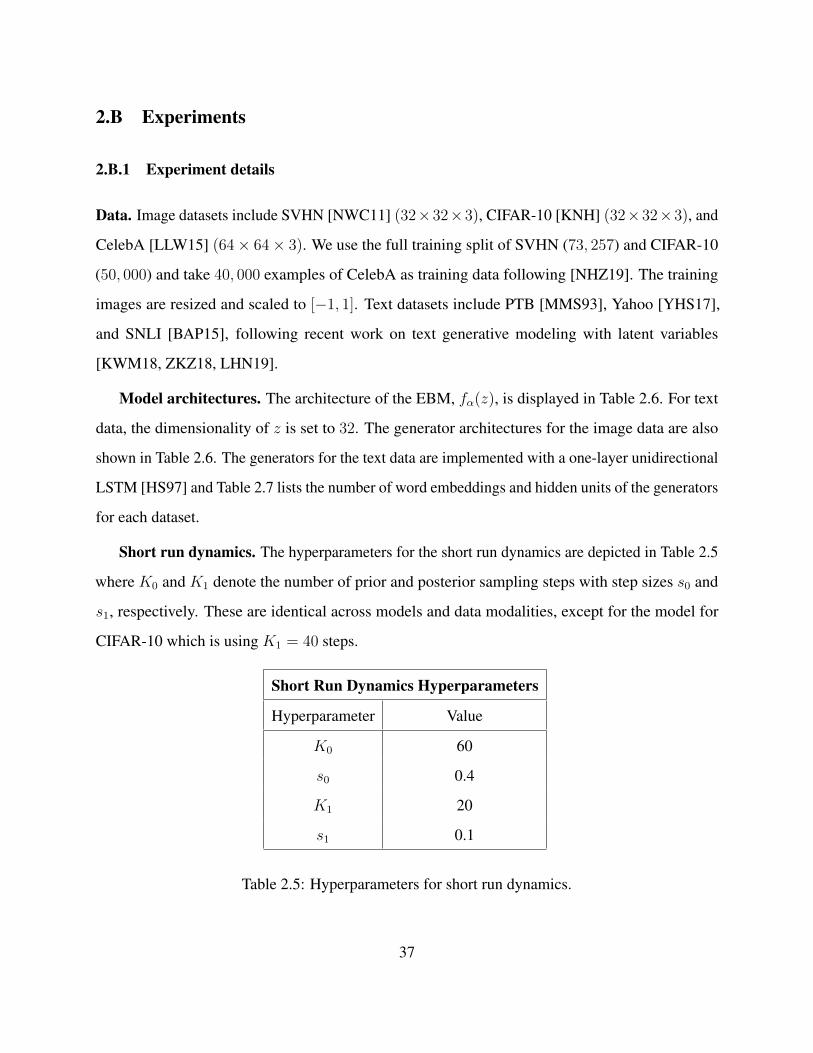
2.B Experiments

2.B.1 Experiment details

Data. Image datasets include SVHN [NWC11] (32×32×3), CIFAR-10 [KNH] (32×32×3), and

CelebA [LLW15] (64× 64× 3). We use the full training split of SVHN (73, 257) and CIFAR-10

(50, 000) and take 40, 000 examples of CelebA as training data following [NHZ19]. The training

images are resized and scaled to [−1, 1]. Text datasets include PTB [MMS93], Yahoo [YHS17],

and SNLI [BAP15], following recent work on text generative modeling with latent variables

[KWM18, ZKZ18, LHN19].

Model architectures. The architecture of the EBM, fα(z), is displayed in Table 2.6. For text

data, the dimensionality of z is set to 32. The generator architectures for the image data are also

shown in Table 2.6. The generators for the text data are implemented with a one-layer unidirectional

LSTM [HS97] and Table 2.7 lists the number of word embeddings and hidden units of the generators

for each dataset.

Short run dynamics. The hyperparameters for the short run dynamics are depicted in Table 2.5

where K0 and K1 denote the number of prior and posterior sampling steps with step sizes s0 and

s1, respectively. These are identical across models and data modalities, except for the model for

CIFAR-10 which is using K1 = 40 steps.

Short Run Dynamics Hyperparameters

Hyperparameter Value

K0 60

s0 0.4

K1 20

s1 0.1

Table 2.5: Hyperparameters for short run dynamics.

37

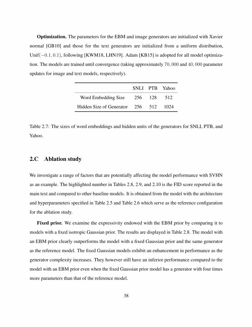
Optimization. The parameters for the EBM and image generators are initialized with Xavier

normal [GB10] and those for the text generators are initialized from a uniform distribution,

Unif(−0.1, 0.1), following [KWM18, LHN19]. Adam [KB15] is adopted for all model optimiza-

tion. The models are trained until convergence (taking approximately 70, 000 and 40, 000 parameter

updates for image and text models, respectively).

SNLI PTB Yahoo

Word Embedding Size 256 128 512

Hidden Size of Generator 256 512 1024

Table 2.7: The sizes of word embeddings and hidden units of the generators for SNLI, PTB, and

Yahoo.

2.C Ablation study

We investigate a range of factors that are potentially affecting the model performance with SVHN

as an example. The highlighted number in Tables 2.8, 2.9, and 2.10 is the FID score reported in the

main text and compared to other baseline models. It is obtained from the model with the architecture

and hyperparameters specified in Table 2.5 and Table 2.6 which serve as the reference configuration

for the ablation study.

Fixed prior. We examine the expressivity endowed with the EBM prior by comparing it to

models with a fixed isotropic Gaussian prior. The results are displayed in Table 2.8. The model with

an EBM prior clearly outperforms the model with a fixed Gaussian prior and the same generator

as the reference model. The fixed Gaussian models exhibit an enhancement in performance as the

generator complexity increases. They however still have an inferior performance compared to the

model with an EBM prior even when the fixed Gaussian prior model has a generator with four times

more parameters than that of the reference model.

38

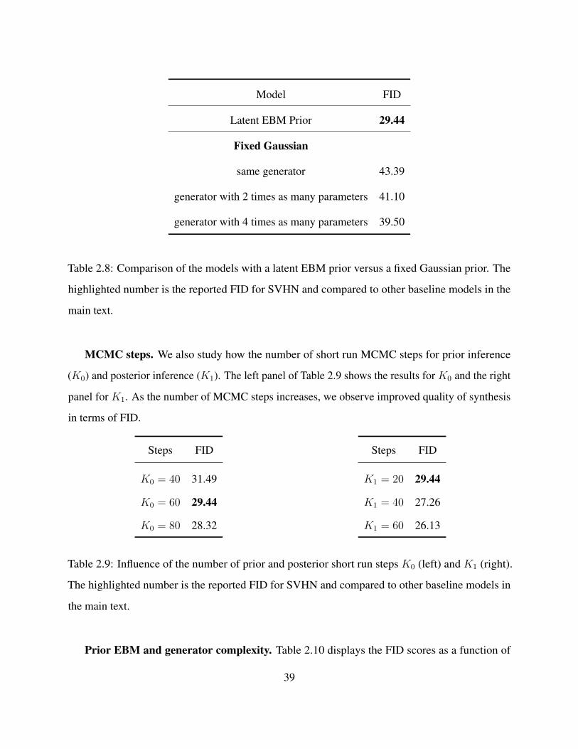
Model FID

Latent EBM Prior 29.44

Fixed Gaussian

same generator 43.39

generator with 2 times as many parameters 41.10

generator with 4 times as many parameters 39.50

Table 2.8: Comparison of the models with a latent EBM prior versus a fixed Gaussian prior. The

highlighted number is the reported FID for SVHN and compared to other baseline models in the

main text.

MCMC steps. We also study how the number of short run MCMC steps for prior inference

(K0) and posterior inference (K1). The left panel of Table 2.9 shows the results for K0 and the right

panel for K1. As the number of MCMC steps increases, we observe improved quality of synthesis

in terms of FID.

Steps FID

K0 = 40 31.49

K0 = 60 29.44

K0 = 80 28.32

Steps FID

K1 = 20 29.44

K1 = 40 27.26

K1 = 60 26.13

Table 2.9: Influence of the number of prior and posterior short run steps K0 (left) and K1 (right).

The highlighted number is the reported FID for SVHN and compared to other baseline models in

the main text.

Prior EBM and generator complexity. Table 2.10 displays the FID scores as a function of

39

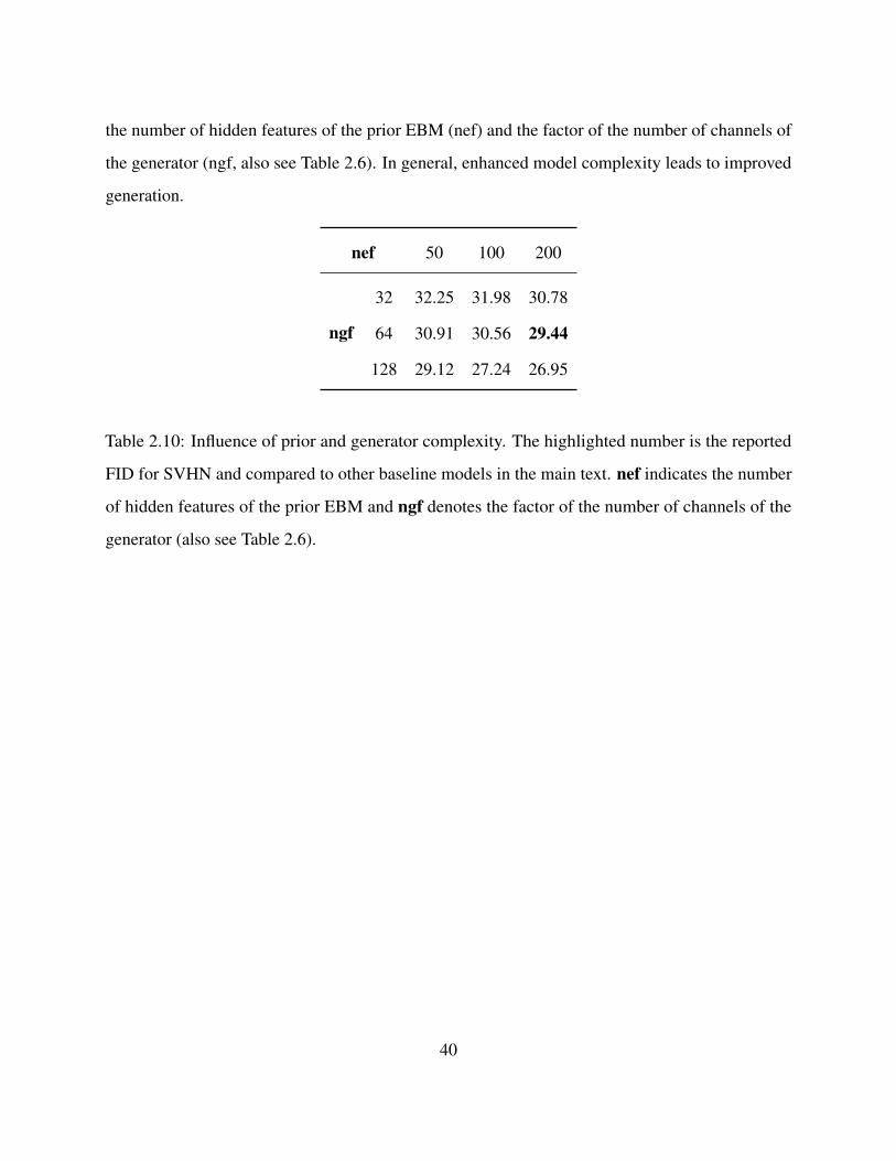
the number of hidden features of the prior EBM (nef) and the factor of the number of channels of

the generator (ngf, also see Table 2.6). In general, enhanced model complexity leads to improved

generation.

nef 50 100 200

ngf

32 32.25 31.98 30.78

64 30.91 30.56 29.44

128 29.12 27.24 26.95

Table 2.10: Influence of prior and generator complexity. The highlighted number is the reported

FID for SVHN and compared to other baseline models in the main text. nef indicates the number

of hidden features of the prior EBM and ngf denotes the factor of the number of channels of the

generator (also see Table 2.6).

40

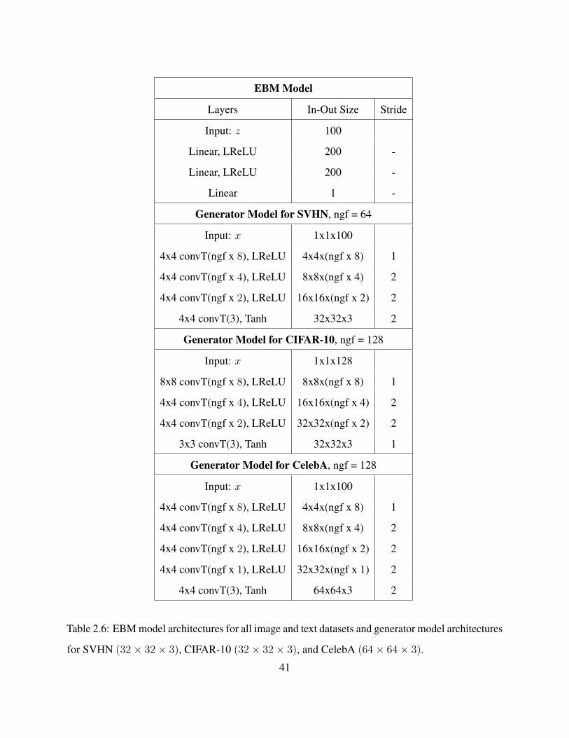
EBM Model

Layers In-Out Size Stride

Input: z 100

Linear, LReLU 200 -

Linear, LReLU 200 -

Linear 1 -

Generator Model for SVHN, ngf = 64

Input: x 1x1x100

4x4 convT(ngf x 8), LReLU 4x4x(ngf x 8) 1

4x4 convT(ngf x 4), LReLU 8x8x(ngf x 4) 2

4x4 convT(ngf x 2), LReLU 16x16x(ngf x 2) 2

4x4 convT(3), Tanh 32x32x3 2

Generator Model for CIFAR-10, ngf = 128

Input: x 1x1x128

8x8 convT(ngf x 8), LReLU 8x8x(ngf x 8) 1

4x4 convT(ngf x 4), LReLU 16x16x(ngf x 4) 2

4x4 convT(ngf x 2), LReLU 32x32x(ngf x 2) 2

3x3 convT(3), Tanh 32x32x3 1

Generator Model for CelebA, ngf = 128

Input: x 1x1x100

4x4 convT(ngf x 8), LReLU 4x4x(ngf x 8) 1

4x4 convT(ngf x 4), LReLU 8x8x(ngf x 4) 2

4x4 convT(ngf x 2), LReLU 16x16x(ngf x 2) 2

4x4 convT(ngf x 1), LReLU 32x32x(ngf x 1) 2

4x4 convT(3), Tanh 64x64x3 2

Table 2.6: EBM model architectures for all image and text datasets and generator model architectures

for SVHN (32× 32× 3), CIFAR-10 (32× 32× 3), and CelebA (64× 64× 3).

41

CHAPTER 3

Model Molecules with Latent Space Energy-Based Model

3.1 Introduction

In Chapter 2, we propose to unify EBM and generator model by learning an EBM as the prior

of an generator, yielding an expressive and efficient model, latent space EBM, and propose a

principled learning method. We have verified their effectiveness on natural images and text. In this

Chapter, we apply latent space EBM to a challenging domain, molecule modeling. We leverage the

expressiveness of latent space EBM to train a model that automatically learn complicated chemical

rules implicitly from the data.

3.2 Motivation

Designing molecules with desired properties is of vital importance in applications such as drug

design and material science. Molecules are in the form of graphs. It is hence challenging to search

for desirable ones in the molecule space. Recently, deep generative models have been applied to

molecule modeling [GWD18, KPH17, SK18, SXZ20, PBM20]. Most methods adopt Variational

Autoencoder (VAE) model [KW14]. It embeds molecules into a continuous latent space, allowing

for more efficient optimization, and then decodes the latent vector to a molecule, enabling new

molecule generation.

In molecule modeling, two types of representations are widely used. One is simplified molecular

input line entry systems (SMILES) [Wei88] with which a molecule graph is linearized into a string

42

consisting of characters that represent atoms and bonds. With this representation, an autoregressive

model can be utilized to capture the chemical rules among atoms and bonds. The same model is

widely used and called language model (LM) in natural language processing. Following [PBM20],

we call models adopting this representation as LM-based models. Another representation works

directly with the graph where nodes and edges represent atoms and bonds respectively. Graph allows

for explicitly encoding and directly enforcing chemical laws. To guarantee validity of generated

molecules, many graph-based models [LAB18, SAJ19, SXZ20] sequentially generate atoms (nodes)

and bonds (edges), continuously check if the generated elements satisfy valency rules. Graph-based

models are however more complicated and less efficient to train and sample from, compared to

LM-based models.

Despite the simplicity and efficiency of LM-based models, they often produce invalid samples

and duplicates. The recent work of [PBM20] proposed FragmentVAE and argued that LM-based

models can produce samples with perfect validity and uniqueness. Fragments are small-weight

and chemically sound compounds, and FragmentVAE uses fragments instead of atoms as basic

elements in molecule generation. To enhance uniqueness, FragmentVAE replaces infrequent

fragments in generated molecules by new fragments that are uniformly sampled from a pool of

infrequent fragments. These techniques make the SMILES-fragment-based model competitive with

the state-of-the-art graph-based models.

Instead of redesigning molecule representation or resorting to more complicated graph models,

we argue that an expressive model is sufficient to capture the complicated chemical rules implicitly

and generate valid and unique molecules, even with the character-level SMILES representation

instead of fragment-level representation. Previous VAE-based methods rely on a generator network

to map a prior distribution to be close to the data distribution and assume the prior to be a simple

isotropic Gaussian distribution. Although a neural network generator is highly expressive, the

assumption on the prior may cause ineffective learning of the model, which might explain why

previous methods fail to generate valid and unique molecules without explicitly enforcing chemical

rules. In this Chapter, we propose to learn a latent space energy-based prior model in addition to

43

the generator network from observed molecules. Specifically, the prior model is an energy-based

correction of the isotropic Gaussian distribution and the correction is learned from empirical data.

Such a prior model improves the expressivity of the generator model. Our experiments demonstrate

that our method is able to generate valid and unique samples, with the performance on par with the

state-of-the-art models. Interestingly, we observe that the generated samples show structural and

chemical properties (e.g., solubility, drug-likeness) that closely resemble the ground truth molecules.

3.3 Methods

3.3.1 Model

Let x ∈ RD be an observed molecule such as represented in SMILES strings. Let z ∈ Rd be the

latent variables, where D ≫ d. Consider the following model,

z ∼ pα(z), x ∼ pβ(x|z), (3.1)

where pα(z) is the prior model with parameters α, pβ(x|z) is the top-down generative model with

parameters β. In VAE, the prior is simply assumed to be an isotropic Gaussian distribution. In our

model, pα(z) is formulated as an energy-based model or a Gibbs distribution,

pα(z) =1

Z(α)exp(fα(z))p0(z). (3.2)

where p0(z) is a reference distribution, assumed to be isotropic Gaussian as in VAE. fα(z) is

the negative energy and is parameterized by a small multi-layer perceptron with parameters α.

Z(α) =∫exp(fα(z))p0(z)dz = Ep0 [exp(fα(z))] is the normalizing constant or partition function.

The generative model, pβ(x|z), is a conditional autoregressive model,

pβ(x|z) =T∏t=1

pβ(x(t)|x(1), ..., x(t−1), z) (3.3)

which is parameterized by a simple recurrent network with parameters β and x(t) indicates a one-hot

encoded SMILES string.

44

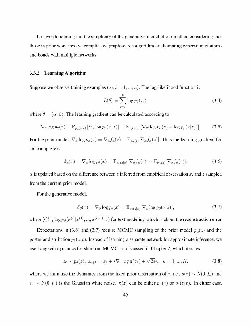
It is worth pointing out the simplicity of the generative model of our method considering that

those in prior work involve complicated graph search algorithm or alternating generation of atoms

and bonds with multiple networks.

3.3.2 Learning Algorithm

Suppose we observe training examples (xi, i = 1, ..., n). The log-likelihood function is

L(θ) =n∑i=1

log pθ(xi). (3.4)

where θ = (α, β). The learning gradient can be calculated according to

∇θ log pθ(x) = Epθ(z|x) [∇θ log pθ(x, z)] = Epθ(z|x) [∇θ(log pα(z) + log pβ(x|z))] . (3.5)

For the prior model, ∇α log pα(z) = ∇αfα(z) − Epα(z)[∇αfα(z)]. Thus the learning gradient for

an example x is

δα(x) = ∇α log pθ(x) = Epθ(z|x)[∇αfα(z)]− Epα(z)[∇αfα(z)]. (3.6)

α is updated based on the difference between z inferred from empirical observation x, and z sampled

from the current prior model.

For the generative model,

δβ(x) = ∇β log pθ(x) = Epθ(z|x)[∇β log pβ(x|z)], (3.7)

where∑T

t=1 log pβ(x(t)|x(1), ..., x(t−1), z) for text modeling which is about the reconstruction error.

Expectations in (3.6) and (3.7) require MCMC sampling of the prior model pα(z) and the

posterior distribution pθ(z|x). Instead of learning a separate network for approximate inference, we

use Langevin dynamics for short run MCMC, as discussed in Chapter 2, which iterates:

z0 ∼ p0(z), zk+1 = zk + s∇z log π(zk) +√2sϵk, k = 1, ..., K. (3.8)

where we initialize the dynamics from the fixed prior distribution of z, i.e., p(z) ∼ N(0, Id) and

ϵk ∼ N(0, Id) is the Gaussian white noise. π(z) can be either pα(z) or pθ(z|x). In either case,

45

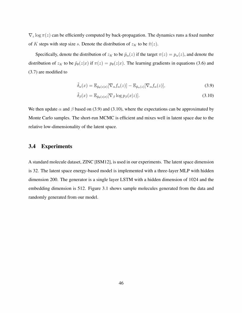
∇z log π(z) can be efficiently computed by back-propagation. The dynamics runs a fixed number

of K steps with step size s. Denote the distribution of zK to be π(z).

Specifically, denote the distribution of zK to be pα(z) if the target π(z) = pα(z), and denote the

distribution of zK to be pθ(z|x) if π(z) = pθ(z|x). The learning gradients in equations (3.6) and

(3.7) are modified to

δα(x) = Epθ(z|x)[∇αfα(z)]− Epα(z)[∇αfα(z)], (3.9)

δβ(x) = Epθ(z|x)[∇β log pβ(x|z)]. (3.10)

We then update α and β based on (3.9) and (3.10), where the expectations can be approximated by

Monte Carlo samples. The short-run MCMC is efficient and mixes well in latent space due to the

relative low-dimensionality of the latent space.

3.4 Experiments

A standard molecule dataset, ZINC [ISM12], is used in our experiments. The latent space dimension

is 32. The latent space energy-based model is implemented with a three-layer MLP with hidden

dimension 200. The generator is a single layer LSTM with a hidden dimension of 1024 and the

embedding dimension is 512. Figure 3.1 shows sample molecules generated from the data and

randomly generated from our model.

46

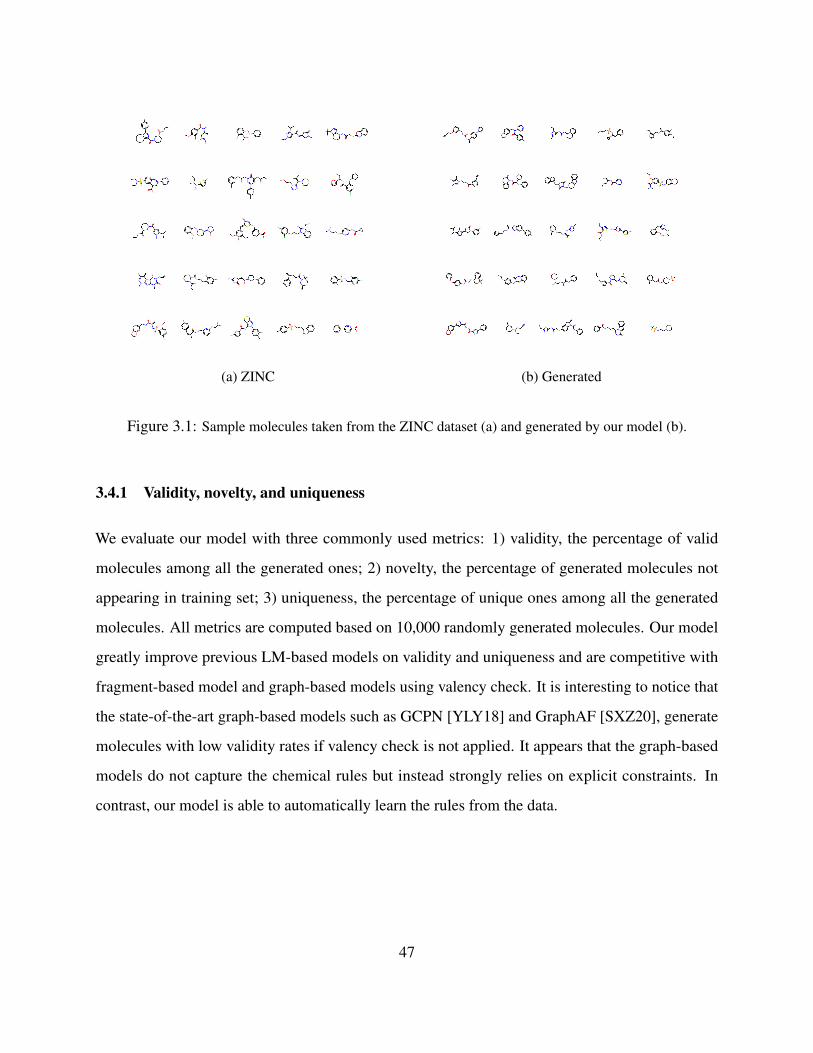
(a) ZINC (b) Generated

Figure 3.1: Sample molecules taken from the ZINC dataset (a) and generated by our model (b).

3.4.1 Validity, novelty, and uniqueness

We evaluate our model with three commonly used metrics: 1) validity, the percentage of valid

molecules among all the generated ones; 2) novelty, the percentage of generated molecules not

appearing in training set; 3) uniqueness, the percentage of unique ones among all the generated

molecules. All metrics are computed based on 10,000 randomly generated molecules. Our model

greatly improve previous LM-based models on validity and uniqueness and are competitive with

fragment-based model and graph-based models using valency check. It is interesting to notice that

the state-of-the-art graph-based models such as GCPN [YLY18] and GraphAF [SXZ20], generate

molecules with low validity rates if valency check is not applied. It appears that the graph-based

models do not capture the chemical rules but instead strongly relies on explicit constraints. In

contrast, our model is able to automatically learn the rules from the data.

47

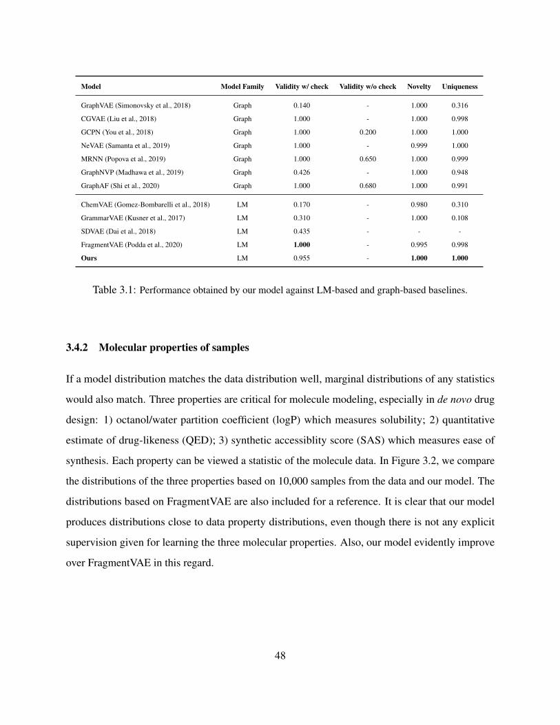
Model Model Family Validity w/ check Validity w/o check Novelty Uniqueness

GraphVAE (Simonovsky et al., 2018) Graph 0.140 - 1.000 0.316

CGVAE (Liu et al., 2018) Graph 1.000 - 1.000 0.998

GCPN (You et al., 2018) Graph 1.000 0.200 1.000 1.000

NeVAE (Samanta et al., 2019) Graph 1.000 - 0.999 1.000

MRNN (Popova et al., 2019) Graph 1.000 0.650 1.000 0.999

GraphNVP (Madhawa et al., 2019) Graph 0.426 - 1.000 0.948

GraphAF (Shi et al., 2020) Graph 1.000 0.680 1.000 0.991

ChemVAE (Gomez-Bombarelli et al., 2018) LM 0.170 - 0.980 0.310

GrammarVAE (Kusner et al., 2017) LM 0.310 - 1.000 0.108

SDVAE (Dai et al., 2018) LM 0.435 - - -

FragmentVAE (Podda et al., 2020) LM 1.000 - 0.995 0.998

Ours LM 0.955 - 1.000 1.000

Table 3.1: Performance obtained by our model against LM-based and graph-based baselines.

3.4.2 Molecular properties of samples

If a model distribution matches the data distribution well, marginal distributions of any statistics

would also match. Three properties are critical for molecule modeling, especially in de novo drug

design: 1) octanol/water partition coefficient (logP) which measures solubility; 2) quantitative

estimate of drug-likeness (QED); 3) synthetic accessiblity score (SAS) which measures ease of

synthesis. Each property can be viewed a statistic of the molecule data. In Figure 3.2, we compare

the distributions of the three properties based on 10,000 samples from the data and our model. The

distributions based on FragmentVAE are also included for a reference. It is clear that our model

produces distributions close to data property distributions, even though there is not any explicit

supervision given for learning the three molecular properties. Also, our model evidently improve

over FragmentVAE in this regard.

48

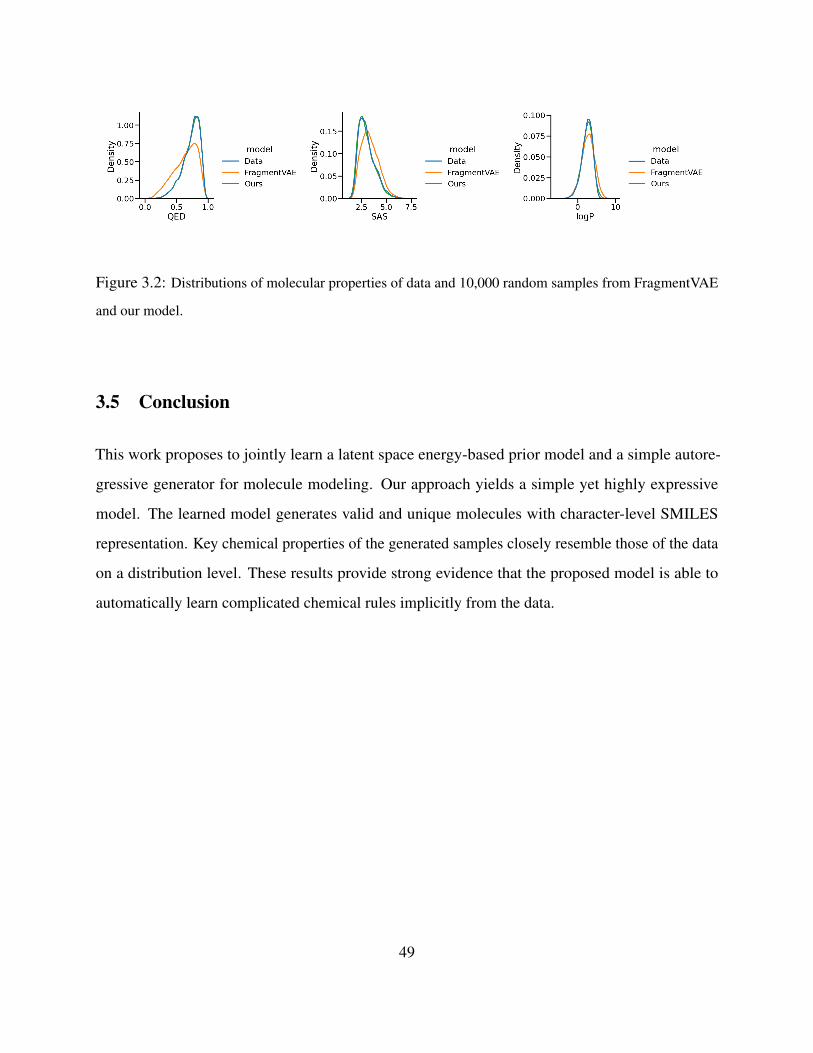
Figure 3.2: Distributions of molecular properties of data and 10,000 random samples from FragmentVAE

and our model.

3.5 Conclusion

This work proposes to jointly learn a latent space energy-based prior model and a simple autore-

gressive generator for molecule modeling. Our approach yields a simple yet highly expressive

model. The learned model generates valid and unique molecules with character-level SMILES

representation. Key chemical properties of the generated samples closely resemble those of the data

on a distribution level. These results provide strong evidence that the proposed model is able to

automatically learn complicated chemical rules implicitly from the data.

49

CHAPTER 4

Trajectory Prediction with Latent Belief Energy-Based Model

4.1 Introduction

In Chapter 2 and Chapter 3, we propose latent space EBM and leverage its expressivity to model

complex patterns including images, text, and molecule graphs. An alternative and interesting view

of an EBM is that it is a cost function and can be learned from expert demonstrations. Optimizing

over the cost function yields policy close to experts’ policy. This perspective connects our model

to inverse reinforcement learning. In this chapter, we study this aspect of latent space EBM.

In particular, the cost function or EBM is learned in the latent space of an generator, and an

inference network is learned jointly. Optimizing the learned cost function in the latent space can be

achieved with MCMC sampling such as Langevin dynamics, by exploiting the continuous nature

and smoothness of the latent space. The sampled vector can be mapped to the observed policy space

with the generator, while the inference network can map experts’ policy to the latent space, with

which the cost function is learned.

4.2 Motivation

Forecasting the future trajectories of pedestrians is critical for autonomous moving platforms

like self-driving cars or social robots with which humans are interacting. It has recently attracted

interest from many researchers [GJF18, ZXM19, LCV17, SKS19, BHF19, DT20, LJH20, MGA20].

See [RPH20] for an overview. Trajectory forecast is a challenging problem since human future

trajectories depend on a multitude of factors such as past movement history, goals, behavior of

50

surrounding pedestrians. Also, future paths are inherently multimodal. Given the past trajectories,

there are multiple possible future paths. We propose a latent belief energy-based model (LB-EBM)

which captures pedestrian behavior patterns and subtle social interaction norms in the latent space

and make multimodal trajectory predictions. LB-EBM is learned from expert demonstrations (i.e.,

human trajectories) following the principle of inverse reinforcement learning (IRL) [NR00, FCA16,

FLA16, HTA17].

Traditional IRL approaches [NR00] first learn a cost function from expert demonstrations in an

outer loop and then use reinforcement learning to extract the policy from the learned cost function

in an inner loop. These approaches are often highly computationally expensive. We learn an

energy-based model (EBM) as the cost function in a low dimensional latent space and map the

EBM distribution to actions with a policy generator. Similar to traditional IRL, we learn a cost

function but our cost function is defined in a low dimensional space so that our cost function is

easier to model and learn.

An EBM [XLZ16, NHZ19, PHN20] in the form of Boltzmann or Gibbs distribution maps a

latent vector to its probability. It has no restrictions in its form and can be instantiated by any

function approximators such as neural networks. Thus, this model is highly expressive and learning

from human trajectories allows it to capture the multimodality of the trajectory distribution. Our

proposed LB-EBM is defined in a latent space. An encoder is jointly learned to project human

trajectories into the latent space and hence provides expert demonstrations to the latent cost function.

Furthermore, this cost function accounts for trajectory history and motion behavior of surround-

ing pedestrians. Thus sampling from or optimizing the cost function yields a latent belief, regarding

future trajectory, which considers the centric agent’s behavior pattern and social context surrounding

this agent. A future trajectory is then forecasted in two steps or on two time scales. We first use the

social-aware latent belief vector to make a rough plan for future path. It is intuitive that human do

not plan every single future step in advance but we often have a rough idea about how to navigate

through our future path, which is based on one’s belief after observing other agents’ motion. The

belief is inherently related to the agent’s behavior pattern. This forms the intuitive motivation of our

51

modeling approach. Conditioned on the plan, the trajectory is then predicted with the assistance of

individual motion history and social cues. Several recent works take two steps to make trajectory

forecast. They either first estimate the final goal [MGA20] or make a plan on a coarse grid map

[LJM20]. We take a similar approach. The plan in our approach is defined to be positions of some

well-separated steps in the future trajectory, which can be easily extracted from the data.

The proposed LB-EBM and other modules are learned end-to-end. We test our model on the

Stanford Drone (SDD) trajectory prediction benchmark and the ETH-UCY benchmark and improves

the prior state-of-the-art performance by 10.9% on SDD and 27.6% on ETH-UCY.

Our work has the following contributions.

• We propose a latent belief energy-based model (LB-EBM), following the principle of IRL,

which naturally captures the multimodal human trajectory distribution.

• Our approach predicts multimodal and social compliant future trajectories.

• Our model achieves the state-of-the-art on widely-used human trajectory forecasting bench-

marks.

4.3 Related work

Agents’ motions depend on their histories, goals, social interactions with other agents, constraints

from the scene context, and are inherently stochastic and multimodal. Conventional methods of

human trajectory forecasting model contextual constraints by hand-crafted features or cost functions

[DRT18, HM95, YBO11]. With the recent success of deep networks, RNN-based approaches have

become prevalent. These works propose to model interactions among multiple agents by applying

aggregation functions on their RNN hidden states [AGR16, GJF18, HST18], running convolutional

layers on agents’ spatial feature maps [DT18a, DMD20, ZXM19, WCM20], or leveraging attention

mechanisms or relational reasoning on constructed graphs of agents [LYT20, SKS19, SLV17,

52

ZOZ19, VMO18]. Some recent studies are, however, rethinking the use of RNN and social

information in modeling temporal dependencies and borrowing the idea of transformers into the

area [GHC20]. We apply these social interaction modeling approaches with a few modifications in

our work.

Modeling Goals. Recent progress has suggested that directly modeling goals could significantly

decrease the error for trajectory forecasting. [RMK19] introduces a prediction method conditioning

on agent goals. [MGA20] proposes to first predict the goal based on agents’ individual histories

and then to forecast future trajectories conditioning on the predicted goal. [LJM20] introduces a

two-step planning scheme, first in a coarse grid then in a finer one, which can be viewed as directly

modeling goals and sub-goals. We follow the general scheme of two-step prediction. The plan in

our approach is defined to be positions of some well-separated steps in the future trajectory, which

can be easily extracted from the data.

Multimodality. Most recent prediction works have emphasized more on modeling the multi-

modality nature of human motions. [BHL16, DT18b] directly predict multiple possible maneuvers

and generate corresponding future trajectories given each maneuver. [LCV17, IP19] use Varia-

tional Auto-Encoders [DM14] and [GJF18, LCV17, SKS19, ZXM19] use Generative Adversarial

Networks [GPM14a, MO14] to learn distributions. Many works [LJM20, PGB20, RKV18, TS19]

also focus on developing new datasets, proposing different formulations, utilizing latent variable

inference, and exploring new loss functions to account for multimodality. Our work adopts the

likelihood-based learning framework with variational inference. We propose a novel way to model

the multimodality of human trajectories, by projecting them into a latent space with variational

inference and leveraging the strength of latent space energy-based model.

Value Function. Human behaviors are observed as actions, e.g. trajectories, but the actions

are actually guided by hidden value functions, revealing human preference and cost over different

actions. Some previous works explicitly or implicitly model these types of cost functions as

intermediate steps for sampling possible futures. These works generally follow the reinforcement

learning formulation of value functionsQ. [NY11] directly uses Q-Learning to learn value functions.

53

[XZB19, KMW17] formulate trajectory planning and prediction problems as inverse optimal control

and GAIL (generative adversarial imitation learning) problems. [MHL17] models social interaction

by game theory and attempt to find the hidden human value by fictitious play. P2TIRL [DT20] is

learned by a maximum entropy inverse reinforcement learning (IRL). Our work also follows the

basic principle of inverse reinforcement learning to learn human cost functions explicitly in a latent

space.

Energy-Based Models. The energy function in the EBM [ZWM98b, XLZ16, NHZ19, DM19,

HNZ20a] can be viewed as an objective function, a cost function, or a critic [SB18]. It captures

regularities, rules or constrains. It is easy to specify, although optimizing or sampling the energy

function requires iterative computation such as MCMC. Our earlier works, as discussed in Chapter

2 and Chapter 3 in this dissertation, proposed to learn EBM in a low dimensional latent space,

which makes optimizing or sampling the energy function much more efficient and convenient. This

Chapter follows this approach.

4.4 Model and learning

4.4.1 Problem definition

Let xti ∈ R2 denote the position of a person i at time t in a scene where there are n people in

total. The history trajectory of the person i is xxxi = {xti, t = 1, ..., tpast} andXXX = {xxxi, i = 1, ..., n}

collects past trajectories of all people in a scene. Similarly, the future trajectory of this person at

time t is denoted as yti . yyyi = {yti , t = tpast + 1, ..., tpred} and YYY = {yyyi, i = 1, ..., n} indicate the

future trajectory of the person i and all future trajectories, respectively. The goal is to jointly predict

the future trajectories of all the agents in the scene or to learn the probabilistic distribution, p(YYY |XXX).

Directly modeling p(YYY |XXX) is essentially supervised learning or behavior cloning which often

fails to capture the multimodality. Instead, we introduce two auxiliary variables. The first is zzzi

which represents the latent belief of the agent i after observing the trajectory history of his or her

54

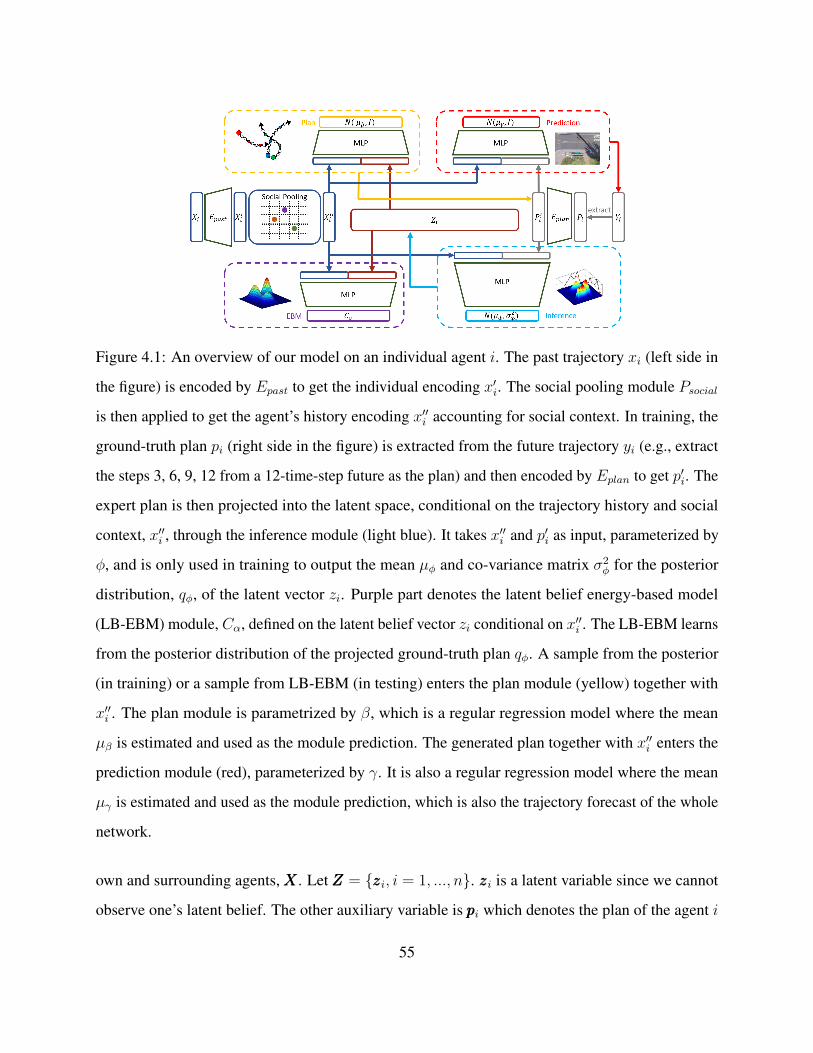
Figure 4.1: An overview of our model on an individual agent i. The past trajectory xi (left side in

the figure) is encoded by Epast to get the individual encoding x′i. The social pooling module Psocial

is then applied to get the agent’s history encoding x′′i accounting for social context. In training, the

ground-truth plan pi (right side in the figure) is extracted from the future trajectory yi (e.g., extract

the steps 3, 6, 9, 12 from a 12-time-step future as the plan) and then encoded by Eplan to get p′i. The

expert plan is then projected into the latent space, conditional on the trajectory history and social

context, x′′i , through the inference module (light blue). It takes x′′i and p′i as input, parameterized by

ϕ, and is only used in training to output the mean µϕ and co-variance matrix σ2ϕ for the posterior

distribution, qϕ, of the latent vector zi. Purple part denotes the latent belief energy-based model

(LB-EBM) module, Cα, defined on the latent belief vector zi conditional on x′′i . The LB-EBM learns

from the posterior distribution of the projected ground-truth plan qϕ. A sample from the posterior

(in training) or a sample from LB-EBM (in testing) enters the plan module (yellow) together with

x′′i . The plan module is parametrized by β, which is a regular regression model where the mean

µβ is estimated and used as the module prediction. The generated plan together with x′′i enters the

prediction module (red), parameterized by γ. It is also a regular regression model where the mean

µγ is estimated and used as the module prediction, which is also the trajectory forecast of the whole

network.

own and surrounding agents,XXX . Let ZZZ = {zzzi, i = 1, ..., n}. zzzi is a latent variable since we cannot

observe one’s latent belief. The other auxiliary variable is pppi which denotes the plan of the agent i

55

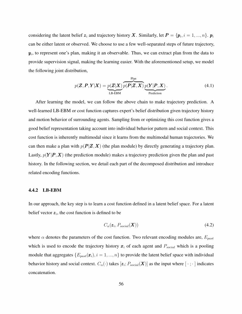
considering the latent belief zzzi and trajectory history XXX . Similarly, let PPP = {pppi, i = 1, ..., n}. pppi

can be either latent or observed. We choose to use a few well-separated steps of future trajectory,

yyyi, to represent one’s plan, making it an observable. Thus, we can extract plan from the data to

provide supervision signal, making the learning easier. With the aforementioned setup, we model

the following joint distribution,

p(ZZZ,PPP ,YYY |XXX) = p(ZZZ|XXX)︸ ︷︷ ︸LB-EBM

Plan︷ ︸︸ ︷p(PPP |ZZZ,XXX) p(YYY |PPP ,XXX)︸ ︷︷ ︸

Prediction

. (4.1)

After learning the model, we can follow the above chain to make trajectory prediction. A

well-learned LB-EBM or cost function captures expert’s belief distribution given trajectory history

and motion behavior of surrounding agents. Sampling from or optimizing this cost function gives a

good belief representation taking account into individual behavior pattern and social context. This

cost function is inherently multimodal since it learns from the multimodal human trajectories. We

can then make a plan with p(PPP |ZZZ,XXX) (the plan module) by directly generating a trajectory plan.

Lastly, p(YYY |PPP ,XXX) (the prediction module) makes a trajectory prediction given the plan and past

history. In the following section, we detail each part of the decomposed distribution and introduce

related encoding functions.

4.4.2 LB-EBM

In our approach, the key step is to learn a cost function defined in a latent belief space. For a latent

belief vector zzzi, the cost function is defined to be

Cα(zzzi, Psocial(XXX)) (4.2)

where α denotes the parameters of the cost function. Two relevant encoding modules are, Epast

which is used to encode the trajectory history xxxi of each agent and Psocial which is a pooling

module that aggregates {Epast(xxxi), i = 1, ..., n} to provide the latent belief space with individual

behavior history and social context. Cα(·) takes [zzzi;Psocial(XXX)] as the input where [ · ; · ] indicates

concatenation.

56

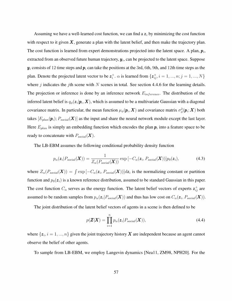
Assuming we have a well-learned cost function, we can find a zzzi by minimizing the cost function

with respect to it givenXXX , generate a plan with the latent belief, and then make the trajectory plan.

The cost function is learned from expert demonstrations projected into the latent space. A plan, pppi,

extracted from an observed future human trajectory, yyyi, can be projected to the latent space. Suppose

yyyi consists of 12 time steps and pppi can take the positions at the 3rd, 6th, 9th, and 12th time steps as the

plan. Denote the projected latent vector to be zzz+i . α is learned from {zzz+ij, i = 1, ..., n; j = 1, ..., N}

where j indicates the jth scene with N scenes in total. See section 4.4.6 for the learning details.

The projection or inference is done by an inference network Einference. The distribution of the

inferred latent belief is qϕ(zzzi|pppi,XXX), which is assumed to be a multivariate Gaussian with a diagonal

covariance matrix. In particular, the mean function µϕ(pppi,XXX) and covariance matrix σ2ϕ(pppi;XXX) both

takes [Eplan(pppi);Psocial(XXX)] as the input and share the neural network module except the last layer.

Here Eplan is simply an embedding function which encodes the plan pppi into a feature space to be

ready to concatenate with Psocial(XXX).

The LB-EBM assumes the following conditional probability density function

pα(zzzi|Psocial(XXX)) =1

Zα(Psocial(XXX))exp [−Cα(zzzi, Psocial(XXX))]p0(zzzi), (4.3)

where Zα(Psocial(XXX)) =∫exp [−Cα(zzzi, Psocial(XXX))]dzzzi is the normalizing constant or partition

function and p0(zzzi) is a known reference distribution, assumed to be standard Gaussian in this paper.

The cost function Cα serves as the energy function. The latent belief vectors of experts zzz+ij are

assumed to be random samples from pα(zzzi|Psocial(XXX)) and thus has low cost on Cα(zzzi, Psocial(XXX)).

The joint distribution of the latent belief vectors of agents in a scene is then defined to be

p(ZZZ|XXX) =n∏i=1

pα(zzzi|Psocial(XXX)), (4.4)

where {zzzi, i = 1, ..., n} given the joint trajectory historyXXX are independent because an agent cannot

observe the belief of other agents.

To sample from LB-EBM, we employ Langevin dynamics [Nea11, ZM98, NPH20]. For the

57

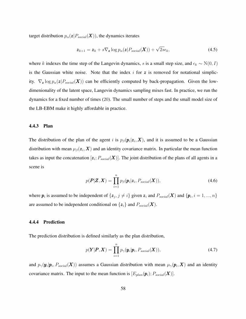
target distribution pα(zzz|Psocial(XXX)), the dynamics iterates

zzzk+1 = zzzk + s∇zzz log pα(zzz|Psocial(XXX)) +√2sϵk, (4.5)

where k indexes the time step of the Langevin dynamics, s is a small step size, and ϵk ∼ N(0, I)

is the Gaussian white noise. Note that the index i for zzz is removed for notational simplic-

ity. ∇zzz log pα(zzz|Psocial(XXX)) can be efficiently computed by back-propagation. Given the low-

dimenionality of the latent space, Langevin dynamics sampling mixes fast. In practice, we run the

dynamics for a fixed number of times (20). The small number of steps and the small model size of

the LB-EBM make it highly affordable in practice.

4.4.3 Plan

The distribution of the plan of the agent i is pβ(pppi|zzzi,XXX), and it is assumed to be a Gaussian

distribution with mean µβ(zzzi,XXX) and an identity covariance matrix. In particular the mean function

takes as input the concatenation [zzzi;Psocial(XXX)]. The joint distribution of the plans of all agents in a

scene is

p(PPP |ZZZ,XXX) =n∏i=1

pβ(pppi|zzzi, Psocial(XXX)), (4.6)

where pppi is assumed to be independent of {zzzj, j = i} given zzzi and Psocial(XXX) and {pppi, i = 1, ..., n}

are assumed to be independent conditional on {zzzi} and Psocial(XXX).

4.4.4 Prediction

The prediction distribution is defined similarly as the plan distribution,

p(YYY |PPP ,XXX) =n∏i=1

pγ(yyyi|pppi, Psocial(XXX)), (4.7)

and pγ(yyyi|pppi, Psocial(XXX)) assumes a Gaussian distribution with mean µγ(pppi,XXX) and an identity

covariance matrix. The input to the mean function is [Eplan(pppi);Psocial(XXX)].

58

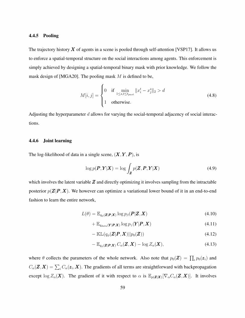
4.4.5 Pooling

The trajectory historyXXX of agents in a scene is pooled through self-attention [VSP17]. It allows us

to enforce a spatial-temporal structure on the social interactions among agents. This enforcement is

simply achieved by designing a spatial-temporal binary mask with prior knowledge. We follow the

mask design of [MGA20]. The pooling mask M is defined to be,

M [i, j] =

0 if min

1≤s,t≤tpast∥xti − xsj∥2 > d

1 otherwise.(4.8)

Adjusting the hyperparameter d allows for varying the social-temporal adjacency of social interac-

tions.

4.4.6 Joint learning

The log-likelihood of data in a single scene, (XXX,YYY ,PPP ), is

log p(PPP ,YYY |XXX) = log

∫ZZZ

p(ZZZ,PPP ,YYY |XXX) (4.9)

which involves the latent variableZZZ and directly optimizing it involves sampling from the intractable

posterior p(ZZZ|PPP ,XXX). We however can optimize a variational lower bound of it in an end-to-end

fashion to learn the entire network,

L(θ) = Eqϕ(ZZZ|PPP ,XXX) log pβ(PPP |ZZZ,XXX) (4.10)

+ Eqdata(YYY |PPP ,XXX) log pγ(YYY |PPP ,XXX) (4.11)

−KL(qϕ(ZZZ|PPP ,XXX)||p0(ZZZ)) (4.12)

− Eqϕ(ZZZ|PPP ,XXX)Cα(ZZZ,XXX)− logZα(XXX), (4.13)

where θ collects the parameters of the whole network. Also note that p0(ZZZ) =∏

i p0(zzzi) and

Cα(ZZZ,XXX) =∑

iCα(zzzi,XXX). The gradients of all terms are straightforward with backpropagation

except logZα(XXX). The gradient of it with respect to α is Ep(ZZZ|XXX)[∇αCα(ZZZ,XXX)]. It involves

59

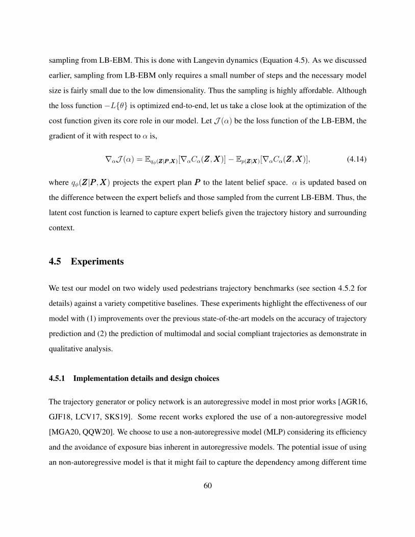
sampling from LB-EBM. This is done with Langevin dynamics (Equation 4.5). As we discussed

earlier, sampling from LB-EBM only requires a small number of steps and the necessary model

size is fairly small due to the low dimensionality. Thus the sampling is highly affordable. Although

the loss function −L{θ} is optimized end-to-end, let us take a close look at the optimization of the

cost function given its core role in our model. Let J (α) be the loss function of the LB-EBM, the

gradient of it with respect to α is,

∇αJ (α) = Eqϕ(ZZZ|PPP ,XXX)[∇αCα(ZZZ,XXX)]− Ep(ZZZ|XXX)[∇αCα(ZZZ,XXX)], (4.14)

where qϕ(ZZZ|PPP ,XXX) projects the expert plan PPP to the latent belief space. α is updated based on

the difference between the expert beliefs and those sampled from the current LB-EBM. Thus, the

latent cost function is learned to capture expert beliefs given the trajectory history and surrounding

context.

4.5 Experiments

We test our model on two widely used pedestrians trajectory benchmarks (see section 4.5.2 for

details) against a variety competitive baselines. These experiments highlight the effectiveness of our

model with (1) improvements over the previous state-of-the-art models on the accuracy of trajectory

prediction and (2) the prediction of multimodal and social compliant trajectories as demonstrate in

qualitative analysis.

4.5.1 Implementation details and design choices

The trajectory generator or policy network is an autoregressive model in most prior works [AGR16,

GJF18, LCV17, SKS19]. Some recent works explored the use of a non-autoregressive model

[MGA20, QQW20]. We choose to use a non-autoregressive model (MLP) considering its efficiency

and the avoidance of exposure bias inherent in autoregressive models. The potential issue of using

an non-autoregressive model is that it might fail to capture the dependency among different time

60

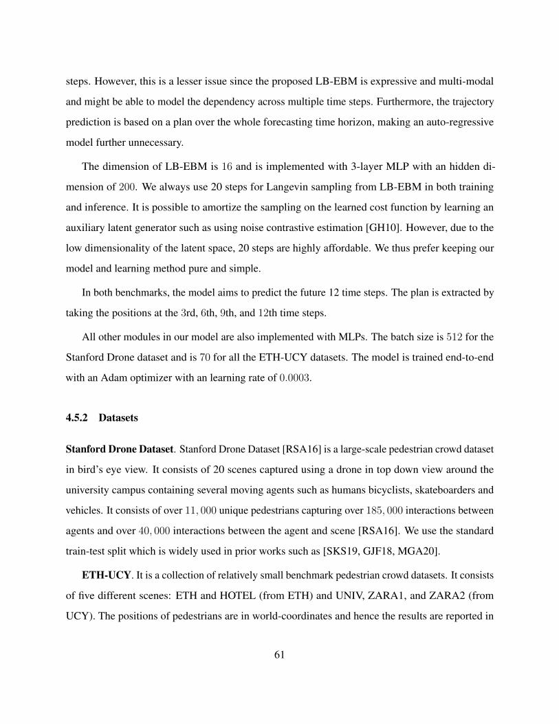
steps. However, this is a lesser issue since the proposed LB-EBM is expressive and multi-modal

and might be able to model the dependency across multiple time steps. Furthermore, the trajectory

prediction is based on a plan over the whole forecasting time horizon, making an auto-regressive

model further unnecessary.

The dimension of LB-EBM is 16 and is implemented with 3-layer MLP with an hidden di-

mension of 200. We always use 20 steps for Langevin sampling from LB-EBM in both training

and inference. It is possible to amortize the sampling on the learned cost function by learning an

auxiliary latent generator such as using noise contrastive estimation [GH10]. However, due to the

low dimensionality of the latent space, 20 steps are highly affordable. We thus prefer keeping our

model and learning method pure and simple.

In both benchmarks, the model aims to predict the future 12 time steps. The plan is extracted by

taking the positions at the 3rd, 6th, 9th, and 12th time steps.

All other modules in our model are also implemented with MLPs. The batch size is 512 for the

Stanford Drone dataset and is 70 for all the ETH-UCY datasets. The model is trained end-to-end

with an Adam optimizer with an learning rate of 0.0003.

4.5.2 Datasets

Stanford Drone Dataset. Stanford Drone Dataset [RSA16] is a large-scale pedestrian crowd dataset

in bird’s eye view. It consists of 20 scenes captured using a drone in top down view around the

university campus containing several moving agents such as humans bicyclists, skateboarders and

vehicles. It consists of over 11, 000 unique pedestrians capturing over 185, 000 interactions between

agents and over 40, 000 interactions between the agent and scene [RSA16]. We use the standard

train-test split which is widely used in prior works such as [SKS19, GJF18, MGA20].

ETH-UCY. It is a collection of relatively small benchmark pedestrian crowd datasets. It consists

of five different scenes: ETH and HOTEL (from ETH) and UNIV, ZARA1, and ZARA2 (from

UCY). The positions of pedestrians are in world-coordinates and hence the results are reported in

61

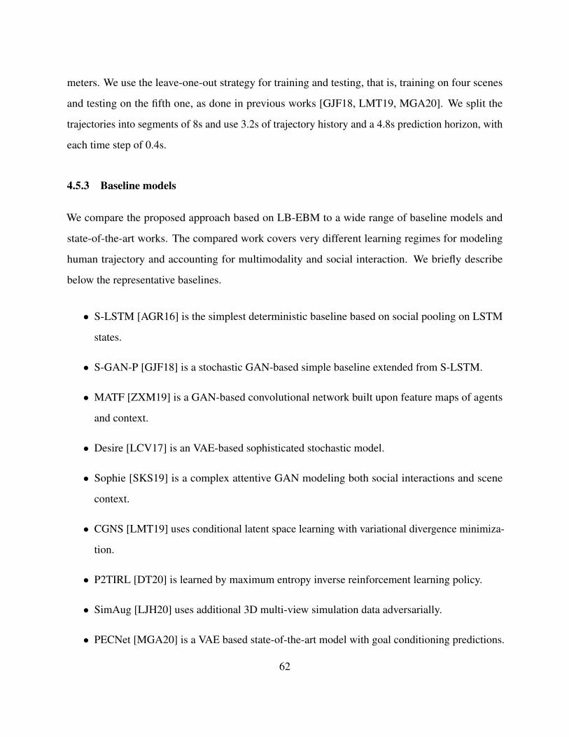
meters. We use the leave-one-out strategy for training and testing, that is, training on four scenes

and testing on the fifth one, as done in previous works [GJF18, LMT19, MGA20]. We split the

trajectories into segments of 8s and use 3.2s of trajectory history and a 4.8s prediction horizon, with

each time step of 0.4s.

4.5.3 Baseline models

We compare the proposed approach based on LB-EBM to a wide range of baseline models and

state-of-the-art works. The compared work covers very different learning regimes for modeling

human trajectory and accounting for multimodality and social interaction. We briefly describe

below the representative baselines.

• S-LSTM [AGR16] is the simplest deterministic baseline based on social pooling on LSTM

states.

• S-GAN-P [GJF18] is a stochastic GAN-based simple baseline extended from S-LSTM.

• MATF [ZXM19] is a GAN-based convolutional network built upon feature maps of agents

and context.

• Desire [LCV17] is an VAE-based sophisticated stochastic model.

• Sophie [SKS19] is a complex attentive GAN modeling both social interactions and scene

context.

• CGNS [LMT19] uses conditional latent space learning with variational divergence minimiza-

tion.

• P2TIRL [DT20] is learned by maximum entropy inverse reinforcement learning policy.

• SimAug [LJH20] uses additional 3D multi-view simulation data adversarially.

• PECNet [MGA20] is a VAE based state-of-the-art model with goal conditioning predictions.

62

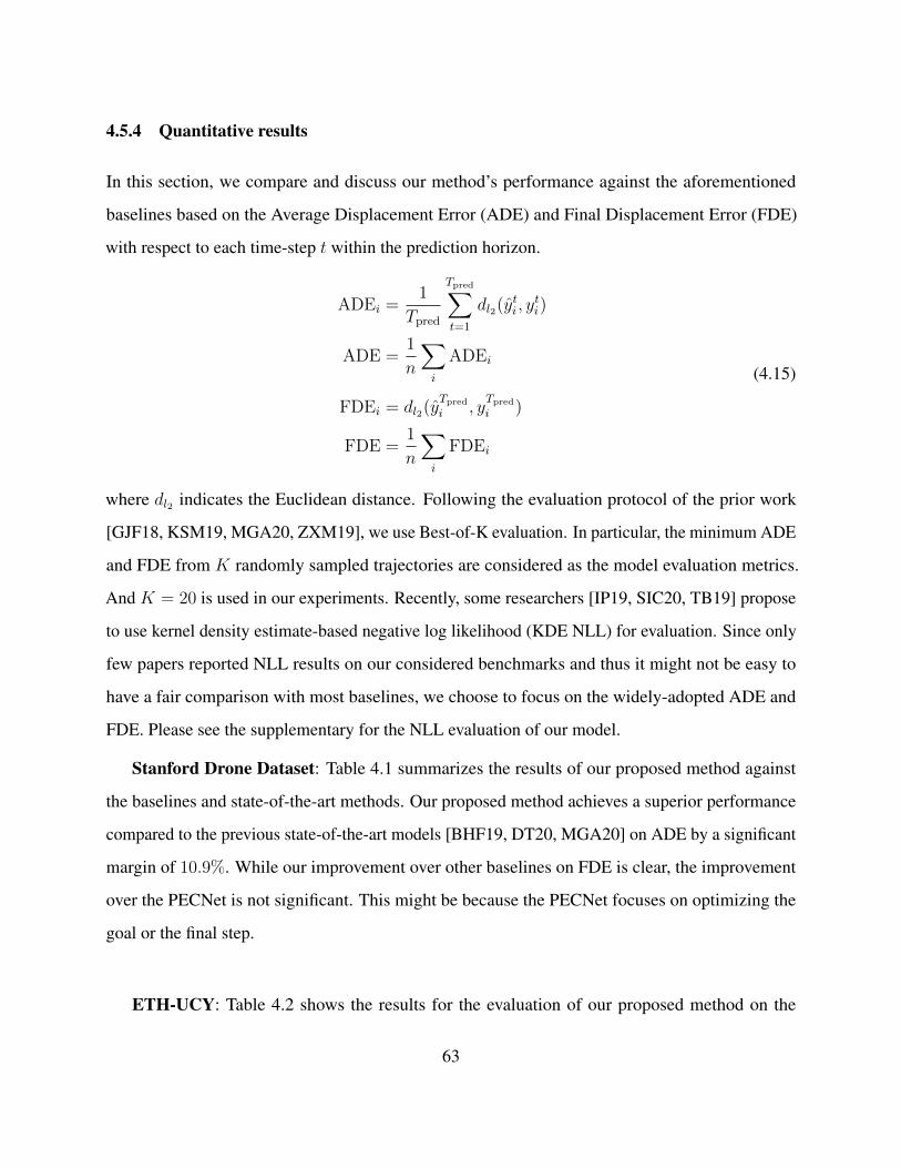
4.5.4 Quantitative results

In this section, we compare and discuss our method’s performance against the aforementioned

baselines based on the Average Displacement Error (ADE) and Final Displacement Error (FDE)

with respect to each time-step t within the prediction horizon.

ADEi =1

Tpred

Tpred∑t=1

dl2(yti , y

ti)

ADE =1

n

∑i

ADEi

FDEi = dl2(yTpredi , y

Tpredi )

FDE =1

n

∑i

FDEi

(4.15)

where dl2 indicates the Euclidean distance. Following the evaluation protocol of the prior work

[GJF18, KSM19, MGA20, ZXM19], we use Best-of-K evaluation. In particular, the minimum ADE

and FDE from K randomly sampled trajectories are considered as the model evaluation metrics.

And K = 20 is used in our experiments. Recently, some researchers [IP19, SIC20, TB19] propose

to use kernel density estimate-based negative log likelihood (KDE NLL) for evaluation. Since only

few papers reported NLL results on our considered benchmarks and thus it might not be easy to

have a fair comparison with most baselines, we choose to focus on the widely-adopted ADE and

FDE. Please see the supplementary for the NLL evaluation of our model.

Stanford Drone Dataset: Table 4.1 summarizes the results of our proposed method against

the baselines and state-of-the-art methods. Our proposed method achieves a superior performance

compared to the previous state-of-the-art models [BHF19, DT20, MGA20] on ADE by a significant

margin of 10.9%. While our improvement over other baselines on FDE is clear, the improvement

over the PECNet is not significant. This might be because the PECNet focuses on optimizing the

goal or the final step.

ETH-UCY: Table 4.2 shows the results for the evaluation of our proposed method on the

63

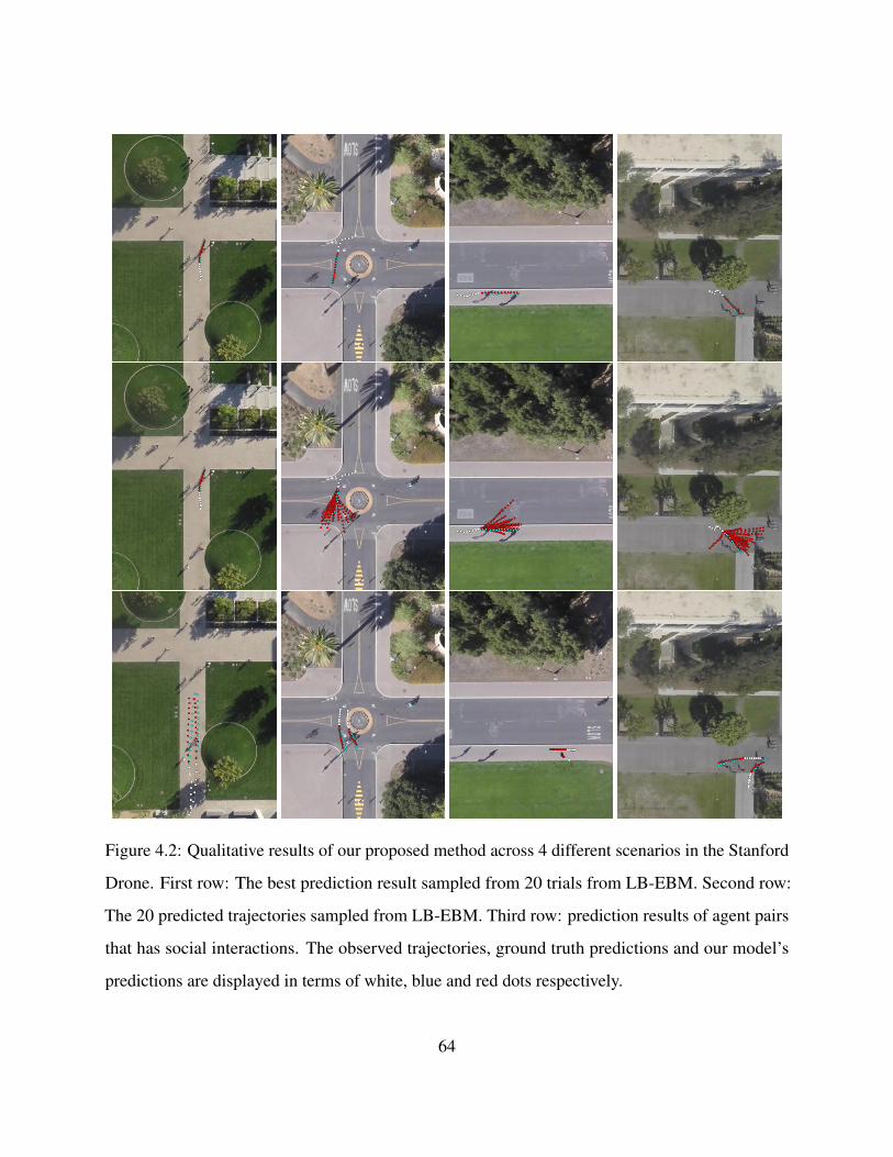
Figure 4.2: Qualitative results of our proposed method across 4 different scenarios in the Stanford

Drone. First row: The best prediction result sampled from 20 trials from LB-EBM. Second row:

The 20 predicted trajectories sampled from LB-EBM. Third row: prediction results of agent pairs

that has social interactions. The observed trajectories, ground truth predictions and our model’s

predictions are displayed in terms of white, blue and red dots respectively.

64

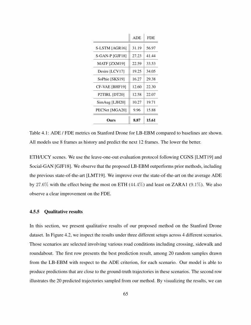
ADE FDE

S-LSTM [AGR16] 31.19 56.97

S-GAN-P [GJF18] 27.23 41.44

MATF [ZXM19] 22.59 33.53

Desire [LCV17] 19.25 34.05

SoPhie [SKS19] 16.27 29.38

CF-VAE [BHF19] 12.60 22.30

P2TIRL [DT20] 12.58 22.07

SimAug [LJH20] 10.27 19.71

PECNet [MGA20] 9.96 15.88

Ours 8.87 15.61

Table 4.1: ADE / FDE metrics on Stanford Drone for LB-EBM compared to baselines are shown.

All models use 8 frames as history and predict the next 12 frames. The lower the better.

ETH/UCY scenes. We use the leave-one-out evaluation protocol following CGNS [LMT19] and

Social-GAN [GJF18]. We observe that the proposed LB-EBM outperforms prior methods, including

the previous state-of-the-art [LMT19]. We improve over the state-of-the-art on the average ADE

by 27.6% with the effect being the most on ETH (44.4%) and least on ZARA1 (9.1%). We also

observe a clear improvement on the FDE.

4.5.5 Qualitative results

In this section, we present qualitative results of our proposed method on the Stanford Drone

dataset. In Figure 4.2, we inspect the results under three different setups across 4 different scenarios.

Those scenarios are selected involving various road conditions including crossing, sidewalk and

roundabout. The first row presents the best prediction result, among 20 random samples drawn

from the LB-EBM with respect to the ADE criterion, for each scenario. Our model is able to

produce predictions that are close to the ground-truth trajectories in these scenarios. The second row

illustrates the 20 predicted trajectories sampled from our method. By visualizing the results, we can

65

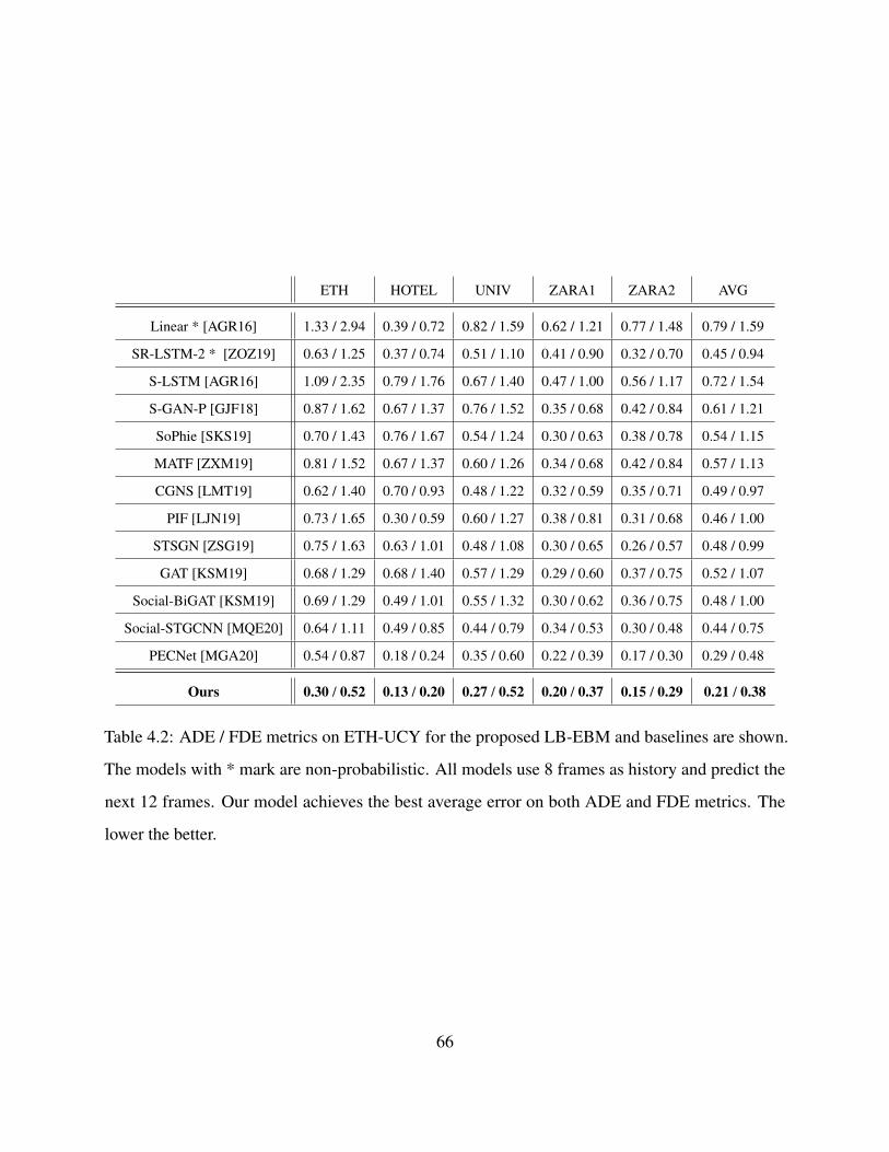
ETH HOTEL UNIV ZARA1 ZARA2 AVG

Linear * [AGR16] 1.33 / 2.94 0.39 / 0.72 0.82 / 1.59 0.62 / 1.21 0.77 / 1.48 0.79 / 1.59

SR-LSTM-2 * [ZOZ19] 0.63 / 1.25 0.37 / 0.74 0.51 / 1.10 0.41 / 0.90 0.32 / 0.70 0.45 / 0.94

S-LSTM [AGR16] 1.09 / 2.35 0.79 / 1.76 0.67 / 1.40 0.47 / 1.00 0.56 / 1.17 0.72 / 1.54

S-GAN-P [GJF18] 0.87 / 1.62 0.67 / 1.37 0.76 / 1.52 0.35 / 0.68 0.42 / 0.84 0.61 / 1.21

SoPhie [SKS19] 0.70 / 1.43 0.76 / 1.67 0.54 / 1.24 0.30 / 0.63 0.38 / 0.78 0.54 / 1.15

MATF [ZXM19] 0.81 / 1.52 0.67 / 1.37 0.60 / 1.26 0.34 / 0.68 0.42 / 0.84 0.57 / 1.13

CGNS [LMT19] 0.62 / 1.40 0.70 / 0.93 0.48 / 1.22 0.32 / 0.59 0.35 / 0.71 0.49 / 0.97

PIF [LJN19] 0.73 / 1.65 0.30 / 0.59 0.60 / 1.27 0.38 / 0.81 0.31 / 0.68 0.46 / 1.00

STSGN [ZSG19] 0.75 / 1.63 0.63 / 1.01 0.48 / 1.08 0.30 / 0.65 0.26 / 0.57 0.48 / 0.99

GAT [KSM19] 0.68 / 1.29 0.68 / 1.40 0.57 / 1.29 0.29 / 0.60 0.37 / 0.75 0.52 / 1.07

Social-BiGAT [KSM19] 0.69 / 1.29 0.49 / 1.01 0.55 / 1.32 0.30 / 0.62 0.36 / 0.75 0.48 / 1.00

Social-STGCNN [MQE20] 0.64 / 1.11 0.49 / 0.85 0.44 / 0.79 0.34 / 0.53 0.30 / 0.48 0.44 / 0.75

PECNet [MGA20] 0.54 / 0.87 0.18 / 0.24 0.35 / 0.60 0.22 / 0.39 0.17 / 0.30 0.29 / 0.48

Ours 0.30 / 0.52 0.13 / 0.20 0.27 / 0.52 0.20 / 0.37 0.15 / 0.29 0.21 / 0.38

Table 4.2: ADE / FDE metrics on ETH-UCY for the proposed LB-EBM and baselines are shown.

The models with * mark are non-probabilistic. All models use 8 frames as history and predict the

next 12 frames. Our model achieves the best average error on both ADE and FDE metrics. The

lower the better.

66

see that LB-EBM is able to generate multi-modal and diverse predictions. Further, we display the

prediction results of a pair of agents with social interactions in the third row. Interaction details such

as “straight going together”, “turning together”, “yielding” and “collision avoidance” are captured

by our proposed model. It demonstrates the effectiveness of our LB-EBM to model the agent-wise

interactions for trajectory predictions.

4.5.6 Ablation study

We conduct ablation studies to examine the important components of our model. In particular, we

ablate each component of the overall learning objective as specified in Equation 4.10 - 4.13. The

results are summarized in Table 4.3. Equation 4.10 is the basic reconstruction term and has to

be kept. But we can replace Equation 4.10 and 4.11 with Eqϕ(ZZZ|YYY ,XXX) log p(YYY |ZZZ,XXX). That is, the

model predicts the full trajectory directly without generating a plan first. It is corresponding to

EBM without Plan in Table 4.3. Equation 4.12 and 4.13 together are the KL divergence between

the variational posterior qϕ(ZZZ|PPP ,XXX) and the EBM prior pα(ZZZ|XXX) (note that p0(ZZZ) is the base

distribution for the EBM). We can replace pα(ZZZ|XXX) with a Gaussian distribution conditional onXXX ,

corresponding to the Gaussian with Plan condition. The previous two changes together lead to the

Gaussian without Plan condition. The ablation results indicate the effectiveness of the latent belief

EBM and two-step approach.

In addition, we evaluate the model without the social pooling such that LB-EBM makes

predictions only based on an agent’s own action history (see the EBM with Plan without Social

condition in Table 4.3). The decreased performance in ADE and FDE of this condition indicates

that LB-EBM is effective to take into account social cues when provided.

4.6 Conclusion

In this work, we present the LB-EBM for diverse human trajectory forecast. LB-EBM is a

probabilistic cost function in the latent space accounting for movement history and social context.

67

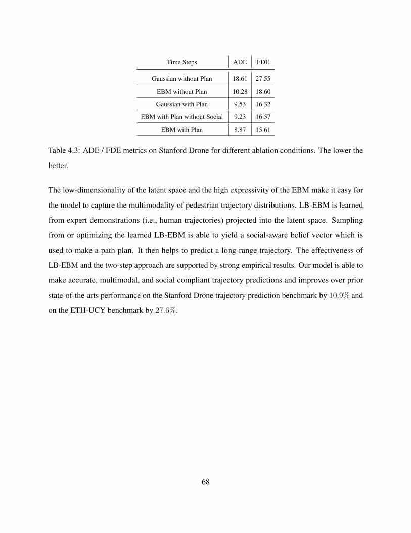
Time Steps ADE FDE

Gaussian without Plan 18.61 27.55

EBM without Plan 10.28 18.60

Gaussian with Plan 9.53 16.32

EBM with Plan without Social 9.23 16.57

EBM with Plan 8.87 15.61

Table 4.3: ADE / FDE metrics on Stanford Drone for different ablation conditions. The lower the

better.

The low-dimensionality of the latent space and the high expressivity of the EBM make it easy for

the model to capture the multimodality of pedestrian trajectory distributions. LB-EBM is learned

from expert demonstrations (i.e., human trajectories) projected into the latent space. Sampling

from or optimizing the learned LB-EBM is able to yield a social-aware belief vector which is

used to make a path plan. It then helps to predict a long-range trajectory. The effectiveness of

LB-EBM and the two-step approach are supported by strong empirical results. Our model is able to

make accurate, multimodal, and social compliant trajectory predictions and improves over prior

state-of-the-arts performance on the Stanford Drone trajectory prediction benchmark by 10.9% and

on the ETH-UCY benchmark by 27.6%.

68

CHAPTER APPENDIX

4.A Learning

4.A.1 Model formulation

Recall thatXXX = {xxxi, i = 1, ..., n} indicates the past trajectories of all agents in the scene. Similarly,

YYY indicates all future trajectories. ZZZ represents the latent belief of agents. PPP denotes the plans. We

model the following generative model,

pψ(ZZZ,PPP ,YYY |XXX) = pα(ZZZ|XXX)︸ ︷︷ ︸LB-EBM

Plan︷ ︸︸ ︷pβ(PPP |ZZZ,XXX) pγ(YYY |PPP ,XXX)︸ ︷︷ ︸

Prediction

. (4.16)

4.A.2 Maximum likelihood learning

Let qdata(PPP ,YYY |XXX)qdata(XXX) be the data distribution that generates the (multi-agent) trajectory

example, (PPP ,YYY ,XXX), in a single scene. The learning of parameters ψ of the generative model

pψ(ZZZ,PPP ,YYY |XXX) can be based on minψDKL(qdata(PPP ,YYY |XXX) ∥ pψ(PPP ,YYY |XXX)) where DKL(q(x) ∥ p(x)) =

Eq[log q(x)/p(x)] is the Kullback-Leibler divergence between q and p (or from q to p since

DKL(q(x) ∥ p(x)) is asymmetric). If we observe training examples {(PPP j,YYY j,XXXj), j = 1, .., N} ∼

qdata(PPP ,YYY |XXX)qdata(XXX), the above minimization can be approximated by maximizing the log-

likelihood,

N∑j=1

log pψ(PPP j,YYY j|XXXj) =N∑j=1

log

∫ZZZj

pψ(ZZZj,PPP j,YYY j|XXXj) (4.17)

69

which leads to the maximum likelihood estimate (MLE). Then the gradient of the log-likelihood of

a single scene can be computed according to the following identity,

∇ψ log pψ(PPP ,YYY |XXX) =1

pψ(PPP ,YYY |XXX)∇ψ

∫ZZZ

pψ(ZZZ,PPP ,YYY |XXX) (4.18)

=

∫ZZZ

pψ(ZZZ,PPP ,YYY |XXX)

pψ(PPP ,YYY |XXX)∇ψ log pψ(ZZZ,PPP ,YYY |XXX) (4.19)

=

∫ZZZ

pψ(ZZZ|XXX)pψ(PPP |ZZZ,XXX)pψ(YYY |PPP ,XXX)

pψ(PPP |XXX)pψ(YYY |PPP ,XXX)∇ψ log pψ(ZZZ,PPP ,YYY |XXX) (4.20)

= Epψ(ZZZ|PPP ,XXX) ∇ψ log pψ(ZZZ,PPP ,YYY |XXX). (4.21)

The above expectation involves the posterior pψ(ZZZ|PPP ,XXX) which is however intractable.

4.A.3 Variational learning

Due to the intractiablity of the maximum likelihood learning, we derive a tractable variational

objective. Define

qϕ(ZZZ,PPP ,YYY |XXX) = qdata(PPP ,YYY |XXX)qϕ(ZZZ|PPP ,XXX) (4.22)

where qϕ(ZZZ|PPP ,XXX) is a tractable variational distribution, particularly, a Gaussian with a diagnoal

covariance matrix used in this work. Then our variational objective is defined to be the tractable KL

divergence below,

DKL(qϕ(ZZZ,PPP ,YYY |XXX) ∥ pψ(ZZZ,PPP ,YYY |XXX)) (4.23)

where qϕ(ZZZ,PPP ,YYY |XXX) involves either the data distribution or the tractable variational distribution.

Notice that,

DKL(qϕ(ZZZ,PPP ,YYY |XXX) ∥ pψ(ZZZ,PPP ,YYY |XXX)) (4.24)

= DKL(qdata(PPP ,YYY |XXX) ∥ pψ(PPP ,YYY |XXX)) (4.25)

+ DKL(qϕ(ZZZ|PPP ,XXX) ∥ pψ(ZZZ|PPP ,XXX)) (4.26)

which is an upper bound of DKL(qdata(PPP ,YYY |XXX) ∥ pψ(PPP ,YYY |XXX)) due to the non-negativity of KL

divergence, in particular, DKL(qϕ(ZZZ|PPP ,XXX) ∥ pψ(ZZZ|PPP ,XXX)), and equivalently a lower bound of the

log-likelihood.

70

We next unpack the generative model pψ(ZZZ,PPP ,YYY |XXX) and have,

DKL(qϕ(ZZZ,PPP ,YYY |XXX) ∥ pψ(ZZZ,PPP ,YYY |XXX)) (4.27)

= DKL(qdata(PPP ,YYY |XXX)qϕ(ZZZ|PPP ,XXX) ∥ pα(ZZZ|XXX)pβ(PPP |ZZZ,XXX)pγ(YYY |PPP ,XXX)) (4.28)

= Eqdata(XXX) Eqdata(PPP ,YYY |XXX)qϕ(ZZZ|PPP ,XXX) logqϕ(ZZZ|PPP ,XXX)

pα(ZZZ|XXX)(4.29)

+ Eqdata(XXX) Eqdata(PPP ,YYY |XXX)qϕ(ZZZ|PPP ,XXX) logqdata(PPP |YYY ,XXX)

pβ(PPP |ZZZ,XXX)(4.30)

+ Eqdata(XXX) Eqdata(PPP ,YYY |XXX)qϕ(ZZZ|PPP ,XXX) logqdata(YYY |XXX)

pγ(YYY |PPP ,XXX)(4.31)

Expressions 4.29, 4.30, 4.31 are the major objectives for learning the LB-EBM, plan, and prediction

modules respectively. They are the ”major” but not ”only” ones since the whole network is trained

end-to-end and gradients from one module can flow to the other. We next unpack each of the

objectives (where Eqdata(XXX) is omitted for notational simplicity).

Expression 4.29 drives the learning of the LB-EBM.

Eqdata(PPP ,YYY |XXX)qϕ(ZZZ|PPP ,XXX) logqϕ(ZZZ|PPP ,XXX)

pα(ZZZ|XXX)(4.32)

= Eqdata(PPP ,YYY |XXX)qϕ(ZZZ|PPP ,XXX) logqϕ(ZZZ|PPP ,XXX)

p0(ZZZ) exp[−Cα(ZZZ,XXX)]/Zα(XXX)(4.33)

= DKL(qϕ(ZZZ|PPP ,XXX) ∥ p0(ZZZ)) (4.34)

+ Eqdata(PPP ,YYY |XXX)qϕ(ZZZ|PPP ,XXX)Cα(ZZZ,XXX) + logZα(XXX) (4.35)

where Zα(XXX) =∫ZZZexp(−Cα(ZZZ,XXX))p0(ZZZ) = Ep0(ZZZ)(−Cα(ZZZ,XXX)).

Let J (α) = Eqdata(XXX) Eqdata(PPP ,YYY |XXX)qϕ(ZZZ|PPP ,XXX)Cα(ZZZ,XXX) + Eqdata(XXX) logZα(XXX), which is the ob-

jective for LB-EBM learning and follows the philosophy of IRL. And its gradient is,

∇αJ (α) =Eqdata(XXX) Eqdata(PPP ,YYY |XXX)qϕ(ZZZ|PPP ,XXX)[∇αCα(ZZZ,XXX)] (4.36)

− Eqdata(XXX) Epα(ZZZ|XXX)[∇αCα(ZZZ,XXX)] (4.37)

71

Thus, α is learned based on the distributional difference between the expert beliefs and those

sampled from the current LB-EBM. The expectations over qdata(XXX) and qdata(PPP ,YYY |XXX) are approxi-

mated with a mini-batch from the empirical data distribution. The expectation over qϕ(ZZZ|PPP ,XXX) is

approximated with samples from the variational distribution through the reparameterization trick.

The expectation over pα(ZZZ|XXX) is approximated with samples from Langevin dynamics guided by

the current cost function.

Expression 4.30 drives the learning of the plan module.

(4.30) = −Eqdata(XXX) Eqdata(PPP ,YYY |XXX)qϕ(ZZZ|PPP ,XXX) log pβ(PPP |ZZZ,XXX)−H(PPP |YYY ,XXX) (4.38)

where H(PPP |YYY ,XXX) is the conditional entropy of qdata(PPP |XXX,YYY ) and is a constant with respect to

the model parameters. Thus minimizing 4.30 is equivalent to maximizing the log-likelihood of

pβ(PPP |ZZZ,XXX).

Expression 4.31 drives the learning of the prediction module.

(4.31) = −Eqdata(XXX) Eqdata(PPP ,YYY |XXX)qϕ(ZZZ|PPP ,XXX) log pγ(YYY |PPP ,XXX)−H(YYY |XXX) (4.39)

where H(YYY |XXX) is the conditional entropy of qdata(YYY |XXX) and is constant with respect to the model

parameters. We can minimize Expression 4.39 for optimizing the prediction module. In the learning,

PPP is sampled from the data distribution qdata(PPP ,YYY |XXX). In practice, we find sampling PPP from the

generative model pβ(PPP |ZZZ,XXX) instead facilitates learning of other modules, leading to improved

performance. The objective for learning the prediction module then becomes,

− Eqdata(XXX) Eqdata(YYY |XXX) Eqϕ(ZZZ|XXX) Epβ(PPP |ZZZ,XXX) log pγ(YYY |PPP ,XXX) (4.40)

where

Eqϕ(ZZZ|XXX) =

∫PPP

qdata(PPP |YYY ,XXX)qϕ(ZZZ|PPP ,XXX) (4.41)

= Eqdata(PPP |YYY ,XXX) qϕ(ZZZ|PPP ,XXX). (4.42)

72

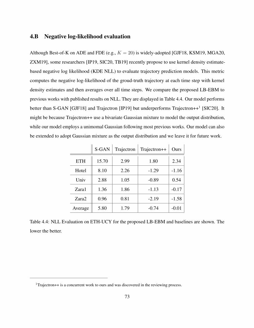
4.B Negative log-likelihood evaluation

Although Best-of-K on ADE and FDE (e.g., K = 20) is widely-adopted [GJF18, KSM19, MGA20,

ZXM19], some researchers [IP19, SIC20, TB19] recently propose to use kernel density estimate-

based negative log likelihood (KDE NLL) to evaluate trajectory prediction models. This metric

computes the negative log-likelihood of the groud-truth trajectory at each time step with kernel

density estimates and then averages over all time steps. We compare the proposed LB-EBM to

previous works with published results on NLL. They are displayed in Table 4.4. Our model performs

better than S-GAN [GJF18] and Trajectron [IP19] but underperforms Trajectron++1 [SIC20]. It

might be because Trajectron++ use a bivariate Gaussian mixture to model the output distribution,

while our model employs a unimomal Gaussian following most previous works. Our model can also

be extended to adopt Gaussian mixture as the output distribution and we leave it for future work.

S-GAN Trajectron Trajectron++ Ours

ETH 15.70 2.99 1.80 2.34

Hotel 8.10 2.26 -1.29 -1.16

Univ 2.88 1.05 -0.89 0.54

Zara1 1.36 1.86 -1.13 -0.17

Zara2 0.96 0.81 -2.19 -1.58

Average 5.80 1.79 -0.74 -0.01

Table 4.4: NLL Evaluation on ETH-UCY for the proposed LB-EBM and baselines are shown. The

lower the better.

1Trajectron++ is a concurrent work to ours and was discovered in the reviewing process.

73

CHAPTER 5

Latent Space Energy-Based Model of Symbol-Vector Coupling

5.1 Introduction

In the previous chapters, we have established the effectiveness of latent space EBM, a principled

unification of EBM and generator model. However, the learned latent space is generally not well-

structured. And the model cannot be directly applied to classification, which is a widespread task.

In this chapter, we further seek to integrate latent space EBM and discriminative model, with which

we reach the goal of developing a probabilistic model that unifies EBM, generator model, and

discriminative model. The unification is done by formulating the energy term as a coupling of a

continuous latent vector and a symbolic one-hot vector, so that discrete category can be inferred

from the observed example based on the continuous latent vector. We also develop an objective,

following the principle of information bottleneck, which encourages the continuous latent vector

to extract information from the observed example that is informative of the underlying category.

We study this model in the domain of natural language and explore its applications in controlled

generation and semi-supervised classification.

5.2 Motivation

Generative models for text generation is of vital importance in a wide range of real world appli-

cations such as dialog system [YGT13] and machine translation [BDD93]. Impressive progress

has been achieved with the development of neural generative models [SSB16, ZZE17, ZLE18,

ZXS16, LLB17, GAS18, ZKZ18] . However, most of prior methods focus on the improvement of

74

text generation quality such as fluency and diversity. Besides the quality, the interpretability or

controllability of text generation process is also critical for real world applications. Several recent

papers recruit deep latent variable models for interpretable text generation where the latent space is

learned to capture interpretable structures such as topics and dialog actions which are then used to

guide text generation [WGX19, ZLE18].

Deep latent variable models map a latent vector to the observed example such as a piece of

text. Earlier methods [KW14, RMW14, BVV16] utilize a continuous latent space. Although it is

able to generate text of high quality, it is not suitable for modeling interpretable discrete attributes

such as topics and dialog actions. A recent paper [ZLE18] proposes to use a discrete latent space

in order to capture dialog actions and has shown promising interpretability of dialog utterance

generation. A discrete latent space nevertheless encodes limited information and thus might limit the

expressiveness of the generative model. To address this issue, [SZM20] proposes to use Gaussian

mixture VAE (variational auto-encoder) which has a latent space with both continuous and discrete

latent variables. By including a dispersion term to avoid the modes of the Gaussian mixture to

collapse into a single mode, the model produces promising results on interpretable generation of

dialog utterances.

To improve the expressivity of the latent space and the generative model as a whole, [PHN20]

recently proposes to learn an energy-based model (EBM) in the latent space, where the EBM serves

as a prior model for the latent vector. Both the EBM prior and the generator network are learned

jointly by maximum likelihood or its approximate variants. The latent space EBM has been applied

to text modeling, image modeling, and molecule generation, and significantly improves over VAEs

with Gaussian prior, mixture prior and other flexible priors. [ASK20] generalizes this model to a

multi-layer latent variable model with a large-scale generator network and achieves state-of-the-art

generation performance on images.

Moving EBM from data space to latent space allows the EBM to stand on an already expressive

generator model, and the EBM prior can be considered a correction of the non-informative uniform

or isotropic Gaussian prior of the generative model. Due to the low dimensionality of the latent

75

space, the EBM can be parametrized by a very small network, and yet it can capture regularities and

rules in the data effectively (and implicitly).

In this work, we attempt to leverage the high expressivity of EBM prior for text modeling and

learn a well-structured latent space for both interpretable generation and text classification. Thus,

we formulate a new prior distribution which couples continuous latent variables (i.e., vector) for

generation and discrete latent variables (i.e., symbol) for structure induction. We call our model

Symbol-Vector Coupling Energy-Based Model (SVEBM).

Two key differences of the current model from [PHN20] enable incorporation of information

bottleneck [TPB00], which encourages the continuous latent vector to extract information from

the observed example that is informative of the underlying structure. First, unlike [PHN20] where

the posterior inference is done with short-run MCMC sampling, we learn an amortized inference

network which can be conveniently optimized. Second, due to the coupling formulation of the

continuous latent vector and the symbolic one-hot vector, given the inferred continuous vector,

the symbol or category can be inferred from it via a standard softmax classifier (see Section 5.3.1

for more details). The model can be learned in unsupervised setting where no category labels

are provided. The symbol-vector coupling, the generator network, and the inference network are

learned jointly by maximizing the variational lower bound of the log-likelihood. The model can also

be learned in semi-supervised setting where the category labels are provided for a subset of training

examples. The coupled symbol-vector allows the learned model to generate text from the latent

vector controlled by the symbol. Moreover, text classification can be accomplished by inferring the

symbol based on the continuous vector that is inferred from the observed text.

The contributions of this chapter is summarized as follows. (1) We propose a symbol-vector

coupling EBM in the latent space, which is capable of both unsupervised and semi-supervised

learning. (2) We develop a regularization of the model based on the information bottleneck principle.

(3) Our experiments demonstrate that the proposed model learns well-structured and meaningful

latent space, allowing for interpretable text generation and effective text classification.

76

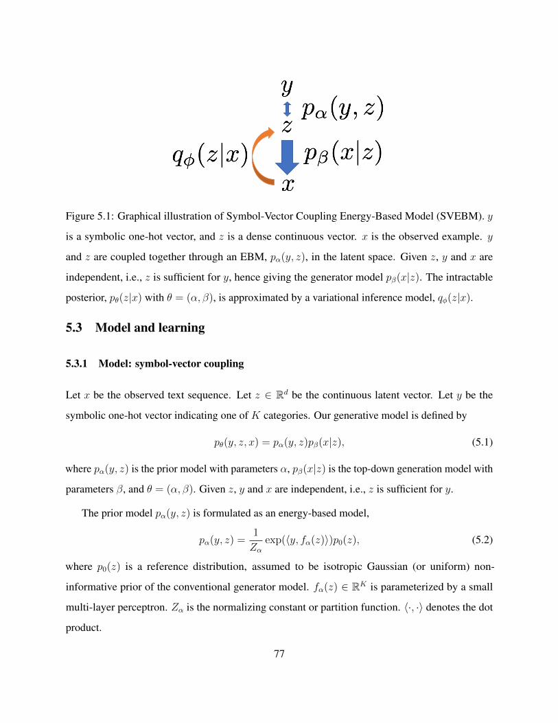
Figure 5.1: Graphical illustration of Symbol-Vector Coupling Energy-Based Model (SVEBM). y

is a symbolic one-hot vector, and z is a dense continuous vector. x is the observed example. y

and z are coupled together through an EBM, pα(y, z), in the latent space. Given z, y and x are

independent, i.e., z is sufficient for y, hence giving the generator model pβ(x|z). The intractable

posterior, pθ(z|x) with θ = (α, β), is approximated by a variational inference model, qϕ(z|x).

5.3 Model and learning

5.3.1 Model: symbol-vector coupling

Let x be the observed text sequence. Let z ∈ Rd be the continuous latent vector. Let y be the

symbolic one-hot vector indicating one of K categories. Our generative model is defined by

pθ(y, z, x) = pα(y, z)pβ(x|z), (5.1)

where pα(y, z) is the prior model with parameters α, pβ(x|z) is the top-down generation model with

parameters β, and θ = (α, β). Given z, y and x are independent, i.e., z is sufficient for y.

The prior model pα(y, z) is formulated as an energy-based model,

pα(y, z) =1

Zαexp(⟨y, fα(z)⟩)p0(z), (5.2)

where p0(z) is a reference distribution, assumed to be isotropic Gaussian (or uniform) non-

informative prior of the conventional generator model. fα(z) ∈ RK is parameterized by a small

multi-layer perceptron. Zα is the normalizing constant or partition function. ⟨·, ·⟩ denotes the dot

product.

77

The energy term ⟨y, fα(z)⟩ in Equation (5.2) forms an associative memory that couples the

symbol y and the dense vector z. Given z,

pα(y|z) ∝ exp(⟨y, fα(z)⟩), (5.3)

i.e., a softmax classifier, where fα(z) provides the K logit scores for the K categories. Marginally,

pα(z) =1

Zαexp(Fα(z))p0(z), (5.4)

where the marginal energy term

Fα(z) = log∑y

exp(⟨y, fα(z)⟩), (5.5)

i.e., the so-called log-sum-exponential form. The summation can be easily computed because we

only need to sum over K different values of the one-hot y.

The above prior model pα(y, z) stands on a generation model pβ(x|z). For text modeling, let

x = (x(t), t = 1, ..., T ) where x(t) is the t-th token. Following previous text VAE model [BVV16],

we define pβ(x|z) as a conditional autoregressive model,

pβ(x|z) =T∏t=1

pβ(x(t)|x(1), ..., x(t−1), z) (5.6)

which is parameterized by a recurrent network with parameters β. See Figure 5.1 for a graphical

illustration of our model.

5.3.2 Prior and posterior sampling: symbol-aware continuous vector computation

Sampling from the prior pα(z) and the posterior pθ(z|x) can be accomplished by Langevin dynamics.

For prior sampling from pα(z), Langevin dynamics iterates

zt+1 = zt + s∇z log pα(zt) +√2set, (5.7)

where et ∼ N (0, Id), s is the step size, and the gradient is computed by

∇z log pα(z) = Epα(y|z)[∇z log pα(y, z)]

= Epα(y|z)[⟨y,∇zfα(z)⟩], (5.8)

78

where the gradient computation involves averaging ∇zfα(z) over the softmax classification proba-

bilities pα(y|z) in Equation (5.3). Thus the sampling of the continuous dense vector z is aware of

the symbolic y.

Posterior sampling from pθ(z|x) follows a similar scheme, where

∇z log pθ(z|x) = Epα(y|z)[⟨y,∇zfα(z)⟩] +∇z log pβ(x|z). (5.9)

When the dynamics is reasoning about x by sampling the dense continuous vector z from pθ(z|x),

it is aware of the symbolic y via the softmax pα(y|z).

Thus (y, z) forms a coupling between symbol and dense vector, which gives the name of our

model, Symbol-Vector Coupling Energy-Based Model (SVEBM).

[PHN20] proposes to use prior and posterior sampling for maximum likelihood learning. Due

to the low-dimensionality of the latent space, MCMC sampling is affordable and mixes well.

5.3.3 Amortizing posterior sampling and variational learning

Comparing prior and posterior sampling, prior sampling is particularly affordable, because fα(z) is

a small network. In comparison, ∇z log pβ(x|z) in the posterior sampling requires back-propagation

through the generator network, which can be more expensive. Therefore we shall amortize the

posterior sampling from pθ(z|x) by an inference network, and we continue to use MCMC for prior

sampling.

Specifically, following VAE [KW14], we recruit an inference network qϕ(z|x) to approximate

the true posterior pθ(z|x), in order to amortize posterior sampling. Following VAE, we learn the

inference model qϕ(z|x) and the top-down model pθ(y, z, x) in Equation (5.1) jointly.

For unlabeled x, the log-likelihood log pθ(x) is lower bounded by the evidence lower bound

(ELBO),

ELBO(x|θ, ϕ) = log pθ(x)− DKL(qϕ(z|x)∥pθ(z|x))

= Eqϕ(z|x) [log pβ(x|z)]− DKL(qϕ(z|x)∥pα(z)), (5.10)

79

where DKL denotes the Kullback-Leibler divergence.

For the prior model, the learning gradient is

∇α ELBO = Eqϕ(z|x)[∇αFα(z)]− Epα(z)[∇αFα(z)], (5.11)

where Fα(z) is defined by (5.5), Eqϕ(z|x) is approximated by samples from the inference network,

and Epα(z) is approximated by persistent MCMC samples from the prior.

Let ψ = {β, ϕ} collect the parameters of the inference (encoder) and generator (decoder)

models. The learning gradients for the two models are

∇ψ ELBO = ∇ψ Eqϕ(z|x)[log pβ(x|z)]

−∇ψ DKL(qϕ(z|x)∥p0(z)) +∇ψ Eqϕ(z|x) [Fα(z)], (5.12)

where p0(z) is the reference distribution in Equation (5.2), and DKL(qϕ(z|x)∥p0(z)) is tractable.

The expectations in the other two terms are approximated by samples from the inference network

qϕ(z|x) with reparametrization trick [KW14]. Compared to the original VAE, we only need to

include the extra Fα(z) term in Equation (5.12), while logZα is a constant that can be discarded.

This expands the scope of VAE where the top-down model is a latent EBM.

As mentioned above, we shall not amortize the prior sampling from pα(z) due to its simplicity.

Sampling pα(z) is only needed in the training stage, but is not required in the testing stage.

5.3.4 Two joint distributions

Let qdata(x) be the data distribution that generates x. For variational learning, we maximize the

averaged ELBO: Eqdata(x)[ELBO(x|θ, ϕ)], where Eqdata(x) can be approximated by averaging over

the training examples. Maximizing Eqdata(x)[ELBO(x|θ, ϕ)] over (θ, ϕ) is equivalent to minimizing

the following objective function over (θ, ϕ)

DKL(qdata(x)∥pθ(x)) + Eqdata(x)[DKL(qϕ(z|x)∥pθ(z|x))]

= DKL(qdata(x)qϕ(z|x)∥pα(z)pβ(x|z)). (5.13)

80

The right hand side is the KL-divergence between two joint distributions: Qϕ(x, z) = qdata(x)qϕ(z|x),

and Pθ(x, z) = pα(z)pβ(x|z). The reason we use notation q for the data distribution qdata(x) is

for notation consistency. Thus VAE can be considered as joint minimization of DKL(Qϕ∥Pθ) over

(θ, ϕ). Treating (x, z) as the complete data, Qϕ can be considered the complete data distribution,

while Pθ is the model distribution of the complete data.

For the distribution Qϕ(x, z), we can define the following quantities.

qϕ(z) = Eqdata(x)[qϕ(z|x)] =∫Qϕ(x, z)dx (5.14)

is the aggregated posterior distribution and the marginal distribution of z under Qϕ. H(z) =

−Eqϕ(z)[log qϕ(z)] is the entropy of the aggregated posterior qϕ(z).

H(z|x) = −EQϕ(x,z)[log qϕ(z|x)] is the conditional entropy of z given x under the variational

inference distribution qϕ(z|x).

I(x, z) = H(z)−H(z|x)

= −Eqϕ(z)[log qϕ(z)] + EQϕ(x,z)[log qϕ(z|x)] (5.15)

is the mutual information between x and z under Qϕ.

It can be shown that the VAE objective in Equation (5.13) can be written as

DKL(Qϕ(x, z)∥Pθ(x, z))

= −H(x)− EQϕ(x,z)[log pβ(x|z)] + I(x, z) + DKL(qϕ(z)∥pα(z)), (5.16)

where H(x) = −Eqdata(x)[log qdata(x)] is the entropy of the data distribution and is fixed.

5.3.5 Information bottleneck

Due to the coupling of y and z (see Equations (5.2) and (5.3)), a learning objective with information

bottleneck can be naturally developed as a simple modification of the VAE objective in Equations

81

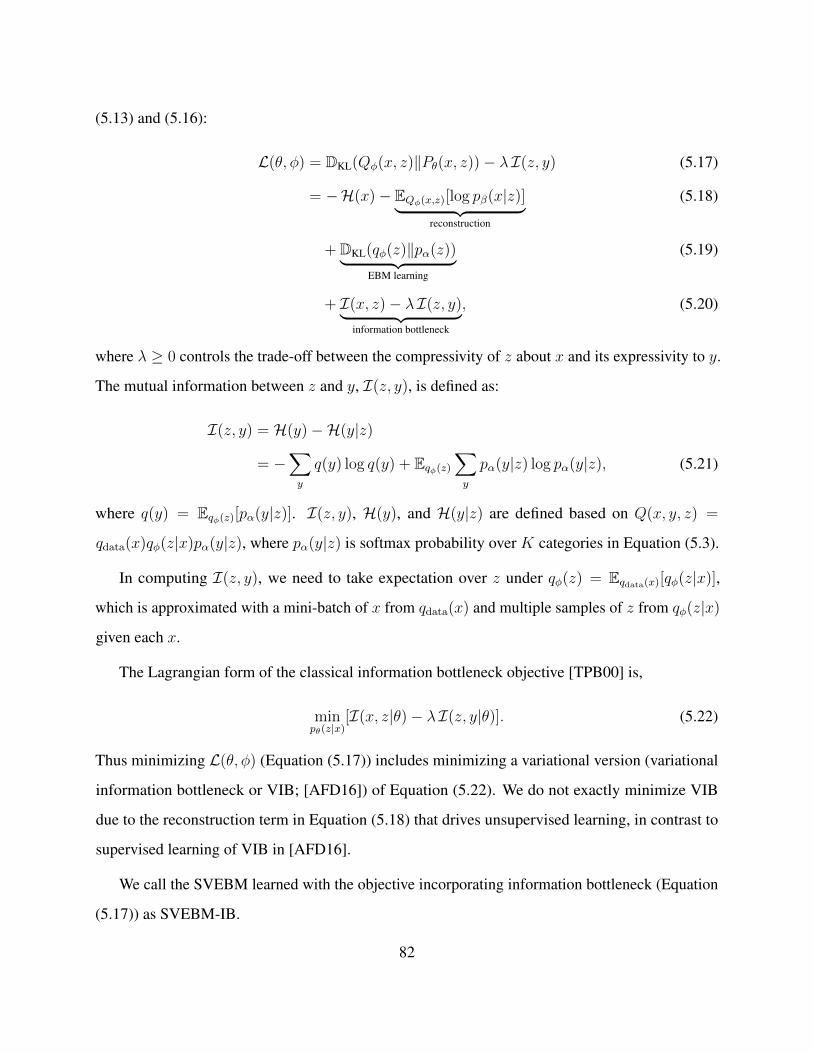
(5.13) and (5.16):

L(θ, ϕ) = DKL(Qϕ(x, z)∥Pθ(x, z))− λ I(z, y) (5.17)

= −H(x)− EQϕ(x,z)[log pβ(x|z)]︸ ︷︷ ︸reconstruction

(5.18)

+ DKL(qϕ(z)∥pα(z))︸ ︷︷ ︸EBM learning

(5.19)

+ I(x, z)− λ I(z, y)︸ ︷︷ ︸information bottleneck

, (5.20)

where λ ≥ 0 controls the trade-off between the compressivity of z about x and its expressivity to y.

The mutual information between z and y, I(z, y), is defined as:

I(z, y) = H(y)−H(y|z)

= −∑y

q(y) log q(y) + Eqϕ(z)∑y

pα(y|z) log pα(y|z), (5.21)

where q(y) = Eqϕ(z)[pα(y|z)]. I(z, y), H(y), and H(y|z) are defined based on Q(x, y, z) =

qdata(x)qϕ(z|x)pα(y|z), where pα(y|z) is softmax probability over K categories in Equation (5.3).

In computing I(z, y), we need to take expectation over z under qϕ(z) = Eqdata(x)[qϕ(z|x)],

which is approximated with a mini-batch of x from qdata(x) and multiple samples of z from qϕ(z|x)

given each x.

The Lagrangian form of the classical information bottleneck objective [TPB00] is,

minpθ(z|x)

[I(x, z|θ)− λ I(z, y|θ)]. (5.22)

Thus minimizing L(θ, ϕ) (Equation (5.17)) includes minimizing a variational version (variational

information bottleneck or VIB; [AFD16]) of Equation (5.22). We do not exactly minimize VIB

due to the reconstruction term in Equation (5.18) that drives unsupervised learning, in contrast to

supervised learning of VIB in [AFD16].

We call the SVEBM learned with the objective incorporating information bottleneck (Equation

(5.17)) as SVEBM-IB.

82

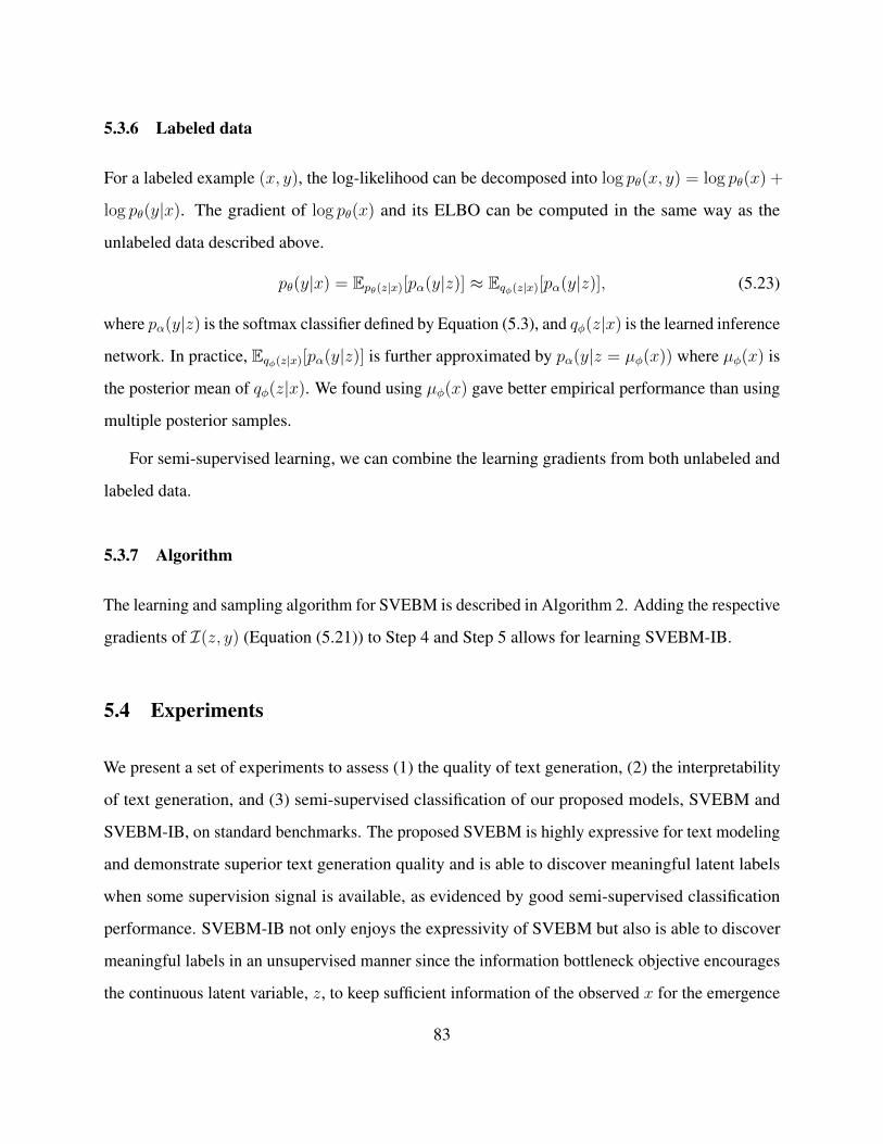
5.3.6 Labeled data

For a labeled example (x, y), the log-likelihood can be decomposed into log pθ(x, y) = log pθ(x) +

log pθ(y|x). The gradient of log pθ(x) and its ELBO can be computed in the same way as the

unlabeled data described above.

pθ(y|x) = Epθ(z|x)[pα(y|z)] ≈ Eqϕ(z|x)[pα(y|z)], (5.23)

where pα(y|z) is the softmax classifier defined by Equation (5.3), and qϕ(z|x) is the learned inference

network. In practice, Eqϕ(z|x)[pα(y|z)] is further approximated by pα(y|z = µϕ(x)) where µϕ(x) is

the posterior mean of qϕ(z|x). We found using µϕ(x) gave better empirical performance than using

multiple posterior samples.

For semi-supervised learning, we can combine the learning gradients from both unlabeled and

labeled data.

5.3.7 Algorithm

The learning and sampling algorithm for SVEBM is described in Algorithm 2. Adding the respective

gradients of I(z, y) (Equation (5.21)) to Step 4 and Step 5 allows for learning SVEBM-IB.

5.4 Experiments

We present a set of experiments to assess (1) the quality of text generation, (2) the interpretability

of text generation, and (3) semi-supervised classification of our proposed models, SVEBM and

SVEBM-IB, on standard benchmarks. The proposed SVEBM is highly expressive for text modeling

and demonstrate superior text generation quality and is able to discover meaningful latent labels

when some supervision signal is available, as evidenced by good semi-supervised classification

performance. SVEBM-IB not only enjoys the expressivity of SVEBM but also is able to discover

meaningful labels in an unsupervised manner since the information bottleneck objective encourages

the continuous latent variable, z, to keep sufficient information of the observed x for the emergence

83

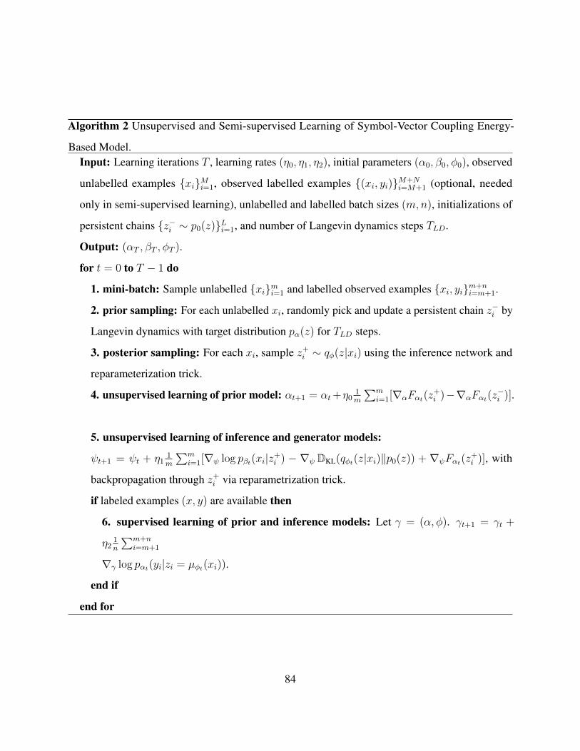
Algorithm 2 Unsupervised and Semi-supervised Learning of Symbol-Vector Coupling Energy-

Based Model.Input: Learning iterations T , learning rates (η0, η1, η2), initial parameters (α0, β0, ϕ0), observed

unlabelled examples {xi}Mi=1, observed labelled examples {(xi, yi)}M+Ni=M+1 (optional, needed

only in semi-supervised learning), unlabelled and labelled batch sizes (m,n), initializations of

persistent chains {z−i ∼ p0(z)}Li=1, and number of Langevin dynamics steps TLD.

Output: (αT , βT , ϕT ).

for t = 0 to T − 1 do

1. mini-batch: Sample unlabelled {xi}mi=1 and labelled observed examples {xi, yi}m+ni=m+1.

2. prior sampling: For each unlabelled xi, randomly pick and update a persistent chain z−i by

Langevin dynamics with target distribution pα(z) for TLD steps.

3. posterior sampling: For each xi, sample z+i ∼ qϕ(z|xi) using the inference network and

reparameterization trick.

4. unsupervised learning of prior model: αt+1 = αt+η01m

∑mi=1[∇αFαt(z

+i )−∇αFαt(z

−i )].

5. unsupervised learning of inference and generator models:

ψt+1 = ψt + η11m

∑mi=1[∇ψ log pβt(xi|z+i ) − ∇ψ DKL(qϕt(z|xi)∥p0(z)) + ∇ψFαt(z

+i )], with

backpropagation through z+i via reparametrization trick.

if labeled examples (x, y) are available then

6. supervised learning of prior and inference models: Let γ = (α, ϕ). γt+1 = γt +

η21n

∑m+ni=m+1

∇γ log pαt(yi|zi = µϕt(xi)).

end if

end for

84

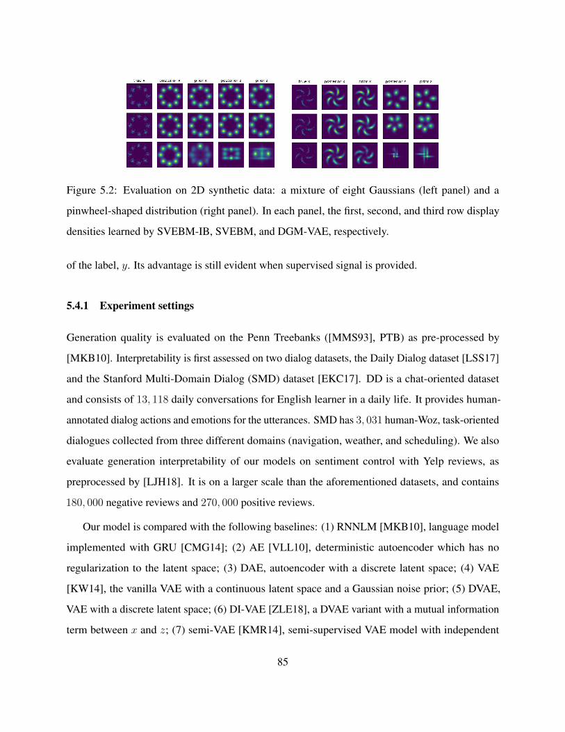
Figure 5.2: Evaluation on 2D synthetic data: a mixture of eight Gaussians (left panel) and a

pinwheel-shaped distribution (right panel). In each panel, the first, second, and third row display

densities learned by SVEBM-IB, SVEBM, and DGM-VAE, respectively.

of the label, y. Its advantage is still evident when supervised signal is provided.

5.4.1 Experiment settings

Generation quality is evaluated on the Penn Treebanks ([MMS93], PTB) as pre-processed by

[MKB10]. Interpretability is first assessed on two dialog datasets, the Daily Dialog dataset [LSS17]

and the Stanford Multi-Domain Dialog (SMD) dataset [EKC17]. DD is a chat-oriented dataset

and consists of 13, 118 daily conversations for English learner in a daily life. It provides human-

annotated dialog actions and emotions for the utterances. SMD has 3, 031 human-Woz, task-oriented

dialogues collected from three different domains (navigation, weather, and scheduling). We also

evaluate generation interpretability of our models on sentiment control with Yelp reviews, as

preprocessed by [LJH18]. It is on a larger scale than the aforementioned datasets, and contains

180, 000 negative reviews and 270, 000 positive reviews.

Our model is compared with the following baselines: (1) RNNLM [MKB10], language model

implemented with GRU [CMG14]; (2) AE [VLL10], deterministic autoencoder which has no

regularization to the latent space; (3) DAE, autoencoder with a discrete latent space; (4) VAE

[KW14], the vanilla VAE with a continuous latent space and a Gaussian noise prior; (5) DVAE,

VAE with a discrete latent space; (6) DI-VAE [ZLE18], a DVAE variant with a mutual information

term between x and z; (7) semi-VAE [KMR14], semi-supervised VAE model with independent

85

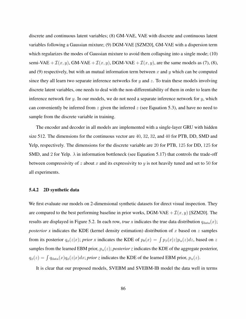
discrete and continuous latent variables; (8) GM-VAE, VAE with discrete and continuous latent

variables following a Gaussian mixture; (9) DGM-VAE [SZM20], GM-VAE with a dispersion term

which regularizes the modes of Gaussian mixture to avoid them collapsing into a single mode; (10)

semi-VAE + I(x, y), GM-VAE + I(x, y), DGM-VAE + I(x, y), are the same models as (7), (8),

and (9) respectively, but with an mutual information term between x and y which can be computed

since they all learn two separate inference networks for y and z. To train these models involving

discrete latent variables, one needs to deal with the non-differentiability of them in order to learn the

inference network for y. In our models, we do not need a separate inference network for y, which

can conveniently be inferred from z given the inferred z (see Equation 5.3), and have no need to

sample from the discrete variable in training.

The encoder and decoder in all models are implemented with a single-layer GRU with hidden

size 512. The dimensions for the continuous vector are 40, 32, 32, and 40 for PTB, DD, SMD and

Yelp, respectively. The dimensions for the discrete variable are 20 for PTB, 125 for DD, 125 for

SMD, and 2 for Yelp. λ in information bottleneck (see Equation 5.17) that controls the trade-off

between compressivity of z about x and its expressivity to y is not heavily tuned and set to 50 for

all experiments.

5.4.2 2D synthetic data

We first evaluate our models on 2-dimensional synthetic datasets for direct visual inspection. They

are compared to the best performing baseline in prior works, DGM-VAE + I(x, y) [SZM20]. The

results are displayed in Figure 5.2. In each row, true x indicates the true data distribution qdata(x);

posterior x indicates the KDE (kernel density estimation) distribution of x based on z samples

from its posterior qϕ(z|x); prior x indicates the KDE of pθ(x) =∫pβ(x|z)pα(z)dz, based on z

samples from the learned EBM prior, pα(z); posterior z indicates the KDE of the aggregate posterior,

qϕ(z) =∫qdata(x)qϕ(z|x)dx; prior z indicates the KDE of the learned EBM prior, pα(z).

It is clear that our proposed models, SVEBM and SVEBM-IB model the data well in terms

86

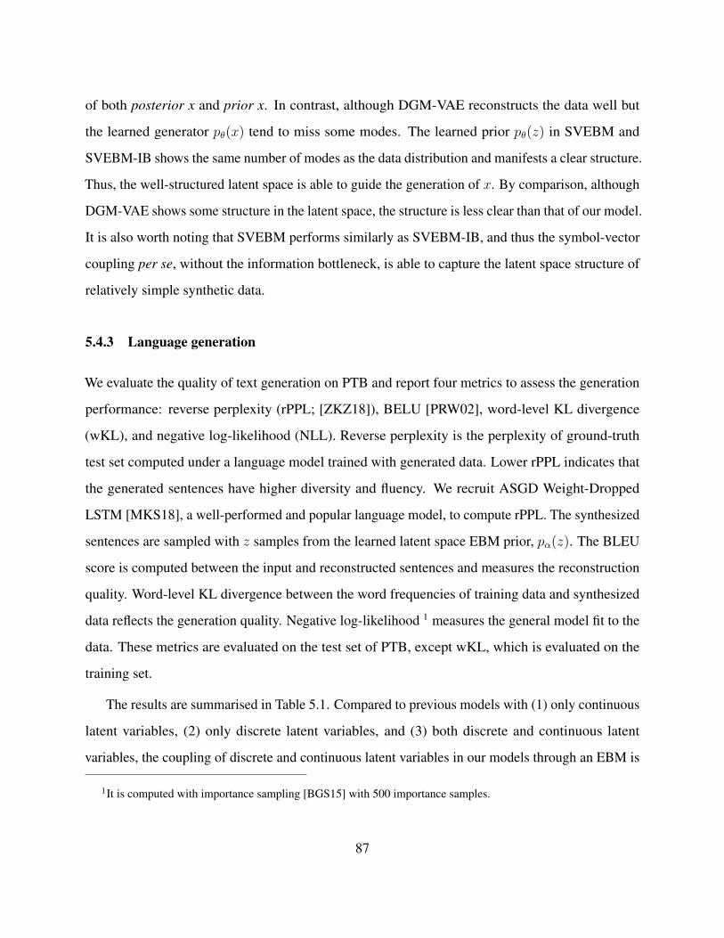
of both posterior x and prior x. In contrast, although DGM-VAE reconstructs the data well but

the learned generator pθ(x) tend to miss some modes. The learned prior pθ(z) in SVEBM and

SVEBM-IB shows the same number of modes as the data distribution and manifests a clear structure.

Thus, the well-structured latent space is able to guide the generation of x. By comparison, although

DGM-VAE shows some structure in the latent space, the structure is less clear than that of our model.

It is also worth noting that SVEBM performs similarly as SVEBM-IB, and thus the symbol-vector

coupling per se, without the information bottleneck, is able to capture the latent space structure of

relatively simple synthetic data.

5.4.3 Language generation

We evaluate the quality of text generation on PTB and report four metrics to assess the generation

performance: reverse perplexity (rPPL; [ZKZ18]), BELU [PRW02], word-level KL divergence

(wKL), and negative log-likelihood (NLL). Reverse perplexity is the perplexity of ground-truth

test set computed under a language model trained with generated data. Lower rPPL indicates that

the generated sentences have higher diversity and fluency. We recruit ASGD Weight-Dropped

LSTM [MKS18], a well-performed and popular language model, to compute rPPL. The synthesized

sentences are sampled with z samples from the learned latent space EBM prior, pα(z). The BLEU

score is computed between the input and reconstructed sentences and measures the reconstruction

quality. Word-level KL divergence between the word frequencies of training data and synthesized

data reflects the generation quality. Negative log-likelihood 1 measures the general model fit to the

data. These metrics are evaluated on the test set of PTB, except wKL, which is evaluated on the

training set.

The results are summarised in Table 5.1. Compared to previous models with (1) only continuous

latent variables, (2) only discrete latent variables, and (3) both discrete and continuous latent

variables, the coupling of discrete and continuous latent variables in our models through an EBM is

1It is computed with importance sampling [BGS15] with 500 importance samples.

87

more expressive. The proposed models, SVEBM and SVEBM-IB, demonstrate better reconstruction

(higher BLEU) and higher model fit (lower NLL) than all baseline models except AE. Its sole

objective is to reconstruct the input and thus it can reconstruct sentences well but cannot generate

diverse sentences.

The expressivity of our models not only allows for capturing the data distribution well but also

enables them to generate sentences of high-quality. As indicated by the lowest rPPL, our models

improve over these strong baselines on fluency and diversity of generated text. Moreover, the lowest

wKL of our models indicate that the word distribution of the generated sentences by our models is

most consistent with that of the data.

It is worth noting that SVEBM and SVEBM-IB have close performance on language modeling

and text generation. Thus the mutual information term does not lessen the model expressivity.

Model rPPL↓ BLEU↑ wKL↓ NLL↓

Test Set - 100.0 0.14 -

RNN-LM - - - 101.21

AE 730.81 10.88 0.58 -

VAE 686.18 3.12 0.50 100.85

DAE 797.17 3.93 0.58 -

DVAE 744.07 1.56 0.55 101.07

DI-VAE 310.29 4.53 0.24 108.90

semi-VAE 494.52 2.71 0.43 100.67

semi-VAE + I(x, y) 260.28 5.08 0.20 107.30

GM-VAE 983.50 2.34 0.72 99.44

GM-VAE + I(x, y) 287.07 6.26 0.25 103.16

DGM-VAE 257.68 8.17 0.19 104.26

DGM-VAE + I(x, y) 247.37 8.67 0.18 105.73

SVEBM 180.71 9.54 0.17 95.02

SVEBM-IB 177.59 9.47 0.16 94.68

Table 5.1: Results of language generation on PTB.

88

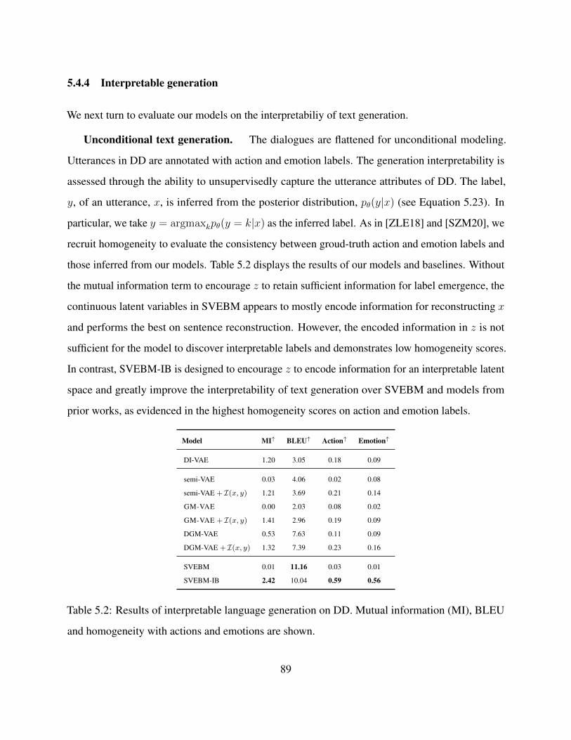
5.4.4 Interpretable generation

We next turn to evaluate our models on the interpretabiliy of text generation.

Unconditional text generation. The dialogues are flattened for unconditional modeling.

Utterances in DD are annotated with action and emotion labels. The generation interpretability is

assessed through the ability to unsupervisedly capture the utterance attributes of DD. The label,

y, of an utterance, x, is inferred from the posterior distribution, pθ(y|x) (see Equation 5.23). In

particular, we take y = argmaxkpθ(y = k|x) as the inferred label. As in [ZLE18] and [SZM20], we

recruit homogeneity to evaluate the consistency between groud-truth action and emotion labels and

those inferred from our models. Table 5.2 displays the results of our models and baselines. Without

the mutual information term to encourage z to retain sufficient information for label emergence, the

continuous latent variables in SVEBM appears to mostly encode information for reconstructing x

and performs the best on sentence reconstruction. However, the encoded information in z is not

sufficient for the model to discover interpretable labels and demonstrates low homogeneity scores.

In contrast, SVEBM-IB is designed to encourage z to encode information for an interpretable latent

space and greatly improve the interpretability of text generation over SVEBM and models from

prior works, as evidenced in the highest homogeneity scores on action and emotion labels.

Model MI↑ BLEU↑ Action↑ Emotion↑

DI-VAE 1.20 3.05 0.18 0.09

semi-VAE 0.03 4.06 0.02 0.08

semi-VAE + I(x, y) 1.21 3.69 0.21 0.14

GM-VAE 0.00 2.03 0.08 0.02

GM-VAE + I(x, y) 1.41 2.96 0.19 0.09

DGM-VAE 0.53 7.63 0.11 0.09

DGM-VAE + I(x, y) 1.32 7.39 0.23 0.16

SVEBM 0.01 11.16 0.03 0.01

SVEBM-IB 2.42 10.04 0.59 0.56

Table 5.2: Results of interpretable language generation on DD. Mutual information (MI), BLEU

and homogeneity with actions and emotions are shown.

89

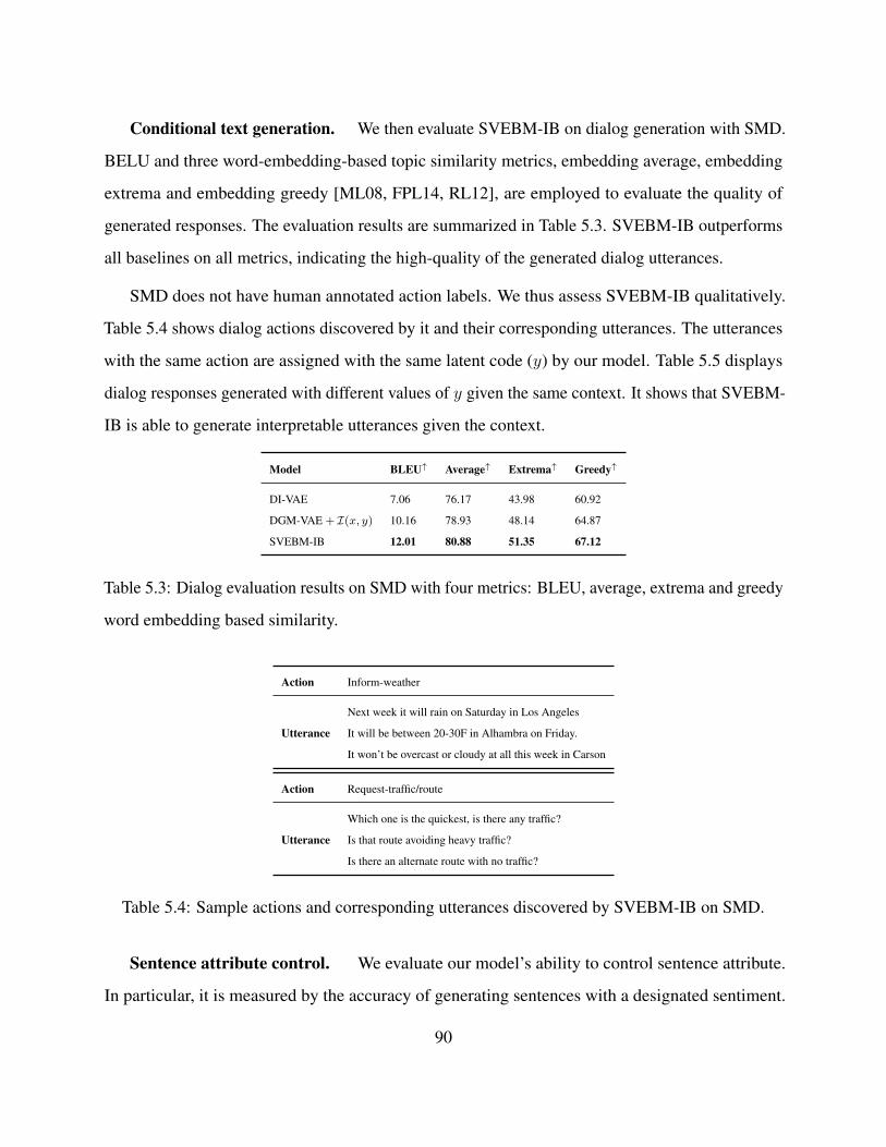
Conditional text generation. We then evaluate SVEBM-IB on dialog generation with SMD.

BELU and three word-embedding-based topic similarity metrics, embedding average, embedding

extrema and embedding greedy [ML08, FPL14, RL12], are employed to evaluate the quality of

generated responses. The evaluation results are summarized in Table 5.3. SVEBM-IB outperforms

all baselines on all metrics, indicating the high-quality of the generated dialog utterances.

SMD does not have human annotated action labels. We thus assess SVEBM-IB qualitatively.

Table 5.4 shows dialog actions discovered by it and their corresponding utterances. The utterances

with the same action are assigned with the same latent code (y) by our model. Table 5.5 displays

dialog responses generated with different values of y given the same context. It shows that SVEBM-

IB is able to generate interpretable utterances given the context.

Model BLEU↑ Average↑ Extrema↑ Greedy↑

DI-VAE 7.06 76.17 43.98 60.92

DGM-VAE + I(x, y) 10.16 78.93 48.14 64.87

SVEBM-IB 12.01 80.88 51.35 67.12

Table 5.3: Dialog evaluation results on SMD with four metrics: BLEU, average, extrema and greedy

word embedding based similarity.

Action Inform-weather

Utterance

Next week it will rain on Saturday in Los Angeles

It will be between 20-30F in Alhambra on Friday.

It won’t be overcast or cloudy at all this week in Carson

Action Request-traffic/route

Utterance

Which one is the quickest, is there any traffic?

Is that route avoiding heavy traffic?

Is there an alternate route with no traffic?

Table 5.4: Sample actions and corresponding utterances discovered by SVEBM-IB on SMD.

Sentence attribute control. We evaluate our model’s ability to control sentence attribute.

In particular, it is measured by the accuracy of generating sentences with a designated sentiment.

90

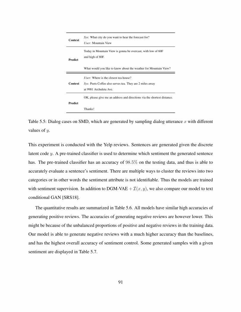
ContextSys: What city do you want to hear the forecast for?

User: Mountain View

Predict

Today in Mountain View is gonna be overcast, with low of 60F

and high of 80F.

What would you like to know about the weather for Mountain View?

Context

User: Where is the closest tea house?

Sys: Peets Coffee also serves tea. They are 2 miles away

at 9981 Archuleta Ave.

Predict

OK, please give me an address and directions via the shortest distance.

Thanks!

Table 5.5: Dialog cases on SMD, which are generated by sampling dialog utterance x with different

values of y.

This experiment is conducted with the Yelp reviews. Sentences are generated given the discrete

latent code y. A pre-trained classifier is used to determine which sentiment the generated sentence

has. The pre-trained classifier has an accuracy of 98.5% on the testing data, and thus is able to

accurately evaluate a sentence’s sentiment. There are multiple ways to cluster the reviews into two

categories or in other words the sentiment attribute is not identifiable. Thus the models are trained

with sentiment supervision. In addition to DGM-VAE + I(x, y), we also compare our model to text

conditional GAN [SRS18].

The quantitative results are summarized in Table 5.6. All models have similar high accuracies of

generating positive reviews. The accuracies of generating negative reviews are however lower. This

might be because of the unbalanced proportions of positive and negative reviews in the training data.

Our model is able to generate negative reviews with a much higher accuracy than the baselines,

and has the highest overall accuracy of sentiment control. Some generated samples with a given

sentiment are displayed in Table 5.7.

91

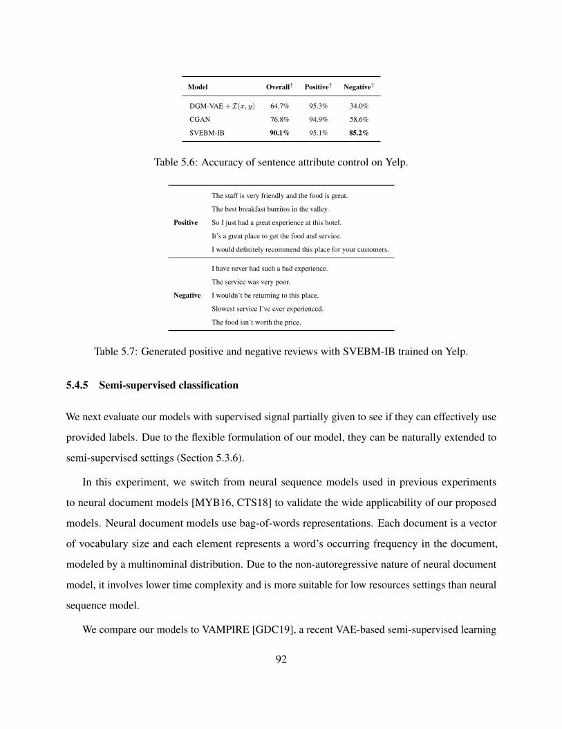
Model Overall↑ Positive↑ Negative↑

DGM-VAE + I(x, y) 64.7% 95.3% 34.0%

CGAN 76.8% 94.9% 58.6%

SVEBM-IB 90.1% 95.1% 85.2%

Table 5.6: Accuracy of sentence attribute control on Yelp.

Positive

The staff is very friendly and the food is great.

The best breakfast burritos in the valley.

So I just had a great experience at this hotel.

It’s a great place to get the food and service.

I would definitely recommend this place for your customers.

Negative

I have never had such a bad experience.

The service was very poor.

I wouldn’t be returning to this place.

Slowest service I’ve ever experienced.

The food isn’t worth the price.

Table 5.7: Generated positive and negative reviews with SVEBM-IB trained on Yelp.

5.4.5 Semi-supervised classification

We next evaluate our models with supervised signal partially given to see if they can effectively use

provided labels. Due to the flexible formulation of our model, they can be naturally extended to

semi-supervised settings (Section 5.3.6).

In this experiment, we switch from neural sequence models used in previous experiments

to neural document models [MYB16, CTS18] to validate the wide applicability of our proposed

models. Neural document models use bag-of-words representations. Each document is a vector

of vocabulary size and each element represents a word’s occurring frequency in the document,

modeled by a multinominal distribution. Due to the non-autoregressive nature of neural document

model, it involves lower time complexity and is more suitable for low resources settings than neural

sequence model.

We compare our models to VAMPIRE [GDC19], a recent VAE-based semi-supervised learning

92

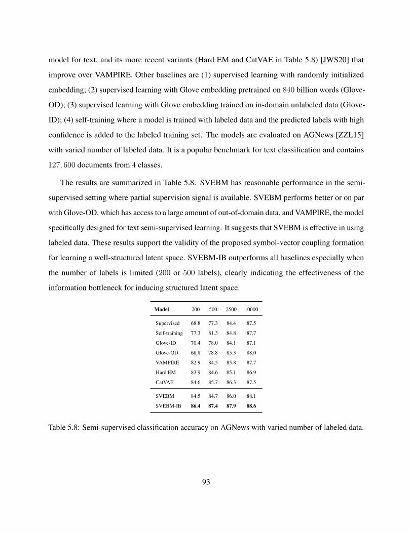
model for text, and its more recent variants (Hard EM and CatVAE in Table 5.8) [JWS20] that

improve over VAMPIRE. Other baselines are (1) supervised learning with randomly initialized

embedding; (2) supervised learning with Glove embedding pretrained on 840 billion words (Glove-

OD); (3) supervised learning with Glove embedding trained on in-domain unlabeled data (Glove-

ID); (4) self-training where a model is trained with labeled data and the predicted labels with high

confidence is added to the labeled training set. The models are evaluated on AGNews [ZZL15]

with varied number of labeled data. It is a popular benchmark for text classification and contains

127, 600 documents from 4 classes.

The results are summarized in Table 5.8. SVEBM has reasonable performance in the semi-

supervised setting where partial supervision signal is available. SVEBM performs better or on par

with Glove-OD, which has access to a large amount of out-of-domain data, and VAMPIRE, the model

specifically designed for text semi-supervised learning. It suggests that SVEBM is effective in using

labeled data. These results support the validity of the proposed symbol-vector coupling formation

for learning a well-structured latent space. SVEBM-IB outperforms all baselines especially when

the number of labels is limited (200 or 500 labels), clearly indicating the effectiveness of the

information bottleneck for inducing structured latent space.

Model 200 500 2500 10000

Supervised 68.8 77.3 84.4 87.5

Self-training 77.3 81.3 84.8 87.7

Glove-ID 70.4 78.0 84.1 87.1

Glove-OD 68.8 78.8 85.3 88.0

VAMPIRE 82.9 84.5 85.8 87.7

Hard EM 83.9 84.6 85.1 86.9

CatVAE 84.6 85.7 86.3 87.5

SVEBM 84.5 84.7 86.0 88.1

SVEBM-IB 86.4 87.4 87.9 88.6

Table 5.8: Semi-supervised classification accuracy on AGNews with varied number of labeled data.

93

5.5 Related work and discussions

Text generation. VAE is a prominent generative model [KW14, RMW14]. It is first applied

to text modeling by [BVV16]. Following works apply VAE to a wide variety of challenging

text generation problems such as dialog generation [SSB16, SSL17, ZZE17, ZLE18], machine

translation [ZXS16], text summarization [LLB17], and paraphrase generation [GAS18]. Also, a

large number of following works have endeavored to improve language modeling and text generation

with VAE by addressing issues like posterior collapse [ZKZ18, LHN19, FLL19, HSN19].

Recently, [ZLE18] and [SZM20] explore the interpretability of text generation with VAEs.

While the model in [ZLE18] has a discrete latent space, in [SZM20] the model contains both

discrete (y) and continuous (z) variables which follow Gaussian mixture. Similarly, we use both

discrete and continuous variables. But they are coupled together through an EBM which is more

expressive than Gaussian mixture as a prior model, as illustrated in our experiments where both

SVEBM and SVEBM-IB outperform the models from [SZM20] on language modeling and text

generation. Moreover, our coupling formulation makes the mutual information between z and y can

be easily computed without the need to train and tune an additional auxiliary inference network

for y or deal with the non-diffierentibility with regard to it, while [SZM20] recruits an auxiliary

network to infer y conditional on x to compute their mutual information 2. [KMR14] also proposes

a VAE with both discrete and continuous latent variables but they are independent and z follows an

non-informative prior. These designs make it less powerful than ours in both generation quality and

interpretability as evidenced in our experiments.

Energy-based model. Recent works [XLZ16, NHZ19, HNZ20b] demonstrate the effective-

ness of EBMs in modeling complex dependency. [PHN20] proposes to learn an EBM in the latent

space as a prior model for the continuous latent vector, which greatly improves the model expres-

sivity and demonstrates strong performance on text, image, molecule generation, and trajectory

2Unlike our model which maximizes the mutual information between z and y following the information bottleneckprinciple [TPB00], they maximizes the mutual information between the observed data x and the label y.

94

generation [PHW20, PZX21]. We also recruit an EBM as the prior model but this EBM couples a

continuous vector and a discrete one, allowing for learning a more structured latent space, rendering

generation interpretable, and admitting classification. In addition, the prior work uses MCMC for

posterior inference but we recruits an inference network, qϕ(z|x), so that we can efficiently optimize

over it, which is necessary for learning with the information bottleneck principle. Thus, this design

admits a natural extension based on information bottleneck.

[GWJ19] proposes the joint energy-based model (JEM) which is a classifier based EBM. Our

model moves JEM to latent space. This brings two benefits. (1) Learning EBM in the data space

usually involves expensive MCMC sampling. Our EBM is built in the latent space which has a

much lower dimension and thus the sampling is much faster and has better mixing. (2) It is not

straightforward to apply JEM to text data since it uses gradient-based sampling while the data space

of text is non-differentiable.

Information bottleneck. Information bottleneck proposed by [TPB00] is an appealing

principle to find good representations that trade-offs between the minimality of the representation

and its sufficiency for predicting labels. Computing mutual information involved in applying

this principle is however often computationally challenging. [AFD16] proposes a variational

approach to reduce the computation complexity and uses it train supervised classifiers. In contrast,

the information bottleneck in our model is embedded in a generative model and learned in an

unsupervised manner.

5.6 Conclusion

In this work, we formulate a latent space EBM which couples a dense vector for generation and a

symbolic vector for interpretability and classification. The symbol or category can be inferred from

the observed example based on the dense vector. The latent space EBM is used as the prior model

for text generation model. The symbol-vector coupling, the generator network, and the inference

network are learned jointly by maximizing the variational lower bound of the log-likelihood.

95

Our model can be learned in unsupervised setting and the learning can be naturally extended to

semi-supervised setting. The coupling formulation and the variational learning together naturally

admit an incorporation of information bottleneck which encourages the continuous latent vector to

extract information from the observed example that is informative of the underlying symbol. Our

experiments demonstrate that the proposed model learns a well-structured and meaningful latent

space, which (1) guides the top-down generator to generate text with high quality and interpretability,

and (2) can be leveraged to effectively and accurately classify text.

96

CHAPTER 6

Conclusion

Driven by the power of modern neural networks and computation, machine learning has achieved

great progress in many areas. Also, numerous models and learning algorithms have been developed.

Following the principle of probabilistic modeling and maximum likelihood learning, we seek a

simple but versatile model with principled learning algorithm which enables a variety of applications

in modeling data and patterns of high-dimensionality and complexity. It is also our hope that a

simple and principled model would pave the way towards future research through easy adaption and

extension.

To achieve such a goal, we propose a unification of three probabilistic models that are widely

used to model complex patterns: generator model, EBM, and discriminative model. The unification

first starts with an integration of generator model and EBM (Chapter 2). Comparing these two

models, EBM is expressive but poses challenges in sampling, while generator model is relatively

less expressive but convenient and efficient in terms of sampling. The unification is achieved by

learning an EBM in the latent space as the prior distribution of the generator model, resulting in the

foundation of this dissertation, latent space energy-based model. Due to the low dimensionality

of the latent space, a simple energy function in latent space can capture regularities in the data

effectively. Thus, latent space EBM is much more expressive than the original generator model with

little cost in terms of model complexity and computational complexity. Also, MCMC sampling in

latent space is much more efficient and mixes better than that in the observed data space since the

energy function defined in the data space has to be highly multi-modal in order to fit the usually

multi-modal data distribution. The model can be learned by maximum likelihood, which involves

97

short-run MCMC sampling from both the prior and posterior distributions of the latent vector. The

MCMC sampling can also be amortized by a synthesis network and an inference network. We

formulate the learning algorithm as a perturbation of maximum likelihood learning in terms of both

objective function and estimating equation, so that the learning algorithm has a solid theoretical

foundation.

To empirically verify the proposed model and learning algorithm, we conduct extensively

experiments on natural images and text such as human faces, financial news. Our experiments

show that the model can effectively learn from these high-dimensional and complex datasets. The

well-learned model enables us to sample faithful and diverse samples of natural images and text.

Moreover, given the good fit, the posterior of the latent vector can separate probability densities for

normal and anomalous data, making this model a natural tool for anomaly detection.

We next apply the established latent space EBM in two scenarios, which exploit two respective

aspects of the model. In one application (Chapter 3), we leverage the expressiveness of latent

space EBM and use it model molecules when they are represented in SMILES, a simple format

of linear strings. Despite SMILES’ convenience, models relying on this simple representation

tend to generate invalid samples and duplicates. Owing to its expressiveness, learned latent space

EBM on molecules in this simple and convenient representation is able to generate molecules

with high validity, diversity and uniqueness, and generated molecules have chemical properties

whose distributions almost perfectly match those of the real molecules. These results provide

strong evidence that the proposed model is able to automatically learn complicated chemical rules

implicitly from the data. Accurately modeling the observed distribution of molecules is the first

and key step towards molecule design for drug discovery and material science. The next step is

to generate molecules with desirable properties such as high octanol/water partition coefficient

(logP) (which measures solubility) and high drug-likeness (QED). To this end, a natural extension of

our model, pα(z)pβ(x|z)pγ(y|z), can be used, where y indicates the value of chemical property of

interest, which is often easy to obtain via open-sourced software like Rdkit [Lan01]. This model can

be learned jointly with an algorithm similar to the one developed in Chapter 2 on a dataset {(x, y)}.

98

We can then do controlled generation by sampling from pθ(z|y) ∝ pα(z)pγ(y|z). Molecules with

high y can obtained by gradually increasing y and several iterative rounds of training.

In another application (Chapter 4), we explore the aspect of EBM as a cost function and make

a connection with inverse reinforcement learning for diverse human trajectory forecast. The cost

function is learned from expert demonstrations projected into the latent space. To make a forecast,

optimizing the cost function leads to a belief vector, which is then project to the trajectory space by

a policy network. The proposed model is able to make accurate, multi-modal, and social compliant

trajectory predictions. Besides human trajectory forecasting, we can also apply this model or some

variants to other planning or control problems. Also, due to the top-level latent variable z which can

be considered a latent plan, our model goes beyond the scope of Markov decision process. This is

an interesting and a fruitful aspect of latent space EBM which shall be investigated in future work.

Building on top of the unification of generator model and EBM, we further integrate the

discriminative model into our model (Chapter 5). In this integration, the energy term of the prior

model couples a continuous latent vector and a symbolic one-hot vector, so that discrete category

can be inferred from the observed example based on the continuous latent vector. Such a latent space

coupling naturally enables incorporation of information bottleneck regularization to encourage the

continuous latent vector to extract information from the observed example that is informative of the

underlying category. In contrast to the classical information bottleneck developed for the analysis of

supervised learning, our learning objective is an information bottleneck for unsupervised learning.

In our experiments, we find that the symbol-vector coupling with information bottleneck leads to

a well-structured latent space such that the generator model generates text with high quality and

interpretability and it serves as a high-performing classifier with a limited amount of labeled data.

99

REFERENCES

[ACB17] Martın Arjovsky, Soumith Chintala, and Leon Bottou. “Wasserstein Generative Adver-sarial Networks.” In Proceedings of the 34th International Conference on MachineLearning, ICML 2017, Sydney, NSW, Australia, 6-11 August 2017, pp. 214–223, 2017.

[AFD16] Alexander A Alemi, Ian Fischer, Joshua V Dillon, and Kevin Murphy. “Deep varia-tional information bottleneck.” arXiv preprint arXiv:1612.00410, 2016.

[AGR16] Alexandre Alahi, Kratarth Goel, Vignesh Ramanathan, Alexandre Robicquet, Li Fei-Fei, and Silvio Savarese. “Social lstm: Human trajectory prediction in crowded spaces.”In Proceedings of the IEEE conference on computer vision and pattern recognition, pp.961–971, 2016.

[AHS85] David H. Ackley, Geoffrey E. Hinton, and Terrence J. Sejnowski. “A LearningAlgorithm for Boltzmann Machines.” Cognitive Science, 9(1):147–169, 1985.

[ASK20] Jyoti Aneja, Alexander Schwing, Jan Kautz, and Arash Vahdat. “NCP-VAE: Varia-tional Autoencoders with Noise Contrastive Priors.”, 2020.

[BAP15] Samuel R. Bowman, Gabor Angeli, Christopher Potts, and Christopher D. Manning. “Alarge annotated corpus for learning natural language inference.” In Proceedings of the2015 Conference on Empirical Methods in Natural Language Processing, pp. 632–642,Lisbon, Portugal, September 2015. Association for Computational Linguistics.

[BDD93] Peter F Brown, Stephen A Della Pietra, Vincent J Della Pietra, and Robert L Mercer.“The mathematics of statistical machine translation: Parameter estimation.” Computa-tional linguistics, 19(2):263–311, 1993.

[BDS18] Andrew Brock, Jeff Donahue, and Karen Simonyan. “Large scale gan training for highfidelity natural image synthesis.” arXiv preprint arXiv:1809.11096, 2018.

[BGS15] Yuri Burda, Roger Grosse, and Ruslan Salakhutdinov. “Importance weighted autoen-coders.” arXiv preprint arXiv:1509.00519, 2015.

[BHF19] Apratim Bhattacharyya, Michael Hanselmann, Mario Fritz, Bernt Schiele, andChristoph-Nikolas Straehle. “Conditional flow variational autoencoders for struc-tured sequence prediction.” arXiv preprint arXiv:1908.09008, 2019.

[BHL16] M. Bahram, C. Hubmann, A. Lawitzky, M. Aeberhard, and D. Wollherr. “A combinedmodel and learning based framework for interaction-aware maneuver prediction.” IEEETransactions on Intelligent Transportation Systems, 2016.

[BM19] Matthias Bauer and Andriy Mnih. “Resampled Priors for Variational Autoencoders.”In The 22nd International Conference on Artificial Intelligence and Statistics, pp.66–75, 2019.

100

[BMD13] Yoshua Bengio, Gregoire Mesnil, Yann Dauphin, and Salah Rifai. “Better mixing viadeep representations.” In International conference on machine learning, pp. 552–560,2013.

[BMR20] Tom B Brown, Benjamin Mann, Nick Ryder, Melanie Subbiah, Jared Kaplan, PrafullaDhariwal, Arvind Neelakantan, Pranav Shyam, Girish Sastry, Amanda Askell, et al.“Language models are few-shot learners.” arXiv preprint arXiv:2005.14165, 2020.

[BVV16] Samuel R. Bowman, Luke Vilnis, Oriol Vinyals, Andrew Dai, Rafal Jozefowicz, andSamy Bengio. “Generating Sentences from a Continuous Space.” In Proceedingsof The 20th SIGNLL Conference on Computational Natural Language Learning, pp.10–21, Berlin, Germany, August 2016. Association for Computational Linguistics.

[CMG14] Kyunghyun Cho, Bart van Merrienboer, Caglar Gulcehre, Dzmitry Bahdanau, FethiBougares, Holger Schwenk, and Yoshua Bengio. “Learning Phrase Representationsusing RNN Encoder–Decoder for Statistical Machine Translation.” In Proceedings ofthe 2014 Conference on Empirical Methods in Natural Language Processing (EMNLP),pp. 1724–1734, 2014.

[CSA18] Ondrej Cıfka, Aliaksei Severyn, Enrique Alfonseca, and Katja Filippova. “Eval all,trust a few, do wrong to none: Comparing sentence generation models.” arXiv preprintarXiv:1804.07972, 2018.

[CT06] Thomas M. Cover and Joy A. Thomas. Elements of information theory (2. ed.). Wiley,2006.

[CTS18] Dallas Card, Chenhao Tan, and Noah A Smith. “Neural Models for Documentswith Metadata.” In Proceedings of the 56th Annual Meeting of the Association forComputational Linguistics (Volume 1: Long Papers), pp. 2031–2040, 2018.

[DAB17] Zihang Dai, Amjad Almahairi, Philip Bachman, Eduard H. Hovy, and Aaron C.Courville. “Calibrating Energy-based Generative Adversarial Networks.” In 5thInternational Conference on Learning Representations, ICLR 2017, Toulon, France,April 24-26, 2017, Conference Track Proceedings, 2017.

[DCL18] Jacob Devlin, Ming-Wei Chang, Kenton Lee, and Kristina Toutanova. “Bert: Pre-training of deep bidirectional transformers for language understanding.” arXiv preprintarXiv:1810.04805, 2018.

[DLR77] Arthur P Dempster, Nan M Laird, and Donald B Rubin. “Maximum likelihood fromincomplete data via the EM algorithm.” Journal of the Royal Statistical Society: SeriesB (Methodological), 39(1):1–22, 1977.

[DLW15] Jifeng Dai, Yang Lu, and Ying Nian Wu. “Generative Modeling of ConvolutionalNeural Networks.” In 3rd International Conference on Learning Representations,

101

ICLR 2015, San Diego, CA, USA, May 7-9, 2015, Conference Track Proceedings,2015.

[DM14] Kingma Diederik and Welling Max. “Auto-Encoding Variational Bayes.” In ICLR.2014.

[DM19] Yilun Du and Igor Mordatch. “Implicit Generation and Generalization in Energy-BasedModels.” CoRR, abs/1903.08689, 2019.

[DMD20] Isht Dwivedi, Srikanth Malla, Behzad Dariush, and Chiho Choi. “SSP: Single Shot Fu-ture Trajectory Prediction.” In Proceedings of the IEEE/RSJ International Conferenceon Intelligent Robots and Systems (IROS), 2020.

[DRT18] N. Deo, A. Rangesh, and M. M. Trivedi. “How would surround vehicles move? a uni-fied framework for maneuver classification and motion prediction.” arXiv:1801.06523,2018.

[DSB17] Laurent Dinh, Jascha Sohl-Dickstein, and Samy Bengio. “Density estimation usingReal NVP.” In 5th International Conference on Learning Representations, ICLR 2017,Toulon, France, April 24-26, 2017, Conference Track Proceedings, 2017.

[DT18a] Nachiket Deo and Mohan M. Trivedi. “Convolutional Social Pooling for VehicleTrajectory Prediction.” In IEEE Computer Vision and Pattern Recognition Workshopon Joint Detection, Tracking, and Prediction in the Wild, 2018.

[DT18b] Nachiket Deo and Mohan M. Trivedi. “Multi-Modal Trajectory Prediction of Surround-ing Vehicles with Maneuver based LSTMs.” In IEEE Intelligent Vehicles Symposium(IV), 2018.

[DT20] Nachiket Deo and Mohan M Trivedi. “Trajectory forecasts in unknown environmentsconditioned on grid-based plans.” arXiv preprint arXiv:2001.00735, 2020.

[DW19a] Bin Dai and David Wipf. “Diagnosing and Enhancing VAE Models.” In InternationalConference on Learning Representations, 2019.

[DW19b] Bin Dai and David Wipf. “Diagnosing and enhancing vae models.” arXiv preprintarXiv:1903.05789, 2019.

[EKC17] Mihail Eric, Lakshmi Krishnan, Francois Charette, and Christopher D Manning. “Key-Value Retrieval Networks for Task-Oriented Dialogue.” Annual Meeting of the SpecialInterest Group on Discourse and Dialogue, pp. 37–49, 2017.

[FCA16] Chelsea Finn, Paul F. Christiano, Pieter Abbeel, and Sergey Levine. “A Connectionbetween Generative Adversarial Networks, Inverse Reinforcement Learning, andEnergy-Based Models.” CoRR, abs/1611.03852, 2016.

102

[FLA16] Chelsea Finn, Sergey Levine, and Pieter Abbeel. “Guided cost learning: Deep inverseoptimal control via policy optimization.” In International conference on machinelearning, pp. 49–58, 2016.

[FLL19] Hao Fu, Chunyuan Li, Xiaodong Liu, Jianfeng Gao, Asli Celikyilmaz, and LawrenceCarin. “Cyclical Annealing Schedule: A Simple Approach to Mitigating KL Van-ishing.” In Proceedings of the 2019 Conference of the North American Chapter ofthe Association for Computational Linguistics: Human Language Technologies, Vol-ume 1 (Long and Short Papers), pp. 240–250, Minneapolis, Minnesota, June 2019.Association for Computational Linguistics.

[FPL14] Gabriel Forgues, Joelle Pineau, Jean-Marie Larcheveque, and Real Tremblay. “Boot-strapping dialog systems with word embeddings.” In NIPS, Modern Machine Learningand Natural Language Processing Workshop, volume 2, 2014.

[GAS18] Ankush Gupta, Arvind Agarwal, Prawaan Singh, and Piyush Rai. “A deep generativeframework for paraphrase generation.” In Proceedings of the AAAI Conference onArtificial Intelligence, volume 32, 2018.

[GB10] Xavier Glorot and Yoshua Bengio. “Understanding the difficulty of training deep feed-forward neural networks.” In Proceedings of the thirteenth international conferenceon artificial intelligence and statistics, pp. 249–256, 2010.

[GDC19] Suchin Gururangan, Tam Dang, Dallas Card, and Noah A Smith. “Variational Pre-training for Semi-supervised Text Classification.” In Proceedings of the 57th AnnualMeeting of the Association for Computational Linguistics, pp. 5880–5894, 2019.

[GG15] Yarin Gal and Zoubin Ghahramani. “Bayesian convolutional neural networks withBernoulli approximate variational inference.” arXiv preprint arXiv:1506.02158, 2015.

[GG16] Yarin Gal and Zoubin Ghahramani. “Dropout as a bayesian approximation: Repre-senting model uncertainty in deep learning.” In international conference on machinelearning, pp. 1050–1059. PMLR, 2016.

[GH10] Michael Gutmann and Aapo Hyvarinen. “Noise-contrastive estimation: A new estima-tion principle for unnormalized statistical models.” In Proceedings of the ThirteenthInternational Conference on Artificial Intelligence and Statistics, AISTATS 2010, ChiaLaguna Resort, Sardinia, Italy, May 13-15, 2010, pp. 297–304, 2010.

[GHC20] Francesco Giuliari, Irtiza Hasan, Marco Cristani, and Fabio Galasso. “TransformerNetworks for Trajectory Forecasting.”, 2020.

[GJF18] Agrim Gupta, Justin Johnson, Li Fei-Fei, Silvio Savarese, and Alexandre Alahi. “So-cial gan: Socially acceptable trajectories with generative adversarial networks.” InProceedings of the IEEE Conference on Computer Vision and Pattern Recognition, pp.2255–2264, 2018.

103

[GLZ18] Ruiqi Gao, Yang Lu, Junpei Zhou, Song-Chun Zhu, and Ying Nian Wu. “LearningGenerative ConvNets via Multi-Grid Modeling and Sampling.” In 2018 IEEE Confer-ence on Computer Vision and Pattern Recognition, CVPR 2018, Salt Lake City, UT,USA, June 18-22, 2018, pp. 9155–9164, 2018.

[GNK20] Ruiqi Gao, Erik Nijkamp, Diederik P Kingma, Zhen Xu, Andrew M Dai, and Ying NianWu. “Flow contrastive estimation of energy-based models.” In Proceedings of theIEEE/CVF Conference on Computer Vision and Pattern Recognition, pp. 7518–7528,2020.

[GPM14a] I. Goodfellow, J. Pouget-Abadie, M. Mirza, B. Xu, D. Warde-Farley, S. Ozair,A. Courville, and Y. Bengio. “Generative adversarial nets.” In Advances in neu-ral information processing systems, pp. 2672–2680. 2014.

[GPM14b] Ian J. Goodfellow, Jean Pouget-Abadie, Mehdi Mirza, Bing Xu, David Warde-Farley,Sherjil Ozair, Aaron C. Courville, and Yoshua Bengio. “Generative Adversarial Nets.”In Advances in Neural Information Processing Systems 27: Annual Conference onNeural Information Processing Systems 2014, December 8-13 2014, Montreal, Quebec,Canada, pp. 2672–2680, 2014.

[GSV20] Partha Ghosh, Mehdi S. M. Sajjadi, Antonio Vergari, Michael Black, and BernhardScholkopf. “From Variational to Deterministic Autoencoders.” In InternationalConference on Learning Representations, 2020.

[GWD18] Rafael Gomez-Bombarelli, Jennifer N Wei, David Duvenaud, Jose Miguel Hernandez-Lobato, Benjamın Sanchez-Lengeling, Dennis Sheberla, Jorge Aguilera-Iparraguirre,Timothy D Hirzel, Ryan P Adams, and Alan Aspuru-Guzik. “Automatic chemicaldesign using a data-driven continuous representation of molecules.” ACS centralscience, 4(2):268–276, 2018.

[GWJ19] Will Grathwohl, Kuan-Chieh Wang, Joern-Henrik Jacobsen, David Duvenaud, Mo-hammad Norouzi, and Kevin Swersky. “Your classifier is secretly an energy basedmodel and you should treat it like one.” In International Conference on LearningRepresentations, 2019.

[GZW03] Cheng-En Guo, Song-Chun Zhu, and Ying Nian Wu. “Modeling visual patterns byintegrating descriptive and generative methods.” International Journal of ComputerVision, 53(1):5–29, 2003.

[HDF95] Geoffrey E Hinton, Peter Dayan, Brendan J Frey, and Radford M Neal. “The” wake-sleep” algorithm for unsupervised neural networks.” Science, 268(5214):1158–1161,1995.

[Hin02] Geoffrey E. Hinton. “Training Products of Experts by Minimizing Contrastive Diver-gence.” Neural Computation, 14(8):1771–1800, 2002.

104

[HKO04] Aapo Hyvarinen, Juha Karhunen, and Erkki Oja. Independent component analysis.John Wiley & Sons, 2004.

[HLZ17] Tian Han, Yang Lu, Song-Chun Zhu, and Ying Nian Wu. “Alternating Back-Propagation for Generator Network.” In Proceedings of the Thirty-First AAAI Confer-ence on Artificial Intelligence, February 4-9, 2017, San Francisco, California, USA.,pp. 1976–1984, 2017.

[HM95] D. Helbing and P. Molnar. “Social force model for pedestrian dynamics.” Physicalreview E, 51(5):4282, 1995.

[HNF19a] Tian Han, Erik Nijkamp, Xiaolin Fang, Mitch Hill, Song-Chun Zhu, and Ying NianWu. “Divergence triangle for joint training of generator model, energy-based model,and inferential model.” In Proceedings of the IEEE Conference on Computer Visionand Pattern Recognition, pp. 8670–8679, 2019.

[HNF19b] Tian Han, Erik Nijkamp, Xiaolin Fang, Mitch Hill, Song-Chun Zhu, and Ying Nian Wu.“Divergence Triangle for Joint Training of Generator Model, Energy-Based Model, andInferential Model.” In IEEE Conference on Computer Vision and Pattern Recognition,CVPR 2019, Long Beach, CA, USA, June 16-20, 2019, pp. 8670–8679, 2019.

[HNZ20a] Tian Han, Erik Nijkamp, Linqi Zhou, Bo Pang, Song-Chun Zhu, and Ying NianWu. “Joint Training of Variational Auto-Encoder and Latent Energy-Based Model.” InProceedings of the IEEE/CVF Conference on Computer Vision and Pattern Recognition,pp. 7978–7987, 2020.

[HNZ20b] Tian Han, Erik Nijkamp, Linqi Zhou, Bo Pang, Song-Chun Zhu, and Ying Nian Wu.“Joint Training of Variational Auto-Encoder and Latent Energy-Based Model.” In TheIEEE/CVF Conference on Computer Vision and Pattern Recognition (CVPR), June2020.

[Hof17] Matthew D Hoffman. “Learning deep latent Gaussian models with Markov chainMonte Carlo.” In International conference on machine learning, pp. 1510–1519, 2017.

[HOT06] Geoffrey E. Hinton, Simon Osindero, and Yee Whye Teh. “A Fast Learning Algorithmfor Deep Belief Nets.” Neural Computation, 18(7):1527–1554, 2006.

[HPW21] Wenjuan Han, Bo Pang, and Ying Nian Wu. “Robust Transfer Learning with PretrainedLanguage Models through Adapters.” In Proceedings of the 59th Annual Meeting of theAssociation for Computational Linguistics and the 11th International Joint Conferenceon Natural Language Processing (Volume 2: Short Papers), pp. 854–861, 2021.

[HS97] Sepp Hochreiter and Jurgen Schmidhuber. “Long short-term memory.” Neural compu-tation, 9(8):1735–1780, 1997.

105

[HSN19] Junxian He, Daniel Spokoyny, Graham Neubig, and Taylor Berg-Kirkpatrick. “Lag-ging Inference Networks and Posterior Collapse in Variational Autoencoders.” InProceedings of ICLR, 2019.

[HST18] Irtiza Hasan, Francesco Setti, Theodore Tsesmelis, Alessio Del Bue, Fabio Galasso,and Marco Cristani. “MX-LSTM: mixing tracklets and vislets to jointly forecasttrajectories and head poses.” Proceedings of the IEEE International Conference onComputer Vision and Pattern Recognition, 2018.

[HTA17] Tuomas Haarnoja, Haoran Tang, Pieter Abbeel, and Sergey Levine. “Reinforcementlearning with deep energy-based policies.” In International Conference on MachineLearning, pp. 1352–1361. PMLR, 2017.

[HZR16] Kaiming He, Xiangyu Zhang, Shaoqing Ren, and Jian Sun. “Deep residual learningfor image recognition.” In Proceedings of the IEEE conference on computer visionand pattern recognition, pp. 770–778, 2016.

[IP19] Boris Ivanovic and Marco Pavone. “The trajectron: Probabilistic multi-agent trajectorymodeling with dynamic spatiotemporal graphs.” In Proceedings of the IEEE/CVFInternational Conference on Computer Vision, pp. 2375–2384, 2019.

[ISM12] John J Irwin, Teague Sterling, Michael M Mysinger, Erin S Bolstad, and Ryan GColeman. “ZINC: a free tool to discover chemistry for biology.” Journal of chemicalinformation and modeling, 52(7):1757–1768, 2012.

[JLT17] Long Jin, Justin Lazarow, and Zhuowen Tu. “Introspective Classification with Con-volutional Nets.” In Advances in Neural Information Processing Systems 30: AnnualConference on Neural Information Processing Systems 2017, 4-9 December 2017,Long Beach, CA, USA, pp. 823–833, 2017.

[JWS20] Shuning Jin, Sam Wiseman, Karl Stratos, and Karen Livescu. “Discrete Latent VariableRepresentations for Low-Resource Text Classification.” In Proceedings of the 58thAnnual Meeting of the Association for Computational Linguistics, pp. 4831–4842,Online, July 2020. Association for Computational Linguistics.

[KB15] Diederik P. Kingma and Jimmy Ba. “Adam: A Method for Stochastic Optimization.”In 3rd International Conference on Learning Representations, ICLR 2015, San Diego,CA, USA, May 7-9, 2015, Conference Track Proceedings, 2015.

[KGC19] Rithesh Kumar, Anirudh Goyal, Aaron C. Courville, and Yoshua Bengio. “MaximumEntropy Generators for Energy-Based Models.” CoRR, abs/1901.08508, 2019.

[KMR14] Durk P Kingma, Shakir Mohamed, Danilo Jimenez Rezende, and Max Welling. “Semi-supervised learning with deep generative models.” In Advances in neural informationprocessing systems, pp. 3581–3589, 2014.

106

[KMW17] A. Kuefler, J. Morton, T. Wheeler, and M. Kochenderfer. “Imitating driver behaviorwith generative adversarial networks.” Intelligent Vehicles Symposium (IV), 2017.

[KNH] Alex Krizhevsky, Vinod Nair, and Geoffrey Hinton. “CIFAR-10 (Canadian Institutefor Advanced Research).”.

[KPH17] Matt J Kusner, Brooks Paige, and Jose Miguel Hernandez-Lobato. “Grammar Vari-ational Autoencoder.” In International Conference on Machine Learning, pp. 1945–1954, 2017.

[KSH12] Alex Krizhevsky, Ilya Sutskever, and Geoffrey E Hinton. “ImageNet Classificationwith Deep Convolutional Neural Networks.” In F. Pereira, C. J. C. Burges, L. Bottou,and K. Q. Weinberger, editors, Advances in Neural Information Processing Systems,volume 25. Curran Associates, Inc., 2012.

[KSM19] Vineet Kosaraju, Amir Sadeghian, Roberto Martın-Martın, Ian Reid, S HamidRezatofighi, and Silvio Savarese. “Social-BiGAT: Multimodal Trajectory Forecastingusing Bicycle-GAN and Graph Attention Networks.” arXiv preprint arXiv:1907.03395,2019.

[KW14] Diederik P. Kingma and Max Welling. “Auto-Encoding Variational Bayes.” In 2ndInternational Conference on Learning Representations, ICLR 2014, Banff, AB, Canada,April 14-16, 2014, Conference Track Proceedings, 2014.

[KWM18] Yoon Kim, Sam Wiseman, Andrew Miller, David Sontag, and Alexander Rush. “Semi-Amortized Variational Autoencoders.” In International Conference on Machine Learn-ing, pp. 2678–2687, 2018.

[LAB18] Qi Liu, Miltiadis Allamanis, Marc Brockschmidt, and Alexander Gaunt. “Constrainedgraph variational autoencoders for molecule design.” In Advances in neural informa-tion processing systems, pp. 7795–7804, 2018.

[Lan01] G Landrum. “RDKit: Open-source cheminformatics.”, 201.

[LBH15] Yann LeCun, Yoshua Bengio, and Geoffrey Hinton. “Deep learning.” nature,521(7553):436–444, 2015.

[LCV17] Namhoon Lee, Wongun Choi, Paul Vernaza, Christopher B Choy, Philip HS Torr, andManmohan Chandraker. “DESIRE: Distant future prediction in dynamic scenes withinteracting agents.” In Proceedings of the IEEE Conference on Computer Vision andPattern Recognition, pp. 336–345, 2017.

[LGR09] Honglak Lee, Roger B. Grosse, Rajesh Ranganath, and Andrew Y. Ng. “Convolutionaldeep belief networks for scalable unsupervised learning of hierarchical representations.”In Proceedings of the 26th Annual International Conference on Machine Learning,ICML 2009, Montreal, Quebec, Canada, June 14-18, 2009, pp. 609–616, 2009.

107

[LHN19] Bohan Li, Junxian He, Graham Neubig, Taylor Berg-Kirkpatrick, and Yiming Yang.“A Surprisingly Effective Fix for Deep Latent Variable Modeling of Text.” In Pro-ceedings of the 2019 Conference on Empirical Methods in Natural Language Pro-cessing and the 9th International Joint Conference on Natural Language Processing(EMNLP-IJCNLP), pp. 3603–3614, Hong Kong, China, November 2019. Associationfor Computational Linguistics.

[LJH18] Juncen Li, Robin Jia, He He, and Percy Liang. “Delete, Retrieve, Generate: a SimpleApproach to Sentiment and Style Transfer.” In Proceedings of the 2018 Conferenceof the North American Chapter of the Association for Computational Linguistics:Human Language Technologies, Volume 1 (Long Papers), pp. 1865–1874, New Orleans,Louisiana, June 2018. Association for Computational Linguistics.

[LJH20] Junwei Liang, Lu Jiang, and Alexander Hauptmann. “SimAug: Learning RobustRepresentations from Simulation for Trajectory Prediction.” 2020.

[LJM20] Junwei Liang, Lu Jiang, Kevin Murphy, Ting Yu, and Alexander Hauptmann. “TheGarden of Forking Paths: Towards Multi-Future Trajectory Prediction.” In Proceedingsof the IEEE Conference on Computer Vision and Pattern Recognition, 2020.

[LJN19] Junwei Liang, Lu Jiang, Juan Carlos Niebles, Alexander G Hauptmann, and Li Fei-Fei.“Peeking into the future: Predicting future person activities and locations in videos.” InProceedings of the IEEE Conference on Computer Vision and Pattern Recognition, pp.5725–5734, 2019.

[LJT17] Justin Lazarow, Long Jin, and Zhuowen Tu. “Introspective Neural Networks forGenerative Modeling.” In IEEE International Conference on Computer Vision, ICCV2017, Venice, Italy, October 22-29, 2017, pp. 2793–2802, 2017.

[LKM17] Mario Lucic, Karol Kurach, Marcin Michalski, Sylvain Gelly, and Olivier Bousquet.“Are gans created equal? a large-scale study.” arXiv preprint arXiv:1711.10337, 2017.

[LLB17] Piji Li, Wai Lam, Lidong Bing, and Zihao Wang. “Deep Recurrent Generative Decoderfor Abstractive Text Summarization.” In Proceedings of the 2017 Conference onEmpirical Methods in Natural Language Processing, pp. 2091–2100, 2017.

[LLW15] Ziwei Liu, Ping Luo, Xiaogang Wang, and Xiaoou Tang. “Deep Learning FaceAttributes in the Wild.” In Proceedings of International Conference on ComputerVision (ICCV), 2015.

[LMT19] Jiachen Li, Hengbo Ma, and Masayoshi Tomizuka. “Conditional generative neuralsystem for probabilistic trajectory prediction.” arXiv preprint arXiv:1905.01631, 2019.

[LS01] Daniel D Lee and H Sebastian Seung. “Algorithms for non-negative matrix factoriza-tion.” In Advances in neural information processing systems, pp. 556–562, 2001.

108

[LSS17] Yanran Li, Hui Su, Xiaoyu Shen, Wenjie Li, Ziqiang Cao, and Shuzi Niu. “DailyDialog:A Manually Labelled Multi-turn Dialogue Dataset.” International Joint Conference onNatural Language Processing, 1:986–995, 2017.

[LYT20] Jiachen Li, Fan Yang, Masayoshi Tomizuka, and Chiho Choi. “EvolveGraph: Multi-Agent Trajectory Prediction with Dynamic Relational Reasoning.” In Proceedings ofthe Neural Information Processing Systems (NeurIPS), 2020.

[LZW16] Yang Lu, Song-Chun Zhu, and Ying Nian Wu. “Learning FRAME Models Using CNNFilters.” In Proceedings of the Thirtieth AAAI Conference on Artificial Intelligence,February 12-17, 2016, Phoenix, Arizona, USA, pp. 1902–1910, 2016.

[MGA20] Karttikeya Mangalam, Harshayu Girase, Shreyas Agarwal, Kuan-Hui Lee, EhsanAdeli, Jitendra Malik, and Adrien Gaidon. “It Is Not the Journey but the Destination:Endpoint Conditioned Trajectory Prediction.” arXiv preprint arXiv:2004.02025, 2020.

[MHL17] Wei-Chiu Ma, De-An Huang, Namhoon Lee, and Kris M. Kitani. “ForecastingInteractive Dynamics of Pedestrians with Fictitious Play.” In Proceedings of theIEEE Conference on Computer Vision and Pattern Recognition, pp. 4636–4644. IEEEComputer Society, 2017.

[MKB10] Tomas Mikolov, Martin Karafiat, Lukas Burget, Jan Cernocky, and Sanjeev Khudanpur.“Recurrent neural network based language model.” In Eleventh annual conference ofthe international speech communication association, 2010.

[MKS18] Stephen Merity, Nitish Shirish Keskar, and Richard Socher. “Regularizing and Opti-mizing LSTM Language Models.” In International Conference on Learning Represen-tations, 2018.

[ML08] Jeff Mitchell and Mirella Lapata. “Vector-based models of semantic composition.”proceedings of ACL-08: HLT, pp. 236–244, 2008.

[MMS93] Mitchell P. Marcus, Mary Ann Marcinkiewicz, and Beatrice Santorini. “Buildinga Large Annotated Corpus of English: The Penn Treebank.” Comput. Linguist.,19(2):313–330, June 1993.

[MO14] Mehdi Mirza and Simon Osindero. “Conditional Generative Adversarial Nets.”arxiv:1411.1784, 2014.

[MQE20] Abduallah Mohamed, Kun Qian, Mohamed Elhoseiny, and Christian Claudel. “Social-STGCNN: A Social Spatio-Temporal Graph Convolutional Neural Network for HumanTrajectory Prediction.” In Proceedings of the IEEE/CVF Conference on ComputerVision and Pattern Recognition, pp. 14424–14432, 2020.

[MSJ15] Alireza Makhzani, Jonathon Shlens, Navdeep Jaitly, Ian Goodfellow, and BrendanFrey. “Adversarial autoencoders.” arXiv preprint arXiv:1511.05644, 2015.

109

[MYB16] Yishu Miao, Lei Yu, and Phil Blunsom. “Neural variational inference for text pro-cessing.” In International conference on machine learning, pp. 1727–1736. PMLR,2016.

[NCK11] Jiquan Ngiam, Zhenghao Chen, Pang Wei Koh, and Andrew Y. Ng. “Learning DeepEnergy Models.” In Proceedings of the 28th International Conference on MachineLearning, ICML 2011, Bellevue, Washington, USA, June 28 - July 2, 2011, pp. 1105–1112, 2011.

[Nea11] Radford M Neal. “MCMC using Hamiltonian dynamics.” Handbook of Markov ChainMonte Carlo, 2, 2011.

[NGS20] Erik Nijkamp, Ruiqi Gao, Pavel Sountsov, Srinivas Vasudevan, Bo Pang, Song-ChunZhu, and Ying Nian Wu. “Learning energy-based model with flow-based backbone byneural transport mcmc.” arXiv preprint arXiv:2006.06897, 2020.

[NHH20] Erik Nijkamp, Mitch Hill, Tian Han, Song-Chun Zhu, and Ying Nian Wu. “On theAnatomy of MCMC-based Maximum Likelihood Learning of Energy-Based Models.”Thirty-Fourth AAAI Conference on Artificial Intelligence, 2020.

[NHZ19] Erik Nijkamp, Mitch Hill, Song-Chun Zhu, and Ying Nian Wu. “Learning Non-Convergent Non-Persistent Short-Run MCMC Toward Energy-Based Model.” Ad-vances in Neural Information Processing Systems 33: Annual Conference on NeuralInformation Processing Systems 2019, NeurIPS 2019, 8-14 December 2019, Vancouver,Canada, 2019.

[NPH19] Erik Nijkamp, Bo Pang, Tian Han, Alex Zhou, Song-Chun Zhu, and Ying NianWu. “Learning Deep Generative Models with Short Run Inference Dynamics.” arXivpreprint arXiv:1912.01909, 2019.

[NPH20] Erik Nijkamp, Bo Pang, Tian Han, Linqi Zhou, Song-Chun Zhu, and Ying Nian Wu.“Learning multi-layer latent variable model via variational optimization of short runmcmc for approximate inference.” In European Conference on Computer Vision, pp.361–378. Springer, 2020.

[NPW21] Erik Nijkamp, Bo Pang, Ying Nian Wu, and Caiming Xiong. “SCRIPT: Self-CriticPreTraining of Transformers.” In Proceedings of the 2021 Conference of the NorthAmerican Chapter of the Association for Computational Linguistics: Human LanguageTechnologies, pp. 5196–5202, Online, June 2021. Association for ComputationalLinguistics.

[NR00] Andrew Y Ng and Stuart Russell. “Algorithms for Inverse Reinforcement Learning.”In in Proc. 17th International Conf. on Machine Learning. Citeseer, 2000.

[NWC11] Yuval Netzer, Tao Wang, Adam Coates, Alessandro Bissacco, Bo Wu, and Andrew YNg. “Reading digits in natural images with unsupervised feature learning.” 2011.

110

[NY11] D. Ngai and N. Yung. “A Multiple-Goal Reinforcement Learning Method for ComplexVehicle Overtaking Maneuvers.” IEEE Transactions on Intelligent TransportationSystems, 12:509–522, 2011.

[OF97] Bruno A Olshausen and David J Field. “Sparse coding with an overcomplete basis set:A strategy employed by V1?” Vision research, 37(23):3311–3325, 1997.

[PBM20] Marco Podda, Davide Bacciu, and Alessio Micheli. “A deep generative model forfragment-based molecule generation.” arXiv preprint arXiv:2002.12826, 2020.

[PGB20] Tung Phan-Minh, Elena Corina Grigore, Freddy A. Boulton, Oscar Beijbom, andEric M. Wolff. “CoverNet: Multimodal Behavior Prediction Using Trajectory Sets.” InProceedings of the IEEE/CVF Conference on Computer Vision and Pattern Recognition(CVPR), June 2020.

[PHN20] Bo Pang, Tian Han, Erik Nijkamp, Song-Chun Zhu, and Ying Nian Wu. “Learninglatent space energy-based prior model.” Advances in Neural Information ProcessingSystems, 33, 2020.

[PHW20] Bo Pang, Tian Han, and Ying Nian Wu. “Learning latent space energy-based priormodel for molecule generation.” arXiv preprint arXiv:2010.09351, 2020.

[PNC20a] Bo Pang, Erik Nijkamp, Jiali Cui, Tian Han, and Ying Nian Wu. “Semi-supervisedlearning by latent space energy-based model of symbol-vector coupling.” arXivpreprint arXiv:2010.09359, 2020.

[PNC20b] Bo Pang, Erik Nijkamp, Jiali Cui, Tian Han, and Ying Nian Wu. “Semi-supervisedLearning by Latent Space Energy-Based Model of Symbol-Vector Coupling.” arXivpreprint arXiv:2010.09359, 2020.

[PNH20] Bo Pang, Erik Nijkamp, Wenjuan Han, Linqi Zhou, Yixian Liu, and Kewei Tu. “To-wards Holistic and Automatic Evaluation of Open-Domain Dialogue Generation.” InProceedings of the 58th Annual Meeting of the Association for Computational Linguis-tics, pp. 3619–3629, Online, July 2020. Association for Computational Linguistics.

[PNW20] Bo Pang, Erik Nijkamp, and Ying Nian Wu. “Deep learning with tensorflow: a review.”Journal of Educational and Behavioral Statistics, 45(2):227–248, 2020.

[PRW02] Kishore Papineni, Salim Roukos, Todd Ward, and Wei-Jing Zhu. “Bleu: a methodfor automatic evaluation of machine translation.” In Proceedings of the 40th annualmeeting of the Association for Computational Linguistics, pp. 311–318, 2002.

[PW21] Bo Pang and Ying Nian Wu. “Latent space energy-based model of symbol-vector cou-pling for text generation and classification.” In International Conference on MachineLearning, pp. 8359–8370. PMLR, 2021.

111

[PZX21] Bo Pang, Tianyang Zhao, Xu Xie, and Ying Nian Wu. “Trajectory Prediction withLatent Belief Energy-Based Model.” In Proceedings of the IEEE/CVF Conference onComputer Vision and Pattern Recognition, pp. 11814–11824, 2021.

[QQW20] Mengshi Qi, Jie Qin, Yu Wu, and Yi Yang. “Imitative Non-Autoregressive Modeling forTrajectory Forecasting and Imputation.” In Proceedings of the IEEE/CVF Conferenceon Computer Vision and Pattern Recognition, pp. 12736–12745, 2020.

[RKV18] Nicholas Rhinehart, Kris Kitani, and Paul Vernaza. “R2P2: A ReparameteRized Push-forward Policy for Diverse, Precise Generative Path Forecasting.” In The EuropeanConference on Computer Vision (ECCV), 09 2018.

[RL12] Vasile Rus and Mihai Lintean. “A comparison of greedy and optimal assessment ofnatural language student input using word-to-word similarity metrics.” In Proceedingsof the Seventh Workshop on Building Educational Applications Using NLP, pp. 157–162. Association for Computational Linguistics, 2012.

[RM51] Herbert Robbins and Sutton Monro. “A stochastic approximation method.” The annalsof mathematical statistics, pp. 400–407, 1951.

[RM15] Danilo Jimenez Rezende and Shakir Mohamed. “Variational Inference with Normaliz-ing Flows.” In Proceedings of the 32nd International Conference on Machine Learning,ICML 2015, Lille, France, 6-11 July 2015, pp. 1530–1538, 2015.

[RMC16] Alec Radford, Luke Metz, and Soumith Chintala. “Unsupervised RepresentationLearning with Deep Convolutional Generative Adversarial Networks.” In 4th Interna-tional Conference on Learning Representations, ICLR 2016, San Juan, Puerto Rico,May 2-4, 2016, Conference Track Proceedings, 2016.

[RMK19] Nicholas Rhinehart, Rowan McAllister, Kris Kitani, and Sergey Levine. “PRECOG:PREdiction Conditioned on Goals in Visual Multi-Agent Settings.” In Proceedings ofthe IEEE/CVF International Conference on Computer Vision (ICCV), October 2019.

[RMW14] Danilo Jimenez Rezende, Shakir Mohamed, and Daan Wierstra. “Stochastic Backprop-agation and Approximate Inference in Deep Generative Models.” In Proceedings ofthe 31th International Conference on Machine Learning, ICML 2014, Beijing, China,21-26 June 2014, pp. 1278–1286, 2014.

[Rol16] Jason Tyler Rolfe. “Discrete variational autoencoders.” arXiv preprintarXiv:1609.02200, 2016.

[RPH20] Andrey Rudenko, Luigi Palmieri, Michael Herman, Kris M Kitani, Dariu M Gavrila,and Kai O Arras. “Human motion trajectory prediction: A survey.” The InternationalJournal of Robotics Research, 39(8):895–935, 2020.

112

[RSA16] Alexandre Robicquet, Amir Sadeghian, Alexandre Alahi, and Silvio Savarese. “Learn-ing social etiquette: Human trajectory understanding in crowded scenes.” In Europeanconference on computer vision, pp. 549–565. Springer, 2016.

[RT82] Donald B. Rubin and Dorothy T. Thayer. “EM algorithms for ML factor analysis.”Psychometrika, 47(1):69–76, Mar 1982.

[SAJ19] Bidisha Samanta, DE Abir, Gourhari Jana, Pratim Kumar Chattaraj, Niloy Ganguly,and Manuel Gomez Rodriguez. “NeVAE: A Deep Generative Model for MolecularGraphs.” In Proceedings of the AAAI Conference on Artificial Intelligence, volume 33,pp. 1110–1117, 2019.

[SB18] Richard S Sutton and Andrew G Barto. Reinforcement learning: An introduction. MITpress, 2018.

[SH09] Ruslan Salakhutdinov and Geoffrey E. Hinton. “Deep Boltzmann Machines.” InProceedings of the Twelfth International Conference on Artificial Intelligence andStatistics, AISTATS 2009, Clearwater Beach, Florida, USA, April 16-18, 2009, pp.448–455, 2009.

[SIC20] Tim Salzmann, Boris Ivanovic, Punarjay Chakravarty, and Marco Pavone. “Trajec-tron++: Dynamically-feasible trajectory forecasting with heterogeneous data.” arXivpreprint arXiv:2001.03093, 2020.

[SK18] Martin Simonovsky and Nikos Komodakis. “Graphvae: Towards generation of smallgraphs using variational autoencoders.” In International Conference on ArtificialNeural Networks, pp. 412–422. Springer, 2018.

[SKS19] Amir Sadeghian, Vineet Kosaraju, Ali Sadeghian, Noriaki Hirose, Hamid Rezatofighi,and Silvio Savarese. “Sophie: An attentive gan for predicting paths compliant to socialand physical constraints.” In Proceedings of the IEEE Conference on Computer Visionand Pattern Recognition, pp. 1349–1358, 2019.

[SLV17] A. Sadeghian, F. Legros, M. Voisin, R. Vesel, A. Alahi, and S. Savarese. “Car-net:Clairvoyant attentive recurrent network.” arXiv:1711.10061, 2017.

[SMS00] Richard S Sutton, David A McAllester, Satinder P Singh, and Yishay Mansour. “Pol-icy gradient methods for reinforcement learning with function approximation.” InAdvances in neural information processing systems, pp. 1057–1063, 2000.

[SRS18] Sandeep Subramanian, Sai Rajeswar, Alessandro Sordoni, Adam Trischler, AaronCourville, and Christopher Pal. “Towards text generation with adversarially learnedneural outlines.” In Proceedings of the 32nd International Conference on NeuralInformation Processing Systems, pp. 7562–7574, 2018.

113

[SSB16] Iulian Serban, Alessandro Sordoni, Yoshua Bengio, Aaron Courville, and Joelle Pineau.“Building end-to-end dialogue systems using generative hierarchical neural networkmodels.” In Proceedings of the AAAI Conference on Artificial Intelligence, volume 30,2016.

[SSL17] Iulian Serban, Alessandro Sordoni, Ryan Lowe, Laurent Charlin, Joelle Pineau, AaronCourville, and Yoshua Bengio. “A hierarchical latent variable encoder-decoder modelfor generating dialogues.” In Proceedings of the AAAI Conference on Artificial Intelli-gence, volume 31, 2017.

[SXZ20] Chence Shi, Minkai Xu, Zhaocheng Zhu, Weinan Zhang, Ming Zhang, and Jian Tang.“GraphAF: a flow-based autoregressive model for molecular graph generation.” arXivpreprint arXiv:2001.09382, 2020.

[SZM20] Wenxian Shi, Hao Zhou, Ning Miao, and Lei Li. “Dispersed Exponential FamilyMixture VAEs for Interpretable Text Generation.” In International Conference onMachine Learning, pp. 8840–8851. PMLR, 2020.

[TB19] Luca Anthony Thiede and Pratik Prabhanjan Brahma. “Analyzing the variety loss inthe context of probabilistic trajectory prediction.” In Proceedings of the IEEE/CVFInternational Conference on Computer Vision, pp. 9954–9963, 2019.

[TBG17] Ilya Tolstikhin, Olivier Bousquet, Sylvain Gelly, and Bernhard Schoelkopf. “Wasser-stein auto-encoders.” arXiv preprint arXiv:1711.01558, 2017.

[THF19] Ryan D. Turner, Jane Hung, Eric Frank, Yunus Saatchi, and Jason Yosinski.“Metropolis-Hastings Generative Adversarial Networks.” In Kamalika Chaudhuriand Ruslan Salakhutdinov, editors, Proceedings of the 36th International Conferenceon Machine Learning, ICML 2019, 9-15 June 2019, Long Beach, California, USA,volume 97 of Proceedings of Machine Learning Research, pp. 6345–6353. PMLR,2019.

[Tie08] Tijmen Tieleman. “Training restricted Boltzmann machines using approximationsto the likelihood gradient.” In Proceedings of the 25th international conference onMachine learning, pp. 1064–1071, 2008.

[TPB00] Naftali Tishby, Fernando C Pereira, and William Bialek. “The information bottleneckmethod.” arXiv preprint physics/0004057, 2000.

[TS19] Yichuan Charlie Tang and Ruslan Salakhutdinov. “Multiple Futures Prediction.” 2019.

[Tu07] Zhuowen Tu. “Learning Generative Models via Discriminative Approaches.” In 2007IEEE Computer Society Conference on Computer Vision and Pattern Recognition(CVPR 2007), 18-23 June 2007, Minneapolis, Minnesota, USA, 2007.

114

[TW18a] Jakub Tomczak and Max Welling. “VAE with a VampPrior.” In International Confer-ence on Artificial Intelligence and Statistics, pp. 1214–1223, 2018.

[TW18b] Jakub M. Tomczak and Max Welling. “VAE with a VampPrior.” In Amos J. Storkeyand Fernando Perez-Cruz, editors, International Conference on Artificial Intelligenceand Statistics, AISTATS 2018, 9-11 April 2018, Playa Blanca, Lanzarote, CanaryIslands, Spain, volume 84 of Proceedings of Machine Learning Research, pp. 1214–1223. PMLR, 2018.

[VAM18] Arash Vahdat, Evgeny Andriyash, and William Macready. “Dvae#: Discrete variationalautoencoders with relaxed boltzmann priors.” In Advances in Neural InformationProcessing Systems, pp. 1864–1874, 2018.

[VLL10] Pascal Vincent, Hugo Larochelle, Isabelle Lajoie, Yoshua Bengio, and Pierre AntoineManzagol. “Stacked Denoising Autoencoders: Learning Useful Representations ina Deep Network with a Local Denoising Criterion.” Journal of Machine LearningResearch, 11(12):3371–3408, 2010.

[VMB18] Arash Vahdat, William Macready, Zhengbing Bian, Amir Khoshaman, and EvgenyAndriyash. “DVAE++: Discrete Variational Autoencoders with Overlapping Transfor-mations.” In International Conference on Machine Learning, pp. 5035–5044, 2018.

[VMO18] Anirudh Vemula, Katharina Muelling, and Jean Oh. “Social Attention: ModelingAttention in Human Crowds.” In Proceedings of the International Conference onRobotics and Automation (ICRA) 2018, May 2018.

[VSP17] Ashish Vaswani, Noam Shazeer, Niki Parmar, Jakob Uszkoreit, Llion Jones, Aidan NGomez, Lukasz Kaiser, and Illia Polosukhin. “Attention is all you need.” arXivpreprint arXiv:1706.03762, 2017.

[VV17] Aaron Van Den Oord, Oriol Vinyals, et al. “Neural discrete representation learning.”In Advances in Neural Information Processing Systems, pp. 6306–6315, 2017.

[WCM20] Pengxiang Wu, Siheng Chen, and Dimitris N. Metaxas. “MotionNet: Joint Perceptionand Motion Prediction for Autonomous Driving Based on Bird’s Eye View Maps.” InProceedings of the IEEE/CVF Conference on Computer Vision and Pattern Recognition(CVPR), June 2020.

[Wei88] David Weininger. “SMILES, a chemical language and information system. 1. Intro-duction to methodology and encoding rules.” Journal of chemical information andcomputer sciences, 28(1):31–36, 1988.

[WGH19] Ying Nian Wu, Ruiqi Gao, Tian Han, and Song-Chun Zhu. “A tale of three probabilisticfamilies: Discriminative, descriptive, and generative models.” Quarterly of AppliedMathematics, 77(2):423–465, 2019.

115

[WGX19] Wenlin Wang, Zhe Gan, Hongteng Xu, Ruiyi Zhang, Guoyin Wang, Dinghan Shen,Changyou Chen, and Lawrence Carin. “Topic-Guided Variational Auto-Encoder forText Generation.” In Proceedings of the 2019 Conference of the North American Chap-ter of the Association for Computational Linguistics: Human Language Technologies,Volume 1 (Long and Short Papers), pp. 166–177, 2019.

[Wil92] Ronald J Williams. “Simple statistical gradient-following algorithms for connectionistreinforcement learning.” Machine learning, 8(3-4):229–256, 1992.

[XLG18] Jianwen Xie, Yang Lu, Ruiqi Gao, and Ying Nian Wu. “Cooperative Learning ofEnergy-Based Model and Latent Variable Model via MCMC Teaching.” In Proceed-ings of the Thirty-Second AAAI Conference on Artificial Intelligence, (AAAI-18), the30th innovative Applications of Artificial Intelligence (IAAI-18), and the 8th AAAISymposium on Educational Advances in Artificial Intelligence (EAAI-18), New Orleans,Louisiana, USA, February 2-7, 2018, pp. 4292–4301, 2018.

[XLZ16] Jianwen Xie, Yang Lu, Song-Chun Zhu, and Ying Nian Wu. “A Theory of GenerativeConvNet.” In Proceedings of the 33nd International Conference on Machine Learning,ICML 2016, New York City, NY, USA, June 19-24, 2016, pp. 2635–2644, 2016.

[XZB19] Yifei Xu, Tianyang Zhao, Chris L. Baker, Yibiao Zhao, and Ying Nian Wu. “LearningTrajectory Prediction with Continuous Inverse Optimal Control via Langevin Samplingof Energy-Based Models.” CoRR, abs/1904.05453, 2019.

[XZG18] Jianwen Xie, Zilong Zheng, Ruiqi Gao, Wenguan Wang, Song-Chun Zhu, andYing Nian Wu. “Learning Descriptor Networks for 3D Shape Synthesis and Analysis.”In 2018 IEEE Conference on Computer Vision and Pattern Recognition, CVPR 2018,Salt Lake City, UT, USA, June 18-22, 2018, pp. 8629–8638, 2018.

[XZW17] Jianwen Xie, Song-Chun Zhu, and Ying Nian Wu. “Synthesizing Dynamic Patternsby Spatial-Temporal Generative ConvNet.” In 2017 IEEE Conference on ComputerVision and Pattern Recognition, CVPR 2017, Honolulu, HI, USA, July 21-26, 2017, pp.1061–1069, 2017.

[YBO11] K. Yamaguchi, A. C. Berg, L. E. Ortiz, and T. L. Berg. “Who are you with and whereare you going?” IEEE Proceedings of the IEEE Conference on Computer Vision andPattern Recognition, 2011.

[YGT13] Steve Young, Milica Gasic, Blaise Thomson, and Jason D Williams. “Pomdp-basedstatistical spoken dialog systems: A review.” Proceedings of the IEEE, 101(5):1160–1179, 2013.

[YHS17] Zichao Yang, Zhiting Hu, Ruslan Salakhutdinov, and Taylor Berg-Kirkpatrick. “Im-proved Variational Autoencoders for Text Modeling using Dilated Convolutions.” InProceedings of the 34th International Conference on Machine Learning, ICML 2017,Sydney, NSW, Australia, 6-11 August 2017, pp. 3881–3890, 2017.

116

[YLY18] Jiaxuan You, Bowen Liu, Zhitao Ying, Vijay Pande, and Jure Leskovec. “Graph convo-lutional policy network for goal-directed molecular graph generation.” In Advances inneural information processing systems, pp. 6410–6421, 2018.

[ZFL18] Houssam Zenati, Chuan Sheng Foo, Bruno Lecouat, Gaurav Manek, and Vijay Ra-maseshan Chandrasekhar. “Efficient gan-based anomaly detection.” arXiv preprintarXiv:1802.06222, 2018.

[Zhu03] Song Chun Zhu. “Statistical Modeling and Conceptualization of Visual Patterns.”IEEE Trans. Pattern Anal. Mach. Intell., 25(6):691–712, 2003.

[ZKZ18] Junbo Zhao, Yoon Kim, Kelly Zhang, Alexander Rush, and Yann LeCun. “Adversari-ally Regularized Autoencoders.” In International Conference on Machine Learning,pp. 5902–5911, 2018.

[ZLE18] Tiancheng Zhao, Kyusong Lee, and Maxine Eskenazi. “Unsupervised Discrete Sen-tence Representation Learning for Interpretable Neural Dialog Generation.” In Pro-ceedings of the 56th Annual Meeting of the Association for Computational Linguistics(Volume 1: Long Papers), pp. 1098–1107, 2018.

[ZM98] Song Chun Zhu and David Mumford. “Grade: Gibbs reaction and diffusion equations.”In Computer Vision, 1998. Sixth International Conference on, pp. 847–854, 1998.

[ZOZ19] Pu Zhang, Wanli Ouyang, Pengfei Zhang, Jianru Xue, and Nanning Zheng. “SR-LSTM: State Refinement for LSTM towards Pedestrian Trajectory Prediction.” InProceedings of the IEEE Conference on Computer Vision and Pattern Recognition, pp.12085–12094, 2019.

[ZSG19] Lidan Zhang, Qi She, and Ping Guo. “Stochastic trajectory prediction with socialgraph network.” arXiv preprint arXiv:1907.10233, 2019.

[ZWM98a] Song Chun Zhu, Ying Nian Wu, and David Mumford. “Filters, Random Fieldsand Maximum Entropy (FRAME): Towards a Unified Theory for Texture Modeling.”International Journal of Computer Vision, 27(2):107–126, 1998.

[ZWM98b] Song Chun Zhu, Ying Nian Wu, and David Mumford. “Filters, Random Fieldsand Maximum Entropy (FRAME): Towards a Unified Theory for Texture Modeling.”International Journal of Computer Vision, 27(2):107–126, 1998.

[ZXM19] Tianyang Zhao, Yifei Xu, Mathew Monfort, Wongun Choi, Chris Baker, Yibiao Zhao,Yizhou Wang, and Ying Nian Wu. “Multi-agent tensor fusion for contextual trajectoryprediction.” In Proceedings of the IEEE Conference on Computer Vision and PatternRecognition, pp. 12126–12134, 2019.

117

[ZXS16] Biao Zhang, Deyi Xiong, Jinsong Su, Hong Duan, and Min Zhang. “VariationalNeural Machine Translation.” In Proceedings of the 2016 Conference on EmpiricalMethods in Natural Language Processing, pp. 521–530, Austin, Texas, November2016. Association for Computational Linguistics.

[ZZE17] Tiancheng Zhao, Ran Zhao, and Maxine Eskenazi. “Learning Discourse-level Diversityfor Neural Dialog Models using Conditional Variational Autoencoders.” In Proceed-ings of the 55th Annual Meeting of the Association for Computational Linguistics(Volume 1: Long Papers), pp. 654–664, 2017.

[ZZL15] Xiang Zhang, Junbo Zhao, and Yann LeCun. “Character-level convolutional networksfor text classification.” In Advances in neural information processing systems, pp.649–657, 2015.

118